Blockwise empirical likelihood for time series of counts

Journal of Multivariate Analysis 102 (2011) 661–673

Contents lists available at ScienceDirect

Journal of Multivariate Analysis

journal homepage: www.elsevier.com/locate/jmva

Blockwise empirical likelihood for time series of countsRongning Wu a,∗, Jiguo Cao b

a Department of Statistics and Computer Information Systems, Baruch College, The City University of New York, New York, NY 10010, USAb Department of Statistics and Actuarial Science, Simon Fraser University, Burnaby, B.C., Canada V5A 1S6

a r t i c l e i n f o

Article history:Received 7 May 2010Available online 2 December 2010

AMS 2010 subject classifications:primary 62Ml0secondary 62E2062G05

Keywords:AutocorrelationGeneralized linear modelLatent processNonstationarityOverdispersionRegression analysis

a b s t r a c t

Time series of counts have awide variety of applications in real life. Analyzing time series ofcounts requires accommodations for serial dependence, discreteness, and overdispersionof data. In this paper,we extend blockwise empirical likelihood (Kitamura, 1997 [15]) to theanalysis of time series of counts under a regression setting. In particular, our contribution isthe extension of Kitamura’s (1997) [15]method to the analysis of nonstationary time series.Serial dependence among observations is treated nonparametrically using a blockingtechnique; and overdispersion in count data is accommodated by the specification of avariance–mean relationship. We establish consistency and asymptotic normality of themaximum blockwise empirical likelihood estimator. Simulation studies show that ourmethod has a good finite sample performance. The method is also illustrated by analyzingtwo real data sets: monthly counts of poliomyelitis cases in the USA and daily counts ofnon-accidental deaths in Toronto, Canada.

© 2010 Elsevier Inc. All rights reserved.

1. Introduction

The analysis of time series of counts has wide applicability in the real world, and thus is of interest to many researchers.Generalized linear models (GLMs) are powerful devices for analyzing time series of counts in a regression setting providedthat serial dependence among observed counts is suitably treated. For such models, serial dependence is usually modeledthrough the link function. Various such approaches have been proposed in the literature; they are categorized into twokinds of models by Cox [6]: observation-driven models and parameter-driven models. In observation-driven models, serialdependence is introduced through the explicit dependence of current observations made on past outcomes. In contrast,parameter-drivenmodels specify an autocorrelated latent process that evolves independently of the observed process. Bothmodel specifications are also able to accommodate overdispersion in count data—the phenomenon that the variance is largerthan the mean. We refer the reader to Davis et al. [8] for a comprehensive discussion and comparison of the two kinds ofmodels.

In such a modeling framework, the conditional distribution of observed counts given past outcomes (for observation-driven models) or latent process (for parameter-driven models) is usually assumed to come from the exponential family.When modeling count data, the Poisson distribution is often the natural choice; for example, Poisson log-linear modelshave been studied by Gourieroux et al. [14], Zeger [31], Zeger and Qaqish [32], and Davis et al. [8,9]. Alternatively, otherdistributions such as negative binomial and binomial ones are also applicable; see e.g. [10].

However, imposing distributional assumptions on observed counts is somewhat restrictive. In this paper, taking a quasi-likelihood approach [30,19], we relax this assumption and specify only the form of the variance–mean relationship to allow

∗ Corresponding author.E-mail addresses: [email protected] (R. Wu), [email protected] (J. Cao).

0047-259X/$ – see front matter© 2010 Elsevier Inc. All rights reserved.doi:10.1016/j.jmva.2010.11.008

http://dx.doi.org/10.1016/j.jmva.2010.11.008

http://www.elsevier.com/locate/jmva

http://www.elsevier.com/locate/jmva

mailto:[email protected]

mailto:[email protected]

http://dx.doi.org/10.1016/j.jmva.2010.11.008

662 R. Wu, J. Cao / Journal of Multivariate Analysis 102 (2011) 661–673

for overdispersion. Moreover, since modeling serial dependence is not our primary interest, we treat serial dependencenonparametrically using a blocking technique [18] instead of specifying a dependence structure. We then use an empiricallikelihood method for the analysis of time series of counts.

The empirical likelihood approach, a nonparametric inference method originally introduced by Owen [24–26] forindependent data, has been extensively studied in the literature. A good review can be found in, for example, [27]. In orderto apply empirical likelihood to time series data, serial dependence among observations needs to be taken into account.It is well known that empirical likelihood has sampling properties similar to those of bootstrap. Hence, strategies widelyused in bootstrap literature for dependent data, such as block, sieve and local bootstraps, can be adapted for empiricallikelihood. With these devices, empirical likelihood provides an alternative to conducting statistical inferences for timeseries data. Monti [20], using a frequency domain analysis, studied empirical likelihood confidence regions for parametersof stationary time series models. Kitamura [15] studied empirical likelihood for weakly dependent stationary processesusing the blocking technique to preserve the dependence structure. Chuang and Chan [5] developed an empirical likelihoodmethod for (unstable) autoregressivemodels based onMykland’s [21] dual likelihood approach. Chan and Ling [3] proposedan empirical likelihood approach for GARCHmodels with and without unit roots, and obtained asymptotic properties of thecorresponding empirical likelihood ratio statistics. Nordman et al. [23] proposed a modified blockwise empirical likelihoodmethod for confidence interval estimation of the mean of stationary but potentially long-range dependent processes.Bravo [1] studied the blockwise generalized empirical likelihoodmethod for nonlinear dynamicmoment conditionsmodels.

Most of the work in the literature deals with stationary and continuous-valued time series when studying empiricallikelihood. In the present paper, we extend Kitamura’s [15] blockwise empirical likelihood method to regression analysis oftime series of counts, where observations are nonnegative and integer-valued. Although Kitamura [15] covered discretetime series, stationarity was assumed, whereas the time series that we study is nonstationary due to the nonrandomcovariate setting. This paper also sheds more light on applications of empirical likelihood to discrete-valued time series.The rest of the paper is outlined as follows. In Section 2 we provide a brief review of empirical likelihood for independentand identically distributed (i.i.d.) data. Then we apply the method to time series of counts under a regression setting, andpropose amaximumblockwise empirical likelihood estimator for covariate coefficients. In Section 3we establish asymptoticresults for the estimator. Simulation studies are presented in Section 4 to evaluate the finite sample performance of theestimation method, and empirical examples are provided in Section 5. Section 6 concludes the paper, and the Appendixincludes technical proofs.

2. Empirical likelihood for time series of counts

Empirical likelihood was initially introduced by Owen [24]. For i.i.d. observations y1, . . . , yn of a random variable Y withunknown distribution function F , the empirical likelihood ratio is defined as

R(F) =L(F)

L(Fn)=

n∏i=1

npi,

where L(F) =∏n

i=1 pi is the nonparametric likelihood with pi = dF(yi) being the probability of Y = yi, and Fn(·) =1n

∑ni=1 1{yi≤·} is the empirical distribution function,whichmaximizes L(F) subject to the constraints pi ≥ 0 and

∑ni=1 pi = 1.

Suppose a parameter θ of F , which we are interested in estimating, satisfies an ℓ-dimensional equation EF [g(Y , θ)] = 0.Then, its sample version

∑ni=1 pig(yi, θ) = 0 should be imposed as an additional constraint on the pi’s. To obtain the profile

empirical likelihood ratio function

R(θ) = sup

n∏

i=1

npi : pi ≥ 0,n−

i=1

pi = 1,n−

i=1

pig(yi, θ) = 0

,

the Lagrange multiplier (LM) method may be used. Let

L(θ) =

n−i=1

log pi + α

1 −

n−i=1

pi

− nβ′

n−i=1

pig(yi, θ),

where α and β are Lagrange multipliers. It can be shown that the maximum is attained when α = n and

pi =1n

11 + β′g(yi, θ)

.

Here, being a function of θ, β = β(θ) is a solution to

n−i=1

g(yi, θ)1 + β′g(yi, θ)

= 0.

R. Wu, J. Cao / Journal of Multivariate Analysis 102 (2011) 661–673 663

Qin and Lawless [29] showed that a continuous differentiable solution exists provided that the matrix∑n

i=1 g(yi, θ)g′(yi, θ)

is positive definite. Therefore, we can write the minus log profile empirical likelihood function as

LE(θ) = − logR(θ) =

n−i=1

log1 + β′(θ)g(yi, θ)

.

The minimizer of LE(θ) is called the maximum empirical likelihood estimator of θ.Now, let y1, . . . , yn be observations from a time series of counts {Yt}, and suppose that, for each t = 1, 2, . . . , xt is an

observed ℓ-dimensional covariate, which is assumed to be nonrandom. In some cases xt may depend on the sample size nand form a triangular array xnt . Our primary objective is the regression analysis of Yt on xt . We consider the following GLM:

logµt(θ) = x′

tθ and Var(Yt) = V (µt(θ)) , (1)

where θ is the parameter vector of interest, µt(θ) = E(Yt), and V (·) is some function whose form is supposed to be known.Wewill consider two forms of V (·) that aremostwidely postulated in the literature, namely V (z) = φz and V (z) = z+σ 2z2,where φ and σ 2 are unknown scale parameters. Themean and variance of Yt are not free of the fixed covariate xt , and hencethe time series {Yt} is in general nonstationary unless there exists only a constant mean term in the regression.

To ensure the validity of statistical inferences with respect to θ using the empirical likelihood method, we need toappropriately treat serial dependence among the observed counts. This is done by utilizing Künsch’s [18] blocking technique,which was proposed for the purpose of extending the bootstrap method of estimating standard errors to general stationaryobservations. The technique was also used by Kitamura [15] for studying the empirical likelihood for weakly dependentstationary processes. However, the results obtained by Kitamura [15] cannot be straightforwardly carried over to the currentnonstationary setting.

To estimate θ, first note that (1) suggests the following score equations:n−

t=1

yt − µt

V (µt)

∂µt

∂θ= 0.

For t = 1, . . . , n, we define

g(yt , θ) =yt − µt

V (µt)

∂µt

∂θ.

Let m and d be integers that depend on the sample size n, and we assume that, as n → ∞,m = o(n1/2−1/τ ) where τ > 2and d/m → c0 for some constant c0 ∈ (0, 1]. Let Bi denote the block ofm consecutive observations (y(i−1)d+1, . . . , y(i−1)d+m)for each i = 1, . . . , q. Here q = [(n − m)/d] + 1, with [ ] standing for the integer part, is the total number of blocks. Bydefinition,m is the block width and d is the separation between successive block starting points. For i = 1, . . . , q, now let

Ti(θ) = φm(Bi, θ) =1m

m−t=1

g(y(i−1)d+t , θ).

Then, E[g(Yt , θ0)] = 0 implies E[Ti(θ0)] = 0 for each i = 1, . . . , q. For a given sample size n, the dependency of {Ti(θ)}is weaker than that of {Yt}. In particular, when {Yt} is strong mixing, {Ti(θ)} is also strong mixing with a smaller mixingcoefficient and is asymptotically independent [28]. That is, the blocks can be treated as if they are independent when n islarge enough. Thus, we incorporate serial dependence by replacing g (yt , θ) with Ti(θ), and formulate the profile blockwiseempirical likelihood ratio function

RB(θ) = sup

q∏

i=1

qpi : pi ≥ 0,q−

i=1

pi = 1,q−

i=1

piTi(θ) = 0

.

Analogously, let

LBE(θ) =

q−i=1

log[1 + β′(θ)Ti(θ)]

be the minus log profile blockwise empirical likelihood function, where β is a solution toq−

i=1

Ti(θ)

1 + β′Ti(θ)= 0.

The maximum blockwise empirical likelihood estimator (MBELE) of θ,θn, is defined as the minimizer of LBE(θ), orequivalently the maximizer of RB(θ).


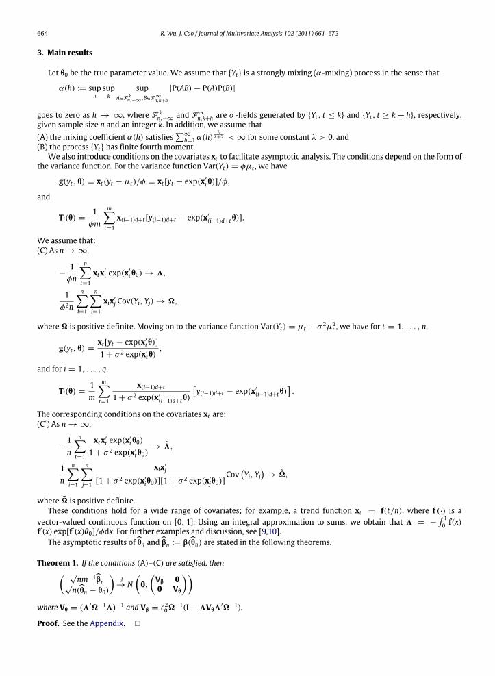
3. Main results

Let θ0 be the true parameter value. We assume that {Yt} is a strongly mixing (α-mixing) process in the sense that

α(h) := supn

supk

supA∈F k

n,−∞,B∈F ∞

n,k+h

|P(AB) − P(A)P(B)|

goes to zero as h → ∞, where F kn,−∞

and F ∞

n,k+h are σ -fields generated by {Yt , t ≤ k} and {Yt , t ≥ k + h}, respectively,given sample size n and an integer k. In addition, we assume that(A) the mixing coefficient α(h) satisfies

∑∞

h=1 α(h)λ

λ+2 < ∞ for some constant λ > 0, and(B) the process {Yt} has finite fourth moment.

We also introduce conditions on the covariates xt to facilitate asymptotic analysis. The conditions depend on the form ofthe variance function. For the variance function Var(Yt) = φµt , we have

g(yt , θ) = xt(yt − µt)/φ = xt [yt − exp(x′

tθ)]/φ,

and

Ti(θ) =1

φm

m−t=1

x(i−1)d+t [y(i−1)d+t − exp(x′

(i−1)d+tθ)].

We assume that:(C) As n → ∞,

−1φn

n−t=1

xtx′

t exp(x′

tθ0) → 3,

1φ2n

n−i=1

n−j=1

xix′

j Cov(Yi, Yj) → �,

where � is positive definite. Moving on to the variance function Var(Yt) = µt + σ 2µ2t , we have for t = 1, . . . , n,

g(yt , θ) =xt [yt − exp(x′

tθ)]

1 + σ 2 exp(x′tθ)

,

and for i = 1, . . . , q,

Ti(θ) =1m

m−t=1

x(i−1)d+t

1 + σ 2 exp(x′

(i−1)d+tθ)

y(i−1)d+t − exp(x′

(i−1)d+tθ).

The corresponding conditions on the covariates xt are:(C′) As n → ∞,

−1n

n−t=1

xtx′t exp(x

′tθ0)

1 + σ 2 exp(x′tθ0)

→ 3,

1n

n−i=1

n−j=1

xix′

j

[1 + σ 2 exp(x′

iθ0)][1 + σ 2 exp(x′

jθ0)]Cov

Yi, Yj

→ �,

where � is positive definite.These conditions hold for a wide range of covariates; for example, a trend function xt = f(t/n), where f (·) is a

vector-valued continuous function on [0, 1]. Using an integral approximation to sums, we obtain that 3 = − 10 f(x)

f′(x) exp[f′(x)θ0]/φdx. For further examples and discussion, see [9,10].The asymptotic results ofθn andβn := β(θn) are stated in the following theorems.

Theorem 1. If the conditions (A)–(C) are satisfied, then √nm−1βn√

n(θn − θ0)

d

→N0,Vβ 00 Vθ

where Vθ = (3′�−13)−1 and Vβ = c20�

−1(I − 3Vθ3′�−1).

Proof. See the Appendix. �


Remark 1. One virtue of specifying the variance function as V (z) = φz is that estimation of the scale parameter φ is notrequired for estimating the covariate coefficient vector θ and even for computing its asymptotic variance matrix. However,a φ estimate is required in order to estimate the asymptotic variance ofβn. Since Var(Yt) = φµt under this specification,we may estimate φ byφ =

∑nt=1(Yt −µt)

2/∑n

t=1µt .

Remark 2. It may be of interest to also perform statistical inferences for the scale parameter φ. In this regard, we need anadditional estimating function for φ. In the independent data case, for example, the constraint

∑nt=1{(yt −µt)

2/[φV (µt)]−1/φ} = 0 was used in [16, Section 4.2]. Alternatively, we may construct estimating functions based on Nelder andPregibon’s [22] extended quasi-likelihood. See also [13,4].

Theorem 2. If the conditions (A), (B), and (C′) are satisfied, then √nm−1βn√

n(θn − θ0)

d

→N0,Vβ 00 Vθ

,

where Vθ = (3′

�−1

3)−1 and Vβ = c20 �−1

(I − 3Vθ3′

�−1

).

The proof is similar to that of Theorem 1 and hence is omitted.As in the independent data case, for testing H0 : θ = θ0, we can use the blockwise empirical likelihood ratio statistic

WBE(θ0) defined by

WBE(θ0) = 2LBE(θ0) − 2LBE(θn). (2)

Theorem 3. Under the assumptions of Theorem 1, WBE(θ0) → χ2ℓ in distribution when H0 is true.

Proof. See the Appendix. �

Theorem 4. Under the assumptions of Theorem 2, WBE(θ0) → χ2ℓ in distribution when H0 is true.

The proof is similar to that of Theorem 3 and hence is omitted.

4. Simulation studies

Simulation studies were conducted to evaluate the finite sample performance of the proposed maximum blockwiseempirical likelihood estimator. We generated data from two models separately, which specify {Yt} as a sequence ofindependent random variables conditional on a latent process, with Poisson and geometric densities for the conditionaldistribution. More precisely, the two models are:

Model 1. Yt | αt ∼ Po(λt) and log(λt) = x′tθ + αt .

Model 2. Yt | αt ∼ Geo(pt) and log[(1 − pt)/pt ] = x′tθ + αt .

The latent process {αt} was specified by an AR(1) process: αt − µα = ρ(αt−1 − µα) + ζt , where {ζt} ∼ i.i.d. N(0, ς2).In order to satisfy the condition logµt(θ) = x′

tθ, we set µα = −σ 2α/2, where σ 2

α = ς2/(1 − ρ2) is the variance of αt .Otherwise, the intercept of the linear predictor is not identifiable. The value of the noise’s standard deviation ς was set to0.1, and three values of ρ, 0.1, 0.5, and 0.8, were considered. The covariate vector xt was defined to include a standardizedtrend and two harmonic function components, namely xt = (1, t/n, cos(2π t/6), sin(2π t/12))′, while the true coefficientvector was taken to be θ0 = (1, 1, 1, 0.5)′. For each model, we considered both forms of variance function: V (z) = φz andV (z) = z + σ 2z2. In addition, we took several combinations ofm and d values to study their effect on the estimation.

For each case, we simulated 100 replications and computed the empirical mean, bias, standard deviation (SD), and rootmean squared error (RMSE) of the estimates. The estimation technique performedwell in all cases overall, and the estimatesfollowed the asymptotic normal law. For succinctness, we only report here partial results, which are primarily based onsamples of size 500, to illustrate the effect of a single factor while holding the others identical. Tables 1–4 summarize thesimulation results for Model 1 with variance function V (z) = φz. Other results, which displayed a similar pattern, areincluded in the supplementary file (see the online version at doi:10.1016/j.jmva.2010.11.008) and are also available fromthe authors upon request.

Table 1 shows the effect of various selections of the block width m. As we can see, although all selected m values yield asatisfactory result, the intermediate values 8 and5performbetter. This is not always the case, however. The optimal selectionofm, which depends on the nature of a study, is as difficult a problem as bandwidth selection in nonparametric smoothing.As a practical guideline, the blockwidth can be selected using K -fold cross-validation. To be specific, the data are partitionedinto K folds. In each of the K experiments, we use K − 1 folds for training and the remaining one for testing. Let θ(−j) be theparameter estimates from theK−1 folds of data after removing the jth fold. And let Tℓ(θ(−j)) = 1/m

∑mt=1 g(y(ℓ−1)d+t , θ(−j)),

http://dx.doi.org/doi:10.1016/j.jmva.2010.11.008


Table 1The effect ofm; Model 1, V (z) = φz, n = 500, ρ = 0.5, and d = 2.

m = n5/12≈ 13

True Mean Bias × 102 SD RMSE

θ1 1.000 1.000 −0.009 0.050 0.050θ2 1.000 0.999 −0.143 0.076 0.076θ3 1.000 1.003 0.336 0.039 0.039θ4 0.500 0.499 −0.095 0.037 0.037

m = n3/8≈ 10


θ1 1.000 1.005 0.489 0.054 0.054θ2 1.000 0.996 −0.435 0.078 0.078θ3 1.000 0.996 −0.387 0.036 0.036θ4 0.500 0.500 −0.027 0.042 0.042

m = n1/3≈ 8


θ1 1.000 0.999 −0.122 0.048 0.048θ2 1.000 1.002 0.157 0.072 0.072θ3 1.000 1.002 0.224 0.030 0.030θ4 0.500 0.500 0.041 0.037 0.037

m = n1/4≈ 5


θ1 1.000 1.004 0.350 0.044 0.045θ2 1.000 0.997 −0.346 0.070 0.070θ3 1.000 0.995 −0.498 0.035 0.036θ4 0.500 0.500 −0.017 0.037 0.037

m = n1/6≈ 3


θ1 1.000 0.991 −0.865 0.050 0.050θ2 1.000 1.010 0.963 0.077 0.078θ3 1.000 1.007 0.740 0.034 0.034θ4 0.500 0.505 0.480 0.041 0.041

where ℓ ∈ Aj, the set of indices such that all y(ℓ−1)d+t , t = 1, . . . ,m, belong to the jth fold of data. Then, the block widthmis selected by minimizing

CV (m) =1K

K−j=1

−ℓ∈Aj

log[1 + β′

(−j)Tℓ(θ(−j))].

In our simulation studies K = 10 was used, which is common practice in the statistics literature. For the simulated data,on which Table 1 is based, the selection of m based on tenfold cross-validation agrees with that obtained using the RMSEcriterion. Table 2 shows the effect of different selections of d; since the block width is 8, the first panel of d = 8 implies thatthere is no overlap among blocks. It is well known that estimation is more efficient when the blocks overlap, with whichour results are in agreement: the smaller d, the better the estimation. Table 3 shows the effect of sample size. It is quiteclear that the estimates perform better as the sample size becomes larger. Table 4 shows the effect of the selection of ρ.It is not surprising that there is not much difference in estimation between the cases of ρ = 0.1 and ρ = 0.5. In bothcases, the dependence among the observed data is not so strong that the block width of 5 is sufficient to accommodatethe dependence. However, for the case of ρ = 0.8 there exists some bias in the coefficient estimates of the intercept andlinear trend. This is because, as the dependence among the data becomes stronger, larger block width becomes necessaryin order to account for the autocorrelation and ensure valid estimation. The asymptotic standard deviation ofθ can beobtained using Theorem 1. To be specific, firstly we evaluate the first two moments of the observed process Yt as follows:µt = exp(x′

tθ0),Var(Yt) = µt +µ2t Var(e

αt ), and Cov(Yi, Yj) = µiµj Cov(eαi , eαj) for i = j. But the autocovariance functionsof {eαt } are explicitly given in terms of those of {αt}, namely Cov(eαi , eαj) = exp(Cov(αi, αj)) − 1 for all i and j, whereCov(αi, αj) = ρ |i−j|σ 2

α for the specified AR(1) latent process. Therefore, the first two moments of Yt are readily computed.Then, the asymptotic variance ofθ is derived using the formula

n−

t=1

xtx′

t exp(x′

tθ0)

′ n−i=1

n−j=1

xix′

jCov(Yi, Yj)

−1 n−t=1

xtx′

t exp(x′

tθ0)

−1

.


Table 2The effect of d; Model 1, V (z) = φz, n = 500, ρ = 0.5, andm = 8.

d = 8


θ1 1.000 1.004 0.432 0.051 0.051θ2 1.000 0.989 −1.074 0.081 0.081θ3 1.000 1.005 0.461 0.032 0.032θ4 0.500 0.504 0.371 0.040 0.041

d = 4


θ1 1.000 1.000 −0.006 0.051 0.051θ2 1.000 1.005 0.474 0.079 0.079θ3 1.000 0.999 −0.094 0.032 0.032θ4 0.500 0.497 −0.317 0.036 0.036

d = 2


θ1 1.000 0.999 −0.122 0.048 0.048θ2 1.000 1.002 0.157 0.072 0.072θ3 1.000 1.002 0.224 0.030 0.030θ4 0.500 0.500 0.041 0.037 0.037

Table 3The effect of sample size n; Model 1, V (z) = φz, ρ = 0.5,m = 5, and d = 2.

n = 200

True Mean Bias × 102 SD RMSE ASD

θ1 1.000 1.001 0.128 0.072 0.072 0.077θ2 1.000 0.986 −1.362 0.107 0.108 0.114θ3 1.000 1.003 0.332 0.051 0.051 0.051θ4 0.500 0.506 0.566 0.066 0.066 0.060

n = 500


θ1 1.000 1.004 0.350 0.044 0.045 0.047θ2 1.000 0.997 −0.346 0.070 0.070 0.067θ3 1.000 0.995 −0.498 0.035 0.036 0.031θ4 0.500 0.500 −0.017 0.037 0.037 0.037

n = 1000


θ1 1.000 1.000 −0.001 0.035 0.035 0.033θ2 1.000 1.002 0.158 0.055 0.055 0.048θ3 1.000 1.000 −0.000 0.023 0.023 0.022θ4 0.500 0.502 0.231 0.029 0.029 0.026

The asymptotic standard deviation ofθ is (0.047, 0.067, 0.031, 0.037)′ for the cases in Tables 1 and 2,which does not dependon the selection ofm or d. In Table 1 the empirical standard deviationswhenm = 8 or 5 agree best with the asymptotic ones,which again supports the use of the RMSE and tenfold cross-validation as good criteria for the selection of block width. Onthe other hand, in Table 2 the empirical and asymptotic standard deviations are in the best agreement when d = 2, whichfurther illustrates the higher efficiency of overlapped blocks in the estimation. The asymptotic standard deviations for thecases in Tables 3 and 4 are reported correspondingly in the tables.

5. Applications

We applied blockwise empirical likelihood estimation to two empirical data sets: polio data, which consist of monthlycounts of poliomyelitis cases in the USA from the year 1970–1983 as reported by the Centers for Disease Control, and thedaily counts of non-accidental deaths from the year 1987–1996 in Toronto, Canada.

5.1. American monthly counts of poliomyelitis cases

The polio data have been analyzed by Zeger [31], Chan and Ledolter [2], Kuk and Cheng [17], Davis et al. [8,9], and Davisand Wu [10], among other researchers. Of central interest in the data is whether or not the rate of polio infection has been


Table 4The effect of ρ; Model 1, V (z) = φz, n = 500,m = 5, and d = 2.

ρ = 0.1


θ1 1.000 1.004 0.384 0.046 0.046 0.045θ2 1.000 0.994 −0.641 0.072 0.072 0.065θ3 1.000 1.003 0.347 0.034 0.034 0.031θ4 0.500 0.501 0.122 0.037 0.037 0.037

ρ = 0.5


θ1 1.000 1.004 0.350 0.044 0.045 0.047θ2 1.000 0.997 −0.346 0.070 0.070 0.067θ3 1.000 0.995 −0.498 0.035 0.036 0.031θ4 0.500 0.500 −0.017 0.037 0.037 0.037

ρ = 0.8


θ1 1.000 1.015 1.540 0.058 0.060 0.064θ2 1.000 0.980 −2.040 0.098 0.100 0.103θ3 1.000 0.997 −0.310 0.032 0.033 0.032θ4 0.500 0.496 −0.351 0.040 0.040 0.039

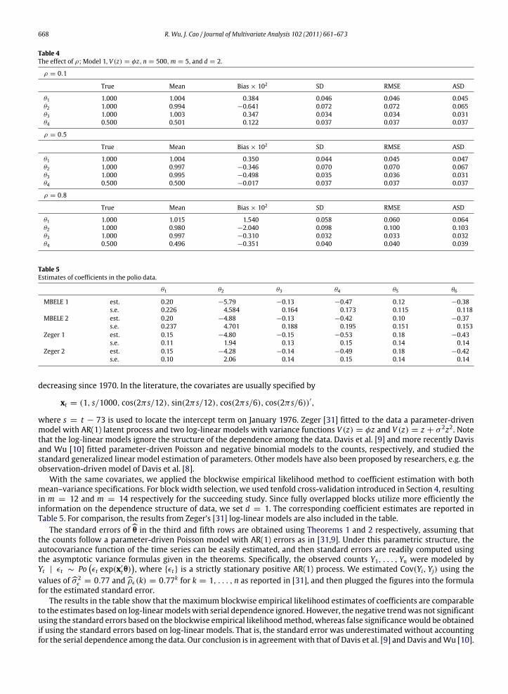
Table 5Estimates of coefficients in the polio data.

θ1 θ2 θ3 θ4 θ5 θ6

MBELE 1 est. 0.20 −5.79 −0.13 −0.47 0.12 −0.38s.e. 0.226 4.584 0.164 0.173 0.115 0.118

MBELE 2 est. 0.20 −4.88 −0.13 −0.42 0.10 −0.37s.e. 0.237 4.701 0.188 0.195 0.151 0.153

Zeger 1 est. 0.15 −4.80 −0.15 −0.53 0.18 −0.43s.e. 0.11 1.94 0.13 0.15 0.14 0.14

Zeger 2 est. 0.15 −4.28 −0.14 −0.49 0.18 −0.42s.e. 0.10 2.06 0.14 0.15 0.14 0.14

decreasing since 1970. In the literature, the covariates are usually specified by

xt = (1, s/1000, cos(2πs/12), sin(2πs/12), cos(2πs/6), cos(2πs/6))′,

where s = t − 73 is used to locate the intercept term on January 1976. Zeger [31] fitted to the data a parameter-drivenmodel with AR(1) latent process and two log-linear models with variance functions V (z) = φz and V (z) = z + σ 2z2. Notethat the log-linear models ignore the structure of the dependence among the data. Davis et al. [9] and more recently Davisand Wu [10] fitted parameter-driven Poisson and negative binomial models to the counts, respectively, and studied thestandard generalized linear model estimation of parameters. Other models have also been proposed by researchers, e.g. theobservation-driven model of Davis et al. [8].

With the same covariates, we applied the blockwise empirical likelihood method to coefficient estimation with bothmean–variance specifications. For block width selection, we used tenfold cross-validation introduced in Section 4, resultingin m = 12 and m = 14 respectively for the succeeding study. Since fully overlapped blocks utilize more efficiently theinformation on the dependence structure of data, we set d = 1. The corresponding coefficient estimates are reported inTable 5. For comparison, the results from Zeger’s [31] log-linear models are also included in the table.

The standard errors ofθ in the third and fifth rows are obtained using Theorems 1 and 2 respectively, assuming thatthe counts follow a parameter-driven Poisson model with AR(1) errors as in [31,9]. Under this parametric structure, theautocovariance function of the time series can be easily estimated, and then standard errors are readily computed usingthe asymptotic variance formulas given in the theorems. Specifically, the observed counts Y1, . . . , Yn were modeled byYt | ϵt ∼ Po

ϵt exp(x′

tθ), where {ϵt} is a strictly stationary positive AR(1) process. We estimated Cov(Yi, Yj) using the

values ofσ 2ϵ = 0.77 andρϵ(k) = 0.77k for k = 1, . . . , n as reported in [31], and then plugged the figures into the formula

for the estimated standard error.The results in the table show that the maximum blockwise empirical likelihood estimates of coefficients are comparable

to the estimates based on log-linearmodelswith serial dependence ignored. However, the negative trendwas not significantusing the standard errors based on the blockwise empirical likelihoodmethod, whereas false significancewould be obtainedif using the standard errors based on log-linear models. That is, the standard error was underestimated without accountingfor the serial dependence among the data. Our conclusion is in agreement with that of Davis et al. [9] and Davis andWu [10].


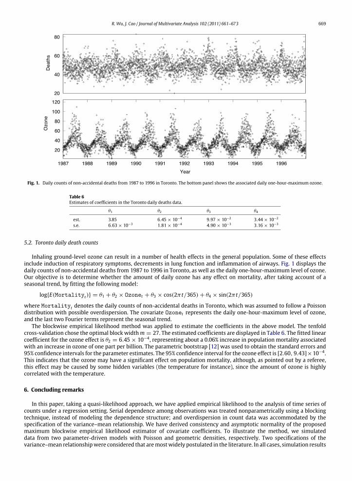
Fig. 1. Daily counts of non-accidental deaths from 1987 to 1996 in Toronto. The bottom panel shows the associated daily one-hour-maximum ozone.

Table 6Estimates of coefficients in the Toronto daily deaths data.

θ1 θ2 θ3 θ4

est. 3.85 6.45 × 10−4 9.97 × 10−2 3.44 × 10−2

s.e. 6.63 × 10−3 1.81 × 10−4 4.90 × 10−3 3.16 × 10−3

5.2. Toronto daily death counts

Inhaling ground-level ozone can result in a number of health effects in the general population. Some of these effectsinclude induction of respiratory symptoms, decrements in lung function and inflammation of airways. Fig. 1 displays thedaily counts of non-accidental deaths from 1987 to 1996 in Toronto, as well as the daily one-hour-maximum level of ozone.Our objective is to determine whether the amount of daily ozone has any effect on mortality, after taking account of aseasonal trend, by fitting the following model:

log{E(Mortalityt)} = θ1 + θ2 × Ozonet + θ3 × cos(2π t/365) + θ4 × sin(2π t/365)

where Mortalityt denotes the daily counts of non-accidental deaths in Toronto, which was assumed to follow a Poissondistribution with possible overdispersion. The covariate Ozonet represents the daily one-hour-maximum level of ozone,and the last two Fourier terms represent the seasonal trend.

The blockwise empirical likelihood method was applied to estimate the coefficients in the above model. The tenfoldcross-validation chose the optimal block widthm = 27. The estimated coefficients are displayed in Table 6. The fitted linearcoefficient for the ozone effect is θ2 = 6.45 × 10−4, representing about a 0.06% increase in population mortality associatedwith an increase in ozone of one part per billion. The parametric bootstrap [12] was used to obtain the standard errors and95% confidence intervals for the parameter estimates. The 95% confidence interval for the ozone effect is [2.60, 9.43]×10−4.This indicates that the ozone may have a significant effect on population mortality, although, as pointed out by a referee,this effect may be caused by some hidden variables (the temperature for instance), since the amount of ozone is highlycorrelated with the temperature.

6. Concluding remarks

In this paper, taking a quasi-likelihood approach, we have applied empirical likelihood to the analysis of time series ofcounts under a regression setting. Serial dependence among observations was treated nonparametrically using a blockingtechnique, instead of modeling the dependence structure; and overdispersion in count data was accommodated by thespecification of the variance–mean relationship. We have derived consistency and asymptotic normality of the proposedmaximum blockwise empirical likelihood estimator of covariate coefficients. To illustrate the method, we simulateddata from two parameter-driven models with Poisson and geometric densities, respectively. Two specifications of thevariance–mean relationshipwere considered that aremostwidely postulated in the literature. In all cases, simulation results


showed very good finite sample performance of the estimator. We also applied the blockwise empirical likelihood methodto two empirical data sets.

In the literature, applications of empirical likelihood to time series are usually confined to the cases of stationaryand continuous-valued time series. The present paper shows that empirical likelihood is also promising for analyzingnonstationary and/or discrete-valued time series data.

Acknowledgments

We thank the two referees for their helpful comments, which led to a significant improvement of the paper. RongningWu’s work was supported in part by The City University of New York PSC-CUNY Research Award 62561-00 40. Jiguo Cao’swork was supported in part by a discovery grant from the Natural Science and Engineering Research Council of Canada(NSERC).

Appendix

We first provide two lemmas used to establish Theorem 1.

Lemma 1. β(θ0) converges to zero in probability.

Proof. The function β(θ) solves the equations

1q

q−i=1

Ti(θ)

1 + β′Ti(θ)= 0. (3)

Like Owen [25], we write β(θ0) = uξ, where u ≥ 0 and ‖ξ‖ = 1 with ‖ · ‖ denoting the Euclidean norm. Then, we have

0 =1qξ′

q−i=1

Ti(θ0)

1 + uξ′Ti(θ0)

=1qξ′

q−i=1

Ti(θ0) −uqξ′

q−i=1

Ti(θ0)T′

i(θ0)

1 + uξ′Ti(θ0)ξ

≤ ξ′

1q

q−i=1

Ti(θ0)

−

uqξ′

q−i=1

Ti(θ0)T′

i(θ0)

1 + u max1≤i≤q

‖Ti(θ0)‖ξ.

Therefore,

u

ξ′

mq

q−i=1

Ti(θ0)T′

i(θ0)

ξ − mξ′

1q

q−i=1

Ti(θ0)

max1≤i≤q

‖Ti(θ0)‖

≤ mξ′

1q

q−i=1

Ti(θ0)

. (4)

The term on the right-hand side of (4) has an order of OP(mn−1/2). To see this, note that a mixing process is near-epochdependent in Lp norm on itself for all p ≥ 1. Applying a central limit theorem for near-epoch dependent processes [7], wehave

√mq

1q

q−i=1

Ti(θ0)

d

→N(0, �/c0).

Sincemq/n → 1/c0,

√n

1q

q−i=1

Ti(θ0)

d

→N(0, �).

That is,∑q

i=1 Ti(θ0)/q = OP(n−1/2). In addition, sincem = o(n1/2−1/τ ), it is easily shown using Lemma 3.2 of [18] that

max1≤i≤q

‖Ti(θ0)‖ = o(n1/2m−1)

almost surely. Therefore, the second term in the braces on the left-hand side of (4) has an order of oP(1). Also, it can beshown by Theorem 3 of [11] that

mq

q−i=1

Ti(θ0)T′

i(θ0)P

→ �/c0,


from which it follows that the first term in the braces on the left-hand side has an order of OP(1). Putting all the piecestogether, we obtain

u ≤OP(mn−1/2)

OP(1) − oP(1)= OP(mn−1/2).

That is, β(θ0) → 0 in probability. �

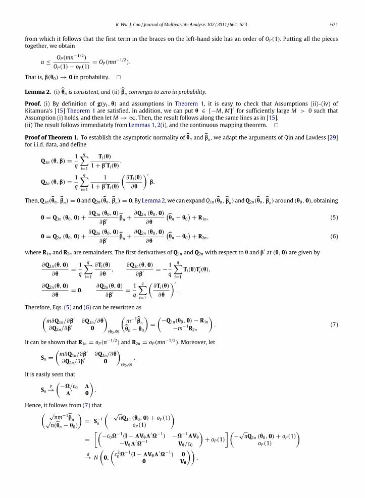
Lemma 2. (i)θn is consistent, and (ii)βn converges to zero in probability.

Proof. (i) By definition of g(yt , θ) and assumptions in Theorem 1, it is easy to check that Assumptions (ii)–(iv) ofKitamura’s [15] Theorem 1 are satisfied. In addition, we can put θ ∈ [−M,M]

ℓ for sufficiently large M > 0 such thatAssumption (i) holds, and then letM → ∞. Then, the result follows along the same lines as in [15].(ii) The result follows immediately from Lemmas 1, 2(i), and the continuous mapping theorem. �

Proof of Theorem 1. To establish the asymptotic normality ofθn andβn, we adapt the arguments of Qin and Lawless [29]for i.i.d. data, and define

Q1n (θ, β) =1q

q−i=1

Ti(θ)

1 + β′Ti(θ),

Q2n (θ, β) =1q

q−i=1

11 + β′Ti(θ)

∂Ti(θ)

∂θ

′

β.

Then,Q1n(θn,βn) = 0 andQ2n(θn,βn) = 0. By Lemma2,we can expandQ1n(θn,βn) andQ2n(θn,βn) around (θ0, 0), obtaining

0 = Q1n (θ0, 0) +∂Q1n (θ0, 0)

∂β′βn +

∂Q1n (θ0, 0)∂θ

θn − θ0+ R1n, (5)

0 = Q2n (θ0, 0) +∂Q2n (θ0, 0)

∂β′βn +

∂Q2n (θ0, 0)∂θ

θn − θ0+ R2n, (6)

where R1n and R2n are remainders. The first derivatives of Q1n and Q2n with respect to θ and β′ at (θ, 0) are given by

∂Q1n(θ, 0)∂θ

=1q

q−i=1

∂Ti(θ)

∂θ,

∂Q1n(θ, 0)∂β′

= −1q

q−i=1

Ti(θ)T′

i(θ),

∂Q2n(θ, 0)∂θ

= 0,∂Q2n(θ, 0)

∂β′=

1q

q−i=1

∂Ti(θ)

∂θ

′

.

Therefore, Eqs. (5) and (6) can be rewritten asm∂Q1n/∂β′ ∂Q1n/∂θ∂Q2n/∂β′ 0

(θ0,0)

m−1βnθn − θ0

=

−Q1n(θ0, 0) − R1n

−m−1R2n

. (7)

It can be shown that R1n = oP(n−1/2) and R2n = oP(mn−1/2). Moreover, let

Sn =

m∂Q1n/∂β′ ∂Q1n/∂θ∂Q2n/∂β′ 0

(θ0,0)

.

It is easily seen that

SnP

→

−�/c0 3

3′ 0

.

Hence, it follows from (7) that √nm−1βn√

n(θn − θ0)

= S−1

n

−

√nQ1n (θ0, 0) + oP(1)

oP(1)

=

[−c0�−1(I − 3Vθ3

′�−1) −�−13Vθ

−Vθ3′�−1 Vθ/c0

+ oP(1)

]−

√nQ1n (θ0, 0) + oP(1)

oP(1)

d

→ N0,c20�

−1(I − 3Vθ3′�−1) 0

0 Vθ

,


where the weak convergence results from√nQ1n (θ0, 0)

d→N(0, �). That is, √

nm−1βn√n(θn − θ0)

d

→N0,Vβ 00 Vθ

.

This completes the proof. �

Proof of Theorem 3. On the one hand,

LBE(θn,βn) =

q−i=1

log1 +β′

nTi(θn)

= β′

n

q−i=1

Ti(θ0) +β′

n

q−i=1

Vi(θ0)(θn − θ0) −12β′

n

q−i=1

Ti(θ0)T′

i(θ0)βn + oP(1)

= qm(m−1β′

n)Q1n(θ0, 0) + qm(m−1β′

n)3(θn − θ0) −qm2

(m−1β′

n) (�/c0) (m−1βn) + oP(1)

= c0qmQ′

1n (θ0, 0) �−1 I − 3Vθ3′�−1Q1n (θ0, 0)

+ c0qmQ′

1n (θ0, 0) �−1 I − 3Vθ3′�−13

Vθ3

′�−1Q1n (θ0, 0)

−c0qm2

Q′

1n (θ0, 0) �−1 I − 3Vθ3′�−1��−1 I − 3Vθ3

′�−1Q1n (θ0, 0) + oP(1)

=c0qm2

Q′

1n (θ0, 0)�−1

− �−13Vθ3′�−1Q1n (θ0, 0) + oP(1).

On the other hand, using the fact that∑q

i=1 Ti(θ0)/[1 + β′

0Ti(θ0)] = 0, a Taylor expansion about β0 at zero yieldsm−1β0 = (�/c0)−1Q1n(θ0, 0) + oP(n−1/2). Then,

LBEθ0, β0

=

q−i=1

log1 + β′

0Ti(θ0)

= β′

0

q−i=1

Ti(θ0) −12β′

0

q−i=1

Ti(θ0)T′

i(θ0)β0 + oP(1)

= qmm−1β′

0

Q1n (θ0, 0) −

qm2

m−1β′

0

(�/c0)

m−1β0

+ oP(1)

= c0qmQ′

1n (θ0, 0) �−1Q1n (θ0, 0) −c0qm2

Q′

1n (θ0, 0) �−1��−1Q1n (θ0, 0) + oP(1)

=c0qm2

Q′

1n (θ0, 0) �−1Q1n (θ0, 0) + oP(1).

So,

WBE(θ0) = c0qmQ′

1n (θ0, 0) �−13Vθ3′�−1Q1n (θ0, 0) + oP(1)

=(�/c0)−1/2 √

mqQ1n (θ0, 0)′

�−1/23Vθ3′�−1/2 (�/c0)−1/2 √

mqQ1n (θ0, 0)+ oP(1).

Note that (�/c0)−1/2 √mqQ1n (θ0, 0)

d→N(0, Iℓ); moreover, �−1/23Vθ3

′�−1/2 is symmetric and idempotent with trace

equal to ℓ. Therefore,WBE(θ0)d

→ χ2ℓ , which is the desired result. �

References

[1] F. Bravo, Blockwise generalized empirical likelihood inference for non-linear dynamic moment conditions models, Econometrics Journal 12 (2009)208–231.

[2] K.S. Chan, J. Ledolter, Monte Carlo EM estimation for time series models involving counts, Journal of the American Statistical Association 90 (1995)242–252.

[3] N.H. Chan, S. Ling, Empirical likelihood for GARCH models, Econometric Theory 22 (2006) 403–428.[4] S.X. Chen, H. Cui, An extended empirical likelihood for generalized linear models, Statistica Sinica 13 (2003) 69–81.[5] C.S. Chuang, N.H. Chan, Empirical likelihood for autoregressive models, with applications to unstable time series, Statistica Sinica 12 (2002) 387–407.[6] D.R. Cox, Statistical analysis of time series: some recent developments, Scandinavian Journal of Statistics 8 (1981) 93–115.[7] J. Davidson, A central limit theorem for globally nonstationary near-epoch dependent functions of mixing processes, Econometric Theory 8 (1992)

313–329.[8] R.A. Davis, W.T.M. Dunsmuir, Y. Wang, Modeling time series of count data, in: S. Ghosh (Ed.), Asymptotics, Nonparametrics and Time Series, Marcel

Dekker, New York, 1999, pp. 63–114.[9] R.A. Davis, W.T.M. Dunsmuir, Y. Wang, On autocorrelation in a Poisson regression model, Biometrika 87 (2000) 491–505.

[10] R.A. Davis, R. Wu, A negative binomial model for time series of counts, Biometrika 96 (2009) 735–749.[11] R.M. de Jong, Laws of large numbers for dependent heterogeneous processes, Econometric Theory 11 (1995) 347–358.


[12] B. Efron, R.J. Tibshirani, An Introduction to the Bootstrap, Chapman and Hall, New York, 1993.[13] V.P. Godambe, M.E. Thompson, An extension of quasi-likelihood estimation, Journal of Statistical Planning and Inference 22 (1989) 137–152.[14] C. Gourieroux, A. Monfort, A. Trognon, Pseudo maximum likelihood methods: applications to Poisson models, Econometrica 52 (1984) 701–720.[15] Y. Kitamura, Empirical likelihood methods with weakly dependent processes, Annals of Statistics 25 (1997) 2084–2102.[16] E.D. Kolaczyk, Empirical likelihood for generalized linear models, Statistica Sinica 4 (1994) 199–218.[17] A.Y.C. Kuk, Y.W. Cheng, The Monte Carlo Newton–Raphson algorithm, Journal of Statistical Computation and Simulation 59 (1997) 233–250.[18] H.R. Künsch, The jackknife and the bootstrap for general stationary observations, Annals of Statistics 17 (1989) 1217–1241.[19] P. McCullagh, J.A. Nelder, Generalized Linear Models, 2nd ed., Chapman and Hall, London, 1989.[20] A.C. Monti, Empirical likelihood confidence regions in time series models, Biometrika 84 (1997) 395–405.[21] P.A. Mykland, Dual likelihood, Annals of Statistics 23 (1995) 396–421.[22] J.A. Nelder, D. Pregibon, An extended quasi-likelihood function, Biometrika 74 (1987) 221–232.[23] D.J. Nordman, P. Sibbertsen, S.N. Lahiri, Empirical likelihood confidence intervals for the mean of a long-range dependent process, Journal of Time

Series Analysis 28 (2007) 576–599.[24] A.B. Owen, Empirical likelihood ratio confidence intervals for a single functional, Biometrika 75 (1988) 237–249.[25] A.B. Owen, Empirical likelihood ratio confidence regions, Annals of Statistics 18 (1990) 90–120.[26] A.B. Owen, Empirical likelihood for linear models, Annals of Statistics 19 (1991) 1725–1747.[27] A.B. Owen, Empirical Likelihood, Chapman and Hall/CRC, 2001.[28] D.N. Politis, J.P. Romano, A general resampling scheme for triangular arrays of α-mixing random variables with application to the problem of spectral

density estimation, Annals of Statistics 20 (1992) 1985–2007.[29] J. Qin, J. Lawless, Empirical likelihood and general estimating equations, Annals of Statistics 22 (1994) 300–325.[30] R.W.M. Wedderburn, Quasi-likelihood functions, generalized linear models, and the Gauss–Newton method, Biometrika 61 (1974) 439–447.[31] S.L. Zeger, A regression model for time series of counts, Biometrika 75 (1988) 621–629.[32] S.L. Zeger, B. Qaqish, Markov regression models for time series: a quasi-likelihood approach, Biometrics 44 (1988) 1019–1031.

Blockwise empirical likelihood for time series of counts

Documents

Transcript of Blockwise empirical likelihood for time series of counts