A frequency domain empirical likelihood

for short- and long-range dependence∗

Short Title: Spectral empirical likelihood

Daniel J. Nordman & Soumendra N. Lahiri

Dept. of Statistics

Iowa State University

Ames, IA 50011 USA

Abstract

This paper introduces a version of empirical likelihood based on the periodogram and spec-

tral estimating equations. This formulation handles dependent data through a data trans-

formation (i.e., Fourier transform) and is developed in terms of the spectral distribution

rather than a time domain probability distribution. The asymptotic properties of frequency

domain empirical likelihood are studied for linear time processes exhibiting both short- and

long-range dependence. The method results in likelihood ratios which can be used to build

nonparametric, asymptotically correct confidence regions for a class of normalized (or ratio)

spectral parameters, including autocorrelations. Maximum empirical likelihood estimators

are possible as well as tests of spectral moment conditions. The methodology can be applied

to several inference problems, such as Whittle estimation and goodness-of-fit testing.

1 Introduction

The main contribution of this paper is a new formulation of empirical likelihood (EL) for

inference with two fundamentally different types of dependent data: time series exhibiting

either short-range dependence (SRD) or long-range dependence (LRD). Let {Xt}, t ∈ Z, be a

∗AMS 2000 subject classifications: Primary-62F40, 62G09; secondary- 62G20. Key Words: Empirical

likelihood, estimating equations, long-range dependence, periodogram, spectral distribution, Whittle esti-

mation

1

stationary sequence of random variables with mean µ and spectral density f on Π = [−π, π]

where

f(λ) ∼ C(α)|λ|−α, λ → 0 (1)

for α ∈ [0, 1) and a constant C(α) > 0 involving α (with ∼ indicating the terms have a ratio

of one in the limit). When α = 0, we classify the process {Xt} as short-range dependent

(SRD). For α > 0, the process will be called long-range dependent (LRD). This classification

resembles the one from [26] and encompasses the formulation of LRD described in [4, 40].

Originally proposed by [33, 34] for independent samples, EL allows for nonparametric

likelihood-based inference with a broad range of applications [36]. An important bene-

fit of EL inference is that confidence regions for parameters may be calibrated through

log-likelihood ratios, without requiring any direct estimates of variance or skewness [20].

However, a difficulty with extending EL methods to dependent data is then to ensure that

“correct” variance estimation occurs automatically within EL ratios under the data depen-

dence structure. This is an important reason why the EL version for iid data from [34] does

not apply to dependent data (see [24], p. 2085).

Recent extensions of EL to time series in [24, 31] have relied exclusively on a SRD

structure with rapidly decreasing process correlations. In particular, [24] provided a break-

through formulation of EL for weakly dependent data based on data blocks rather than

individual observations. Under SRD, the resulting blockwise EL ratios correctly perform

variance estimation of sample means within their mechanics. Data blocking has also proven

to be crucial in extending other nonparametric likelihoods to weakly dependent processes,

such as the block bootstrap and resampling methods described in [27], Chapter 2.

In comparison to weak dependence, the rate of decay of the covariance function r(k) =

Cov(Xj , Xj+k) is characteristically much slower under strong dependence α > 0, namely:

r(k) ∼ C(α)k−(1−α), k →∞, (2)

with a constant C(α) > 0, which is an alternative representation of LRD (with equivalence

to (1) if the covariances converge quasimonotically to zero; see p. 1632 of [40]). This

autocovariance behavior implies that statistical procedures developed for SRD may not be

applicable under LRD, often due to complications with variance estimation. For example,

the moving block bootstrap is known to be invalid under strong dependence for inference

on the process mean EXt = µ [25], partly because (2) implies that the variance Var(Xn) =

O(n−1+α) of a size n sample mean exhibits a slower, unknown rate of decay compared to

the O(n−1) rate associated with SRD data. For this reason, the blockwise EL formulation

of [24] will also break down under strong dependence for inference on the mean.

In this paper, we formulate an EL based on the periodogram combined with certain

2

estimating equations. Using this data transformation to weaken the underlying dependence

structure, the resulting frequency domain empirical likelihood (FDEL) provides a common

tool for nonparametric inference on both SRD and LRD time series. Because this EL version

involves the spectral distribution of a time process rather than a time domain probability

distribution, inference is restricted to a class of normalized spectral parameters described in

Section 2. The frequency domain bootstrap (FDB) of [12], developed for SRD, targets the

same class of parameters. Hence, for parameters not defined in terms of the spectral density

(e.g., the process mean µ), the FDEL is inapplicable while the time domain blockwise EL in

[24] may still be valid if the process exhibits SRD (i.e., valid for a larger class of parameters

under weak dependence).

Our main result is the asymptotic distribution of FDEL ratio statistics, which are shown

to have limiting chi-square distributions under both SRD and LRD for setting confidence

regions. That is, FDEL shares the strength of EL methods to incorporate “correct” variance

estimation for spectral parameter inference automatically in its mechanics. For normalized

spectral parameters where both the FDB and blockwise EL may be applicable under SRD

(e.g., autocorrelations), the FDEL requires no kernel density estimates of f (as with the

FDB) and no block selection (as with the blockwise EL). Our FDEL results also refine some

EL theory given in [31], who proposed periodogram-based EL confidence regions for Whittle-

type estimation with SRD linear processes. We additionally consider FDEL tests, based on

maximum EL estimation, which are helpful for assessing both parameter conjectures and

the validity of (spectral) moment conditions, as in the independent data EL formulation

[34, 38].

The methodology presented here is applicable to linear processes with spectral densi-

ties satisfying (1), which includes two common models for LRD processes: the fractional

Gaussian processes of [29] with spectral density

fH,σ2(λ) =4σ2Γ(2H − 1)

(2π)2H+2cos(πH − π/2) sin2(λ/2)

∞∑

k=−∞|λ/(2π) + k|−1−2H , λ ∈ Π, (3)

1/2 < H < 1, and the fractional autoregressive integrated moving average (FARIMA)

processes of [1, 19, 22] with spectral density

fd,ρ,%,σ2(λ) =σ2

2π|1− eıλ|−2d

∣∣∣∣∣

∑pj=0 ρj

(eıλ

)j

∑qj=0 %j (eıλ)j

∣∣∣∣∣

2

, λ ∈ Π, (4)

based on parameters 0 < d < 1/2, ρ = (ρ1, . . . , ρp), % = (%1, . . . , %q) with ρ0 = %0 = 1 and

ı =√−1. These models fulfill (1) with α = 2H − 1 and α = 2d, respectively.

The rest of the paper is organized as follows. Section 2 describes the role of spectral

estimating equations for FDEL inference and several examples are given. In Section 3, we

3

explain the construction of EL in the frequency domain. Section 4 contains the Assump-

tions and the main results on the distribution of FDEL log-ratios for confidence region

estimation and simple hypothesis testing. In Section 5, we consider maximum EL estima-

tion in the frequency domain. We describe the application of FDEL to Whittle estimation

in Section 6, while Section 7 considers goodness-of-fit testing with FDEL. Section 8 offers

some conclusions. Proofs of the results are given in Sections 9 and 10.

2 Spectral estimating equations

Consider inference on a parameter θ ∈ Θ ⊂ IRp based on a time stretch X1, . . . , Xn. Fol-

lowing the EL framework of [38, 39] with iid data, we suppose that information about θ

exists through a system of general estimating equations. However, we will use the process

spectral distribution to define moment conditions as follows. Let

Gθ(λ) = (g1,θ(λ), . . . , gr,θ(λ))′ : Π×Θ → IRr (5)

denote a vector of even, estimating functions with r ≥ p. For the case r > p, the above

functions are said to be “overidentifying” for θ. We assume that Gθ satisfies the spectral

moment condition ∫ π

0Gθ0(λ)f(λ)dλ = M (6)

for some known M∈ IRr at the true value θ0 of the parameter. As distributional results in

Section 4 indicate, we will typically require M = 0, which places some restrictions on the

types of spectral parameters considered. However, FDEL framework is valid for estimating

normalized spectral means: θ =∫ π0 Gfdλ/

∫ π0 fdλ based on a vector function G. The FDB

targets the same parameters under SRD and [12] comments on the importance, and often

complete adequacy, of population information expressed in this ratio form. The FDEL

construction in Section 3 combines the periodogram with the estimating equations in (6).

2.1 Examples

We provide a few examples of useful estimating functions for inference, some of which sat-

isfy (5) with M = 0.

Example 1: Autocorrelations. Consider interest in the autocorrelation function ρ(·) at

arbitrary lags m1, . . . , mp; that is, θ = (ρ(m1), . . . , ρ(mp))′ where

ρ(m) = r(m)/r(0) =∫ π

0cos(mλ)f(λ)dλ

/ ∫ π

0f(λ)dλ, m ∈ Z.

4

One can select Gθ(λ) = (cos(m1λ), . . . , cos(mpλ))′−θ for autocorrelation inference, fulfilling

(6) with M = 0 ∈ IRp and r = p.

Example 2: Spectral distribution function. For ω ∈ [0, π], denote the spectral dis-

tribution function as F (ω) =∫ ω0 f(λ)dλ. Suppose θ = (F (τ1)/F (π), . . . , F (τp)/F (π))′

for some τ1, . . . τp ∈ (0, π). This normalized parameter θ often sufficiently characterizes

the spectral distribution F for testing purposes [10]. For inference on θ, we can pick

Gθ(λ) = (11{λ ≤ τ1}, . . . , 11{λ ≤ τp})′ − θ where 11{·} denotes the indicator function. Then

(6) holds with spectral mean M = 0 ∈ IRp.

Example 3: Goodness-of-fit tests. There has been increasing interest in frequency

domain-based tests to assess model adequacy [2, 37]. Consider a test involving a simple null

hypothesis H0 : f = f0 against an alternative H1 : f 6= f0 for some candidate density f0.

With EL techniques, one immediate test for H0 is based on the function G0(λ) = 1/f0(λ)

with spectral mean π under H0; here we treat r = 1 and the dimension p of θ as 0. We

show in Section 7 that a EL ratio test results which resembles a spectral goodness-of-fit test

statistic proposed by [30] and shown by [3] to be useful for LRD Gaussian series. The more

interesting and complicated problem of testing the hypothesis that f belongs to a given

model family can also be addressed with FDEL, as discussed in Section 7.

Example 4: Whittle estimation. We denote a parametric collection of spectral densities

as

F = {fθ(λ) : θ ∈ Θ} (7)

and assume the densities are positive on Π and identifiable (e.g., for θ 6= θ ∈ Θ, the Lebesgue

measure of {λ : fθ(λ) 6= fθ(λ)} is positive). For fitting the model fθ to the data, Whittle

estimation [42] seeks the θ-value at which the theoretical “distance” measure

W (θ) = (4π)−1

∫ π

0

{log fθ(λ) +

f(λ)fθ(λ)

}dλ (8)

achieves its minimum [14]. The model class may be misspecified (possibly f /∈ F) but

Whittle estimation aims for the density in F “closest” to f as measured by W (θ).

To consider a particular parameterization of (7), suppose

fθ(λ) = σ2kϑ(λ), θ = (σ2, ϑ′)′, Θ ⊂ (0,∞)× IRp−1, ϑ = (ϑ1, . . . , ϑp−1)′, (9)

with kernel density kϑ and that Kolmogorov’s formula holds with (2π)−1∫ π−π log fθ(λ)dλ =

log[σ2/(2π)] (e.g., taking σ2 as the innovation variance in a linear model). The model class in

(9) is commonly considered in the context of Whittle estimation for both SRD and LRD time

5

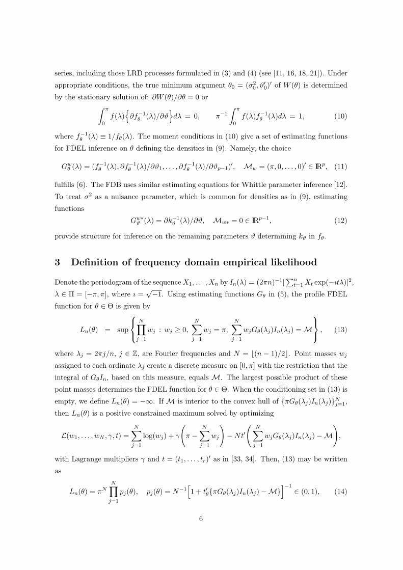
series, including those LRD processes formulated in (3) and (4) (see [11, 16, 18, 21]). Under

appropriate conditions, the true minimum argument θ0 = (σ20, ϑ

′0)′ of W (θ) is determined

by the stationary solution of: ∂W (θ)/∂θ = 0 or∫ π

0f(λ)

{∂f−1

θ (λ)/∂ϑ}

dλ = 0, π−1

∫ π

0f(λ)f−1

θ (λ)dλ = 1, (10)

where f−1θ (λ) ≡ 1/fθ(λ). The moment conditions in (10) give a set of estimating functions

for FDEL inference on θ defining the densities in (9). Namely, the choice

Gwθ (λ) = (f−1

θ (λ), ∂f−1θ (λ)/∂ϑ1, . . . , ∂f−1

θ (λ)/∂ϑp−1)′, Mw = (π, 0, . . . , 0)′ ∈ IRp, (11)

fulfills (6). The FDB uses similar estimating equations for Whittle parameter inference [12].

To treat σ2 as a nuisance parameter, which is common for densities as in (9), estimating

functions

Gw∗ϑ (λ) = ∂k−1

ϑ (λ)/∂ϑ, Mw∗ = 0 ∈ IRp−1, (12)

provide structure for inference on the remaining parameters ϑ determining kϑ in fθ.

3 Definition of frequency domain empirical likelihood

Denote the periodogram of the sequence X1, . . . , Xn by In(λ) = (2πn)−1|∑nt=1 Xt exp(−ıtλ)|2,

λ ∈ Π = [−π, π], where ı =√−1. Using estimating functions Gθ in (5), the profile FDEL

function for θ ∈ Θ is given by

Ln(θ) = sup

N∏

j=1

wj : wj ≥ 0,N∑

j=1

wj = π,N∑

j=1

wjGθ(λj)In(λj) = M , (13)

where λj = 2πj/n, j ∈ Z, are Fourier frequencies and N = b(n − 1)/2c. Point masses wj

assigned to each ordinate λj create a discrete measure on [0, π] with the restriction that the

integral of GθIn, based on this measure, equals M. The largest possible product of these

point masses determines the FDEL function for θ ∈ Θ. When the conditioning set in (13) is

empty, we define Ln(θ) = −∞. If M is interior to the convex hull of {πGθ(λj)In(λj)}Nj=1,

then Ln(θ) is a positive constrained maximum solved by optimizing

L(w1, . . . , wN , γ, t) =N∑

j=1

log(wj) + γ

(π −

N∑

j=1

wj

)−Nt′

(N∑

j=1

wjGθ(λj)In(λj)−M)

,

with Lagrange multipliers γ and t = (t1, . . . , tr)′ as in [33, 34]. Then, (13) may be written

as

Ln(θ) = πNN∏

j=1

pj(θ), pj(θ) = N−1[1 + t′θ{πGθ(λj)In(λj)−M}

]−1∈ (0, 1), (14)

6

where tθ is the stationary point of the function q(t) =∑N

j=1 log(1+t′{πGθ(λj)In(λj)−M}).(See [34, 38] for further computational details on EL.) Without the integral-type linear

constraint in (13),∏N

j=1 wj has a maximum when each wj = π/N so that we can form a

profile EL ratio:

Rn(θ) = Ln(θ)/(

πN−1)N =

N∏

j=1

[1 + t′θ{πGθ(λj)In(λj)−M}

]−1. (15)

3.1 A density-based formulation of empirical likelihood

To help frame the EL results here to those in [31], we give an alternative, model-based

formulation of FDEL. This version requires a density class F as in (7) and involves ap-

proximating the expected value E(In(λj)) with fθ(λj) using a density fθ ∈ F . Namely,

let

Ln,F(θ) = sup

N∏

j=1

wj : wj ≥ 0,N∑

j=1

wj = π,N∑

j=1

wjGθ(λj)[In(λj)− fθ(λj)] = 0

Rn,F(θ) = (N/π)NLn,F(θ). (16)

We consider the densities fθ and prospective functions Gθ as dependent on the same pa-

rameters which causes no loss of generality. An exact form for Ln,F(θ) can be deduced as

with Ln(θ), obtained by replacing In(λj),M with In(λj)− fθ, 0 in (14).

Section 6 discusses the model-based EL ratio in (16) for refining results in [31] on confi-

dence interval estimation of Whittle parameters. This version of FDEL may additionally be

suitable for conducting goodness-of-fit tests with respect to a family of spectral densities.

4 Main Result: Distribution of empirical likelihood ratio

Before describing the distributional properties of FDEL, we set some assumptions on the

time process under consideration and the potential vector of estimating functions Gθ in (5).

4.1 Assumptions

In the following, let θ0 denote the unique (true) parameter value which satisfies (6).

Assumptions

(A.1) {Xt} is a real-valued, linear process with a moving average representation of the

form:

Xt = µ +∞∑

j=−∞bjεt−j , t ∈ Z

7

where {εt} are iid random variables with E(εt) = 0, E(ε2t ) = σ2

ε > 0, E(ε8t ) < ∞ and 4-th

order cumulant denoted as κ4,ε ≡ E(ε4t ) − 3σ4

ε ; {bt} is a sequence of constants satisfying∑

t∈Z b2t < ∞ and b0 = 1; and f(λ) = σ2

ε |b(λ)|2/(2π), λ ∈ Π with b(λ) =∑

j∈Z bjeıjλ.

It is assumed that f(λ) is continuous on (0, π] and that f(λ) ≤ C|λ|−α, λ ∈ Π, for some

α ∈ [0, 1), C > 0.

(A.2) Each component gj,θ0 of Gθ0 is an even, integrable function such that |gj,θ0(λ)| ≤C|λ|β, λ ∈ Π, where 0 ≤ β < 1, α− β < 1/2, j = 1, . . . , r.

(A.3) For each gj,θ0(λ), j = 1, . . . , r, one of the following is fulfilled:

Condition 1. gj,θ0 is Lipschitz of order greater than 1/2 on [0, π].

Condition 2. gj,θ0 is continuous on Π and |∂gj,θ0(λ)/∂λ| ≤ C|λ|βj−1 for some 0 ≤ βj < 1,

2α− βj < 1.

Condition 3. gj,θ0 is of bounded variation on [0, π] with finite discontinuities and α < 1/2

with |r(k)| ≤ Ck−υ for some υ > 1/2 (e.g., υ = 1− α).

(A.4) The r × r matrix Wθ0 =∫Π f2(λ)Gθ0(λ)G′

θ0(λ)dλ is positive definite.

(A.5) On (0, π], f is differentiable and |∂f(λ)/∂λ| ≤ C|λ|−α−1; or each f(λ)gj,θ0(λ) is of

bounded variation or is piecewise Lipschitz of order greater than 1/2 on [0, π], j = 1, . . . , r.

As n →∞, P (0 ∈ ch◦{πGθ0(λj)[In(λj)− f(λj)]}Nj=1) → 1, where ch◦A denotes the interior

convex hull of a finite set A ⊂ IRr.

We briefly discuss the assumptions. The bound on f in Assumption A.1 allows for the

process {Xt} to exhibit both SRD and LRD and is a slight generalization of (1). The behav-

ior of Gθ0 in Assumption A.2 controls the growth rate of the scaled periodogram ordinates,

Gθ0(λj)In(λj), at low frequencies under LRD and ensures that Wθ0 is finite. Important

processes are permissible under A.1 and, for these, useful estimating functions often satisfy

A.2. Assumption A.3 outlines smoothness criteria for the estimating functions. The esti-

mating functions treated by the FDB in [12] meet A.3, including those for autocorrelations

and normalized spectral distribution in Section 2.1. The functions f−1θ and ∂f−1

θ /∂θ from

Examples 3 and 4 satisfy A.3 with many SRD and LRD models for use in Whittle-like

estimation and goodness-of-fit testing in the FDEL framework. For example, [21] considers

Whittle estimation for ARMA densities for which functions Gwθ in (11) meet Condition 1.

The functions f−1θ and ∂fθ/∂θ associated with the fractional Gaussian and FARIMA LRD

densities in (3) and (4) fulfill Condition 2 [11, 16, 18]. Process dependence that is not

8

extremely strong, so that f2 is integrable, allows greater flexibility in choosing more general

estimating functions in Condition 3.

For EL inference exclusively with the model-based functions Ln,F or Rn,F from Sec-

tion 3.1, we use an additional assumption A.5 which is generally not restrictive. The

probabilistic condition in A.5 implies only that the EL ratio Rn,F can be finitely computed

at θ0, resembling EL assumptions of [31] and [35].

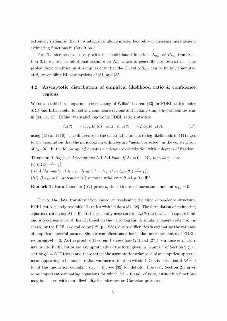
4.2 Asymptotic distribution of empirical likelihood ratio & confidence

regions

We now establish a nonparametric recasting of Wilks’ theorem [43] for FDEL ratios under

SRD and LRD, useful for setting confidence regions and making simple hypothesis tests as

in [33, 34, 35]. Define two scaled log-profile FDEL ratio statistics:

`n(θ) = −4 log Rn(θ) and `n,F(θ) = −2 log Rn,F(θ), (17)

using (15) and (16). The difference in the scalar adjustments to log-likelihoods in (17) owes

to the assumption that the periodogram ordinates are “mean-corrected” in the construction

of `n,F(θ). In the following, χ2ν denotes a chi-square distribution with ν degrees of freedom.

Theorem 1 Suppose Assumptions A.1-A.4 hold. If M = 0 ∈ IRr, then as n →∞(i) `n(θ0)

d−→ χ2r.

(ii) Additionally, if A.5 holds and f = fθ0, then `n,F(θ0)d−→ χ2

r.

(iii) If κ4,ε = 0, statement (ii) remains valid even if M 6= 0 ∈ IRr.

Remark 1: For a Gaussian {Xt} process, the 4-th order innovation cumulant κ4,ε = 0.

Due to the data transformation aimed at weakening the time dependence structure,

FDEL ratios closely resemble EL ratios with iid data [34, 38]. The formulation of estimating

equations satisfying M = 0 in (6) is generally necessary for `n(θ0) to have a chi-square limit

and is a consequence of this EL based on the periodogram. A similar moment restriction is

shared by the FDB, as detailed by [12] (p. 1938), due to difficulties in estimating the variance

of empirical spectral means. Similar complications arise in the inner mechanics of FDEL,

requiring M = 0. As the proof of Theorem 1 shows (see (24) and (27)), variance estimators

intrinsic to FDEL ratios are asymptotically of the form given in Lemma 7 of Section 9 (i.e.,

setting gh = GG′ there) and these target the asymptotic variance V of an empirical spectral

mean appearing in Lemma 6 so that variance estimation within FDEL is consistent ifM = 0

(or if the innovation cumulant κ4,ε = 0); see [32] for details. However, Section 2.1 gives

some important estimating equations for which M = 0 and, of note, estimating functions

may be chosen with more flexibility for inference on Gaussian processes.

9

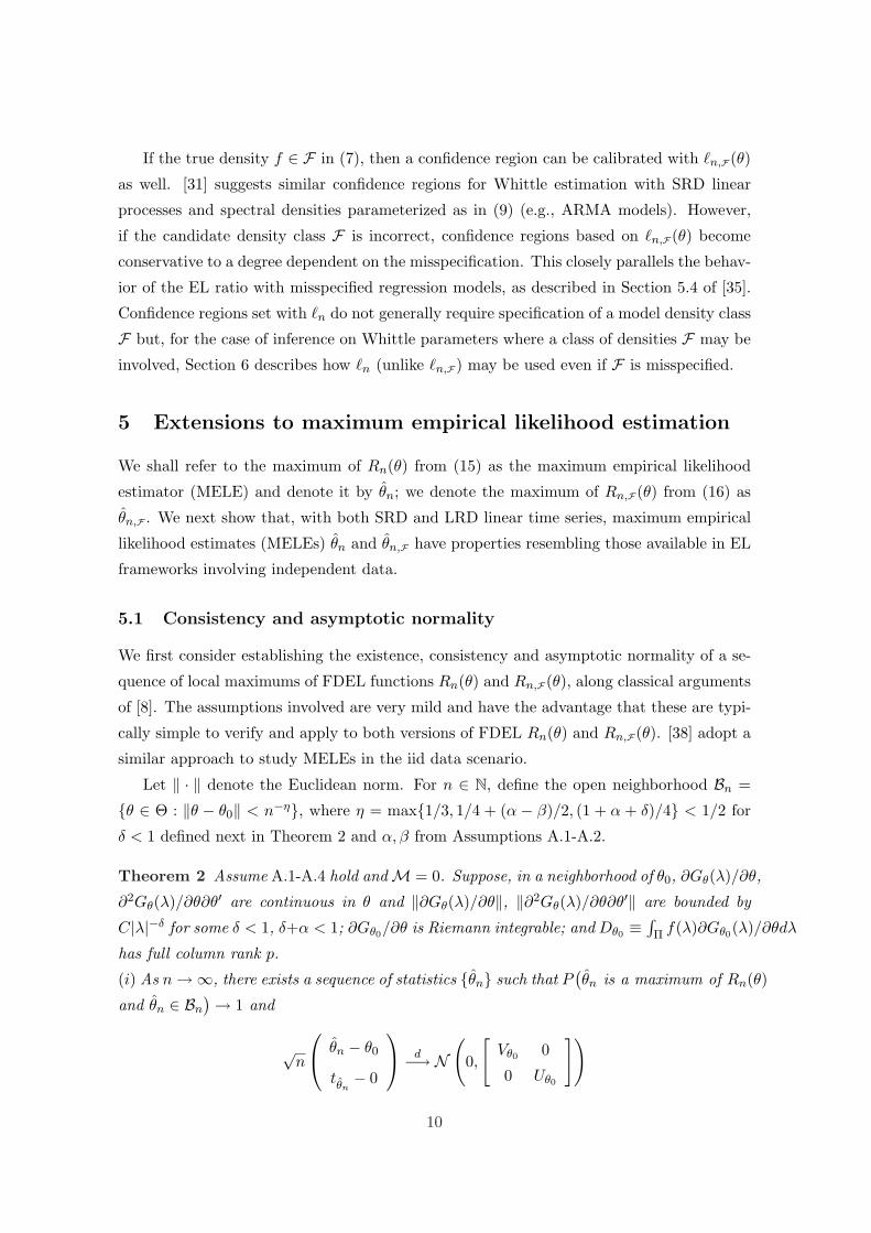
If the true density f ∈ F in (7), then a confidence region can be calibrated with `n,F(θ)

as well. [31] suggests similar confidence regions for Whittle estimation with SRD linear

processes and spectral densities parameterized as in (9) (e.g., ARMA models). However,

if the candidate density class F is incorrect, confidence regions based on `n,F(θ) become

conservative to a degree dependent on the misspecification. This closely parallels the behav-

ior of the EL ratio with misspecified regression models, as described in Section 5.4 of [35].

Confidence regions set with `n do not generally require specification of a model density class

F but, for the case of inference on Whittle parameters where a class of densities F may be

involved, Section 6 describes how `n (unlike `n,F) may be used even if F is misspecified.

5 Extensions to maximum empirical likelihood estimation

We shall refer to the maximum of Rn(θ) from (15) as the maximum empirical likelihood

estimator (MELE) and denote it by θn; we denote the maximum of Rn,F(θ) from (16) as

θn,F . We next show that, with both SRD and LRD linear time series, maximum empirical

likelihood estimates (MELEs) θn and θn,F have properties resembling those available in EL

frameworks involving independent data.

5.1 Consistency and asymptotic normality

We first consider establishing the existence, consistency and asymptotic normality of a se-

quence of local maximums of FDEL functions Rn(θ) and Rn,F(θ), along classical arguments

of [8]. The assumptions involved are very mild and have the advantage that these are typi-

cally simple to verify and apply to both versions of FDEL Rn(θ) and Rn,F(θ). [38] adopt a

similar approach to study MELEs in the iid data scenario.

Let ‖ · ‖ denote the Euclidean norm. For n ∈ N, define the open neighborhood Bn =

{θ ∈ Θ : ‖θ − θ0‖ < n−η}, where η = max{1/3, 1/4 + (α − β)/2, (1 + α + δ)/4} < 1/2 for

δ < 1 defined next in Theorem 2 and α, β from Assumptions A.1-A.2.

Theorem 2 Assume A.1-A.4 hold andM = 0. Suppose, in a neighborhood of θ0, ∂Gθ(λ)/∂θ,

∂2Gθ(λ)/∂θ∂θ′ are continuous in θ and ‖∂Gθ(λ)/∂θ‖, ‖∂2Gθ(λ)/∂θ∂θ′‖ are bounded by

C|λ|−δ for some δ < 1, δ+α < 1; ∂Gθ0/∂θ is Riemann integrable; and Dθ0 ≡∫Π f(λ)∂Gθ0(λ)/∂θdλ

has full column rank p.

(i) As n →∞, there exists a sequence of statistics {θn} such that P(θn is a maximum of Rn(θ)

and θn ∈ Bn

) → 1 and

√n

θn − θ0

tθn− 0

d−→ N

(0,

[Vθ0 0

0 Uθ0

])

10

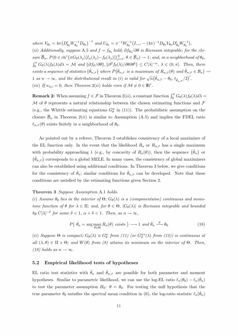
where Vθ0 = 4π(D′

θ0W−1

θ0Dθ0

)−1 and Uθ0 = π−1W−1θ0

(Ir×r − (4π)−1Dθ0Vθ0D

′θ0

W−1θ0

).

(ii) Additionally, suppose A.5 and f = fθ0 hold; ∂fθ0/∂θ is Riemann integrable; for the clo-

sure Bn, P (0 ∈ ch◦{πGθ(λj)[In(λj)−fθ(λj)]}Nj=1, θ ∈ Bn) → 1; and, in a neighborhood of θ0,∫ π

0 Gθ(λ)fθ(λ)dλ = M and ‖∂fθ/∂θ‖, ‖∂2fθ(λ)/∂θ∂θ′‖ ≤ C|λ|−α, λ ∈ (0, π]. Then, there

exists a sequence of statistics {θn,F} where P(θn,F is a maximum of Rn,F(θ) and θn,F ∈ Bn

) →1 as n →∞, and the distributional result in (i) is valid for

√n(θn,F − θ0, tθn,F

/2)′.

(iii) If κ4,ε = 0, then Theorem 2(ii) holds even if M 6= 0 ∈ IRr.

Remark 2: When assuming f ∈ F in Theorem 2(ii), a constant function∫ π0 Gθ(λ)fθ(λ)dλ =

M of θ represents a natural relationship between the chosen estimating functions and F(e.g., the Whittle estimating equations Gw

θ in (11)). The probabilistic assumption on the

closure Bn in Theorem 2(ii) is similar to Assumption (A.5) and implies the FDEL ratio

`n,F(θ) exists finitely in a neighborhood of θ0.

As pointed out by a referee, Theorem 2 establishes consistency of a local maximizer of

the EL function only. In the event that the likelihood Rn or Rn,F has a single maximum

with probability approaching 1 (e.g., by concavity of Rn(θ)), then the sequence {θn} or

{θn,F} corresponds to a global MELE. In many cases, the consistency of global maximizers

can also be established using additional conditions. In Theorem 3 below, we give conditions

for the consistency of θn; similar conditions for θn,F can be developed. Note that these

conditions are satisfied by the estimating functions given Section 2.

Theorem 3 Suppose Assumption A.1 holds.

(i) Assume θ0 lies in the interior of Θ; Gθ(λ) is a (componentwise) continuous and mono-

tone function of θ for λ ∈ Π; and, for θ ∈ Θ, |Gθ(λ)| is Riemann integrable and bounded

by C|λ|−δ for some δ < 1, α + δ < 1. Then, as n →∞,

P(

θn = arg maxθ∈Θ

Rn(θ) exists) −→ 1 and θn

p−→ θ0 (18)

(ii) Suppose Θ is compact; Gθ(λ) ≡ Gwθ from (11) (or Gw∗

ϑ (λ) from (12)) is continuous at

all (λ, θ) ∈ Π × Θ; and W (θ) from (8) attains its minimum on the interior of Θ. Then,

(18) holds as n →∞.

5.2 Empirical likelihood tests of hypotheses

EL ratio test statistics with θn and θn,F are possible for both parameter and moment

hypotheses. Similar to parametric likelihood, we can use the log-EL ratio `n(θ0) − `n(θn)

to test the parameter assumption H0: θ = θ0. For testing the null hypothesis that the

true parameter θ0 satisfies the spectral mean condition in (6), the log-ratio statistic `n(θn)

11

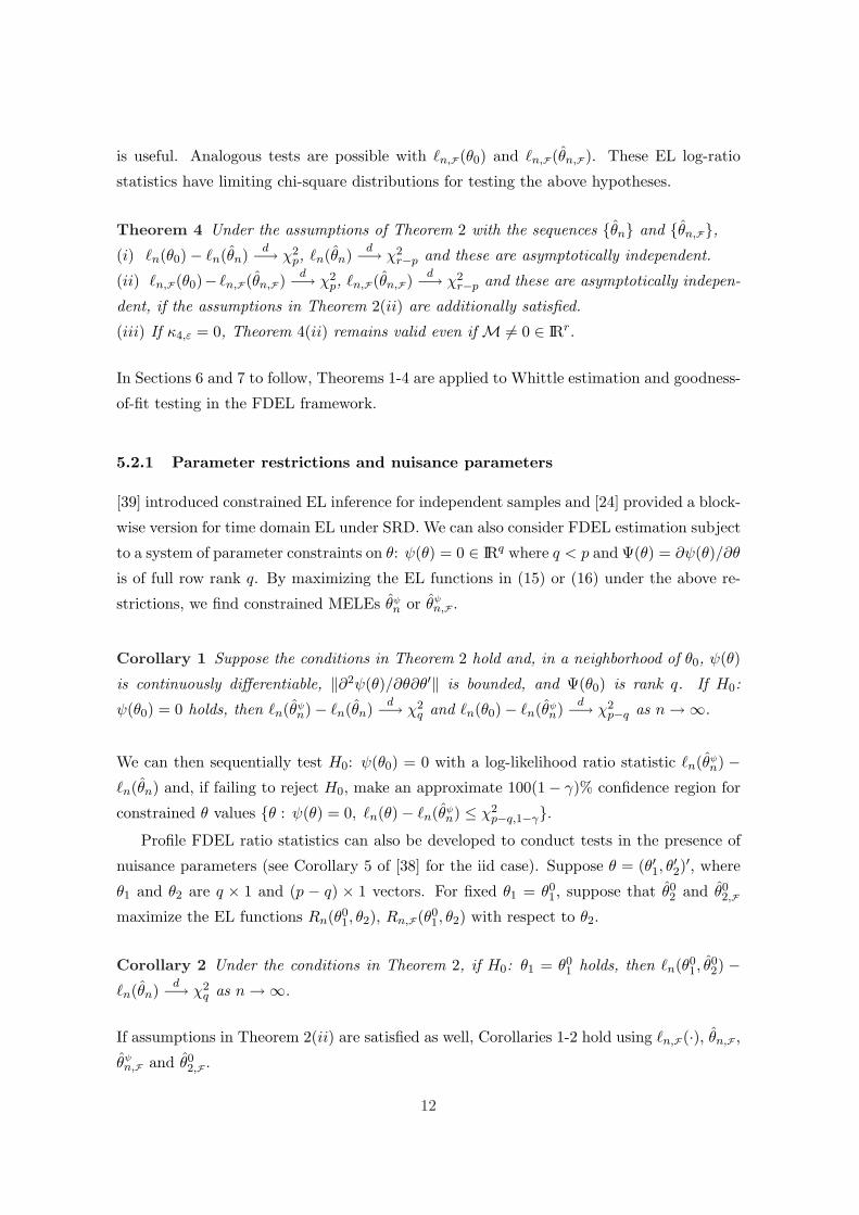
is useful. Analogous tests are possible with `n,F(θ0) and `n,F(θn,F). These EL log-ratio

statistics have limiting chi-square distributions for testing the above hypotheses.

Theorem 4 Under the assumptions of Theorem 2 with the sequences {θn} and {θn,F},(i) `n(θ0)− `n(θn) d−→ χ2

p, `n(θn) d−→ χ2r−p and these are asymptotically independent.

(ii) `n,F(θ0)− `n,F(θn,F) d−→ χ2p, `n,F(θn,F) d−→ χ2

r−p and these are asymptotically indepen-

dent, if the assumptions in Theorem 2(ii) are additionally satisfied.

(iii) If κ4,ε = 0, Theorem 4(ii) remains valid even if M 6= 0 ∈ IRr.

In Sections 6 and 7 to follow, Theorems 1-4 are applied to Whittle estimation and goodness-

of-fit testing in the FDEL framework.

5.2.1 Parameter restrictions and nuisance parameters

[39] introduced constrained EL inference for independent samples and [24] provided a block-

wise version for time domain EL under SRD. We can also consider FDEL estimation subject

to a system of parameter constraints on θ: ψ(θ) = 0 ∈ IRq where q < p and Ψ(θ) = ∂ψ(θ)/∂θ

is of full row rank q. By maximizing the EL functions in (15) or (16) under the above re-

strictions, we find constrained MELEs θψn or θψ

n,F .

Corollary 1 Suppose the conditions in Theorem 2 hold and, in a neighborhood of θ0, ψ(θ)

is continuously differentiable, ‖∂2ψ(θ)/∂θ∂θ′‖ is bounded, and Ψ(θ0) is rank q. If H0:

ψ(θ0) = 0 holds, then `n(θψn)− `n(θn) d−→ χ2

q and `n(θ0)− `n(θψn) d−→ χ2

p−q as n →∞.

We can then sequentially test H0: ψ(θ0) = 0 with a log-likelihood ratio statistic `n(θψn) −

`n(θn) and, if failing to reject H0, make an approximate 100(1− γ)% confidence region for

constrained θ values {θ : ψ(θ) = 0, `n(θ)− `n(θψn) ≤ χ2

p−q,1−γ}.Profile FDEL ratio statistics can also be developed to conduct tests in the presence of

nuisance parameters (see Corollary 5 of [38] for the iid case). Suppose θ = (θ′1, θ′2)′, where

θ1 and θ2 are q × 1 and (p − q) × 1 vectors. For fixed θ1 = θ01, suppose that θ0

2 and θ02,F

maximize the EL functions Rn(θ01, θ2), Rn,F(θ0

1, θ2) with respect to θ2.

Corollary 2 Under the conditions in Theorem 2, if H0: θ1 = θ01 holds, then `n(θ0

1, θ02) −

`n(θn) d−→ χ2q as n →∞.

If assumptions in Theorem 2(ii) are satisfied as well, Corollaries 1-2 hold using `n,F(·), θn,F ,

θψn,F and θ0

2,F .

12

6 Whittle estimation

Example 4 (continued). With SRD linear processes, [31] suggested EL confidence regions

for Whittle-like estimation of parameters θ = (σ2, ϑ′)′ characterizing fθ ∈ F from (9). The-

orem 1 provides two refinements to [31].

Refinement 1. [31] develops an EL function for θ by treating the standardized ordinates

In(λj)/fθ(λj), j = 1, . . . , N , as approximately iid random variables, similar to the FDB. The

EL ratio in (4.1) of [31] asymptotically corresponds to `n,F(θ) when using the estimating

functions Gwθ from (11). With this choice of functions, the non-zero spectral mean Mw 6= 0

in (11) is due to the first estimating function f−1θ intended to prescribe σ2. Note that the

use of `n,F(θ) and Gwθ for setting confidence regions requires the additional assumption that

the 4-th order innovation cumulant κ4,ε = 0 by Theorem 1. Valid joint confidence regions

are otherwise not possible here because Mw 6= 0. This complication due to σ2-inference is

related to the inconsistency of the FDB Whittle estimate of σ2 when κ4,ε 6= 0, as described

by [12]. While valid for SRD Gaussian series with κ4,ε = 0, periodogram-based EL formu-

lation in [31] may not be applicable to general SRD linear processes.

Refinement 2. Treating σ2 as a nuisance parameter and concentrating it out of the Whittle

likelihood, [31] suggests an EL ratio statistic for estimation of the remaining p− 1 parame-

ters ϑ in (9) via confidence regions. The statistic (6.1) of [31] appears to be asymptotically

equivalent to −2 log Rn(ϑ) = 1/2 · `n(ϑ) based on the p− 1 estimating functions Gw∗ϑ from

(12) and N = b(n− 1)/2c periodogram ordinates. Note that, for the function Gw∗ϑ , it holds

that Mw∗ = 0 so that Theorem 1(i) applies to `n(ϑ).

For Whittle-like estimation of ϑ in the parameterization from (9), the EL log-ratio

`n(ϑ) based on the functions Gw∗ϑ in (12) appears preferable to `n,F(ϑ). This selection

results in asymptotically correct confidence regions for ϑ under both SRD and LRD, even

for misspecified situations (f 6∈ F) where the moments in (10) still hold.

7 Goodness-of-fit tests

7.1 Simple hypothesis case

Example 3 (continued) We return to the simple hypothesis test H0: f = f0 for some

possible density f0. To assess the goodness-of-fit, [30] and [3] proposed the test statistic

Tn = πAn/B2n for mixing SRD linear processes (with κ4,ε = 0) and long-memory Gaussian

13

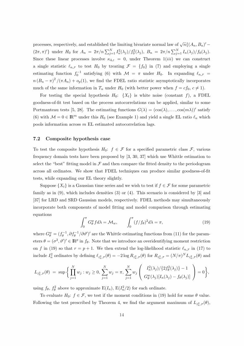
processes, respectively, and established the limiting bivariate normal law of√

n{(An, Bn)′−(2π, π)′} under H0 for An = 2π/n

∑Nj=1 I2

n(λj)/f20 (λj), Bn = 2π/n

∑Nj=1 In(λj)/f0(λj).

Since these linear processes involve κ4,ε = 0, under Theorem 1(iii) we can construct

a single statistic `n,F to test H0 by treating F = {f0} in (7) and employing a single

estimating function f−10 satisfying (6) with M = π under H0. In expanding `n,F =

n (Bn − π)2 /(πAn) + op(1), we find the FDEL ratio statistic asymptotically incorporates

much of the same information in Tn under H0 (with better power when f = cf0, c 6= 1).

For testing the special hypothesis H0: {Xt} is white noise (constant f), a FDEL

goodness-of-fit test based on the process autocorrelations can be applied, similar to some

Portmanteau tests [5, 28]. The estimating functions G(λ) = (cos(λ), . . . , cos(mλ))′ satisfy

(6) with M = 0 ∈ IRm under this H0 (see Example 1) and yield a single EL ratio `n which

pools information across m EL estimated autocorrelation lags.

7.2 Composite hypothesis case

To test the composite hypothesis H0: f ∈ F for a specified parametric class F , various

frequency domain tests have been proposed by [3, 30, 37] which use Whittle estimation to

select the “best” fitting model in F and then compare the fitted density to the periodogram

across all ordinates. We show that FDEL techniques can produce similar goodness-of-fit

tests, while expanding our EL theory slightly.

Suppose {Xt} is a Gaussian time series and we wish to test if f ∈ F for some parametric

family as in (9), which includes densities (3) or (4). This scenario is considered by [3] and

[37] for LRD and SRD Gaussian models, respectively. FDEL methods may simultaneously

incorporate both components of model fitting and model comparison through estimating

equations ∫ π

0Gw

θ fdλ = Mw,

∫ π

0(f/fθ)2dλ = π, (19)

where Gwθ = (f−1

θ , ∂f−1θ /∂ϑ′)′ are the Whittle estimating functions from (11) for the param-

eters θ = (σ2, ϑ′)′ ∈ IRp in fθ. Note that we introduce an overidentifying moment restriction

on f in (19) so that r = p + 1. We then extend the log-likelihood statistic `n,F in (17) to

include I2n ordinates by defining `I2

n,F(θ) = −2 log RI2n,F(θ) for RI2

n,F = (N/π)NLI2n,F(θ) and

LI2n,F(θ) = sup

{ N∏

j=1

wj : wj ≥ 0,N∑

j=1

wj = π,N∑

j=1

wj

I2

n(λj)/{2f2θ (λj)} − 1

Gwθ (λj)[In(λj)− fθ(λj)]

= 0

},

using fθ, f2θ above to approximate E(In), E(I2

n/2) for each ordinate.

To evaluate H0: f ∈ F , we test if the moment conditions in (19) hold for some θ value.

Following the test prescribed by Theorem 4, we find the argument maximum of LI2n,F(θ),

14

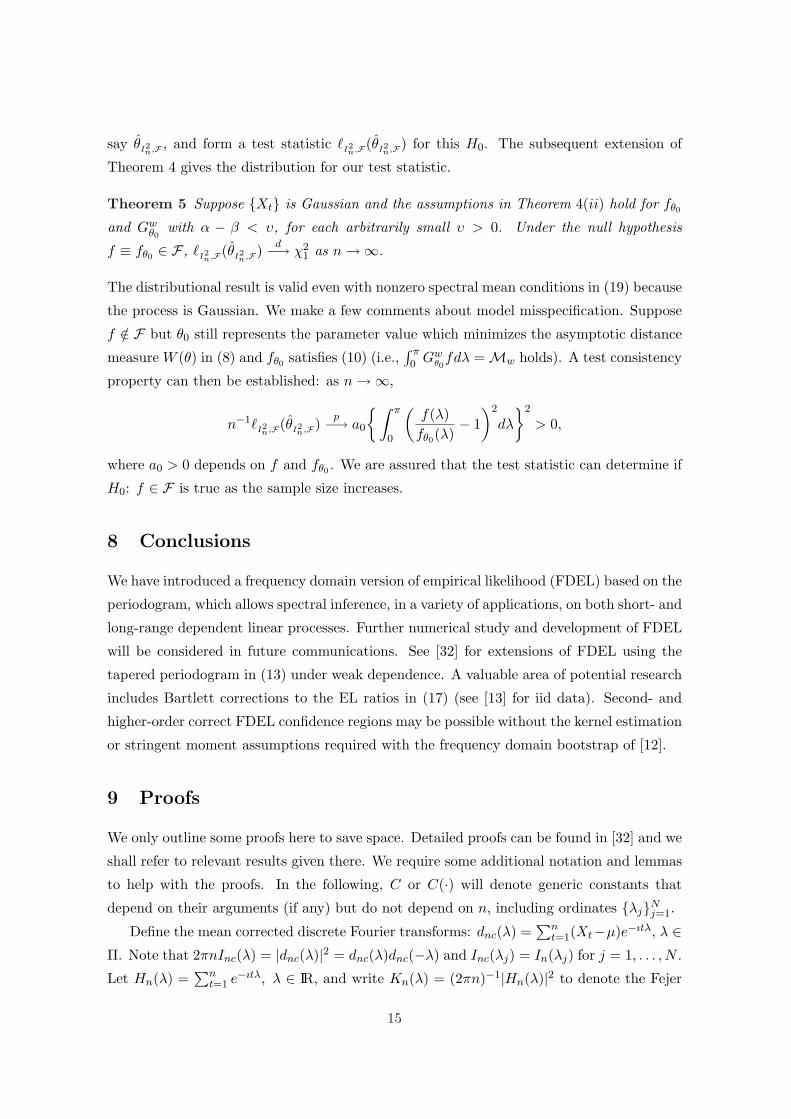
say θI2n,F , and form a test statistic `I2

n,F(θI2n,F) for this H0. The subsequent extension of

Theorem 4 gives the distribution for our test statistic.

Theorem 5 Suppose {Xt} is Gaussian and the assumptions in Theorem 4(ii) hold for fθ0

and Gwθ0

with α − β < υ, for each arbitrarily small υ > 0. Under the null hypothesis

f ≡ fθ0 ∈ F , `I2n,F(θI2

n,F) d−→ χ21 as n →∞.

The distributional result is valid even with nonzero spectral mean conditions in (19) because

the process is Gaussian. We make a few comments about model misspecification. Suppose

f /∈ F but θ0 still represents the parameter value which minimizes the asymptotic distance

measure W (θ) in (8) and fθ0 satisfies (10) (i.e.,∫ π0 Gw

θ0fdλ = Mw holds). A test consistency

property can then be established: as n →∞,

n−1`I2n,F(θI2

n,F)p−→ a0

{∫ π

0

(f(λ)

fθ0(λ)− 1

)2

dλ

}2

> 0,

where a0 > 0 depends on f and fθ0 . We are assured that the test statistic can determine if

H0: f ∈ F is true as the sample size increases.

8 Conclusions

We have introduced a frequency domain version of empirical likelihood (FDEL) based on the

periodogram, which allows spectral inference, in a variety of applications, on both short- and

long-range dependent linear processes. Further numerical study and development of FDEL

will be considered in future communications. See [32] for extensions of FDEL using the

tapered periodogram in (13) under weak dependence. A valuable area of potential research

includes Bartlett corrections to the EL ratios in (17) (see [13] for iid data). Second- and

higher-order correct FDEL confidence regions may be possible without the kernel estimation

or stringent moment assumptions required with the frequency domain bootstrap of [12].

9 Proofs

We only outline some proofs here to save space. Detailed proofs can be found in [32] and we

shall refer to relevant results given there. We require some additional notation and lemmas

to help with the proofs. In the following, C or C(·) will denote generic constants that

depend on their arguments (if any) but do not depend on n, including ordinates {λj}Nj=1.

Define the mean corrected discrete Fourier transforms: dnc(λ) =∑n

t=1(Xt−µ)e−ıtλ, λ ∈Π. Note that 2πnInc(λ) = |dnc(λ)|2 = dnc(λ)dnc(−λ) and Inc(λj) = In(λj) for j = 1, . . . , N .

Let Hn(λ) =∑n

t=1 e−ıtλ, λ ∈ IR, and write Kn(λ) = (2πn)−1|Hn(λ)|2 to denote the Fejer

15

kernel. The function Kn is nonnegative, even with period 2π on IR and∫Π Kn dλ = 1 (see

p. 71, [7]). We adopt the standard that an even function g : Π −→ IR can be periodically

(period 2π) extended to IR by g(λ) = g(−λ), g(λ) = g(λ+2π) for λ ∈ IR. We make extensive

use of the following function from [9]. Let Lns : IR −→ IR be the periodic extension of

Lns(λ) =:

e−sn |λ| ≤ es/n,logs(n|λ|)

|λ| es/n < |λ| ≤ π,λ ∈ Π, s = 0, 1.

For each n ≥ 1, s = 0, 1, Lns(·) is decreasing on [0, π] and

|Hn(λ)| ≤ C Ln0(λ), Ln0(λ) ≤ 3πn

1 + |λmod 2π|n, λ ∈ IR. (20)

In the following, cum(Y1, . . . , Ym) denotes the joint cumulant of random variables Y1, . . . , Ym.

We often refer to cumulant properties from Section 2.3 of [6], including the product theorem

for cumulants [c.f. Theorem 2.3.2].

We remark that Lemma 5 to follow ensures the log-likelihood ratio `n(θ0) exists asymp-

totically. Lemmas 6 and 7 establish important results for Riemann integrals based on the

periodogram under both LRD and SRD; Lemma 6 considers the distribution of empirical

spectral means and Lemma 7 is required for variance estimation.

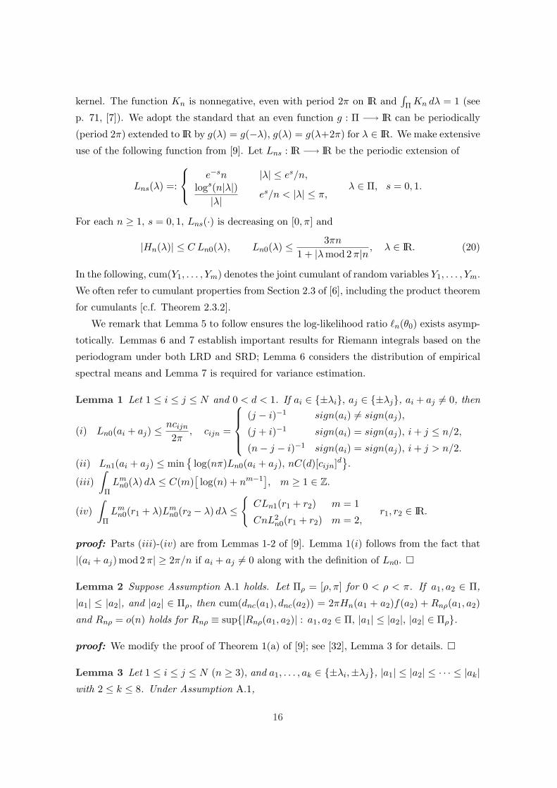
Lemma 1 Let 1 ≤ i ≤ j ≤ N and 0 < d < 1. If ai ∈ {±λi}, aj ∈ {±λj}, ai + aj 6= 0, then

(i) Ln0(ai + aj) ≤ ncijn

2π, cijn =

(j − i)−1 sign(ai) 6= sign(aj),

(j + i)−1 sign(ai) = sign(aj), i + j ≤ n/2,

(n− j − i)−1 sign(ai) = sign(aj), i + j > n/2.

(ii) Ln1(ai + aj) ≤ min{

log(nπ)Ln0(ai + aj), nC(d)[cijn]d}.

(iii)∫

ΠLm

n0(λ) dλ ≤ C(m)[log(n) + nm−1

], m ≥ 1 ∈ Z.

(iv)∫

ΠLm

n0(r1 + λ)Lmn0(r2 − λ) dλ ≤

{CLn1(r1 + r2) m = 1

CnL2n0(r1 + r2) m = 2,

r1, r2 ∈ IR.

proof: Parts (iii)-(iv) are from Lemmas 1-2 of [9]. Lemma 1(i) follows from the fact that

|(ai + aj)mod 2 π| ≥ 2π/n if ai + aj 6= 0 along with the definition of Ln0. ¤

Lemma 2 Suppose Assumption A.1 holds. Let Πρ = [ρ, π] for 0 < ρ < π. If a1, a2 ∈ Π,

|a1| ≤ |a2|, and |a2| ∈ Πρ, then cum(dnc(a1), dnc(a2)) = 2πHn(a1 + a2)f(a2) + Rnρ(a1, a2)

and Rnρ = o(n) holds for Rnρ ≡ sup{|Rnρ(a1, a2)| : a1, a2 ∈ Π, |a1| ≤ |a2|, |a2| ∈ Πρ}.

proof: We modify the proof of Theorem 1(a) of [9]; see [32], Lemma 3 for details. ¤

Lemma 3 Let 1 ≤ i ≤ j ≤ N (n ≥ 3), and a1, . . . , ak ∈ {±λi,±λj}, |a1| ≤ |a2| ≤ · · · ≤ |ak|with 2 ≤ k ≤ 8. Under Assumption A.1,

16

(i)∣∣∣cum

(dnc(a1), dnc(a2)

)∣∣∣ ≤ C

{|a1|−α

(|a2|−1 + Ln1(a1 + a2))

if α > 0,

Ln1(a1 + a2) if α = 0.

(ii)∣∣∣cum

(dnc(a1), . . . , dnc(ak)

)∣∣∣ ≤ C{|ak|α/2−1|ak−1|−1/2 + n logk−1(n)

} k∏

j=1

|aj |−α/2.

proof: We show Lemma 3(ii); the proof of (i) can be similarly shown with details given in

[32], Lemma 1. From [26, 41], the k-th order joint cumulant (2 ≤ k ≤ 8) may be expressed as:

cum(dnc(a1), . . . , dnc(ak)

)= (2π)−k+1κε,kν(Πk−1) using the k-th order innovation cumulant

κε,k and a function ν of Borel measurable sets A ⊂ Πk−1 defined as

ν(A) =∫

AHn

( k∑

j=1

aj −k−1∑

j=1

zj

)b

( k−1∑

j=1

aj − zj

) k−1∏

j=1

{Hn(zj)b(zj − aj)

}dz1, . . . , dzk−1.

On B =⋂k−1

j=1{(z1, . . . , zk−1) ∈ Πk−1 : |zj − aj | ≤ |aj |/2k}, we have |Hn(zj)| ≤ C|aj |−1,

|Hn(∑k

j=1 aj −∑k−1

j=1 zj)| ≤ C|ak|−1 by (20) and by applying Holder’s inequality

∫

|zk−1−ak−1|≤|ak−1|/2k

∣∣∣∣b( k−1∑

j=1

aj − zj

)b(zk−1 − ak−1)

∣∣∣∣dzk−1 ≤ C|ak−1|(1−α)/2

while∫|zj−aj |≤|aj |/2k|b(zj − aj)|dzj ≤ C|aj |1−α/2 for 1 ≤ j ≤ k − 2. By these inequalities,

|ν(B)| ≤ C|ak|−1|ak−1|−1/2∏k−1

j=1 |aj |−α/2. Now on Bj = {(z1, . . . , zk−1) ∈ Πk−1 : |zj−aj | >|aj |/2k} for fixed 1 ≤ j ≤ k − 1, we find |b(zj − aj)| ≤ C|aj |−α/2, |Hn(zj)| ≤ C n, and

∫

Π

∣∣∣∣Hn

( k∑

`=1

a` −k−1∑

`=1

z`

)b

( k−1∑

`=1

a` − z`

)∣∣∣∣ dzj

≤∫

|λ|≤|ak|/2

C|ak|−1|λ|−α/2 dλ +∫

|λ|>|ak|/2

C |ak|−α/2Ln0(ak − λ) dλ ≤ C |ak|−α/2 log(n)

by Lemma 1(iii) while∫Π |Hn(z`)||b(z` − a`)| dz` ≤ C |a`|−α/2 log(n) for each ` 6= j. Since

Πk−1 \ B =⋃k−1

j=1 Bj , we have |ν(Πk−1\B)| ≤ ∑k−1j=1 |ν(Bj)| ≤ Cn logk−1(n)

∏kj=1 |aj |−α/2.

¤

Lemma 4 Under Assumption A.1, r(k) = r(−k) = n−1∑n−k

j=1 (Xj − µ)(Xj+k − µ)p−→

r(k) = Cov(Xj , Xj+k) as n →∞ for each k ≥ 0.

proof: r(k) is asymptotically unbiased and Var(r(k)) = o(1) by Lemma 3.3 of [23]. ¤

Lemma 5 With Assumption A.1, suppose G = (g1, . . . , gr)′ ≡ Gθ0 is even with finite

discontinuities on [0, π] and satisfies Assumption A.2 and A.4. If∫Π Gfdλ = 0 ∈ IRr,

then P(0 ∈ ch◦

{πG(λj)In(λj)

}N

j=1

) → 1 as n →∞.

17

proof: See [32] for details. It can be shown that inf‖y‖=1

∫Π 11{y′G(λ)>0}y′Gf dλ ≥ C > 0

and that P (inf‖y‖=14πn

∑Nj=1 In(λj)y′G(λj) 11{y′G(λj)>0} ≥ C/2) → 1 follows using Lemma 4

with arguments from Lemma 1 of [21]. When the event in this probability statement holds,

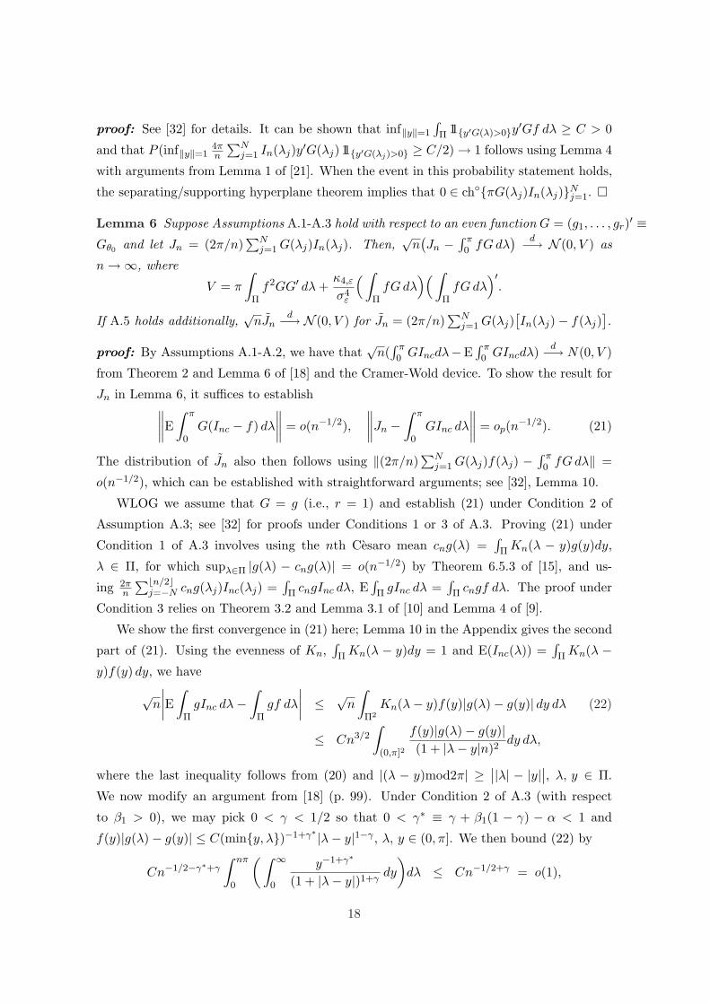
the separating/supporting hyperplane theorem implies that 0 ∈ ch◦{πG(λj)In(λj)}Nj=1. ¤

Lemma 6 Suppose Assumptions A.1-A.3 hold with respect to an even function G = (g1, . . . , gr)′ ≡Gθ0 and let Jn = (2π/n)

∑Nj=1 G(λj)In(λj). Then,

√n(Jn −

∫ π0 fG dλ

) d−→ N (0, V ) as

n →∞, where

V = π

∫

Πf2GG′ dλ +

κ4,ε

σ4ε

(∫

ΠfG dλ

)(∫

ΠfGdλ

)′.

If A.5 holds additionally,√

nJnd−→ N (0, V ) for Jn = (2π/n)

∑Nj=1 G(λj)

[In(λj)− f(λj)

].

proof: By Assumptions A.1-A.2, we have that√

n(∫ π0 GIncdλ−E

∫ π0 GIncdλ) d−→ N(0, V )

from Theorem 2 and Lemma 6 of [18] and the Cramer-Wold device. To show the result for

Jn in Lemma 6, it suffices to establish∥∥∥∥E

∫ π

0G(Inc − f) dλ

∥∥∥∥ = o(n−1/2),∥∥∥∥Jn −

∫ π

0GInc dλ

∥∥∥∥ = op(n−1/2). (21)

The distribution of Jn also then follows using ‖(2π/n)∑N

j=1 G(λj)f(λj) −∫ π0 fGdλ‖ =

o(n−1/2), which can be established with straightforward arguments; see [32], Lemma 10.

WLOG we assume that G = g (i.e., r = 1) and establish (21) under Condition 2 of

Assumption A.3; see [32] for proofs under Conditions 1 or 3 of A.3. Proving (21) under

Condition 1 of A.3 involves using the nth Cesaro mean cng(λ) =∫Π Kn(λ − y)g(y)dy,

λ ∈ Π, for which supλ∈Π |g(λ) − cng(λ)| = o(n−1/2) by Theorem 6.5.3 of [15], and us-

ing 2πn

∑bn/2cj=−N cng(λj)Inc(λj) =

∫Π cngInc dλ, E

∫Π gInc dλ =

∫Π cngf dλ. The proof under

Condition 3 relies on Theorem 3.2 and Lemma 3.1 of [10] and Lemma 4 of [9].

We show the first convergence in (21) here; Lemma 10 in the Appendix gives the second

part of (21). Using the evenness of Kn,∫Π Kn(λ − y)dy = 1 and E(Inc(λ)) =

∫Π Kn(λ −

y)f(y) dy, we have

√n

∣∣∣∣E∫

ΠgInc dλ−

∫

Πgf dλ

∣∣∣∣ ≤ √n

∫

Π2

Kn(λ− y)f(y)|g(λ)− g(y)| dy dλ (22)

≤ Cn3/2

∫

(0,π]2

f(y)|g(λ)− g(y)|(1 + |λ− y|n)2

dy dλ,

where the last inequality follows from (20) and |(λ − y)mod2π| ≥ ∣∣|λ| − |y|∣∣, λ, y ∈ Π.

We now modify an argument from [18] (p. 99). Under Condition 2 of A.3 (with respect

to β1 > 0), we may pick 0 < γ < 1/2 so that 0 < γ∗ ≡ γ + β1(1 − γ) − α < 1 and

f(y)|g(λ)− g(y)| ≤ C(min{y, λ})−1+γ∗ |λ− y|1−γ , λ, y ∈ (0, π]. We then bound (22) by

Cn−1/2−γ∗+γ

∫ nπ

0

(∫ ∞

0

y−1+γ∗

(1 + |λ− y|)1+γdy

)dλ ≤ Cn−1/2+γ = o(1),

18

using that there is a C > 0 where∫∞0 y−1+γ∗(1+ |λ−y|)−1−γdy ≤ C|λ|−1+γ∗ for any λ ∈ IR.

¤

Lemma 7 With Assumption A.1, suppose g and h are real-valued, even Riemann integrable

functions on Π such that |g(λ)|, |h(λ)| ≤ C|λ|β, 0 ≤ β < 1, α− β < 1/2. Then as n →∞,

2π

n

N∑

j=1

g(λj)h(λj)I2n(λj) and 2 · 2π

n

N∑

j=1

g(λj)h(λj)(In(λj)− f(λj))2p−→

∫

Πghf2 dλ.

proof: We consider the first Riemann sum above; convergence of the second sum can be

similarly established. Since (2π/n)∑N

j=1 g(λj)h(λj)f2(λj) →∫ π0 ghf2 dλ by the Lebesgue

Dominated Convergence Theorem, it suffices to establish

Bn ≡∣∣∣∣E(Sn)− 4π

n

N∑

j=1

g(λj)h(λj)f2(λj)∣∣∣∣ = o(1), Var(Sn) = o(1)

for Sn = (2π/n)∑N

j=1 g(λj)h(λj)I2n(λj). We show that Bn = o(1); Lemma 11 in the

Appendix shows Var(Sn) = o(1). By E(dnc(λ)) = 0 and the product theorem for cumulants,

(2πn)2E(I2n(λj)) = cum2

(dnc(λj), dnc(λj)

)+ 2 cum2

(dnc(λj), dnc(−λj)

)

+ cum(dnc(λj), dnc(λj), dnc(−λj), dnc(−λj)

). (23)

Then, Bn ≤ B1n + B2n + B3n for terms Bin defined in the following.

Using that n−12πLn0(2λj) ≤ (2j)−111{j≤bn/4c} + (n− 2j)−111{j>bn/4c} by Lemma 1 and

that cum(dnc(λj), dnc(λj)

) ≤ Cλ−αj (λ−1

j + log(n)Ln0(2λj)) by Lemma 3(i), we have for

B1n = n−3∑N

j=1 |g(λj)h(λj)|cum2(dnc(λj), dnc(λj)

)that

B1n ≤ C n−1+max{0,2α−2β} log2(n)( bn/4c∑

j=1

j−2 +N∑

j=bn/4c+1

(n− 2j)−2

)= o(1).

By Lemma 3(ii), |cum(dnc(λj), dnc(λj), dnc(−λj), dnc(−λj)

)| ≤ C n(n1/2+log3(n)

)λ−2α

j so

that B2n = n−3∑N

j=1

∣∣g(λj)h(λj)cum(dnc(λj), dnc(λj), dnc(−λj), dnc(−λj)

)∣∣ = o(1). Pick

0 < ρ < π. Using Lemma 3(i) and Lemma 2, for an arbitrarily small ρ we may bound

limB3n ≤ lim

C

n

∑

λ1≤λj<ρ

λ2β−2αj +

Rnρ

n· C

n

∑

ρ≤λj≤λN

λ2β−αj

≤ C

∫ ρ

0λ2β−2αdλ

for B3n =∣∣4π/n

∑Nj=1 g(λj)h(λj)[cumj − f(λj)][cumj + f(λj)]

∣∣, where we denote cumj =

cum(dnc(λj), dnc(−λj))/(2πn). As C does not depend on ρ above, B3n = o(1) follows. ¤

Lemma 8 Suppose Assumption A.1 holds and 0 ≤ β < 1, α − β < 1/2. Let ω =

max{1/3, 1/4 + (α− β)/2}. Then, max1≤j≤N In(λj)λβj = op(nω) and max1≤j≤N f(λj)λ

βj =

o(nω).

19

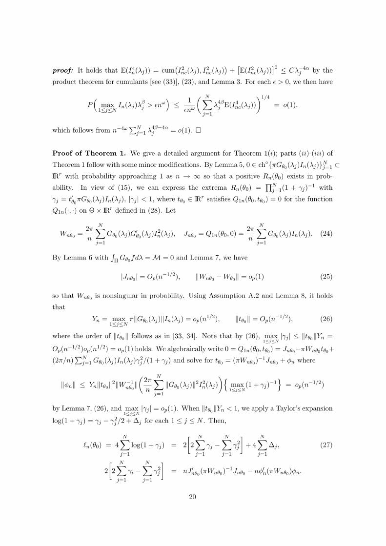
proof: It holds that E(I4n(λj)) = cum

(I2nc(λj), I2

nc(λj))

+[E(I2

nc(λj))]2 ≤ Cλ−4α

j by the

product theorem for cumulants [see (33)], (23), and Lemma 3. For each ε > 0, we then have

P(

max1≤j≤N

In(λj)λβj > εnω

)≤ 1

εnω

( N∑

j=1

λ4βj E(I4

nc(λj)))1/4

= o(1),

which follows from n−4ω∑N

j=1 λ4β−4αj = o(1). ¤

Proof of Theorem 1. We give a detailed argument for Theorem 1(i); parts (ii)-(iii) of

Theorem 1 follow with some minor modifications. By Lemma 5, 0 ∈ ch◦{πGθ0(λj)In(λj)}Nj=1 ⊂

IRr with probability approaching 1 as n → ∞ so that a positive Rn(θ0) exists in prob-

ability. In view of (15), we can express the extrema Rn(θ0) =∏N

j=1(1 + γj)−1 with

γj = t′θ0πGθ0(λj)In(λj), |γj | < 1, where tθ0 ∈ IRr satisfies Q1n(θ0, tθ0) = 0 for the function

Q1n(·, ·) on Θ× IRr defined in (28). Let

Wnθ0 =2π

n

N∑

j=1

Gθ0(λj)G′θ0

(λj)I2n(λj), Jnθ0 = Q1n(θ0, 0) =

2π

n

N∑

j=1

Gθ0(λj)In(λj). (24)

By Lemma 6 with∫Π Gθ0fdλ = M = 0 and Lemma 7, we have

|Jnθ0 | = Op(n−1/2), ‖Wnθ0 −Wθ0‖ = op(1) (25)

so that Wnθ0 is nonsingular in probability. Using Assumption A.2 and Lemma 8, it holds

that

Yn = max1≤j≤N

π‖Gθ0(λj)‖In(λj) = op(n1/2), ‖tθ0‖ = Op(n−1/2), (26)

where the order of ‖tθ0‖ follows as in [33, 34]. Note that by (26), max1≤j≤N

|γj | ≤ ‖tθ0‖Yn =

Op(n−1/2)op(n1/2) = op(1) holds. We algebraically write 0 = Q1n(θ0, tθ0) = Jnθ0−πWnθ0tθ0+

(2π/n)∑N

j=1 Gθ0(λj)In(λj)γ2j /(1 + γj) and solve for tθ0 = (πWnθ0)

−1Jnθ0 + φn where

‖φn‖ ≤ Yn‖tθ0‖2‖W−1nθ0‖(

2π

n

N∑

j=1

‖Gθ0(λj)‖2I2n(λj)

){max1≤j≤N

(1 + γj)−1}

= op(n−1/2)

by Lemma 7, (26), and max1≤j≤N

|γj | = op(1). When ‖tθ0‖Yn < 1, we apply a Taylor’s expansion

log(1 + γj) = γj − γ2j /2 + ∆j for each 1 ≤ j ≤ N . Then,

`n(θ0) = 4N∑

j=1

log(1 + γj) = 2[2

N∑

j=1

γj −N∑

j=1

γ2j

]+ 4

N∑

j=1

∆j , (27)

2[2

N∑

j=1

γi −N∑

j=1

γ2j

]= nJ ′nθ0

(πWnθ0)−1Jnθ0 − nφ′n(πWnθ0)φn.

20

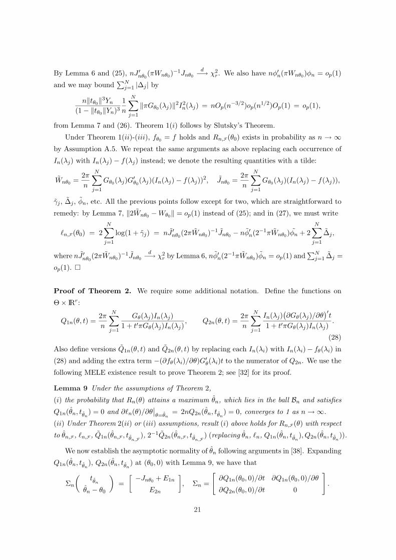
By Lemma 6 and (25), nJ ′nθ0(πWnθ0)

−1Jnθ0

d−→ χ2r . We also have nφ′n(πWnθ0)φn = op(1)

and we may bound∑N

j=1 |∆j | by

n‖tθ0‖3Yn

(1− ‖tθ0‖Yn)31n

N∑

j=1

‖πGθ0(λj)‖2I2n(λj) = nOp(n−3/2)op(n1/2)Op(1) = op(1),

from Lemma 7 and (26). Theorem 1(i) follows by Slutsky’s Theorem.

Under Theorem 1(ii)-(iii), fθ0 = f holds and Rn,F(θ0) exists in probability as n → ∞by Assumption A.5. We repeat the same arguments as above replacing each occurrence of

In(λj) with In(λj)− f(λj) instead; we denote the resulting quantities with a tilde:

Wnθ0 =2π

n

N∑

j=1

Gθ0(λj)G′θ0

(λj)(In(λj)− f(λj))2, Jnθ0 =2π

n

N∑

j=1

Gθ0(λj)(In(λj)− f(λj)),

γj , ∆j , φn, etc. All the previous points follow except for two, which are straightforward to

remedy: by Lemma 7, ‖2Wnθ0 −Wθ0‖ = op(1) instead of (25); and in (27), we must write

`n,F(θ0) = 2N∑

j=1

log(1 + γj) = nJ ′nθ0(2πWnθ0)

−1Jnθ0 − nφ′n(2−1πWnθ0)φn + 2N∑

j=1

∆j ,

where nJ ′nθ0(2πWnθ0)

−1Jnθ0

d−→ χ2r by Lemma 6, nφ′n(2−1πWnθ0)φn = op(1) and

∑Nj=1 ∆j =

op(1). ¤

Proof of Theorem 2. We require some additional notation. Define the functions on

Θ× IRr:

Q1n(θ, t) =2π

n

N∑

j=1

Gθ(λj)In(λj)1 + t′πGθ(λj)In(λj)

, Q2n(θ, t) =2π

n

N∑

j=1

In(λj)(∂Gθ(λj)/∂θ

)′t

1 + t′πGθ(λj)In(λj).

(28)

Also define versions Q1n(θ, t) and Q2n(θ, t) by replacing each In(λi) with In(λi)− fθ(λi) in

(28) and adding the extra term −(∂fθ(λi)/∂θ)G′θ(λi)t to the numerator of Q2n. We use the

following MELE existence result to prove Theorem 2; see [32] for its proof.

Lemma 9 Under the assumptions of Theorem 2,

(i) the probability that Rn(θ) attains a maximum θn, which lies in the ball Bn and satisfies

Q1n(θn, tθn) = 0 and ∂`n(θ)/∂θ

∣∣θ=θn

= 2nQ2n(θn, tθn) = 0, converges to 1 as n →∞.

(ii) Under Theorem 2(ii) or (iii) assumptions, result (i) above holds for Rn,F(θ) with respect

to θn,F , `n,F , Q1n(θn,F , tθn,F), 2−1Q2n(θn,F , tθn,F

) (replacing θn, `n, Q1n(θn, tθn), Q2n(θn, tθn

)).

We now establish the asymptotic normality of θn following arguments in [38]. Expanding

Q1n(θn, tθn), Q2n(θn, tθn

) at (θ0, 0) with Lemma 9, we have that

Σn

(tθn

θn − θ0

)=

[ −Jnθ0 + E1n

E2n

], Σn =

[∂Q1n(θ0, 0)/∂t ∂Q1n(θ0, 0)/∂θ

∂Q2n(θ0, 0)/∂t 0

].

21

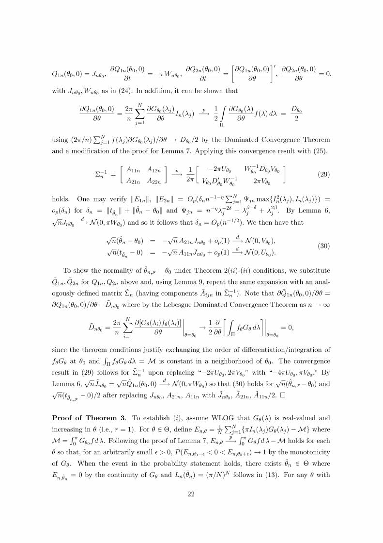
Q1n(θ0, 0) = Jnθ0 ,∂Q1n(θ0, 0)

∂t= −πWnθ0 ,

∂Q2n(θ0, 0)∂t

=[∂Q1n(θ0, 0)

∂θ

]′,

∂Q2n(θ0, 0)∂θ

= 0.

with Jnθ0 ,Wnθ0 as in (24). In addition, it can be shown that

∂Q1n(θ0, 0)∂θ

=2π

n

N∑

j=1

∂Gθ0(λj)∂θ

In(λj)p−→ 1

2

∫

Π

∂Gθ0(λ)∂θ

f(λ) dλ =Dθ0

2

using (2π/n)∑N

j=1 f(λj)∂Gθ0(λj)/∂θ → Dθ0/2 by the Dominated Convergence Theorem

and a modification of the proof for Lemma 7. Applying this convergence result with (25),

Σ−1n =

[A11n A12n

A21n A22n

]p−→ 1

2π

[ −2πUθ0 W−1θ0

Dθ0Vθ0

Vθ0D′θ0

W−1θ0

2πVθ0

](29)

holds. One may verify ‖E1n‖, ‖E2n‖ = Op(δnn−1−η∑N

j=1 Ψjn max{I2n(λj), In(λj)}) =

op(δn) for δn = ‖tθn‖ + ‖θn − θ0‖ and Ψjn = n−ηλ−2δ

j + λβ−δj + λ2β

j . By Lemma 6,√

nJnθ0

d−→ N (0, πWθ0) and so it follows that δn = Op(n−1/2). We then have that

√n(θn − θ0) = −√nA21nJnθ0 + op(1) d−→ N (0, Vθ0),√n(tθn

− 0) = −√nA11nJnθ0 + op(1) d−→ N (0, Uθ0).(30)

To show the normality of θn,F − θ0 under Theorem 2(ii)-(ii) conditions, we substitute

Q1n, Q2n for Q1n, Q2n above and, using Lemma 9, repeat the same expansion with an anal-

ogously defined matrix Σn (having components Aijn in Σ−1n ). Note that ∂Q1n(θ0, 0)/∂θ =

∂Q1n(θ0, 0)/∂θ− Dnθ0 where by the Lebesgue Dominated Convergence Theorem as n →∞

Dnθ0 =2π

n

N∑

i=1

∂[Gθ(λi)fθ(λi)]∂θ

∣∣∣∣θ=θ0

→ 12

∂

∂θ

[ ∫

ΠfθGθ dλ

]∣∣∣∣θ=θ0

= 0,

since the theorem conditions justify exchanging the order of differentiation/integration of

fθGθ at θ0 and∫Π fθGθ dλ = M is constant in a neighborhood of θ0. The convergence

result in (29) follows for Σ−1n upon replacing “−2πUθ0 , 2πVθ0” with “−4πUθ0 , πVθ0 .” By

Lemma 6,√

nJnθ0 =√

nQ1n(θ0, 0) d−→ N (0, πWθ0) so that (30) holds for√

n(θn,F−θ0) and√

n(tθn,F− 0)/2 after replacing Jnθ0 , A21n, A11n with Jnθ0 , A21n, A11n/2. ¤

Proof of Theorem 3. To establish (i), assume WLOG that Gθ(λ) is real-valued and

increasing in θ (i.e., r = 1). For θ ∈ Θ, define En,θ = 1N

∑Nj=1{πIn(λj)Gθ(λj)−M} where

M =∫ π0 Gθ0fd λ. Following the proof of Lemma 7, En,θ

p−→ ∫ π0 Gθfd λ−M holds for each

θ so that, for an arbitrarily small ε > 0, P (En,θ0−ε < 0 < En,θ0+ε) → 1 by the monotonicity

of Gθ. When the event in the probability statement holds, there exists θn ∈ Θ where

En,θn= 0 by the continuity of Gθ and Ln(θn) = (π/N)N follows in (13). For any θ with

22

|θ− θ0| ≥ ε, we have that En,θ 6= 0 implying Ln(θ) < Ln(θn). Hence, a global maximum θn

satisfies P (|θn − θ0| < ε) → 1.

For (ii), we consider Gθ ≡ Gwθ and M≡Mw from (11). Suppose θ∗n and θ∗ denote the

minimums of Wn(θ) = 14 log σ2

2π + 14πN

∑Nj=1 πIn(λj)f−1

θ (λj) and W (θ), respectively. Using

Lemma 4 with arguments as in Theorem 1 of [21], it follows that θ∗np−→ θ∗. Since θ∗ is inte-

rior to Θ, it holds that ∂Wn(θ∗n)/∂θ = 0, which implies En,θ∗n = 0 under the above definition

of En,θ with Gwθ ,Mw. Hence, Ln(θ∗n) = (π/N)N and, using Lemma 4 with arguments of

Lemma 1 of [21], 0 = En,θ∗np−→ ∫ π

0 Gθ∗fd λ−M holds whereby θ∗ = θ0 by uniqueness. We

then have a global maximum θn = θ∗n for which θnp−→ θ0. ¤

Proof of Theorem 4. Considering Theorem 4(i), let PX = X(X ′X)−1X ′ and Ir×r de-

note the projection matrix for a given matrix X and the r × r identity matrix. Writing

(πWθ0/n)1/2Znθ = Jnθ0 + Dθ0(θ − θ0)/2, it holds that |`(θn) − Z ′nθn

Znθn| = op(1) (see

Theorem 3, [32]) so that `n(θn) = Z ′nθ0(Ir×r − P

W−1/2θ0

Dθ0

)Znθ0 + op(1) using (29)-(30). By

(27), `n(θ0) = Z ′nθ0Znθ0 + op(1) where Znθ0

d−→ N (0, Ir×r) by Lemma 6. Theorem 4 follows

since PW−1/2θ0

Dθ0

, Ir×r−PW−1/2θ0

Dθ0

are orthogonal idempotent matrices with ranks p, r−p. ¤

Proofs of Corollaries 1 and 2. [32] gives a detailed proof of Corollary 1 and Corollary 2

follows by modifying arguments from Corollary 5 of [38]. ¤

Proof of Theorem 5. [32] provides details where the most important, additional distribu-

tional results required are (2π/√

n)∑N

j=1 Ynθ0,jd−→ N (0, πWθ0), (2π/n)

∑Nj=1 Ynθ0,jY

′nθ0,j

p−→Wθ0/2 for Ynθ0,j =

(I2nc(λj)/[2f2

θ0(λj)]− π, Inc(λj)Gw

θ0(λj)−Mw

)′ and

Wθ0 =

[W ∗

θ00

0 W ∗∗θ0

],W ∗

θ0=

[10π 4π

4π 2π

],W ∗∗

θ0=

(∫

Πf2

θ0

∂f−1θ0

∂ϑi

∂f−1θ0

∂ϑjdλ

)

i,j=1,...,p−1

.

The convergence results can be shown using arguments in [3] and [17]. ¤

10 Appendix

Lemma 10 Suppose Assumptions A.1-A.2 hold for a real-valued, even function g satisfying

Condition 2 of Assumption A.3. Define cng(λ) =∫Π Kn(λ − y)g(y) dy, λ ∈ Π, as the nth

Cesaro mean of the Fourier series of g and let Cn =∫ π0 cng(λ)Inc(λ)dλ. Then, as n →∞,

√n

∣∣∣∣ Cn −∫ π

0g(λ)Inc(λ) dλ

∣∣∣∣ = op(1),√

n

∣∣∣∣2π

n

N∑

j=1

g(λj)In(λj)− Cn

∣∣∣∣ = op(1). (31)

23

proof: Assume g satisfies A.1 and Condition 2 with respect to β and β1, respectively. We

establish the first part of (31). Using∫Π Kn(λ−y)dy = 1, E(Inc(λ)) =

∫Π Kn(λ−y)f(y) dy,

and Fubini’s Theorem, we write 2E| ∫ π0 (cng − g)Inc dλ| as

E∣∣∣∣∫

Π

Inc(λ)[ ∫

Π

Kn(λ− y)[g(y)− g(λ)] dy

]dλ

∣∣∣∣

≤∫

Π3

Kn(λ− z)Kn(λ− y)f(z)|g(y)− g(λ)| dz dy dλ ≤ t1n + t2n,

t1n =∫Π2 Kn(λ − z)f(z)|g(z) − g(λ)|dzdλ, t2n =

∫Π3 Kn(λ − z)Kn(y − λ)f(z)|g(y) −

g(z)|dλdzdy. It suffices to show√

n t2n = o(1) since arguments from (22) provide√

n t1n =

o(1). Applying Lemma 1(iv) and (20) sequentially, we bound∫Π Kn(λ− z)Kn(y−λ) dλ by

C

n2

∫

ΠL2

n0(λ− z)L2n0(y − λ) dλ ≤ C n

(1 + |(y − z)mod 2π|n)2.

From this and arguments from (22), we have

√n t2n ≤ Cn3/2

∫

Π2

f(z)|g(y)− g(z)|(1 + |(y − z)mod 2π|n)2

dzdy = o(1).

For the second part of (31), we use (2π/n)∑bn/2c

j=−N cng(λj)Inc(λj) = 2Cn and write

2√

n

∣∣∣∣2π

n

N∑

j=1

g(λj)In(λj)− Cn

∣∣∣∣ ≤ 4π√

n(t3n + t4n

),

t3n = n−1∑N

j=1 In(λj)|cng(λj) − g(λj)|, t4n = n−1(|cng(0)|Inc(0) + |cng(π)|Inc(π)). We

have√

nt4n = op(1) from E[Inc(0)] ≤ Cnα, |cng(0)| ≤ Cn−β and |cng(π)|E[Inc(π)] ≤ C by

Assumptions A.1-A.2. For a C > 0 independent of 1 ≤ j ≤ N (n > 3), if we establish

|cng(λj)− g(λj)| ≤ Cλβ1j

(log(n)

j+

11{j>n/4}n− 2j

), 1 ≤ j ≤ N, (32)

it will follow that√

nt3n ≤ Cn−1/2 log(n)(max1≤j≤N In(λj)λβ1j )

∑nj=1 j−1 = op(1) from

Lemma 8.

Fix 1 ≤ j ≤ N . To prove (32), we decompose the difference

|cng(λj)− g(λj)| =∣∣∣∣∫

ΠKn(y)[g(λj − y)− g(λj)] dy

∣∣∣∣ ≤∣∣∣∣∫ π

0d+

jn(y) dy

∣∣∣∣ +∣∣∣∣∫ π

0d−jn(y) dy

∣∣∣∣,

where d+jn(y) = Kn(y)[g(λj + y)− g(λj)], d−jn(y) = Kn(y)[g(λj − y)− g(λj)]. We separately

bound the last two absolute integrals using (20), |g(y) − g(z)| ≤ C |y|−1+β1 |z − y| for

24

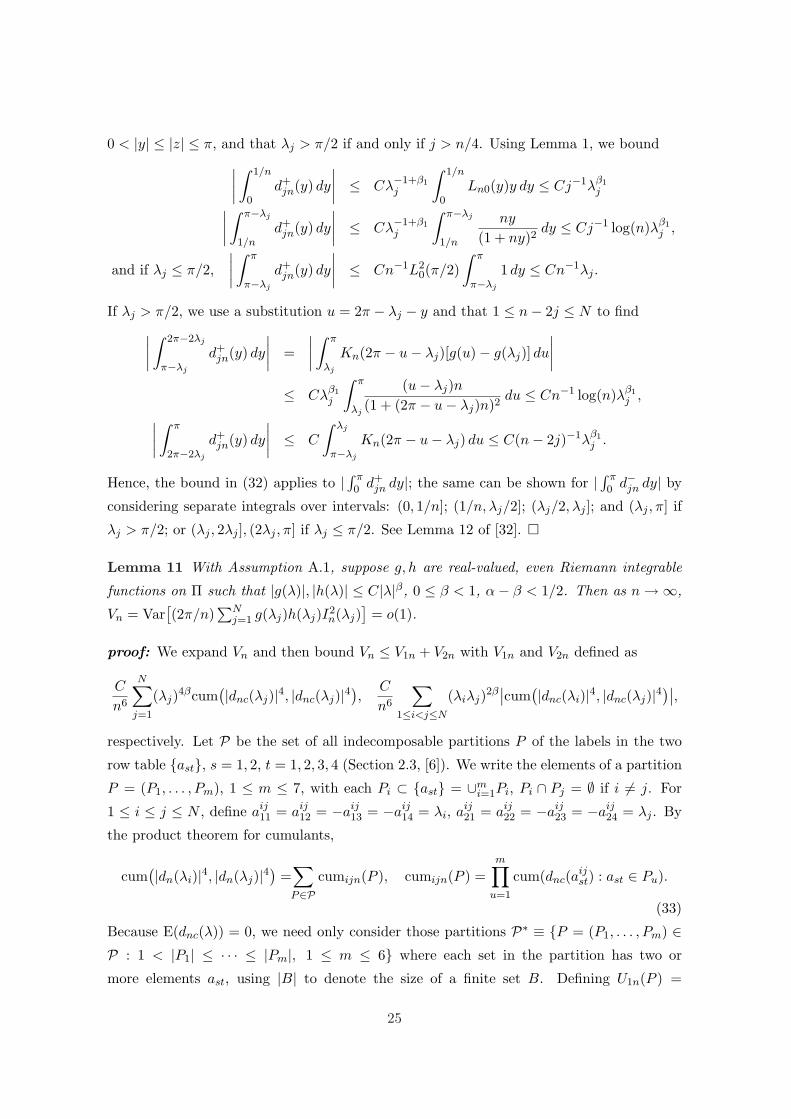
0 < |y| ≤ |z| ≤ π, and that λj > π/2 if and only if j > n/4. Using Lemma 1, we bound∣∣∣∣∫ 1/n

0d+

jn(y) dy

∣∣∣∣ ≤ Cλ−1+β1j

∫ 1/n

0Ln0(y)y dy ≤ Cj−1λβ1

j

∣∣∣∣∫ π−λj

1/nd+

jn(y) dy

∣∣∣∣ ≤ Cλ−1+β1j

∫ π−λj

1/n

ny

(1 + ny)2dy ≤ Cj−1 log(n)λβ1

j ,

and if λj ≤ π/2,∣∣∣∣∫ π

π−λj

d+jn(y) dy

∣∣∣∣ ≤ Cn−1L20(π/2)

∫ π

π−λj

1 dy ≤ Cn−1λj .

If λj > π/2, we use a substitution u = 2π − λj − y and that 1 ≤ n− 2j ≤ N to find∣∣∣∣∫ 2π−2λj

π−λj

d+jn(y) dy

∣∣∣∣ =∣∣∣∣∫ π

λj

Kn(2π − u− λj)[g(u)− g(λj)] du

∣∣∣∣

≤ Cλβ1j

∫ π

λj

(u− λj)n(1 + (2π − u− λj)n)2

du ≤ Cn−1 log(n)λβ1j ,

∣∣∣∣∫ π

2π−2λj

d+jn(y) dy

∣∣∣∣ ≤ C

∫ λj

π−λj

Kn(2π − u− λj) du ≤ C(n− 2j)−1λβ1j .

Hence, the bound in (32) applies to | ∫ π0 d+

jn dy|; the same can be shown for | ∫ π0 d−jn dy| by

considering separate integrals over intervals: (0, 1/n]; (1/n, λj/2]; (λj/2, λj ]; and (λj , π] if

λj > π/2; or (λj , 2λj ], (2λj , π] if λj ≤ π/2. See Lemma 12 of [32]. ¤

Lemma 11 With Assumption A.1, suppose g, h are real-valued, even Riemann integrable

functions on Π such that |g(λ)|, |h(λ)| ≤ C|λ|β, 0 ≤ β < 1, α− β < 1/2. Then as n →∞,

Vn = Var[(2π/n)

∑Nj=1 g(λj)h(λj)I2

n(λj)]

= o(1).

proof: We expand Vn and then bound Vn ≤ V1n + V2n with V1n and V2n defined as

C

n6

N∑

j=1

(λj)4βcum(|dnc(λj)|4, |dnc(λj)|4

),

C

n6

∑

1≤i<j≤N

(λiλj)2β∣∣cum

(|dnc(λi)|4, |dnc(λj)|4)∣∣,

respectively. Let P be the set of all indecomposable partitions P of the labels in the two

row table {ast}, s = 1, 2, t = 1, 2, 3, 4 (Section 2.3, [6]). We write the elements of a partition

P = (P1, . . . , Pm), 1 ≤ m ≤ 7, with each Pi ⊂ {ast} = ∪mi=1Pi, Pi ∩ Pj = ∅ if i 6= j. For

1 ≤ i ≤ j ≤ N , define aij11 = aij

12 = −aij13 = −aij

14 = λi, aij21 = aij

22 = −aij23 = −aij

24 = λj . By

the product theorem for cumulants,

cum(|dn(λi)|4, |dn(λj)|4

)=

∑

P∈Pcumijn(P ), cumijn(P ) =

m∏

u=1

cum(dnc(aijst) : ast ∈ Pu).

(33)

Because E(dnc(λ)) = 0, we need only consider those partitions P∗ ≡ {P = (P1, . . . , Pm) ∈P : 1 < |P1| ≤ · · · ≤ |Pm|, 1 ≤ m ≤ 6} where each set in the partition has two or

more elements ast, using |B| to denote the size of a finite set B. Defining U1n(P ) =

25

n−6∑N

j=1(λj)4β|cumjjn(P )| and U2n(P ) = n−6∑

1≤i<j≤N (λiλj)2β|cumijn(P )|, we can bound

Vin ≤ C∑

P∈P∗ Uin(P ), i = 1, 2, so that it suffices to show

Uin(P ) = o(1), P ∈ P∗, i = 1, 2. (34)

By Lemma 3, we have |cumjjn(P )| ≤ Cn4λ−4αj for P ∈ P∗, 1 ≤ j ≤ N so that U1n(P ) ≤

Cnmax{0,2α−2β}−1(n−1∑N

j=1 λ2β−2αj ) = o(1) since α − β < 1/2. Hence, (34) is established

for U1n and V1n = o(1).

We now show (34) for U2n(P ) by bounding |cumijn(P )|, over 1 ≤ i < j ≤ N , for several

cases of P = (P1, . . . , Pm) ∈ P∗. These cases are: m = 1; m = 2, |P2| = 6; m = 2,

|P2| = 5; m = 2, |P2| = 4; m = 3, |P3| = |P2| = 3; m = 3, |P3| = 4, |P2| = 2. The

last (seventh) case m = 4, |P1| = |P2| = |P3| = |P4| = 2 has the following subcases: (7.1)

there exist k1 6= k2 where∑

ast∈Pk1aij

st = 0 =∑

ast∈Pk2aij

st; (7.2) there exists exactly one

k where∑

ast∈Pkaij

st = 0; (7.3) for each k,∑

ast∈Pkaij

st 6= 0 holds and for some k1, k2,

|∑ast∈Pk1aij

st| = 2λi , |∑

ast∈Pk2aij

st| = 2λj ; (7.4) for each k, |∑ast∈Pkaij

st| 6∈ {0, 2λi, 2λj}.The first six cases follow from Lemma 3 and (20). For example, under cases 3 or 4, we

apply Lemma 3(ii) and (20) twice to bound |cumijn(P )| ≤ C{n3/2 + n log4(n)}2(λiλj)−2α

and then U2n(P ) ≤ Cn−1(n−1∑N

j=1 λ2β−2αj )2 = o(1). See Lemma 13 of [32] for details.

To treat case 7, we define some sets. For 0 < ρ < π/2, let A = {(i, j) : 1 ≤ i < j ≤ N},Aρ = {(i, j) ∈ A : λj < ρ}, Aρ = {(i, j) ∈ A : λj ≥ ρ}, An/2 = {(i, j) ∈ A : i + j > n/2} and

An/2 = {(i, j) ∈ A : i + j ≤ n/2}. We will also use that for integers j > i ≥ 1,

1i(j − i)

≤ 2j

if i = 1 or j(i− 1) > i2; otherwise,1i

<2j. (35)

For subcase 7.1, define Aρ1 = {(i, j) ∈ Aρ : i = 1 or j(i− 1) > i2} and Aρ2 = Aρ \Aρ1.

subcase 7.1: WLOG say k1 = 1, k2 = 2. We have |∑ast∈P3aij

st| = |∑ast∈P4aij

st| ∈{λj − λi, λj + λi} and, by Lemma 3(i),

∏2k=1 |cum(dnc(a

ijst) : ast ∈ Pk)| ≤ C n2(λiλj)−α.

Fix 0 < ρ < π/2. If |∑ast∈Pkaij

st| = λj − λi, k = 3, 4, then by Lemma 1(i), Lemma 2 and

(20) (for the sum involving λj ≥ ρ) or Lemma 1(i), Lemma 3(i) and (20) (for the sum with

λj < ρ):

U2n(P ) ≤ C(ρ)n4

∑

Aρ

λβ−αi

[n

j − i+ Rnρ

]2

+C

n4

∑

Aρ

λ2β−3αi λ2β−α

j

[λ−1

j +n

(j − i)d

]2

≡ u1n(ρ) + u2n(ρ),

u1n(ρ) ≤ C(ρ)(

n−1+max{0,α−β}n∑

j=1

j−2 + (n−1Rnρ)2(

1n

N∑

j=1

λβ−αj

))= o(1),

26

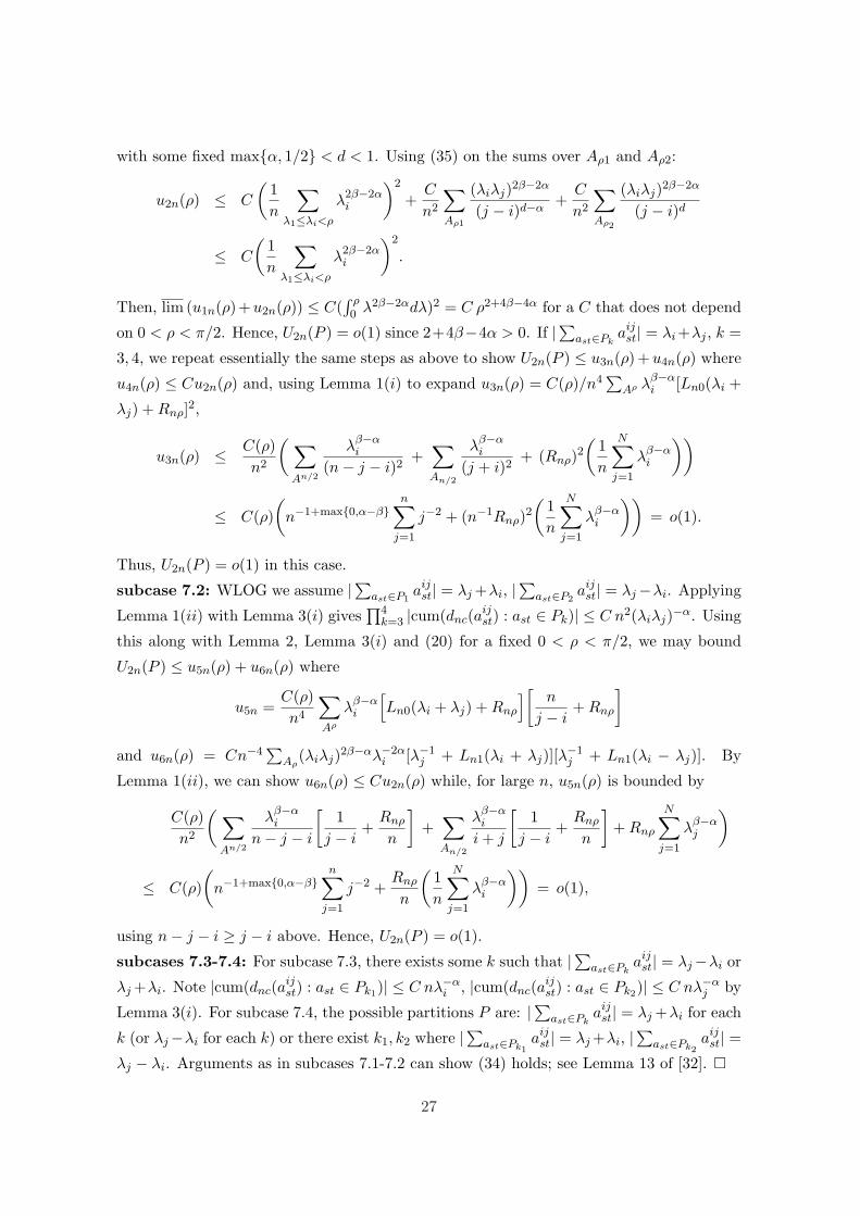
with some fixed max{α, 1/2} < d < 1. Using (35) on the sums over Aρ1 and Aρ2:

u2n(ρ) ≤ C

(1n

∑

λ1≤λi<ρ

λ2β−2αi

)2

+C

n2

∑

Aρ1

(λiλj)2β−2α

(j − i)d−α+

C

n2

∑

Aρ2

(λiλj)2β−2α

(j − i)d

≤ C

(1n

∑

λ1≤λi<ρ

λ2β−2αi

)2

.

Then, lim (u1n(ρ)+u2n(ρ)) ≤ C(∫ ρ0 λ2β−2αdλ)2 = C ρ2+4β−4α for a C that does not depend

on 0 < ρ < π/2. Hence, U2n(P ) = o(1) since 2+4β−4α > 0. If |∑ast∈Pkaij

st| = λi+λj , k =

3, 4, we repeat essentially the same steps as above to show U2n(P ) ≤ u3n(ρ)+u4n(ρ) where

u4n(ρ) ≤ Cu2n(ρ) and, using Lemma 1(i) to expand u3n(ρ) = C(ρ)/n4∑

Aρ λβ−αi [Ln0(λi +

λj) + Rnρ]2,

u3n(ρ) ≤ C(ρ)n2

( ∑

An/2

λβ−αi

(n− j − i)2+

∑

An/2

λβ−αi

(j + i)2+ (Rnρ)2

(1n

N∑

j=1

λβ−αi

))

≤ C(ρ)(

n−1+max{0,α−β}n∑

j=1

j−2 + (n−1Rnρ)2(

1n

N∑

j=1

λβ−αi

))= o(1).

Thus, U2n(P ) = o(1) in this case.

subcase 7.2: WLOG we assume |∑ast∈P1aij

st| = λj +λi, |∑

ast∈P2aij

st| = λj−λi. Applying

Lemma 1(ii) with Lemma 3(i) gives∏4

k=3 |cum(dnc(aijst) : ast ∈ Pk)| ≤ C n2(λiλj)−α. Using

this along with Lemma 2, Lemma 3(i) and (20) for a fixed 0 < ρ < π/2, we may bound

U2n(P ) ≤ u5n(ρ) + u6n(ρ) where

u5n =C(ρ)n4

∑

Aρ

λβ−αi

[Ln0(λi + λj) + Rnρ

][ n

j − i+ Rnρ

]

and u6n(ρ) = Cn−4∑

Aρ(λiλj)2β−αλ−2α

i [λ−1j + Ln1(λi + λj)][λ−1

j + Ln1(λi − λj)]. By

Lemma 1(ii), we can show u6n(ρ) ≤ Cu2n(ρ) while, for large n, u5n(ρ) is bounded by

C(ρ)n2

( ∑

An/2

λβ−αi

n− j − i

[1

j − i+

Rnρ

n

]+

∑

An/2

λβ−αi

i + j

[1

j − i+

Rnρ

n

]+ Rnρ

N∑

j=1

λβ−αj

)

≤ C(ρ)(

n−1+max{0,α−β}n∑

j=1

j−2 +Rnρ

n

(1n

N∑

j=1

λβ−αi

))= o(1),

using n− j − i ≥ j − i above. Hence, U2n(P ) = o(1).

subcases 7.3-7.4: For subcase 7.3, there exists some k such that |∑ast∈Pkaij

st| = λj−λi or

λj +λi. Note |cum(dnc(aijst) : ast ∈ Pk1)| ≤ C nλ−α

i , |cum(dnc(aijst) : ast ∈ Pk2)| ≤ C nλ−α

j by

Lemma 3(i). For subcase 7.4, the possible partitions P are: |∑ast∈Pkaij

st| = λj +λi for each

k (or λj−λi for each k) or there exist k1, k2 where |∑ast∈Pk1aij

st| = λj +λi, |∑

ast∈Pk2aij

st| =λj − λi. Arguments as in subcases 7.1-7.2 can show (34) holds; see Lemma 13 of [32]. ¤

27

Acknowledgments

The authors wish to thank two referees and an Associate Editor for many constructive

comments and suggestions that significantly improved an earlier draft of this paper.

References

[1] Adenstedt, R. K. (1974). On large-sample estimation for the mean of a stationary

sequence. Ann. Statist. 2 1095-1107.

[2] Anderson, T. W. (1993). Goodness of fit tests for spectral distributions. Ann. Statist.

21 830-847.

[3] Beran, J. (1992). A goodness-of-fit test for time series with long range dependence. J.

R. Stat. Soc. Ser. B 54 749-760.

[4] Beran, J. (1994). Statistical methods for long memory processes. Chapman & Hall,

London.

[5] Box, G. E. P. and Ljung, G. M. (1978). Lack of fit in time series models. Biometrika

65 297-303.

[6] Brillinger, D. R. (1981). Time series: data analysis and theory. Holden-Day, San Fran-

cisco.

[7] Brockwell, P. J. and Davis, R. A. (1991). Time series: theory and methods. Second

Edition, Springer, New York.

[8] Cramer, H. (1946) Mathematical methods of statistics. Princeton University Press, N.J.

[9] Dahlhaus, R. (1983). Spectral analysis with tapered data. J. Time Ser. Anal. 4 163-175.

[10] Dahlhaus, R. (1985). On the asymptotic distribution of Bartlett’s Up-statistic. J. Time

Ser. Anal. 6 213-227.

[11] Dahlhaus, R. (1989). Efficient parameter estimation for self-similar processes. Ann.

Statist. 17 1749-1766.

[12] Dahlhaus, R. and Janas, D. (1996). A frequency domain bootstrap for ratio statistics

in time series analysis. Ann. Statist. 24 1934-1963.

[13] DiCiccio, T. J., Hall, P. and Romano, J. P. (1991). Empirical likelihood is Bartlett-

correctable. Ann. Statist. 19 1053-1061.

28

[14] Dzhaparidze, K. (1986). Parameter estimation and hypothesis testing in spectral anal-

ysis of stationary time series. Springer-Verlag, New York.

[15] Edwards, R. E. (1979). Fourier series: a modern introduction. Springer-Verlag, New

York.

[16] Fox, R. and Taqqu, M. S. (1986). Large sample properties of parameter estimates for

strongly dependent stationary Gaussian time series. Ann. Statist. 14 517-532.

[17] Fox, R. and Taqqu, M. S. (1987). Central limit theorems for quadratic forms in random

variables having long range dependence. Probab. Theory Rel. Fields 14 213-240.

[18] Giraitis, L. and Surgailis, D. (1990). A central limit theorem for quadratic forms in

strongly dependent linear variables and its application to asymptotical normality of

Whittle’s estimate. Probab. Theory Related Fields 86 87-104.

[19] Granger, C. W. J. and Joyeux, R. (1980). An introduction to long-memory time series

models and fractional differencing. J. Time Ser. Anal. 1 15-29.

[20] Hall, P. and La Scala, B. (1990). Methodology and algorithms of empirical likelihood.

Internat. Statist. Rev. 58 109-127.

[21] Hannan, E. J. (1973). The asymptotic theory of linear time-series models. J. Appl.

Probab. 10 130-145.

[22] Hosking, J. R. M. (1981). Fractional differencing. Biometrika 68 165-176.

[23] Hosoya, Y. (1997). A limit theory for long-range dependence and statistical inference

on related models. Ann. Statist. 25 105-137.

[24] Kitamura, Y. (1997). Empirical likelihood methods with weakly dependent processes.

Ann. Statist. 25 2084-2102.

[25] Lahiri, S. N. (1993). On the moving block bootstrap under long range dependence.

Statist. Probab. Lett. 11 405-413.

[26] Lahiri, S. N. (2003). A necessary and sufficient condition for asymptotic independence

of discrete Fourier transforms under short- and long-range dependence. Ann. Statist.

31 613-641.

[27] Lahiri, S. N. (2003). Resampling methods for dependent data. Springer, New York.

[28] Li, W. K. and McLeod, A. I. (1986). Fractional time series differencing. Biometrika 73

217-221.

29

[29] Mandelbrot, B. B. and Van Ness, J. W. (1968). Fractional Brownian motions, fractional

noises and applications. SIAM Rev. 10 422-437.

[30] Milhoj, A. (1981). A test of fit in time series models. Biometrika 68 177-188.

[31] Monti, A. C. (1997). Empirical likelihood confidence regions in time series models.

Biometrika 84 395-405.

[32] Nordman, D. J. (2002). Frequency domain empirical likelihood for short- and long-

range dependent processes. Ph.D. Dissertation. Department of Statistics, Iowa State

University, Ames, IA.

[33] Owen, A. B. (1988). Empirical likelihood ratio confidence intervals for a single func-

tional. Biometrika 75 237-249.

[34] Owen, A. B. (1990). Empirical likelihood confidence regions. Ann. Statist. 18 90-120.

[35] Owen, A. B. (1991). Empirical likelihood for linear models. Ann. Statist. 19 1725-1747.

[36] Owen, A. B. (2001). Empirical likelihood. Chapman & Hall, London.

[37] Paparoditis, E. (2000). Spectral density based goodness-of-fit tests for time series mod-

els. Scand. J. Statist. 27 143176.

[38] Qin, J. and Lawless, J. (1994). Empirical likelihood and general estimating equations.

Ann. Statist. 22 300-325.

[39] Qin, J. and Lawless, J. (1995). Estimating equations, empirical likelihood and con-

straints on parameters. Canad. J. Statist. 23 145-159.

[40] Robinson, P.M. (1995). Gaussian semiparametric estimation of long range dependence.

Ann. Statist. 23 1630-1661.

[41] Yajima, Y. (1989). A central limit theorem of Fourier transforms of strongly dependent

stationary processes. J. Time Series Anal. 10 375-383.

[42] Whittle, P. (1953). Estimation and information in stationary time series. Ark. Mat. 2

423-434.

[43] Wilks, S. S. (1938). The large-sample distribution of the likelihood ratio for testing

composite hypotheses. Ann. Math. Statist. 9 60-62.

30