In All Likelihood, Deep Belief Is Not Enough

Lucas Theis, Sebastian Gerwinn, Fabian Sinz and Matthias BethgeWerner Reichardt Centre for Integrative Neuroscience

Bernstein Center for Computational NeuroscienceMax-Planck-Institute for Biological CyberneticsSpemannstraße 41, 72076 Tubingen, Germany

{lucas,sgerwinn,fabee,mbethge}@tuebingen.mpg.de

Abstract

Statistical models of natural stimuli provide an important tool for researchers inthe fields of machine learning and computational neuroscience. A canonical way toquantitatively assess and compare the performance of statistical models is given bythe likelihood. One class of statistical models which has recently gained increasingpopularity and has been applied to a variety of complex data are deep belief networks.Analyses of these models, however, have been typically limited to qualitative analysesbased on samples due to the computationally intractable nature of the model likelihood.Motivated by these circumstances, the present article provides a consistent estimatorfor the likelihood that is both computationally tractable and simple to apply in practice.Using this estimator, a deep belief network which has been suggested for the modelingof natural image patches is quantitatively investigated and compared to other models ofnatural image patches. Contrary to earlier claims based on qualitative results, theresults presented in this article provide evidence that the model under investigation isnot a particularly good model for natural images.

1 Introduction

Statistical models of naturally occurring stimuli constitute an important tool in machinelearning and computational neuroscience, among many other areas. In machine learning,they have been applied both to supervised and unsupervised problems, such as denoising(e.g., Lyu and Simoncelli, 2007), classification (e.g., Lee et al., 2009) or prediction (e.g.,Doretto et al., 2003). In computational neuroscience, statistical models have been usedto analyze the structure of natural images as part of the quest to understand the tasksfaced by the visual system of the brain (e.g., Lewicki and Doi, 2005; Olshausen and Field,1996). Other examples include generative statistical models studied to derive better modelsof perceptual learning. Underlying these approaches is the assumption that the low-levelareas of the brain adapt to the statistical structure of their sensory inputs and are lessconcerned with goals of behavior.

An important measure to assess the performance of a statistical model is the likelihoodwhich allows us to objectively compare the density estimation performance of different

1

arX

iv:1

011.

6086

v1 [

stat

.ML

] 2

8 N

ov 2

010

Figure 1: Left: Natural image patches sampled from the van Hateren dataset (van Haterenand van der Schaaf, 1998). Right: Filters learned by a deep belief network trainedon whitened image patches.

models. Given two model instances with the same prior probability and a test set of datasamples, the ratio of their likelihoods already tells us everything we need to know to decidewhich of the two models is more likely to have generated the dataset. Furthermore, fordensities p and p, the negative expected log-likelihood represents the cross-entropy (orexpected log-loss) term of the Kullback-Leibler (KL) divergence,

DKL[p||p] = −∑x

p(x) log p(x)−H[p],

which is always non-negative and zero if and only if p and p are identical. The main moti-vation for the KL-divergence stems from coding theory, where the cross-entropy representsthe coding cost of encoding samples drawn from p with a code that would be optimal forsamples drawn from p. Correspondingly, the KL-divergence represents the additional cod-ing cost created by using an optimal code which assumes the distribution of the samples tobe p instead of p. Finally, the likelihood allows us to directly examine the success of maxi-mum likelihood learning for different training settings. Unfortunately, for many interestingmodels, the likelihood is intractable to compute exactly.

One such class of models which has attracted a lot of attention in recent years is givenby deep belief networks. Deep belief networks are hierarchical generative models introducedby Hinton et al. (Hinton and Salakhutdinov, 2006) together with a greedy learning ruleas an approach to the long-standing challenge of training deep neural networks, that is,hierarchical neural networks with many layers. In supervised tasks, they have been shownto learn representations which can be successfully employed in classification tasks, suchas character recognition (Hinton et al., 2006a) and speech recognition (Mohamed et al.,2009). In unsupervised tasks, where the likelihood is particularly important, they havebeen applied to a wide variety of complex datasets, such as patches of natural images

2

(Osindero and Hinton, 2008; Ranzato et al., 2010; Ranzato and Hinton, 2010; Lee and Ng,2007), motion capture recordings (Taylor et al., 2007) and images of faces (Susskind et al.,2008).

When applied to natural images, deep belief networks have been shown to developbiologically plausible features (Lee and Ng, 2007) and samples from the model were shownto adhere to certain statistical regularities also found in natural images (Osindero andHinton, 2008). Examples of natural image patches and features learned by a deep beliefnetwork are presented in Figure 1.

In this article, after reviewing the relevant aspects of deep belief networks, we will de-rive a consistent estimator for its likelihood and demonstrate the estimator’s applicabilityin practice by evaluating a model trained on natural image patches. After a thoroughquantitative analysis, we will argue that the deep belief network under consideration isnot a particularly good model for estimating the density of small natural image patches,as it is outperformed with respect to the likelihood even by simple mixture models. Fur-thermore, we will show that adding layers to the network has only a small effect on theoverall performance of the model if each layer is trained well enough and will offer a possi-ble explanation for this observation by analyzing a best-case scenario of the greedy learningprocedure commonly used for training deep belief networks.

2 Models

In this chapter we will review the statistical models used in the remainder of this article.In particular, we will describe the restricted Boltzmann machine (RBM) and some of itsvariants which constitute the main building blocks for constructing deep belief networks(DBNs). Furthermore, we will discuss some of the models’ properties relevant for estimatingthe likelihood of DBNs. Readers familiar with DBNs might want to skip this section orskim it to get acquainted with the notation.

Throughout this article, the goal of applying statistical models is assumed to be theapproximation of a particular distribution of interest—often called the data distribution.We will denote this distribution by p.

2.1 Boltzmann Machines

A Boltzmann machine is a potentially fully connected undirected graphical model—or Markovrandom field—with binary random variables. Its probability mass function is a Boltzmanndistribution over 2k binary states s ∈ {0, 1}k which is defined in terms of an energy func-tion E,

q(s) =1

Zexp(−E(s)), Z =

∑s

exp(−E(s)), (1)

where E is given by

E(s) = −1

2s>Ws− b>s = −1

2

∑i,j

siwijsj −∑i

sibi (2)

3

x

y

(A) (B) (C)

Figure 2: Boltzmann machines with different constraints on their connectivity. Filled nodesdenote observed variables, unfilled nodes denote hidden variables. A: A fully con-nected latent-variable Boltzmann machine. B: A restricted Boltzmann machineforming a bipartite graph. C: A semi-restricted Boltzmann machine, which incontrast to RBMs also allows connections between the visible units.

and depends on a symmetric weight matrix W ∈ Rk×k with zeros on the diagonal, i.e.wii = 0 for all i = 1, ..., k, and bias terms b ∈ Rk. Z is called partition function and ensuresthe normalization of q. In the following, unnormalized distributions will be marked with anasterisk:

q∗(s) = Zq(s) = exp(−E(s)).

Samples from the Boltzmann distribution can be obtained via Gibbs sampling, which op-erates by conditionally sampling each univariate random variable until some convergencecriterion is reached. From definitions (1) and (2) it follows that the conditional probabilityof a unit i being on given the states of all other units sj 6=i is given by

q(si = 1 | sj 6=i) = g

∑j

wijsj + bi

,

where g(x) = 1/(1 + exp(−x)) is the sigmoidal logistic function. The Boltzmann machinecan be seen as a stochastic generalization of the binary Hopfield network, which is basedon the same energy function but updates its units deterministically using a step function,i.e. a unit is set to 1 if

∑j wijsi + bi > 0 and set to 0 otherwise. In the limit of increasingly

large weight magnitudes, the logistic function becomes a step function and the deterministicbehavior of the Hopfield network can be recovered with the Boltzmann machine (Hinton,2007).

Of particular interest for building DBNs are latent variable Boltzmann machines, that is,Boltzmann machines for which the states s are only partially observed (Figure 2). We willrefer to states of observed—or visible—random variables as x and to states of unobserved—or hidden—random variables as y, such that s can be written as s = (x, y).

Approximation of the data distribution p(x) with the model distribution q(x) via max-imum likelihood (ML) learning can be implemented by following the gradient of the modellog-likelihood. In Boltzmann machines, this gradient is conceptually simple yet computa-tionally very hard to evaluate. The gradient of the expected log-likelihood with respect to

4

some parameter θ of the energy function is (Salakhutdinov, 2009):

Ep(x)[∂

∂θlog q(x)

]= Eq(x,y)

[∂

∂θE(x, y)

]− Ep(x)q(y|x)

[∂

∂θE(x, y)

]. (3)

The first term on the right-hand side of this equation is the expected gradient of the energyfunction when both hidden and observed states are sampled from the model, while thesecond term is the expected gradient of the energy function when the hidden states aredrawn from the conditional distribution of the model, given a visible state drawn from thedata distribution. Following this gradient increases the energy of the states which are morelikely with respect to the model distribution and decreases the energy of the states whichare more likely with respect to the data distribution. Remember that by the definition ofthe model (1), states with higher energy are less likely than states with lower energy.

As an example, the gradient of the log-likelihood with respect to the weight connectinga visible unit xi and a hidden unit yj becomes

Ep(x)q(y|x)[xiyj ]− Eq(x,y)[xiyj ].

A step in the direction of this gradient can be interpreted as a combination of Hebbian andanti-Hebbian learning (Hinton, 2003), where the first term corresponds to Hebbian learningand the second term to anti-Hebbian learning, respectively.

Evaluating the expectations, however, is computationally intractable for all but thesimplest networks. Even approximating the expectations with Monte Carlo methods istypically very slow (Long and Servedio, 2010). Two measures can be taken to make learningin Boltzmann machines feasible: constraining the Boltzmann machine in some way, orreplacing the likelihood with a simpler objective function. The former approach led to theintroduction of RBMs, which will be discussed in the next section. The latter approachled to the now widely used contrastive divergence (CD) learning rule (Hinton, 2002) whichrepresents a tractable approximation to ML learning: In CD learning, the expectation overthe model distribution q(x, y) is replaced by an expectation over

qCD(x, y) =∑x0,y1

p(x0)q(y1 | x0)q(x | y1)q(y | x),

from which samples are obtained by taking a sample x0 from the data distribution, updatingthe hidden units, updating the visible units, and finally updating the hidden units again,while in each step keeping the respective set of other variables fixed. This correspondsto a single sweep of Gibbs sampling through all random variables of the model plus anadditional update of the hidden units. If instead n sweeps of Gibbs sampling are used, thelearning procedure is generally referred to as CD(n) learning. For n → ∞, ML learning isregained (Salakhutdinov, 2009).

2.2 Restricted Boltzmann Machines

A restricted Boltzmann machine (RBM) (Smolensky, 1986) is a Boltzmann machine whoseenergy function is constrained such that no direct interaction between two visible units ortwo hidden units is possible,

E(x, y) = −x>Wy − b>x− c>y.

5

The corresponding graph has no connections between the visible units and no connectionsbetween the hidden units and is hence bipartite (Figure 2). The weight matrix W ∈ Rm×nis different to the one in equation (2) in that it now only contains interaction terms betweenthe m visible units and the n hidden units and therefore no longer needs to be symmetric orconstrained in any other way. Despite these constraints it has been shown that RBMs areuniversal approximators, i.e. for any distribution over binary states and any ε > 0, thereexists an RBM with a KL-divergence which is smaller than ε (Roux and Bengio, 2008).

In an RBM, the visible units are conditionally independent given the states of the hiddenunits and vice versa. The conditional distribution of the hidden units, for instance, is givenby

q(y | x) =∏j

q(yj | x), q(yj | x) = g(w>j x+ cj),

where g is the logistic sigmoidal function and wj is the j-th column of W . This allowsfor efficient Gibbs sampling of the model distribution (since one set of variables can beupdated in parallel given the other) and thus for faster approximation of the log-likelihoodgradient. Moreover, the unnormalized marginal distributions q∗(x) and q∗(y) of RBMs canbe computed analytically by integrating out the respective other variable. For instance, theunnormalized marginal distribution of the visible units becomes

q∗(x) = exp(b>x)∏j

(1 + exp(w>j x+ cj)). (4)

Two other models which can be used for constructing DBNs are the Gaussian RBM (GRBM)(Salakhutdinov, 2009) and the semi-restricted Boltzmann machine (SRBM) (Osindero andHinton, 2008). The GRBM employs continuous instead of binary visible units (while keep-ing the hidden units binary) and can thus be used to model continuous data. Its energyfunction is given by

E(x, y) =1

2σ2||x− b||2 − 1

σx>Wy − c>y. (5)

A somewhat more general definition allows a different σ for each individual visible unit(Salakhutdinov, 2009). As for the binary Boltzmann machine, training of the GRBM pro-ceeds by following the gradient given in equation (3), or an approximation thereof. Itsproperties are similar to that of an RBM, except that its conditional distribution q(x | y)is a multivariate Gaussian distribution whose mean is determined by the hidden units,

q(x | y) = N (x;Wy + b, σI).

Each state of the hidden units encodes one mean. σ controls the variance of each Gaussianand is the same for all states of the hidden units. The GRBM can therefore be interpretedas a mixture of an exponential number of Gaussian distributions with fixed, isotropic co-variance and parameter sharing constraints.

In an SRBM, only the hidden units are constrained to have no direct connections to eachother while the visible units are unconstrained (Figure 2). Importantly, analytic expressionsare therefore only available for q∗(x) but not for q∗(y). Furthermore, q(x | y) is no longer

6

factorial. For efficiently training DBNs, conditional independence of the hidden units ismore important than conditional independence of the visible units (Osindero and Hinton,2008). This is in part due to the fact that the second-term on the right-hand side of equation(3) can still efficiently be evaluated if the hidden units are conditionally independent, andin part due to the way inference is done in DBNs.

2.3 Deep Belief Networks

x

y

z

Figure 3: A graphical model representation of a two-layer deep belief network composed oftwo RBMs. Note that the connections of the first layer are directed.

DBNs (Hinton and Salakhutdinov, 2006) are hierarchical generative models composedof several layers of RBMs or one of their generalizations. While DBNs have been widelyused as part of a heuristic for learning multiple layers of feature representations and forpretraining multi-layer perceptrons (by initializing the multi-layer perceptron with the pa-rameters learned by a DBN), the existence of an efficient learning rule has made thembecome attractive also for density estimation tasks.

For simplicity, we will begin by defining a two-layer DBN. Let q(x, y) and r(y, z) bethe densities of two RBMs over visible states x and hidden states y and z. Then, the jointprobability mass function of a two-layer DBN is defined to be

p(x, y, z) = q(x | y)r(y, z). (6)

Interestingly, the resulting distribution is best described not as a deep Boltzmann machine,as one might expect, or even an undirected graphical model, but as a graphical modelwith undirected connections between y and z and directed connections between x and y(Figure 3). This characteristic of the model becomes evident in the generative process. Asample from the model can be drawn by first Gibbs sampling the distribution r(y, z) of thetop layer to produce a state for y. Afterwards, a sample is drawn from the much simplerdistribution q(x | y).

The definition can easily be extended to DBNs with three or more layers by replacingr(y, z) = r(y | z)r(z) with r(y | z)s(z), where s(z) is the marginal distribution of anotherRBM. Thus, by adding additional layers to the DBN, the prior distribution over the top-levelhidden units—r(z) for the model defined in equation (6)—is effectively replaced with a newprior distribution—in this case s(z). DBNs with an arbitrary number of layers, like RBMs,have been shown to be universal approximators even if the number of hidden units in each

7

layer is fixed to the number of visible units (Sutskever and Hinton, 2008). As mentionedearlier, another possibility to generalize DBNs is to allow for more general models as layers.One such model is the SRBM, which can model more complex interactions by having lessrestrictive independce assumptions. Alternatively, one could allow for models with unitswhose conditional probability distributions are not just binary, but can be any exponentialfamily distribution (Welling et al., 2005)—one instance being the GRBM.

The greedy learning procedure (Hinton et al., 2006a) used for training DBNs starts byfitting the first-layer RBM (the one closest to the observations) to the data distribution.Afterwards, the prior distribution over the hidden units defined by the first layer, q(y) =∑

x q(x, y), is replaced by the marginal distribution of the second layer, r(y), and theparameters of the second layer are trained by optimizing a lower bound to the log-likelihoodof the two-layer DBN. In the following, we will derive this lower bound.

Let θ be a parameter of r. The gradient of the log-likelihood with respect to θ is

∂

∂θlog p(x) =

1

p(x)

∑y

∂

∂θp(x, y)

=1

p(x)

∑y

p(x, y)∂

∂θlog p(x, y)

=∑y

p(y | x)∂

∂θlog(r(y)q(x | y))

=∑y

p(y | x)

∂

∂θlog r(y) +

∂

∂θlog q(x | y)︸ ︷︷ ︸

= 0

=∑y

p(y | x)∂

∂θlog r(y). (7)

Approximate ML learning could therefore in principle be implemented by training the sec-ond layer to approximate the posterior distribution p(y | x) using CD learning or a similaralgorithm. However, exact sampling from the posterior distribution p(y | x) is difficult, asits evaluation involves integrating over an exponential number of states,

p(y | x) =p(x, y)

p(x)=

q(x | y)r(y)∑y q(x | y)r(y)

.

In order to make the training feasbile again, the posterior distribution is replaced by thefactorial distribution q(y | x). Training the DBN in this manner optimizes a variationallower bound on the log-likelihood,

log p(x) = log∑y

q(x | y)r(y)

= log∑y

q(y | x)q(x)

q(y)r(y) (8)

≥∑y

q(y | x) log r(y) + const, (9)

8

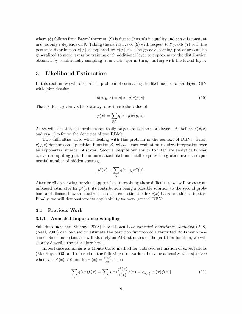
where (8) follows from Bayes’ theorem, (9) is due to Jensen’s inequality and const is constantin θ, as only r depends on θ. Taking the derivative of (9) with respect to θ yields (7) with theposterior distribution p(y | x) replaced by q(y | x). The greedy learning procedure can begeneralized to more layers by training each additional layer to approximate the distributionobtained by conditionally sampling from each layer in turn, starting with the lowest layer.

3 Likelihood Estimation

In this section, we will discuss the problem of estimating the likelihood of a two-layer DBNwith joint density

p(x, y, z) = q(x | y)r(y, z). (10)

That is, for a given visible state x, to estimate the value of

p(x) =∑y,z

q(x | y)r(y, z).

As we will see later, this problem can easily be generalized to more layers. As before, q(x, y)and r(y, z) refer to the densities of two RBMs.

Two difficulties arise when dealing with this problem in the context of DBNs. First,r(y, z) depends on a partition function Zr whose exact evaluation requires integration overan exponential number of states. Second, despite our ability to integrate analytically overz, even computing just the unnormalized likelihood still requires integration over an expo-nential number of hidden states y,

p∗(x) =∑y

q(x | y)r∗(y).

After briefly reviewing previous approaches to resolving these difficulties, we will propose anunbiased estimator for p∗(x), its contribution being a possible solution to the second prob-lem, and discuss how to construct a consistent estimator for p(x) based on this estimator.Finally, we will demonstrate its applicability to more general DBNs.

3.1 Previous Work

3.1.1 Annealed Importance Sampling

Salakhutdinov and Murray (2008) have shown how annealed importance sampling (AIS)(Neal, 2001) can be used to estimate the partition function of a restricted Boltzmann ma-chine. Since our estimator will also rely on AIS estimates of the partition function, we willshortly describe the procedure here.

Importance sampling is a Monte Carlo method for unbiased estimation of expectations(MacKay, 2003) and is based on the following observation: Let s be a density with s(x) > 0

whenever q∗(x) > 0 and let w(x) = q∗(x)s(x) , then

∑x

q∗(x)f(x) =∑x

s(x)q∗(x)

s(x)f(x) = Es(x) [w(x)f(x)] (11)

9

for any function f(x). s is called the proposal distribution and w(x) is called importanceweight. For f(x) = 1, we get

Es(x) [w(x)] =∑x

s(x)q∗(x)

s(x)= Zq. (12)

Estimates of the partition function Zq can therefore be obtained by drawing samples x(n)

from a proposal distribution and averaging the resulting importance weights w(x(n)). Itwas pointed out in (Minka, 2005) that minimizing the variance of the importance samplingestimate of the partition function (12) is equivalent to minimizing an α-divergence1 betweenthe proposal distribution s and the true distribution q. Therefore, for the estimate to workwell in practice, s should be both close to q and easy to sample from.

Annealed importance sampling (Neal, 2001) tries to circumvent some of the problemsassociated with finding a suitable proposal distribution. Assume we can construct a distri-bution s1 which approximates q well, but which is still difficult to sample from or which wecan only evaluate up to a normalization factor. Let s2 be another distribution. This distri-bution will effectively act as a proposal distribution for s1. Further, let T1 be a transitionoperator which leaves the distribution of s1 invariant, i.e. let T1(x0;x1) be a probabilitydistribution over x0 depending on x1, such that

s1(x0) =∑x1

s1(x1)T1(x0;x1).

We then have

Zq =∑x0

s1(x0)q∗(x0)

s1(x0)

=∑x0

∑x1

s1(x1)T1(x0;x1)q∗(x0)

s1(x0)

=∑x0

∑x1

s2(x1)T1(x0;x1)s∗1(x1)

s2(x1)

q∗(x0)

s∗1(x0).

Note that we don’t have to know the partition function of s1 to evaluate the right-handterm. Also note that we don’t need to sample from s1 but only from T1 if we want toestimate this term via Monte Carlo integration. If s2 is still too difficult to handle, we canapply the same trick again by introducing a third distribution s3 and a transition operatorT2 for s2. By induction, we can see that

Zq =∑x

sn(xn−1)Tn−1(xn−2;xn−1) · · ·T1(x0;x1)s∗n−1(xn−1)

sn(xn−1)· · · q

∗(x0)

s∗1(x0),

where the sum integrates over all x = (x0, ..., xn−1). Hence, in order to estimate the partitionfunction, we can draw independent samples xn−1 from a simple distribution sn, use thetransition operators to generate intermediate samples xn−2, ..., x0, and use the product offractions in the preceding equation to compute importance weights, which we then average.

1With α = 2. α-divergences are a generalization of the KL-divergence.

10

In order to be able to apply AIS to RBMs, a sequence of intermediate distributions andcorresponding annealing weights is defined:

s∗k(x) = q∗(x)1−βks(x)βk , βk ∈ [0, 1]

for k = 0, ..., n, where β0 = 0 and βn = 1. If we also choose an RBM for s, then sk is itselfa Boltzmann distribution whose energy function is a weighted sum of the energy functionsof s and q. Similarly, natural and efficient implementations based on Gibbs sampling canbe found for the transition operators Tk.

3.1.2 Estimating Lower Bounds

In (Salakhutdinov and Murray, 2008) it was also shown how estimates of a lower bound onthe log-likelihood,

log p(x) ≥∑y

q(y | x) logr∗(y)q(x | y)

q(y | x)− logZr (13)

=∑y

q(y | x) log r∗(y)q(x | y) +H[q(y | x)]− logZr, (14)

can be obtained, provided the partition function Zr is given. This is the same lower boundas the one optimized during greedy learning (9). Since q(y | x) is factorial, the entropyH[q(y | x)] can be computed analytically. The only term which still needs to be estimatedis the first term on the right-hand side of equation (14). This was achieved in (Salakhutdinovand Murray, 2008) by drawing samples from q(y | x).

3.1.3 Consistent Estimates

In (Murray and Salakhutdinov, 2009), carefully designed Markov chains were constructedto give unbiased estimates for the inverse posterior probability 1

p(y|x) of some fixed hidden

state y. These estimates were then used to get unbiased estimates of p∗(x) by taking

advantage of the fact p∗(x) = p∗(x,y)p(y|x) . The corresponding partition function was estimated

using AIS, leading to an overall estimate of the likelihood that tends to overestimate thetrue likelihood. While the estimator was constructed in such a way that even very shortruns of the Markov chain result in unbiased estimates of p∗(x), even a single step of theMarkov chain is slow compared to sampling from q(y | x) as it was done for the estimationof the lower bound (13).

3.2 A New Estimator for DBNs

The estimator we will introduce in this section shares the same formal properties as theestimator proposed in (Murray and Salakhutdinov, 2009), but will utilize samples drawnfrom q(y | x). This will make it conceptually as simple and as easy to apply in practice asthe estimator for the lower bound (13), while providing us with consistent estimates of p(x).

11

3.2.1 Definition

Let p(x, y, z) be the joint density of a DBN as defined in equation (10). By applying Bayes’theorem, we obtain

p(x) =∑y

q(x | y)r(y) (15)

=∑y

q(y | x)q(x)

q(y)r(y) (16)

=∑y

q(y | x)q∗(x)

q∗(y)

r∗(y)

Zr. (17)

An obvious choice for an estimator of p(x) is then

pN (x) =1

N

∑n

q∗(x)

q∗(y(n))

r∗(y(n))

Zr(18)

= q∗(x)1

ZrN

∑n

r∗(y(n))

q∗(y(n))(19)

where y(n) ∼ q(y(n) | x) for n = 1, ..., N . For RBMs, the unnormalized marginals q∗(x), q∗(y)and r∗(y) can be computed analytically (4). Note that the partition function Zr only hasto be calculated once for all visible states we wish to evaluate. Intuitively, the estimationprocess can be imagined as first assigning a basic value to x using the distribution of thefirst layer, and then with every sample adjusting this value depending on how the secondlayer distribution relates to the first layer distribution.

3.2.2 Properties

Under the assumption that the partition function Zr is known, p(x) provides an unbiasedestimate of p(x) since the sample average is always an unbiased estimate of the expectation.However, Zr is generally intractable to compute exactly so that approximations becomenecessary. In fact, in (Long and Servedio, 2010) it was shown that already approximatingthe partition function of an RBM to within a multiplicative factor is generally NP-hard inthe number of parameters of the RBM.

If in the estimate (18), Zr is replaced by an unbiased estimate Zr, then the overallestimate will tend to overestimate the true likelihood,

E[p∗N (x)

Zr

]= E

[1

Zr

]E [p∗N (x)]

≥ 1

E[Zr

]p∗(x) = p(x),

where p∗N (x) = ZrpN (x) is an unbiased estimate of the unnormalized density. The secondstep is a consequence of Jensen’s inequality and the averages are taken with respect to pN (x)and Zr, which are independent; x is held fix.

12

While the estimator loses its unbiasedness for unbiased estimates of the partition func-tion, it still retains its consistency. Since p∗N (x) is unbiased for all N ∈ N, it is alsoasymptotically unbiased,

plimN→∞

p∗N (x) = p∗(x).

Furthermore, if Zr,N for N ∈ N is a consistent sequence of estimators for the partitionfunction, it follows that

plimN→∞

p∗N (x)

Zr,N=

plimN→∞

p∗N (x)

plimN→∞

Zr,N=p∗(x)

Zr= p(x).

Unbiased and consistent estimates of Zr can be obtained using AIS (Salakhutdinov andMurray, 2008). Note that although the estimator tends to overestimate the true likelihoodin expectation and is unbiased in the limit, it is still possible for it to underestimate thetrue likelihood most of the time. This behavior can occur if the distribution of estimates isheavily skewed.

Another question which remains is whether the estimator is good in terms of efficiency,or in other words: How many samples are required before a reliable estimate of the truelikelihood is achieved? To address this question, we reformulate the expectation in equation(17) to give

p(x) =∑y

q(y | x)p(x, y)

q(y | x).

In this formulation it becomes evident that estimating p(x) is equivalent to estimating thepartition function of p(y | x) using importance sampling. To see this, notice that, for afixed x, p(x, y) is just an unnormalized version of p(y | x), where p(x) is the normalizationconstant,

p(y | x) =p(x, y)

p(x).

The proposal distribution in this case is q(y | x). As mentioned earlier, the efficiency ofimportance sampling estimates depends on how well the proposal distribution approximatesthe true distribution. Therefore, for the proposed estimator to work well in practice, q(y | x)should be close to p(y | x). Note that a similar assumption is made when optimizing thevariational lower bound (9) during greedy learning.

3.2.3 Generalizations

The definition of the estimator for two-layer DBNs readily extends to DBNs with L layers. Ifp(x) is the marginal density of a DBN whose layers are constituted by RBMs with densitiesq1, ..., qL and partition functions Z1, ..., ZL, and if we refer to the states of the random

13

vectors in each layer by x0, ..., xL, where x0 contains the visible states and xL contains thestates of the top hidden layer, then

p(x0) =∑

x1,...,xL−1

qL(xL−1)

L−1∏l=1

ql(xl−1 | xl)

=∑

x1,...,xL−1

qL(xL−1)L−1∏l=1

ql(xl | xl−1)q∗l (xl−1)

q∗l (xl)

= q∗1(x0)1

ZL

∑x1,...,xL−1

L−1∏l=1

ql(xl | xl−1)q∗l+1(xl)

q∗l (xl).

In order to estimate this term, hidden states x1, ..., xL are generated in a feed-forward

manner using the conditional distributions ql(xl | xl−1). The weightsq∗l+1(xl)

q∗l (xl)are computed

along the way, then multiplied together and finally averaged over all drawn states.

Often, a DBN not only contains RBMs but also more general distributions q(x, y) (see,for example, Roux et al., 2010; Osindero and Hinton, 2008; Ranzato et al., 2010; Ranzatoand Hinton, 2010). In this case, analytical expressions of the unnormalized distributionover the hidden states q∗(y) might be unavailable, as, for example, for the SRBM. If AIS orsome other importance sampling method is used for the estimation of the partition function,however, the same importance samples and importance weights can be used in order to getunbiased estimates of q∗(y), as we will show in the following.

As in equation (11), let s be a proposal distribution and w be importance weights suchthat ∑

x

s(x)w(x)f(x) =∑x

q∗(x)f(x).

for any function f . By noticing that q∗(y) =∑

x q∗(x)q(y | x), it easy to see how estimates

of q∗(y) can be obtained using the same importance samples and importance weights whichare used for estimating the partition function,

q∗(y) ≈ 1

N

∑n

w(n)q(y | x(n)).

As for the partition function, the importance weights only have to be generated once for allx and all hidden states that are part of the evaluation. Estimating q∗(y) in this manner,however, introduces further bias into the estimator. Also note that a good proposal distri-bution for estimating the partition function need not be a good proposal distribution forestimating the marginals. The optimal proposal distribution for estimating the marginalswould be q(x), as in this case any importance weight would take on the value of the partitionfunction itself (12). The optimal proposal distribution for estimating the value of the un-normalized marginal distribution q∗(y), on the other hand, is q(x | y), which unfortunatelydepends on y. Therefore, more importance samples will be needed in order to get reliableestimates of the marginals.

14

3.3 Potential Log-Likelihood

In this section, we will discuss the concept of the potential log-likelihood—a concept whichappears in (Roux and Bengio, 2008). By considering a best-case scenario, the potentiallog-likelihood gives an idea of the log-likelihood that can at best be achieved by trainingadditional layers using greedy learning. Its usefulness will become apparent in the experi-mental section.

Let q(x, y) be the distribution of an already trained RBM or one of its generalizations,and let r(y) be a second distribution—not necessarily the marginal distribution of any Boltz-mann machine. As in section 2.3, r(y) serves to replace the prior distribution over the hiddenvariables, q(y), and thereby improve the marginal distribution over x,

∑y q(x | y)r(y). As

above, let p(x) denote the data distribution. Our goal, then, is to increase the expectedlog-likelihood of the model distribution with respect to r,∑

x

p(x) log∑y

q(x | y)r(y). (20)

In applying the greedy learning procedure, we try to reach this goal by optimizing a lowerbound on the log-likelihood (9), or equivalently, by minimizing the following KL-divergence:

DKL

[∑x

p(x)q(y | x)||r(y)

]= −

∑x

p(x)∑y

q(y | x) log r(y) + const,

where const is constant in r.The KL divergence is minimal if r(y) is equal to∑

x

p(x)q(y | x) (21)

for every y. Since RBMs are universal approximators (Roux and Bengio, 2008), this dis-tribution could in principle be approximated arbitrarily well by a single, potentially verylarge RBM (provided the y are binary).

Assume that we have found this distribution, that is, we have maximized the lowerbound with respect to all possible distributions r. The distribution for the DBN which weobtain by replacing r in (20) with (21) is then given by∑

y

q(x | y)∑x0

p(x0)q(y | x0) =∑x0

p(x0)∑y

q(x | y)q(y | x0)

=∑x0

p(x0)q0(x | x0),

where we have used the reconstruction distribution

q0(x | x0) =∑y

q(x | y)q(y | x0),

which can be sampled from by conditionally sampling a state for the hidden units, and then,given the state of the hidden units, conditionally sampling a reconstruction of the visible

15

1

23

space of distributions r

[bit

s]

log-likelihoodlower bound

Figure 4: A cartoon explaining the potential log-likelihood. The potential log-likelihood isthe log-likelihood evaluated at (2), where the lower bound reaches its optimum (1).This does not exclude the existence of a distribution r for which the log-likelihoodis larger than the potential log-likelihood, as in (3), but it is unlikely that thispoint will be found by greedy learning, which optimizes r only with respect tothe lower bound.

units. The log-likelihood we achieve with this lower-bound optimal distribution is given by∑x

p(x) log∑x0

p(x0)q0(x | x0). (22)

we will refer to this log-likelihood as the potential log-likelihood (and to the correspondinglog-loss as the potential log-loss). Note that the potential log-likelihood is not a true upperbound on the log-likelihood that can be achieved with greedy learning, as suboptimal solu-tions with respect to the lower bound might still give rise to higher log-likelihoods. However,if such a solution was found, it would have rather been by accident than by design. Thesituation is depicted in the cartoon in Figure 4.

4 Experiments

In order to test the estimator, we considered the task of modeling 4x4 natural image patchessampled from the van Hateren dataset (van Hateren and van der Schaaf, 1998). We chose asmall patch size to allow for a more thorough analysis of the estimator’s behavior and theeffects of certain model parameters. In all experiments, a standard battery of preprocessingsteps was applied to the image patches, including a log-transformation, a centering step anda whitening step. Additionally, the DC component was projected out and only the other15 components of each image patch were used for training (for details, see Eichhorn et al.,2009).

In (Osindero and Hinton, 2008), a three-layer DBN based on GRBMs and SRBMs wassuggested for the modeling of natural image patches. The model employed a GRBM in the

16

layers true avg. log-loss est. avg. log-loss

1 2.0550777 2.05512892 2.0550775 2.05507343 2.0550773 2.0544256

Table 1: True and estimated log-loss of a small-scale version of the model. Adding morelayers to the network does not help to improve the performance if the GRBMemploys only few hidden units.

first layer and SRBMs in the second and third layer. In contrast to samples from the samemodel without lateral connections, samples from the proposed model were shown to possesssome of the statistical regularities also found in natural images, such as sparse distributionsof pixel intensities and the right pair-wise statistics of Gabor filter responses. Furthermore,the first layer of the model was shown to develop oriented edge filters (Figure 1). In thefollowing, we will further analyse this type of model by estimating its likelihood.

For training and evaluation, we used 10 independent pairs of training and test sets con-taining 50000 samples each. We trained the models using the greedy learning proceduredescribed in Section 2.3. The scale-parameter σ of the GRBM (5) was chosen via cross-validation. After training a GRBM, we initialized the second-layer SRBM such that itsvisible marginal distribution is equal to the hidden marginal distribution of the GRBM.Initializing the second layer in this manner has the following advantages. First, after ini-tialization, the likelihood of the two-layer DBN consisting of the trained GRBM and theinitialized SRBM is equal to the likelihood of the GRBM. Second, the lower bound on theDBN’s log-likelihood (9) is equal to its actual log-likelihood. Using the notation of theprevious sections:

r(y) = q(y)⇒∑y

q(y | x) log

(r(y)

q(x)

q(y)

)= log p(x).

As a consequence, an improvement in the lower bound necessarily leads to an improvementin the log-likelihood (Salakhutdinov, 2009).

All trained models were evaluated using the proposed estimator. We used AIS in orderto estimate the partition functions and the marginals of the SRBMs. Performances weremeasured as average log-loss in bits and normalized by the number of components. Detailson the training and evaluation parameters can be found in Appendix A.

4.1 Small Scale Experiment

In a first experiment, we investigated a small-scale version of the model for which thelikelihood is still tractable. It employed 15 hidden units in the first layer, 15 hidden unitsin the second layer and 50 hidden units in the third layer, where each layer was trained for50 epochs using CD(1). Brute-force and estimated results are given in Table 1.

A first observation which can be made is that the estimated performance is very closeto the true performance. Another observation is that the second and third layer do nothelp to improve the performance of the model, which hints at the fact that the 15 hidden

17

100 101 102 1030

0.5

1

1.5

2

number of AIS samples

log-

loss

[bit

s]

estimating marginalsestimating partition fct.true average log-loss

102 103 104 1050

0.5

1

1.5

2

number of AIS samples

log-l

oss

[bit

s]

Figure 5: Left: A small-scale DBN was evaluated while either only estimating the parti-tion function of the third-layer SRBM (orange curve) or estimating the hiddenmarginal distribution of the second-layer SRBM (blue curve), while using differentnumbers of AIS samples. The parameters of the AIS procedure were the samefor both estimates. In particular, the same number of intermediate annealingdistributions was used. Unsurprisingly, the estimated log-loss is more sensitiveto the number of samples used for estimating the marginals. Right: The graphshows the estimated performance of DBN-100 while changing the number of im-portance samples used to estimate the marginals of the second-layer SRBM. Theplot indicates that the true log-loss is still slightly larger than the estimates weobtained even after taking 105 samples.

units of the GRBM are unable to capture much of the information in the continuous visibleunits.

In order to evaluate the likelihood of this model using the proposed estimator, the un-normalized marginals of the second-layer SRBM’s hidden units with respect to the SRBMas well as the partition function of the third layer SRBM had to be estimated. We investi-gated the effect of the number of importance samples used in both estimates on the overallestimate of the log-loss and made the following observations. First, almost no error couldbe observed in the estimates of the partition function—and hence of the log-loss—even ifjust one importance sample was used (left plot in Figure 5). This is the case if the proposaldistribution is very close to the true distribution, as can be seen from equation (12) byreplacing the former with the latter. However, the reason for this observation is likely tobe found in the small model size and the fact that the third layer contributes virtuallynothing to an explanation of the data. As the model becomes larger, more samples will berequired. Second, as expected, many more samples are needed for a satisfactory approxi-mation of the marginals. Using too few samples led to overestimation of the likelihood andunderestimation of the log-loss, respectively.

18

DB

N-1

00

GR

BM

-100

MoI

G-1

00

Gau

ssia

n

MoG

-2

MoG

-5

MoE

C-2

MoE

C-5

ICA

0

0.5

1

1.5

21.76

1.9 1.97 2.05

1.731.57

1.37 1.32

1.76

log-

loss±

SE

M[b

its]

Figure 6: A comparison of different models. For each model, the estimated log-loss in bitsper data component is shown, averaged over 10 independent trials with inde-pendent training and test sets. The number behind each model hints either atthe number of hidden units or at the number of mixture components used. AllGRBMs and DBNs were trained with CD(1). Larger values correspond to worseperformance.

4.2 Model Comparison

In a next experiment, we compared the performance of a larger instantiation of the model tothe performance of linear ICA (Eichhorn et al., 2009) as well as several mixture distributions.The model employed 100 hidden units in each layer and each layer was trained for 100epochs. As in (Osindero and Hinton, 2008), CD(1) was used to train the layers.

Perhaps closest in interpretation to the GRBM as well as to the DBN is the mixture ofisotropic Gaussian distributions (MoIG) with identical covariance and varying mean. Notethat after the parameters of the GRBM have been fixed, adding layers to the DBN onlyaffects the prior distribution over the means learned by the GRBM, but has no effect ontheir positions. As for the GRBM, the scale parameter common to all Gaussian mixturecomponents was chosen by cross-validation. Other models taken into account are mixtures ofGaussians with unconstrained covariance but zero mean (MoG), and mixtures of ellipticallycontoured Gamma distributions with zero mean (MoEC) (Hosseini and Bethge, 2007).

The results in Figure 6 suggest that mixture components with freely varying covarianceare better suited for capturing the structure of 4x4 image patches than mixture componentswith fixed covariance. Strikingly, the DBN with 100 hidden units in each layer yielded aneven larger log-loss than the MoG-2 model. On the other hand, both the DBN and theGRBM outperform the MoIG-100 model, which in contrast to MoG-2 adjusted the meansbut not the covariance.

19

1 2 3

1.6

1.7

1.8

1.9

number of layers

log-l

oss

[bit

s]

CD(1)

CD(5)

CD(10)

Figure 7: Estimated performance of three DBN-100 models trained with different learn-ing rules. The improvement per layer decreases as each layer is trained morethoroughly. For each learning rule, out of 10 trials, only the trial with the bestperformance is shown. The dashed lines indicate the estimated potential log-lossof the first-layer GRBM.

Due to the need to estimate the SRBM’s marginals, the estimate of the DBN’s perfor-mance might still be too optimistic. As the right plot in Figure 5 indicates, the true log-lossis likely to be a bit larger. Also note that by using more hidden units, the performanceof both the GRBM and the DBN might still improve. Of course, the same is true for themixture models, whose performance might also be improved by taking more components.

Without lateral connections, that is, with RBMs instead of SRBMs, adding layers to thenetwork only decreased the overall performance. For a model with 100 hidden units in eachlayer, trained with CD(1) and the same learning parameters as for the model with lateralconnections, we estimated the average log-loss to be approximately 1.945±4.3E-3 (mean ±SEM, averaged over 10 trials). This suggests that the lateral connections did indeed helpto improve the performance of the model.

4.3 Effect of Additional Layers

Using better approximations to ML learning by taking larger CD parameters led to animproved performance of the GRBM. However, the same could not be observed for thethree-layer DBN, whose estimated performance was almost the same for all tested CDparameters (Figure 7). In other words, adding layers to the network was less effective ifeach layer was trained more thoroughly.

In many cases, adding a third layer led to an even worse performance if the model wastrained with CD(5) or CD(10). A likely cause for this behavior are too large learning rates,leading to a divergence of the training process. In Figure 7, only the best results are shown,for which the training converged.

The estimated improvement of the three-layer DBN over the GRBM is about 0.1 bitwhen trained with CD(5) or CD(10). An important question to ask is why the improvementper added layer is so small. Insight into this question might be gained by evaluating the

20

20 · 103 22 · 103 24 · 103 26 · 103

1.5

1.55

1.6

1.65

number of samples

log-l

oss±

ST

D[b

its]

CD(1)

CD(5)

CD(10)

Figure 8: Estimated potential log-loss. Each graph represents the estimated potential log-loss of one GRBM, averaged over 10 estimates with different test sets. The sizeof the data sets used in the estimates is given on the horizontal axis. Errorbars indicate one standard deviation. After 50000 samples, the estimates of thepotential log-loss have still not converged.

potential log-likelihood of the GRBM, which represents a practical limit to the performancethat can be achieved by means of greedy learning and can in principle be evaluated evenbefore training any additional layers. If the potential log-loss of a trained GRBM is closeto its log-loss, adding layers is a priori unlikely to prove useful. However, exact evaluationof the potential log-likelihood is intractable, as it involves two nested integrals with respectto the data distribution, ∫

p(x) log

∫p(x0)q0(x | x0)dx0 dx.

Nevertheless, using optimistic estimates, we were still able to infer something about theDBN’s capability to improve over the GRBM: We estimated the potential log-likelihoodusing the same set of data samples to approximate both integrals, thereby encouragingoptimistic estimation. Note that estimating the potential log-likelihood in this manner issimilar to evaluating the log-likelihood of a kernel density estimate on the training data,although the reconstruction distribution q0(x | x0) might not correspond to a valid kernel.Also note that by taking more and more data samples, the estimate of the potential log-lossshould become more and more accurate. Figure 8 indicates that the potential log-loss of aGRBM with 100 hidden units and trained with CD(1) is at least 1.66 or larger, which isstill worse than the performance of, for example, the mixture of Gaussian distribution with5 components.

Ideally, while training the first layer, one would like to take into account the fact thatmore layers will be added to the network. The potential log-loss suggests a regularizationwhich minimizes the reconstruction error. Given that a model with perfect reconstruction isa fixed point of CD learning (Roux and Bengio, 2008) and considering the fact that a DBNtrained with CD(1) led to the same performance as a DBN trained with CD(10) (Figure 7),one might hope that CD already has such a regularizing effect. As the left plot in Figure 8

21

shows, however, this could not be confirmed: Better approximations to ML learning led toa better estimated potential log-loss.

5 Discussion

We have shown how the likelihood of DBNs can be estimated in a way that is both tractableand simple enough to be used in practice. Reliable estimators for the likelihood are animportant tool not only for the evaluation of models deployed in density estimation tasks,but also for the evaluation of the effect of different training settings and learning ruleswhich try to optimize the likelihood. Thus, the introduced estimator potentially adds to thetoolbox of everyone training DBNs and facilitates the search for better learning algorithmsby allowing one to evaluate their effect on the likelihood directly.

However, in cases where models with intractable unnormalized marginal distributionsare used to build up a DBN, estimating the likelihood of DBNs with three or more layersis still a difficult problem. More efficient ways to estimate the unnormalized marginals willbe required if the proposed estimator is to be used with much larger models than the onesdiscussed in this article. In the common case where a DBN is solely based on RBMs, thisproblem does not occur and the estimator is readily applicable.

We have provided evidence that a particular DBN is not very well suited for the taskof modeling natural image patches if the goal is to do density estimation. Furthermore,we have shown that adding layers to the network improves the overall performance of themodel only by a small margin, especially if the lower layers are trained thoroughly. Byestimating the potential log-loss—a joint property of the trained first-layer model and thegreedy learning procedure—we showed that even with a lower-bound optimal model in thesecond layer, the overall performance of the DBN would have been unlikely to be muchbetter.

The potential log-loss suggests two possible ways to improve the training procedure: Onthe one hand, the lower layers might be regularized so as to keep the potential improvementthat can be achieved with greedy learning large. On the other hand, the lower boundoptimized during greedy learning might be replaced with a different objective functionwhich represents a better approximation to the true likelihood. Future research will haveto show whether these approaches are feasible and can lead to measurable improvements.

The research on hierarchical models of natural images is still in its infancy. Althoughseveral other attempts have been made to create multi-layer models of natural images(Sinz et al., 2010; Koster and Hyvarinen, 2010; Hinton et al., 2006b; Karklin and Lewicki,2005), these models have either been (by design) limited to two layers, or a substantialimprovement beyond two layers has not been found. Instead, the optimization and creationof new shallow architectures has so far proven more fruitful. It remains to be seen whetherthis apparent limitation of hierarchical models will be overcome by, for example, creatingmodels and more efficient learning procedures that can be used with larger patch sizes,or whether this observation is due to a more fundamental problem related to the task ofestimating the density of natural images.

22

Acknowledgments

This work is supported by the German Ministry of Education, Science, Research and Tech-nology through the Bernstein award to Matthias Bethge (BMBF, FKZ: 01GQ0601) and theMax Planck Society.

Appendix A.

0 20 40 60 80 100

1.9

2

2.1

2.22.2

2.3

2.4

number of epochs

log-

loss

[bit

sp

erco

mp

on

ent] test error, no annealing

test errortraining error, no annealingtraining error

Figure 9: Log-loss of a GRBM-100 versus number of epochs, averaged over 10 trials usingthe same training and test sets in each trial. After 50 epochs, the log-loss haslargely converged. No overfitting could be observed. Using a constant learningrate instead of a linearly decreasing learning rate had no effect on the convergence,which means that the convergence is not just due to the annealing.

In the following, we will summarize the relevant learning as well as evaluation parametersused in the experiments of the experimental section.

The layers of the deep belief network with 100 hidden units were trained for 100 epochs.The learning rates were decreased from 1 · 10−2 to 1 · 10−4 during training using a linearannealing schedule. As can be seen in Figure 9, the performance of the GRBM largelyconverged after 50 epochs.

The covariance of the conditional distribution of the GRBM’s visible units given thehidden units was fixed to σI. σ was treated as a hyperparameter and chosen via cross-validation with respect to the likelihood of the GRBM after all other parameters had beenfixed. Weight decay of 0.01 times the learning rate was applied to all weights, but not to thebiases, and a momentum factor of 0.9 was used for all parameters. The biases of the hiddenunits of all layers were initialized to be −1 as a (rough) means to encourage sparseness.

As described in Section 4, the second-layer SRBM was initialized so that its marginaldistribution over the units it shares with the GRBM is the same as the marginal distributiondefined by the GRBM. During training, approximate samples from the visible conditional

23

0 100 200 300 400 500

1.8

2

2.2

2.4

number of hidden units

log-

loss

[bit

sp

erco

mp

on

ent] σ = 0.3

σ = 0.35σ = 0.4σ = 0.5σ = 0.6

Figure 10: Joint evaluation of the number of hidden units and the component variance. Bytaking more hidden units and smaller variances, the performance of the GRBMcan still be improved. All models were trained for 50 epochs using CD(1).

distribution of the SRBMs were obtained using 20 parallel mean field updates with a damp-ing parameter of 0.2 (Welling and Hinton, 2002). During evaluation, sequential Gibbsupdates were used.

For the evaluation of the partition function and the marginals, we used AIS. The numberof intermediate annealing distributions was 1000 in each layer. We used a linear annealingschedule, that is, the annealing weights determining the intermediate distributions wereequally spaced. Though this schedule is not optimal from a theoretical perspective (Neal,2001), we only found a small effect on the estimator’s performance by taking differentschedules. The number of AIS samples used during the experiments was 100 for the GRBM,1000 for the third-layer SRBM and 100000 for the second-layer SRBM. The number ofsecond-layer AIS samples had to be much larger because the samples were used not onlyto estimate the partition function, but also to estimate the second-layer SRBM’s hiddenmarginals. As can be inferred from Figure 5, even after taking this many samples theestimates of the three-layer DBN’s performance were still somewhat optimistic.

Lastly, note that the performance of the GRBM and the DBN might still be improvedby taking a larger number of hidden units. A post-hoc analysis revealed that the GRBMdoes indeed not overfit but continues to improve its performance if the variance is decreasedwhile increasing the number of hidden units (Figure 10).

Code for training and evaluating deep belief networks using the estimator presented inthis article can be found under

http://kyb.tuebingen.mpg.de/bethge/code/dbn/dbn.tar.gz.

24

References

G. Doretto, A. Chiuso, Y. N. Wu, and S. Soatto. Dynamic textures. International Journalof Computer Vision, 51(2):91–109, 2003.

J. Eichhorn, F. Sinz, and M. Bethge. Natural image coding in v1: How much use isorientation selectivity? PLoS Computational Biology, 5(4), 2009.

G. E. Hinton. Training products of experts by minimizing contrastive divergence. NeuralComputation, 14(8):1771–1800, 2002.

G. E. Hinton. The ups and downs of hebb synapses. Canadian Psychology, 44(1):10–13,2003.

G. E. Hinton. Boltzmann machine. Scholarpedia, 2(5):1668, 2007.

G. E. Hinton and R. Salakhutdinov. Reducing the dimensionality of data with neuralnetworks. Science, 313:504–507, Jan 2006.

G. E. Hinton, S. Osindero, and Y. Teh. A fast learning algorithm for deep belief nets.Neural Computation, 18(7):1527–1554, Jul 2006a.

G. E. Hinton, S. Osindero, and M. Welling. Topographic product models applied to naturalscene statistics. Neural Computation, 18(2), Jan 2006b.

R. Hosseini and M. Bethge. Method and device for image compression. PatentWO/2009/146933, 2007.

Y. Karklin and M. S. Lewicki. A hierarchical bayesian model for learning non-linear statis-tical regularities in non-stationary natural signals. Neural Computation, 17(2):397–423,2005.

U. Koster and A. Hyvarinen. A two-layer model of natural stimuli estimated with scorematching. Neural Computation, 22(9), 2010.

H. Lee and A. Ng. Sparse deep belief net model for visual area v2. Advances in NeuralInformation Processing Systems 19, Feb 2007.

H. Lee, R. Grosse, R. Ranganath, and A. Y. Ng. Convolutional deep belief networks forscalable unsupervised learning of hierarchical representations. Proceedings of the Inter-national Conference on Machine Learning, 26, 2009.

M. S. Lewicki and E. Doi. Sparse coding of natural images using an overcomplete set oflimited capacity units. Advances in Neural Information Processing Systems 17, 2005.

P. Long and R. Servedio. Restricted boltzmann machines are hard to approximately evaluateor simulate. 27th International Conference on Machine Learning, 2010.

S. Lyu and E. P. Simoncelli. Statistical modeling of images with fields of gaussian scalemixtures. Advances in Neural Information Processing Systems 19, 2007.

25

D. J. C. MacKay. Information Theory, Inference, and Learning Algorithms. 2003.

T. Minka. Divergence measures and message passing. Microsoft Research Technical Report(MSR-TR-2005-173), 2005.

A. Mohamed, G. Dahl, and G. E. Hinton. Deep belief networks for phone recognition. NIPS22 workshop on deep learning for speech recognition, 2009.

I. Murray and R. Salakhutdinov. Evaluating probabilities under high-dimensional latentvariable models. Advances in Neural Information Processing Systems 21, 2009.

R. M. Neal. Annealed importance sampling. Statistics and Computing, 11(2):125–139, Jan2001.

B. A. Olshausen and D. J. Field. Emergence of simple-cell receptive field properties bylearning a sparse code for natural images. Current Opinion in Neurobiology, 381:607–609, 1996.

S. Osindero and G. E. Hinton. Modeling image patches with a directed hierarchy of markovrandom fields. Advances in Neural Information Processing Systems 20, Jan 2008.

M. Ranzato and G. E. Hinton. Modeling pixel means and covariances using factorizedthird-order boltzmann machines. IEEE Conference on Computer Vision and PatternRecognition, pages 1–8, May 2010.

M. Ranzato, A. Krizhevsky, and G. E. Hinton. Factored 3-way restricted boltzmann ma-chines for modeling natural images. Proceedings of the Thirteenth International Confer-ence on Artificial Intelligence and Statistics, 2010.

N. Le Roux and Y. Bengio. Representational power of restricted boltzmann machines anddeep belief networks. Neural Computation, 20(6):1631–1649, 2008.

N. Le Roux, N. Heess, J. Shotton, and J. Winn. Learning a generative model of images byfactoring appearance and shape. Technical report, Microsoft Research, Jan 2010.

R. Salakhutdinov. Learning Deep Generative Models. PhD thesis, Sep 2009.

R. Salakhutdinov and I. Murray. On the quantitative analysis of deep belief networks.Proceedings of the International Conference on Machine Learning, 25, Apr 2008.

F. Sinz, E. P. Simoncelli, and M. Bethge. Hierarchical modeling of local image featuresthrough lp-nested symmetric distributions. Advances in Neural Information ProcessingSystems 22, pages 1–9, 2010.

P. Smolensky. Information processing in dynamical systems: Foundations of harmony the-ory. Parallel Distributed Processing: Explorations in the Microstructure of Cognition, 1:194–281, Jan 1986.

J. M. Susskind, G. E. Hinton, J. R. Movellan, and A. K. Anderson. Generating facialexpressions with deep belief nets. Affective Computing, Emotion Modelling, Synthesisand Recognition, pages 421–440, 2008.

26

I. Sutskever and G. E. Hinton. Deep, narrow sigmoid belief networks are universal approx-imators. Neural Computation, 20(11):2629–2636, Nov 2008.

G. W. Taylor, G. E. Hinton, and S. Roweis. Modeling human motion using binary latentvariables. Advances in Neural Information Processing Systems 19, 2007.

J. H. van Hateren and A. van der Schaaf. Independent component filters of natural imagescompared with simple cells in primary visual cortex. Proceedings of the Royal Society B:Biological Sciences, 265(1394), Mar 1998.

M. Welling and G. E. Hinton. A new learning algorithm for mean field boltzmann machines.International Joint Conference on Neural Networks, 2002.

M. Welling, M. Rosen-Zvi, and G. E. Hinton. Exponential family harmoniums with anapplication to information retrieval. Advances in Neural Information Processing Systems17, 2005.

27