Pairwise likelihood inference for multilevel latent Markov models

Pairwise likelihood inferencefor multilevel latent Markov models

Francesco Bartolucci and Monia Lupparelli

Abstract We propose an extended latent Markov model for categorical longitudi-nal data with a multilevel structure. This extension allows us to take into accountthe correlation which may arise between the responses provided by individuals be-longing to the same cluster and to model the cluster effect in a dynamic fashion.Given the complexity of computing the manifest distribution, we make inference onthe model through a composite likelihood function based on all the possible pairsof subjects within every cluster. The resulting approach is illustrated through anapplication to a dataset concerning a sample of Italian workers.

Key words: composite likelihood information criterion, hidden Markov model, EMalgorithm

1 Introduction

The Latent Markov (LM) model (see Wiggins, 1973; Langeheine and van de Pol,1990) represents a standard tool for the analysis of categorical longitudinal data,especially when the main aim of the analysis is describing the individual changewith respect to a certain latent status over the time; for a review see Bartolucciet al. (2010a). The basic assumption of this model is that the response variablescorresponding to the different time occasions are conditionally independent given adiscrete latent process which follows a first-order Markov chain.

The LM model has been extended in several ways. One of the most interestingextensions is for the inclusion of time-fixed and time-varying individual covariates.

Francesco BartolucciDepartment of Economics, Finance, and Statistics, University of Perugia,e-mail: [email protected]

Monia LupparelliDepartment of Statistical Sciences, University of Bologna,e-mail: [email protected]

1

2 Francesco Bartolucci and Monia Lupparelli

Another interesting extension is to multilevel data. This kind of extension hasbeen developed by Bartolucci and Lupparelli (2007) and Bartolucci et al. (2010b)on the basis of a set of cluster-level discrete latent variables which affect the initialand transition probabilities of the individual-level latent processes. A similar exten-sion based on random effects having a continuous distribution has been developedby Asparouhov and Muthen (2008); see also Altman (2007). All these extensionsare based on the assumption that the clusters have a time-constant effect on thedistribution of the response variables of the subjects they include.

In this paper, we propose a multilevel extension of the LM model in which thecluster effect is not restricted to be time-constant. In particular, we model the ef-fect of each cluster by a sequence of latent variables which are time-specific. Eachcluster-level latent process follows a first-order Markov chain with initial and transi-tion probabilities that may possibly depend on available covariates. A model resultswhich is based on a set of nested latent processes. The latent processes referred tothe subjects in the same cluster are conditionally independent given the cluster-levellatent process.

Under the proposed model, the manifest distribution of the response variables iscomputationally untractable in most applications. Therefore, to make inference onthe model we exploit an approach based on a composite likelihood (Lindsay, 1988;Cox and Reid, 2004), which is computed on the basis of the joint distribution of theresponse variables for each pair of subjects in the same cluster. A similar approachwas followed by Renard et al. (2004) to deal with a multilevel probit model; for ap-plications of this inferential approach to similar contexts see Hjort and Varin (2008)and Varin and Czado (2010). In particular, we show how to compute the pairwiselikelihood by the same recursion exploited by Baum et al. (1970) to deal with hiddenMarkov model and how to maximize this likelihood by an EM algorithm similar tothe one they suggest. We also show how to obtain standard errors for the parameterestimates and how to make model selection on the basis of the composite likelihoodinformation criterion developed by Varin and Vidoni (2005).

The paper is organized as follows. In the next section we briefly review the basicLM model and its maximum likelihood estimation. Section 3 illustrates the pro-posed multilevel extension, whereas pairwise likelihood inference for this model isdescribed in Section 4. In Section 5 we illustrate the model by an application basedon a dataset concerning a sample of individuals working in different Italian firms.Finally, in Section 6 we describe future extensions of the proposed approach.

2 The latent Markov model

Consider a panel of n subjects observed at T occasions and let Y (t)i denote the re-

sponse variable of interest for subject i at occasion t. In our context, the responsevariables are typically categorical, although the LM model may be also applied tothe case of continuous response variables. Then, we denote by l the number of re-sponse categories. These categories are labeled from 0 to l−1.

Pairwise likelihood inference for multilevel latent Markov models 3

2.1 Model assumptions

We assume that, for each subject i, i = 1, . . . ,n, the response variables Y (1)i , . . . ,Y (T )

i

are conditionally independent given a latent process Vi = (V (1)i , . . . ,V (T )

i )′, whichfollows a first-order Markov chain. This chain has k states, labeled from 1 to k, withinitial probabilities πi(v) = p(V (1)

i = v), v = 1, . . . ,k, and transition probabilitiesπ(t)i (v(1)|v(0)) = p(V (t)

i = v(1)|V (t−1)i = v(0)), t = 2, . . . ,T , v(0),v(1) = 1, . . . ,k. The

initial probabilities are collected in the vectors πππ i, whereas the transition probabili-ties are collected in the matrices ΠΠΠ

(t)i .

For subject i at occasion t, the latent variable V (t)i corresponds to the level of the

unobservable characteristic of interest. The way in which this characteristic affectsthe corresponding response variable Y (t)

i depends on the conditional probabilitiesψ

(t)i (y|v) = p(Y (t)

i = y|V (t)i = v), v = 1, . . . ,k, y = 0, . . . , l − 1. These conditional

response probabilities are collected in the matrices ΨΨΨ(t)i .

In order to achieve a more parsimonious model, some constraints must beadopted on the parameters of the distribution of the latent process or on those in-volved in the distribution of the response variables given this process.

A natural assumption concerning the latent process is that the initial and transi-tion probabilities are common to all subjects, i.e. πππ i = πππ , ΠΠΠ

(t)i = ΠΠΠ

(t), i = 1, . . . ,n,t = 2, . . . ,T . These constraints may be assumed together with the constraint thatthe transition probabilities are time-homogeneous, and then we have one transitionmatrix ΠΠΠ common to all subjects and occasions. Alternatively, the initial and thetransition probabilities of the latent process can be modeled through a linear or ageneralized linear parametrization which may involve time-fixed and time-varyingindividual covariates. For instance, Bartolucci et al. (2009) formulated an LM modelto study the evolution of the health status of elderly people, in which initial and tran-sition probabilities are parametrized by cumulative-logits. How to formulate a lin-ear parametrization on the transition probabilities has been explored by Bartolucci(2006). This type of parametrization allows us to impose the constraint that certainelements of the transition matrix are equal to 0, so that transition is not allowedbetween certain pairs of states.

Constraints can also be assumed on the conditional response probabilities. Forinstance, these probabilities are generally assumed to be equal for each individualand to be time-homogenous, i.e. ΨΨΨ

(t)i = ΨΨΨ , i = 1, . . . ,n, t = 1, . . . ,T . Therefore,

we have a single probability matrix ΨΨΨ , the elements of which allow us to easilyinterpret the latent states. An ordinal constraint for these probabilities is assumed byBartolucci et al. (2009), whereas Bartolucci et al. (2008) proposed a Rasch modelfor the conditional probabilities. Whenever the available set of individual covariatesdoes not directly affect the latent states, it can be used for modeling the conditionalresponse probabilities in order to explain the unobserved individual heterogeneityover the time.


2.2 Maximum likelihood estimation

Obviously, the maximum likelihood method requires to compute the manifest dis-tribution of each observed response configuration yi = (y(1)i , . . . ,y(T )i )′, i = 1, . . . ,n,that is

p(yi) = ∑v

p(yi|Vi = v)p(Vi = v), (1)

where the sum ∑v is extended to all the possible configurations v = (v(1)i , . . . ,v(T )i )′

of the latent process Vi.Efficient computation of the probability in (1) may be performed by exploiting a

forward recursion available in the hidden Markov literature (see Baum et al., 1970;Levinson et al., 1983; MacDonald and Zucchini, 1997). As in Bartolucci (2006), it isconvenient to express this recursion by using the matrix notation on the basis of theinitial probability vectors πππ i and transition probability matrices ΠΠΠ

(t)i . For this aim,

consider the column vector q(t)i (yi) with elements p(V (t)

i = v,yi) for v = 1, . . . ,k.This vector may be computed as follows

q(t)i (yi) =

{diag[m(1)

i (yi)]πππ i, if t = 1,diag[m(t)

i (yi)][ΠΠΠ(t)i ]′q(t−1)

i (yi), otherwise,(2)

where m(t)i (yi) is the column vector with elements ψ

(t)i (y(t)i |v) for v = 1, . . . ,k. Once

this recursion has been performed for t = 1, . . . ,T , we may obtain p(yi) as the sumof the elements of the vector q(T )

i (yi).Maximum likelihood estimation is performed by maximizing the log-likelihood

`(θθθ) = ∑i log[p(yi)], where θθθ denotes the vector of the model parameters. We max-imize this function by an EM algorithm (Baum et al., 1970; Dempster et al., 1977),which is based on the complete data log-likelihood denoted by `∗(θθθ), i.e. the log-likelihood that we could compute if we knew the latent state of each subject at everyoccasion.

The EM algorithm alternates two steps (E and M) until convergence: the E-stepcomputes the conditional expectation of `∗(θθθ) given the observed data and the cur-rent value of θθθ using recursions similar to the one illustrated above; the M-step max-imizes this expected value with respect to θθθ , so that this parameter vector results up-dated. The latter may require simple iterative algorithms of Newton-Raphson type.

3 The proposed multilevel extension

Let n denote the number of subjects which, according to some criteria, are groupedin H clusters of size n1, . . . ,nH . For each subject i in cluster h, data are available at Toccasions and, for each occasion t, we denote by Y (t)

hi the corresponding categoricalresponse variable.


3.1 Model assumptions

Our extension assumes the existence of a latent process Uh = (U (1)h , . . . ,U (T )

h )′ for

each cluster h, h= 1, . . . ,H, and a latent process Vhi =(V (1)hi , . . . ,V (T )

hi )′ for each sub-ject i, i = 1, . . . ,nh, in the cluster. Both processes follow a first-order Markov chainwith k1 states at cluster-level and k2 at individual level. The basic assumption is that,for any h, Vh1, . . . ,Vhnh are conditionally independent given Uh. This implies thatthe response vectors for two subjects in the same cluster are conditionally indepen-dent given Uh, but, in general, they are not marginally independent. Independenceholds when these two subjects belong to two different clusters.

The initial probabilities of each cluster-level latent process are denoted byλh(u) = p(U (1)

h = u), u = 1, . . . ,k1, and are collected in the vectors λλλ h, whereas the

transition probabilities are denoted by λ(t)h (u(1)|u(0)) = p(U (t)

h = u(1)|U (t−1)h = u(0)),

t = 2, . . . ,T , u(0),u(1) = 1, . . . ,k1, and are collected in the matrices ΛΛΛ(t)h . About the

individual-level processes, we have to consider the dependence on the cluster-levellatent status and then we have the initial probabilities πhi(v|u) = p(V (1)

hi = v|U (1)h =

u), u = 1, . . . ,k1, v = 1, . . . ,k2, collected in the vectors πππhi(u) and the transitionprobabilities π

(t)hi (v

(1)|u,v(0)) = p(V (t)hi = v(1)|U (t)

h = u,V (t−1)hi = v(0)), t = 2, . . . ,T ,

u = 1, . . . ,k1, v(0),v(1) = 1, . . . ,k2, collected in the transition matrices ΠΠΠ(t)hi (u). Con-

ditioning on Uh is also necessary when we express the conditional response proba-bilities given the latent state. Then, we have ψ

(t)hi (y|u,v)= p(Y (t)

hi = y|U (t)h = u,V (t)

hi =v), t = 1, . . . ,T , u = 1, . . . ,k1, v = 1, . . . ,k2, y = 0, . . . , l−1. These probabilities arecollected in the matrices ΨΨΨ

(t)hi (u).

It is important to formulate constraints on the distribution of the latent processesor on the conditional distribution of the response variables given these processes, sothat a parsimonious model results.

About the distribution of each cluster-level latent process, the simplest con-straint is that λλλ h = λλλ and ΛΛΛ

(t)h = ΛΛΛ , h = 1, . . . ,H, t = 2, . . . ,T , implying a time-

homogenous Markov chain with the same parameters for all clusters. Other con-straints may be formulated on the basis of linear or generalized linear parameteri-zations. We recall that through a linear parametrization we may formulate the con-straint that certain transition probabilities are equal to 0. In particular, the constraintΛΛΛ

(t)h = I, where I denotes an identity matrix of suitable dimension, implies that

the transition between latent states is not allowed and then the cluster effect is time-constant. In a similar way we may constrain the initial and transition probabilities ofeach individual-level latent process. At this regard, an important choice is to assumethat these probabilities, or alternatively the conditional response probabilities, areindependent of the corresponding cluster-level latent process. The first constraint,together with the constraint of time-homogeneity, is formulated as πππhi(u) = πππ andΠΠΠ

(t)hi (u) = ΠΠΠ , h = 1, . . . ,H, i = 1, . . . ,nh, u = 1, . . . ,k1, t = 2, . . . ,T . On the other

hand, when the individual-level initial or transition probabilities are allowed to de-pend on the corresponding cluster-level latent process, we may use specific vectors


πππ(u) and matrices ΠΠΠ(u) for u= 1, . . . ,k1. Alternatively, we may adopt the followinggeneralized linear parametrization

logπhi(v|u)πhi(1|u)

= αuv +[z(1)hi ]′βββ v, v = 2, . . . ,k2,

logπ(t)hi (v

(1)|u,v(0))π(t)hi (v

(0)|u,v(0))= αuv(0)v(1) +[z(t)hi ]

′βββ v(0)v(1) , t = 2, . . . ,T, v(0),v(1) = 1, . . . ,k2,

for u = 1, . . . ,k1 and all h and i, where αuv and αuv(0)v(1) are support points corre-

sponding to the different latent states at cluster and individual level and z(t)hi is adesign vector which may include individual covariates.

Finally, about the conditional response probabilities, the constraint ΨΨΨ(t)hi (u) =ΨΨΨ

implies that there is no cluster effect on these probabilities and they do not dependneither on the subject nor on the time occasion. However, there may be an indirecteffect through the distribution of the individual-level latent process. Conversely, ifbelonging to a certain cluster directly affects the response probabilities of the in-dividuals, a generalized linear parametrization may be convenient. In the case ofbinary responses, for instance, we may assume the parametrization

logψ

(t)hi (1|u,v)

ψ(t)hi (0|u,v)

= γ1u + γ2v +[z(t)hi ]δδδ , t = 1, . . . ,T, v = 1, . . . ,k2, (3)

for u = 1, . . . ,k1 and all h and i, where the support points γ1u and γ2v correspond,respectively, to the cluster-level and to the individual-level latent states.

3.2 Manifest distribution

Let yhi = (y(1)hi , . . . ,y(T )hi )′ denote the vector of all the responses provided by subject i

in cluster h and yh that obtained by collecting the responses of all subjects in clusterh, that is y(t)hi for i = 1, . . . ,nh and t = 1, . . . ,T .

Under the above assumptions, the manifest probability of yh is given by

p(yh) = ∑u

p(Uh = u)nh

∏i=1

∑v

p(yhi|Uh = u,Vhi = v)p(Vhi = v|Uh = u),

where the sum ∑u is extended to all the possible configurations of the latent pro-cess Uh and ∑v is extended to all the possible configurations of Vhi. For the casesin which computing p(yh) is feasible, estimation of the model parameters can beperformed by maximizing the log-likelihood `(θθθ) = ∑h log[p(yh)]. However, com-putation of p(yh) is usually infeasible even if the probability p(yhi|Uh = u) is ob-tained by recursion (2). For this reason, we suggest below a pairwise likelihoodbased approach.


4 Pairwise likelihood inference

In order to make inference on the model parameters, we exploit the following pair-wise log-likelihood

p`(θθθ) =H

∑h=1

nh−1

∑i=1

nh

∑j=i+1

p`hi j(θθθ), p`hi j(θθθ) = log[p(yhi,yh j)],

which closely recalls the pairwise log-likelihood used by Renard et al. (2004).Note that, when the dimension of each cluster is two, this function is the exact

log-likelihood of the model, since it is based on the manifest probability of theresponses provided by all the possible pairs of subjects in the same cluster.

4.1 Computation and maximization of the pairwise likelihood

In order to efficiently compute the probability p(yhi,yh j) as a function of the pa-rameters in θθθ , we exploit recursion (2) already used for the LM model illustratedin Section 2. In fact, p(yhi,yh j) = p(y(1)hi j , . . . , y

(T )hi j ), where y(t)hi j is a realization of the

vector Y(t)hi j = (Y (t)

hi ,Y(t)h j )′. It may be simply proved that, for t = 1, . . . ,T , these vec-

tors follow a bivariate LM model since they are conditionally independent given thelatent process W(1)

hi j , . . . ,W(T )hi j , where W(t)

hi j = (U (t)h ,V (t)

hi ,V(t)h j )′. In particular, this la-

tent process follows a Markov chain with k = k1k22 states indexed by w = (u,v1,v2),

initial probabilitiesφhi j(w) = λh(u)πhi(v1|u)πh j(v2|u), (4)

and, for t = 2, . . . ,T , transition probabilities

φ(t)hi j(w

(1)|w(0)) = λ(t)h (u(1)|u(0))π(t)

hi (v(1)1 |u

(1),v(0)1 )π(t)h j (v

(1)2 |u

(1),v(0)2 ). (5)

Moreover, the model assumptions imply that, given W(t)hi = w, the conditional prob-

ability of y(t)hi j is equal to

τ(t)hi j(y

(t)hi j|w) = ψ

(t)hi (y

(t)hi |v1)ψ

(t)h j (y

(t)h j |v2). (6)

In order to compute p(yhi,yh j), recursion (2) is applied with mi(yi) substituted bythe vector having elements τ

(t)hi j(y

(t)hi j|w) for all w. Similarly, πππ i must be substituted

by the initial probability vector with elements φhi j(w) and ΠΠΠ(t)i by the transition

matrix with elements φ(t)hi j(w

(1)|w(0)).The pairwise log-likelihood p`(θθθ) can be maximized by an EM algorithm having

a structure that closely recalls that outlined in Section 2.2. In this case, in particular,the complete data pairwise log-likelihood is


p`∗(θθθ) =H

∑h=1

nh−1

∑i=1

nh

∑j=i+1

p`∗hi j(θθθ),

where

p`∗hi j(θθθ) = ∑w

d(1)hi j (w) log[φhi j(w)]+ (7)

+∑t>1

∑w(0)

∑w(1)

d(t)hi j(w

(0),w(1)) log[φ (t)hi j(w

(1)|w(0))]+∑t

∑w

d(t)hi j(w) log[τ(t)hi j(y

(t)hi j|w)].

In the above expression, d(t)hi j(w) is a dummy variable equal to 1 if, at occasion t,

cluster h is in latent state u, subject hi is in latent state v1, and subject h j is in latentstate v2; moreover, we have d(t)

hi j(w(0),w(1)) = d(t−1)

hi j (w(0))d(t)hi j(w

(1)).The complete data pairwise log-likelihood may be simply expressed in terms of

the parameters of the proposed multilevel model by substituting (4), (5), and (6) inthe above expression. For instance, the first component becomes the sum over u of

d(1)hi j (u) log[λh(u)]+∑

v1

d(11)hi j (u,v1) log[πhi(v1|u)]+∑

v2

d(12)hi j (u,v2) log[πh j(v2|u)], (8)

where the variables d(1)hi j (u), d(11)

hi j (u,v1), and d(12)hi j (u,v2) are obtained by summing

d(1)hi j (w) over suitable configurations of w. In a similar way, we can express the other

two components involving the transition and the conditional response probabilities.At the E-step of the EM algorithm, the conditional expected value of each dummy

variable d(t)hi j(w) and d(t)

hi j(w(0),w(1)) is computed by using the same recursions ex-

ploited in the algorithm of Baum et al. (1970). At the M-step, the model parametersare updated by maximizing the function resulting by substituting the expected val-ues in (7) and exploiting the simplification (8) and similar simplifications.

4.2 Model selection and hypothesis testing

As in Renard et al. (2004), we estimate the variance-covariance matrix of the pair-wise likelihood estimator θθθ by the following sandwich formula

V(θθθ) = J−1KJ−1,

where

J =−∑h

∂ 2 p`h(θθθ)

∂θθθ∂θθθ′ , K = ∑

h

∂ p`h(θθθ)

∂θθθ

∂ p`h(θθθ)

∂θθθ′ , p`h(θθθ) =

nh−1

∑i=1

nh

∑j=i+1

p`hi j(θθθ).

We obtain the first derivative of p`h(θθθ) as a by-product of the EM algorithm. Thesecond derivative, instead, is obtained by a numerical method.


General results on the asymptotic properties of the pairwise likelihood estimatorθθθ can be derived along the lines of classical maximum likelihood estimators. How-ever, the former is expected to be less efficient since it relies on a restricted amountof information (Renard et al., 2004).

In order to deal with model selection, Varin and Vidoni (2005) suggest a criterionnamed the composite likelihood information criterion. According to this criterion,the model to be selected is the one which maximizes the following index

CLIC = p`(θθθ)− tr(KJ−1). (9)

We use this criterion to select the number of states k1 and k2 of each latent processUh at cluster-level and Vhi at individual-level. Moreover, it can be also used forselecting one of the possible parametrizations illustrated in Section 3.

5 Application

We illustrate the proposed approach by an application based on a dataset on individ-ual work histories derived from the administrative archives of the Italian NationalInstitute of Social Security (INPS). We consider a sample of 1,876 employees (bothblue-collar and white-collar) from 249 private Italian firms with 1,000 to 10,000workers. The subjects, continuously working in the same firm and aged between 18and 60 in 1994, were followed for 6 years, from 1994 to 1999. See Bartolucci andNigro (2007) for further details.

The binary response variable of interest is illness (equal to 1 if the employeereceived illness benefits in a certain year and to 0 otherwise). We also consider aset of individual covariates: gender (dummy equal to 1 for woman), age in 1994,area (Noth-West, North-East, Center, South, or Islands), skill (dummy equal to 1for a blue-collar), income (total annual compensation in thousands of Euros), andpart-time (dummy equal to 1 for a part-time employee). Among the covariates wealso include the lagged response.

To this dataset, we fitted the model described in Section 3 under the constraintthat the transition matrices for both processes are tridiagonal with constant off-diagonal elements. We also assume a logistic regression model as in (3) for theconditional probabilities. Then, the individual-level latent process is expected tocapture the propensity (which is not explained by the observed covariates) to getill of every subject, whereas the cluster-level latent process explains the effect ofdifferent firms on the propensity to request the benefits.

The first step of the analysis is the choice of the number of states for the clusterand individual-level latent processes, denoted by k1 and k2 respectively. This choiceis based on CLIC, which is defined in (9). The value of this index is reported inTable 1 for different values of k1 and k2. According to these results we select themodel with k1 = 3 states at cluster-level and k2 = 2 at individual-level.


Table 1 Values of CLIC for different values of k1 and k2 (in boldface the largest CLIC value).

k2

k1 1 2 31 -30724 -30300 -299722 -30144 -29773 -297793 -30018 -29705 -297564 -30001 -29727 -29747

Table 2 collects the estimates of the regression parameters obtained with the se-lected number of states. We note that the probability of receiving illness benefits ispositively related to being a blue-collar and to the lagged response, whereas it isnegatively related to income and to having a part-time job. The effects of gender,age and age squared are not significant.

Table 2 Estimates of the logistic regression parameters affecting the conditional probabilities.

parameter estimate s.e. t-stat p-valueintercept -3.474 1.364 -2.547 0.011gender 0.161 0.184 0.876 0.382age -0.003 0.045 -0.067 0.947age2/100 0.038 0.060 0.633 0.527area: North-East 0.145 0.257 0.564 0.573area: Center -0.096 0.284 -0.338 0.735area: South -0.427 0.355 -1.203 0.229area: Islands -1.046 0.485 -2.157 0.031skill 2.037 0.423 4.816 0.000income -0.200 0.035 -5.714 0.000part-time -0.795 0.338 -2.352 0.019lagged-response 0.600 0.172 3.480 0.000

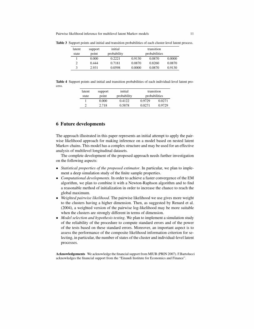
About the distribution of each cluster and individual-level latent process, the es-timates of the initial and transition probabilities are reported in Table 3 and 4. Forboth processes, we observe that the states are well separated and the second state isthe one with the highest initial probability. Moreover, the estimates of the transitionmatrices show that the cluster-level latent process has a lower persistence than theindividual-level latent process.

Finally, we tried to simplify the model selected above by restricting the transitionmatrix of each latent process to be diagonal, so that transition between latent statesis not allowed. In particular, the model in which the transition matrix at cluster-levelis diagonal has a slightly larger value of CLIC equal to -29,706. On the other hand,the restriction that the transition matrix at individual-level is diagonal leads to astrong decrease of CLIC, which is equal to -29,757. We then retain the model inwhich latent transition is allowed both at cluster and at individual level.


Table 3 Support points and initial and transition probabilities of each cluster-level latent process.

latent support initial transitionstate point probability probabilities

1 0.000 0.2221 0.9130 0.0870 0.00002 0.444 0.7181 0.0870 0.8260 0.08703 2.931 0.0598 0.0000 0.0870 0.9130

Table 4 Support points and initial and transition probabilities of each individual-level latent pro-cess.

latent support initial transitionstate point probability probabilities

1 0.000 0.4122 0.9729 0.02712 2.718 0.5878 0.0271 0.9729

6 Future developments

The approach illustrated in this paper represents an initial attempt to apply the pair-wise likelihood approach for making inference on a model based on nested latentMarkov chains. This model has a complex structure and may be used for an effectiveanalysis of multilevel longitudinal datasets.

The complete development of the proposed approach needs further investigationon the following aspects:

• Statistical properties of the proposed estimator. In particular, we plan to imple-ment a deep simulation study of the finite sample properties.

• Computational developments. In order to achieve a faster convergence of the EMalgorithm, we plan to combine it with a Newton-Raphson algorithm and to finda reasonable method of initialization in order to increase the chance to reach theglobal maximum.

• Weighted pairwise likelihood. The pairwise likelihood we use gives more weightto the clusters having a higher dimension. Then, as suggested by Renard et al.(2004), a weighted version of the pairwise log-likelihood may be more suitablewhen the clusters are strongly different in terms of dimension.

• Model selection and hypothesis testing. We plan to implement a simulation studyof the reliability of the procedure to compute standard errors and of the powerof the tests based on these standard errors. Moreover, an important aspect is toassess the performance of the composite likelihood information criterion for se-lecting, in particular, the number of states of the cluster and individual-level latentprocesses.

Acknowledgements We acknowledge the financial support from MIUR (PRIN 2007). F.Bartolucciacknowledges the financial support from the “Einaudi Institute for Economics and Finance”.


References

Altman, R.M. (2007). Mixed hidden Markov models: an extension of the hidden Markov model tothe longitudinal data setting. Journal of the American Statistical Association 102, 201–210.

Asparouhov, T., Muthen, B. (2008). Multilevel mixture models. In: G.R. Hancock, K.M. Samuel-son (Eds.), Advances in latent variable mixture model, Information Age Publishing, Charlotte,NC.

Bartolucci, F. (2006). Likelihood inference for a class of latent Markov models under linear hy-potheses on the transition probabilities. Journal of the Royal Statistical Society, series B 68,155–178.

Bartolucci, F., Lupparelli, M. (2007). The multilevel latent Markov model. In: J. del Castillo, A.Espinal, P. Puig (Eds.), Proceedings of the 22nd International Workshop on Statistical Mod-elling.

Bartolucci, F., Nigro, V. (2007). Maximum likelihood estimation of an extended latent Markovmodel for clustered binary panel data. Computational Statistics and Data Analysis 51, 3470–3483.

Bartolucci, F., Pennoni, F., Lupparelli, M. (2008). Likelihood inference for the latent Markov Raschmodel. In: C. Huber, N. Limnios, M. Mesbah, N. Nikulin (Eds.), Mathematical Methods forSurvival Analysis, Reliability and Quality of Life, Wiley.

Bartolucci, F., Lupparelli, M., Montanari, G.E. (2009). Latent Markov model for binary longitu-dinal data: an application to the performance evaluation of nursing homes. Annals of AppliedStatistics 3, 611–636.

Bartolucci, F., Farcomeni, A., Pennoni, F. (2010a). An overview of latent Markov models for lon-gitudinal categorical data. Technical report, http://arxivorg/abs/10032804.

Bartolucci, F., Pennoni, F., Vittadini, G. (2010b). Assessment of school performance through amultilevel latent Markov Rasch model. Technical report, arXiv:0909.4961v1.

Baum, L., Petrie, T., Soules, G., Weiss, N. (1970). A maximization technique occurring in the sta-tistical analysis of probabilistic functions of Markov chains. Annals of Mathematical Statistics41, 164–171.

Cox, D.R., Reid, N. (2004). A note on pseudolikelihood constructed from marginal densities.Biometrika 91, 729–737.

Dempster, A.P., Laird, N.M., Rubin, D.B. (1977). Maximum likelihood from incomplete data viathe EM algorithm (with discussion). Journal of the Royal Statistical Society, Series B 39, 1–38.

Hjort, N.L., Varin, C. (2008). ML, PL, QL in Markov chain models. Scandinavian Journal ofStatistics 35, 64–82.

Langeheine, R., van de Pol, F. (1990). A unifying framework for markov modeling in discretespace and discrete time. Sociological Methods and Research 18, 416–441.

Levinson, S.E., Rabiner, L.R., Sondhi, M.M. (1983). An introduction to the application of thetheory of probabilistic functions of a Markov process to automatic speech recognition. BellSystem Technical Journal 62, 1035–1074.

Lindsay, B. (1988). Composite likelihood methods. In: N. Prabhu (Ed.), Statistical Inference fromStochastic Process, American Mathematical Society, Providence.

MacDonald, I.L., Zucchini, W. (1997). Hidden Markov and other Models for Discrete-Valued TimeSeries. Chapman and Hall, London.

Renard, D., Molenberghs, G., Geys, H. (2004). A pairwise likelihood approach to estimation inmultilevel probit models. Computational Statistics and Data Analysis 44, 649–667.

Varin, C., Czado, C. (2010). A mixed autoregressive probit model for ordinal longitudinal data.Biostatistics 11, 127–138.

Varin, C., Vidoni, P. (2005). A note on the composite likelihood inference and model selection.Biometrika 92, 519–528.

Wiggins, L. (1973). Panel Analysis: Latent probability models for attitude and behavious pro-cesses. Elsevier, Amsterdam.

Pairwise likelihood inference for multilevel latent Markov models

Documents

Transcript of Pairwise likelihood inference for multilevel latent Markov models