Likelihood Analysis of the Minimal AMSB Model - PUBDB

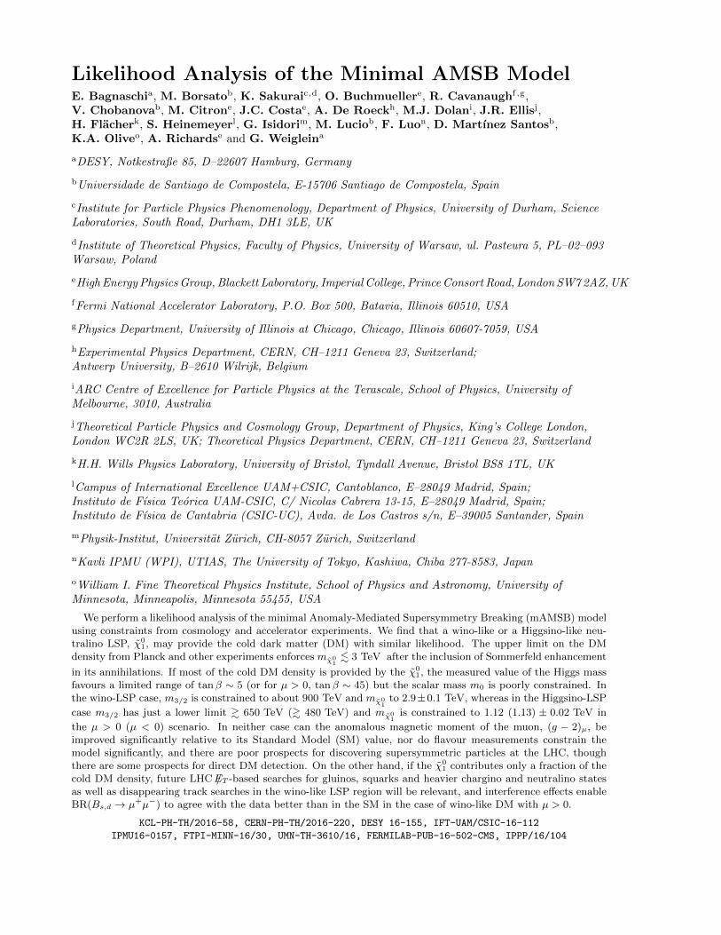
Likelihood Analysis of the Minimal AMSB ModelE. Bagnaschia, M. Borsatob, K. Sakuraic,d, O. Buchmuellere, R. Cavanaughf ,g,V. Chobanovab, M. Citrone, J.C. Costae, A. De Roeckh, M.J. Dolani, J.R. Ellisj,H. Flacherk, S. Heinemeyerl, G. Isidorim, M. Luciob, F. Luon, D. Martınez Santosb,K.A. Oliveo, A. Richardse and G. Weigleina

aDESY, Notkestraße 85, D–22607 Hamburg, Germany

bUniversidade de Santiago de Compostela, E-15706 Santiago de Compostela, Spain

cInstitute for Particle Physics Phenomenology, Department of Physics, University of Durham, ScienceLaboratories, South Road, Durham, DH1 3LE, UK

dInstitute of Theoretical Physics, Faculty of Physics, University of Warsaw, ul. Pasteura 5, PL–02–093Warsaw, Poland

eHigh Energy Physics Group, Blackett Laboratory, Imperial College, Prince Consort Road, London SW7 2AZ, UK

fFermi National Accelerator Laboratory, P.O. Box 500, Batavia, Illinois 60510, USA

gPhysics Department, University of Illinois at Chicago, Chicago, Illinois 60607-7059, USA

hExperimental Physics Department, CERN, CH–1211 Geneva 23, Switzerland;Antwerp University, B–2610 Wilrijk, Belgium

iARC Centre of Excellence for Particle Physics at the Terascale, School of Physics, University ofMelbourne, 3010, Australia

jTheoretical Particle Physics and Cosmology Group, Department of Physics, King’s College London,London WC2R 2LS, UK; Theoretical Physics Department, CERN, CH–1211 Geneva 23, Switzerland

kH.H. Wills Physics Laboratory, University of Bristol, Tyndall Avenue, Bristol BS8 1TL, UK

lCampus of International Excellence UAM+CSIC, Cantoblanco, E–28049 Madrid, Spain;Instituto de Fısica Teorica UAM-CSIC, C/ Nicolas Cabrera 13-15, E–28049 Madrid, Spain;Instituto de Fısica de Cantabria (CSIC-UC), Avda. de Los Castros s/n, E–39005 Santander, Spain

mPhysik-Institut, Universitat Zurich, CH-8057 Zurich, Switzerland

nKavli IPMU (WPI), UTIAS, The University of Tokyo, Kashiwa, Chiba 277-8583, Japan

oWilliam I. Fine Theoretical Physics Institute, School of Physics and Astronomy, University ofMinnesota, Minneapolis, Minnesota 55455, USA

We perform a likelihood analysis of the minimal Anomaly-Mediated Supersymmetry Breaking (mAMSB) modelusing constraints from cosmology and accelerator experiments. We find that a wino-like or a Higgsino-like neu-tralino LSP, χ0

1, may provide the cold dark matter (DM) with similar likelihood. The upper limit on the DMdensity from Planck and other experiments enforces mχ0

1. 3 TeV after the inclusion of Sommerfeld enhancement

in its annihilations. If most of the cold DM density is provided by the χ01, the measured value of the Higgs mass

favours a limited range of tanβ ∼ 5 (or for µ > 0, tanβ ∼ 45) but the scalar mass m0 is poorly constrained. Inthe wino-LSP case, m3/2 is constrained to about 900 TeV and mχ0

1to 2.9±0.1 TeV, whereas in the Higgsino-LSP

case m3/2 has just a lower limit & 650 TeV (& 480 TeV) and mχ01

is constrained to 1.12 (1.13) ± 0.02 TeV in

the µ > 0 (µ < 0) scenario. In neither case can the anomalous magnetic moment of the muon, (g − 2)µ, beimproved significantly relative to its Standard Model (SM) value, nor do flavour measurements constrain themodel significantly, and there are poor prospects for discovering supersymmetric particles at the LHC, thoughthere are some prospects for direct DM detection. On the other hand, if the χ0

1 contributes only a fraction of thecold DM density, future LHC /ET -based searches for gluinos, squarks and heavier chargino and neutralino statesas well as disappearing track searches in the wino-like LSP region will be relevant, and interference effects enableBR(Bs,d → µ+µ−) to agree with the data better than in the SM in the case of wino-like DM with µ > 0.

KCL-PH-TH/2016-58, CERN-PH-TH/2016-220, DESY 16-155, IFT-UAM/CSIC-16-112

IPMU16-0157, FTPI-MINN-16/30, UMN-TH-3610/16, FERMILAB-PUB-16-502-CMS, IPPP/16/104

2

1. Introduction

In previous papers [1–7] we have presented like-lihood analyses of the parameter spaces of vari-ous scenarios for supersymmetry (SUSY) break-ing, including the CMSSM [8], in which softSUSY breaking parameters are constrained to beuniversal at the grand unification scale, mod-els in which Higgs masses are allowed to benon-universal (NUHM1,2) [9, 10], a model inwhich 10 soft SUSY-breaking parameters weretreated as free phenomenological parameters (thepMSSM10) [11] and one with SU(5) GUT bound-ary conditions on soft supersymmetry-breakingparameters [12]. These analyses took into ac-count the strengthening direct constraints fromsparticle searches at the LHC, as well as indirectconstraints based on electroweak precision ob-servables (EWPOs), flavour observables and thecontribution to the density of cold dark matter(CDM) in the Universe from the lightest super-symmetric particle (LSP), assuming that it is aneutralino and that R-parity is conserved [13].In particular, we analysed the prospects withinthese scenarios for discovering SUSY at the LHCand/or in future direct dark matter searches [5].

In this paper we extend our previous analysesof GUT-based models [1–6] by presenting a likeli-hood analysis of the parameter space of the mini-mal scenario for anomaly-mediated SUSY break-ing (the mAMSB) [14, 15]. The spectrum ofthis model is quite different from those of theCMSSM, NUHM1 and NUHM2, with a differ-ent composition of the LSP. Consequently, dif-ferent issues arise in the application of the ex-perimental constraints, as we discuss below. Inthe mAMSB there are 3 relevant continuous pa-rameters, the gravitino mass, m3/2, which setsthe scale of SUSY breaking, the supposedly uni-versal soft SUSY-breaking scalar mass1, m0, andthe ratio of Higgs vacuum expectation values,tanβ, to which may be added the sign of theHiggsino mixing parameter, µ. The LSP is ei-ther a Higgsino-like or a wino-like neutralino χ0

1.

1In pure gravity-mediated models [16], m0 is constrainedto be equal to the gravitino mass, resulting in a two-parameter model in which tanβ is strongly constrainedto a value near 2.

In both cases the χ01 is almost degenerate with

its chargino partner, χ±1 . It is well known that,

within this mAMSB framework, if one requiresthat a wino-like χ0

1 is the dominant source ofthe CDM density indicated by Planck measure-ments of the cosmic microwave background radi-ation, namely ΩCDMh

2 = 0.1186 ± 0.0020 [17],mχ0

1' 3 TeV [18, 19] after inclusion of Sommer-

feld enhancement effects [20]. If instead the CDMdensity is to be explained by a Higgsino-like χ0

1,mχ0

1takes a value of 1.1 TeV. In both cases, spar-

ticles are probably too heavy to be discoveredat the LHC, and supersymmetric contributionsto EWPOs, flavour observables and (g − 2)µ aresmall.

In the first part of our likelihood analysis ofthe mAMSB parameter space, we combine theassumption that the LSP is the dominant sourceof CDM with other measurements, notably ofthe mass of the Higgs boson, Mh = 125.09 ±0.24 GeV [21] (including the relevant theory un-certainties [22]) and its production and decayrates [23]. In addition to solutions in which theχ0

1 is wino- or Higgsino-like, we also find less-favoured solutions in which the χ0

1 is a mixedwino-Higgsino state. In the wino case, whereasm3/2 and hence mχ0

1are relatively well deter-

mined, as is the value of tanβ, the value of m0 isquite poorly determined, and there is little differ-ence between the values of the global likelihoodfunctions for the two signs of µ. On the otherhand, in the case of a Higgsino-like χ0

1, while tanβhas values around 5, m0 and m3/2 are only con-strained to be larger than 20 TeV and 600 TeV,respectively, in the positive µ case. For negativeµ, the m0 and m3/2 constraints are lowered to18 TeV and 500 TeV, respectively.

If there is some other contribution to the CDM,so that Ωχ0

1< ΩCDM, the SUSY-breaking mass

scale m3/2 can be reduced, and hence also mχ01,

although the value of Mh still imposes a signifi-cant lower limit. In this case, some direct searchesfor sparticles at the LHC also become relevant,notably /ET -based searches for gluinos, squarksand heavier chargino and neutralino states as wellas disappearing track searches for the next-to-LSP charged wino. We discuss the prospects forsparticle searches at the LHC in this case and

3

at the 100 TeV FCC-hh collider, and also findthat some deviations from Standard Model (SM)predictions for flavour observables may becomeimportant, notably BR(b → sγ) and BR(Bs,d →µ+µ−).

Using the minimum value of the χ2 likeli-hood function and the number of effective de-grees of freedom (excluding the constraint fromHiggsSignals, as was done in [2–4]) leads to anestimate of ∼ 11% for the χ2 probability of themAMSB model if most of the CDM is due to theχ0

1, for both signs of µ in both the wino- andHiggsino-like cases. When this CDM condition isrelaxed, the χ2 probability is unchanged if µ < 0,but increases to 18% in the wino-like LSP caseif µ > 0 thanks to improved consistency with theexperimental measurement of BR(Bs,d → µ+µ−).These χ2 probabilities for the mAMSB modelcannot be compared directly with those foundpreviously for the CMSSM [2], the NUHM1 [2],the NUHM2 [3] and the pMSSM10 [4], since thosemodels were studied with a different dataset thatincluded an older set of LHC data.

The outline of this paper is as follows. In Sec-tion 2 we review briefly the specification of themAMSB model. In Section 3 we review our im-plementations of the relevant theoretical, phe-nomenological, experimental, astrophysical andcosmological constraints, including those from theflavour and Higgs sectors, and from LHC anddark matter searches (see [4, 6] for details of ourother LHC search implementations). In the caseof dark matter we describe in detail our imple-mentation of Sommerfeld enhancement in the cal-culation of the relic CDM density. Section 4 re-views the MasterCode framework. Section 5 thenpresents our results, first under the assumptionthat the lightest neutralino χ0

1 is the dominantform of CDM, and then in the more general casewhen other forms of CDM may dominate. ThisSection is concluded by the presentation and dis-cussion of the χ2 likelihood functions for observ-ables of interest. Finally, we present our conclu-sions in Section 6.

2. Specification of the mAMSB Model

In AMSB, SUSY breaking arises via a loop-induced super-Weyl anomaly [14]. Since thegaugino masses M1,2,3 are suppressed by loopfactors relative to the gravitino mass, m3/2, thelatter is fairly heavy in this scenario (m3/2 &20 TeV) and the wino-like states are lighter thanthe bino-like ones, with the following ratios ofgaugino masses at NLO: |M1| : |M2| : |M3| ≈ 2.8 :1 : 7.1. Pure AMSB is, however, an unrealisticmodel, because renormalization leads to negativesquared masses for sleptons and, in order to avoidtachyonic sleptons, the minimal AMSB scenario(mAMSB) adds a constant m2

0 to all squaredscalar masses [15]. Thus the mAMSB modelhas three continuous free parameters: m3/2, m0

and the ratio of Higgs vevs, tanβ. In addition,the sign of the Higgsino mixing parameter, µ,is also free. The trilinear soft SUSY-breakingmass terms, Ai, are determined by anomalies, likethe gaugino masses, and are thus proportional tom3/2. The µ term and the Higgs bilinear, B, aredetermined phenomenologically via the minimiza-tion of the Higgs potential, as in the CMSSM.

The following are some characteristic featuresof mAMSB: near mass-degeneracy of the left andright sleptons: mlR

≈ mlL, and of the light-

est chargino and neutralino, mχ±1≈ mχ0

1. The

mass hierarchy between sleptons and gauginos isdependent on the numerical values of the inputparameters, and the squark masses are typicallyvery heavy, because they contain a term propor-tional to g4

3m23/2. In addition, the measured Higgs

mass and the relatively low values of the trilinearsAi together imply that the stop masses must alsobe relatively high. The LSP composition may bewino-, Higgsino-like or mixed, as we discuss inmore detail below.

3. Implementations of Constraints

Our treatments in this paper of many of therelevant constraints follow very closely the imple-mentations in our previous analyses which wererecently summarized in [6]. In the followingsubsections we review the implementations, high-lighting new constraints and instances where we

4

implement constraints differently from our previ-ous work.

3.1. Flavour, Electroweak and Higgs Con-straints

Constraints from B-physics and K-physics ob-servables are the same as in [6]2. In particular,we include the recent ATLAS result in our globalcombination of measurements of BR(Bs,d →µ+µ−) [25]. In contrast to our previous stud-ies [2–6], in this study we do not evaluate in-dependently the constraints from EWPOs, sincefor SUSY-breaking parameters in the multi-TeVrange they are indistinguishable from the Stan-dard Model values within the current experi-mental uncertainties, as we have checked usingFeynWZ [26]. The only exception is the massof the W boson, MW , which is evaluated us-ing FeynHiggs3. For the other EWPOs we usethe theoretical and experimental values given inthe review [27]. We use the combination of AT-LAS and CMS measurements of the mass of theHiggs boson: Mh = 125.09 ± 0.24 GeV [21].We use a beta-version of the FeynHiggs 2.12.1

code [22, 28] to evaluate the constraint this im-poses on the mAMSB parameter space. It im-proves on the FeynHiggs versions used for pre-vious analyses [2–5] by including two-loop QCDcorrections in the evaluation of the DR run-ning top mass and an improved evaluation ofthe top mass in the DR-on-shell conversion forthe scalar tops. At low values of mt1

, we use,as previously, a one-σ theoretical uncertainty of1.5 GeV. In view of the larger theoretical un-certainty at large input parameter values, thisuncertainty is smoothly inflated up to 3.0 GeVat mt1

> 7.5 TeV, as a conservative estimate.The χ2 contributions of 85 Higgs search chan-nels from LHC and Tevatron are evaluated usingHiggsSignals [23] and HiggsBounds [29, 30] asdetailed in our previous paper [6].

2For a previous study of the impact of flavour constraintson the mAMSB model, see [24].3We imposed SU(2) symmetry on the soft SUSY-breakingterms in the DR-on-shell conversion of the parameters inthe scalar top/bottom sector, leading to a small shift inthe values of the scalar bottom masses.

3.2. LHC ConstraintsIf the entire CDM relic density is provided by

the lightest neutralino, all sparticles are heavy,and the current results of the direct sparticlesearches at the LHC have no impact on ourglobal fit, though there is some impact from H/Asearches [31, 32]. On the other hand, if χ0

1 ac-counts only for a fraction of the relic CDM den-sity, some sparticles can be light enough to beproduced at the LHC. However, as we discuss inmore detail later, even for this case we find thatthe sleptons, the first two generations of squarksand the third-generation squarks are heavier than0.7, 3.5 and 2.5 TeV at the 2σ level, respectively,well beyond the current LHC sensitivities [33–35].On the other hand, gluinos and winos can be aslight as 2.5 and 0.5 TeV, respectively, at the 2σlevel, so we have considered in more detail theconstraints from searches at the LHC. Currentlythey do not impact the 68 and 95% CL rangeswe find for the mAMSB, but some impact can beexpected for future LHC runs, as we discuss inSection 5.4.

3.3. Dark Matter Constraints3.3.1. Density Calculations Implementing

Sommerfeld EnhancementFor a wino-like dark matter particle, the non-

perturbative Sommerfeld effect [20] needs to betaken into account in the calculation of the ther-mal relic abundance. Dedicated studies have beenperformed in the literature [18, 19], with the re-sult that the correct relic abundance is obtainedfor mχ0

1' 3.1 TeV after inclusion of Sommerfeld

enhancement in the thermally-averaged coannihi-lation cross sections, compared to mχ0

1' 2.3 TeV

at tree level.Because of the large number of points in our

mAMSB sample, we seek a computationally-efficient implementation of the Sommerfeld en-hancement. We discuss this now, and considerits implications in the following subsections.

It is sufficient for our χ2 likelihood analysisto use a phenomenological fit for the Sommer-feld enhancement that is applicable near 3.1 TeV.One reason is that, away from ∼ 3.1 TeV, theχ2 price rises rapidly due to the very small un-certainty in the Planck result for ΩCDMh

2. An-

5

other reason is that the enhancement factor de-pends very little on the particle spectrum andmostly on mχ0

1. Therefore, we extract the Som-

merfeld factor by using a function to fit the ‘non-perturbative’ curve in the right panel of Fig. 2in [18]. One can see that the curve has a dipat ∼ 2.4 TeV, due to the appearance of a loosely-bound state. The calculated relic abundance nearthe dip is much smaller than the Planck value,so it gives a very large χ2, and therefore we donot bother to fit the dip. Considering that theYukawa potential approaches the Coulomb limitfor mχ0

1 MW , and that only the electromag-

netic force is relevant for mχ01 MW , we fit the

annihilation cross section using 4,

aeff ≡ aeffSE=0

[(cpmSαem + 1− cpm)(

1− exp(−κMW /mχ01))

+Sα2 exp(−κMW /mχ01)], (1)

where aeff is the effective s-wave coannihilationcross section (including the Sommerfeld enhance-ment) for the wino system including the wino-like LSP, χ0

1, and the corresponding chargino,χ±

1 , and aeffSE=0 is the effective s-wave coanni-hilation cross section calculated ignoring the en-hancement. The latter is defined as

aeffSE=0 ≡∑i,j

aijrirj , (2)

where ri ≡ gi (1 + ∆i)3/2

exp(−∆imχ01/T )/geff ,

and geff ≡∑k gk (1 + ∆k)

3/2exp(−∆kmχ0

1/T )

expressed as functions of the temperature, T , atwhich the coannihilations take place. The indicesrefer to χ0

1, χ+1 and χ−

1 , and gi is the numberof degrees of freedom, which is 2 for each of thethree particles, ∆i ≡ (mi/mχ0

1−1), aij is the total

s-wave (co)annihilation cross section for the pro-cesses with incoming particles i and j, and cpm

is the fraction of the contribution of the χ+1 χ

−1

s-wave cross section in aeffSE=0, namely,

cpm ≡2aχ+

1 χ−1

aeffSE=0

rχ+1rχ−

1. (3)

4We emphasize that one can choose a different fitting func-tion, as long as the fit is good near 3.1 TeV.

In practice, since mχ+1−mχ0

1' 0.16 GeV, which

is much smaller than the typical temperatureof interest in the calculation of the relic abun-dance for mχ0

1near 3.1 TeV, we have aeffSE=0 '

(aχ01χ

01+4aχ0

1χ+1

+2aχ+1 χ

−1

+2aχ+1 χ

+1

)/9, and cpm '29aχ+

1 χ−1/aeffSE=0. In Eq. (1), Sαem and Sα2 are

the thermally-averaged s-wave Sommerfeld en-hancement factors for attractive Coulomb poten-tials with couplings αem and α2, respectively. Weuse the function given in Eq. (11) of [36] for thesequantities, namely

Sαx≡ 1 + 7y/4 + 3y2/2 + (3/2− π/3)y3

1 + 3y/4 + (3/4− π/6)y2, (4)

where y ≡ αx√πmχ0

1/T .

Because the curve in [18] is obtained by takingthe massless limit of the SM particles in aij , we dothe same for our fit to obtain the fitting parameterκ. We find that a κ = O(1) can give a good fitfor the curve, and that the fit is not sensitive tothe exact value of κ. We choose κ = 6 in ourcalculation, which gives a good fit around mχ0

1'

3.1 TeV, in particular.Eq. (1) is used in our calculation of the relic

abundance Ωχ01h2 for mAMSB models, for which

we evaluate aeffSE=0 and cpm for any parame-ter point using SSARD [37]. The perturbative p-wave contribution is also included. We note that,whereas the Sommerfeld enhancement dependsalmost entirely on mχ0

1, the values of aeff and

cpm depend on the details of the supersymmetricparticle spectrum. In particular, due to a cancel-lation between s- and t-channel contributions inprocesses with SM fermion anti-fermion pairs inthe final states, aeffSE=0 becomes smaller whenthe sfermion masses are closer to mχ0

1.

For a small subset of our mAMSB parametersample, we have compared results obtained fromour approximate implementation of the Sommer-feld enhancement in the case of wino dark matterwith more precise results obtained with SSARD.As seen in the left panel of Fig. 1, our imple-mentation (red line) yields results for the relicdensity that are very similar to those of completecalculations (black dots). In the right panel weplot the ratio of the relic density calculated usingour simplified Sommerfeld implementation for the

6

sub-sample of mAMSB points to SSARD results,connecting the points at different mχ0

1by a con-

tinuous blue line. We see that our Sommerfeldimplementation agrees with the exact results atthe . 2% level (in particular whenmχ0

1∼ 3 TeV),

an accuracy that is comparable to the current ex-perimental uncertainty from the Planck data. Weconclude that our simplified Sommerfeld imple-mentation is adequate for our general study ofthe mAMSB parameter space 5.

Figure 2 illustrates the significance of the Som-merfeld enhancement via a dedicated scan of the(m0,m3/2) plane for tanβ = 5 using SSARD. Thepink triangular region at large m0 and relativelysmall m3/2 is excluded because there are no con-sistent solutions to the electroweak vacuum con-ditions in that region. The border of that regioncorresponds to the line where µ2 = 0, like thatoften encountered in the CMSSM at low m1/2

and large m0 near the so-called focus-point region[40]. The dark blue strips indicate where the cal-culated χ0

1 density falls within the 3-σ CDM den-sity range preferred by the Planck data [17], andthe red dashed lines are contours of Mh (labelledin GeV) calculated using FeynHiggs 2.11.3 6.The Sommerfeld enhancement is omitted in theleft panel and included in the right panel of Fig. 2.We see that the Sommerfeld enhancement in-creases the values of m3/2 along the prominentnear-horizontal band (where the LSP is predomi-nantly wino) by ∼ 200 TeV, which is much largerthan the uncertainties associated with the CDMdensity range and our approximate implementa-tion of the Sommerfeld enhancement. We stressthat any value of m3/2 below this band would alsobe allowed if the χ0

1 provides only a fraction of thetotal CDM density.

3.3.2. Higgsino RegionWe note also the presence in both panels of

a very narrow V-shaped diagonal strip runningclose to the electroweak vacuum boundary, wherethe χ0

1 LSP has a large Higgsino component as

5As stated above, a full point-by-point calculation of therelic density would be impractical for our large sample ofmAMSB parameters.6This version is different from that used for our χ2 evalua-tion, and is used here for illustration only. The numericaldifferences do not change the picture in a significant way.

mentioned previously. As this Higgsino strip israther difficult to see, we show in Fig. 3 a blowupof the Higgsino region for µ > 0 (the correspond-ing region for µ < 0 is similar), where we havethickened artificially the Higgsino strips by shad-ing dark blue regions with m3/2 ≤ 9.1× 105 GeVwhere 0.1126 ≤ Ωχ0

1h2 ≤ 0.2. As the nearly

horizontal wino strip approaches the electroweaksymmetry breaking boundary, the blue strip de-viates downward to a point, and then tracks theboundary back up to higher m0 and m3/2, form-ing a slanted V shape.

The origin of these two strips can be under-stood as follows. In most of the triangular regionbeneath the relatively thick horizontal strip, theLSP is a wino with mass below 3 TeV, and therelic density is below the value preferred by thePlanck data. For fixed m3/2, as m0 is increased,µ drops so that, eventually, the Higgsino mass be-comes comparable to the wino mass. When µ >1 TeV, the crossover to a Higgsino LSP (whichoccurs when µ . M2) yields a relic density thatreaches and then exceeds the Planck relic den-sity, producing the left arm of the slanted V-shapestrip near the focus-point boundary where coan-nihilations between the wino and Higgsino are im-portant. As one approaches closer to the focuspoint, µ continues to fall and, when µ ' 1 TeV,the LSP becomes mainly a Higgsino and its relicdensity returns to the Planck range, thus produc-ing right arm of the slanted V-shape strip corre-sponding to the focus-point strip in the CMSSM.In the right panel of Fig. 2 and in Fig. 3 the tipof the V where these narrow dark matter stripsmerge occurs when m0 ∼ 1.8× 104 GeV.

In the analysis below, we model the transitionregion by using Micromegas 3.2 [41] to calcu-late the relic density, with a correction in theform of an analytic approximation to the Som-merfeld enhancement given by SSARD that takesinto account the varying wino and Higgsino frac-tions in the composition of the LSP. In this waywe interpolate between the wino approximationbased on SSARD discussed above for winos, andMicromegas 3.2 for Higgsinos.

Comparing the narrowness of the strips in Figs.2 and 3 with the thickness of the near-horizontalwino strip, it is clear that they are relatively finely

7

[TeV]0

1χ ~

m

2.6 2.7 2.8 2.9 3 3.1 3.2 3.3 3.4

2h

10χ ~

Ω

0.1

0.105

0.11

0.115

0.12

0.125

0.13

0.135

0.14

[TeV]0

1χ ~

m

2.6 2.8 3 3.2 3.4S

SA

RD

)2

h10

χ ~Ω

/(M

C)

2h

10χ ~

Ω(0.8

0.85

0.9

0.95

1

1.05

1.1

1.15

1.2

Figure 1. Calculations of Ωχ01h2 comparing results from SSARD [37] and our simplified treatment of the

Sommerfeld enhancement in the case of wino dark matter. The left panel compares the SSARD calculations(black dots) with our Sommerfeld implementation (red line), and the right panel shows the ratio of thecalculated relic densities, connecting the points in the left panel by a continuous blue line.

0.0 1.0×104 2.0×104 3.0×1043.0×104

1.0×106

124

124 125

125125125

125125125

125

125

126

126

126

126

126

126

126

126

127

127

127

127

127

128

128

128 128

129

129129

129

129

130

130130

130

1.0×104 2.0×104 3.0×1043.0×104

1.0×106

m 3/2 (

GeV)

m0 (GeV)

5.0×105

125

122

123124

126

127

tan β = 5, µ > 0

0.0 1.0×104 2.0×104 3.0×1043.0×104

1.0×106

124

124 125

125125125

125125125

125

125

126

126

126

126

126

126

126

126

127

127

127

127

127

128

128

128 128

129

129129

129

129

130

130130

130

1.0×104 2.0×104 3.0×1043.0×104

1.0×106

m 3/2 (

GeV)

m0 (GeV)

5.0×105

125

122

123124

126

127

tan β = 5, µ > 0

Figure 2. The (m0,m3/2) plane for tanβ = 5 without (left panel) and with (right panel) the Sommerfeldenhancement, as calculated using SSARD [37]. There are no consistent solutions of the electroweak vacuumconditions in the pink shaded triangular regions at lower right. The χ0

1 LSP density falls within the rangeof the CDM density indicated by Planck and other experiments in the dark blue shaded bands. Contoursof Mh calculated using FeynHiggs 2.11.3 (see text) are shown as red dashed lines.

8

1.5×104 2.0×104 3.0×1044.0×105

5.0×105

6.0×105

7.0×105

8.0×105

9.0×105

1.0×106

124

124

125

125125

126

126

126

126

126

126

126

127

127

127

127

127 127

127

127

127

127

127

127

127

128

128

128

128

128128

128

128

128

128

129

129129

129

129

129

129

129

129129

130

130 130

130

130

130

130

130

131

1.5×104 2.0×104 3.0×1044.0×105

5.0×105

6.0×105

7.0×105

8.0×105

9.0×105

1.0×106

m 3/2 (

GeV)

m0 (GeV)

tan β = 5, µ > 0

125

126

127

Figure 3. Blowup of the right panel in Fig. 2. When m3/2 ≤ 9.1× 105 GeV, we shade dark blue regionswith 0.1126 ≤ Ωχ0

1h2 ≤ 0.2 so as to thicken the slanted V-shaped Higgsino LSP strip. Towards the upper

part of the Higgsino strip, there is a thin brown shaded strip that is excluded because the LSP is a chargino.Contours of Mh calculated (labelled in GeV) using FeynHiggs 2.11.3 (see text) are shown as red dashedlines.

tuned. We also note in Fig. 3 a thin brown shadedregion towards the upper part of the V-shapedHiggsino strip that is excluded because the LSPis a chargino.

We also display in these (m0,m3/2) planes con-tours of Mh (labelled in GeV) as calculated usingFeynHiggs 2.11.3 (see above). Bearing in mindthe estimated uncertainty in the theoretical cal-culation of Mh [22], all the broad near-horizontalband and the narrow diagonal strips are compat-ible with the measured value of Mh, both withand without the inclusion of the Sommerfeld en-hancement.

3.3.3. Dark Matter DetectionWe implement direct constraints on the spin-

independent dark matter proton scattering cross

section, σSIp , using the SSARD code [37], as re-

viewed previously [2–6]. As discussed there and inSection 5.5, σSI

p inherits considerable uncertaintyfrom the poorly-constrained 〈p|ss|p〉 matrix ele-ment and other hadronic uncertainties, which arelarger than those associated with the uncertaintyin the local CDM halo density.

We note also that the relatively large annihila-tion cross section of wino dark matter is in tensionwith gamma-ray observations of the Galactic cen-ter, dwarf spheroidals and satellites of the MilkyWay made by the Fermi-LAT and H.E.S.S. tele-scopes [38]. However, there are still considerableambiguities in the dark matter profiles near theGalactic center and in these other objects. In-cluding these indirect constraints on dark matterannihilation in our likelihood analysis would re-

9

quire estimates of these underlying astrophysicaluncertainties [39], which are beyond the scope ofthe present work.

4. Analysis Procedure

4.1. MasterCode FrameworkWe define a global χ2 likelihood function that

combines the theoretical predictions with experi-mental constraints, as done in our previous anal-yses [2–6].

We calculate the observables that go into thelikelihood using the MasterCode framework [1–7], which interfaces various public and privatecodes: SoftSusy 3.7.2 [42] for the spectrum,FeynHiggs 2.12.1 [22, 28] (see Section 3.1)for the Higgs sector, the W boson mass and(g − 2)µ, SuFla [43] for the B-physics observ-ables, Micromegas 3.2 [41] (modified as dis-cussed above) for the dark matter relic den-sity, SSARD [37] for the spin-independent cross-section σSI

p and the wino dark matter relic den-sity, SDECAY 1.3b [44] for calculating sparticlebranching ratios, and HiggsSignals 1.4.0 [23]and HiggsBounds 4.3.1 [29, 30] for calculatingconstraints on the Higgs sector. The codesare linked using the SUSY Les Houches Accord(SLHA) [45].

We use SuperIso [46] and Susy Flavor [47] tocheck our evaluations of flavour observables, andwe have used Matplotlib [48] and PySLHA [49] toplot the results of our analysis.

4.2. Parameter RangesThe ranges of the mAMSB parameters that we

sample are shown in Table 1. We also indicate inthe right column of this Table how we divide theranges of these parameters into segments, as wedid previously for our analyses of the CMSSM,NUHM1, NUHM2, pMSSM10 and SU(5) [2–6].The combinations of these segments constituteboxes, in which we sample the parameter spaceusing the MultiNest package [50]. For each box,we choose a prior for which 80% of the sample hasa flat distribution within the nominal range, and20% of the sample is outside the box in normally-distributed tails in each variable. In this way,our total sample exhibits a smooth overlap be-

tween boxes, eliminating spurious features asso-ciated with box boundaries. Since it is relativelyfine-tuned, we made a dedicated supplementary36-box scan of the Higgsino-LSP region of themAMSB parameter space, requiring the lightestneutralino to be Higgsino-like. We have sampleda total of 11(13)× 106 points for µ > 0 (µ < 0).

5. Results

5.1. Case I: CDM is mainly the lightestneutralino

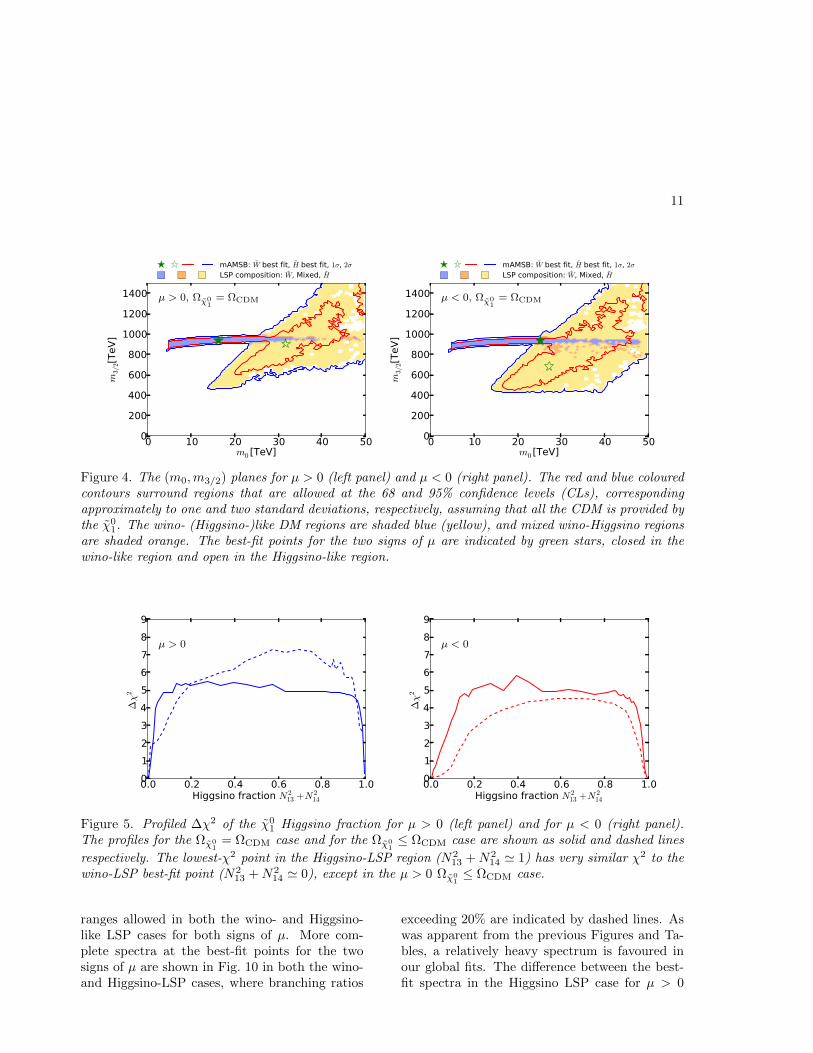
We display in Fig. 4 the (m0,m3/2) planes forour sampling of mAMSB parameters with µ > 0(left panel) and µ < 0 (right panel). The colouredcontours bound regions of parameter space with∆χ2 = 2.30 and ∆χ2 = 5.99 contours, which weuse as proxies for the boundaries of the 68% (red)and 95% (dark blue) CL regions. The best-fitpoints for the two signs of µ are indicated bygreen stars, closed in the case of wino-like DM,open in the case of Higgsino-like DM. The shad-ings in this and subsequent planes indicate thecomposition of the sample point with the low-est χ2 in this projection: in general, there willalso be sample points with a different compositionand (possibly only slightly) larger χ2. Differentshading colours represent the composition of theχ0

1 LSP: a region with Higgsino fraction exceed-ing 90% is shaded yellow, one with wino fractionexceeding 90% is shaded light blue, while othercases are shaded orange 7. Most of blue shad-ing corresponds to a wino-like LSP, and in only asmall fraction of cases to a mixed wino-Higgsinostate. We see that in the case of a wino-like LSP,the regions favoured at the 2-σ level are bandswith 900 TeV . m3/2 . 1000 TeV correspondingto the envelope of the near-horizontal band in theright panel of Fig. 2 and in Fig. 3 that is obtainedwhen profiling over tanβ. For both signs of µ, thelower limit m0 & 5 TeV is due to the τ1 becomingthe LSP.

The yellow Higgsino-LSP regions correspond tothe envelope of the V-shaped diagonal strips seenin Fig. 2 and in Fig. 3. The locations of these di-agonal strips vary significantly with tanβ and mt,

7The uncoloured patches and the irregularities in the con-tours are due to the limitations of our sampling.

10

Parameter Range Generic HiggsinoSegments Segments

m0 ( 0.1 , 50 TeV) 4 6m3/2 ( 10 , 1500 TeV) 3 3tanβ ( 1 , 50) 4 2

Total number of boxes 48 36

Table 1. Ranges of the mAMSB parameters sampled, together with the numbers of segments into whicheach range was divided, and the corresponding number of sample boxes. The numbers of segments andboxes are shown both for the generic scan and for the supplementary scan where we constrain the neutralinoto be Higgsino like.

and their extents are limited at small and largegravitino mass mainly by the Higgs mass con-straint. The best-fit point for the Higgsino-LSPscenario has a total χ2 very similar to the wino-LSP case, as is shown in Fig. 5. The χ2 values atthe best-fit points in the wino- and Higgsino-likeregions for both signs of µ are given in Table 2,together with more details of the fit results (seebelow).

Figs. 6 and 7 display the (tanβ,m0) and(tanβ,m3/2) planes respectively. Both the µ > 0case (left panel) and the µ < 0 case (right panel)are shown, and are qualitatively similar. Thebest-fit points for the two signs of µ are again indi-cated by green stars. Larger m0 and m3/2 valuesare allowed in the Higgsino-LSP case, providedthat tanβ is small. Values of tanβ & 3 are al-lowed at the 95% CL with an upper limit at 48only in the µ > 0 case. There are regions favouredat the 68% CL with small values of tanβ . 10 inboth the wino- and Higgsino-like cases for bothsigns of µ. In addition, for µ > 0 there is an-other 68% CL preferred region in the wino case attanβ & 35, where supersymmetric contributionsimprove the consistency with the measurementsof BR(Bs,d → µ+µ−), as discussed in more detailin Section 5.3 8.

The parameters of the best-fit points for µ > 0and µ < 0 are listed in Table 2, together withtheir 68% CL ranges corresponding to ∆χ2 = 1.We see that at the 68% CL the range of tanβ

8The diagonal gap in the left panel of Fig. 7 for µ > 0is in a region where our numerical calculations encounterinstabilities.

is restricted to low values for both LSP compo-sitions, with the exception of the µ > 0 wino-LSP case, where also larger tanβ values around45 are allowed. In the wino-LSP scenario, m3/2

is restricted to a narrow region around 940 TeVand m0 is required to be larger than 4 TeV. Theprecise location of the Higgsino-LSP region de-pends on the spectrum calculator employed, andalso on the version used. These variations canbe as large as tens of TeV for m0 or a couple ofunits for tanβ, and can change the χ2 penaltycoming from the Higgs mass. In our implementa-tions, we find that m3/2 can take masses as low as650 TeV (480 TeV) while m0 is required to be atleast 23 TeV (18 TeV) at the 68% CL in the µ > 0(µ < 0) case. This variability is related to the un-certainty in the exact location of the electroweaksymmetry-breaking boundary, which is very sen-sitive to numerous corrections, in particular thoserelated to the top quark Yukawa coupling.

The minimum values of the global χ2 functionfor the two signs of µ are also shown in Table 2, asare the χ2 probability values obtained by combin-ing these with the numbers of effective degrees offreedom. We see that all the cases studied (wino-and Higgsino-like LSP, µ > 0 and µ < 0) havesimilar χ2 probabilities, around 11%.

We show in Fig. 8 the contributions to the to-tal χ2 of the best-fit point in the scenarios withdifferent hypotheses on the sign of µ and the com-position of CDM. In addition, we report the mainχ2 penalties in Table 3.

Figure 9 shows the best fit values (blue lines)of the particle masses and the 68% and 95% CL

11

0 10 20 30 40 50m0 [TeV]

0

200

400

600

800

1000

1200

1400

m3/2

[TeV

]

mAMSB: W best fit, H best fit, 1σ, 2σLSP composition: W, Mixed, H

µ > 0, Ωχ01

= ΩCDM

0 10 20 30 40 50m0 [TeV]

0

200

400

600

800

1000

1200

1400

m3/2

[TeV

]


µ < 0, Ωχ01

= ΩCDM

Figure 4. The (m0,m3/2) planes for µ > 0 (left panel) and µ < 0 (right panel). The red and blue colouredcontours surround regions that are allowed at the 68 and 95% confidence levels (CLs), correspondingapproximately to one and two standard deviations, respectively, assuming that all the CDM is provided bythe χ0

1. The wino- (Higgsino-)like DM regions are shaded blue (yellow), and mixed wino-Higgsino regionsare shaded orange. The best-fit points for the two signs of µ are indicated by green stars, closed in thewino-like region and open in the Higgsino-like region.

0.0 0.2 0.4 0.6 0.8 1.0Higgsino fraction N 2

13 +N 214

0123456789

∆χ

2

µ > 0

0.0 0.2 0.4 0.6 0.8 1.0Higgsino fraction N 2

13 +N 214

0123456789

∆χ

2

µ < 0

Figure 5. Profiled ∆χ2 of the χ01 Higgsino fraction for µ > 0 (left panel) and for µ < 0 (right panel).

The profiles for the Ωχ01

= ΩCDM case and for the Ωχ01≤ ΩCDM case are shown as solid and dashed lines

respectively. The lowest-χ2 point in the Higgsino-LSP region (N213 +N2

14 ' 1) has very similar χ2 to thewino-LSP best-fit point (N2

13 +N214 ' 0), except in the µ > 0 Ωχ0

1≤ ΩCDM case.

ranges allowed in both the wino- and Higgsino-like LSP cases for both signs of µ. More com-plete spectra at the best-fit points for the twosigns of µ are shown in Fig. 10 in both the wino-and Higgsino-LSP cases, where branching ratios

exceeding 20% are indicated by dashed lines. Aswas apparent from the previous Figures and Ta-bles, a relatively heavy spectrum is favoured inour global fits. The difference between the best-fit spectra in the Higgsino LSP case for µ > 0

12

Wino-LSP Higgsino-LSPParameter µ > 0 µ < 0 µ > 0 µ < 0

m0: best-fit value 16 TeV 25 TeV 32 TeV 27 TeV68% range (4, 40) TeV (4, 43) TeV (23, 50) TeV (18, 50) TeV

m3/2: best-fit value 940 TeV 940 TeV 920 TeV 650 TeV68% range (860, 970) TeV (870, 950) TeV (650, 1500) TeV (480, 1500) TeV

tanβ: best-fit value 5.0 4.0 4.4 4.268% range (3, 8) and (42, 48) (3, 7) (3, 7) (3, 7)

χ2/d.o.f 36.4 / 27 36.4 / 27 36.6 / 27 36.4 / 27χ2 probability 10.7% 10.7% 10.2% 10.7%

Table 2. Fit results for the mAMSB assuming that the LSP makes the dominant contribution to the colddark matter density. The 68% CL ranges correspond to ∆χ2 = 1. We also display the values of the globalχ2 function omitting the contributions from HiggsSignals, and the corresponding χ2 probability values.Each mass range is shown for both the wino- and higgsino-LSP scenarios as well as for both signs of µ.

0 10 20 30 40 50tanβ

0

10

20

30

40

50

m0[T

eV]


µ > 0, Ωχ01

= ΩCDM

0 10 20 30 40 50tanβ

0

10

20

30

40

50

m0[T

eV]


µ < 0, Ωχ01

= ΩCDM

Figure 6. The (tanβ,m0) planes for µ > 0 (left panel) and for µ < 0 (right panel), assuming that the χ01

provides all the CDM density. The colouring convention for the shadings and contours is the same as inFig. 4, and the best-fit points for the two signs of µ are again indicated by green stars.

and < 0 reflects the fact that the likelihood func-tion is quite flat in the preferred region of theparameter space. In the Higgsino-LSP case, thespectra are even heavier than the other one witha wino LSP, apart from the gauginos, which arelighter. Overall, these high mass scales, togetherwith the minimal flavor violation assumption, im-plies that there are, in general, no significant de-partures from the SM predictions in the flavoursector or for (g − 2)µ.

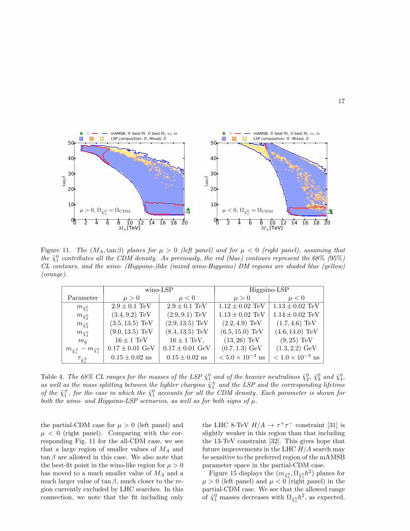
Figure 11 shows the (MA, tanβ) planes for

µ > 0 (left panel) and for µ < 0 (right panel),assuming that the χ0

1 contributes all the CDMdensity. As previously, the red (blue) contoursrepresent the 68% (95%) CL contours, and thewino- (Higgsino-)like DM regions are shaded blue(yellow), and mixed wino-Higgsino regions areshaded orange. We find that the impact of the re-cent LHC 13-TeV constraints on the (MA, tanβ)plane is small in these plots. We see here thatthe large-tanβ 68% CL region mentioned abovecorresponds to MA . 6 TeV.

13

0 10 20 30 40 50tanβ

0

200

400

600

800

1000

1200

1400

m3/2

[TeV

]


µ > 0, Ωχ01

= ΩCDM

0 10 20 30 40 50tanβ

0

200

400

600

800

1000

1200

1400

m3/2

[TeV

]


µ < 0, Ωχ01

= ΩCDM

Figure 7. The (tanβ,m3/2) planes for µ > 0 (left panel) and µ < 0 (right panel), assuming that the χ01

provides all the CDM density. The shadings and colouring convention for the contours are the same asin Fig. 4, and the best-fit points for the two signs of µ are again indicated by green stars.

Ωχ01

= ΩCDM Ωχ01< ΩCDM

W -LSP H-LSP W -LSP H-LSPConstraint µ > 0 µ < 0 µ > 0 µ < 0 µ > 0 µ < 0 µ > 0 µ < 0

σ0had 2.3 2.3 2.3 2.3 2.3 2.3 2.3 2.3Rl 1.5 1.5 1.5 1.5 1.5 1.5 1.5 1.5AbFB 5.8 5.8 5.8 5.8 5.8 5.8 5.8 5.8AeLR 4.0 4.0 4.0 4.0 4.0 4.0 4.0 4.0MW 1.9 1.9 2.1 1.9 1.8 1.8 1.8 1.9

(g − 2)µ 11.2 11.2 11.2 11.2 10.4 11.2 11.2 11.2BR(Bs → µ+µ−) 1.9 1.9 1.9 1.9 0.0 1.9 1.9 1.9

∆MBs/SM∆MBd

1.8 1.8 1.8 1.8 1.6 1.8 1.8 1.8

εK 2.0 2.0 2.0 2.0 2.0 2.0 2.0 2.0∆χ2

HiggsSignals 67.9 67.9 67.9 68.0 68.0 67.9 67.9 68.0

Table 3. The most important contributions to the total χ2 of the best fit points for mAMSB assumingdifferent hypotheses on the composition of the dark matter relic density and on the sign of µ. In theµ > 0 scenario with Ωχ0

1< ΩCDM and W -LSP, the experimental constraints from (g − 2)µand BR(Bs →

µ+µ−) can be accommodated and get a lower χ2 penalty.

As anticipated in Section 1, the wino-LSPis almost degenerate with the lightest chargino,which acquires a mass about 170 MeV largerthrough radiative corrections. Therefore, becauseof phase-space suppression the chargino acquiresa lifetime around 0.15 ns, and therefore may de-cay inside the ATLAS tracker. However, the AT-LAS search for disappearing tracks [51] is insen-

sitive to the large mass ∼ 2.9 TeV expected forthe mAMSB chargino if the LSP makes up all thedark matter. In Section 5.2 we estimate the LHCsensitivity to the lower chargino masses that arepossible if the χ0

1 contributes only a fraction ofthe cold dark matter density. In the Higgsino-LSP case, the chargino has a mass ∼ 1.1 TeV inthe all-DM case, but its lifetime is very short, of

14

0 2 4 6 8 10 12

mt

∆α(5)had(MZ)

MZ

ΓZ

σ0had

Rl

A lFB

Al(Pτ)

Rb

Rc

A bFB

A cFB

Ab

Ac

A eLR

sin2θeff

MW

aEXPµ − aSMµ

Mh

BREXP/SMB→Xsγ

BREXP/SMBs, d→µ + µ −

BREXP/SMB→τν

BREXP/SMB→Xsll

BREXP/SMK→lν

BREXP/SMK→πνν

∆MEXP/SMBs

∆MBs/SM

∆MBd

εK

LHCJets +MET8TeV

LHCJets +MET13TeV

LHCHLCP13TeV

H/A→τ+τ−

ΩCDMh2

σSIp

∆χ2HiggsSignals

µ> 0, Ωχ01= ΩCDM

µ< 0, Ωχ01= ΩCDM

µ> 0, Ωχ01<ΩCDM

µ< 0, Ωχ01<ΩCDM

62 66

∆χ2

Figure 8. All the contributions to the total χ2 forthe best-fit points for mAMSB assuming differenthypotheses on the composition of the dark matterrelic density and on the sign of µ as indicated inthe legend.

the order of few ps.The 68% CL ranges of the neutralino masses,

the gluino mass, the χ±1 − χ0

1 mass splitting and

the χ±1 lifetime are reported in Table 4, assuming

that the χ01 accounts for all the CDM density.

Each parameter is shown for both the wino- andHiggsino-like LSP scenarios and for the two signsof µ.

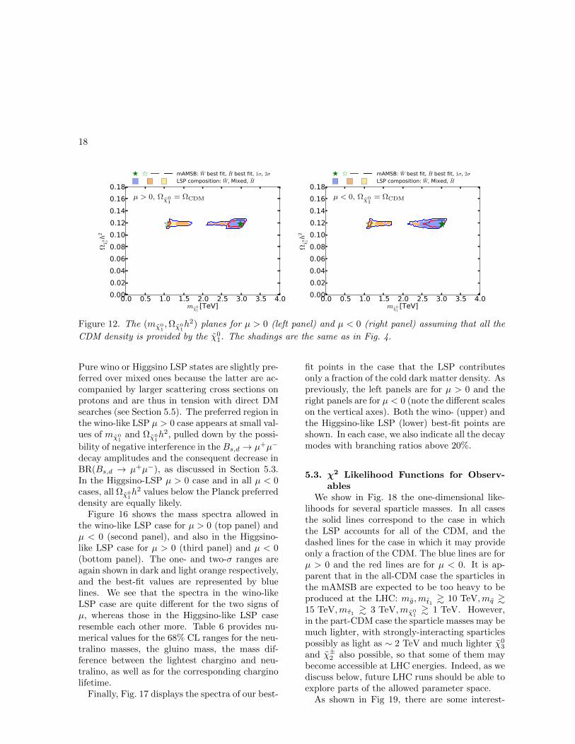
Figure 12 shows our results in the (mχ01,Ωχ0

1h2)

plane in the case when the χ01 is required to pro-

vide all the CDM density, within the uncertaintiesfrom the Planck and other measurements. Theleft panel is for µ > 0 and the right panel is forµ < 0: they are quite similar, with each featuringtwo distinct strips. The strip where mχ0

1∼ 1 TeV

corresponds to a Higgsino LSP near the focus-point region, and the strip where mχ0

1∼ 3 TeV is

in the wino LSP region of the parameter space.In between these strips, the make-up of the LSPchanges as the wino- and Higgsino-like neutralinostates mix, and coannihilations between the threelightest neutralinos and both charginos becomeimportant. The Sommerfeld enhancement variesrapidly (we recall that it is not important in theHiggsino LSP region), causing the relic densityto rise rapidly as well. We expect the gap seenin Fig. 12 to be populated by points with veryspecific values of m0.

5.2. Case II: the LSP does not provide allthe cold dark matter

If the LSP is not the only component of the colddark matter, mχ0

1may be smaller, m3/2 may also

be lowered substantially, and some sparticles maybe within reach of the LHC. The preferred regionsof the (m0,m3/2) planes for µ > 0 (left panel) andµ < 0 (right panel) in this case are shown in theupper panels of Fig 13 9. We see that the winoregion allowed at the 95% CL extends to smallerm3/2 for both signs of µ, and also to larger m0 atm3/2 & 300 TeV when µ < 0. We also see thatthe 68% CL region extends to much larger m0

and m3/2 when µ < 0, and the best-fit point alsomoves to larger masses than for µ > 0, thoughwith smaller tanβ.

9The sharp boundaries at low m0 in the upper panels ofFig 13 are due to the stau becoming the LSP, and thenarrow separation between the near-horizontal portionsof the 68 and 95% CL contours in the upper right panelof Fig. 13 is due to the sharp upper limit on the CDMdensity.

15

Mh0 MH0 MA0 MH± mχ 01mχ 0

2mχ 0

3mχ 0

4mχ ±

1mχ ±

2meL

meRmµL

mµRmτ1

mτ2mqL

mqRmt1

mt2mb1

mb2mg

0.1

1.0

10.0

Part

icle

Mas

ses

[TeV

]

W -LSP for µ > 0, Ωχ01

= ΩCDM


2mχ 0

3mχ 0

4mχ ±

1mχ ±

2meL

meRmµL

mµRmτ1

mτ2mqL

mqRmt1

mt2mb1

mb2mg

0.1

1.0

10.0

Part

icle

Mas

ses

[TeV

]

W -LSP for µ < 0, Ωχ01

= ΩCDM


2mχ 0

3mχ 0

4mχ ±

1mχ ±

2meL

meRmµL

mµRmτ1

mτ2mqL

mqRmt1

mt2mb1

mb2mg

0.1

1.0

10.0

Part

icle

Mas

ses

[TeV

]

H-LSP for µ > 0, Ωχ01

= ΩCDM


2mχ 0

3mχ 0

4mχ ±

1mχ ±

2meL

meRmµL

mµRmτ1

mτ2mqL

mqRmt1

mt2mb1

mb2mg

0.1

1.0

10.0

Part

icle

Mas

ses

[TeV

]

H-LSP for µ < 0, Ωχ01

= ΩCDM

Figure 9. The ranges of masses obtained for the wino-like LSP case with µ > 0 (top panel) and µ < 0(second panel), and also for the Higgsino-like LSP case for µ > 0 (third panel) and µ < 0 (bottom panel),assuming that the LSP makes the dominant contribution to the cold dark matter density.

16

0

5000

10000

15000

20000

25000

30000

35000

40000

Mas

s/

GeV

h0

A0, H0 H±dL, uL, uR, dR

b1, t2

t1˜R, νL, ˜L τ1, ντ , τ2

g

χ01

χ02

χ±1

χ03, χ0

4 χ±2

b2

W -LSP for µ > 0, Ωχ01

= ΩCDM

0

5000

10000

15000

20000

25000

30000

35000

40000

Mas

s/

GeV

h0

A0, H0 H± dL, uL, uR, dR

b1, t2

t1

˜R, νL, ˜L τ1, ντ , τ2

g

χ01

χ02, χ0

3, χ04

χ±1

χ±2

b2

W -LSP for µ < 0, Ωχ01

= ΩCDM

0

5000

10000

15000

20000

25000

30000

35000

40000

Mas

s/

GeV

h0


b1, t2

t1

˜R, νL, ˜L τ1, ντ , τ2

g

χ01, χ0

2 χ±1

χ03

χ04

χ±2

b2

H-LSP for µ > 0, Ωχ01

= ΩCDM

0

5000

10000

15000

20000

25000

30000

35000

40000

Mas

s/

GeV

h0


b1, t2

t1

νL, ˜L, ˜R τ1, ντ , τ2

g

χ01, χ0

2, χ03 χ±

1 , χ±2

χ04

b2

H-LSP for µ < 0, Ωχ01

= ΩCDM

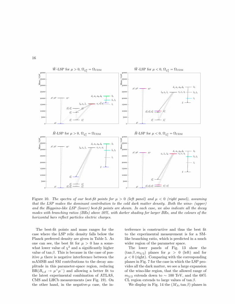
Figure 10. The spectra of our best-fit points for µ > 0 (left panel) and µ < 0 (right panel), assumingthat the LSP makes the dominant contribution to the cold dark matter density. Both the wino- (upper)and the Higgsino-like LSP (lower) best-fit points are shown. In each case, we also indicate all the decaymodes with branching ratios (BRs) above 20%, with darker shading for larger BRs, and the colours of thehorizontal bars reflect particles electric charges.

The best-fit points and mass ranges for thecase where the LSP relic density falls below thePlanck preferred density are given in Table 5. Asone can see, the best fit for µ > 0 has a some-what lower value of χ2 and a significantly highervalue of tanβ. This is because in the case of pos-itive µ there is negative interference between themAMSB and SM contributions to the decay am-plitude in this parameter-space region, reducingBR(Bs,d → µ+µ−) and allowing a better fit tothe latest experimental combination of ATLAS,CMS and LHCb measurements (see Fig. 19). Onthe other hand, in the negative-µ case, the in-

terference is constructive and thus the best fitto the experimental measurement is for a SM-like branching ratio, which is predicted in a muchwider region of the parameter space.

The lower panels of Fig. 13 show the(tanβ,m3/2) planes for µ > 0 (left) and forµ < 0 (right). Comparing with the correspondingplanes in Fig. 7 for the case in which the LSP pro-vides all the dark matter, we see a large expansionof the wino-like region, that the allowed range ofm3/2 extends down to ∼ 100 TeV, and the 68%CL region extends to large values of tanβ.

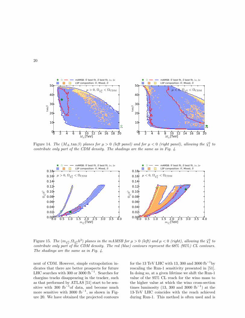
We display in Fig. 14 the (MA, tanβ) planes in

17

0 2 4 6 8 10 12 14 16 18 20MA [TeV]

0

10

20

30

40

50

tanβ


µ > 0, Ωχ01

= ΩCDM

0 2 4 6 8 10 12 14 16 18 20MA [TeV]

0

10

20

30

40

50

tanβ


µ < 0, Ωχ01

= ΩCDM

Figure 11. The (MA, tanβ) planes for µ > 0 (left panel) and for µ < 0 (right panel), assuming thatthe χ0

1 contributes all the CDM density. As previously, the red (blue) contours represent the 68% (95%)CL contours, and the wino- (Higgsino-)like (mixed wino-Higgsino) DM regions are shaded blue (yellow)(orange).

wino-LSP Higgsino-LSPParameter µ > 0 µ < 0 µ > 0 µ < 0

mχ01

2.9± 0.1 TeV 2.9± 0.1 TeV 1.12± 0.02 TeV 1.13± 0.02 TeV

mχ02

(3.4, 9.2) TeV (2.9, 9.1) TeV 1.13± 0.02 TeV 1.14± 0.02 TeV

mχ03

(3.5, 13.5) TeV (2.9, 13.5) TeV (2.2, 4.9) TeV (1.7, 4.6) TeV

mχ04

(9.0, 13.5) TeV (8.4, 13.5) TeV (6.5, 15.0) TeV (4.6, 14.0) TeV

mg 16± 1 TeV 16± 1 TeV, (13, 26) TeV (9, 25) TeVmχ±

1−mχ0

10.17± 0.01 GeV 0.17± 0.01 GeV (0.7, 1.3) GeV (1.3, 2.2) GeV

τχ±1

0.15± 0.02 ns 0.15± 0.02 ns < 5.0× 10−3 ns < 1.0× 10−3 ns

Table 4. The 68% CL ranges for the masses of the LSP χ01 and of the heavier neutralinos χ0

2, χ03 and χ0

4,as well as the mass splitting between the lighter chargino χ±

1 and the LSP and the corresponding lifetimeof the χ±

1 , for the case in which the χ01 accounts for all the CDM density. Each parameter is shown for

both the wino- and Higgsino-LSP scenarios, as well as for both signs of µ.

the partial-CDM case for µ > 0 (left panel) andµ < 0 (right panel). Comparing with the cor-responding Fig. 11 for the all-CDM case, we seethat a large region of smaller values of MA andtanβ are allowed in this case. We also note thatthe best-fit point in the wino-like region for µ > 0has moved to a much smaller value of MA and amuch larger value of tanβ, much closer to the re-gion currently excluded by LHC searches. In thisconnection, we note that the fit including only

the LHC 8-TeV H/A → τ+τ− constraint [31] isslightly weaker in this region than that includingthe 13-TeV constraint [32]. This gives hope thatfuture improvements in the LHC H/A search maybe sensitive to the preferred region of the mAMSBparameter space in the partial-CDM case.

Figure 15 displays the (mχ01,Ωχ0

1h2) planes for

µ > 0 (left panel) and µ < 0 (right panel) in thepartial-CDM case. We see that the allowed rangeof χ0

1 masses decreases with Ωχ01h2, as expected.

18

0.0 0.5 1.0 1.5 2.0 2.5 3.0 3.5 4.0mχ0

1[TeV]

0.000.020.040.060.080.100.120.140.160.18

Ωχ

0 1h

2


µ > 0, Ωχ01

= ΩCDM

0.0 0.5 1.0 1.5 2.0 2.5 3.0 3.5 4.0mχ0

1[TeV]

0.000.020.040.060.080.100.120.140.160.18

Ωχ

0 1h

2


µ < 0, Ωχ01

= ΩCDM

Figure 12. The (mχ01,Ωχ0

1h2) planes for µ > 0 (left panel) and µ < 0 (right panel) assuming that all the

CDM density is provided by the χ01. The shadings are the same as in Fig. 4.

Pure wino or Higgsino LSP states are slightly pre-ferred over mixed ones because the latter are ac-companied by larger scattering cross sections onprotons and are thus in tension with direct DMsearches (see Section 5.5). The preferred region inthe wino-like LSP µ > 0 case appears at small val-ues of mχ0

1and Ωχ0

1h2, pulled down by the possi-

bility of negative interference in the Bs,d → µ+µ−

decay amplitudes and the consequent decrease inBR(Bs,d → µ+µ−), as discussed in Section 5.3.In the Higgsino-LSP µ > 0 case and in all µ < 0cases, all Ωχ0

1h2 values below the Planck preferred

density are equally likely.Figure 16 shows the mass spectra allowed in

the wino-like LSP case for µ > 0 (top panel) andµ < 0 (second panel), and also in the Higgsino-like LSP case for µ > 0 (third panel) and µ < 0(bottom panel). The one- and two-σ ranges areagain shown in dark and light orange respectively,and the best-fit values are represented by bluelines. We see that the spectra in the wino-likeLSP case are quite different for the two signs ofµ, whereas those in the Higgsino-like LSP caseresemble each other more. Table 6 provides nu-merical values for the 68% CL ranges for the neu-tralino masses, the gluino mass, the mass dif-ference between the lightest chargino and neu-tralino, as well as for the corresponding charginolifetime.

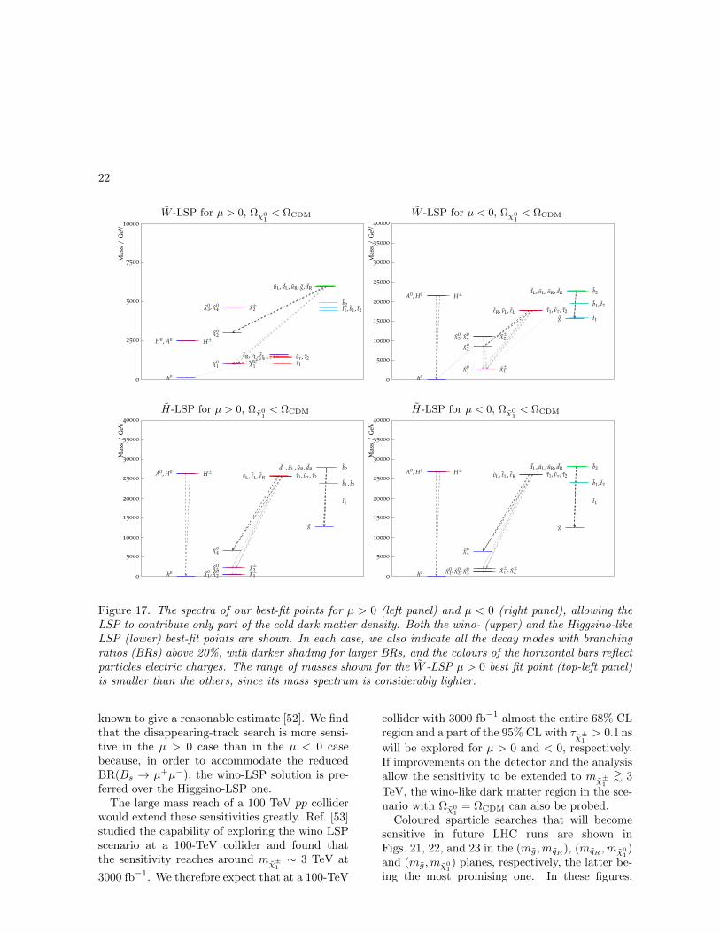
Finally, Fig. 17 displays the spectra of our best-

fit points in the case that the LSP contributesonly a fraction of the cold dark matter density. Aspreviously, the left panels are for µ > 0 and theright panels are for µ < 0 (note the different scaleson the vertical axes). Both the wino- (upper) andthe Higgsino-like LSP (lower) best-fit points areshown. In each case, we also indicate all the decaymodes with branching ratios above 20%.

5.3. χ2 Likelihood Functions for Observ-ables

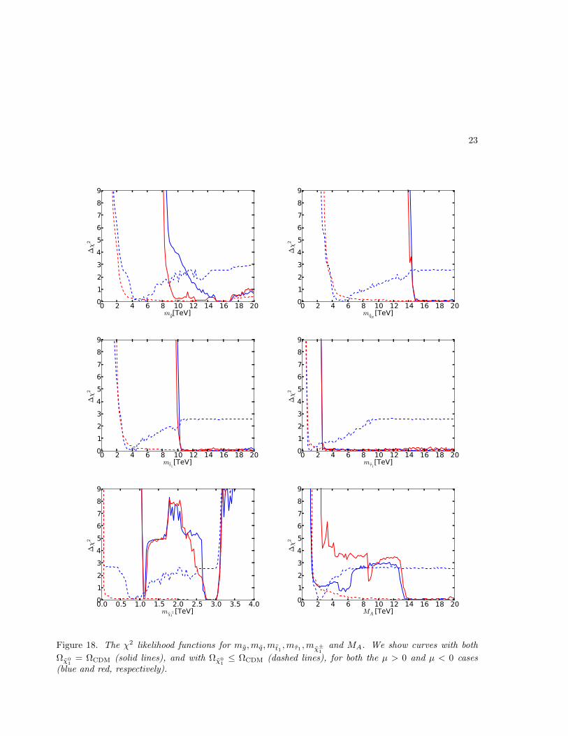
We show in Fig. 18 the one-dimensional like-lihoods for several sparticle masses. In all casesthe solid lines correspond to the case in whichthe LSP accounts for all of the CDM, and thedashed lines for the case in which it may provideonly a fraction of the CDM. The blue lines are forµ > 0 and the red lines are for µ < 0. It is ap-parent that in the all-CDM case the sparticles inthe mAMSB are expected to be too heavy to beproduced at the LHC: mg,mt1

& 10 TeV,mq &15 TeV,mτ1 & 3 TeV,mχ0

1& 1 TeV. However,

in the part-CDM case the sparticle masses may bemuch lighter, with strongly-interacting sparticlespossibly as light as ∼ 2 TeV and much lighter χ0

3

and χ±2 also possible, so that some of them may

become accessible at LHC energies. Indeed, as wediscuss below, future LHC runs should be able toexplore parts of the allowed parameter space.

As shown in Fig 19, there are some interest-

19

0 10 20 30 40 50m0 [TeV]

0

200

400

600

800

1000

1200

1400

m3/2

[TeV

]


µ > 0, Ωχ01< ΩCDM

0 10 20 30 40 50m0 [TeV]

0

200

400

600

800

1000

1200

1400

m3/2

[TeV

]


µ < 0, Ωχ01< ΩCDM

0 10 20 30 40 50tanβ

0

200

400

600

800

1000

1200

1400

m3/

2[TeV

]



0 10 20 30 40 50tanβ

0

200

400

600

800

1000

1200

1400

m3/

2[TeV

]



Figure 13. The (m0,m3/2) planes (upper panels) and the (tanβ,m3/2) planes (lower panels) for µ > 0(left panels) and for µ < 0 (right panels), allowing the χ0

1 to contribute only part of the CDM density.The shadings are the same as in Fig. 4.

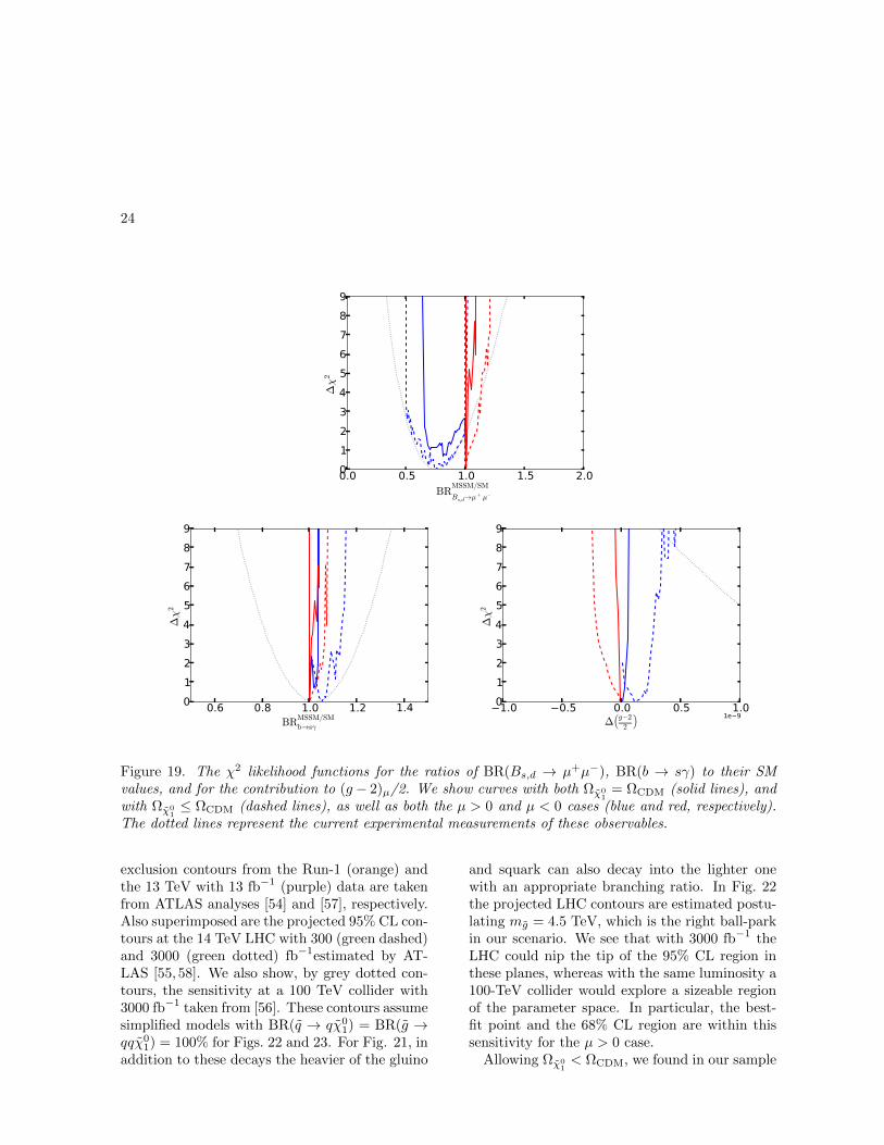
ing prospects for indirect searches for mAMSB ef-fects. There are in general small departures fromthe SM if the LSP accounts for all of the CDM,whereas much more significant effects can ariseif the CDM constraint is relaxed. In particular,we find that significant destructive interferencebetween mAMSB effects and the SM may causea sizeable decrease of the BR(Bs,d → µ+µ−)branching ratio in the positive µ case, which canbe significant within the range of model param-eters allowed at the 2-σ level and improves theagreement with the experimental measurementshown by the dotted line. This effect arises froma region of parameter space at large tanβ whereMA can be below 5 TeV, as seen in the bot-

tom right panel of Fig 18. We find that the de-structive interference in BR(Bs,d → µ+µ−) is al-ways accompanied by a constructive interferencein BR(b → sγ). There is also some possibilityof positive interference in BR(Bs,d → µ+µ−) andnegative interference in BR(b → sγ) when µ < 0and the LSP does not provide all the dark mat-ter, though this effect is much smaller. Finally,we also note that only small effects at the level of10−10 can appear in (g− 2)µ, for either sign of µ.

5.4. Discovery Prospects at the LHC andFCC-hh

As mentioned above, current LHC searchesare not sensitive to the high-mass spectrum ofmAMSB, even if the LSP is not the only compo-

20


0 2 4 6 8 10 12 14 16 18 20MA [TeV]

0

10

20

30

40

50

tanβ



Figure 14. The (MA, tanβ) planes for µ > 0 (left panel) and for µ < 0 (right panel), allowing the χ01 to

contribute only part of the CDM density. The shadings are the same as in Fig. 4.

0.0 0.5 1.0 1.5 2.0 2.5 3.0 3.5 4.0mχ0

1[TeV]

0.000.020.040.060.080.100.120.140.160.18

Ωχ

0 1h

2



0.0 0.5 1.0 1.5 2.0 2.5 3.0 3.5 4.0mχ0

1[TeV]

0.000.020.040.060.080.100.120.140.160.18

Ωχ

0 1h

2



Figure 15. The (mχ01,Ωχ0

1h2) planes in the mAMSB for µ > 0 (left) and µ < 0 (right), allowing the χ0

1 tocontribute only part of the CDM density. The red (blue) contours represent the 68% (95%) CL contours.The shadings are the same as in Fig. 4.

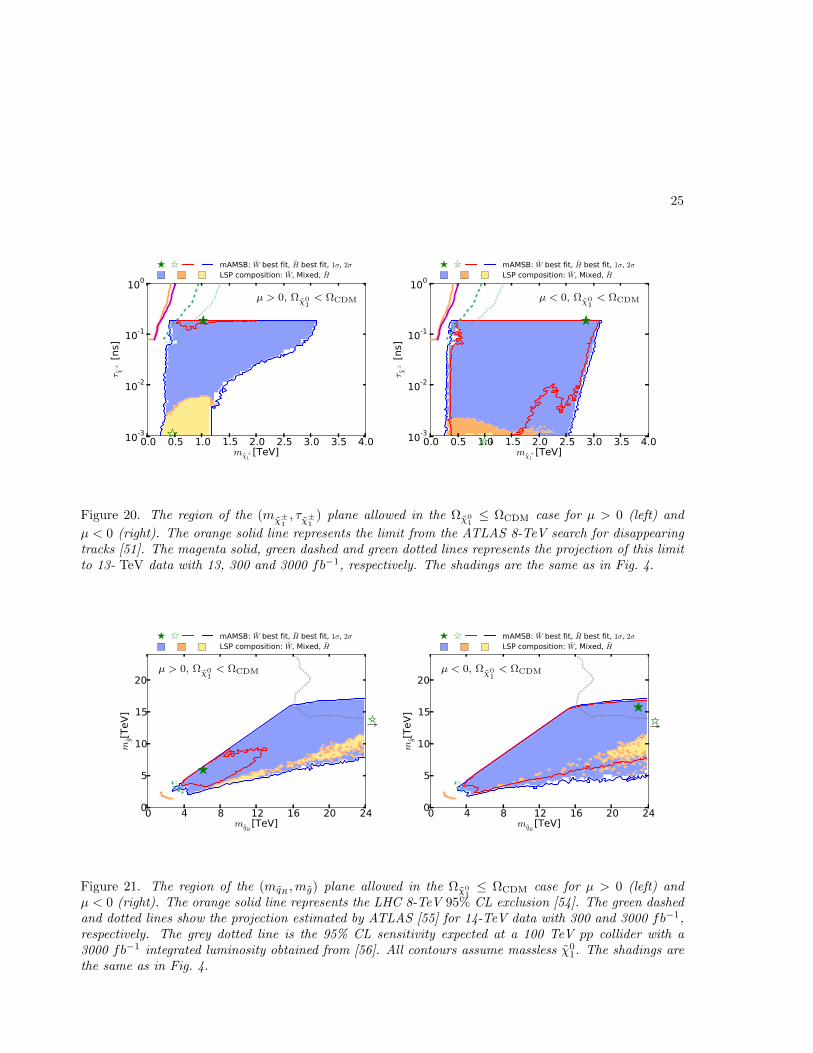
nent of CDM. However, simple extrapolation in-dicates that there are better prospects for futureLHC searches with 300 or 3000 fb−1. Searches forchargino tracks disappearing in the tracker, suchas that performed by ATLAS [51] start to be sen-sitive with 300 fb−1of data, and become muchmore sensitive with 3000 fb−1, as shown in Fig-ure 20. We have obtained the projected contours

for the 13 TeV LHC with 13, 300 and 3000 fb−1byrescaling the Run-1 sensitivity presented in [51].In doing so, at a given lifetime we shift the Run-1value of the 95% CL reach for the wino mass tothe higher value at which the wino cross-sectiontimes luminosity (13, 300 and 3000 fb−1) at the13-TeV LHC coincides with the reach achievedduring Run-1. This method is often used and is

21


2mχ 0

3mχ 0

4mχ ±

1mχ ±

2meL

meRmµL

mµRmτ1

mτ2mqL

mqRmt1

mt2mb1

mb2mg

0.1

1.0

10.0

Part

icle

Mas

ses

[TeV

]

W -LSP for µ > 0, Ωχ01< ΩCDM


2mχ 0

3mχ 0

4mχ ±

1mχ ±

2meL

meRmµL

mµRmτ1

mτ2mqL

mqRmt1

mt2mb1

mb2mg

0.1

1.0

10.0

Part

icle

Mas

ses

[TeV

]

W -LSP for µ < 0, Ωχ01< ΩCDM


2mχ 0

3mχ 0

4mχ ±

1mχ ±

2meL

meRmµL

mµRmτ1

mτ2mqL

mqRmt1

mt2mb1

mb2mg

0.1

1.0

10.0

Part

icle

Mas

ses

[TeV

]

H-LSP for µ > 0, Ωχ01< ΩCDM


2mχ 0

3mχ 0

4mχ ±

1mχ ±

2meL

meRmµL

mµRmτ1

mτ2mqL

mqRmt1

mt2mb1

mb2mg

0.1

1.0

10.0

Part

icle

Mas

ses

[TeV

]

H-LSP for µ < 0, Ωχ01< ΩCDM

Figure 16. The ranges of masses obtained for the wino-like LSP case with µ > 0 (top panel) and µ < 0(second panel), and also for the Higgsino-like LSP case for µ > 0 (third panel) and µ < 0 (bottom panel),relaxing the assumption that the LSP contributes all the cold dark matter density. The one- and two-σCL regions are shown in dark and light orange respectively, and the best-fit values are represented by bluelines.

22

0

2500

5000

7500

10000

Mas

s/

GeV

h0

H0, A0 H±

uL, dL, uR, g, dR

t1, b1, t2

˜R, νL, ˜Lτ1

ντ , τ2χ0

1

χ02

χ±1

χ03, χ0

4 χ±2

b2

W -LSP for µ > 0, Ωχ01< ΩCDM

0

5000

10000

15000

20000

25000

30000

35000

40000

Mas

s/

GeV

h0


b1, t2

t1

˜R, νL, ˜L τ1, ντ , τ2g

χ01

χ02

χ±1

χ03, χ0

4 χ±2

b2

W -LSP for µ < 0, Ωχ01< ΩCDM

0

5000

10000

15000

20000

25000

30000

35000

40000

Mas

s/

GeV

h0


b1, t2

t1

νL, ˜L, ˜R τ1, ντ , τ2

g

χ01, χ0

2 χ±1

χ03

χ04

χ±2

b2

H-LSP for µ > 0, Ωχ01< ΩCDM

0

5000

10000

15000

20000

25000

30000

35000

40000

Mas

s/

GeV

h0


b1, t2

t1

νL, ˜L, ˜R τ1, ντ , τ2

g

χ01, χ0

2, χ03 χ±

1 , χ±2

χ04

b2

H-LSP for µ < 0, Ωχ01< ΩCDM

Figure 17. The spectra of our best-fit points for µ > 0 (left panel) and µ < 0 (right panel), allowing theLSP to contribute only part of the cold dark matter density. Both the wino- (upper) and the Higgsino-likeLSP (lower) best-fit points are shown. In each case, we also indicate all the decay modes with branchingratios (BRs) above 20%, with darker shading for larger BRs, and the colours of the horizontal bars reflectparticles electric charges. The range of masses shown for the W -LSP µ > 0 best fit point (top-left panel)is smaller than the others, since its mass spectrum is considerably lighter.

known to give a reasonable estimate [52]. We findthat the disappearing-track search is more sensi-tive in the µ > 0 case than in the µ < 0 casebecause, in order to accommodate the reducedBR(Bs → µ+µ−), the wino-LSP solution is pre-ferred over the Higgsino-LSP one.

The large mass reach of a 100 TeV pp colliderwould extend these sensitivities greatly. Ref. [53]studied the capability of exploring the wino LSPscenario at a 100-TeV collider and found thatthe sensitivity reaches around mχ±

1∼ 3 TeV at

3000 fb−1. We therefore expect that at a 100-TeV

collider with 3000 fb−1 almost the entire 68% CLregion and a part of the 95% CL with τχ±

1> 0.1 ns

will be explored for µ > 0 and < 0, respectively.If improvements on the detector and the analysisallow the sensitivity to be extended to mχ±

1

>∼ 3

TeV, the wino-like dark matter region in the sce-nario with Ωχ0

1= ΩCDM can also be probed.

Coloured sparticle searches that will becomesensitive in future LHC runs are shown inFigs. 21, 22, and 23 in the (mg,mqR), (mqR ,mχ0

1)

and (mg,mχ01) planes, respectively, the latter be-

ing the most promising one. In these figures,

23

0 2 4 6 8 10 12 14 16 18 20mg[TeV]

0123456789

∆χ

2

0 2 4 6 8 10 12 14 16 18 20mqR

[TeV]0123456789

∆χ

2

0 2 4 6 8 10 12 14 16 18 20mt1

[TeV]0123456789

∆χ

2

0 2 4 6 8 10 12 14 16 18 20mτ1

[TeV]0123456789

∆χ

2

0.0 0.5 1.0 1.5 2.0 2.5 3.0 3.5 4.0mχ±1

[TeV]0123456789

∆χ

2

0 2 4 6 8 10 12 14 16 18 20MA [TeV]

0123456789

∆χ

2

Figure 18. The χ2 likelihood functions for mg,mq,mt1,mτ1 ,mχ±

1and MA. We show curves with both

Ωχ01

= ΩCDM (solid lines), and with Ωχ01≤ ΩCDM (dashed lines), for both the µ > 0 and µ < 0 cases

(blue and red, respectively).

24

0.0 0.5 1.0 1.5 2.0BR

MSSM/SM

Bs,d→µ+ µ−

0123456789

∆χ

2

0.6 0.8 1.0 1.2 1.4BR

MSSM/SM

b→sγ

0123456789

∆χ

2

1.0 0.5 0.0 0.5 1.0∆(g−2

2

) 1e 9

0123456789

∆χ

2

Figure 19. The χ2 likelihood functions for the ratios of BR(Bs,d → µ+µ−), BR(b → sγ) to their SMvalues, and for the contribution to (g− 2)µ/2. We show curves with both Ωχ0

1= ΩCDM (solid lines), and

with Ωχ01≤ ΩCDM (dashed lines), as well as both the µ > 0 and µ < 0 cases (blue and red, respectively).

The dotted lines represent the current experimental measurements of these observables.

exclusion contours from the Run-1 (orange) andthe 13 TeV with 13 fb−1 (purple) data are takenfrom ATLAS analyses [54] and [57], respectively.Also superimposed are the projected 95% CL con-tours at the 14 TeV LHC with 300 (green dashed)and 3000 (green dotted) fb−1estimated by AT-LAS [55, 58]. We also show, by grey dotted con-tours, the sensitivity at a 100 TeV collider with3000 fb−1 taken from [56]. These contours assumesimplified models with BR(q → qχ0

1) = BR(g →qqχ0

1) = 100% for Figs. 22 and 23. For Fig. 21, inaddition to these decays the heavier of the gluino

and squark can also decay into the lighter onewith an appropriate branching ratio. In Fig. 22the projected LHC contours are estimated postu-lating mg = 4.5 TeV, which is the right ball-parkin our scenario. We see that with 3000 fb−1 theLHC could nip the tip of the 95% CL region inthese planes, whereas with the same luminosity a100-TeV collider would explore a sizeable regionof the parameter space. In particular, the best-fit point and the 68% CL region are within thissensitivity for the µ > 0 case.

Allowing Ωχ01< ΩCDM, we found in our sample

25

0.0 0.5 1.0 1.5 2.0 2.5 3.0 3.5 4.0mχ±1

[TeV]10-3

10-2

10-1

100

τ χ± [n

s]



0.0 0.5 1.0 1.5 2.0 2.5 3.0 3.5 4.0mχ±1

[TeV]10-3

10-2

10-1

100

τ χ± [n

s]



Figure 20. The region of the (mχ±1, τχ±

1) plane allowed in the Ωχ0

1≤ ΩCDM case for µ > 0 (left) and

µ < 0 (right). The orange solid line represents the limit from the ATLAS 8-TeV search for disappearingtracks [51]. The magenta solid, green dashed and green dotted lines represents the projection of this limitto 13- TeV data with 13, 300 and 3000 fb−1, respectively. The shadings are the same as in Fig. 4.

0 4 8 12 16 20 24mqR

[TeV]0

5

10

15

20

mg[T

eV]



0 4 8 12 16 20 24mqR

[TeV]0

5

10

15

20

mg[T

eV]



Figure 21. The region of the (mqR ,mg) plane allowed in the Ωχ01≤ ΩCDM case for µ > 0 (left) and

µ < 0 (right). The orange solid line represents the LHC 8-TeV 95% CL exclusion [54]. The green dashedand dotted lines show the projection estimated by ATLAS [55] for 14-TeV data with 300 and 3000 fb−1,respectively. The grey dotted line is the 95% CL sensitivity expected at a 100 TeV pp collider with a3000 fb−1 integrated luminosity obtained from [56]. All contours assume massless χ0

1. The shadings arethe same as in Fig. 4.

26

0 2 4 6 8 10mqR

[TeV]0

1

2

3

4

5

mχ

0 1[T

eV]



0 2 4 6 8 10mqR

[TeV]0

1

2

3

4

5

mχ

0 1[T

eV]



Figure 22. The region of the (mqR ,mχ01) plane allowed in the Ωχ0

1≤ ΩCDM case for µ > 0 (left) and µ < 0

(right). The purple solid line represents the ATLAS 13-TeV 95% CL exclusion using 13 fb−1 of data[57]. The green dashed and dotted lines show the projected 95% CL sensitivity estimated by ATLAS [58]for 14-TeV data with integrated luminosities of 300 and 3000 fb−1, respectively. The grey dotted line isthe 95% CL sensitivity expected at a 100 TeV pp collider with a 3000 fb−1 integrated luminosity obtainedfrom [56]. All contours assume a simplified model with 100% BR for q → qχ0

1. The current limit and100 TeV projection assumes decoupled gluino, while the projection to the higher luminosity LHC assumesa 4.5-TeV gluino. The shadings are the same as in Fig. 4.

very light winos as well as Higgsinos. If both ofthem are light but with a sufficiently large masshierarchy between them, the LHC and a 100-TeVcollider may be able to detect the production of aheavier state decaying subsequently into the light-est state by emitting the heavy bosons W±, Zand h. In Fig. 24 we plot the current and futureLHC reaches as well as the sensitivity expected ata 100-TeV collider with the same luminosity as-sumptions as in the previous figures. The currentlimit (purple) and projected sensitivity (green)at the LHC are estimated by CMS [59] and AT-LAS [58] and assume wino-like chargino and neu-tralino production and a 100% rate for decay intothe W±Z + /ET final state. As can be seen inFig. 24, the region that can be explored is mainlythe Higgsino-like LSP region, whereas we are in-terested in the wino-like chargino and neutralinoproduction. However, unlike the simplified modelassumption employed by ATLAS and CMS, thecharged wino decays into neutral or charged Hig-gsinos emitting W±, Z and h with 50, 25 and

25% branching ratio, respectively [60–62]. Simi-larly, the branching ratios of the neutral wino are50, 25 and 25% for decays into W±, Z and h,respectively. In total, only 25% of the associatedcharged and neutral wino production events con-tribute to the W±Z+/ET channel. The LHC con-tours shown in Fig. 24 should be considered withthis caveat. Also shown by the grey dotted lineis the sensitivity expected at a 100-TeV colliderwith 3000 fb−1 luminosity studied in [60] (seealso [62]) assuming a Higgsino-like LSP and wino-like chargino and neutralino production, takinginto account the correct branching ratios men-tioned above. As can be seen, a 100-TeV collideris sensitive up to mχ0

3∼ 2 TeV, and a large part

of the 95% CL region would be within reach, andalso a substantial portion of the 68% CL regionif µ < 0, though not the best-fit point for eithersign of µ.

Finally, in Fig. 25 we show the (mg,mqR) planefor the scenario with Ωχ0

1= ΩCDM. We found

that a small part of the wino-like dark matter

27

0 4 8 12mg[TeV]

0

1

2

3

4

5

mχ

0 1[T

eV]



0 4 8 12mg[TeV]

0

1

2

3

4

5

mχ

0 1[T

eV]



Figure 23. The region of the (mg,mχ01) plane allowed in the Ωχ0


(right). The purple solid line represents the ATLAS 13-TeV 95% CL exclusion with the data with 13 fb−1

[57]. The green dashed and dotted lines show the projected 95% CL sensitivity estimated by ATLAS [58]for 14-TeV data with integrated luminosities of 300 and 3000 fb−1, respectively. The grey dotted line isthe 95% CL sensitivity expected at a 100 TeV pp collider with a 3000 fb−1 integrated luminosity obtainedfrom [56]. All contours assume a simplified model with 100% BR for g → qqχ0

1. The shadings are thesame as in Fig. 4.

0.0 0.5 1.0 1.5 2.0 2.5 3.0mχ0

3[TeV]

0.0

0.5

1.0

1.5

2.0

mχ

0 1[T

eV]



0.0 0.5 1.0 1.5 2.0 2.5 3.0mχ0

3[TeV]

0.0

0.5

1.0

1.5

2.0

mχ

0 1[T

eV]



Figure 24. The region of the (mχ03,mχ0

1) plane allowed in the Ωχ0


(right). The purple solid line represents the CMS 13-TeV 95% CL exclusion [59] assuming a simplifiedmodel with wino-like chargino and neutralino production and 100% BR for the W±Z+/ET final state. Thegreen dashed (dotted) line shows the projected sensitivity for 14-TeV data with an integrated luminosity of300 fb−1 (3000 fb−1) estimated by ATLAS [58]. The grey dotted line is the 95% CL sensitivity expectedat a 100 TeV pp collider with a 3000 fb−1 integrated luminosity obtained from [60]. The shadings arethe same as in Fig. 4.

28

0 4 8 12 16 20 24mqR

[TeV]0

5

10

15

20

mg[T

eV]


µ > 0, Ωχ01

= ΩCDM

0 4 8 12 16 20 24mqR

[TeV]0

5

10

15

20

mg[T

eV]


µ < 0, Ωχ01

= ΩCDM

Figure 25. The region of the (mqR ,mg) plane allowed in the Ωχ01

= ΩCDM case for µ > 0 (left) andµ < 0 (right). The orange solid line represents the LHC 8-TeV 95% CL exclusion [54]. The green dashedand dotted lines show the projection estimated by ATLAS [55] for 14-TeV data with 300 and 3000 fb−1,respectively. The grey dotted line is the 95% CL sensitivity expected at a 100 TeV pp collider with a3000 fb−1 integrated luminosity obtained from [56]. All contours assume massless χ0

1. The shadings arethe same as in Fig. 4.

region and a good amount of the Higgsino-likedark matter region are within the 95% CL sensi-tivity region at a 100-TeV collider with 3000 fb−1.In particular, the sensitivity contour reaches thebest-fit point for the µ > 0 case.

5.5. Prospects for Direct Detection ofDark Matter

While the heavy spectra of mAMSB modelsmay lie beyond the reach of the LHC constraints,future direct DM search experiments may be ca-pable of detecting the interaction of a mAMSBneutralino, even if it does not provide all theCDM density [63]. Fig 26 displays the cross sec-tion for spin-independent scattering on a proton,σSIp , versus the neutralino mass. As previously,

the left plane is for µ > 0, the right plane is forµ < 0, the 1 and 2σ CL contours are shown as redand blue lines, and the wino- and Higgsino-LSPregions are shaded in pale blue and yellow. Thepale-green-shaded region represents the range ofσSIp excluded at the 95% CL by our combination of

the latest PandaX and LUX results [64,65], whilethe purple and blue lines show the prospective

sensitivities of the LUX-Zeplin (LZ), XENON1Tand XENONnT experiments [66,67]. Also shown,as a dashed orange line, is the neutrino ‘floor’,below which astrophysical neutrino backgroundswould dominate any DM signal [68] (grey region).The mAMSB region allowed at the 2σ level in-cludes points where σSI

p is nominally larger thanthat excluded by LUX and PandaX at the 95%CL, which become allowed when the large theo-retical uncertainty in σSI

p is taken into account.This uncertainty stems largely from the un-

certainty in the strangeness contribution to thenucleon, which receives contributions from twosources. The strange scalar density can be writ-ten as y = 1− σ0/ΣπN where σ0 is the change inthe nucleon mass due to the non-zero u, d quarkmasses, and is estimated from octet baryon massdifferences to be σ0 = 36 ± 7 MeV [69]. Thisis the dominant source of error in the computedcross section. In addition, the π-nucleon Σ termis taken as 50 ± 8 MeV. Another non-negligiblesource of error comes from the uncertainty inquark masses. The resulting 68% CL uncertaintyin the calculated value of σSI

p is more than 50%.

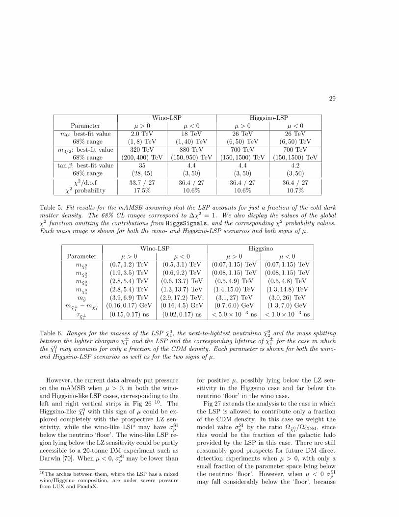
29

Wino-LSP Higgsino-LSPParameter µ > 0 µ < 0 µ > 0 µ < 0

m0: best-fit value 2.0 TeV 18 TeV 26 TeV 26 TeV68% range (1, 8) TeV (1, 40) TeV (6, 50) TeV (6, 50) TeV

m3/2: best-fit value 320 TeV 880 TeV 700 TeV 700 TeV68% range (200, 400) TeV (150, 950) TeV (150, 1500) TeV (150, 1500) TeV

tanβ: best-fit value 35 4.4 4.4 4.268% range (28, 45) (3, 50) (3, 50) (3, 50)

χ2/d.o.f 33.7 / 27 36.4 / 27 36.4 / 27 36.4 / 27χ2 probability 17.5% 10.6% 10.6% 10.7%

Table 5. Fit results for the mAMSB assuming that the LSP accounts for just a fraction of the cold darkmatter density. The 68% CL ranges correspond to ∆χ2 = 1. We also display the values of the globalχ2 function omitting the contributions from HiggsSignals, and the corresponding χ2 probability values.Each mass range is shown for both the wino- and Higgsino-LSP scenarios and both signs of µ.

Wino-LSP HiggsinoParameter µ > 0 µ < 0 µ > 0 µ < 0

mχ01

(0.7, 1.2) TeV (0.5, 3.1) TeV (0.07, 1.15) TeV (0.07, 1.15) TeV

mχ02

(1.9, 3.5) TeV (0.6, 9.2) TeV (0.08, 1.15) TeV (0.08, 1.15) TeV

mχ03

(2.8, 5.4) TeV (0.6, 13.7) TeV (0.5, 4.9) TeV (0.5, 4.8) TeV

mχ04

(2.8, 5.4) TeV (1.3, 13.7) TeV (1.4, 15.0) TeV (1.3, 14.8) TeV

mg (3.9, 6.9) TeV (2.9, 17.2) TeV, (3.1, 27) TeV (3.0, 26) TeVmχ±

1−mχ0

1(0.16, 0.17) GeV (0.16, 4.5) GeV (0.7, 6.0) GeV (1.3, 7.0) GeV

τχ±1

(0.15, 0.17) ns (0.02, 0.17) ns < 5.0× 10−3 ns < 1.0× 10−3 ns

Table 6. Ranges for the masses of the LSP χ01, the next-to-lightest neutralino χ0

2 and the mass splittingbetween the lighter chargino χ±

1 and the LSP and the corresponding lifetime of χ±1 for the case in which

the χ01 may accounts for only a fraction of the CDM density. Each parameter is shown for both the wino-

and Higgsino-LSP scenarios as well as for the two signs of µ.

However, the current data already put pressureon the mAMSB when µ > 0, in both the wino-and Higgsino-like LSP cases, corresponding to theleft and right vertical strips in Fig 26 10. TheHiggsino-like χ0

1 with this sign of µ could be ex-plored completely with the prospective LZ sen-sitivity, while the wino-like LSP may have σSI

p

below the neutrino ‘floor’. The wino-like LSP re-gion lying below the LZ sensitivity could be partlyaccessible to a 20-tonne DM experiment such asDarwin [70]. When µ < 0, σSI

p may be lower than

10The arches between them, where the LSP has a mixedwino/Higgsino composition, are under severe pressurefrom LUX and PandaX.

for positive µ, possibly lying below the LZ sen-sitivity in the Higgsino case and far below theneutrino ‘floor’ in the wino case.

Fig 27 extends the analysis to the case in whichthe LSP is allowed to contribute only a fractionof the CDM density. In this case we weight themodel value σSI

p by the ratio Ωχ01/ΩCDM, since

this would be the fraction of the galactic haloprovided by the LSP in this case. There are stillreasonably good prospects for future DM directdetection experiments when µ > 0, with only asmall fraction of the parameter space lying belowthe neutrino ‘floor’. However, when µ < 0 σSI

p

may fall considerably below the ‘floor’, because

30

of cancellations [71] in the scattering matrix ele-ment.

6. Summary

Using the MasterCode framework, we have con-structed in this paper a global likelihood func-tion for the minimal AMSB model and exploredthe constraints imposed by the available data onflavour, electroweak and Higgs observables, aswell as by LHC searches for gluinos via /ET signa-tures. We have also included the constraint im-posed by the cosmological cold dark matter den-sity, which we interpret as either a measurementor an upper limit on the relic LSP density, andsearches for dark matter scattering.

In the all-CDM case, we find that the spec-trum is relatively heavy, with strongly-interactingsparticles weighing & 10 TeV, but much smallermasses are possible if the LSP contributes only afraction of the overall CDM density. In the all-CDM case, the LSP composition may be eitherwino- or Higgsino-like with almost equal likeli-hood, weighing ∼ 3 TeV and ∼ 1 TeV, respec-tively. On the other hand, in the part-CDM casemuch lighter LSP masses are allowed at the 68%CL, as are intermediate LSP masses.

Because of the high masses in the all-CDMcase, the prospects for discovering sparticlesat the LHC are small, and there are limitedprospects for observing significant deviations forthe SM predictions for flavour observables. How-ever, in the part-CDM case some sparticlesmay well be within reach of the LHC, andthere are more interesting possibilities for observ-ing mAMSB effects on flavour observables, e.g.,BR(Bs,d → µ+µ−). In both cases, wide rangesof dark matter scattering cross-sections, σSI

p are

allowed: σSIp may be very close to the upper lim-

its established recently by the PandaX and LUXexperiments, or it may be within reach of theplanned LUX-Zeplin experiment, or it may evenbe far below the neutrino ‘floor’.

The mAMSB scenario discussed in this pa-per clearly presents different challenges from themodels with GUT-scale unification of (at leastsome of) the soft SUSY-breaking parameters thatwe have studied previously [1–3, 5, 6], and does

not share the flexibility of pMSSM models [4,72].As such, the mAMSB serves as a useful reminderthat SUSY phenomenology may differ signifi-cantly from what is preferred in these other sce-narios.

AcknowledgementsThe work of E.B. and G.W. is supported in part

by the Collaborative Research Center SFB676 ofthe DFG, “Particles, Strings and the early Uni-verse”, and by the European Commission throughthe “HiggsTools” Initial Training Network PITN-GA-2012-316704.The work of R.C. is supportedin part by the National Science Foundation un-der Grant No. PHY-1151640 at the Univer-sity of Illinois Chicago and in part by Fermi-lab, operated by Fermi Research Alliance, LLCunder Contract No. De-AC02-07CH11359 withthe United States Department of Energy. Thiswork of M.J.D. is supported in part by the Aus-tralian Research Council. The work of J.E. issupported in part by STFC (UK) via the re-search grant ST/L000326/1, and the work of H.F.is also supported in part by STFC (UK). Thework of S.H. is supported in part by CICYT(grant FPA 2013-40715-P) and by the SpanishMICINN’s Consolider-Ingenio 2010 Program un-der grant MultiDark CSD2009-00064. The workof D.M.-S. is supported by the European Re-search Council via Grant BSMFLEET 639068.The work of F.L. is supported by World PremierInternational Research Center Initiative (WPI),MEXT, Japan. The work of K.A.O. is sup-ported in part by DOE grant DE-SC0011842at the University of Minnesota. KS is sup-ported by STFC through the IPPP grant. Thework of K.S. is partially supported by the Na-tional Science Centre, Poland, under researchgrants DEC-2014/15/B/ST2/02157 and DEC-2015/18/M/ST2/00054.

31

100 101 102 103 104

mχ01[GeV]

10-5010-4910-4810-4710-4610-4510-4410-4310-42

σSI

p[c

m2

]

XENON100

LUX

PandaX-II + LUX

XENON1T

LZ

XENONnT

neutrino floor


µ > 0, Ωχ01

= ΩCDM

100 101 102 103 104

mχ01[GeV]

10-5010-4910-4810-4710-4610-4510-4410-4310-42

σSI

p[c

m2

]

XENON100

LUX

PandaX-II + LUX

XENON1T

LZ

XENONnT

neutrino floor


µ < 0, Ωχ01

= ΩCDM

Figure 26. The (mχ01, σSIp ) planes in the mAMSB for µ > 0 (left) and µ < 0 (right) in the case when the

LSP accounts for the whole DM density. The red and blue solid lines are the 1 and 2σ CL contours, andthe solid purple and blue lines show the projected 95% exclusion sensitivities of the LUX-Zeplin (LZ) [66]and XENON1T/nT experiments [67], respectively. The green line and shaded region show the combinedlimit from the LUX and PandaX experiments [64,65], and the dashed orange line shows the astrophysicalneutrino ‘floor’ [68], below which astrophysical neutrino backgrounds dominate (grey region). The blue,orange and yellow shadings are the same as in Fig. 4.

100 101 102 103 104

mχ01[GeV]

10-5010-4910-4810-4710-4610-4510-4410-4310-42

σSI

pΩχ

1 0/Ω

CD

M[c

m2

]

XENON100

LUX

PandaX-II + LUX

XENON1T

LZ

XENONnT

neutrino floor



100 101 102 103 104

mχ01[GeV]

10-5010-4910-4810-4710-4610-4510-4410-4310-42

σSI

pΩχ

1 0/Ω

CD

M[c

m2

]

XENON100

LUX

PandaX-II + LUX

XENON1T

LZ

XENONnT

neutrino floor



Figure 27. The (mχ01, σSIp ) planes in the mAMSB for µ > 0 (left) and µ < 0 (right) in the case when the

LSP only accounts for a fraction of the CDM density. The legends, line styles and shadings are the sameas in Fig 26.

32

REFERENCES

1. O. Buchmueller et al., Eur. Phys. J.C 72 (2012) 1878 [arXiv:1110.3568 [hep-ph]]; Eur. Phys. J. C 72 (2012) 2243[arXiv:1207.7315]; Eur. Phys. J. C 74 (2014)2809 [arXiv:1312.5233 [hep-ph]].

2. O. Buchmueller et al., Eur. Phys. J. C 74(2014) 2922 [arXiv:1312.5250 [hep-ph]].

3. O. Buchmueller et al., Eur. Phys. J. C 74(2014) 12, 3212 [arXiv:1408.4060 [hep-ph]].

4. K. J. de Vries et al., Eur. Phys. J. C 75 (2015)no.9, 422 [arXiv:1504.03260 [hep-ph]].

5. E. A. Bagnaschi et al., Eur. Phys. J. C 75(2015) 500 [arXiv:1508.01173 [hep-ph]].

6. E. Bagnaschi et al., arXiv:1610.10084 [hep-ph].

7. For more information and updates, please seehttp://cern.ch/mastercode/.

8. M. Drees and M. M. Nojiri, Phys. Rev.D 47 (1993) 376 [arXiv:hep-ph/9207234];G. L. Kane, C. F. Kolda, L. Roszkowskiand J. D. Wells, Phys. Rev. D 49 (1994)6173 [arXiv:hep-ph/9312272]; H. Baer andM. Brhlik, Phys. Rev. D 53 (1996) 597[arXiv:hep-ph/9508321]; J. R. Ellis, T. Falk,K. A. Olive and M. Schmitt, Phys. Lett.B 388 (1996) 97 [arXiv:hep-ph/9607292];Phys. Lett. B 413 (1997) 355 [arXiv:hep-ph/9705444]; H. Baer and M. Brhlik,Phys. Rev. D 57 (1998) 567 [arXiv:hep-ph/9706509]; J. R. Ellis, T. Falk, G. Ga-nis, K. A. Olive and M. Schmitt, Phys. Rev.D 58 (1998) 095002 [arXiv:hep-ph/9801445];V. D. Barger and C. Kao, Phys. Rev. D 57(1998) 3131 [arXiv:hep-ph/9704403]; J. R. El-lis, T. Falk, G. Ganis and K. A. Olive,Phys. Rev. D 62 (2000) 075010 [arXiv:hep-ph/0004169]; H. Baer, M. Brhlik, M. A. Diaz,J. Ferrandis, P. Mercadante, P. Quintanaand X. Tata, Phys. Rev. D 63 (2001)015007 [arXiv:hep-ph/0005027]; J. R. Ellis,T. Falk, G. Ganis, K. A. Olive and M. Sred-nicki, Phys. Lett. B 510 (2001) 236 [hep-ph/0102098]; L. Roszkowski, R. Ruiz deAustri and T. Nihei, JHEP 0108 (2001)024 [arXiv:hep-ph/0106334]; A. Djouadi,M. Drees and J. L. Kneur, JHEP 0108 (2001)

055 [arXiv:hep-ph/0107316]; U. Chattopad-hyay, A. Corsetti and P. Nath, Phys. Rev.D 66 (2002) 035003 [arXiv:hep-ph/0201001];J. R. Ellis, K. A. Olive and Y. Santoso,New Jour. Phys. 4 (2002) 32 [arXiv:hep-ph/0202110]; H. Baer, C. Balazs, A. Belyaev,J. K. Mizukoshi, X. Tata and Y. Wang, JHEP0207 (2002) 050 [arXiv:hep-ph/0205325];R. Arnowitt and B. Dutta, arXiv:hep-ph/0211417.

9. H. Baer, A. Mustafayev, S. Profumo,A. Belyaev and X. Tata, Phys. Rev. D71 (2005) 095008 [arXiv:hep-ph/0412059];H. Baer, A. Mustafayev, S. Profumo,A. Belyaev and X. Tata, JHEP 0507 (2005)065, hep-ph/0504001; J. R. Ellis, K. A. Oliveand P. Sandick, Phys. Rev. D 78 (2008)075012 [arXiv:0805.2343 [hep-ph]]; J. Ellis,F. Luo, K. A. Olive and P. Sandick, Eur.Phys. J. C 73 (2013) 2403 [arXiv:1212.4476[hep-ph]]; J. Ellis, J. L. Evans, F. Luo, N. Na-gata, K. A. Olive and P. Sandick, Eur. Phys.J. C 76, no. 1, 8 (2016) [arXiv:1509.08838[hep-ph]].

10. J. Ellis, K. Olive and Y. Santoso, Phys. Lett.B 539 (2002) 107 [arXiv:hep-ph/0204192];J. R. Ellis, T. Falk, K. A. Olive andY. Santoso, Nucl. Phys. B 652 (2003) 259[arXiv:hep-ph/0210205].

11. See, for example, C. F. Berger, J. S. Gainer,J. L. Hewett and T. G. Rizzo, JHEP0902, 023 (2009) [arXiv:0812.0980 [hep-ph]]; S. S. AbdusSalam, B. C. Allanach,F. Quevedo, F. Feroz and M. Hobson, Phys.Rev. D 81, 095012 (2010) [arXiv:0904.2548[hep-ph]]; J. A. Conley, J. S. Gainer,J. L. Hewett, M. P. Le and T. G. Rizzo, Eur.Phys. J. C 71, 1697 (2011) [arXiv:1009.2539[hep-ph]]; J. A. Conley, J. S. Gainer,J. L. Hewett, M. P. Le and T. G. Rizzo,[arXiv:1103.1697 [hep-ph]]; B. C. Allanach,A. J. Barr, A. Dafinca and C. Gwenlan, JHEP1107, 104 (2011) [arXiv:1105.1024 [hep-ph]];S. S. AbdusSalam, et al., Eur. Phys. J. C71 (2011) 1835 [arXiv:1109.3859 [hep-ph]];S. Sekmen, S. Kraml, J. Lykken, F. Moort-gat, S. Padhi, L. Pape, M. Pierini andH. B. Prosper et al., JHEP 1202 (2012)

33

075 [arXiv:1109.5119 [hep-ph]]; A. Arbey,M. Battaglia and F. Mahmoudi, Eur. Phys.J. C 72 (2012) 1847 [arXiv:1110.3726 [hep-ph]]; A. Arbey, M. Battaglia, A. Djouadiand F. Mahmoudi, Phys. Lett. B 720 (2013)153 [arXiv:1211.4004 [hep-ph]]; M. W. Cahill-Rowley, J. L. Hewett, A. Ismail andT. G. Rizzo, Phys. Rev. D 88 (2013) 3,035002 [arXiv:1211.1981 [hep-ph]]; C. Strege,G. Bertone, G. J. Besjes, S. Caron, R. Ruizde Austri, A. Strubig and R. Trotta, JHEP1409 (2014) 081 [arXiv:1405.0622 [hep-ph]];M. Cahill-Rowley, J. L. Hewett, A. Ismail andT. G. Rizzo, Phys. Rev. D 91 (2015) 5, 055002[arXiv:1407.4130 [hep-ph]]; L. Roszkowski,E. M. Sessolo and A. J. Williams, JHEP1502, 014 (2015) [arXiv:1411.5214 [hep-ph]]; M. E. Cabrera-Catalan, S. Ando,C. Weniger and F. Zandanel, Phys. Rev. D92, no. 3, 035018 (2015) [arXiv:1503.00599[hep-ph]]; J. Chakrabortty, A. Choudhuryand S. Mondal, JHEP 1507, 038 (2015)[arXiv:1503.08703 [hep-ph]].

12. M. Cannoni, J. Ellis, M. E. Gmez, S. Lola andR. Ruiz de Austri, JCAP 1603, no. 03, 041(2016) [arXiv:1511.06205 [hep-ph]].

13. H. Goldberg, Phys. Rev. Lett. 50 (1983) 1419;J. Ellis, J. Hagelin, D. Nanopoulos, K. Oliveand M. Srednicki, Nucl. Phys. B 238 (1984)453.

14. M. Dine and D. MacIntire, Phys. Rev. D46, 2594 (1992) [hep-ph/9205227]; L. Ran-dall and R. Sundrum, Nucl. Phys. B 557,79 (1999) [arXiv:hep-th/9810155]; G. F. Giu-dice, M. A. Luty, H. Murayama and R. Rat-tazzi, JHEP 9812, 027 (1998) [arXiv:hep-ph/9810442]; A. Pomarol and R. Rattazzi,JHEP 9905, 013 (1999) [hep-ph/9903448];J. A. Bagger, T. Moroi and E. Poppitz, JHEP0004, 009 (2000) [arXiv:hep-th/9911029];P. Binetruy, M. K. Gaillard and B. D. Nel-son, Nucl. Phys. B 604, 32 (2001) [arXiv:hep-ph/0011081].

15. T. Gherghetta, G. Giudice and J. Wells,Nucl. Phys. B 559 (1999) 27 [arXiv:hep-ph/9904378]; E. Katz, Y. Shadmi andY. Shirman, JHEP 9908, 015 (1999) [hep-ph/9906296]; Z. Chacko, M. A. Luty,

I. Maksymyk and E. Ponton, JHEP 0004,001 (2000) [hep-ph/9905390]; J. L. Fengand T. Moroi, Phys. Rev. D 61, 095004(2000) [hep-ph/9907319]; G. D. Kribs, Phys.Rev. D 62, 015008 (2000) [hep-ph/9909376];U. Chattopadhyay, D. K. Ghosh and S. Roy,Phys. Rev. D 62, 115001 (2000) [hep-ph/0006049]; I. Jack and D. R. T. Jones,Phys. Lett. B 491, 151 (2000) [hep-ph/0006116]; H. Baer, J. K. Mizukoshi andX. Tata, Phys. Lett. B 488, 367 (2000)[hep-ph/0007073]; A. Datta, A. Kundu andA. Samanta, Phys. Rev. D 64, 095016 (2001)[hep-ph/0101034]; H. Baer, R. Dermisek,S. Rajagopalan and H. Summy, JCAP 1007,014 (2010) [arXiv:1004.3297 [hep-ph]]; A. Ar-bey, A. Deandrea and A. Tarhini, JHEP1105, 078 (2011) [arXiv:1103.3244 [hep-ph]];B. C. Allanach, T. J. Khoo and K. Saku-rai, JHEP 1111, 132 (2011) [arXiv:1110.1119[hep-ph]]; A. Arbey, A. Deandrea, F. Mah-moudi and A. Tarhini, Phys. Rev. D 87, no.11, 115020 (2013) [arXiv:1304.0381 [hep-ph]].

16. M. Ibe, T. Moroi and T. T. Yanagida,Phys. Lett. B 644, 355 (2007) [hep-ph/0610277]; J. L. Evans, M. Ibe, K. A. Oliveand T. T. Yanagida, Eur. Phys. J. C73, 2468 (2013) [arXiv:1302.5346 [hep-ph]];J. L. Evans, N. Nagata and K. A. Olive, Phys.Rev. D 91, 055027 (2015) [arXiv:1502.00034[hep-ph]].

17. P. A. R. Ade et al. [Planck Collabora-tion], Astron. Astrophys. 594 (2016) A13[arXiv:1502.01589 [astro-ph.CO]].

18. J. Hisano, S. Matsumoto, M. Nagai, O. Saitoand M. Senami, Phys. Lett. B 646 (2007) 34[hep-ph/0610249].

19. M. Cirelli, A. Strumia and M. Tam-burini, Nucl. Phys. B 787 (2007) 152[arXiv:0706.4071 [hep-ph]]; A. Hryczuk,R. Iengo and P. Ullio, JHEP 1103(2011) 069 [arXiv:1010.2172 [hep-ph]];M. Beneke, A. Bharucha, F. Dighera,C. Hellmann, A. Hryczuk, S. Recksiegel andP. Ruiz-Femenia, JHEP 1603 (2016) 119[arXiv:1601.04718 [hep-ph]].

20. A. Sommerfeld, Ann. Phys. 403, (1931) 257.21. G. Aad et al. [ATLAS and CMS Collabora-

34

tions], Phys. Rev. Lett. 114 (2015) 191803[arXiv:1503.07589 [hep-ex]].

22. G. Degrassi, S. Heinemeyer, W. Hollik,P. Slavich and G. Weiglein, Eur. Phys. J. C28 (2003) 133 [arXiv:hep-ph/0212020];

23. P. Bechtle, S. Heinemeyer, O. Stal, T. Ste-faniak and G. Weiglein, Eur. Phys. J. C74 (2014) 2, 2711 [arXiv:1305.1933 [hep-ph]]; JHEP 1411 (2014) 039 [arXiv:1403.1582[hep-ph]].

24. B. C. Allanach, G. Hiller, D. R. T. Jonesand P. Slavich, JHEP 0904 (2009)088 doi:10.1088/1126-6708/2009/04/088[arXiv:0902.4880 [hep-ph]].

25. S. Chatrchyan et al. [CMS Collabora-tion], Phys. Rev. Lett. 111 (2013) 101804[arXiv:1307.5025 [hep-ex]]; R.Aaij et al.[LHCb Collaboration], Phys. Rev. Lett.111 (2013) 101805 [arXiv:1307.5024 [hep-ex]]; V. Khachatryan et al. [CMS andLHCb Collaborations], Nature 522 (2015) 68[arXiv:1411.4413 [hep-ex]]; M. Aaboud et al.[ATLAS Collaboration], Eur. Phys. J. C 76(2016) no.9, 513 [arXiv:1604.04263 [hep-ex]].

26. S. Heinemeyer et al., JHEP 0608 (2006)052 [arXiv:hep-ph/0604147]; S. Heinemeyer,W. Hollik, A. M. Weber and G. Weiglein,JHEP 0804 (2008) 039 [arXiv:0710.2972[hep-ph]].

27. C. Patrignani et al. [Particle Data Group Col-laboration], Chin. Phys. C 40 (2016) 100001doi:10.1088/1674-1137/38/9/090001

28. S. Heinemeyer, W. Hollik and G. Wei-glein, Comput. Phys. Commun. 124 (2000)76 [arXiv:hep-ph/9812320]; S. Heinemeyer,W. Hollik and G. Weiglein, Eur. Phys.J. C 9 (1999) 343 [arXiv:hep-ph/9812472];M. Frank et al., JHEP 0702 (2007) 047[arXiv:hep-ph/0611326]; T. Hahn, S. Heine-meyer, W. Hollik, H. Rzehak and G. Weiglein,Comput. Phys. Commun. 180 (2009) 1426;T. Hahn, S. Heinemeyer, W. Hollik, H. Rze-hak and G. Weiglein, Phys. Rev. Lett. 112(2014) 14, 141801 [arXiv:1312.4937 [hep-ph]].See http://www.feynhiggs.de .

29. P. Bechtle, O. Brein, S. Heinemeyer,G. Weiglein and K. E. Williams, Com-put. Phys. Commun. 181 (2010) 138

[arXiv:0811.4169 [hep-ph]], Comput. Phys.Commun. 182 (2011) 2605 [arXiv:1102.1898[hep-ph]]; P. Bechtle et al., Eur. Phys. J. C74 (2014) 3, 2693 [arXiv:1311.0055 [hep-ph]].

30. P. Bechtle, S. Heinemeyer, O. Stal, T. Ste-faniak and G. Weiglein, Eur. Phys. J. C 75(2015) 9, 421 [arXiv:1507.06706 [hep-ph]].

31. V. Khachatryan et al. [CMS Collaboration],JHEP 1410 (2014) 160 [arXiv:1408.3316[hep-ex]].

32. ATLAS Collaboration, ATLAS-CONF-2016–085.

33. V. Khachatryan et al. [CMS Collaboration],JHEP 1610 (2016) 006 [arXiv:1603.04053[hep-ex]].

34. V. Khachatryan et al. [CMS Collaboration],Eur. Phys. J. C 74 (2014) no.9, 3036[arXiv:1405.7570 [hep-ex]].

35. G. Aad et al. [ATLAS Collaboration], JHEP1405 (2014) 071 [arXiv:1403.5294 [hep-ex]].

36. H. Iminniyaz and M. Kakizaki, Nucl. Phys.B 851 (2011) 57 [arXiv:1008.2905 [astro-ph.CO]].

37. Information about this code is available fromK. A. Olive: it contains important contri-butions from J. Evans, T. Falk, A. Ferstl,G. Ganis, F. Luo, A. Mustafayev, J. McDon-ald, K. A. Olive, P. Sandick, Y. Santoso, V.Spanos, and M. Srednicki.

38. T. Cohen, M. Lisanti, A. Pierce andT. R. Slatyer, JCAP 1310, 061 (2013)[arXiv:1307.4082]; J. Fan and M. Reece,JHEP 1310, 124 (2013) [arXiv:1307.4400[hep-ph]]; A. Hryczuk, I. Cholis, R. Iengo,M. Tavakoli and P. Ullio, JCAP 1407,031 (2014) [arXiv:1401.6212 [astro-ph.HE]];B. Bhattacherjee, M. Ibe, K. Ichikawa,S. Matsumoto and K. Nishiyama, JHEP1407, 080 (2014) [arXiv:1405.4914 [hep-ph]]; M. Baumgart, I. Z. Rothstein andV. Vaidya, JHEP 1504, 106 (2015)[arXiv:1412.8698 [hep-ph]]; M. Beneke,A. Bharucha, A. Hryczuk, S. Recksiegel andP. Ruiz-Femenia, arXiv:1611.00804 [hep-ph].

39. M. Benito, N. Bernal, N. Bozorgnia, F. Caloreand F. Iocco, arXiv:1612.02010 [hep-ph].

40. J. L. Feng, K. T. Matchev and T. Moroi,Phys. Rev. Lett. 84, 2322 (2000) [arXiv:hep-

35

ph/9908309]; Phys. Rev. D 61, 075005(2000) [arXiv:hep-ph/9909334]; J. L. Feng,K. T. Matchev and F. Wilczek, Phys. Lett.B 482, 388 (2000) [arXiv:hep-ph/0004043];H. Baer, T. Krupovnickas, S. Profumo andP. Ullio, JHEP 0510 (2005) 020 [hep-ph/0507282]; J. L. Feng, K. T. Matchevand D. Sanford, Phys. Rev. D 85, 075007(2012) [arXiv:1112.3021 [hep-ph]]; P. Draper,J. Feng, P. Kant, S. Profumo and D. San-ford, Phys. Rev. D 88, 015025 (2013)[arXiv:1304.1159 [hep-ph]].

41. G. Belanger, F. Boudjema, A. Pukhov andA. Semenov, Comput. Phys. Commun. 185(2014) 960 [arXiv:1305.0237 [hep-ph]], andreferences therein.

42. B. C. Allanach, Comput. Phys. Commun. 143(2002) 305 [arXiv:hep-ph/0104145].

43. G. Isidori and P. Paradisi, Phys. Lett.B 639 (2006) 499 [arXiv:hep-ph/0605012];G. Isidori, F. Mescia, P. Paradisi andD. Temes, Phys. Rev. D 75 (2007)115019 [arXiv:hep-ph/0703035], and refer-ences therein.

44. M. Muhlleitner, A. Djouadi, Y. Mambrini,Comput. Phys. Commun. 168 (2005) 46[arXiv:hep-ph/0311167].

45. P. Skands et al., JHEP 0407 (2004) 036[arXiv:hep-ph/0311123]; B. Allanach et al.,Comput. Phys. Commun. 180 (2009) 8[arXiv:0801.0045 [hep-ph]].

46. F. Mahmoudi, Comput. Phys. Commun.178 (2008) 745 [arXiv:0710.2067 [hep-ph]];Comput. Phys. Commun. 180 (2009) 1579[arXiv:0808.3144 [hep-ph]]; D. Eriksson,F. Mahmoudi and O. Stal, JHEP 0811 (2008)035 [arXiv:0808.3551 [hep-ph]].

47. A. Crivellin, J. Rosiek, P. H. Chankowski,A. Dedes, S. Jaeger and P. Tanedo, Com-put. Phys. Commun. 184 (2013) 1004[arXiv:1203.5023 [hep-ph]].

48. Hunter, J. D., Computing In Science & Engi-neering, 9.3 (2007): 90-95

49. A. Buckley, Eur. Phys. J. C 75, no. 10, 467(2015) [arXiv:1305.4194 [hep-ph]].

50. F. Feroz and M.P. Hobson,Mon. Not. Roy. Astron. Soc. 384(2008) 449 [arXiv:0704.3704 [astro-ph]].

F. Feroz, M.P. Hobson and M. Bridges,Mon. Not. Roy. Astron. Soc. 398 (2009)1601-1614 [arXiv:0809.3437 [astro-ph]].F. Feroz, M.P. Hobson, E. Cameron andA.N. Pettitt, [arXiv:1306.2144 [astro-ph]].

51. G. Aad et al. [ATLAS Collaboration],Phys. Rev. D 88 (2013) no.11, 112006[arXiv:1310.3675 [hep-ex]].

52. G. Salam and A. Weiler,http://collider-reach.web.cern.ch/

collider-reach

53. M. Low and L. T. Wang, JHEP 1408 (2014)161 [arXiv:1404.0682 [hep-ph]]; S. A. R. Ellisand B. Zheng, Phys. Rev. D 92 (2015) no.7,075034 [arXiv:1506.02644 [hep-ph]].

54. G. Aad et al. [ATLAS Collaboration], JHEP1409 (2014) 176[arXiv:1405.7875 [hep-ex]].

55. The ATLAS collaboration [ATLAS Collabo-ration], ATL-PHYS-PUB-2012-001.

56. T. Cohen, T. Golling, M. Hance, A. Henrichs,K. Howe, J. Loyal, S. Padhi and J. G. Wacker,JHEP 1404 (2014) 117 [arXiv:1311.6480[hep-ph]].

57. The ATLAS collaboration [ATLAS Collabo-ration], ATLAS-CONF-2016-078.

58. The ATLAS collaboration [ATLAS Collabo-ration], ATL-PHYS-PUB-2014-010.

59. CMS Collaboration [CMS Collaboration],CMS-PAS-SUS-16-024.

60. B. S. Acharya, K. Bozek, C. Pongkiti-vanichkul and K. Sakurai, JHEP 1502 (2015)181 [arXiv:1410.1532 [hep-ph]].

61. S. Jung, JHEP 1406 (2014) 111[arXiv:1404.2691 [hep-ph]].

62. S. Gori, S. Jung, L. T. Wang and J. D. Wells,JHEP 1412 (2014) 108 [arXiv:1410.6287[hep-ph]].

63. C. Cheung, L. J. Hall, D. Pinner andJ. T. Ruderman, JHEP 1305 (2013)100 [arXiv:1211.4873 [hep-ph]]; H. Baer,V. Barger and D. Mickelson, Phys. Lett. B726 (2013) 330[arXiv:1303.3816 [hep-ph]]; D. Barducci,A. Belyaev, A. K. M. Bharucha, W. Porodand V. Sanz, JHEP 1507 (2015) 066[arXiv:1504.02472 [hep-ph]]; M. Badziak,A. Delgado, M. Olechowski, S. Pokorski

36

and K. Sakurai, JHEP 1511 (2015) 053[arXiv:1506.07177 [hep-ph]].

64. A. Tan et al. [PandaX-II Collaboration],Phys. Rev. Lett. 117, no. 12, 121303 (2016)[arXiv:1607.07400 [hep-ex]].

65. D. S. Akerib et al., arXiv:1608.07648 [astro-ph.CO].

66. D. C. Malling, D. S. Akerib, H. M. Araujo,X. Bai, S. Bedikian, E. Bernard, A. Bernsteinand A. Bradley et al., arXiv:1110.0103 [astro-ph.IM].

67. E. Aprile et al. [XENON Collabora-tion], JCAP 1604 (2016) no.04, 027[arXiv:1512.07501 [physics.ins-det]];https://idm2016.shef.ac.uk/indico/

event/0/session/5/contribution/76/

material/slides/0.pdf.68. P. Cushman, C. Galbiati, D. N. McK-

insey, H. Robertson, T. M. P. Tait,D. Bauer, A. Borgland and B. Cabrera et al.,arXiv:1310.8327 [hep-ex].

69. J. Gasser, H. Leutwyler, and M. E. Sainio,Phys. Lett. B253, 252 (1991); M. Knecht,hep-ph/9912443 M. E. Sainio, PiN Newslett.16, 138 (2002) [arXiv:hep-ph/0110413].

70. L. Baudis [DARWIN Consortium Collabora-tion], J. Phys. Conf. Ser. 375 (2012) 012028[arXiv:1201.2402 [astro-ph.IM]].

71. For some discussions of these cancel-lations, see J. R. Ellis, A. Ferstl andK. A. Olive, Phys. Lett. B 481, 304 (2000)[hep-ph/0001005]; V. Mandic, A. Pierce,P. Gondolo and H. Murayama, hep-ph/0008022; J. R. Ellis, J. L. Feng, A. Ferstl,K. T. Matchev and K. A. Olive, Eur. Phys.J. C 24, 311 (2002) [astro-ph/0110225];C. Cheung, L. J. Hall, D. Pinner andJ. T. Ruderman, JHEP 1305, 100 (2013)[arXiv:1211.4873 [hep-ph]]; P. Huang andC.E. M. Wagner, Phys. Rev. D 90, no.1, 015018 (2014) [arXiv:1404.0392 [hep-ph]]; T. Han, F. Kling, S. Su and Y. Wu,[arXiv:1612.02387 [hep-ph]].

72. E. Bagnaschi et al., in preparation.

Likelihood Analysis of the Minimal AMSB Model - PUBDB

Documents

Transcript of Likelihood Analysis of the Minimal AMSB Model - PUBDB