In ICAI'10 - The 2010 International Conference on Artificial Intelligence at the 2010 World Congress in Computer Science Computer Engineering and Applied Computing, Las Vegas, Nevada, July 12-15.

© 2010 HRL Laboratories, LLC, All rights reserved.

Further Explorations of a Minimal Polychronous Memory Mike Howard, Mike Daily, Dave Payton, Yang Chen, and Rashmi Sundareswara

{mdhoward1, mjdaily, dwpayton, ychen, rnsundareswara}@hrl.com

HRL Laboratories, LLC, 3011 Malibu Canyon Rd, Malibu, CA.

Abstract – The study of temporal spiking dynamics in biologically inspired neural networks (polychronous groups discovered by Izhikevich[2]) exhibits complex dynamics that makes it difficult to study. A minimal model of polychronous groups in neural networks was proposed by Maier and Miller [7] who discovered that a very minimal neural network model, without the synaptic weights was sufficient to produce PCGs. In this paper we expand on their study and propose ways to condition the network to produce sets of PCGs that are more unique; hence theoretically more descriptive of an input signal.

Keywords: Polychronous groups, recurrent neural networks, reservoir computing

1 Introduction Although recurrent neural networks have been studied since the 1990’s, there was no practical way to control and use them until around 2000 when Maass and others developed their use, calling them Liquid State Machines (LSM), a branch of Reservoir Computing [5, 6, 11]. [6] provides a theoretical foundation for approximating any biologically relevant computation on spike trains by LSMs. LSMs have a theoretical capacity bounded by N (the number of neurons in the liquid). In practice, their capacity with noisy input is typically below 0.20N. Other associative memories such as Hopfield/Grossberg networks have a theoretical capacity of ~0.14N, but cannot practically be used at this capacity.1

Izhikevich observed that a type of LSM composed of leaky integrator spiking neurons with axonal delays and spike-timing-dependent-

1 Contact author.

plasticity (STDP) can exhibit reproducible temporal firing patterns called polychronous groups (PCGs). STDP trains the synaptic weights so that weights are increased if the presynaptic neuron fires just before the postsynaptic neuron [1]. The Izhikevich model has some features of the mammalian brain such as a 4:1 ratio of excitatory to inhibitory neurons. Surprisingly, it was found that the number of PCGs generated by such a model far exceeds the number of nodes, theoretically approaching N-factorial for N nodes.

A parsimonious hardware memory with such a high capacity would be very attractive. But the Izhikevich model exhibits complex multidimensional dynamics; the interactions between PCGs in context of the dynamic state of the surrounding recurrent neural network are little understood. Basic research is needed to understand how to control such a system for practical use.

Several works [2, 7, 8] have included algorithms for how to find the set of theoretical PCGs that a particular network can generate, and divided them into two types, structural and dynamical. [9, 10] describes an algorithm for supervised training of an output layer for an Izhikevich network to make it into a classification system. They demonstrated that certain subsets of PCGs are characteristic of particular input signals

Recently Maier and Miller [7] explored a “minimal” version of the Izhikevich network that produces similar PCG activity without STDP training or inhibitory neurons. In fact no synaptic weights were required, and the leaky integrator neural model was replaced with an additive voltage model (no leaks). An essential feature of both models is a variety of fixed timing

© 2010 HRL Laboratories, LLC, All rights reserved. 2

delays between neurons. Parametric studies of the Maier and Miller model showed that the number of PCGs in the network increases linearly with the number of neurons, and exponentially with the number of output connections per neuron, in numbers that compare favorably to the Izhikevich model. Our studies confirm this result, as illustrated in Figure 1.

In this paper, we explore these deceptively simple memory models in more detail to get a better understanding of their behavior, and how to control properties of the PCG population such as scalability, uniqueness, network saturation, and superposition.

2 Metrics and Means

2.1 Description of the Model

The neural network consists of N neurons, each of whose outputs are recurrently connected to m of the N. We are studying very small networks of 5 ≤ N ≤ 15. The basic neural node is the same additive voltage node used in [1]: the neuron can fire only if its input links contribute a total of at least 2 mV, and when it fires, 1 mV is added to each of the m output neurons after the delay time of the link. The standard undamped voltage increment is 1 mV per incoming spike, except in the case of a type of damping called voltage dissipation, described in section 2.3.2 below.

We used the procedure outlined in [7] to simulate each PCG. A firing matrix has N rows, one per neuron, and the columns represent time steps in milliseconds. A separate NxN matrix of axonal delays is randomly populated with delays from 1 to dmax (default 5). We employ symmetric delays with 0’s along the diagonal, but non-symmetric delays could be used without changes in our algorithm. Input spikes are injected into the network by recording a voltage of 2mV at each (neuronID, spiketime) entry in the firing matrix. Then the firing matrix is simulated forward in time, left to right, looking for any entry ≥ 2 (a neuron ready to fire). Its m postsynaptic neurons are looked up in the delay matrix, and a voltage increment is added to the appropriate cell (postsynaptic_neuronID, spiketime+delay) for each.

2.2 Experimental Procedures

2.2.1 Scalability We confirmed and extended the scalability results in [7] with a parametric study for networks for 5 ≤ N ≤ 15 and 4 ≤ m ≤ N-1. Ten runs were performed for each combination of N and m, choosing a new connection/delay matrix for each run. The results are compiled in Figure 3 and described in section 3.1.

2.2.2 PCG Uniqueness PCGs that are minimally correlated with other PCGs provide more positive indications of the inputs. For example, Figure 1 shows three different inputs that each cause exactly the same firing pattern. A good metric for PCG correlation is the Levenshtein algorithm [4], also known as edit distance, which is the sum cost of changing one sequence into another using insertion, deletion, and replacement operations.

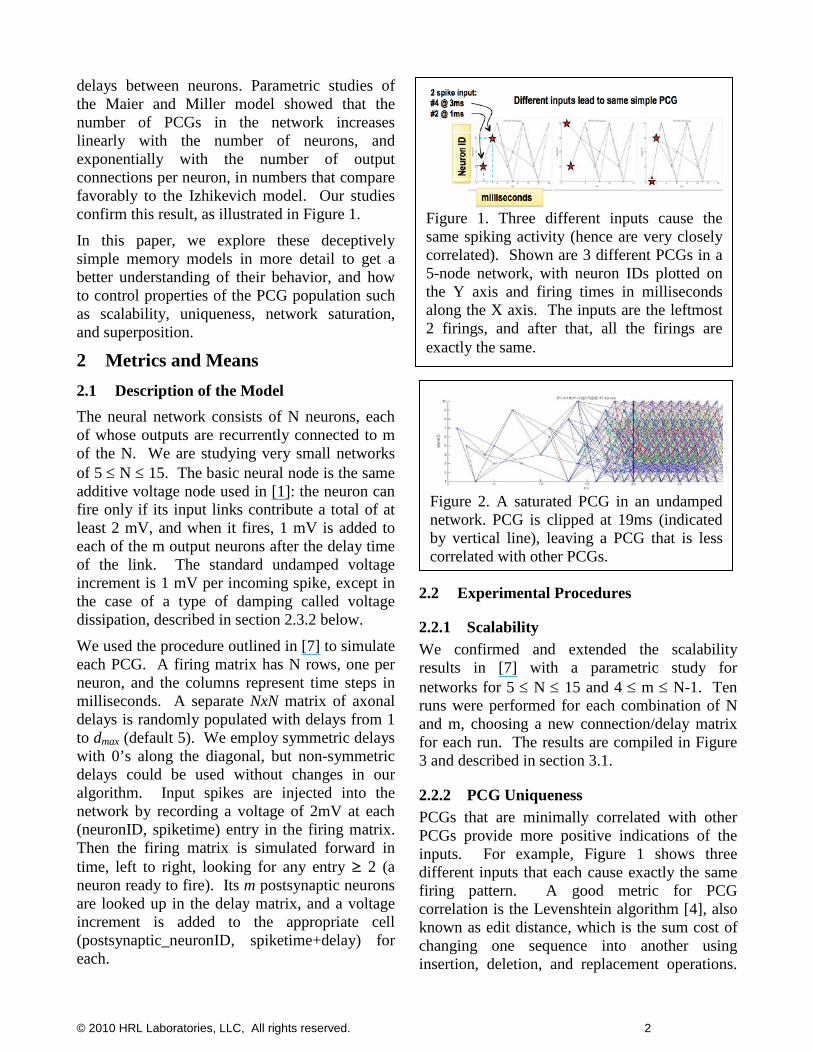
Figure 2. A saturated PCG in an undamped network. PCG is clipped at 19ms (indicated by vertical line), leaving a PCG that is less correlated with other PCGs.

Figure 1. Three different inputs cause the same spiking activity (hence are very closely correlated). Shown are 3 different PCGs in a 5-node network, with neuron IDs plotted on the Y axis and firing times in milliseconds along the X axis. The inputs are the leftmost 2 firings, and after that, all the firings are exactly the same.

© 2010 HRL Laboratories, LLC, All rights reserved. 3

We assigned costs of 1 for each of these operations, treating the firing sequence of neuron IDs as a string. We did not consider the temporal firing delays in our simple metric, although it would be straightforward to incorporate that as well.

We added a discount factor, so it costs more if differences are earlier in the sequence than later. The cost is reduced from 1 for the first character of each PCG string down to 0.1 at the kth character, and from there down to 0 for the last elements of each PCG. This means the discount factor declines steeply to k, and tails off more shallowly from there. Our reasoning is that the earlier firings in a PCG are most characteristic of the inputs.

The results of our uniqueness study are described in section 3.2.

2.2.3 Saturation Without damping, any network will saturate; that is, after some period of time all neurons start firing at once, which looks like an infinite repeating sequence. Biological neurons are modeled using dissipative terms like the leaky integrator used in [2]. Figure 2 shows an example of such saturation in the undamped minimal network described in [7]. The correlation measure for two saturated PCGs that are otherwise very different in the first 10 firings is dominated by the saturated portion. Those PCGs become much more uniquely identifiable if the point of saturation can be detected and the rest of the firings removed from consideration.

We developed a simple procedure to identify a repeating sequence in a PCG by “folding” the sequence of neuron IDs into matrices of different number of columns (using Matlab reshape command) and counting the number of rows that are the same. The repeating sequence appears as the row with the maximum number of repetitions in the overall sequence. Of course, as we try different numbers of columns, there can be several choices for a repeating sequence, so we prefer the longest sequence (up to the number of neurons in the network, N) that repeats more than once; e.g., 10-digit sequence that repeats 18 times

out of 224 firings. For example, to analyze sequence x:

for len=2:N % length of subsequence x2 = reshape(x(1:floor(length(x)/len)*len), len,floor(length(x)/len))'; count number of repeats of each row if (repeats*rowlength) heuristic is best so far… save the row as the best subsequence end end

We find that once a sequence begins repeating, it is fully saturated and the rest of the sequence should be clipped at that point. Figure 2 shows this clipping point as a dark vertical line. All saturated sequences in this study were truncated in this way so that correlation studies were not skewed by saturation.

However, clipping can be avoided if some dissipation can be introduced to damp the network. We studied two methods. The first is a very simple way to simulate a temporal voltage leak from the neural node, by adding a “dissipation factor” to the input voltage. When the pre-synaptic neuron fires, the 1 mV addition to the post-synaptic neuron is reduced by the dissipation factor times the axonal delay, e.g.

spike(n2,t+delays(n,n2))=spike(n2,t+delays(n,n2))+ (1-delays(n,n2)*dissipate_factor); (1)

Equation (1) shows the spike voltage that is added to postsynaptic neuron n2 when presynaptic neuron n fires at time t with an axonal delay of delays(n,n2). Dissipate_factor is in the range [0,1]; if non-zero, it subtracts from the default 1 mv that is added by an incoming spike.

The other damping method adds a refractory period: a number of milliseconds after firing when a neuron is fatigued and unable to fire. We implemented this simply by erasing incoming spikes that are within the refractory period, after the neuron spikes; e.g., for neuron n spiking at time t, algorithm (2) is used:

© 2010 HRL Laboratories, LLC, All rights reserved. 4

if refractoryPeriod>0 for refperiod = 1:refractoryPeriod (2) spike(n,t+refperiod) = 0; end end

The results of these experiments are discussed in section 3.3.

3 Experimental Results

3.1 Scalability

Networks of this type were shown in [7] to scale exponentially in the number of PCGs that can be

generated. Figure 3 shows a more thorough study of the effect of N (number of nodes) and m (number of links per node) on number of PCGs. The number of PCGs generated by a network of N nodes is greater than N2; depending on connectivity. For example, at N-3 linkage, the growth of PCGs with N is better than N!/3!(N-3)!.as shown.

There were no other constraints like PCG uniqueness in this study. So although a fully connected network can generate the most PCGs, a less connected network is worth considering for other reasons, as discussed next.

3.2 PCG Uniqueness

Figure 4 shows 4 graphs, each representing networks of different sizes with a certain connectedness between nodes. “N-1 linkage” means each neuron is connected to every other neuron (i.e., m=N-1 or 100% connectivity), and N-2 means 85.7% linkage for a 15-node network (connection to 12 of the 14 possible neurons) but

Figure 4. Variation of correlation statistics as a function of size of neural net (N) and number of links between nodes. Each graph shows a normalized 9-bin histogram (same color bars) for a particular size network, with blue histograms in the front starting at 5 nodes and red histograms in back at 15 nodes. The histograms represent a distribution of “edit distances” where high distance (toward the right) indicates low correlation between PCGs.

9-bin normalized histograms of edit distance

N-1 linkage

N-2 linkage

N-3 linkage

N-4 linkage

Figure 3. Number of PCGs as a function of network size and connectivity. “N-1” linkage is fully connected: each of the N nodes is connected to N-1 others. Error bars show the range of each data point across 10 randomly configured networks. Lower plot for N-3 linkage, compared to N!/3!(N-3)!.

0 5 10 15 20 25 300

500

1000

1500

2000

2500

← N-1← N-2← N-3← N-4← N-5← N-6← N-7← N-8← N-9

← N-10

← N-11

← N-12

← N-13

← N-14← N-15

← N-16← N-17← N-18← N-19← N-20

Network Size

Nu

mb

er o

f P

CG

s

# PCGs based on Network Size & linkage

N! / k!(N-k)!N = number neuronsk=N-3 connections

© 2010 HRL Laboratories, LLC, All rights reserved. 5

88.9% linkage for a 10-node network (links to 8 of 9 eligible). Bars of the same color in each row of a graph represent a normalized 9-bin histogram of edit distance values; when the largest bars are to the right, it indicates higher distance between PCGs which means lower correlation. Generally, larger networks have less correlation between PCGs, which might be expected because with more nodes, there are more possible patterns. But there are a couple of things to note.

One might expect that as networks become more highly connected, the PCGs would become more correlated, but this is not necessarily true. Compare the histograms for N-1 linkage, which is the fully connected case, with those of N-3 or N-4. For example, the orange and light orange histograms corresponding to N=12 and N=11 with N-3 linkage (meaning the 12-node network has each node connected to 81.8% or 9 other nodes, and the 11-node network has nodes connected to 80% or 8 other nodes) are skewed more to the right, meaning that their PCGs are more different, less correlated. This means that there are “sweet spots” where one can generate networks with more unique PCGs.

Figure 5 is a histogram of the edit distance metric (described in section 2.3.1) for a representative

PCG population using best practices from our study. This histogram shows that over 85% of the 240 PCGs are quite unique for a 12-node network using this procedure, and none are very similar. This implies that this set of PCGs would be more characteristic of the inputs.

3.3 Network Saturation and Damping

As mentioned in section 2.3.2, we clipped PCGs that degenerated into repeating sequences (indicating network saturation) and recorded which PCGs were cut off. Figure 6 shows a plot that illustrates the trend that increasing the connectedness in a network (increasing m with respect to N) also increases the percent of PCGs that degenerate into infinite repeating sequences due to saturation. This is to be expected, and is part of the reason to use less than fully connected networks, even though it reduces the number of PCGs.

The system can be damped to make the PCG population less saturated (i.e., less liable to get into infinite repeating sequences like in Figure 2). We experimented with two types of damping: a refractory period and dissipation (voltage leakage). The effects are illustrated in Figure 7. Although both methods are effective at reducing the percentage of PCGs that go into infinite repeated sequences, adding a refractory period is preferable because it curtails saturation without any drop in the number of PCGs.

Figure 6. Percent of saturated PCGs on an undamped network of 6 to15 neurons with 5 to N-1 links.

0

5

10

15

0

5

10

150

0.2

0.4

0.6

0.8

1

# neurons (N)

PCG saturation on Undamped Network

# links per neuron (m)

% P

CG

s th

at a

re S

atur

ated

Figure 5. Histogram of edit distance metric for a 12-node network with 9 links per node, damped with a refractory period of 3ms, after clipping any remaining saturated PCGs, and rejecting the two least unique PCGs.

0.25 1.25 2.25 3.25 4.250

10

20

30

40

50

60

70

80

90

100

Inter-PCG uniqueness bins

% P

CG

-PC

G c

ompa

riso

ns a

t ea

ch b

in

Normalized Correlation Histogram

© 2010 HRL Laboratories, LLC, All rights reserved. 6

Figure 7b illustrates the result of adding different lengths of refractory period to the nodes of a 5-node network with random delays and a firing threshold voltage of 2 mV. The graph shows that the percent of PCGs that become saturated and must be clipped is dramatically reduced; in this example 10-fold, from 70% to 7%. The graph also shows that adding the refractory period has no effect on the number of PCGs that the network can generate (the dotted line at about 240 PCGs for a 12 neuron network with each neuron connected to 9 others). Our preferred method employs a refractory period of 3ms, and then we clip any PCG firing sequences that still saturate.

3.4 Superposition of inputs

Undamped networks have perfect responses;

therefore PCGs cannot interfere with each other. However, a few new spikes may occur due to the summed activity. Figure 8 illustrates this by showing two PCGs, and then the superposition PCG formed by giving both pairs of inputs at once. 8d illustrates that several spikes have been generated that were not in either a or b. This synergy makes it difficult to match PCG activity with particular theoretical PCGs. Of course, if the system is damped, it is even more difficult to recognize which PCGs are firing.

a)

b)

Figure 7. Two methods for damping the network described in sections 2.3 and 3.3. a) Voltage dissipation of 0.2 effectively reduces the percent of PCGs that are saturated (right Y axis), but at the expense of nearly eliminating PCG activity (left Y axis). b) By adding a refractory period of 3-4, the saturation is severely reduced with no reduction in PCGs.

0 0.05 0.1 0.15 0.20

200

400

Dissipation (reduction factor)

Num

ber

of P

CG

s

Effect of Dissipation (voltage leakage)

0 0.05 0.1 0.15 0.20

50

100

Per

cent

Sat

urat

ion

0 1 2 3 4200

250

212.5

225

237.5

Num

ber

of P

CG

s

Refractory Period (ms)

Effect of Adding Refractory Period

0 0.5 1 1.5 2 2.5 3 3.5 40

20

40

60

80

Per

cent

Sat

urat

ion

Figure 8. Superposition: PCG4 in green is a result of simultaneous spikes in neurons 2 and 7, and PCG39 results from neuron 9 firing, and then 12 firing 2 ms later. If those 4 firing times occur together, “super-PCG” 654 results. By overlaying PCG4 and PCG39 in color, we illustrate that the resulting activity is more than its constituent parts.

0 2 4 6 8 10 12

2

4

6

8

10

12

ms

neur

on ID

PCG4: 12 spikes

0 2 4 6 8 10 12

2

4

6

8

10

12

ms

neur

on ID

PCG39: 7 spikes

0 2 4 6 8 10 12

2

4

6

8

10

12

ms

neur

on ID

Super-PCG 654: 115 spikes

0 2 4 6 8 10 12

2

4

6

8

10

12

ms

neur

on ID

PCG overlay

© 2010 HRL Laboratories, LLC, All rights reserved. 7

4 Conclusions We have shown that although these deceptively simple networks have theoretically N3 capacity in terms of PCGs, the number of unique PCGs is somewhat less, like N!/(k!(N-k)! for networks with N-k connectivity between N nodes. Since the very basic network proposed in [7] is undamped, the activity can quickly saturate, but we found at least one damping method that does not reduce the number of PCGs. Complex data activates synergistic spiking in the network that can complicate the task of constructing a readout to recognize the signal.

Given the capacity limitations of LSMs and backprop networks mentioned in the introduction, the thought of a network with exponential capacity is very attractive. The use of a pattern-based memory with high capacity and real-time recall has the potential to provide human-like performance in a wide range of applications where current programmable machines have failed or been too limited. Such a capability would have applications in robotics, manufacturing, intelligence analysis, encryption, autonomous driving, and prognostics. But the complexity of designing an efficient readout for such a complex, dynamic spatiotemporal pattern is daunting, and there are many issues to be solved. This paper is a step toward an understanding of these complex phenomena.

References [1] L. Abbot, S. Nelson, Synaptic plasticity:

taming the beast., Nature Neuroscience Supplement 3 (2000) 1178-1183.

[2] E.M. Izhikevich, Polychronization: computation with spikes, Neural Comput 18 (2006) 245-282.

[3] P. Kanerva, Sparse Distributed Memory and Related Models. In: M.H. Hassoun (Ed.), Associative Neural Memories: Theory and Implementation, Oxford University Press, New York, 1993, pp. 50-76.

[4] V. Levenshtein, Levenshtein Algorithm, also known as "Edit Distance" http://www.levenshtein.net/.

[5] W. Maass, H. Markram, On the Computational Power of Recurrent Circuits of Spiking Neurons, Journal of Computer and System Sciences 69 (2004) 593-616.

[6] W. Maass, T. Natschläger, H. Markram, Real-time computing without stable states: a new framework for neural computation based on perturbations, Neural Computation archive 14 (2002) 2531-2560.

[7] W. Maier, B. Miller, A Minimal Model for the Study of Polychronous Groups. arXiv:0806.1070v1 [Condensed Matter. Disordered Systems and Neural Networks], 2008.

[8] R. Martinez, H. Paugam-Moisy, Algorithms for Structural and Dynamical Polychronous Groups Detection. In: C.A.e. al (Ed.), ICANN 2009, Part II, LNCS 5769, 2009, pp. 75-84.

[9] H. Paugam-Moisy, R. Martinez, S. Bengio, Delay learning and polychronization for reservoir computing, Neurocomputing 71 (2008) 1143-1158.

[10] H. Paugam-Moisy, R. Martinez, S. Bengio, A supervised learning approach based on STDP and polychronization in spiking neuron networks. ESANN'2007 proceedings - European Symposium on Artificial Neural Networks, Bruges (Belgium), 2007.

[11] B. Schrauwen, D. Verstraeten, J.V. Campenhout, An overview of reservoir computing: theory, applications and implementations,. In: M. Verleysen (Ed.), ESANN’2007, Advances in Computational Intelligence and Learning, 2007.