Dow

nloa

ded

By: [

Uni

vers

ity o

f Cal

gary

] At:

03:5

6 27

Mar

ch 2

007

Communications in Statistics—Theory and Methods, 36: 129–141, 2007Copyright © Taylor & Francis Group, LLCISSN: 0361-0926 print/1532-415X onlineDOI: 10.1080/03610920600966548

Multivariate Analysis

One-Sample Likelihood Ratio Tests forMixed Data

A. R. DE LEON

Department of Mathematics & Statistics, University of Calgary,Calgary, Alberta, Canada

We revisit a hypothesis-testing problem recently investigated by de Leon andCarrière (2000). Specifically, we obtain exact likelihood ratio tests of one-samplelocation hypotheses for multivariate mixed data modeled according to the generallocation model (Olkin and Tate, 1961). The tests generalize those previouslyproposed by de Leon and Carrière (2000) for the case of mixed bivariate data.Optimal properties of the tests are briefly studied. Simulations show that the testsare reasonably powerful in detecting differences between the true and hypothesizedpopulations. We illustrate the tests with a few examples, including one concerningdata on academic achievement.

Keywords General location model; Level of test; Location hypothesis; Multi-nomial data; Multivariate normal distribution; Power function; U -distribution;Wishart distribution.

Mathematics Subject Classification Primary 62F03; Secondary 62H15.

1. Introduction

Multivariate data containing mixtures of quantitative and qualitative variablesarise frequently in practice. Catalano (1997) gives an example from developmentaltoxicology where fetal data from laboratory animals include binary, orderedcategorical, and continuous outcomes. A model used to study this type of datawas introduced by Olkin and Tate (1961), and has since been known as thegeneral location model (GLOM) (Little and Rubin, 1987; Schafer, 1997). It hasfound numerous applications in multivariate analysis, particularly in mixed datadiscrimination and classification problems.

Given D categorical u = (U1� � � � � UD

)�and C continuous variables

y = �Y1� � � � � YC��, where the dth categorical variable Ud has sd categories, so that

there are a total of S = ∏Dd=1 sd possible patterns of discrete response, or states,

for u, a GLOM for the joint distribution of u and y assumes that (i) u falls in states with probability �s

(∑Ss=1 �s = 1

), and (ii) given that u falls in the sth state, y has

Received July 6, 2005; Accepted April 7, 2006Address correspondence to A. R. de Leon, Department of Mathematics & Statistics,

University of Calgary, Calgary, AB, Canada T2N 1N4; E-mail: adeleon@math.ucalgary.ca

129

Dow

nloa

ded

By: [

Uni

vers

ity o

f Cal

gary

] At:

03:5

6 27

Mar

ch 2

007

130 de Leon

the multivariate normal distribution with mean �s and covariance matrix �. Recentextensions of the GLOM were given by Liu and Rubin (1998) and Fitzmaurice andLaird (1995).

One particular aspect of mixed data inference that has received little attentionso far are the so-called location hypotheses, for which the construction of reasonablestatistical tests remains an important and so far unaddressed problem in suchapplications as quality control (de Leon and Carrière, 2000) and clinical studies(Afifi and Elashoff, 1969). The problem of interest is to test

H � � = �0 against K � � �= �0� (1)

for some specified �0, where �� = (��� ���, with �� = (

��1 � � � � � �

�S

)the CS × 1

vector of state means. Hypothesis H is referred to in the literature as the one-samplelocation hypothesis, and much work has been done for the case with continuousdata. In practice, the analytic strategy with mixed data has been to performtests on the parameters separately. This approach entails the problem of multiplesignificance testing, to which the simplest solution is to adjust the level of each testto control the overall level. de Leon and Carrière (2000) recently showed that suchan approach results in substantial loss of power because the correlations betweenthe variables are not utilized explicitly in carrying out the test. They proposedan alternative multivariate approach in the case of mixed bivariate data in whichlikelihood ratio tests (LRTs) are constructed based on the GLOM. In this article,we extend de Leon and Carrière’s (2000) results to the general multivariate case.

The article is organized as follows. We derive the likelihood ratio tests andobtain the exact null and non null distributions of the resulting test statistics inSec. 2. The consistency and unbiasedness of the test are established in Sec. 3.Section 4 reports the results of a simulation study on the empirical level and powerof the LRTs. Examples are provided in Sec. 5 and a brief discussion in Sec. 6concludes the article.

2. Likelihood Ratio Tests

Suppose x = (X1� � � � � XS

)�and y = (

Y1� � � � � YC)�

are vectors of binary andcontinuous variables, respectively, such that Xs is either 1 or 0 and

∑Ss=1 Xs = 1.

The vectors x and y are said to be jointly distributed according to the GLOMif and only if x ∼ p�x� = ∏S

s=1 �xss , and �y �Xs = 1� ∼ �C��s� �, the C-dimensional

multivariate normal distribution with mean �s =(1s� � � � � Cs

)�and covariance

matrix . The model is characterized by the vector of state probabilities �� =(�1� � � � � �S�, the CS × 1 vector of state means �� = (

��1 � � � � � �

�S

), and the common

state covariance matrix . Here, �s = Pr�Xs = 1� > 0 and∑S

s=1 �s = 1.The model above arises for a vector u = (

U1� � � � � UD

)�consisting of categorical

variables where the dth variable Ud has sd categories, so that there are a total ofS = ∏D

d=1 sd possible states for u. In this case, we can define x as Xs = 1 if u falls instate s and 0 otherwise, and

∑Ss=1 Xs = 1. For notational convenience, the vector x

for which Xs = 1 is denoted by x�s�.Suppose

(x�1 � y

�1

)�� � � � �

(x�N � y

�N

)�are a random sample from the GLOM

with parameters �, �, and �. Without loss of generality, we assume xNj+1 =· · · = xNj+1

= x�j+1� so that yNj+1� � � � � yNj+1are independently and identically

distributed as �C

(�j+1���, j = 0� 1� � � � � S − 1, where N0 = n0 = 0, Nj =

∑js=0 ns for

Dow

nloa

ded

By: [

Uni

vers

ity o

f Cal

gary

] At:

03:5

6 27

Mar

ch 2

007

Likelihood Ratio Tests for Mixed Data 131

j = 1� � � � � S − 1, NS = N =∑Ss=1 ns, and ns is the number of observations in state

s = 1� � � � � S. The likelihood function is then

� =S∏

s=1

�nss �2���−N/2 exp

[−12

S−1∑j=0

Nj+1∑i=Nj+1

(yi − �j+1

)��−1

(yi − �j+1

)]� (2)

Observe that � consists of two parts, ��D� and ��C�, the first corresponding to theusual multinomial sample likelihood and the second to that of a multivariate normalsample. Equivalently, the log-likelihood function can be written as

� =S∑

s=1

ns log �s −N

2log�2��� −

S∑s=1

ns

2tr[�−1

(Ss + dsd

�s

)]� (3)

where tr�A� is the trace of A, ds = ys − �s, ys, and Ss are the sample mean andsample covariance matrix (uncorrected for bias), respectively, of the observations instate s = 1� � � � � S.

Maximum likelihood estimators (MLEs) of unknown parameters of the modelare obtained by maximizing either (2) or (3). Because the parameter space is simplythe product of the individual spaces of the discrete and continuous parameters,MLEs are obtained by maximizing ��D� and ��C� separately. The MLEs of �, �,and � are easily found to be �� = (

n1/N� � � � � nS/N), �� = (

y�1 � � � � � y�S

) = y�, andN � =∑S

s=1 nsSs/N = NSpooled, provided that ns > 0 ∀s.It is easy to see that E��� = �, E�y� = �, and E

(Spooled

) = �N − S��/N .Note also that given

(n1� � � � � nS

)�, y ∼ �CS���D⊗ ��, where ⊗ is the Kronecker

product operator and D = diag(1/n1� � � � � 1/nS

). Finally, if ns > 0 ∀s, then

NSpooled ∼ �C��� N − S� independently of �n1� � � � � nS��, where �C��� N − S� is the

Wishart distribution with scale matrix � and N − S degrees of freedom.

2.1. Case of Known Covariance Matrix

Consider a GLOM with location parameter �� = (��� ��) and known covariance

matrix �.

Theorem 2.1. Consider the hypotheses in (1).

(i) The LRT is of the form: Reject H if and only if∑S

s=1 �s > c, forsome critical value c, where �s = �−2N/S� log N − 2ns log��0s/ns�+ nsd

�0s�

−1d0s, withd0s = ys − �0s.

(ii) For a level test, the critical value c is obtained from

= ∑n1�����nS

p(n1� � � � � nS � �0

)Pr[�2d1 > c

(n1� � � � � nS

)]� (4)

where p�n1� � � � � nS � �0� =(∏S

s=1 �ns0s/∏S

s=1 ns!)/∑

n1�����nS

(∏Ss=1 �

ns0s

/∏Ss=1 ns!

)with the

summations taken over all �n1� � � � � nS� such that ns > 0 ∀s and∑S

s=1 ns = N , �2d1is a �2 random variable with d1 = CS degrees of freedom, and c�n1� � � � � nS� = c +2N log N + 2

∑Ss=1 ns log

(�0s/ns�.

Dow

nloa

ded

By: [

Uni

vers

ity o

f Cal

gary

] At:

03:5

6 27

Mar

ch 2

007

132 de Leon

(iii) At any � �= �0, the power of the LRT is

Pr( S∑

s=1

�s > c ∣∣ �) = ∑

n1�����nS

p(n1� � � � � nS � ��Pr

[�2d1���n1�����nS� > c�n1� � � � � nS�

]� (5)

where p(n1� � � � � nS � �

)is as in (ii) with �0 = �, and �2d1��n1�����nS� is a noncentral

�2 random variable with d1 = CS degrees of freedom and noncentrality parameter�(n1� � � � � nS

) =∑Ss=1 ns

(�s − �0s

)��−1

(�s − �0s

).

Proof. When � is known, the maximized log-likelihood under H is

log �H =S∑

s=1

ns log �0s −N

2log�2��� −

S∑s=1

ns

2tr[�−1

(Ss + d0sd

�0s

)]�

Also, since K places no constraints on �� � is as given above and

log �K =S∑

s=1

ns log(ns

N

)− N

2log �2��� −

S∑s=1

ns

2tr(�−1Ss

)�

Therefore, H is rejected if and only if −2 log � =∑Ss=1 �s > c, for some c, which

proves (i).Noting that n1d

�01�

−1d01� � � � � nSd�0S�

−1d0S are independent and identicallydistributed �2 random variables each with C degrees of freedom, (4) in (ii) isobtained by using Theorem 2.5.2 of Mardia et al. (1979, p. 39) and the fact that�n1� � � � � nS�

� has a truncated multinomial distribution with parameters N and �0

under H , subject to the condition 0 < ns < N ∀s.Part (iii) is proved by noting that n1d

�01�

−1d01� � � � � nSd�0S�

−1d0S are inde-pendently distributed noncentral �2 random variables each with C degrees offreedom and respective noncentrality parameters n1

(�1 − �01

)��−1

(�1 − �01

)� � � � �

nS

(�S − �0S�

��−1(�S − �0S

), and that for some given �,

(n1� � � � � ns

)�has a truncated

multinomial distribution with parameters N and �� �

The condition ns > 0 ∀s (i.e., each state has at least one observation) isnecessary so that all unknown parameters will be estimable. This results in atruncated multinomial distribution for

(n1� � � � � nS

)�.

Note that if S = 1, the LRT statistic in Theorem 2.1 becomesN(y− �0

)��−1

(y− �0

), which is the one-sample LRT for the multivariate normal

distribution with known covariance matrix (Mardia et al., 1979, p. 124). Thus,Theorem 2.1 generalizes the latter to the case of mixed binary and continuous data.

2.2. Case of Unknown Covariance Matrix

Consider now a GLOM with location parameter �� = (��� ��� and unknown

covariance matrix �. This is usually the case in many applied studies whereknowledge about � is not available.

Dow

nloa

ded

By: [

Uni

vers

ity o

f Cal

gary

] At:

03:5

6 27

Mar

ch 2

007

Likelihood Ratio Tests for Mixed Data 133

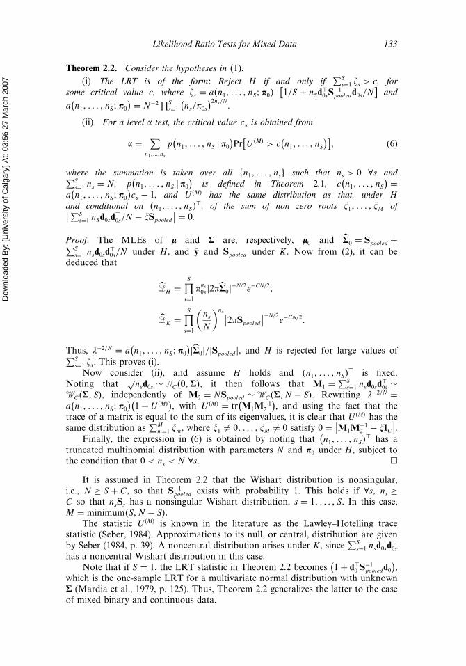
Theorem 2.2. Consider the hypotheses in �1�.(i) The LRT is of the form: Reject H if and only if

∑Ss=1 �s > c, for

some critical value c, where �s = a�n1� � � � � nS� �0�[1/S + nSd

�0sS

−1pooledd0s/N

]and

a(n1� � � � � nS� �0

) = N−2∏Ss=1

(ns/�0s

)2ns/N .(ii) For a level test, the critical value c is obtained from

= ∑n1�����ns

p(n1� � � � � nS � �0

)Pr[U�M� > c

(n1� � � � � nS

)]� (6)

where the summation is taken over all �n1� � � � � ns� such that ns > 0 ∀s and∑Ss=1 ns = N , p

(n1� � � � � nS � �0

)is defined in Theorem 2.1, c

(n1� � � � � nS

) =a(n1� � � � � nS� �0

)c − 1, and U�M� has the same distribution as that, under H

and conditional on �n1� � � � � nS��, of the sum of non zero roots �1� � � � � �M of∣∣∑S

s=1 nSd0sd�0s/N − �Spooled

∣∣ = 0.

Proof. The MLEs of � and � are, respectively, �0 and �0 = Spooled +∑Ss=1 nsd0sd

�0s/N under H , and y and Spooled under K. Now from (2), it can be

deduced that

�H =S∏

s=1

�ns0s �2��0�−N/2e−CN/2�

�K =S∏

s=1

(ns

N

)ns ∣∣2�Spooled

∣∣−N/2e−CN/2�

Thus, �−2/N = a(n1� � � � � nS� �0

)��0�/�Spooled�, and H is rejected for large values of∑Ss=1 �s. This proves (i).Now consider (ii), and assume H holds and �n1� � � � � nS�

� is fixed.Noting that

√nsd0s ∼ �C�0���, it then follows that M1 =

∑Ss=1 nsd0sd

�0s ∼

�C��� S�, independently of M2 = NSpooled ∼ �C��� N − S�. Rewriting �−2/N =a(n1� � � � � nS� �0

)(1+ U�M�

), with U�M� = tr

(M1M

−12

), and using the fact that the

trace of a matrix is equal to the sum of its eigenvalues, it is clear that U�M� has thesame distribution as

∑Mm=1 �m, where �1 �= 0� � � � � �M �= 0 satisfy 0 = ∣∣M1M

−12 − �IC

∣∣.Finally, the expression in (6) is obtained by noting that

(n1� � � � � nS�

� has atruncated multinomial distribution with parameters N and �0 under H , subject tothe condition that 0 < ns < N ∀s. �

It is assumed in Theorem 2.2 that the Wishart distribution is nonsingular,i.e., N ≥ S + C, so that S−1

pooled exists with probability 1. This holds if ∀s, ns ≥C so that nsSs has a nonsingular Wishart distribution, s = 1� � � � � S. In this case,M = minimum�S� N − S�.

The statistic U�M� is known in the literature as the Lawley–Hotelling tracestatistic (Seber, 1984). Approximations to its null, or central, distribution are givenby Seber (1984, p. 39). A noncentral distribution arises under K, since

∑Ss=1 nsd0sd

�0s

has a noncentral Wishart distribution in this case.Note that if S = 1, the LRT statistic in Theorem 2.2 becomes

(1+ d�0 S

−1pooledd0

),

which is the one-sample LRT for a multivariate normal distribution with unknown� (Mardia et al., 1979, p. 125). Thus, Theorem 2.2 generalizes the latter to the caseof mixed binary and continuous data.

Dow

nloa

ded

By: [

Uni

vers

ity o

f Cal

gary

] At:

03:5

6 27

Mar

ch 2

007

134 de Leon

Observe that while the LRTs in Theorems 2.1 and 2.2 are derived from theunconditional likelihood function, they are assessed conditionally on the totalcounts across states for the binary data. This conditioning is computationallyconvenient because it reduces the burden of getting a critical value or p-valueto summing tail probabilities over a set of counts for a contingency table. Animportant consideration in the unknown covariance case (i.e., Theorem 2.2) isthe distribution of U�M�. Bilodeau and Brenner (1999) provides an exact andcomputationally efficient way of evaluating this distribution, which we use in thesimulations in Sec. 4.

We establish the consistency and unbiasedness of the LRTs in Theorems 2.1and 2.2 in the next section.

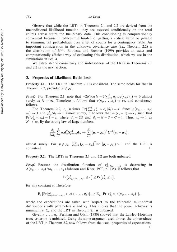
3. Properties of Likelihood Ratio Tests

Property 3.1. The LRT in Theorem 2.1 is consistent. The same holds for that inTheorem 2.2, provided � �= �0.

Proof. For Theorem 2.1, note that −2N logN − 2∑S

s=1 ns log(�0s/ns

)→ 0 almostsurely as N → . Therefore it follows that c�n1� � � � � nS� → , and consistencyfollows.

For Theorem 2.2, c satisfies Pr(∑S

s=1 �s > c � �0) = . Since a

(n1� � � � � nS�

�0

)→ 1 and �2d2/d2 → 1 almost surely, it follows that d2�c − 1� → c0 such thatPr��2d1 ≤ c0� = 1− , where d1 = CS and d2 = N − S − C + 1. Thus, c → 1 asN → . By the strong law of large numbers,

d2

Nd1

S∑s=1

nsd�0sS

−1pooledd0s →

S∑s=1

(�s − �0s

)��−1

(�s − �0s

)�

almost surely. For � �= �0,∑S

s=1

(�s − �0s

)��−1

(�s − �0s

)> 0 and the LRT is

consistent. �

Property 3.2. The LRTs in Theorems 2.1 and 2.2 are both unbiased.

Proof. Because the distribution function of �2d1���n1�����ns� is decreasing in��n1� � � � � nS� ∀n1� � � � � nS (Johnson and Kotz, 1970, p. 135), it follows that

Pr[�2d1���n1�����nS� ≤ c

] ≤ Pr[�2d1 ≤ c

]�

for any constant c. Therefore,

E�

{Pr[�2d1���n1�����nS� > c

(n1� � � � � nS

)]} ≥ E�0

{Pr[�2d1 > c

(n1� � � � � nS

)]}�

where the expectations are taken with respect to the truncated multinomialdistributions with parameters � and �0. This implies that the power achieves itsminimum at �0, and the LRT in Theorem 2.1 is unbiased.

Given n1� � � � � nS , Perlman and Olkin (1980) showed that the Lawley–Hotellingtrace criterion is unbiased. Using the same argument used above, the unbiasednessof the LRT in Theorem 2.2 now follows from the usual properties of expectations.

�

Dow

nloa

ded

By: [

Uni

vers

ity o

f Cal

gary

] At:

03:5

6 27

Mar

ch 2

007

Likelihood Ratio Tests for Mixed Data 135

The above results include that for the case C = 1 and S = 2, details of whichare found in de Leon and Carrière (2000).

4. Simulation Study

To evaluate the performance of the LRT in terms of its nominal level and power,we conducted a series of simulation experiments using mixed data generated fromthe GLOM with C = 2 and S = 4. This model corresponds to the case of twocontinuous variables y� = �Y1� Y2� and the binary vector x� = �X1� � � � � X4�. Theparameter is then �� = (

��� ��), where �� = (�1� � � � � �4�, �

� = (��1 � �

�2

)with ��

s =(1s� 2s

)the sth �s = 1� � � � � 4� state mean vector of y. Data were simulated from

this GLOM with sample sizes N = 50� 100, and 160, and this was repeated 10,000times. The hypothesized value �0 under the null hypothesis H in (1) was specifiedas ��

0 = �0�25� 0�25� 0�25� 0�25�, �01 = �02 = �03 = �04 = �0� 0��, and the covariancematrix was taken to be

� =(

1 0�5

0�5 1

)�

To assess the level and power of the LRT, the following five cases wereconsidered:

(0) no differences between hypothesized and true populations;(a) there is difference between hypothesized and true populations only with respect

to binary vector x;(b) there is difference between hypothesized and true populations only with respect

to continuous vector y;(c) hypothesized and true populations are different with respect to both variable

types.

Note that (0) corresponds to the case where H is true. For (a), we consideredthe cases (a1) �� = �0�2� 0�3� 0�25� 0�25�, and (a2) �� = �0�2� 0�3� 0�1� 0�4�. For (b),we have (b1) ��

1 = �0�2� 0�2�, �2 = �3 = �4 = �0� 0��; (b2) ��1 = �0�2� 0�2�, ��

2 =�−0�2�−0�2�, �3 = �4 = �0� 0��; (b3) ��

1 = �0�2� 0�2�, ��2 = �−0�2�−0�2�, ��

3 =�0�4� 0�4�, ��

4 = �0� 0�; and (b4) ��1 = �0�2� 0�2�, ��

2 = �−0�2�−0�2�, ��3 = �0�4� 0�4�,

��4 = �−0�4�−0�4��. For (c), we have (c1) �� = �0�2� 0�3� 0�25� 0�25� and ��

1 =�0�2� 0�2� ��

2 = �−0�2�−0�2�, �3 = �4 = �0� 0��; (c2) �� = �0�2� 0�3� 0�25� 0�25� and��1 = �0�2� 0�2�� ��

2 = �−0�2�−0�2�� ��3 = �0�4� 0�4�� ��

4 = �−0�4�−0�4��; (c3) �� =�0�2� 0�3� 0�1� 0�4�, and ��

1 = �0�2� 0�2�, ��2 = �−0�2�−0�2�, �3 = �4 = �0� 0��; and

(c4) �� = �0�2� 0�3� 0�1� 0�4� and ��

1 = �0�2� 0�2�, ��2 = �−0�2�−0�2�, ��

3 = �0�4� 0�4�,��4 = �−0�4�−0�4��.

Tables 1 and 2 display the simulation results, the former for the case of knowncovariance matrix and the latter for that of unknown covariance matrix. Criticalvalues were obtained by the bisection method in both cases, and the power functionin (5) was used to evaluate the theoretical power of the LRT in the case of knowncovariance matrix. Observe from Table 1 that the empirical power values are quiteclose to their theoretical values, as expected.

Dow

nloa

ded

By: [

Uni

vers

ity o

f Cal

gary

] At:

03:5

6 27

Mar

ch 2

007

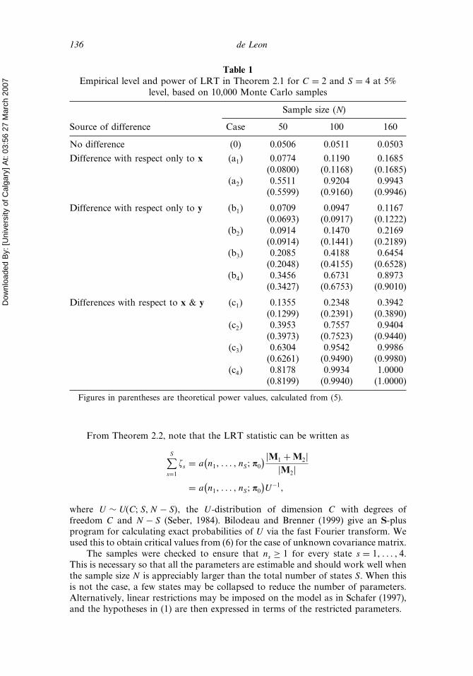
136 de Leon

Table 1Empirical level and power of LRT in Theorem 2.1 for C = 2 and S = 4 at 5%

level, based on 10,000 Monte Carlo samples

Sample size �N�

Source of difference Case 50 100 160

No difference (0) 0.0506 0.0511 0.0503

Difference with respect only to x (a1) 0.0774 0.1190 0.1685(0.0800) (0.1168) (0.1685)

(a2) 0.5511 0.9204 0.9943(0.5599) (0.9160) (0.9946)

Difference with respect only to y (b1) 0.0709 0.0947 0.1167(0.0693) (0.0917) (0.1222)

(b2) 0.0914 0.1470 0.2169(0.0914) (0.1441) (0.2189)

(b3) 0.2085 0.4188 0.6454(0.2048) (0.4155) (0.6528)

(b4) 0.3456 0.6731 0.8973(0.3427) (0.6753) (0.9010)

Differences with respect to x & y (c1) 0.1355 0.2348 0.3942(0.1299) (0.2391) (0.3890)

(c2) 0.3953 0.7557 0.9404(0.3973) (0.7523) (0.9440)

(c3) 0.6304 0.9542 0.9986(0.6261) (0.9490) (0.9980)

(c4) 0.8178 0.9934 1.0000(0.8199) (0.9940) (1.0000)

Figures in parentheses are theoretical power values, calculated from (5).

From Theorem 2.2, note that the LRT statistic can be written as

S∑s=1

�s = a(n1� � � � � nS� �0

) �M1 +M2��M2�

= a(n1� � � � � nS� �0

)U−1�

where U ∼ U�C� S� N − S�, the U -distribution of dimension C with degrees offreedom C and N − S (Seber, 1984). Bilodeau and Brenner (1999) give an S-plusprogram for calculating exact probabilities of U via the fast Fourier transform. Weused this to obtain critical values from (6) for the case of unknown covariance matrix.

The samples were checked to ensure that ns ≥ 1 for every state s = 1� � � � � 4.This is necessary so that all the parameters are estimable and should work well whenthe sample size N is appreciably larger than the total number of states S. When thisis not the case, a few states may be collapsed to reduce the number of parameters.Alternatively, linear restrictions may be imposed on the model as in Schafer (1997),and the hypotheses in (1) are then expressed in terms of the restricted parameters.

Dow

nloa

ded

By: [

Uni

vers

ity o

f Cal

gary

] At:

03:5

6 27

Mar

ch 2

007

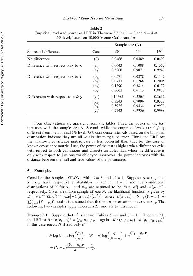
Likelihood Ratio Tests for Mixed Data 137

Table 2Empirical level and power of LRT in Theorem 2.2 for C = 2 and S = 4 at

5% level, based on 10,000 Monte Carlo samples

Sample size (N )

Source of difference Case 50 100 160

No difference (0) 0.0488 0.0489 0.0493

Difference with respect only to x (a1) 0.0643 0.1088 0.1552(a2) 0.5288 0.9071 0.9943

Difference with respect only to y (b1) 0.0571 0.0878 0.1142(b2) 0.0717 0.1268 0.2005(b3) 0.1590 0.3814 0.6172(b4) 0.2662 0.6113 0.8832

Differences with respect to x & y (c1) 0.10865 0.2205 0.3652(c2) 0.3243 0.7096 0.9323(c3) 0.5935 0.9434 0.9979(c4) 0.7743 0.9936 0.9999

Four observations are apparent from the tables. First, the power of the testincreases with the sample size N . Second, while the empirical levels are slightlydifferent from the nominal 5% level, 95% confidence intervals based on the binomialdistribution indicate they are all within the margin of error. Third, the LRT forthe unknown covariance matrix case is less powerful than that for the case ofknown covariance matrix. Last, the power of the test is higher when differences existwith respect to both continuous and discrete variables than when the difference isonly with respect to just one variable type; moreover, the power increases with thedistance between the null and true values of the parameters.

5. Examples

Consider the simplest GLOM with S = 2 and C = 1. Suppose x = x�1� andx = x�2� have respective probabilities p and q = 1− p, and the conditionaldistributions of Y for x�1� and x�2� are assumed to be �

(1� �

2)and �

(2� �

2),

respectively. Given a random sample of size N , the likelihood function is given by� = pnqN−n�2��2�−N/2 exp

[−Q(1� 2

)/(2�2

)], where Q

(1� 2

) =∑ni=1

(Yi − 1

)2 +∑Ni=n+1

(Yi − 2

)2, and it is assumed that the first n observations have x = x�1�. The

following two examples apply Theorems 2.1 and 2.2 to this model.

Example 5.1. Suppose that �2 is known. Taking S = 2 and C = 1 in Theorem 2.1,the LRT of H � �p� 1� 2�

� = (p0� 01� 02

)�against K �

(p� 1� 2

)� �= (p0� 01� 02

)�in this case rejects H if and only if

−N logN − n log(p0

n

)− �N − n� log

(q0

N − n

)+ n

��Y1 − 01�2

�2

+ �N − n���Y2 − 02�

2

�2>

c 2�

Dow

nloa

ded

By: [

Uni

vers

ity o

f Cal

gary

] At:

03:5

6 27

Mar

ch 2

007

138 de Leon

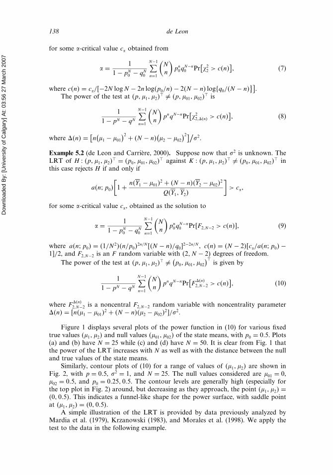
for some -critical value c obtained from

= 11− pN

0 − qN0

N−1∑n=1

(Nn

)pn0q

N−n0 Pr

[�22 > c�n�

]� (7)

where c�n� = c /�−2N logN − 2n log�p0/n�− 2�N − n� log�q0/�N − n�}].

The power of the test at �p� 1� 2�� �= �p� 01� 02�

� is

11− pN − qN

N−1∑n=1

(Nn

)pnqN−nPr

[�22���n� > c�n�

]� (8)

where ��n� = [n(1 − 01

)2 + �N − n�(2 − 02

)2]/�2.

Example 5.2 (de Leon and Carrière, 2000). Suppose now that �2 is unknown. TheLRT of H � �p� 1� 2�

� = �p0� 01� 02�� against K � �p� 1� 2�

� �= �p0� 01� 02�� in

this case rejects H if and only if

a�n� p0�

[1+ n��Y1 − 01�

2 + �N − n���Y2 − 02�2

Q��Y1��Y2�]> c �

for some -critical value c , obtained as the solution to

= 11− pN

0 − qN0

N−1∑n=1

(Nn

)pn0q

N−n0 Pr�F2�N−2 > c�n��� (9)

where a�n� p0� = �1/N 2��n/p0�2n/N ��N − n�/q0�

2−2n/N , c�n� = �N − 2��c /a�n� p0�−1�/2, and F2�N−2 is an F random variable with �2� N − 2� degrees of freedom.

The power of the test at �p� 1� 2�� �= (

p0� 01� 02

)�is given by

11− pN − qN

N−1∑n=1

(Nn

)pnqN−nPr

[F

��n�2�N−2 > c�n�

]� (10)

where F��n�2�N−2 is a noncentral F2�N−2 random variable with noncentrality parameter

��n� = �n�1 − 01�2 + �N − n��2 − 02�

2�/�2.

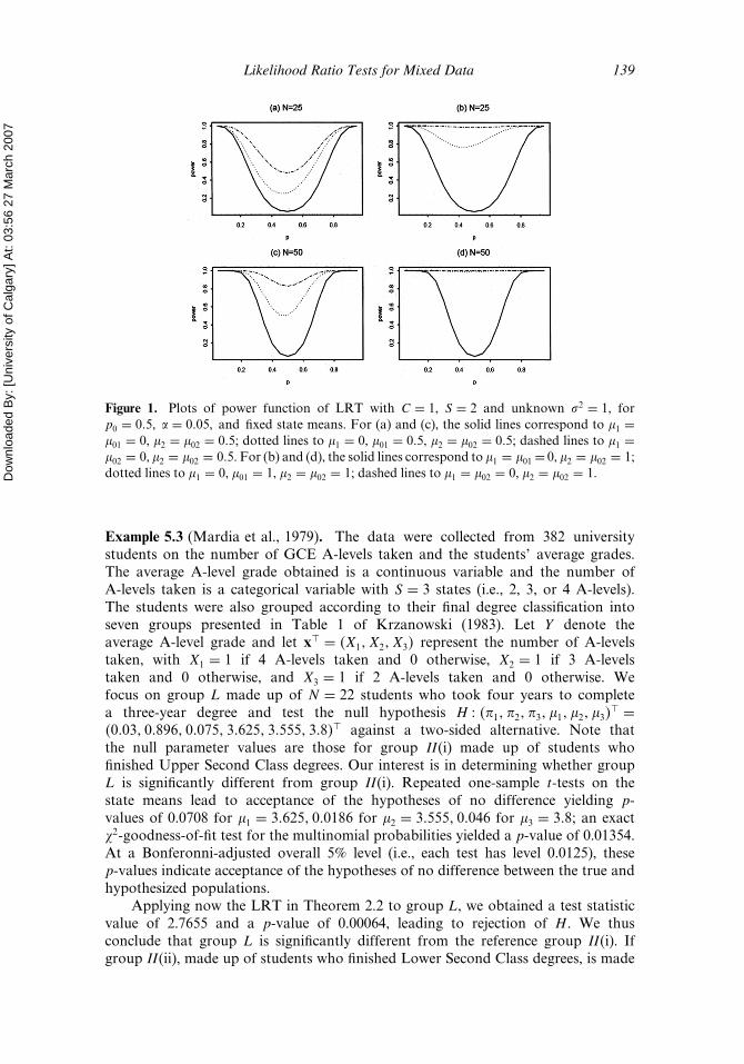
Figure 1 displays several plots of the power function in (10) for various fixedtrue values �1� 2� and null values �01� 02� of the state means, with p0 = 0�5. Plots(a) and (b) have N = 25 while (c) and (d) have N = 50. It is clear from Fig. 1 thatthe power of the LRT increases with N as well as with the distance between the nulland true values of the state means.

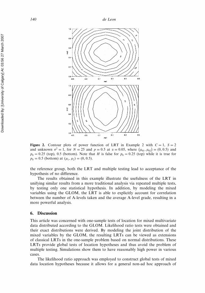
Similarly, contour plots of (10) for a range of values of �1� 2� are shown inFig. 2, with p = 0�5, �2 = 1, and N = 25. The null values considered are 01 = 0,02 = 0�5, and p0 = 0�25� 0�5. The contour levels are generally high (especially forthe top plot in Fig. 2) around, but decreasing as they approach, the point �1� 2� =�0� 0�5�. This indicates a funnel-like shape for the power surface, with saddle pointat �1� 2� = �0� 0�5�.

A simple illustration of the LRT is provided by data previously analyzed byMardia et al. (1979), Krzanowski (1983), and Morales et al. (1998). We apply thetest to the data in the following example.

Dow

nloa

ded

By: [

Uni

vers

ity o

f Cal

gary

] At:

03:5

6 27

Mar

ch 2

007

Likelihood Ratio Tests for Mixed Data 139

Figure 1. Plots of power function of LRT with C = 1, S = 2 and unknown �2 = 1, forp0 = 0�5, = 0�05, and fixed state means. For (a) and (c), the solid lines correspond to 1 =01 = 0, 2 = 02 = 0�5; dotted lines to 1 = 0, 01 = 0�5, 2 = 02 = 0�5; dashed lines to 1 =02 = 0, 2 = 02 = 0�5. For (b) and (d), the solid lines correspond to 1 = 01 = 0, 2 = 02 = 1;dotted lines to 1 = 0, 01 = 1, 2 = 02 = 1; dashed lines to 1 = 02 = 0, 2 = 02 = 1.

Example 5.3 (Mardia et al., 1979). The data were collected from 382 universitystudents on the number of GCE A-levels taken and the students’ average grades.The average A-level grade obtained is a continuous variable and the number ofA-levels taken is a categorical variable with S = 3 states (i.e., 2, 3, or 4 A-levels).The students were also grouped according to their final degree classification intoseven groups presented in Table 1 of Krzanowski (1983). Let Y denote theaverage A-level grade and let x� = �X1� X2� X3� represent the number of A-levelstaken, with X1 = 1 if 4 A-levels taken and 0 otherwise, X2 = 1 if 3 A-levelstaken and 0 otherwise, and X3 = 1 if 2 A-levels taken and 0 otherwise. Wefocus on group L made up of N = 22 students who took four years to completea three-year degree and test the null hypothesis H � ��1� �2� �3� 1� 2� 3�

� =�0�03� 0�896� 0�075� 3�625� 3�555� 3�8�� against a two-sided alternative. Note thatthe null parameter values are those for group II(i) made up of students whofinished Upper Second Class degrees. Our interest is in determining whether groupL is significantly different from group II(i). Repeated one-sample t-tests on thestate means lead to acceptance of the hypotheses of no difference yielding p-values of 0.0708 for 1 = 3�625� 0�0186 for 2 = 3�555� 0�046 for 3 = 3�8; an exact�2-goodness-of-fit test for the multinomial probabilities yielded a p-value of 0.01354.At a Bonferonni-adjusted overall 5% level (i.e., each test has level 0.0125), thesep-values indicate acceptance of the hypotheses of no difference between the true andhypothesized populations.

Applying now the LRT in Theorem 2.2 to group L, we obtained a test statisticvalue of 2.7655 and a p-value of 0.00064, leading to rejection of H . We thusconclude that group L is significantly different from the reference group II(i). Ifgroup II(ii), made up of students who finished Lower Second Class degrees, is made

Dow

nloa

ded

By: [

Uni

vers

ity o

f Cal

gary

] At:

03:5

6 27

Mar

ch 2

007

140 de Leon

Figure 2. Contour plots of power function of LRT in Example 2 with C = 1, S = 2and unknown �2 = 1, for N = 25 and p = 0�5 at = 0�05, where

(01� 02

) = �0� 0�5� andp0 = 0�25 (top), 0.5 (bottom). Note that H is false for p0 = 0�25 (top) while it is true forp0 = 0�5 (bottom) at �1� 2� = �0� 0�5�.

the reference group, both the LRT and multiple testing lead to acceptance of thehypothesis of no difference.

The results obtained in this example illustrate the usefulness of the LRT inunifying similar results from a more traditional analysis via repeated multiple tests,by testing only one statistical hypothesis. In addition, by modeling the mixedvariables using the GLOM, the LRT is able to explicitly account for correlationbetween the number of A-levels taken and the average A-level grade, resulting in amore powerful analysis.

6. Discussion

This article was concerned with one-sample tests of location for mixed multivariatedata distributed according to the GLOM. Likelihood ratio tests were obtained andtheir exact distributions were derived. By modeling the joint distribution of themixed variables by the GLOM, the resulting LRTs can be viewed as extensionsof classical LRTs in the one-sample problem based on normal distributions. TheseLRTs provide global tests of location hypotheses and thus avoid the problem ofmultiple testing. Simulations show them to have reasonably high power in variouscases.

The likelihood ratio approach was employed to construct global tests of mixeddata location hypotheses because it allows for a general non-ad hoc approach of

Dow

nloa

ded

By: [

Uni

vers

ity o

f Cal

gary

] At:

03:5

6 27

Mar

ch 2

007

Likelihood Ratio Tests for Mixed Data 141

simultaneously accounting for both the discrete (i.e., multinomial) and continuousvariables in the data. The approach parallels that of Afifi and Elashoff (1969) andis an alternative to the dissimilarity-based tests proposed by Morales et al. (1998).These tests, it should be noted, are all asymptotic, unlike the exact LRTs derived inthe article.

The test statistics are similar to their continuous case counterparts and aresimple and easy to calculate. In addition, critical values of the tests can bereadily obtained by conventional methods. Alternatively, one may resort to usingasymptotic distributions to carry out the tests. Another alternative is suggestedby the decomposition of the likelihood function into discrete and continuouscomponents. An overall test can then be constructed by adding, say, a �2-goodness-of-fit test statistic to a suitably scaled version of Hotelling’s T 2 statistic. The sizeand power of such a test should be explored vis-a-vis those of the LRTs proposedin the article.

Acknowledgments

The author was supported by a Studentship Award from the Alberta HeritageFoundation for Medical Research (AHFMR) and by a grant from the NaturalSciences and Engineering Research Council of Canada. He is grateful to YongtaoZhu for computational assistance and to the referee for very helpful commentswhich greatly improved the form and content of the article.

References

Afifi, A. A., Elashoff, R. M. (1969). Multivariate two sample tests with dichotomous andcontinuous variables. I. The location model. Ann. Math. Stat. 40:290–298.

Bilodeau, M., Brenner, D. (1999). Theory of Multivariate Statistics. New York: Wiley & Sons.Catalano, P. J. (1997). Bivariate modeling of clustered continuous and ordered categorical

outcomes. Statist. Med. 16:883–900.de Leon, A. R., Carrière, K. C. (2000). On the one-sample location hypothesis for mixed

bivariate data. Commun. Statist. Theor. Meth. 29(11):2573–2581.Fitzmaurice, G. M., Laird, N. M. (1995). Regression models for a bivariate discrete and

continuous outcome with clustering. J. Amer. Statist. Assoc. 90:845–852.Johnson, N. L., Kotz, S. (1970). Continuous Univariate Distributions. Vol. 2. New York:

Houghton Mifflin.Krzanowski, W. J. (1983). Distance between populations using mixed continuous and

categorical variables. Biometrika 70:235–243.Little, R. J., Rubin, D. B. (1987). Statistical Analysis with Missing Data. New York: Wiley &

Sons.Liu, C., Rubin, D. B. (1998). Ellipsoidally symmetric extensions of the general location

model for mixed categorical and continuous data. Biometrika 85:673–688.Mardia, K. V., Kent, J. T., Bibby, J. M. (1979).Multivariate Analysis. London: Academic Press.Morales, D., Pardo, L., Zografos, K. (1998). Informational distances and related statistics in

mixed continuous and categorical variables. J. Statist. Plann. Infer. 75:47–63.Olkin, I., Tate, R. F. (1961). Multivariate correlation models with mixed discrete and

continuous variables. Ann. Math. Stat. 32:448–465 (correction in 36:343–344).Perlman, M. D., Olkin, I. (1980). Unbiasedness of invariant tests for MANOVA and other

multivariate problems. Ann. Statist 8:1326–1341.Schafer, J. L. (1997). Analysis of Incomplete Multivariate Data. New York: Chapman & Hall.Seber, G. A. F. (1984). Multivariate Observations. New York: Wiley & Sons.