On Multiparameter Quantum SL and Quantum Skew-symmetric Matrices

Alexis Dite

Doctor of Philosophy

University of Edinburgh

2006

Abstract Since its beginning in the early 1980s the subject of Quantum Groups has expan-

ded to include many areas of mathematics. We will be concerned with studying

two particular quantized coordinate rings from an algebraic perspective.

The first quantized coordinate ring under investigation is Multiparameter

Quantum SL. In Chapter 2, inspired by an observation in a paper by Dipper

and Donkin, we tackle the problem of defining a quantum analogue of SL in

the Multiparameter Quantum Matrices setting when the quantum determinant is

not central. We construct a candidate for this algebra in a natural way using the

process of Noncommutative Dehomogenisation. We go on to show that the object

defined has many appropriate properties for such an analogue and observe that

our new algebra can also be obtained via a process known as twisting. Finally we

see what our definition means in the particular case of Dipper-Donkin Quantum

Matrices and also look at the Standard Quantum Matrices case.

In Chapter 3 we move on to our other object of study, Quantum Skew-

symmetric Matrices. This was defined, along with the concept of q-Pfaffians, in

a paper by Strickland in 1996. We show that this algebra is an iterated skew

polynomial ring, and we are able to read off many results by applying the ma-

chinery detailed in a book by Brown and Goodearl. We go on to show that a

q-Laplace expansion of q-Pfaffians holds and that the highest-length q-Pfaffian is

central. Finally we show that a factor of Quantum Skew-symmetric Matrices is

isomorphic to Cq(2, n).

Quantum Skew-symmetric Matrices are also mentioned in a 1996 paper by

Noumi. In Chapter 4 we recall his definition of the algebra and of q-Pfaffians.

These definitions are different to those of Strickland. We show that, when q is not

a root of unity, these contrasting definitions are in fact the same. Using Noumi's

definition we show that another Laplace-type expansion, the natural q-analogue

of a classical result, holds for q-Pfaffians.

In the final chapter we investigate the commutation relations between the

q-Pfaffians. In proving the centrality of the highest-length q-Pfaffian in Chapter

3 we determine some specific commutation relations; these are used in Chapter 5

to establish more general results. We observe that the set of q-Pfaffians has the

structure of a partially ordered set and show that our relations are well-behaved

with respect to this structure.

Acknowledgements

My greatest debt of gratitude goes, of course, to my supervisor Tom Lenagan, His

temperament was ideally suited to my own. Thanks also go to Matyas Domokos

for his clear insight and for hosting an enjoyable and fruitful stay in Budapest. I

would also like to thank Ken Goodearl for some useful comments. The generosity

of the Liegrits programme and Freddy Van Oystaeyen enabled me to complete

this thesis in the wonderful city of Antwerp. On a personal note I would like

to thank the Glasgow Algebraists for treating me as one of their own, my office

mates in 4620, and most of all Marcie.

Contents

Chapter 1 Introduction 3

1.1 Coalgebras, Bialgebras, and Hopf Algebras .............3

1.2 Skew Polynomial Rings ........................6

1.3 Quantum Groups ...........................8

1.4 Noncommutative Properties .....................10

1.5 Skew-symmetric Matrices and Pfaffians ...............11

Chapter 2 Multiparameter Quantum SL 14

2.1 Noncommutative Dehomogenisation .................15

2.2 Skew-Laurent Extensions and Hopf Algebras ............16

2.3 Constructing a Candidate for 0,(SL) .............. 18

2.4 Properties of our O,(SL) ..................... 23

2.5 A Link with 0,\,p(GL) ........................ 28

2.6 An Unexpected Isomorphism .....................32

2.7 Twisting ................................36

2.8 The Dipper Donkin Case .......................37

2.9 The Standard Quantum Matrices Case ...............38

Chapter 3 Quantum Skew-symmetric Matrices 40

3.1 Definitions and Preliminaries .....................41

3.2 Oq(Skn) is an Iterated Skew Polynomial Ring ...........44

3.3 A Torus Action ............................51

3.4 A Laplace Expansion of Pfq .....................53

3.5 Pfq is Central .............................58

3.6 A Link with Gq (2, ii) .........................68

Chapter 4 Oq(Skn), A Different Perspective 71

4.1 Noumi's Approach ..........................71

4.2 The Equivalence of Strickland and Noumi .............73

4.3 Another Laplace-type Expansion ..................86

1

Chapter 5 Further Properties of (9q(Skn ) 91

5.1 Commutation Relations .......................91

5.2 Reflection in the Anti-diagonal ....................108

5.3 A Partial Ordering ..........................114

Bibliography 121

Index 124

01,

Chapter 1

Introduction

The main objects of study in this thesis are two algebras that can be thought of

as quantized coordinate rings. The purpose of this first chapter is to introduce

the terminology that we will use to describe and investigate them. We claim no

originality for any of the material in this chapter, it is all well known. Indeed we

also claim no originality for the presentation, most of the material having been

already presented in perfect clarity in [4] - a book which we take as our main

source of inspiration. Our sole purpose is to fix our notation and gather together

the language and results that will frame the rest of the thesis.

Throughout this thesis, if not explicitly stated, K will denote a fixed base field

and tensor products, ®, will be over K. All rings and algebras will be assumed

to contain a unit element.

1.1 Coalgebras, Bialgebras, and Hopf Algebras

Many of the algebras that we will encounter will possess, or will be proved to

possess, the structure of either a coalgebra, bialgebra, or a Hopf algebra. In this

section we will give definitions of these, and related, concepts - material that can

all be found in, for example, [1], [4], [8], and [22].

Definition 1.1.1. A coalgebra (C, A, e) is a K-vector space C, together with

K-linear maps A : C - C ® C, called the comultiplication, and c : C —p K,

called the counit, such that the following diagrams commute:

C

C ®C C®C C®C id C®C

~'o i ~d Oi~d Zido,

C®C®C C

Remark 1.1.2. If we think of an algebra as being a K-vector space A, together

with K-linear maps i : A ® A -f A, ij : K -* A representing multiplication

(a ® b ab) and unit (a -* a 1) respectively, then the commutative diagrams

in the previous definition are exactly those that one obtains by "dualizing" the

commutative diagrams involving i and 'q that represent the usual algebra axioms

for A.

Notation 1.1.3. We will follow the Sweedler notation convention and write

A(c) = E c1 0c2

for an element c E C.

Definition 1.1.4. An element g in a coalgebra C is said to be grouplike if A(g) =

g ® g and e(g) = 1.

Definition 1.1.5. A map f : C -p D between coalgebras C and D is said to be

a coalgebra morphism if it is a linear map such that AD o f = (f ® f) o Ac and

ED ° f = EC .

Definition 1.1.6. A subspace I of a coalgebra C is a coideal if A(I) c C®I+

10 and €(I) = 0. It is easy to see that C/I is then a coalgebra with the induced

comultiplication and counit.

A coalgebra that also has the structure of an algebra is called a bialgebra if the

two structures are well-behaved with respect to each other, that is:

Definition 1.1.7. A bialgebra (B, , r, A, e) is a K-vector space B, together with

K-linear maps ,u, 'ij, A, e such that (B, p, ,q) is an algebra, (B, A, e) is a coalgebra

and the following equivalent conditions hold:

A and c are algebra morphisms, or

p and i are coalgebra morphisms.

Definition 1.1.8. A map f : B - D between bialgebras B and D is a bialgebra

morphism if it is both an algebra morphism and a coalgebra morphism.

Definition 1.1.9. A subspace I of a bialgebra B is a biideal if it is both a coideal

with respect to the coalgebra structure of B and an ideal with respect to the algebra

structure. In this case it follows that B/I is a bialgebra.

4

Definition 1.1.10. A Hopf algebra (H, 1u, i, A, €, S) is a K-vector space H with

K-linear maps ,.t, 'ri, A, e making (H, u, r, A, e) into a bialgebra, together with a

K-linear map S: H - H called the antipode, such that, in Sweedler notation,

= €(h) 'H = h1S(h2)

for all h E H. Let us define the convolution product *, of two maps f,g E

Horn jc(H, H) to be

(f*g)(h) = f(hi)g(h2)

for h E H. Then the previous condition on S may be written as,

S*id=Tioe=id*S.

We will often say "H is a Hopf algebra" instead of "(H, p, Ti A, e, S) is a Hopf

algebra" taking the various maps as implied.

The following well-known lemma is useful when working with Hopf algebras:

Lemma 1.1.11. The antipode, S, of a Hopf algebra, H, is an algebra anti-

morphism, that is, S(ab) = S(b)S(a) for all a, b E H.

Definition 1.1.12. A map f : H -k C between Hopf algebras H and G is a

Hopf algebra morphism if it is a bialgebra morphism such that f o Si-i = SG o f.

In Chapter 2 we will have cause to show that certain maps between Hopf algebras

are Hopf algebra morphisms. To reduce the amount of work needed to be done

in these instances we will call upon a result that we have found only in [8]. Being

less well-known we provide a specific reference:

Proposition 1.1.13. [8, Proposition 4.2.5] Let f : H -f C be a map between

Hopf algebras H and C. Suppose f is a bialgebra morphism. Then it follows that

f is a Hopf algebra morphism.

Finally the definitions we have seen for coideals and biideals have their appropriate

Hopf-analogue:

Definition 1.1.14. A subspace I of a Hopf algebra H is a Hopf ideal if it is a

biideal such that 5(I) c I. In this case H/I is a Hopf algebra.

5

Dual to the notion of modules of algebras is the concept of comodules of coalgeb-

ras:

Definition 1.1.15. Let C be a coalgebra. A right C-comodule is a K-vector

space V with a linear map p : V -* V ® C, called the coaction, such that the

following diagrams commute:

V

~p

Nc

V ®C V®C id V®C

V®C®C V

Just as when we talk about the "representation theory" of an algebra we are re-

ferring to its modules, when we talk of the "corepresentation theory" of an object

with a coalgebra structure we refer to its comodules.

To end this section we define a structure that we will encounter in Chapter 3.

Suppose we have an algebra H and an H-module, A. If H is in fact a bialgebra

and A is in fact an algebra, then it is desirable that these extra structures interact

in a "nice" way, that is:

Definition 1.1.16. Let H be a bialgebra and A an algebra. We say that A is a

left H-module algebra if A is a left H-module such that

h(ab) = Eh(hl(a))(h2(b)) for h E H and a, b E A; and

h(1A)==e(h).1A.

1.2 Skew Polynomial Rings

In this section we give another set of definitions and results that will form part of

the fundamental language that we use throughout this thesis. All this material

and much more can be found in [17].

Let R be a ring and let o be an automorphism of R.

Definition 1.2.1. An additive map 6 : r -) R is called a a-derivation (more

precisely a left a-derivation) on R if 6(rs) = a(r)8(s) + 6(r)s for all r, s C R.

Let 6 be a a-derivation on R. Then we can form the skew polynomial ring R[x; a, 6]

where xr = a(r)x+6(r) for r E R. This can be constructed explicitly as a subring

6

of a certain ring of endomorphisms, but we are only concerned with the properties

that it possesses:

Definition 1.2.2. Let R be a ring, let a be an automorphism of R, and let 8 be

a a-derivation on R. Then T = R[x; a, 8] means

T is a free left R-module with basis {x' : n E N}.

x'r = a(r)x + 8(r) for all r e R.

Remark 1.2.3. The above definition would work just as well if a were only an

endomorphism of R, but we will always require a to be an automorphism. Also

we note here, that if R is also a K-algebra then we will always assume that a is

a K-algebra automorphism and 6 is K-linear.

When working with skew polynomial rings we will always write elements with

left-hand coefficients, that is for f E R we will write it in the form

f = rx + r_ix 1 + rx + r0

where rn,. . . , r0 E R and we will say that f is of degree n (assuming r 0).

Definition 1.2.4. If our 6 = 0 then we may localize R[x; a] at the set consisting

of the powers of x and form the skew-Laurent ring R[x,x';cr].

We now give two key results concerning skew polynomial rings.

Lemma 1.2.5. If R is a domain then the skew polynomial ring R[x; C7,6] is a

domain.

Theorem 1.2.6. If R is noetherian then so is R[x; a, 6].

Many of the algebras that we encounter are not only skew polynomial rings but

are in fact iterated skew polynomial rings over K. We now give a precise definition

of what this means.

Definition 1.2.7. We say A is an iterated skew polynomial ring over R and

write

A = R[xi;ai,81][x2;a2,82] .. {x;a,8]

ifR[xi; al , 81 ] is askew polynomial ring and for each Ai R[xi;ai ,81] ...

Ai is a skew polynomial ring over A_1 (i = 2,. .. , n).

Remark 1.2.8. Of course a quick induction extends the previous two results to

the case of iterated skew polynomial rings.

7

1.3 Quantum Groups

The area of Quantum Groups that we will be interested in is that of "quantized

coordinate rings" viewed from an algebraic perspective. By a quantized coordin-

ate ring we mean a noncommutative "deformation" of the coordinate ring of an

algebraic group or a related algebraic variety. The simplest example is that of

the quantum plane. The classical coordinate ring of the plane, (9(K2), is just

K[x, y], polynomials in two commuting variables. For a nonzero element q E K<

we define the quantized coordinate ring of the plane (or quantum plane for short)

to be

Qq(K 2) = K(x,y : xy = qyx).

We do not just allow any noncommutative version of a classical object but usually

restrict ourselves to ones which retain certain "nice" properties from the classical

case. With the quantum plane it is not hard to see that it is an iterated skew

polynomial ring over K and so is a noetherian domain, properties that hold for

the classical coordinate ring of the plane. Also setting q = 1 brings us back to

the classical case - another feature of desirable quantum analogues.

The standard example of a quantized coordinate ring that we will keep in mind

throughout this thesis is that of Quantum Matrices [32], [33]. In the classical

case the coordinate ring of n x n matrices is just the polynomial ring generated

by the n2 coordinate functions, tij say, that pick out the ij-th entry of a matrix.

The standard quantum version of this is defined below. Throughout what follows

q will be a nonzero element of our base field K and we shall write 4 := (q - q').

Definition 1.3.1. Let n be a positive integer. The coordinate ring of quantum

n x n matrices, (9q(Mn) is the K-algebra generated by the n2 indeterminates

{t : i, j = 1, ..., n}, subject to the following relations:

tjjtji = qtt,

tjjtkj = qtk t,

tjltkj = tkjtjl,

tjjtkl = tkltjj + 4t1tkJ 7

for 1 < j < k < n and 1 < j < 1 < n. The language we have established

in the previous two sections now comes into play. It is known (see for example

[4, Theorem 1.2.7]) that (9q(Mn) is an iterated skew polynomial algebra over K

and hence a noetherian domain. It also possesses a bialgebra structure with the

natural comultiplication and counit:

(tjk) =

tij ® tjk

e(tk) = Jik -

There is a distinguished element of this algebra known as the quantum determin-

ant, denoted by detq ,

detq = (—q)1 tl, (l)t2, (2) tn,7r (n) 7rES

where 1(7), is the length of the permutation n. Note that if we set q = 1 then we

have the classical definition of the determinant. By [33, Theorem 4.6.1] we know

that detq is in the centre of Oq(Mn). So analogously to the classical case we may

define Oq(GLri ) and (9q(SLn) as follows:

Oq(GLn) := Oq(Mn) [detq 1 ] and Oq(SLn) Oq(Mn)

(detq - 1)

Now it can be worked out that detq is a grouplike element of Oq(Mn), that is

A(detq) = detq ® detq and e(detq ) = 1, and so the bialgebra structure of Oq (M)

induces bialgebra structures on Oq(GLn) and Oq(SLn). Furthermore from [33,

Theorem 5.3.21 we know that (9q(GLn) and Oq(SLn) are Hopf algebras with

antipode given by

S(t) = (_q)[ 31 ]deç'

where Z= {1, ..., n} \ {i}. We will now explain what we mean by [j I i ]. Just

as in [161, for index sets I, J with Ill = we use the notation [IIJ] to denote

the quantum determinant of Oq(Mj, j ) the quantum matrix subalgebra of (9q (Mn)

generated by the elements tij with i E I, j E J. We will call [Il J] the quantum

minor with rows I and columns J. This leads us on to the definition of our

final example of a quantized coordinate ring, namely the quantum grassmanian

[23]. Firstly we note that Definition 1.3.1 can be naturally extended to enable us

to define quantum m x n matrices, Oq(Mmn). The quantum in x n grassmanian,

Cq(m, n) is then defined to be the subalgebra of Oq(Mmn) generated by the m in

quantum minors of Oq(Mmn).

Before leaving this section we should point out that the original objects to be

defined in Quantum Groups were not quantized coordinate rings but rather quant-

ized enveloping algebras. These are noncommutative deformations of the universal

enveloping algebra of a Lie algebra. We will not discuss these here, although we

shall encounter an example of such an object in Chapter 3.

9

1.4 Noncommutative Properties

This section is a mixed bag of definitions. For completeness we collect here the

definitions of various "noncommutative properties" that we refer to later in the

thesis. We begin by presenting the definition of Gelfand-Kirillov dimension, a

useful tool when dealing with noncommutative algebras. The standard reference

for all things Gelfand-Kirillov is [26].

Definition 1.4.1. Let A be a finitely generated K-algebra. Let V be a finite

dimensional K-subspace of A containing 'A such that V generates A as an algebra

and let V denote the linear span of all products of at most n elements of V. The

Gelfand-Kirillov dimension of A is defined to be:

log dimK (V'2)

GKdim(A) = lim sup log

Remark 1.4.2. In /26, Lemma 1.11 it is shown that the above definition is inde-

pendent of the choice of V.

We will use GKdim more than once to show that a map under consideration is

an isomorphism. To do this we will make use of the following two results which

we record here:

Lemma 1.4.3. [26, Lemma 3.1] If B is a subalgebra or a homomorphic image of

a K-algebra A, then GKdim(B) < GKdim(A).

Proposition 1.4.4. [26, Proposition 3.15] Let I be an ideal of a K-algebra A,

and assume that I contains a right regular element or a left regular element of A.

Then

CKdim(A/I) +1 < GKdim(A).

Next we deal with various homological properties that are considered "nice" for

a noncommutative ring to satisfy. They can be viewed as the appropriate non-

commutative analogues of homological conditions used in commutative algebra.

Requiring a noncommutative noetherian ring to have finite injective or global

dimensions turns out to be too lenient to be useful and so an extra condition is

imposed, see for example [28], [35], [36]. Our sources for the presentation of these

definitions are the survey paper [6] and [4, Appendix 1.15].

Let R be a noetherian ring.

Definition 1.4.5. The grade of a finitely generated R-module M is defined to be

j(M) := inf{i > 0: Ext(M, R) L 01.

10

Definition 1.4.6. Note that for a left (right) R-module M and for i > 0,

Ext(M, R) is a right (left) R-module via the right (left) action on H. We say

that a noetherian ring R satisfies the Auslander condition if j(N) ~: i for all fi-

nitely generated R-submodules N c Ext(M, R) for every finitely generated right

or left H-module M and for all i > 0.

Definition 1.4.7. A noetherian ring R is Auslander-Gorenstein if it satisfies the

Auslander condition and has finite right and left injective dimension.

Definition 1.4.8. A noetherian ring R is Auslander-regular if it is Auslander-

Corenstein and has finite global dimension.

Definition 1.4.9. An algebra A is said to be Cohen-Macaulay if

j(M) + GKdim(M) = GKdim(A) <oo

for every nonzero finitely generated A-module M.

Finally, we briefly record the definition of the noncommutative Nullstellensatz

given in [4]:

Definition 1.4.10. [4, Definition 11.7.14] Let A be a noetherian K-algebra. We

say that A satisfies the Nullstellensatz over K provided A is a Jacobson ring and

that the endomorphism ring of every irreducible A-module is algebraic over K.

1.5 Skew-symmetric Matrices and Pfaffians

In the final three chapters of this thesis we will be concerned with investigating

the quantum analogue of the coordinate ring of skew-symmetric matrices. In this

section we recall the basic setup of the classical situation and recall some known

identities.

An n x n matrix over K, A = (a1 ) say, is skew-symmetric if At = —A. In

that case we have aji = —aij for i < j and in particular aii = 0, that is A has

zeros on its main diagonal. So we can see that a skew-symmetric matrix A is

completely determined by its upper-triangular elements, and we shall write A as

a12 aln

A= a_

The coordinate ring of skew-symmetric matrices, (.9(Sk), is therefore commut-

ing polynomials in the n(n - 1)/2 upper-triangular coordinate functions. This

11

coordinate ring is a representation for the general linear group GL". If we think

of our aii as the coordinate functions on a general skew-symmetric matrix and

arrange them in our matrix A, then the action of GL on (9(Sk) is given by

X(A) = XAX 1, for X E CL.

We see (9(Sk) in this context in [2]. Crucial to the understanding of Q(Sk)

in [2] are the Pfaffians of skew-symmetric matrices - a concept related to the

determinant. If n is odd then the determinant of a skew-symmetric matrix is

zero. So from now on we restrict ourselves to the cases where n is even:

det ( a12) = a

21

a12 a13 a14\

det ( a23 a24) = (a

12a34 - a13a24 + a14a23 )2. a34

We see that the determinant in these two examples is the square of a polynomial

in the entries of the matrix. In 1849 Cayley proved that this held in general, and

the polynomial in question is the Pfaffian of the skew-symmetric matrix (for a

historical overview of Pfaffians we refer the reader to [25]). We will now give a

precise definition of a Pfaffian and then some Pfaffian identities. The following

material comes from [13, Appendix D], [24], and [19].

Let A be a n x n skew-symmetric matrix with n = 2m.

Definition 1.5.1. Let Fn be the subset of Sn consisting of elements a such that

a(2i —1) <a(2i) for Z' = 1,...,m and o- ( 2i —1) < (2i + 1) for = 1,...,m —1.

Then the Pfaffian of A, which we denote Pf(A), is

Pf(A) (-1)1 a(1)(2) a_)) crEF

where 1(a) is the length of the permutation a.

Since all the a13 commute we have the following equivalent definition:

Definition 1.5.2. Let 1l, := {a E Si-, : a(2i - 1) <a(2i) for i = 1, ..., m}. Then

Pf(A) =

Since ci 1 = — a13 for i <j we can relax the restrictions on the permutations still

further and so we also have the equivalent definition:

12

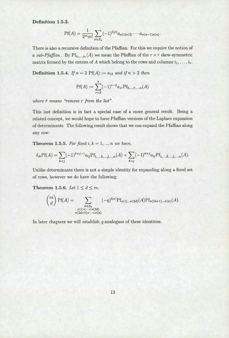
Definition 1.5.3.

Pf(A) = 1

(-1)1 aa(l)(2) a_i)). 2mm!

o.Es fl

There is also a recursive definition of the Pfaffian. For this we require the notion of

a sub-Pfaffian. By Pf, jr (A) we mean the Pfaffian of the r x r skew-symmetric

matrix formed by the entries of A which belong to the rows and columns i1,. , i,..

Definition 1.5.4. If n = 2 Pf(A) := a12 and if n> 2 then

Pf(A) := (_1)T_2airPf2 n(A)

where means "remove r from the list".

This last definition is in fact a special case of a more general result. Being a

related concept, we would hope to have Pfaffian versions of the Laplace expansion

of determinants. The following result shows that we can expand the Pfaffian along

any row:

Theorem 1.5.5. For fixed i, k = 1, ..., n we have,

8kPf(A) = (_1)3_1ajjPf1 k.... 3.... (A) + (_1)aiPf1k....3 k<j k>j

Unlike determinants there is not a simple identity for expanding along a fixed set

of rows, however we do have the following:

Theorem 1.5.6. Let 1 <d < m.

(n)

Pf(A) = aESn

o(1)<...<a(2d)

In later chapters we will establish q-analogues of these identities.

13

Chapter 2

Multiparameter Quantum SL

Let K be a field. Let A be a nonzero element of K with A —1, and let p be

a multiplicatively antisymmetric n x ri matrix over K. In this chapter we are

concerned with the multiparameter deformation of the coordinate ring of ri x n

matrices O,(M) [3]. This is the K-algebra generated by n2 indeterminates

{x : i,j = 1, ...,n}, subject to the following relations:

XjmXjj = PljPjmXjjXlm + (A - 1)p1iximx1j for 1 > i, m > j (2.0.1)

Xlrn Xij = APiipjmxijxim for I > i, m < j (2.0.2)

Xlm Xij = PjmXtjXlm for m > j (2.0.3)

where i,j,1,m=1,...,n.

The algebra O,(M) is an N-graded noetherian domain [4, Theorem 1.2.7]. It

is also a bialgebra with the natural comultiplication and counit:

A(xik ) = Xii ® Xik

= öik.

The Quantum Determinant is [4, Definitions 1.2.3] the element

DA,p = i H (Pir(i),7r(j)) Xl,(l)X2,(2) ... Xn,(n). irS, 1<i<j<ri

ir(i)>ir(j)

It is known (e.g. [15, Section 1.3]) that DA, p is a normal element of OA,p(M),

satisfying the following relations, for all i, j,

DA,pxii = A3 (fipjlpli) xjDAp.

In the literature OA,(SL) is only defined when D N , p is central. When it is merely

normal, factoring out (DA, p - 1) from 0,\, p(Mn ) leaves us with the coordinate ring

14

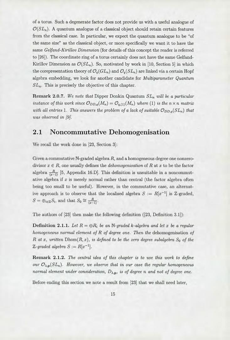
of a torus. Such a degenerate factor does not provide us with a useful analogue of

(9(SL). A quantum analogue of a classical object should retain certain features

from the classical case. In particular, we expect the quantum analogue to be "of

the same size" as the classical object, or more specifically we want it to have the

same Celfand-Kirillov Dimension (for details of this concept the reader is referred

to [26]). The coordinate ring of a torus certainly does not have the same Gelfand-

Kirillov Dimension as O(SL). So, motivated by work in [10, Section 5] in which

the corepresentation theory of Oq(GL) and (9q(SLn) are linked via a certain Hopf

algebra embedding, we look for another candidate for Multiparameter Quantum

SL. This is precisely the objective of this chapter.

Remark 2.0.7. We note that Dipper Donkin Quantum SL will be a particular

instance of this work since ODD,q(Mn) = (9q ,( 1) (Mn) where (1) is then x n matrix

with all entries 1. This answers the problem of a lack of suitable ODD,q(SLn) that was observed in /9J.

2.1 Noncommutative Dehomogenisation

We recall the work done in [23, Section 3]:

Given a commutative N-graded algebra R, and a homogeneous degree one nonzero-

divisor x E R, one usually defines the dehomogenisation of R at x to be the factor

algebra -y [5, Appendix 16.D]. This definition is unsuitable in a noncommut-

ative algebra if x is merely normal rather than central (the factor algebra often

being too small to be useful). However, in the commutative case, an alternat-

ive approach is to observe that the localised algebra S := R[x 1 ] is Z-graded,

S =(E)iEZSi,and that So

The authors of [23] then make the following definition ([23, Definition 3.1]):

Definition 2.1.1. Let R = be an N-graded k-algebra and let x be a regular

homogeneous normal element of R of degree one. Then the dehomogenisation of

R at x, written Dhom(R, x), is defined to be the zero degree subalgebra So of the

ZZ-graded algebra S:= R[x'].

Remark 2.1.2. The central idea of this chapter is to use this work to define

our 0A, p (SL). However, we observe that in our case the regular homogeneous

normal element under consideration, D,\ , is of degree n and not of degree one.

Before ending this section we note a result from [23] that we shall need later,

15

Lemma 2.1.3. Let R and x be as above. Then R is a domain if and only

if Dhom(R, x) is a domain. Moreover, if R is noetherian then Dhom(R, x) is

noet he vi an.

2.2 Skew-Laurent Extensions and Hopf Algebras

The following results concerning the creation of new Hopf algebras and bialgebras

from existing ones will be necessary in the next section:

Lemma 2.2.1. Let H be a Hopf algebra and let or be a Hopf algebra automorphism

of H. Then the skew-Laurent extension H[t, t 1; a] is also a Hopf algebra.

Proof. We extend the algebra morphisms A and e, and the algebra antimorphism

S on H, (the comultiplication, counit and antipode maps of H, respectively), to

maps on H[t, t'; a] in the obvious way; that is, for E H[t, t'; a],

( h()t) := [ht ® hti]

h(')t'):=

(iiti) :=

It is now a matter of checking whether these definitions give H[t, t 1; a] a Hopf

algebra structure. The fact that H[t, t'; a] is a coalgebra follows immediately

from the coalgebra properties of H. To show that H[t, t 1; a] is also a bialgebra

is not as straightforward. We must show that our extended A and € are algebra

morphisms of H[t, t 1; a].

Let

u= ht', v = e H[t,t 1 ; a].

We show that our extended A is an algebra morphism. Now,

(uv) = A ((hti)(g(i) ti)

)

= A (E htigti)

= A (

hai(g)ti+i),

16

by definition of H[t, t 1; a]. Applying our extended definition of tx to the RHS

gives,

= ® ii O)Oli

= ® ® t) i,.? h()o(g(i))

= ® ij

by definition of A on H. Since H is a Hopf algebra, A is an algebra morphism

on H, hence,

A(uv) = ® t)]. ij

Now a is, in particular, a coalgebra morphism on H, so it follows that,

A(uv) = [A (0) ) (a ® a) (A (g())) ® t)ij

where the above deductions have used the definitions of A, H[t, t'; a], and simple

rearranging. So we have shown that A is an algebra morphism. The proof that

e is an algebra morphism is similar.

Finally we must show that our extended S is an antipode for H[t, t'; a]. It

17

suffices to show that S * id = id * S = r€. We show that id * S = ije, the other

case being similar. Now by definition of the convolution product,

(id *5) (

h(i)ti) = [(hti)S(hti)] .

Applying our extended definition of S we deduce that,

(id *5) (

h(Oti) = [(hti)(t—iS(h))]

= [E 1 2 (hS(h))] i h()

=

where the last equality holds since S is an antipode for H. Finally by our extended

definition of e we have,

(id * S) (

h(i)ti) = € (

h(i)ti),

and so we are done. 701

Lemma 2.2.2. Let R be a bialgebra and let a be a bialgebra automorphism of R.

Then the skew-Laurent extension R[t, t'; a] and the skew extension R[t; a] are

bialge bras.

Proof. The proof is similar to the proof of the previous result.

2.3 Constructing a Candidate for (9,p(SLn)

We noted in a previous section that was of degree n, thus preventing us from

using directly the Noncommutative Dehomogenisation of [23] to define O (SL).

Instead we make the following construction. For the sake of clarity let us set

A := At this point we must suppose there exist

E K and q = (qjj) E M(K) such that A = jf and Pu = q (2.3.1)

with q multiplicatively antisymmetric. Define a map

a : A by a(xu) ( U qjkqki) xij. (2.3.2)

extending in the natural way.

I1

Lemma 2.3.1. The map a is a bialgebra auiomorphism.

Proof. To prove that a is a well-defined algebra morphism it suffices to show that

it respects the relations (2.0.1), (2.0.2), and (2.0.3). We deal with (2.0.1), the

other cases being similar. Let I > i, m > j. Then,

a(xjmxjj) = a(xim)a(xjj) n

= m+j-1-i I

H mkk1ikki) XlmXij

k=1

(k=1

n m+j-1-i

H mkktikki) (PliPjmXijXlm + (A - 1)p1j x jm xj j ),

where the last equality holds by (2.0.1). Thus,

n a(xjmxjj) = ,1m+j-1-i

(fT qmkqklqjkqki)plipjmxijxlm

k=1

+ (A -

By definition of a it follows that,

a(x mx jj ) = PiiPjmU(Xij)0(Xim) - (A - 1)pija(xjm)a(xjj),

and since a is, by construction K-linear, we have,

cr(ximxjj) = a(plipjmxijxlin + ( A 1)piiximXtj).

Hence a is indeed an algebra morphism. Our next task is to show that a is a

coalgebra morphism. Now,

= (3_%

(k=" ikki) x)

= 3i (ri 1 ikki) e(x)

= ui_i (n qjkqki ) .

Since 8jj is nonzero only when i = j, we may deduce that

= i_ (n)

qikqki 6ij. .

19

But qikqki = 1 by definition of q, so,

= 6ij

=

Also,

(a (D a)(A(x)) =a (x) ® a(xi)

= ( (

,r-i 11 ') X1) ®

(qjkqkr Xrj)

= i (

rkkrkiik) (Xi r ® Xrj),

and since qrkqkr = 1,

(a (9 a)(A(xj)) = (

, fl

ri E jr ® Xrj

k=1

=

" 1

-i (

qjkqki

) (x)

= (i_i (ri ikki) x)

=

So a is also a coalgebra morphism. Hence or is a bialgebra morphism.

Finally we note that a is clearly an automorphism of A.

So by Lemma 2.2.2 we may form the bialgebra A, [u; a]. We note that the auto-

morphism a has been constructed so that u'2 commutes like DA,. Now A is

N-graded so clearly if we let u have degree one then A, [u; a] is also N-graded.

Let B := A[u; a]/(u - DA P). We are, in essence, adjoining an n th root of

to A. Now, by definition, u is a grouplike element of An [U; a]. It is also the

case that DA,p is grouplike (this follows from the argument on page 890 of [3]

concerning the invariance of comultiplication under so-called twists and the well

known result that the standard quantum determinant is grouplike [32, (1.11)]).

So it follows that (u" - DA,p) is a homogeneous biideal of A [u; a]. Hence B is a

N-graded bialgebra.

Now, by definition of a, the element u is normal in A, [u; a] and hence u (or

20

more precisely the element u + ( n - we shall henceforth abuse notation

and refer to this element as u) is normal in B.

We now go on to show that u is regular in B. However, before we do, we re-

quire the following result which shows us that u and D),,p commute.

Lemma 2.3.2. a(DA,P) =

Proof. Since a is an algebra morphism it follows that,

a(DA,p) fl (pi,j) (fta(Xr(r))) irES 1<i<j<n r=1

ir(i) >ir(j)

by the definition of a we have,

a(DA,p) fi () (ft(r)_r(Üq(r)kqkr)xr(r)) irES 1<i<j<n r=1 k=1

7r(i) >i(j)

which can be written equivalently as,

a(DA)

( II (_P(i)U))) q(r),kqkr) (r="lH Xr,n(r)

irES 1<i<jn \k=1 r=1 I 7T(i)>7r(j)

Now 7(r) =En r since 7V E S is a bijection. So (ir(r)—r) = 1. Also, iv

being a bijection, together with the fact that q is multiplicatively antisymmetric,

allows us to deduce that fl1(H1 q(r),kqkr) = 1. Hence,

(DA,p) = fi ( pj,j) (n a Xrn(r))

i-cS 1<jn r 1 7T(i) >ir(j)

=

U

Lemma 2.3.3. The element u is regular in B.

Proof. We first require the fact that elements of B may be expressed as polyno-

mials in u over An of degree less than or equal to n - 1.

21

Let f C A[u;a]. Then f = > i0 fu for some m E N and fi E A. Sup-

pose m > n. Then,

f =fu

rn-i = frnUm_Th(UTh - D),p) + (fm-n + fmDA,p)flm_n +

iom-n

since u and DA,p commute by Lemma 2.3.2. So modulo (m - DA,p) the element f

is equivalent to a polynomial of degree ni - 1. Hence, by induction, we are done.

Now suppose there exists g E B such that ug = 0 in B. By the above we

may write g = >I say. So we have, by the definition of B,

ug E (u n - DA,p)

(: giui - D,p)

E (u - DA,p).

By consideration of degree in u it follows that,

= b(u - DA,p) for some b e A.

Comparing coefficients of u0 yields that bDA, = 0, and so, since A is a domain,

we have that b = 0. It follows that g = 0. Hence u is not a left zero divisor.

Similarly u is not a right zero divisor, and so we are done. El

We have just shown that the normal element u is regular in B. We also have, by

definition, that u is of degree one. So u is such that we may use the method of

Noncommutative Dehomegenisation to consider the algebra C :=Dhom(B, u). It

is this algebra, C, which we propose as a candidate for OA,p(SLn).

Definition 2.3.4. Given that K is such that (.3.1) holds,

(0,\,p

OA,p(Mn)[u; U 01

(SL) := Dhom -

).

The rest of the chapter is concerned with proving results concerning the properties

of C.

22

2.4 Properties of our 0A,(SL)

We note that, as an algebra, C is generated by {xu-' : i,j =1, ...,n}. This can easily be seen by examining the definition of B and Dhom(B, u). Let cij = xu 1 . Then, using relations (2.0.1), (2.0.2), and (2.0.3), together with (2.3.2), it may be calculated that, for i, j, 1, m = 1, ..., n,

clmcij = i+m—j-1 (ñ kiikmkk1) PliPjmCijClm

+ (A - 1)p 1 (H cimclj,

for I > i, m > j, (2.4.1)

clmcij APiiPjm+m_3_1 (n qkjqikqmkqkl) CjjClm,

for 1 > i, m <j, (2.4.2)

ClmClj pjmm_ U J ( qkjqmk) CijClm,

for m > j. (2.4.3)

Now by Lemma 2.2.2 since An is a bialgebra and - is a biideal it follows that B[u'] = A[u,u1;a]/(u - is a bialgebra (we note that B[u 1 ] = A[u, tr 1 ; cr]/(u' - DA P) by [17, Exercises 91 and 9L]). Now, as in Lemma 2.2.1, we may extend A and e as defined on A to A, [u, tt'; a] and hence to B[u'J. So, in particular, we have,

A(c j) = A(xu')

=XU ® XkjU '

= Cik ® Ckj,

and,

= e(xu 1 )

=

= 6ij.

Hence C is a subbialgebra of B[u'] (it is sufficient to check closure on the gen-erators since A and e are algebra morphisms on B[u 1]).

23

Proposition 2.4.1. C is a Hopf algebra.

Proof. We have just shown above that C is a subbialgebra of B[r']. We noted

that

B[f 1] = A[u,u';o]/(u - DA,p),

and so the bialgebra structure of B[u'] comes from the bialgebra structure of

A. Likewise, we will show that C is a sub-Hopf-algebra of B[?r1], the Hopf al-

gebra structure of which comes from the Hopf algebra structure of 0,\,p(GL) =

A [D]. This can be seen more clearly upon inspection of the following com-

mutative diagram

Anc An [u; o] An[U;C] B (u' -

u a] B[u'] (u—DA) A(

A, [u,

An [D > (A[D])

f1p [u, u1;

(An[D])E,u';I A 1 C

(u'—D,)

A little thought yields that ço is in fact an isomorphism (with u being sent to

D under ,o). So we have that,

(A ID—ll'\ [u,u';a]

B[u'] nL Api)

- - DA,p)

Now in [3, Theorem 3] the authors prove that A[D] is a Hopf algebra with

antipode S: A[D] - A[D] defined by

i—i j-1

= (fJ(-p772)) (fl (-p8))[ 3 7Th=1 s=1

S(D,) =DA p

We are using here the terminology of quantum minors, [ 3 ], as in [16].

That is, i = {1, ..., n} \ {i} and [I I J] denotes, in our case, the multipara-

meter quantum determinant of the matrix subalgebra generated by the elements

Xrs with r E I and s C J, where I and J are index sets of the same cardinal-

ity. More extensive definitions of these terms are given in [3, Theorem 31 but

with [3 I i ] denoted by U. Since A[D] is a Hopf algebra it follows by 1p

Lemma 2.2.1 that (A[D]) [u, u 1; a] is a Hopf algebra. It is not hard to see

that (u" - DA,p) is a Hopf ideal of (A. [D—')) [u, u 1 ; a], and so it follows that

(A[D]) [u, u 1; a]/(u - DA p), and hence B[u 1], is a Hopf algebra. Keeping

24

in mind that "u behaves like a nthroot of it is easy to see that the antipode

for B[u], coming from S, is S: B[u1] -> B[u] defined by

i-i j-1

S(x) = ([J( — pim))(JJ( — p3j))[ i I i 1u, M=1 3=1

S(u) =

S(tr') =

Claim: S induces an antipode on C.

Proof: The bialgebra C is a subbialgebra of B[u 1 ] so it suffices to show that

C is closed under S. Since S is an algebra antiendomorphism it suffices to check

this on the generators of C. Now,

S(c) = S(xu)

S(u 1)S(x)

=

By definition of S and i ], we may write,

S(x) = 77ii

for some qij, r E K, where the above sum runs over all bijections

Hence,

S(c) = Ujj

We note that in each term of the above sum we have a product of exactly n - 1

Xjm '5. It is clear from the definition of A, [u, u; cr] that we may "move along

powers of u past the Xlm" to obtain,

S(c)= 77ij E Tr

7r

r0i

for some i E K. But this is just

S(c) = 77ij 7r fJ(iccr,ir (r)).

It ri

Hence C is a Hopf algebra. FM

25

Proposition 2.4.2. C is Noetherian.

Proof. Since Q,(M) is Noetherian, so is O,p(Mn)[u; u]/(u - DA,p). Hence C

is Noetherian by [23, Corollary 3.3]. 1-1

Lemma 2.4.3. An/An D,,,p is a domain.

Proof. This is [20, Example 3]. LI

Proposition 2.4.4. C is a domain.

Proof. Now by Lemma 2.1.3 it suffices to prove that B is a domain. Now, as seen

earlier, any element of B = An [U; ]/(u"—D,) can be thought of as a polynomial

in u over An of degree less than or equal to n 1. Let us write 6 = for

convenience. Let 0 f, g E A[u; cr]/(u - 6). Say,

f=fu, g=gflJ

where f, g3 e A and are not all zero. Suppose

f9=0 in A[u;0-]/(u-6).

We will show that this leads to a contradiction. Now we have,

( j=0

fui) gj) E (u' - 6)

that is,

f1ugu = E (uTh

i,j=O i,j=O

By consideration of degree in u, we have,

fa(g)u r3u(u i,j=O s=O

for some r8 E An. Since u and 6 commute (by Lemma 2.3.2),

n—i n-2

fi(g)ui+i = ( r 3u fl+S - r58u3 ),

i,j=O s=O

which can be rewritten as,

2n-2 2n-2 n-2

fjot(g) Um = r—um + (_rm6)um.

m=O i+j=m m=n rn=O

26

Comparing coefficients we have,

:i: fu(g) = 0 i+j=m- 1

E f ai(g ) fa(g)6, s=0,...,n-2. i+j8 i+j=S+fl

We may as well assume there exist i, j such that 6 t fi and 6 t g (in A) since

otherwise, using the fact that A is a domain, we could replace the problem with

f'ai(g')=::O

i+j=n- 1

f/ai(g) = - ff(9)8 s=0,...,n-2 i+j=s i+j=3+n

where deg(ffl < deg(f) or deg(g) < deg(g). Iterating this process we would

eventually come to a stage where we have an fit) and a g(t) not divisible by J.

Let k be minimal such that 6 t fk and let 1 be minimal such that 6 { gj. Suppose

6 1 fko(gj). Then since A,/A,,6 is a domain by Lemma 2.4.3, 61 fk or 6 I So by choice of k we must have 6 1 o(gj). Now by Lemma 2.3.2 we have that

8 = 0(6) I o(gj); that is, ak(gj ) = yak(6) for some y E A. Since ci is an

automorphism it follows that 8 1 gj, which contradicts our choice of 1. Hence

6 fak(g1). (2.4.4)

This will be the main tool to show that our supposition that B is not a domain

leads to a contradiction.

We will require that k + I - n > 0. Let us prove this now. First, suppose

k+1 <n-2. Now,fors_—k+l, (B) says,

6 I foa°(gk+1) + ... + f_1ak_l(g11) + fuk(g1) + fk+lak+1( \911) + ... + fk+1a 1 (go).

By definition of k and 1, along with the fact that ci is an automorphism with

cr(S) = 8, we know that 61 fi for i = 0,...,k— land 6 I crt(gj) for = 0,...,1— 1

and for any t. So we can deduce that 8 I fko(g1) which contradicts (2.4.4). Hence

k + 1 > n - 2. Now let us suppose that k + 1 = n - 1. By (A),

f cTk(gj ) = - fcr"(g). (2.4.5) i+j=n-1 st (i,j)O(k,1)

By choice of k and 1,

j I fi Vi<k=rm—1—1, (2.4.6)

6g Vj<I=n—1—k. (2.4.7)

27

Consider fo'(g) such that i +j = n - 1 with i k. First suppose i < k. Then

6 1 fji(g) by (2.4.6). Next, suppose i> k. Then j = n - 1 - i <n - 1 - k =

and so by (2.4.7) we have 8 1 gj. Hence 6 = o(6) I a(g3 ), and so 6 I fa(g).

Thus by (2.4.5) we have 6 I fak(gj) which contradicts (2.4.4). So we may deduce

that k + 1 > n.

We are now in a position to consider fo(g) such that i + j = k + I - n > 0.

Supposeik. Thenj=k+l—n—i _<k+1—n—k=1—n. But ln-1,

so j < —1 which is clearly false. Hence i < k. Suppose j ~: 1. Then, as above,

it follows that i < —1 which again is clearly false. Hence j < 1. So by choice of

k and 1, we have, 8 I fi and 6 I g3 . It follows that 62 I fa'(g). For s = k + I - n

(B) says that,

ft?(g3 ) = - fcr(g j)6. i+j=k+1-n i+j=k+1

Now, we have just shown that 82 I fu(g) Vi + j = k + 1 - n, so we can deduce

that 62 I fo(g)6.

i+j=k+1

Since A is a domain we have that

6 1 foa°(gk+j) + ... + f iak_l(gj+i) + fak(g1) + fk+lak+l(gj_l) + ... + f1k+i(g)

Since we know that 6 I fVi < k and 6 I gVj < I it follows that 8 I f ko(g1 ) which

is a contradiction by (2.4.4). Hence f = 0 or g = 0, and so B is a domain. fl

2.5 A Link with O,\,(GL)

Now in [10, Section 5] a link between the corepresentation theory of (9q(SL(n))

and Oq(GL(n)) is given by the authors showing that one can find a Hopf algebra

embedding,

Oq (GL (n)) .' Oq (SL (n))[z,z']

It is a further argument in favour of our candidate for 0,\,p(SL) that we can find

a similar relationship between it and 0,\,p(GL) (which, as alluded to earlier, is

a Hopf algebra by [3, Theorem 3]). Reflecting the fact that in our case we have

normal rather than central D X,p the embedding is not into Laurent polynomials

over OA,p(SL), rather it is into Skew-Laurent polynomials over OA,p(SL).

Now by [23, Lemma 3.21,

C[z,z 1;] B[u'],

where a is the automorphism on C induced by the automorphism of B[ir1 ] given

by b -* ubu 1 for b E B. One can see that,

: C C is given by cj _i(flqjqj)cjj. (2.5.1)

That is,

=

Lemma 2.5.1. : C -i C is a Hopf algebra morphism.

Proof. By [8, Proposition 4.2.5] it suffices to show that & is a bialgebra morphism.

Now we know that a -f A, is a bialgebra morphism. One may check that

this can be extended to a bialgebra morphism a' : A,, [u, u 1; a] -f A,2 [u, u 1; a]

by setting cr'(xu) := u(x)u-' for x E A. Now by Lemma 2.3.2 a(DA,) = so

- DA, p) = - a(DA,) = - D.

Hence a' factors to give a bialgebra morphism a" on

B[u 1] = A[u,u';a]/(u - DA,p).

On C, we observe that a" = &, and so we are done. LI

We are now in a position to form the Hopf algebra C[z, z; ] by Lemma 2.2.1.

Henceforth we shall abuse notation and write a for &. Before establishing the

Hopf algebra embedding we require the following lemma,

Lemma 2.5.2.

irES, 1<i<j<ri r=1 7r(i)>7r(j)

Proof. Now, by definition of the c,

(—P(),(j)) fi ar_i (Cr(r)) II rES, 1<i<j<n r=1

7r(i)>7r(j)

= II (P(i),(j))

7rES, 1<i<j<ri r=1 ir(i)>ir(j)

29

and by definition of or this gives,

II H ar(c)

7rES i<i<j<n r=i ir(i) >7r(j)

fl (j) fi ar_i (Xr(r))U1 irES 1<i<j<n r=1

7(i)>7r(j)

Since, for x E A, xu 1 u-'a(x), we can see that,

ar_i (Xr,(r))U' = (ft Xr(r)) irtm, (2.5.2)

and using this to rewrite the previous equation gives,

H (Pi),j)) H ari(c)

irES i<i<j<ri r=i 7r(i)>7r(j)

= (P(i),

(

'r(j))ftXr(r)) 7TESn 1<i<g5ri r=1

-0)>-O)

=1.

Proposition 2.5.3. There exists a Hopf algebra embedding,

O, (GL) -+ O(SL,) [z, z; a].

Proof. Define an algebra morphism

A,,A'P [D-'] -* C[z, z'; a] by x cz and D F-* z

We first show that this is indeed a well-defined algebra morphism. That is, we

show ' respects the relations of A [D]. Firstly,

= H (P(i),(j)) ftXr,(r) 7rESn i<i<j<ri r=i

ir(i) >ir(j)

= H (p(),()) (ftCr, (r)Z). 71ES,-. 1<i<j<n r=1

ir(i) >7r(j)

30

Similar to (2.5.2) in the proof of the previous lemma, because of the definition of

C[z, z 1 ; a], we can "move the z's to the right" in the above product, giving us,

= H (— ,i) (H Ur_l(Cr(r)))ZTh

TES 1<i<j<n r=1 ir(i)>r(j)

= Zn,

where the last equality holds by the previous lemma. We now show that respects

relation (2.0.1). For 1 > i, m > j, we have

/(Xim Xjj P1iPjmXijX1m — (A - 1)piiXim Xij)

= CImZCijZ - PliPjmCijZCimZ - (.\ - 1)PIiCimZCI3Z

(CIMU(cij) —piipjmcija(cim) - ( l)plicima(Clj))Z2

=0

where the last equality is a consequence of relation (2.4.1). Similarly 0 respects

relations (2.0.2) and (2.0.3).

By [8, Proposition 4.2.5], to show 0 is a Hopf algebra morphism it suffices to

show that it is a bialgebra morphism. So it remains to show that it is a coalgebra

morphism. The task of checking that (0 ® ) o A = A o 0 and € o 0 = € is

a straightforward case of writing down definitions. Hence is a Hopf algebra

morphism.

We now show that 0 is an embedding. Suppose Ker 0. Let g EKer\{0}.

By multiplying by some power of DA,p if necessary we may as well assume that

g e A. Now A is N-graded by total degree and C[Z, z'; a] is Z-graded by

degree in Z. We observe that 01A. is homogeneous (since x -* c 3 Z), and so we

may as well assume that g is homogeneous, say of degree s. So,

g = Ak [ftxikik]

where N N,k E K and ik,,Jkr = 1, ...,.

Then,

0=(g)

= [ftxikVik]

= 'k[

Cik ik Z]

31

Now, again similar to (2.5.2), we "move the z's over to the right", giving,

N r 3 1

0 = j A L1aT_1 jknjkT z8.

k=1 r=1 ]

Therefore, since C[z, z 1 ; a] is a domain,

o = k

[ ar_l (c

= ' [Üar_1(x)u_1]

[ñ Xikik] u_s, =k=1

Hence,

>Ak [fiXikrkD] =

That is, g = 0, which is a contradiction. Thus Ker = 0, and so we are done. 11

2.6 An Unexpected Isomorphism

We now observe that 0A, p (SL) is in-fact the usual Multiparameter Quantum

SL for a different choice of the parameters A and p. Given A, p, y, and q as

above, then we have,

Proposition 2.6.1. Let r = (p12i_i fl 1 We note that DA,r is central

in O,r(Mri), so the usual OA,r (SLn) is defined, and we have

- OA,r(Mn) (9A,r (SLrj )

- - 1)

Proof. Consideration of the defining relations for (9Ar (Mn) and the relations

(2.4.1), (2.4.2), (2.4.3) for O,(SL) certainly yields that x '—* cij is a sur-

jective Hopf algebra morphism OA,r(Mn) O,(SL).

Before we proceed we require the following result, which says that DA,r gets sent

to 1 under this map,

Claim:

( H (- r(i),ir(j)l1(j)-(i) fl q(j),kqk,(i)) I H Cr,(r) = 1. irES, 1<i<j<n k=1 r=1

32

Proof: By Lemma 2.5.2 if we can show

H ft q(j),kqk,(j)) ft Cr,)

irES 1<i<j<n k=1 r=1 7r(i)>ir(j)

= H (P(i),(j)) ft arl(c)

irES 1<i<j<n r=1 7r (i) >ir(j)

we are done. Fix 7r E S. Then one may see it suffices to show

n n n

H (1fr()_7r(i) H q(j),kqk,(i)) = }IJ(,f7)_? H \r-1

1<i<j<n k=1 r=1 k=1

Now if we write out the product fl72 (7r(r)_r

fl1 in full, without any rearranging or simplification, then we will be presented with a product

of elements of the following forms b, (f.[ qck), and (fl

qj) where a, b, c, d E {1, ..., n}. Similarly for the other side of the desired equality. Fix S E {1, ..., n}. Let Z be the number of times occurs on the right-hand side of the equation, Y the number of times ,a occurs, X the number of times (1J q)

occurs and W the number of times (fl q,) does. Let A, B, C, D be the similar numbers for the left-hand side of the equation. Since qjjqjj = 1 if we can show that Z - Y = A - B and X - W = C - D then we are done. We first observe that Z = X, Y = W, A = C, B = D soit suffices to show that Z - Y = A - B.

First let us consider fJ1(() flkl Clearly Y = s - 1 and Z = 7 1 (s) - 1. So Z - Y = - S.

Now let us consider q(j),kqk,)). A little thought yields ir(i)>ir(j)

that A is the number of i such that 1 < i < ir'(s) and ir(i) > s, and B is the number of j such that 7r'(s) < j n and s > ir(j). We define the following subsets of

a = {m < 7r 1(s)I7(m) > s}

b = {m > 7r 1(s)I7r(m) <s}

c = {m> 7r 1(s)7r(m) > s}

d = {m < 7'(8)171(m) <s}.

33

Since 7r is a bijection it follows that,

a + Idi = - 1

bi + Icl = n -

la + Icl = n - S

b + Idl = s - 1

and hence A - B = al - bI = ( 7 1(s) - 1 - Idi) - (s - 1 - dI) = 7'(s) - s.

So the claim is proved.

Hence, since DA,r and 1 are grouplike, we can deduce that our map passes to

a surjective Hopf algebra morphism

OA,r(SLn) "S O(SL).

We shall argue that 'y must in-fact be an isomorphism via consideration of Gelfand-

K'irillov Dimension [26]. We shall denote Gelfand-Kirillov Dimension by GKdim.

Suppose 'y is not an isomorphism. Then Ker7 is a nonempty ideal of OA,r(SLn).

Since (9A,r(SLri ) is a domain [29, Corollary], Ker'y will contain a regular element

so by [26, Proposition 3.151,

GKdim(OA,r(SLn)/Ker'y) <GKdim(O,(SL)).

Now certainly 0,\,p(SL) is a homomorphic image of 0,,r(SLn)/Ker'y and so by

[26, Lemma 3.1] we have,

GKdim(OA, (SL)) GKdim(O,r (SL) /Ker'y).

So,

GKdim(O,(SL)) <GKdim(OA,r (SLn)).

From [29, Corollary] we know CKdim(O(SL)) = n2 - 1, it follows that,

GKdim(OA,P (SL)) <n2 - 1.

Now from Proposition 2.5.3 we know,

OA,p(CL) '-p OAp(SL)[z,z';a],

in other words O (CLTZ ) is isomorphic to a sub algebra of O (SL) [z, z'; a],

so by [26, Lemma 3.1] we have,

GKdim(O,(CL)) < GKdim(OA,(SL) [z, z'; a]).

34

From [39, Example 7.41 we know GKdim(OA,P(CLfl)) = n2 giving,

GKdim(O.\,(SL)[z,z';a]).

Now [27, Proposition 1] states that if a is a locally algebraic automorphism then

we may deduce that

GKdim(OA,(SL)[z, z'; a]) = GKdim(C9A,(SL)) + 1.

In this case, given that GKdim(O> (SL)) <n2 - 1, we would then have

< GKdim(O,(SL)[z,z';a]) = GKdim(OA , P (SLfl))+1 < (n-1)+1 = n2.

that is n2 <n2 which is a contradiction, and hence 'y would be an isomorphism.

So if we can show that a is locally algebraic then we are done.

In [27] an automorphism, a, on a K-algebra A is said to be locally algebraic

if every finite dimensional K-subspace of A which contains the identity is con-

tamed in a a-stable finite dimensional K-subspace.

To show that a is a locally algebraic automorphism on (9.,(SL) it clearly suffices

to show that every a E 0,\,p(SL) is contained in a a-stable finite dimensional

K-subspace of (DA, p(SL). Let a E O,(SL). Then a can be written as a finite

K-linear sum of finite monomials in the c 3 , the generators of OA,p(SL), say

a = E 13m [f cimim M=1 t=1

where /3m E K. Clearly a is contained in the K-linear span of the monomials

LI cjmt jmt , m 17 ..., s. The K-linear span of a finite number of elements of

OA,p(SLn ) is a finite dimensional K-subspace. It is also a-stable since, by defini- im tion of a, a(c) =aijcijfor some ceij e K, and so a(fl 1 cjmt jmt ) = i cjmt jmt

for some p E K. So a is as required, and we are done. LI

Remark 2.6.2. We point out that the last result shows our candidate for C9,(SL)

has the correct GK-dimension in terms of the desired properties for a potential

OA,p(SL) expressed at the beginning of this chapter. So our O.x,p(SLn) is an

affine noetherian domain, with a Hopf algebra structure, the same GK-dimension

as its classical analogue, and the embedding of the last section shows that its

(co)representation theory is linked to that of OA,p(GL) in an appropriate way.

35

2.7 Twisting

The question of how OA,r(Mn) and OA,p(M) are related now poses itself. The

answer is via twisting by 2-cocycles. For a general discussion of this process we

refer the reader to [3, Section 3], [15, 1.5 (d)], and [4, 1.12.15-16]. We now give

the details of this relationship.

We note that OA p(M) can be given a bigrading (namely a Z 0 x Z 0-bigrading)

under which xij has bidegree (E, j ) (where Ei, ..., is the standard basis for Z 0).

Define a map C: >< KX by

n c((ai ,...,a),(bi,...,b)) = fl(p_iflqjkqj)3,

i>j k=1

which on the basis elements of Z 0 is,

c(E, j) = {

fli qikqkj > 3 (2.7.1)

Now c is clearly a 2-cocycle (in-fact it is clearly bilinear), that is,

c(x, y + z)c(y, z) = c(x + y, z)c(x, y) Vx, y, z eZn

Also c(O, 0) = 1, where 0 is the identity element of Z 0. So all the conditions

of [3], for using c to twist the multiplication, are met. We now twist OA,p(M)

simultaneously on the left by c 1 and on the right by c to get O (Ma)' canonic-

ally isomorphic to 0A, p(M) as vector spaces via a a', but with multiplication

given by

a'b' = c(u1,v1) 1c(u2,v2)(ab)'

for homogeneous elements a, b E 0,\, p (M,,) of bidegrees (ui , u2 ) and (vi , v2 ) re-

spectively. Given (2.7.1) it is routine to go through the relations and check that

(9A, p(M)' 0,,(M,,).

So, given a choice of parameters making DA, p non-central in OA, p(M), our con-

struction of O,(SL) via Noncommutative Dehomogenisation is equivalent to

the process of taking OA,p(M), twisting its multiplication to get 0,r (Mn), a

choice of parameters for which the quantum determinant, DA,,, is central in

OA,r (Mn), and then forming the usual OA,r(SLTh ).

36

2.8 The Dipper Donkin Case

We remarked at the beginning of this chapter that Dipper Donkin Quantum SL

would be a particular instance of the work done. In-fact the original motivation

for this work was the statement in [9] that Dipper Donkin Quantum SL did not

exist. It was only after a candidate for ODD,q(SLn) was constructed that the work

was extended to the more general setting of Multiparameter Quantum Matrices.

We shall now run through the particular case of ODD,q(SLn). As observed before

ODD,q(Mn) = 0q,(1) (M,), where (1) is the n x n matrix with all entries 1. So the

relations for ODD,q(Mn) are:

XjXjj = XjjX + (q - 1)XjmXjj

XlmXjj = qxjjxjm

XlmXlj = XljXlm

The Dipper Donkin Quantum Determinant is

for 1 > i, m > j

for 1> i,m < j

for in > j

where i,j,l,m=1,...,n.

( i\i(lr) UDD - - q,(1) - - ( 1) X1,ir(1)X2,(2)...Xn,ir(n)

irE S

where 1(7r) = #{i <j : ir(i) > ir(j)}. The commutation relations for oDD are

ODDXij Xij 6DD-

Givenven the existence of an n-th root of q in our base field K, say p E K with pfl = q, we may apply the construction of Section 2.3 to produce a candidate for

ODD,q(SLn). By Proposition 2.6.1 we have that

ODD,q(SLn) Oq,(pii)(SLn).

Now the standard single parameter deformation of the coordinate ring of n x n

matrices, denoted Oq (Mn), has central quantum determinant and so (9q(SLn) is

defined in the natural way. One can easily observe that Oq(M) = 0,\, p (Mn) with

I q, i> j; = q 2 and Pij = 1, i =

'¼ q', i<j.

Writing out the relations it is not hard to see that in the 2 x 2 case we have,

ODD,q(SL2) Oq,( pii) (SL2)

that is, Dipper Donkin Quantum SL2, with parameter q, is just the Standard

Quantum SL2, with parameter p 1 , where p2 = q.

37

2.9 The Standard Quantum Matrices Case

It would obviously be desirable for our construction of 0,\, p (SL,,) to be applicable,

in general, to the case of central quantum determinant and for it to produce in

this case the usual Multiparameter Quantum SL. That is, given 0,(M) with

parameters \ and p such that D,\, p is central, we would always like to be able to

find parameters t and q satisfying (2.3. 1) such that our construction yields an al-

gebra isomorphic to OA,r(Mri)/(DAr1). Now by Proposition 2.6.1 our (9A, p(SL)

is isomorphic to the standard OA,r(SLn) where r = (pi_' fJ So we

would require our parameters t and q to be such that i fl qjkqki = 1 for

1 < i, j < n. Unfortunately, one cannot always find suitable jt and q. We provide

an example of when such parameters do not exist in the case ri = 3. (1 I w

,p Let K=C,A== ( 2 1 w2 J,where wisa primitive cube root of 2w 1 J

unity. One can check that with this choice of parameters (fJ pjpj) = 1

and so DA,P is central. Suppose there is a choice of cube roots of 1, 2, w, 2w, say

, , , 'y obeying the required relations, ie

The product of the first two of these equations gives i3a3 3 1. In other words

2w = 1, that is w = 1. But w 1. So we have our contradiction.

However, all is not lost, as our construction when applied to Standard Quantum

Matrices does produce the usual Quantum SL. We shall now illustrate why this

is true.

We observed in the previous section that Oq(M) = OA,p(M) with

I q, i> j; = q 2 and Pij 1, i = j;

q', i< j.

Assuming that we may find a p E K with pfl = q then we may define a 1-t and q

suitable for the construction of Section 2.3 as follows,

P, i>j; = p 2 and q = (qj j ) where qjj = 1, i = j;

I p 1, i<j.

To show that our construction agrees with the usual definition of (9q(SLn) it

suffices to show, as observed above, that fl qjiqic = 1 for 1 < j, j 72.

Now, keeping in mind that qjj = qjj = 1,

Ti j-1 fl i—i Ti

[L3 ifJ qjqj =p2(i_i)(fJqj)( II qk) (fl qk)( fJ qk) k=1 k=1 k=j+1 k=1 k=i+1

= 2(i—i) - 1) (p(72i)) (P—

(i-1)) (pfl_i)

= 2i-2i+i-1— ri+i--i+1+n—i

=1,

as required. So our construction does produce the usual (9q (SL) when applied

to Oq(Mn).

Chapter 3

Quantum Skew-symmetric Matrices

Let K be a field. Let q E KX. Unless specifically stated otherwise K is the

ground field and q is as above throughout the rest of this thesis.

The definition of "Quantum Skew-symmetric Matrices" that we use in this chapter

comes from a paper by Strickland [38]. Strickland is concerned with establish-

ing a quantum version of the first and second fundamental theorems of invariant

theory for the symplectic group. In the classical setting (see [7, Section 6]) the

symplectic group acts on n copies of an even dimensional vector space endowed

with a symplectic form, and the ring of invariants is found to be generated by co-

ordinate functions of an rt x m skew-symmetric matrix with relations determined

by ideals of Pfaffians of a certain size (depending on the value of dimV). In look-

ing for a quantum analogue of this situation Strickland is naturally led to define

"Quantum Skew-symmetric Matrices" and the notion of a "quantum Pfaffian".

It is well known that, under certain conditions on q, the representation theory of

Uq(g) "mirrors" the classical case (this result is stated explicitly in the following

chapter, see Theorem 4.2.4). Now (9(Sk) is a representation of U(g), and so

Strickland's definition of a quantum analogue is motivated by the representation

theory of Uq(gt). We need not concern ourselves with the details of this here, it

is enough for our purposes that "Quantum Skew-symmetric Matrices" are given

in [38] in terms of generators and relations, and that we have an action of Uq (g[).

We note that in Strickland's paper the ground field of her algebra is taken to be

rational functions in a variable q over a field of characteristic zero. The definitions

and preliminary results that we extract from [38] all remain valid with our choice

of K and q. These same definitions and results were later obtained by Kamita [21,

Section 3] (in Kamita's paper there are some notational differences that should

40

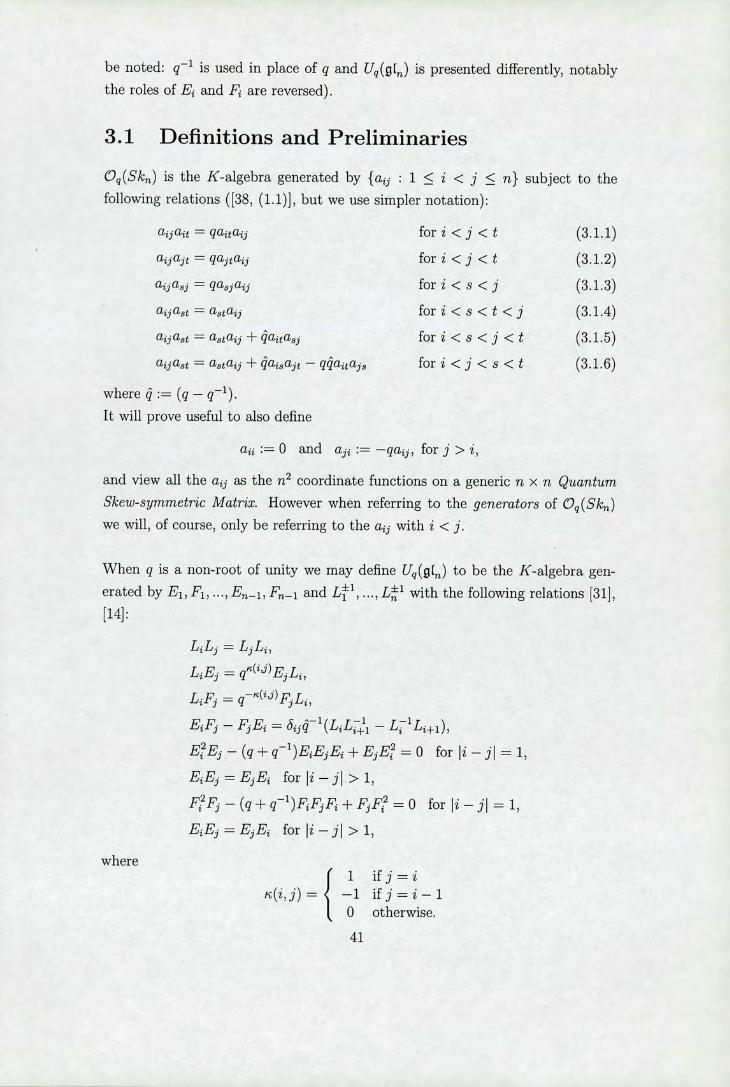
be noted: q is used in place of q and Uq(g) is presented differently, notably the roles of Ei and F are reversed).

3.1 Definitions and Preliminaries

(9q(Skn ) is the K-algebra generated by {a 3 : 1 < i < j < n} subject to the

following relations ([38, (1.1)], but we use simpler notation):

aa t = qa jta jj

aij a jt = qajtaij

aijasj qa5j a jj

aijast astai j

aijast a3 a + daitas j

aij ast a3 a + dai,,ajt - qajtajs

for i < j <t (3.1.1)

for i<j<t (3.1.2)

for i<s<j (3.1.3)

for i<s<t<j (3.1.4)

for i<s<j<t (3.1.5)

for i<j<s<t (3.1.6)

where 4 := (q - q).

It will prove useful to also define

aii := 0 and aji := —qa jj , for j > i,

and view all the aij as the n2 coordinate functions on a generic n x n Quantum

Skew-symmetric Matrix. However when referring to the generators of Oq(Skn)

we will, of course, only be referring to the aij with i < j.

When q is a non-root of unity we may define Uq(() to be the K-algebra gen-

erated by E1, F1 , ..., E. 1 , F_ 1 and L 1 , ..., L with the following relations [31],

[14]:

L1L

LE = LF = E, F) - FE = - L'L 1),

E?E - (q+q)E1EE+EE,? =0 for li - il = 1,

EE = EE for i-il >1,

F2Fj - (q+q)FjFjF+Fj F 2 = 0 for Ii - i = 1,

EE = Ej Ei for Ii - jJ >1,

where 1 ifj=i

(i, j) —1 ifj=i-1 0 otherwise.

41

It is endowed with a Hopf algebra structure with comultiplication given by

L j±1 ® L' (3.1.7)

A(E) = ® 1+ LL 1 ® E (3.1.8)

z(F) = ® L'L +1 ® F (3.1.9)

and with counit and antipode as follows,

e(E) = e(F) = 0, e(L) = 1,

S(L) = L', S(E) = —L,'L 1E, and S(F) —FLL 1 .

Remark 3.1.1. There are many different presentations of Uq(gI) that are used in the literature, with the same symbols sometimes used to represent different

elements, and with no standard way of defining the Hopf algebra structure. It

is important, therefore, for us to define what we mean by Uq(g). Although Strickland does not explicitly state which version of Uq() is used in /381, it can be deduced from the proof of /38, Proposition 1.J and then verified that it is the version given above.

There is an action of Uq(g) on Oq(Skri ) defined, for i < j, as follows [38, (1.2)]:

1 0 ifi,js+1ori=j-1=s E, aij = a_1 j if i = s + 1 (3.1.10)

( a_1 ifj=s+1 and i 7 s

0 ifi,js+1ori=j-1=s Fa= ifi=sandjs+1

a,3+i ifj=s

Lsaij= aij if j,j

(3,1.12) qa jj ifz=sorj—s.

This action, defined on the generators of Oq(Sk), extends to an action on the

whole algebra, making Oq(Skm ) into a Uq(g1)module algebra. In particular, the

action of Uq(g[) on products is given by,

u(ab) = (u(a)) (U2 (b))

for u E Uq(gr), a, b E Oq(Skrj ). So, for example, the action of the F on products is given by

F(ab) = Fj(a)LT 1L+i(b) + aFj(b)

(3.1.13)

for a, b E Oq(Skn). This Uq(g[)-action on products will be used repeatedly in

proofs throughout the rest of this thesis.

In [38, (1.6)] the author makes the following definition:

Definition 3.1.2. Let 1 <i1 <2 < <i, <nfor some 1< h < [n/2]. We

define the Quantum Pfaffian [i1i2.. .i2h] inductively as follows:

Ifh= 1,

and if h> 1,

[ili2 ... i2h] :=

where i. means "remove i from the list".

Remark 3.1.3. This is the natural quantum analogue of the recursive definition

of the classical Pfaffian (see Definition 1.5.4).

Example 3.1.4. In the case n = 4 the 4 x 4 q-Pfaffian is,

[1234] = a12a34 - qa13a24 + q2a14a23.

We make the following notational definition Pfq (k) := [1./c]. When dealing with

(9q(Skn) we shall shorten Pfq (n) to Pf J. Also, when convenient, we shall make

use of the convention that odd length q-Pfaffians are zero. The use of the term

length in reference to a q-Pfaffian has the obvious meaning, so that in general

[i1 . Im] has length m and Pfq is the highest-length q-Pfaffian in (9q(Skn).

We have previously stated that the Uq (gr)-action will be utilised throughout the

proof of many upcoming results. Vital to this method will be the knowledge

of the Uq (g(n)action on q-Pfaffians. This following result, [38, Lemma 1.4], is,

therefore, key:

Lemma 3.1.5. For E3, F3 E Uq(g[) and for a q-Pfaffian [i1i2 ... 2h] e (9q(Skn), we have,

E3 ([ili2 ... i2h]) {

[il ... it-1 s it+1 ... i2h] ifs + 1 = t for some t and s it-i O otherwise

and

F3 ([ili2 ... i2h]) = { [ii ... t_i s + 1 Zt+1 ... Z2h] ifs = it for some t and s + 1

0 otherwise.

Remark 3.1.6. Although not included in the above lemma we note that trivially

we also have,

L3 ([ili2 ... i2h]) = { q[il ... i2h] ifs = t for some t

[il ... i2h] otherwise.

43

3.2 (9q(Skn) is an Iterated Skew Polynomial Ring

There is a general consensus in the literature that quantized coordinate rings are

desired to be affine noetherian domains (see, for example, [4]). Now Oq(Skn) has

been defined in terms of generators and relations, so it is certainly affine. We will

show that Oq (Skn) is also both a domain and noetherian, along the way proving

that it is an iterated skew polynomial ring.

Definition 3.2.1. We will say that a monomial a111 ...ajmjm is ordered if ik <.1k for k = 1,..., m and (i1 , j1) (im,jm) where we are using < to denote

the usual lexicographic ordering. We shall refer to such monomials as ordered monomials.

In [38, Proposition 1.1] the author states that the set of ordered monomials is

a basis for Oq (Skn). The fact that such monomials span Oq(Skn) is clear from

the defining relations. The key step is to prove that these monomials are linearly

independent. We give an alternative to Strickland's proof of this fact. Instead

of her argument we use the Diamond Lemma (see, for example, [4, 1.11.6]). We

note that there is no restriction on q needed in our argument.

Proposition 3.2.2. The ordered monomials form a basis for Oq(Skn).

Proof. It remains to show that the ordered monomials are linearly independent.

We are going to apply the Diamond Lemma so our first task is to define an appro-

priate total order, which we will denote by :~L,, among the words on the letters a 3 (1 < i <j < n). In [32, Theorem 1.4] the authors use the Diamond Lemma

to show that the ordered monomials form a basis for (9q(Mn). We will later use

this result to reduce the work that needs to be done in our case. Therefore, it is

necessary for us to take the same total order (this also saves us the task of show-

ing that our total order satisfies the requirements for application of the Diamond Lemma). To a word, a11 lid I we associate a matrix B = (b) E M(N), where bij is the number of times aii occurs in the word. For example, to the word a11a12a 1a11 we associate the matrix B with b11 = 2, b12 = 1, b21 = 3 and all other entries zero. To such a matrix, B, we associate a sequence

( b, b11, b12, ..., b, b22, ..., b) e N1+712 i,j

We well-order M(N) via the lexicographic ordering of such sequences. The or-

dering on words is then defined by first ordering via this well-order on the as-

sociated matrices, B, and then by the lexicographic ordering of the sequences (il ,jl ,i2,j2 ,..., id, id) E N2'. So, for example,

1 < < a12 < all < a12a34 < a34au < a <w a22a33a44.

44

From the relations (3.1.1).-(3.1.4) we get the following reduction system:

ait aij q'ajja jt

a ta " q'ajja jt

a83a —* qajj a33

a3ta —* aa8t

a3a —* a 3a5t —

a3ta '—* aa8t — a 3a3t + qa ta 3

for i <j <t

for i <j <t

for i < S

for i < s <t <j

for i < S <j < t

for i < j < s < t.

We note that in all cases the words on the RHS are lower with respect to our

ordering than the one on the LHS. Applying the Diamond Lemma, our proof

will be complete if we can show that all ambiguities are resolvable (for the exact

definitions of these terms we refer the reader to [4, 1.11], but it will be clear enough

from the work we do below). We must show that a word, aa3 akj, consisting of

three distinct letters can be unambiguously resolved (i.e. put into ordered form

using our reduction system). Consideration of the reduction system defined above

yields that ambiguities arise when,

a 3 > a3t > a/

where we denote by, <, the ordering induced by the lexicographic ordering in the

subscripts. Suppose I{i,j,s,t,k,lH = 4. Then one can easily show that

a,a3 ,ak1 C K(a, : u,v E {i,j,s,t,k,l}) O(Sk).

So we may as well assume that a 3 , a3t , aki E Oq(Sk4). Now from the relations

(3.1.1), (3.1.3), (3.1.4), and (3.1.5), it can be readily seen that

K(a13, a14, a23, a24) Oq(IV[2).

So if a 3 , a3t , aki E {a13, a14, a23, a241 then all ambiguities are resolvable by the

proof of [32, Theorem 1.4]. We are left with the cases:

z>y>a12

a34 > y> a12

a34 > y > x,

where x,y,z E {a13,a14,a23,a24}. Firstly, let us note that a12 and a34 both q-

commute with a13, a14 , a23, and a24. Secondly, we note that

Zy =

for some y, z, e {ai3, a14, a23, a241, .X j E K. Now, using our reduction system,

{ z(qai2y) --+ q'(q'ai2z)y -* q -2 a12(E j Ayz1), zya12 :

Ayz)ai2 .' E j jyj(q'a12zj) .' q -2 a12(E j Ayz).

So ambiguity (i) is resolvable. Similarly (iii) is resolvable. We turn to (ii):

{ a34 ya12

a34(q 1a12y) - q(ai2a3 - qa13a24 + qa14a23)y, (1) (qya34)a12 .' qy(ai2aa - qa13a24 + q4a14a23). (2)

Further reductions depend on y. Suppose y = a13. Then (1) reduces as follows:

q'(a12a34 - qa13a24 + qqa14a23)a13

q' (ai2(qai3a34) - ai3(ai3a24 - ai4a23) + a14(qa13a23))

-f q 1(qa12a13a34 - a 3a24 - 2a13a14a23 + q 1(qa13a14)a23)

qaia1 a - q a 3a24 + ( 2q + q 2)ai3ai4a23

= q 2a12a13a34 - q'a 3a24 + a13a14a23 ,

where the last equality holds since qq + q 2 = 1. We now show that we obtain

the same result when we reduce (2):

qa13(a12a34 - 4a13a24 + qai4a23)

- q-1 ((qa12a13)a34 - a 3a24 + qqai3ai4a23)

= 2a12a a34 - q q 13 0 3a24 + 4a13a14 a23.

If y = a 4 then the reductions are similar to those above (except this time (2)

takes more steps and (1) less). If y = a14, a23 then y commutes or q-commutes

with everything and the equivalence of the reductions is easily checked.

Now we suppose that I{i,j, s, t, k, I 4. We will first argue that if i,j, s, t, Ic,

and 1 are such that relation (3.1.6) does not apply to aij , a3t , and aki, then all

ambiguities are equivalent to ones that are resolvable by the proof of [32, The-

orem 1.4]. Suppose (3.1.6) does not apply to aij , a8t , and aki. Then, when we try

to put the monomial aa3 ak1 into ordered form using our reduction system the

reductions that we use only involve commutation, q-commutation, and relation

(3.1.5). Apart from the q-commutation due to (3.1.2), these are all particular

instances of the relations that define (9q(Mn). Immediately we may deduce from

[32, Theorem 1.4] that if (3.1.2) does not apply then all ambiguities are resolvable.

If (3.1.2) does apply then the resolution of the ambiguities is entirely similar to

cases covered by [32, Theorem 1.4].

We now consider cases to which (3.1.6) applies. There are many such cases

and we do not explicitly go through all of them here, instead we show that the

ambiguity is resolvable in one of the more complicated examples. Consider the monomial a45a13a12. Then one possible reduction is:

a45a13a12 --4 a45(q 1a12a13)

-* q'(a12a45 - a14a25 + qai5a24)a13

q'a12 (a13a45 - a14a35 + qai5a34)

- q 1 a14 (a13a15 - ai5a23) + a15(ai3a24 - ai4a23)

- q'a12a13a45 - q 1 a12a14a35 + 4al2aMaM - q 1 (q 1ai3a14)a25

+ q 12a14a15a23 + (q 1a13a15)a24 - 2(q'a14ai 5)a23

= q 1a12a13a45 - q 1 a12a14a35 + qa12a15a34 - q 2 a13a14a25

+ q 1a13a15a24.

Reducing the monomial in the other order gives:

a45a13a12 -* (aa 5 - a14a35 + qa15 a34)a12

a13(a12a45 - qa14a25 + qai5a24)

- a14 (ai2a35 - a13a25 + qai5a23)

+ qai5 (a12a34 - a13a24 + qai4a23)

- (q'a1 ai3)a45 - a13a14a25 + qa13a15 a24

- (q1a12a14)a35 +42 (q-l al3al4)a25 - q 2a14a15a23

+ q(q 1a12ai5)a34 - q 2(q 1a13a15)a24 + q22(q 1ai4ai5)a23

= q 1a12a13a45 - 4a13a14a25 + qa13a15a24

- q 1a12a14a35 + 2q 1a13a14a25 - q 2a14a15a23

+ qa12a15a34 - 2a13a15 a24 + q 2a14a15 a23

- ( - 2q 1)ai3ai4a25 + (q - 2)ai3ai5a24

- q 1a12a14a35 + qa12a15a34

= q 1a12a13a45 - q 2a13a14a25 + q 1 a13a15a24

- q 1a12a14a35 + 4al2aMaM,

and so the two reductions give the same result. This exact same argument will of

course work for all monomials aa3 ak1 with s = k < 1 <t <i <j. In a similar manner one can show that all ambiguities are resolvable. El

In [38] Oq(Skn ) is shown to be a domain. The proof, however, relies on q being transcendental. We will now show that this holds more generally.

Proposition 3.2.3. (9q(Skn ) is a domain.

47

Proof For this proof we adapt an idea taken from [4, Proposition 1.8.17]. Order

the generators of (9q(Skm) according to the lexicographic ordering of subscripts,

a12<al3<<a1<a23< ... <a,

and label them, in order, u1 = a12, u2 = a13, ..., n-1 = ai, U = a23, ..., 'Un(n_1)/2 Then from (3.1.1)-(3.1.6) we may see that,

uiuj = quu +ij U3Ut, (3.2.1) s,t=j+1

s<t

for 1 < j < i < n(n - 1)/2, where qjj E K>< and ai jE K (in-fact, qj j = 1 or q and c = O,, or —q, depending on the values of i,j,s,t). We now set u to have degree di 2. Let (9q(Skn)o = K. 1, and for d> 0, let (9q(Sk)d be the K-subspace spanned by

{ u 1u 2 Ujr : d 1 + . + di, < d}.

This clearly defines a filtration of Oq(Skn). It is also clear that the associated graded ring, gr(Oq(Sk)), is generated by the elements y, where

Yi := n + Oq(Skn)d j _ 1 c (gr(Oq(Skn)))d .

For i > j we know that uu - q jjuju j is a linear combination of products U3Ut

with j < s < t < i (where this makes sense, and zero otherwise). Now,

d3 + dt = 28 + 2' <222 + 2' 1 <2i_1 + 21 = 2(2i_1) = 2 + 2i = d + d.

So we see that in gr(Oq(Sk)), YiYj = qjjyjyj for i > i. It follows that we have an onto algebra morphism

Oq (K 2) -p gr(O(Skn)),

where q is the obvious multiplicatively antisymmetric matrix of scalars. Using

GKdim we will argue in a similar manner to the proof of Proposition 2.6.1 that

this is in-fact an isomorphism. Suppose, for a contradiction, that 7 is not an

isomorphism. Now since Oq(K 2) is a domain [4, Theorem 1.2.7], Ker7 is

a nonempty ideal containing a regular element, and so by [26, Proposition 3.15],

GKdim(Oq(KTh()/2)/Ker7) < GKdim(Oq(K ( ') /2),

and hence

GKdim(gr(Oq(Sk))) < GKdim(Oq(K )/2).

48

Now GKdim(Oq(K ) /2) = n(n —1)/2 [4, Proposition 11.9.9], so if we can show

that GKdim(gr(Qq (Skn))) = n(n-1)/2 then we will have our contradiction. Since

(.9q (Skn) is a K-algebra with finite filtration and gr(Oq(Skn)) is finitely generated,

we may deduce that

GKdim(gr(Oq(Skn))) = GKdim(Oq(Skn))

by [26, Proposition 6.6]. An easy consequence of the previous Proposition, show-

ing that the ordered monomials form a basis for Oq(Skn), is that each graded

component of Oq(Skn) (with the canonical grading) is in bijection with the cor-

responding graded component of the commutative polynomial ring in n(n - 1)/2

variables. It follows from the the definition of GKdim (Definition 1.4.1) that,

GKdim(Oq(Sk)) = GKdim(K[xi ,. .. ,x(_i1]) = n(n - 1)/2.

Hence 'y must be an isomorphism. Therefore, since Oq(K 1V2) is a domain,

gr(Oq(Skn)) is a domain, and we may deduce that (9q(Skn) is a domain by [4,

Lemma 1.12.12]. LI

Before we proceed to the main result of this section, we recall the following lemma

taken from [4, Exercise I.1.L] which we will need in its proof:

Lemma 3.2.4. Let R c S be rings, and suppose that there is a regular element

d E S such that dR + R = Rd + R and dR fl R = 0 = Rd fl R. Then there

exist unique maps T, 8 : R -* R such that T is an automorphism of R and 8 is a

T-derivation on R.

Proposition 3.2.5. Oq(Skn) is an iterated skew polynomial ring.

Proof. Let us define an ordered series of subalgebras,

B12 , B137 ..., B1 , B23 ....., B 1 ,,.,

of Oq(Skn) as follows,

Bij := K(a t : a5t <

where < denotes the ordering of the generators, aij (i < j), induced by the

lexicographic ordering of subscripts. Since the ordered monomials form a basis

for (9q(Skri ) we may deduce that that each subalgebra, B 3 , is a free module

over the preceding subalgebra with basis {a : m ~ 0}. Now B12 = K[a12].

We will show that in general Bij is a skew polynomial extension of the previous

subalgebra, B 5. Examining the relations (3.1.1)-(3.1.6), it is not hard to see that

a jj Brs + B 5 = B 5a 3 + Brs . Now clearly since the ordered monomials form a

49

basis for (9q(Skn ) it follows that Brs has a basis consisting of ordered monomials

in {a8t : a5t < ars }. The fact that, fa t : a5t a 3}, together with the

relations (3.1.1)-(3.1.6), implies ajjBrs fl Br8 = Brsaij fl Brs = 0. We have already

shown that Oq(Skn ) is a domain and so certainly aij is regular in B 3. Therefore

we may apply Lemma 3.2.4 to get Bij = Brs [a; a, r]. Hence (9q (Sk) = Bfl_1 fl

is an iterated skew polynomial ring over K. LI

We can now deduce, using Theorem 1.2.6, the following:

Corollary 3.2.6. (9q(Skn ) is noetherian.

Before leaving this section we note that the work we have just done allows us

to apply two results from [4] to our algebra Oq(Skn). These show that Oq(Sk)

satisfies certain "nice" properties of noncommutative algebras.

Firstly we recall [4, Theorem 11.7.19]:

Theorem 3.2.7. Let A be a K-algebra with a Z>o-filtration (Ad ) d>o such that

A0 = K. 1 and all Ad are finite dimensional over K. Assume that grA can be gen-

erated by homogeneous elements Yi,. . , Ym satisfying relations YiY3 qjjyjyj for

i > j, for some qjj E K<. Then A is noetherian and satisfies the Nullstellensatz.

Corollary 3.2.8. (9q(Skn) satisfies the Nullstellensatz.

Proof. Looking at the proof of Proposition 3.2.3 we immediately see that Oq(Skn)

satisfies all the conditions of Theorem 3.2.7. LI

Secondly we recall [4, Lemma 11.9.10]:

Lemma 3.2.9. Let A = K[xi ][x2;'r2 , 62]... [x fl;'7-fl , ö flJ be an iterated skew poly-

nomial algebra over K. Then A is Auslander-regular. Now suppose that for

1 <j < i <n, we have T(x) E K'xj and 6(x) E st<j Kx3x. Then A is also

Cohen-Macaulay.

Corollary 3.2.10. °q (Sk fl) is Auslander-regular and Cohen-Macaulay.

Proof. We have shown that Oq(Skn) is an iterated skew polynomial algebra over

K. It remains to show that at each stage the automorphism and derivation

of the extension are as required. However this is an immediate consequence of

U

50

3.3 A Torus Action

When studying an algebra one of the central areas of interest is its ideal theory.

In particular the composition and structure of both the prime and primitive spec-

trums. In [4, Part II] the ideal theory of many quantized coordinate rings are

investigated and numerous results are proved for certain iterated skew polynomial

algebras. In this section we quickly show that (9q(Skn) satisfies (under certain

conditions) the setup of [4, 11.5.1] which allows us to deduce many results.

14, 11.5.11:

Let A = K[xi ][x 2; r2 , 82] ... [x; m, 8m] be an iterated skew polynomial al-

gebra over K.

Let H be a group acting on A by K-algebra automorphisms.

Assume that Xi,... ,Xm are H-eigenvectors.

Assume that there exists h1, . . , hm e H such that h(x) = 'r(x) for j < i

and such that the h1-eigenvalue of xi is not a root of unity for any i.

The reason a group acting by automorphisms on our algebra is of interest is

because the study of the prime spectrum can be aided by considering its "H-

stratification". To explain what we mean by this we give some definitions and

results from [4, 11.1 and 11.21:

Definitions and Results 3.3.1. Let H be a group acting by automorphisms on

a ring R. An H-ideal of R is an ideal of R such that h(I) = I for all h e H. An

H-prime ideal of R is any proper H-ideal P of R such that in RIP any product of

non-zero H-ideals of RIP is nonzero. The largest H-ideal contained in an ideal

I in R is written

(I:H)= flh(I). heN

If P is a prime ideal in R then (P : H) is H-prime. The "H-stratum" of the

prime spectrum (specR) corresponding to an H-prime ideal J is

specR = {P E specR: (P: H) = J},

and we have an H-stratification of specR,

specR= [J specR. JEH—specR

51

Knowledge of the H-spectrum and the structure of the H-strata therefore leads

to knowledge of the prime spectrum.

We now show that Oq(Skn ) satisfies [4, 11.5.1] (when q is not a root of unity)

and then give some of the results that this allows us to deduce.

Lemma 3.3.2. When q is not a root of unity (9q(Skn) satisfies [, 11.5.1].

Proof. Condition (a) is satisfied by Proposition 3.2.5. Now instead of x1 ,. . . ,

we label the indeterminates by aij with 1 < i < j < n according to the lexico-

graphic ordering of subscripts as in the proof of Proposition 3.2.3. Let H be the

algebraic torus, (K and let H act on Oq(Skn ) by K-algebra automorphisms

as follows,

(cvi ,. .. , a) aij =

for any (o,. .. , c) E H. Then clearly conditions (b) and (c) are satisfied. Now

for (d) we label the distinguished elements of H by hij with 1 < i < j < n and

define hij to be the row vector with all entries 1 except for q 1's in the i-th and

j-th place, so for example,

h12 = (q 1, q 1 , 11 ... , 1)

(1, q 1 , 1,q', 1,,.,, 1).

So aij = q 2a jj. Since we are assuming q is not a root of unity then clearly

the h-eigenva1ue of aij is not a root of unity for any (i, j). We note that if

(r, s) < (i, A, then I Jr, s} fl {i,j} I < 1 and so for (r, s) < (i, j) we have,

f q'a 3 , if I Jr, s} fl {i,j} = 1; ars =

ars, if I{r,s} n {i,j} = 0.

Inspection of the relations (3.1.1)-(3.1.6) yields that condition (d) is satisfied. El

Theorem 3.3.3. [4, Theorem 11.5.12] Let A and H be as in (11.5.1). Then all

H-prime ideals of A are completely prime, and there are at most 272 of them.

Corollary 3.3.4. When q is not a root of unity all H-prime ideals of (9q(Skn)

are completely prime and there are at most 2 n of them.

Proof. By Lemma 3.3.2 we may apply [4, Theorem 11.5.12]. El

To deduce further results we require the following lemma.

Lemma 3.3.5. The H-action on Oq(Skn) is rational.

52

Proof By [4, Definition 11.2.6 and Exercise II.2.F], since our H is a torus it suffices

to show that the H-action on ()q(Skn) is semisimple, that is (9q(Skn ) is a direct

sum of its H-eigenspaces, and that the H-eigenvalues induce rational characters.

These are easy consequences of the definition of H and Proposition 3.2.2. LI

Theorem 3.3.6. [4, Theorem 11.6.9] Let A and H be as in (11.5.1). Assume also

that H is a K-torus and that the H-action on A is rational. There are scalars

Aij E K'< such that 'r j (x) = Aij x j for all i > j. If the subgroup ()tiJ ) c K>< is

torsionfree, then all prime ideals of A are completely prime.

Corollary 3.3.7. Suppose q is not a root of unity. Then all prime ideals of

(9q (Skn) are completely prime.

Proof. By Lemma 3.3.2 and Lemma 3.3.5 the conditions on H are satisfied. Now

in our case ) j) c (q) so assuming q is not a root of unity (.\jj) is torsionfree. So

we may apply [4, Theorem 11.6.9]. LI

Theorem 3.3.8. [4, Theorem 11.8.4] Let A be a noetherian K-algebra, with K

infinite, and let H be a K-torus acting rationally on A by K-algebra automorph-

isms. Assume that H-spec is finite, and that A satisfies the Nullstellensatz over

K. Then

primA = {locally closed prime ideals}

= {rational prime ideals}

= H {maximal elements of spec A}. JEH—specA

Corollary 3.3.9. Suppose that K is infinite and q is not a root of unity. Then

primOq (Skn) = { locally closed prime ideals}

= {rational prime ideals}

= H {maximal elements of spec jOq(Skn)}.

JEH—specOq (Sk,)

Proof. Again by Lemma 3.3.2, Lemma 3.3.5, and Corollary 3.3.4 the conditions

on H and H-spec are satisfied. By Corollary 3.2.6 and Corollary 3.2.8 Oq(Skn) is noetherian and satisfies the Nullstellsatz over K. So we may apply [4, Theorem

11.8.4]. LI

3.4 A Laplace Expansion of Pfq

Recall the expansion of the classical Pfaffian given in Theorem 1.5.5. We now

prove that an analogous Laplace expansion holds in the quantum case. However

before we do we make the following remark.

53

Remark 3.4.1. We note here a key point that will be used implicitly in the proof

of many results to come. The presentation of Uq(g() that we gave in Section 8.1

required q to be a non-root of unity. It follows that whenever we use the Uq(gt)-

action in our proofs we should also impose this condition. However, this will not

always be necessary. As in the proof of [23, Corollary 1.1], when the relations we

establish using the Uq(() -action have coefficients in Z[q, q'] we will be able to

drop the restriction on q. Our proofs will show that the relations hold in Oq(Skn)

over Z[q, q 1] and there is a natural homomorphism from (.9q(Skn) over Z[q, q 1 ] to (9q(Skn) over K which preserves the established relations.

Proposition 3.4.2. For fixed i, k 1, ..., n we have,

6 jk Pfq= (_q)3ajj{1 .J...n]

where li - k- i ifj>k

kj= j — k ifj<k.

We note that, for simplicity, we are including some redundant terms in our sum

(odd-length q-Pfaffians and elements of the form a35 both being identically zero).

Proof. Fixing k, we proceed by induction on i. We first prove the case i = i. Now

if k = i = i then the proposition reduces to the definition of Pfq since /iij - 2

for i > i. So we must prove that for k > i,

= 0.

Now, using Definition 3.1.2, with (i1 , ... ) i_2) =(I, ..,k, ..,3, ..,n) gives,

(n-2 E(—#1k'jajj[1 ... L j ... n] = -q)Akj( aij E(—q) -2

ali, [i2 ... %:, -in-21 j=1 j=2 r=2 )

,

since q-Pfaffians of odd length are identically zero we can rewrite this as,

=

j=1 j=2 r=2 jk

An application of relation (3.1.1) gives,

n n-2 =

j=2 r=2 jok

54

1 0 ifj<jr where /3jr =

1 1 .f 3 . > ir . The sum on the RHS consists of an even number

1 of terms of the form ai8ait[2 ... k ... ... t ... n] where s < t. For a given s < t, terms of

the above form appear twice, since (8, t) = (min(j,i),max(j,i)) yields the two

possibilities, (8, t) = ( j,ir ) and (s, t) = (ir,j). We prove that the sum is zero by

showing that, for a fixed pair s < t, the coefficients of ai8ait[2 ... k......f ... n] that

occur add up to zero.

There are three general cases to consider depending on the relative ordering of

k, s, t. First suppose k < s <t. We need to calculate the value of (_q)ki+2qfr

in the two cases (8, t) = ( j,ir) and (s, t) = (ir ,j). If (8, t) = ( j,ir) then we have

k <j <j Given that (i1,...,i_2) = (1,..,, ..,3,..,m) we may see that in this

case r = t - 2. This fact, together with the definitions of Ujj and I3jj, gives

= (_q)(k_1)+(t_2)_2qO

= ( )3—k+t-5

If (s, t) = (ir,j) then we have k < ir <j and so r = s - 1. Hence,

(_q)Iiki+T_2qI3i D = (_q)(t_k_1)+(8_1)_2q_1

= _(_q)S_k+t_5

So the two coefficients do indeed sum to zero.

Next suppose s < k < t. If (s, t) = ( j, ir) then we have j < k < i and so

r = t - 2. Hence,

(_q)/ki+2q/3ir = (_q)(s_k)+(t_2)_2q0

= (_q)S_k+t_4.

If (S, t) = (ir,j) then we have ir < k <j and so r = s. Hence,

(_q)Ilki+T_2qI3ir = (_ q)(t_k_1)+(s)_2q_1

= _(_q)S_k+t_4

So again the two coefficients sum to zero.

Finally, suppose s < t < k. If (s, t) = ( j, ir) then we have j < i < k and

so r = t - 1. Hence,

(_q)Pki+7 _ 2q fiir = (_ q)(3_k)+(t_1)_2q0

= (_q)S_k+t_3.

55

If (s, t) = ( r , j) then we have i. <j < k and so r = s. Hence,

(_q)/1k3+7'_2q)3ir (_q)(t_k)+(3)_2q_1

= _(_q)8_k+t_3

So the two coefficients sum to zero in all cases. Thus we have proved the base

case in our induction. Next we turn to the inductive step. Assume that we know,

= öckPfq. (3.4.1)

We wish to show that the same statement holds for c+1. Throughout the following

argument we will use Lemma 3.1.5 and Remark 3.1.6. We recall (3.1.13) and act

on both sides of (3.4.1) by F, yielding,

0 = F (E(_q)3aci [1...k...3...n])

_j (Fc,(acj )L 1 Lc+i ([l..k..3..m]) + a jF, ([lk34)) (3.4.2)

At this point we must split our argument into three cases, k = c, k = c + 1 and

k c, c + 1. First suppose k = c. Then we have,

o (F,,(a,,j)L —' L,+, ([1....3..n]) + ajF ([1....3..n]))

(_q)c (q[1....3..n]),

jc,c+1

dividing through by q, and noting that a+i,+i = 0 and [1. .. .n] = 0, allows us to

deduce the required identity,

= 0. (3.4.3)

Now suppose k c, c + 1. Then using Lemma 3.1.5 and Remark 3.1.6 we obtain

the following from (3.4.2),

o =

(

E(_)k3ac+li[1....3..n]) +

jc

where the last term on the RHS comes from the fact that, when k c, c + 1,

F([1..k..3..n]) = [i..k....n] if j = c+1 and F([1..k..3..n]) = 0 otherwise. We

56

rewrite a,+i and deduce that,

o

=(

(_)2ac+li[l..k..3..nI) +

j5o~c

and since ILk,c+1 - 1 = ,LLkc this gives,

= 0 for k c,c+ 1. (3.4.4)

Finally suppose k = c + 1. Then (3.4.2) says,

Ti

0 = (_q)1i (Fc(%)Lc 'L,+, ([1.., c 4- 1, ..3..n]) + a jF, ([1.., c 4- 1, j=1

we note that acc = 0 = [1,.., c 4- 1, ..n] and apply Lemma 3.1.5 and Remark 3.1.6,

(ac+,, j (q'[1..,c4- 1, ..3..nI) + a j

jc,c+1

multiplying through by q and rearranging gives,

=

jc,c+1

jOc,c+1

= c 4- 1, ..3..n].

jcc+1

jOc,c+1

Now if c+ 1, /-c+l,j + 1 = /lcj, 50

(_q)13a1,j[1..,c 4- 1, ..3..n]. (3.4.5)

j5E-C

We now observe that since, a,+i = (— q) 1 ac+i,c , it follows that,

ac,+i[1.., c 4- 1, ..n] = (—q) 1a +i,[1..6, c 4- 1, ..n]

c 4- 1, ..n] = c 4- 1, n],

and since /-1c,c+1 - 1 = 0 - 1 = —1 = c - (c + 1) = we have,

c 4- 1, ..n] = c 4- 1, ..n]. (3.4.6)

Adding (3.4.5) and (3.4.6) gives us,

(_q)c+1.3a+1j[1..(c4- 1)..3n] =

By our inductive hypothesis, (3.4.2), this says,

1)..3..n] = Pfq. (3.4.7)

We are now finished, for (3.4.7), (3.4.4), and (3.4.3) together give,

8k,c+1fq

thus completing the inductive step. Keeping in mind Remark 3.4.1 we see that

our proof is complete.

The proof of the above proposition only relies upon the relative ordering of the

numbers 1, ..., n. So we have in-fact proved the following more general result:

Corollary 3.4.3. Let 1 <i1 <2 < < im <n for some 1 < h < [n/2]. For

fixed r,t=1,...,2h,

=

3.5 Pfq is Central

From now on we will use the notations aij and [ii] for the generators of Oq(Skn)

interchangeably. We thus also view the generators as length-2 q-Pfaffians. How-

ever we should make clear that although we will allow ourselves to write [ii] when

j > i, for q-Pfaffians of length greater than 2, writing [i 1 i] will always imply

that i1

Recall that in the case of standard quantum matrices, Oq(Mn), we have a distin-

guished element, namely the quantum determinant, detq, that is well-known to

be central. Since, in the world of skew-symmetric matrices, we can think of Pfaf-

fians "playing a similar role" as the one determinants do in the world of general

matrices, it is natural to expect that we would also have a centrality result for

q-Pfaffians. We shall now proceed to prove that Pfq is indeed central in Oq(Skn),

a particularly nice property for an element of a noncommutative algebra to have.

Before we prove the main result of this section we require two Lemmas giving

some specific q-Pfaffian commutation relations.

Lemma 3.5.1. For <11 <...< 12m < 2m

[12] [1 .. .12m] = [1 . . . 12m] [12] + 4(_q)T_1 [u n [21i . ..lr . . .12m].

Proof We proceed by induction on rn, the base case being the relation (3.1.6) of

the algebra. Now, expanding [11 -- -12,,] using Definition 3.1.2 gives,

2m

[12][l1 ... 12m] = (_q), 2[12][111r][12112fl2]

r=2

applying relation (3.1.6) we have,

2m [12][11 ... 12m] = (_q) r_2

([111r][12] + [111][21r1 - q[11][211 ]) [12.4..12m ],

setting (u1, ..., U2m_2) = (12, .., Ir .. 12m) and applying the inductive hypothesis to

[12][ui ... 2m] gives,

[12] [11...12m] = 2m

(

2m-2

(_q)r_2 [iilr] ([12..1 ..12m][12] +

(_q)k_1[1uk ][2ul.. k..u2m2])

r=2 k=1

+ 4 [ ill ] [21r ] [12.4.32m] - q[11] [211] [12 .1; ..12rn])

and so,

(

( —q)r-2[111,] 2m

[12] [l1...12m] = [l2..4..12m][12]

r=2 2m 2m-2

+ (_q)?+1_3 17 Lt l lrj[ lUk][2U1..Uk ..U2m_2] r=2 k=1

2m 2m

+ [1l] ((_q)r_2[21r][12l2m]) +

two applications of Definition 3.1.2 gives,

2m 2m-2 [12][l1 ... 12m] = [li ... lm][12] +

r=2 k=1 2m

[11] [212.. .l2m] +

So, for our proof to be complete, it remains to be shown that,

2m 2m-2 2m (_q)r+k_3 [lilr ] [luk] [2U1..k..U2m 2] +

r=2 k=1 r=2 2m

= (_q)r_1[1l][2l1.J..12]. (3.5.1) r=2

59

We consider the RHS of this equation. Writing (ti, ...,t2m) = (2,1j ,...(,, ..,12m)

and using Definition 3.1.2 enables us to write the RHS as follows,

2m 2m 2m (_q)r_1[1l ][2l1. j;..12

] = (_q)r_1[11] ((_q)1_2[

24][t2.4 .12m])

2m 2m =

r=2 k=2

noting that t2 = 11, we may rewrite this as,

2m 2m =

2m 2m

+ r=2 k=3

So to prove (3.5. 1) it suffices to show,

2m 2m-2 2m 2m

2] = r=2 k=1 r=2 k=3

Expanding the (2m - 2)-length q-Pfaffians on both sides, using Definition 3.1.2,

gives us, as our target,

2m 2m-2 2m-2

r=2 k=1 s=2 2m 2m 2m-2

=

(_q)r+k+8_5[11][2t][11v8][v2....v2_2] (3.5.2)

r=2 k=3 s=2

where (wi, ..., W2m_2) = (2, U1 .., U, ..) U2m_2) and (vi, ..., V2m_2) = (t2, .. .12m).

Now the RHS of this equation is composed of terms of the form,

{1la][2lb][l1lc ][12..ia..%..i..l2m]

(3.5.3)

with the numbers a, b, c running through all the possible triples of distinct ele-

ments from the set {2, ..., 2m}. We will show that this is also true of the LHS of

(3.5.2). To prove the equality we will then show that, for a given triple (a, b, c),

the coefficients of the respective terms appearing on either side of the equation

are the same.

Our first step is to rearrange [111][1uk ][2w5 ]. This depends on the relative or-

dering of l,, Uk, w8 so we must split this into the six appropriate cases:

nk<ws<lr:

By (3.1.5),and then an application of (3.1.5) and (3.1.4) we have,

[111r1[lUk][2W 3 ] = ([ lUk][lllr I - [llr ] [link]) [27v5 ]

= [luk] [2w8 ] [lilr] - [1Uk] [21r ] [11w8] - [11r ] [2w5 ] [link].

W 3 <Uk<l:

By (3.1.5), and then (3.1.5) applied twice we have,

[lilr] [luk ] [2w5] = ([ink] [li lr ] - q[ll] [lluk ]) [2w5 ]

= [ink] [2w3] [lilr] - [lnk] [21r1 [11w5 ]

- q[llr ] [2w5 ] [liUk] + 42 [ilr ] [2nk] [11w5 ].

Uk<lr <Ws :

By (3.1.5), and then (3.1.4) applied twice we have,

[lilr] [ink ] [2w5] ([ink] [lilr] - q[ilr ] [lluk ]) [2w5 ]

= [1Uk][2Ws][1l1r] - [11r][2ws][11uk].

ir <w8 <Uk

Two applications of (3.1.4) give,

[lilr] [ink ] [2w5 ] = [ink] [lilr] [2w5 ]

[iu] [2w5 ] [lilr].

ws <lr <nk:

By (3.1.4) and then (3.1.5) we have,

[lilr] [ink ] [2w3] = [ ink] [ll] [2w5 ]

= [ink] [2w5 ] [lilr] - ql[iUk] [21r ] [11w5 ].

lr <Uk<ws :

Applying (3.1.4) twice gives,

[iilr] [ink] [2w8] [ ink] [lilr] [2w5]

= [ink] [2w5 ] [lilr].

Now for r = 2,..., 2m, k = 1, ..., 2m - 2, and s = 2,..., 2m - 2, (lr , nk, w3) runs

through all possible triples of distinct numbers from the set {12, 12m}. So from

(i) - (vi) it follows that the LHS of (3.5.2) is composed of terms of the required

type. It remains to show that, for a given triple (a, b, c), the coefficients of terms

of the form (3.5,3) are the same on either side of the equation. We begin by

61

calculating the coefficients of terms on the LHS, by examining the cases (i) - (vi)

above and seeing when a nonzero term of the required form arises. Again this

depends on the relative ordering of 1a 1b, l so we split this up into six cases:

1a< 1b< 1c

The only nonzero term is in (i) when (la, 1b, l) = (Uk, w, lv). We wish to calculate

the value of the coefficient which is, in this case, (_q)r+k+s_5. So we must express

r, k, s in terms of a, b, c. Let us recall how Uk, w, 1, are defined. We start with the

ordered list (12, .. - , 12,) - We remove 1, and relabel the new list (u1, ..., 112m2). We

then remove Uk and relabel the new list (w2, ..., w2m_2). And finally we remove

w3. So the values of k and s that give Uk = 1a and w8 = 1b will depend on whether

the elements removed from the lists before the respective relabelings came before

or after Uk (resp. w5 ) in the ordering. In the case we are in the relative ordering

Of I, Uk, W 8 is Uk < W, < 1, giving (r, k, s) = (c, a - 1, b - 1). So the coefficient of

the term in question is

(_q)r+k+3-5 = (__q)a+b+c-7

lb< 1a< 1c

The only nonzero term is in (ii) when (la, 1b, 1) = (Uk, Ws, ir). The relative order-

ing of 1r, Uk, w5 is w8 < Uk < 1r giving (r, k, .$) = (c, a - 1, b). So the coefficient

is (_q)r+k+s-5 = (_q)a+b+c-6

1b< 1c< 1a

In this case there are two nonzero terms. The first occurs in (ii) when (la, 1b, l) =

(Ir , w3, Uk) with coefficient _(_q)r+k+s_5; the relative ordering in this case is

W 5 < Uk < ir giving (r, k, s) = (a, c - 1, b). The second occurs in (v) when

(Ia, 1b, l) = (Uk, Ws, ir ) with coefficient (_q)r+k+5_5; the relative ordering in this

case is w3 < Ir < Uk giving (r, Ic, s) = (c, a - 2, b). So the combined coefficient is

(_q)a+b+e_7(1 + q) = (_q)a+b+c_5.

1a<tc< 1b

Again in this case there are two nonzero terms. The first occurs in (i) when

(Ia, 1b, 1) = (Uk, 1r, w3 ) with coefficient _(_q)r+k+5; the relative ordering in

this case is Uk < w5 < I,. giving (r, k, s) = (b, a - 1, c - 1). The second occurs

in (iii) when (la, 1b, 1) = (Uk, Ws, Ir ) with coefficient (_q)r+k+s_5; the relative

ordering in this case is Uk < 1,. < w8 giving (r, k, s) = (c, a - 1, b - 2). So the

combined coefficient is

(_q)a+b+c_8(q + 1) = ( _q)a+b+c_6

62

1c< 1a<lb

In this case there are three nonzero terms. The first occurs in (ii) when (la , 1b, i)

(Uk, 1r, w8 ) with coefficient _(_q)3_5; the relative ordering in this case is

W 8 < Uk < 1, giving (r, k, s) = (b, a - 1, c). The second occurs in (iii) when

(Ia , 1b, l) = (ir, w, Uk) with coefficient _(_q)r+k+s-5; the relative ordering in

this case is Uk < l < w3 giving (r, k, s) = (a, c — i, b-2). The third occurs in (vi)

when (Ia, 1b, 1) = (Uk, 'W 8 , Ir ) with coefficient (q)r+k+s.-5; the relative ordering

in this case is ir < Uk < w3 giving (r, k, s) = (c, a - 2, b - 2). So the combined

coefficient is (_q)a+b+c_9(q3 + q + 1) = (_q)a+b+c_5

1c< 1b< 1a

In this last case there are four nonzero terms. The first occurs in (i) when

(la, 1b, i) = (lv, w5 , Uk) with coefficient-4( — q)r+k+8_5; the relative ordering in

this case is Uk <w8 < I giving (r, k, s) = (a, c— 1, b— 1). The second occurs in (ii)

when (la, 1b, l) = (Ir, Uk, w) with coefficient 2(_q)r+k+s_5; the relative ordering

in this case is w3 < Uk < l giving (r, k, s) = (a, b - 1, c). The third occurs in (iv)

when (la, 1b, l) = (Uk, W 8 , lr ) with coefficient (_q)r+k+s-5; the relative ordering

in this case is I < w5 < Uk giving (r, k, s) = (c, a - 2, b - 1). The last occurs

in (v) when (la , 1b, l) = (Uk, ir , w8 ) with coefficient _4(_q)r+k+s_5; the relative

ordering in this case is w5 < 1r < 'a, giving (r, k, s) = (b, a-2, c). So the combined

coefficient is

(_q)a+b+c_s(q + q22 + 1 + q) = ( _q)a+b+c_4

Our final task is to show that in cases (1) - (6) the coefficients that we have

calculated on the LHS match those on the RHS of (3.5.2). Recall that the RHS

is 2m 2m 2m-2

(_q)r+k+s_5[1lJ{2t ][l1V8 ][v2.. j8..V22]

r=2 k=3 s=2

where (t3, ..., t2m) = (12, ...lr, .., 1) and (v2, ..., v2m_2) = (t3) .. tk, ..t2m). For a

given a, b, c the coefficient of the term of the form (3.5.3) is (_q)r+k+s_5 where

(lr , tk, v5 ) = (la, 1b, la). In case (1) the relative ordering of ir, tk, v8 is l. < tk < V3

so (r, k, s) = (a, b, c - 2) and so the coefficient is (q)a+b+c_7 as required. In

case (2) the relative ordering is tk < Ir < v3 so (r, k, s) = (a, b + 1, c - 2) and

so the coefficient is (_q)a+b+c_6 as required. In case (3) the relative ordering is

tk < V3 < 1r so (r, k, s) = (a, b + 1, c - i) and so the coefficient is (_q)a+b+c_5 as

required. In case (4) the relative ordering is 1r < v3 < tk so (r, k, s) = (a, b, c - i)

and so the coefficient is (q)a+b+c_6 as required. In case (5) the relative ordering is

63

V 3 < 1 <tk so (r, k, s) = (a, b, c) and so the coefficient is (_q)a+b+c-5 as required.

Finally, in case (6) the relative ordering is v3 < tk < 17 so (r, k, s) = (a, b + 1, c)

and so the coefficient is (_q)a+b+c-4 as required.

Lemma 3.5.2. For 2 < 11 <... <12m_ 1

[12][21, ... 12m-11 = q[211 ... l 2m_11 [12].

Proof. Now, using Definition 3.1.2 and then relation (3.1.2) we have,

2rn-1

[12][211...12m_ 1] = [12] (

(_q)k_1[21k][ll..1..l2ml])

2m-1 = (_q)k_lq[2l][12][l1....l21].

Applying Lemma 3.5.1 while setting (jr, ...,j2rn2) = (117 , 1k, ) 12m_1) gives,

[12][211...12m_ 1 ] = 2m-1 2rn-2

(_q)klq[l] ([11.4..12m 11[12] + 4 (_q)r1[1ir][2i1..Jr..i2m2]),

and by Definition 3.1.2 we can deduce

2m-1 2m-2

[12][211...12m_1] = q[2l1 ... l2m1][12]+q (_q)k+r_2[21][1j][2j1,.J..j2_2].

kzl r=1

So it suffices to show that 2m-1 2m-2

(_q)k+r[21][1j][2j1..j..j2_2] 0. (3.5.4) k=1 r=1

Now, by Definition 3.1.2,

2m-1 2m-2 (_q)k+T[21][1j][2j1..J .. j22]

k=1 r=1 2m-12m-22m-2

= (3.5.5) k=1 r=1 t=2

where (wi, ..., W2m_2) = (21 j i7 ..)J,., ..,j2m_2). We now express [21k ][1j][2wt ] in

terms of ordered monomials. This depends on the relative ordering of 1k, jr, Wt SO

we split this into the appropriate cases:

(a) 1k <Jr <Wt

By (3.1.4),

[21k ] [un] [2w] = [ljn] [21k] [2w].

64

jr<lk<Wt:

By (3.1.5),

[21k] [1j,] [2w] = ([ljr ] [21k ] - q[llk] [21'r ]) [2w]

= [1jr][21ic][2Wt] - [11k][2jr][2Wt].

Jr <Wt<lk

By (3.1.5), and then (3.1.1) we have,

[21k]{ljr ][2Wt] = ([ljr][21k] - 4[11k][2J])[2Wt ]

= q —' [1j,] [2wt ] [21k ] - q[llk] [2jr ] [2wt ].

lk<Wt <jr :

By (3.1.4),

[21k ] [ljr] [2wt] = [ljr] [21k ] [2wt ].

Wt <lk<

By (3.1.4), and then (3.1.1) we have,

[21k ] [ljr ] [2w] = [1j] [21k ] [2wt ]

= q'[1jr ][2wt ][21k].

Wt<3r<lk

By (3.1.5), and then (3.1.1) applied twice we have,

[21k][1jr ][2Wt ] = ([ljr][21k] - [11k1[2jT])[2wt]

= q-' [1j,] [2wt ] [21k] - q'{11k] [2wt ] [2jr ].

So we may express the RHS of (3.5.5) as a sum of terms of the form

with 1b < lc.

We shall show that, for a given a, b, c, the coefficients of these terms are in-fact

zero, thus proving (3.5.4). We proceed in a manner similar to the proof of (3.5.2)

in Lemma 3.5.1 and split this into cases:

la <lb <l

From (a)—(f) we have a contributing term in case (b) with coefficient (_q)k+r+t-2,

when (Ia , 1b, 1) = (jr, 1k, lilt). Noting that j, is chosen from (ii, ...,j2m_2) =

(11, ..) (, .., 12m_1) and Wt is chosen from (w2, ... , W2m_2) = (ii, .. .. 32m-2) it

follows that (k, r, t) = (b, a, c - 1). There is also a contributing term in case

65

(c) with coefficient q-1(_q)k+r+t-2, when (la, 1b, l) = (jr, Wt, ik). In this case

(k,r,t) = (c,a,b). So the combined coefficient is,

(_q)a+b+c-3 + q—l(_q)a+b+c-2 = 0.

1b < l a <l

We have a contributing term in case (a) with coefficient (_q)k+r+t-2, when

(la , 1b, l) = (jr, 1k, Wt), and so (k, r, t) = (b, a - 1, c - 1). There is a contrib-

uting term in case (b) with coefficient _(_q)k+r+t_2, with (La , 1b, l) = (1k, jr, Wt),

and hence (k,r,t) = (a,b,c - 1). Also there is a contributing term in case (f) with coefficient q_l(_q)k+r+t_2, with (la, lb, le) = (jr , Wt, Ik), and hence (k,r,t)

(c,a,b+ 1). The combined coefficient is,

(_q)a+b+c_4(1 + q - q2) = 0.

1b < l < Ia

We have a contributing term in case (c) with coefficient _(_q)k+r+t-2, when

(I a, 1b, I) = (ik, jr, Wt), and so (k, r, t) = (a, b, c). There is a contributing term

in case (d) with coefficient (_q)k+r+t-2, with (la, lb, ic) = (jr ,lk, Wt) , and hence

(k, r, t) = (b, a — i, c). Also there is a contributing term in case (e) with coefficient q_1(_q)k+7,+t_2, with (la, lb, l) = (jT, W,, ik), and hence (k, r, t) = (c, a - i, b + 1).

Finally, there is a contributing term in case (f) with coefficient q_l(q)k+r+t_2,

with (Ia , lb, lc) = (lk, Wt, jr ), and so (k,r,t) = (a,c,b+1). The combined coefficient

is, (_q)a+b+c_3(q + 1 - i - q) = 0.

101

We are now in a position to prove the main result of this section,

Proposition 3.5.3. Pfq is central in Oq(Skn).

Proof. Now, by definition,

al2Pfq = ( _q)r_2a12a1[2....fl]

= a12a12[3 ... n] +

applying Lemma 3.5.1 gives,

a12Pfq = a12 ([3 ... n]al2 + (_q)T_3alr[2....n]) +

66

and hence,

a12 Pfq = a12[3 ... n]al2+

(q - q') (_q)r_3a12a1[2....fl] +

a12[3 ... n]ai2 + (—q')

using (3.1.1) we have,

a12Pfq = ai2[3 ... n]a12 + (—q1) ( _q) r_3qa1a12 [2....m] .

Applying Lemma 3.5.2 to a12 [2....n] gives,

al2Pfq ai2[3 ... n]a12 + (—q') (_q)T_3q2a1[2. ...n]a12,

and so,

al2Pfq = (a12 [3 ... n] +Y(—q)r_2alr[2....n] a12

= Pfqal2 .

Now by Lemma 3.1.5, Fs (Pfq) = 0, and since A(F5 ) = F5 ® Ls 1L5+1 + 1 ® F5 , it

follows that,

F5 (ajj Pf q ) = F5(a jj)L'Ls+i (Pfq)

= Fs (a jj)Pfq.

Similarly, Fs (Pf qaij ) = Pfq Fs (aij ), so,

Fs (a jj Pfq - Pfqaij ) = F5(a jj )Pfq - Pf qFs (aij ).

We have shown, a12Pfq - Pfqai2 = 0. Hence,

F2(ai2Pfq - Pfqai2) = 0

F2(a12)Pfq - Pfq F2(a12) = 0

ai3Pfq - Pfqal3 = 0-

A trivial induction using the action of the Fk gives,

aijPfq - Pfai = 0, for j = 2, ..., n.

For fixed j we may then proceed in a similar manner to prove

a jj Pf q —Pfqa jj =0, for 1i<jn.

Keeping in mind Remark 3.4.1, the result follows. LI

67

We end this section with the observation that the centrality of the q-Pfaffian en-

ables us to employ another result of [4].

Recall [4, Lemma 11.9.11]:

Lemma 3.5.4. Let A be a noetherian, A uslander- regular, Cohen-Macaulay K-

algebra.

If z E A is a central regular element, then A/(z) is Auslander-Corenstein and

Cohen-Macaulay.

Assume that A = (1)')O oAi is a connected graded K-algebra. If c E A is a

regular normal element such that cAi = Ac for all i, then A[c 1 ] is Auslander-

regular and Cohen-Macaulay.

Corollary 3.5.5. (9q(Skn)/KPfq) is Auslander-Corenstein and Cohen-Macaulay

and Oq(Skn)[PJ'] is Auslander-regular and Cohen-Macaulay.

Proof. We saw at the end of Section 3.2 that Oq(Skn) is noetherian, Auslander-

regular, and Cohen-Macaulay. Given that Pfq is central and that Oq(Skn) is a

domain (Proposition 3.2.3), the conditions of the previous lemma are all trivially

met in our two cases. LI

3.6 A Link with Cq(2, n)

We now show that there is a link between Oq (Skn) and Gq (2, n). More specifically,

we will show that if we factor out the ideal generated by the length-4 q-Pfaffians

from Oq(Skn) then the resulting algebra is isomorphic to Cq (2, n). To do this

we first recall the presentation of Cq (2, n), in terms of generators and relations,

given in [12, Example (5.7)] (except we reverse the roles of q and q 1):

Cq (2, ri) is the K-algebra generated by {b : 1 < i < j n} subject to the

following relations:

bij bjt = qbb 3 ,

bij bsj = qb5 b,

bij bst = q2b3tb - + q'b 8bt ,

bij bst = q2b8tb -

Uij1)t - q 2 U5tUjj,

bij bst - qb 8 b t + q2bb = 0,

for i <j <t, (3.6.1)

for i < j < t, (3.6.2)

for i < s <j, (3.6.3)

for i<s<t<j, (3.6.4)

for i < s < j <t, (3.6.5)

for i<j<s<t, (3.6.6)

fori<j<s<t. (3.6.7)

am

Proposition 3.6.1. Let 14 be the ideal of Oq(Skn) generated by {[ijst] : 1 < i <

j<s<t<n}. Then, (9q(Skn)

Gq(2,n). 14

Proof. We define a map Gq(2, n) -f (9q(Sk fl)/I4 by bij i- where we abuse

terminology and think of the aij as generating 0q(Skn)/I4. This map is clearly

onto. We show that it is an algebra morphism. It suffices to show that the a 3

satisfy the relations (3.6.1)-(3.6.7). Relations (3.6.1), (3.6.2), and (3.6.3) are the

same as (3.1.1), (3.1.2), and (3.1.3). Since we are working in the algebra with 14

factored out we have "set the length-4 q-Pfaffians to equal zero", and so (3.6.7)

trivially holds for the aij . It remains to show that (3.6.4), (3.6.5), and (3.6.6) hold.

(3.6.4):

Let i < s <t <j. Then by (3.1.4) we have,

aa8 =

multiplying both sides by q2 gives,

q2a jjast = q2a3 a.

Since [istj] = 0 we may add a multiple of it to the RHS and deduce,

q2a jjast = q2ast a jj + q 1 [istj]

q2asta jj + q'(ajsatj - qajtasj + q2a jj ast )

= q2asta jj + q1ajsatj - daitas j + qajjast

(q2 - q)a jj ast = q2asta jj + q1ajsatj -

aijast = q2asta jj + q1aisatj -

since q2 - qq = 1. This is relation (3.6.4) as required.

(3.6.5):

Let i <s <j <t Then by (3.1.5) we have,

aijast = a3 a + daitasj .

Since [isjt] = 0 it follows that,

ai jast = a5 a + (—q 2a jsajt + q'aijast )

(1 - q 1)a jjast = a8a - q 2a jsajt

q 2a jjast = a8ta - q 2a jsajt

aijast = q2astajj -

69

and this is relation (3.6.5).

(3.6.6):

Let i <j < s <t. Then by (3.1.6) we have,

aa8 = a3 a + dai g ajt - qajta j6

= a8 a + (a 3a t - qaitajs).

Since [ijst] = 0 it follows that,

aa8 = a3 a + (q 1a jjast )

(1 - q 1)a jjasL = a,t aij

q 2a jja = a.t aij

aij ast = q2ast a jj

and this is relation (3.6.6). So the map sending bij to aij is an onto algebra

morphism. We can show in a similar manner that the map sending aij to bij is

an onto algebra morphism, and the result follows.

Corollary 3.6.2. 14 is completely prime.

Proof. We know Gq (2, m) is a domain [23, Theorem 1.41, so by the previous pro-

position (.9q(Skn)/I4 is a domain. Hence 14 is a completely prime ideal. LI

Remark 3.6.3. Let 12m (1 2m < n) be the ideal of Oq(Skn) generated by the

length-2m q-Pfaffians. In [88] Strickland shows that the previous result holds for

all 12m• However, her proof relies on q being transcendental and does not hold

in our more general setting. It is natural to ask whether this result is true when

there is no restriction on q 54 0.

Conjecture 3.6.4. 12m is a completely prime ideal for all 2 < 2m < n.

70

Chapter 4

Oq(Skn), A Different Perspective

"Quantum Skew-symmetric Matrices" are also mentioned in a paper by Noumi

[31]. The main objects of concern in the paper are certain 'quantum homogeneous

spaces', that is quantum analogues of the coordinate ring of certain homogeneous

spaces. One of these in particular is of interest to us, namely the quantum ana-

logue of the homogeneous space GL2m/SP2m. In the classical world SL2m/SP2m

can be realized as an orbit of skew-symmetric matrices. It is in exactly this

context in which Noumi refers to "Quantum Skew-symmetric Matrices". This

approach is not the same as that given in the previous chapter. We describe this

different method in the following section, extracting the relevant definitions from

Noumi's remarks.

4.1 Noumi's Approach

Let n be even, say n = 2m. Let T = be the matrix of the n2 canonical

generators of Oq(M). Let us define the following R-matrix in EndK (K72 ®K K'2),

R = E V0 eii® e 3 + 4 Ee1j ® e ji ,

1<i,j<n 1<i<j<n

where eij E EndK (K'2), 1 < i,j < n, are the matrix units with respect to the

natural basis of K'2 and ® is used here to mean the Kronecker product of matrices.

We think of R = (Rn) as an x n2 matrix whose rows and columns are indexed

by pairs (i, k) and (j, 1) respectively. For a general n x ri matrix A = (a) we

make the following notational definitions, A1 := A ® I and A2 := I ® A, where I

is the n x n identity matrix. So A1 and A2 are both n2 x n2 matrices and, if we

think of them also as having rows and columns indexed by pairs, then we have

that (A1) = aSk1 and (A2)4 = 6ak1. With this notation in place we are free

to observe that the commutation relations of the tij can be succinctly expressed

as follows,

RT2T1 = T1T2 R.

71

In [31, Section 4, pg 41] the following definition is given

Definition 4.1.1. Oq(Skn)(No) is defined to be the K-subalgebra of (9q(Mn ) gen-

erated by the following quadratic elements,

xij := (t,2k_1tj,2k - qt,2kt,2k_1).

This can also be expressed as,

X = (x)i< ,3< , X = TJTt

where J E EndK (KTh) is the matrix of a "quantized"-symplectic form defined, in

terms of the eij E EndK (K'), as follows,

J := (e2k_1,2k - qe2k,2k_1).

The relations amongst the xij are given in [31, Proposition 4.4],

Proposition 4.1.2. The xij satisfy the following relations

x=O for i=1,..,n, xjj= —qx jj for l<i<j<n,

RX2R12X1 = X1 Rt2X2R,

where R 1 is an n2 x n2 matrix with rows and columns indexed by pairs (i, k), (j, 1)

respectively, with entries given by (Rt2) := Rji .

Finally, Noumi also makes the following definition [31, Remark 4.12], which can

be seen as a quantum analogue of Definition 1.5.2:

Definition 4.1.3. Let Q, := {cr E S : o(2i —1) <o(2i) for i = 1, ...,m}.

Pfq(No) (n) 1

[m]q4! (_q)1(w)1 (1)(2)

WEn

where 1(w), the length of w, is the number of inversions in w,

1(w) = #{i <j : w(i) > w(j)}

and 1 4k M

[k] q4 := 1 + ... + q4(k_l), [m]q4! := fl[k]q4.

We note that this definition is valid only when [M] q4! 0. If we assume q is not

a root of unity then this is certainly the case.

72

Example 4.1.4. We now see what this definition means in the case n = 4.

Pfq(No)(4) = [2Iq4!12X34 - qx13 x24 + q2x14x23

- q3x24x13 + q2x23x14 + q4x34 xi2).

Contrast this with the 4 x 4 q-Pfaffian given in Example 3.1.4 in the last chapter.

Remark 4.1.5. In making the above definition Noumi observes that

Pfq(No)(fl) = detq(T).

Since detq(T) is central in Oq(Mn) and Oq(Skn )(No) is a subalgebra of Oq(Mn )

this yields the centrality of Pfq(No) in Oq(Skn)(No). This does not invalidate our

result in the previous chapter since Pfq(No) is only defined when q is a non-root

of unity.

We now generalise Noumi's definition, in the obvious way, to sub-q-Pfaffians of

any (even) length.

Definition 4.1.6. Let 1 < i1 < i2 < < i2h < n for some 1 < h < m. Let

2h := {cr E S2h : u(2i— 1) <o(2i) for = 1,...,h}. For not a root of unity,

1 1(w) [z1.. .i2h](No) := [h]

(—q) Xiw(j) iw(2) XjW (2h_1)jW (2J)

wEO2h

So from Noumi [31] we have the notions of the coordinate ring of "Quantum

Skew-symmetric Matrices" and of q-Pfaffians that are apparently distinct from

those of the previous chapter. The question arises as to how these rival concepts

are related. This matter is addressed in the next section.

4.2 The Equivalence of Strickland and Noumi

In Section 3. 1, (9q(Sk) was presented abstractly in terms of generators and rela-

tions. In the previous section Oq(Skn)( No) was defined to be a specific subalgebra

of (9q(Mn). We shall now show that these two objects are in-fact (under certain

conditions on q) isomorphic. First of all we show that, with no restrictions on q,

Proposition 4.2.1. There is an onto algebra morphism,

Oq(Skn) (9q(Skn)(No) given by aij i-* x1 .

Proof. It suffices to show the xij E Oq(Skn )(No) obey the same relations as the

aij E Oq(Skn). Comparing the relations of the aij given in Section 3.1 and those

73

of the xij given in Proposition 4.1.2 it is clear that if we can deduce relations

(3.1.1)-(3.1.6) from RX2R12X1 = X1 Rt2X2R (4.2.1)

then we are done. Now, for a given (i, k), (j, 1), (4.2. 1) says,

ik (RX2Rt2X1) = (Xi Rt2X2R).

Writing out what this means in full gives,

R(X2)cd (Rt2 )(X1 )( = (X1)(Rt2)(X2)ef

R[ ,

a,b,c,d,e,f a,b,c,d,e,f

and then,

R ik ad

ab R:sac6f1xbdxej R!Rc6kbSceXiaXdf. a,b,c,d,e,f a,b,c,d,e,f

Taking into account the Kronecker deltas, we deduce,

R ik Rj al Xi,ciXej R[R R ad ek xiaxci1 (4 2 2)

a,b,d,e a,d,e,f

We now look to eliminate terms in (4.2.2) which are always zero, no matter the

value of (i, Ic), (j, 1). To do this we translate the definition of R given in (4.1.1)

into a more usable form,

q, i=j=k=l;

R k = ' = j =1; (4.2.3)

q, i=1<j=k; 0, otherwise.

We now examine the LHS of (4.2.2) taking into account (4.2.3). We see that Rik is nonzero when (a, b) = (i, /c), (k, i); note that these two possibilities are ab

distinct only when k i. Suppose (a, b) = (i, k) then R ik Ral = R ik ik R and

this is nonzero when (e, d) = (i, 1), (1, i); once again note that these two cases

represent two distinct terms only when i 1. We proceed in this manner, taking

into account all the possible cases, to eliminate all the terms on the LHS and

RHS of (4.2.2) which are identically zero. After some careful thought, we deduce

from (4.2.2) that,

Rik iiRxklx + (1 - öj)Rik 1%Rxkxjj + (1 - 6jk)RkRkixiixkj

+ (1 - 41)(1 - àki)RkRikXikX1j = RR XXkI + (1 -

+ (1 - öjj)RRxjlxkj + (1 - 8)(l - 6k1)RjkRjXikX1j. (4.2.4)

74

Recall the remaining relations from Proposition 4.1.2,

Xii = 0 Vi, Xji = —qx jj for j > i. (4.2.5)

We complete the proof by examining (4.2.4) under various restrictions placed

upon the values of (i, k), (j, 1), using (4.2.5) and (4.2.3) to simplify the resulting

equation.

(i,k),(j,l) = (i,i),(j,t), i <j <t:

(4.2.4) gives,

ii it+ = + t xiixjt

++ Rti R%x1 x

qxjt xjj =

This is relation (3.1.1).

(i,k),(j,l) = (i,j),(j,t), i <j <t:

(4.2.4) gives,

+ + 31 +

= + +

xjtxij + 4q 2 xij x jt - 2qx jj x jt = qxij xjt

xjtxij = (q + q2q - q2)xjjxjt

xijxjt = qxjt xij.

This is relation (3.1.2).

(i,k),(j,l) = (i,$),(j,j), i <s <j:

(4.2.4) gives,

8 Z3 + RRx51x + + 8z 3S 28 33

- p3 5 p33 psi pu

- (is X i3 X s3 xi,xjj

xsi xii + 4xij xsj = qx jj xsj

X s jXj = (q -

= qx5jxjj.

This is relation (3.1.3).

75

(i,k),(j,1) = (i,$),(j,t), i < S <t <j:

(4.2.4) gives,

is it st xij + + RRx t x5 + RRx5xt

- RRxx5t + + Rts Rx t x 5 + RR%x5xt

XXjj - qx jsxtj + 4xitxs j + 42XisXt =xijxst - qxisxtj + qXitXs j + 42Xis xtj

xstxii = xiixst.

This is relation (3.1.4).

(i,k),(j,l) = (i, s), (j,t), i <s <j <t:

(4.2.4) gives,

Ris itRx5c x + RRx5 xt + RRxtx3 + RRx 5 xt

- RaSRJt x ji xst + RRx5xt + RR%xx 5 + RstRtJxj5xtj ts jt - is jt

xx + dqx 5 x + qX,tXsj - 2qxjsxjt = XX + qX 5 Xjt

Xij Xst = x 5 x + (q2 - 2q - )xj5xit + qxit x., j

xiixSt = xStxii + dxitxsj.

This is relation (3.1.5).

(i,k),(j,1) (i,$),(j,t), i <j <s <t:

(4.2.4) gives,

RRx5t x + R::Rx5xt . ± RisRSstt xit xsi + RRx 5 xt 3 Si

- RRit R x - is .tri5t + RRx35 3t Z5 x t + Rts tx5 + RRx 5 xt

x 5 x + qx5xt - qxjtxjs - 2qxj5xjt = xijxst

xstxji + (q - 2q)xjsxjt - qxjtxjs = xiixst

x5 x + 4xisxjt - qxjtxjs = xijxst

This is relation (3.1.6).

Our proof of the existence of an algebra isomorphism between Oq(Skn) and

0q (Sk) (No) relies upon the following well-known theorem ([31], [38], [32] ,[34], [30])

concerning the representation theory of Uq(g[). Before we state the theorem we

require some definitions. In what follows, unless stated otherwise, modules will

be assumed to be left-modules.

76

Definition 4.2.2. Let M be a Uq(g[)module. Let m E M. We say m is a

weight vector with weight ) = (A,,..., An), if, for s = 1, ..., n, L3m = qm where

A,, e Z. Furthermore, we say m is a highest weight vector if we also have that

Ekm=O fork= 1,..,n-1.

Definition 4.2.3. Let M be a Uq()-module. We say M is a weight-representation

Of Uq(g() if it has a K-basis of weight vectors.

Theorem 4.2.4. Let q be a non-root of unity. The finite-dimensional irredu-

cible weight-representations of Uq(J) have the same indexing and characters as

in the classical case of CL,-,. That is any finite-dimensional irreducible weight-

representation of Uq(gI) is isomorphic to some V(A) with A E where V(A)

is the unique irreducible Uq (() -module generated by a highest weight vector with

weight A, P is the weight lattice for GL, that is the free Z-module of rank n with

canonical basis (€)<j<,, and P is the set of dominant integral weights in P,

that is

P={A=A,,e,,EP:Ai >...>A}.

We now require some results concerning the representation theoretic properties

of Oq(Skn) and Oq(Skn)(No) . So far we have not defined a Uq(91)-action on

0q(Skn)(No) . In [31] Noumi gives the Uq(9)-bimodu1e structure of Oq(CLn)

in terms of, so called, L-operators. It can be checked that these right and left

Uq(g[n)-actions are exactly those that are specified explicitly in his earlier joint

paper [32, (1.35.a),(1.35.b),(1.35.c)]

Lstij = = q5 't, (4.2.6)

= tijE,= (4.2.7)

= 68 t +1 , t1 F,, = (4.2.8)

where the L,,, E,,, and F,, are the generators of Uq(g) and the tj are the gen-

erators of Oq(Mn), thought of as a subalgebra of Oq(CL) (we shall implicitly

regard Oq (Mn) as a subalgebra of Oq(CLn) hereafter). With this Uq (grn)-action

(.9q (Skri )(No) is easily seen to be a right Uq (g[n)-module. However the result we

shall use concerning the representation theory of Oq(Skn) is in the context of it

being a left Uq (grn)-module. This problem can be overcome, for there is in-fact

another subalgebra of Oq(CLn) which is isomorphic, as an algebra, to Oq(Skn )(No)

[31, Remark 4.5]. We shall call this algebra Oq(Sk fl) N0). It is defined by Noumi

to be the K-subalgebra of Oq(M) generated by the quadratic elements Yij defined

by

Y = (Yij)i<i,j<n, Y = TtJ_1T. (4.2.9)

77

The algebra isomorphism is given by x -+ Yij. This different subalgebra is indeed

a left Uq((n)module under the stated action. In [31] Noumi states the following

representation theoretic result relating to Oq(Skn) N0) .

Proposition 4.2.5. [31, Remark 4.5] Let q be a non-root of unity.

Let (Oq(Skn) No) , detq(T) 1) be the subalgebra of (.9q(CLn ) generated by the yj3

and detq(T) 1 . Then we have the following multiplicity free decomposition as a

Uq (9t)module

(Qq(Skn ) No) ,detq(T) 1 ) V(A) A E P,+

where

P={EP:A=br A2r,br EN for r=1,...,m-1 and bm EZ}

denoting the fundamental weights by Ar =

We may use this result to prove the following decomposition of Oq(Skn) No) .

Lemma 4.2.6. Let q be a non-root of unity. As a Uq(j) -module Oq(Skn ) 0)

has the following decomposition

Oq (Skn) No) V)

AEPs

where

P{EP br A2r , br N for r1,...,m}

and each irreducible component occurs with multiplicity one.

Proof. Now from (4.2.9) it follows that the yjj are given explicitly by

yij = (t2k,it2k_1, - q't2k_1, t2k, ). (4.2.10)

From (4.2.6) it follows that all the weights on Oq(Sk fl) 0) are nonnegative. Fur-

thermore it easily follows from (4.2.6) that all positive weights in P are possible

on Oq (Skn) No). The result then follows from the previous proposition. El

Remark 4.2.7. We note that this decomposition into irreducibles is exactly the

same as in the classical case (i.e. the coordinate ring of skew-symmetric matrices

decomposes as a CL-module into irreducibles indexed by P5 /18, Proposition

4. 21).

We now turn to (Dq(Skm). Strickland proves that it too decomposes analogously

to the classical case.

Proposition 4.2.8. [38, Proposition 1.3] Let q be a non-root of unity. As a

Uq(g[) -module (9q(Skm) has the following decomposition

Oq(Skn) V(\)

where each irreducible component occurs with multiplicity one.

Remark 4.2.9. We note that this is not the phrasing of the proposition as stated

in [881. However it is exactly the same result translated into the notation we are

using.

We are now in a position to prove the following,

Proposition 4.2.10. For q not a root of unity,

Oq(Skn) Oq(Skn )(No).

Proof We have the following onto algebra morphism by our work above,

W Oq(Skn) Oq(Skn ) No) given by Yij.

One can check from (4.2.6)-(4.2.8) and (4.2.10) that U,(,,) acts on the Yij in

exactly the same way as it acts on the aij (as given in (3.1.10)-(3.1.12)). Hence IF

is clearly a Uq(91)-module morphism. It follows that KerW is a Uq(gJ) -module.

Suppose KerW 0. Then by Proposition 4.2.8 there must exist a 'y E

such that V(-y) c KerW, where V(-y) is an irreducible Uq(g()-module that oc-

curs once in the decomposition of Oq(Skn). That is W(V('y)) = 0. But by

Lemma 4.2.6 Oq(Skn) NQ) has the same decomposition into irreducible Uq(g()-

modules as Oq(Skn), with each irreducible component also occurring once. So

'IJ(V('y)) = 0 contradicts the surjectivity of IF. Hence KerW 0 and we have

shown that W is an isomorphism.

Now that we can view the xij and aij interchangeably (for q not a root of unity)

we may apply our original definition of a q-Pfaffian, Definition 3.1.2, to the x j

and ask whether it is related to Noumi's q-Pfaffian. We first consider the case

n=4.

Lemma 4.2.11. For q not a root of unity,

[1234](NO) = [1234].

79

Proof.

[1234](N ) - 1 (x12x34 - qx13 x24 + q2x14 x23

- q3x24x13 + q2x23x 14 + q4 x34 x 12).

We rewrite this using (3.1.5), (3.1.4), (3.1.6), and Definition 3.1.2,

[1234](N0) = [21q4!U] - q3 (x13x24 - qx14x23) + q2x14x23

+ q4(xi2x34 - x13x24 + qx14x23))

1 - ..--([1234] + q4 (x12x34 - qx13 x24 + q2xi4x23)) - [2]q4!

1 - -(1 + q4)[1234] - [2]q4!

= [1234].

We now prove that the two q-Pfaffians are equal in general.

Proposition 4.2.12. Let 1 < i1 <i2 < <i2h <nforsome 1 < h m. For

q not a root of unity,

[il...i2h](No)

Proof. We proceed by induction on h, the base case h = 1 being trivial. We

note that the proof of Lemma 4.2.11 translates directly into a proof of the case

h = 2. So we may assume h > 2. With this assumption in place we now prove

the general inductive step. By definition,

[i1 ... 2h](No) = {h] 4T (_q)l(W)xij

q WEQ2h

Recalling that Q,, := {a e S : a(2i - 1) < o- (2i) for i = 1, ..., m} allows us to

rewrite the above equation as,

2h-1 2h [il ... i2h](No) = xiij

(_q)l(W) X (3) (4)

jq4' s=1 j=s+1 wE(12h W(1)=s w(2)=j

(4.2.11)

We will attempt to rewrite the sum in brackets in such away as to allow us to

apply the inductive hypothesis. Fix w(1) = s < j = w(2). Let (li, ..., 12h2) =

(i1) ..,i,..,i,..,i2h), that is,

{ k, 1k<s;

Ik k+1, s k <j - 1; (4.2.12) k+2, j-1k2h-2.

80

Define w' E 2h-2 by

( w(k+2), 1<w(k+2)<s; w'(k) = w(k+2)-1, s+1 <w(k+2) <j; (4.2.13)

1w(k+2)-2,j+1_<w(k+2)_<2h.

We will now express 1(w) in terms of l(w"). By definition,

1(w) = #{i <j : w(i) > W(j)J.

This can be expressed equivalently as,

1(w)E #{w(t) <w(r) : r < t},

so,

1(w) = #{w(t) <w(1) : 1 <t} + #{w(t) <w(2) :2 <t}

+#{w(t) <w(r) : r <t}.

We are assuming that w(1) = s < j = w(2), so we have,

1(w) = #{w(t) <s: 1 <t} + #{w(t) <j :2 <t} 2h-2

+ #{w(t) <w(r + 2): r +2 < t}.

Now the relative ordering of w(3),..., w(2h) is "the same" as w'(1),..., w'(2h - 2)

by definition of w'. So

2h-2 2h-2

#{w(t) <w(r + 2): r + 2 <t} = #{w'(t) <w'(r) : r <t}.

Hence, 2h-2

1(w) = (s —1) + (j —2) +Y, #{w'(t) <w'(r) : r < t}.

But by definition of 1(w") this is just,

1(w) = 1(w") + s + j - 3. (4.2.14)

Using (4.2.12), (4.2.13), and (4.2.14), we may rewrite the sum in brackets on the

RHS of (4.2.14) and deduce that,

[il ... i2h](No)

2h-1 2h 1 3+_3

= [h]q4! - xtsij (q) (_q)1(W' )xi,1, . . .

S=1 j=s+1

By the inductive hypothesis it follows that,

2h-1 2h 1

( — q)xjj. ([h - l}q4!{11...12h_2]), [i1...i2h](NO) [h]q4! =1 3=8+1

so, 21i

[h_1}q4 h-1 2

ç- [il...i2h](No) [h] 4! '

(_q)s+i_3xjj [i1..ii..i2h]. q 8=1 j=s+1

Writing the s = 1 term separately we have,

[il ...i2h ] (No)

= [h]q4 (_qi_2xiiij [i2..i..i2h] + 2

and by Definition 3.1.2 this is just,

2h-1 2h

> (_q) S+_3 [i1....i..i2h])

s=2 j=s+1

72h-1 2h

[Z1 ... 2h](No) = Ih'4 ([1...2h] + (_q)S+i_3xjj. [i1.....i2hJ). (4.2.15)

jq 8=2 j=s+1

Suppose

2h-1 2h (_q)8+33. [i1..i..i..i2h] = q4 [h - 1] q4 [il ... i2h]

(4.2.16)

s=2 j=s+1

Then (4.2.15) would give,

[il ... i2h](No) = 1 ([il ... i2h] + q4{h - 11q4[il ... 22h])

[h] q4

1

= [il ... i2h] (1 + q4[h - 1] q4) [h] q4

1

= [i1 ... i2h] (1 + q4(1 + q4 + ... + q4(h_2))) [h]q4

1

= [i1 ... i2h] (1 + q4 + ... + q4(h_l)) [h]q4

1. = —[zl...i2h] ([h]q4)

[h]q4

=

and the proof is complete. So it suffices to prove (4.2.16).

Now, writing (li, ..., 12h-2) = (i1, .., .. i3, .., i2h) allows us to express the LHS

of (4.2.16) as follows,

2h-1 2h 2h-1 2h

E 1:(—q)33xj j . [i1..i;..i;..i2hI = E (_q)S+i_3xjj [11...12h_2]. s=2 j=s+1 s=2 j=s+1

82

Using Definition 3.1.2 this gives,

2h-1 2h

(_q)8+i3xji, [i1.f....i2h]

s=2 j=s+1 2h-1 2h 2h-2

=(_q)s+i+r_5xii.x111 {12.4..12h_2]

s=2 j=s+1 r=2

2h-1 2h 2h-2 ( _q)s+i+r_sxjj.xj11[j2..i..i;. f,..i2 J .

s=2 j=s+1 r=2

(4.2.17)

We proceed by rewriting the RHS of (4.2.17) in terms of ordered monomials. Now

i1 < i3 < ij and i 1 < l, so when we rearrange there are three cases we

must consider:

< 1, < j5 < i3 by (3.1.6), x j,jj x jj j,= X 11Xjj j - qxj1 xt r ji +

< is < 1, < i j by (3.1.5), = x 1 - 4x j1 x j j.

(iii) ji <is <j j < ir by (3.1.4), X j Xj l lr =

So we can see that when written in terms of ordered monomials the RHS of

(4.2.17) is a sum of terms of the form

XjijaXjbjc[Z 2• i •ib••iC•• Z 2h]

with a = 2,..., 2h, b 2,..., 2h - 1, and c = b + 1, ..., 2h. For a given (a, b, c) we

now calculate the coefficient of such a term in each of the three appropriate cases.

a < b < c :

Examining (i) - (iii) we see that the only term that arises occurs in (i) when

(ia, ib, i) = ( Ir , i5 , i3 ). In this case r a so the coefficient is

(_q)S+3+T_5 = (_ q)a+b+c-5

There are two such terms that arise. One occurs in (i) when (Ia, ib, i) = (is , 1" i)

with coefficient _(_q)8+i+r_5; in this case r = b. The other occurs in (ii) when

(ia , i, i) = (Ir , i5 , i) with coefficient (_q)S+i+r5; in this case i5 < 1,. < ij 50

r = a - 1. So overall the coefficient is

(_q)a+b+c_6(q + 1) = (_q)a+b+c_4

Three terms of this form arise. One occurs in (i) when (Ia, 47 i) = (1j) 1r, i5 ) with

coefficient q(_q)s+i+r_5; in this case r = b. The second occurs in (ii) when

(ia, ib, i) = (ii , i, Ir ) with coefficient _ 4(_q)5 +i'-5; in this case i, < 1 < i8 50

r = c - 1. The third occurs in (iii) when (Ia , ib, i) = (lr , i5 , i) with coefficient (_q)s+i+r_5; in this case i5 <Zj < Ir so r = a - 2. So overall the coefficient is

(_q)a+b+c_7(q3q + q + 1) = (_q)a+b+c_3.

1, a<b<c; So, defining 9abc = 4, b < a < c; ,we may deduce from (4.2.17) and the work

1, b<c<a. just done that,

2h-1 2l (_q)s+33xjj. [i1..i5..i j..i2 ]

s=2 j=s+1 2h 2h-1 2h

= (_q)a+b+c_obcxj1j Xjbj [i2. •b• .i. .i2h],

a=2 b=2 c=b+1

so,

2h-1 2h

s=2 j=s+1 2h 2h-1 2h

= (_q)a+2xi1j a=2 b=2 c=b+1

Writing (u1, ..., u2h_4) (i2, .. , .., , .., i', .., i) and using the inductive hypo-

thesis gives,

2h-1 2h

(—q)x [il..iT3..i..i2h]

s=2 j=s+1 2h 2h-1 2h

-—q)a+2 Xjija [(_q)b+c_(Oabc+2)xjj x - ( '

a=2 b=2 c=b+1 1

x(—q)1 XU (1)U (2) Xu(2h_5)u(2h_4)]. (4.2.18) [h - 2]q4! c7EO2h_4

Now let (vi, ..., V2h_2) = (i2) .., .., Z2f) and define a' E 2h_2 so that Va'(l) =

= i, and V'(r) = Ug(r_2) for r > 2. Then,

2h-2

E #{O-'(t) <a'(r) : r < t}

= #{a'(t) <a'(l) : 1 <t} + #{a'(t) <a'(2) : 2 <t}

2h-2

+ E #{a'(t) <a'(r) : r

and similarly to our earlier calculation of 1(w) we find that,

1(a') = 1(a) + #{a'(t) <a'(l) : 1 <t} + #{a'(t) <a'(2) : 2 <t}.

Since (vi, ..., V2h_2) = (i2, ..) .., and V,J(i) = i5, V0'(2) = ic the value of

#{a'(t) < a'(l) : 1 < t} + #{a'(t) < a'(2) : 2 < t} will depend on the relative

ordering of a, b, c.

a<b<c: 1(9')=1(a)+(b-3)+(c-4).

b<a<c: l(a')=l(a)+(b-2)+(c-4).

b < c < a : 1(a')=l(a)+(b-2)+(c-3).

So, 1(a') = 1(a) + b + c - (°abc + 2). Hence from (4.2,18) we may deduce,

2h-1 2h (_q)S+_3rjj [i1....i..i2h]

s=2 j=s+1 2h 1 2h-1 2h

+2 = (_q)a '" [h - 2]q4!

[x C x b=2 c=b+1

x (_q)l')xv,(3)v,(4) xv,(2h3)v/(2h2)11

V(1) =ib

and so,

2h-1 2h

s=2 j=s+1

= (_q)a+2xi1i [hq4! (

a=2

(_q)1 ')xv,(1),(2) . . . xV/(2h_ 3)V/(2h_2))

By the inductive hypothesis applied to the sum in the brackets we have,

2h-1 2h 2h

(_q)S+i_3x jj. [j1.. j .. j;., j2 ] (_q)a+2xi1i - 21q4![v1 ... v2h_2] s=2 j=3+1 a=2

= q4 [h - 11q4 (_q)a_2xi1i [i2.-Z, ..22h]

= q4 [h - 1] q4[il ... i2h].

So (4.2.16) is proved and we are done. EM

Corollary 4.2.13. For q not a root of unity,

Pfq = Pfq(No).

Ry

Remark 4.2.14. We end this section by noting that, when q is not a root of

unity, we are now in a position to view (9q(Skn) as a subalgebra of Oq(Mn). It

is natural to ask what properties of Oq(Skn) can be deduced from its relationship

with Oq(Mn), a much-studied object. We give one answer to this question in the

next section.

4.3 Another Laplace-type Expansion

Laplace expansions for quantum minors in Qq(M) are well known [32]. We use

these known expansions and our realisation of (9q(Skn ) as a subalgebra of (9q (Mn )

to produce a Laplace-type expansion for q-Pfaffians which mirrors a classical res-

ult.

Let us first fix some notation. For I = {i1 < ... < i}, J = {ii < ..• < jr} c { 1, ..., n} let denote the quantum minor of Oq(Mn) with rows I and columns

J. That is, (_ 1"t..............

a ESr

Define the symbol sgnq(I; J) as follows,

sgnq(I;J) -{ 0, ifIflJø;

- (_q)l(I;J), if I fl J = 0,

where 1(1; J) = #{(i,j) i E I,j E J,i > j}.

Finally, for I = {i1 < < '1/} c {1, ..., n} we denote [il ... i2h] by [I]. With all

this notation in place we may begin to gather the necessary results for our proof.

Proposition 4.3.1. Let q be a non-root of unity. For I = {i1 < < i2,.1 c {1,...,n}.

[II(No) ii: e2k1-1,2k,.....2kr1,2kr 1<ki<<kr<m

Proof. From Noumi [31, (4.43) and (4.59)] we have that,

(v11 A vj A ... A vi, A Vjr 0 Xii ji ... Xir jr ) 11<jl; ... ;lr<jr

= [r]q4! (, A ... A v82 0 22k1 .... .2krl2kr) (4.3.1) S1<<52, 1<ki<<kr<m

where the vi are the canonical generators of the quantum exterior algebra Aq(V) with relations

vAv=0(1<i<n) and vAv=—qvAv(1 <i<jn).

EM

Rearranging the LHS of (4.3. 1) into a sum of terms of the form v31 A ... Av32 with

Si < < S. and then equating the term v 1 A ... A v 2 ® * with the respective

term on the RHS gives us the result. El

The known Laplace expansion of Oq(Mn ) that we shall use is taken from [32]. We

note that in that paper the ground field is taken to be C however the argument

used is valid over any field.

Proposition 4.3.2. [32, Proposition 1.1] Let r, r1, r2 be positive integers with

1 <r <n and ri+r2 = r. Let and be subsets of{1,...,n} with #I = # J = r.

Let Ji, J2 be subsets of J with #Ji = r1, #J2 = r2 . Then,

1(Ij sgnq(Ji;J2) I2)cI1cI2J1 J21 = (—q)

11u12=I

where the summation ranges over all partitions I Li 12 = I such that #11

r1 , #12 = r2 .

Finally, before we proceed, we state the following combinatorial result taken from

[37, Proposition 1.3.17] which we will need,

Lemma 4.3.3. Let em,d := {(ai , ..., am) : d of the ai are 0 and m - d are 1}.

For it = (ai , ..., am) E E5,,d define inv(ir) #{i <j : ai > a}.

[m] 4imv(r) d q4 Ernd

[mI [mIg4! where I

[d q4 [dIq4![m-dIq4!•

We now have all the tools necessary to prove the main result of this section.

Proposition 4.3.4. Let q be a non-root of unity. Let n = 2m. Let 1 < d < m.

[

m]Pf, (n) = E(—q)1 [a(1)...u(2d)][a(2d+ 1) ... a(n)]. q4

a(2d-I-i)<<o(n)

Proof. Fix 1 < d < rn and let s = 'in - d. The following summation will be

restricted to disjoint subsets I, J of {1, ..., n}. Now,

(_q)l(I;J) [I] [J] = (_q)l(I;J) [I](NO) [J](No),

#I=2d #I=2d #J=23 #J=2s

using Proposition 4.2.12. We now apply Proposition 4.3.1,

:: (_q)i(I;J)[i][J]

#I=2d #J=2s

= (q)1

( e2k1 1 ...2kd) ( 21) #I=2d 1<kl<...<kd<m 1<1i<...<1<rn #J=28

rearranging the RHS gives,

Ik 1: (_q)l(I;J)1_12kde2ll-1.....2l #I=2d 1<kl<<kd<m #I=2d #J=2s 1<li< ... <18<m #J=23

An application of Proposition 4.3.2 gives,

sgn(K; L)E", #I=2d 1<kl< ... <kd<m #J=28 1<1i< ... <t<m

where K = {2k1 - 1,2k1,...,2kd— 1,2kd } and L = {211 - - 1,2l}.

Now detq(T), SO,

(—q)1'[i][J] (_q)l(KL)

#I=2d #J=28 1<li< ... <l 5<m

KflL—ø

applying Remark 4.1.5 gives,

(—q)1 '[i][J] = (_q)l(KL) Pfq(No). #12d #J=2s

1<ki< ... <ka<m

KflL=O

Using Proposition 4.2.12 we can deduce,

(—q)1 '[i][J] = E (_q)l(K;L) Pfq. (4.3.2)

#I=2d #J=25

1<kl< ... <kd<m 17<11<...<t<m

KflL=ø

Now, recalling that we are restricting our summation to disjoint subsets I, J of

{1, ..., m}, it is not hard to see that,

(_q)l(1J)[I ][ J ] = (—q)[a(1)...u(2d)][a(2d+ 1) ... cr(m)].

#I=2d uESn #J=2s o(1)< ... <cr(2d)

(4.3.3)

88

Combining (4.3.2) and (4.3.3), all that remains of our proof is to show,

(_q)l(KL) - [ml

1<kl< ... <kd<m [d]q4

lli< ... <15<m KnL=0

We use Lemma 4.3.3 to reduce the problem to showing that,

:i: (_q)l(K;L) = 4inv(ir)

1k1< ... <kdm lrE'Sm,d 1<ti< ... <1<m

KflL=O

Now, (_q)l(KL) = (_q)i(K;K) ,

1<kl<'"<kd<rn 1<11<••<18<m

KnL=ø

where K = {1, ..., n}\K. We can define abijection between '5m,ci and {(k1, ..., kd)

1 <k1 < ... <kd m} in the following obvious way,

{(kl,..., kd) :1<kl< ... <kdrn} —*Sm,d

(k1) ..., kd) I" 7rk1 .....kd

where

{ kd = (ai, ..., am), with ai

0, if i = k j for some j; 1, otherwise.

So clearly all that remains to be shown is 1(K; K) = 4inv(7rk1kd). For clarity

let us recall the following notation,

K={2k1 -1,2k1,...,2kd -1,2kd },

k={211 -1,211,...,213 -1,213 }.

{Therefore we may write ai 0, ifi=k3 for some j;1, if i = 13 for some

since {k1, ..., kd} and

{1, ..., l} partition {1, ..., m}. Hence,

inv(7rk1 kd ) = #{i < j : ai > a}

#{i <r : aj > ar }

d

: ki >l}. (4.3.4)

By definition,

l(K; K) #{(k, 1): k e K, 1 E K, k > 1}.

The RHS of this equation, taking into account the definitions of K and K, may

be expressed as follows,

d

1(K; k) = (#i : 2ki > 211 + #{i :2ki > 21 - 11

+ #{i : 2k - 1 > 2l} + #{i 2k - 1 > 21 - i}). (4.3.5)

Now

ki > l 2ki > 21 2k —1> 21 —1

and since ki and l j are distinct integers we also have

ki >l k— 1/2>13 2k —1> 21

and

>21-1.

So (4.3.5) may be rewritten as,

l(K;k) =4#{j: ki > l},

and so by (4.3.4),

l(K; K) = 41riv(7Fk1 ,...,kd).

N

Remark 4.3.5. We note that this result serves as a q-analogue for Proposi-

tion 1.5.6 which holds in the classical case.

90

Chapter 5

Further Properties of Oq(Skn )

In the classical case, relations amongst Pfaffians are central to the understanding

of skew-symmetric matrices and so-called "Pfaffian varieties". In-fact, in papers

such as [7, Section 6], [2], and [11], the use of such relations is key. In the

quantum world much work has been done on understanding quantum matrices

and the associated quantum determinantal ideals through the use of quantum

minors, and here too establishing relations amongst the quantum minors, as done

in [33] and [16], plays a central role. We note that in [16] an analogous result

to Conjecture 3.6.4 is proved. It is only natural, therefore, to look for similar

results for quantum skew-symmetric matrices. In this chapter we concentrate on

investigating the structure of (9q(Skn) in terms of the relations amongst the set

of q-Pfaffians.

5.1 Commutation Relations

We first establish commutation relations between the generators of Oq(Skn) (that

is length-2 q-Pfaffians) and q-Pfaffians of arbitrary size. It will prove expedient,

in-order to clearly phrase the forthcoming proof of the relations, to first define

the following terminology.

Definition 5.1.1. Let I {b1 < < bm} C {1, ..., n}. We say there is a

gap in I at s + 1 if b31 b3 + 1 for some s < rn. The gap is of length k if

= b8 + (k + 1). The initial string of I is b1 < < b3 where b 1 = b + 1 for

1 <j < s and either s = ,m or there is a gap in I at s + 1; in this case the initial

string is of length s. If there is a gap in I at s + 1 then the string in I at s + 1

is b,+1 < < bt where b+i =b+1 for s+1 <j <t and either t=rn or there

is a gap in I at t + 1; in this case the string is of length (t - s). For an integer

1 < j < n we will say that j lies in the string in I at s + 1 if j = b for some

s + 1 < r < t where b31 < ... < bt is a string in I (with the obvious adaptation

91

to the case when j lies in the initial string of I). Similarly we will say that j lies

ina gap inlats+1 if there is a gap inl ats+1 and b, <j <b31. We will drop

the suffix "at s + 1" when using all of the above terminology if it is unimportant

or obvious from the context. Finally, we will use phrases such as "the first gap of

I" or "the gap after the second string of I" where the implicit ordering of strings

and gaps involved is the canonical ordering induced by the ordering of N.

With these definitions in place we may proceed to prove the following result.

Lemma 5.1.2. Let i,j E 11, ..., n} with i < j and I = {b1 < < b,,} c 11, ...,n}, where m >2 is even. Recall that we denote [bi ... bm] by [I].

If i,j G I, then

If 1, 3' I, then

[ij][I] = [I][ij] + 4 E (_q)I ( ''I[ik][I U {j} \ {k} kel k>j

- (_q)I(kni)flhI [kj][I U {i} \ {k}] kI k<i

+ 2 (_q)I(i8)flII_I(T)flII[rs][I U {i,j} \ {r, s}].

r,sEI r <i,s >j

(c)IfiI,jEI, then

[ij][I] = q[I][ij] - (_q)I(ki)flhI[k[I U {i} \ {k}].

kEl k<i

(d)IfiEI,jI,then

[ij][I] = q'[I][ij] + (_q)'' 1 [ik][I U {j} \ {k}]. kI k>j

Before commencing with the proof we make the following remark, reminding

ourselves of an important point.

Remark 5.1.3. Throughout the proofs in this chapter we will be using the Uq(g(n)

action on Oq(Skn) to form inductive arguments and so we should technically

require q to be a non-root of unity. Recalling Remark 3.4.1 we see that we may

drop this restriction on q.

Proof. (a) There is a K-algebra isomorphism

(9q(Skm) K(a,. r, c E I) c Oq(Skrt),

92

sending Pfq (m) to [I]. So by Proposition 3.5.3, in which the centrality of Pfq(m)

in Oq (Skm ) is proven, part (a) follows.

(b),(c),(d) Our first remark is to note that for m = 2 these relations are just the

defining relations of Oq (Skn) given in (3.1.1)-(3.1.6). To prove the more general

case we start with the specific commutation relations established in Lemma 3.5.1

and Lemma 3.5.2. We note that the proofs of Lemma 3.5.1 and Lemma 3.5.2

only rely on the relative orderings of 1, 2 and the I. So in-fact Lemma 3.5.1 is

an instance of relation (b) in the case i <j <b and Lemma 3.5.2 is an instance

of relation (c) in the case i <j = b. Fix [I]. We know that [ii] and [I] satisfy

the required commutation relations when i <j <b and i < j = b1 . Given these

established starting points we will use the action of Uq(gr) on Oq(Skn) to form

an inductive argument proving that [u] and [I] satisfy the appropriate relation

for all 1 <i < J < n. We do this by first holding i < bi fixed and using the action

of the Fk's (3.1.11) to 'move j along', that is from cases where we know that [ii]

and [I] satisfy the appropriate relation we will use the Fk-action to deduce that

[i, i + 11 and [I] satisfy the correct relation. Once we know that the appropriate

commutation relation holds between [I] and [ii] for all 1 <i < j <n with i <b

we will then hold j fixed, with either j E I or j I, and 'move i along', so that

we can deduce that [I] satisfies the correct relation with [ii] for all 1 < j <i < ii•

Until stated otherwise i <

For the sake of clarity let us just repeat the specifics of the situation. I is fixed.

We also fix i < b. We want to show that [I] and [ii] satisfy the appropriate

relation (that is either (b) or (c) since i I) for all i < j < n. Given that

we know [I] and [ii] satisfy the right relation when i < j < bi and i < j = bi

(that is when j comes before I and when it lies in the first place of the ini-

tial string of I) we will use the Fk-action to 'move j along' and show that the

right relations hold for all j. We note that (b) and (c) are simplified in this case

since the fact that i < b1 means that in both relations there are terms that vanish.

Our first step is to move j along the initial string of I. We will prove by in-

duction on the length of the initial string of I, call this r, that if j lies in the

initial string then [ii] and [I] satisfy relation (c). The case r = 1 is already done

since then j = b1. We turn to the inductive step. Assume that I is such that

r = k + 1. Then inductively we know that [ib] and [I] obey relation (c) for

93

t = 1, ..., k, so in particular we have,

[ibk ][I] - q[I][ibk ] = 0.

Recalling the comultiplication defined in (3.1.9), we act on this relation by Fbk ,

Fbk ([ibkj) Lbk 1 Lbk+l ([I]) + [ibk]Fbk ([I])

- qFb ([I]) Lbk 1Lbk+l ([ibkl) - q[I]F ([ibk]) = 0.

Throughout this proof we will use (3.1.11), Lemma 3.1.5, and Remark 3.1.6 to

work out the various F8-actions. In this case, noting that bk + 1 = bk+1 E I, the

equation simplifies to,

[ibk+11[I] - q[I][ibk+1] = 0,

which is relation (c), since i < b. So the inductive step is complete.

We turn next to moving j off of the initial string of I. Suppose I has initial

string b1 < < br. We show by induction on r that [i, br + 11 and [I] satisfy

relation (b). From above we know,

[ibr ][I] - q[I][ibr ] = 0.

Acting on this relation by Fb gives,

Fb ([br]) Lbr 'Lbr+l ([I]) + [Ibr ]Fbr ([I])

- qFb ([I]) Lbr 'Lbr+l ([ibr]) - q[I]Fb ([ib]) = 0.

As before we use (3.1.11), Lemma 3.1.5, and Remark 3.1.6 to simplify. Since

br + 1 I it follows that,

=0.

Multiplying through by q and rearranging gives,

[i, b, + 1][I] - q2[I][i,b + 1]

—q ([jbr][I U {br + 1} \ {br}] - [I U {br + 1} \ {br }][ibr ]). (5.1.1)

Consider the base case r = 1. Then IU{br+1}\{br } = b1+1 < b2 < < bm. We

are assuming in this section that i < bi so i < b1 + 1 and we may use Lemma 3.5.1

(translating it into the appropriate form) to say,

[ibi ][I u {b1 + 11 \ {b1}] - [I U {b1 + 11 \ {bi}][ibi]

= (_q)I(h1k)fl({h1+l}\{b1})I[ik][I U {b1 + 11 \ {k}]. kEIu{b,+1}\{b1}

k>b1

94

Substituting this into the RHS of (5.1.1) with r = 1 gives,

[i, b1 + 1][I] - q2[I][i, b1 + 1]

= —q (_q)I(b1k)fl(IU{1+l}\{b1})[ik][I U {b1 + 1} \ { k}] kEIu{b1+1}\{bi}

k>bi

= —q[i, b1 + 1] [1]

- q (_q)I(b1{b1+l}\{b1})t[ik][I U {b1 + 11 \ { k}]. krlu{b1+1}\{b1 }

k>b1+1

Since {k E Iu{b1 +1}\{b1 } : k > b1 +1} {k El: k > b1 +11 we can rewrite

the index of the summation on the RHS; together with rearranging this gives,

q2[i,b1 + 1][I] - q2 [I][i,bi + 1,]

= (_ q)I(b1 {bi+1}\{bi})I [ik] [I U {b1 + 11 \ { k}] kEl

k>bi + 1

[i,bi + 1][I]—[I] [i,bi + 1]

= q1 (_q)I(b1 {bl+i}\{bl})I[ik][I U {b1 + 11 \ { k}] kI

k>bi+1

(_q)I(b1 {b1+1}\{bl})1_1[ik][J U {b1 + 11 \ {k}] kEl

k>bj+1

= (_q)l(b1+lk)flhI[ik][IU {b1 + I \ {k}] kEl

k>bi+1

where the last equality holds since I (b1 +1, k)flII = I (b1, k)fl(IU{b1+1}\{b1 }) 1 —1.

The above equation is relation (b), as required. So the base case of our induction

is done and we turn to the inductive step. Now I U {br + 11 \ {br } has initial

string of length r - 1 and br br_i + 1, so by the inductive hypothesis we have,

[ibr][IU{br+1}\{br}] - [IU{br+1}\{br}][Ibr]

= (_q)I(brn {br+1}\{br})I[jk][I U {br + 11 \ { k}].

kEIu{b+i }\{b } k>br

We can now substitute this into the RHS of (5.1.1) and the rest of the proof of

the inductive step follows in an exactly similar manner to the r = 1 case. So we

have shown that we can move j off of the initial string of I and the appropriate

relation (in this case relation (b)) is satisfied.

Next we turn to moving j along the first gap in I. We have just shown that

if j lies immediately after the initial string, b1 < ... < br , of I then [ii] and [I]

95

satisfy relation (b). With this as the base case, we will now show by a quick

induction on k that relation (b) is also satisfied if j = br + k, for any k > 1 if

r = m or for any 1 <k <p if the first gap in I has length p. We now prove the

inductive step. Suppose j, j + 1 I. For the inductive hypothesis we assume,

[ij][I] - [I][ij] =E (—q)'[ik][I U {j} \ {k}]. (5.1.2) kEl k>j

We proceed by acting on this by F3 . Let us once again remind ourselves of (3.1.9),

Since j,j + 1 I it follows that,

Li 1L +1 (111) = [IL P ([I U {j} \ {k}]) = [I u {j + 11 \ {kH,

for k such that Ic > j and k E I. Hence acting on (5.1.2) by F gives,

[i,j + 1][I] - III [i,j +1] (_q)'[ik][I U {j + 11 \ {k}]. kEl k>j

Since j,j + 1 V I it follows that I(i k) flu = ( i + 1, k) nIl. So we may rewrite

the above equation as,

[i,j + 11 V] - [I}[i,j +11 (_q)I(1''I[ik][I U {j + 11 \ {k}]. kEl

k>j+1

This is relation (b) (since we are in the case i < br).

If I contains more than one string, then for our proof of the case i < b to

be complete we must show that we may move j from a gap to a string'. We do

this now. Suppose j I and j + 1 E I and assume inductively that,

[ij][I] - [I][ij] = (—q) ( ''I [ik][I U {j} \ {k}]. kEI k>j

As usual we act on this by F giving,

q[i,j + 1][I] - [I][i,j + 1] = [i,j + 1][I]. (5.1.3)

To see why this is so, the main point to note is that, since j+1 E I, by Lemma 3.1.5

it follows that unless k = j + 1,

F3 ([IU{j}\{k}])=O,

OR

and if k = j + 1 then,

F([Iu{j} \ {k}]) = [I].

Simplifying (5.1.3) results in,

[i,j + 1] [1] - q[I][i,j + 1] = 0,

which is relation (c) as required.

We have now done enough to show that we may deduce that [I] and [i, i + 1]

satisfy the appropriate relation from the knowledge that [I] and [ii] do, for all

the possible transitions from j to j + 1. We should make clear that though tech-

nically we have only shown that we can move j off of the initial string of I, the

argument used can easily be adapted to work for moving j off of any string. All

that is required for the adapted argument to hold is that the appropriate relation

already be established for j lying in the gap preceding the string in question.

This will be so because of the way our proof is constructed, since we are 'moving

j from low to high values'. So one can see that the work done above allows us to

make the transition from j to j + 1 no matter if this keeps us in a string, takes

us from a string to a gap, keeps us in a gap, or takes us from a gap to a string.

This is all that is required to finish the case i < b.

We now turn to more general cases where we allow the possibility that i > b.

We now know that the appropriate relation is satisfied by [I] and [ii] for any

1 <i < j <n with the condition that i <b1. So we will now think of j as fixed

and from the known cases, that is from the cases i < b, we shall 'move i along'

to deduce the required relations for any i < j. The details of this process will of

course depend on whether j lies in I or not.

jI:

As noted at the beginning of the proof the cases when j < b1 have been done

in Lemma 3.5.1. So we shall assume that j > b1. We will initially make the

assumption that b1 > 1 so that we may use the work done in the previous section

to form the base case of an inductive argument. That is, so we have something

to 'move i along' from.

Our first step is to show that we may 'move i onto the initial string of I'. The

work done above shows that [ii] and [I] satisfy relation (b) for all i < bi. Since

97

b1 > 1 it follows that 1 < b1 - 1 < b1 so we know,

[b - l,j][I] - [1] [b, - 1,j] = - 1,k][IU {j} \ {k}]. kEI k>j

Noting that Fb1 _1 kills [I] and [I U {j} \ {k}] where k > j > b, we act on the

above equation by Fb1 _1 giving,

q[bi j][I] - [I][bi j] = q(_q)I(3k)flhI[bik][IU {j} \ {k}].

kEl k>j

Dividing by q gives,

[bi j][I] - q1[I[bij] = (—q)''1 [bik[I U {j} \ {k}] kEl k>j

which is relation (d) as required.

We next turn to moving i along the string. Suppose i, i + 1 E I and that we

know [I] and [ii] satisfy relation (d),

[ij]['] - q 1 [I][ij] E(—q)'[ik][I U {j} \ {k}]. kEl k>j

Since i,i+ 1 e I, F, kills [I]. Since > b and j lit follows that j > i+ land

so F also kills [I U {j} \ {k}J for k > j. So acting on the above relation by F,

gives,

[i + j] [I] - q 1 [I][i + 1,jJ = (_q)I(3k)flhI[j + 1, k][I U {j} \ {k}], kEl k>j

which is relation (d) as required. So we may move i along the first string of I

and the required relations have been shown to hold.

If j lies immediately after the initial string of I then we are done, so suppose

it does not. Then we must show that we may move i from a string to a gap. Let

r be the length of the initial string of I. We are assuming that j > br + 1. We

have just proved that,

[br j][I] - q 1 [I][bj] U {j} \ {k}]. kEl k>j

We act on this by Fbr giving,

q 1 [br + l,j][I] + [br j][I U {br + 11 \ {br }]

- q 2[IU {br + 11 \ {br }][br j] - q'[I][br + 1,j]

q_l(_q)I(ik)flhI[b + 1, k][I U {j} \ {k}] kEl k>j

+ 4 (_q) k[br k][IU {br + 1,j} \ {br,k}], kEl k>j

Multiplying by q and rearranging gives,

[br + 1,j][I] = [1] [b,+ 1, j]

- q[br j][I U {br + 11 \ {b,}] + q-1 [I U {br + 11 \ {br }}[br j]

+ + 1, kJ[I U {j} \ {k}] kEl k>j

+ qq (_q) ' [br k][I U {br + 1,j} \ {br, k}]. (5.1.4) kEl k>j

We will prove by induction on r that [br+1,j] and [I] satisfy relation (b). Consider

thecaser=1. Then IU{br +1}\{br }=bi+1<b2< ... <bm and bi <bi +1

so we know from the work done in a previous section of the proof that,

[bi j][IU{bi +1}\{bi }] = [IU{bi +1}\{bi }][bi j]

+ (_q)k1+l1[bik][I U {b + 1,j} \ {bi , k}]. kclu{bi +1}\01 }

k>j

We use this to rewrite q-1 [I U {b1 + 11 \ {bi }][bi j] in (5.1.4) in the r = 1 case,

[b1 + 1,jJ[I] = [I] [b,+ 1,j]

- q[bi j][I U {b + 11 \ {b1 }] + q 1 [bi j][I U {bi + 11 \ {b1 }]

- (_q)I(i {bl+l}\{bl})I[b1k][I U {b1 + 1,j} \ {b, k}] kelu{b1 +1}\{bi }

k>j

+ (—q)[bi + 1,k][IU {j} \ {k}] kEl k>j

+ q( —q)''1 [b1k][I U {b1 + 1,j} \ {b1 , k}]. kEl k>j

We note that since > b1 + 1, {k E IU{b1 +1}\{b1 } : k > j} = {k El: k > j}

and 1(j ,k) n (I U {b1 + 11 \ {bi})I = I(i k) fl I. So the fourth term on the RHS

can be rewritten; together with grouping like terms, this gives,

[b1 + 1,j][I] = [1] [b,+ 1,j]

- [b1 j][I U {b + 11 \ {b1 }]

- U {bi + 1,j} \ {bi, k}] keI k>j

+07J—q) 1(j,k)nil [bi + 1, k] [I U {j} \ {k}] kI k>j

+ U {b + 1,j} \ {b, k}]. kI k>j

Combining the third and fifth terms of the RHS produces,

[b1 + 1,j][I] = [I] [b1 + 1, j]

- [bi j][I U {b1 + 11 \ {b1 }]

+ 4 E(—q)''1 [bi +1, k] [I U {j} \ {k}] kcI k>j

+42 1:(—q) ''1 [b1k][I U {bi + 1,j} \ {b1 , k}]. kEI k>j

We rewrite the second and fourth terms on the RHS so that they are of the

required form, noting, for example, that {k E I : k < b1 + 11 = {b1 } and

I(r,bi+1)flhI =0,

[b1 + 1,j][I] = [I] [b1 + 1,j]

- (_q) 1 +l)n'I[kj][I U {b1 + 11 \ {k}] kEl

k<bj+1

+ (—q)"'1 [b1 + 1, k]{I U {j} \ {k}] kEl k>j

+42 (_q) 'bi 1 '1 [rk][I U {b1 + 1,j} \ {r, k}}.

r,kEI r<bj+1,k>j

This is an instance of relation (b), so the case when r = 1 is done.

To show that in general [br +1,j] and [I] satisfy relation (b), we must now do the

inductive step. Now, if I has an initial string of length r then I U {br + 11 \ {br}

has initial string of length r - 1, so by the inductive hypothesis we know that

[br j] and [I U {br + 11 \ {br }} satisfy relation (b). Using this fact we rewrite the

100

third term on the RHS of (5.1.4) to produce,

[br + l,j][I] = [I] [b,+ 1,j]

—q[br j][IU{br +l}\ {br }} + (q-'[b,i] [I U 1b, + 11 \ 1b,J]

- q-14 (_q)I(i {br+l}\{br})I[brk][I U {br + 1,j} \ {br , k}] kEIU{br+1}\{br }

k>j

+ q 14 E (_q)_fll[kj[I U {br + l} \ {k}] kEIU{br+ 1 }\{br }

k<b

- q' 2 x t,3EIU{br+1}\{b}

t< b,,3 >j

X [tS][IU{br +1}\{tS}])

+ + 1, k][I U {j} \ {k}] kEl k>j

{br + 1,j} \ {br,k}]. kEI k>j

We group together the second and third terms on the RHS. The fourth, fifth, and sixth terms are rewritten as follows: the indexes of the summations and the indices of (—q) are simplified. We note that j > b + 1, so, for example in the fourth term, we may observe that, (j, k) fl (IU {br + 11 \ {br})I = J(j, k) nIl. All

of this rewriting gives us,

[b + 1,j][I1 = [I][br + 1,j]

- [bj][I U {br + 11 \ {br }]

- q_1(_q)I(jk)flhI [bk][I U {br + 1,j} \ {br , k}J kEI k>j

+ q' >(_q)_I(r)I [kj][I U {br + 11 \ { k}] kEI k<br

- q'2 (_q)I(i3)fuI_I(tbr)fuI [ts] [I U {br + 1, j} \ {t, s}] t,.sEI

t<br,s>j

+ + 1,k][IU {j} \ {k}] kEl k>j

+ q (_q) ' [br k][I U {br + 1,1'} \ {br , k}]. kEI k>j

101

amalgamating the third and seventh terms on the RHS gives,

[br + 1,j][I] = [I] [b,+ 1,j]

#,j] [IU {br + 11 \ { b,}]

+ q (_q)H(r)flhI [kj][I U {br + 11 \ { k}] keI k<br

- q'2 (_q)I(i8)flhI_I(tbr)fuI[ts][I U {br + 1,j} \ It, s}] t,sEI

t<b ,8>j

+ (q)' [br +1, k] [I U {j} \ {k}] kEI k>j

{br + 1,j} \ {b, k}]. kEl k>j

Since (k, br ) fl I +1 = l(k,b,+ 1) nIl and I(b, br + 1) nIl = 0 we can rewrite the above as,

[br + 1,j][I] = [I] [b,+ 1,j]

- &,J] [IU {br + I \ {b}]

- (_q)_I(k+l)flfl[kj][I U {br + 11 \ { k}] kEI k<b,

+42 (_q)IU II_I(tbr+1)flII[tS][I U {br + 1,j} \ It, s}J t,sEI

+ 1,k][Iu {j} \ {k}] kEl k>j

+ 2 (_q)I(i II_rbv+l)flfl[bk][I U {br + 1,j} \ {br , k}].

kEl k>j

Finally, grouping together the second and third terms, and the fourth and sixth terms on the RHS gives,

[br + i,jllI] = [1] [b,+ 1,j}

- (_q)H( r+l)flII[kj][I U {br + 11 \ {k}] kEl

k<br+ 1

+42 (_q)I(Jns)fluI_l(tb+1)flhI[ts][I U {br + 1,j} \ It, s}] t ,s El

t<b,-+1,5>j

+ + 1, k][I U {j} \ {k}J, kEl k>j

102

which is relation (b) as required, completing the inductive step. So we have just

shown that if i lies immediately after the initial string, b1 < < br , of I then

[ii] and [I] satisfy relation (b). It remains to be shown that we can move i along

a gap in I and that we can move i from a gap onto a string.

Firstly let us show that we can move i along a gap. Suppose that i, i + 1 I and

assume that we know,

[ij][I] = [IJ[ij] + 4 E (—q)'[ik[I U {j} \ {k}] kEI k>j

- (_q)I(ki)flhl[kj][I U {i} \ {kJ] kEl k<i

+42 (—q) 1 '' ' 11 [rs][I U {i,j} \ {r,s}J. (5.1.5) r,sEI

r<i,s>j

Keeping in mind that i + 1 I we act on this by F yielding,

[i+ 1,1'11I1 = ['][i+ 1,j] 1,k][IU {j} \ {k}J kEl k>j

- (_q)I(ki)flhI[kj][I U {i + 11 \ {k}] kEl k<i

+ (_q)i8_[rs][I U {i + 1,j} \ {r, s}]. r,3E1

r<i,s>j

Since both i, i + 1 V I we may rewrite this as,

['][i+ ] 1,k][IU {j} \ {k}] kEl k>j

- (_q)I(ki+l)flhI[kj][I U {i + 1} \ { k}] kEI

k<i+1 +42 U {i + 1,j} \ Jr, s}],

r,sEI r<i+1,s>j

which is relation (b) as required.

Now we show that we can move i from a gap onto a string. Suppose that i V I

and i + 1 E I. We again assume that [I] and [ii] satisfy relation (b), that is

(5.1.5) and we act on this relation by F. This time i + 1 E I, so the third and

fourth terms are killed, since, for example, F ([I U {i} \ { k}]) = 0. So acting by

103

F on (5.1.5) produces,

q[i+ l,j][I] = [I][i+ 1,j] +q( —q)''1 [i+ l,k][IU {j} \ {k}]. kEI k>j

This is relation (d) as required. We have now done enough to show that we can

move i from a gap onto a string, along a string, off of a string into a gap, and

along a gap, while proving that the appropriate relations between [I] and [ii] are

satisfied after each transition. This is almost sufficient; however, one small task

remains. At the beginning of this section of the proof we made the assumption

that 1 < b1 in order that the previous section of the proof could serve as the base

case of our "overall" induction. So we must now show that relations (b) and (d)

remain valid even when b1 = 1. To see why this is so we make the observation

that there is an obvious K-algebra isomorphism

Oq(Skn) K(a1j : i,j > 2) c Oq(Skn+2),

sending aij to a+2,+2. To establish a relation involving I {bi < . < bm }, with

b1 = 1, we can look to the appropriate relation involving I' = {b < < b}

where b'1 > 1 and I is sent to I' under the above isomorphism. Since b'1 > 1,

by the work done so far, we will know the relation involving I' and so we may

transfer the known relation to the b1 = 1 case. We have now finished the case

j".

j El:

If i c I then we are in case (a) which has already been done. So we assume 'i i.

The cases when i < b have also been done. We therefore concern ourselves with

proving that [ii] and [I] satisfy relation (c) when i I and b1 < i. Given that we

know [I] and [ii] commute if i lies in a string in I, our method will be to 'move i

off of strings in I and then along the gaps'.

We begin by proving that relation (c) is satisfied by [I] and [ii] for i = t + 1

where t lies in the initial string of I and t + 10 I. That is we will prove we can

'move i off of the initial string'. Now we know that,

I1JItiDti1IJ1 Acting on this by Ft gives us,

q 1 [t+ i,j][I] + [tj][IU {t+ 11 \ {t}] = q 1 [IU {t + 11 \ {t}][tj] + [I][t+ 1,j].

Multiplying through by q and rearranging gives,

[t+1,j][I]=q[I][t+1,j]+[Iu{t+1}\{t}][tj—q[tj[Iu{t+1}\{t}]. (5.1.6)

104

Now suppose I has initial string of length 1. Then t comes before the initial string

of I U {t + 11 \ {t} and so by previous work done in this proof we know,

[tj][IU{t+ i}\{t}] = q[IU{t+ 11\{t}][tj].

We can use this to substitute for the second term on the RHS of (5.1.6) giving,

[t + 1,j][I] = q[1] [t + 1,j] - [tj][I U It + 11 \ {t}]

Writing the second term on the RHS in the form of a sum (albeit a sum with

only one term) gives,

[t + 1,j][I] = q[1] [t + 1,j] - (_q)_t+hl[kj][I U It + 11 \ { k}], kEI

k<t+1

which we can see is relation (c). Now suppose inductively that I has initial string

of length r, then I U It + 11 \ {t} has initial string of length r - 1 and t comes

immediately after it, so by our inductive hypothesis,

[tj][Iu{t+1}\{t}]=q[Iu{t+1}\{t}J[tj]

- (_q)_I(kt)fhU{t+1}\{t}I[kj][J U {t + 11 \ {k}J. kEIu{t+1}\{i}

k<t

As before, we use this identity to substitute for the second term on the RHS of

(5.1.6), yielding,

[t+1,j][I]=q[I][t+1,j]—[tj][Iu{t+1}\{t}]

+ q' (_q)_It+1tH[kj][I U {t + 11 \ {k}]. kEIu{t-1- 1}\{t}

k<t

Rewriting the the index of the summation in an equivalent way gives,

[t + 1,j][I] = q[1] [t + 1,j] - [tj][I U It + 11 \ {t}]

- (_q)_I(kt)flIU{t+1}\{t}I_1[kj][I U It + 11 \ { k}],

keI k<t

since (k,t)flIU{t+1}\{t}I+1=I(k,t--1)flIwehave,

[t+1,j][I] =q[I][t+ 1,j] —[tj][IU{t+1}\{t}]

- (_q)_I(kt+1)flhI[kj][I U It + 11 \ {k}], kEl k<t

105

grouping the second and third terms on the RHS gives,

[t + 1,j][I] = q[1] [t + - (_q)I(kt+l)flhI[kj][I U {t + 11 \ {k}]. kEI

k<t+1

This is relation (c) as required. So we have shown we can move i off of the initial

string of I. One can see that a similar argument will hold for moving i off of any

string in I given that we know relation (c) holds for i in the gap preceding the

string in question. For example, suppose I contains more than one string and we

want to know that [ii] and [I] satisfy relation (c) when i lies immediately after the

second string. Now i — i will lie in I and so we know that {i— 11 j][I] = [I][i— 1, j].

We may act on this by F_ 1 similarly to above and then use the fact that if the

second string is of length 1 then i - 1 lies in the first gap of I U {i} \ {i - 1} as

the base case of an inductive argument on the length of the second string of I in

an exactly similar manner to the inductive argument that we have just done.

To finish the proof, we will now show that relation (c) is satisfied if i lies anywhere

in a gap in I (or if I does not contain any gaps then anywhere after the initial

string of I). Suppose i I and i + 1 I. Suppose we know,

[ij]['] = q[I][ijJ - (_q)I(ki)flhI [ku] [I U {i} \ {k}]. kEI k<i

Acting on this by F, produces the following,

[i + 1,j][I] = q[I][i + 1,j] - U {i + 11 \ {k}], kEI k<i

Since i I the summation on the RHS can be rewritten,

[i+i,j][I] =q[I][i+1,j] - (_q)Kki+hI[kj][JU{i+1}\{k}],

kEI k<i+1

which is again relation (c). At last, our proof is complete. LI

We now observe that there are equivalent expressions for the relations (c) and (d)

given in the previous lemma.

106

Corollary 5.1.4. Let i,j E 11, ...,n} with i < j and I = {b1 < < b} c 11, ..., n}, where rn > 2 is even.

(c2) If i I,j e I, then

[ij][I] = q'[I][ij] + 4 E (_q)I(ik)flhI1[jk] [I U {i} \ { k}].

kEI k>i

(d2)IfiEI,jI, then

[ij][I] q[I][ij] - (_q)I(ki)flI[ik] [I U {j} \ {k}]. kI k'zj

Proof. We begin by rewriting Corollary 3.4.3 in more convenient notation for our

purposes. It can easily be seen that, for fixed r, t E J where J = {ji < ... <j2h}

and I J I is even, we have,

8r1[J] = (_q)_I(st)flJI_1[rs][J \ {s, t}] + (_q)I(ts)flJI[rs][J \ {s, t}]. (5.1.7) sEJ sEJ s<t s>t

First let us consider (c2) and suppose i V I,j G I. We use equation 5.1.7 with

r = j and J = I U {i, t} where we choose some t > j, j, bm (we note this is always

possible since if it happens to be the case that bm = n then we may always think

of our [ii] and [I] as lying in some Oq (SkN) with N > n due to the canonical

embedding Oq (Skn) (9q(SkN )), giving us,

o = (_q)_K3t_1[js][J \ { s, t}]

sEJ 5<t

(_q)_I(st)fl(IU{i})I_1[is][I U {i} \ {s}] sfU{i}

(_q)_I(3t)fl(1U{1})H1 [is] [I U {i} \ {s}] + (_q)_I(1t)fl({1})H1 [ii] [I] SEI 5<i

+ (_q)_I(5t)fl(1U{1})I_1 [is] [I U {i} \ {s}]. ScI 3>1

Now a little thought will yield that,

I I(s,i) nIl + l[i,t) n (lu {i})l, s l(s, t) n (I u {i}) = [i, t) n (I u {i})l —1, s =

—(j(i,$) flIp +2) + l[i,t) fl (lu {i})I, S > i.

So we may divide through by (_q)H[it)fl(Iu{i})H1 in the previous equation to

obtain,

o = (_q)I ( ' i)n I[js][I U {i} \ {s}] + (— q)[ii][I]

5E1 3<1

+ (_q)I(is)flfl+2[is][I U {i} \ {s}]. sEI 3>2

107

We replace [is] and [ii] with —q[sj] and —q[ij] respectively; then divide through

by —q, obtaining,

o = (_q)I(si)flhI [sj] [I U {i} \ {s}] + (-q)[ij][I] sEl s<i

+ (q)'[js][I U sEl s>i

Substituting into relation (c) of Lemma 5.1.2 gives us,

[ij][I] = q[I][ij] - ( ii1I1 + q(-q)1 '[jk][I U {i} \ {k}], kEl I k>i /

which simplifies to,

[ij][I] = q-'[1) [ii] + 4 E(-q)''[jk][I U {i} \ {k}], kel k>i

as required. Relation (d2) is proved in a similar manner.

5.2 Reflection in the Anti-diagonal

The relations established in the last section all involve sums that consist of terms

of the form [rs] [J], where the length-2 q-Pfaffian appears on the left. Inspired

by the quantum matrices case, we are led to also look for relations in which the

sums involve terms of the form [J] [rs], where the length-2 q-Pfaffian appears on

the right. Indeed we shall need both types in the proof of Proposition 5.3.3.

As in [33], where certain automorphisms of (9q(Mn) are used in the proof of

relations amongst quantum minors, we now define a map that will enable us to

generate new commutation relations from those we have already determined.

Definition 5.2.1. Define a map

: Oq(Skn) (.9q(Skn ) by r(a) = a+,_,+,_, for i, j = 1, ..., n

Trivially r is a bijection. In-fact if we arrange the generators aij in an n x n

matrix then we may think of r as reflection in the anti-diagonal.

Lemma 5.2.2. r extends to an algebra anti-automorphism on (9q(Skn).

Proof. We extend r to an algebra anti-morphism in the obvious way. That is we

insist that y is K-linear and make the definition (aast) := (a8t)r(a). It suf-

fices to show that T, thus extended, respects the defining relations (3.1.1)-(3.1.6)

of Oq(Skn ).

r respects (3.1.1):

Let i < j <t. Then,

= r(a t)r(a)

=

= qan+i_j,n+1_jan+1_t,n+1_j

= q'r(ajj)'r(ajt)

= qr(ajtajj)

=

where the third equality holds by (3.1.3) since n + 1 - t < ii + 1 - j < n + 1 - i.

r respects (3.1.2):

Let i < j <t• Then,

= (a)r(a)

=

qan+1_j,n+1_jan+1_t,n+1_j

= qr(ajj)r(ajt)

= r(qajtajj),

where the third equality holds by (3.1.2) since n + 1 - t < m + 1 - j < n + 1—i.

T respects (3.1.3):

Let i < s <j. Then,

=

= qan i_j, i_jan i_j,n+i_s

= qY(ajj)r(a8 j)

= 7-(qa3jajj),

where the third equality holds by (3.1.1) since ri + 1—j < n + 1 - s <n + 1—i.

109

respects (3.1.4):

Leti<s<t<j. Then,

r(aa3t) -

=

=

=

where the third equality holds by (3.1.4) since n + 1—j <n + 1— t <n + 1—s <

n + 1—i.

r respects (3.1.5):

Let i < s <j <t Then,

=

= +

= (a)r(a3t) +

= r(a8 a + aat)

= -r(a8ta + a ta5 ),

where the second equality holds by (3.1.5) since n + 1 - t <n + 1 - j < n + 1 -,9 <

n + 1 - i, and the last equality holds by (3.1.4).

'r respects (3.1.6): Let i <j <s <t. Then,

(aa8t) =

= + - qa1_j,n 1_jan+i_s,n+1_j

= (a)r(a3t ) + - qqT(ajt)Y(aj s )

= r(a8ta + 4aisajt - qajsajt)

= r(a8ta + 4aisajt - qajtaj3),

where the second equality holds by (3.1.6) since n + 1 - t < rt + 1 - s < ri + 1 - j < m + 1 - i, and the last equality holds by (3.1.4). El

In-order to use r to generate new commutation relations we must first show what

effect r has on the q-Pfaffians. In-fact T behaves very nicely.

110

Lemma 5.2.3. Let 1 < ii < < i m <fl. Then,

= [n+ 1 2m," ,n+ 1 Z1].

The proof of this result requires the knowledge of the expansion of a q-Pfaffian

"on the right". We will restrict ourselves in the following lemma only to the

particular case needed, thus greatly simplifying the proof.

Lemma 5.2.4. Let 1 < ii <<2m < n. Then,

2m-1

[i ... 2m] =

Proof. By Corollary 3.4.3,

2m-1

[ii ... i2m] = (_q)I(2rn)r [i2 i] [i1 ... i. ... i2m i]

2m-1

.r .Z2rn l]

2m-1 =E (_q)r_2m+l[jj2] [ii ..f ...

j2_1]

where the last equality holds since, as we recall from Proposition 3.4.2, ,aj = j - i

when j < i. We now apply relation (b) from Lemma 5.1.2 to the last term in the

series yielding,

2m-2

([il ... i2m-21 [2m-i12m] - (q) 2" [1r2rn] [ii ... ir ... Z*2m-11)

2m-2

+

combining the two sums on the RHS gives,

2m-2

[i 1. .2m] [ii ... i2m-2] [i2m_i2m] +E (q)_23 [ir2m] [i1. .ir...2m-l].

We again apply relation (b) from Lemma 5.1.2, this time to the last term in the

rightmost series, giving us,

[ii ... j2m] = [i2m-2] [i2m_ii2m] 2m-3

+ ( — q) ([il ... i2m-2 ... i2m-1[i2m-2i2m] - (_q)r_2m+3[iri2m ]{i1...i;...i2m_1])

2m-3 + E (_q)r_2m+3[jj] [i i ... i ... i2m_i]

111

[i ... 2m] 2m-1

2m-3 (_q)2m_l_r{j...4 ... j21J[jj2] +

(_q)r_2m+5[jj2][j1..f...j21]

r=2m-2 r=1

where the last equality holds by writing out 4 in full, that is 4 = q - q 1, and then simplifying. It should now be clear that repeated application of relation (b) from

Lemma 5.1.2, at each stage to the last term in the rightmost series, will gives us

the required result. For example, at the k-th stage we would have,

2m-1 2m-k (_q)r_2m+2k_l[jj2][j1 ... j;... j21] ,

r=2m-k+1 r=1

with an application of relation (b) giving,

2m-1

r=2m-k+1

2m-(k+1) (_q)k_l ([i1 ... i2rn_k ... i2m_1I[i2m_ki2m] -

(_q)r_2m+k+1[iri2ml[il.. -Zr ... i2mll)

2m-(k+1)

+ E (_q)r_2m+2k_l[jj2][j1 ... ...j21] .

Simplifying this yields the expected result,

2m-1 (_q)2m_l_r[j 1 ... ...j21][jj 2 ]

r=2rn-(k+1)+1

2m-(k+1)

+ (_q)r_2m+2(k+l)[jj2][j1 ...

4 ... j21] .

r=1

10

Proof of Lemma 5.2.8. We prove this by induction on m. The case m = 1 is Definition 5.2.1. We proceed to the inductive step. By Definition 3.1.2 we have,

(2m

Y([Z1 ... Z2m1) = 2[Zlir][Z2iri2m]

2m = (_q)r_2y ([i2 ... 4...i2mI) T ({ir])

2m (_q)r_2r ([

i2 ... ...i2m]) [m + 1 - r, + 1 - il l

2in = 1 Z2m,...,fl+ lZr,...,fl+ 1—i2]{n+ 1 Z,fl+ 1_u],

112

where the last equality holds by inductive hypothesis. Let us now relabel the fl + 1 - '1k, say 3k = fl + 1 - 12m+1—k for k = 1, ..., 27n. So ji < < m and we have,

2rn-1

Y ([ii ... i m]) =

= [il ... i2rn]

where the last equality holds by Lemma 5.2.4. . Recall that we only proved a particular instance of expanding a q-Pfaffian "on the

right" in Lemma 5.2.4 in-order to keep the proof manageable. With Lemma 5.2.3

now proved this allows us to give a more general Laplace expansion "on the right".

Lemma 5.2.5. For fixed r,t E J where J = {j' < <32h} and IJI is even, we have,

Srt[J] = (_q)_I(tS)flJI_1 [J \ { s, t}] [sr] + (_q)R5t[J \ is, t}} [sr}.

sEJ sEJ s>t s<t

Proof. We use the formulation of Corollary 3.4.3 as given in (5.1.7) and to it we apply F. This gives the result. El

Knowing the effect of r on q-Pfaffians also puts us in a position to obtain new

commutation relations by applying r to those of Lemma 5.1.2 and Corollary 5.1.4.

Lemma 5.2.6. Let i,j E {1,...,n} with i < j and I = {b1 < ... < bm } ç n}, where ni > 2 is even.

If i,j 0 I, then

[ii] [I] = [I] [ii] + 4 E (_q)3 [I U {j} \ {k}] [ik] kI k>j - (_q)I(kt)flhI[I U {i} \ { k}][kj]

kEl k<i -42 E U {i,j} \ {r, s}][rs].

r,sEI r<i,s>j

If i I,j E I, then

[ij][I] = q[I][ij] - q(_q)I(ki)flhI[J U {i} \ {k}][kj]. kEl k<i

113

(62) If i I,j E I, then

[ii] [I] = q 1 [I] [ii] + q1 (_q)I(ik)flhI [I U {i} \ {k}] [kj]. kEI k>i

(D)IfiEI,jI, then

[ij][I] = q'[I][ij] + q'q(—q)'[I U {j} \ {k}1[ik]. kI k>j

(D2)IfieI,jI, then

[ij][I] = q[I] [ii] + 4 E (_q)I(k3)flhI[I U {j} \ { kJ] [ki]. kel k<j

Proof. This follows by applying 'r to relations (b), (c), and (d) in Lemma 5.1.2

and, (c2) and (d2) in Corollary 5.1.4, together with Lemma 5.2.3. 11

5.3 A Partial Ordering

We have so far concerned ourselves with establishing various commutation rela-

tions amongst the q-Pfaffians of (9q(Skn). We now observe that, as in the classical

case (see for example [11]), the set of q-Pfaffians of (9q(Skm) possesses the struc-

ture of a partially ordered set. We will show that the relations we have established

are well-behaved, in a way that we will soon make precise, with respect to this

partial order.

Definition 5.3.1. The set {[i1 Z2h] E Oq(Skn ) : 1 < 2h < n} is endowed with

the following partial order:

[i1 i] < [ jl . jt] ifs > t andir < jr for = 1,...,t.

The figure on page 115 illustrates this poset in the case n = 6.

We shall now give a precise formulation of what we mean when we say that our

commutation relations are well-behaved with regards to this partial order.

Definition 5.3.2. For an algebra A and a poset f1 c A we shall say that an

element c E 1 is normal modulo lower elements in Q, , if c is normal in the

algebra A/({d E Q : d < c}). If it is obvious from the context we shall drop the

reference to 0 and just talk of c being normal modulo lower elements. For a given

c E 12 we will also talk of relations involving c holding modulo lower elements or

modulo elements lower than c and we will write the relations using =<, by this

we will mean that the relations are true in A/({d E 12 : d < c}).

114

[56]

[46]

[45] [36]

[3 5] [2 6]

[3 4] [25] [1 6]

[34 56] [2L] [1 51

[24 56] [2 31 [1 4]

[23 56] [14 56] [1 3]

[2346] [1356] [12]

[2345] [1346] [1256]

[1345] [1246]

[1245] [1236]

[1235]

[1234]

[123456]

Figure 5.1: The 6 x 6 Poset

115

Proposition 5.3.3. In Oq(Skn ) the q-Pfaffians are normal modulo lower ele-

ments.

Proof. It will suffice to show that, modulo lower elements, a given q-Pfaffian [I]

in (9q (Skn ) commutes up to a scalar with the generators [ii], 1 < i < j < n. We

shall proceed by using the commutation relations established in previous sections.

Accordingly we must split up our argument into the usual cases.

i,j E I:

Trivial by relation (a) in Lemma 5.1.2.

i E I,j I:

By relation (d) in Lemma 5.1.2 we have,

[ij][I] q'[I][ij] + 4 E (_q)I(ink)flhI[ik][IU {j} \ {k}].

kI k>j

For k > j it is clear that [I U {j} \ {k}] < [I]. So, in the factor algebra

Oq (Skn)/({[J] : [J] < [I]}), [ii] and [I] commute up to a scalar.

i I,j E I:

By relation (c2) in Lemma 5.1.4 we have,

[ij][I] = q1[I][ij] + 4 E (—q)' 1 [jk][I U {i} \ {k}]. kI k>i

As in the previous case, for k > i, [I U {i} \ {k}] < [I] and so we are done.

i,j I:

By relation (b) in Lemma 5.1.2 we have,

[ii] V] = [I][ij] + 4 E (—q)'[ik][I U {j} \ {k}J kel k>j

- (_q)I(ki)flhI[kj][Iu {i} \ {k}]

kel k<i

+42 (_q)'''1 [rs][I U {i, j} \ {r, s}]. (5.3.1) r,sEI

r<i,s>j

Now for k > j, [I U {j} \ {k}] < [I] so, modulo lower elements, we may ignore

the second term on the RHS. The final two terms are not apparently of the form

which we may ignore. We may, however, rewrite them so that they are of the

required form using the Laplace expansion of the q-Pfaffian given in (5.1.7). Now

116

replacing J by I Ii, j} in (5.1.7) gives,

[I U {i, j}] = (_q)_I(8{Jl [rs] [I U {i, j} \ Is, rH

sEIU{i,j} s <r

+ E (—q) I(r,$)n(Iu{i,j})I [rs] [I U {i, i} \ {s, r}]. (5.3.2) EIU{i,j}

s>r

Looking to rewrite the third term on the RHS of (5.3. 1) we set r = j in (5.3.2)

giving us,

[I U {i,j}] = (_q)_I(3i)fl(1U{ii})I_1[js]1I {i} {}]

sEIU{i,j } s<j

+ E (_q)I(i8)n(IU{ii})I[js][I u {i} \ { s}J. 8E1U{i,j}

s>j

Noting that i < j we may rewrite the RHS of this expression as follows,

[I U {i,j}1 = (_q)_I(si)fl(IU{ii})I_l[js][I U {i} \ {s}]

3EIU{i,j} S <i

+ ( _q)_ i,j)fl( {i,j})I-1 [ii] [I]

+ E (_q)_I(5i)fl(IU{ii})Hl[js][J U {i} \ {s}] sEIU{i,j}

i<8<j

+ E (_q)I(j5)fl(Th{ii})I[js][I U {i} \ {s}]. sEIU{i,j}

S>j

We now simplify the RHS of this equation. For the first term, s <i <, so

{s E I {i,j} : s <i} = Is El: S <i},

I(s,j) fl (I U {i,j})I = I(s, i) nIl + l(i,j) n 11+ 1,

[js] = —q[sj].

For the second term, I(i,j) fl (IU {i,j})l = I(i,j) nIl and [ii] = — q[ij]. The last

two terms are simplified in a similar manner leaving us with,

[I U {i,j}] = (_q)_ )nuI_I(ii)nhI_1[5][I U {i} \ {s}] SCI 8<i

+

+ (_q)_I(si)flhI_1[js1[I U {i} \ {s}] sEI

i<s<j

+ (—q)'[js][I U {i} \ {s}]. sEl s>j

117

Multiplying through by (_q)I(ti)1)Th1 and rearranging gives,

(_q)I(si)flhI[sj][I U {i} \ {s}] = q[ij][I] sEI s<i

+ (_q)I()fl+l ([I U {i,j}] - (_q) 8 Mfl'H'[js][I U {i} \ {s}] sEl

i<5<j

- (—q)'"[js][I U {i} \ {s}J. (5.3.3) sI ) s>j /

Now [IU{i,j}]<[I]andforbothi<s<jands>j>i,[IU{i}\{s}]<[I].

So modulo elements lower than [I] (5.3.3) gives,

(_q)H(5 hI[sj][I U {i} \ {s}] =< i] q[ij][I]. SCI s<i

Substituting this for the third term on the RHS of (5.3.1) and remembering that

modulo lower elements we may ignore the second term on the RHS of (5.3.1), we

have,

[ij][I] =<ij [I][ij] - qq[ij][I] +42 U {i,j} \ {r, s}]. (5.3.4)

r,sEI r<i,s>j

So it remains to show that the last term on the RHS can be written in the required

form. We go back to (5.3.2) and this time we fix r > j > i. This allows us to

rewrite (5.3.2) as,

[I U {i, }] = (_q)_I(sr)fl(IU{ii})I_1 [rs] [I U {i, j} \ {s, r}] SEJU{i,j}

5<i

+ [rs] [I U {i, j} \ Is, r}] sEIU{i,j}

i<s<r

+ E (_q)I(rs)n(Iu{ii})I[rs][I U {i,j} \ {s,r}]. sEIU{i,j}

We rewrite the first term of the RHS of this equation as follows: we note that

since s < i < j < r, we have,

{s E IU{i,j} : s <i} = Is C I:s <i},

I(s, r) fl (I U {i, i}) I= I(s, i) fl Il + I [i, r) fl (I U {i, j}) I

{rsj = —q[sr].

118

So we are able to deduce,

[I U {i }] = (_q)_I[iV)fl(IU{ii})I (_q)_I(8i)flhI [sr] [I U {i, i} \ {s, r}]

sEI S<i

+ E (— q)I(5 (Iu{i,i})H1 [rs] [I U {i, i} \ {s, r}]

sEIU{i,j} i<s<r

+ E (_q)I(rs)fl(Iu{ii})I [rs] [I U {i, i} \ Is, r}].

SEIU{i,j} 8>?

Multiplying through by (_q)I[ir)fl(ILJ{ii})I and rearranging gives,

(_q)I(8Mflhi [sr] [I U {i, j} \ Is, r}] = .9E1 S<i

(q) I[i,(1u{z,j})I ([I U {i, i}] - {rs] [I U {i, i} \ {s, r}] SEIU{i,j}

i<s<r

- (q) I(r,$)fl(IU{i,j})I [rs] [I U {i, j} \ { s, sEIU{i,j}

8>?

We can now substitute this into (5.3.4) (keeping in mind that the parameters r

and s are interchanged in the two equations). From (5.3.4) we have,

[ij][I] =<j [I][ij] - q[ij][I]

+42 (_q)I(i8)flhI

_q)_i(T,i)i[['

U {i,j} \ {r, s}] sEI rEI I s>j r<i /

substituting for the expression in the brackets gives,

[ij][1] <['l [I][ij] - q[ij][I]

+42 (_q)I(i8)1hhI+I[8)f1(ttJ{ii})I 1,U {i, j}J sEI s>j

- (_q)_I(rs)n(Iu{ii})I_1[sr][I U {i,j} \ Is, r}]

rEIU{i,j} i<r<s

- (_q)I(sr)fl(IU{ii})I{sr][I U {i,j} \ {s, rEIU{i,j}

r>s

119

Since we are working modulo elements lower than [I] we may simplify this equa-

tion. It is true that [I U {i, j}] < [I] and also, for s > j > i and r > i, it is true

that [I U {i, j} \ { s,r}] < [I]. So the above equation reduces to,

[ij][I] =<ij [I][ij] - q[ij][I].

Simplifying this gives the required result,

U

120

Bibliography

E. Abe. Hopf Algebras. Cambridge Tracts in Mathematics, English edition

1980.

S. Abeasis and A. D. Fra. Young diagrams and ideals of pfaffians. Adv. in

Math., 35(2):158-178, 1980.

M. Artin, W. Schelter, and J. Tate. Quantum deformations of GL. Comm.

Pure Appl. Math., 44:879-895, 1991.

K. A. Brown and K. R. Goodearl. Lectures on Algebraic Quantum Groups.

Birkhäuser, 2002.

W. Bruns and U. Vetter. Determinantal Rings, volume 1327 of Springer

Lecture Notes in Maths. 1988.

J. Clark. Auslander-gorenstein rings for beginners. In International Sym-

posium on Ring Theory (Kyongju 1999), Trends Math., pages 95-115.

Birkhäuser, 2001.

C. D. Concini and C. Procesi. A characteristic free approach to invariant

theory. Advances in Mathematics, 21:330-354, 1976.

S. Dáscálescu, C. Nástásescu, and S. Raianu. Hopf Algebras, An Introduc-

tion. Number 235 in Pure and Applied Mathematics. Dekker, 2001.

R. Dipper and S. Donkin. Quantum GL. Proceedings of the LMS, 63(3):165-

211, 1991.

M. Domokos and T. H. Lenagan. Weakly multiplicative coactions of quant-

ized function algebras. Journal of Pure and Applied Algebra, 183:45-60,

2003.

D. Eisenbud. Introduction to Algebras with Straightening Laws (Ring theory

and algebra III), pages 243-268. Number 55 in Lecture Notes in Pure and

Appi. Math. Dekker, 1980.

121

R. Fioresi. Quantum deformation of the grassmannian manifold. Journal of

Algebra, 214:418-447, 1999.

W. Fulton and P. Pragacz. Schubert Varieties and Degeneracy Loci. Number

1689 in Lecture Notes in Math. Springer, 1998.

K. R. Goodearl. Uq(g), third version (unpublished manuscript). 1998.

K. R. Goodearl. Prime Spectra of Quantized Coordinate Rings, volume 210

of Lecture Notes in Pure and Appi. Math. Dekker, 2000.

K. R. Goodearl and T. H. Lenagan. Quantum determinantal ideals. Duke

Math. Journal, 103(1):165-190, 2000.

K. R. Goodearl and R B Warfield Jr. An Introduction to Noncommutaive

Noetherian Rings. Number 16 in LMS Student Texts. 1989.

R. Howe. Remarks on classical invariant theory. Transactions of the AMS,

313(2):539-570, 1989.

M. Ishikawa and M. Wakayama. Applications of minor summation formula

III, plucker relations, lattice paths and pfaffian identities. J. Combin. Theory

Ser. A., 113:113-115, 2006.

D. A. Jordan. Normal elements of degree one in ore extensions. Comm.

Algebra, 30(2):803-807, 2002.

A. Kamita. Quantum deformations of certain prehomogeneous vector spaces

III. Hiroshima Math. J., 30:79-115, 2000.

C. Kassel. Quantum Groups. Number 155 in Grad. Texts in Math. Springer-

Verlag, 1995.

A. C. Kelly, T. H. Lenagan, and L. Rigal. Ring theoretic properties of

quantum grassmannians. Journal of Algebra and its Applications, 3:9-30,

2004.

K. Kinoshita and M. Wakayama. Explicit capelli identities for skew sym-

metric matrices. Proc. of the EMS, 45:449-465, 2002.

D. E. Knuth. Overlapping pfaffians. Electronic J. Combinatorics, 3, 1996.

G. R. Krause and T. H. Lenagan. Growth of Algebras and Gelfand-Kirillov

dimension. Number 22 in Graduate Studies in Mathematics. AMS, 2000.

122

A. Leroy, J. Matczuk, and J. Oknifjski. On the Gelfand-Kirillov dimension of

normal localizations and twisted polynomial rings, volume 233 of Perspectives

in Ring Theory, pages 205-214. Kluwer Academic Publishers, 1988.

T. Levasseur. Some properties of noncommutative regular graded rings. Glas-

gow Math. J., 34(3):277-300, 1992.

T. Levasseur and J. T. Stafford. The quantum coordinate ring of the special

linear group. Journal of Pure and Applied Algebra, 86:181-186, 1993.

G. Lusztig. Quantum deformations of certain simple modules over enveloping

algebras. Advances in Mathematics, 70:237-249, 1988.

M. Noumi. Macdonald's symmetric polynomials as zonal spherical functions

on some quantum homogeneous spaces. Advances in Mathematics, 123:16-

77, 1996.

M. Noumi, H. Yamada, and K. Mimachi. Finite dimensional representations

of the quantum group GLq (n; C) and the zonal spherical functions on Uq(n -

1)\Uq(n). Japan J. Mat., 19(1):31-80, 1993.

B. Parshall and J. Wang. Quantum linear groups. Mem. Amer. Math. Soc.,

89(439), 1991.

M. Rosso. Finitie dimensional representations of the quantum analogue of

the enveloping algebra of a semisimple lie algebra. Comm. Math. Phys.,

117:581-593, 1988.

J. T. Stafford. Auslander-regular algebras and maximal orders. J. London

Math. Soc. (2), 50(2):276-292, 1994.

J. T. Stafford and J. Zhang. Homological properties of (graded) noetherian

pi rings. J. Algebra, 168(3):988-1026, 1994.

R. P. Stanley. Enumerative Combinatorics Volume I. Number 49 in Cam-

bridge Studies in Advance Maths. 1997.

E. Strickland. Classical invariant theory for the quantum symplectic groups.

Advances in Mathematics, 123:78-90, 1996.

J. Zhang. On gelfand-kirillov transcendence degree. Transactions of the

AMS, 348(7):2867-2899, 1996.

123

Index

F-action on products, 41 biideal, 4

Gq(2,n), 67

Gq(m,n), 9 coalgebra, 3

[il...i2h}(No), 72 coalgebra morphism, 4

[m] q4, 71 Cohen-Macaulay, 11

z(F), 41 coideal, 4

GKdim, 10 comodule, 6

Pfq , 42 convolution product, 5

*, 5 grouplike, 4

DA,, 14

detq , 9 Hopf algebra, 5

fiij, 53 Hopf algebra morphism, 5

OA,p(Mn ), 14 iterated skew polynomial ring, 7 OAp(SL), 22

(9q(GLn), 9 Laplace expansion of Pfaffian, 13

(.9q(Mri), 8 Laplace expansion of q-Pfaffian, 53

(9q(Skn), 40 length of a permutation, 71

Oq(Skn) (No) , 71 length of a Pfaffian, 42

Oq(SLn), 9 module algebra, 6 Uq(), 40 modulo lower elements, 113 Uq(g1)action on Pfaffians, 42

, 85 Noncommutative Dehomogenisation, 15

1(w), 71 Nullstellensatz, 11

ODD,q(Mn), 36 ordered monomial, 43

O(Sk), 11

[I], 42 Pfaffian, 12

[ii], 57 poset, 113

Auslander-Gorenstein, 11 q-Pfaffian, 42

Auslander-regular, 11 Noumi, 71

Strickland, 42 bialgebra, 4

quantum determinant, 9 bialgebra morphism, 4

multiparameter, 14

124

quantum grassmanian, 9

quantum matrices, 8

Dipper Donkin, 36

multiparameter, 14

standard, 8

quantum minor, 9

quantum skew-symmetric matrices, 40

Noumi, 71

Strickland, 40

skew polynomial ring, 7

skew-Laurent ring/extension, 7

skew-symmetric matrix, 11

Sweedler notation, 4

twisting by 2-cocycles, 35

125