arX

iv:1

811.

0325

4v4

[m

ath.

OC

] 2

Aug

202

0

Fully Asynchronous Stochastic Coordinate Descent:

A Tight Lower Bound on the Parallelism

Achieving Linear Speedup ∗†

Yun Kuen Cheung

Singapore University of

Technology and Design

Richard Cole Yixin Tao

Courant Institute, NYU

Abstract

We seek tight bounds on the viable parallelism in asynchronous implementations of coordi-nate descent that achieves linear speedup. We focus on asynchronous coordinate descent (ACD)algorithms on convex functions which consist of the sum of a smooth convex part and a possiblynon-smooth separable convex part.

We quantify the shortfall in progress compared to the standard sequential stochastic gradientdescent. This leads to a simple yet tight analysis of the standard stochastic ACD in a partiallyasynchronous environment, generalizing and improving the bounds in prior work. We also givea considerably more involved analysis for general asynchronous environments in which the onlyconstraint is that each update can overlap with at most q others. The new lower bound on themaximum degree of parallelism attaining linear speedup is tight and improves the best priorbound almost quadratically.

∗Part of the work done while Yun Kuen Cheung held positions at Courant Institute, NYU, at Faculty of ComputerScience, University of Vienna and at Max Planck Institute for Informatics, Saarland Informatics Campus. He wassupported in part by NSF Grant CCF-1217989, the Vienna Science and Technology Fund (WWTF) project ICT10-002, Singapore NRF 2018 Fellowship NRF-NRFF2018-07 and MOE AcRF Tier 2 Grant 2016-T2-1-170. Additionallythe research leading to these results has received funding from the European Research Council under the EuropeanUnion’s Seventh Framework Programme (FP7/2007-2013) / ERC Grant Agreement no. 340506.

†Richard Cole and Yixin Tao’s work was supported in part by NSF Grants CCF-1217989, CCF-1527568 andCCF-1909538.

1

1 Introduction

We consider the problem of finding an (approximate) minimum point of a convex function F :Rn → R of the form

F (x) = f(x) +

n∑

k=1

Ψk(xk),

where f : Rn → R is a smooth convex function1, and each Ψk : R → R is a univariate convexfunction, but may be non-smooth. Such functions occur in many data analysis and machine learningproblems, such as linear regression (e.g., the Lasso approach to regularized least squares [28]) whereΨk(xk) = |xk|, logistic regression [21], ridge regression [26] where Ψk(xk) is a quadratic function,and Support Vector Machines [12] where Ψk(xk) is often a quadratic function or a hinge loss(essentially, max{0, xk}).

Due to the enormous size of modern problems, there has been considerable interest in parallelalgorithms for the problem in order to achieve speedup, ideally in proportion to the number ofprocessors or cores at hand, called linear speedup. One of the most natural parallel algorithms is tosimply have each of the multiple cores perform coordinate descent in an (almost) uncoordinated way.In this work, we analyze the natural parallel version of the standard stochastic version of coordinatedescent (SCD): each core, at each of its iterations, chooses the next coordinate to update uniformlyat random2.

One important issue in parallel implementations is whether the different cores are all using up-to-date information for their computations. To ensure this requires considerable synchronization,locking, and consequent waiting. Avoiding the need for the up-to-date requirement, i.e., enablingasynchronous updating, was a significant advance. The advantage of asynchronous updating isto reduce and potentially eliminate the need for waiting. At the same time, as some of the databeing used in calculating updates will be out of date, one has to ensure that the out-of-datednessis bounded in some fashion. This is captured by the assumption of q-bounded asynchrony: eachupdate can overlap with at most q others; q is at most the number of cores times the ratio of thelengths of the longest and shortest updates.

The performance of an asynchronous algorithm is typically measured against its sequentialcounterpart by the linear speedup benchmark: if p cores are used in the asynchronous algorithm,the running time is a factor of Θ(p) faster than the sequential counterpart. In the context ofminimizing a convex function, the running time is measured by the convergence rate towards theminimum point.

The asynchronous version of SCD is called Stochastic Asynchronous Coordinate Descent (SACD).The question we address in this paper is:

What is the maximum possible value of q such that whenever q ≤ q,SACD is guaranteed to achieve linear speedupunder the q-bounded asynchrony assumption?

In some prior analyses, in addition to q-bounded asynchrony, several other seemingly natural as-sumptions were (implicitly) made, but they are unlikely to hold in practice. Several works havesuccessfully avoided the use of some or all of these assumptions, but at the cost of having a substan-tially smaller q. The main contribution of this paper is to derive the asymptotically best possiblevalue of q, while avoiding the use of every one of these assumptions. We now state our result for

1In fact, having a continuous gradient suffices.2There are also versions of the sequential algorithm in which different coordinates can be selected with different

probabilities.

1

strongly convex functions informally.

Theorem 1 (Informal). Let q be an upper bound on how many other updates a single updatecan overlap. Lres and Lmax are Lipschitz parameters defined in Section 2. Let F (x) = f(x) +∑n

k=1Ψk(xk) be a strongly convex function with strongly convex parameter µF , and suppose f(x)has strongly convex parameter µf . Without using any additional assumption, we have: if q =

O(√nLmax

Lres

), then E

[F (xT+1)− F ∗] ≤

(1− 1

3µF

n(µF−µf+Lmax)

)T ·(F (x1)− F ∗).

Standard sequential analyses [19, 25] achieve similar bounds with the 13 replaced by 2; i.e., up to

a factor of 6, this is the same rate of convergence. Furthermore, the bound on q is asymptoticallytight, as we show in a companion work [10].

Next, we discuss the assumptions which were used or avoided by the prior works concerningSACD. We will also compare their bounds on q with ours.

Three Assumptions in Prior Work The first analyses to prove rate of convergence boundsfor stochastic asynchronous computations were those by Avron et al. [1] (for the Gauss-Seidel al-gorithm), and by Liu et al. [18] and Liu and Wright [17] (for coordinate descent). Liu et al. [18]imposed a “consistent read” constraint on the asynchrony; the other two works considered a moregeneral “Inconsistent Read” model. Subsequent to Liu and Wright’s work, several implicit assump-tions, discussed below, were identified by Mania et al. [20] and Sun et al. [27].

Next, we give precise descriptions of the three assumptions used in prior work, and explain whythey might not hold in practice. Before doing so, we note that when a core makes an update, ittypically comprises four steps: (1) choose a coordinate k to update uniformly at random; (2) readthe values of the coordinates needed for Step 3 from the main memory; (3) use the coordinatevalues read in Step 2, denoted by x, to compute the gradient ∇kf(x); and (4) use the computedgradient to make an update to the value of coordinate k in the main memory. In the sequentialcase, the values read in Step 2 are the most updated, so the t-th update will read the values fromright after the (t − 1)-st update. But in an asynchronous setting, the values read by each updatecan be outdated; Assumption 1 was used by Liu et al. [18] to constrain the form of this datedness.In this setting, we let xt denote the coordinate values in memory right after the (t− 1)-st update.

Assumption 1. [Consistent Read (CR)] All the coordinate values read by an update computationmay have some delay, but they must appear simultaneously at some moment. Precisely, the valuesread by the t-th update must be of the form xt−τ for some τ ≥ 0.

It is not hard to see why Assumption 1 does not hold in practice: in Step 2, the values ofdifferent coordinates are read one-by-one, not simultaneously. This is why all the later work,including ours, uses the inconsistent read model: the values read by the t-th update can be any ofthe (xt−τ1

1 , · · · , xt−τnn ), where each τj ≥ 0 and some or all of the τj’s can be distinct.

To describe Assumption 2, note that each update takes a non-trivial amount of time to finish,which we call the timespan of the update. Moreover, the timespan of different updates are typicallynot the same: in an experimental study, Sun et al. [27] showed that iteration lengths in coordinatedescent problem instances varied by factors of 2 to 10. Thus, in general, the ordering of the updatesbased on their starting times (the ST order) is not the same as the ordering of the updates basedon their commit times (the CT order). It is clear that in the ST order the random choice ofcoordinate for each update is independent of the other updates, and thus it is uniformly random,which is a helpful property we desire when analyzing SACD. In contrast, as illustrated in Example 1in Section 2, in the CT order the choice of coordinate for one update can be influenced by otherrecently committed updates, and therefore, conditioned on the history of previous updates, the

2

choice need not be uniformly random; indeed, it is unclear what the distribution of choices of thecoordinate to update becomes. We call this the Undoing of Uniformity. However, as first pointedout in Mania et al. [20] (see their Section 3.1), several earlier works implicitly made the followingAssumption 2, which states that the CT order enjoys the same favorable property as the ST order.

Assumption 2. [Uniformity Preservation (UP)] When the updates are enumerated using the CTorder, the random choice of coordinate for each update is independent of the other updates, andthus it is uniformly random.

Avron et al. [1] also raised a similar issue w.r.t. their asynchronous Gauss-Seidel algorithm.To avoid using Assumption 2, one simple solution is to use the ST order instead of the CT order,

as was done in [20, 27] for the analysis of SACD on smooth functions. For non-smooth functions,we need a slight twist to the ST order which we call the Single Coordinate Consistent (SCC) order;see Section 2 for its definition and justification. However, both the ST and SCC orders createseveral subtle challenges in the analysis of SACD. Note that just before the t-th update makes itsrandom choice of coordinate, denoted by kt, some earlier updates might not have committed yet.We remark that the choice of kt might affect the updated values computed by those earlier updates.To see why, suppose that kt = 1, and the t-th update timespan is short. Further, assume nonearby updates pick coordinate 1. Then it is possible that the t-th update commits earlier than the(t−1)-st update, and therefore the (t−1)-st update might read the value of coordinate 1 computedby the t-th update. For any other random choice of kt, i.e., if kt 6= 1, then as coordinate 1 has notbeen updated recently, the (t− 1)-st update will read an earlier value of coordinate 1. As the readsby the (t− 1)-st update can differ due to different choices of kt, the change made by the (t− 1)-stupdate is influenced by the choice of kt. Moreover, due to analogous reasoning, for the t-th update,the coordinate values it reads when kt = 1 can differ from those it reads when kt 6= 1.

The subtlety here is: when we use the ST order, the “future” (an update which appears later inthe ST order) can influence the “past” (an update which appears earlier). This apparent confusionof causality creates substantial challenges in obtaining a complete and rigorous analysis; severalprior work chose to bypass the issue with Assumption 3 or the stronger Assumption 3* below.Again, the fact that Assumption 3 had been used in earlier work was first pointed out in Mania etal. [20] (see their Assumption 5.1).

Assumption 3. [Common Value (CV)] The random choice of coordinate for an update does notaffect the values read by the update.

Assumption 3* [Strong Common Value (SCV)] In addition to Assumption 3, the values read byan update are independent of subsequent choices of coordinate.

Yet another order, named After Read (AR), was proposed by Leblond et al. [16], albeit for adifferent problem. Translated to the SACD algorithm, it would require swapping the order of Steps1 and 2; i.e., in Step 1 all coordinate values are read, and then in Step 2 a random coordinateis chosen to be updated. Clearly, this will be highly inefficient if the problem is sparse. The ARorder would use the times at which Step 2 is started to order the updates; there is no Undoing ofUniformity in this order. However, it will not suffice for non-smooth functions (see our justificationof the SCC order in Section 2).

Table 1 provides a comparison of our results with prior work.

Related Work Convex optimization is one of the most widely used methodologies in applica-tions across multiple disciplines; we refer readers to Nesterov’s text [22] for an excellent overview.Coordinate Descent is a method that has been widely studied; see Wright [31] for a recent survey.

3

Maximum Avoiding AssumptionParallelism q Non

Step Size with linear Smooth CR? UP? SCV?speedup Ψk

Liu et al. [18] Γ ≥ Lmax Θ(Lmax

√n

Lres

)NO NO NO NO

Liu and Wright [17] Γ ≥ 2Lmax Θ(Lmax

√n

Lres

)1/2YES YES NO NO

Mania et al. [20] Γ ≥ Θ(L2

µf

)See caption NO YES YES NO

Sun et al. [27] Γ ≥ Θ(qL) 1 NO YES YES YES

Our Result Γ ≥ Lmax Θ(Lmax

√n

Lres

)YES YES YES YES

Table 1: Comparisons of the analyses of SACD. See Definition 1 for the specifications of Lipschitzparameters L, Lmax, Lres and Lres; µf is the strong convexity parameter. When there is no non-smooth Ψk, the update increment is the computed gradient divided by Γ. Thus, the larger the Γ,the less aggressive the update. Mania et al. achieve linear speedup compared to the case q = 1for q = O(n1/6); however, the case q = 1 is slower by a factor of Θ(L2/(µfLmax)) compared to astandard stochastic algorithm. In [17], Liu and Wright implicitly used the Strong Common Value(SCV) assumption, namely that the choice of coordinate for update t does not affect the valueof xt read by update t nor the values read by earlier updates. This is the reason they can usethe parameter Lres to bound gradient differences. To avoid using the SCV assumption, we haveintroduced a new but similar parameter Lres.

Relevant works concerning sequential stochastic coordinate descent include Nesterov [23], Richtarikand Takac [25], and Lu and Xiao [19].

Distributed and asynchronous computation has a long history in optimization, going back atleast to the work of Chazan and Miranker [6] in 1969, with subsequent milestones in the work ofBaudet [2], and of Tsitsiklis, Bertsekas and Athans [30, 3]; subsequent results include [5, 4]. Fora survey formalizing pre-2000 work, see Frommer and Szyld [14]. Also see Avron et al. [1] for aninformative discussion of asynchronous linear system solvers.

In the last few years, there have been multiple analyses of various asynchronous parallel im-plementations of stochastic coordinate descent [18, 17, 20, 27]. We have already mentioned theresults of Liu et al. [18] and Liu and Wright [17]. Both obtained bounds for both convex and“optimally” strongly convex functions3, attaining linear speedup so long as there are not too manycores. Liu et al. [18] obtained bounds similar to ours (see their Corollary 2 and our Section 2),but the version they analyzed is more restricted than ours in two respects: first, they imposed thestrong assumption of consistent reads, and second, they considered only smooth functions (i.e., nonon-smooth univariate components Ψk). The version analyzed by Liu and Wright [17] is the sameas ours, but their result requires both the UP and SCV assumptions. Their bound degrades whenthe parallelism exceeds Θ(n1/4).4 Our bound has a similar flavor but with a limit of Θ(n1/2).

The analysis by Mania et al. [20] removed the UP assumption and needs only the SCV as-sumption. However, the maximum parallelism was much reduced (to at most n1/6), and theirresults applied only to smooth strongly convex functions, and furthermore is efficient only on non-sparse problem instances. We note that a major focus of their work concerned a simple analysis of

3This is a weakening of the standard strong convexity.4This is expressed in terms of a parameter τ , renamed q in this paper, which is essentially the possible parallelism;

the connection between them depends on the relative times to calculate different updates.

4

HOGWILD!, an asynchronous stochastic gradient descent algorithm used in data-intensive machinelearning tasks, namely to learn functions of the form

∑Ne=1 fe(x), where x ∈ R

n, and each fe isconvex and corresponds to a loss function for one training data instance. HOGWILD! is due toNiu et al. [24]; it was the first asynchronous and lock-free SGD algorithm, and it achieves linearspeedup on sparse problems.

The analysis in Sun et al. [27] removed the CV assumption and partially removed the UPassumption. However, this came at the cost of achieving no parallel speedup. They also noted thata hard bound on the parameter q could be replaced by a probabilistic bound, which in practiceseems more plausible.

As already mentioned, a companion work [10] shows the bound on q in this paper is tight.Another widely studied approach to speeding up gradient and coordinate descent is the use of

acceleration. Recently, attempts have been made to combine acceleration and parallelism [15, 13,11]. But at this point, these results do not extend to non-smooth functions.

In a companion work, Cheung and Cole [8] analyzed asynchronous tatonnement in a class ofeconomies for which tatonnement is equivalent to gradient descent. They gave worst-case analysesfor a special family of convex functions arising in these settings [9], while this work focuses onstochastic analyses.

Our Technical Contributions There are two key contributions in our work. First, we identifyan amortization approach for demonstrating convergence amid asynchrony. Briefly, each updateyields a progress term, modulo an error cost which occurs due to asynchrony. A fraction of theprogress per update is used to demonstrate overall progress, while in expectation the remainingfraction of the total progress can be shown to compensate for the error costs of all the updates.In short, it is the amortization of progress against errors that leads to our convergence analysis.With this perspective, it is intuitively clear why we need the bounded asynchrony assumption andthe Lipschitz parameter bounds: the former to control how error blows up with the datedness ofinformation being used, and the latter to control how one update affects the gradient measurementsof other updates. When we use the SCV assumption as was done by Liu and Wright [17], theamortization approach leads to a clean and fairly short analysis, and also improves the parallelismbound given in [17]; see Section 3.2.

While there is no short answer as to why our approach improves the parallel bound (partlybecause our analysis is substantially different from the one in [17]), we point out a notable differencebetween our analysis and those in [17] and [20]. In the two prior works, error bounds are global inthe sense that they involve distance terms between the current point and the optimal point (seeequation (A.18) in [17], and all the lemmas in Appendix A.1 of [20]). In contrast, all our errorbounds can be kept local, i.e., they can be expressed only in terms of the magnitude of an updateand its range of variation, and also of gradient changes due to updates, but the optimal point isnot involved in the error bounds at all.

The second key contribution is to provide a rigorous analysis that removes the UP and SCVassumptions. We give a brief explanation of why this is technically challenging. The standardstochastic analysis relies on showing an inequality of the following form: E

[F (xt+1)− F (x∗) |xt

]≤

(1 − δt) · [F (xt) − F (x∗)] for some positive δt. To remove the UP assumption, Mania et al. [20]used the ST order, while we use a slight twist (the SCC order); but with either of these orders, adirect use of the standard stochastic analysis is not possible, since with these orders the “future”can affect the “past”.

Fundamentally, this apparent confusion in causality occurs because the standard choice of timingnotation, i.e., a single integer parameter for ordering all updates, is inherently insufficient to rep-resent the wide range of causality patterns in the asynchronous setting. Consequently, we need to

5

develop a more sophisticated notation which allows us to conveniently capture all possible causalitypatterns and derive useful error bounds. The SCV assumption removes the possibility of the futureaffecting the past, and thus guarantees that xt is the same regardless the choice of coordinate attime t, which is why it can lead to the aforementioned simple analysis.

One key idea is to judiciously overestimate the error terms affecting the t-th update so thatthey do not depend on the choice of coordinate by the t-th update, which then allows averaging ofthe error over this choice. A second observation is that these errors can be expressed in terms ofa mutual recursion, which, with the right bounds on q, remain bounded. Very briefly, the mutualrecursion provides a way of capturing the maximum possible errors among all possible causalitypatterns. We will explain how in Section 4.

Organization of the Paper In Section 2, we describe our model of asynchronous coordinatedescent and state our results. In Section 3, we give a high-level sketch of the structure of ouranalysis, and show that with the Strong Common Value assumption we can obtain a simple analysisof SACD; this analysis achieves the maximum possible speedup (i.e., linear speedup with up toΘ(√n) cores). Note that this is the same assumption as in Mania et al.’s result [20] and less

restrictive than the assumptions in Liu and Wright’s analysis [17]. Then, in Section 4, we givethe full analysis of SACD. All omitted proofs can be found in the appendix. Also, for the reader’sconvenience, at the end of this paper, we provide a table of the notation and parameters we use.

2 Model and Main Results

Recall that we are considering convex functions F : Rn → R of the form F (x) = f(x)+∑n

k=1Ψk(xk),where f : Rn → R is a smooth convex function, and each Ψk : R→ R is a univariate and possiblynon-smooth convex function. We let x∗ denote a minimum point of F and X∗ denote the set of allminimum points of F . Without loss of generality, we assume that F ∗, the minimum value of F , is0.

We review some standard terminology. Let ej denote the unit vector along coordinate j.

Definition 1. The function f is L-Lipschitz-smooth if for any x,∆x ∈ Rn, ‖∇f(x+∆x)−∇f(x)‖ ≤

L · ‖∆x‖. For any coordinates j, k, the function f is Ljk-Lipschitz-smooth if for any x ∈ Rn and

r ∈ R, |∇kf(x + r · ej) − ∇kf(x)| ≤ Ljk · |r|; as is conventional, we write Lk , Lkk. f is Lres-Lipschitz-smooth if, for all j, ||∇f(x+ r · ej)−∇f(x)|| ≤ Lres · |r|. Let Lmax , maxj,k Ljk; we note

that if f is twice differentiable, then Lmax = maxj Ljj. Let Lres , maxk

(∑nj=1(Lkj)

2)1/2

.

Note that if the convex function is s-sparse, meaning that each term ∇kf(x) depends on atmost s variables, then Lres ≤

√sLmax. When n is huge, it seems plausible that the only feasible

problems are going to be sparse ones.

The Difference Between Lres and Lres In general, Lres ≥ Lres. Lres = Lres when the rates ofchange of the gradient are constant, as for example in quadratic functions such as xTAx+ bx+ c.We need Lres because we do not make the Common Value assumption, as we explain at the end ofthe simple analysis in Section 3.

By a suitable rescaling of variables, we may assume that Ljj is the same for all j and equals Lmax.This is equivalent to using step sizes proportional to Ljj without rescaling, a common practice.

Next, we define strong convexity.

Definition 2. Let f : Rn → R be a convex function. f is strongly convex with parameter µf > 0,if for all x, y, f(y)− f(x) ≥ 〈∇f(x), y − x〉+ 1

2µf ||y − x||2.

6

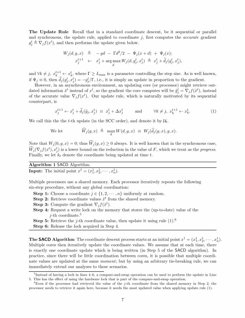
The Update Rule Recall that in a standard coordinate descent, be it sequential or paralleland synchronous, the update rule, applied to coordinate j, first computes the accurate gradientgtj , ∇jf(x

t), and then performs the update given below.

Wj(d, g, x) , − gd − Γd2/2 − Ψj(x+ d) + Ψj(x);

xt+1j ← xtj + argmax

dWj(d, g

tj , x

tj) , xtj + dj(g

tj , x

tj),

and ∀k 6= j, xt+1k ← xtk, where Γ ≥ Lmax is a parameter controlling the step size. As is well known,

if Ψj ≡ 0, then dj(gtj , x

tj) = −gtj/Γ, i.e., it is simply an update in proportion to the gradient.

However, in an asynchronous environment, an updating core (or processor) might retrieve out-dated information xt instead of xt, so the gradient the core computes will be gtj = ∇jf(x

t), insteadof the accurate value ∇jf(x

t). Our update rule, which is naturally motivated by its sequentialcounterpart, is

xt+1j ← xtj + dj(gj , x

tj) ≡ xtj +∆xtj and ∀k 6= j, xt+1

k ← xtk. (1)

We call this the the t-th update (in the SCC order), and denote it by Ut.

We let Wj(g, x) , maxd

W (d, g, x) ≡ Wj(dj(g, x), g, x).

Note that Wj(0, g, x) = 0; thus Wj(g, x) ≥ 0 always. It is well known that in the synchronous case,

Wj(∇jf(xt), xtj) is a lower bound on the reduction in the value of F , which we treat as the progress.

Finally, we let kt denote the coordinate being updated at time t.

Algorithm 1 SACD Algorithm.

Input: The initial point x1 = (x11, x12, · · · , x1n).

Multiple processors use a shared memory. Each processor iteratively repeats the followingsix-step procedure, without any global coordination:

Step 1: Choose a coordinate j ∈ {1, 2, · · · , n} uniformly at random.Step 2: Retrieve coordinate values xt from the shared memory.Step 3: Compute the gradient ∇jf(x

t).Step 4: Request a write lock on the memory that stores the (up-to-date) value of the

j-th coordinate.5

Step 5: Retrieve the j-th coordinate value, then update it using rule (1).6

Step 6: Release the lock acquired in Step 4.

The SACD Algorithm The coordinate descent process starts at an initial point x1 = (x11, x12, · · · , x1n).

Multiple cores then iteratively update the coordinate values. We assume that at each time, thereis exactly one coordinate update which is being written (in Step 5 of the SACD algorithm). Inpractice, since there will be little coordination between cores, it is possible that multiple coordi-nate values are updated at the same moment ; but by using an arbitrary tie-breaking rule, we canimmediately extend our analyses to these scenarios.

5Instead of having a lock in lines 4–6, a compare-and-swap operation can be used to perform the update in Line5. This has the effect of using the hardware lock that is part of the compare-and-swap operation.

6Even if the processor had retrieved the value of the j-th coordinate from the shared memory in Step 2, theprocessor needs to retrieve it again here, because it needs the most updated value when applying update rule (1).

7

In Algorithm 1, we provide the complete description of SACD. The retrieval times for Step 2 plusthe gradient-computation time for Step 3 can be non-trivial, and also in Step 4 a core might needto wait if the coordinate it wants to update is locked by another core. Thus, during this period oftime other coordinates are likely to be updated. For each update, we call the period of time spentperforming the six-step procedure the span of the update. We say that update A interferes withupdate B if the commit time of update A lies in the span of update B.

Later in this section, we discuss why locking is needed and when it can be avoided; we alsoexplain why the random choice of coordinate should be made before retrieving coordinate values.

Managing the Undoing of Uniformity: The Single Coordinate Consistent Order Beforestating our result formally, we need to disambiguate our timing scheme. In every asynchronousiterative system, including our SACD algorithm, each procedure runs over a span of time ratherthan atomically. Generally, these spans are not consistent — it is possible for one update to startlater than another one but to commit earlier. To create an analysis, we need a scheme that ordersthe updates in a consistent manner.

Using the commit times of the updates for the ordering seems the natural choice, since thisensures that future updates do not interfere with the current update. This is the choice made inmany prior works. However, as discussed by Mania et al. [20], this causes uniformity to be undone,as shown in the following example.

Example 1. Suppose there are three cores and four coordinates, suppose that the workload forupdating x1 is 2.99 time units, the workloads for updating x2, x3, x4 are 1 time unit (the 2.99 is toavoid ties), and suppose every update takes the same 0.5 time units for Steps 4–6. Assuming thecores all start at the same time, then P [k1 = 1] = 1/43, which is the probability that all cores chooseto update the first coordinate. Contrariwise, P [k2 = 1 | k1 = 1] = 1. And, in general, the probabilitydistribution which the random variable kt follows is strongly dependent on the recent history.

When there are many more cores and coordinates than the simple case we just considered, andwhen the other asynchronous effects7 are taken into account, it is highly uncertain what is the exactor even an approximate distribution for kt+1 conditioned on knowledge of the history of k1, · · · , kt.

To bypass the above issue, we introduce the Single Coordinate Consistent Order, SCC for short,defined as follows. We begin from the updates ordered by start time. Then, for each coordinateseparately, we rearrange the updates to this coordinate so that they are in commit order, whilecollectively occupying the same places in the start ordering. The next example illustrates all threeorders. The start times given by the ST order correspond to actual times; but henceforth, the indext will refer to the position of an update in the SCC order, and to the values computed by theseupdates.

Example 2. In Figure 1 we show six updates to two variables, x1 and x2, starting at times t = 1to 6, and ending at times 7–12. The updates are named U1–U6. In the order listings below, tofacilitate comparisons, we give each update an argument comprising the variable it updates.

Update Orders:

ST: U1(x2), U2(x1), U3(x1), U4(x2), U5(x1), U6(x2)

CT: U1(x2), U3(x1), U6(x2), U2(x1), U5(x1), U4(x2)

SCC: U1(x2), U3(x1), U2(x1), U6(x2), U5(x1), U4(x2)

The updates to x1 are in the same positions in the ST and SCC orders, in the same order in theCT and SCC orders. Likewise for x2.

8

t = 1

t = 2

t = 3

t = 4

t = 5

t = 6

t = 7

t = 8

t = 9

t = 10

t = 11

t = 12

U1

U2U3

U4U5 U6

updates to x1 updates to x2

Figure 1: Illustration of the ST, CT and SCC orders

We can also understand the SCC order in terms of start times 1, 2, . . . , T . The t-th update inthe ST order starts at time t and commits at some integer time in the range [t+ 1, t+ q + 1] (thisfollows from our assumption that the asynchrony is q-bounded). Remember that the “times” aresimply providing an ordering; they are not measured in a common unit. Ut, the t-th update in theSCC order, has an integer start time in the range [max{1, t− q + 1}, t+ q − 1] and commits at aninteger time in the range [t+ 1, t+ q + 1] (see Lemma 1).

Clearly the history has no influence on the choice of kt+1. However, there is a new issue: futureupdates can interfere with the current update. Here the term future is used w.r.t. the SCC order;recall that an update Ua to one coordinate with an earlier starting time can commit later thananother later starting update Ub to a different coordinate, and therefore Ub could interfere with Ua.

Further Remarks about the SACD Algorithm In many optimization problems, e.g., thoseinvolving sparse matrices, the number of coordinate values needed for computing the gradient inStep 3 of Algorithm 1 is much smaller than n, i.e., in Step 2, the core needs to retrieve only a tinyportion of the full set of coordinate values. Also, the sets of coordinate values needed for computingthe gradients along different coordinates can be very different. Therefore, the random choice ofcoordinate (in Step 1) should be made ahead of the process of retrieving required information fromthe shared memory.

If the convex function F does not have the univariate non-smooth components, each updatesimply adds a number, which depends only on the computed gradient, to the current value in thememory. Then the update can be done atomically (e.g., by fetch-and-add8), and no lock is required.

However, for general scenarios with univariate non-smooth components, the update to xj mustdepend on the value of xj in memory right before the update (see (1)). Then the update cannotbe done atomically, and a lock is necessary. We note that when the number of cores is far fewerthan n, say when it is ǫ

√n for some ǫ < 1, delays due to locking can occur, but are unlikely to be

7E.g., communication delays, interference from other computations (say due to mutual exclusion when multiplecores commit updates to the same coordinate), interference from the operating system and CPU scheduling.

8The fetch-and-add CPU instruction atomically increments the contents of a memory location by a specified value.

9

significant.9 As already mentioned, even if the update is carried out using a Compare-and-Swapoperation, the lock is still present within the hardware implementation of this operation.

Justifying the SCC Order We begin by justifying why Step 5 in the update algorithm needs touse the most up-to-date value of x1 (or more generally, of xj), via the the following convex functionexample.

Example 3. Let F be a convex function on n − 1 variables. Then define the n variable convexfunction F as follows.

F (x) =1

2x21 +Ψ1(x1) + F (x2, . . . , xn)

where Ψ1(x1) =

{0 if − 1 ≤ x1 ≤ 1

2∞ otherwise

Suppose Γ = 1, and suppose xt1 = −1. Further suppose the t-th and (t + 1)-st updates are both tox1, and suppose they both read the value xt1 for their gradient computation. Then they computeincrements argmax{d − d2/2 − Ψ(x1 + d) + Ψ(x1)}. If they both used the value −1 for x1 theywould both increment x1 by +1; the two updates would result in x1 being set to 1, a value for whichF =∞.

Note that update rule (1) implies that the sequence x1, x2, . . . , xT+1 is obtained by applyingthe computed increments ∆x1,∆x2, . . .∆xT , one at a time, and in this order. For this order tobe consistent with Step 5 using the most up-to-date value, we need that in this order, for eachindividual coordinate, the updates be in their up-to-date order, i.e. in their commit order. This iswhy we use the SCC order for our analysis. In the next example, we will show that an analysisbased on the ST order need not work when F has a non-smooth part Ψ.

Example 4. Let F be a convex function on n − 1 variables. Then define the n variable convexfunction F as follows.

F (x) =1

2x21 +Ψ1(x1) + F (x2, . . . , xn)

where Ψ1(x1) =

{0 if x1 ≥ −1∞ otherwise

Suppose Γ = 1, and suppose x01 = −1. Further suppose there are three consecutive updates to x1:

• Updates 1–3 start at times 1–3 respectively.

• At time 4, Updates 2 and 3 read the value of x1 (which equals −1) and calculate the gradientw.r.t. x1 (∇x1

f = −1).

• At times 5 and 6 respectively, Updates 2 and 3 apply the update on x1 (x′1 ← x1−argmaxd{ 1Γ∇x1

f ·d−Γd2/2−Ψ1(x1 + d)+Ψ1(x1)}). A simple calculation shows that both these updates incre-ments x1 by 1. Therefore, after time 6, the most up to date value of x1 is −1 + 1 + 1 = 1.

• At time 7, Update 1 reads the value of x1 (which now equals 1 after applying Updates 2 and3) and calculates the gradient w.r.t. x1 (∇x1

f = 1);

9The standard birthday paradox result states that if ǫ√

n cores each chooses a random coordinate among [n]uniformly, the probability of a collision is Θ(ǫ2).

10

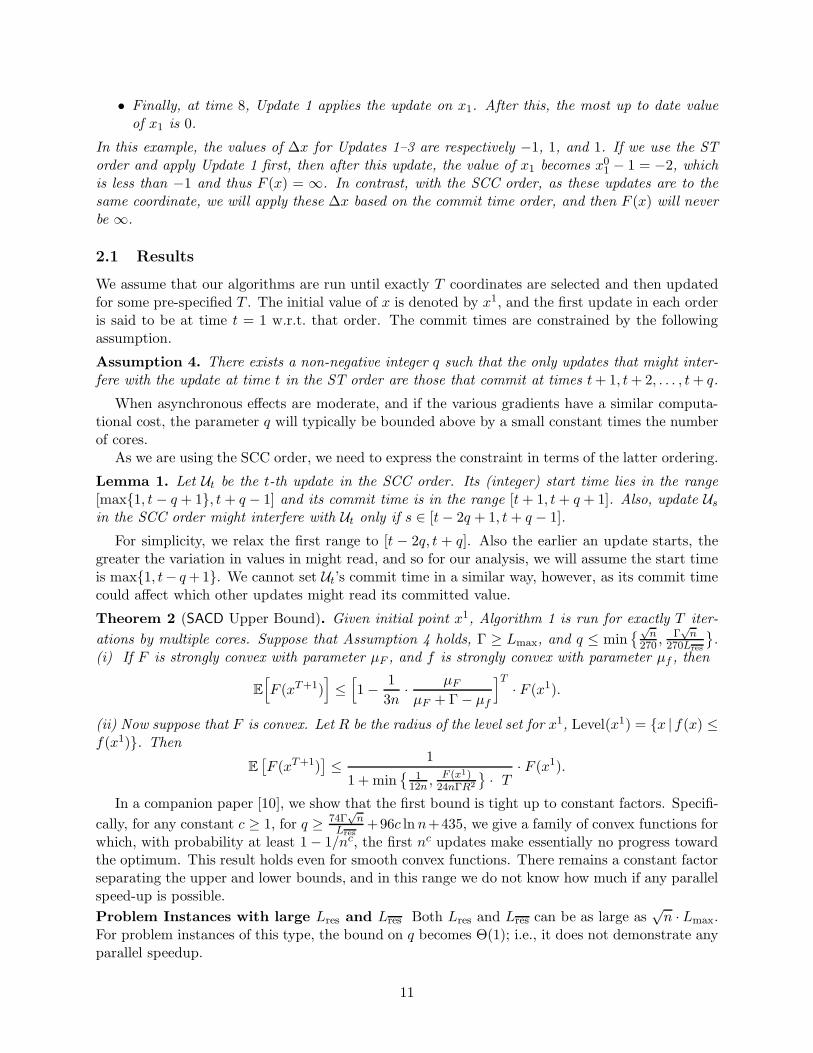
• Finally, at time 8, Update 1 applies the update on x1. After this, the most up to date valueof x1 is 0.

In this example, the values of ∆x for Updates 1–3 are respectively −1, 1, and 1. If we use the STorder and apply Update 1 first, then after this update, the value of x1 becomes x01 − 1 = −2, whichis less than −1 and thus F (x) = ∞. In contrast, with the SCC order, as these updates are to thesame coordinate, we will apply these ∆x based on the commit time order, and then F (x) will neverbe ∞.

2.1 Results

We assume that our algorithms are run until exactly T coordinates are selected and then updatedfor some pre-specified T . The initial value of x is denoted by x1, and the first update in each orderis said to be at time t = 1 w.r.t. that order. The commit times are constrained by the followingassumption.

Assumption 4. There exists a non-negative integer q such that the only updates that might inter-fere with the update at time t in the ST order are those that commit at times t+ 1, t+ 2, . . . , t+ q.

When asynchronous effects are moderate, and if the various gradients have a similar computa-tional cost, the parameter q will typically be bounded above by a small constant times the numberof cores.

As we are using the SCC order, we need to express the constraint in terms of the latter ordering.

Lemma 1. Let Ut be the t-th update in the SCC order. Its (integer) start time lies in the range[max{1, t− q + 1}, t+ q − 1] and its commit time is in the range [t+ 1, t+ q + 1]. Also, update Usin the SCC order might interfere with Ut only if s ∈ [t− 2q + 1, t+ q − 1].

For simplicity, we relax the first range to [t − 2q, t + q]. Also the earlier an update starts, thegreater the variation in values in might read, and so for our analysis, we will assume the start timeis max{1, t− q+1}. We cannot set Ut’s commit time in a similar way, however, as its commit timecould affect which other updates might read its committed value.

Theorem 2 (SACD Upper Bound). Given initial point x1, Algorithm 1 is run for exactly T iter-

ations by multiple cores. Suppose that Assumption 4 holds, Γ ≥ Lmax, and q ≤ min{√

n270 ,

Γ√n

270Lres

}.

(i) If F is strongly convex with parameter µF , and f is strongly convex with parameter µf , then

E

[F (xT+1)

]≤[1− 1

3n· µF

µF + Γ− µf

]T· F (x1).

(ii) Now suppose that F is convex. Let R be the radius of the level set for x1, Level(x1) = {x | f(x) ≤f(x1)}. Then

E[F (xT+1)

]≤ 1

1 + min{

112n ,

F (x1)24nΓR2

}· T· F (x1).

In a companion paper [10], we show that the first bound is tight up to constant factors. Specifi-

cally, for any constant c ≥ 1, for q ≥ 74Γ√n

Lres+96c ln n+435, we give a family of convex functions for

which, with probability at least 1− 1/nc, the first nc updates make essentially no progress towardthe optimum. This result holds even for smooth convex functions. There remains a constant factorseparating the upper and lower bounds, and in this range we do not know how much if any parallelspeed-up is possible.

Problem Instances with large Lres and Lres Both Lres and Lres can be as large as√n · Lmax.

For problem instances of this type, the bound on q becomes Θ(1); i.e., it does not demonstrate anyparallel speedup.

11

3 The Basic Framework

Recall that kt denotes the index of the coordinate that is updated at time t. We let gtkt := ∇ktf(xt)

denote the value of the gradient along coordinate kt computed at time t using up-to-date valuesof the coordinates, and gtkt denote the actual value computed, which may use some out-of-datecoordinate values.

3.1 Classical Analysis of Stochastic Sequential Coordinate Descent

This classical analysis proceeds by first showing that for any chosen kt, F (xt)−F (xt+1) ≥ Wkt(gtkt, xtkt).

Taking the expectation yields

E[F (xt)− F (xt+1)

]≥ 1

n

n∑

j=1

Wj(gtj , x

tj)

≥ 1

n· µF

µF + Γ− µf· F (xt) (by [25, Lemmas 4,6])

,α

n· F (xt). (2)

Note that in strongly convex case, we have defined α ,µF

µF+Γ−µf. It follows that E

[F (xt+1)

]≤

(1− αn ) · E

[F (xt)

]; iterating this inequality yields E

[F (xt+1)

]≤ (1− α

n )t · F (x1).

3.2 Warm-up: A Simple Analysis for the Strongly Convex Case with the Strong

Common Value Assumption

The following analysis already generalizes and improves the results shown in Liu et al. [18] and Liuand Wright [17].

Suppose there are a total of T updates. We view the whole stochastic process as a branchingtree of height T . Each node in the tree corresponds to the moment when some core randomly picksa coordinate to update, and each edge corresponds to a possible choice of coordinate. We use π todenote a path from the root down to some leaf of this tree. A superscript of π on a variable willdenote the instance of the variable on path π. Note that for each path π we reorder the coordinateinstances so that they are in the SCC order. For each path π and for each coordinate k, this simplyreorders the instances of xk on path π.

Contrary to intuition, in general we cannot associate a single value of x with each node of thetree because future choices of coordinate to update can affect the recent past; thus we need tospecify the path in order to know a coordinate value. In contrast, the SCV assumption ensuresthere is a single value of x for each node. A double superscript of (π, t) will denote the instance ofthe variable at time t on path π, i.e., right before the t-th update.

As we will be computing expected values by averaging over the n random coordinate choices forthe t-th update Ut, we introduce a notation to capture this choice: π(k, t) will denote the path withthe time t coordinate on path π replaced by coordinate k. Note that π(kt, t) = π. (Recall that ktis the coordinate chosen by update Ut on path π.)

Recall that xπ,t denotes the value of x on path π when precisely the first t − 1 updates in theSCC order have been applied; however, xπ,t may or may not actually be present in memory at anytime. Also, recall that xπ,t+1

kt= xπ,tkt

+ ∆xπ,tkt, and xπ,t+1

k = xπ,tk for k 6= kt, where ∆xπ,tktis the

increment computed by Ut. So xπ(k,t),tkt

denotes the value of xkt on path π(k, t) immediately prior

to update Ut, and xπ(k,t),sks

denotes the value of xks on path π(k, t) immediately prior to update Us.

12

Similarly, gπ,tkt, ∇ktf(x

π,t) denotes the true (accurate) gradient on path π immediately prior to

update Ut, gπ,tktthe inaccurate gradient used by Ut on path π, and g

π(k,t),tk the inaccurate gradient

used by Ut on path π(k, t).To handle the case where inaccurate gradients are used, we employ the following two lemmas.

Lemma 2. If Γ ≥ Lmax, F (xπ,t)− F (xπ,t+1) ≥ Wkt(gπ,tkt

, xπ,tkt)− 1

Γ · (gπ,tkt− gπ,tkt

)2.

Lemma 3. If Γ ≥ Lmax, F (xπ,t)−F (xπ,t+1) ≥ Γ4

(∆xπ,tkt

)2− 1

Γ ·(gπ,tkt− gπ,tkt

)2, where ∆xπ,tktdenotes

the increment computed by update Ut.

Proving these results for smooth functions is straightforward. The version for non-smoothfunctions is less simple, and makes use of the SCC order; it follows from Lemma 17 in Appendix A.

Combining Lemmas 2 and 3 yields

F (xπ,t)− F (xπ,t+1) ≥ 1

2· Wkt(g

π,tkt

, xπ,tkt) +

Γ

8

(∆xπ,tkt

)2− 1

Γ· (gπ,tkt

− gπ,tkt)2. (3)

As we will see, the following claim is one reason why this analysis, which uses the SCV assump-tion, is much simpler than that for the fully asynchronous setting.

Claim 1. With the SCV assumption, (i) for any τ ≤ t, xπ(k,t),τ is the same for any coordinate k,and thus equals xπ,τ ; (ii) for any τ ≤ t, xπ(k,t),τ is the same for any coordinate k, and thus equalsxπ,τ .

Proof. Part (i) follows directly from the SCV assumption.For part (ii), we argue inductively on τ as follows. Suppose the claim holds for earlier times.

By part (i), for any two coordinates k, k′, xπ(k′,t),τ−1 = xπ(k,t),τ−1 for τ ≤ t. Thus the computed

gradients for update Uτ−1 are the same on paths π(k′, t) and π(k, t). Also, as the claim holds forearlier times, the values read on both paths for Step 5 of update Uτ−1 are the same, meaning thatthese updates are identical and hence so are the outcome of these updates; i.e., xπ(k

′,t),τ = xπ(k,t),τ .As this is true for all τ ≤ t, the claim follows.

We take expectations over all paths π on both sides of inequality (3). We compute the ex-

pectation of 12 · Wkt(g

π,tkt

, xπ,tkt) as follows. We group each collection of n paths which differ only

on their t-th coordinate choice; in other words, if π is a path in a group, then the n paths inthe group are π(1, t), π(2, t), . . . , π(n, t). We first take the expectation within each group, which

is the summation 12n ·

∑nk=1 Wk(g

π(k,t),tk , x

π(k,t),tk ). By Claim 1(ii), xπ(k,t),t = xπ,t for any coordi-

nate k, and hence gπ(k,t),tk = ∇kf(x

π(k,t),t) = ∇kf(xπ,t) = gπ,tk . Thus the summation simplifies to

12n ·∑n

k=1 Wk(gπ,tk , xπ,tk ), which is at least α

2n ·F (xπ,t) by inequality (2). Then we take the expectationover all groups to obtain

E[F (xπ,t+1)

]≤(1− α

2n

)· E[F (xπ,t)

]

− E

[Γ8·(∆xπ,tkt

)2− 1

Γ· (gπ,tkt

− gπ,tkt)2]. (4)

To obtain E[F (xT+1)

]≤(1− α

2n

)T · F (x1), it suffices to show that

T∑

t=1

Γ

8· E[(

∆xπ,tkt

)2](1− α

2n

)T−t≥

T∑

t=1

1

Γ· E[(gπ,tkt

− gπ,tkt)2] (

1− α

2n

)T−t. (5)

13

In the remainder of this section we give a simple proof of the above inequality. We first proveLemma 4 below, which bounds the expectation, within each group of n paths, of the gradientdifferences squared.

Lemma 4. With the Strong Common Value assumption,

Ek[(gπ(k,t),tk − g

π(k,t),tk )2] ≤ 3qL2

res

n

∑

s∈[t−2q,t+q]\{t}Ek[(∆x

π(k,t),sks

)2].

Proof. By definition, gπ(k,t),tk = ∇kf(x

π(k,t),t), the gradient of up-to-date point xπ(k,t),t, and gπ(k,t),tk =

∇kf(xπ(k,t),t), the gradient of the point actually read from main memory, out-of-date point xπ(k,t),t.

By Lemma 1, the updates Us, for s < t − 2q, have been written into memory before update Utstarts. Thus, the difference between xπ(k,t),t and xπ(k,t),t is due to a subset U of the updates Uswith s ∈ [t− 2q, t+ q] \ {t}. Let

U = {t1, t2, ..., t|U |}.

Viewing ∆xπ(k,t),tikti

as the n-vector with a non-zero entry for coordinate kti and zero elsewhere,

we have:

xπ(k,t),t = xπ(k,t),t +

|U |∑

i=1

{∆x

π(k,t),tikti

if ti < t;

−∆xπ(k,t),tikti

if ti > t.

We define: xπ(k,t),t[j] = xπ(k,t),t +

j∑

i=1

{∆x

π(k,t),tikti

if ti < t;

−∆xπ(k,t),tikti

if ti > t.

Then, xπ(k,t),t[0] = xπ(k,t),t and xπ(k,t),t[|U |] = xπ(k,t),t. By the definition of Lres and the triangleinequality, we obtain

∥∥∥∇f(xπ(k,t),t)−∇f(xπ(k,t),t)∥∥∥2

≤( |U |−1∑

j=0

∥∥∥∇f(xπ(k,t),t[j + 1])−∇f(xπ(k,t),t[j])∥∥∥)2

≤( |U |∑

i=1

Lres

∣∣∣∆xπ(k,t),tikti

∣∣∣)2

≤ 3q∑

s∈[t−2q,t+q]\{t}L2res

(∆x

π(k,t),sks

)2. (6)

The last inequality followed from applying the Cauchy-Schwarz inequality to the RHS, andrelaxing U to [t− 2q, t+ q] \ {t}.

By Claim 1(i), xπ(k′,t),t = xπ(k,t),t. By Claim 1(ii), xπ(k

′,t),t = xπ(k,t),t. Thus,

14

Ek

[(g

π(k,t),tk − g

π(k,t),tk )2

]= Ek

[|∇kf(x

π(k,t),t)−∇kf(xπ(k,t),t)|2

]

=1

n

∑

k′

|∇k′f(xπ(k′,t),t)−∇k′f(x

π(k′,t),t)|2

=1

n

∑

k′

|∇k′f(xπ(k,t),t)−∇k′f(x

π(k,t),t)|2

=1

n· ‖∇f(xπ(k,t),t)−∇f(xπ(k,t),t)‖2

≤ 3qL2res

n

∑

s∈[t−2q,t+q]\{t}(∆x

π(k,t),sks

)2 (by 6). (7)

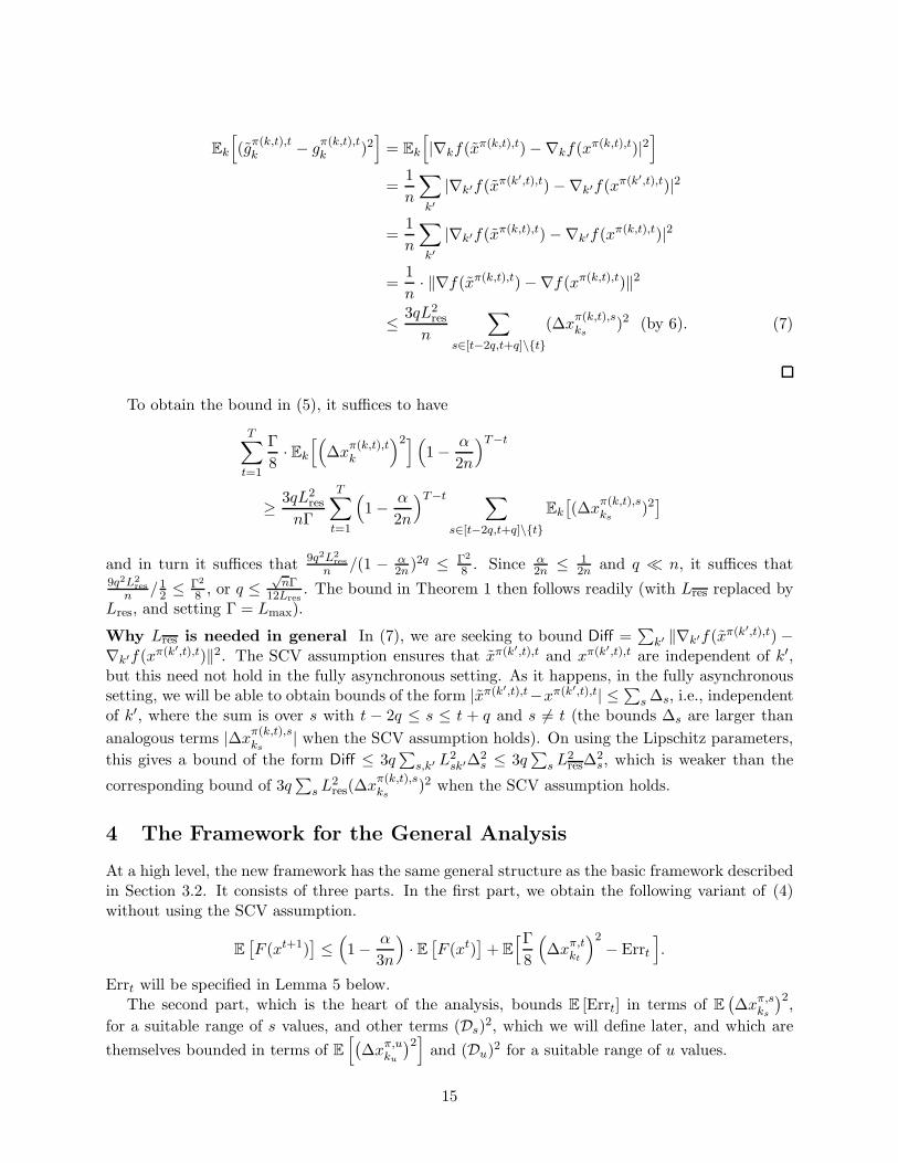
To obtain the bound in (5), it suffices to have

T∑

t=1

Γ

8· Ek

[(∆x

π(k,t),tk

)2] (1− α

2n

)T−t

≥ 3qL2res

nΓ

T∑

t=1

(1− α

2n

)T−t ∑

s∈[t−2q,t+q]\{t}Ek

[(∆x

π(k,t),sks

)2]

and in turn it suffices that 9q2L2res

n /(1 − α2n)

2q ≤ Γ2

8 . Since α2n ≤ 1

2n and q ≪ n, it suffices that9q2L2

res

n /12 ≤ Γ2

8 , or q ≤√nΓ

12Lres. The bound in Theorem 1 then follows readily (with Lres replaced by

Lres, and setting Γ = Lmax).

Why Lres is needed in general In (7), we are seeking to bound Diff =∑

k′ ‖∇k′f(xπ(k′,t),t) −

∇k′f(xπ(k′,t),t)‖2. The SCV assumption ensures that xπ(k

′,t),t and xπ(k′,t),t are independent of k′,

but this need not hold in the fully asynchronous setting. As it happens, in the fully asynchronoussetting, we will be able to obtain bounds of the form |xπ(k′,t),t−xπ(k

′,t),t| ≤∑s∆s, i.e., independentof k′, where the sum is over s with t − 2q ≤ s ≤ t + q and s 6= t (the bounds ∆s are larger than

analogous terms |∆xπ(k,t),sks

| when the SCV assumption holds). On using the Lipschitz parameters,

this gives a bound of the form Diff ≤ 3q∑

s,k′ L2sk′∆

2s ≤ 3q

∑s L

2res∆

2s, which is weaker than the

corresponding bound of 3q∑

s L2res(∆x

π(k,t),sks

)2 when the SCV assumption holds.

4 The Framework for the General Analysis

At a high level, the new framework has the same general structure as the basic framework describedin Section 3.2. It consists of three parts. In the first part, we obtain the following variant of (4)without using the SCV assumption.

E[F (xt+1)

]≤(1− α

3n

)· E[F (xt)

]+ E

[Γ8

(∆xπ,tkt

)2− Errt

].

Errt will be specified in Lemma 5 below.The second part, which is the heart of the analysis, bounds E [Errt] in terms of E

(∆xπ,sks

)2,

for a suitable range of s values, and other terms (Ds)2, which we will define later, and which are

themselves bounded in terms of E[(∆xπ,uku

)2]and (Du)

2 for a suitable range of u values.

15

The third part deduces the bounds in Theorem 2, by means of a suitable potential function(a.k.a. a Lyapunov function) and an amortized analysis.

4.1 Part 1: Demonstrating Substantial Progress

Recall that π(k, t) denotes the path in which coordinate kt at time t is replaced by coordinate k; toreduce clutter we now abbreviate this as π(k). Note that π(kt) = π. We let prev(t, k) denote thetime of the most recent update to coordinate k, if any, in the time range [t− 2q, t− 1]; otherwise,we set it to t.

Lemma 5.

E[F (xt)− F (xt+1)

]

≥ 1

3n2E

[ n∑

k=1

n∑

kt=1

Wk(gπ(kt),tk , x

π(kt),tk )

]+ E

[Γ8

(∆xπ,tkt

)2− Errt

],

where Errt =1

3n2

[ ∑

t−2q≤s<t&s=prev(t,ks)

n∑

kt=1

(3

2Γ

(gπ(kt),sks

− gπ(kt),tks

)2︸ ︷︷ ︸

A

+ 2Γ(xπ(ks),tks

− xπ(kt),tks

)2︸ ︷︷ ︸

B

+3Γ

2

(∆x

π(kt),sks

)2︸ ︷︷ ︸

C

)]

+1

n2

n∑

k=1

n∑

kt=1

2

3Γ

(gπ(k),tk − g

π(kt),tk

)2

︸ ︷︷ ︸D

+1

Γ

(gπ,tkt− gπ,tkt

)2

︸ ︷︷ ︸E

.

By (2),

n∑

k=1

n∑

kt=1

Wk(gπ(kt),tk , x

π(kt),tk ) ≥

n∑

kt=1

αF (xπ(kt),t),

which gives E[F (xt+1)

]≤(1− α

3n

)E[F (xt)

]+ E

[Γ8

(∆xπ,tkt

)2− Errt

].

To prove Lemma 5, we start from (3), and then apply the following two lemmas regarding

shifting the parameters in W . (See Appendix A for proofs.)

Lemma 6 (W Shifting on the g parameter). For any gj , g′j ,

Wj(gj , xj) ≥2

3· Wj(g

′j , xj) −

4

3Γ· (gj − g′j)

2.

Lemma 7 (W Shifting on the x parameter). Suppose there are ℓ updates to coordinate k over thetime interval [t− 2q, t− 1]. Then

if ℓ = 0, W (gπ,tk , xπ(k),tk ) = W (gπ,tk , xπ,tk )

if ℓ > 0, W (gπ,tk , xπ(k),tk ) ≥ W (gπ,tk , xπ,tk )− 3

2Γ· (gπ,prev(t,k)k − gπ,tk )2

− 2Γ(xπ,tk − xπ(k),tk )2 − 3Γ

2· (∆x

π,prev(t,k)k )2.

16

4.2 Part 2: Bounding Errt, the Error Term

We begin by stating the following lemma, which bounds the difference in the increments computedby two updates to a coordinate xj when the inputs to Step 5 vary. To avoid notational clutter, we

write Ψ and d in lieu of Ψj and dj (to review its definition see the update rule in Section 2); also,by x1 and x2 we mean two possible values of xj, and by g1 and g2 two possible values of gj .

Lemma 8. For any g1, g2, x1, x2 ∈ R and Γ ∈ R+, |d(g1, x1)− d(g2, x2)| ≤ |x1 − x2|+ 1

Γ · |g1 − g2|,and hence (

d(g1, x1)− d(g2, x2))2≤ 2(x1 − x2)

2 +2

Γ2· (g1 − g2)

2 .

If Ψ is the zero function, then |d(g1, x1)− d(g2, x2)| = 1Γ · |g1 − g2|.

4.2.1 Additional Notation

In this subsection, we will be defining notation of the form ƥmaxx

π,sks

, where • refers to variousparameters we will specify as needed, and the max refers to taking a suitable maximum. Withoutspelling it out, we will assume the analogous notation with ∆•

min is also being defined. In addi-tion, we will define ƥ

spanxπ,sks

, ƥmaxx

π,sks−∆•

minxπ,sks

, and ƥvarx

π,sks

, max{|ƥminx

π,sks|, |∆•

maxxπ,sks|,

ƥspanx

π,sks}.

The next step in our analysis is to generalize Lemma 4 to settings in which the SCV Assumptionneeds not hold, so as to bound the “error” terms in Errt. We seek to carry out an analysis analogousto (7). The first difficulty we face is that the bound we obtain is going to depend on the span ofpossible values of ∆xπ,sks

, which we denote by ∆spanxπ,sks

, where ∆maxxπ,sks

is the maximum possiblevalue for this increment over all asynchronous schedules on path π, assuming the first t − 2q − 1updates are already fixed. Thus, in addition to bounds on the various gradient differences, we willneed to bound ∆spanx

π,sks

. We begin with this task.Notice that we have assumed that the first t − 2q − 1 updates are known rather than the first

s − 2q − 1. To reflect this, we denote the maximum possible value of the update by ∆tmaxx

π,sks

,and analogously, we write ∆t

spanxπ,sks

. We are interested in (s, t) pairs with t − 2q ≤ s ≤ t + q, orequivalently, s − q ≤ t ≤ s + 2q; these are the updates Us whose value may not be determined atthe start of update Ut and which may affect update Ut. We call t the reference time for update Us.

For notational convenience, rather than give a bound on ∆tspanx

π,sks

, we will bound ∆uspanx

π,tkt

instead. So, suppose that the first u − 2q − 1 updates have been fixed, for some u with t − q ≤u ≤ t+ 2q. Let xπ,u,tmax,kt

and xπ,u,tmin,kt, resp., be the largest and smallest values that xπ,tkt

could attain

with the first u− 2q − 1 updates already fixed; similarly, let gπ,u,tmax,ktand gπ,u,tmin,kt

be the largest andsmallest gradient values that could be computed by update Ut with the first u − 2q − 1 updatesalready fixed.

Lemma 8 implies

(∆u

spanxπ,tkt

)2≤ 2(xπ,u,tmax,kt

− xπ,u,tmin,kt

)2+

2

Γ2

(gπ,u,tmax,kt

− gπ,u,tmin,kt

)2.

We use a Lipschitz bound to obtain

(gπ,u,tmax,kt

− gπ,u,tmin,kt

)2 ≤[ ∑

t−2q≤s≤t+qand s 6=t

Lkskt max{∣∣∆u

maxxπ,sks

∣∣,∣∣∆u

minxπ,sks

∣∣,

∆uspanx

π,sks

}]2.

17

The reason for the three terms is that in determining each gradient, for each s in the given range,the relevant update could be read or not read; so the difference due to this coordinate could stemfrom its maximum value, its minimum value, or their difference.

By the Cauchy-Schwartz inequality,

(∆u

spanxπ,tkt

)2≤ 2(xπ,u,tmax,kt

− xπ,u,tmin,kt

)2

+6q

Γ2

∑

t−2q≤s≤t+qand s 6=t

L2kskt max

{∣∣∆umaxx

π,sks

∣∣2,∣∣∆u

minxπ,sks

∣∣2,(∆u

spanxπ,sks

)2}. (8)

Legitimate Averaging via Exclusion Recall that in Section 3.2, a crucial step for obtaining agood parallelism bound was to perform averaging over the n paths in each group, i.e., to replace theterms L2

ksktby L2

res by averaging over kt. To do this here we would need ∆umaxx

π,sks

and ∆uminx

π,sks

tohave the same value on every path π(k). But this need not be the case, because the computation of∆u

maxxπ,sks

could read the result of update Ut, and therefore depend on the choice of kt. To addressthis, we will create terms which upper bound ∆u

maxxπ,sks

and which have the same value on everypath π(k), and similarly for ∆u

minxπ,sks

.Our first key observation, concerns Us and Ut: one of them commits first. Suppose Us commits

first; then the value computed by Us does not use the value computed by Ut, either directly as aninput, or indirectly because its inputs do not use this value either. Otherwise, Us has no impact on∆u

spanxπ,tkt

.We introduce new terminology to capture this observation. If update Us commits before Ut, we

will say that Ut is excluded from the computation of Us. To capture the exclusion of Ut, we define

∆u,{t}max xπ,sks

to be the maximum value Us can compute on path π, assuming that Us commits beforeUt, and the first u− 2q − 1 updates are fixed.

The updates that cause the output of Us to vary are those that might commit before or afterUs; these are always a subset of the Uv with v ∈ [s − 2q, s + q]. We also observe that if update Uscommits before Ut, then Us commits before any update Uv with v > t+q. We can safely incorporate

this constraint in the notation ∆umax and ∆

u,{t}max . The notation extends to ∆span and ∆var in the

natural way.Note that π(k) and π(k′) are identical paths apart from the coordinate chosen at time t. The

phrase “Ut is excluded from the computation of Us” could cause us to conjecture that ∆u,{t}max x

π(k),sks

are identical for all k, and similarly for the ∆u,{t}min x

π(k),sks

. If it were so, we could rewrite (8) asfollows, and average over kt:

(∆u

spanxπ,tkt

)2≤ . . . +

6q

Γ2

∑

t−2q≤s≤t+qand s 6=t

L2res ·max

{. . . ,

(∆

u,{t}span x

π,sks

)2}.

However, this conjecture needs not be true with the current definition, so the above averaging isnot yet valid. For, as explained in the next paragraph, a problem can arise if there is a coordinatekv = kt with t < v ≤ t+ q; when averaging over all kt we are certain to encounter paths with thisproperty. (As an aside, we note that the conjecture is true when Ψ ≡ 0 and the ST order is used.)

Suppose kv = kt, v 6= t, and suppose Ut is excluded. Given the SCC order, it would appear Uvshould also be excluded. But then suppose there is some other update Us with t− 2q ≤ s ≤ t+ q,

ks 6= kt, and on some path π(k) where k 6= kt, in computing ∆u,{t}max xπ,sks

, Us reads the result of

18

update Uv. Then to be sure the same maximum value were computed by Us on path π, we wouldneed it to read this excluded value. So this value cannot be excluded. Instead, we define thecomputation to act as if it were in the SCC order, but with update Ut simply not present, i.e., asif there were a total of T − 1 updates over the whole computation. (This only pertains to updatesUs with t− 2q ≤ s ≤ t+ q and s 6= t.)

This looks promising, as we would anticipate that ∆u,{t}max xπ,sks

≤ ∆umaxx

π,sks

, and so it would seemthe last term on the RHS can be bounded recursively. But unfortunately, this property need nothold if there are updates to the same coordinate on π in the range [t + 1,min{s, u} + q]. Tounderstand the issue we revisit Example 3. Suppose updates Ut and Ut+1 are both to coordinatex1, with xt1 = −1 as before. If both updates are present, and both read value x1 = −1 for theirgradient computation, then Ut computes an increment of 1 and Ut+1 an increment of 1

2 . However,

if Ut is excluded, then Ut+1 computes an increment of 1; i.e., ∆u,{t}max xπ,t+1

kt+1> ∆u

maxxπ,t+1kt+1

, contraryto the desired property.

To avoid the difficulty illustrated by the above example, we will need to modify the definition

of ∆u,{t}max xπ,sks

. These modifications enable Lemma 9 below, which ensures ∆u,{t}max xπ,sks

has the prop-erties we need to carry out the averaging in the analysis. Recall that depending on the choiceof asynchronous schedule, Us may or may not read values computed by updates in the range[s− 2q,min{s, u}+ q] \ {t}. We will want to pretend that Us can make this choice for an expandedrange of updates, namely a subset of [s − 4q,min{s, u} + q] \ {t}. In effect, this enlarges the setof possible asynchronous schedules. To be very precise: let l be the maximum commit time forupdates U1,U2, . . . ,Uu−4q−1; Us may read or not read any values computed by updates Ur thatcommit after time l for r ∈ [s− 4q,min{s, u} + q] \ {t}. We call this Ur’s extended computation.

So as to identify the updates Ur with r ≥ u − 4q that commit by time l, we introduce thefollowing set Aπ,u of updates: Aπ,u = {r |u − 4q ≤ r < u − 2q and Ur has committed beforesome Up for p < u − 4q}, which means the updates in Aπ,u have committed before Uu startsits extended computation. Also, rather than just excluding Ut, we allow any additional subsetS = {v |u− 4q ≤ v ≤ u+ q}\Aπ,u of updates to be excluded; we follow this by maximizing over allsuch S. This also implies that the range of s in which we are interested becomes u−4q ≤ s ≤ u+q.

Note that if s ∈ Aπ,u then ∆u,{t}span x

π,sks

= 0.Later on, we will be allowing the exclusion of sets R other than just {t}, so we also incorporate

this in our definitions. For R,S disjoint from Aπ,u, we define:

∆u,R,Smax xπ,sks

,

the maximum value that ∆xπ,skscan assume when the

first (u− 4q − 1) updates and all updates in Aπ,u onpath π have been fixed, and update Uv is excludedfrom the computation of Us for v ∈ R ∪ S and forv > u+ q;

∆u,Rmaxx

π,sks

, maxS⊆[u−4q,u+q]\Aπ,u∪{s}∆u,R,Smax xπ,sks

.

∆umaxx

π,sks

, ∆u,∅maxx

π,sks

Now we have the desired properties:

Lemma 9. i. If t ∈ R and u ≤ t+ 2q, then ∆u,Rmaxx

π(k),sks

is identical on every path π(k).

ii. If s ≤ t then ∆t,Rmaxx

π,sks≤ ∆s,R

maxxπ,sks

.

iii. If R ⊂ R′ then ∆u,R′

maxxπ,sks≤ ∆u,R

maxxπ,sks

.

iv. ∆u,Rmaxx

π,sks≤ ∆u,∅

maxxπ,sks

.

19

Proof. i. We begin by showing that the set Aπ(k),u is the same for all k. Recall that u ≤ t + 2q.By Lemma 1, the start time for Ut is at least t − q + 1 ≥ u − 3q + 1. For p < u − 4q, again byLemma 1, Up has commit time at most u− 4q − 1+ q+1 = u− 3q. So if Ur commits before Up forsome p ≤ u− 4q, Ur has commit time at most u− 3q − 1. Thus Ur’s commit time is unaffected bythe choice of coordinate by Ut, and therefore Aπ(k),u is the same for all k.

Now, recall that π(k) is the path in which coordinate kt at time t on path π is replaced bycoordinate k. By definition, if t ∈ R, then Ut is excluded from the computation of ∆u,R

maxxπ,sks

. As

the paths π(k) are identical apart from their t-th coordinate, and as the sets Aπ(k),u are the same

for all these paths, it follows that ∆u,Rmaxx

π(k),sks

is exactly the same for every k.ii. This follows from the next two observations: (a) the update does not read any of the variable

values computed by updates Uv for v > s + q and therefore reducing the top end of the rangein going from reference time t to s does not change the possible updates computed by Us; (b)Aπ,s∩ [t−4q, t−2q) ⊆ Aπ,t, and therefore there are at least as many updates that are not yet fixedwith reference time s compared to reference time t; furthermore, the fixed values in Aπ,t \Aπ,s areall values that could be computed in the computation with reference time s.

iii. Recall the definition of ∆u,Rmaxx

π,sks

, and let S′ be the set for which ∆u,R′

maxxπ,sks

= ∆u,R′,S′

max xπ,sks.

Now, we let S = (R′∪S′) \R; thus S ∪R = S′∪R′. Clearly, ∆u,R′,S′

max xπ,sks= ∆u,R,S

max xπ,sks≤ ∆u,R

maxxπ,sks

.iv. This follows immediately from iii.

Recall that we defined ∆u,Rspanx

π,sks

= ∆u,Rmaxx

π,sks−∆u,R

minxπ,sks

and ∆u,Rvar x

π,sks

= max{∣∣∆u,R

maxxπ,sks

∣∣,∣∣∆u,R

minxπ,sks

∣∣,∆u,Rspanx

π,sks

}.

We want to have one term to cover every update in which xπ,sksis involved. Accordingly, we define

∆Rmaxx

π,sks

:= maxu:u−4q≤s

≤u+q

∆u,Rmaxx

π,sks

= maxu:s−q≤u

≤s+4q

∆u,Rmaxx

π,sks

= maxs−q≤u≤s

∆u,Rmaxx

π,sks

,

where we use Lemma 9(ii) for the final equality.

We let ∆u,Rspanx

π,sks

= ∆u,Rmaxx

π,sks− ∆u,R

minxπ,sks

, ∆Rspanx

π,sks

= ∆Rmaxx

π,sks− ∆

Rminx

π,sks

and ∆Rvarx

π,sks

=

max{∣∣∆R

maxxπ,sks

∣∣,∣∣∆R

minxπ,sks

∣∣,∆Rspanx

π,sks

}. We simplify the notation whenR = ∅, defining ∆maxx

π,sks

,

∆∅maxx

π,sks

, ∆spanxπ,sks

, ∆∅spanx

π,sks

and ∆varxπ,sks

, ∆∅varx

π,sks

. Clearly, if u ⊆ [s− q, s], then

∆u,Rspanx

π,sks≤ ∆

Rspanx

π,sks≤ ∆spanx

π,sks

and ∆u,Rvar x

π,sks≤ ∆

Rvarx

π,sks≤ ∆varx

π,sks

. (9)

Finally, we will want to know the expected effect of update Ut. Thus, we define

(Dt)2

, E

[(∆maxx

π,tkt−∆minx

π,tkt

)2]and

(∆X

t

)2, E

[(∆xπ,tkt

)2].

Since exactly T updates are made, we assume that (Dt)2 ,(∆X

t

)2 ≡ 0 for t = 0 and t ≥ T + 1throughout the analysis.

Next, we introduce analogous notation for the gradients.

20

gu,R,S,π,smax,ks

,

the maximum value of gπ,skscan assume when the

first (u− 4q − 1) updates on path π have been fixed, andupdate Uv is excluded from the computation of Us forv ∈ R ∪ S and for v > u+ q; for all r ∈ Aπ,u, thevalue of the update Ur is already fixed;

gu,R,π,smax,ks

, maxS⊆[u−4q,u+q]}\Aπ,u∪{s} gu,R,S,π,smax,ks

;

gR,π,smax,ks

, maxs−q≤u≤s gu,R,π,smax,ks

;

gπ,smax,ks, g∅,π,smax,ks

and gπ,sspan,ks

, gπ,smax,ks− gπ,smin,ks

.

4.2.2 Bounding (Dt)2 = E

[(∆spanx

π,tkt

)2 ]

We are now ready to bound (Dt)2. Let ν1 :=

20q2

n and ν2 =24q2L2

res

nΓ2 .

Lemma 10.

Γ · (Dt)2 ≤

(ν1q

+ν2q

)Γ

∑

s∈[t−5q,t+q]\{t}

[(Ds

)2+(∆X

s

)2 ].

Proof. Recall that ∆spanxπ,tkt

= maxt−q≤r≤t∆rmaxx

π,tkt−mint−q≤r′≤t∆

r′minx

π,tkt

. We call r and r′ thereference parameters. By Lemma 8, we obtain a bound of

maxt−q≤r,r′≤t

[2(xr,π,tkt

− xr′,π,t

kt

)2+

2

Γ2·(gr,∅,π,tkt

− gr′,∅,π,t

kt

)2], (10)

where xr,π,tktis the value of xπ,tkt

right before Step 5 of update Ut when r is the reference parameter;the maximum is also over the maximum and minimum possible values of the four terms in theabove expression.

The first difference on the RHS of the above expression is going to involve updates to coordinatexkt , i.e., updates Uks with ks = kt and min{r− 4q, r′− 4q} ≤ s < t. We will consider the maximum

and minimum possible values for these updates. This suggests a bound of(∆r

maxxπ,sks−∆r′

minxπ,sks

)2for each such s. But recall that the definition of ∆r

maxxπ,sks

allows the exclusion of updates Uv for aworst case set of v when computing Us (this is the effect of the maximization over S in the definition

of ∆rmax), and therefore the first difference in (10) may be as large as

(∆r

maxxπ,sks

)2or(∆r′

minxπ,sks

)2,

meaning that the actual bound is(max

{∣∣∆rmaxx

π,sks

∣∣,∣∣∆r′

minxπ,sks

∣∣, ∆rmaxx

π,sks−∆r′

minxπ,sks

})2.

By Lemma 9(ii), we can modify the range of r, r′ from [t− q, t] to [min{s, t− q}, s] ⊂ [s − q, s]as s < t. Thus the first term in (10) is bounded by

( ∑

t−5q≤s<tks=kt

∆{t}varx

π,sks

)2.

We use a similar argument to bound the second term in (10). The value of gr,∅,π,tktcan vary due

to the updates ∆rxπ,sksfor r− 4q ≤ s ≤ r+ q and s 6= t; equivalently, s− q ≤ r ≤ s+4q. Recall also

that t− q ≤ r ≤ t. Thus, for s > t, the relevant range of r is [s − q, t] ⊂ [s − q, s], and for s < t,as before, the relevant range is also at most [s− q, s]. Using the Lipschitz bound for the gradients,we obtain:

maxt−q≤r,r′≤t

(gr,∅,π,tkt

− gr′,∅,π,t

kt

)2 ≤( ∑

t−5q≤s≤t+qs 6=t

Lkskt∆{t}varx

π,sks

)2. (11)

21

Thus, using the Cauchy-Schwartz inequality for the second inequality below, we obtain

(∆spanx

π,tkt

)2≤ 2( ∑

t−5q≤s<tks=kt

∆{t}varx

π,sks

)2+

2

Γ2

( ∑

t−5q≤s≤t+qs 6=t

Lkskt∆{t}varx

π,sks

)2

≤ 10q∑

t−5q≤s<tks=kt

(∆

{t}varx

π,sks

)2+

12q

Γ2

∑

t−5q≤s≤t+qs 6=t

L2kskt

(∆

{t}varx

π,sks

)2.

Now we average over all n choices of kt; consequently, π is now being viewed as a random variablewhere kt on π is being chosen uniformly at random, while the coordinates at times other than t are

fixed. Notice that on all the paths π being considered in the averaging, the value of each ∆r,{t}max x

π,sks

is the same as their computation does not involve the update to xtkt, and because at most the first(t − 4q) updates have been fixed in any of these terms, none of the updates that could affect the

update to xtkt in its extended computation have been fixed; similarly for ∆r,{t}min xπ,sks

. Consequently,

for each s, the term ∆varxksπ,s is the same on each path. Thus the averaging is simply averaging the

values Lkskt as kt varies. Recall that by Definition 1, L2res = maxk

∑nj=1(Lkj)

2; this yields

Ekt

[ (∆spanx

π,tkt

)2 ]

≤ 10q

n

∑

t−5q≤s<t

(∆

{t}varx

π,sks

)2+

12q

nΓ2

∑

t−5q≤s≤t+qs 6=t

L2res ·

(∆

{t}varx

π,sks

)2

≤ 10q

n

∑

t−5q≤s<t

(∆varx

π,sks

)2+

12q

nΓ2

∑

t−5q≤s≤t+qs 6=t

L2res ·

(∆varx

π,sks

)2(by (9)). (12)

Now, ∆xπ,sks∈[∆s

minxπ,sks

, ∆smaxx

π,sks

]⊆[∆minx

π,sks

, ∆maxxπ,sks

]; thus,∣∣∆minx

π,sks

∣∣,∣∣∆maxx

π,sks

∣∣ ≤∣∣∆xπ,sks

∣∣ +(∆spanx

π,sks

). Also,

(∆minx

π,sks

)2,(

∆maxxπ,sks

)2 ≤ 2(∆xπ,sks

)2+ 2

(∆spanx

π,sks

)2. So,

(∆varx

π,sks

)2 ≤ 2(∆xπ,sks

)2

+ 2(∆spanx

π,sks

)2. Consequently,

Ekt

[ (∆spanx

π,tkt

)2 ]≤ Ekt

[20q

n

∑

t−5q≤s<t

(∆spanx

π,sks

)2+(∆xπ,sks

)2

+24qL2

res

nΓ2

∑

t−5q≤s≤t+qs 6=t

(∆spanx

π,sks

)2+(∆xπ,sks

)2].

Taking the expectation over every group, which on the RHS amounts to taking the expectationover every path π, yields

(Dt)2 = E

[(∆spanx

π,tkt

)2]≤ 20q

n

∑

t−5q≤s≤t

(E

[(∆spanx

π,sks

)2]+ E

[(∆xπ,sks

)2])

+24qL2

res

nΓ2

∑

t−5q≤s≤t+qs 6=t

(E

[(∆spanx

π,sks

)2]+ E

[(∆xπ,sks

)2]).

Lemma 10 follows.

22

4.2.3 Gradient Bounds

In the previous subsection, one of the terms being bounded was (gr,∅,π,tkt− gr

′,∅,π,tkt

)2 = (gπ,tmax,kt−

gπ,tmin,kt)2.

Here, we will bound term E,(gπ,tkt− gπ,tkt

)2. Unfortunately, gπ,tkt

might not be in[gπ,tmin,kt

, gπ,tmax,kt

]

and so we cannot simply apply Lemma 10. The reason is that gπ,tktis a function of xπ(kt),t, and this

up-to-date x value could depend on the value of update Ut; for recall that Ut might finish beforesome updates Us with s < t, and the latter updates could then read the updated value of thecoordinate being updated by Ut. As already explained, there are also other ways that the choice ofkt by update Ut could affect earlier updates.

We start by upper bounding term E by(∑

l0∈[t−2q,t−1] Lkl0 ,kt∆t,∅

varxπ,l0kl0

)2. The challenge is that

changing either coordinate kl0 or kt may change the value of ∆t,∅maxx

π,l0kl0

or of ∆t,∅minx

π,l0kl0

which implies

that a simple averaging of the terms L2kl0 ,kt

to obtain a term L2res as was done to obtain (12) is

not possible. Instead, we will bound this term recursively. The somewhat more general resultwe will need is stated in the following lemma. Its proof, which is quite involved, is deferred toAppendix A.4.

Let Λ2 =L2res

Γ2 + 1, r = 160q2Λ2

n , ν3 =316(

r2

1−r + r), and ν4 =6r1−r .

Lemma 11. For any u ∈ [t− 2q, t], if r < 1, then

E

[( ∑

l0∈[t−4q,t+q]\{u}Lkl0 ,ku

∆t,∅varx

π,l0kl0

)2]

≤ ν3Γ2

q

∑

s∈[t−7q,t+q]\{u}

[(Ds)

2 +(∆X

s

)2]+ ν4Γ

2[(Du)

2 +(∆X

u

)2].

Then, on substituting for Dt from Lemma 10, we obtain the following bound on term E.

Claim 2. [Bounding Term E] If r < 1, term E is bounded by:

ν3Γ

q

∑

s∈[t−7q,t+q]\{t}

[(Ds)

2 +(∆X

s

)2]

+ ν4Γ(ν1q

+ν2q

) ∑

s∈[t−5q,t+q]\{t}

[(Ds)

2 +(∆X

s

)2]+ ν4Γ

(∆X

t

)2.

With more effort one can also bound the gradient difference terms A and D as follows, as shownin the appendix.

Claim 3. [Bounding Term A] If r < 1, term A is bounded by:

2(ν3 + ν4)Γ

n

∑

s∈[t−7q,t+q]\{t}

[(Ds

)2+(∆X

s

)2]+

Γ

n

∑

s∈[t−2q,t−1]

(∆X

s

)2

+2ν3Γ

n

(ν1q

+ν2q

) ∑

s∈[t−5q,t+q]\{t}

[(Ds

)2+(∆X

s

)2]+

2ν3Γ

n

(∆X

t

)2.

23

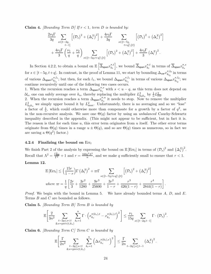
Claim 4. [Bounding Term D] If r < 1, term D is bounded by:

2ν2Γ

3q

∑

s∈[t−2q,t−1]

[(Ds

)2+(∆X

s

)2]+

4ν3Γ

3q

∑

s∈[t−7q,t+q]\{t}

[(Ds

)2+(∆X

s

)2]

+4ν4Γ

3

(ν1q

+ν2q

) ∑

s∈[t−5q,t+q]\{t}

[(Ds

)2+(∆X

s

)2]+

4ν4Γ

3

(∆X

t

)2.

In Section 4.2.2, to obtain a bound on E

[∆spanx

π,tkt

], we bound ∆spanx

π,tkt

in terms of ∆spanxπ,sks

for s ∈ [t−5q, t+q]. In contrast, in the proof of Lemma 11, we start by bounding ∆varxπ,l0kl0

in terms

of various ∆spanxπ,l1kl1

; but then, for each l1, we bound ∆spanxπ,l1kl1

in terms of various ∆spanxπ,l2kl2

; we

continue recursively until one of the following two cases occurs.1. When the recursion reaches a term ∆spanx

π,sks

with s < u − q, as this term does not depend on

Uu, one can safely average over ku, thereby replacing the multiplier L2k0ku

by 1nL

2res.

2. When the recursion reaches a term ∆spanxπ,uku

it needs to stop. Now to remove the multiplier

L2k0ku

we simply upper bound it by L2max. Unfortunately, there is no averaging and so we “lose”

a factor of 1n , which could otherwise more than compensate for a growth by a factor of q2, as

in the non-recursive analysis. We save one Θ(q) factor by using an unbalanced Cauchy-Schwartzinequality described in the appendix. (This might not appear to be sufficient, but in fact it is.The reason is that for each time u, this error term originates from u itself. The other error termsoriginate from Θ(q) times in a range u ± Θ(q), and so are Θ(q) times as numerous, so in fact weare saving a Θ(q2) factor.)

4.2.4 Finalizing the bound on Errt

We finish Part 2 of the analysis by expressing the bound on E [Errt] in terms of (Ds)2 and

(∆X

s

)2.

Recall that Λ2 =L2res

Γ2 + 1 and r = 160q2Λ2

n , and we make q sufficiently small to ensure that r < 1.

Lemma 12.

E [Errt] ≤( 15r

1− r

)Γ(∆X

t

)2+Γ

∑

s∈[t−7q,t+q]\{t}

[(Ds

)2+(∆X

s

)2]

where =1

q

[2r

3+

3r2

1280+

9r3

25600+

3r2

1− r+

r3

426(1 − r)+

r4

2844(1 − r)

].

Proof. We begin with the bound in Lemma 5. We have already bounded terms A, D, and E.Terms B and C are bounded as follows.

Claim 5. [Bounding Term B] Term B is bounded by

E

[2

3n2

∑

t−2q≤s<t&s=prev(t,ks)

n∑

kt=1

Γ ·(xπ(ks),tks

− xπ(kt),tks

)2]≤ ν1

15q

∑

s∈[t−2q,t−1]

Γ ·(Ds

)2.

Claim 6. [Bounding Term C] Term C is bounded by

E

[Γ

2n2

∑

t−2q≤s<t&s=prev(t,ks)

n∑

kt=1

(∆x

π(kt),sks

)2]≤ Γ

2n

∑

t−2q≤s≤t−1

(∆X

s

)2.

24

Summing up these bounds yields

E [Errt] ≤(2ν3n

+4ν43

+ ν4

)Γ(∆X

t

)2

+

[max

{ν115q

,3

2n

}+

2ν23q

+2(ν3 + ν4)

n+

7ν33q

+

(2ν3nq

+7ν43q

)(ν1 + ν2)

]

︸ ︷︷ ︸G

· Γ∑

s∈[t−7q,t+q]

((Ds)

2 +(∆X

s

)2). (13)

Via some elementary calculations, presented in Claim 7 in Appendix A.5, we show that thequantity G above can be bounded by

1

q

[2r

3+

3r2

1280+

9r3

25600+

3r2

1− r+

r3

426(1 − r)+

r4

2844(1 − r)

]

and that 2ν3n + 7ν4

3 ≤ 15r1−r as 1 ≤ q < n and r ≤ 1, which implies the bounds stated in the lemma.

4.3 Part 3: The Amortization

We let = 18 − 15r

1−r . From Lemmas 5 and 12, we obtain:

E[F (xt)− F (xt+1)

]≥ 1

3n2· E[ n∑

k=1

n∑

kt=1

Wk(gπ(kt,t),tk , x

π(kt,t),tk )

]

+ Γ(∆X

t

)2 −Γ∑

s∈[t−7q,t+q]

[(Ds

)2+(∆X

s

)2]. (14)

The term(∆X

s

)2and (Ds)

2 in (14) will be paid for by the progress terms from time s by means

of an amortization. Also, we will account for the term (Dt)2 using the bound from Lemma 10:

Γ · (Dt)2 ≤

(ν1q

+ν2q

)Γ

∑

s∈[t−5q,t+q]\{t}

((Ds

)2+(∆X

s

)2). (15)

For the purpose of amortizing the (Ds)2 terms, for some constant γ > 0 which we will specify

later, we add terms +γΓ (Dt)2 − γΓ (Dt)

2 to the bound from (14), and then we use (15) to bound(γ +)Γ (Dt)

2, which yields

E[F (xt)− F (xt+1)

]≥ 1

3n2· E[ n∑

k=1

n∑

kt=1

Wk(gπ(kt,t),tk , x

π(kt,t),tk )

]

+ (−) Γ(∆X

t

)2+ γΓ

(Dt

)2 −Γ∑

s∈[t−7q,t+q]\{t}

[(Ds

)2+(∆X

s

)2]

− ( + γ)

[(ν1q

+ν2q

)Γ

∑

s∈[t−5q,t+q]\{t}

((Ds

)2+(∆X

s

)2)]. (16)

25

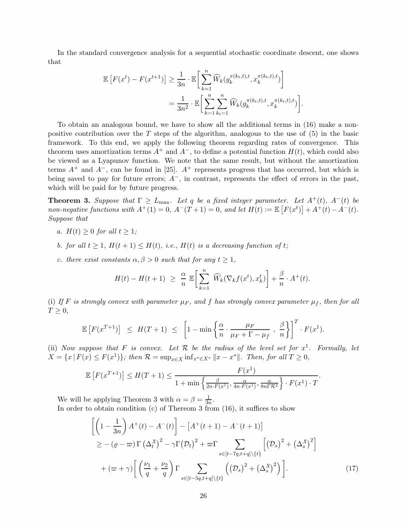
In the standard convergence analysis for a sequential stochastic coordinate descent, one showsthat

E[F (xt)− F (xt+1)

]≥ 1

3n· E[ n∑

k=1

Wk(gπ(kt,t),tk , x

π(kt,t),tk )

]

=1

3n2· E[ n∑

k=1

n∑

kt=1

Wk(gπ(kt,t),tk , x

π(kt,t),tk )

].

To obtain an analogous bound, we have to show all the additional terms in (16) make a non-positive contribution over the T steps of the algorithm, analogous to the use of (5) in the basicframework. To this end, we apply the following theorem regarding rates of convergence. Thistheorem uses amortization terms A+ and A−, to define a potential function H(t), which could alsobe viewed as a Lyapunov function. We note that the same result, but without the amortizationterms A+ and A−, can be found in [25]. A+ represents progress that has occurred, but which isbeing saved to pay for future errors; A−, in contrast, represents the effect of errors in the past,which will be paid for by future progress.

Theorem 3. Suppose that Γ ≥ Lmax. Let q be a fixed integer parameter. Let A+(t), A−(t) benon-negative functions with A+(1) = 0, A−(T +1) = 0, and let H(t) := E

[F (xt)

]+A+(t)−A−(t).

Suppose that

a. H(t) ≥ 0 for all t ≥ 1;

b. for all t ≥ 1, H(t+ 1) ≤ H(t), i.e., H(t) is a decreasing function of t;

c. there exist constants α, β > 0 such that for any t ≥ 1,

H(t)−H(t+ 1) ≥ α

nE

[ n∑

k=1

Wk(∇kf(xt), xtk)

]+

β

n·A+(t).

(i) If F is strongly convex with parameter µF , and f has strongly convex parameter µf , then for allT ≥ 0,

E[F (xT+1)

]≤ H(T + 1) ≤

[1−min

{α

n· µF

µF + Γ− µf,β

n

}]T· F (x1).

(ii) Now suppose that F is convex. Let R be the radius of the level set for x1. Formally, letX = {x |F (x) ≤ F (x1)}; then R = supx∈X infx∗∈X∗ ‖x− x∗‖. Then, for all T ≥ 0,

E[F (xT+1)

]≤ H(T + 1) ≤ F (x1)

1 + min{

β2n·F (x1)

, α4n·F (x1)

, α8nΓR2

}· F (x1) · T

.

We will be applying Theorem 3 with α = β = 13n .

In order to obtain condition (c) of Thereom 3 from (16), it suffices to show[(

1− 1

3n

)A+(t)−A−(t)

]−[A+(t+ 1)−A−(t+ 1)

]

≥ − (−) Γ(∆X

t

)2 − γΓ(Dt

)2+Γ

∑

s∈[t−7q,t+q]\{t}

[(Ds

)2+(∆X

s

)2]

+ ( + γ)

[(ν1q

+ν2q

)Γ

∑

s∈[t−5q,t+q]\{t}

((Ds

)2+(∆X

s

)2)]. (17)

26

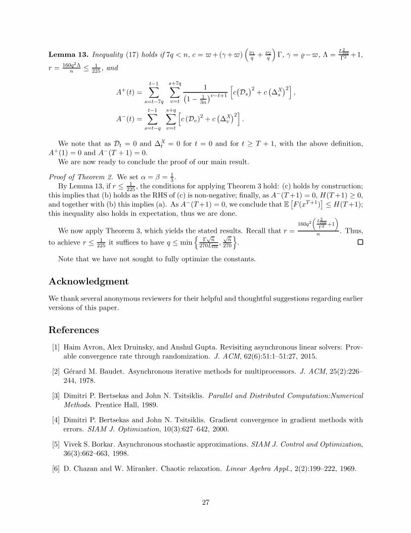
Lemma 13. Inequality (17) holds if 7q < n, c = +(γ+)(ν1q + ν2

q

)Γ, γ = −, Λ =

L2res

Γ2 +1,

r = 160q2Λn ≤ 1

225 , and

A+(t) =t−1∑

s=t−7q

s+7q∑

v=t

1(1− 1

3n

)v−t+1

[c(Ds

)2+ c

(∆X

s

)2],

A−(t) =t−1∑

s=t−q

s+q∑

v=t

[c (Dv)

2 + c(∆X

v

)2].

We note that as Dt = 0 and ∆Xt = 0 for t = 0 and for t ≥ T + 1, with the above definition,

A+(1) = 0 and A−(T + 1) = 0.We are now ready to conclude the proof of our main result.

Proof of Theorem 2. We set α = β = 13 .

By Lemma 13, if r ≤ 1225 , the conditions for applying Theorem 3 hold: (c) holds by construction;

this implies that (b) holds as the RHS of (c) is non-negative; finally, as A−(T+1) = 0, H(T+1) ≥ 0,and together with (b) this implies (a). As A−(T+1) = 0, we conclude that E

[F (xT+1)

]≤ H(T+1);

this inequality also holds in expectation, thus we are done.

We now apply Theorem 3, which yields the stated results. Recall that r =160q2

(

L2res

Γ2 +1

)

n . Thus,

to achieve r ≤ 1225 it suffices to have q ≤ min

{Γ√n

270Lres,√n

270

}.

Note that we have not sought to fully optimize the constants.

Acknowledgment

We thank several anonymous reviewers for their helpful and thoughtful suggestions regarding earlierversions of this paper.

References

[1] Haim Avron, Alex Druinsky, and Anshul Gupta. Revisiting asynchronous linear solvers: Prov-able convergence rate through randomization. J. ACM, 62(6):51:1–51:27, 2015.

[2] Gerard M. Baudet. Asynchronous iterative methods for multiprocessors. J. ACM, 25(2):226–244, 1978.

[3] Dimitri P. Bertsekas and John N. Tsitsiklis. Parallel and Distributed Computation:NumericalMethods. Prentice Hall, 1989.

[4] Dimitri P. Bertsekas and John N. Tsitsiklis. Gradient convergence in gradient methods witherrors. SIAM J. Optimization, 10(3):627–642, 2000.

[5] Vivek S. Borkar. Asynchronous stochastic approximations. SIAM J. Control and Optimization,36(3):662–663, 1998.

[6] D. Chazan and W. Miranker. Chaotic relaxation. Linear Agebra Appl., 2(2):199–222, 1969.

27

[7] Gong Chen and Marc Teboulle. Convergence analysis of a proximal-like minimization algorithmusing Bregman’s function. SIAM J. Optimization, 3(3):538–543, 1993.

[8] Yun Kuen Cheung and Richard Cole. Amortized analysis of asynchronous price dynamics. In26th Annual European Symposium on Algorithms, ESA 2018, August 20-22, 2018, Helsinki,Finland, pages 18:1–18:15, 2018.

[9] Yun Kuen Cheung, Richard Cole, and Nikhil R. Devanur. Tatonnement beyond gross substi-tutes? gradient descent to the rescue. In STOC, pages 191–200, 2013.

[10] Yun Kuen Cheung, Richard Cole, and Yixin Tao. Parallel Stochastic Asynchronous CoordinateDescent: Tight Bounds on the Possible Parallelism. arXiv e-prints, page arXiv:1811.05087,November 2018.

[11] Richard Cole and Yixin Tao. An Analysis of Asynchronous Stochastic Accelerated CoordinateDescent. arXiv e-prints, page arXiv:1808.05156, Aug 2018.

[12] Corinna Cortes and Vladimir Vapnik. Support-vector networks. Mach. Learn., 20(3):273–297,September 1995.

[13] Cong Fang, Yameng Huang, and Zhouchen Lin. Accelerating asynchronous algorithms forconvex optimization by momentum compensation. arXiv preprint arXiv:1802.09747, 2018.

[14] Andreas Frommer and Daniel B. Szyld. On asynchronous iterations. Journal of Computationaland Applied Mathematics, 123(1-2):201–216, 2000. Numerical Analysis 2000. Vol. III: LinearAlgebra.

[15] Robert Hannah, Fei Feng, and Wotao Yin. A2bcd: An asynchronous accelerated block coor-dinate descent algorithm with optimal complexity. 2018.

[16] Remi Leblond, Fabian Pedregosa, and Simon Lacoste-Julien. Improved asynchronous paralleloptimization analysis for stochastic incremental methods. J. Mach. Learn. Res., 19:81:1–81:68,2018.

[17] Ji Liu and Stephen J. Wright. Asynchronous stochastic coordinate descent: Parallelism andconvergence properties. SIAM Journal on Optimization, 25(1):351–376, 2015.

[18] Ji Liu, Stephen J. Wright, Christopher Re, Victor Bittorf, and Srikrishna Sridhar. An asyn-chronous parallel stochastic coordinate descent algorithm. Journal of Machine Learning Re-search, 16:285–322, 2015.

[19] Zhaosong Lu and Lin Xiao. On the complexity analysis of randomized block-coordinate descentmethods. Mathematical Programming, 152(1-2):615–642, 2015.

[20] H. Mania, X. Pan, D. Papailiopoulos, B. Recht, K. Ramchandran, and M. Jordan. Perturbediterate analysis for asynchronous stochastic optimization. SIAM Journal on Optimization,27(4):2202–2229, 2017.

[21] Lukas Meier, Sara Van De Geer, and Peter Bhlmann. The group lasso for logistic regression.Journal of the Royal Statistical Society: Series B (Statistical Methodology), 70(1):53–71, 2008.

[22] Yu. Nesterov. Introductory Lectures on Convex Optimization: A Basic Course. Springer US,2004.

28

[23] Yu. Nesterov. Efficiency of coordinate descent methods on huge-scale optimization problems.SIAM J. Optimization, 22(2):341–362, 2012.

[24] Feng Niu, Benjamin Recht, Christopher Re, and Stephen J. Wright. Hogwild: A lock-freeapproach to parallelizing stochastic gradient descent. In NIPS, pages 693–701, 2011.

[25] Peter Richtarik and Martin Takac. Iteration complexity of randomized block-coordinate de-scent methods for minimizing a composite function. Mathematical Programming, 144(1-2):1–38, 2014.

[26] Craig Saunders, Alexander Gammerman, and Volodya Vovk. Ridge regression learning algo-rithm in dual variables. In Proceedings of the Fifteenth International Conference on MachineLearning, ICML ’98, pages 515–521, San Francisco, CA, USA, 1998. Morgan Kaufmann Pub-lishers Inc.

[27] Tao Sun, Robert Hannah, and Wotao Yin. Asynchronous coordinate descent under morerealistic assumptions. In I. Guyon, U. V. Luxburg, S. Bengio, H. Wallach, R. Fergus, S. Vish-wanathan, and R. Garnett, editors, Advances in Neural Information Processing Systems 30,pages 6182–6190. Curran Associates, Inc., 2017.

[28] Robert Tibshirani. Regression shrinkage and selection via the lasso. Journal of the RoyalStatistical Society, Series B, 58:267–288, 1994.

[29] Paul Tseng and Sangwoon Yun. A coordinate gradient descent method for nonsmooth sepa-rable minimization. Math. Program., 117(1-2):387–423, 2009.

[30] John N. Tsitsiklis, Dimitri P. Bertsekas, and Michael Athans. Distributed asynchronous de-terministic and stochastic gradient optimization algorithms. IEEE Transactions on AutomaticControl, 31(9):803–812, 1986.

[31] Stephen J Wright. Coordinate descent algorithms. Mathematical Programming, 151(1):3–34,2015.

29

A Omitted Proofs and Subsidiary Lemmas

We begin with the proof of Lemma 1. Next, in Appendix A.1, we prove Lemmas 2 and 3, thebasic progress lemmas. In Appendix A.2, we prove Lemma 5, the progress lemma for the generalanalysis. Then, in Appendix A.3, we give several bounds on how much W can change when one ofits arguments is altered, leading to proofs of Lemmas 6–8. We follow this, in Appendix A.4, withthe proof of the recursive bound given in Lemma 21, which is used to show Lemma 2. We continue,in Appendix A.5, with the proofs of the claims from Section 4.2.4. Finally, in Appendix A.6, weprove Theorem 3 and Lemma 13.

Proof of Lemma 1. Let Ub be an update to coordinate xj with start and finish times sb and fb,resp. Let Ua be the update to coordinate xj with the earliest start time before sb that commitslater than Ub, if any. Let Uc be the update to coordinate xj with the latest start time after sb thatcommits earlier than Ub, if any. Let the start and finish times for Ua and Uc be (sb, fb), and (sc, fc),resp. Note that the start and commit times of an update differ by at most q + 1 as there are atmost q interfering updates for each update.

Suppose the SCC order for Ub is s. If Ua does not exist then s ≥ sb; it is convenient to set(sa, fa) = (sb, fb) in this case. Similarly, If Uc does not exist then s ≤ sb; it is convenient to set(sc, fc) = (sb, fb) in this case. Then it is always the case that sa ≤ s ≤ sc.

Case i. s < sb.Then sa ≤ s < sb < fb < fa ≤ sa + q + 1. It follows that sb ≤ sa + q − 1 and hence s ≥ sb − q + 1.Also fb ≤ sb + q + 1 ≤ sa + q − 1 ≤ s+ q − 1.

Case ii. s > sb.Then sb < s ≤ sc < fc < fb ≤ sb + q + 1. It follows that s ≤ sb + q − 1 and fb ≤ s+ q.

Case iii. s = sb.Then fb ≤ s+ q + 1.

Therefore, for any updates, their SCC order s and their commit time fb satisfy s < fb ≤ s+q+1.Now we determine the SCC range for updates that might interfere Ub. Note that they have committime in the range [sb + 1, fb − 1].

Case i. s < sb.The commit time for possibly interfering updates is in the range [sb +1, fb − 1] ⊆ [s, s+ q− 2] andhence their SCC rank is in the range [s− (q + 1), s + q − 3] = [s− q − 1, s+ q − 3].

Case ii. s > sb.The commit time for possibly interfering updates is in the range [sb + 1, fb − 1] ⊆ [s− q + 2, s+ q]and hence their SCC rank is in the range [s − q + 2− (q + 1), s + q − 1] = [s− 2q + 1, s + q − 1].

Case iii. s = sb.The commit time for possibly interfering updates is in the range [sb +1, fb − 1] ⊆ [s+ 1, s+ q] andhence their SCC rank is in the range [s+ 1− (q + 1), s + q − 1] = [s− q, s+ q − 1].

For all q ≥ 1, this range is contained in [s− 2q + 1, s + q − 1].

A.1 The Basic Progress Lemmas, Lemmas 2 and 3

We recall two known results.

Lemma 14 (Three-Point Property, [7, Lemma 3.2]). For any proper, convex and lower semi-continuous function Y : R→ R and for any d− ∈ R, letd+ := argmaxd∈R

{−Y (d) − Γ(d− d−)2

}. Then for any d′ ∈ R,

Y (d′) + Γ(d′ − d−)2 ≥ Y (d+) + Γ(d+ − d−)2 + Γ(d′ − d+)2.

30

Lemma 15 ([29, Lemma 4]). For any g1, g2, x ∈ R and Γ ∈ R+,∣∣∣d(g1, x)− d(g2, x)

∣∣∣ ≤ 1Γ · |g1 − g2| .

We can now lower bound Wj(g, x) in terms of dj(g, x).

Lemma 16. For any g, x ∈ R and Γ ∈ R+, Wj(g, x) ≥ Γ

2

(dj(g, x)

)2.

Proof. We apply Lemma 14 with d− = d′ = 0, with Γ replaced by 12Γ, and Y (d) = gd − Ψ(x) +

Ψ(x + d). Then Wj(d, g, x) = −Y (d) − Γd2/2, and hence d+, as defined in Lemma 14, equals

dj(g, x). These yield

Y (0) ≥ Y (dj(g, x)) + Γ ·(dj(g, x)

)2.

Since Y (0) = 0 and −Y (dj(g, x)) = Wj(g, x) +Γ2

(dj(g, x)

)2, we are done.

We are now ready to show Lemmas 2 and 3; they follow directly from Lemma 17 below. Wewill use the following well-known observation: for any 1 ≤ k ≤ n, x ∈ R

n and r ∈ R,

f(x+ r · ek) ≤ f(x) +∇kf(x) · r +Lk

2· r2, (18)

where ek is unit vector along coordinate k.

Lemma 17. Suppose there is an update to coordinate j at time t according to rule (1), and supposethat Γ ≥ Lmax. Let gj = ∇jf(x

t) and gj = ∇jf(x). Then

F (xt)− F (xt+1) ≥ Γ

4(dj(gj , x

tj))

2 − 1

Γ· (gj − gj)

2

and F (xt)− F (xt+1) ≥ Wj(gj , xtj)−

1

Γ· (gj − gj)

2.

Proof. To avoid clutter, we use the shorthand dj := dj(gj , xtj) and dj := dj(gj , x

tj). By update rule

(1), dj = ∆xtj.

F (xt+1) = f(xt+1) + Ψj(xt+1j ) +

∑

k 6=j

Ψk(xt+1k )

≤ f(xt) + gj dj +Γ

2(dj)

2 +Ψj(xtj + dj) +

∑

k 6=j

Ψk(xtk)

(By (18), (1), and the assumption Γ ≥ Lmax ≥ Lj)

= F (xt) + gj dj +Γ

2(dj)

2 −Ψj(xtj) + Ψj(x

tj + dj) + (gj − gj)dj

= F (xt)− Wj(gj , xtj) + (gj − gj)dj .

Hence, F (xt)− F (xt+1) ≥ Wj(gj , xtj)− (gj − gj)dj .

31

Then we can apply Lemma 16 to prove the first inequality in Lemma 17:

F (xt)− F (xt+1) ≥ Wj(gj , xtj)− (gj − gj)dj ≥

Γ

2(dj)

2 − |gj − gj | · |dj |

≥ Γ

2(dj)

2 − 1

2

[2

Γ· (gj − gj)

2 +Γ

2(dj)

2

](by the AM-GM ineq.)

=Γ

4(dj)

2 − 1

Γ· (gj − gj)

2.

We prove the second inequality in Lemma 17 as follows:

F (xt)− F (xt+1) ≥ Wj(gj , xtj)− (gj − gj)dj ≥Wj(dj , gj , x

tj)− (gj − gj)dj

= Wj(dj , gj , xtj) + (gj − gj)dj − (gj − gj)dj

= Wj(gj , xtj) + (gj − gj)(dj − dj) ≥ Wj(gj , x

tj)− |gj − gj | · |dj − dj |

≥ Wj(gj , xtj)−

1

Γ(gj − gj)

2. (By Lemma 15.)

A.2 The Expected Progress, Lemma 5

Proof of Lemma 5. Recall that we write π(k, t) to denote the path in which coordinate kt at timet is replaced by coordinate k, and to reduce clutter we abbreviate this as π(k). Recall also that welet prev(t, k) denote the time of the most recent update to coordinate k, if any, in the time range[t− 2q, t− 1]; otherwise, we set it to t. From (3),

E[F (xt)− F (xt+1)

]

≥ 1

2nEπ

[ n∑

kt=1

Wkt(gπ(kt),tkt

), xπ(kt),tkt

)

]+

Γ

8

(∆X

t

)2 − 1

ΓE

[(gπ,tkt− gπ,tkt

)2]

=1

2nEπ

[ n∑

k=1

Wk(gπ(k),tk , x

π(k),tk )

]+

Γ

8

(∆X

t

)2 − 1

ΓE

[(gπ,tkt− gπ,tkt

)2]

≥ 1

2nEπ

[ n∑

k=1

1

n

n∑

kt=1

(2

3Wk(g

π(kt),tk , x

π(k),tk )− 4

3Γ

(gπ(k),tk − g

π(kt),tk

)2)]

+Γ

8

(∆X

t

)2 − 1

ΓEπ

[(gπ,tkt− gπ,tkt

)2 ](by Lemma 6).

For the next bound, we will be applying Lemma 7 to shift the xπ(k),tk parameter in Wk to

xπ,tk = xπ(kt),tk . Note that applying this lemma introduces additional terms (the case l > 0) only

if xk is updated at some time s ∈ [t − 2q, t − 1]; this means that k = ks where t − 2q ≤ s < t,and to avoid double counting the effect of updates to the same coordinate, we can further limit sto s = prev(t, k), or equivalently that t − 2q ≤ s < t and s = prev(t, ks). This yields the claimedresult.

A.3 Bounding How Much W and d Vary as a Function of Their Arguments

The next five lemmas concern an arbitrary coordinate xj . To avoid notational clutter, we write

W , W , d, and Ψ in lieu of Wj Wj , d, and Ψj, resp. Also, by x1 and x2 we will mean two possiblevalues of xj , and by g1 and g2 two possible values of gj .

32

We first present the proofs of Lemma 6 and 8. To prove Lemma 7, we will need two additionallemmas, to be presented below.

Proof of Lemma 6.

W (g1, x) = maxd∈R

W (d, g1, x) ≥W (d(g2), g1, x)

= −g1 · d(g2)− Γ · d(g2)2/2 + Ψ(x)−Ψ(x+ d(g2))

= −g2 · d(g2)− Γ · d(g2)2/2 + Ψ(x)−Ψ(x+ d(g2))

+ (g2 − g1) ·[d(g1) + (d(g2)− d(g1))

]

≥ W (g2, x)− |g1 − g2| ·∣∣d(g1)

∣∣− |g1 − g2| ·∣∣d(g2)− d(g1)

∣∣

≥ W (g2, x)− |g1 − g2| ·∣∣d(g1)

∣∣− 1

Γ(g1 − g2)

2 (By Lemma 15)

≥ W (g2, x)−1

Γ(g1 − g2)

2 − Γ

4(d(g1))

2 − 1

Γ(g1 − g2)

2 (AM-GM ineq.)

≥ W (g2, x)−2

Γ(g1 − g2)

2 − 1

2W (g1, x). (By Lemma 16)

Next, we demonstrate Lemma 8; it is a simple corollary of Lemma 15 and the following lemma.

Lemma 18. For any g, x1, x2 ∈ R,∣∣d(g, x1)− d(g, x2)

∣∣ ≤ |x1 − x2| .

Proof. For i = 1, 2, let di := d(g, xi). By the definition of d, for i = 1, 2, there exists a subgradientΨ′(xi + di) such that

g + Γ · di +Ψ′(xi + di) = 0.

If d1 = d2, we are done. If d1 > d2, then Ψ′(x1 + d1) < Ψ′(x2 + d2). Since Ψ is convex,x1 + d1 ≤ x2 + d2 and hence 0 < d1 − d2 ≤ x2 − x1.

If d2 > d1, by the same argument as above we have 0 < d2 − d1 ≤ x1 − x2.

Lemma 8 is a simple corollary of Lemmas 15 and 18.

Proof of Lemma 8.

(d(g1, x1)− d(g2, x2)

)2=(d(g1, x1)− d(g1, x2) + d(g1, x2)− d(g2, x2)

)2

≤ 2(d(g1, x1)− d(g1, x2)

)2+ 2

(d(g1, x2)− d(g2, x2)

)2

≤ 2 (x1 − x2)2 +

2

Γ2(g1 − g2)

2 .

The next two lemmas will be needed to prove Lemma 7.

Lemma 19 (W Shifting on x parameter). Let W (g, x1) = W (d1, g, x1) and W (g, x2) = W (d2, g, x2).Then

W (g, x1) + Ψ(x2)−Ψ(x1) ≥ W (g, x2)− g(x2 − x1)− Γd2(x2 − x1)−Γ

2· (x2 − x1)

2.

33

Proof. We use Lemma 14 with d− = 0, d+ = d1, and Y (d) = gd−Ψ(x1)+Ψ(x1+ d). We note thatY (d′)+ Γ

2 · d′2 = −W (d′, g, x1). Also, we observe that −W (d′, g, x1) is strongly convex with strong

convexity parameter Γ. As W (d′, g, x1) is maximized at d1, we conclude that −W (d′, g, x1) ≥−W (d1, g, x1) +

Γ2 (d1 − d′)2 = −W (g, x1) +

Γ2 (d1 − d′)2. Thus

Y (d′) +Γ

2· (d′)2 ≥ − W (g, x1) +

Γ

2· (d′ − d1)

2.

The above inequality holds for any d′. In particular, we pick d′ = x2 − x1 + d2, yielding

W (g, x1) ≥ −g(x2 − x1 + d2) + Ψ(x1) − Ψ(x2 + d2)−Γ

2· (x2 − x1 + d2)

2

+Γ

2· (x2 − x1 + d2 − d1)

2.

By adding Ψ(x2)−Ψ(x1) to both sides, we obtain

W (g, x1) + Ψ(x2)−Ψ(x1)

≥ −g(x2 − x1 + d2) + Ψ(x2)−Ψ(x2 + d2)−Γ

2· (x2 − x1 + d2)

2

+Γ

2· (x2 − x1 + d2 − d1)

2

= W (g, x2)− g(x2 − x1)− Γd2(x2 − x1)−Γ

2· (x2 − x1)

2 +Γ

2· (x2 − x1 + d2 − d1)

2

≥ W (g, x2)− g(x2 − x1)− Γd2(x2 − x1)−Γ

2· (x2 − x1)

2.

Lemma 20 (Ψ Shifting). Let W (g1, x1) = W (d1, g1, x1) and W (g2, x2) = W (d2, g2, x2). Then

Ψ(x2 + d2)−Ψ(x1 + d1) ≤ g2(x1 − x2 + d1 − d2) +Γ

2· (x1 − x2 + d1)

2.

Proof. By the definition of d2, we have the following inequality, which directly implies the onestated in the lemma.

−g2d2 −Γ

2· (d2)2 −Ψ(x2 + d2) ≥ − g2(x1 − x2 + d1)−

Γ

2· (x1 − x2 + d1)

2 −Ψ(x1 + d1).

Proof. of Lemma 7. Suppose the latest update to coordinate k occurred at time t. Also supposethat

• the changes to xk from xt−2qk to x

π(k),tk are d11, d12, · · · , d1ℓ;

• the changes to xk from xt−2qk to xπ,tk are d21, d22, · · · , d2ℓ.

Furthermore, let

gak := ∇kf(xπ,t) and d := argmax

dW (d, gak , x

π,tk ).

In other words, xπ(k),tk = xt−2q

k +∑ℓ

r=1 d1r and xπ,tk = xt−2qk +

∑ℓr=1 d2r.

34

By Lemma 19,

W (gak , xπ(k),tk ) + Ψ(xπ,tk )−Ψ(x

π(k),tk ) ≥ W (gak , x

π,tk )− gak · (xπ,tk − x

π(k),tk )

− Γd · (xπ,tk − xπ(k),tk ) − Γ

2· (xπ,tk − x

π(k),tk )2.

On the other hand, let gbk be the gradient used to compute the update d2ℓ. By Lemma 20, on

setting x2 = xπ,tk − d2ℓ and x1 = xπ(k),tk − d1ℓ, and noting that d1 = d1ℓ and d2 = d2ℓ, we obtain

Ψ(xπ,tk )−Ψ(xπ(k),tk ) ≤ gbk(x

π(k),tk − xπ,tk ) +

Γ

2(x

π(k),tk − xπ,tk + d2ℓ)

2.

Combining the above two inequalities, and letting δ := xπ,tk − xπ(k),tk , yields

W (gak , xπ(k),tk ) ≥ W (gak , x

π,tk ) + (gbk − gak) · δ − Γd · δ − Γ

2· δ2 − Γ

2· (d2ℓ − δ)2

≥ W (gak , xπ,tk )− 1

2Γ(gbk − gak)

2 − Γ

2δ2 − Γ(d− δ)δ − Γδ2 − Γ

2δ2

− Γ

2(d2ℓ)

2 +Γ

2· 2d2ℓ · δ −

Γ

2δ2

= W (gak , xπ,tk )− 1

2Γ(gbk − gak)

2 − 3

2Γδ2 − Γ

2(d2ℓ)

2 − Γ(d− δ)δ + Γ(d2ℓ − δ)δ

≥ W (gak , xπ,tk )− 1

2Γ(gbk − gak)

2 − 3

2Γδ2 − Γ

2(d2ℓ)

2 − Γ|d− d2ℓ| · |δ|

≥ W (gak , xπ,tk )− 1

2Γ(gbk − gak)

2 − 2Γδ2 − Γ

2(d2ℓ)

2 − Γ

2(d− d2ℓ)

2.

By Lemma 8,Γ

2· (d− d2ℓ)

2 ≤ Γ · (d2ℓ)2 +1

Γ· (gak − gbk)

2.

Thus, W (gak , xπ(k),tk ) ≥ W (gak , x

π,tk )− 3

2Γ· (gbk − gak)

2 − 2Γδ2 − 3Γ

2· (d2ℓ)2. (19)

A.4 The Recursive Analysis yielding a proof of Lemma 11

Recall that the definition of ∆u,∅maxx

π,sks

(see Section 4.2.1) assumes the first u−4q updates are alreadyfixed.

To prove Lemma 11, we will make use of a recursive bound on( ∑

l0∈[u−q,t+q]\{u}Lkl0 ,ku

(∆t,∅

spanxπ,l0kl0

))2

,

a bound that expresses the effect of performing one level of recursion, along with additional compu-tation — suitable overestimates, and the calculation of some expectations. This bound is presentedin the next lemma. It is applied repeatedly in order to prove Lemma 11.

Both lemmas make use of two techniques. It will be helpful to explain them upfront.

Unbalanced Cauchy-Schwartz Inequality To bound an expression of the form(∑1≤j≤q′ zj

)2, rather than have the bound q′

∑1≤j≤q′ z

2j , we would like to multiply a few of the zj

35

by just a constant. We achieve this with two applications of the usual Cauchy-Schwartz Inequality,and we illustrate this for the case that “a few” means two of the zj .

( ∑

1≤j≤q′

zj

)2≤ 2(zk + zl)

2 + 2( ∑

1≤j≤q′

j 6=k,l

zj

)2≤ 4(z2k + z2l ) + 2(q′ − 2)

∑

1≤j≤q′

j 6=k,l

z2j

≤ 4(z2k + z2l ) + 2q′∑

1≤j≤q′

j 6=k,l

z2j (this is just a convenient over-estimate).

Recentering Suppose a ≤ b, c ≤ d. Then b2 ≤ [c+ (d− a)]2 ≤ 2c2 +2(d− a)2. we use this boundwhen b denotes a value (of the form ∆xk) which varies over the different paths across which wewant to average, while the values c and d − a are unvarying. This is a technique we already usedin Section 4.2.2.

Lemma 21 is a bound on a sum of ∆var terms. However, we will start by obtaining a recursivebound on an analogous sum of ∆span terms. To this end, we define

Vm , E

[ ∑

l0∈[u−q,t+q]\{u}

( ∑

l1,l2,··· ,lm∈[u−q,t+q],all ls distinct, all ls 6=u,l0;all ls≤ts−1+q, where

ts−1=min{t,l0,l1,··· ,ls−1};Sm⊆{ls|kls=kls−1

}.

( ∏

ls∈Rm\Sm

where Rm

={l1,l2,··· ,lm}.

L2kls ,kls−1

Γ2

)

· L2kl0 ,ku

(∆

tm,Rm\{lm}span xπ,lmklm

)2 )]. (20)

We note that the second summation is over all choices of ls, 1 ≤ s ≤ m, and of Sm which satisfythe stated conditions. This comment also applies to similar subsequent summations.

Note that V3q = 0 and V0 = E

[∑l0∈[u−q,t+q]\{u} L

2kl0 ,ku

(∆

min{t,l0},∅span xπ,l0kl0

)2 ].

Also, lm−1 ≤ min{lm−1, tm−2 + q} ≤ tm−1 + q. (21)

Lemma 21 below gives our recursive bound; it is then used to prove Lemmas 22 and 11. Finally,we prove Lemma 21 via Lemma 23, which is stated right before the proof of Lemma 21.

Lemma 21. For t− 2q ≤ u ≤ t,

Vm−1 ≤ 40qVm + E

[ ∑

s∈[t−7q,t+q]\{u}120qΓ2

(Λ2)m+1

(4q)m

nm+1

((∆spanx

π,sks

)2+(∆xπ,sks

)2)]

(22)

+ E

[24L2

max

(Λ2)m

(4q)m

nm

((∆spanx

π,uku

)2+(∆xπ,uku

)2)]. (23)

Lemma 21 readily yields a bound on V0. Recall that r = 160q2Λ2

n .

Lemma 22.

V0 ≤3r2Γ2

160(1 − r)q2

∑

s∈[t−7q,t+q]\{u}

[(Ds

)2+(∆X

s

)2]+

3rΓ2

5q(1 − r)·[(Du)

2 +(∆X

u

)2].

36

Proof. We will apply Lemma 21 recursively to V0. Note that as m increases by 1, each sum

is multiplied by Λ2·(4q)n , and the first term has a multiplier of 40q (which is why we chose r =

40q · Λ2(4q)n ). We obtain

V0 ≤ (1 + r + r2 + · · · ) · E[( ∑

s∈[t−7q,t+q]\{u}

480q2Γ2(Λ2)2

n2

((∆spanx

π,sks

)2+(∆xπ,sks

)2)

+96q(Λ2)L2

max

n

((∆spanx

π,uku

)2+(∆xπ,uku

)2))]

≤ 3r2Γ2

160(1 − r)q2

∑

s∈[t−7q,t+q]\{u}

[(Ds

)2+(∆X

s

)2]+

3rΓ2

5q(1 − r)

[(Du

)2+(∆X

u

)2],

as Lmax ≤ Γ, r < 1, and replacing 160q2Λ2/n by r.

Recall that Rm−1 = {l0, l1, · · · , lm−1} and tm−1 = min{t, l0, l1, · · · , lm−1}. In the proofs ofLemmas 11 and 21, we define ∆tm−1xπ,sks

as follows. If s /∈ Aπ,tm−1 , then ∆tm−1xπ,sksis the value

of ∆xπ,skswhen Us reads all its inputs and makes its update immediately after first tm−1 − 4q − 1

updates committed; otherwise, ∆tm−1xπ,sks= ∆

tm−1,Rm−1

max xπ,sks. We make the following observation.

Observation 1. For m ≥ 1,i. If s ∈ [tm−1 − 4q, tm−1 + q] \ {u}, then ∆tm−1xπ,sks

∈[∆

tm−1,Rm−1

min xπ,sks,∆

tm−1,Rm−1max xπ,sks

];

ii. If s ∈ [tm−1 − 4q, tm−1 + q] \ {u}, then ∆tm−1xπ,sksis independent of Uu and Uv for v ∈ Rm−1;

iii. If s ∈ [t− 4q, t+ q] \ {u}, then ∆txπ,sks∈[∆

tm−1,∅min xπ,sks

,∆tm−1,∅max xπ,sks

];

iv. If s ∈ [t− 4q, t+ q], then ∆txπ,sksis independent of Uu.

Proof. i. When s ∈ Aπ,tm−1 , ∆txπ,sks= ∆

tm−1,Rm−1max xπ,sks

m and so the result is immediate. We also

note, for use in (ii), that in this case ∆txπ,sksis independent of Rm−1.

While if s /∈ Aπ,tm−1 , we argue as follows. Note that every element in Rm−1 is at least tm−1.By Lemma 1, the updates in Rm−1 have commit time at least tm−1 + 1, while each of the firsttm−1 − 4q − 1 updates have commit time at most tm−1 − 4q − 1 + q + 1 = tm−1 − 3q. Thus, in thiscase too, the updates in Rm−1 are excluded from the computation of update Us.

Also, by the definition of ∆txπ,sks, Us reads all its inputs and makes its update immediately after

first tm−1 − 4q − 1 updates committed, all updates in Aπ,tm−1 have been fixed before Us starts itsreads. Consequently (i) holds in this case too.

ii. We have already shown the independence for v ∈ Rm−1 in the proof of (i).For update Uu, first recall that tm−1 − 2q ≤ u. If s ∈ Aπ,tm−1 , we want to show that

∆tm−1,Rm−1

max xπ,sksis independent of Uu. By the definition of Aπ,tm−1 , Us commits earlier than some

update Up where p < tm−1 − 4q. By Lemma 1, the commit time of Up is at most p + q + 1 ≤tm−1 − 3q ≤ u − q, hence Us must commit before time u − q, and hence it is independent of Uuwhose start time is at least u − q + 1 by Lemma 1. If s /∈ Aπ,t, ∆txπ,sks

depends only on the firsttm−1 − 4q − 1 < u− 2q updates, and these updates must be independent of Uu by Lemma 1.

iii. The argument is similar to (i).iv. The argument is similar to (ii).

37

Proof of Lemma 11. For brevity, we write V =

(∑l0∈[t−4q,t+q]\{u} Lkl0 ,ku

∆t,∅varx

π,l0kl0

)2

. Recall that

V =

( ∑

l0∈[t−4q,t+q]\{u}Lkl0 ,ku

∆t,∅varx

π,l0kl0

)2

=

( ∑

l0∈[t−4q,t+q]\{u}Lkl0 ,ku

max{∆t,∅

spanxπ,l0kl0

,∣∣∆t,∅

maxxπ,l0kl0

∣∣,∣∣∆t,∅

minxπ,l0kl0

∣∣})2

.

By Observation 1(iii), recentering and applying the Cauchy-Schwarz inequality,

V ≤ 10q∑

l0∈[t−4q,t+q]\{u}L2kl0 ,ku

[(∆t,∅

spanxπ,l0kl0

)2+(∆txπ,l0kl0

)2]

≤ 10q∑

l0∈[u−q,t+q]\{u}L2kl0 ,ku

(∆t,∅

spanxπ,l0kl0

)2+ 10q

∑

s∈[t−4q,u−q)

L2ks,ku

(∆t,∅

spanxπ,sks

)2

+ 10q∑

s∈[t−4q,t+q]\{u}L2ks,ku

(∆txπ,sks

)2.

Note that by Lemma 9(ii), ∆t,∅spanx

π,l0kl0≤ ∆

min{t,l0},∅span xπ,l0kl0

. For s < u− q, ∆t,∅spanx

π,sks

is independent

of update Uu, as ∆t,∅spanx

π,sks

is independent of updates Uv for v > s + q. Also, as already noted,

∆txπ,sksis independent of ku by Observation 1(iv). Thus, taking the expectation of the previous

bound as ku varies, yields

Eku[V] ≤ Eku

[10q

∑

l0∈[u−q,t+q]\{u}L2kl0 ,ku

(∆

min{t,l0},∅span xπ,l0kl0

)2 ]

+ Eku

[10q

∑

s∈[t−4q,u−q)

L2res

n

(∆t,∅

spanxπ,sks

)2 ]

+ Eku

[10q

∑

s∈[t−4q,t+q]\{u}

L2res

n

(∆txπ,sks

)2 ].

Note that for s ∈ [t−4q, t+ q]\{u}, ∆txπ,sks,∆xπ,sks

∈ [∆minxπ,sks

,∆maxxπ,sks

]. Thus, by recentering,

38

(∆txπ,sks

)2≤ 2

(∆xπ,sks

)2+ 2

(∆spanx

π,skl0

)2. Then we average over all paths π:

E[V] ≤ E

[10q

∑

l0∈[u−q,t+q]\{u}L2kl0 ,ku

(∆

min{t,l0},∅span xπ,l0kl0

)2 ]

+ E

[30q

∑

s∈[t−4q,t+q]\{u}

L2res

n

((∆spanx

π,sks

)2+(∆xπ,sks

)2)]

≤ 3r2Γ2

16(1 − r)q

∑

s∈[t−7q,t+q]\{u}

[(Ds

)2+(∆X

s

)2]+

6rΓ2

1− r

[(Du

)2+(∆X

u

)2]

+ 30q∑

s∈[t−4q,t+q]\{u}

L2res

n

[(Ds

)2+(∆X

s

)2](by Lemma 22)

≤ 3r2Γ2

16(1 − r)q

∑

s∈[t−7q,t+q]\{u}

[(Ds

)2+(∆X

s

)2]+

6rΓ2

1− r·[(Du

)2+(∆X

u

)2]

+3rΓ2

16q

∑

s∈[t−4q,t+q]\{u}

[(Ds

)2+(∆X

s

)2] (as r =

160Λ2q2

nand Λ =

L2res

Γ2+ 1.

)

In the next lemma we bound(∆

tm−1,Rm−1\{lm−1}span x

π,lm−1

klm−1

)2.

Lemma 23. Suppose l0, l1, · · · ∈ [u−q, t+q]\{u}, ts = min{t, l0, l1, · · · , ls}, Rm−1 = {l0, l1, · · · , lm−1}and ls ≤ ts + q for s < m. Then

39

(∆

tm−1,Rm−1\{lm−1}span x

π,lm−1

klm−1

)2

≤ 40q∑

lm∈[tm−1−4q,min{lm−1−1,u−q−1}]\({u}∪Rm−1)and klm=klm−1[ (

∆tm−1,Rm−1

span xπ,lmklm

)2

︸ ︷︷ ︸F

+(∆tm−1xπ,lmklm

)2

︸ ︷︷ ︸G

]

+ 40q∑

lm∈[min{lm−1−1,u−q−1}+1,lm−1−1]\({u}∪Rm−1)and klm=klm−1[ (

∆tm−1,Rm−1

span xπ,lmklm

)2︸ ︷︷ ︸

H

+(∆tm−1xπ,lmklm

)2︸ ︷︷ ︸

I

]

+ 8 · 1(klm−1=ku and u≤lm−1) ·

[ (∆

tm−1,Rm−1

span xπ,uku

)2+(∆tm−1,Rm−1

max xπ,uku

)2 ]

︸ ︷︷ ︸J

+40q

Γ2

( ∑

lm∈[tm−1−4q,min{tm−1+q,u−q−1}]\({lm−1,u}∪Rm−1)(L2klmklm−1

(∆

tm−1,Rm−1

span xπ,lmklm

)2

︸ ︷︷ ︸K

+L2klmklm−1

(∆tm−1xπ,lmklm

)2

︸ ︷︷ ︸L

))

+40q

Γ2

( ∑

lm∈[min{tm−1+q,u−q−1}+1,tm−1+q]\({lm−1,u}∪Rm−1)(L2klmklm−1

(∆

tm−1,Rm−1

span xπ,lmklm

)2

︸ ︷︷ ︸M

+L2klmklm−1

(∆tm−1xπ,lmklm

)2

︸ ︷︷ ︸N

))

+8

Γ2· 1(u≤tm−1+q) · L2

kuklm−1

[(∆

tm−1,Rm−1

span xπ,uku

)2+(∆tm−1,Rm−1

max xπ,uku

)2]

︸ ︷︷ ︸O

. (24)

Proof. Recall that tm−1 = min{t, l0, l1, · · · , lm−1}, and Rm−1 contains lm−1. Also recall that

∆tm−1,Rvar xπ,sks

= max{∆tm−1,R

max xπ,sks−∆

tm−1,Rmin xπ,sks

,∣∣∆tm−1,R

max xπ,sks

∣∣ ,∣∣∣∆tm−1,R

min xπ,sks

∣∣∣}.

First, let’s expand the term

(∆

tm−1,Rm−1\{lm−1}span x

π,lm−1

klm−1

)2

=(∆tm−1,Rm−1\{lm−1}

max xπ,lm−1

klm−1

−∆tm−1,Rm−1\{lm−1}min x

π,lm−1

klm−1

)2,

By Lemma 8, and recalling that the definition of ∆tm−1

var xπ,lmklmallows the choice of whether to read

the results of updates Us with s ∈ [tm−1 − 4q, tm−1 + q], we obtain

40

(∆

tm−1,Rm−1\{lm−1}span x

π,lm−1

klm−1

)2

≤ 2

( ∑

lm∈[tm−1−4q,lm−1−1]\Rm−1

and klm=klm−1

∆tm−1,Rm−1

var xπ,lmklm

)2

+2

Γ2

(gtm−1 ,Rm−1,π,lm−1

max,klm−1

− gtm−1,Rm−1,π,lm−1

min,klm−1

)2

≤ 2

( ∑

lm∈[tm−1−4q,lm−1−1]\Rm−1

and klm=klm−1

∆tm−1,Rm−1

var xπ,lmklm

)2

+2

Γ2

( ∑

lm∈[tm−1−4q,tm−1+q]\Rm−1

Lklmklm−1·∆tm−1,Rm−1

var xπ,lmklm

)2

. (25)

By applying the unbalanced Cauchy-Schwarz inequality, the first term on the RHS of (25) canbe bounded as follows (the 5q in the first inequality occurs because by (21), lm−1 ≤ tm−1 + q, andhence the range for lm is of size at most 5q):

2

( ∑

lm∈[tm−1−4q,lm−1−1]\Rm−1

and klm=klm−1

∆tm−1,Rm−1

var xπ,lmklm

)2

≤ 4 · (5q)∑

lm∈[tm−1−4q,lm−1−1]\({u}∪Rm−1)and klm=klm−1

(∆

tm−1,Rm−1

var xπ,lmklm

)2

+ 4 · 1(klm−1=ku and u≤lm−1−1) ·

(∆

tm−1,Rm−1

var xπ,uku

)2. (26)

Again, by using an unbalanced Cauchy-Schwarz inequality, the second term on the RHS of (25)can be bounded as follows:

2

Γ2

( ∑

lm∈[tm−1−4q,tm−1+q]\Rm−1

Lklmklm−1·∆tm−1,Rm−1

var xπ,lmklm

)2

≤ 4(5q)

Γ2

∑

lm∈[tm−1−4q,tm−1+q]

\({u}∪Rm−1)

L2klmklm−1

(∆

tm−1,Rm−1

var xπ,lmklm

)2

+4

Γ2· 1(u≤tm−1+q) · L2

kuklm−1

(∆

tm−1,Rm−1

var xπ,uku

)2. (27)

Observation 1(i) implies that for any s = lm ∈ [tm−1 − 4q, tm−1 + q] \ {u},(∆

tm−1,Rm−1

min xπ,sks

)2,

(∆

tm−1,Rm−1max xπ,sks

)2 ≤(∣∣∆tm−1,Rm−1

span xπ,sks

∣∣ +∣∣∆tm−1xπ,sks

∣∣)2

, and consequently by recentering,

(∆

tm−1,Rm−1

var xπ,sks

)2≤ 2(∆

tm−1,Rm−1

span xπ,sks

)2+ 2(∆tm−1xπ,sks

)2. (28)

41

Similarly, since ∆tm−1,Rm−1

max xπ,uku∈[∆

tm−1,Rm−1

min xπ,uku,∆

tm−1,Rm−1

max xπ,uku

],

(∆

tm−1,Rm−1

var xπ,uku

)2≤ 2(∆

tm−1,Rm−1

span xπ,uku

)2+ 2(∆tm−1,Rm−1

max xπ,uku

)2. (29)

In summary, (25) is bounded by (26) and (27); we split the range of the first term in each ofthese bounds, and bound the ∆var terms as in (28) and (29). This yields the result.

We can now prove Lemma 21.

Proof of Lemma 21. Next, we bound the LHS of the inequality in Lemma 21. To obtain our bound,we start with (24) and multiply both sides by

( ∏

ls∈Rm−1\Sm−1

where Rm−1

={l1,l2,··· ,lm−1}.

L2klskls−1

Γ2

)L2kl0ku

,

and sum over all choices of l0, l1, · · · , lm−1, and over all choices of a set Sm−1 defined shortly, wherethese parameters satisfy the following constraints.i. l0, l1, · · · , lm−1 ∈ [u− q, t+ q].ii. All the ls are distinct and ls 6= u for all s.iii. Let ts−1 = min{t, l0, l1, · · · , ls−1}; ls ≤ ts−1 + q for all s.iv. Sm−1 ⊆ {ls|kls = kls−1

}.v. Let Rm−1 = {l1, l2, . . . , lm}; for all s ≥ 1, ls ∈ Rm−1 \ Sm−1.

This multiplication of the LHS term of (23) yields

E

[ ∑

l0∈[u−q,t+q]\{u}

( ∑

l1,l2,··· ,lm−1∈[u−q,t+q],all ls distinct, all ls 6=u,l0;all ls≤ts−1+q, where

ts−1=min{t,l0,l1,··· ,ls−1}all Sm−1⊆{ls|kls=kls−1

}.

( ∏

ls∈Rm−1\Sm−1

where Rm−1

={l1,l2,··· ,lm−1}.

L2klskls−1

Γ2

)

L2kl0ku

(∆

tm−1,Rm−1\{lm−1}span x

π,lm−1

klm−1

)2)]

,

which is Vm−1.On the RHS, we start by looking at terms H and M to obtain the recursive term Vm on the RHS

of the Lemma 21. We use the inequality(∆

tm−1,Rm−1

span xπ,lmklm

)2 ≤(∆

tm,Rm−1

span xπ,lmklm

)2, which holds by

Lemma 9(ii). The multiplication applied to these two terms yields

42

≤ E

[40q

∑

l0∈[u−q,t+q]\{u}

( ∑

l1,l2,··· ,lm∈[u−q,t+q],all ls distinct, all ls 6=u,l0;

all ls≤ts−1+q,wherets−1=min{t,l0,l1,··· ,ls−1};all Sm−1⊆{ls|kls=kls−1

and s≤m−1};klm=klm−1

.

( ∏

ls∈Rm−1\Sm−1

where Rm−1

={l1,l2,··· ,lm−1}.

L2klskls−1

Γ2

)L2kl0ku

·(∆

tm,Rm−1

span xπ,lmklm

)2)]

+ E

[40q

∑

l0∈[u−q,t+q]\{u}

( ∑

l1,l2,··· ,lm∈[u−q,t+q],all ls distinct, all ls 6=u,l0;all ls≤ts−1+q, where

ts−1=min{t,l0,l1,··· ,ls−1};Sm−1⊆{ls|kls=kls−1

and s≤m−1}.

( ∏

ls∈Rm−1\Sm−1

where Rm−1

={l1,l2,··· ,lm−1}.

L2klskls−1

Γ2

)

· L2kl0ku

·L2klmklm−1

Γ2

(∆

tm,Rm−1

span xπ,lmklm

)2)]

These two terms correspond to including lm in Sm and not including it in the constraint for Vm;in other words, summed together these two terms equal Vm.

We now analyze the remaining non-recursive terms.

Recall that Λ2 =L2res

Γ2 + 1. Term J is bounded as follows, as we explain below:

E

[ ∑

l0∈[u−q,t+q]\{u}

( ∑

l1,l2,··· ,lm−1∈[u−q,t+q]all ls distinct, all ls 6=u,l0;all ls≤ts−1+q, where

ts−1=min{t,l0,l1,··· ,ls−1};all Sm−1⊆{ls|kls=kls−1

}.

( ∏

ls∈Rm−1\Sm−1

where Rm−1

={l1,l2,··· ,lm−1}.

L2klskls−1

Γ2

)L2kl0ku

· 8 · 1 klm−1=ku

and u≤lm−1

[(∆

tm−1,Rm−1

span xπ,uku

)2+(∆tm−1,Rm−1

max xπ,uku

)2])]

≤ E

[ ∑

l0,l1,··· ,lm−1

∈[u−q,t+q]\{u}u≤tm−1+q

8L2max

(Λ2)m−1

nm

[(∆

tm−1,Rm−1

span xπ,uku

)2+(∆tm−1,Rm−1

max xπ,uku

)2] ]

. (30)

Recall that by (21), lm−1 ≤ tm−1 + q, justifying the bound on the sum. We first bound L2kl0ku

by

L2max. Then we can average, in turn, over the random coordinate choices of kl0 , kl1 , . . ., klm−1

. As

we will explain below, depending on whether each ls−1 is in Sm−1 or not, the averaging ofL2kls

kls−1

Γ2

over kls−1will provide either an 1

n or an 1n ·

L2res

Γ2 factor. To elaborate, the factor (Λ2)m−1

nm on theRHS is due to a combination of the following observations:

i. As in Section 4.2.2, the m−1 factors of

(

L2res

Γ2+1

)

n = Λ2

n are due to the expectation over the bundle

of n paths obtained by varying kls−1, which does not affect the terms ∆

t,Rm−1

span xπ,uku, ∆

t,Rm−1max xπ,uku

, as

43

ls−1 ∈ Rm−1 and ls−1 6= u. In more detail, there is always a term due to the case kls−1/∈ Sm−1,

which, on averaging, yields a term 1n ·

L2res

Γ2 ; when kls = kls−1, there is also a term for the case that

kls−1∈ Sm−1, which, on averaging, yields a term of the form 1

n ; in combination, they yield a termΛ2

n . (if ls ∈ Sm−1, then kls = kls−1, and in this case taking the expectation yields an 1/n factor).

ii. The extra factor of n in the denominator is due to the expectation of 1klm−1=ku.

For the remaining terms, first note that, on the RHS of (24), for any s ∈ [tm−1−4q, tm−1+q]\{u},∆tm−1xπ,sks

is independent of any updates in Rm−1 or update Uu by Observation 1(ii). In addition,

for s < u− q, ∆tm−1,Rm−1

span xπ,sksalso doesn’t depend on any updates in Rm−1 or update Uu.

For term F , note that on the RHS, lm is being renamed s. Here we can start by averaging over

ku, as lm ≤ u− q, which yields a factor ofL2res

n ≤ Γ2Λ2

n . The remaining m− 1 factors of Λ2

n are asbefore. The final factor of 1

n is due to the condition klm = klm−1.

E

[ ∑

l0∈[u−q,t+q]\{u}

( ∑

l1,l2,··· ,lm−1∈[u−q,t+q]all ls distinct, all ls 6=u,l0;all ls≤ts−1+q, where

ts−1=min{t,l0,l1,··· ,ls−1};all Sm−1⊆{ls|kls=kls−1

}.

( ∏

ls∈Rm−1\Sm−1

where Rm−1

={l1,l2,··· ,lm−1};

L2klskls−1

Γ2

)L2kl0ku

· 40q ·∑

lm∈[tm−1−4q,u−q−1]\({u}∪Rm−1)klm=klm−1

(∆

tm−1,Rm−1

span xπ,lmklm

)2

≤ E

[ ∑

l0,l1,··· ,lm−1

∈[u−q,t+q]\{u}

40qΓ2 (Λ2)m

nm+1

∑

s∈[tm−1

−4q,u−q)

(∆

tm−1,Rm−1

span xπ,sks

)2 ]. (31)

For the next expression, we sum terms G and I. Again, we can start by averaging over ku,as ∆tm−1xπ,lmklm

is independent of Uu by Observation 1(ii), as lm ∈ [tm−1 − 4q, lm−1 − 1] ⊂ [tm−1 −4q, tm−1 + q] (as can be seen by applying (21)).

E

[ ∑

l0∈[u−q,t+q]\{u}

( ∑

l1,l2,··· ,lm−1∈[u−q,t+q]all ls distinct, all ls 6=u,l0;all ls≤ts−1+q, where

ts−1=min{t,l0,l1,··· ,ls−1};all Sm−1⊆{ls|kls=kls−1

}.

( ∏

ls∈Rm−1\Sm−1

where Rm−1

={l1,l2,··· ,lm−1};

L2klskls−1

Γ2

)L2kl0ku

· 40q ·∑

lm∈[tm−1−4q,lm−1−1]\({u}∪Rm−1)klm=klm−1

(∆tm−1xπ,lmklm

)2

≤ E

[ ∑

l0,l1,··· ,lm−1

∈[u−q,t+q]\{u}

40qΓ2 (Λ2)m

nm+1

∑

s∈[tm−1−4q,lm−1−1]\{u}

(∆tm−1xπ,sks

)2 ]. (32)

For term K, there is an additional term L2klm

klm−1to average over; we bound it by

L2res

n .

44

E

[ ∑

l0∈[u−q,t+q]\{u}

( ∑

l1,l2,··· ,lm−1∈[u−q,t+q]all ls distinct, all ls 6=u,l0;all ls≤ts−1+q, where

ts−1=min{t,l0,l1,··· ,ls−1};all Sm−1⊆{ls|kls=kls−1

}.

( ∏

ls∈Rm−1\Sm−1

where Rm−1

={l1,l2,··· ,lm−1};

L2klskls−1

Γ2

)L2kl0ku

· 40q∑

lm∈[tm−1−4q,u−q−1]\({u}∪Rm−1)

L2klmklm−1

Γ2

(∆

tm−1,Rm−1

span xπ,lmklm

)2

≤ E

[ ∑

l0,l1,··· ,lm−1

∈[u−q,t+q]\{u}

40qΓ2L2res(Λ

2)m

Γ2nm+1

∑

s∈[tm−1−4q,u−q−1]

(∆

tm−1,Rm−1

span xπ,sks

)2 ]. (33)

For the next expression, the sum of terms L and N , we obtain

E

[ ∑

l0∈[u−q,t+q]\{u}

( ∑

l1,l2,··· ,lm−1∈[u−q,t+q]all ls distinct, all ls 6=u,l0;all ls≤ts−1+q, where

ts−1=min{t,l0,l1,··· ,ls−1};all Sm−1⊆{ls|kls=kls−1

}.

( ∏

ls∈Rm−1\Sm−1

where Rm−1

={l1,l2,··· ,lm−1};

L2klskls−1

Γ2

)L2kl0ku

· 40q ·∑

lm∈[tm−1−4q,tm−1+q]\({u}∪Rm−1)

L2klmklm−1

Γ2

(∆tm−1xπ,lmklm

)2

≤ E

[ ∑

l0,l1,··· ,lm−1

∈[u−q,t+q]\{u}

40qΓ2L2res(Λ

2)m

Γ2nm+1

∑

s∈[tm−1−4q,tm−1+q]\{u}

(∆tm−1xπ,sks

)2 ]. (34)

Finally, for term O, the bound is

E

[ ∑

l0∈[u−q,t+q]\{u}

( ∑

l1,l2,··· ,lm−1∈[u−q,t+q]all ls distinct, all ls 6=u,l0;all ls≤ts−1+q, where

ts−1=min{t,l0,l1,··· ,ls−1};all Sm−1⊆{ls|kls=kls−1

}.

( ∏

ls∈Rm−1\Sm−1

where Rm−1

={l1,l2,··· ,lm−1};

L2klskls−1

Γ2

)L2kl0ku

· 8 ·L2kuklm−1

Γ21u≤tm−1+q

[(∆

tm−1,Rm−1

span xπ,uku

)2+(∆tm−1,Rm−1

max xπ,uku

)2])]

≤ E

[ ∑

l0,l1,··· ,lm−1

∈[u−q,t+q]\{u}

u≤tm−1+q

8L2max

L2res(Λ

2)m−1

Γ2nm

[(∆

tm−1,Rm−1

span xπ,uku

)2+(∆tm−1,Rm−1

max xπ,uku

)2] ]

. (35)

Therefore, the sum of the bounds on the non-recursive terms, reordered as 32, 34, 31, 33, 30,35, equals

45

E

[ ∑

l0,l1,··· ,lm−1

∈[u−q,t+q]\{u}

∑

s∈[tm−1−4q,lm−1−1]\{u}

40qΓ2 (Λ2)m

nm+1

(∆tm−1xπ,sks

)2 ](36)

+ E

[ ∑

l0,l1,··· ,lm−1

∈[u−q,t+q]\{u}

∑

s∈[tm−1−4q,tm−1+q]\{u}

40qΓ2L2res(Λ

2)m

Γ2nm+1

(∆tm−1xπ,sks

)2 ](37)

+ E

[ ∑

l0,l1,··· ,lm−1

∈[u−q,t+q]\{u}

∑

s∈[tm−1−4q,u−q)\{u}

40qΓ2 (Λ2)m

nm+1

(∆

tm−1,Rm−1

span xπ,sks

)2 ](38)

+ E

[ ∑

l0,l1,··· ,lm−1

∈[u−q,t+q]\{u}

∑

s∈[tm−1−4q,u−q)\{u}

40qΓ2L2res(Λ

2)m

Γ2nm+1

(∆

tm−1,Rm−1

span xπ,sks

)2 ](39)

+ E

[8

∑

l0,l1,··· ,lm−1

∈[u−q,t+q]\{u}u≤tm−1+q

L2max

(Λ2)m−1

nm

((∆

tm−1,Rm−1

span xπ,uku

)2+(∆tm−1,Rm−1

max xπ,uku

)2)]

(40)

+ E

[ ∑

l0,l1,··· ,lm−1

∈[u−q,t+q]\{u}u≤tm−1+q

8L2max

L2res(Λ

2)m−1

Γ2nm

·((

∆tm−1,Rm−1

span xπ,uku

)2+(∆tm−1,Rm−1

max xπ,uku

)2)]

. (41)

To obtain the final result, we combine these bounds. We start by bounding the sum of (36)and (37) as follows. Noting that ∆tm−1xπ,sks

,∆xπ,uku∈[∆minx

π,uku

,∆maxxπ,uku

]for s ≤ tm−1 + q, by

recentering,(∆tm−1xπ,sks

)2≤ 2

(∆spanx

π,sks

)2+ 2

(∆xπ,sks

)2, we obtain

E

[ ∑

l0,l1,··· ,lm−1

∈[u−q,t+q]\{u}

∑

s∈[tm−1−4q,lm−1−1]\{u}

40qΓ2 (Λ2)m

nm+1

(∆tm−1xπ,sks

)2 ]

+ E

[ ∑

l0,l1,··· ,lm−1

∈[u−q,t+q]\{u}

∑

s∈[tm−1−4q,tm−1+q]\{u}

40qΓ2L2res(Λ

2)m

Γ2nm+1

(∆tm−1xπ,sks

)2 ]

≤ E

[ ∑

s∈[t−7q,t+q]\{u}

80qΓ2 (Λ2)m+1(4q)m

nm+1

((∆spanx

π,sks

)2+(∆xπ,sks

)2)]. (42)

The additional Λ2 is from 1+L2res

Γ2 on the LHS of (42), and the (4q)m is due to the t+ q− (u− q) ≤(t+ q)− (t− 3q) = 4q choices of l0, l1, · · · , lm−1. We also relax the range [tm−1− 4q, tm−1+ q] \ {u}and the range [tm−1 − 4q, lm−1 − 1] \ {u} to [t− 7q, t+ q] \ {u} as lm−1 ≤ t+ q, tm−1 + q ≤ t+ q,and tm−1 − 4q ≥ u− 5q ≥ t− 7q.

46

Next, we sum (38) and (39). As tm−1 = min{t, l0, · · · , lm−1} ≥ s− q, we obtain

E

[ ∑

l0,l1,··· ,lm−1

∈[u−q,t+q]\{u}

∑

s∈[tm−1−4q,u−q)\{u}

40qΓ2 (Λ2)m

nm+1

(∆

tm−1,Rm−1

span xπ,sks

)2 ]

+ E

[ ∑

l0,l1,··· ,lm−1

∈[u−q,t+q]\{u}

∑

s∈[tm−1−4q,u−q)\{u}

40qΓ2L2res(Λ

2)m

Γ2nm+1

(∆

tm−1,Rm−1

span xπ,sks

)2 ]

≤ E

[ ∑

s∈[t−7q,t+q]\{u}40qΓ2 (Λ

2)m+1(4q)m

nm+1

(∆spanx

π,sks

)2]. (43)

Adding (42) and (43) yields the term (22) on the RHS of Lemma 21.

Finally, we sum (40) and (41). For u ≤ tm−1+q, as ∆tm−1,Rm−1max xπ,uku

, ∆xπ,uku∈[∆minx

π,uku

,∆maxxπ,uku

],

by recentering(∆

tm−1,Rm−1max xπ,uku

)2≤ 2

(∆spanx

π,uku

)2+2(∆xπ,uku

)2, and

(∆

tm−1,Rm−1

span xπ,uku

)2≤(∆spanx

π,uku

)2.

E

[8

∑

l0,l1,··· ,lm−1

∈[u−q,t+q]\{u}u≤tm−1+q

L2max

(Λ2)m−1

nm

((∆

tm−1,Rm−1

span xπ,uku

)2+(∆tm−1,Rm−1

max xπ,uku

)2)]

+ E

[ ∑

l0,l1,··· ,lm−1

∈[u−q,t+q]\{u}u≤tm−1+q

8L2max

L2res(Λ

2)m−1

Γ2nm

·((

∆tm−1,Rm−1

span xπ,uku

)2+(∆tm−1,Rm−1

max xπ,uku

)2)]

≤ E

[24L2

max

(Λ2)m(4q)m

nm

((∆spanx

π,uku

)2+(∆xπ,uku

)2)].

This yields the term (23) on the RHS of Lemma 21, which concludes the proof.

A.5 The Claims from Section 4.2.4

Recall that π(k) ≡ π(k, t). The following observation will be useful.

Observation 2. For u < t, ∆t,∅maxx

π(kt),uku

≥ ∆t,∅maxx

π(ku),uku

, ∆t,∅minx

π(kt),uku

≤ ∆t,∅minx

π(ku),uku

, and thus

∆t,∅spanx

π(ku),uku

≤ ∆t,∅spanx

π(kt),uku

.

Proof. This is immediate from the fact that replacing ku by kt on path π allows more choices ofinput in calculating the update to xku .

Proof of Claim 5. [Bounding Term B] We begin by noting that

xπ(ks),tks

= xπ,t−2qks

+∑

t−2q≤u<t&ku=ks

∆xπ(ks),uku

= xπ,t−2qks

+∑

t−2q≤u<t&ku=ks

∆xπ(ku),uku

, and

xπ(kt),tks

= xπ,t−2qks

+∑

t−2q≤u<t&ku=ks

∆xπ(kt),uku

.

47

Note that as t− 2q ≤ u, and as the updates Ur are fixed for r < t− 4q on the RHS of the following

expression, we have ∆xπ(ku),uku

∈[∆t,∅

minxπ(ku),uku

,∆t,∅maxx

π(ku),uku

]. Also, as u < t, and by Observation 2,

the range[∆t,∅

minxπ(ku),uku

,∆t,∅maxx

π(ku),uku

]⊆[∆t,∅

minxπ(kt),uku

,∆t,∅maxx

π(kt),uku

]. Further note that ∆x

π(kt),uku

lies in the same range,[∆t,∅

minxπ(kt),uku

,∆t,∅maxx

π(kt),uku

].

Therefore,

E

[2

3n2

∑

t−2q≤s<t&s=prev(t,ks)

n∑

kt=1

Γ ·(xπ(ks),tks

− xπ(kt),tks

)2 ]

≤ 2Γ

3n2· E[ ∑

t−2q≤s<t&s=prev(t,ks)

n∑

kt=1

[ ∑

t−2q≤u<t&ku=ks

(∆t,∅

spanxπ(kt),uku

)]2]

≤ 2Γ · 2q3n2

· E[ n∑

kt=1

∑

t−2q≤u<t

(∆t,∅

spanxπ(kt),uku

)2 ](by the Cauchy-Schwarz inequality)

≤ 4q

3n

∑

u∈[t−2q,t−1]

Γ · (Du)2 =

ν115q

∑

s∈[t−2q,t−1]

Γ · (Ds)2 (recall that ν1 =

20q2

n )

Proof of Claim 3. [Bounding Term A] We begin by observing:

E

[ ∑

t−2q≤s<t& s=prev(t,ks)

n∑

kt=1

1

2n2Γ·(gπ(kt),sks

− gπ(kt),tks

)2 ]

≤ E

[ ∑

t−2q≤s<t

n∑

kt=1

1

2n2Γ·(gπ(kt),sks

− gπ(kt),tks

)2 ]. (44)

Note that gπ(kt),sks

and gπ(kt),tks

are on the same path π(kt). The difference of these two values is

bounded by a sum of terms of the form Lkl0ks·∣∣∆x

π(kt),l0kl0

∣∣, where l0 needs to satisfy two conditions:

1. l0 ∈ [s − 2q,max{s + q, t − 1}]; 2. If l0 ≥ t, Ul0 commits before Us reads coordinate xkl0 . As

t− 2q ≤ s < t, if l0 satisfies these conditions,∣∣∆x

π(kt),l0kl0

∣∣ ≤ max{∣∣∆t,∅

minxπ(kt),l0kl0

∣∣,∣∣∆t,∅

maxxπ(kt),l0kl0

∣∣}≤

48

∆t,∅varx

π(kt),l0kl0

. Thus

E

[ ∑

t−2q≤s<t

n∑

kt=1

1

2n2Γ·(gπ(kt),sks

− gπ(kt),tks

)2 ]

≤ E

[ ∑

t−2q≤s<t

n∑

kt=1

1

n2Γ

(( ∑

l0∈[s−2q,max{s+q,t−1}]\{s}Lkl0ks

∆t,∅varx

π(kt),l0kl0

)2

+(Lksks∆x

π(kt),sks

)2)]

≤ E

[ ∑

t−2q≤s<t

1

nΓ

(( ∑

l0∈[t−4q,t+q]\{s}Lkl0ks

∆t,∅varx

π,l0kl0

)2+(Lksks∆xπ,sks

)2)]

(recall that π = π(kt).)

Then, using Lemma 11 for the first inequality, Γ ≥ Lmax for the second inequality, and Lemma 10to bound Γ

(Dt

)2for the third inequality, yields

E

[ ∑

t−2q≤s<t& s=prev(t,ks)

n∑

kt=1

1

2n2Γ·(gπ(kt),prev(t,ks)ks

− gπ(kt),tks

)2 ]

≤ ν3Γ

qn

∑

t−2q≤s<t

∑

r∈[t−7q,t+q]\{s}

[(Dr

)2+(∆X

r

)2]+

∑

t−2q≤s<t

ν4Γ

n

[(Ds

)2+(∆X

s

)2]

+∑

t−2q<s<t

L2max

nΓ2· Γ(∆X

s

)2(as Lksks ≤ Lmax)

≤ 2(ν3 + ν4)

n· Γ

∑

s∈[t−7q,t+q]\{t}

[(Ds

)2+(∆X

s

)2]+

2ν3n· Γ[(Dt

)2+(∆X

t

)2]

+Γ

n

∑

s∈[t−2q,t−1]

(∆X

s

)2

≤ 2(ν3 + ν4)

n· Γ

∑

s∈[t−7q,t+q]\{t}

[(Ds

)2+(∆X

s

)2]+

Γ

n

∑

s∈[t−2q,t−1]

(∆X

s

)2

+2ν3n· Γ(ν1q

+ν2q

) ∑

s∈[t−5q,t+q]\{t}

[(Ds

)2+(∆X

s

)2]+

2ν3n· Γ(∆X

t

)2.

Proof of Claim 6. [Bounding Term C]

E

[Γ

2n2

∑

t−2q≤s<t&s=prev(t,ks)

n∑

kt=1

(∆x

π(kt),sks

)2 ]≤ E

[Γ

2n

∑

t−2q≤s<t

(∆xπ,sks

)2]

≤ Γ

2n

∑

t−2q≤s≤t−1

(∆X

s

)2.

49

Proof of Claim 4. [Bounding Term D] We bound the term

E

[2

3Γn2

∑nk=1

∑nkt=1 ·

(gπ(k),tk − g

π(kt),tk

)2 ]. We will use the term g

π(k),t−2qk as an intermediary to

allow us to compare values on two different paths, as follows.

2

3

(gπ(k),tk − g

π(kt),tk

)2≤ 4

3

(gπ(k),tk − g

π(k),t−2qk

)2+

4

3

(gπ(k),t−2qk − g

π(kt),tk

)2

≤ 4

3

(gπ(k),tk − g

π(k),t−2qk

)2+

4

3

(gπ(kt),t−2qk − g

π(kt),tk

)2, (45)

as gπ(k),t−2qk = g

π(kt),t−2qk since the gradients at xπ,t−2q do not depend on update Ut.

For the first term on the RHS of (45), we apply Lemma 11 for the third inequality, and thenapply Lemma 10 to bound the (Dt)

2 term which was generated by Lemma 11, as follows.

E

[1

n

n∑

k=1

4

3

(gπ(k),tk − g

π(k),t−2qk

)2 ]≤ E

[1

n

n∑

k=1

4

3

( ∑

t−2q≤l0≤t−1

Lkl0k∆x

π(k),l0kl0

)2]

≤ E

[1

n

n∑

k=1

4

3

( ∑

t−2q≤l0≤t−1

Lkl0k∆varx

π(k),l0kl0

)2]

≤ 4ν3Γ2

3q

∑

s∈[t−7q,t+q]\{t}

[(Ds)

2 +(∆X

s

)2]+

4ν4Γ2

3

[(Dt

)2+(∆X

t

)2]

≤ 4ν3Γ2

3q

∑

s∈[t−7q,t+q]\{t}

[(Ds

)2+(∆X

s

)2]

+4ν4Γ

2

3·(ν1q

+ν2q

) ∑

s∈[t−5q,t+q]\{t}

[(Ds

)2+(∆X

s

)2]+

4ν4Γ2

3·(∆X

t

)2. (46)

For the second term on the RHS of (45), for t− 2q ≤ s ≤ t − 1, as ∆xπ(kt),sks

and ∆t,{t}maxx

π(kt),sks

are in the range[∆t,∅

minxπ(kt),sks

,∆t,∅maxx

π(kt),sks

], by recentering and by the Cauchy-Schwarz inequality,

4

3

(gπ(kt),t−2qk − g

π(kt),tk

)2=

4

3

( ∑

s∈[t−2q,t−1]

Lks,k∆xπ(kt),sks

)2

=16

3q

∑

s∈[t−2q,t−1]

L2ks,k

((∆t,∅

spanxπ(kt),sks

)2+(∆t,{t}

maxxπ(kt),sks

)2).

This yields

E

[1

n2

n∑

k=1

n∑

kt=1

4

3

(gπ(kt),t−2qk − g

π(kt),tk

)2 ]

≤ E

[1

n2

n∑

kt=1

n∑

k=1

16

3q

∑

s∈[t−2q,t−1]

L2ks,k

((∆t,∅

spanxπ(kt),sks

)2+(∆t,{t}

maxxπ(kt),sks

)2)]

≤ E

[1

n2

n∑

kt=1

16

3q

∑

s∈[t−2q,t−1]

L2res

((∆t,∅

spanxπ(kt),sks

)2+(∆t,{t}

maxxπ(kt),sks

)2)].

50

By Lemma 9,(∆t,∅

spanxπ(kt),sks

)2≤(∆spanx

π(kt),sks

)2and

(∆

t,{t}maxx

π(kt)ks

)2≤ 2

(∆spanx

π(kt),sks

)2+

2(∆x

π(kt),sks

)2. Thus,

E

[1

n2

n∑

k=1

n∑

kt=1

4

3

(gπ(kt),t−2qk − g

π(kt),tk

)2 ]≤ 16qL2

res

n

∑

s∈[t−2q,t−1]

((Ds

)2+(∆X

s

)2)

≤ 2ν2Γ2

3q

∑

s∈[t−2q,t−1]

((Ds

)2+(∆X

s

)2). (47)

Combining (45), (46) and (47) yields the result.

Claim 7. The term G in (13) is bounded by 1q

[2r3 + 3r2

1280 + 9r3

25600 + 3r2

1−r +r3

426(1−r) +r4

2844(1−r)

].

Proof. Recall that r = 160q2

n ·(L2res

Γ2 + 1)

(see the second paragraph of Section 4.2.3). As stated

before Lemma 10, ν1 = 20q2

n , ν2 =24q2L2

res

nΓ2 , and as stated before Lemma 11, ν3 = 316

(r2

1−r + r),

ν4 =6r1−r . Also, note that 1

n ≤qn as q ≥ 1, ν1 + ν2 ≤ 3r

20 , and ν2 +24q2

n = 3r20 .

max

{ν115q

,3

2n

}+

8ν211q

+2(ν3 + ν4)

n+

7ν33q

+

(2ν3nq

+7ν43q

)(ν1 + ν2)

≤ 1

q

[max

{ν115

,3q2

2n

}+

8ν211

+

(3

4

(r2

1− r+ r

)+

24r

1− r

)r

320+

7

16

(r2

1− r+ r

)

+

(3

4

(r2

1− r+ r

)r

320+

14r

1− r

)3r

20

]

≤ 1

q

[r

(1

9+

7

16

)+ r2

3

1280+ r3

9

25600+

r2

1− r

(3

40+

7

16+

21

10

)

+r3

1− r

(3

1280

)+

r4

1− r

(9

25600

)]

≤ 1

q

[2r

3+

3r2

1280+

9r3

25600+

3r2

1− r+

r3

426(1 − r)+

r4

2844(1 − r)

].

A.6 Proofs for the Amortized Analysis, Section 4.3: Theorem 3 and Lemma 13

The following lemma is key to the demonstration of progress in both the strongly convex and convexcases.

For any t ≥ 1, we define: PRG(t) ,

n∑

k=1

Wk(∇kf(xt), xtk).

We will use the following lemma from [25, Lemmas 4,6]. The version we present here is slightlydifferent from the one in [25], but the proofs are essentially the same.

Lemma 24 ([25, Lemmas 4,6]).(a) Suppose that f, F are strongly convex with parameters µf , µF > 0 respectively, and suppose thatΓ ≥ µf . Then

PRG(t) ≥ µF

µF + Γ− µf· F (xt).

51

(b) Suppose that f, F are convex functions. Suppose that R := minx∗∈X∗ ‖xt − x∗‖ <∞. Then

PRG(t) ≥ min{12,F (xt)

2ΓR2

}· F (xt).

Proof of Theorem 3. We begin by showing (i). By assumption (c) and Lemma 24(a),

H(t)−H(t+ 1) ≥[αn· E[PRG(t)

]+

β

n·A+(t)

]

≥[αn· µF

µF + Γ− µf· E[F (xt)

]+

β

n· A+(t)

]≥ δ ·H(t),

where δ , min{αn ·

µF

µF+Γ−µf, βn}.

Thus H(t + 1) ≤ (1− δ)H(t) for all t ≥ 1. Iterating the above inequality T times yieldsH(T + 1) ≤ (1− δ)T H(1).

To finish the proof note that since A+(1) = 0 and A−(1) ≥ 0, H(1) ≤ F (x1).

Now we show (ii). By the second assumption, Lemma 24 and the fact that E[X2] ≥ E[X]2,

H(t)−H(t+ 1)

≥[αn· E[PRG(t)

]+

β

n· A+(t)

]≥[αn·min

{1

2,E[F (xt)]

2ΓR2

}· E[F (xt)] +

β

n· A+(t)

].

We consider two cases:

• If E[F (xt)] ≤ A+(t), then A+(t) ≥ H(t)2 , thus

α

n·min

{1

2,E[F (xt)]

2ΓR2

}· E[F (xt)] +

β

n·A+(t) ≥ β

2n·H(t).

• If E[F (xt)] > A+(t), then E[F (xt)] > H(t)2 , thus

α

n·min

{1

2,E[F (xt)]

2ΓR2

}· E[F (xt)] +

β

n·A+(t) >

α

2n·min

{1

2,H(t)

4Γ R2

}·H(t).

Since H is a decreasing function, H(t) ≤ H(1) ≤ F (x1). Thus, unconditionally,

α

n·min

{1

2,E[F (xt)]

2ΓR2

}· E[F (xt)] +

β

n·A+(t) ≥ min

{β

2n,α

4n,α ·H(t)

8nΓR2

}·H(t)

≥ min

{β

2n · F (x1),

α

4n · F (x1),

α

8nΓR2

}·H(t)2.

Note that the term min{

β2n F (x1)

, α4nF (x1)

, α8nΓR2

}is independent of t. We denote it by ε. Thus,

H(t)−H(t+ 1) ≥ ε H(t)2. Dividing both sides by H(t) ·H(t+ 1) yields

1

H(t+ 1)− 1

H(t)≥ ε

H(t)

H(t+ 1)≥ ε.

Iterating the above inequality T times yields1

H(T + 1)− 1

H(1)≥ εT,

and hence1

H(T + 1)≥ εT +

1

H(1)≥ εT +

1

F (x1). (since H(1) ≤ F (x1))

(ii) follows by taking the reciprocal on both sides of the above inequality.

52

Proof of Lemma 13. By calculation,

A+(t)−A+(t+ 1) =

t−1∑

s=t−7q

1(1− 1

3n

)[c(Ds

)2+ c(∆X

s

)2]

+

t−1∑

s=t−7q+1

s+7q∑

v=t+1

1

3n

1(1− 1

3n

)v−t+1

[c(Ds

)2+ c(∆X

s

)2]

−t+7q∑

v=t+1

1(1− 1

3n

)v−t

[c(Dt

)2+ c(∆X

t

)2]

=1

3nA+(t) +

t−1∑

s=t−7q

[c(Ds

)2+ c(∆X

s

)2]

−t+7q∑

v=t+1

1(1− 1

3n

)v−t

[c(Dt

)2+ c(∆X

t

)2]

A−(t+ 1)−A−(t) =t+q∑

v=t+1

[c (Dv)

2 + c(∆X

v

)2]−t−1∑

s=t−q

[c (Dt)

2 + c(∆X

t

)2].

Therefore[(

1− 1

3n

)A+(t)−A−(t)

]−[A+(t+ 1)−A−(t+ 1)

]

=

t−1∑

s=t−7q

[c(Ds

)2+ c(∆X

s

)2]−t+7q∑

v=t+1

1(1− 1

3n

)v−t

[c(Dt

)2+ c(∆X

t

)2]

+

t+q∑

v=t+1

[c(Dv

)2+ c(∆X

v

)2]−t−1∑

s=t−q

[c(Dt

)2+ c(∆X

t

)2]

=∑

s∈[t−7q,t+q]\{t}

[c(Ds

)2+ c(∆X

s

)2]

−( t+7q∑

v=t+1

1(1− 1

3n

)v−t + q

)[c(Dt

)2+ c(∆X

t

)2]. (48)

In order to achieve (17), we compare the coefficients of each of the terms c (Dt)2, c

(∆X

t

)2, c (Ds)

2,

c(∆X

s

)2in (17) and (48). Since c = + (γ +)

(ν1q + ν2

q

)Γ the coefficient of (Ds)

2 and(∆X

s

)2in

(48) is at least as big as in (17). Therefore, it suffices to have the coefficients of (Dt)2 and

(∆X

t

)2satisfy the following inequalities.

γ ≥ c

Γ·[ 7q∑

i=1

1(1− 1

3n

)i + q

]

=1

q[q + (γ +) (ν1 + ν2)] ·

[3n

(1

(1− 1

3n

)7q+1 −1

1− 13n

)+ q

]

53

and − ≥ 1

q[q + (γ +)(ν1 + ν2)] ·

[3n

(1

(1− 1

3n

)7q+1 −1

1− 13n

)+ q

].

If 7q < 3n − 2, then by the fact that (1 + x)s ≤ 1 + sx1−(s−1)x for any x < 1

s−1 and s ≥ 1,

3n

(1

(1− 1

3n

)7q+1 −1

1− 13n

)+ q ≤ 3n

[(1 +

1

3n− 1

)7q+1− 3n

3n− 1

]+ q

≤ 3n

[1 +

(7q + 1)(

13n−1

)

1− 7q3n−1

− 1

]+ q

≤ 3n

(7q + 1

3n− 1− 7q

)+ q ≤ 14q + 2 + q,

if 3n3n−1−7q ≤ 2, i.e., if 7q ≤ n− 1.

Then it suffices that γ ≥ 1

q[q + (γ +)(ν1 + ν2)] (15q + 2)

and − ≥ 1

q[q + (γ +)(ν1 + ν2)] (15q + 2).

Recall that ν1 = 20q2

n ≤ r8 and ν2 =

24q2L2res

nΓ2 ≤ r6 , = 1

8 − 15r1−r (see the first line of Section 4.3),

and = 1q

[2r3 + 3r2

1280 + 9r3

25600 + 3r2

1−r +r3

426(1−r) +r4

2844(1−r)

]. One choice of values that suffices is

γ = − and r ≤ 1225 .

54

A Table of Definitions and Parameters

Notation / Definition / Description First

Parameter Appearance

F : Rn → R F (x) = f(x) +∑n

k=1Ψk(xk)

f : Rn → R F is the convex function we Abstract

Ψk : R→ R want to minimize.

ej the unit vector along coordinate j

Definition 1

Ljk |∇kf(x+ r · ej)−∇kf(x)| ≤ Ljk · |r|Lres ||∇f(x+ r · ej)−∇f(x)|| ≤ Lres · |r|

Lres Lres , maxk

(∑nj=1(Lkj)

2)1/2

LmaxLmax , maxj,k Ljk

if f is twice differentiable, then Lmax = maxj Ljj

µf , µF

strong convexity parameters of f, F

f(y)− f(x) ≥ 〈∇f(x), y − x〉+ 12µf ||y − x||2 Definition 2

F (y)− F (x) ≥ 〈∇F (x), y − x〉+ 12µF ||y − x||2

Ut the t-th update (in the SCC order)

Γ parameter used in the update rule

Wj(d, g, x) Wj(d, g, x) , gd+ Γd2/2 + Ψj(x+ d)−Ψj(x)

Wj(g, x) Wj(g, x) , maxd W (d, g, x) Near

dj(g, x) dj(g, x) , argmaxdW (d, g, x) Eqn. (1)

asynchronous xt+1j ← xtj + dj(gj , x

tj),

update rule where gj is the (inaccurate) measured gradient.

q

the updates that can interfere with the update

at time t in the ST order are those that Assumption 4

commit at times t+ 1, t+ 2, · · · , t+ q

∆xπ,tktthe increment computed by the t-th update on path π Near Lemma 1

kt the coordinate that is updated at time t Beginning

gtkgtk , ∇kf(x

t) of

accurate gradient along coordinate k at time t Section 3

π a root-to-leaf path in the branching tree

π(k, t)the root-to-leaf path with time t Beginning of

coordinate on path π replaced by coordinate k Section 3.2

π(kt, t) π(kt, t) = π

•π,t for any variable •, •π,t denotes its valueat time t along the path π

55

Notation / Definition / Description First

Parameter Appearance

Aπ,uAπ,u = {r|u− 4q ≤ r < u− 2q and Ur has committed

Section 4.2.1

before some Up for p ≤ u− 4q − 1}

∆u,R,Smax xπ,sks

see the table in the next page

∆u,Rmaxx

π,sks

∆u,Rmaxx

π,sks

, maxS ∆u,R,Smax xπ,sks

∆u,Rspanx

π,sks

∆u,Rspanx

π,sks

, ∆u,Rmaxx

π,sks−∆u,R

minxπ,sks

∆umaxx

π,sks

∆umaxx

π,sks

, ∆u,∅maxx

π,sks

∆u,Rvar x

π,sks

∆u,Rvar x

π,sks

, max{∆u,R

spanxπ,sks

,∣∣∆u,R

maxxπ,sks

∣∣,∣∣∆u,R

minxπ,sks

∣∣}

Section 4.2.1

∆Rmaxx

π,sks

∆Rmaxx

π,sks

, maxs−q≤t≤s∆t,Rmaxx

π,sks

∆Rspanx

π,sks

∆Rspanx

π,sks

, ∆Rmaxx

π,sks−∆

Rminx

π,sks

∆Rvarx

π,sks

∆Rvarx

π,sks

, max{∆

Rspanx

π,sks

,∣∣∆R

maxxπ,sks

∣∣,∣∣∆R

minxπ,sks

∣∣}

∆maxxπ,sks

∆maxxπ,sks

, ∆∅maxx

π,sks

∆spanxπ,sks

∆spanxπ,sks

, ∆∅spanx

π,sks

∆varxπ,sks

∆varxπ,sks

, ∆∅varx

π,sks

gu,R,S,π,smax,ks

see the next table

gu,R,π,smax,ks

gu,R,π,smax,ks

= maxS⊆[u−4q,u+q]\(Aπ,u∪{s}) gu,R,S,π,smax,ks

gR,π,smax,ks

gR,π,smax,ks

= maxs−q≤u≤s gu,R,π,smax,ks

gπ,smax,ksgπ,smax,ks

= g∅,π,smax,ks

gπ,sspan,ksgπ,sspan,ks

, gπ,smax,ks− gπ,smin,ks

(Dt)2 (Dt)

2, E

[(∆maxx

π,tkt−∆minx

π,tkt

)2]Section 4.2.1

(∆X

t

)2 (∆X

t

)2, E

[(∆xπ,tkt

)2]

The time of the most recent update to

prev(t, k) coordinate k, if any, in the time range Lemma 7

[t− 2q, t− 1]; otherwise, we set it to t.

ν1, ν2 ν1 ,20q2

n and ν2 ,24q2L2

res

nΓ2 Lemma 10

56

Notation / Definition / Description First

Parameter Appearance

Λ, r Λ ,L2res

Γ2 + 1 and r ,160q2

n · Λ2

Lemma 11ν3, ν4 ν3 ,

316

(r2r1−r + r

)and ν4 ,

6r1−r

Vm Eqn. (20)

∆tm−1xπ,sksBefore Observation 1

, 1q

[2r3 + 3r2

1280 + 9r3

25600 + 3r2

1−r +r3

426(1−r) +r4

2844(1−r)

]Lemma 12

, 18 − 15r

1−r Section 4.3

γ a parameter introduced for amortization Eqn. (16)

c c , + (γ +)(ν1q + ν2

q

)Lemma 13

For any set R,S ⊂ [u− 4q, u+ q] \Aπ,u ∪ {s}, when the first (u− 4q − 1) updates on

path π have been fixed, and update Uv is excluded from the computation of Us for

v ∈ R ∪ S and for v > u+ q; for all r ∈ Aπ,u, the value of the update Ur is already fixed,

then:

∆u,R,Smax xπ,sks

, the maximum value that ∆xπ,skscan assume

gu,R,S,π,smax,ks

, the maximum value of gπ,skscan assume

57