International Hydrographic Review, Monaco, LX X(l), M arch 1993

OPTIMAL LINE SPACING IN HYDROGRAPHIC SURVEY

by E.C. BOUWMEESTER and A.W. HEEMINK 1

INTRODUCTION

In this paper the authors present a simple, straightforward method, that provides a quantitative criterion for the optimal line spacing of a hydrographic survey. Their aim is to estimate the depth between the sounding lines and to also obtain the interpolation error variance of the depth estimate To achieve this goal they assume the seabottom to be a realisation of a stationary Gaussian random field with known mean and covariance function. Using least squares techniques, the derivation of the linear minimum variance estimator for the depth between sounding lines becomes straightforward. In order to obtain estimates of the mean and covariance function of the seabottom, measurements have to be taken along a few lines perpendicular to the usual direction of the sounding lines. Finally, a relation between the interpolation error variance and line spacing is obtained.

HYDROGRAPHIC SURVEY

The purpose of any hydrographic survey is to obtain a predefined accurate insight of the characteristics of the seabottom. The following marine activities heavily depend on information about the seabed :

1) Nautical charting: the production of charts for navigational purposes;

2) Maintenance and control of harbour approaches of deep draft shipping routes;

3) Optimisation of dredging operations;4) Scientific marine research.

All these activities have their own demands with regard to the quality of the hydrographic survey. However, it is well known that the differences in the

1 Tidal Waters Division, Rijkswaterstaat, Postbus 20907, 2500 EX, the Hague, the Netherlands.

required quality of the hydrographic surveys for these different activities all depend on the selected line spacing.

The need for a quantitative approach to estimate the quality of a sounding operation is self evident. The specific goal of any hydrographic survey, using sonic depth measurement and running parallel sounding lines over the area, has to be formulated in terms of a desired accuracy criterion. Only then, is it possible to optimize line spacing density. Although no two surveys are alike, the authors believe that the different goals of each hydrographic survey finally result in only a different accuracy standard. Since the accuracy of a hydrographic survey is, to large extent, governed by the line spacing, it is desirable to obtain a relation between line spacing density and survey accuracy.

Depending on the specific goal of the survey, accuracy standards have to be defined. Then a sounding plan can be drawn up that meets the accuracy requirements. The usual method of sonic depth measurement consists of running a succession of parallel sounding lines across the survey area. The resulting sounding procedure cannot provide complete coverage of the seabottom. The coverage of the seabottom obtained depends on the water depth, the line spacing and the echo sounder's beam width. For a typical Dutch situation, encountered in harbour approach channels, with depths of about 25 meters, the line spacing is typically about 50 meters. Using an Atlas Deso 20 echo sounder, with a beam width of 7 degrees, only 6% coverage of the actual seabottom is obtained. Since the main concern of this type of hydrographic survey is to find all obstructions which may endanger navigation, there is a need for a quantitative criterion of the quality of the survey. Of particular interest, is the relation between the sounding procedure and the probability of missing a high spot.

The usual approach to obtain optimal survey quality is of a heuristic nature. It is argued that by running the sounding lines perpendicular to the direction of the depth contours, the probability of missing a high spot will be minimal. If it is believed that the desired accuracy cannot be achieved in this way, the conventional sounding operation may be modified by running intermediate lines (interlines) to increase the density of area coverage, or cross­lines to obtain an improved angle of cut of the contours. The drawback of this heuristic method is that a priori characteristics of the seabed must be available to find the best direction in which the sounding lines have to be run. Secondly, this method assumes a pronounced anisotropy in the one direction on which a pre­selected direction of sounding lines is based. Another problem of this heuristic approach is the inherent difficulty of finding an optimal line spacing. The hydrographic survey procedure relies on the belief that an improvement of sounding accuracy can be achieved by increasing sounding line density, without quantitatively checking this belief. So, it is possible using the heuristic method to achieve satisfactory (= improving accuracy) coverage of the seabed with minimum costs.

CLOET (CLOET, 1976) has carried out a heuristic approach for a strip of survey area about 400 meters wide and 4 km long, lying along the main inward route into the North Sea, close to the survey area described in this paper. This strip has been surveyed with a 'saturation line spacing'. In order to get a measure of survey errors due to line spacing, CLOET selected line spadngs of 30, 60 and

100 meters. The survey error is then defined as follows. The depths from the selected line sparings are compared with the depths found in the intervening saturation lines. The error is called positive if the value on the saturation track is shallower than the depth on the selected line. Then, C lo e t evaluated the statistics of the survey errors and derived a relation between line spacing and the standard deviation of the survey error a in meters:

0 = 0.15 + 3.0 x lO^L

with L the line spacing in meters. In the discussion this formula will be examined in relation to data obtained by the authors.

FIELD DATA

A survey was carried out to provide the necessary extra sounding lines, perpendicular to those lines routinely measured. The survey was carried out on 10 March 1988 in the North Hinder area, covering a sandwave field of approximately 4 km by 3 km (fig. 1). This area lies within the selected route for deep draft vessels proceeding from Greenwich buoy to the entrance of the Euro- channel. It was surveyed by the survey vessel BLOMMENDAL of the Hydrographic Service Royal Netherlands Navy. A single beam Atlas Deso 10 echo sounder with a transmitter frequency of 210 kHz and a beamwidth of 8 degrees was used during the survey. The speed of the vessel during the operation was 6 m/s. The line spacing of the survey was fixed at 1000 meters. This large line spacing was designed to provide an insight into the spatial variability of the seabed in this area. Figure 2 shows the orientation of the sounding lines. It can be seen that they are indeed perpendicular to the seafloor contours. The horizontal and vertical axis, respectively, show the (x,y)-coordinates according to the Paris convention. In the following, the routinely obtained sounding lines are called sounding lines, the sounding lines perpendicular to these ones are called cross­sounding lines. In the North Hinder Area a total number of 68 sounding lines and 10 cross-sounding lines were available for the analyses. The depth profiles of the 10 cross-sounding lines that have been run in this area are shown in figure 3. The depth scale in this figure is 1:200, the survey scale is 1:25,000. Since the depth profiles of the sounding lines are all of a similar nature, only one has been drawn in figure 4.

DATA PROCESSING

In order to gain an understanding of the spatial variability of the sea bed, the measurements, that usually are only available along the sounding lines, have to be interpolated. If, with respect to the spatial variability of the observed process, many data are available, polynomial interpolation or distance weighting of the data is, in general, sufficiently accurate. However, in cases where the

FIG. 1.- Survey area.

number of measurements is limited, these methods may produce erroneous results. The basic problem with these methods is that they give a priori made data weights without considering the physical aspects of the problem. Least squares interpolation (PAPOULIS 1965) and kriging (CHILES and CHAUVET 1975, DELHOMME 1976) take into account certain characteristics of the observed process in determining the data weights. Using least squares interpolation, this process is considered to be a realisation of a weak stationary random field with a spatial covariance function that has been determined by analyzing the data available. In case the assumption of a weak stationary field is too restrictive, kriging can be employed. Here the observed process is assumed to be a realisation of a generalised intrinsic random function (MATHERON 1973). As a result, a weak stationary field is not required for the observed process itself, but only for its increments. Furthermore, in this case it is possible to account for a slowly varying polynomial drift. In practice, polynomial models are often used to provide a generalised covariance function of the observed process, while certain parameters of these models are estimated automatically using the data available (DELHOMME 1976).

FIG. 2.- Orientation of sounding lines.

In this case a straightforward application of least squares interpolation or kriging was not successful. The basic problem encountered, was that for the two dimensional interpolation of the depth measurements, one must assume that the depth process is isotropic. In this case this is not a realistic assumption. Moreover, it is not possible to use wave like covariance functions, that are often observed in nature, if the depth measurements are analyzed along a straight line. Furthermore, since measurements are mainly available along the sounding lines, the isotropic covariance function that is estimated using this data, describes only the spatial variability in the direction of the sounding lines. However, if we interpolate the depth values between the sounding lines, we need a covariance function in a direction perpendicular to these lines. Therefore, in this approach, we first interpolate the depth values along the sounding lines. Since there are many measurements available in this direction, a simple interpolation procedure is sufficiently accurate. After this procedure a least squares interpolation is used to obtain estimates of the depth in the direction perpendicular to the lines, since in this direction the number of measurements is, with respect to the spatial variability of the observed process, limited. Here the depth Dx in the direction x perpendicular to the direction of the sounding lines is considered to be a realisation of a stationary Gaussian function with mean m and covariance rD(x). In order to obtain estimates of the mean and the covariance of Dx, the measurements that have been taken along a number of the cross-sounding lines are used.

Besides the fact that the least squares approach is an accurate interpolation method, it has another favourable property. Because of the stochastic nature of the method, it has the capability to produce insight into the accuracy of the interpolated values. This is of vital importance in determining the optimal line spacing.

Dep

th

in m

ete

rs

i 31 d1/ " i

«XI 1000 1 500 2000 2400 3000 3500

M/I \‘ V

Hjy /A ru-v"'1'

2500 3000 3500

/MrA

j i i j\.

FIG. 3.- Depth profiles of the cross-sounding lines.

D is ta n c e in m e te rs

FIG. 4.- Depth profile of a sounding line.

To interpolate the depth D„ in the interline we, in general, use the depth values at four lines (Fig. 5). Defining the vector z:

z = [z,-m zb-m zc-m Zj-m] (1)

point where the least squares estimate have to be determined

FIG. 5.- Interpolation scheme.

where z„ zc and zd are the linearly interpolated depth values at respectivelyx=a, x=b, x=c and x=d, we seek an estimate D W of D, of the form:o

6 (X o ) = m + wixjz (2)Here w fo) contains four data weights to obtain the interpolated values. The estimate D (x„) is unbiased since:

E{D - b ( x 0)} = E{D } -E {b (x 0)}= m - Elm+wOcJz)= w(jto)E{z}= 0 (3)

Furthermore, we want the estimate to be optimal in the sense that:

variance {0(¾ )} = E{(b (jc0)-DXo)2} = minimal (4)

Defining the symmetric matrix R:

R=

rD(0) rD(b-a) rD(c-a) rD(d-a)

rD(b-a) rD(0) rD(c-b) rD(d-b)

rD(c-a) rD(c-d) rD(0) rD(d-c)

rD(d-a) rD(d-b) rD(d-c) rD(0)

(5)

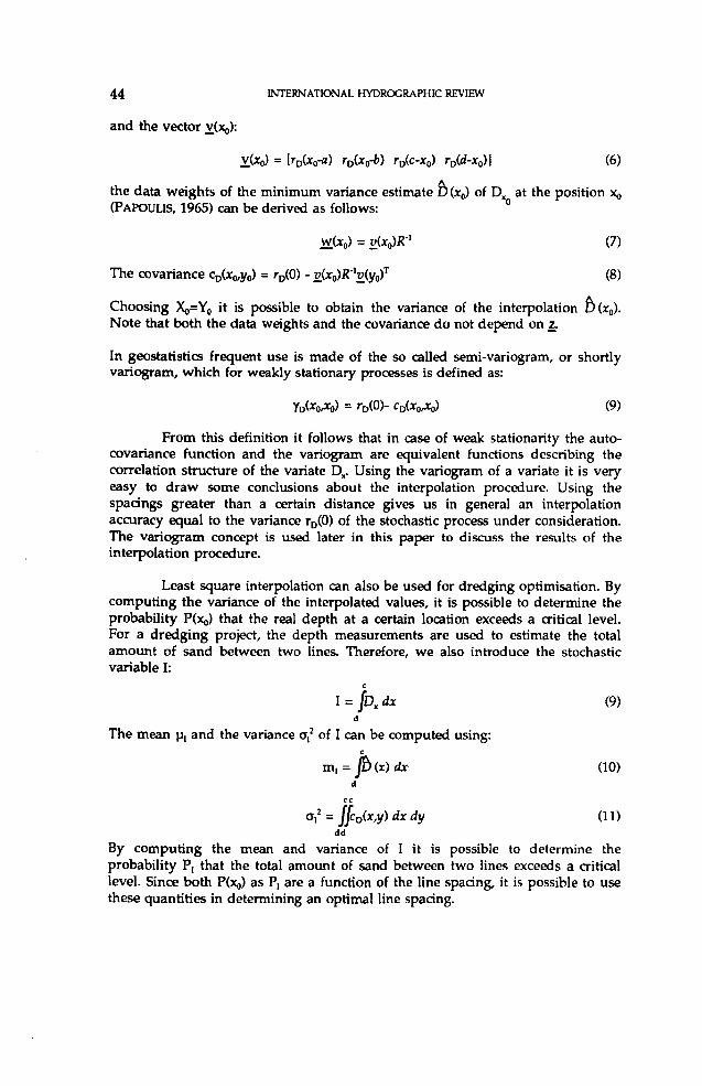
and the vector v(Xo):

v(Xo) = [rD(x0-a) rD(x0-b) rD(c-x0) rD(d-x0)] (6)

the data weights of the minimum variance estimate £) (x0) of Dx at the position x*, (PAPOUUS, 1965) can be derived as follows: 0

w(x0) = v(x0)R'1 (7)

The covariance cD(x0,y0) = rD(0) - v(x0)R lv(y0)T (8)

Choosing X0=Y0 it is possible to obtain the variance of the interpolation b (x 0). Note that both the data weights and the covariance do not depend on z.

In geostatistics frequent use is made of the so called semi-variogram, or shortly variogram, which for weakly stationary processes is defined as:

Yd(*o/*o) = ^ (0 )- Cd( V o) (9)From this definition it follows that in case of weak stationarity the auto­

covariance function and the variogram are equivalent functions describing the correlation structure of the variate D„. Using the variogram of a variate it is very easy to draw some conclusions about the interpolation procedure. Using the spadngs greater than a certain distance gives us in general an interpolation accuracy equal to the variance rD(0) of the stochastic process under consideration. The variogram concept is used later in this paper to discuss the results of the interpolation procedure.

Least square interpolation can also be used for dredging optimisation. By computing the variance of the interpolated values, it is possible to determine the probability P(xo) that the real depth at a certain location exceeds a critical level. For a dredging project, the depth measurements are used to estimate the total amount of sand between two lines. Therefore, we also introduce the stochastic variable I:

dThe mean p, and the variance o,2 of I can be computed using:

c

m, = p (x) dx (10)d

c c

o,2 = ffcD(x,y) dx dy (11)dd

By computing the mean and variance of I it is possible to determine the probability P, that the total amount of sand between two lines exceeds a critical level. Since both P(x0) as P, are a function of the line sparing, it is possible to use these quantities in determining an optimal line sparing.

DISCUSSION

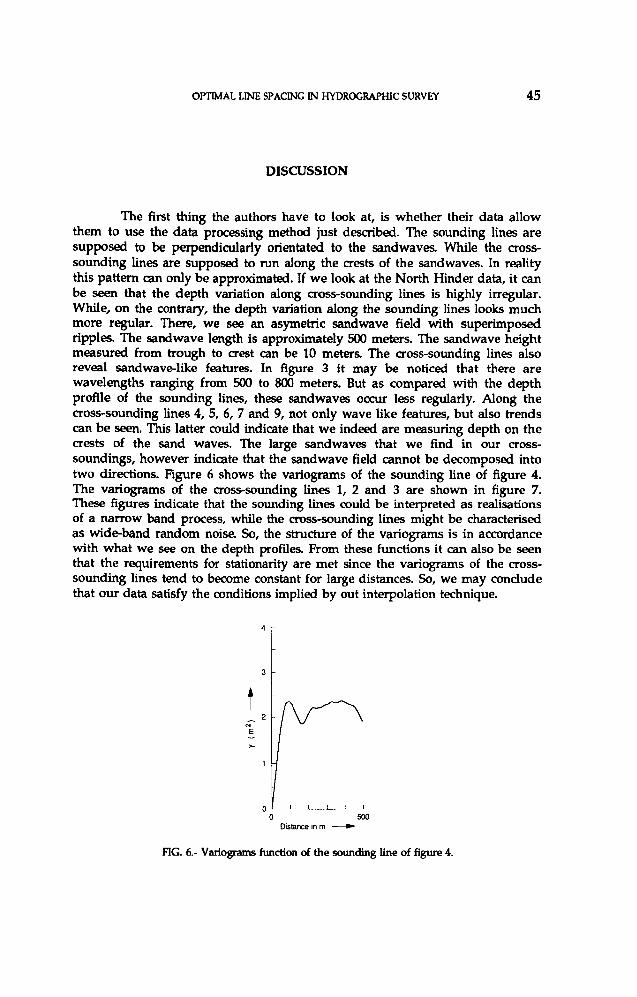
The first thing the authors have to look at, is whether their data allow them to use the data processing method just described. The sounding lines are supposed to be perpendicularly orientated to the sandwaves. While the cross­sounding lines are supposed to run along the crests of the sandwaves. In reality this pattern can only be approximated. If we look at the North Hinder data, it can be seen that the depth variation along cross-sounding lines is highly irregular. While, on the contrary, the depth variation along the sounding lines looks much more regular. There, we see an asymétrie sandwave field with superimposed ripples. The sandwave length is approximately 500 meters. The sandwave height measured from trough to crest can be 10 meters. The cross-sounding lines also reveal sandwave-like features. In figure 3 it may be noticed that there are wavelengths ranging from 500 to 800 meters. But as compared with the depth profile of the sounding lines, these sandwaves occur less regularly. Along the cross-sounding lines 4, 5, 6, 7 and 9, not only wave like features, but also trends can be seen. This latter could indicate that we indeed are measuring depth on the crests of the sand waves. The large sandwaves that we find in our cross­soundings, however indicate that the sandwave field cannot be decomposed into two directions. Figure 6 shows the variograms of the sounding line of figure 4. The variograms of the cross-sounding lines 1, 2 and 3 are shown in figure 7. These figures indicate that the sounding lines could be interpreted as realisations of a narrow band process, while the cross-sounding lines might be characterised as wide-band random noise So, the structure of the variograms is in accordance with what we see on the depth profiles. From these functions it can also be seen that the requirements for stationarity are met since the variograms of the cross­sounding lines tend to become constant for large distances. So, we may conclude that our data satisfy the conditions implied by out interpolation technique.

FIG. 6.- Variograms function of the sounding line of figure 4.

S o u n d in g line 1 Sounding line 2 Sounding line 3

r5 L

FIG. 7.- Variograms function of cross-sounding lines 1, 2 and 3,

Our aim is to obtain a relation between interpolation variance and line spacing. This relation is not unique however, but depends on the sample used to estimate the auto-covariance function. Although the variograms all indicate stationary, it is not true that each of them represents the same bottom structure for large areas. In fact, it appears that each of them only represents the bottom structure in the vicinity of the sample location. So, in deriving relations between line spacing and interpolation variance it must be checked that the sample represents the survey area and that the variograms of the cross-sounding lines do not differ too much in a survey area.

Using the data processing technique as described in this paper, it is necessary that for every calculation a set of four depth values taken from the sounding lines and an auto-covariance function of a cross-sounding line are selected. By selecting the four depth values the line spacing is implicitly set since they are taken from the actual sounding lines. The four sounding lines are not necessarily equidistant in this method. However, the authors have tried to achieve almost equidistancy to simulate actual survey procedures. Then they calculated the maximum interpolation error for the applied line spacing and used auto­correlation function of the cross-sounding line. By varying the line spacing and the used auto- co variance function, pairs of maximum interpolation values and line spacings are obtained. These pairs are plotted in figure 8. The vertical axis of the graphs indicates interpolation errors in meters. Interpolations using cross- sounding line 1 are indicated with straight lines, the ones using cross-sounding line 2 are drawn with a broken line and those using cross-sounding line 3 have dotted lines. On the other har.d, variation of the cross-sounding line while using the same depth values, gives rise to differences in the respective graphs of up to

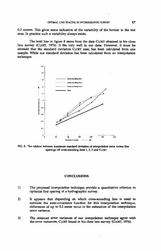
0.2 meters. This gives some indication of the variability of the bottom in the test area. In practice such a variability always exists.

The bold line in figure 8 stems from the data CLOET obtained in his close line survey (CLOET, 1976). It fits very well in our data. However, it must be stressed that the standard deviation CLOET uses, has been calculated from one sample. While our standard deviation has been calculated from an interpolation technique.

2 .° r

1.8 -

1.6 -

1.4 -

1 .2 -

I 1 .0 - |5| 0.8 - SjI® 0 .6 -

0.4

0 .2 '

0 -0 50 100 150 200 250 300

Distance in meters ----------------------►

FIG. 8.- The relation between maximum standard deviation of interpolation error versus line spadngs off cross-sounding lines 1, 2, 3 and CLOET.

CONCLUSIONS

1) The proposed interpolation technique provide a quantitative criterion to optimize line spacing of a hydrographic survey.

2) It appears that depending on which cross-sounding line is used to estimate the auto-covariance function for this interpolation technique, differences of up to 0.2 meter occur in the estimation of the interpolation error variance.

— cross-sounding line 1

■ - cross-sounding line 2

— cross-sounding line 3

3) The obtained error variances of our interpolation technique agree with the error variances, CLOET found in his dose line survey (CLOET, 1976).

Acknowledgements

We greatly appreciate the support of H. Ferwerda of the Hydrographic Service Royal Netherlands Navy for providing us with the unusual cross­sounding lines and J. GROOS of the Tidal Waters Division for assisting us with the computations.

References

Ba st in , G. and G EVERS, M., 1985: Identification and Optimal estimation of Random Fields from Scattered Point-wise Data, Automation Vol. 21, No. 2, pp 139-155.

C h il e s , J.P. and C h a u v et , P., 1975: Kriging: a method for cartography of the sea floor. The International Hydrographic Review, Vol. U l(l), January, pp 25-42.

CLOET, R.L., 1976: The Effect of Line Spacing on Survey Accuracy in a Sand-wave Area, The Hydrographic Journal, Vol. 2.

Delfiner, P., 1975: Linear Estimation of non Stationary Phenomena, Advanced Gcostatistics in the Mining Industry, M. Guarascio et al (eds), D. Reidel Publ. Co. Dordrecht, pp 49-68.

DELHOMME, J.P., 1978: Kriging in the hydroscience, Advances in Water Resources, Vol. 1

MATHERON, G., 1978: The Intrinsic Random Functions and their Applications, Advances Applied Probability, Vol. 5, 439.

P a p o u lis , A., 1965: Probability, Random Variables and Stochastic Processes, Me Graw Hill Kogakusha Ltd., Tokyo.