The Optimal-Location Query

The Optimal-Location Query

Yang Du, Donghui Zhang�, and Tian Xia

College of Computer & Information Science,Northeastern University, Boston, MA 02115

{duy, donghui, tianxia}@ccs.neu.edu

Abstract. We propose and solve the optimal-location query in spatialdatabases. Given a set S of sites, a set O of weighted objects, and aspatial region Q, the optimal-location query returns a location in Q withmaximum influence. Here the influence of a location l is the total weightof its RNNs, i.e. the total weight of objects in O that are closer to l thanto any site in S. This new query has practical applications, but is verychallenging to solve. Existing work on computing RNNs assumes a singlequery location, and thus cannot be used to compute optimal locations.The reason is that there are infinite candidate locations in Q. If wecheck a finite set of candidate locations, the result can be inaccurate,i.e. the revealed location may not have maximum influence. This paperproposes three methods that accurately compute optimal locations. Thefirst method uses a standard R*-tree. To compute an optimal location,the method retrieves certain objects from the R*-tree and sends them asa stream to a plane-sweep algorithm, which uses a new data structurecalled the aSB-tree to ensure query efficiency. The second method isbased on a new index structure called the OL-tree, which novelly extendsthe k-d-B-tree to store segmented rectangular records. The OL-tree isonly of theoretical usage for it is not space efficient. The most practicalapproach is based on a new index structure called the Virtual OL-tree.These methods are theoretically and experimentally evaluated.

1 Introduction

Spatial databases play more and more important roles in applications such ascorporation decision-support systems. For instance, an interesting query thatthe McDonald’s Corporation may ask again and again is: “what is the optimallocation in a given region to put a new McDonald’s store?” Here an optimallocation can be defined as a location which geographically benefits the mostnumber of customers. This example motivates the optimal-location query. Ingeneral, let S be the set of sites (e.g. existing McDonald’s stores) and let O bethe set of weighted objects (e.g. residential buildings, where the weight for abuilding is the number of residents in it). Given a spatial region Q, the optimal-location query computes a location l in Q which maximizes the total weight ofobjects that are closer to l than to any site.

� Supported by NSF CAREER Award IIS-0347600.

C. Bauzer Medeiros et al. (Eds.): SSTD 2005, LNCS 3633, pp. 163–180, 2005.c© Springer-Verlag Berlin Heidelberg 2005

164 Y. Du, D. Zhang, and T. Xia

We focus our discussions on the L1 distance (also known as Manhattan dis-tance) for it more accurately models the driving distance in a city road net-work [SKC93]. Given two locations (x1, y1) and (x2, y2), their L1 distance is|x1 − x2| + |y1 − y2|. If a road network consists of a set of north-south roadsand a set of east-west roads (e.g. in Manhattan), the L1 distance is the shortestdriving distance. When we say “the closest site of o”, we mean the site whoseL1 distance to o is the smallest.

A closely related problem is the bichromatic Reverse Nearest Neighbor (RNN)query [KM00, YL01, SRAE01]. There, a query location is given, and the RNNquery computes the set of objects in O that are closer to l than to any sitein S. There are three differences between the bichromatic RNN query and ournewly proposed optimal-location query. A small difference is that the RNN queryconsiders L2 distance (also known as Euclidean distance). The most importantdifference is that the optimal-location query involves a query region Q, whichconsists of infinite number of candidate locations. One can approximate Q asa grid, and limit the candidates to the finite set of grid intersections. But thisapproach cannot accurately compute optimal locations, for the optimal locationmay be off the grid. The third difference is that the optimal-location query isinterested in the influence of a candidate location, or the total weight of objectsin the RNN set, instead of the RNN objects themselves.

This paper proposes three methods that accurately compute optimal loca-tions. The first solution (Section 4) assumes we have an R*-tree indexing theset O of objects. Similar to how the Rdnn-tree [YL01] extends the R-tree, weassume the R-tree stores some extra information. Every object stores the L1distance to its closest site in S, and every index entry stores the maximum L1distance of objects in the sub-tree. In particular, we propose a concept called thenn buffer, for an object o. It is a spatial contour such that a location l is insideo.nn buffer, if and only if o is closer to l than to any site. As we will see later,each such contour, based on L1 distance, has the shape of a diamond which hasfour right angles. If we rotate the coordinate by 45o counter-clockwise, everynn buffer is an axis-parallel square in the rotated coordinate. The solution fol-lows two steps. The first step is to retrieve from the R*-tree those objects whichmay affect the influence of some locations in Q. The objects are identified incertain order which enables a plane-sweep algorithm (as the second step) to gothrough the stream of objects once and identify an optimal location. The onlyobjects that may affect the influence of locations in the query region Q are theones whose nn buffers intersect with Q. Our approach retrieves such objects inincreasing order of nn buffer.x low in the rotated coordinate, even though theR*-tree was built in the original coordinate. This enables the run-time planesweep. A naive plane-sweep solution has O(n2) cost, where n is the number ofobjects in the stream. We propose the aggregation SB-tree (aSB-tree), extendedfrom the SB-tree [YW01], to reduce the query cost to O(n log n).

Our second solution (Section 5.1) to the optimal-location query is based on anew specialized aggregation index called the OL-tree. It is disk-based, balancedand dynamically updateable. The index is built in the rotated coordinate. It

The Optimal-Location Query 165

is a novel extension to the k-d-B-tree. While the k-d-B-tree maintains pointobjects, the OL-tree keeps axis-parallel squares. In the OL-tree, each index entrymaintains a value called fullcover to count how many squares fully contain therange of it. Besides, Each index entry stores maxoverlap: the maximum localinfluence in the sub-tree, and maxrange, a rectangular region where any locationin it has maximum local influence.

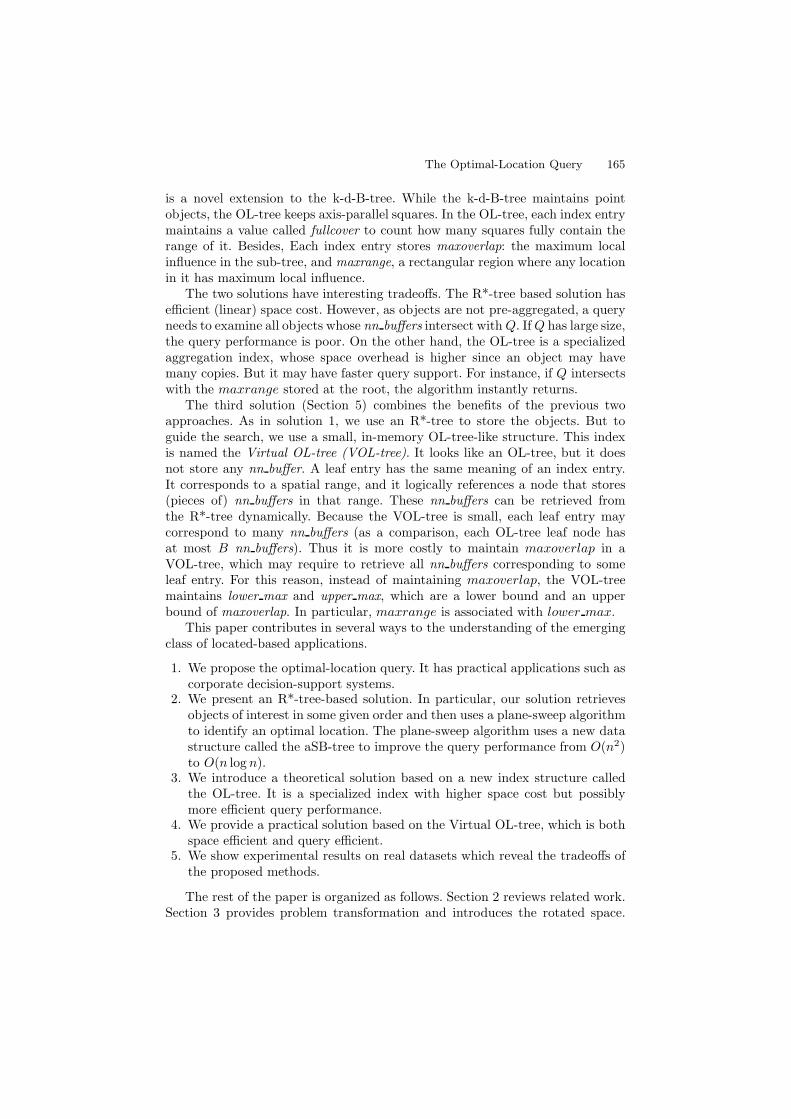
The two solutions have interesting tradeoffs. The R*-tree based solution hasefficient (linear) space cost. However, as objects are not pre-aggregated, a queryneeds to examine all objects whose nn buffers intersect with Q. If Q has large size,the query performance is poor. On the other hand, the OL-tree is a specializedaggregation index, whose space overhead is higher since an object may havemany copies. But it may have faster query support. For instance, if Q intersectswith the maxrange stored at the root, the algorithm instantly returns.

The third solution (Section 5) combines the benefits of the previous twoapproaches. As in solution 1, we use an R*-tree to store the objects. But toguide the search, we use a small, in-memory OL-tree-like structure. This indexis named the Virtual OL-tree (VOL-tree). It looks like an OL-tree, but it doesnot store any nn buffer. A leaf entry has the same meaning of an index entry.It corresponds to a spatial range, and it logically references a node that stores(pieces of) nn buffers in that range. These nn buffers can be retrieved fromthe R*-tree dynamically. Because the VOL-tree is small, each leaf entry maycorrespond to many nn buffers (as a comparison, each OL-tree leaf node hasat most B nn buffers). Thus it is more costly to maintain maxoverlap in aVOL-tree, which may require to retrieve all nn buffers corresponding to someleaf entry. For this reason, instead of maintaining maxoverlap, the VOL-treemaintains lower max and upper max, which are a lower bound and an upperbound of maxoverlap. In particular, maxrange is associated with lower max.

This paper contributes in several ways to the understanding of the emergingclass of located-based applications.

1. We propose the optimal-location query. It has practical applications such ascorporate decision-support systems.

2. We present an R*-tree-based solution. In particular, our solution retrievesobjects of interest in some given order and then uses a plane-sweep algorithmto identify an optimal location. The plane-sweep algorithm uses a new datastructure called the aSB-tree to improve the query performance from O(n2)to O(n log n).

3. We introduce a theoretical solution based on a new index structure calledthe OL-tree. It is a specialized index with higher space cost but possiblymore efficient query performance.

4. We provide a practical solution based on the Virtual OL-tree, which is bothspace efficient and query efficient.

5. We show experimental results on real datasets which reveal the tradeoffs ofthe proposed methods.

The rest of the paper is organized as follows. Section 2 reviews related work.Section 3 provides problem transformation and introduces the rotated space.


Section 4 presents the R*-tree-based solution. Section 5 presents the OL-tree-based and the Virtual-OL-tree-based solutions. Section 7 shows performanceresults. And Section 8 concludes the paper.

2 Related Work

The nearest neighbor (NN) query, since its introduction in [RKV95], has receivedvast attention in spatial database research community. One recent variation in-troduced by [KM00] was the RNN query. That is, given a query location l, findthe objects in a given set O that consider l as their nearest neighbor. Note thatexisting work assumes the Euclidean distance while we focus on the Manhattandistance.

There are two variations of the RNN query: the monochromatic case andthe bichromatic case. In the monochromatic case [SAE00, TPL04], the distancebetween an object o ∈ O and the query location l is compared with the distancesbetween o and other objects in O. In the bichromatic case [SRAE01], there isanother dataset: a set S of sites. And the distance between o and l is comparedwith the distances between o and sites in S. Many real-life applications corre-spond to the bichromatic case. For instance, given a new location, compute theset of residence buildings that are closer to this location than to any existingMcDonald’s store. In [Smi97], it was proved that for the monochromatic case,the number of RNNs is bounded. For instance, there are at most 6 RNNs in the2D case and at most 12 RNNs in the 3D case. But for the bichromatic case, thenumber of RNNs is unbounded even for the 2D case.

One solution to the bichromatic RNN query is based on precomputation[KM00, YL01]. (It also works for the monochromatic case.) The idea of [KM00]is to build an R-tree that stores circles instead of points. Every circle is centeredat some object o, with radius being the distance from o to its nearest site.Precomputation is required to get these distances. Given a query location l, itsRNNs are retrieved by locating the circles that enclose l.

Yang and Lin [YL01] proposed the Rdnn-tree which combines the R-tree ofcircles with the R-tree of objects. It is an R-tree of objects, where every objectstores the distance to its closest site, while every index entry stores the maximumdistance of all objects in the sub-tree. The structure logically maintains the R-tree of circles. It remains to determine, given a location l and an index entrye, whether the sub-tree referenced by e may contain some object whose “circle”(not stored) encloses l. The solution is to expand the index entry’s MBR outwardby the associated maximum distance. If the expanded region does not enclose l,there is no need to check the sub-tree.

The R-tree that we use, in the first solution to the optimal-location query,is the Rdnn-tree [YL01] which stores L1 distance instead of L2 distance. Ourconcept of nn buffer corresponds to their concept of circle for each object. How-ever, in this paper both the addressed problem and the R-tree-based solutionare different from [YL01]. Our problem takes as input a spatial region and aimsat identifying an optimal location (with maximum influence), while [YL01] takes


as input a single location and finds its RNNs. As for the solution, while [YL01]finds the objects whose circles enclose the given location and terminates, we findthe objects whose nn buffers intersects with the given region as the first stageof a pipeline process. The second pipeline stage takes this stream of objects andidentifies an optimal location via plane sweep.

Another bichromatic RNN query solution was proposed by [SRAE01]. Theidea is to dynamically construct the influence region of the query location l. Here,the influence region is defined as a polygon in space which encloses and onlyencloses all possible RNNs of l. This is equivalent to the Voronoi cell enclosingl [BKOS97]. Conceptually, if we draw a bisector line between l and a site s, anyobject located on the l side of the bisector will have smaller Euclidean distanceto l than to s. The l side of the bisector is a half plane. If we compare l againstall sites and take the intersection of these l-side half planes, we get the Voronoicell containing l.

Of course, to compare with all sites is expensive. [SRAE01] provides a cleverway to compute the rectangle that is guaranteed to contain all sites needed forcomputing the exact Voronoi cell of l. Then the Voronoi cell of l can be computedby only examining these sites with in the rectangle. So to find the RNNs of l, arange query using the Voronoi cell is performed on the R-tree of objects.

If we had limited candidate locations, the approach could be extended tosolve the optimal location problem, with two modifications. First, we now needto construct a Voronoi cell with regards to the L1 distance [LW80]. Second,for each location, we need to know its influence rather than the actual RNNobjects. So we can index the set of objects using the aggregation R-tree (aR-tree) [PKZT01] where each index entry stores the total weight of objects in thesub-tree. If the MBR of an index entry is contained in a Voronoi cell, the storedtotal weight contributes to the computation of influence, without browsing thesub-tree.

Unfortunately, in the optimal-location query, there are infinite number ofcandidate locations. So the approach of [SRAE01] (with the above modifica-tions) does not work. Before presenting our solutions, let’s first study a problemreduction.

3 Problem Transformation

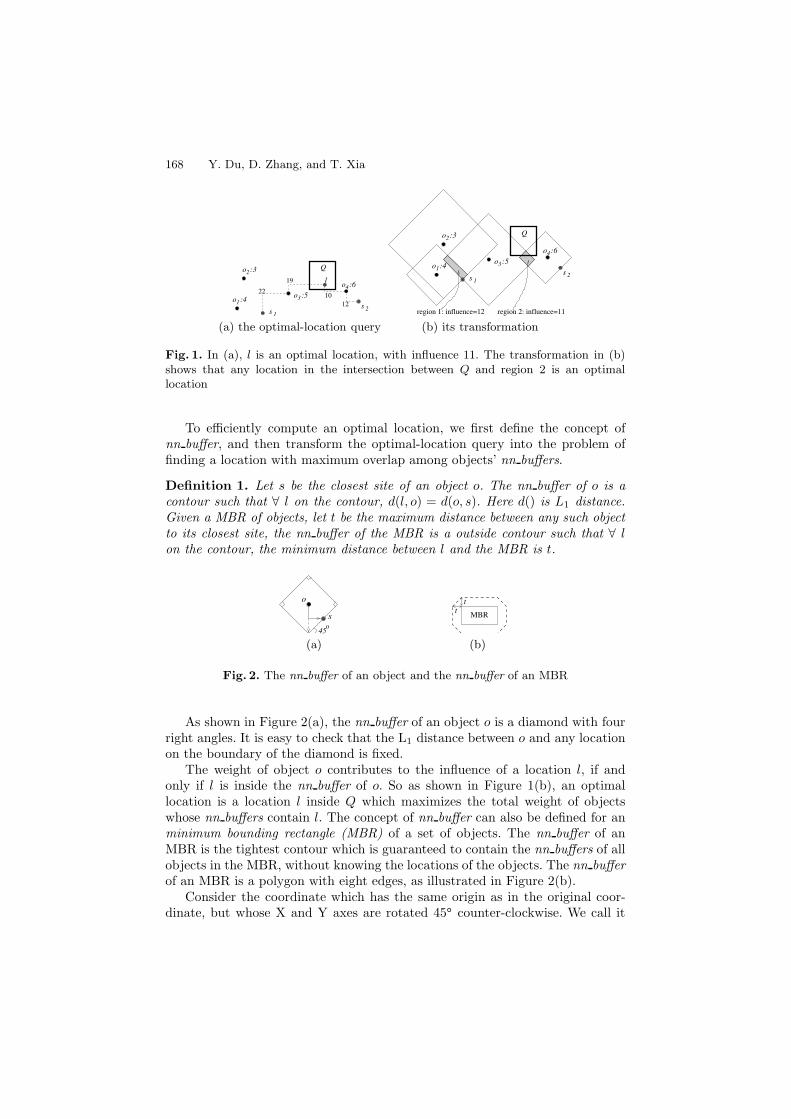
An illustration of the optimal-location query, defined in Section 1, appears inFigure 1(a). There are four objects and two sites. In particular, the object o3with weight 5 has s1 as the closest site, where d(o3, s1)=22. And the object o4with weight 6 has s2 as the closest site, where d(o4, s2)=12. The influence of alocation is the total weight of objects that are closer to this location than totheir closest sites. For instance, the influence of l is the total weight of o3 ando4, which is 5+6=11. Given a query region Q, the optimal-location query findsan location inside Q with maximum influence. In this example, l is an optimallocation. There may be more than one optimal location. The query asks for oneof them.


l

1s 2

o :3 2

o :4 1 o :5 3

o :6 4

1210

s

Q

19

22

region 2: influence=11region 1: influence=12

o :4 1

o :3 2

o :5 3

o :6 4

s

Q

1s 2

(a) the optimal-location query (b) its transformation

Fig. 1. In (a), l is an optimal location, with influence 11. The transformation in (b)shows that any location in the intersection between Q and region 2 is an optimallocation

To efficiently compute an optimal location, we first define the concept ofnn buffer, and then transform the optimal-location query into the problem offinding a location with maximum overlap among objects’ nn buffers.

Definition 1. Let s be the closest site of an object o. The nn buffer of o is acontour such that ∀ l on the contour, d(l, o) = d(o, s). Here d() is L1 distance.Given a MBR of objects, let t be the maximum distance between any such objectto its closest site, the nn buffer of the MBR is a outside contour such that ∀ lon the contour, the minimum distance between l and the MBR is t.

o

45

so

MBRtt

(a) (b)

Fig. 2. The nn buffer of an object and the nn buffer of an MBR

As shown in Figure 2(a), the nn buffer of an object o is a diamond with fourright angles. It is easy to check that the L1 distance between o and any locationon the boundary of the diamond is fixed.

The weight of object o contributes to the influence of a location l, if andonly if l is inside the nn buffer of o. So as shown in Figure 1(b), an optimallocation is a location l inside Q which maximizes the total weight of objectswhose nn buffers contain l. The concept of nn buffer can also be defined for anminimum bounding rectangle (MBR) of a set of objects. The nn buffer of anMBR is the tightest contour which is guaranteed to contain the nn buffers of allobjects in the MBR, without knowing the locations of the objects. The nn bufferof an MBR is a polygon with eight edges, as illustrated in Figure 2(b).

Consider the coordinate which has the same origin as in the original coor-dinate, but whose X and Y axes are rotated 45o counter-clockwise. We call it


the 45o (reads rotate-45-degree) coordinate (Figure 3). In this paper, the R*-tree indexes in the original coordinate (to satisfy the possible need for otherapplications), while the aSB-tree, the OL-tree and the VOL-tree indexes in the

45o coordinate.

t

45o

oX’

X

Y

Y’

x

yx’

y’

Fig. 3. Illustration of the ro-tated coordinate

Our analysis shows that an object o locatedat (x, y) in the original coordinate is mappedto (x+y√

2, −x+y√

2) in the 45o coordinate. Fur-

thermore, let t be the L1 distance from o toits closest site. The nn buffer of o is an axis-parallel square in the 45o coordinate, whoselower-left corner and upper-right corner are:(x+y−t√

2, −x+y−t√

2) and (x+y+t√

2, −x+y+t√

2).

4 The R*-Tree-Based Solution

Our first solution to the optimal-location query assumes the objects are indexedby an R*-tree. Similar to how the Rdnn-tree [YL01] extends the R*-tree, weassume every object stores the L1 distance to its closest site, and every indexentry stores the maximum L1 distance of objects in the sub-tree.

The R*-tree indexes objects in the original coordinate (not the 45o coor-dinate), since there may be other applications that need to access the data inthe original coordinate. However the plane-sweep algorithm works in the 45o

coordinate. In order to do the plain sweep, we have to retrieve the objects inincreasing order of their nn buffer’s x low in the 45o coordinate. Section 4.1shows how to retrieve objects, Section 4.2 describe a naive plane sweep algorithmwith O(n2) cost, Section 4.3 propose the aSB-tree structure which can reducethe worst-case query cost to O(n log n), and Section 4.4 extends the algorithmsto incorporate a rotated query region.

4.1 Retrieving Objects from the R*-Tree

To retrieve the objects whose nn buffers intersects with Q, we can browse the R*-tree in a top-down fashion, similar to the range query. The difference is that todetermine whether to expand an sub-tree, instead of checking whether its MBRintersects with Q, we check whether the MBR’s nn buffer intersects with Q.

The remaining issue of object retrieval is how to return objects in increasingorder of their nn buffer’s x low in the 45o coordinate. This is achieved by usinga best-first search. That is, we keep a heap of the R*-tree’s index entries aswell as objects. The entries are ordered in increasing nn buffer.x low in the 45o

coordinate. Initially, the heap contains the index entry referencing the wholetree. In each iteration, the entry e with minimum nn buffer.x low is extracted.


If e is a object, output it (to be sent, as the next element of an input stream,to the plane-sweep algorithm discussed in the next section). Otherwise, e is anindex entry. We examine every entry se in the node referenced by e, and pushse into the heap if its nn buffer intersects with Q.

4.2 The Naive Plane Sweep

X

1

o :3 2

o :5 3

o :6 4

12105421 912

5

89

12

Y

o :4

Fig. 4. nn buffers in the rotatedcoordinate

In the rotated coordinate, the nn buffers areaxis-parallel squares. To find the optimal lo-cation, the basic idea is to perform a planesweep in increasing order of X . For eachparticular X , the Y axis is partitioned intoa set of intervals, each associated with aninfluence value. For instance, at X=4, theY axis is partitioned into six intervals: (-∞,2):0, (2,5):5, (5,8):12, (8,9):7, (9,12):3, and(12,∞):0. Whenever a change happens, up-date the set of intervals. During the process,always maintain a location with maximum in-fluence. In fact we can maintain a rectangularregion with maximum influence, instead of asingle location.

At the end, any location in the maintained region is an optimal location. Asan example, in Figure 4, any location in the X range of (4,5) and Y range of(5,8) is an optimal location, with influence 12.

4.3 The aSB-Tree

The naive plane sweep has O(n2) worst-case performance. The reason is thatthere are O(n) events to handle, and each event needs to scan through O(n)intervals that partition the Y axis. We hereby propose a data structure calledthe Aggregation SB-tree (aSB-tree), derived from the SB-tree [YW01]. The newstructure enables any event to be processed in O(log n) time, and thereforereduces the overall cost to O(n log n).

The idea is to organize the intervals (that partition the Y axis) into a bal-anced B-tree-like structure. To insert a new Y range which may affect manyintervals in the naive approach, with the aSB-tree we only need to update twopaths from root to leaf. The key idea that enables this is: if the Y range to beinserted fully contains the interval of an index entry, we do not insert into thesub-tree. Instead, we update a value fullcover maintained along with the indexentry. The aSB-tree extends the SB-tree by storing the max influence and thecorresponding spatial region in the sub-tree. Figure 5 shows a two-level aSB-tree,which corresponds to Figure 4 right after processing the event at X = 4 and theevent at X = 5. Let’s examine it in more details.


and Y in (5, 8)

(−M, 2): 0 (2, 5): 5 (5, 8): 12 (8, 9): 7 (9, 12): 3 (12, M): 0

max=3 in (9, 12) at X>2max=5 in (2, 5) at X>4

(−M, 5): 0 (9, M): 0

(−M, M): 0root entry:

Global max = 12max=12 in (5, 8) at X>4

max=12 in (5, 8) at X>4

(5, 9): 0when X in (4, ?)

(a) at the sweep line X=4

(−M, 2): 0 (2, 5): 5 (5, 8): 12 (8, 9): 7 (9, 12): 3 (12, M): 0

max=3 in (9, 12) at X>2max=5 in (2, 5) at X>4

(−M, 5): 0 (9, M): 0(5, 9): −4

(−M, M): 0max=8 in (5, 8) at X>5

max=12 in (5, 8) at X>5

root entry:

Global max = 12when X in (4, 5) and Y in (5, 8)

(b) at the sweep line X=5

Fig. 5. An example of aSB-tree

Properties inherited from the SB-tree:

– The aSB-tree is a balanced tree structure. The maximum number of entriesin a (leaf or index) node is fixed. Except the root, every node must be atleast half full.

– Every entry corresponds to an interval (a Y range). For any index entry e,all intervals of entries in Node(e) form an exact partition of e.interval. E.g.in Figure 5(a), the root entry has an interval as the whole Y space.

– Every leaf entry has a value influence. In Figure 5(a), the leaf entry (5,8):12means that right after the current X = 4, any location with Y ∈ (5, 8) hasinfluence 12.

– Every index entry has a value fullcover, which corresponds to the total weightof inserted Y ranges which fully cover the entry’s interval. E.g. the secondindex entry in the root of Figure 5(a), which has (5,9):0, means its fullcoveris 0, while the interval is (5,9).

– To insert a range I with weight w, we update (at most) two paths from theroot to the leaf level. These are the nodes whose referencing entry’s intervalpartially intersects with I. E.g. Figure 5(b) shows the result after processingthe event at X = 5, i.e. inserting I=(5,9) and w=-4. In particular, theinsertion stopped at the root node, since no entry in the root node has aninterval partially intersecting with I. For any entry (e.g. the second indexentry in root) whose interval is contained in I, w is added to its fullcover.An overflow/underflow, if happens, is treated like in the B-tree.

Properties extended from the SB-tree:

– There is a gap between what the SB-tree provides and what we need. Theultimate goal we need is: after all the nn buffers are seen, report an optimallocation with its influence. To do so, separate from the aSB-tree we maintaina globally maximum influence and its spatial range.


– This global max is maintained after processing each insertion. Here everyindex entry in the aSB-tree stores the local maximum influence of some lo-cation in the sub-tree. It is local because the actual influence should consistsof the fullcover of index entries for all ancestor nodes. For instance, in thesecond index entry in Figure 5(b), the local maximum influence is 12. Butthe actual maximum influence is 12+(-4)=8. Since the old global max is nosmaller than the new one, it is not changed.

– Along with each local maximum influence stored at an index entry, or withthe global max, we also store the corresponding spatial region. That is, anylocation in this region has this maximum influence. For a local max, itscorresponding region only needs to store the left X border for the rightborder is not known yet. With a new insertion, it is possible to close the rightborder of the previous max region and start a new one. E.g. in Figure 5(b),two index entries’ local max region change their left border from X = 4 toX = 5. The right border of the global max region may need to be closedcorrespondingly. All the additional information can be maintained along withthe insertion process, by following the insertion paths backwards. So theupdate cost remains O(log n) as in the SB-tree. Therefore, the plane-sweepalgorithm integrated with the aSB-tree has O(n log n) query cost.

4.4 Extension to Involve a Query Region

In the original coordinate, the query region Q is an axis-parallel rectangle. Thus,in the 45o coordinate, the query region Q becomes a rectangle rotated 45o clock-wise (as shown in Figure 6). To perform the query correctly, our aSB-tree basedplane-sweep algorithm needs to be extended as follows:

– The Y space of the aSB-tree is not the wholespace (-M ,M), but the Y projection of Q.This is because we only care about the loca-tions in Q. In Figure 6, the Y space of theaSB-tree should be (yl, yh).

– For each nn buffer, we calculate the smallestX (called start) when it ‘enters’ Q and thelargest X (called end) when it ‘leaves’ Q.The insertion/removal events occur at thesecalculated X values, instead of the x low andx high of the nn buffers.

h

yl

endstart X

Yy

Q

Fig. 6. Illustration of a ro-tated query region

– Finally, it is no longer true that whenever the aSB-tree is updated due to anevent, the current maximum influence is known only by checking the rootentry. The reason is that the maintained maximum influence may be in aregion outside Q. To address this issue, we perform a range-max query onthe aSB-tree. That is to find the maximum influence within the actual Yrange. The range-max query can be performed in O(log n) time, since it onlyneeds to examine two paths of the aSB-tree. The reason is that, similar to


the insertion algorithm, a sub-tree whose interval is contained in the queryinterval does not need to be expanded.

A side note is: even though we use the aSB-tree as an in-memory structureto improve the plain sweep, if needed the structure can be implemented as adisk-based index like the SB-tree.

5 The Virtual OL-Tree

The R*-tree based solution examines all objects whose nn buffers intersect withthe query region Q, and thus is not efficient when a large Q results in theexamination of many objects. This section first proposes an theoretical solutionto the optimal-location query based on a new index structure called the Optimal-Location Tree (OL-tree). Then we extend it to a more practical and efficientsolution based on the Virtual Optimal-Location Tree (VOL-tree).

5.1 The OL-Tree-Based Solution

The OL-tree is a k-d-B-tree-like structure which is balanced, disk-based anddynamically-updateable. Roughly speaking, it stores the nn buffers in the 45o

coordinate. Like the k-d-B-tree, the OL-tree is a space-partitioning method (ver-sus a data-partitioning method like the R*-tree). Unlike the k-d-B-tree, the OL-tree stores rectangular records in its leaf nodes. If a square partially intersectswith the ranges of multiple index entries, it is split and multiple copies are in-serted. However, if the square fully contains the range of some index entry, weonly update a value called fullcover stored along with the index entry, with-out further inserting into the sub-tree. Each index entry stores maxoverlap: themaximum local influence in the sub-tree. That is, the maximum influence in thesub-tree, subtracted by the fullcover values of all ancestor index entries. A rect-angular region maxrange is also stored, where any location in it has maximumlocal influence. Due to the space limitation, we skip the details of the updateand query processing.

The OL-tree may cause cascading split of child nodes if splitting an indexnode. One may wonder how bad the space complexity can be. We argue that thespace complexity of the OL-tree (with an additional requirement) is O(n2/B)for the following reasons. First, the total number of leaf entries is O(n2). With naxis-parallel squares, there are O(n) different X positions and O(n) different Ypositions, which form O(n2) cells. In the worse case each cell is stored in the treeseparately. Thus there are at most O(n2) leaf entries. Second, the total numberof nodes in O(n2/B). The linear storage of the k-d-B-tree can be guaranteedby re-organization of sub-trees which contain too few leaf entries. Similarly, theOL-tree with O(n2) leaf entries needs O(n2/B) nodes.

This bound reveals that the OL-tree is not a practical spatial index structure.In the next subsection we introduce a practical structure, named the VOL-tree,to solve the optimal-location query.


5.2 The VOL-Tree Structure

The OL-tree has more than linear space because if an nn buffer is split intomultiple pieces, each of them is physically stored in some leaf node(s). What ifwe do not physically store any leaf node of the OL-tree? We can use an R*-treeto store the original objects, and whenever the content of a leaf node is needed,we perform a range query on the R*-tree. This is the key idea to the VirtualOL-tree (VOL-tree).

It is challenging to implement this idea. As we already spend the space tostore the R*-tree, it is ideal to have a small VOL-tree that fits in memory. On theother hand, as there are O(n2/B) leaf nodes in an OL-tree, there are O(n2/B2)index nodes, which would be the size of the VOL-tree if we treat it as an OL-tree without leaf nodes. There is a big gap. Thus we claim that the VOL-tree isNOT merely an OL-tree without the leaf level. It has to be much much smaller,possibly only consisting of one index level besides the root. A consequence is thateach leaf entry of the VOL-tree corresponds to a virtual node (content stored inthe R*-tree) with much more than B nn buffers. So a crucial issue jumps out: itis expensive to maintain maxrange and maxoverlap because an update requiresus to perform plane sweeps on the virtual nodes.

To address this issue, we propose another change from the OL-tree: alongwith each index entry, instead of keeping the accurate maxoverlap, keep twovalues lowermax and uppermax, which are a lower bound and an upper boundof maxoverlap.

In more detail, the entries in the tree are as follows:

– An index entry e has the following format: (range, nodeID, fullcover,lowermax, maxrange, uppermax). Here range is the spatial range of thecorresponding sub-tree, and nodeID points to the referenced node. The valuefullcover is the total weight of nn buffers whose insertion stopped at e (sucha nn buffer contains e.range, but not the range of e’s parent).

– The values lowermax and uppermax are some lower and upper bounds ofthe maximum local influence in e.range. And maxrange is a rectangle fullycontained in e.range where every location in maxrange has local influence= lowermax.

– A leaf entry and an index entry have the same content, with a minor differ-ence that a leaf entry’s nodeID is empty.

5.3 The VOL-Tree Query Algorithm

Figure 7 shows the optimal-location-query algorithm in the VOL-tree. We startfrom the root node. In the VOL-tree, even if root.maxrange intersects with Q, itis possible that some location in Q−root.maxrange has an influence larger thanroot.lowermax (when root.lowermax < root.uppermax). So as Step 1 shows,we can safely return a location in root.maxrange ∩ Q only if root.lowermax =root.uppermax or Q is completely inside root.maxrange.

Step 2 inserts the root entry into a heap. Every entry in the heap has, besidesan index entry, two values min and upper. These are the actual ( not local) lower


Algorithm. VOLTreeQueryInput: Query region Q, VOL-tree root.Return: An optimal location in Q.

1. if root.maxrange ∩ Q �= ∅ and (root.lowermax = root.uppermax or Q ⊆root.maxrange), return any location in root.maxrange ∩ Q.

2. heap.Insert(root, 0, root.uppermax)3. Set opt loc as an arbitrary location in Q, and opt inf = 0,4. while heap is not empty

(a) (e, min, upper) = heap.ExtractMaxUpper().(b) if upper ≤ opt inf , return opt loc.(c) if e references an index node

for every entry se in Node(e.nodeID) s.t. se.range ∩ Q �= ∅A. Set m = min + se.fullcover, and u = min + se.fullcover +

se.uppermax.B. if u ≤ opt inf , goto next entry.C. if opt inf < m, set opt inf = m and opt loc be any location in

se.range ∩ Q.D. if se.maxrange ∩ Q �= ∅,

(i) l = min + se.fullcover + se.lowermax(ii) if opt inf < l, set opt inf = l and opt loc be any location in

se.maxrange ∩ Q.(iii) if u �= l and (Q ∩ se.range) � se.maxrange, heap.Insert(se, m, u)

E. elseheap.Insert(se, m, u)

F. end ifend for

(d) elseA. Using e.range ∩ Q as a new query region, retrieve nn buffers from the

R*-tree of objects. Use plane sweep to find an optimal location (inf, loc)within the new query region.

B. if opt inf < min + inf , set opt loc = loc, and opt inf = min + inf .(e) end if

5. end while6. return opt loc.

Fig. 7. Finding an optimal location using the VOL-tree

bound and upper bound of influence for locations in the sub-tree. Meanwhile,we maintain the currently seen optimal location opt loc along with its influenceopt inf , initialized to be an arbitrary location with influence 0 (Step 3).

While the heap is not empty, we process each element at a time. In eachiteration, the heap entry with maximum upper is extracted. As Step 4(b) ofthe algorithm shows, if this extracted upper is no larger than opt inf , we candetermine that opt loc is an optimal location and thus the algorithm returns.The crucial steps are Step 4(c) which expands an index node and Step 4(d)which expands a leaf node.

To expand an index node, we examine every child entry se whose rangeintersects with Q, and try to push se.nodeID into the heap. Here the new lowerbound is m = min + se.fullcover, and the new upper bound is u = min +se.fullcover + se.lowermax. There are two pruning opportunities. First, if thenew upper bound u is no larger than opt inf , there is no need to expand the sub-tree (Step 4(c)B). Second, if se.maxrange intersects with Q, we already know


the influence of the locations within the intersection, and thus we may have thechance to update the maintained optimal location before expanding the sub-tree(Step 4(c)D). It likely causes other entries to be pruned earlier.

To expand a leaf node (Step 4(d)), we go to the R*-tree to retrieve thenn buffers that intersect with e.range∩Q and then perform a plane sweep tech-nique of Section 4 to compute a location inside Q with maximum global influenceinf . If this influence is bigger than opt inf , we update the maintained opt infand opt loc.

5.4 The Update Algorithm

The VOL-tree can be bulk-loaded. Due to space limitations, the algorithm isomitted. We only point out that immediately after bulk-loading, every entryin the VOL-tree has accurate local maximum information, i.e. lowermax =uppermax. With dynamic update, this may not be true. Let us examine theupdate algorithm below.

The insertion algorithm is shown in Figure 8, while a deletion is treated as aninsertion with negative weight. To insert into an index node (Step 1), we considerevery child entry se whose range intersects with the parameter R. If se.range iscontained in R, we simply add w to se.fullcover. If se.range partially intersectswith R, we recursively insert into the sub-tree referenced by se. After insertion,we need to re-aggregate the lowermax, uppermax and maxrange if necessary.

When e refers to a virtual leaf node which is not stored, the actual objectis maintained in a separate R*-tree. So we only need to modify e.lowermax,e.uppermax and e.maxrange. The update of e.uppermax is simple. As Step2(a) shows, for a positive weight, e.uppermax is increased by w. For a negativeweight, e.uppermax remains unchanged. We may modify e.lowermax and/ore.maxrange only if e.maxrange intersects with R. For a positive weight (Step2(c)), the intersection part of e.maxrange and R is the new e.maxrange, withweight increased by w. For a negative weight (Step 2(d)), there are two cases.If e.maxrange is fully covered by R, we decrease e.lowermax. Otherwise, weshrink e.maxrange to e.maxrange − R but keep e.lowermax unchanged.

6 Performance

In this section, we report experimental results on the R*-tree approach and theVOL-tree approach. In our experiments we used real datasets: the Digital Chartof the World from the R-tree Portal [The03]. It contains two type of point data:the populated places and cultural landmarks in North America, a total of 24,493and 9,203 points respectively. We use the populated places as the objects andcultural landmarks as the sites. From the dataset, we generated an object R*-tree for all populated place, which is augmented by the L1 distance from eachobject to its nearest site. We set the page size to 1k and the default buffer sizeto 256 pages. All the programs were written in Java and run on a Pentium IVDell PC equipped with 3.2GHz CPU.


Algorithm. VOLTreeInsertInput: Range R, Weight w, VOL-tree index entry e.Pre-condition: R intersects with, but does not fully contain, e.range.Action: Insert range R with weight w to the sub-tree referenced by e.

1. if e refers to a node in the VOL-tree(a) for every se in Node(e) s.t. R contains se.range, se.fullcover += w.(b) for every se in Node(e) s.t. R partially intersects with se.range,

VOLTreeInsert(R, w, se).(c) Let se0 be the entry in Node(e) with maximum se.fullcover+se.lowermax.(d) Set e.maxrange = se0.maxrange and e.lowermax = se0.fullcover +

se0.lowermax.(e) e.uppermax=max{se.fullcover+se.uppermax} for all entry se in Node(e).

2. else /* e refers to a virtual leaf node */(a) if w > 0, e.uppermax += w.(b) if e.maxrange ∩ R = ∅, return.(c) if w > 0

i. e.maxrange = e.maxrange ∩ Rii. e.lowermax+ = w

(d) elsei. if e.maxrange ⊆ R, e.lowermax+ = w.ii. else e.maxrange = e.maxrange − R.

(e) end if3. end if

Fig. 8. The Insertion algorithm of the VOL-tree

From our preliminary experimental results, we found that it does not helpto make the VOL-tree disk based. So the VOL-tree is in memory, and only theI/O of R*-tree will be measured. However, it consumes part of the buffer. Forexample, if the size of the VOL-tree is 50 pages, the buffer available to the R*-tree retrieval in the VOL-tree based method should be 256− 50 = 206. For eachexperiment we start with a clean buffer, run 100 random queries, and measurethe total I/Os. Buffer will not be flushed during the execution of 100 queries.Our preliminary experimental results show that, with fixed area of the queryrange, the shape of the query range has little impact on the query performanceof the VOL-tree based methods. Thus we always use square query ranges.

In many applications, the datasets are known in advance. For instance, the setof McDonald’s stores and the set of residential buildings can be given in advancewhen building the index, although changes may happen later on. Therefore, weuse the VOL-tree based method with high bulk-loading percentage (80% and100%). In the experiments, we compare the performance of three methods listedin Table 1.

Table 1. There different settings for experiments

Name of method ExplanationR* R*-tree based method (without using VOL-tree)

VOL80 VOL-tree based method with 80% of the objects being bulk loadedVOL100 VOL-tree based method with 100% of the objects being bulk loaded


Fig. 9. The I/O performance ofthe VOL-tree for various size

To utilize the VOL-tree, the first questionto answer is how large the VOL-tree shouldbe. Figure 9 shows the I/O of the R*-tree ofvarious sizes (in the unit of the page size).When the size of the VOL-tree is small(< 20 pages), the I/Os become close to theR*-tree based method (which correspondsto VOL-tree size = 0). When the size of theVOL-tree is large (> 80 pages), the I/Osalso increase. That is because the largerVOL-tree does not help much to prune thesearch space, but it uses a large proportionof the buffer, which results in the worse I/Oof the R*-tree.

From the results, we draw the conclusion that a small VOL-tree is sufficient.Thus, in the later experiments, we set the size of VOL-tree to 20 pages.

To study the effect of the size of query range on the I/Os, we change thearea of the query range. Figure 10 (a) and (b) shows the results when the queryrange is small and is large respectively. When the query area is smaller than1% of the whole space, their performances are very close although VOL-treemethods outperform. When the query area is larger than 1%, the R*-tree basedmethod has I/Os of more than 10,000 so we do not even show it in figure. Anexpected fact is that when the query range becomes very large, the performanceof both VOL80 and VOL100 improve. That is because, the large query rangesis more likely to intersect with maxranges stored in the VOL-tree, and thus ismore likely to prune some subtrees.

(a) Queries with small area (b) Queries with large area

Fig. 10. The I/O performance of of the VOL-tree for various query area

The updates increase the difference between lowermax (uppermax) and thelocal maximal influence, thus decreasing the pruning capability. Figure 11 showshow updates affect the I/O performance. We bulk load some objects and insertthe others. The X-axis presents the percentage of the number of inserted objectsto the number of bulk loaded objects. For example, X = 50% corresponds to the


case when we bulk load 2/3 of the objects and insert the remaining 1/3. Withthe increase of the percentage, the I/O performance decreases. After about 50%insertions, the performance becomes comparable to the R*-tree based method.There are two reasons for that. First, the VOL-tree uses some buffer of the R*-tree. Second, the VOL-tree may cause multiple scans of same page. We need topoint out that even if an application is update intensive, the VOL-tree basedmethod is still a good choice since the tree can be rebuilt in part or in full. Andthe rebuilding cost is amortized. Furthermore, the rebuilding can be integratedwith the query processing.

Fig. 11. The Effect of the Updates Fig. 12. The Effect of the Buffer Size

Figure 12 shows how the buffer size affects the I/O performance of the VOL-tree. When buffer size is 128, the R* outperforms VOL80. That is because theVOL-tree has size of 20 and occupies about 20% the buffer. After the buffersize is doubled to 256, the I/O of VOL80 dramatically drops to below R*. Withthe increase of the buffer size, the performance of all the three methods getimproved, while the VOL-tree based method is again better.

7 Conclusions

In this paper we proposed and solved the optimal-location query. The queryhas real applications, e.g. in corporate decision-support systems. We presentedthree solutions to accurately answer such a query. In particular, the VOL-treeapproach is the most efficient. The approach uses an R*-tree to index the objects,while a small, in-memory VOL-tree is used to prune the search space. The queryperformance is much better than the plain R*-tree approach, especially whenthe query size is large. (Notice that the R*-tree approach is already optimizedvia a new index called the aSB-tree.) For instance, if the query area is 5% of thespace, the VOL-tree approach computes an optimal location 6 times faster thanthe R*-tree approach. If the query size increases, the improvement increasesas well, which can be multiple orders of magnitude better. Also, the size ofthe VOL-tree is small. In our experiments, while the R*-tree of objects is over700 disk pages, the VOL-tree is only 20 pages. The VOL-tree has very efficientupdates, as the index is small and updating it does not need to touch the R*-tree(except for ordinary object insertion/removal). One set of experiments showed


that within 50% new updates, the VOL-tree approach remained to have betterquery performance. Of course, if there are too many updates, the VOL-tree canbe re-built and the cost is amortized across all the new updates. In summary, theVOL-tree approach is the most efficient solution to the optimal-location query.

References

[BKOS97] M. de Berg, M. van Kreveld, M. Overmars, and O. Schwarzkopf. Compu-tational Geometry: Algorithms and Applications. Sprinter Verlag, 1997.

[KM00] F. Korn and S. Muthukrishnan. Influence Sets Based on Reverse NearestNeighbor Queries. In SIGMOD, pages 201–212, 2000.

[LW80] D. T. Lee and C. K. Wong. Voronoi Diagram in L1 (L∞) Metrics with2-Dimensional Storage Applications. SIAM Journal on Computing, 9:200–211, 1980.

[PKZT01] D. Papadias, P. Kalnis, J. Zhang, and Y. Tao. Efficient OLAP Operationsin Spatial Data Warehouses. In SSTD, pages 443–459, 2001.

[RKV95] N. Roussopoulos, S. Kelley, and F. Vincent. Nearest Neighbor Queries. InSIGMOD, pages 71–79, 1995.

[SAE00] I. Stanoi, D. Agrawal, and A. El Abbadi. Reverse Nearest Neighbor Queriesfor Dynamic Databases. In ACM/SIGMOD Int. Workshop on ResearchIssues on Data Mining and Knowledge Discovery (DMKD), pages 44–53,2000.

[SKC93] S. Shekhar, A. Kohli, and M. Coyle. Path Computation Algorithms forAdvanced Traveller Information System (ATIS). In ICDE, pages 31–39,1993.

[Smi97] M. Smid. Closest Point Problems in Computational Geometry. In J.-R. Sack and J. Urrutia, editors, Handbook on Computational Geometry.Elsevier Science Publishing, 1997.

[SRAE01] I. Stanoi, M. Riedewald, D. Agrawal, and A. El Abbadi. Discovery of In-fluence Sets in Frequently Updated Databases. In VLDB, pages 99–108,2001.

[The03] Yannis Theodoridis. The R-tree-portal. http://www.rtreeportal.org, 2003.[TPL04] Y. Tao, D. Papadias, and X. Lian. Reverse kNN Search in Arbitrary Di-

mensionality. In VLDB, pages 744–755, 2004.[YL01] C. Yang and K.-I. Lin. An Index Structure for Efficient Reverse Nearest

Neighbor Queries. In ICDE, pages 485–492, 2001.[YW01] J. Yang and J. Widom. Incremental Computation and Maintenance of

Temporal Aggregates. In ICDE, pages 51–60, 2001.

The Optimal-Location Query

Documents

Transcript of The Optimal-Location Query