On Diophantine approximations of the solutions of q-functional equations
21
Proceedings of the Royal Society of Edinburgh, 132A , 639{659, 2002 On Diophantine approximations of the solutions of q -functional equations Tapani Matala-aho Matemaattisten tieteiden laitos, Linnanmaa, PL 3000, 90014 Oulun Yliopisto, Finland ( [email protected] ) (MS received 25 April 2000; accepted 6 August 2001) Given a sequence of linear forms Rn = Pn;1 ¬ 1 + ¢¢¢ + Pn;m ¬ m ; Pn; 1 ;:::;Pn;m 2 K; n 2 N; in m > 2 complex or p-adic numbers ¬ 1 ;:::;¬ m 2 Kv with appropriate growth conditions, Nesterenko proved a lower bound for the dimension d of the vector space K¬ 1 + ¢¢¢ + K¬ m over K, when K = Q and v is the in¯nite place. We shall generalize Nesterenko’ s dimension estimate over number ¯elds K with appropriate places v, if the lower bound condition for jRn j is replaced by the determinant condition. For the q -series approximations also a linear independence measure is given for the d linearly independent numbers. As an application we prove that the initial values F (t);F (qt);:::;F (q m¡ 1 t) of the linear homogeneous q -functional equation NF (q m t)= P1 F (q m¡ 1 t)+ P2 F (q m¡ 2 t)+ ¢¢¢ + Pm F (t); where N = N (q; t), Pi = Pi (q; t) 2 K[q;t](i =1;:::;m), generate a vector space of dimension d > 2 over K under some conditions for the coe± cient polynomials, the solution F (t) and t; q 2 K ¤ . 1. Introduction Let F (t) be a non-zero solution of the q-functional equation NF (q m t)= P 1 F (q m¡1 t)+ P 2 F (q m¡2 t)+ ¢¢¢ + P m F (t); m > 2; (1.1) where N = N (q;t), P i = P i (q;t) 2 K[q;t](i =1;:::;m) are polynomials in q and t with coe¯ cients from the ų eld K. Here we suppose that equation (1.1) satisų ed by F (t) is of the lowest order m. The analytic solutions of (1.1) include inter alia generalized q-hypergeometric (basic) series k © l (t)= 1 X n= 0 (a 1 ) n ::: (a k ) n (q) n (b 1 ) n ::: (b l ) n t n ; where (a) 0 = 1 and (a) n = (1 ¡ a)(1 ¡ aq ) ::: (1 ¡ aq n¡1 ) for n 2 Z + . There are few works considering linear independence properties of the solutions within the general framework of equation (1.1). Osgood [15] studied quantitative irrationality for the Frobenius-type series solutions of (1.1) over the Gaussian ų eld Q(i) when q =1=d, d 2 Z[i], jdj > 1. B´ezivin [2, 3] proved linear independence 639 c ® 2002 The Royal Society of Edinburgh
-
Upload
independent -
Category
Documents
-
view
2 -
download
0
Transcript of On Diophantine approximations of the solutions of q-functional equations

Proceedings of the Royal Society of Edinburgh, 132A , 639{659, 2002
On Diophantine approximations of the solutions ofq-functional equations
Tapani Matala-ahoMatemaattisten tieteiden laitos, Linnanmaa, PL 3000,90014 Oulun Yliopisto, Finland ([email protected] )
(MS received 25 April 2000; accepted 6 August 2001)
Given a sequence of linear forms
Rn = Pn;1 ¬ 1 + ¢ ¢ ¢ + Pn;m ¬ m ; Pn;1 ; : : : ; Pn;m 2 K; n 2 N;
in m > 2 complex or p-adic numbers ¬ 1 ; : : : ; ¬ m 2 Kv with appropriate growthconditions, Nesterenko proved a lower bound for the dimension d of the vector spaceK¬ 1 + ¢ ¢ ¢ + K ¬ m over K, when K = Q and v is the in¯nite place. We shall generalizeNesterenko’ s dimension estimate over number ¯elds K with appropriate places v, ifthe lower bound condition for jRn j is replaced by the determinant condition. For theq-series approximations also a linear independence measure is given for the d linearlyindependent numbers. As an application we prove that the initial valuesF (t); F (qt); : : : ; F (qm ¡ 1t) of the linear homogeneous q-functional equation
N F (qm t) = P1F (qm ¡ 1 t) + P2F (qm ¡ 2t) + ¢ ¢ ¢ + Pm F (t);
where N = N (q; t), Pi = Pi(q; t) 2 K[q; t] (i = 1; : : : ; m), generate a vector space ofdimension d > 2 over K under some conditions for the coe± cient polynomials, thesolution F (t) and t; q 2 K¤.
1. Introduction
Let F (t) be a non-zero solution of the q-functional equation
NF (qmt) = P1F (qm¡1t) + P2F (qm¡2t) + ¢ ¢ ¢ + PmF (t); m > 2; (1.1)
where N = N (q; t), Pi = Pi(q; t) 2 K[q; t] (i = 1; : : : ; m) are polynomials in q andt with coe¯ cients from the eld K. Here we suppose that equation (1.1) satis edby F (t) is of the lowest order m. The analytic solutions of (1.1) include inter aliageneralized q-hypergeometric (basic) series
k © l(t) =
1X
n = 0
(a1)n : : : (ak)n
(q)n(b1)n : : : (bl)ntn;
where (a)0 = 1 and (a)n = (1 ¡ a)(1 ¡ aq) : : : (1 ¡ aqn¡1) for n 2 Z+ .There are few works considering linear independence properties of the solutions
within the general framework of equation (1.1). Osgood [15] studied quantitativeirrationality for the Frobenius-type series solutions of (1.1) over the Gaussian eldQ(i) when q = 1=d, d 2 Z[i], jdj > 1. B́ezivin [2, 3] proved linear independence
639
c® 2002 The Royal Society of Edinburgh
640 T. Matala-aho
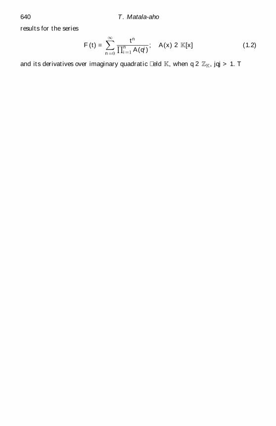
results for the series
F (t) =
1X
n = 0
tn
Qni = 1 A(qi)
; A(x) 2 K[x] (1.2)
and its derivatives over imaginary quadratic eld K, when q 2 ZK, jqj > 1. T�opfer[21] considered linear independence of the solutions and their derivatives in somespecial cases of (1.1). In the special case qtF (q2t) = ¡ F (qt) + F (t) attached tothe Rogers{Ramanujan continued fraction sharp irrationality measures have beenobtained by Bundschuh [4] and Shiokawa [17] in the imaginary quadratic eld caseand by Matala-aho [10] when K is an algebraic number eld.
On the other hand, there is much work considering the arithmetic nature of theq-hypergeometric series k © l(t) (see Stihl [19] and Katsudara [9]) and of the analyticsolutions F (t) of the rst degree q-functional equation
A(q; t)F (qt) = B(q; t)F (t) + C(q; t);
see [1,4{7,13,14,16,18,20{22].In the rst part we shall state and prove linear independence results. Theorem 3.3
is especially designed to study quantitative aspects of q-functions and it is written insuch a way that we do not need to multiply any denominators in the approximationformulae, all information is now included in the heights via the product formula(2.1).
Then we shall tackle equation (1.1) with N (q; t) = tsM(q; t) when the positiveinteger s and the degrees r0 = degt M (q; t), ri = degt Pi(q; t) in t of the coe¯ cientpolynomials satisfy the condition (4.2). The new phenomenon coming from the useof the functional equation method is that we do not need to know a priori anyexplicit forms for the solutions of equation (1.1). Only property of the solutionsneeded is a slight upper bound condition near zero, we shall use the condition(4.3). The methods using rational function approximations (Pad́e approximations)or Thue-Siegel’s lemma usually need explicit knowledge of the behaviour of theq-series expansions. The crucial thing in studying equation (1.1) is to use matrixformalism for the functional equation method, which enables us to achieve trans-parent estimations for the approximation polynomials (3.2) and for the remainderterm (3.3) and an easy determination of the determinant condition (3.4).
As a consequence of using the functional equation method, we are able to applytheorems 3.1 and 3.3 not only for the analytic solutions including the class ofq-hypergeometric series studied by Stihl [19] and partly for the class of functions(1.2) studied by B´ezivin [2] and recently by Amou et al . [1], but also for other|evennon-continuous|solutions of (1.1). Our main result, theorem 4.1, for the non-zerosolutions of equation (1.1) is that under the conditions (4.2){(4.4) at least two ofthe numbers
F (t); F (qt); : : : ; F (qm¡1t) (1.3)
are linearly independent over K (an algebraic number eld) having a linear inde-pendence measure depending on the degrees s, ri (i = 1; : : : ; m) and the dimensionof the vector space generated by the numbers (1.3).
The case m = 2 has interesting implications for the values of certain q-continuedfractions (see [10,12]).

Diophantine approximations 641
2. Notation
Let K be an algebraic number eld of degree µ over Q. If the nite place v of Klies over the prime p, we write vjp, for an in nite place v of K we write vj1. Wenormalize the absolute value kv of K so that
if vjp; then jpjv = p¡1;
if vj1; then jxjv = jxj;
where j ¢ j denotes the ordinary absolute value in Q. By using the normalized valu-ations
k ¬ kv = j¬ jµ v =µv ; µv = [Kv : Qv ];
the product formula has the form
Y
v
k ¬ kv = 1 8 ¬ 2 K ¤ : (2.1)
The Height H( ¬ ) of ¬ is de ned by the formula
H( ¬ ) =Y
v
k ¬ k ¤v; k¬ k ¤
v = maxf1; k ¬ kvg
and the height H( ¬ ) of vector ¬ = ( ¬ 1; : : : ; ¬ m) 2 Km is given by
H( ¬ ) =Y
v
k ¬ k¤v ; k ¬ k ¤
v = maxi= 1;:::;m
f1; k ¬ ikvg:
We shall also use the notation
Kv( ) =Y
w 6= v
maxi = 1;:::;d
k ikw;
Lv( ) = mini = 1;:::;d
maxj 6= i
k jkvKv( )
for any vector = ( 1; : : : ; d) 2 Kd and
K( ·B) =Y
v
maxi;j
kbi;jkv
for any matrix ·B = (bi;j). Here the quantity mini = 1;:::;d maxj 6= i k jkv gives a secondlargest number of kbjk, j = 1; : : : ; d, and the introduction of Lv( ) is essential inthe following argument. For any place v of K, q 2 K ¤ and kqkv 6= 1, we de ne thenumber
¶ = ¶ q =log H(q)
log kqkv
having the following properties ¶ 1=q = ¡ ¶ q, j¶ q j > 1. Also ¶ q 6 ¡ 1 for all jqjv < 1,and ¶ q = ¡ 1; if moreover jqjw > 1 for all w 6= v:
642 T. Matala-aho
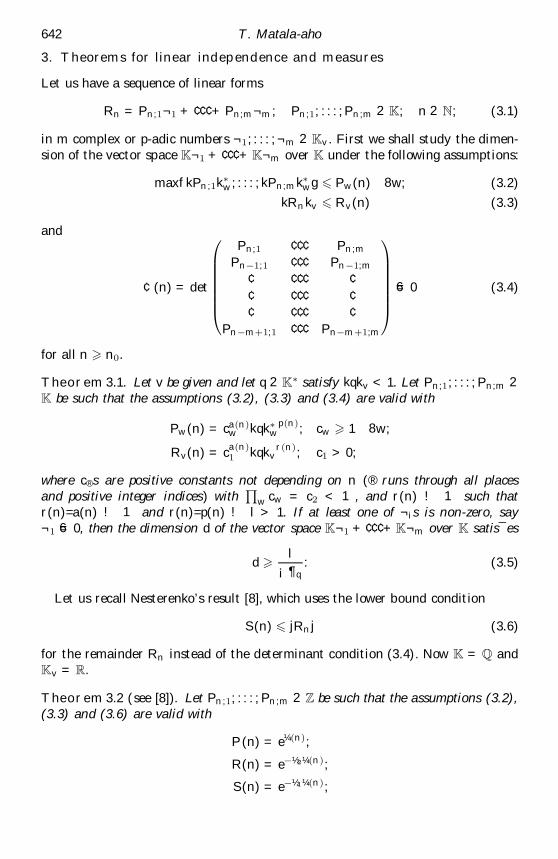
3. Theorems for linear independence and measures
Let us have a sequence of linear forms
Rn = Pn;1 ¬ 1 + ¢ ¢ ¢ + Pn;m ¬ m; Pn;1; : : : ; Pn;m 2 K; n 2 N; (3.1)
in m complex or p-adic numbers ¬ 1; : : : ; ¬ m 2 Kv . First we shall study the dimen-sion of the vector space K ¬ 1 + ¢ ¢ ¢ + K ¬ m over K under the following assumptions:
maxfkPn;1k ¤w; : : : ; kPn;mk¤
wg 6 Pw(n) 8w; (3.2)
kRnkv 6 Rv(n) (3.3)
and
¢ (n) = det
0
BBBBBB@
Pn;1 ¢ ¢ ¢ Pn;m
Pn¡1;1 ¢ ¢ ¢ Pn¡1;m
¢ ¢ ¢ ¢ ¢¢ ¢ ¢ ¢ ¢¢ ¢ ¢ ¢ ¢
Pn¡m+ 1;1 ¢ ¢ ¢ Pn¡m + 1;m
1
CCCCCCA6= 0 (3.4)
for all n > n0.
Theorem 3.1. Let v be given and let q 2 K ¤ satisfy kqkv < 1. Let Pn;1; : : : ; Pn;m 2K be such that the assumptions (3.2), (3.3) and (3.4) are valid with
Pw(n) = ca(n)w kqk ¤
wp(n)
; cw > 1 8w;
Rv(n) = ca(n)1 kqkv
r(n); c1 > 0;
where c ® s are positive constants not depending on n ( ® runs through all placesand positive integer indices) with
Qw cw = c2 < 1, and r(n) ! 1 such that
r(n)=a(n) ! 1 and r(n)=p(n) ! l > 1. If at least one of ¬ is is non-zero, say¬ 1 6= 0, then the dimension d of the vector space K ¬ 1 + ¢ ¢ ¢ + K ¬ m over K satis¯es
d > l
¡ ¶ q: (3.5)
Let us recall Nesterenko’s result [8], which uses the lower bound condition
S(n) 6 jRnj (3.6)
for the remainder Rn instead of the determinant condition (3.4). Now K = Q andKv = R.
Theorem 3.2 (see [8]). Let Pn;1; : : : ; Pn;m 2 Z be such that the assumptions (3.2),(3.3) and (3.6) are valid with
P (n) = e¼ (n);
R(n) = e¡ ½ 2 ¼ (n);
S(n) = e¡ ½ 1 ¼ (n);
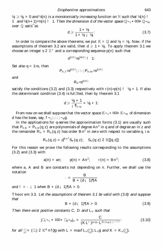
Diophantine approximations 643
½ 1 > ½ 2 > 0 and ¼ (n) is a monotonical ly increasing function on N such that ¼ (n) !1 and ¼ (n+1)=¼ (n) ! 1. Then the dimension d of the vector space Q ¬ 1+¢ ¢ ¢+Q ¬ m
over Q satis¯es
d > 1 + ½ 1
1 + ½ 1 ¡ ½ 2: (3.7)
In order to compare the above theorems, we put K = Q and ½ 1 = ½ 2. Now, if theassumptions of theorem 3.2 are valid, then d > 1 + ½ 2. To apply theorem 3.1 wechoose an integer s 2 Z + and a corresponding sequence p(n) such that
sp(n)=e ¼ (n) ! 1:
Set also q = 1=s, thenPn;1=sp(n); : : : ; Pn;m=sp(n)
andRn=sp(n)
satisfy the conditions (3.2) and (3.3) respectively with r(n)=p(n) ! ½ 2 + 1. If alsothe determinant condition (3.4) is ful lled, then by theorem 3.1
d > ½ 2 + 1
¡ ¶ 1=s= ½ 2 + 1:
From now on we shall suppose that the vector space K ¬ 1+¢ ¢ ¢+K ¬ m of dimensiond has the base, say, f ¬ 1; : : : ; ¬ dg.
In the applications for q-series the approximation forms (3.1) are usually suchthat Pn;k = Pn;k(q; z) are polynomials of degree An2 in q and of degree an in z andthe remainder Rn = Rn(q; z) has order Bn2 in zero with respect to variable q, i.e.
Rn(q; z) = qBn2
Sn(q; z); Sn(q; z) 2 K[[q; z]]:
For this reason we prove the following results corresponding to the assumptions(3.2) and (3.3) with
a(n) = an; p(n) = An2; r(n) = Bn2; (3.8)
where a, A and B are constants not depending on n. Further, we shall use thenotation
· =B
B + (d ¡ 1)¶ A
and ! = · ¡ 1 when B + (d ¡ 1)¶ A > 0.
Theorem 3.3. Let the assumptions of theorem 3.1 be valid with (3.8) and supposethat
B + (d ¡ 1)¶ A > 0: (3.9)
Then there exist positive constants C, D and L0 such that
j 1 ¬ 1 + ¢ ¢ ¢ + d ¬ djv >C
(KL!) µ =µ v LD(log L) ¡ 1=2 : (3.10)
for all = ( i) 2 Kd n f0g with L = maxfLv( ); L0g and K = Kv( ).
644 T. Matala-aho
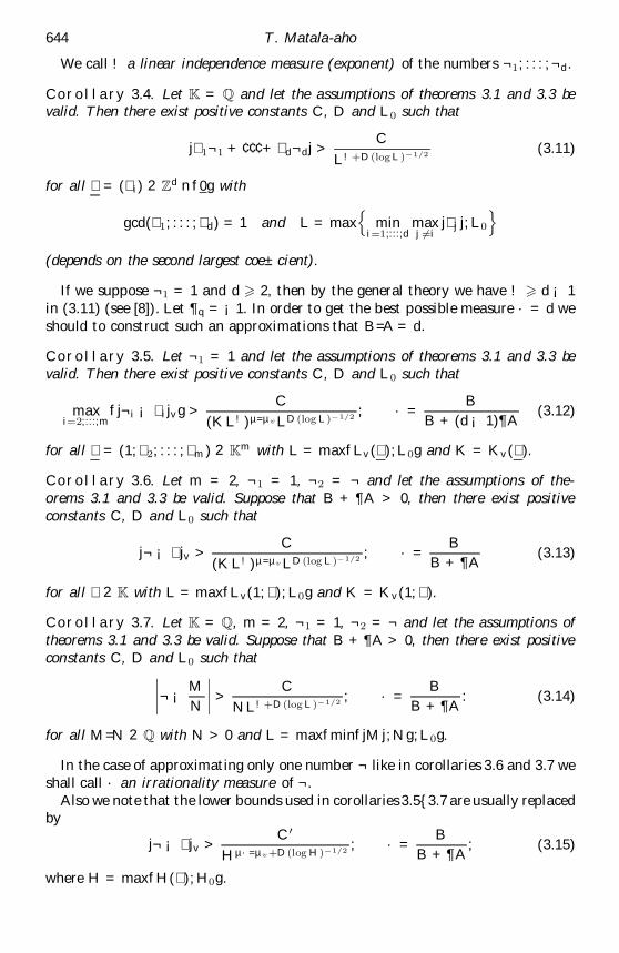
We call ! a linear independence measure (exponent) of the numbers ¬ 1; : : : ; ¬ d.
Corollary 3.4. Let K = Q and let the assumptions of theorems 3.1 and 3.3 bevalid. Then there exist positive constants C, D and L0 such that
j 1 ¬ 1 + ¢ ¢ ¢ + d ¬ dj >C
L! + D(log L) ¡ 1=2 (3.11)
for all = ( i) 2 Zd n f0g with
gcd( 1; : : : ; d) = 1 and L = maxn
mini = 1;:::;d
maxj 6= i
j j j; L0
o
(depends on the second largest coe± cient).
If we suppose ¬ 1 = 1 and d > 2, then by the general theory we have ! > d ¡ 1in (3.11) (see [8]). Let ¶ q = ¡ 1. In order to get the best possible measure · = d weshould to construct such an approximations that B=A = d.
Corollary 3.5. Let ¬ 1 = 1 and let the assumptions of theorems 3.1 and 3.3 bevalid. Then there exist positive constants C, D and L0 such that
maxi= 2;:::;m
fj¬ i ¡ ijvg >C
(KL!) µ =µ v LD(log L) ¡ 1=2 ; · =B
B + (d ¡ 1)¶ A(3.12)
for all = (1; 2; : : : ; m) 2 Km with L = maxfLv( ); L0g and K = Kv( ).
Corollary 3.6. Let m = 2, ¬ 1 = 1, ¬ 2 = ¬ and let the assumptions of the-orems 3.1 and 3.3 be valid. Suppose that B + ¶ A > 0, then there exist positiveconstants C, D and L0 such that
j ¬ ¡ jv >C
(KL!) µ =µ v LD(log L)¡ 1=2 ; · =B
B + ¶ A(3.13)
for all 2 K with L = maxfLv(1; ); L0g and K = Kv(1; ).
Corollary 3.7. Let K = Q, m = 2, ¬ 1 = 1, ¬ 2 = ¬ and let the assumptions oftheorems 3.1 and 3.3 be valid. Suppose that B + ¶ A > 0, then there exist positiveconstants C, D and L0 such that
¯̄¯̄ ¬ ¡ M
N
¯̄¯̄ >
C
NL! + D(log L) ¡ 1=2; · =
B
B + ¶ A: (3.14)
for all M=N 2 Q with N > 0 and L = maxfminfjM j; Ng; L0g.
In the case of approximating only one number ¬ like in corollaries 3.6 and 3.7 weshall call · an irrationality measure of ¬ .
Also we note that the lower bounds used in corollaries 3.5{3.7 are usually replacedby
j¬ ¡ jv >C 0
H µ · =µ v + D(log H) ¡ 1=2 ; · =B
B + ¶ A; (3.15)
where H = maxfH( ); H0g.
Diophantine approximations 645
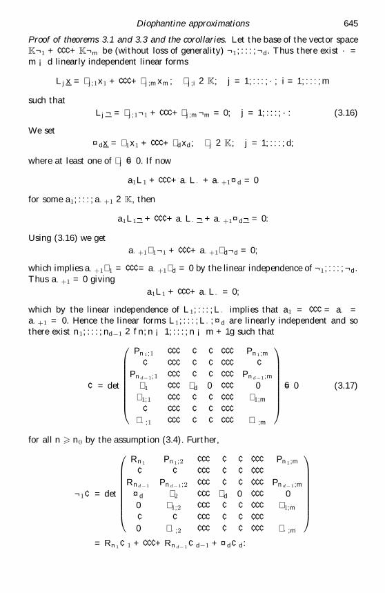
Proof of theorems 3.1 and 3.3 and the corollaries. Let the base of the vector spaceK ¬ 1 + ¢ ¢ ¢ + K ¬ m be (without loss of generality) ¬ 1; : : : ; ¬ d. Thus there exist · =m ¡ d linearly independent linear forms
Ljx = j;1x1 + ¢ ¢ ¢ + j;mxm; j;i 2 K; j = 1; : : : ; · ; i = 1; : : : ; m
such that
Lj ¬ = j;1 ¬ 1 + ¢ ¢ ¢ + j;m ¬ m = 0; j = 1; : : : ; · : (3.16)
We set
¤ dx = 1x1 + ¢ ¢ ¢ + dxd; j 2 K; j = 1; : : : ; d;
where at least one of j 6= 0. If now
a1L1 + ¢ ¢ ¢ + a · L · + a · + 1 ¤ d = 0
for some a1; : : : ; a · + 1 2 K, then
a1L1 ¬ + ¢ ¢ ¢ + a · L · ¬ + a · + 1 ¤ d ¬ = 0:
Using (3.16) we get
a · + 1 1 ¬ 1 + ¢ ¢ ¢ + a · + 1 d ¬ d = 0;
which implies a · + 1 1 = ¢ ¢ ¢ = a· + 1 d = 0 by the linear independence of ¬ 1; : : : ; ¬ d.Thus a · + 1 = 0 giving
a1L1 + ¢ ¢ ¢ + a · L · = 0;
which by the linear independence of L1; : : : ; L · implies that a1 = ¢ ¢ ¢ = a · =a · + 1 = 0. Hence the linear forms L1; : : : ; L · ; ¤ d are linearly independent and sothere exist n1; : : : ; nd¡1 2 fn; n ¡ 1; : : : ; n ¡ m + 1g such that
¢ = det
0
BBBBBBBB@
Pn1;1 ¢ ¢ ¢ ¢ ¢ ¢ ¢ ¢ Pn1;m
¢ ¢ ¢ ¢ ¢ ¢ ¢ ¢ ¢ ¢Pnd ¡ 1;1 ¢ ¢ ¢ ¢ ¢ ¢ ¢ ¢ Pnd ¡ 1;m
1 ¢ ¢ ¢ d 0 ¢ ¢ ¢ 0
1;1 ¢ ¢ ¢ ¢ ¢ ¢ ¢ ¢ 1;m
¢ ¢ ¢ ¢ ¢ ¢ ¢ ¢ ¢ · ;1 ¢ ¢ ¢ ¢ ¢ ¢ ¢ ¢ · ;m
1
CCCCCCCCA
6= 0 (3.17)
for all n > n0 by the assumption (3.4). Further,
¬ 1 ¢ = det
0
BBBBBBBB@
Rn1 Pn1;2 ¢ ¢ ¢ ¢ ¢ ¢ ¢ ¢ Pn1;m
¢ ¢ ¢ ¢ ¢ ¢ ¢ ¢ ¢ ¢Rnd ¡ 1 Pnd ¡ 1;2 ¢ ¢ ¢ ¢ ¢ ¢ ¢ ¢ Pnd ¡ 1;m
¤ d 2 ¢ ¢ ¢ d 0 ¢ ¢ ¢ 0
0 1;2 ¢ ¢ ¢ ¢ ¢ ¢ ¢ ¢ 1;m
¢ ¢ ¢ ¢ ¢ ¢ ¢ ¢ ¢ ¢0 · ;2 ¢ ¢ ¢ ¢ ¢ ¢ ¢ ¢ · ;m
1
CCCCCCCCA
= Rn1 ¢ 1 + ¢ ¢ ¢ + Rnd ¡ 1 ¢ d¡1 + ¤ d ¢ d:
646 T. Matala-aho
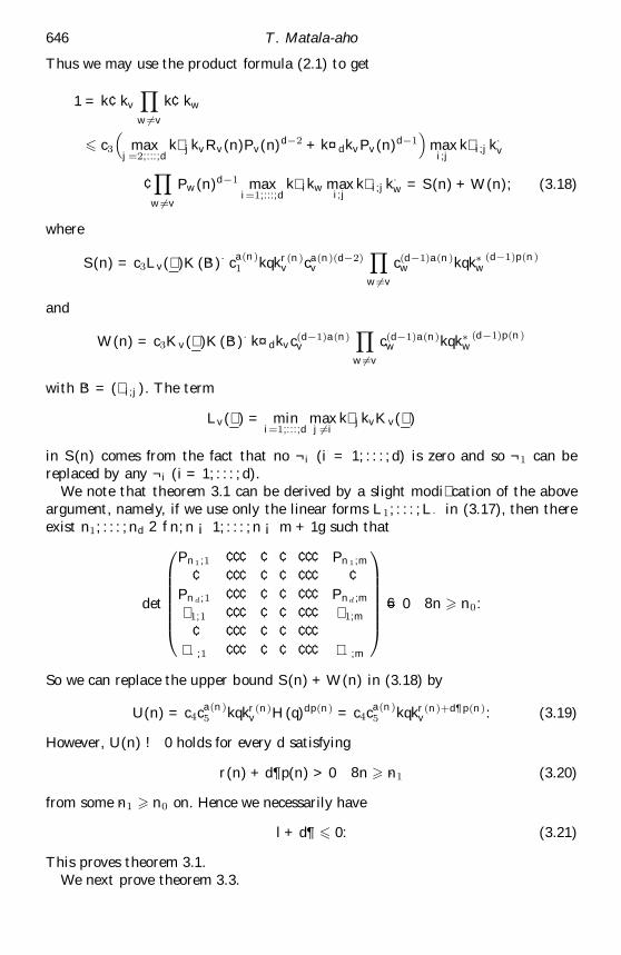
Thus we may use the product formula (2.1) to get
1 = k ¢ kv
Y
w 6= v
k¢ kw
6 c3
³max
j = 2;:::;dk jkvRv(n)Pv(n)d¡2 + k ¤ dkvPv(n)d¡1
´max
i;jk i;jk ·
v
¢Y
w 6= v
Pw(n)d¡1 maxi = 1;:::;d
k ikw maxi;j
k i;jk ·w = S(n) + W (n); (3.18)
where
S(n) = c3Lv( )K( ·B) · ca(n)1 kqkr(n)
v ca(n)(d¡2)v
Y
w 6= v
c(d¡1)a(n)w kqk¤
w(d¡1)p(n)
and
W (n) = c3Kv( )K( ·B) · k ¤ dkvc(d¡1)a(n)v
Y
w 6= v
c(d¡1)a(n)w kqk ¤
w(d¡1)p(n)
with ·B = ( i;j). The term
Lv( ) = mini = 1;:::;d
maxj 6= i
k jkvKv( )
in S(n) comes from the fact that no ¬ i (i = 1; : : : ; d) is zero and so ¬ 1 can bereplaced by any ¬ i (i = 1; : : : ; d).
We note that theorem 3.1 can be derived by a slight modi cation of the aboveargument, namely, if we use only the linear forms L1; : : : ; L · in (3.17), then thereexist n1; : : : ; nd 2 fn; n ¡ 1; : : : ; n ¡ m + 1g such that
det
0
BBBBBB@
Pn1 ;1 ¢ ¢ ¢ ¢ ¢ ¢ ¢ ¢ Pn1;m
¢ ¢ ¢ ¢ ¢ ¢ ¢ ¢ ¢ ¢Pnd;1 ¢ ¢ ¢ ¢ ¢ ¢ ¢ ¢ Pnd ;m
1;1 ¢ ¢ ¢ ¢ ¢ ¢ ¢ ¢ 1;m
¢ ¢ ¢ ¢ ¢ ¢ ¢ ¢ ¢ · ;1 ¢ ¢ ¢ ¢ ¢ ¢ ¢ ¢ · ;m
1
CCCCCCA6= 0 8n > n0:
So we can replace the upper bound S(n) + W (n) in (3.18) by
U (n) = c4ca(n)5 kqkr(n)
v H(q)dp(n) = c4ca(n)5 kqkr(n)+ d¶ p(n)
v : (3.19)
However, U (n) ! 0 holds for every d satisfying
r(n) + d¶ p(n) > 0 8n > ·n1 (3.20)
from some ·n1 > n0 on. Hence we necessarily have
l + d¶ 6 0: (3.21)
This proves theorem 3.1.We next prove theorem 3.3.
Diophantine approximations 647
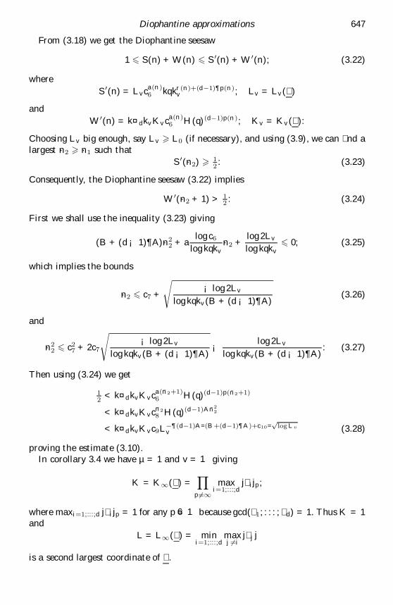
From (3.18) we get the Diophantine seesaw
1 6 S(n) + W (n) 6 S 0(n) + W 0(n); (3.22)
where
S 0(n) = Lvca(n)6 kqkr(n)+ (d¡1) ¶ p(n)
v ; Lv = Lv( )
and
W 0(n) = k ¤ dkvKvca(n)6 H(q)(d¡1)p(n); Kv = Kv( ):
Choosing Lv big enough, say Lv > L0 (if necessary), and using (3.9), we can nd alargest ·n2 > ·n1 such that
S 0(·n2) > 12: (3.23)
Consequently, the Diophantine seesaw (3.22) implies
W 0(·n2 + 1) > 12 : (3.24)
First we shall use the inequality (3.23) giving
(B + (d ¡ 1)¶ A)·n22 + a
log c6
log kqkv·n2 +
log 2Lv
log kqkv6 0; (3.25)
which implies the bounds
·n2 6 c7 +
s¡ log 2Lv
log kqkv(B + (d ¡ 1)¶ A)(3.26)
and
·n22 6 c2
7 + 2c7
s¡ log 2Lv
log kqkv(B + (d ¡ 1)¶ A)¡ log 2Lv
log kqkv(B + (d ¡ 1)¶ A): (3.27)
Then using (3.24) we get
12
< k ¤ dkvKvca(·n2 + 1)6 H(q)(d¡1)p(·n2 + 1)
< k ¤ dkvKvc·n2
8 H(q)(d¡1)A·n22
< k ¤ dkvKvc9L¡ ¶ (d¡1)A=(B + (d¡1) ¶ A)+ c10=p
log Lvv (3.28)
proving the estimate (3.10).In corollary 3.4 we have µ = 1 and v = 1 giving
K = K 1 ( ) =Y
p6= 1max
i = 1;:::;dj ijp;
where maxi = 1;:::;d j ijp = 1 for any p 6= 1 because gcd( 1; : : : ; d) = 1. Thus K = 1and
L = L 1 ( ) = mini = 1;:::;d
maxj 6= i
j j j
is a second largest coordinate of .

648 T. Matala-aho
In corollary 3.5 the dimension d of the vector space K ¬ 1 + ¢ ¢ ¢ + K ¬ m is at least2 having a base f1; : : : ; ¬ j ; : : : g. From (3.10) we get
j¬ j ¡ j jv >C
(K 0L0!) µ =µ v L0D(log L 0 ) ¡ 1=2; · =
B
B + ¶ A(3.29)
for any j 2 K with 0 = ( ¡ j ; 0; : : : ; 0; 1; 0; : : : ) 2 Km, L0 = maxfLv( 0); L00g and
K 0 = Kv( 0). This immediately gives (3.12).Corollary 3.6 follows directly from corollary 3.5.In corollary 3.7
K = K 1 =Y
p6= 1max
½1;
¯̄¯̄M
N
¯̄¯̄p
¾= N
and
L = L 1 = min
½1;
¯̄¯̄M
N
¯̄¯̄¾
N = minfN; jM jg
giving (3.14).
4. q-series
Let F (t) be a non-zero solution of the q-functional equation
tsMF (qmt) = P0;1F (qm¡1t) + P0;2F (qm¡2t) + ¢ ¢ ¢ + P0;mF (t) (4.1)
of lowest order m, where m > 2, s > 1 and M = M (q; t), P0;i = P0;i(q; t) 2 K[q; t]are of degree
r = degt M; ri = degt P0;i:
In the following we set
A = maxj = 2;:::;m
½r1;
(j ¡ 1)(s + r) + rj
2j
¾; B = 1
2s
and we supposeB > A: (4.2)
Theorem 4.1. Let v be a place of K and let q; t 2 K ¤ satisfy B + ¶ A > 0, jqjv < 1,M (q; qkt) 6= 0 and P0;m(q; qkt) 6= 0 for all k 2 N. Let F (t) be a solution of thefunctional equation (4.1) such that
jF (qnt)jv < cn11 8n 2 N (4.3)
for some positive constant c11 and the numbers
F (t); F (qt); : : : ; F (qm¡1t) (4.4)
are not all zero, then
d = dimKfKF (t) + KF (qt) + ¢ ¢ ¢ + KF (qm¡1t)g > 2:
If d = 2, then any two of the numbers (4.4) being linearly independent over K havea linear independence measure ! = · ¡ 1, where · = B=(B + ¶ A).
Diophantine approximations 649
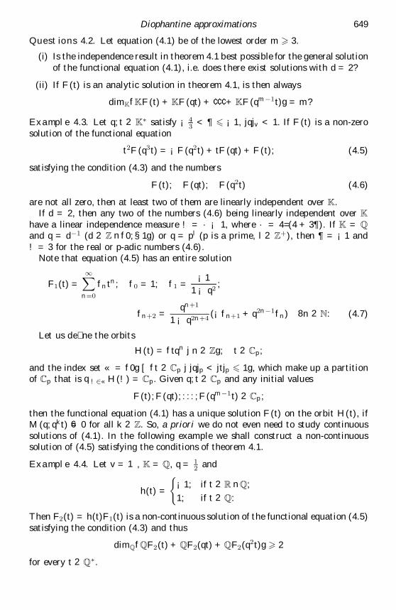
Questions 4.2. Let equation (4.1) be of the lowest order m > 3.
(i) Is the independence result in theorem 4.1 best possible for the general solutionof the functional equation (4.1), i.e. does there exist solutions with d = 2?
(ii) If F (t) is an analytic solution in theorem 4.1, is then always
dimKfKF (t) + KF (qt) + ¢ ¢ ¢ + KF (qm¡1t)g = m?
Example 4.3. Let q; t 2 K ¤ satisfy ¡ 43
< ¶ 6 ¡ 1, jqjv < 1. If F (t) is a non-zerosolution of the functional equation
t2F (q3t) = ¡ F (q2t) + tF (qt) + F (t); (4.5)
satisfying the condition (4.3) and the numbers
F (t); F (qt); F (q2t) (4.6)
are not all zero, then at least two of them are linearly independent over K.If d = 2, then any two of the numbers (4.6) being linearly independent over K
have a linear independence measure ! = · ¡ 1, where · = 4=(4 + 3 ¶ ). If K = Qand q = d¡1 (d 2 Z n f0; §1g) or q = pl (p is a prime, l 2 Z+ ), then ¶ = ¡ 1 and! = 3 for the real or p-adic numbers (4.6).
Note that equation (4.5) has an entire solution
F1(t) =
1X
n = 0
fntn; f0 = 1; f1 =¡ 1
1 ¡ q2;
fn + 2 =qn + 1
1 ¡ q2n + 4( ¡ fn+ 1 + q2n¡1fn) 8n 2 N: (4.7)
Let us de ne the orbits
H(t) = ftqn j n 2 Zg; t 2 Cp;
and the index set « = f0g [ ft 2 Cp j jqjp < jtjp 6 1g, which make up a partitionof Cp that is q! 2 « H(!) = Cp. Given q; t 2 Cp and any initial values
F (t); F (qt); : : : ; F (qm¡1t) 2 Cp;
then the functional equation (4.1) has a unique solution F (t) on the orbit H(t), ifM (q; qkt) 6= 0 for all k 2 Z. So, a priori we do not even need to study continuoussolutions of (4.1). In the following example we shall construct a non-continuoussolution of (4.5) satisfying the conditions of theorem 4.1.
Example 4.4. Let v = 1, K = Q, q = 12 and
h(t) =
(¡ 1; if t 2 R n Q;
1; if t 2 Q:
Then F2(t) = h(t)F1(t) is a non-continuous solution of the functional equation (4.5)satisfying the condition (4.3) and thus
dimQfQF2(t) + QF2(qt) + QF2(q2t)g > 2
for every t 2 Q ¤ .
650 T. Matala-aho
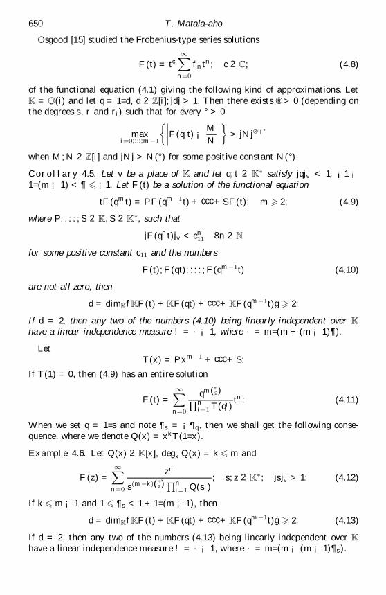
Osgood [15] studied the Frobenius-type series solutions
F (t) = tc1X
n = 0
fntn; c 2 C; (4.8)
of the functional equation (4.1) giving the following kind of approximations. LetK = Q(i) and let q = 1=d, d 2 Z[i]; jdj > 1. Then there exists ® > 0 (depending onthe degrees s, r and ri) such that for every ° > 0
maxi = 0;:::;m¡1
½¯̄¯̄F (qit) ¡ M
N
¯̄¯̄¾
> jN j® + °
when M; N 2 Z[i] and jN j > N ( ° ) for some positive constant N( ° ).
Corollary 4.5. Let v be a place of K and let q; t 2 K ¤ satisfy jqjv < 1, ¡ 1 ¡1=(m ¡ 1) < ¶ 6 ¡ 1. Let F (t) be a solution of the functional equation
tF (qmt) = PF (qm¡1t) + ¢ ¢ ¢ + SF (t); m > 2; (4.9)
where P; : : : ; S 2 K; S 2 K ¤ , such that
jF (qnt)jv < cn11 8n 2 N
for some positive constant c11 and the numbers
F (t); F (qt); : : : ; F (qm¡1t) (4.10)
are not all zero, then
d = dimKfKF (t) + KF (qt) + ¢ ¢ ¢ + KF (qm¡1t)g > 2:
If d = 2, then any two of the numbers (4.10) being linearly independent over Khave a linear independence measure ! = · ¡ 1, where · = m=(m + (m ¡ 1)¶ ).
LetT (x) = Pxm¡1 + ¢ ¢ ¢ + S:
If T (1) = 0, then (4.9) has an entire solution
F (t) =
1X
n= 0
qm(n2)
Qni = 1 T (qi)
tn: (4.11)
When we set q = 1=s and note ¶ s = ¡ ¶ q, then we shall get the following conse-quence, where we denote Q(x) = xkT (1=x).
Example 4.6. Let Q(x) 2 K[x], degx Q(x) = k 6 m and
F (z) =
1X
n = 0
zn
s(m¡k)(n2) Qn
i = 1 Q(si); s; z 2 K ¤ ; jsjv > 1: (4.12)
If k 6 m ¡ 1 and 1 6 ¶ s < 1 + 1=(m ¡ 1), then
d = dimKfKF (t) + KF (qt) + ¢ ¢ ¢ + KF (qm¡1t)g > 2: (4.13)
If d = 2, then any two of the numbers (4.13) being linearly independent over Khave a linear independence measure ! = · ¡ 1, where · = m=(m ¡ (m ¡ 1) ¶ s).

Diophantine approximations 651
The results of B́ezivin [2] imply qualitative linear independence results over theimaginary quadratic eld K for the series (4.12) and its derivatives, if s; t 2 K ¤ ; s 2ZK; jsj > 1, where ZK denotes the ring of integers in K.
Let
Bq(z) =
1X
n = 0
zn
(q)n(q)n
be the q-analogue of the Bessel function. Matala-aho [11] proved an irrationalitymeasure · = 7=(7 ¡ 4¶ s) over K for Bs(s) with s 2 K, jsjv > 1 and 1 6 ¶ s < 7=4.
Duverney [7] used Thue-Siegel lemma to construct approximations for the solu-tions in the form (4.12) of the equation
zsf (z) = P (z)f (dz) + Q(z): (4.14)
In Amov et al . [1] Thue-Siegel’s method is developed in a signi cant manner toget irrationality measures for the functions (4.12) over algebraic number elds K.
Based on the Pad́e approximations of q-hypergeometric series Stihl [19] hasproved linear independence results over Q in the archimedean case with measuresfor a class of q-hypergeometric series which interlace partly with our analytic solu-tions of the functional equation (4.9).
In the following example a comparison is made in certain common cases betweenthe results coming from our corollary 4.5, Theorem 2 of Amou et al . [1] and Satz1-2 of Stihl [19].
Example 4.7. Now we shall restrict to the archimedean case in K = Q. The q-hypergeometric series
F (t) =
1X
n = 0
qm(n2)
(q)n(a1)n : : : (al)ntn; m > 2; l 6 m ¡ 2; (4.15)
satis es the functional equation
tF (qmt) = dl + 1F (ql + 1t) + dlF (qlt) + ¢ ¢ ¢ + d0F (t); (4.16)
where
dl + 1xl+ 1 + dlxl + ¢ ¢ ¢ + d0 = (1 ¡ qx)(1 ¡ a1x) : : : (1 ¡ alx): (4.17)
If di = di(a1; : : : ; al) 2 Q (i = 1; : : : ; l + 1), then corollary 4.5 gives the linearindependence over Q of at least two of the numbers
F (t); F (qt); : : : ; F (qm¡1t) (4.18)
for all q = r=s; t 2 Q ¤ satisfying s > jrjm. If d = 2, then any two of the numbers(4.18) being linearly independent over K have a linear independence measure ! =· ¡ 1, where
· = mlog(r=s)
log(rm=s):
From Amou et al . [1] it follows that the numbers (4.18) are irrational for allq = r=s, t 2 Q ¤ , satisfying s > jrj¡ 1 , where ¡ 1 = ¡ 1(m) (is a computable positive
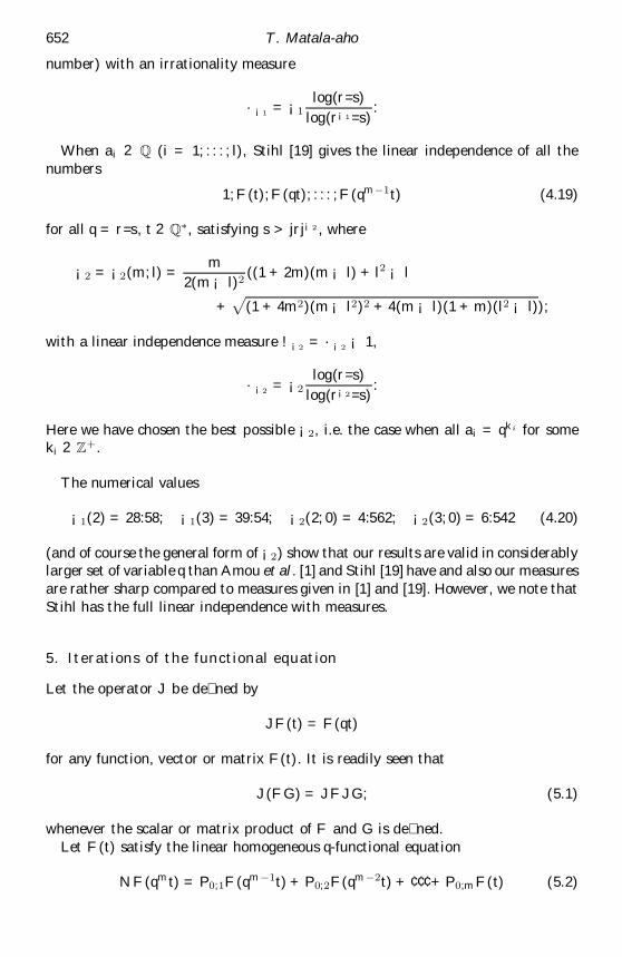
652 T. Matala-aho
number) with an irrationality measure
· ¡ 1 = ¡ 1log(r=s)
log(r ¡ 1 =s):
When ai 2 Q (i = 1; : : : ; l), Stihl [19] gives the linear independence of all thenumbers
1; F (t); F (qt); : : : ; F (qm¡1t) (4.19)
for all q = r=s, t 2 Q ¤ , satisfying s > jrj¡ 2 , where
¡ 2 = ¡ 2(m; l) =m
2(m ¡ l)2((1 + 2m)(m ¡ l) + l2 ¡ l
+p
(1 + 4m2)(m ¡ l2)2 + 4(m ¡ l)(1 + m)(l2 ¡ l));
with a linear independence measure ! ¡ 2 = · ¡ 2 ¡ 1,
· ¡ 2 = ¡ 2log(r=s)
log(r ¡ 2 =s):
Here we have chosen the best possible ¡ 2, i.e. the case when all ai = qki for someki 2 Z + .
The numerical values
¡ 1(2) = 28:58; ¡ 1(3) = 39:54; ¡ 2(2; 0) = 4:562; ¡ 2(3; 0) = 6:542 (4.20)
(and of course the general form of ¡ 2) show that our results are valid in considerablylarger set of variable q than Amou et al . [1] and Stihl [19] have and also our measuresare rather sharp compared to measures given in [1] and [19]. However, we note thatStihl has the full linear independence with measures.
5. Iterations of the functional equation
Let the operator J be de ned by
JF (t) = F (qt)
for any function, vector or matrix F (t). It is readily seen that
J(F G) = JF JG; (5.1)
whenever the scalar or matrix product of F and G is de ned.Let F (t) satisfy the linear homogeneous q-functional equation
NF (qmt) = P0;1F (qm¡1t) + P0;2F (qm¡2t) + ¢ ¢ ¢ + P0;mF (t) (5.2)
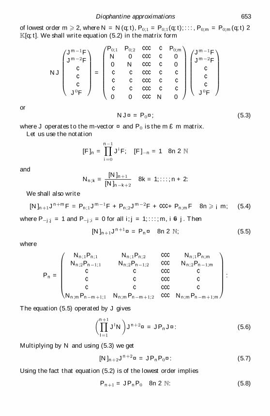
Diophantine approximations 653
of lowest order m > 2, where N = N (q; t), P0;1 = P0;1(q; t); : : : , P0;m = P0;m(q; t) 2K[q; t]. We shall write equation (5.2) in the matrix form
NJ
0
BBBBBB@
Jm¡1F
Jm¡2F
¢¢¢
J0F
1
CCCCCCA=
0
BBBBBBBB@
P0;1 P0;2 ¢ ¢ ¢ ¢ P0;m
N 0 ¢ ¢ ¢ ¢ 0
0 N ¢ ¢ ¢ ¢ 0
¢ ¢ ¢ ¢ ¢ ¢ ¢¢ ¢ ¢ ¢ ¢ ¢ ¢¢ ¢ ¢ ¢ ¢ ¢ ¢0 0 ¢ ¢ ¢ N 0
1
CCCCCCCCA
0
BBBBBB@
Jm¡1F
Jm¡2F
¢¢¢
J0F
1
CCCCCCA
orNJ ¤ = P0 ¤ ; (5.3)
where J operates to the m-vector ¤ and P0 is the m £ m matrix.Let us use the notation
[F ]n =
n¡1Y
i = 0
J iF; [F ]¡n = 1 8n 2 N
and
Nn;k =[N ]n+ 1
[N ]n¡k + 28k = 1; : : : ; n + 2:
We shall also write
[N ]n + 1Jn+ mF = Pn;1Jm¡1F + Pn;2Jm¡2F + ¢ ¢ ¢ + Pn;mF 8n > ¡ m; (5.4)
where P¡j;j = 1 and P¡j;i = 0 for all i; j = 1; : : : ; m, i 6= j. Then
[N ]n+ 1Jn + 1 ¤ = Pn ¤ 8n 2 N; (5.5)
where
Pn =
0
BBBBBB@
Nn;1Pn;1 Nn;1Pn;2 ¢ ¢ ¢ Nn;1Pn;m
Nn;2Pn¡1;1 Nn;2Pn¡1;2 ¢ ¢ ¢ Nn;2Pn¡1;m
¢ ¢ ¢ ¢ ¢ ¢¢ ¢ ¢ ¢ ¢ ¢¢ ¢ ¢ ¢ ¢ ¢
Nn;mPn¡m + 1;1 Nn;mPn¡m+ 1;2 ¢ ¢ ¢ Nn;mPn¡m+ 1;m
1
CCCCCCA:
The equation (5.5) operated by J gives
µn + 1Y
l = 1
J lN
¶Jn+ 2 ¤ = JPnJ ¤ : (5.6)
Multiplying by N and using (5.3) we get
[N ]n+ 2Jn + 2 ¤ = JPnP0 ¤ : (5.7)
Using the fact that equation (5.2) is of the lowest order implies
Pn + 1 = JPnP0 8n 2 N: (5.8)
654 T. Matala-aho
On the other hand, equation (5.3) operated by Jn + 1 implies
Jn + 1NJn+ 2 ¤ = Jn+ 1P0Jn+ 1 ¤ : (5.9)
Multiplication of (5.9) byQn
l= 0 J lN and the use of (5.5) give
[N ]n + 2Jn+ 2 ¤ = Jn+ 1P0Pn ¤ : (5.10)
Hence by (5.5) and (5.10) we get
Pn+ 1 = Jn+ 1P0Pn 8n 2 N: (5.11)
Equations (5.8) and (5.11) may be considered the fundamental recurrence forms forthe functional equation (5.2).
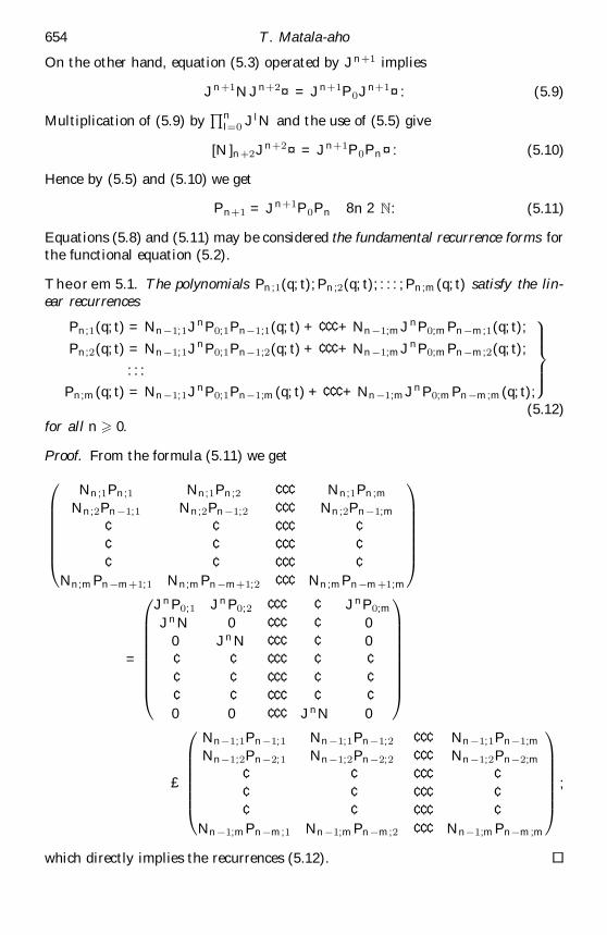
Theorem 5.1. The polynomials Pn;1(q; t); Pn;2(q; t); : : : ; Pn;m(q; t) satisfy the lin-ear recurrences
Pn;1(q; t) = Nn¡1;1JnP0;1Pn¡1;1(q; t) + ¢ ¢ ¢ + Nn¡1;mJ nP0;mPn¡m;1(q; t);
Pn;2(q; t) = Nn¡1;1JnP0;1Pn¡1;2(q; t) + ¢ ¢ ¢ + Nn¡1;mJ nP0;mPn¡m;2(q; t);
: : :
Pn;m(q; t) = Nn¡1;1JnP0;1Pn¡1;m(q; t) + ¢ ¢ ¢ + Nn¡1;mJnP0;mPn¡m;m(q; t);
9>>>=
>>>;
(5.12)for all n > 0.
Proof. From the formula (5.11) we get
0
BBBBBB@
Nn;1Pn;1 Nn;1Pn;2 ¢ ¢ ¢ Nn;1Pn;m
Nn;2Pn¡1;1 Nn;2Pn¡1;2 ¢ ¢ ¢ Nn;2Pn¡1;m
¢ ¢ ¢ ¢ ¢ ¢¢ ¢ ¢ ¢ ¢ ¢¢ ¢ ¢ ¢ ¢ ¢
Nn;mPn¡m+ 1;1 Nn;mPn¡m+ 1;2 ¢ ¢ ¢ Nn;mPn¡m + 1;m
1
CCCCCCA
=
0
BBBBBBBB@
JnP0;1 JnP0;2 ¢ ¢ ¢ ¢ JnP0;m
JnN 0 ¢ ¢ ¢ ¢ 0
0 JnN ¢ ¢ ¢ ¢ 0¢ ¢ ¢ ¢ ¢ ¢ ¢¢ ¢ ¢ ¢ ¢ ¢ ¢¢ ¢ ¢ ¢ ¢ ¢ ¢0 0 ¢ ¢ ¢ JnN 0
1
CCCCCCCCA
£
0
BBBBBB@
Nn¡1;1Pn¡1;1 Nn¡1;1Pn¡1;2 ¢ ¢ ¢ Nn¡1;1Pn¡1;m
Nn¡1;2Pn¡2;1 Nn¡1;2Pn¡2;2 ¢ ¢ ¢ Nn¡1;2Pn¡2;m
¢ ¢ ¢ ¢ ¢ ¢¢ ¢ ¢ ¢ ¢ ¢¢ ¢ ¢ ¢ ¢ ¢
Nn¡1;mPn¡m;1 Nn¡1;mPn¡m;2 ¢ ¢ ¢ Nn¡1;mPn¡m;m
1
CCCCCCA;
which directly implies the recurrences (5.12).
Diophantine approximations 655
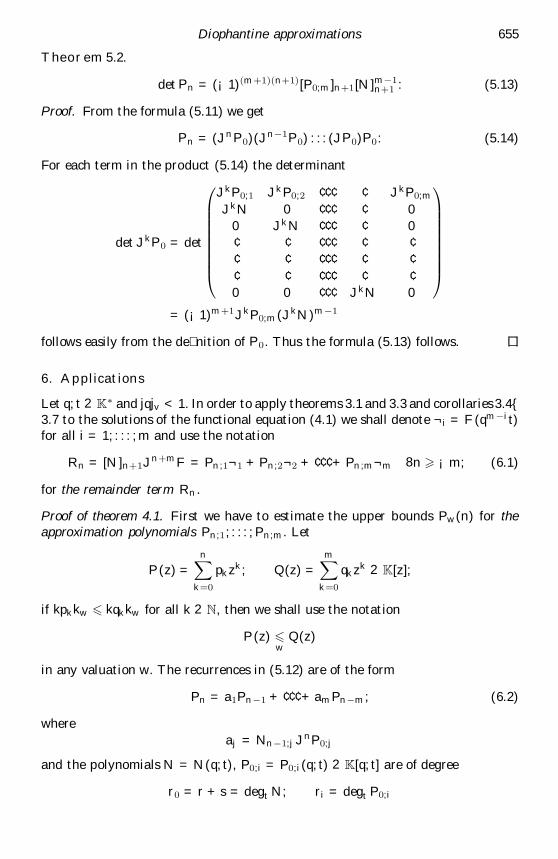
Theorem 5.2.
det Pn = ( ¡ 1)(m + 1)(n+ 1)[P0;m]n + 1[N ]m¡1n+ 1 : (5.13)
Proof. From the formula (5.11) we get
Pn = (JnP0)(Jn¡1P0) : : : (JP0)P0: (5.14)
For each term in the product (5.14) the determinant
det JkP0 = det
0
BBBBBBBB@
JkP0;1 JkP0;2 ¢ ¢ ¢ ¢ JkP0;m
JkN 0 ¢ ¢ ¢ ¢ 0
0 JkN ¢ ¢ ¢ ¢ 0¢ ¢ ¢ ¢ ¢ ¢ ¢¢ ¢ ¢ ¢ ¢ ¢ ¢¢ ¢ ¢ ¢ ¢ ¢ ¢0 0 ¢ ¢ ¢ JkN 0
1
CCCCCCCCA
= ( ¡ 1)m + 1JkP0;m(JkN )m¡1
follows easily from the de nition of P0. Thus the formula (5.13) follows.
6. Applications
Let q; t 2 K ¤ and jqjv < 1. In order to apply theorems 3.1 and 3.3 and corollaries 3.4{3.7 to the solutions of the functional equation (4.1) we shall denote ¬ i = F (qm¡it)for all i = 1; : : : ; m and use the notation
Rn = [N ]n+ 1Jn + mF = Pn;1 ¬ 1 + Pn;2 ¬ 2 + ¢ ¢ ¢ + Pn;m ¬ m 8n > ¡ m; (6.1)
for the remainder term Rn.
Proof of theorem 4.1. First we have to estimate the upper bounds Pw(n) for theapproximation polynomials Pn;1; : : : ; Pn;m. Let
P (z) =
nX
k = 0
pkzk; Q(z) =
mX
k = 0
qkzk 2 K[z];
if kpkkw 6 kqkkw for all k 2 N, then we shall use the notation
P (z) 6w
Q(z)
in any valuation w. The recurrences in (5.12) are of the form
Pn = a1Pn¡1 + ¢ ¢ ¢ + amPn¡m; (6.2)
where
aj = Nn¡1;jJnP0;j
and the polynomials N = N(q; t), P0;i = P0;i(q; t) 2 K[q; t] are of degree
r0 = r + s = degt N; ri = degt P0;i
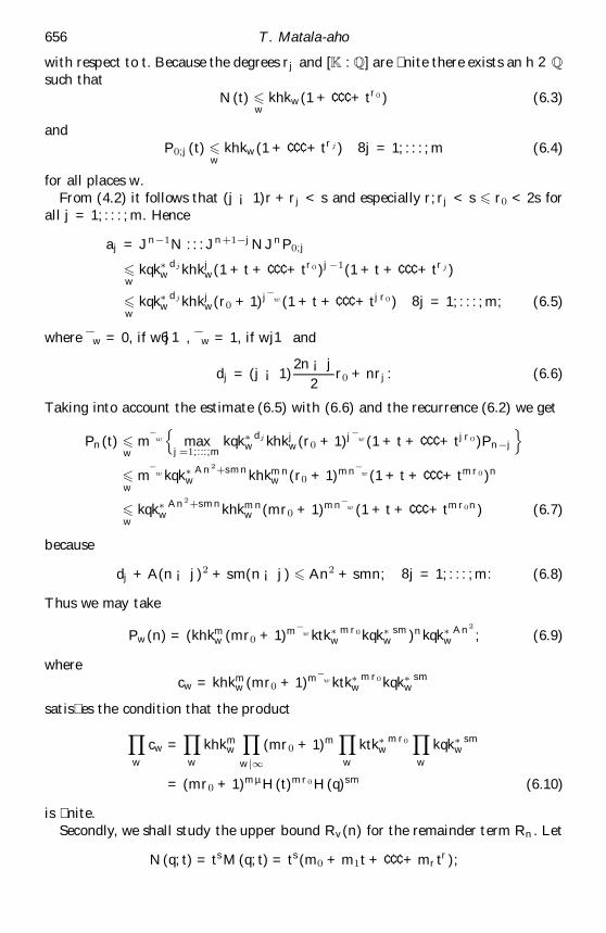
656 T. Matala-aho
with respect to t. Because the degrees rj and [K : Q] are nite there exists an h 2 Qsuch that
N (t) 6w
khkw(1 + ¢ ¢ ¢ + tr0 ) (6.3)
andP0;j(t) 6
wkhkw(1 + ¢ ¢ ¢ + trj ) 8j = 1; : : : ; m (6.4)
for all places w.From (4.2) it follows that (j ¡ 1)r + rj < s and especially r; rj < s 6 r0 < 2s for
all j = 1; : : : ; m. Hence
aj = Jn¡1N : : : Jn + 1¡jNJnP0;j
6w
kqk¤w
dj khkjw(1 + t + ¢ ¢ ¢ + tr0 )j¡1(1 + t + ¢ ¢ ¢ + trj )
6w
kqk¤w
dj khkjw(r0 + 1)j¯ w (1 + t + ¢ ¢ ¢ + tjr0 ) 8j = 1; : : : ; m; (6.5)
where ¯ w = 0, if w 6 j 1, ¯ w = 1, if wj1 and
dj = (j ¡ 1)2n ¡ j
2r0 + nrj: (6.6)
Taking into account the estimate (6.5) with (6.6) and the recurrence (6.2) we get
Pn(t) 6w
m ¯ w
nmax
j = 1;:::;mkqk ¤
wdj khkj
w(r0 + 1)j¯ w (1 + t + ¢ ¢ ¢ + tjr0 )Pn¡j
o
6w
m ¯ w kqk ¤w
An2 + smnkhkmnw (r0 + 1)mn¯ w (1 + t + ¢ ¢ ¢ + tmr0 )n
6w
kqk ¤w
An2 + smnkhkmnw (mr0 + 1)mn¯ w (1 + t + ¢ ¢ ¢ + tmr0n) (6.7)
because
dj + A(n ¡ j)2 + sm(n ¡ j) 6 An2 + smn; 8j = 1; : : : ; m: (6.8)
Thus we may take
Pw(n) = (khkmw (mr0 + 1)m¯ w ktk ¤
wmr0 kqk ¤
wsm)nkqk ¤
wAn2
; (6.9)
wherecw = khkm
w (mr0 + 1)m¯ w ktk¤w
mr0 kqk ¤w
sm
satis es the condition that the product
Y
w
cw =Y
w
khkmw
Y
wj1
(mr0 + 1)mY
w
ktk¤w
mr0Y
w
kqk ¤w
sm
= (mr0 + 1)mµ H(t)mr0 H(q)sm (6.10)
is nite.Secondly, we shall study the upper bound Rv(n) for the remainder term Rn. Let
N (q; t) = tsM (q; t) = ts(m0 + m1t + ¢ ¢ ¢ + mrtr);

Diophantine approximations 657
then
jRnjv = jts(n+ 1)qs(n+12 )jv jF (tqn+ m)jv
nY
k = 0
jm0 + m1tqk + ¢ ¢ ¢ + mrtrqrkjv : (6.11)
So
jRnjv 6 jtjs(n + 1)v jqjs(
n+12 )
v c12cn11jm0jnv (6.12)
for some c12 > 0 because the product
nY
k = 0
¯̄¯̄1 +
m1tqk + ¢ ¢ ¢ + mrtrqrk
m0
¯̄¯̄v
converges for every jqjv < 1 and jF (tqn + m)jv 6 cn+ m11 by the assumption (4.3).
Hence we may take
Rv(n) = cn13ktksn
v kqksn2=2v ; c13 > 0: (6.13)
In order to study the determinant condition (3.4) we start from the de nitions(3.4) and (5.5) to get
det Pn = Nn;1Nn;2 : : : Nn;m ¢ (n); (6.14)
which together with theorem 5.2 imply
¢ (n) = ( ¡ 1)(m + 1)(n+ 1)[P0;m]n + 1[N ]n : : : [N ]n¡m+ 2: (6.15)
Hence for all q, t satisfying
P0;m(q; qkt) 6= 0; N (q; qkt) 6= 0 8k 2 N
the determinant condition (3.4) is valid because ¢ (n) 6= 0 by (6.15).So, the assumptions (3.2){(3.4) are valid with
Pw(n) = cnwkqk¤
wAn2
; Rv(n) = cn1 kqkBn2
v ;
where
A = maxj = 2;:::;m
½r1;
(j ¡ 1)(s + r) + rj
2j
¾; B =
s
2:
The assumption B + ¶ A > 0 gives the dimension estimate
d > l
¡ ¶=
B
¡ ¶ A> 1 (6.16)
by theorem 3.1 and, if d = 2, then theorem 3.3 gives the measure
· =B
B + ¶ A:
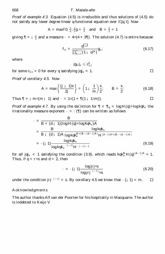
658 T. Matala-aho
Proof of example 4.3. Equation (4.5) is irreducible and thus solutions of (4.5) donot satisfy any lower degree linear q-functional equation over K[q; t]. Now
A = maxf0; 34 ; 2
3g = 3
4 and B = 22 = 1
giving ¶ > ¡ 43 and a measure · = 4=(4 + 3 ¶ ). The solution (4.7) is entire because
fn =q(n
2)Qn+ 1
k = 1(1 ¡ q2k)gn; (6.17)
wherejgnjv 6 cn
14
for some c14 > 0 for every q satisfying jqjv < 1.
Proof of corollary 4.5. Now
A = max
½(j ¡ 1)s
2j
¾=
µ1 ¡ 1
m
¶s
2; B =
s
2: (6.18)
Thus ¶ > ¡ m=(m ¡ 1) and · = 1=(1 + ¶ (1 ¡ 1=m)).
Proof of example 4.7. By using the de nition for ¶ = ¶ q = log H(q)= log kqkv theirrationality measure exponent · = · ( ¶ ) can be written as follows
· =B
B + (d ¡ 1)(log H(q)= log kqkv)A
=B
B ¡ (d ¡ 1)A
log kqkv
log kqkB=(B¡(d¡1)A)v H (d¡1)A=(B¡(d¡1)A)
= · ( ¡ 1)log kqkv
log kqkv· (¡1)
H · (¡1)¡1(6.19)
for all jqjv < 1 satisfying the condition (3.9), which reads kqkBv H(q)(d¡1)A < 1.
Thus, if q = r=s and d = 2, then
· = · ( ¡ 1)log jrj=s
log jrj· (¡1)=s
(6.20)
under the condition jrj · (¡1) < s. By corollary 4.5 we know that · ( ¡ 1) = m.
Acknowledgments
The author thanks Alf van der Poorten for his hospitality in Macquarie. The authoris indebted to Keijo V�a�an�anen and the anonymous referee for their suggestions.
References
1 M. Amou, M. Katsudara and K. V�a�an�anen. Arithmetical properties of the values of func-tions satisfying certain functional equations of Poincar¶e. Seminar on Mathematical Sciences,vol. 27, pp. 111{122 (Keio University, 1999).
2 J.-P. B¶ezivin. Independance lineaire des valeurs des solutions trascendantes de certainesequations fonctionnelles. Manuscr. Math. 61 (1988), 103{129.

Diophantine approximations 659
3 J.-P. B¶ezivin. Ind¶ependance lin¶eaire des valeurs des solutions trascendantes de certaines¶equations fonctionnelles. II. Acta Arithm. 55 (1990), 233{240.
4 P. Bundschuh. Ein Satz �uber ganze Funktionen und Irrationalit�atsaussagen. Invent. Math.9 (1970), 175{184.
5 P. Bundschuh and K. V�a�an�anen. Arithmetical investigations of a certain in¯nite product.Compositio Math. 91 (1994), 175{199.
6 V. G. Chirskii. On arithmetical properties of series. Moscow Univ. Math. Bull. 52 (1997),35{37.
7 D. Duverney. Propri¶etes des solutions de certaines ¶equations fonctionnelles de Poincar¶e. J.Th. Nombres Bordeaux 8 (1996), 443{447.
8 N. I. Fel’ dman and Yu. V. Nesterenko. Transcendental numbers. In Number theory IV (ed.A. N. Parshin and I. R. Shafarevich) (Springer, 1998).
9 M. Katsudara. Linear independence measures for values of Heine series. Math. Annln 284(1989), 449{460.
10 T. Matala-Aho. On Diophantine approximations of the Rogers{Ramanujan continued frac-tion. J. Number Theory 45 (1993), 215{227.
11 T. Matala-Aho. On the irrationality ofP 1
l = 0 dl=Q l
j = 1(1 + dj r + d2j s). Math. Univ. Oulu
(1998). Preprint.
12 T. Matala-Aho. On the values of continued fractions: q-series. Math. Univ. Oulu (2001).Preprint.
13 T. Matala-aho and K. V�a�an�anen. On approximation measures of q-logarithms. Bull. Aus-tral. Math. Soc. 58 (1998), 15{31.
14 T. Matala-aho and K. V�a�an�anen. On Diophantine approximations of mock theta functionsof third order. Ramanujan J. 4 (2000), 13{28.
15 C. F. Osgood. On the Diophantine approximation of values of functions satisfying certainlinear q-di® erence equations. J. Number Theory 3 (1971), 159{177.
16 A. Yu. Popov. Approximation of values of some in¯nite products (in Russian). VestnikMoscov. Univ. Ser. I Mat. Mekh. 6 (1990), 3{6. (English transl. Moscow Univ. Math. Bull.45 (1990), 4{6.)
17 I. Shiokawa. Rational approximations to the Rogers{Ramanujan continued fraction. ActaArithm. 50 (1988), 23{30.
18 Th. Stihl. Irrationalit�atsmasse f �ur Werte der L�osungen einer Funktionalgleichung vonPoincar¶e. Arch. Math. 41 (1983), 531{537.
19 Th. Stihl. Arithmetische Eigenschaften spezieller Heinescher Reihen. Math. Annln 268(1984), 21{41.
20 Th. Stihl and R. Wallisser. Zur Irrationalit�at und linearen Unabh�angigkeit der Werte derL�osungen einer Funktionalgleichung von Poincar¶e. J. Reine Angew. Math. 341 (1983),98{110.
21 Th. T�opfer. Arithmetical properties of functions satisfying q-di® erence equations. Analysis15 (1995), 24{49.
22 K. V�a�an�anen. On the approximation of certain in¯nite products. Math. Scand. 73 (1993),197{208
(Issued 21 June 2002 )