Chapter 4 Series Solutions and Frobenius Method

Ordinary Differential Equations (Math 6302)

A�®�Ë@ Õæ

��Aë áÖß

@ . X .

@

2017-2016 ú

GA

�JË @ É�

®Ë@

Chapter 4Series Solutions and Frobenius Method

Finding the general solution of a linear differential equation depends on determining a funda-mental set of solutions of the homogeneous equation. So far, we have given a systematic procedurefor constructing fundamental solutions in terms of of known elementary functions when the equationhas constant coefficients. To find fundamental solutions for equations with variable coefficients it isnecessary to seek other means of expression for the solutions of these equations. The principal toolthat we need is the representation of a given function by a power series. The basic idea is to assumethat the solutions of a given differential equation have power series expansions, and then we attemptto determine the coefficients so as to satisfy the differential equation.

4.1 Ordinary and Singular Points

Consider an nth-order linear equation

y(n) + a1(t)y(n−1) + · · ·+ an(t)y = 0, (1)

where y = y(t) is an unknown scalar function and a1(t), · · · , an(t) are real-valued functions and thatare continuous functions on an interval I = (r1, r2).

As we have seen before, for any t0 ∈ I and constants y0, y0, · · · , y(n−1)0 , there exists a uniquesolution y = y(t) of equation (1), which is defined on I and satisfies the initial conditions

y(t0) = y0, y(t0) = y0, · · · , y(n−1)(t0) = y(n−1)0 .

However, in many applications the coefficients will have points of discontinuity and one of themain questions is the behavior of the solutions near these points. This will be our topic.

Definition. (Analytic function)We say that a function f(t) is analytic at t = t0 if it can be expanded as a sum of a power series ofthe form

f(x) =∞∑n=1

fn (t− t0)n

with a radius of convergence R > 0.

Definition. (Ordinary and singular points of an nth-order linear equation)

(1) A point t0 is called an ordinary point of the differential equation (1) if a1(t), · · · , an(t) areanalytic at t = t0. Otherwise t = t0 is called a singular point or singularity of the equation.

1

Ordinary Differential Equations (Math 6302) A�®�Ë@ áÖß

@ . X .

@

(2) A singular point t = t0 of the equation (1) is called regular singular point if

(t− t0)jaj(t), j = 1, 2, . . . , n

are analytic at t = t0; otherwise it is called an irregular singular point.

Example. Find all singular points of the equation

t(t+ 1)2y′′ + (t− 2)y′ − 3ty = 0

and determine whether each one is regular or irregular.

Solution. The functions a1(t) =(t− 2)

t(t+ 1)2and a2(t) =

−3

(t+ 1)2are analytic at every t ∈ R−{0,−1}.

Thus, the singular points of the equation are t = 0 and t = −1.

The point t = 0 is a regular singular point since ta1(t) =(t− 2)

(t+ 1)2and t2a2(t) =

−3t2

(t+ 1)2are

analytic at t = 0.

The point t = −1 is an irregular singular point since (t + 1)a1(t) =(t− 2)

t(t+ 1)is not analytic at

t = −1.

Definition. (Ordinary and singular points of a linear system)

(1) A point t0 is called an ordinary point of the system

x = A(t)x

if A(t) is analytic at t = t0. Otherwise it t = t0 is called a singular point or singularity of thesystem.

(2) A singular point t = t0 of thex = A(t)x

is called regular singular point if (t − t0)A(t) is analytic at t = t0; otherwise it is called anirregular singular point.

Example. Find all singular points of the system

x = A(t)x

where

A =1

t2(t− 1)

(t 01 t− 1

).

Solution. A(t) is analytic at every t ∈ R − {0, 1}. Thus, the only singular points are t = 0 andt = 1.

tA(t) =1

t(t− 1)

(t 01 t− 1

)is not analytic at t = 0. Hence, t = 0 is an irregular singular point.

(t− 1)A(t) =1

t2

(t 01 t− 1

)is analytic at t = 1. So, t = 1 is a regular singular point.

of 29


@ . X .

@

Solution for large |t|To study the solution for large |t|, that is near ∞, we have to determine if the point t = ∞ is

ordinary or singular point. To achieve this goal we use the transformation

s =1

t,

and transform the point t = ∞ into s = 0. The natural of the point t = ∞ is the same as that ofs = 0. Under the transformation

s =1

tthe equation

x(t) = A(t)x(t)

is transformed into the equation

d

dsx(s) = − 1

s2A

(1

s

)x(s).

Thus, the equationx(t) = A(t)x(t)

has an ordinary point at t =∞ if

d

dsx(s) = − 1

s2A

(1

s

)x(s)

has an ordinary point at s = 0.

Solution of second-order equations about ordinary points

Many problems in mathematical physics lead to second-order equations of the form

y′′ + p(t)y′ + q(t)y = 0,

where p(t) and q(t) are rational functions. For this reason we will consider second-order equationsin detail.

Example. Find a series solution in powers of t of the Airy equation

y′′ − ty = 0, t ∈ R.

Solution.

y(t) = c1

[1 +

∞∑n=1

t3n

2 · 3 · · · (3n− 1)(3n)

]+ c2

[t+

∞∑n=1

t3n+1

3 · 4 · · · (3n)(3n+ 1)

].

Theorem 1. (Solution about an ordinary point)If t = t0 is an ordinary point of the equation

y′′ + p(t)y′ + q(t)y = 0,

then the general solution of the equation is given by

y(t) = c1h1(t) + c2h2(t),

where hj(t) are analytic functions at t = t0. Moreover, the radius of convergence of each seriessolution hj(t) is at least as large as the minimum of the radii of convergence of the series of p(t) andq(t).

of 29


@ . X .

@

Cauchy-Euler equations of the second order

The simplest equation with a regular singular point at t = 0 is the Cauchy-Euler equation

y′′ +p0ty′ +

q0t2y = 0, t > 0,

where p0 and q0 are constants.

In this equation a1(t) =p0t

and a2(t) =q0t2

. Thus, ta1(t) = p0 and t2a2(t) = q0 are analytic at

t = 0. The solution of the Cauchy-Euler equation is typical of solutions of all differential equationswith a regular singular point. Therefore, it is useful to to study the solutions of this equation indetail.

The transformationw(s) = y(t), s = ln(t), t > 0,

transforms the equation into the constant coefficient equation

d2w

ds2+ (p0 − 1)

dw

ds+ q0w = 0.

If t < 0, then the transformation

w(s) = y(t), s = ln(−t), t < 0,

transforms the equation into the constant coefficient equation

d2w

ds2+ (p0 − 1)

dw

ds+ q0w = 0.

The general solution of the new equation can be obtained in terms of the roots of the characteristicequation

λ2 + (p0 − 1)λ+ q0 = 0.

These roots are

λ1,2 =1

2

(1− p0 ±

√(p0 − 1)2 − 4q0

).

If λ1 6= λ2, then we have two linearly independent solutions

y1(t) = |t|λ1 , y2(t) = |t|λ2 .

If λ1 = λ2, then the two linearly independent solutions are

y1(t) = |t|λ1 , y2(t) = |t|λ2 ln |t|.

In order to turn to the general case, let us first consider first order equations.

Lemma 1. The first-order equationy′ + a1(t)y = 0

has a solution of the form

y(t) = tαh(t), h(t) =∞∑j=0

hjtj, h0 = 1

if and only if ta1(t) is an analytic function. In this case we have α = −limt→0

[ta1(t)].

of 29


@ . X .

@

Proof. Assume that p(t) = ta1(t) is analytic. Then

a1(t) =p0t

+ p1 + p2t+ · · ·

and the solution of the above equation is explicitly given by

y(t) = exp

(−∫ t

a1(s)ds

)= exp(−p0 ln(t) + c− p1t+ · · · )

= t−p0 exp(c− p1t+ · · · ).

Conversely, if y(t) = tαh(t) is a solution, then we have

ta1(t) = −ty′(t)

y(t)= −α− th′(t)

h(t)

which is analytic at t = 0.

4.2 The Frobenius Method for Second-order Equations

In this section, we will consider second-order linear equations

y′′ + p(t)y′ + q(t)y = 0.

In many applications the coefficients will have singularities and one of the main questions is thebehavior of the solutions near such a singularity.

We will assume that the equation has a regular singularity at t = 0; that is, we will assume thatthe coefficients p(t) and q(t) are of the form

p(t) = t−1∞∑j=0

pjtj, q(t) = t−2

∞∑j=0

qjtj.

We will look for a solution of the formy(t) = tαh(t),

where h(t) is analytic near t = 0 with h(0) = 1. This is the generalized power series method, orFrobenius method.

Differentiating

y(t) = tα∞∑j=0

hjtj

we have

y′(t) =∞∑j=0

(α + j)hjtj+α−1,

y′′(t) =∞∑j=0

(α + j)(α + j − 1)hjtj+α−2.

of 29


@ . X .

@

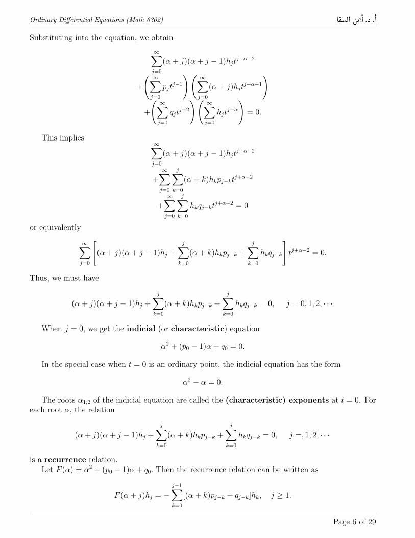
Substituting into the equation, we obtain

∞∑j=0

(α + j)(α + j − 1)hjtj+α−2

+

(∞∑j=0

pjtj−1

)(∞∑j=0

(α + j)hjtj+α−1

)

+

(∞∑j=0

qjtj−2

)(∞∑j=0

hjtj+α

)= 0.

This implies∞∑j=0

(α + j)(α + j − 1)hjtj+α−2

+∞∑j=0

j∑k=0

(α + k)hkpj−ktj+α−2

+∞∑j=0

j∑k=0

hkqj−ktj+α−2 = 0

or equivalently

∞∑j=0

[(α + j)(α + j − 1)hj +

j∑k=0

(α + k)hkpj−k +

j∑k=0

hkqj−k

]tj+α−2 = 0.

Thus, we must have

(α + j)(α + j − 1)hj +

j∑k=0

(α + k)hkpj−k +

j∑k=0

hkqj−k = 0, j = 0, 1, 2, · · ·

When j = 0, we get the indicial (or characteristic) equation

α2 + (p0 − 1)α + q0 = 0.

In the special case when t = 0 is an ordinary point, the indicial equation has the form

α2 − α = 0.

The roots α1,2 of the indicial equation are called the (characteristic) exponents at t = 0. Foreach root α, the relation

(α + j)(α + j − 1)hj +

j∑k=0

(α + k)hkpj−k +

j∑k=0

hkqj−k = 0, j =, 1, 2, · · ·

is a recurrence relation.Let F (α) = α2 + (p0 − 1)α + q0. Then the recurrence relation can be written as

F (α + j)hj = −j−1∑k=0

[(α + k)pj−k + qj−k]hk, j ≥ 1.

of 29


@ . X .

@

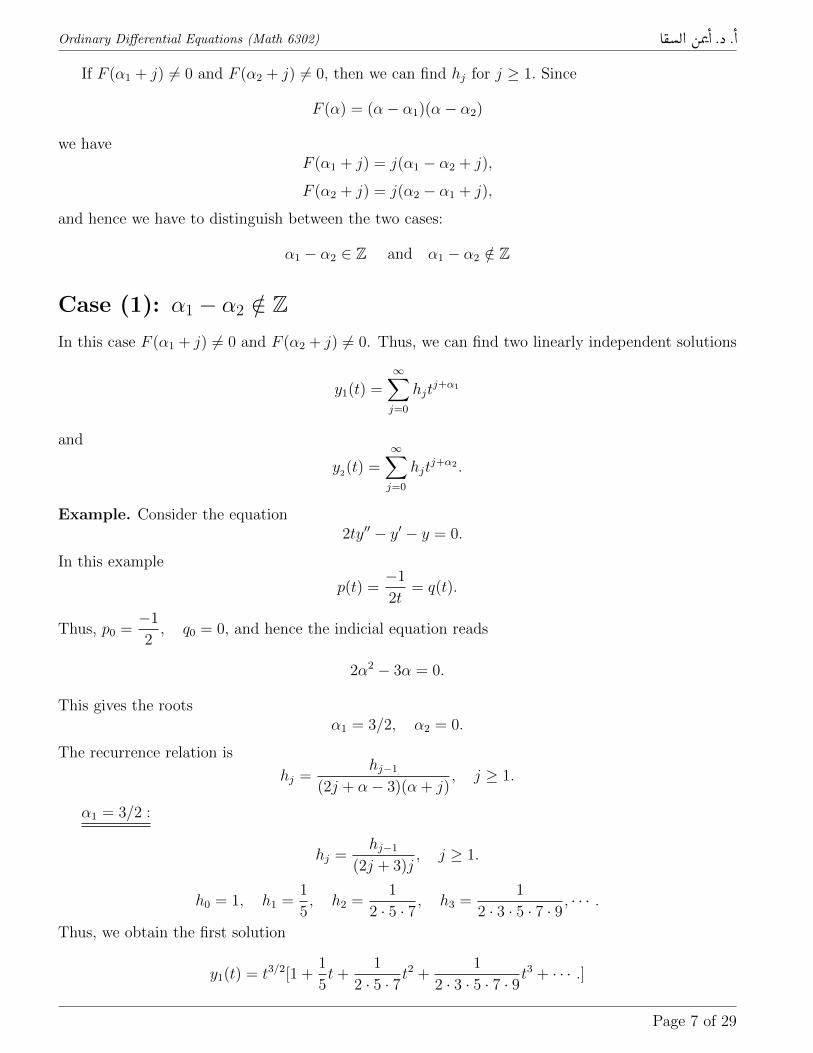
If F (α1 + j) 6= 0 and F (α2 + j) 6= 0, then we can find hj for j ≥ 1. Since

F (α) = (α− α1)(α− α2)

we haveF (α1 + j) = j(α1 − α2 + j),

F (α2 + j) = j(α2 − α1 + j),

and hence we have to distinguish between the two cases:

α1 − α2 ∈ Z and α1 − α2 /∈ Z

Case (1): α1 − α2 /∈ ZIn this case F (α1 + j) 6= 0 and F (α2 + j) 6= 0. Thus, we can find two linearly independent solutions

y1(t) =∞∑j=0

hjtj+α1

and

y2(t) =∞∑j=0

hjtj+α2 .

Example. Consider the equation2ty′′ − y′ − y = 0.

In this example

p(t) =−1

2t= q(t).

Thus, p0 =−1

2, q0 = 0, and hence the indicial equation reads

2α2 − 3α = 0.

This gives the rootsα1 = 3/2, α2 = 0.

The recurrence relation is

hj =hj−1

(2j + α− 3)(α + j), j ≥ 1.

α1 = 3/2 :

hj =hj−1

(2j + 3)j, j ≥ 1.

h0 = 1, h1 =1

5, h2 =

1

2 · 5 · 7, h3 =

1

2 · 3 · 5 · 7 · 9, · · · .

Thus, we obtain the first solution

y1(t) = t3/2[1 +1

5t+

1

2 · 5 · 7t2 +

1

2 · 3 · 5 · 7 · 9t3 + · · · .]

of 29


@ . X .

@

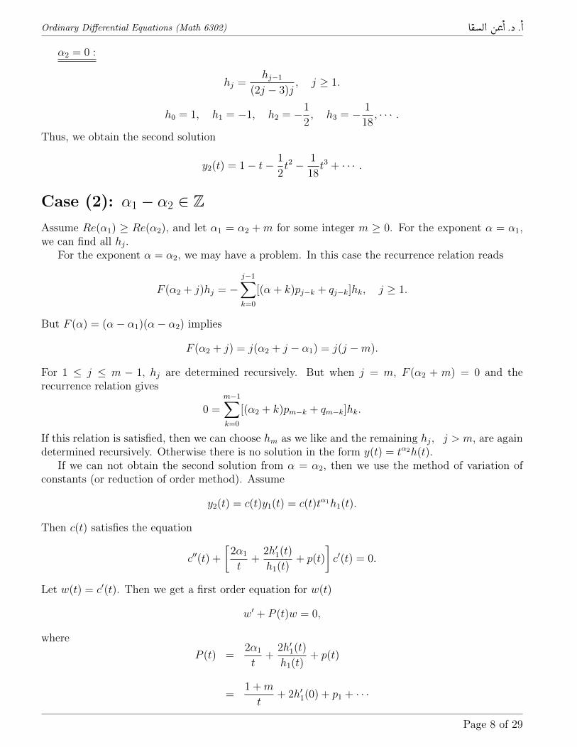
α2 = 0 :

hj =hj−1

(2j − 3)j, j ≥ 1.

h0 = 1, h1 = −1, h2 = −1

2, h3 = − 1

18, · · · .

Thus, we obtain the second solution

y2(t) = 1− t− 1

2t2 − 1

18t3 + · · · .

Case (2): α1 − α2 ∈ ZAssume Re(α1) ≥ Re(α2), and let α1 = α2 + m for some integer m ≥ 0. For the exponent α = α1,we can find all hj.

For the exponent α = α2, we may have a problem. In this case the recurrence relation reads

F (α2 + j)hj = −j−1∑k=0

[(α + k)pj−k + qj−k]hk, j ≥ 1.

But F (α) = (α− α1)(α− α2) implies

F (α2 + j) = j(α2 + j − α1) = j(j −m).

For 1 ≤ j ≤ m − 1, hj are determined recursively. But when j = m, F (α2 + m) = 0 and therecurrence relation gives

0 =m−1∑k=0

[(α2 + k)pm−k + qm−k]hk.

If this relation is satisfied, then we can choose hm as we like and the remaining hj, j > m, are againdetermined recursively. Otherwise there is no solution in the form y(t) = tα2h(t).

If we can not obtain the second solution from α = α2, then we use the method of variation ofconstants (or reduction of order method). Assume

y2(t) = c(t)y1(t) = c(t)tα1h1(t).

Then c(t) satisfies the equation

c′′(t) +

[2α1

t+

2h′1(t)

h1(t)+ p(t)

]c′(t) = 0.

Let w(t) = c′(t). Then we get a first order equation for w(t)

w′ + P (t)w = 0,

where

P (t) =2α1

t+

2h′1(t)

h1(t)+ p(t)

=1 +m

t+ 2h′1(0) + p1 + · · ·

of 29


@ . X .

@

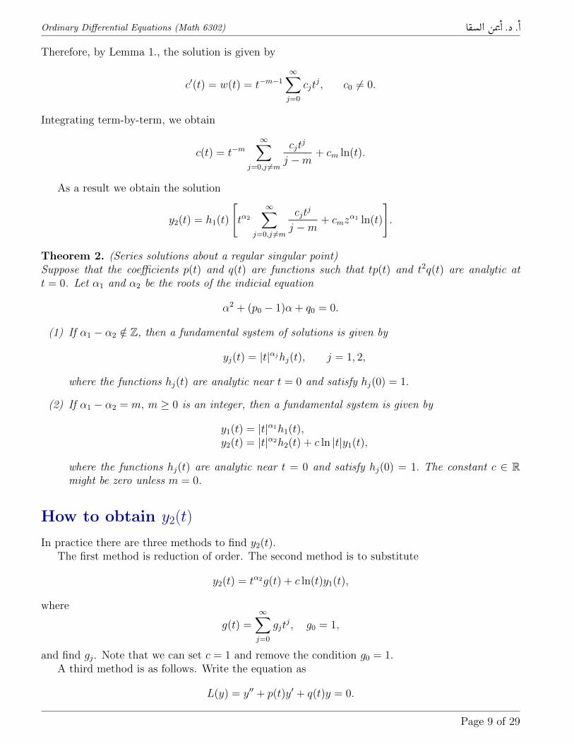
Therefore, by Lemma 1., the solution is given by

c′(t) = w(t) = t−m−1∞∑j=0

cjtj, c0 6= 0.

Integrating term-by-term, we obtain

c(t) = t−m∞∑

j=0,j 6=m

cjtj

j −m+ cm ln(t).

As a result we obtain the solution

y2(t) = h1(t)

[tα2

∞∑j=0,j 6=m

cjtj

j −m+ cmz

α1 ln(t)

].

Theorem 2. (Series solutions about a regular singular point)Suppose that the coefficients p(t) and q(t) are functions such that tp(t) and t2q(t) are analytic att = 0. Let α1 and α2 be the roots of the indicial equation

α2 + (p0 − 1)α + q0 = 0.

(1) If α1 − α2 /∈ Z, then a fundamental system of solutions is given by

yj(t) = |t|αjhj(t), j = 1, 2,

where the functions hj(t) are analytic near t = 0 and satisfy hj(0) = 1.

(2) If α1 − α2 = m, m ≥ 0 is an integer, then a fundamental system is given by

y1(t) = |t|α1h1(t),y2(t) = |t|α2h2(t) + c ln |t|y1(t),

where the functions hj(t) are analytic near t = 0 and satisfy hj(0) = 1. The constant c ∈ Rmight be zero unless m = 0.

How to obtain y2(t)

In practice there are three methods to find y2(t).The first method is reduction of order. The second method is to substitute

y2(t) = tα2g(t) + c ln(t)y1(t),

where

g(t) =∞∑j=0

gjtj, g0 = 1,

and find gj. Note that we can set c = 1 and remove the condition g0 = 1.A third method is as follows. Write the equation as

L(y) = y′′ + p(t)y′ + q(t)y = 0.

of 29


@ . X .

@

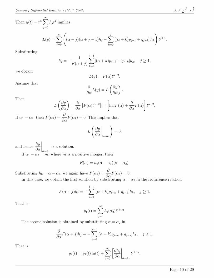
Then y(t) = tα∞∑j=0

hjtj implies

L(y) =∞∑j=0

((α + j)(α + j − 1)hj +

j∑k=0

[(α + k)pj−k + qj−k]hk

)tj+α.

Substituting

hj = − 1

F (α + j)

j−1∑k=0

[(α + k)pj−k + qj−k]hk, j ≥ 1,

we obtainL(y) = F (α)tα−2.

Assume that∂

∂αL(y) = L

(∂y

∂α

).

Then

L

(∂y

∂α

)=

∂

∂α

[F (α)tα−2

]=

[ln tF (α) +

∂

∂αF (α)

]tα−2.

If α1 = α2, then F (α1) =∂

∂αF (α1) = 0. This implies that

L

(∂y

∂α

∣∣∣∣α=α1

)= 0,

and hence∂y

∂α

∣∣∣∣α=α1

is a solution.

If α1 − α2 = m, where m is a positive integer, then

F (α) = h0(α− α1)(α− α2).

Substituting h0 = α− α2, we again have F (α2) =∂

∂αF (α2) = 0.

In this case, we obtain the first solution by substituting α = α2 in the recurrence relation

F (α + j)hj = −j−1∑k=0

[(α + k)pj−k + qj−k]hk, j ≥ 1.

That is

y1(t) =∞∑j=0

hj(α2)tj+α2 .

The second solution is obtained by substituting α = α2 in

∂

∂αF (α + j)hj = −

j−1∑k=0

[(α + k)pj−k + qj−k]hk, j ≥ 1.

That is

y2(t) = y1(t) ln(t) +∞∑j=0

[∂hj∂α

∣∣∣∣α=α2

tj+α2 .

of 29


@ . X .

@

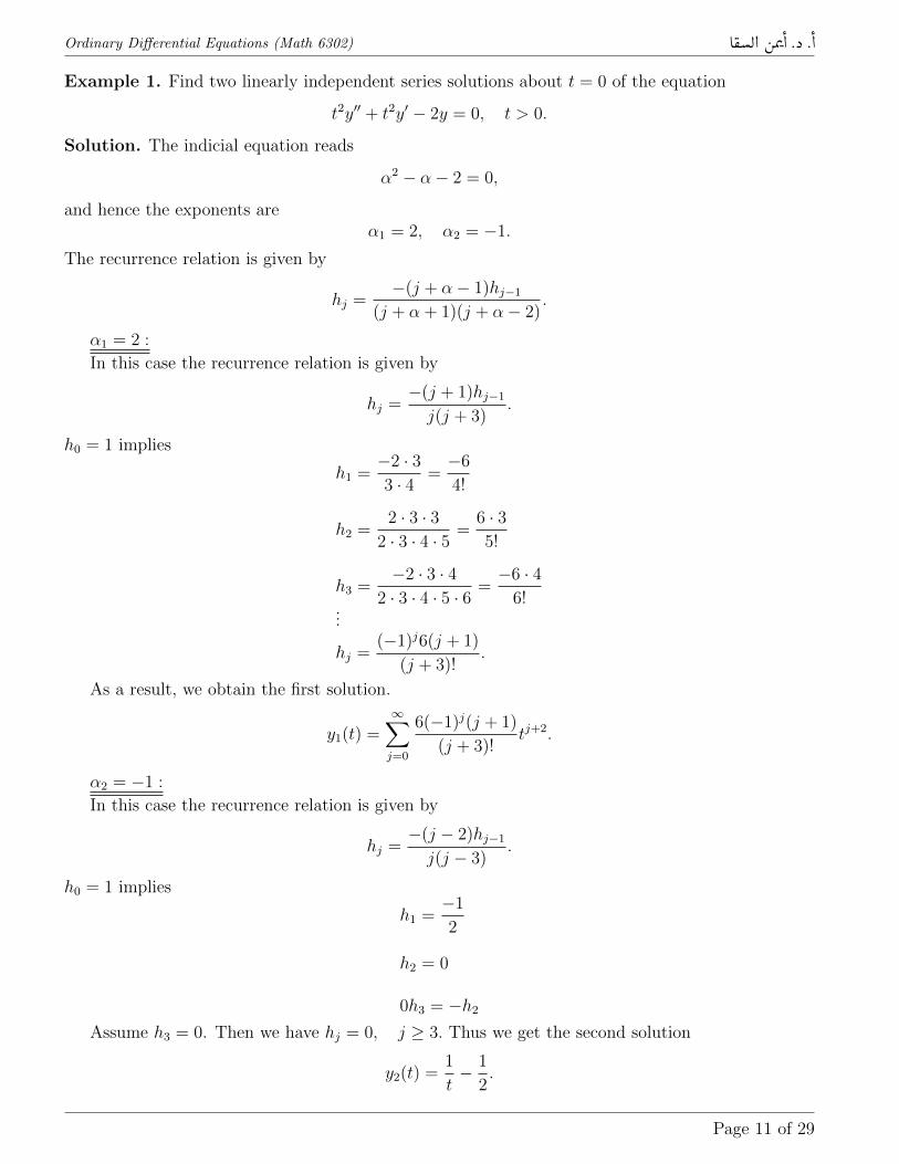
Example 1. Find two linearly independent series solutions about t = 0 of the equation

t2y′′ + t2y′ − 2y = 0, t > 0.

Solution. The indicial equation reads

α2 − α− 2 = 0,

and hence the exponents areα1 = 2, α2 = −1.

The recurrence relation is given by

hj =−(j + α− 1)hj−1

(j + α + 1)(j + α− 2).

α1 = 2 :

In this case the recurrence relation is given by

hj =−(j + 1)hj−1j(j + 3)

.

h0 = 1 implies

h1 =−2 · 33 · 4

=−6

4!

h2 =2 · 3 · 3

2 · 3 · 4 · 5=

6 · 35!

h3 =−2 · 3 · 4

2 · 3 · 4 · 5 · 6=−6 · 4

6!...

hj =(−1)j6(j + 1)

(j + 3)!.

As a result, we obtain the first solution.

y1(t) =∞∑j=0

6(−1)j(j + 1)

(j + 3)!tj+2.

α2 = −1 :

In this case the recurrence relation is given by

hj =−(j − 2)hj−1j(j − 3)

.

h0 = 1 implies

h1 =−1

2

h2 = 0

0h3 = −h2Assume h3 = 0. Then we have hj = 0, j ≥ 3. Thus we get the second solution

y2(t) =1

t− 1

2.

of 29


@ . X .

@

Example 2. Find the series solution of

t(t− 1)y′′ + (3t− 1)y′ + y = 0, t > 0,

about t = 0.

Solution. Indicial equationα2 = 0.

Thus the characteristic exponents areα1 = α2 = 0.

The recurrence relation readshj = hj−1.

The first solution is

y1(t) =1

1− t.

In order to find y2(t) let us use the method of reduction of order. Let

y2(t) = c(t)y1(t).

Differentiating we gety′2 = c′y1 + cu′1, y′′2 = c′′y1 + 2c′y′1 + cu′′1.

Substituting into the equation

t(t− 1)y′′ + (3t− 1)y′ + y = 0,

we obtaint(t− 1)(c′′y1 + 2c′y′1 + cu′′1) + (3t− 1)(c′y1 + cu′1) + cu1 = 0.

But y1 is a solution; that ist(t− 1)y′′1 + (3t− 1)y′1 + y1 = 0.

Thus, we havet(t− 1)(c′′y1 + 2c′y′1) + (3t− 1)c′y1 = 0.

This givesc′′

c′= −2y′1

y1− 3t− 1

t(t− 1).

Integrating we obtainln(c′) = −2 ln(y1)− ln(t)− 2 ln(t− 1).

This gives

c′ =1

y21t(t− 1)2=

1

t

and hencec(t) = ln(t).

Using the method of reduction of order, we find

y2(t) =ln t

1− t.

of 29


@ . X .

@

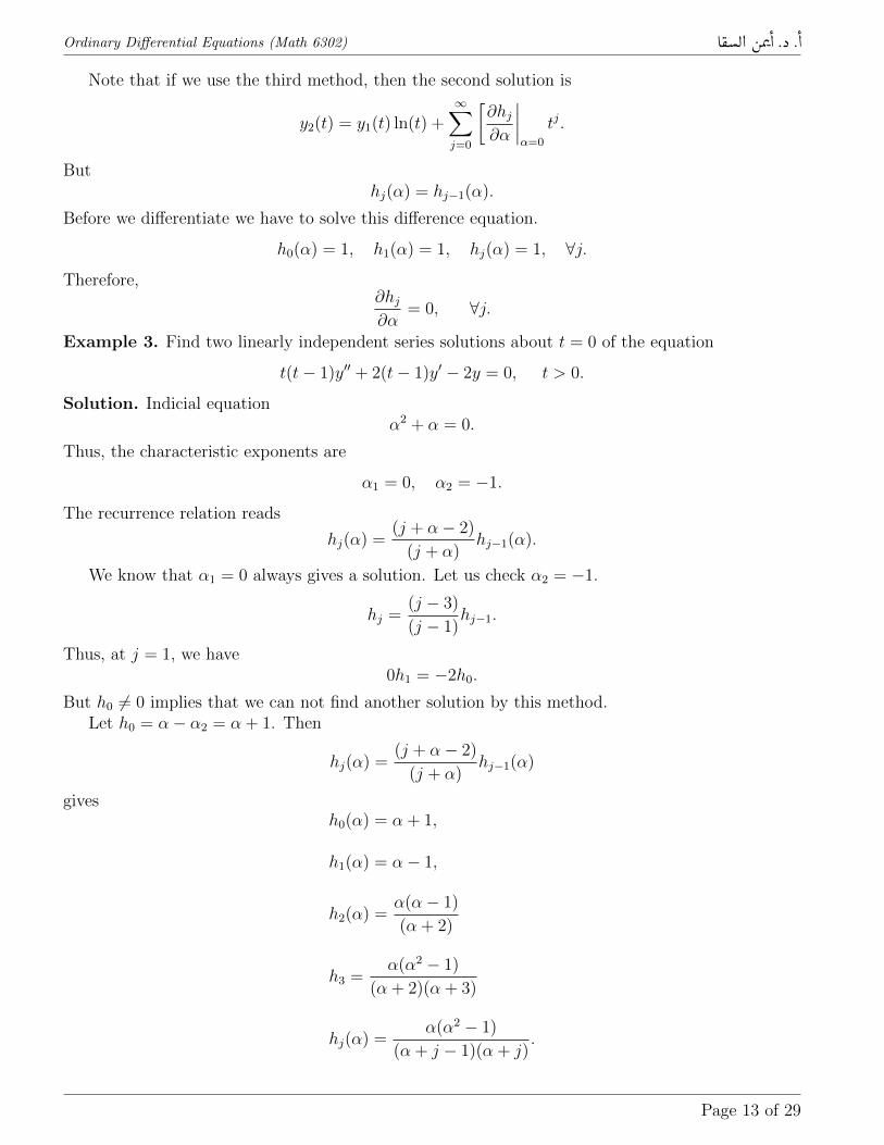
Note that if we use the third method, then the second solution is

y2(t) = y1(t) ln(t) +∞∑j=0

[∂hj∂α

∣∣∣∣α=0

tj.

Buthj(α) = hj−1(α).

Before we differentiate we have to solve this difference equation.

h0(α) = 1, h1(α) = 1, hj(α) = 1, ∀j.

Therefore,∂hj∂α

= 0, ∀j.

Example 3. Find two linearly independent series solutions about t = 0 of the equation

t(t− 1)y′′ + 2(t− 1)y′ − 2y = 0, t > 0.

Solution. Indicial equationα2 + α = 0.

Thus, the characteristic exponents are

α1 = 0, α2 = −1.

The recurrence relation reads

hj(α) =(j + α− 2)

(j + α)hj−1(α).

We know that α1 = 0 always gives a solution. Let us check α2 = −1.

hj =(j − 3)

(j − 1)hj−1.

Thus, at j = 1, we have0h1 = −2h0.

But h0 6= 0 implies that we can not find another solution by this method.Let h0 = α− α2 = α + 1. Then

hj(α) =(j + α− 2)

(j + α)hj−1(α)

givesh0(α) = α + 1,

h1(α) = α− 1,

h2(α) =α(α− 1)

(α + 2)

h3 =α(α2 − 1)

(α + 2)(α + 3)

hj(α) =α(α2 − 1)

(α + j − 1)(α + j).

of 29


@ . X .

@

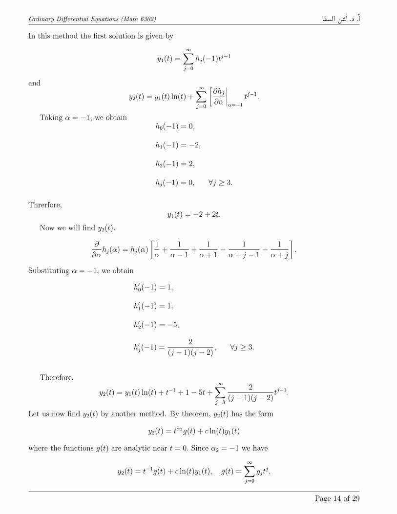
In this method the first solution is given by

y1(t) =∞∑j=0

hj(−1)tj−1

and

y2(t) = y1(t) ln(t) +∞∑j=0

[∂hj∂α

∣∣∣∣α=−1

tj−1.

Taking α = −1, we obtainh0(−1) = 0,

h1(−1) = −2,

h2(−1) = 2,

hj(−1) = 0, ∀j ≥ 3.

Threrfore,y1(t) = −2 + 2t.

Now we will find y2(t).

∂

∂αhj(α) = hj(α)

[1

α+

1

α− 1+

1

α + 1− 1

α + j − 1− 1

α + j

].

Substituting α = −1, we obtain

h′0(−1) = 1,

h′1(−1) = 1,

h′2(−1) = −5,

h′j(−1) =2

(j − 1)(j − 2), ∀j ≥ 3.

Therefore,

y2(t) = y1(t) ln(t) + t−1 + 1− 5t+∞∑j=3

2

(j − 1)(j − 2)tj−1.

Let us now find y2(t) by another method. By theorem, y2(t) has the form

y2(t) = tα2g(t) + c ln(t)y1(t)

where the functions g(t) are analytic near t = 0. Since α2 = −1 we have

y2(t) = t−1g(t) + c ln(t)y1(t), g(t) =∞∑j=0

gjtj.

of 29


@ . X .

@

If we set g0 = 1, then we choose c to satisfy this condition. Alternatively we can take c = 1 andremove the condition g0 = 1.

Let us choose g0 = 1. Differentiating, we get

y′2(t) = t−1g′(t)− t−2g(t) + c

[ln(t)y′1(t) +

1

ty1(t)

]

y′′2(t) = t−1g′′(t)− 2t−2g′(t) + 2t−3g(t) + c

[ln(t)y′′1(t) +

2

ty′1(t)−

1

t2y1(t)

]Substituting into the equation, we obtain

t(t− 1)

(t−1g′′(t)− 2t−2g′(t) + 2t−3g(t) + c

[ln(t)y′′1(t) +

2

ty1(t)−

1

t2y1(t)

])+2(t− 1)

(t−1g′(t)− t−2g(t) + c

[ln(t)y′1(t) +

1

ty1(t)

])− 2[t−1g(t) + c ln(t)y1(t)] = 0.

Substituting y1(t) = 1− t and simplifying we obtain

t(t− 1)g′′(t)− 2g = c[3t2 − 4t+ 1].

Now substituting g(t) =∞∑j=0

gjtj, we obtain c = −2

g0 = 1, g2 = −4− g1, g3 = 1,

(j − 1)gj = (j − 3)gj−1, j ≥ 4.

This gives

gj =2

(j − 1)(j − 2), j ≥ 3.

As a result we obtain

y2(t) = −2(1− t) ln(t) + t−1 + g1 − (g1 + 4)t+∞∑j=3

2

(j − 1)(j − 2)tj−1.

Example 4. Solvety′′ + y = 0, t > 0,

about t = 0

Solution. Indicial equationα2 − α = 0.

It follows that the characteristic exponents are

α1 = 1, α2 = 0.

The recurrence relation reads

hj(α) =−hj−1(α)

(j + α)(j + α− 1).

of 29


@ . X .

@

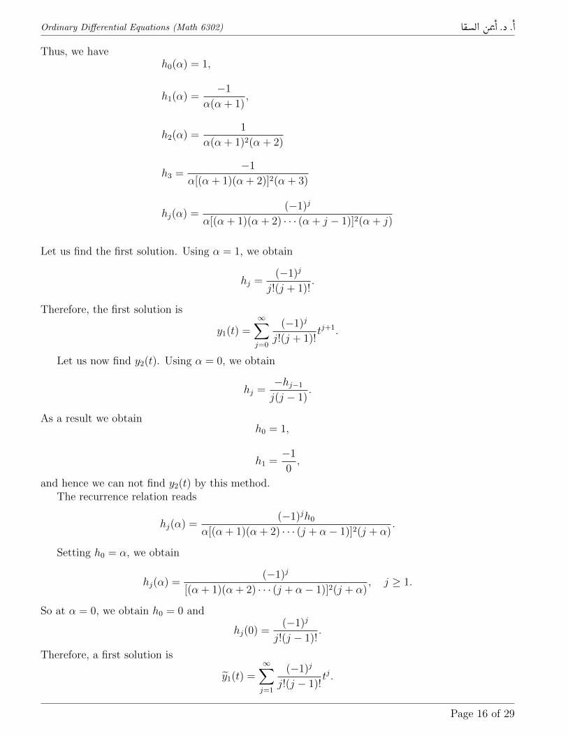
Thus, we haveh0(α) = 1,

h1(α) =−1

α(α + 1),

h2(α) =1

α(α + 1)2(α + 2)

h3 =−1

α[(α + 1)(α + 2)]2(α + 3)

hj(α) =(−1)j

α[(α + 1)(α + 2) · · · (α + j − 1)]2(α + j)

Let us find the first solution. Using α = 1, we obtain

hj =(−1)j

j!(j + 1)!.

Therefore, the first solution is

y1(t) =∞∑j=0

(−1)j

j!(j + 1)!tj+1.

Let us now find y2(t). Using α = 0, we obtain

hj =−hj−1j(j − 1)

.

As a result we obtainh0 = 1,

h1 =−1

0,

and hence we can not find y2(t) by this method.The recurrence relation reads

hj(α) =(−1)jh0

α[(α + 1)(α + 2) · · · (j + α− 1)]2(j + α).

Setting h0 = α, we obtain

hj(α) =(−1)j

[(α + 1)(α + 2) · · · (j + α− 1)]2(j + α), j ≥ 1.

So at α = 0, we obtain h0 = 0 and

hj(0) =(−1)j

j!(j − 1)!.

Therefore, a first solution is

y1(t) =∞∑j=1

(−1)j

j!(j − 1)!tj.

of 29


@ . X .

@

Now we will find

y2(t) = y1(t) ln(t) +∞∑j=0

[∂hj∂α

∣∣∣∣α=0

tj.

Firstly, h′0 = 1. Using logarithmic differentiation we get

∂hj∂α

∣∣∣∣α=0

= −hj(0)

[1

j+ 2

j−1∑k=1

1

k

], j ≥ 1.

Using the harmonic numbers

Hj =

j∑k=1

1

k,

we have∂hj∂α

∣∣∣∣α=0

=(−1)j+1

j!(j − 1)![Hj +Hj−1] , j ≥ 1.

As a result, we obtain

y2(t) = y1(t) ln(t) + 1 + t+∞∑j=2

(−1)j+1

j!(j − 1)![Hj +Hj−1] t

j.

Exercises

Find two linearly independent series solutions about t = 0 (t > 0) for each of the following equations:

1. 2t(t+ 1)y′′ + 3(t+ 1)y′ − y = 0.

2. 4t2y′′ + 4ty′ − (4t2 + 1)y = 0.

3. 2ty′′ + (2t+ 1)y′ − 5y = 0.

4. t2y′′ − t(t+ 1)y′ + y = 0.

5. 4t2y′′ − (2t− 1)y = 0.

6. t2y′′ + 2t(t− 21)y′ − 2(3t− 2)y = 0.

7. t2y′′ + t(3t+ 2)y′ − 2y = 0.

8. 2ty′′ + 6y′ + y = 0.

9. t2y′′ − 3ty′ + (4t+ 3)y = 0.

10. ty′′ + y′ + ty = 0.

4.3 Special Functions

Special functions are particular mathematical functions which have more or less established namesand notations due to their importance in mathematical analysis, functional analysis, physics, orother applications. Many special functions appear as solutions of differential equations or integralsof elementary functions.

of 29


@ . X .

@

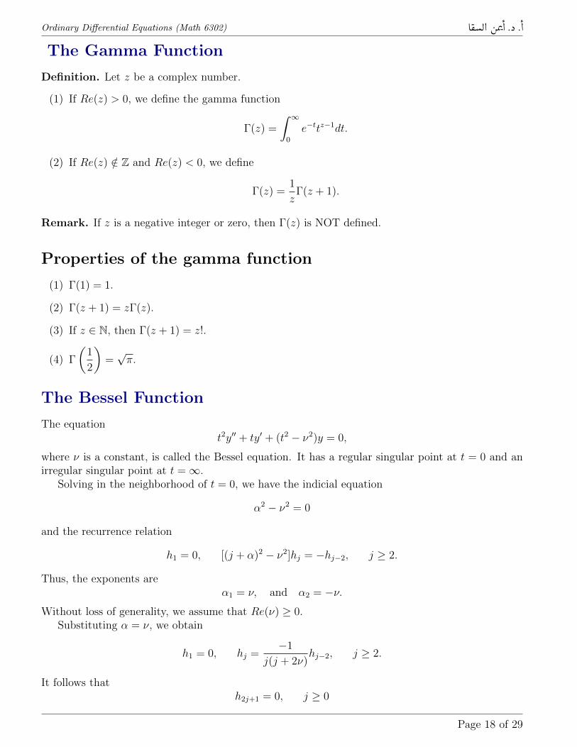
The Gamma Function

Definition. Let z be a complex number.

(1) If Re(z) > 0, we define the gamma function

Γ(z) =

∫ ∞0

e−ttz−1dt.

(2) If Re(z) /∈ Z and Re(z) < 0, we define

Γ(z) =1

zΓ(z + 1).

Remark. If z is a negative integer or zero, then Γ(z) is NOT defined.

Properties of the gamma function

(1) Γ(1) = 1.

(2) Γ(z + 1) = zΓ(z).

(3) If z ∈ N, then Γ(z + 1) = z!.

(4) Γ

(1

2

)=√π.

The Bessel Function

The equationt2y′′ + ty′ + (t2 − ν2)y = 0,

where ν is a constant, is called the Bessel equation. It has a regular singular point at t = 0 and anirregular singular point at t =∞.

Solving in the neighborhood of t = 0, we have the indicial equation

α2 − ν2 = 0

and the recurrence relation

h1 = 0, [(j + α)2 − ν2]hj = −hj−2, j ≥ 2.

Thus, the exponents areα1 = ν, and α2 = −ν.

Without loss of generality, we assume that Re(ν) ≥ 0.Substituting α = ν, we obtain

h1 = 0, hj =−1

j(j + 2ν)hj−2, j ≥ 2.

It follows thath2j+1 = 0, j ≥ 0

of 29


@ . X .

@

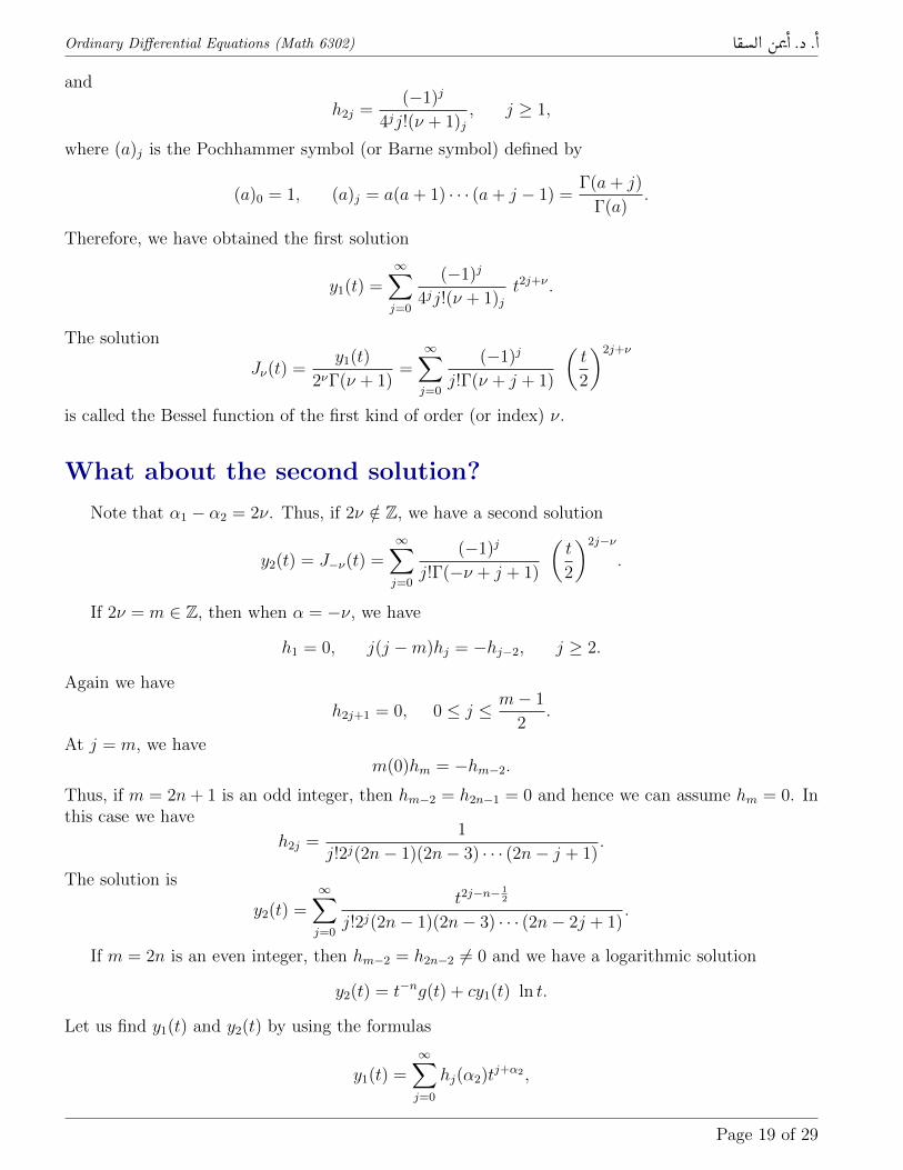
and

h2j =(−1)j

4jj!(ν + 1)j, j ≥ 1,

where (a)j is the Pochhammer symbol (or Barne symbol) defined by

(a)0 = 1, (a)j = a(a+ 1) · · · (a+ j − 1) =Γ(a+ j)

Γ(a).

Therefore, we have obtained the first solution

y1(t) =∞∑j=0

(−1)j

4jj!(ν + 1)jt2j+ν .

The solution

Jν(t) =y1(t)

2νΓ(ν + 1)=∞∑j=0

(−1)j

j!Γ(ν + j + 1)

(t

2

)2j+ν

is called the Bessel function of the first kind of order (or index) ν.

What about the second solution?

Note that α1 − α2 = 2ν. Thus, if 2ν /∈ Z, we have a second solution

y2(t) = J−ν(t) =∞∑j=0

(−1)j

j!Γ(−ν + j + 1)

(t

2

)2j−ν

.

If 2ν = m ∈ Z, then when α = −ν, we have

h1 = 0, j(j −m)hj = −hj−2, j ≥ 2.

Again we have

h2j+1 = 0, 0 ≤ j ≤ m− 1

2.

At j = m, we havem(0)hm = −hm−2.

Thus, if m = 2n+ 1 is an odd integer, then hm−2 = h2n−1 = 0 and hence we can assume hm = 0. Inthis case we have

h2j =1

j!2j(2n− 1)(2n− 3) · · · (2n− j + 1).

The solution is

y2(t) =∞∑j=0

t2j−n−12

j!2j(2n− 1)(2n− 3) · · · (2n− 2j + 1).

If m = 2n is an even integer, then hm−2 = h2n−2 6= 0 and we have a logarithmic solution

y2(t) = t−ng(t) + cy1(t) ln t.

Let us find y1(t) and y2(t) by using the formulas

y1(t) =∞∑j=0

hj(α2)tj+α2 ,

of 29


@ . X .

@

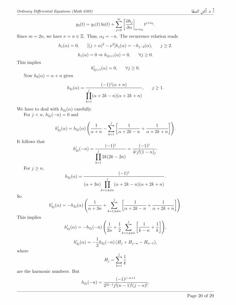
y2(t) = y1(t) ln(t) +∞∑j=0

[∂hj∂α

∣∣∣∣α=α2

tj+α2 .

Since m = 2n, we have ν = n ∈ Z. Thus, α2 = −n. The recurrence relation reads

h1(α) = 0, [(j + α)2 − ν2]hj(α) = −hj−2(α), j ≥ 2.

h1(α) = 0⇒ h2j+1(α) = 0, ∀j ≥ 0.

This impliesh′2j+1(α) = 0, ∀j ≥ 0.

Now h0(α) = α + n gives

h2j(α) =(−1)j(α + n)

j∏k=1

(α + 2k − n)(α + 2k + n)

, j ≥ 1.

We have to deal with h2j(α) carefully.For j < n, h2j(−n) = 0 and

h′2j(α) = h2j(α)

(1

α + n−

j∑k=1

[1

α + 2k − n+

1

α + 2k + n

]).

It follows that

h′2j(−n) =(−1)j

j∏k=1

2k(2k − 2n)

=(−1)j

4jj!(1− n)j.

For j ≥ n,

h2j(α) =(−1)j

(α + 3n)

j∏k=1,k 6=n

(α + 2k − n)(α + 2k + n)

.

So

h′2j(α) = −h2j(α)

(1

α + 3n+

j∑k=1,k 6=n

[1

α + 2k − n+

1

α + 2k + n

]).

This implies

h′2j(α) = −h2j(−n)

(1

2n+

1

2

j∑k=1,k 6=n

[1

k − n+

1

k

]),

h′2j(α) = −1

2h2j(−n) (Hj +Hj−n −Hn−1),

where

Hj =

j∑k=1

1

k

are the harmonic numbers. But

h2j(−n) =(−1)j−n+1

22j−1j!(n− 1)!(j − n)!.

of 29


@ . X .

@

Therefore,

h′2j(α) =(−1)j−n

22jj!(n− 1)!(j − n)!(Hj +Hj−n −Hn−1),

and hence

y1(t) =∞∑j=n

(−1)j−n+1t2j−n

22j−1j!(n− 1)!(j − n)!

=∞∑j=0

(−1)j+1t2j+n

22j+2n−1j!(n− 1)!(j + n)!

=−Jn(t)

2n−1(n− 1)!.

The second solution is

y2(t) = y1(t) ln(t) +n−1∑j=0

(−1)jt2j−n

4jj!(1− n)j+∞∑j=n

(−1)j−n (Hj +Hj−n −Hn−1) t2j−n

22jj!(n− 1)!(j − n)!

= y1(t) ln(t) +n−1∑j=0

(−1)jt2j−n

4jj!(1− n)j+∞∑j=0

(−1)j (Hj +Hj+n −Hn−1) t2j+n

22j+2nj!(n− 1)!(j + n)!

= y1(t) ln(t) +n−1∑j=0

(−1)jt2j−n

4jj!(1− n)j−Hn−1

∞∑j=0

(−1)jt2j+n

22j+2nj!(n− 1)!(j + n)!

+∞∑j=0

(−1)j (Hj +Hj+n) t2j+n

22j+2nj!(n− 1)!(j + n)!

= y1(t) ln(t) +n−1∑j=0

(−1)jt2j−n

4jj!(1− n)j+

1

2Hn−1y1(t) +

∞∑j=0

(−1)j (Hj +Hj+n) t2j+n

22j+2nj!(n− 1)!(j + n)!.

The linear combination

Yn(t) =−2n(n− 1)!

π

[(γ − ln(2)− 1

2Hn−1)y1(t) + y2(t)

]gives the new solution

Yn(t) =2

π[γ + ln

(t

2

)]Jn(t)− 1

π

n−1∑j=1

(−1)j(n− 1)!

j!(1− n)j

(t

2

)2j−n

− 1

π

∞∑j=0

(−1)j (Hj +Hj+n)

j!(j + n)!

(t

2

)2j+n

,

where γ = limj→∞

[Hj − ln(j)] is the Euler constant. Yn(t) is called the Bessel’s function of the second

kind of order n or the Neumann’s function.Note that Yν(t) can be defined as

Yν(t) =cos(πν)Jν(t)− J−ν(t)

sin(νπ).

Properties of the Bessel function

(1)d

dt(t±νJν(t)) = ±t±νJν∓1(t).

of 29


@ . X .

@

(2) Jν+1(t) + Jν−1(t) =2ν

tJν(t).

(2) Jν+1(t)− Jν−1(t) = 2J ′ν(t).

Proof. (1)d

dt(tνJν(t)) = tνJ ′ν(t) + νtν−1Jν(t)

Jν(t) =∞∑j=0

(−1)j

j!Γ(ν + j + 1)

(t

2

)2j+ν

⇒ J ′ν(t) =∞∑j=0

(−1)j(2j + ν)

2j!Γ(ν + j + 1)

(t

2

)2j+ν−1

⇒ tJ ′ν(t) + νJν(t) =∞∑j=0

(−1)j(2j + 2ν)

j!Γ(ν + j + 1)

(t

2

)2j+ν

.

UsingΓ(x+ 1) = xΓ(x)

we obtain

tJ ′ν(t) + νJν(t) =∞∑j=0

2(−1)j

j!Γ(ν + j)

(t

2

)2j+ν

= tJν−1(t).

The Legendre Function

The equation(1− t2)y′′ − 2ty′ + n(n+ 1)y = 0

is called the Legendre differential equation. It has regular singular points at t = 1,−1,∞.Solving in the neighborhood of t =∞, we have the indicial equation

α2 + α− n(n+ 1) = 0

and the recurrence relation

h1 = 0, (α− n− j)(α + n+ 1− j)hj = (α− j + 1)(α− j + 2)hj−2, j ≥ 2.

Thus, the exponents areα1 = n, and α2 = −(n+ 1).

Substituting α = n, we obtain

h1 = 0, j(j − 2n− 1)hj = (j − n− 1)(j − n− 2)hj−2, j ≥ 2.


and

h0 = 1, h2j =(−n)(−n+ 1)(−n+ 2) . . . (−n+ 2j − 1)

j! 2j (−2n+ 1)(−2n+ 3) . . . (−2n+ 2j − 1), j ≥ 1.

of 29


@ . X .

@

Note that h2j can be written as

h2j =(−n

2)j (1

2− n

2)j

j!(12− n)j

, j ≥ 0.

Thus, a first solution is

y1(t) =∞∑j=0

(−n2)j (1

2− n

2)j

j!(12− n)j

tn−2j.

If α1 − α2 = 2n+ 1 /∈ Z, then substituting α = −(n+ 1), we obtain

h1 = 0, j(j − 2n− 1)hj = (j + n− 1)(j + n)hj−2, j ≥ 2.


and

h2j =(n+ 1)(n+ 2) . . . (n+ 2j − 1)(n+ 2j)

j! 2j (−2n+ 3)(−2n+ 5) . . . (−2n+ 2j + 1), j ≥ 1.

Thus, a second solution solution is

y2(t) = t−n−1 +∞∑j=1

(n+ 1)(n+ 2) . . . (n+ 2j − 1)(n+ 2j)

j! 2j (−2n+ 3)(−2n+ 5) . . . (−2n+ 2j + 1)t−n−2j−1.

Legendre Polynomials

If n is a nonnegative integer, then the solution y1(t) of the Legendre’s equation is a polynomial.Indeed if n is a nonnegative integer, then h2j can be written as

h2j =(−1)jn(n− 1)(n− 2) . . . (n− 2j + 1)

j! 2j (2n− 1)(2n− 3) . . . (2n− 2j + 1), j ≥ 1.

But

n(n− 1)(n− 2) . . . (n− 2j + 1) =n!

(n− 2j)!

and

(2n− 1)(2n− 3) . . . (2n− 2j + 1) =(2n)!(n− j)!

2jn!(2n− 2j)!.

Thus, y1(t) can be written as

y1(t) =

[n/2]∑j=0

(−1)j(n!)2(2n− 2j)!

(2n)! j! (n− j)! (n− 2j)!tn−2j,

where [n/2] is the greatest integer less than or equal to n/2.

The Legendre polynomials Pn(t) =(2n)!

2n(n!)2y1(t) are given by

Pn(t) =1

2n

[n/2]∑j=0

(−1)j(2n− 2j)!

j!(n− j)!(n− 2j)!tn−2j.

P0(t) = 1, P1(t) = t, P2(t) =1

2(3t2 − 1), P3(t) =

1

2t(5t− 3), · · · .

of 29


@ . X .

@

Properties of the Legendre function

(1) Pn(1) = 1.

(2) Pn(−1) = (−1)n.

(3) Pn(−t) = (−1)nPn(t).

(4) (n+ 1)Pn+1(t)− (2n+ 1)tPn(t) + nPn−1(t) = 0, n ∈ N.

(5) tP ′n(t)− P ′n−1(t) = nPn(t).

(6) P ′n+1 = tP ′n(t) + (n+ 1)Pn(t).

(7) Pn(t) =1

2nn!

dn

dtn[(t2 − 1)n], n = 0, 1, 2, · · · .

(8) (1− 2tx+ x2)−1/2 =∞∑n=0

Pn(t)xn.

The Hypergeometric Function

Let us consider the hypergeometric equation

t(1− t)y′′ + [c− (1 + a+ b)t]y′ − ab y = 0,

where a, b, c are complex parameters. It has regular singularities at 0, 1, ∞, and hence it is aFuchsian equation. The exponents of these singularities are as follows:

(1) t = 0: exponents 0 and 1− c.

(2) t = 1: exponents 0 and c− a− b.

(3) t =∞: exponents a and b.

All these information are symbolically represented by

y = P

0 1 ∞0 0 a t

1− c c− a− b b

.

P is called the Riemann-P-function.

Solution in the neighborhood of t = 0

Let us look for solutions

u(t) =∞∑j=0

hjtj+α

in the neighborhood of t = 0. The exponents are α1 = 0 and α2 = 1− c and the recurrence relationreads

(j + α)(j + α + c− 1)hj = (j + α + a− 1)(j + α + b− 1)hj−1, j ≥ 1.

of 29


@ . X .

@

A first solution can obtained if we substitute α = α1 = 0. In this case the recurrence relationbecomes

hj =(j + a− 1)((j + b− 1)

j(j + c− 1)hj−1, j ≥ 1.

Thus, if 1− c /∈ N, then we have

hj =(a)j(b)jj!(c)j

,

where (a)j is the Pochhammer symbol. As a result we obtain the solution

y1(t) =∞∑j=0

(a)j(b)jj!(c)j

tj.

This function is called the hypergeometric function and it is denoted by F (a, b, c; t) or 2F1(a, b, c; t).

Remark. Many familiar functions are special cases of the hypergeometric function. For example

• sin−1 t = tF (1

2,1

2,3

2; t2),

• tan−1 t = tF (1

2, 1,

3

2;−t2),

• (1− t)n = F (−n, 1, 1; t).

Properties of the hypergeometric function

(1) F (a, b, c; 0) = 1.

(2)d

dzF (a, b, c : t) =

ab

cF (a+ 1.b+ 1, c+ 1 : t).

(3)d

dzF (a, b, c : t)

∣∣∣∣t=0

=ab

c.

(4) (a− b)F (a, b, c; t) = aF (a+ 1, b, c; t)− bF (a, b+ 1, c, t).

Second solution

Let y(t) = t1−cw(t). Then w(t) satisfies the hypergeometric equation

t(1− t)w′′ + [γ − (1 + α + β)t]w′ − αβ w = 0,

where α = a− c+ 1, β = b− c+ 1, γ = 2− c. We know that if 1− γ = −1 + c /∈ N, then

w(t) = F (α, β, γ; t)

is a solution of this equation. Hence

y2(t) = t1−cF (a− c+ 1, b− c+ 1, 2− c; t)

is a second solution of the hypergeometric equation provided that c /∈ Z. It can be shown that y1(t)and y2(t) are linearly independent.

of 29


@ . X .

@

Exercises

(1) Prove the following:

(a) Γ(1) = 1.

(b) Γ(z + 1) = zΓ(z).

(c) If z ∈ N, then Γ(z + 1) = z!.

(d) Γ

(1

2

)=√π.

(2) Find two linearly independent series solutions of the Hermite equation

y′′ − 2ty′ + 2nu = 0, n ∈ R.

(3) Find two linearly independent series solutions of the Confluent Hypergeometric equation

ty′′ + (c− t)y′ − au = 0, a, c ∈ R.

(4) Find two linearly independent series solutions of the Lagurre equation

ty′′ + (1− t)y′ + nu, n ∈ R.

(5) Show that the general solution of the Chebyshev differential equation

(1− t2)y′′ − ty′ + a2x = 0, a ∈ R

is given by

y(t) = c0

[1 +

∞∑n=1

(−a)2(22 − a2) . . . ((2n− 2)2 − a2)(2n)!

t2n

]

+c1

[t+

∞∑n=1

(1− a2)(32 − a2) . . . ((2n− 1)2 − a2)(2n− 1)!

t2n+1

].

4.4 The Frobenius Method for Systems

In this section we will consider linear systems

x′ = A(t)x.

Assume that the systemx′ = A(t)x

has a regular singular point at t = 0; that is assume that

A(t) =1

t

∞∑j=0

Ajtj.

Then we will look for solution of the system in the form

x(t) = tαU(t), U(t) =∞∑j=0

Ujtj, U0 6= 0.

of 29


@ . X .

@

Inserting into the equation, we obtain

∞∑j=0

(α + j)Ujtj+α =

(∞∑j=0

Ajtj

)(∞∑j=0

Ujtj+α

).

⇒ (j + α)Uj =

j∑k=0

AkUj−k, j ≥ 0.

Solving for Uj, we get

[(j + α)I − A0]Uj =

j∑k=1

AkUj−k, j ≥ 0.

In particular, for j = 0, we have(αI − A0)U0 = 0.

Thus, α must be an eigenvalue of A0.If all eigenvalues αj of A0 do not differ by integer, then each eigenvalue αj give a solution of the

system and we have n linearly independent solutions. If two eigenvalues differ by an integer, thenlogarithmic terms may occur.

Example. Considertx′ = Ax,

where

A =

(4 + t −1−4 4 + t

)= A0 + A1t.

Inserting

x =∞∑j=0

Ujtj+α, U0 6= 0,

into the equation, we obtain

∞∑j=0

(α + j)Ujtj+α = A0

∞∑j=0

Ujtj+α + A1

∞∑j=1

Uj−1tj+α.

This givesαU0 = A0U0, (α + j)Uj = A0Uj + A1Uj−1, j ≥ 1.

Thus, α are the eigenvalues of A0 =

(4 −1−4 4

); that is

α1 = 6, α2 = 2.

The recurrence relation is[A0 − (j + α)I]Uj = −Uj−1, j ≥ 1.

Let us find the first solution corresponding to α = α1 = 6.The recurrence relation in this case becomes

[A0 − (j + 6)I]Uj = −Uj−1, j ≥ 1.

of 29


@ . X .

@

Let U0 =

(10

). Then

U1 = −[A0 − 7I]−1U0.

A0 − 7I =

(−3 −1−4 −3

)and

(A0 − 7I)−1 =1

5

(−3 14 −3

).

Thus

U1 = −1

5

(−3 14 −3

)(10

)=

1

5

(3−4

).

Now we can find U2.U2 = −[A0 − 8I]−1U1.

A0 − 8I =

(−4 −1−4 −4

)and

(A0 − 8I)−1 =1

12

(−4 14 −4

).

Thus,

U2 = − 1

60

(−4 14 −4

)(3−4

)=

1

15

(4−7

).

Let us look for a second solution:α = α2 = 2:The recurrence relation reads

[A0 − (j + 2)I]Uj = −Uj−1, j ≥ 1.

Let U0 =

(01

). Then

[A0 − 3I]U1 = −U0.

A0 − 3I =

(1 −1−4 1

)and

(A0 − 3I)−1 =−1

3

(1 14 1

).

So we find

U1 =1

3

(1 14 1

)(01

)=

1

3

(11

).

Now we calculateU2 = −[A0 − 4I]−1U1.

We have

A0 − 4I =

(0 −1−4 0

)and

(A0 − 4I)−1 =−1

4

(0 14 0

).

of 29


@ . X .

@

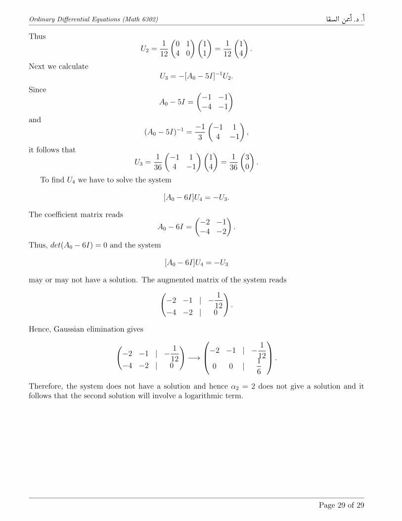
Thus

U2 =1

12

(0 14 0

)(11

)=

1

12

(14

).

Next we calculateU3 = −[A0 − 5I]−1U2.

Since

A0 − 5I =

(−1 −1−4 −1

)and

(A0 − 5I)−1 =−1

3

(−1 14 −1

),

it follows that

U3 =1

36

(−1 14 −1

)(14

)=

1

36

(30

).

To find U4 we have to solve the system

[A0 − 6I]U4 = −U3.

The coefficient matrix reads

A0 − 6I =

(−2 −1−4 −2

).

Thus, det(A0 − 6I) = 0 and the system

[A0 − 6I]U4 = −U3

may or may not have a solution. The augmented matrix of the system reads(−2 −1 | − 1

12−4 −2 | 0

).

Hence, Gaussian elimination gives

(−2 −1 | − 1

12−4 −2 | 0

)−→

−2 −1 | − 1

12

0 0 | 1

6

.

Therefore, the system does not have a solution and hence α2 = 2 does not give a solution and itfollows that the second solution will involve a logarithmic term.

of 29

Chapter 4 Series Solutions and Frobenius Method

Documents

Transcript of Chapter 4 Series Solutions and Frobenius Method