arX

iv:n

lin/0

1050

47v1

[nl

in.C

D]

21

May

200

1

Resonances of the Frobenius-Perron Operator for a Hamiltonian Map with a Mixed

Phase Space

Joachim Weber1,2, Fritz Haake1, Petr A. Braun1,3, Christopher Manderfeld1, and Petr Seba4

1 Fachbereich Physik, Universitat-GH Essen, 45117 Essen, Germany

2 Department of Physics of Complex Systems, Weizmann Institute of Science, Rehovot 76100, Israel

3 Institute of Physics, Saint-Petersburg University, Saint-Petersburg 198504, Russia

4 Institute of Physics, Czech Academy of Sciences, Prague, Czech Republic

(Date: January 3, 2014)

Resonances of the (Frobenius-Perron) evolution operator P for phase-space densities have recentlyattracted considerable attention, in the context of interrelations between classical and quantumdynamics. We determine these resonances as well as eigenvalues of P for Hamiltonian systems witha mixed phase space, by truncating P to finite size in a Hilbert space of phase-space functionsand then diagonalizing. The corresponding eigenfunctions are localized on unstable manifolds ofhyperbolic periodic orbits for resonances and on islands of regular motion for eigenvalues. Usinginformation drawn from the eigenfunctions we reproduce the resonances found by diagonalizationthrough a variant of the cycle expansion of periodic-orbit theory and as rates of correlation decay.

I. INTRODUCTION

Chaotic behavior in classical Hamiltonian systems manifests itself in an infinite hierarchy of phase-space structuresand instability of trajectories with respect to small changes in their initial condition. If resolution in phase space isrestricted, e.g. due to finite precision of measurements, phase-space trajectories can be followed only approximately.Every finite-resolution initial condition actually stands for an entire ensemble of trajectories with possibly very differentlong-time behaviors. That fact suggests a probabilistic approach to the dynamics, in which a phase-space density andits propagator P , the so called Frobenius-Perron operator, are studied.

Because of Liouville’s theorem P can be represented by an infinite unitary matrix in a Hilbert space of phase-spacefunctions. The spectrum of P thus lies on the unit circle in the complex plane. Discrete eigenvalues represent regulardynamics, while chaos entails a continuous spectrum, and along with the latter resonances of P may occur thatcharacterize effectively irreversible behavior [1,2]. Apart from their role as decay rates, Frobenius-Perron resonanceshave been found to link classical with quantum dynamics because they could as well be identified from quantumsystems [3,4]. Furthermore, they have been predicted to carry information on the system-specific corrections touniversality of quantum fluctuations [5,6].

To identify resonances, mathematically defined as singularities of the resolvent of P in some higher Riemanniansheet, it is necessary to analytically continue the resolvent across the continuous spectrum of P from the outside tothe inside of the unit circle [7–9]. This becomes increasingly difficult as the dynamics gains complexity. Especiallyfor the large class of systems with a mixed phase space an effective approximation scheme is needed that is free ofrestrictions of previous investigations [10,11], such as hyperbolicity, one-dimensional (quasi-) phase space, or isolationof the phase-space regions causing intermittency.

In the following we present such a scheme and illustrate it for a prototypical dynamical system with a mixed phasespace, a periodically kicked top. We represent P in a Hilbert space of phase-space functions as an infinite unitarymatrix and subsequently truncate it to a finite N -dimensional matrix P(N), with resolution in phase space as thetruncation criterion. We thus generate a nonunitary approximation to the unitary P that becomes exact as N → ∞.Looking at the spectra of P(N) with increasing N , we find some eigenvalues persisting in their positions, eitheralmost on the unit circle or well inside, and we focus on these “frozen” eigenvalues. While frozen (near)unimodulareigenvalues of P(N) turn into unimodular eigenvalues of P as N → ∞, the nonunimodular frozen eigenvalues arenot part of the spectrum of P in that limit. We will argue that at finite but large N they rather indicate thepositions of resonances of P . Accordingly, the eigenfunctions of P(N) are of very different nature for these twocases. We find eigenfunctions to unimodular eigenvalues localized and approximately constant on islands of regularmotion in phase space that are bounded by invariant tori. In contrast, eigenfunctions to nonunimodular eigenvaluesof P(N) are localized near unstable manifolds of hyperbolic periodic orbits. Just as nonunimodular eigenvalues arenot in the spectrum of the Hilbert-space operator P , the eigenfunctions are no Hilbert-space functions in the limitof infinite resolution. A comparison of the eigenfunctions of P(N) for different values of N and furthermore with theeigenfunctions of the truncated inverse operator P−1(N) illustrates why they lie outside the Hilbert space. The stronglocalization of these (resonance-)eigenfunctions at finite N allows us to identify the relatively few groups of periodic

1

orbits associated with a particular resonance up to a certain length. From only these orbits we recover resonances viaa variant of the so-called cycle expansion of periodic-orbit theory that works even in the case of a mixed phase space.To verify that frozen eigenvalues have indeed the physical interpretation of resonances, we conclude with a numericalexperiment in which the decay of a two-point correlation function is observed. In order to find a certain resonanceresponsible for correlation decay, the initial phase-space density is chosen localized in the phase-space region wherethe resonance-eigenfunction has large amplitudes.

A short account of the results to be discussed here has been published recently [12].

II. LIOUVILLE DYNAMICS ON THE SPHERE

As a prototypical Hamiltonian system with a phase space displaying a mix of chaotic and regular behavior weconsider a periodically kicked angular momentum vector

(Jx, Jy, Jz) = (j sin θ cosϕ, j sin θ sinϕ, j cos θ) (1)

of conserved length j, also known as the kicked top [13]. Such a system has one degree of freedom, and its phasespace is a sphere. A phase-space point X ≡ (p, q) may be characterized by an “azimutal” angle ϕ as the coordinateq and the cosine of a “polar” angle θ as the conjugate momentum p. The dynamics is specified as a stroboscopicarea preserving map, X ′ = M(X). We chose M to consist of rotations Rz(βz), Ry(βy) about the y- and z-axes and a“torsion”, i.e. a nonlinear rotation Tz(τ) = Rz(τ cos θ) about the z-axis which changes ϕ by τ cos θ,

M = Tz(τ)Rz(βz)Ry(βy) . (2)

In the sequel we keep βz = βy = 1 fixed and vary the torsion constant τ to generate a phase space which is integrablefor τ = 0 and increasingly dominated by chaos as τ grows. We focus on τ = 2.1 as a moderately chaotic case andτ = 10.2 as strongly chaotic (see figures 1a,b), where elliptic islands have become so small that they are difficult todetect.

In the Liouville picture the time evolution of a phase-space density ρ is governed by Liouville’s equation,

∂tρ = Lρ = H, ρ , (3)

where the Liouville operator L, the Poisson bracket with the Hamiltonian H , appears as generator. For our rotationsand torsion we separately take H = βyJy, H = βzJz, and H = (τ/2)J2

z . Denoting the respective Liouvillians by LRy,

LRz, and LTz

we imagine Liouville’s equation for each of them integrated over a unit time span. The product of theresulting three propagators yields our Frobenius-Perron operator P = exp(LTz

) exp(LRz) exp(LRy

). The action of Pon the phase-space density ρ(q, p) can be represented in terms of the ”Hamilton-picture” map M as

ρn+1(X) = P ρn(X) = eLTz eLRz eLRy ρn(X)

=

∫

dX ′ δ(X −M(X ′)) ρn(X ′) . (4)

Since the map M is invertible and area preserving, det ∂M(X)/∂X = 1, the integral simplifies to

Pρ(X) = ρ[

M−1(X)]

. (5)

While a phase-space density is usually considered as L1-integrable it can be assumed to belong to a Hilbert spaceof L2-functions as well. The additional structure of the Hilbert space can be exploited to represent P by an infiniteunitary matrix, the unitarity (Pρ1,Pρ2) = (ρ1, ρ2) following from (5) and area preservation in the map M . The basisfunctions may be chosen as ordered with respect to phase-space resolution. This allows us to eventually truncate Pto finite size and still retain the propagator intact for functions on large phase-space scales.

On the unit sphere the spherical harmonics Ylm(ϕ, cos θ) with l = 0, 1, 2, . . . and integer |m| ≤ l form a suitablebasis. Phase-space resolution is characterized by the index l: using all Ylm with 0 ≤ l ≤ lmax phase-space structuresof area ∝ 1/l2max can be resolved, and the number of these basis functions is N = (lmax + 1)2.

To check on the resolution achievable by spherical harmonics consider a Gaussian G(ϕ, θ) =exp (−i(ϕ− ϕ0)

2/∆ϕ2 − i(θ − θ0)2/∆θ2) with the angular widths ∆ϕ,∆θ and the effective area ∼ ∆ϕ∆θ. To

represent it by a linear combination of spherical harmonics we need only the Ylm with |m| ≤ m0 ∼ 2π/∆ϕ andl ≤ 2π/∆ϕ + π/∆θ; all other spherical harmonics have negligible scalar product with G(ϕ, θ). Indeed, the effective

2

“wavelengths” of Ylm in ϕ and θ are, respectively, 2π/|m| and π/(l − |m|), the latter given by the number (l − |m|)of zeros of the Legendre function Plm in the interval 0 < θ < π; once these wavelengths become smaller then therespective widths ∆ϕ,∆θ of the Gaussian the overlap of G and Ylm is negligible. Inverting that statement we maysay that a basis set of spherical harmonics cut off at a certain lmax is suitable for representing objects on the unitsphere with the angular sizes ∼ lmax and area ∼ l2max.

To obtain the matrix elements

Plm,l′m′ =

∫ 1

−1

d cos θ

∫ 2π

0

dϕ Y ∗lm(ϕ, cos θ)Yl′m′

[

M−1(ϕ, cos θ)]

(6)

for the mixed dynamics it is convenient to first determine the Frobenius-Perron matrices for the two rotationsexp(LRz

), exp(LRy) and the torsion exp(LTz

), all of which are by themselves integrable and free of chaos. Defer-ring the derivation to Appendix A we here just note the three matrices. The Frobenius-Perron matrix of the z-rotation is diagonal,

(

exp(LRz))

lm,l′m′

= δll′δmm′ exp(−imβz) . (7)

For the y-rotation, (exp(LRy))lm,l′m′ is blockdiagonal in l with the blocks well known from quantum mechanics as

Wigner’s d-matrices,

(

exp(LRy))

lm,l′m′

= δll′dlmm′(βy) . (8)

For the z-torsion the Frobenius-Perron matrix elements are given by finite sums over products of spherical Besselfunctions jl(x) and Clebsch-Gordan coefficients,

(

exp(LTz))

lm,l′m′

= δm,m′(−1)m√

(2l + 1)(2l′ + 1)

×l+l′∑

l′′=|l−l′|

(−i)l′′ jl′′ (mτ) Cl l′ l′′

0 0 0 Cl l′ l′′

−m m 0 . (9)

Finally, for the mixed dynamics P is the product of the three above matrices. Due to the Kronecker deltas involved,each element of P is just the product of three matrix elements, one each for the rotations and the torsion. Obviously,P is a full matrix coupling all phase-space scales, as it is to be expected for chaotic dynamics. We furthermore remarkthat with respect to the real basis

yl0 = Yl0

y+lm =

1√2(Ylm + Y ∗

lm) , (10)

y−lm =1√2i

(Ylm − Y ∗lm)

the matrix P is also real , since real phase-space densities cannot become complex under time evolution. As aconsequence, all eigenvalues of P(N) are either real or come in complex conjugate pairs.

III. RESONANCES AND EIGENVALUES AT FINITE PHASE-SPACE RESOLUTION

To study resonances and (discrete) eigenvalues of P we investigate the finite-size approximants P(N) for differentvalues of N , i.e. different resolutions in phase space. In the low-resolution subspace spanned by the first N basisfunctions P(N) replaces P identically, but it completely rejects fine phase-space structures that cannot be expandedin terms of these N functions.

The truncation of P to finite size breaks unitarity. Therefore, P(N) may not only have unimodular eigenvaluesbut also eigenvalues located inside the unit circle. Furthermore, the spectrum of P(N) is purely discrete. The N -dependence of the eigenvalues of P(N) yields information on the spectral properties of P . Upon diagonalizing P(N)

and increasing N we find the “newly born” eigenvalues close to the origin while the “older” ones move about in thecomplex plane. “Very old” ones eventually settle for good. If the classical dynamics is integrable (τ = 0 or βy = 0),

3

the asymptotic large-N loci are back to the unit circle, where the full P has its discrete eigenvalues. The situationis different for the mixed phase space: while some eigenvalues of P(N) “freeze” with unit moduli, others come torest inside the unit circle as N → ∞. These eigenvalues reflect resonances of P in a higher Riemannian sheet of thecomplex plane. We see this phenomenon as analogous to the spectral concentration in perturbation theory [14,7,15]:a perturbation series for an operator with continuous spectrum does not converge but produces, with increasing order,a sequence of points concentrated in the neighborhood of the respective resonance.

An additional intuitive argument for the persistence of non-unimodular eigenvalues as N → ∞ for nonintegrabledynamics is the following: in contrast to regular motion, chaos comes with a hierarchy of phase-space structures whichextends without end to ever finer scales. Probability that is propagated from large to fine scales mostly does notreturn. This effectively dissipative character of the conservative dynamics is accounted for as true dissipation by thetruncated propagator and its nonunimodular eigenvalues, but the difference between effective and true dissipation isirrelevant for low resolution. Moreover, a frozen nonunimodular eigenvalue is to be understood as a scale-independentdissipation rate, in tune with the expected selfsimilarity in phase space.

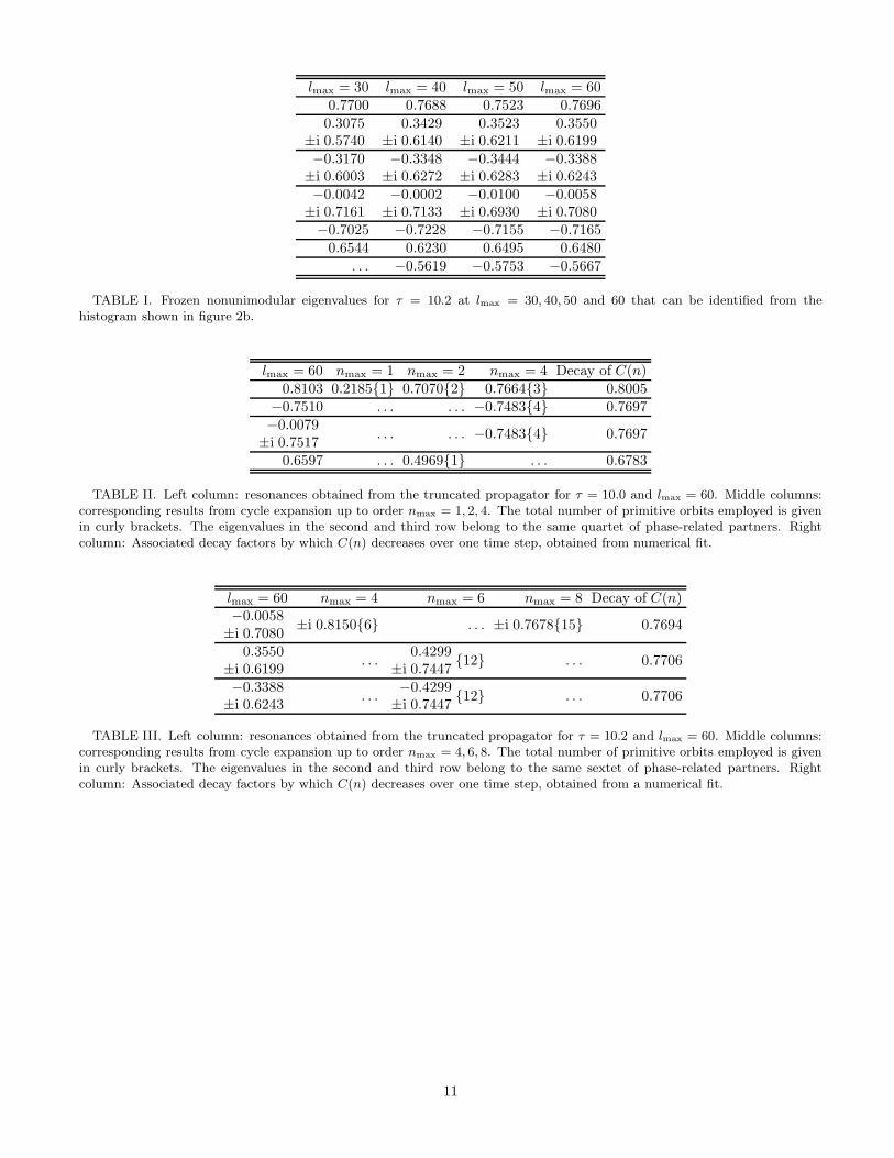
The freezing of non-unimodular eigenvalues is illustrated for two kicked tops, one with weakly chaotic (τ = 2.1)and one with strongly chaotic character (τ = 10.2). Figures 1a and 1b show the respective phase-space portraits.While for τ = 2.1 large islands of regular motion still exist, for τ = 10.2 regular islands have become so small thatthey are difficult to detect and impossible to resolve with lmax = 70. Figures 2a and 2b show grey-shade codedhistograms in the complex plane for the number of eigenvalues with moduli larger than 0.2 of all matrices withlmax = 40, 41, 42, . . .70. Eigenvalues with moduli smaller than 0.2 are rejected because they have not settled yetand their density near the origin is so high that they would spoil the histogram. Large amplitudes (black) in thehistograms indicate the positions of frozen eigenvalues. While for τ = 2.1 a large number of frozen eigenvalues is foundclose to the unit circle, in the case τ = 10.2, where no regular islands can be resolved, the only unimodular eigenvalueis the one at unity which pertains to the stationary uniform eigenfunction Y00; all other frozen eigenvalues lie wellinside the unit circle and indicate resonance positions. Table I lists some of these frozen nonunimodular eigenvaluesat resolutions lmax = 30, 40, 50 and 60.

At first sight the two cases presented above may appear to correspond to quite different types of dynamics, butactually this is only a matter of resolution. As resolution is further increased in the strongly chaotic case (τ = 10.2),elliptic islands will be resolved at some stage. Correspondingly, eigenvalues of P(N) will emerge which freeze on theunit circle. Also new nonunimodular frozen eigenvalues may appear, possibly even ones larger in modulus than thefrozen eigenvalues found at lower resolution.

IV. EIGENFUNCTIONS AND RESONANCE-EIGENFUNCTIONS AT FINITE PHASE-SPACE

RESOLUTION

An investigation of the eigenfunctions of P(N) reveals more about the nature of the frozen eigenvalues. Eigenvaluesfreezing with unit moduli have eigenfunctions located on elliptic islands of regular motion surrounding elliptic periodicorbits in phase space. Such islands are bounded by invariant tori which form impenetrable barriers in phase space.Thus if χp,n is a characteristic function constant on an island around the nth point of an p-periodic orbit and zerooutside with χp,n+1 = Pχp,n and χp,1 = Pχp,p, then

fp =

p∑

n=1

χp,n (11)

is an eigenfunction of P with eigenvalue unity. Moreover, linear combinations of such functions are eigenfunctions aswell. Figures 3a,b show two eigenfunctions of P(N) with eigenvalues 0.999976 and 0.999974 almost at unity for thekicked top with τ = 2.1 and lmax = 60. Amplitudes of the functions are large in dark shaded areas of phase space.The elliptic islands supporting the eigenfunctions can easily be identified in the phase-space portrait in figure 1a.

For p > 1 we furthermore expect and find the pth roots of unity as eigenvalues as well with eigenfunctions thathave constant moduli on elliptic islands and are invariant under Pp,

fp,m =

p∑

n=1

ei2πmn/pχp,n , with m = 1, . . . , p . (12)

Superpositions of two such fp,m, fp′,m′ are also eigenfunctions if m/p = m′/p′, i.e. if all periods p′ involved aremultiples of p; the possible phases are dictated by the shortest period p.

4

Once freezing has been observed for eigenvalues with moduli smaller than unity their eigenfunctions have approachedtheir final shape on the resolved phase-space scales. In contrast to the eigenfunctions with unimodular eigenvaluesthese eigenfunctions are localized around unstable manifolds of hyperbolic periodic orbits, ones with low periods atfirst since these are easiest to resolve. [Typically, for every period several neighbouring orbits of approximately equalinstability can be identified in an eigenfunction, their number being the larger the more extended the eigenfunction.]Figure 4 shows moduli of eigenfunctions for some of the nonunimodular eigenvalues listed in table I at resolutionlmax = 60. Particularly in figures 4b,c the localization on orbits of length six and four respectively is obvious.With growing lmax more orbits of higher periods appear in the eigenfunction. Their supports gain complexity, incorrespondence with the infinitely convoluted shape of the unstable manifolds. Just as for the eigenvalues there is nostrict convergence of the eigenfunctions. Since no finite approximation P(N) accounts for arbitrarily fine structuresone encounters the aforementioned loss of probability from resolved to unresolved scales. Not even in the limit N → ∞can the unitarity of P be restored: rather, in tune with a continuous spectrum of P , the eigenfunctions tend to singularobjects outside the Hilbert space. This becomes even more obvious in a comparison of eigenfunctions of P(N) witheigenfunctions of the truncated inverse propagator P−1(N). Both matrices have the same frozen eigenvalues, but onlyfor the unimodular ones eigenfunctions of P(N) and P−1(N) to the same eigenvalue have (roughly) the same support,as it is expected for unitary dynamics: the elliptic islands that support the eigenfunctions are invariant under timereversal. For nonunimodular frozen eigenvalues eigenfunctions of P(N) and P−1(N) have distinct supports. Whileunstable periodic orbits are traversed in the opposite direction but remain the same under time reversal, stable andunstable manifolds are interchanged. Thus the eigenfunctions of P−1(N) are localized near the same periodic orbitsbut around the stable manifolds of the forward-dynamics. In particular the eigenfunctions do not converge to thesame limit as N → ∞. Needless to say this again reflects the effective irreversibility of the chaotic Hamiltoniandynamics. Figures 5 and 6 illustrate the aforesaid. The eigenfunction in figure 5a at resolution lmax = 30 correspondsto the same frozen eigenvalue as the eigenfunction in figure 5b at resolution lmax = 60. While coarse structures arethe same in both eigenfunctions, more fine structures appear at the higher resolution. Figure 5c shows, again for thesame eigenvalue, the eigenfunction of P−1(N) at lmax = 60. In contrast to figure 5b localization is now on the stablemanifolds of the same periodic orbits of the foreward dynamics. These periodic orbits as well as their unstable andstable manifolds are shown in figure 6.

Just like the unimodular eigenvalues, frozen eigenvalues inside the unit circle come in p-families, i.e. with phasescorresponding to the pth roots of unity, determined by the length p of the shortest periodic orbit present in aneigenfunction. Now the above argument must be modified in the following way: assume an eigenfunction f is mostlyconcentrated around a shortest unstable orbit with period p as well as a longer one with period p′. Denote by ψp,n

again a “characteristic function”, now constant near the n-th point of the period−p orbit, n = 1 . . . p, and zeroelsewhere. The truncated Frobenius-Perron operator P(N) maps ψp,n into P(N)ψp,n = rpψp,n+1 with the real positivefactor rp smaller than unity accounting for losses, in particular to unresolved scales. As previously, independent linearcombinations of the ψp,n can be formed as

fp,m =

p∑

n=1

ei2πmn/pψp,n with m = 1 . . . p . (13)

Now consider a sum of two such functions, g = fp,m + fp′,m′ , and apply P(N). For g to qualify as an approximateeigenfunction we must obviously have rp ≈ rp′ , i.e. the two periodic orbits must be similarly unstable, and m/p =m′/p′. But then indeed P(N)g ≈ rpe

i2πm/pg and [P(N)]pg ≈ rppg, and the phase is dictated by the shortest orbit. Since

orbits of low period are most likely to be resolved first, usually the first frozen eigenvalues found from diagonalizingP(N) have phases corresponding to small numbers p. Since nonunimodular eigenvalues with phases according top = 1, 2, 4 have already been presented in [12], in this paper we intentionally chose τ = 10.2, a case for whicheigenvalues with other phases happen to be more easily detected. In figure 2b and table I complex eigenvalues withphases near the sixth roots of unity are clearly visible.

V. PERIODIC-ORBIT EXPANSION OF THE SPECTRAL DETERMINANT

Since the unstable periodic orbits that are linked to a nonunimodular eigenvalue can be identified quite easily fromthe eigenfunction of P(N), one is tempted to adopt a cycle expansion to calculate decay rates from periodic orbits.

For purely hyperbolic systems, cycle expansions of the spectral determinant, i.e. the characteristic polynomial ofthe Frobenius-Perron operator

5

d(z) = det(1 − zP) = exp tr ln(1 − zP) (14)

are known to allow for the calculation of resonances with high accuracy [16,17]. The spectral determinant is expressedin terms of the traces of the Frobenius-Perron operator tr Pn as

d(z) =

∞∏

n=1

exp

(

−zn

ntr Pn

)

(15)

and subsequently expanded as a finite polynomial up to some order nmax. Only the first nmax traces are required forthe calculation of this polynomial, and only periodic orbits with primitive periods up to nmax contribute to it.

The traces

tr Pn =

∫

dX δ(X −Mn(X)) (16)

are calculated as sums over hyperbolic periodic orbits of length n as

tr Pn =∑

X=MnX

1

| det(1 − Ξn)| (17)

where the matrix Ξn = ∂Mn(X)/∂X is the linearized version of the map Mn evaluated at any of the points of aperiod−n orbit. If n is the r-fold of a primitive period p, the matrix Ξn can as well be written as Ξn = Ξr

p, and thespectral determinant as a product of contributions from all primitive orbits k,

d(z) =∏

k

exp

[

−∞∑

r=1

1

r

zpkr

det(1 − Ξrpk

)

]

. (18)

The zeros zi of the polynomial which are insensitive against an increase of nmax are inverses of resonances.For the ordinary cycle expansion of a spectral determinant just sketched to converge, all periodic orbits must be

hyperbolic and sufficiently unstable [1,16,17]. These conditions are not met for a mixed phase space, not only becauseof the presence of elliptic orbits but also because of very weakly unstable orbits with high periods. We can circumventsuch limitations by considering only one ergodic region in phase space at a time, bar contributions from elliptic orbits,and impose a stability bound by including only the relatively few, about equally unstable hyperbolic orbits ki

identified in an eigenfunction of P(N). We surmize that the spectral determinant factors as

d(z) =

∞∏

i=1

di(z) , (19)

with one factor di for the family ki of periodic orbits showing up in the ith eigenfunction. Each such factor di(z) isthen calculated separately with the above expressions. Obviously this variant of the cycle expansion reproduces thephases of the resonances exactly since these are again directly determined by lengths of orbits: if p is the smallestperiod used in di(z), the polynomial can as well be written as a polynomial in zp thus allowing the zeros to have thephases of the pth roots of unity. Needless to say, the notorious proliferation of periodic orbits with growing lengthcauses more and more difficulties for the cycle expansion for p-families of resonances with increasing p.

We first turn to the top with τ = 10. Here, unstable orbits with periods 1,2, and 4 and the corresponding p-familiesof resonances are easily detected. In Table II frozen eigenvalues found at the resolution lmax = 60 are listed in the firstcolumn. The columns to the right show the corresponding results of the cycle expansion up to order nmax = 1, 2, 4.The total number of orbits used in each case is given in curly brackets. For instance, our cycle expansion of theresonance 0.81 involves three orbits of lengths 1, 2 and 4. The resonance −0.7510 as well as its phase-related partners−0.0079 ± i0.7517 can be approximately reproduced using four orbits of length 4. For the real positive eigenvalue0.7470 (not listed in table II) completing this quartet of eigenvalues the eigenfunction is also localized in other regionsof phase space and thus further orbits with periods different from p = 4 would have to be included in the cycleexpansion. The first repetition of the single period-2 orbit contributing to the resonance 0.6597 in table II gives analmost diverging contribution to the spectral determinant, thus hindering its expansion to a higher order.

The top with τ = 10.2 offers itself for a study of complex frozen eigenvalues with phases near the fourth andsixth roots of unity. Even though these two groups of eigenvalues are almost equal in modulus, the correspondingeigenfunctions are localized in different regions of phase space, and therefore the two examples turn out independent

6

(see figures 4b,c). The reason why we leave aside the eigenvalues on the real axis is that their eigenfunctions showlocalization on many orbits of different, higher periods which cannot all be identified (see figures 4a,d). For theresonances −0.0058± i0.7080 the spectral determinant of order nmax = 4, calculated from six periodic orbits of length4, yields ±i0.8150. In the next higher order nmax = 8 another 9 orbits of primitive length 8 must be taken intoaccount with the resulting approximants ±i0.7678. For the resonances 0.3550 ± i0.6199 and −0.3388 ± i0.6243 withphases near the sixth roots of unity 12 orbits of primitive length 6 contribute to the spectral determinant in lowestorder. These orbits are shown in figure 6a. In lowest order the resulting six approximants of modulus 0.8599 stilldiffer by about 20% from the respective moduli 0.7144 and 0.7103. These results are compiled in Table III.

VI. RESONANCES VERSUS CORRELATION DECAY

To check on the physical meaning of frozen eigenvalues with moduli smaller than unity as Frobenius-Perron reso-nances we propose to compare their moduli with rates of correlation decay. In a numerical experiment we investigatethe decay of the correlator

C(n) =〈ρ(n)ρ(0)〉 − 〈ρ(∞)ρ(0)〉〈ρ(0)2〉 − 〈ρ(∞)ρ(0)〉 . (20)

The initial densities ρ(0) are chosen as characteristic functions on a grid of 2000 × 2000 cells in phase space. Eachcell is represented by its central point (q, p)c, and its temporal successor after one time step is the cell containingM((q, p)c). After n iterations we obtain ρ(n). From the phase-space average 〈ρ(n)ρ(0)〉 we subtract the correlationsremaining at n = ∞ due to the compactness of the phase space, and subsequently normalize.

Depending on the choice of ρ(0) different long-time decays are observable. We choose ρ(0) as covering the regionswhere the hyperbolic orbits relevant for a given resonance are situated. The long-time decay turns out insensitiveto the exact choice of ρ(0), provided ρ(0) does not extend to phase-space regions supporting different eigenfunctionswith frozen eigenvalues of larger moduli. Since ρ(0) is real and positive, and positivity is preserved under the timeevolution, we find positive real decay factors C(n+1)/C(n). Indeed, after two or three time steps these decay factorsare in rather good agrement with the modulus of the corresponding nonunimodular eigenvalue as well as with theresult of our cycle expansion. Tables II and III list the decay factors we obtained from a numerical fit of C(n) fromn = 2 to n = 18, together with the moduli of the respective resonances. Figure 7 shows the decay of C(n) (dots), withρ(0) chosen according to the eigenfunction shown in figure 4b. The numerical fit (line) yields a decay factor 0.7706,to be compared with 0.7103 as the modulus of the eigenvalue.

VII. CONCLUSIONS

In conclusion, we have presented a method to determine Frobenius-Perron resonances and eigenvalues which isapplicable to systems with a mixed phase space. Resonances as well as eigenvalues are identified as frozen eigenvaluesof a truncated propagator matrix P(N) in a Hilbert space of phase-space functions. The corresponding eigenfunctionsof P(N) are strongly localized on the associated phase-space structures, elliptic islands for eigenvalues and unstablemanifolds of hyperbolic periodic orbits for resonances. The expected characteristics of the resonance eigenfunctions,an infinite hierarchy of structures and the distinct supports of foreward and backward time evolution, are clearlyvisible. The resonances obtained can be reproduced by a variant of the cycle expansion in which only the orbitsthat are identified in the eigenfunctions are taken into account. Finally, the correlation decay within a phase-spaceregion that an eigenfunction is localized in is well predicted by the corresponding resonance. The cycle expansion aswell as the observation of correlation decay may be used to check the accuracy of the resonances obtained as frozeneigenvalues. An accurate knowledge of the relevant resonances of mixed dynamics at a certain phase-space resolutionis a desirable piece of information for many further investigations such as the role of classical resonances in quantumdynamics.

We are grateful to Shmuel Fishman for discussions initiating as well as accompanying this work. Support by theSonderforschungsbereich “Unordnung und große Fluktuationen” and the Minerva foundation is thankfully acknowl-edged.

7

VIII. APPENDIX A: MATRIX ELEMENTS OF THE FROBENIUS-PERRON OPERATOR

We here derive the matrix elements (6) of the Frobenius-Perron operator P . It is convenient to use the representationof Ylm in terms of associated Legendre Polynomials Pm

l (x) [19],

Ylm(q, p) = (−1)m

[

2l+ 1

4π

(l −m)!

(l +m)!

]1

2

Pml (p) eimq , (21)

For rotations Ry, Rz and torsion Tz on the unit sphere the explicit forms for M read

Ry(βy) :

(

q

p

)

7−→(arg

(

√

1 − p2 (cosβy cos q + i sin q) + p sinβy

)

p cosβy −√

1 − p2 sinβy cos q

)

Rz(βz) :

(

q

p

)

7−→(

q + βz

p

)

(22)

Tz(τ) :

(

q

p

)

7−→(

q + τp

p

)

.

The above immediately implies the intuitive result for the z-rotation

Ylm

(

R−1z (q, p)

)

= e−imβzYlm(q, p) . (23)

Due to the orthonormality of the spherical harmonics we then find the Frobenius-Perron operator represented by thediagonal matrix

exp(LRz)l1m1,l2m2

= δl1l2 δm1m2e−im2βz . (24)

Obviously and intuitively, exp(LRz) is identical to the quantum mechanical (h = 1) rotation matrix

〈l1m1| exp(−iβzLz)|l2m2〉 involving the Lz-component of the angular momentum operator ~L = (Lx, Ly, Lz)T and

the eigenbasis Ylm = |lm〉 with ~L2|lm〉 = l(l + 1)|lm〉 and Lz|lm〉 = m|lm〉. Since this formal identity holds for thez-rotation it must also hold for the y-rotation. Thus for exp(LRy

) we must take the representation of the quantumoperator exp(−iβyLy), well known as Wigner’s d-matrix,

exp(LRy)l1m1,l2m2

= 〈l1m1| exp(−iβyLy)|l2m2〉 = δl1l2 dl1m1m2

(βy) , (25)

which can be obtained from recursion relations [18]. This matrix is still diagonal in l1, l2. In fact, the Frobenius-Perronmatrix for any rotation is diagonal in that pair of indices. An immeditate implication is that pure rotations do notcouple the subspace of Ylm with l ≤ lmax to its complement. For the integrable dynamics of rotation no probabilityis dissipated from the subspace and the spectrum of P(N) lies exactly on the unit circle.

For the z-torsion we make the replacement

Ylm(T−1z (q, p)) = e−iτmp Ylm(q, p) (26)

in the phase-space integral (6) and then use the expansion [20]

e−ik cos θ =

∞∑

l=0

(−i)l√

4π(2l + 1) jl(k) Yl0(ϕ, cos θ) , (27)

which involves the spherical Bessel function jl(k). The parity Y ∗l1m1

= (−1)m1Yl1,−m1helps us on to

exp(LTz)l1m1,l2m2

= (−1)m1

∞∑

l=0

(−i)l√

4π(2l+ 1)jl(m1τ)

∫

Ω

dq dp Yl0 Yl1,−m1Yl2m2

. (28)

We here meet Gaunt’s integral [21] over three spherical harmonics which can be written in terms of two Clebsch-Gordancoefficients,

∫

Ω

dq dp Y ∗lm Yl1m1

Yl2m2=

[

(2l1 + 1)(2l2 + 1)

4π(2l + 1)

]1

2

Cl1 l2 l0 0 0 Cl1 l2 l

m1m2m . (29)

8

Finally, using the following properties of Clebsch-Gordan coefficients,

Cl1 l2 lm1m2m = 0 if l /∈ (l1 + l2), (l1 + l2) − 1, . . . , |l1 − l2| ,

Cl1 l2 lm1m2m = 0 if m1 +m2 6= m, (30)

Cl1 l2 l0 0 0 = 0 if l1 + l2 + l odd

the infinite sum in (28) can be reduced to a finite one,

exp(LTz)l1m1,l2m2

= δm1m2(−1)m1

√

(2l1 + 1)(2l2 + 1)

l1+l2∑

l=|l1−l2|

(−i)l jl(m1τ) Cl1 l2 l0 0 0 Cl1 l2 l

−m1m20. (31)

It is worth noting that due to the properties (30) the matrix elements (31) are real if l1+ l2 is even or purely imaginaryif l1 + l2 is odd. Furthermore they are symmetric with respect to l1 and l2.

IX. APPENDIX B: RECURSION RELATION FOR THE TORSION MATRIX ELEMENTS

A recursion relation similar to the recursion relation used to calculate Wigner’s d-matrix can be derived for thetorsion matrix elements. For simplicity we consider the integral

tz(l′, l,m) =

∫ 1

−1

du Pml′ (u) eiτmu Pm

l (u) (32)

which is related to the torsion matrix elements by

exp(LTz)l′mlm =

1

2

[

(2l′ + 1)(l′ −m)!

(l′ +m)!

(2l + 1)(l −m)!

(l +m)!

]1

2

tz(l′, l,m) . (33)

The associated Legendre polynomials obey the differential equation

DPml (u) ≡

[

(1 − u2)d2

du2− 2u

d

du+ l(l+ 1) − m2

1 − u2

]

Pml (u) = 0 . (34)

This suggests to draw a recursion relation from

∫ 1

−1

du [DPml′ (u)] Pm

l (u) eiτmu = 0 . (35)

In the case m 6= 0 integration by parts leads to

∫ 1

−1

duPml′ eiτmu

[

(2iτm)(

(1 − u2)d

duPm

l − u Pml

)

+ (36)

(

l′(l′ + 1) − l(l + 1) − (1 − u2) τ2m2)

Pml

]

= 0 .

Now with the help of the identity

(1 − u2)d

duPm

l = −luPml + (l +m)Pm

l−1 (37)

the derivative in (36) can be eliminated and we arrive at the five-step recursion relation

tz(l′, l + 2,m) =

1

τ2m2

(2l + 1)(2l+ 3)

(l −m+ 1)(l −m+ 2)

[

2iτm(l + 1)(l −m+ 1)

2l+ 1tz(l

′, l + 1,m)

−(

l′(l′ + 1) − l(l+ 1) − 2τ2m2 l(l + 1) +m2 − 1

4l(l+ 1) − 3

)

tz(l′, l,m) (38)

−2iτml(l +m)

2l + 1tz(l

′, l − 1,m) − τ2m2 (l +m)(l +m− 1)

(2l + 1)(2l− 1)tz(l

′, l − 2,m)

]

.

9

For constant indices l′ and m 6= 0 this links matrix elements with five successive values of the index l. Just likethe torsion matrix elements for these indices the terms in the recursion relation have alternately real and imaginaryvalues. Even though the recursion relation involves five matrix elements, only two integrals have to be done initially.These are the nonvanishing integrals tz(l

′, |m|,m) and tz(l′, |m| + 1,m) for the smallest values of l. Together with

tz(l′, |m| − 1,m) = 0 and tz(l

′, |m| − 2,m) = 0 they can be used to start the recursion.For m = 0 the recursion formula does not apply, but the integral

tz(l′, l, 0) =

2

2l+ 1δll′ (39)

is trivial in this case.

[1] D. Ruelle, Phys. Rev. Lett. 56, 405 (1986); D. Ruelle, J. Stat. Phys. 44, 281 (1986).[2] M. Pollicott, Invent. Math. 81, 415 (1985)[3] F. Haake, C. Manderfeld, J. Weber, and P. A. Braun, in preparation[4] K.Pance, W. Lu, S. Sridhar, Phys. Rev. Lett. 85, 2737 (2000)[5] A. V. Andreev and B. L. Altshuler, Phys. Rev. Lett. 75, 902 (1995); O. Agam, B. L. Altshuler, and A. V. Andreev, Phys.

Rev. Lett. 75, 4389 (1995); A. V. Andreev,O. Agam, B. D. Simons, and B. L. Altshuler, Phys. Rev. Lett. 76, 3947 (1996);A. V. Andreev, B. D. Simons, O. Agam, and B. L. Altshuler, Nuclear Physics B, 482, 536 (1996).

[6] M. R. Zirnbauer in: I.V. Lerner, J.P. Keating, and D.E. Khmelnitskii (eds.), Supersymmetry and Trace Formulae: Chaos

and Disorder (Kluwer Academic, New York, 1999)[7] M. Reed and B. Simon, Methods of Modern Mathematical Physics IV: Analysis of Operators (Academic Press, New York,

1978).[8] S. Fishman in: I.V. Lerner, J.P. Keating, and D.E. Khmelnitskii (eds.), Supersymmetry and Trace Formulae: Chaos and

Disorder (Kluwer Academic, New York, 1999)[9] M. Khodas and S. Fishman, Phys. Rev. Lett. 84, 2837 (2000); M. Khodas and S. Fishman, Phys. Rev. E 62, 4769 (2000).

[10] H. H. Hasegawa und W. C. Saphir, Phys. Rev. A 46, 7401 (1992)[11] V. Baladi, J.-P. Eckmann, and D. Ruelle, Nonlinearity 2, 119 (1989)[12] J. Weber, F. Haake, and P. Seba, Phys. Rev. Lett. 85, 3620 (2000)[13] F. Haake, Quantum Signatures of Chaos, 2nd ed. (Springer, Berlin, 2001)[14] E. C. Titchmarsh, Proc. Roy. Soc. London Ser. A 210, 30 (1951)[15] T. Kato, Perturbation Theory for Linear Operators (Springer, Berlin, 1995)[16] P. Cvitanovic et al., Classical and Quantum Chaos: A Cyclist Treatise, (Nils Bohr Institute, Copenhagen, 1999)

(www.nbi.dk/ChaosBook/)[17] F. Christiansen, G. Paladin, and H. H. Rugh, Phys. Rev. Lett. 65, 2087 (1990)[18] P. A. Braun, P. Gerwinski, F. Haake, and H. Schomerus, Z. Phys. B 100, 115 (1996)[19] L. C. Biedenharn and J. D. Louck, Encyclopedia of Mathematics and Its Applications: Angular Momentum in Quantum

Physics (Addison-Wesley, Reading, 1981)[20] I. S. Gradshteyn and I. M. Ryzhik, Table of Series, Integrals, and Products (Academic Press, San Diego, 1994)[21] J. A. Gaunt, Trans. Roy. Soc. A 228, 151 (1929)

10

lmax = 30 lmax = 40 lmax = 50 lmax = 600.7700 0.7688 0.7523 0.76960.3075

±i 0.57400.3429

±i 0.61400.3523

±i 0.62110.3550

±i 0.6199−0.3170

±i 0.6003−0.3348

±i 0.6272−0.3444

±i 0.6283−0.3388

±i 0.6243−0.0042

±i 0.7161−0.0002

±i 0.7133−0.0100

±i 0.6930−0.0058

±i 0.7080−0.7025 −0.7228 −0.7155 −0.7165

0.6544 0.6230 0.6495 0.6480. . . −0.5619 −0.5753 −0.5667

TABLE I. Frozen nonunimodular eigenvalues for τ = 10.2 at lmax = 30, 40, 50 and 60 that can be identified from thehistogram shown in figure 2b.

lmax = 60 nmax = 1 nmax = 2 nmax = 4 Decay of C(n)0.8103 0.21851 0.70702 0.76643 0.8005

−0.7510 . . . . . . −0.74834 0.7697−0.0079

±i 0.7517. . . . . . −0.74834 0.7697

0.6597 . . . 0.49691 . . . 0.6783

TABLE II. Left column: resonances obtained from the truncated propagator for τ = 10.0 and lmax = 60. Middle columns:corresponding results from cycle expansion up to order nmax = 1, 2, 4. The total number of primitive orbits employed is givenin curly brackets. The eigenvalues in the second and third row belong to the same quartet of phase-related partners. Rightcolumn: Associated decay factors by which C(n) decreases over one time step, obtained from numerical fit.

lmax = 60 nmax = 4 nmax = 6 nmax = 8 Decay of C(n)−0.0058

±i 0.7080±i 0.81506 . . . ±i 0.767815 0.7694

0.3550±i 0.6199

. . .0.4299

±i 0.744712 . . . 0.7706

−0.3388±i 0.6243

. . .−0.4299

±i 0.744712 . . . 0.7706

TABLE III. Left column: resonances obtained from the truncated propagator for τ = 10.2 and lmax = 60. Middle columns:corresponding results from cycle expansion up to order nmax = 4, 6, 8. The total number of primitive orbits employed is givenin curly brackets. The eigenvalues in the second and third row belong to the same sextet of phase-related partners. Rightcolumn: Associated decay factors by which C(n) decreases over one time step, obtained from a numerical fit.

11

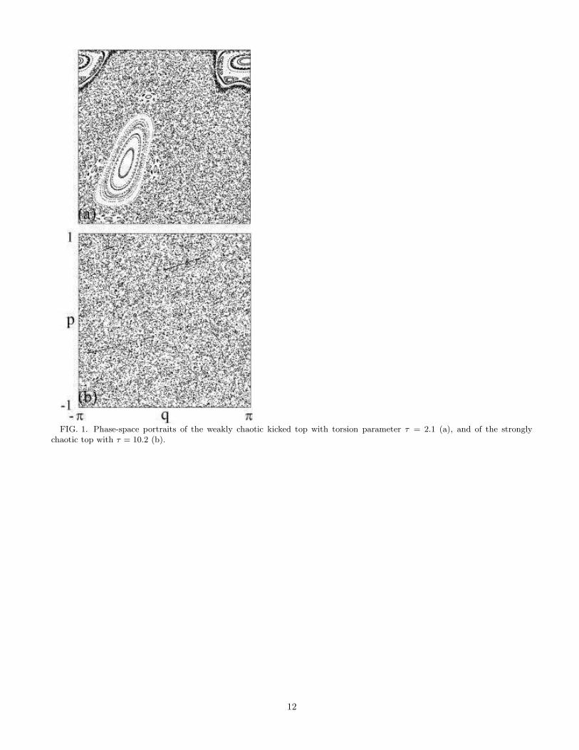
FIG. 1. Phase-space portraits of the weakly chaotic kicked top with torsion parameter τ = 2.1 (a), and of the stronglychaotic top with τ = 10.2 (b).

12

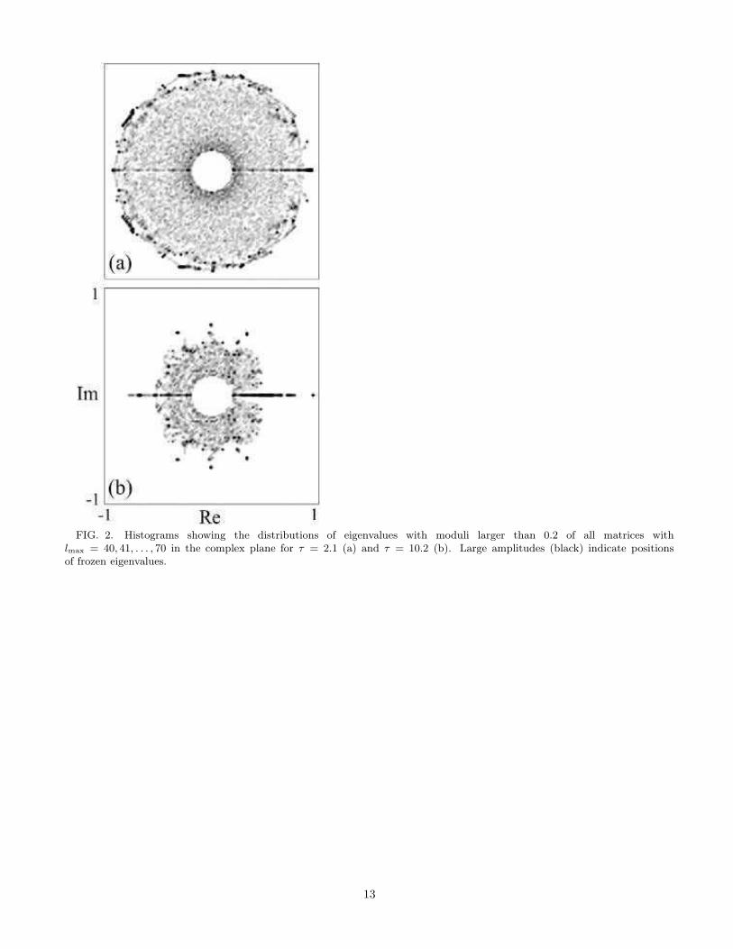
FIG. 2. Histograms showing the distributions of eigenvalues with moduli larger than 0.2 of all matrices withlmax = 40, 41, . . . , 70 in the complex plane for τ = 2.1 (a) and τ = 10.2 (b). Large amplitudes (black) indicate positionsof frozen eigenvalues.

13

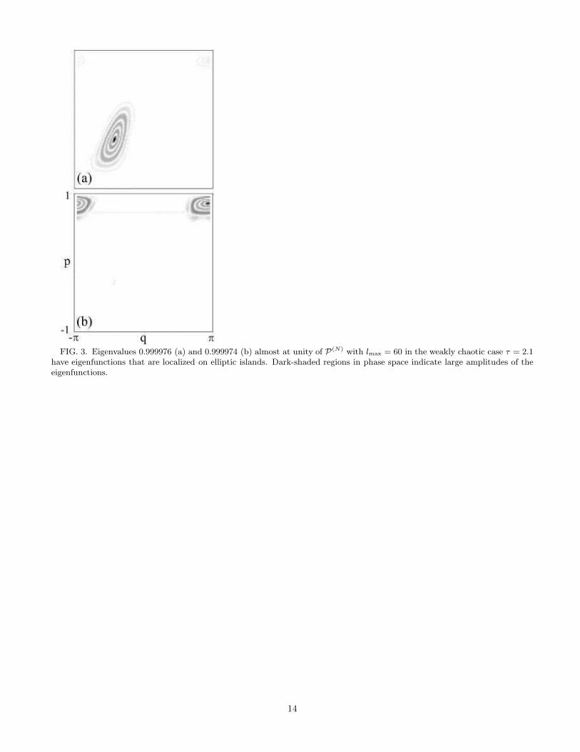
FIG. 3. Eigenvalues 0.999976 (a) and 0.999974 (b) almost at unity of P(N) with lmax = 60 in the weakly chaotic case τ = 2.1have eigenfunctions that are localized on elliptic islands. Dark-shaded regions in phase space indicate large amplitudes of theeigenfunctions.

14

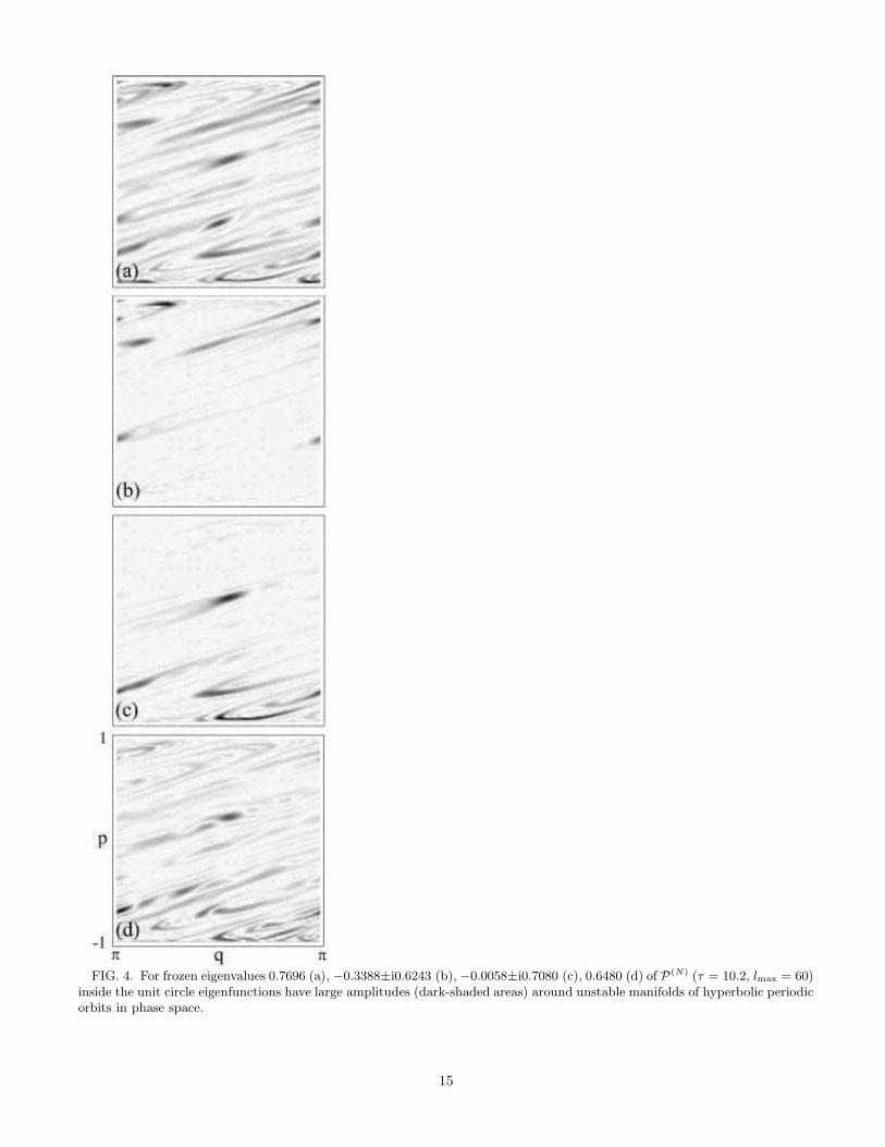
FIG. 4. For frozen eigenvalues 0.7696 (a), −0.3388±i0.6243 (b), −0.0058±i0.7080 (c), 0.6480 (d) of P(N) (τ = 10.2, lmax = 60)inside the unit circle eigenfunctions have large amplitudes (dark-shaded areas) around unstable manifolds of hyperbolic periodicorbits in phase space.

15

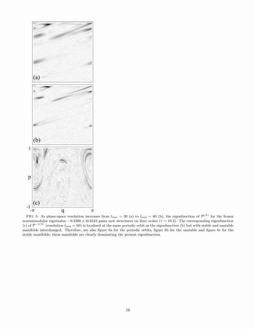
FIG. 5. As phase-space resolution increases from lmax = 30 (a) to lmax = 60 (b), the eigenfunction of P(N) for the frozen

nonunimodular eigenvalue −0.3388 ± i0.6243 gains new structures on finer scales (τ = 10.2). The corresponding eigenfunction(c) of P−1(N) (resolution lmax = 60) is localized at the same periodic orbit as the eigenfunction (b) but with stable and unstablemanifolds interchanged. Therefore, see also figure 6a for the periodic orbits, figure 6b for the unstable and figure 6c for thestable manifolds; these manifolds are clearly dominating the present eigenfunction.

16

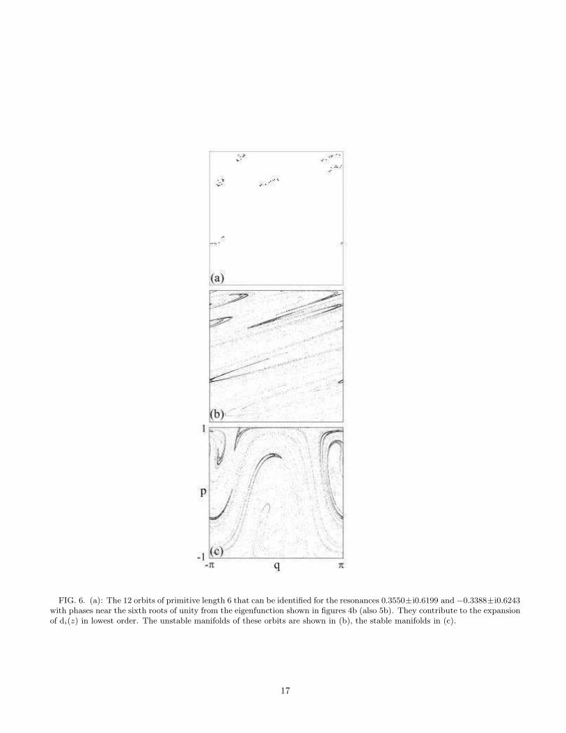
FIG. 6. (a): The 12 orbits of primitive length 6 that can be identified for the resonances 0.3550±i0.6199 and −0.3388±i0.6243with phases near the sixth roots of unity from the eigenfunction shown in figures 4b (also 5b). They contribute to the expansionof di(z) in lowest order. The unstable manifolds of these orbits are shown in (b), the stable manifolds in (c).

17

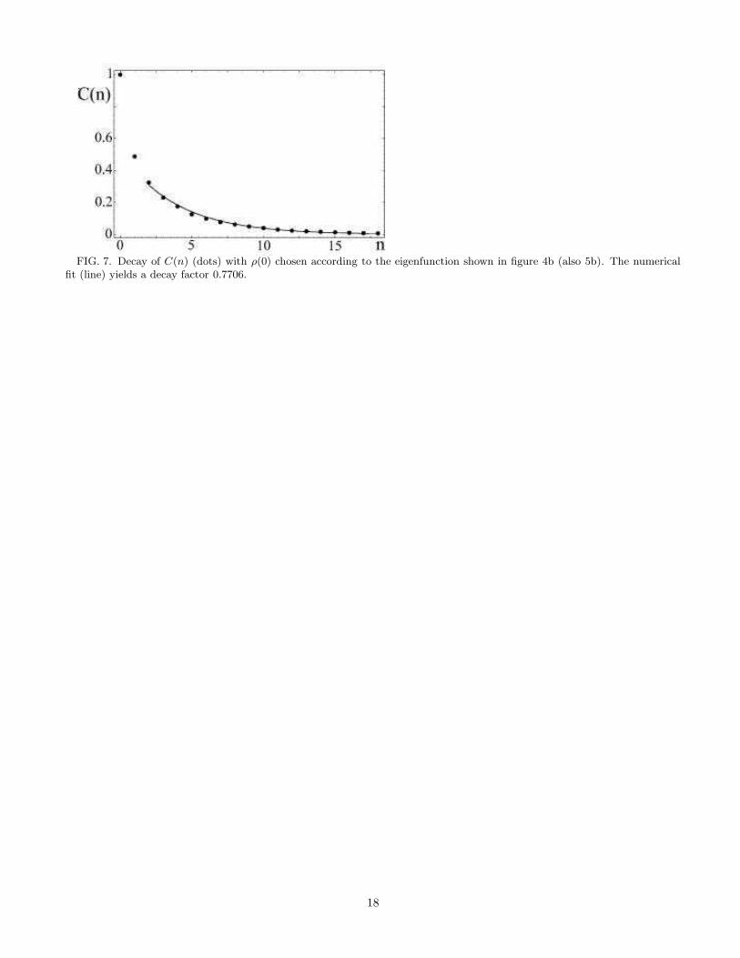
FIG. 7. Decay of C(n) (dots) with ρ(0) chosen according to the eigenfunction shown in figure 4b (also 5b). The numericalfit (line) yields a decay factor 0.7706.

18