Approximation method

Time independent• Assume that the Hamiltonian is a sum of

two terms,

• Let {Iα>} be a complete set of eigenstates of the unperturbed Hamiltonian H0 with energy eigenvalues Eα

• The eigenstates {Ia>} and eigenvalues {Ea} of the complete Hamiltonian H

H = H0 + λH1

H0 α = Eα α

H a = Ea a

Non-degenerate case• unperturbed results

• perturbed states

• Perturbation theory evaluates the eigenvalues Ea, and the coefficients cα and dβ , as power series in λ

a α Ea Eα

a = cα α + dβ ββ≠α∑

cα2+ dβ

2

β≠α∑ = 1

• To find Ea

• d is on the order of λ, and c is on the order of 1+O(λ2)

α H − Ea( ) a = 0

α H − Ea( ) a = α H0 + λH1 − Ea( ) a= cα α H0 − Ea + λH1( ) α + dβ α H0 − Ea + λH1( ) β

β≠α∑

= λcα α H1 α + cα Eα − Ea( ) + λdβ α H1 ββ≠α∑

= 0

Ea = Eα + λ α H1 α +λcα

dβ α H1 ββ≠α∑

= Eα + λ α H1 α +O λ 2( )

• To find d

• d is on the order of λ, and c is on the order of 1+O(λ2)

γ H − Ea( ) a = 0

γ H − Ea( ) a = γ H0 + λH1 − Ea( ) a= cα γ H0 − Ea + λH1( ) α + dβ γ H0 − Ea + λH1( ) β

β≠α∑

= λcα γ H1 α + dγ Eγ − Ea( ) + λdβ γ H1 ββ≠α∑

= 0

γ ≠ α

dγ = cαλγ H1 αEa − Eγ

+O λ 2( ) = λ γ H1 αEa − Eγ

+O λ 2( )

• To leading order Ea can be replaced by the unperturbed eigenvalue Eα. Hence

• This formula requires that for all β

• If the off-diagonal matrix elements of HI do not grow as the energy difference |Eα - Eβ|increases, the more "distant" a state is from the state of interest the smaller its influence will be.

a = α + βλ β H1 αEα − Eββ≠α

∑ +O λ 2( )

λ β H1 αEα − Eβ

1

• Consider the second order correction in Ea

• The leading contribution to the energy shift is the expectation value of the perturbation in the unperturbed state. The second-order term involves the other unperturbed states, and in many situations this is the leading correction because the 1st order value vanishes by symmetry.

Ea = Eα + λ α H1 α +λcα

dβ α H1 ββ≠α∑

= Eα + λ α H1 α + λ 2α H1 β

2

Eα − Eβ

+O λ 3( )β≠α∑

The validity of the perturbation expansion

• The anharmonic oscillator

Degenerate-State case

• the perturbation produces large effects on unperturbed states that have nearby neighbors

• Consider the spectrum of H0, which contains a degenerate or nearly degenerate subspace D

• Within D, no constraint is put on the magnitude of matrix elements. The problem comes from

• In view of these characteristics of the unperturbed spectrum, the unperturbed state is amended to

• Now c are on the order O(1) and d are on the order O(λ)

a = cα αα∑ + dµ µ

µ∑

λ β H1 α Eα − Eβ

• Starting from the equation

• Project it to a state |β> in D

• Project it to a state |ν> outside D

H − Ea( ) a = 0

β H − Ea( ) a = β H0 + λH1 − Ea( ) a= cα β H0 − Ea + λH1( ) α

α∑ + dµ β H0 − Ea + λH1( ) µ

µ∑

= cβ Eβ − Ea( ) + λ cα β H1 αα∑ + λ dµ β H1 µ

µ∑

= 0

β ≠ α

ν H − Ea( ) a = ν H0 + λH1 − Ea( ) a= cα ν H0 − Ea + λH1( ) α

α∑ + dµ ν H0 − Ea + λH1( ) µ

µ∑

= λ cα ν H1 αα∑ + dν Eν − Ea( ) + λ dµ β H1 µ

µ∑

= 0

• Consider equation for |ν> first

• In D, energy are similar and can be chosen as an average energy ED

• Put into the equation for |β>

λ cα ν H1 αα∑ + dν Eν − Ea( ) + λ dµ β H1 µ

µ∑ = 0

dν = λ cαν H1 αEa − Eνα

∑ +O λ 2( )

=λ

ED − Eνcα ν H1 α

α∑ +O λ 2( )

cβ Eβ − Ea( ) + λ cα β H1 αα∑ + λ dµ β H1 µ

µ∑ = 0

cβ Eβ − Ea( ) + cα λ β H1 α + λ 2β H1 µ µ H1 α

ED − Eνµ∑

⎡

⎣⎢

⎤

⎦⎥

α∑ +O λ 3( ) = 0

• This is an eigenvalue problem

• Use the projection operator

cβ Eβ − Ea( ) + cα λ β H1 α + λ 2β H1 µ µ H1 α

ED − Eνµ∑

⎡

⎣⎢

⎤

⎦⎥

α∑ = 0

−cβηβ + cα H eff( )αβα∑ = 0

β H eff α = λ β H1 α + λ 2β H1 µ µ H1 α

ED − Eνµ∑

H eff = λPH1P + λ2PH1

1− PE − H0

H1P

P = α αα∑

Example: 3-level system

H =0 0 λM0 0 λMλM λM Δ

⎛

⎝

⎜⎜

⎞

⎠

⎟⎟

P =1 0 00 1 00 0 0

⎛

⎝

⎜⎜

⎞

⎠

⎟⎟

PH1P = M1 0 00 1 00 0 0

⎛

⎝

⎜⎜

⎞

⎠

⎟⎟

0 0 10 0 11 1 0

⎛

⎝

⎜⎜

⎞

⎠

⎟⎟

1 0 00 1 00 0 0

⎛

⎝

⎜⎜

⎞

⎠

⎟⎟= 0

H1 = M0 0 10 0 11 1 0

⎛

⎝

⎜⎜

⎞

⎠

⎟⎟

H eff = λPH1P + λ2PH1

1− PE − H0

H1P

PH11− PED − H0

H1P = M2

1 0 00 1 00 0 0

⎛

⎝

⎜⎜

⎞

⎠

⎟⎟

0 0 10 0 11 1 0

⎛

⎝

⎜⎜

⎞

⎠

⎟⎟

0 0 00 0 00 0 −1 Δ

⎛

⎝

⎜⎜⎜

⎞

⎠

⎟⎟⎟

0 0 10 0 11 1 0

⎛

⎝

⎜⎜

⎞

⎠

⎟⎟

1 0 00 1 00 0 0

⎛

⎝

⎜⎜

⎞

⎠

⎟⎟

= −M 2

Δ

1 0 00 1 00 0 0

⎛

⎝

⎜⎜

⎞

⎠

⎟⎟

0 0 10 0 11 1 0

⎛

⎝

⎜⎜

⎞

⎠

⎟⎟

0 0 00 0 01 1 0

⎛

⎝

⎜⎜

⎞

⎠

⎟⎟

= −M 2

Δ

1 1 01 1 00 0 0

⎛

⎝

⎜⎜

⎞

⎠

⎟⎟

Heff = −M 2

Δ

1 1 01 1 00 0 0

⎛

⎝

⎜⎜

⎞

⎠

⎟⎟

EA = 0ES = −2M

2 Δ

EA = 1 − 2( ) 2

ES = 1 + 2( ) 2

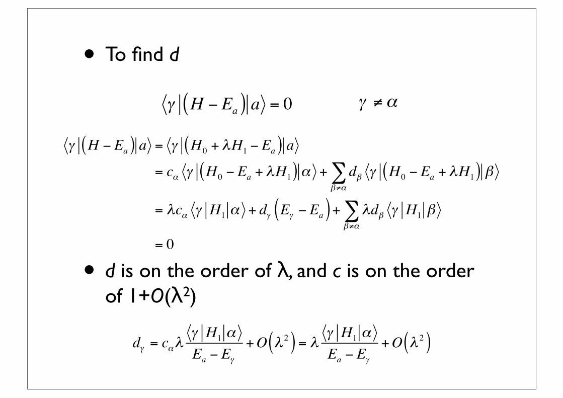
Time dependent

• The Hamiltonian of the system is

• where V(t), called the perturbation, may be time-dependent

• The state of interest, lΨi(t)>, is a solution of the complete Schrodinger equation

H = H0 +V t( )

i ∂∂t

Ψ i t( ) = H0 +V t( )⎡⎣ ⎤⎦ Ψ i t( )

• This solution is to evolve out of a solution lΦi(t)> of the unperturbed Schrodinger equation,

• where lΦi(t)> is a solution of

Ψ i t( ) → Φi t( ) when t→−∞

i ∂∂t

Φi t( ) = H0 Φi t( )

• The first type of problem is one where V(t) is explicitly time-dependent. It is "turned on," at t =0, and the initial state lΦi(t)> is a stationary state of H0.

• For t > 0 we wish to know the probability for the system to be in some other stationary state lΦf(t)> of H0.

• example : an atom in its ground state which is subjected to an applied electromagnetic field.

• The second example : the collision of a particle with a time-independent potential V of finite range.

• a distant detector Df which, in effect, asks for the probability that the state has evolved into the state lΦf(t)>

V

initial state lΦi(t)>free-particle wave packet

detector Df

lΦf(t)>

scattered state

• This transition probability is

• Pif is closely related to such observable quantities as scattering cross sections, but to make this connection important details remain to be settled.

• the term transition amplitude can be introduced

Pi→ f t( ) = Φ f t( ) Ψ i t( )2

Ai→ f t( ) = Φ f t( ) Ψ i t( )

• lowest-order time-dependent perturbation

• To solve this equation, consider first a similar ordinary differential equation

• The solution with initial condition

i ∂∂t− H0

⎛⎝⎜

⎞⎠⎟Ψ i t( ) =V t( ) Ψ i t( ) V t( ) Φi t( )

i ddt−C⎛

⎝⎜⎞⎠⎟ψ t( ) = s t( )

ψ t( ) = φ t( )− i e− iC t− ʹ′t( )s ʹ′t( )−∞

t

∫ d ʹ′t

ψ t( ) = φ t( ) when t→−∞

sufficiently rapidly. s t( )→ 0 as t→−∞

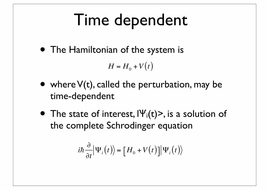
• because H0 commutes with itself

• The transition amplitude Ψ i t( ) = Φi t( ) −

i

e− iH0 t− ʹ′t( ) V ʹ′t( ) Φi ʹ′t( )−∞

t

∫ d ʹ′t

Ai→ f t( ) = Φ f t( ) Φi t( ) −

i

Φ f t( ) e− iH0 t− ʹ′t( ) V ʹ′t( ) Φi ʹ′t( )−∞

t

∫ d ʹ′t

• Consider an atom exposed to a uniform time-dependent electric field E(t), in which case the perturbation V(t) is -E(t)d, where d is the operator that corresponds to the component of the atom's electric dipole moment parallel to E.

• this problem has the form V(t)=f(t)Q where f(t) is a numerical function and Q some observable of the system.

• the initial and final states are eigenstates of H0,

• The transition probability

Φi, f t( ) = e

− iEi , f t Φi, f

Pi→ f t( ) = Φ f t( ) Ψ i t( )2=12

Φ f t( ) e− iH0 t− ʹ′t( ) V ʹ′t( ) Φi ʹ′t( )−∞

t

∫ d ʹ′t2

=12

d ʹ′t eiE f t e− iEi ʹ′t e− iE f t− ʹ′t( ) f ʹ′t( ) Φ f Q Φi−∞

t

∫2

=12

Φ f Q Φi

2d ʹ′t ei E f −Ei( ) ʹ′t f ʹ′t( )

−∞

t

∫2

=12

Φ f Q Φi

2F ω fi ,t( )

2

• Consider a periodic perturbation f(t) = sinνt that turns on at t = 0,

F ω ,t( ) = d ʹ′t eiω ʹ′t sinν ʹ′t0

t

∫ =12i

d ʹ′t ei ω+v( ) ʹ′t − ei ω−v( ) ʹ′t⎡⎣ ⎤⎦0

t

∫

=12ei ω−v( )t −1ω −ν

−12ei ω+v( )t −1ω +ν

= iei ω−v( )t 2 sinω −ν

2t

ω −ν− iei ω+v( )t 2 sinω +ν

2t

ω +ν

• the perturbation is resonant, i.e., has a frequency ν that is close to one of the excitation frequencies ωfi.

F ω ,t( ) 2 iei ω−v( )t 2 sinω −ν

2t

ω −ν

2

+ 2Re ei ω−v( )t 2e− i ω+v( )t 2( )sinω −ν

2t

ω −ν

sinω +ν2

t

ω +ν

=sin2 ω −ν

2t

ω −ν( )2+ 2cosωt sinωt

sinω −ν2

t

ω ω −ν( )

• At resonance,

• Assume the more realistic form of perturbation

Pi→ f t( ) =

12

Φ f Q Φi

2 sin2 ω −ν2

t

ω −ν( )2

V t( ) =Qe− t τ sinνt

Pi→ f t( ) =

142

Φ f Q Φi

2 1ω −ν( )2 +1 τ 2 t τ

The Golden Rule

• Consider the second type of problem

• Unless the scattering is in the exact forward direction, only the second term in contributes,

• first assume that for some very large but finite time - T in the past,

Ai→ f t( ) = −

iΦ f V Φi e− iω fi ʹ′t d ʹ′t

−∞

t

∫

Ai→ f T( ) = − i

Φ f V Φi e− iω fi ʹ′t d ʹ′t

−T

T

∫

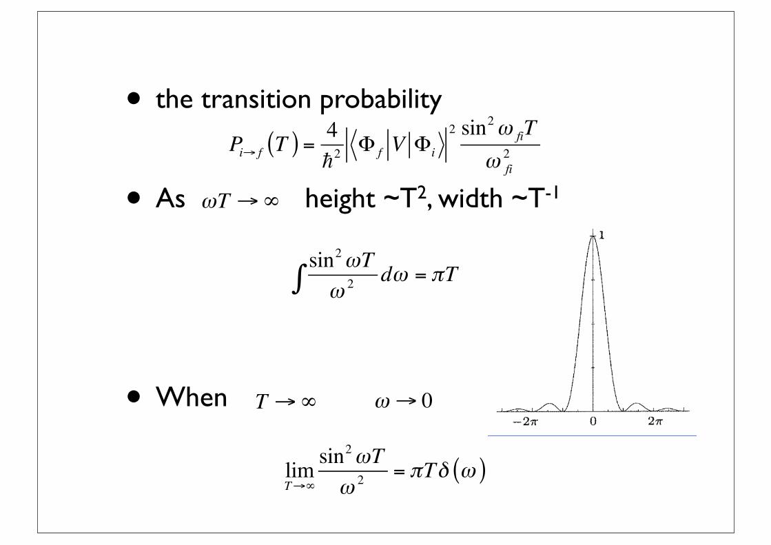
• the transition probability

• As height ~T2, width ~T-1

• When

Pi→ f T( ) = 4

2Φ f V Φi

2 sin2ω fiTω 2

fi

sin2ωTω 2 dω∫ = πT

ωT →∞

T →∞ ω → 0

limT→∞

sin2ωTω 2 = πTδ ω( )

• The transition probability

• the steady transition rate

• We call this formula Golden rule

Pi→ f T →∞( ) = 4π

Φ f V Φi

2Tδ Ef − Ei( )

dPi→ f

dt=2π

Φ f V Φi

2δ Ef − Ei( )