HEDONIC PRICING MODEL FOR REAL PROPERTY ...

CIVIL AND ENVIRONMENTAL ENGINEERING REPORTS E-ISSN 2450-8594 CEER 2019; 29 (3): 034-047

DOI: 10.2478/ceer-2019-0022 Original Research Article

HEDONIC PRICING MODEL FOR REAL PROPERTY VALUATION VIA GIS - A REVIEW

Zubeida ALADWAN, Mohd Sanusi S. AHAMAD1 School of Civil Engineering Campus, Universiti Sains Malaysia, Malaysia

A b s t r a c t

Hedonic pricing models in real property valuation have been frequently applied in many research studies and projects since it was introduced by Rosen in 1974. The development of Geographic Information Systems (GIS) in the recent decades has gradually supports the usage of hedonic model in the spatial data pricing model studies. Beside the basic advantages of GIS to position properties in terms of their geographic coordinates, it has the capabilities of dealing with reasonable amount of data, and wide choices of analysis that make it powerful tool to facilitate the building and implementation of the hedonic models within its framework. Many studies have employed GIS in real property valuation in their present work and for the future prediction. This paper reviews the works of literature on the GIS applications in the real property valuation employing the hedonic pricing models.

Keywords: Real property valuation, Building variables, Regression analysis, Hedonic pricing models, GIS

1. INTRODUCTION

The conventional real property valuation system in most of the assets departments and institutions is costly, time consuming, received frequents public complaints for its lack of transparency and subjectivity. Therefore, efforts had been exerted to improve the value estimation process making it fast and enhance its reality and 1 Corresponding author: Universiti Sains Malaysia, School of Civil Engineering, Engineering Campus, 14300 Nibong Tebal, Penang, Malaysia, e-mail: [email protected], tel: +6045996277


35

ability to reflect the people willingness to pay. However, the process of collecting information for the real property valuation requires serious effort that consumed time and cost. Subjectiveness of the appraisers in this process affects the probity and reality of the value estimation. Hedonic pricing is considered as the “revealed preference method” as it is based on the actual real behaviour, rather than intended one. It does not require previous judgments, comparative prices, or income information in order to value the real property as in the conventional methods. It requires some reasonable amount of pricing data, and strong statistical and analytical tools that can be facilitated and simplified. GIS-Hedonic pricing-based models is expected to help in this direction since it provides varied capabilities of managing and analysing buildings data specially that of locational dimension. The common procedures being practiced over the last ten years generally started with the selection of the variables to be valued accordingly by the real property, then applying the statistical regression method to correlate prices to its corresponding parameters, and finally building the hedonic model for further value estimations. This article reviews specific studies on the utilisation of GIS application in the hedonic pricing models over the last decade. The aims are to find the gaps that can enhance the valuation procedure in GIS-hedonic pricing model that focussed on the reliability, accuracy, timesaving and effort.

2. GIS BASED HEDONIC PRICING

Although there have been many attempts to use GIS in the hedonic pricing model, but the scope of the previous work was generally to locate the buildings, to calculate certain locational variable related metrics and to generate spatial based parameters. This signified the difficulty of managing the real property data and the solid statistical background needed for such model. The GIS capability is still not fully being explored and utilized.

The hedonic pricing-based valuation procedures The approach for determining the property value is hedonic. A hedonic valuation model depends on the idea that a property buyer values the characteristics of the property, rather than the property in total. This means that the property prices reflect the prices of the property characteristics, which include the locational variables. When a regression model is applied, the value of each property parameter or characteristic can be determined. The common workflow of the past research methodologies reviewed is generalized in Figure 1.

36 Zubeida ALADWAN, Mohd Sanusi S. AHAMAD

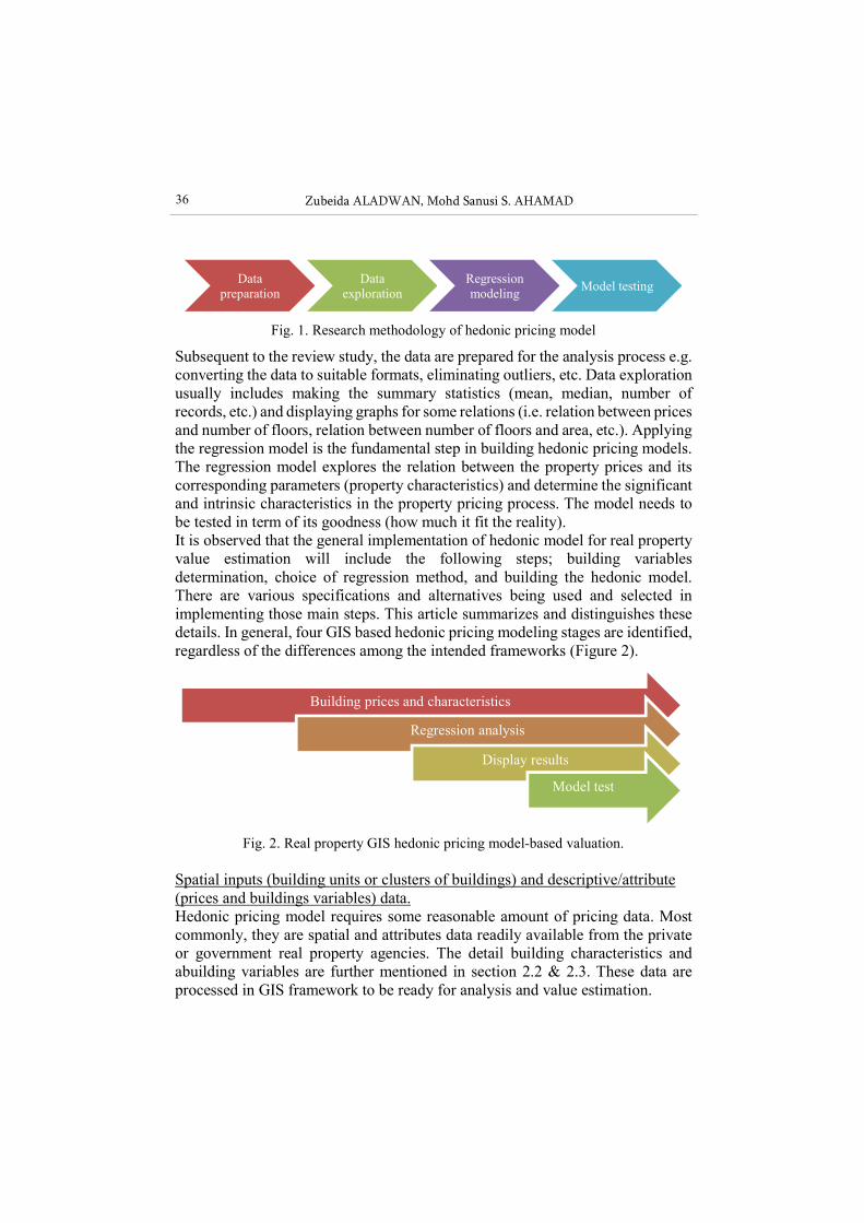
Fig. 1. Research methodology of hedonic pricing model

Subsequent to the review study, the data are prepared for the analysis process e.g. converting the data to suitable formats, eliminating outliers, etc. Data exploration usually includes making the summary statistics (mean, median, number of records, etc.) and displaying graphs for some relations (i.e. relation between prices and number of floors, relation between number of floors and area, etc.). Applying the regression model is the fundamental step in building hedonic pricing models. The regression model explores the relation between the property prices and its corresponding parameters (property characteristics) and determine the significant and intrinsic characteristics in the property pricing process. The model needs to be tested in term of its goodness (how much it fit the reality). It is observed that the general implementation of hedonic model for real property value estimation will include the following steps; building variables determination, choice of regression method, and building the hedonic model. There are various specifications and alternatives being used and selected in implementing those main steps. This article summarizes and distinguishes these details. In general, four GIS based hedonic pricing modeling stages are identified, regardless of the differences among the intended frameworks (Figure 2).

Fig. 2. Real property GIS hedonic pricing model-based valuation.

Spatial inputs (building units or clusters of buildings) and descriptive/attribute (prices and buildings variables) data. Hedonic pricing model requires some reasonable amount of pricing data. Most commonly, they are spatial and attributes data readily available from the private or government real property agencies. The detail building characteristics and abuilding variables are further mentioned in section 2.2 & 2.3. These data are processed in GIS framework to be ready for analysis and value estimation.

Data preparation

Data exploration

Regression modeling

Model testing

Building prices and characteristics

Regression analysis

Display results

Model test


37

Regression analysis within or out of a GIS software framework. Hedonic models are most commonly estimated using regression analysis which is model for estimating the relationships between variables, usually a dependent variable and one or more independent variables. Using a regression model the value of each property parameter or characteristic can be determined. In real property studies hedonic regression function can de expressed as in Eq. (1)

p= f (x1, x2, …, xn) (1)

Where p is the property price, and x1, x2, …, xn are the property characteristics. f could be linear or nonlinear function. The hedonic regression function often employed to study the property multiple factors effects on its final price, or in another word the contribution of each factor on the final price. It decomposes the property being studied into its constituent characteristics and estimates the contributory value of each characteristic. The good needs to be able to break down into its constituent parts that for each there is market value. The mostly adopted regression method is provided in section 3. Display results The results of the regression analysis can be presented in the form of reports and maps inside GIS. The results and the diagnostics will be able to show the coefficients values of each property parameters. It can show the contribution of each characteristics in the price and allow to determine the dominant ones. Hence, the future prediction of prices will be possible in the integrated GIS hedonic model. Model test For any statistical method there are assumptions to be made. The validity of the GIS based hedonic models are measured by how well the model assumptions are met. Many statistical procedures are “robust”, which means that only extreme violations from the assumptions weaken the ability to draw valid conclusions. Section 4 of this paper provides a brief value estimation model needed to be tested in terms of the model fit, model autocorrelation, and model goodness.

Most commonly used building characteristics The three main categories of the building variables commonly used in the hedonic model are: (1) Structural characteristics, (2) Neighbourhood characteristics, and (3) Locational characteristics [1], [2], [8], [10], [13], [16], [17], [18], [19]. However, some studies merely concentrate on certain building parameters such as the effects of green spaces in contributing the property prices [10,16], whereas Cellmer [3] put interests only on the effect of noise intensity. Other than the


structural and locational variables, the socio demographic, socio economic and social variables where considered by others in their work [4,7]. In addition to the structural variables, Lehner [12] concentrate on the locational variables represented by the distances to the point of interests, POIs (i.e. education, transport, work, etc.). Lu et al. [14] uses limited set of structural variables together with the regional variable comprising of the percentage workforce in professional or managerial occupations in the census enumeration district where the house is located. Eboy and Samat [5] utilised a limited set of variables in building the hedonic model in their work of. GIS was used to obtain the property location to the nearest: public institutions, tourism centres, public recreations, public facilities, commercial areas, government offices and religious centres. Other than the three mentioned building variables, Cebula [2] considered other factor such as whether the property was designated as the national historic landmark or located in the historical district. Whereas, Lozano and Anselin [13] focused on performance of different model specifications used in the automated valuation rather than the effect of the building parameters itself on the final prices. Ottensmann et al. [17] put interests in the locational measure in representing the location accessibility, along with the buildings parameters coefficients. Yang, et al. [23] used three categories of building variables; structural covariates, temporal covariates, and neighborhood covariates (i.e. whether the resident is within the major road ring or otherwise). Oud [18] includes the property view in the model building using ESRI GIS software viewshed tool. His study found out that most of the automated valuation models (AVM) take only the objective property characteristics and transaction information to fit the statistical prediction model. Hence, it is less detailed than the one with additional subjective information, but highly cost efficient. The main input for automated models is structural property characteristics such as size, age and type of property. In AVM minor attention is paid towards locational and quality characteristics since its methodology lacks physical inspections. Nonetheless, the usage of GIS will help obtaining such variables without physical inspection.

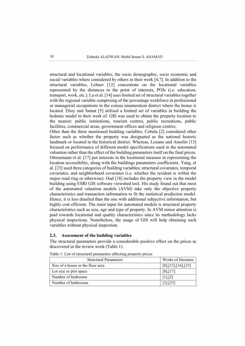
Assessment of the building variables The structural parameters provide a considerable positive effect on the prices as discovered in the review work (Table 1).

Table 1: List of structural parameters affecting property prices

Structural Parameters Works of literature

Size of a house or the floor area [8],[12],[16],[23]

Lot size or plot space [8],[17]

Number of bedrooms [1],[2]

Number of bathrooms [2],[23]


39

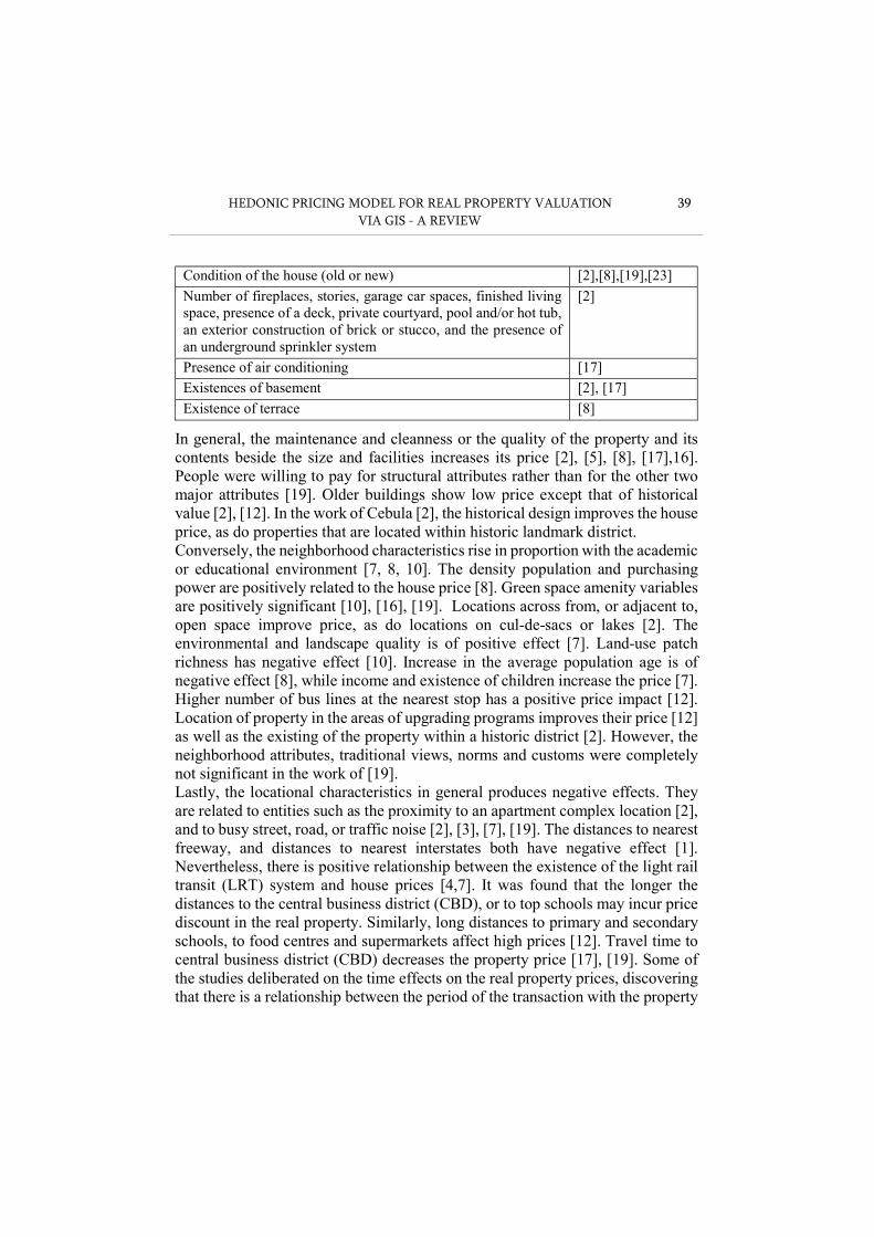
Condition of the house (old or new) [2],[8],[19],[23]

Number of fireplaces, stories, garage car spaces, finished living space, presence of a deck, private courtyard, pool and/or hot tub, an exterior construction of brick or stucco, and the presence of an underground sprinkler system

[2]

Presence of air conditioning [17]

Existences of basement [2], [17]

Existence of terrace [8]

In general, the maintenance and cleanness or the quality of the property and its contents beside the size and facilities increases its price [2], [5], [8], [17],16]. People were willing to pay for structural attributes rather than for the other two major attributes [19]. Older buildings show low price except that of historical value [2], [12]. In the work of Cebula [2], the historical design improves the house price, as do properties that are located within historic landmark district. Conversely, the neighborhood characteristics rise in proportion with the academic or educational environment [7, 8, 10]. The density population and purchasing power are positively related to the house price [8]. Green space amenity variables are positively significant [10], [16], [19]. Locations across from, or adjacent to, open space improve price, as do locations on cul-de-sacs or lakes [2]. The environmental and landscape quality is of positive effect [7]. Land-use patch richness has negative effect [10]. Increase in the average population age is of negative effect [8], while income and existence of children increase the price [7]. Higher number of bus lines at the nearest stop has a positive price impact [12]. Location of property in the areas of upgrading programs improves their price [12] as well as the existing of the property within a historic district [2]. However, the neighborhood attributes, traditional views, norms and customs were completely not significant in the work of [19]. Lastly, the locational characteristics in general produces negative effects. They are related to entities such as the proximity to an apartment complex location [2], and to busy street, road, or traffic noise [2], [3], [7], [19]. The distances to nearest freeway, and distances to nearest interstates both have negative effect [1]. Nevertheless, there is positive relationship between the existence of the light rail transit (LRT) system and house prices [4,7]. It was found that the longer the distances to the central business district (CBD), or to top schools may incur price discount in the real property. Similarly, long distances to primary and secondary schools, to food centres and supermarkets affect high prices [12]. Travel time to central business district (CBD) decreases the property price [17], [19]. Some of the studies deliberated on the time effects on the real property prices, discovering that there is a relationship between the period of the transaction with the property


prices. Cebula [2] noticed that the real sales price of residential properties that closed during May or July tends to be higher.

Real property price type and sample size The actual transaction prices were used in many studies. Some of them are of reasonable sample size, for example Cebula [2] employed 2888 sample prices in 2000-2005 and transformed it to 2005 price rate, Helbich [8] used 3887 purchased prices of homes in 1998-2009, and Ottensmann et al. [17] considered 8,772 recorded sales in 1999. The work of Noor et al. [16] was limited to the average semi-detached unit house prices of per residential district of 50 samples. Likewise, Randeniya et al. [19] uses 50 samples of houses prices (2008-2013) in their work. The real transaction prices of 124 housing clusters in 2004 were used in Kong et al. [10] and the samples varies from 6351 to around 46000 residents (private and governmental). In Lehner [12], the samples in the study area differ from market to market and the new pricing models built for (2010- 2011) were based on the asking prices, transaction prices, and asking rentals from online sources. Cellmer [3] study the effect of noise intensity on the transaction prices from 2008 to 2010 period using 1100 sample apartments. Dziauddin [4] and Yang et al. [23] worked using 1600 and 1350 residential houses respectively using old transaction prices relative to the study year. Dziauddin [4] used samples in (2004-2007) but the socioeconomic and social variables data were constructed from 1990 and 2000 census. The sample prices of Yang et al. [23] were taken from 1996 to 2015. Lu et al. [14] employed 2108 single house data (sale prices) that were registered in 2001. A large sample of 5524 residential properties (except apartments and condominiums) were considered in the work of Eboy and Samat [5], using the old data property rating value of 1997. A total of 14000 house prices were used by Lozano-et al. [13] but limited to the house prices taken from books for tax purposes (lower price) over the time period of 2002-2007 and transforming it to 2008 prices. Bujanda [1] built three pricing models namely the total value of the residents (residential properties), the improvement value, and the land value. The study employed 198,574 single family properties obtained from the certified cadastral parcel records, where it was separated into the three mentioned models. It can be concluded that the age of property valuation data is not critical if both the prices and their corresponding parameters are compatible. The problem only reveals when the prices values (the independent variable) are taken in a period much older than the recent characteristics of the property. The compatibility of time with data sufficiency are of high interest in the research that predict people willingness to pay via hedonic pricing models.


41

3. REGRESSION METHODS

The ordinary least square (OLS) is the dominant method in the implementation of regression analysis [2], [10], [13], 17]. OLS is considered as global method that produces constant coefficient over the whole study area and does not take account the autocorrelation and heterogeneity (spatial effects) problems. Local regression methods are most preferred especially for the spatial building variables or the variables that are expected to have different effects along different locations. Geographic Weighted Regression (GWR) is a local regression method that allows coefficients to vary along the study areas. It was used by several researches [1, 3, 4, 5]. GWR has the possibility to be implemented fully inside many vector-based GIS frameworks such as ArcGIS, QGIS, MapInfo Professional, Geomedia, etc. Currently, the ArcGIS tool has it in linear regression version. The Mixed OLS-GWR (MGWR) method was employed in the work of Helbich et al. [8], but the computational burdens have limited the usage of GWR-MGWR for large data set especially when GIS was not used. Yang et al. [23] integrated the model from GWR with semi supervised methods. Since this method used unknown prices regression, not all the explanatory variables vary over space. Therefore, this mix method requires further investigation. In the similar manner, Lu et al. [14] used OLS as the elementary step for further GWR estimation. In summary, GIS can aid in applying the regression analysis and building the hedonic model itself beside the traditional usage of locating the buildings and determining some of their spatial related variables. Having a functioning GIS based hedonic pricing model framework will be a value added and recognized contribution in the field of real property valuation.

3.1. Most commonly used hedonic model equations There are different functional specifications of hedonic equations found in the literatures. The semi log regression was the most preferable and commonly used equation in building the computerized hedonic model for its simplicity in interpreting the results, and its ability to accept categorical variables [2], [10], [12], [17], and 19]. In the semi-log models either the dependent variable or the explanatory variables are transformed. The regression coefficients of semi-log models can be interpreted as the relative change of the dependent variable given a change of the explanatory variable. Alternatively, the studies by [4], [8], and [12] used the log-log regression, in which both sides of the regression function are logarithmized. The log-log coefficients can be interpreted as elasticities. Elasticities are approximately the change of the dependent variable in percent if the explanatory variable changes one percent.The simplest mathematical linear regression was employed by [1], [3], [5], [10], [14], [16], and [24].


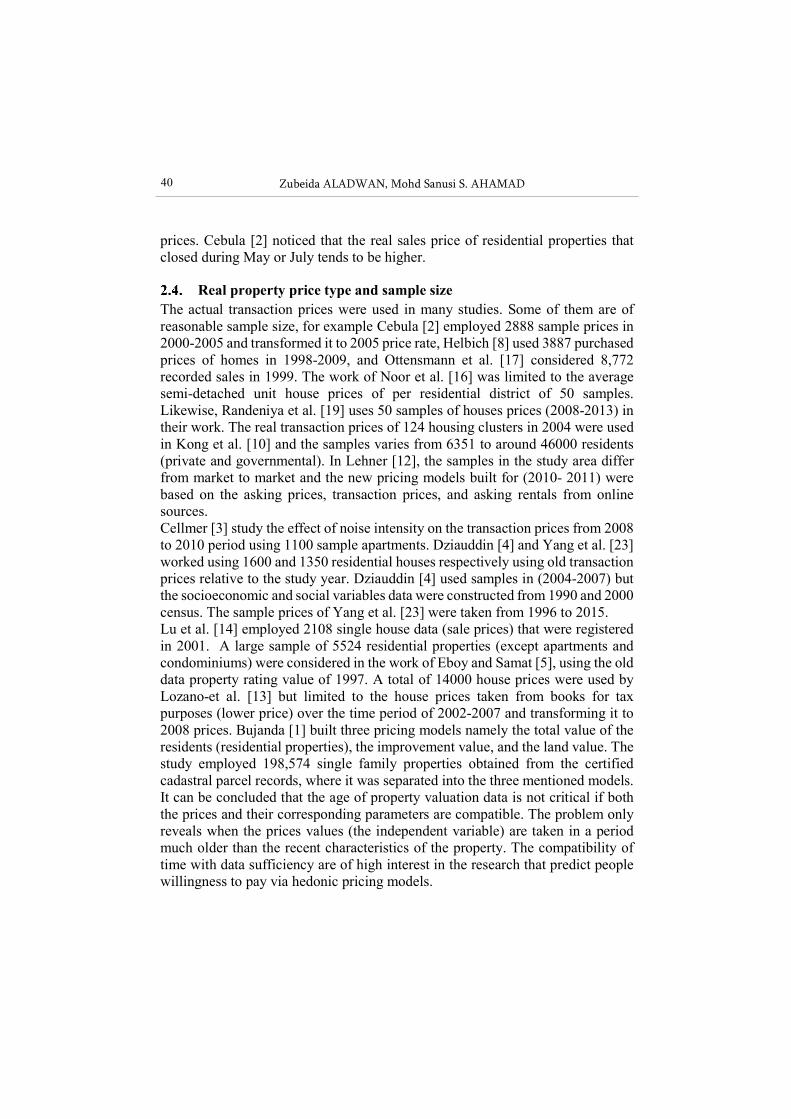
While, both the linear and logistic regression models were employed in the study of Giaccaria and Frontuto [7], complementing GWR and standard double bounded contingent valuation. The contingent valuation interested ask people to directly report their willingness to pay (WTP) to obtain a specified good, or willingness to accept (WTA) to give up a good, rather than inferring them from observed behaviors in regular marketplaces. The hedonic model depends on the real behaviour of people rather than their opinions. Linear regression model data used a straight line where the random variable, Y (response variable) is modeled as a linear function of another random variable, X (predictor variable). Instead, in the logistic regression models, the probability of the events in bivariate which essentially occurs act as the linear function of a set of dependent variables. Figure 3 that explains the difference between the graph of linear regression model (left) and graph of logistic regression model (right).

Fig. 3. Linear regression model (left graph) and Logistic regression model (right graph)

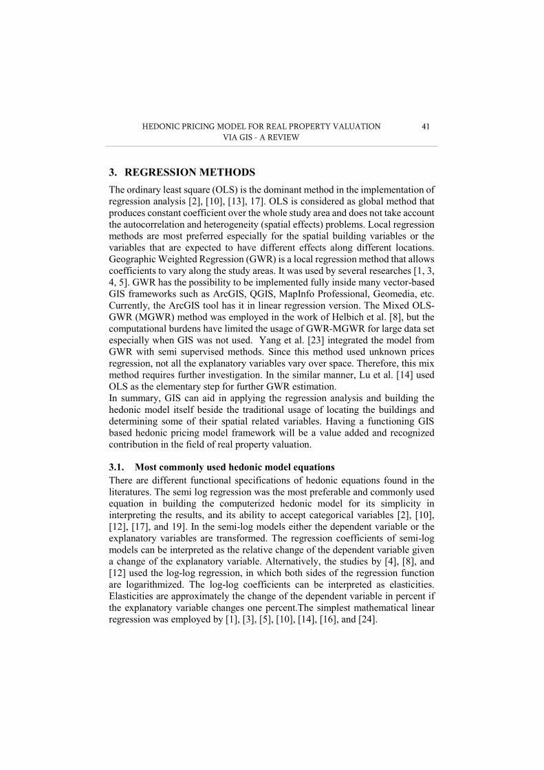
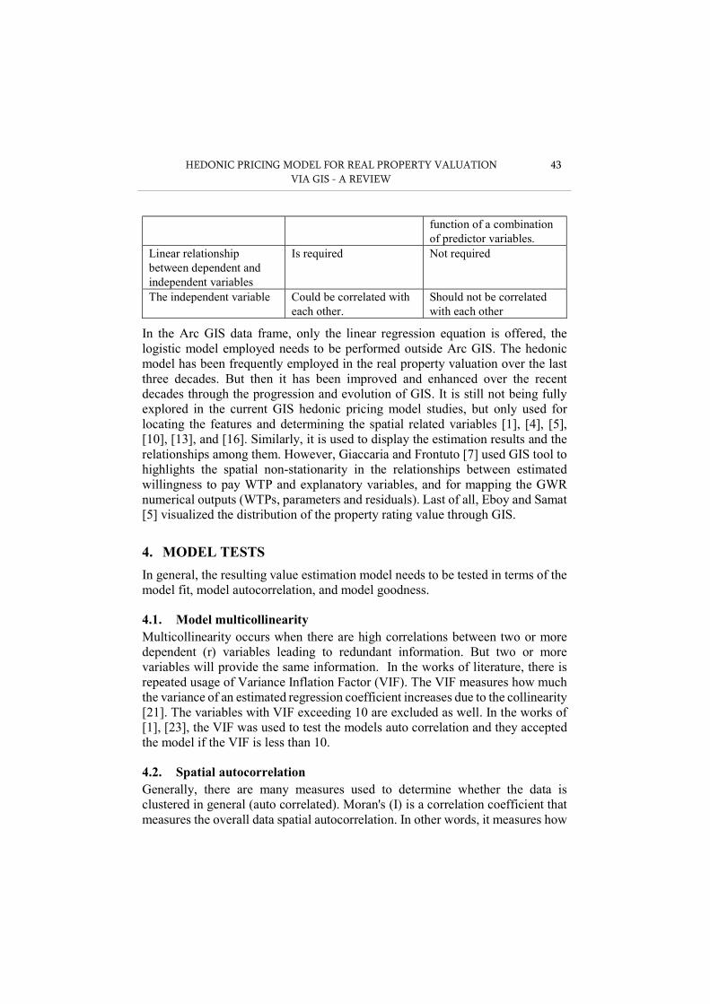
The logistic regression is used when the dependent variable is of binary nature, while linear regression is used when the regression line is linear, and the dependent variable is continuous. This is considered as the essential differences between them. Table 2 described the key differences between the linear and logistic regression.

Table 2. The key differences between the linear regression model and the logistic regression model. (Tech Differences, 2018)

Basis for comparison Linear regression Logistic regression

Basic The data is modeled using a straight line.

The probability of some obtained event is represented as a linear


43

function of a combination of predictor variables.

Linear relationship between dependent and independent variables

Is required Not required

The independent variable Could be correlated with each other.

Should not be correlated with each other

In the Arc GIS data frame, only the linear regression equation is offered, the logistic model employed needs to be performed outside Arc GIS. The hedonic model has been frequently employed in the real property valuation over the last three decades. But then it has been improved and enhanced over the recent decades through the progression and evolution of GIS. It is still not being fully explored in the current GIS hedonic pricing model studies, but only used for locating the features and determining the spatial related variables [1], [4], [5], [10], [13], and [16]. Similarly, it is used to display the estimation results and the relationships among them. However, Giaccaria and Frontuto [7] used GIS tool to highlights the spatial non-stationarity in the relationships between estimated willingness to pay WTP and explanatory variables, and for mapping the GWR numerical outputs (WTPs, parameters and residuals). Last of all, Eboy and Samat [5] visualized the distribution of the property rating value through GIS.

4. MODEL TESTS

In general, the resulting value estimation model needs to be tested in terms of the model fit, model autocorrelation, and model goodness.

4.1. Model multicollinearity Multicollinearity occurs when there are high correlations between two or more dependent (r) variables leading to redundant information. But two or more variables will provide the same information. In the works of literature, there is repeated usage of Variance Inflation Factor (VIF). The VIF measures how much the variance of an estimated regression coefficient increases due to the collinearity [21]. The variables with VIF exceeding 10 are excluded as well. In the works of [1], [23], the VIF was used to test the models auto correlation and they accepted the model if the VIF is less than 10.

4.2. Spatial autocorrelation Generally, there are many measures used to determine whether the data is clustered in general (auto correlated). Moran's (I) is a correlation coefficient that measures the overall data spatial autocorrelation. In other words, it measures how


one feature is similar to the other feature that is located near it. If objects are attracted to its surrounding objects, it means that the observations are not independent [12]. Moran’s is the most common measure for spatial autocorrelation [5], [8], [12], [14]. The Getis-Ord's Gi test was explored by Bujanda [1]. In the ArcGIS used, the hot spot analysis tool calculates the Getis-Ord Gi* statistic for each feature in a dataset. It shows where the features with either high or low values clustered spatially. The algorithm searches each feature within the context of neighbouring features. Therefore, to be a statistically significant hot spot, a feature will have a high value and surrounded by other features with high values as well [6].

4.3. Model goodness For the comparison purposes, the sum of squared errors (SSE) is used to test the model fit. A well fit model is related to smaller SSE value [12]. In addition to the model coefficients, other computations that are required includes the standard error (SE) i.e. the average difference between the estimated coefficient and the true coefficient, the coefficients for standardized variables and the t-statistic. The higher the absolute value the stronger the impact of the variable. The t-test is used to examine the hypothesis that a regression coefficient is equal to zero. Higher t-values indicate a higher precision of the estimated parameter [12]. The Akaike’s information criterion (AIC) and R2 were used to test the model goodness of fit [1],[5],[8],[23]. The R2 is the most common measure for the goodness of fit of the regression line. The values range from 0 to 1, i.e. values nearer to 1 indicate a better fit. The AIC is an estimator of the relative quality of the models for a certain data set. The small AIC value indicates the model is better.

5. CONCLUSIONS

As mentioned earlier, the GIS has not yet been fully explored in the study of the hedonic pricing model. Beside its ordinary role of displaying the results and obtaining some locational variables, the GIS functions can be used for further analysis by developing the appropriate steps in building, applying, and testing the hedonic pricing model. It has the capabilities of dealing with reasonable amount of data, and wide choices of analysis such as spatial autocorrelation, spatial dependence, proximity and average distance that make it powerful tool to facilitate hedonic model within its framework. GIS with hedonic model helps in making suitable location decisions for neighborhood or housing development, commercial buildings, schools or other facilities located based on the identified prime attributes. Although the GWR regression analysis is independently performed when the spatial problems (variable autocorrelation and heterogeneity)


45

are considered, it has the possibility to be built in the GIS frameworks. The review focussed on the residential property buildings data that were of reasonable small sample size (either old or new). As such, other types of building can be considered for hedonic price modeling through GIS. The hedonic price model dealing with the property type is recommended and can have a predictable effect in the real property pricing. Having GIS explicit spatial autocorrelation in the hedonic model has masked the true elasticity of property price to the important variables. It enabled more accurate estimation of the implicit price of the variables and more reliable statistical inference of property markets. It is recommended for the governmental institutions to have an ‘up to date’ property’s data available for value estimation, where the pricing process run parallel with the transaction implementation, e.g., whenever the property owners apply for a certain transaction, they are requested to provide their property data. Realistically, the latest pricing data can be offered for further analysis and building hedonic pricing models. The real property department can determine variables according to the estimated price and used in the regression analysis to determine the most dominant to be included in the hedonic pricing model.

REFERENCES

1. Bujanda, A and Fullerton, TM 2017. Impacts of transportation infrastructure on single-family property values. Applied Economics. 49(1) 1-17.

2. Cebula, R 2009. The hedonic pricing model applied to the housing market of the city of savannah and its Savannah historic landmark district. The Review of Regional Studies. 39(1) 9-22.

3. Cellmer, R 2011. Spatial Analysis of The Effect of Noise on The Prices and Value of Residential Real property. Geomatics And Environmental Engineering. 5(4) 13-28.

4. Dziauddin, M 2009. Measuring The Effects of The Light Rail Transit (LRT) System on House Prices in the Klang Valley, Malaysia. Ph.D. Thesis, Newcastle University, 517.

5. Eboy, O and Samat, N 2015. Modeling property rating valuation using Geographical Weighted Regression (GWR) and Spatial Regression Model (SRM): The case of Kota Kinabalu, Sabah. Malaysian Journal of Society and Space.. 11(11) 98-109.

6. Esri, 2005: How Hot Spot Analysis: Getis-Ord Gi* (Spatial Statistics) works, [http://resources.esri.com/help/9.3/arcgisengine/java/gp_toolref/spatial_statistics_tools/how_hot_spot_analysis_colon_getis_ord_gi_star_spatial_statistics_works.htm]


7. Giaccaria, S and Frontuto , V 2007. GIS and Geographically Weighted Regression in stated preferences analysis of the externalities produced by linear infrastructures. Working paper series. Working paper No. 10/2007. University of Torino. 32.

8. Helbich, M, Brunauer, W, Vaz, E and Nijkamp, P 2013. Spatial heterogeneity in hedonic house price models: the case of Austria. Tinbergen Institute Discussion Paper TI 2013-171/VIII. 24.

9. Jahanshiri, E, Buyong, T and Shariff, R 2011. A Review of Property Mass Valuation Models. Pertanika Journal of Science & Technology. 19 (S) 23 - 30

10. Kong, F, Yin, H, Nakagoshi, N 2007. Using GIS and landscape metrics in the hedonic price modeling of the amenity value of urban green space: A case study in Jinan City, China. Landscape and Urban Planning. 79, 240-252.

11. Lancaster, KJ 1966. A new approach to consumer theory, Journal of Political Economy. 74 132-157.

12. Lehner, M 2011. Modelling housing prices in Singapore applying spatial hedonic regression. M.S. Thesis, Dept. of Civil, Environmental and Geomatic Engineering. Swiss Federal Institute of Technology Zurich (ETH Zurich), 108.

13. Lozano-Gracia, N and Anselin, L 2011. Is the price right? Assessing estimates of cadastral values for Bogotá, Colombia. Regional Science Policy & Practice 4 (4), 495-508.

14. Lu, B, Charlton, M, Harris, P and Fotheringham, S 2014. Geographically weighted regression with a non-Euclidean distance metric: a case study using hedonic house price data. International Journal of Geographical Information Science. 28(4) 660-681.

15. Malpezzi, S 2002. Hedonic Pricing Models: A Selective and Applied Review, Housing Economics and Public Policy. Blackwell Science, Oxford, 67-89.

16. Noor, N, Asmawi, MZ and Abdullah, A 2015. Sustainable urban regeneration: GIS and hedonic pricing method in determining the value of green space in housing area. Procedia - Social and Behavioral Sciences. 170, 669-679.

17. Ottensmann, J, Payton, S and Man, 2008. J Urban location and housing prices within a hedonic model. The Journal of Regional Analysis and Policy, 38(1), 19-35.

18. Oud, DAJ 2017. GIS based property valuation. M.S. Thesis, Dept. of Geographical sciences -geo-information applications and management , Delft University of Technology (TUD), University of Twente (UT) - ITC Utrecht University (UU), and Wageningen University & Research (WUR), 70.

19. Randeniya, TD, Ranasinghe, G and Amarawickrama, S 2017. A model to estimate the implicit values of housing attributes by applying the hedonic


47

pricing method. International Journal of Built Environment and Sustainability. 4(2), 113-120.

20. Rosen, S 1974. Hedonic prices and implicit markets: Product differentiation in pure competition. Journal of Political Economy. 82(1), 35-55.

21. Studenmund, AH 2006. Using econometrics: A practical guide. 5th.Ed., Pearson International Edition, 639.

22. Tech Differences. Difference between Linear and Logistic Regression. 2018 [https://techdifferences.com/difference-between-linear-and-logistic-regression.html]

23. Yang, Y, Liu, J, Xu, S and Zhao, Y 2016. An Extended Semi-Supervised Regression Approach with Co-Training and Geographical Weighted Regression: A Case Study of Housing Prices in Beijing. International Journal of Geo-Information.5(1), 4-15.

24. Zhang, R, Du, Q, Geng, J, Liu, B and Huang, Y 2015. An improved spatial error model for the mass appraisal of commercial real property based on spatial analysis: Shenzhen as a case study. Habitat International. 46, 196-205.

Editor received the manuscript: 12.08.2019

HEDONIC PRICING MODEL FOR REAL PROPERTY ...

Documents

Transcript of HEDONIC PRICING MODEL FOR REAL PROPERTY ...