Utah State University Utah State University

DigitalCommons@USU DigitalCommons@USU

Reports Utah Water Research Laboratory

1-1-1990

PEP Property Estimation Program and Chemical Property PEP Property Estimation Program and Chemical Property

Database Database

William J. Doucette

Mark S. Holt

Follow this and additional works at: https://digitalcommons.usu.edu/water_rep

Part of the Civil and Environmental Engineering Commons, and the Water Resource Management

Commons

Recommended Citation Recommended Citation Doucette, William J. and Holt, Mark S., "PEP Property Estimation Program and Chemical Property Database" (1990). Reports. Paper 510. https://digitalcommons.usu.edu/water_rep/510

This Report is brought to you for free and open access by the Utah Water Research Laboratory at DigitalCommons@USU. It has been accepted for inclusion in Reports by an authorized administrator of DigitalCommons@USU. For more information, please contact digitalcommons@usu.edu.

i _

PEP Property Estimation Program

and Chemical Property Database

Utah Water Research Laboratory Utah State University Logan, Utah 84321

TABLE OF CONTENTS

ACKNOWLEDGEMENTS . .

DISCLAIMER ..

INTRODUCTION

Background PEP Overview

PEP Features . . . . . . . What Do I Need to Use PEP? Installation of PEP

General Programming Description Starting the PEP Software System Menus, Buttons and Icons Tutorial

REFERENCE SECTION. .

PEP Processor . . . . MCIModule .....

Ov~ew • • . . • • • • • • • . Entering Chemical Structure. . . . . . Calculating MCIs . . . . . How PEP Calculates MCIs . . Choosing the Properties Choosing the Regression Models and Chemical Classes Statistics Cards Estimating the Properties and Viewing the Results . . Adding or Deleting MCI-Property Regression Models Limitations of MCI-Property Regression Models

TSAModule . . . . . . . . ••.

Overview • • . . • . . . • • • . . . . • • • • .

Vll

Vl11

.1

.1 2

. . 3

. . 4 .4

. 5 .5 .7 .8

10

10 11

11 12 14 15 16 16

.18 19

.19 20

Entering the Structural Information . • . . . .. . . . . .

22

22 23 25 27 28 28 29

Calculating Total Surface Area (TSA) . . . . . . . • . . . . . . . . Choosing the Most Appropriate TSA-Property Regression Model Estimating the Properties . . . . . . . . Development of TSA-Property Relationships • • . . . . . . • . Limitations of TSA-Property Relationships . . . . . . . . . .

ii

TABLE OF CONTENTS (Cont'd)

UNIF AC Module . . . • . . .

Overview • . . • . . . . . . . . . Entering Sl11lctural Infonnation . . . . Calculate Activity Coefficients • .

Editing Parameters . . . . . Estimating Properties Limitations of UN1F AC Approach to Estimating S and Kow

PropertylProperty Module

30

30 31 34

34 .34 .34

35

Overview .35 Selecting the Properties to be Estimated . . . . . . • • . . . • . . . . .. 36 Choosing the Property-Property Regression Model .36 Viewing the Calculated Values .36 Limitations of the PropertylProperty Module . . . . 37

PEP Batch ...••

Overview . • . • . Input Structure . Output Options . . . Start Batch Driver. •

CHEMICAL PROPERTY DATABASE .

Overview . • • . . . • • • • . . • • . . . . Searching for Chemical Compounds in PEP's Database Sorting the Database. • . . . . . • . Adding or Deleting Data • . • • • . . Printing Infonnation from the Database . . Exporting Infonnation from the Database Moving to Other PEP Modules Changing the Units of Measurement

PEP Models •••..

Overview . • . • • . . • . Input Property Values . Input Environmental Values. . Calculate Distribution PEP Help .

REFERENCES

ill

38

38 39 40 40

41

41 43 43 43 44 44 44 44

45

45 47 48 48 50

51

LIST OF TABLES

1 MCIs Calculated by PEP

2. UNIFAC Groups . . . .

IV

Page

15

33

, J

LIST OF FIGURES

1. PEP stack icons

2. PEP opening screen

3. The steps for using a menu for command selection

4. Buttons and icons used in PEP .

5. Opening screen of PEP tutorial .

6. Example illustrating the use of the PEP Processor's flow chart interface

7. Screen display of PEP MCr module . . . .

8. Standard Macintosh file selection dialog box

9. Example connection table . . . . . . . . .

10. Statistics card associated with the MCr module

11. Example dialog box for the input of new MCr-property relationships

12. TSA module card from PEP .

13. Example Alchemy fIle . . .

14. Example Cartesian coordinate file. .

15. Example card for the entry of atomic coordinates .

16. Dialog box for editing van der Waa1 radii

17. Example TSA card

18. Example card from the PEP UNIFAC module.

19. UNIFAC module card used to select UNIF AC groups

20. Example card from PEP property-property module .

21. Example card for PEP Batch, MCr module . . . .

v

. . . . .

Page

1

6

7

8

9

10

11

12

13

18

20

22

24

24

25

26

27

31

32

35

38

LIST OF FIGURES (Cont'd)

22. PEP Batch, explain SMILES file card . . . . . . . .

23. Example card from the Chemical Property data base

24. PEP database degradation properties

25. Representation of Fugacity Levell compartments

26. PEP Models card, input for Fugacity Level I

27. PEP Models card, input for Fugacity Level 2

28. Example dialog box resulting rom the "Look for Values in Prop.DB" option

29. PEP Models results card . . . . . . . . . . . . . . .

30. Example card from PEP Help stack for MCI module

vi

Page

39

42

42

45

46

47

48

49

50

ACKNOWLEDGMENTS

PEP was initially developed with funding provided by the Air Force Office of Scientific Research, Bolling Air Force Base, DC 20332-6448, Grant No. AFOSR-89-0509

Project Leader: Lt Col. T. Jan Cerveny, Life Science Directorate, Department of the Air Force.

Authors: William 1. Doucette and Mark S. Holt

Project Investigators: W.1. Doucette (principal Investigator), D. K. Stevens, R. R. Dupont, R C. Sims, and J. E. McLean

Graduate Students: Mark Holt, Doug Denne, Rick Miles and Joe Frazier

Programmers: Mark Holt, Joe Frazier and Mike Jablonski (NR Systems, Inc.)

The authors would also like to acknowledge the following individuals for their assistance with

the SMILES interpreter: Eric Anderson, Gil Veith, Chris Russom (U.S. EPA, ERL-Duluth)

V11

DISCLAIMER

Utah State University and the authors of PEP make no warranties, either expressed or implied with respect to the operation or subsequent use of property values obtained through the use of PEP. In no event will Utah State University or the authors of PEP be liable for direct, indirect, or consequential damages resulting from the use of this software.

Vlll

INTRODUCTION

Background

Mathematical models are often used by environmental scientists and engineers to estimate the fate and impact of organic chemicals in the environment Use of these models requires a variety of parameters describing site and chemical characteristics. Aqueous solubility (S), the octanoVwater partition coefficient (Kow), the organic carbon normalized soiVwater sorption coefficient (Koc), vapor pressure (Pv), Henry's Law constant (H), and bioconcentration factor (BCF) are considered

key properties used to assess the mobility and distribution of a organic chemical in environmental systems.

One major limitation to the use of environmental fate models has been the lack of suitable values for many of these properties. The scarcity of data, due mainly to the difficulty and cost involved in experimental determination of such properties for an increasing number of synthetic chemicals, has resulted in an increased reliance on the use of estimated values.

Quantitative Property-Property Relationships (QPPRs), based on the relationship between two properties as detennined by regression analysis, are used to predict the property of interest from another more easily obtained property. Quantitative Structure-Property Relationships (QSPRs) often take the form of a correlation between a structurally derived parameter(s), such as molecular

connectivity indices (MCIs) or total molecular swface area (TSA) and the property of interest

Selection and application of the most appropriate QPPRs or QSPRs for a given compound is based on several factors including: the availability of required input, the methodology for calculating the necessary structural or topological information, the appropriateness of correlation to

chemical of interest and an understanding of the mechanisms controlling the property being estimated.

Incorporation of QPPRs and QSPRs into a computer fonnat is a logical and necessary step to gain full advantage of the methodologies for simplifying fate assessment

1

PEP Overview

A Property Estimation Program (PEP), utilizing MCI-property, TSA-property and property­property correlations and UNIFAC-derived activity coefficients, has been developed for the Apple Macintosh microcomputer to provide the user with several approaches to estimate S, Kow, Pv, H, Koc and BCF depending on the information available.

Structural informaticn required for the MCI and UNIFAC calculation routines can be entered using either Simplified Molecular Identification and Line Entry System (SMILES) notation or connection tables generated with commercially available two-dimensional drawing programs. The TSA module accepts 3-D atomic coordinates entered manually Or directly reads coordinate files generated by molecular modeling software. The program's built-in intelligence helps the user choose the most appropriate QSPR or QPPR based on the structure of the chemical of interest. In addition, the statistical information associated with each QSPR or QPPR in PEP can be displayed to help the user determine the model's validity. For the regression-based property estimation models, assessments of accuracy based on the 95% confidence interval and estimated precision of the experimental values are also provided along with the estimated property value.

PEP also provides a batch mode that provides users with a method for the convenient, unattended calculation of MCls, TSA and UNIFAC activity coefficients and the subsequent estimation of physical properties for large numbers of compounds.

A chemical property database, containing experimental values of S, Kow, H, Pv, Koc, and BCF complied from a variety of literature sources and computerized databases was used for developing the MCI-property, TSA-property and property-property relationships used in PEP. This database, which currently contains over 800 chemicals, is linked directly to PEP.

The property estimation modules in PEP are also linked directly to the Levelland 2 Fugacity Models. The combination of the various property estimation methods, chemical property database, and simple environmental fate models provides users with a methodology for predicting the environmental distribution of an organic chemical in a multi-phase system requiring only the structure of the chemical of interest as input

PEP was designed to be intuitive and user friendly. The easiest way to become familiar with the PEP is to try clicking on the buttons and pull down menus found on each car(L Any comments or suggestions regarding improving the operation of PEP would be greatly appreciated by the authors.

2

L ~

L ....

• PEP Features

• Developed using Hypercard™ for the Apple Macintosh series of personal computers • Comprised of a chemical property database and four property estimation modules

• Uses standard Macintosh operations (buttons, menus, windows)

• Simple user interface based on flow chart design

• Four property estimation methods are available: • Molecular Connectivity Indices (MCIs)-property correlations

• Total Surface Area Regressions (fSA)-property correlations

• Property-Property Correlations

• UNIFAC derived activity coefficients • PEP can be used to estimate six chemical/physical properties

• Solubility (S) • Octanol-water partition coefficients (Kow)

• Heruy's Law Constant (H)

• Vapor Pressure (Pv)

• Organic carbon normalized soil-water distribution coefficients (Koc)

• Bioconcentration factors (BCF)

• Universal and class specific regression models are available

• PEP uses decision support for determination of chemical class.

• Estimates include 95% prediction interval for each regression based estimated value

• Statistical information readily available for each regression

• New regression models can be easily added

• Database contains over 800 chemicals having at least one property values

• Each chemical has at least one property and a two-dimensional SMILES string

• Chemicals in database can be search for by chemical name, CAS number, synonym, or selected

from an alphabetized list

·Property estimation modules and property database are linked directly to the Fugacity Levell and

2 environmental fate models

• Published and on-line documentation

• Includes PEP tutorial • Includes PEP Batch for estimating properties or calculating MCIs, TSA, or UNIF AC activity

coefficients for large numbers of chemicals without continuous user input

3

• What Do I Need To Use PEP (i.e. Hardware requirements)?

1. Macintosh II computer or better with 2. 4,000 Kbytes (4 Megabytes) of usable hard disk space,

3. 3 Meg of RAM installed,

4. running system software 6.0.5 or higher, and 5. HyperCard 2.0 software or higher installed with the size allocated to 1500 MB.

• Installation of PEP

PEP is typically shipped on one 3.5 inch 1.44 Megabyte floppy disk. To install PEP:

1. Insert the PEP disk into the disk drive.

2. Drag the me PEP. sea to the hard drive that PEP is to be installed on. When the PEP. sea

file has been copied to the hard drive you can eject the disk by dragging the "PEP" disk icon to the trash.

3. Double click on the icon of the "PEP. sea" file. This will start the installation process by

first creating a new folder called "PEP system" on the hard drive and then uncompacting five HyperCard stacks: (1) "Chemical Property Data Base", (2) "PEP Processor", (3) "PEP Help",

(4) "PEP Models", and (5) "PEP Batch" (not necessarily in that order).

4. Drag the "PEP. sea" icon to the trash and remove it from your hard drive using the "empty the trash" command which can be found under the Special pull down menu located at the top of the screen.

The installation process is now complete. Test the installation by double clicking on the "PEP

system" folder, then double clicking on the me "Chemical Property Data Base". If installation was

successful the opening card of PEP will appear. If you have a problem with the installation please contact Mark Holt at (801)750-3916 or Bill Doucette at (801)750-3178. Note: PEP can also be

sent on two 3.5 inch 800k floppy disks if requested.

4

, "

General Programming Description

The PEP software system is a HyperCard™ based program that runs on Apple Macintosh computers. HyperCard, which is bundled with most Macintosh computers sold, offers graphics, information storage, the means to display information in a variety of formats, the ability to establish links between related infonnation, a high level language (HyperTalk), the ability to extend

HyperTalk by writing new commands in a compiled language (i.e. C or Fortran) and a mechanism to transfer con~ol to ether Macintosh applications. The PE'."l system uses all these features.

HyperCard treats each screen full of information as a card and each set of related cards as a stack. Cards can contain fields for data and buttons for action procedures to operate on the data in

the fields. This allows the standard Macintosh interface to be used without the direct use of the Macintosh toolbox routines, greatly simplifying programming. In order to create a user interface, the programmer simply draws, or creates the buttons or fields that are to be used. The link between buttons, fields and cards is done through HyperTalk. HyperTalk is an high-level, interpreted language used to establish links between related information and perform simple calculations within HyperCard. However, large repetitive tasks and complicated computations can

be very slow if HyperTalk is used. HyperCard also allows the programmer to create extensions of HyperTalk in a lower level language. These extensions, called external functions (XFCN) and external commands (XCMD), greatly increase the speed of repetitive and calculation intensive algorithms over using HyperTalk itself and can also be used to implement custom Macintosh

features such as popup menus and custom dialog boxes.

Starting the PEP Software System

If the installation of PEP (as described on the previous page) was successful, a new folder called "PEP system", containing five HyperCard stacks ("Chemical Property Data Base", "PEP

Processor", "PEP Help", "PEP Models", and "PEP Batch',), should appear on your hard drive.

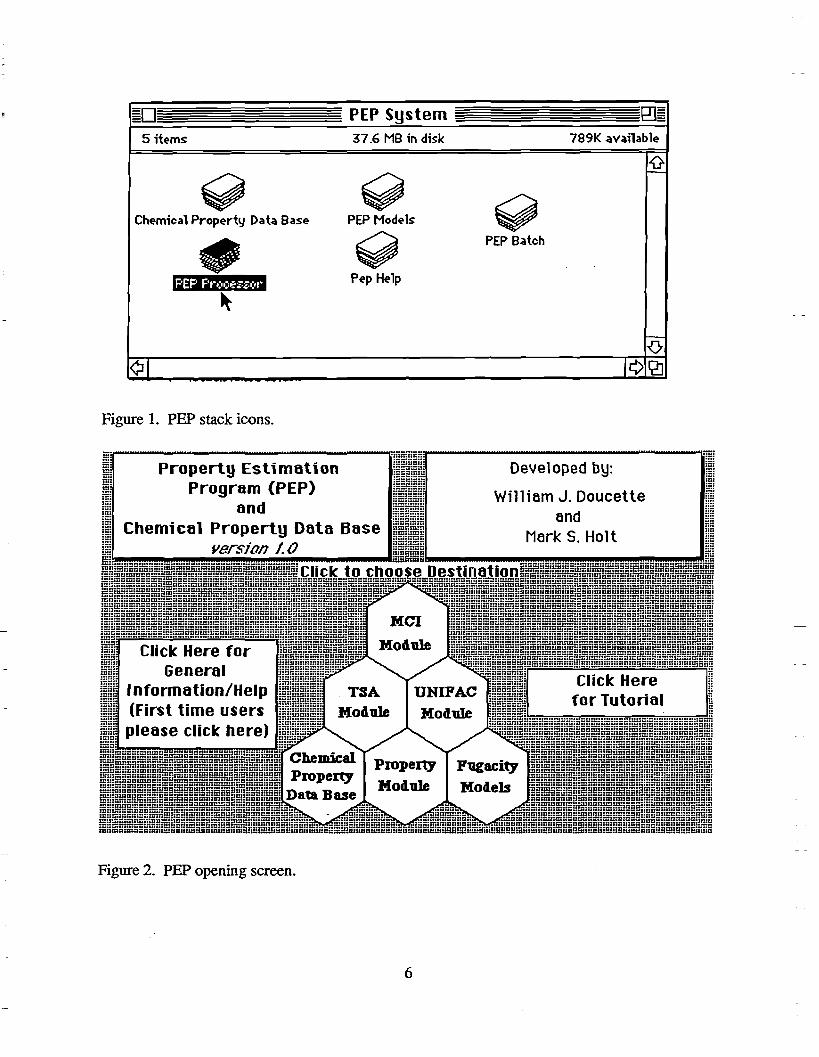
PEP is started from the Macintosh operating system by clicking twice (double clicking) on any one of the five stack icons, expect the PEP batch stack, shown in Figure 1. The five stacks must be in the same folder on a hard disk. This will open the PEP Processor stack and display the

opening card shown in Figure 2. P~ can also be used by opening any HyperCard stack and then choosing "Open" from the ''File'' menu and selecting the ''PEP Processor" stack.

5

o 5 items

~ Chemical Property Data Base

Figure 1. PEP stack icons.

Property Estimation Program (PEP)

and

PEP System 37.6 MB in disk

~ PEP Models

~ Pep Help

Chemical Property Doto Bose ver..<ljon l.lJ ____ _

General Information/Help (First time users please clicle here)

Figure 2. PEP opening screen.

6

789K available

~ PEP Batch

Developed by:

Willi em J. Doucette end

Merk S. Holt

Menus, Buttons and Icons

In Macintosh applications most cursor movements are accomplished by use of the mouse or trackball. Action buttons are operated by positioning the "hand" cursor over the button area and then depressing and releasing the mouse button. This is referred to as clicking. Popup and pull down type menus are operated by positioning the hand cursor over the button and then depressing and holding the mouse button. While holding down the mouse button move the cursor over the desired menu item and release (Note: on slower machines such as the Mac Plus, the menu selections may be slow to appear, but be patient, they will eventually show up.). Figure 3 shows the steps involved in using a menu for the selection of a command. The action of moving the mouse while holding down the mouse button is called dragging.

01 •

® ... --~ Blodegntdatlon Database

PEP TSA Module MCI Module UNlfRC Module Property Module

Opening Card Bade NeHt ' Preulous lIome

I. Menu Bar before the mouse 1s pressed 2. Menu Bar after the mouse 1s pressed

,-

3. Menu Ber efter the mouse 1s moved over the desired commend but before the mouse button 1s rele!lsed.

file

Figure 3. The steps for using a menu for command selection

Edit i5 Print Help Chemical property Database Biodegradation Database

PEP TSR Module

_~.I II

HNIfRC Module Property Module

Opening Card Back HeHt Preulous lIome

The PEP software system is comprised of five HyperCard stacks that are linked together by various menus and buttons. The pull down menus, located at the top of each card and buttons

positioned at various card locations allow the user to navigate through PEP.

The Flle and Edit menus at the top of each PEP card duplicate the general File and Edit menus in Hypercard (please refer to the Hypercard manual for complete instructions.) The Go menu allows the user to move to the either of the four property estimation modules, the chemical property database, the fugacity model or the batch mode.

7

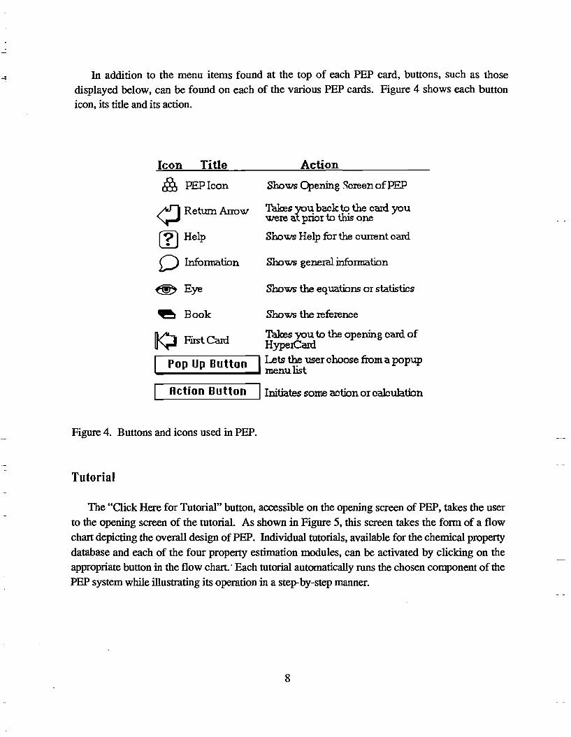
In addition to the menu items found at the top of each PEP card, buttons, such as those displayed below, can be found on each of the various PEP cards. Figure 4 shows each button

icon, its title and its action.

Icon Title

62, PEPIcon

~RetwnAnow

(?) Help

D Information

~ Eye

e Book

Action

Shows Opening Screen of PEP

'rakes you back to the card you were at prior to this one

Shows Help for the current can!

Shows general information

Shows the equations or statistics

Shows the reference

V. First Card 'Thkes you to the opening card of ~ HyperCard

I.---p-o-p-U-p-U-u-U-o-n----.I Lets ~ user choose from a popup . . menulist

L--_"_c_t_i O_"_D_u_t_t_o_"-----'1 Initiates some action or calculation

Figure 4. Buttons and icons used in PEP.

Tutorial

The "Click Here for Tutorial" button, accessible on the opening screen of PEP, takes the user

to the opening screen of the tutorial. As shown in Figure 5, this screen takes the form of a flow

chart depicting the overall design of PEP. Individual tutorials, available for the chemical property

database and each of the four property estimation modules, can be activated by clicking on the . appropriate button in the flow chart. . Each tutorial automatically runs the chosen component of the

PEP system while illustrating its operation in a step-by-step manner.

8

L ~

Done

Prope~ Property Module

Mel Module

UNIFAC Module

TSA Module,

Figure 5. Opening screen of PEP tutorial (Flow chart illustrating overall design of PEP system).

9

REFERENCE SECTION

PEP Processor

The PEP Processor stack contains the algorithms for data input, calculations and output of the physical-chemical properties estimated using MCl-Property, TSA-Property, and Property-Property correlations and UNlFAC derived activity coefficients. The PEP Processor is divided into four modules, one module for each of these estimation methods.

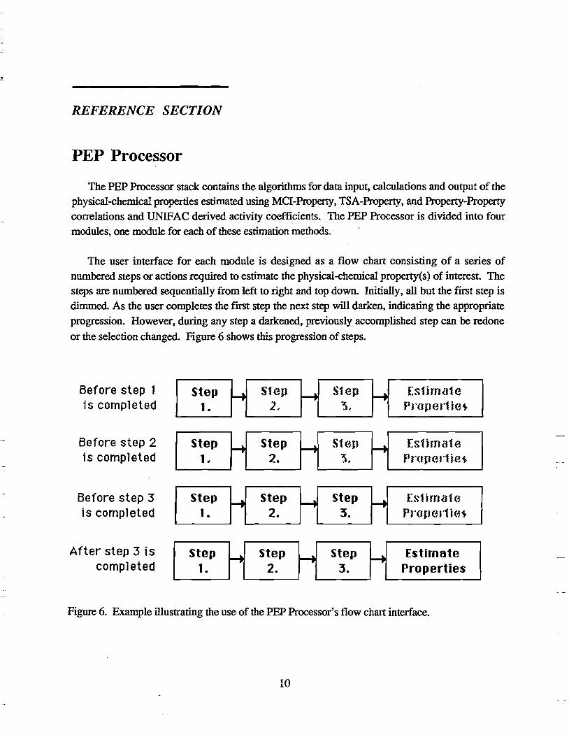
The user interface for each module is designed as a flow chart consisting of a series of numbered steps or actions required to estimate the physical-chemical property(s) of interest. The steps are numbered sequentially from left to right and top down. Initially, all but the first step is dimmed. As the user completes the first step the next step will darken, indicating the appropriate progression. However, during any step a darkened, previously accomplished step can be redone

or the selection changed. Figure 6 shows this progression of steps.

Before step 1 is completed

Before step 2 is completed

Before step 3 1S completed

After step 3 is completed

Step 1.

Step 1.

Step 1.

Step 1.

4 SteJJ ),

r-+ Step 2.

..... Step 2.

r-+ Step 2.

H St (~JJ --t [stirrwte .~, PnlJ}(~rt i(~~

--. S1<~J} 4 [stirrwt(~

'5, PnlJl(~rt ie~

H Step --t Est irrwt (~ 3. PnlJ}ert i(~~

--t Step r-t Estimate 3. Pr-oper-ties

Figure 6. Example illustrating the use of the PEP Processor's flow chart interface.

10

Mel Module

Overview

The user interface of the MCI module, like the other property estimation modules in PEP, is designed in the form of a flow chart depicting the steps that must be completed in order to use the

module. As illustrated in Figure 7 by the fully darkened Mel module card, the four steps that must

be completed before the selected physical-chemical properties can be estimated using are: (1) input the necessary structural information for the chemical of interest using either SMILES notation or a connection file, (2) calculate and display the MCls, (3) select the properties to estimate and (4)

choose the most appropriate Mel-property regression model.

PEP Processor BJ

• File Edit 60 Print Uiew 1J ~ MCI

Chemical Name: 2.2'.6.6'-tetrachlorobmhenyl SM I LES string: c u~nccccO;llc l-c2c.o:ltf;ccc_~1CU

3. Choose 4. Choose Uiew Prop. Regression PEP REF

Stats

I8Is I PCBs @~

1. Input 181 Kow I PC 6$ @~ 2oCa.c. 5. Estimate Structure ~ MCls

4 ~ Properties 181 Pu I PCBs ®~

II ~ 181" I PCBs @~

~ 181 Koc I PCBs @ ~ display MCIs

181 eCF I PCBs @ ~

. '. '. . ..... ....... . ' ........... ,. . ." ..... ' .,' ..... . .... " . ... , : ,~ •• " •• "'., .. '... "''''.. ••• •••• • > ....... ", ........ " .. " ....... , ..... , ,. "" ("""" •• " .... " •• ,', ... ,,, ..... " .. "" .. , .. " ............. ,., .. " '''''''''' .,", ... ", .. ,', ... ,", ... , ..... , .... .- • • .... N • ......... (.' U"' .. '

Figure 7. Screen display of PEP MCI module.

11

Entering Chemical Structure

Upon entering the Mel module, only the fIrst step in the flow chart is active as indicated by its darkened status. The two dimensional molecular structure of the chemical of interest is needed to calculate the MCIs. You must first input the necessary structural information using either SMllES [33,34] notation or connection files before you can continue to the second step. Select either option from the "Input Structure" popup button.

If you select SMILES, two blank: lines appear, one for the chemical name (optional) and one for the SMILES string. Once you have entered the SMILES string, click the "OK" button or the carriage return. The SMILES string must conform to the standard set by Anderson, Veith, and Weininger (1987) and Weininger (1988) with the following exceptions: a single bond connecting aromatic rings must be explicitly denoted by an "-", the SMILES string must be Hydrogen suppressed, and the SMILES string cannot contain any "{}" or "[]" qualifiers. SMILES is a chemical notation language specifIcally designed for computer use. It is a method of "unfolding" a

2D chemical structure into a single line of characters containing the structural information. For

users unfamiliar with SMILES notation, a detailed description describing its use can be found in scrollable window directly below the SMILES string input line.

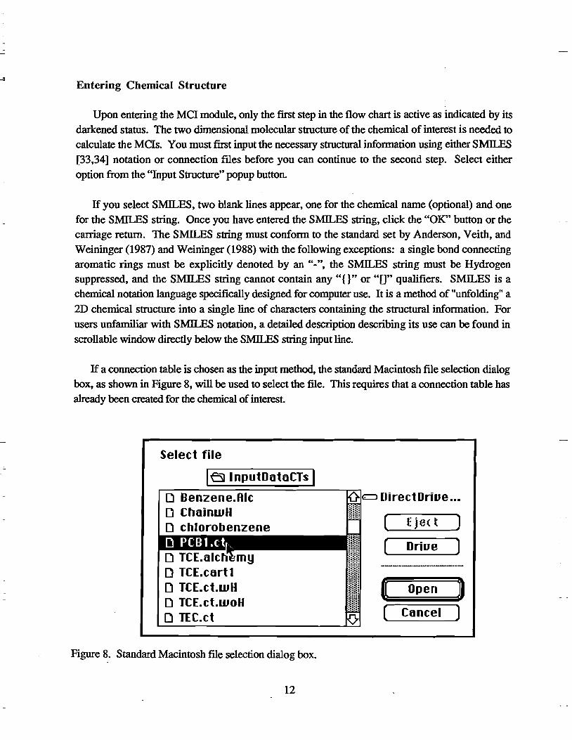
If a connection table is chosen as the input method, the standard Macintosh file selection dialog box, as shown in Figure 8, will be used to select the file. This requires that a connection table has already been created for the chemical of interest

Select file

Ie InputDataCTs I Benzene.Rlc ChainwH

[) TCE-alch my [) TCE.cart t [) TCE.ct.wH [) TCE.ct.woH [) TEC.ct

Figure K Standard Macintosh file selection dialog box.

12

lIirecUlriue •••

( t:j(Ht ]

( Driue ]

€ open» ( Cancel]

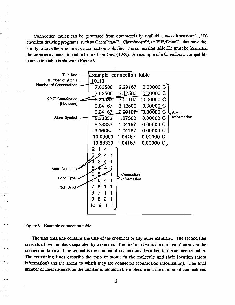
Connection tables can be generated from commercially available, two-dimensional (2D) chemical drawing programs, such as ChemDraw™, Chemintosh™, or ISIS/Draw™, that have the ability to save the structure as a connection table file. The connection table fIle must be fonnatted the same as a connection table from ChemDraw (1989). An example of a ChemDraw compatible connection table is shown in Figure 9.

Title line connection table Number of Atoms

Number of Connnections

x, Y,Z Coordinates (Not used)

Atom Symbol

Atom Numbers

80ndType

Not Used

9.04167 9.04167

.33333 8.33333 9.16667

10.00000 10.83333 2 1 4 1 3 1

1 6 1 1 7 1 1

9 8 2 1 10 9 1 1

Figure 9. Example connection table.

2.29167 3.12500

. 4167 3.12500

1.87500 1.04167 1.04167 1.04167 1.04167

Connection Information

0.00000 C o. 000 C

·0.00000 C 0.00000 C

. 0000 C 0.00000 C 0.00000 C 0.00000 C 0.00000 C 0.00000 C

Atom Information

The first data line contains the title of the chemical or any other identifier. The second line consists of two numbers separated by a comma. The first number is the number of atoms in the connection table and the second is the number of connections described in the connection table. The remaining lines describe the type of atoms in the molecule and their location (atom information) and the atoms to which they are connected (connection information). The total number of lines depends on the number of atoms in the molecule and the number of connections.

13

Atom infonnation is contained in four columns separated by one or more spaces. Columns one through three are the X, Y ,Z coordinates of the atom (not used for calculation of MCls) and column four contains the atom symbol (e.g. C, CI, Br, N etc.). Connection infonnation is contained in four columns of whole numbers. Columns one and two contain the atom numbers of the atoms that are connected (atoms are numbered consecutively), column three contains the bond type (1, 2,

3, or 4), and column four usually contains a 1 (not used). The bond type in column three can be either "1" for a single bond, "2" for a double bond, "3" for a triple bond, or '~4" for an aromatic bond. (NOTE: The Macintosh compatible molecular modeling program, Alchemy 1ITM, generates

files containing connection table information along with 3D atomic coordinates. To use alchemy

files for input into the MCI module simply treat the alchemy file as a "ChemDraw Connection Table" .)

As described in the next section, MCls are calculated from the hydrogen suppressed structure

of a chemical. Consequently, for the most efficient calculation of MCI, the connection tables created for input into the MCI module should be created from hydrogen suppressed structures. If the connection tables are not hydrogen suppressed PEP will automatically remove them. This can result in a significant increase in the time required to calculate the MCls.

Calculating MCIs

As soon as the structure is entered, the second step becomes active. Clicking on the "Calc.

MCls" button starts the calculation of the MCIs. If the structure was entered as a SMILES string the "mciSmile" XFCN converts the SMILES string into the proper format for the "mcichi" XFCN

which calculates the MCls. Similarly, if a connection table was used for input the "mciConvert"

XFCN converts the connection table into the proper fonnat. The MCIs that are calculated are listed along with the variable names in Table 1. Once the MCls have been calculated, they can be viewed, exported, or printed by using the "Display MCIs" button under the "Calc. MCls" button.

14

Table 1. MCIs calculated by PEP.

Variable Name

np nel nch npe bp bel beh bpc vp vel vch vpc .6.vp

How PEP calculates MCIs

MCITitle

normal path normal cluster normal chain normal path/cluster bond path bond cluster bond chain bond path/cluster valence path valence cluster valence chain valence path/cluster delta valence path

Orders calculated

o through 6 3 through 6 3 through 6 4 through 6 o through 6 3 through 6 3 through 6 4 through 6 o through 6 3 through 6 3 through 6 4 through 6 o through 6

To calculate the MCIs for a given compound, a delta (d) value are fIrst assigned to each non­

hydrogen atom in the structure. Three d values were computed in this study: normal, bond, and

valence. Normal deltas are computed by summing the number of bonds (single, double, etc. are counted as one bond) connected to the atom whose delta is being calculated. The bond deltas are

calculated the same as the normal deltas except the bonds were taken at their face value (single is

one, double is two, etc.) instead of each bond being equal to one. Valence deltas for each atom are

computed according to equations (1) and (2) (Kier and Hall, 1986):

dv=Zv- h

dv = (Zv - h)/(z - Zv)

(1)

(2)

where dv is the valence delta, Zv is the number of valence electrons in the atom, h is the number of

hydrogen atoms bound to the atom, and Z is the atomic number of the atom. Equation (1) is used

for those atoms in the first row of the periodic chart, and equation (2) is used for all other atoms.

Once the delta values have been calculated for each atom in the molecule. simple, bond and valence indices of different orders and types can be calculated. The order refers to the number of

bonds in the skeletal substructure of fragment used in computing the index: zero order defInes

individual atoms, first order used individual bond lengths, second order uses two adjacent bond combinations, and so on. The type refers to the structural fragment (path, cluster, path/cluster or

15

chain) used in computing the index. A more detailed explanation of the calculation of MCls can be found in Kier and Hall (1986).

The MCI calculation routine in PEP calculates simple, bond and valence indices of several types (path, cluster, chain, and path/cluster) and orders (0 through 6), if possible, for each molecule, resulting in a maximum of 54 index values for each molecule.

To account for non-dispersive force effects on aqueous solubility and solubility related

properties zero through six order Il valence path indices (IlX), as described by Bahnick and Doucette (1988), are calculated by PEP, in addition to the 54 indices described above. To calculate

IlX indices, a nonpolar equivalent is made by substituting C for 0 or N atoms. MCls are calculated for the nonpolar equivalent and values for Ilc can be computed for each type of index by:

IlX = (X)np - X (3)

where IlX is the delta index, (x)np is the index for the non-polar molecule and X is the index for the

original molecule.

Choosing the Properties

Mter the MCls have been calculated, the third step becomes active. Select the property or properties you would like to estimate by clicking on the check box button next to it You can simultaneously select all the properties by holding down the shift key and clicking anyone of the

property buttons.

Choosing the Regression Models and Chemical Classes

Mter the properties are selected, step four becomes active and the regression models available for each property are displayed in a popup menu. Two categories of MCI-property relationships

are displayed for each property. The first category of MCis property relationships, preceded with the word PEP, were developed in this project using the experimental values reported in the PEP

property database. ''Universal'' MCI-property relationships were developed using all available

experimental data for a given property regardless of chemical class. "Class-specific" MCI-property relationships were developed if property values were available for a sufficient number (10 or greater) of compounds within a particular chemical class (i.e. PCBs, PABs, ureas). In addition, several multi-class MCI-property correlations were developed for more broad classes of compounds such as: halogenated aliphatics and halogenated aromatics.

16

The second category of MCI-property relationships displayed for each property were obtained

directly from the literature and are located below the PEP relationships, separated by a gray line, in the popup menu. By clicking the "book" found at the left of each literature MCI-property

regression model, the coefficients, r2 value and the appropriate citation can be can be displayed

To illustrate the potential hierarchy of MCI-property relationships available to the user, an

example for the predicting the vapor pressure (Pv) of a polychlorinated biphenyl (PCB) is provided

below. The are three appropriate PEP-derived MCI-property relationships available to the user,

one developed using only PCBs, one using halogenated aromatics including PCBs and one using all compound types:

log Pv = 5.814 (nc5) - 2.428 (np3) + 9.479

log Pv = -1.559 (bpI) + 6.622

log Pv = -1.275 (np3) +5.261

(PCBs)

(Halogenated aromatics)

(Universal)

Generally, the use of a "class-specific" relationship, if available, should provide the best

estimate (Le. the estimate associated with the least amount of uncertainty). To automatically aid you in choosing the most appropriate MCI-property relationships, PEP looks in the SMILES string

or connection file for groups of atoms and bonds that distinguish various chemical classes. The

number of MCI-property relationships or chemical classes that are chosen by the program is

determined by the number of different distinguishing subgroups that are found. For the example

shown above, the most appropriate regression model, PCBs, would be made the default equation.

The two other appropriate models, halogenated aromatics and Universal, would be denoted with a

• in the popup menu. If the compound entered into PEP does not fit one of the class specific models the "Universal" equation is selected as the default. You may also choose to ignore the

regression model chosen by PEP and select your own.

MCI-property regression models are available for the following "classes" of chemicals:

Universal, Universal Nonionizable, Universal Ionizable, Alcohols, Anilines, Carbamates,

Halogenated, Aliphatics, Nonhalogenated Aliphatics, Halogenated Aromatics, PCBs, PAHs,

Phenols, Triazines, and Urease Examples of representative chemicals for each of the classes can

be found in the View menu. To see the structures of the chemicals click on the class name. Not all of the classes listed above are implemented for each property. The models not available for the

properties to be estimated are dimmed in the popup menu.

17

Statistics Cards

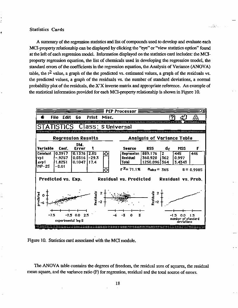
A summary of the regression statistics and list of compounds used to develop and evaluate each

MCl-property relationship can be displayed by clicking the "eye" or "view statistics option" found at the left of each regression model. Information displayed on the statistics card includes: the MCl­

property regression equation, the list of chemicals used in developing the regression model, the

standard errors of the coefficients in the regression equation, the Analysis of Variance (ANOV A)

table, the r2 value, a graph of the the predicted vs. estimated values, a graph of the residuals vs.

the predicted values, a graph of the residuals vs. the number of standard deviations, a nonnal

probability plot of the residuals, the X'X inverse matrix and appropriate reference. An example of

the statistical infonnation provided for each MCl-property relationship is shown in Figure 10.

PEP Processor 0 a File Edit 60 Print Misc. (?) ~ ~.

STATISTICS Class: S Universal

Regression Results Analysis of Variance Table

std. Variable Coef. Error t Source RSS df MSS F Constant 0.3917 0.1376 2.85 Q Reg renion 889.176 2 445 446 vp1 -.9257 0.0316 -29.3 Residual 360.920 362 0.997 Avp1 1.8251 0.1047 17.4 Total 1250.096 364 3.4343 MP-25 -0.01 10 r2= 71.1" nobs= 365 s= 0.9985

Predicted YS. Exp. Residual YS. Predicted Residual YS. Probe

~ . tl ~ ... , ~ . 11\ 2 . . ~ 0 . •• ~ .:~':. .. ~.::~~ :::7 J:!: •• I' .41: • ~ .• !~lTc':." ~~ "5 -2 • "lo~ ':. .. ~,,~:. . L -6 ..• ~ . Q. • .'~ •• IX: IX: .'

f f I f I I I I I I I f -7.5 -2.5 0.0 2.5 ". -6 -3 0 3 -1.5 0.0 1.5

experimt'Otallog S number of standard deviations

...... :.:.:.~ ..... ::.:.:~ ......... : ....... :: :.~~ .... : ~~ ......... ~ .. ~.: ~:.; ~ ...... ':':.: ... ~~: .. "~"""~,~ ....... ~~~~ .... ~'t:~:-.~ .. ",,:~~ .... ~ .:~:: ...... ~: w ... ~~~\~:~.~ ,:~' ~~ .:: l~~:::.~~:: .. ~: .. '~t~~ .. ~ .. ~:; :.~: ....... : ~\\\\.::.:: :.: .. :.\ : .. ~\ .... ;.~~~:: :~; ...... ° ~.~~m~.: ... ; \. ~ .... ;0:

Figure 10. Statistics card associated with the MCI module.

The ANOV A table contains the degrees of freedom. the residual sum of squares, the residual mean square, and the variance ratio (F) for regression, residual and the total source of errors.

18

l -'

The X'X inverse matrix is used in PEP to calculate the prediction interval of an estimate. The matrix is derived by pre-multiplying the X matrix by its transpose and then inverting the result. The X matrix has a column for each variable in the regression equation and a row for each obselVation used to calculate the regression equation. Each row contains the value used for each of the variables in the regression equation. For example, if the regression equation is

Yj= bO + blXjl + b2Xj2

where j is 1 to the number of obselVations, Yj is the estimated values for each obselVation, the bi are the regression coefficients, and the Xji are the values of the variables used then the X matrix is

1 XlI X12 1 X21 x22

1 Xjl Xj2.

The resulting X'X inverse is a square matrix with the number of rows and columns equal to the number of variables in the regression equations.

If the QSPR or QPPR was taken from the literature only the input variables and the statistical information provided in the original reference is included.

Estimating the Properties and Viewing the Results

Click the "Est. Property" button to calculate the selected properties. The results card displays the estimated properties and their respective 95% prediction interval Note: 95% prediction intervals are not available for Mel-property relationships taking from the literature. You can return to the previous card. by clicking on the ''return'' button at the upper right corner of the results

card. The "Go" menu can be used to move to another module. You can compare the estimate property values with those contained in the "Chemical Property Database", if available, by clicking on the "Look in DB" button. Clicking this button activates a database "search by name" routine. The name on the results card. must match exactly the name in the database for the search routine to

find the compound. If a property vaiue is not found an NA will be displayed.

Adding or Deleting Mel-Property Regression Models

Additional MCI-property regression models can be added to the PEP MCI module through the statistics ~ards. Choosing the "New Stat. Card" option from the "Misc." menu of a statistics cards

19

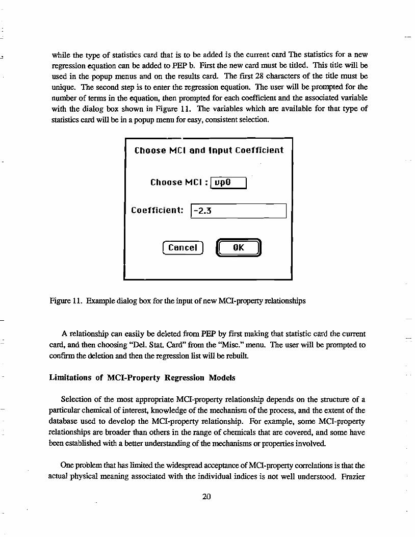
while the type of statistics card that is to be added is the current card The statistics for a new regression equation can be added to PEP b. First the new card must be titled. This title will be used in the popup menus and on the results card. The first 28 characters of the title must be

unique. The second step is to enter the regression equation. The user will be prompted for the number of terms in the equation, then prompted for each coefficient and the associated variable with the dialog box shown in Figure 11. The variables which are available for that type of statistics card will be in a popup menu for easy, consistent selection.

Choose Mel and Input Coefficient

Choose MCI : I upO

Co e ffici en t: .... 1-_2_._3 ______ -----'

( Concel) € OK D

Figure 11. Example dialog box for the input of new Mel-property relationships

A relationship can easily be deleted from PEP by first making that statistic card the current

card, and then choosing "Del. Stat. Card" from the "Misc." menu. The user will be prompted to

confirm the deletion and then the regression list will be rebuilt.

Limitations of Mel.Property Regression Models

Selection of the most appropriate Mel-property relationship depends on the structure of a particular chemical of interest, knowledge of the mechanism of the process, and the extent of the database used to develop the Mel-property relationship. For example, some Mel-property

relationships are broader than others in the range of chemicals that are covered, and some have

been established with a better understanding of the mechanisms or properties involved.

One problem that has limited the widespread acceptance of MCI-property correlations is that the

actual physical meaning associated with the individual indices is not well understood. Frazier

20

(1990) and Doucette and Holt (1991), however, have shown a strong correlation between calculated molecular surface area and several MCIs for a variety of organic chemicals. MCI­property correlations tend to be class specific and thus are highly dependent on the type and range of compounds that were used to derive a particular correlation. Indiscriminate use of such models without an examination of number and type of compounds used to develop the model can result in considerable error.

21

TSA Module

Overview

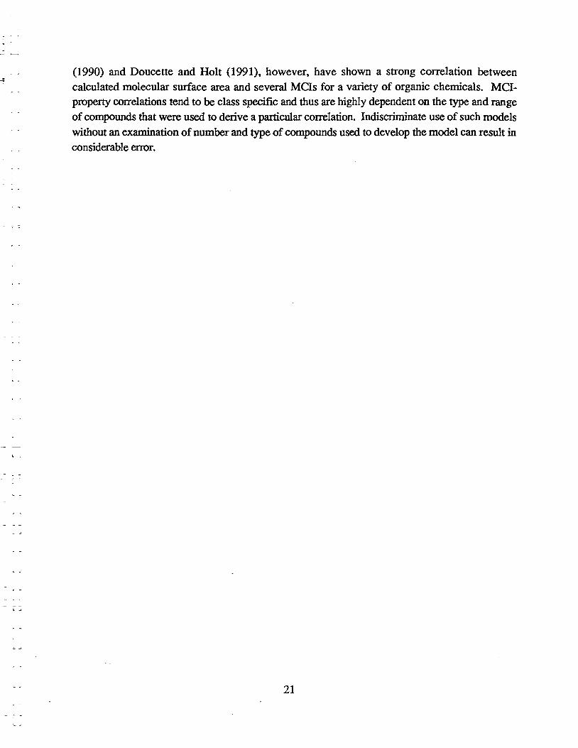
As shown in Figure 12, the TSA module is similar in design to the MCI module. However, unlike molecular connectivity, the calculation of TSA requires infonnation describing the geometry

of the molecule in terms of its 3-D atomic coordinates.

PEP Processor F!I§I C File Edit 60 Print Uiew (1) ~

TSA Chemical Name:.1.,.~:J.6,6·-telr.~chlor~t~J.Dheny~

SM I LES String: -_.- ......... _ ....... . - _ ..... .... _ ... . ...

3. Choose 4. Choose Uiew Prop. Regression PEP REF

Stats

rgjS l PCBs I~~

181 Kow

I PCBs :~~ .. 5. Estimate 1. Input ~ 2. calc.

~ Structure TSRs [81 Pu PCBs ~~ -;t~erties

jf jf [81" j HalQgenated Aromatics I~~

Edit Y~A @ [81 Koc I Halogenated Aromatics I@~ der Ynls

R~dii disp latl TS As [81 BCF I Universal ~~~

~~i::::!:::: ,~w •• ,. ~ .w. :'0;':: :~~ •••• ,."".. .. ~ u. ,~~,::~;: :~~.:"~,w;..;,,.;.w;.:.m~i.;.:J~:~,(~~,~: MV," ..... , ,,,:: :::: ;:; .:.w.·, .w •• ~ ....... : u;.; ... ;~.::. "~w ................... >;~....:~~;!: :~~~~~'NNN'" m;''':v~:~~:::. :..mN .............. '''u~,: ~L::,::~ ~~, ~ ... ,' a

Figure 12. TSA module card from PEP

TIrree-dimensional coordinates· can be obtained from X-ray crystallography data or from molecular modeling. Alchemy from Tripos Associates (1989) and Chem3D+from Cambridge Scientific (1989) are examples of Macintosh compatible molecular modeling software that allows the user to draw a chemical structure, energy minimize the structure, and produce a file containing the three-dimensional coordinates. The TSA module is also designed to accept files generated by

other h~dware/software combinations including UNIX or V AX versions of CONCORD {Tripos

22

li... .:...

Associates, Inc., 1990), a hybrid expert system and molecular modeling software designed for the rapid generation of high quality approximate 3-D molecular structures.

Entering the Structural Information

To estimate properties using the TSA module, you must fust input the necessary structural

information by using one of the three options available under the popup menu titled "Input

Structure": (1) Alchemy fIle, (2) cartesian coordinates file, or (3) manually entered c~rtesian

coordinates. The preferred method of structural input is via Alchemy files because they contain

both the three-dimensional structure and the connection information. This infOImation allows PEP

to calculate the chemical's TSA and determine the most appropriate TSA-property relationship based on chemical class. Therefore, if an Alchemy fIle is chosen for the input then only the file

selection dialog box will be presented for selection of the file. However, if ether of the cartesian

coordinate options are selected for input, both the standard file selection dialog box will be

presented and an opportunity to select the connection table file or enter a SMILES string will be

presented.

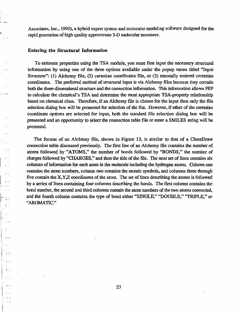
The format of an Alchemy file, shown in Figure 13, is similar to that of a ChernDraw

connection table discussed previously. The fust line of an Alchemy file contains the number of

atoms followed by "ATOMS," the number of bonds followed by "BONDS," the number of

charges followed by "CHARGES," and then the title of the file. The next set of lines contains six

columns of information for each atom in the molecule including the hydrogen atoms. Column one

contains the atom numbers, column two contains the atomic symbols, and columns three through five contain the X, Y ;Z coordinates of the atom. The set of lines describing the atoms is followed

by a series of lines containing four columns describing the bonds. The first column contains the

bond number, the second and third columns contain the atom numbers of the two atoms connected,

and the fourth column contains the type of bond either "SINGLE," ''DOUBLE,'' "TRIPLE," or "AROMATIC."

23

Number

of Atoms

Number

of Bonds

6 ATOMS, 5 BONDS, not used title

0.0008 0.0149 o CHARGES, TCE 0.0048 0.0000

X,Y,Z coordinate

Bond ty 3 3

Figure 13. Example Alchemy file.

1.0242 0.0245

Connection

Information

0.0000 0.0000 0.0000

Atom

Information

PEP accepts cartesian coordinates files having the following format The file has one header

line indicating the number of atoms in the molecule. The rest of the lines in the file describe each

atom in the molecule. Only the first five columns of each line are used. Column one contains the atom symbols, column two contains the atom numbers, and columns two through five contain the

X, Y;Z coordinates of the atom. An example cartesian coordinates file is shown in Figure 14.

Number Atom Atom of Atoms Symbols Numbers X Y Z coordinates Not used

1.658981 1.41 048 0.220383 12 2 2 0.678864 0.010635 0.004303 2 1 3 0.661346 0.015198 0.109131 2 2 4 1.498978 1.476791 0.333939 12 3 5 1.607437 1.456451 0.031769 12 3 6 1.277542 0.912277 0.055084 5 2

Figure 14. Example Cartesian coordinate file.

24

If the option to manually enter the coordinates is chosen then a card is presented, as shown in Figure 14, that allows the coordinates and atom symbol of each atom to be entered individually from the keyboard. The X,Y,Z, coordinate values and atom symbols for each atom in the molecule are entered in the appropriate labeled boxes one at a time. After the information for each

line is correctly entered the "Line OK" button is clicked. This enters the information into the scrollable window below. This process is repeated for each atom in the molecule. When all the

atoms have been entered clicking the ''Done'' button will send the structural information to the TSA module.

a File Edit Go Print Misc.

Enter XYZ coordinates for the chemical Chemical Name:JJen~.~lJe . ___ _

Fill in one atom at a time at the bottom, type Return or Tab to put it into the table. To Edit an entry clicle on the line in the table. Click "nil Done· when the table is complete.

X coord Y coord Z coord Atom Symbol

1'--2_ ....... I'--c __ --'-___________ '----_---o1 ¢ Line OK D 1 C 1 1 1 ~

( Clear)

( cancel)

( nil Done)

. :': :.:::' ", .': ... ,. ".:'" .. ::' . '::: .. '.,: ::' :' ... :... . ::' ':" ...... : ........... : .. ': ............. ':::: ::'.: ": . ::: . ::" :':: .... :: .': ... : .. ,:'::' . '::. "::', : .... :: ... ',::":: .. : :'::":'

Figure 15. Example card for the entty of atomic coordinates.

Calculating Total Surface Area (TSA)

In addition to the 3-D molecular structure, the user must also input van der Waals radii for each

of the atoms before the TSA of the molecule can be calculated. PEP automatically enters a van der

Waals radius for each atom using values from Pauling (1960). However, when the "Calc. TSA" button is clicked the user has the opportunity to edit the van der Waals radii using the dialog box shown in Figure 16.

25

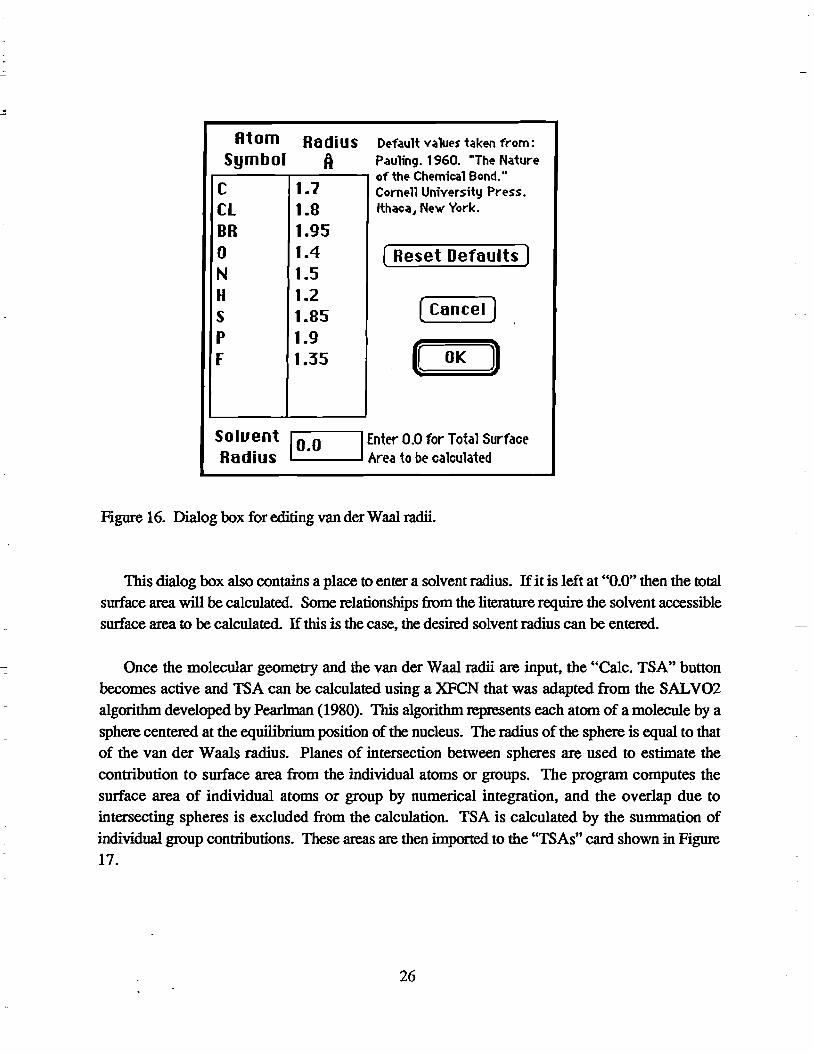
fltom Radius Default values taken from: Symbol ft Pauling. 1960. "The Nature

ofthe Chemical Bond." C 1.7 Cornell University Press. Cl 1.8 Ithaca I New York.

DR 1.95 0 1.4 ( Reset Defaults) N 1.5 H 1.2 S 1.85 ( Cancel )

p 1.9

K » F 1.35 OK

Soluent 10•0 1 Enter 0.0 for Total Surface

Radius Area to be calculated

Figure 16. Dialog box for editing van der Waal radii.

This dialog box also contains a place to enter a solvent radius. If it is left at "0.0" then the total

surface area will be calculated. Some relationships from the literature require the solvent accessible

surface area to be calculated. If this is the case, the desired solvent radius can be entered.

Once the molecular geometry and the van der Waal radii are input, the "Calc. TSA" button becomes active and TSA can be calculated using a XFCN that was adapted from the SALV02

algorithm developed by Pearlman (1980). This algorithm represents each atom of a molecule by a

sphere centered at the equilibrium position of the nucleus. The radius of the sphere is equal to that of the van der Waals radius. Planes of intersection between spheres are used to estimate the

contribution to surface area from the individual atoms or groups. The program computes the

surface area of individual atoms or group by numerical integration, and the overlap due to

intersecting spheres is excluded from the calculation. TSA is calculated by the summation of

individual group contributions. These areas are then imported to the "TSAs" card shown in Figure 17.

26

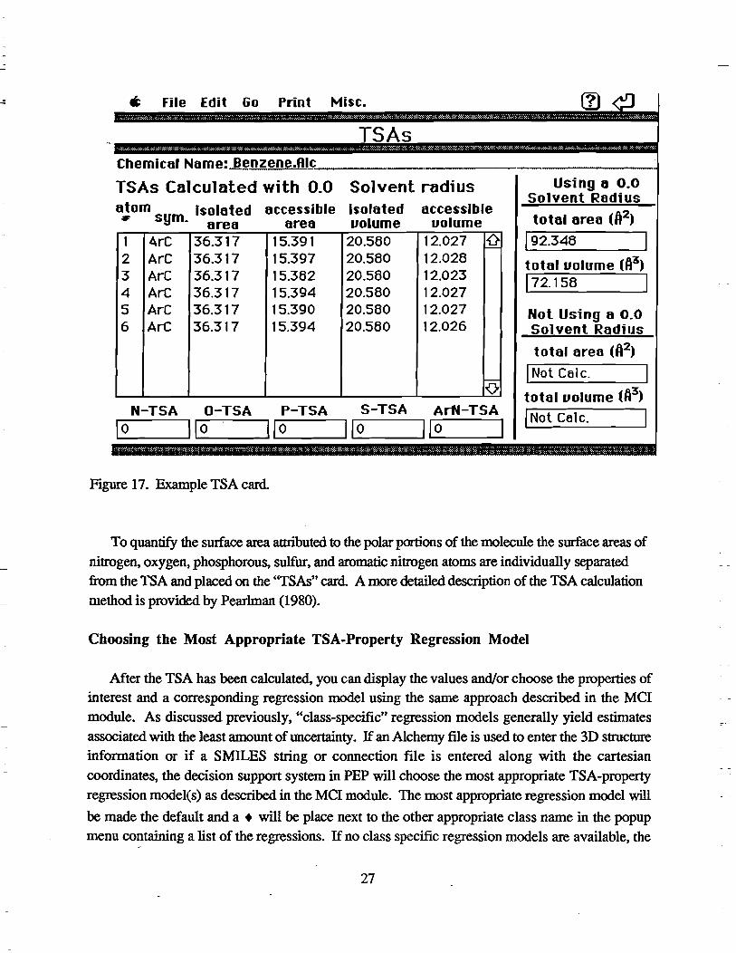
a File Edit Go Print Misc.

TSAs .~... . ~~,,"""' .. ::" ••. , ....... ; .... .: . ..: ....... ;... ..... ;. ................ , ........ , .: ............ y-:,.: ..... " .. :.; .. ; .... :. ........ : ... ,: .......... ;.:.;;..,;. ..... ; .. · .... u •• ~.:. .......... :;. ... :.: .....•• ' ................... ;..,;.. ........... " ..... .;.

Chemica' Name:J!~nz.!!~1JJj::..-_________ _

TSAs Calculated with 0.0 Solvent radius atom isolated accessible Isolated accessible

# sym. area area vo.ume volume 1 4rC 36.317 15.391 20.580 12.027 ~ 2 ArC 36.317 15.397 20.580 12.028 3 ArC 36.317 15.382 20.580 12.023 4 ArC 36.317 15.394 20.580 12.027 5 ArC 36.317 15.390 20.580 12.027 6 ArC 36.317 15.394 20.580 12.026

0 N-TSA O-TSA P-TSA S-TSA ArN-TSA

11...-0 __ ---111 I...-o __ --IIIL-0 __ --Il 1...-10 __ --111 0 1

Using 8 0.0 Solvent Radius

tota. area (A2)

192.348

total volume (A3)

172.158 1

Not Using a 0.0 Solvent Radius

total area (ft2)

1 Not Calc.

total volume (ft3)

I Not Calc.

":'" . "': ',:' ............... : ," ....... ," ," ..... ::: .. :", ": ........ ,. :':." .. " .. ," .... "':',::.:'" ......... ",: .. :":':: ....... : ...... :. ", ...... : ...... ' .. :' .... :',: ." ...... "'::' .:':' :',' :'." .

Figure 17. Example TSA card

To quantify the surface area attributed to the polar portions of the molecule the swface areas of

nitrogen, oxygen, phosphorous, sulfur, and aromatic nitrogen atoms are individually separated

from the TSA and placed on the ''TSAs'' card. A more detailed description of the TSA calculation

method is provided by Pearlman (1980).

Choosing the Most Appropriate TSA.Property Regression Model

After the TSA has been calculated, you can display the values and/or choose the properties of

interest and a corresponding regression model using the same approach described in the MCI

module. As discussed previously, "class-specific" regression models generally yield estimates

associated with the least amount of uncertainty. If an Alchemy file is used to enter the 3D structure

information or if a SMll..ES string or connection file is entered along with the cartesian

coordinates, the decision support system in PEP will choose the most appropriate TSA-property

regression model(s) as described in the MCI module. The most appropriate regression model will

be made the default and a + will be place next to the other appropriate class name in the popup

menu containing a list of the regressions. If no class specific regression models are available, the

27

, -

. -

, -

"Universal" equation will be made the default. The operation of the TSA module from this point on is identical to that of the MCI module. Note: for solid solutes the melting point is needed to estimate the solubility. When the "S" button is click~ the user is prompted with a dialog box to enter the melting point. Because the solubility will be estimated at 250 C, only if the melting point is above 250 C (solid solute) will the value be required. If the melting point is below 250 C it is set equal to 250 C. At this time only the "s 250 C' and "known" options are useable in the dialog box.

TSA-property regression models available within PEP are: Universal, Universal Nonionizable, Universal Ionizable, Alcohols, Anilines, Carbamates halogenated Aliphatics, Nonhalogenated

Aliphatic, Halogenate Aromatics, Nonhalogenated Aliphatic, Halogenate Aromatics, PCBs, PARs, Phenols, Triazine, and Ureas. Not all models are available for' each property. The models not available for the properties to be estimated are dimmed in the popup menu. You can also view the

statistical information associated with each model by clicking on the "eye" next to the regression

equation.

Estimating the Properties

Mter the appropriate TSA-property relationships have been selected you can now click on the ''Estimate Property" button to calculate the estimated properties. The estimated properties and their

respective 95% prediction interval will be displayed on the results card. Return from the results card by clicking on the "Return arrow" button at the upper right hand corner of the results card.

Use the "Go" menu to move to another module. View values in the Chemical Property Database by clicking on the ''Look in DB" button. If a property value is not available in the database, an NA will be displayed in the property field.

Development of TSA.Property Relationships

The PEP TSA-Property relationships that were were developed using stepwise regression

techniques and the data in the Chemical Physical Data Base. The stepwise regression was stopped when the coefficient of determination did not improve by at least 0.05 when the next variable was added.

For compounds containing polar functional groups, the addition partial TSA terms (Le. nitrogen (N-TSA), oxygen (O-TSA), aromatic nitrogen (ArN-TSA), sulfur (S-TSA), or

phosphorous (P-TSA» significantly improved the TSA-property regression models. To view the

regression information by clicking on the "eye" next to the regression title on the results card or on the TSA card.

28

r -

r -

Limitations of TSA-Property Relationships

A major factor in the solubilitzation process is the energy required to create a cavity in the solvent into which the solute is placed. The energy needed for the hole formation is considered to be proportional to the surface area of the solute. TSA has been found to be linearly related to the logarithm of solubility for many classes of non-ionizable organic chemicals.

As with the Mer module, selection of the most appropriate TSA-property relationship depends on the structure of a particular chemical of interest, knowledge of the mechanisI!l of the process, and the extent of the database used to develop the TSA-property relationship. Some TSA-property relationships are broader than others in the range of chemicals that are covered and some have been established with a better understanding of the mechanisms or properties involved.

29

UNIFAC Module

Overview

The UNIFAC (UNlQUAC Functional Group Activity Coefficient) group contribution method for calculating activity coefficients, as described by Grain (1990), is implemented using both HyperTalk and an XFCN. The functional group interaction parameters, presented by Gmehling et ale (1982) and derived from vapor-liquid equilibria (VLE), are used in the calculation routine but can be changed by the user. Mter the activity coefficients are calculated they can be displayed

along with relevant intermediate values and used to estimate S and Kow by the following

expressions (Arbuckle, 1986):

Kow = 0.115 yoow /yooo

S (moI/L) = 55.6 / yoow

(2)

(3)

where l°ow is the activity coefficient of the chemical infinitely dilute in water and "too is the

activity coefficient of the chemical infinitely dilute in octanol.

The operation of the UNIFAC module, illustrated in Figure 18, is considerably different than the correlation modules previously described. To use the UNIFAC module the you must input structural information, calculate the activity coefficients, choose then choose the properties to be estimated. Currently the only properties that can be directly estimated using the UNIFAC module

are S and Kow.

30

, -

l "

PEP Processor IF.!!

C File Edit Go Print Uiew l1J ~

UNIFAC , , ' . ~ ':'- ••• ~ "~, ~~ ... ,.;,,; ,,',:.; , .. ,: '" , ...... :", ~';'Vv .............. ' " " ... ,' .. , ... ": , ,. '" .... u} "~ •• ~

Chemical Name: 2.2',6.6'-tetrochlorobiDhenul SMILES String: cl (COccq(j:Ocl-c2c(Cllcccc2(Cn

UNIFAC Groups: 4 ACC1 6 ACH 2 AC

3, Choose Property

I. Input 2. calculate I8IS ~. 4. Estimate

Structure ~ RctiUity ----I r----- Prop~ Coefficients 1:81 Kow ~

Edit UNlfAC ~ Permeters I>isp 1~ ",ct. Coeff.

. .. .. '~' .. ~ "':., ..... ,': """''''''''''''':u " .. " .. ~ ........ ' ~ . .

. ~. . .. ,. ,,, .. : " : .. ' ...... ,. U"'. ,. : .... • 'N"" .. n ..... n .. •

Figure 18. Example card from the PEP UNIFAC module.

Entering Structural Information

Calculation of activity coefficients via the UNIFAC approach requires that the user input the

valid UNIFAC groups that make up the chemical of interest and the number of each group present

PEP provides the user with three options for entering the appropriate UNIFAC groups using the popup menu under the button titled "Input Structure": (1) hand selecting the groups from a list in HypeICanL (2) using a connection table, and (3) using SMILES.

H the connection table option is chosen, a the standard flle selection dialog box is presented

where the user can select the desired connection table flle. The tlStructtl XFCN then uses the

connection information to dissect the molecule into its UNIF AC groups.

H SMILES is chosen as the input method, the user is then prompted to input the chemical name

and the SMILES string. The Struct XFCN uses the connection information contained in the SMILES string to build the UNIFAC input string.

31

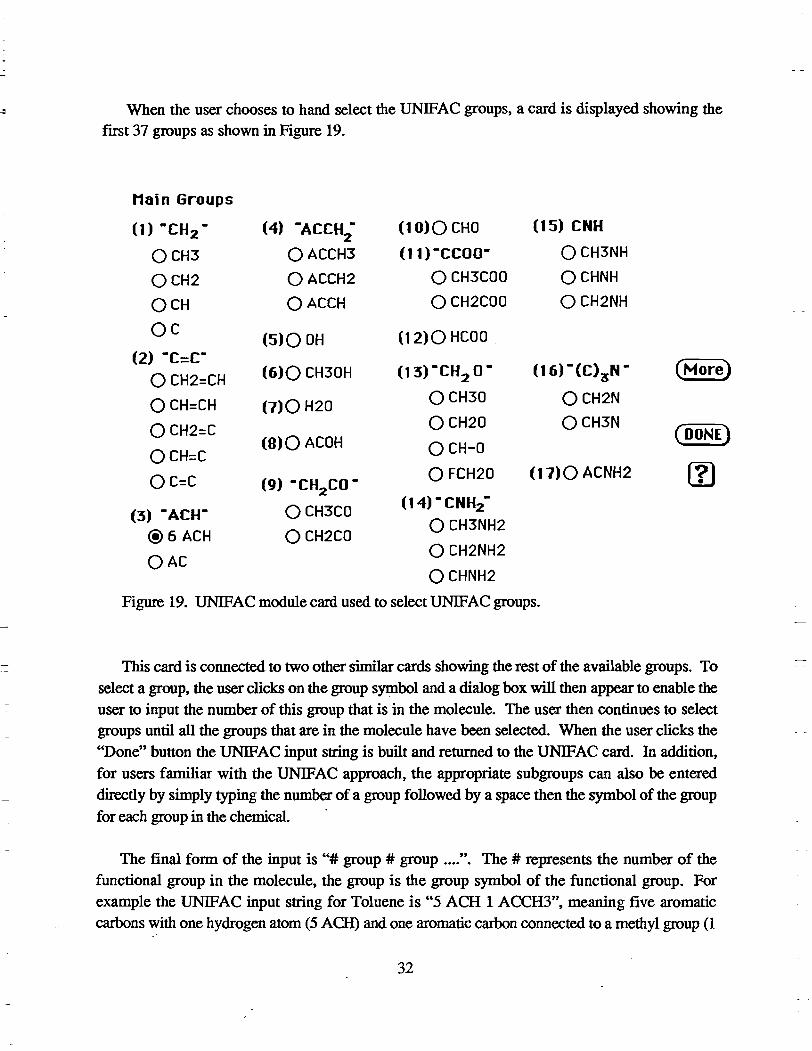
When the user chooses to hand select the UNIFAC groups, a card is displayed showing the first 37 groups as shown in Figure 19.

Main Groups

(0 -CH2 - (4) -ACCH-2

(10)0 CHO (15) CNH

OCH3 o ACCH3 (11) -CCOO- o CH3NH

OCH2 o ACCH2 o CH3COO OCHNH

OCH o ACCH o CH2COO o CH2NH

OC (5)OOH (12)0 HCOO

(2) -C=C-

o CH2=CH (6)0 CH30H (13)-CH2

O- (16) -(C)3N- (More)

o CH=CH (7)0 H2O OCH30 OCH2N

o CH2=C OCH20 OCH3N (8)0 ACOH OCH-O

(OONE) OCH=C

OC=C (9) -CH CO-o FCH20 (17)0 ACNH2 (1)

2

(3) -ACH- OCH3CO (14) -CNH2-

o CH3NH2 @6ACH o CH2CO o CH2NH2 OAC o CHNH2

Figure 19. UNIFAC module card used to select UNIFAC groups.

This card is connected to two other similar cards showing the rest of the available groups. To select a group, the user clicks on the group symbol and a dialog box will then appear to enable the user to input the number of this group that is in the molecule. The user then continues to select groups until all the groups that are in the molecule have been selected. When the user clicks the ''Done'' button the UNIFAC input string is built and returned to the UNIFAC card. In addition, for users familiar with the UNIFAC approach, the appropriate subgroups can also be entered directly by simply typing the number of a group followed by a space then the symbol of the group for each group in the chemical.

The final form of the input is "# group # group .... ". The _# represents the number of the functional group in the molecule, the group is the group symbol of the functional group. For example the UNIFAC input string for Toluene is "5 ACH 1 ACCH3", meaning five aromatic carbons with one hydrogen atom (5 ACH) and one aromatic carbon connected to a methyl group (1

32

l _

- ~

r -

c "

, -

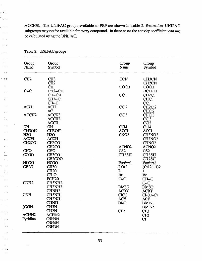
ACCH3). The UNIFAC groups available to PEP are shown in Table 2. Remember UNIFAC subgroups may not be available for every compound In these cases the activity coefficient can not be calculated using the UNIFAC.

Table 2. UNIFAC groups

Group Group Group Group .Name Symbol Name Symbol

CH2 CH3 CCN CH3CN CH2 CH2CN CH COOH COOH

C=C CH2=CH HCOOH CH=CH CCI CH2CI CH2=C CHCI CH=C CO

ACH ACH CC12 CH2CI2 AC CHCl2

ACCH2 ACCH3 CCl3 CHCl3 ACCH2 CCl3 ACCH CC12

OH OH CCl4 CCl4 CH30H CH30H ACCl ACCl H2O H2O CN02 CH3N02 ACOH ACOH CH2N02 CH2CO CH3CO CHN02

CH2CO ACN02 ACN02 CHO CHO CS2 CS2 CCOO CH3CO CH3SH CH3SH

CH2COO CH2SH HCOO HCOO Furfural Furfural CH20 CIDO OOH (CH20H)2

CH20 I I CH-O Br Br FCH20 O==C CH ... C

CNH2 CH3NH2 C ... C CH2NH2 DMSO DMSO CHNH2 ACRY ACRY

CNH CH3NH CICC CI-(C=C) CH2NH ACF ACF CHNH DMF DMF-l

(C)3N CH3N DMF-2 CH2N CF2 CF3

ACHN2 ACHN2 CF2 Pyridine C5H5N CF

C5H4N C5H3N

33

Calculate Activity Coefficients

Mter the functional groups are chosen, the activity coefficients can be calculated using the procedure described by Grain (1990) by clicking on the "Calc. Activity Coefficients" button. Once the activity coefficients have been calculated they can be displayed, along with values from several intermediate steps, by clicking on the "Display Act. Coeff." button. The equations used to calculate the activity coefficients can also be displayed by clicking the "balloon" on the "UNIFAC Calculations" crd.

Editing Parameters

The UNIFAC group values can be edited by clicking on the "Edit Parameters" button. This will take you to an Index card containing a button for each group. To edit the value for that group, click on the corresponding group button. To edit the Q and R values, click on the left arrow at the bottom of the index card

Estimating Properties

To estimate Sand/or Kow click on the "Estimate Properties" button. Clicking the "eye" next to

the property will display the equations used to estimate S or !<Ow. The results will be reported on

the results card.

Limitations of UNIF AC Approach to Estimating Sand Kow

The use ofUNIFAC is limited to chemicals that have subgroups contained in a UNJFAC data

base. If a chemical has subgroups for which no UNIFAC values are available, the activity

coefficients cannot be calculated and, therefore, the properties cannot be estimated. In addition, it has been observed that the errors associated with estimating S and Kow via the UNIFAC approach

tend to increase as the compound becomes less solubility (larger Kow). Correction factors have

been presented. in the literature to correct for this tendency.

34

" "- -

r "

Property/Property Module

Overview

Quantitative Property-Property Relationships (QPPRs), based on the relationship between two properties as determined by regression analysis, are used to predict the property of interest from another more easily obtained property without a specific concern for molecular structure. Frequently, the regression expressions are expressed in terms of the log of the two properties.

The operation of the Property-Property correlation module, illustrated in Figure 20, is considerably different than the other modules because the choice of the regression models used. for the property estimation detennines the required inputs.

PEP Processor 0;

• File Edit Go Print Uiew (1) ~

Prooertv/Prooertv Chemicol Nome:.1.12"J§,6·-tetr:.Q.gjlgrob{".b~JJ.!ll

SMILES String: - -3. I nput Properties

1. Choose 2. Uiew Property @ USER choose regression PEP REF I Loole in Prop. DB I

o PEP choose regression Stots ·-·1 IogS_ ! !Y:,,) i·~-r '.L

1815 I Universal from Kow I @~ log Kow _~-,2.~6_

~t·~ r:--.. -. : ~ tf"·'c: ~ •

DKow H I !.~~·11· .. c11r(ol':: S ~ I r:. I ~~ -t }o{J f. ___ l~{ .. ~· I

~tf(oc ___

181 Koc Universal from Kow ~ @~ 1If900: _

M.fl. '1:: I8J BCF I Universal from Kow ~ @~ ---MY. -----

OH ~ " '" -- i ~~ ..&. • :- ... ",-:<i L_ :

4. Estimat~ ~ Properties

Note: All yulues are at 25°C '::',.::.:'.: , ... "::',. : ... ~~: .. :',:::: .. :: " '::':: ':" . ,:",:' ~ ': .. :.::.~.~. :;.::~.:".~~~~" .. ~ :',: ~~: :: ',:' ...... ': ........ : ~ .; .... '.::.~'" ... ~~ ~.:~. '.:~: ... : .: .. ~:~ ....... ~:"": :"::;"::: " .. ~ "";:: .. "" " . " .: .: .:"::" ." "":"":.".

Figure 20. Example card from PEP property-property module.

35

Selecting the Properties to be Estimated

Since the input for the PropertylProperty module depends on the properties to be estimated and the regression models used, the user must first select the properties to be estimated and the regression equations to be used before any input values are requested. The program keeps track of the properties required and provides the appropriate input fields. If available, the required properties can be imported directly from the associated chemical property database. Currently property-property r~lationships for the estimation of S, Kow, Koc, and BCF are available and will darken as the properties are selected.

Choosing the Property-Property Regression Model

The most appropriate model to use in estimating the property of interest depends on the class of the chemical and what property-property relationships are available. The property-property relationships that are available in PEP are divided into two general categories; regressions developed using data from the PEP Chemical Physical Data Base and regressions obtained from the literature. The two categories are separated by a grey line in the popup menu. To choose the property-property model, use the popup menu directly under the current regression by holding the mouse button down while over the title of the current regression. The "eye" icon to the right of the

regression title will display the regression equation and statistics associated with the current relationship. The "book" icon will show the reference for the current regression if the regression is from the literature.

Viewing the Calculated Values

Once the properties and the relationships are chosen, the properties required for input need to be entered. The properties that are required are shown on the right side of the card with a line next

to the symbol. The values can be retrieved from the PEP Chemical Property Database by making sure the property name is correct and clicking on the "Look in Prop. DB" button. The current units of the inputs will be shown if appropriate, and will be changed as needed by PEP for the different regression equations.

When the "Estimate Properties button is clicked the properties that were input will be used along with the chosen regression eq~ations to estimate the selected properties. If the values for the input properties have not been entered on the Property-Property card the user will be prompted to supply the required values. The property estimates along with the calculated 95% prediction interval, if the statistical information is available, will be placed on the Results card

36

Limitations of the Property/Property Module

One major limitation to the use of property/property relationships is the lack of suitable property values required for input into the regression models. For many new chemicals, no physica1/chemical property information is available. In addition, the quality of the property­property regression model depends on the extent of the database used to develop the relationship. For example, some property-property models are broader thail others in the type and number of compounds used in its development

37

PEP BATCH

Overview

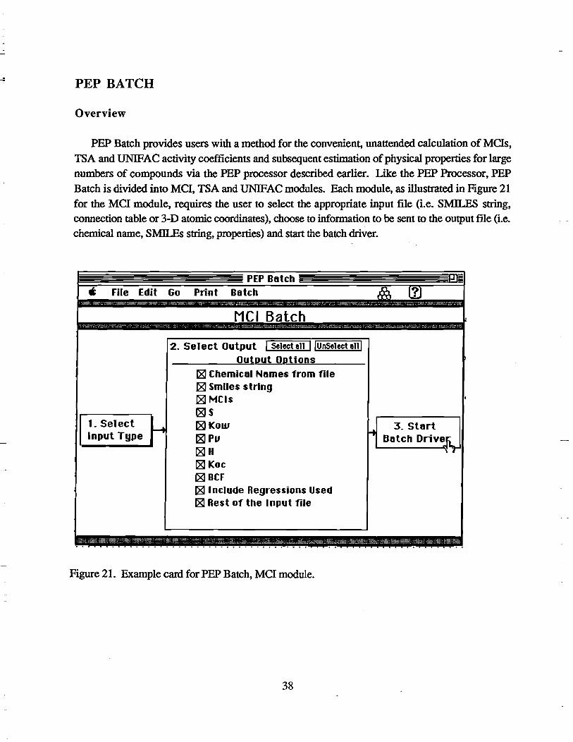
PEP Batch provides users with a method for the convenient, unattended calculation of MCls, TSA and UNIFAC activity coefficients and subsequent estimation of physical properties for large numbers of compounds via the PEP processor described earlier. Like the PEP Processor, PEP Batch is divided into Mel, TSA and UNlFAC modules. Each module, as illustrated in Figure 21 for the MCI module, requires the user to select the appropriate input file (Le. SMILES string, connection table or 3-D atomic coordinates), choose to information to be sent to the output file (i.e. chemical name, SMILEs string, properties) and start the batch driver.

PEP Batch

" File Edit Go Print Batch

L Select Input Type Y

Mel Balch

2. Select Output I Selectell I IUnSelectell I ________ ~O~u~tp_utOp_~t~io~n~s~ ____ _

t8I Chemical Names from file t8I Smiles string t8I MCls t81S t8I Kow t8I PI1 t81H 181 Koc t8I BCF t81lnclude Regressions Used 181 Rest of the Input file

Figure 21. Example card for PEP Batch, MCI module.

38

3. Start ... Botch DriV~

L~

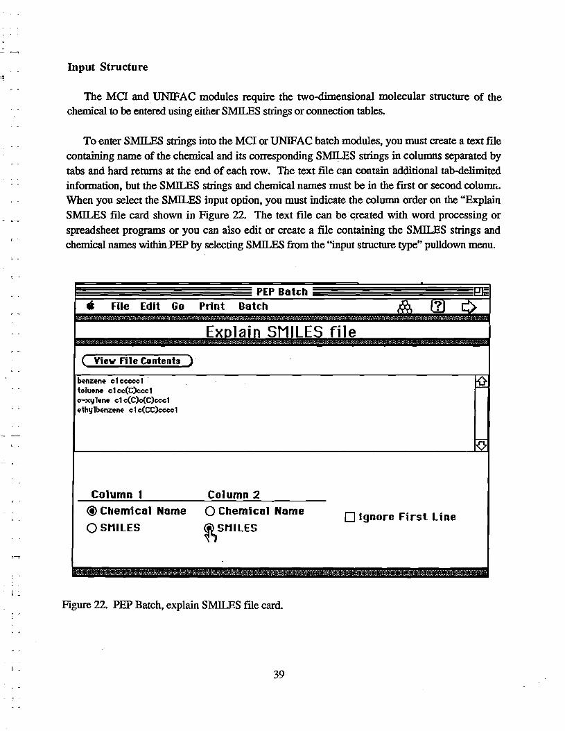
Input Structure

The MCl and UNIFAC modules require the two-dimensional molecular structure of the chemical to be entered using either SMILES strings or connection tables.

To enter SMILES strings into the MCl or UNIFAC batch modules. you must create a text fIle containing name of the chemical and its corresponding SMILES strings in columns separated by tabs and hard returns at the end of each row. The text fue can contain additional tab-delimited infOlmation. but the SMllES strings and chemical names must be in the lust or second coluDlIi.. When you select the SMILES input option, you must indicate the column order on the "Explain SMILES fIle card shown in Figure 22. The text fIle can be created with word processing or spreadsheet programs or you can also edit or create a fIle containing the SMILES strings and chemical names within.PEP by selecting SMILES from the "input structure type" pulldown menu.

PEP Botch ~

• File Edit Go Print Botch &2, ~ 0 Exolain SMILES file

( View File Contents ) benzene c 1 cccce 1 . ~ tol~M cl cc(C)ccel o-xylene cl c(C)c(C)cccl .thy lbenzene c 1 c(CC)ccce 1

~

Column 1 Column 2

@ Cherni col Nome o Chemical Nome o Ignore First line OSMllES ~SMllES

:; .. :'.: ': :'. : .... :',: ': .. :':: . " .:" ;:' ::':n::, . . ' .. : " ":. ", ':: ·::"::.·:m~ .. :~:C; .. :: .. ;::; .. :~ .: ....... :::.::~:;~:.:..; :-""'::"~:';···.~·:·::;:::;;::n::n::;: n;::':':;~::; : ......... :', :·:.:·:· .. ::; .. ·: ..... :L;::;;:: .. ;::. ::; : .. :: .......

Figure 22. PEP Batch, explain SMILES fIle card.

39

To input connection table files into the MCl or UNlFAC batch modules, you must fIrst place

them in a single folder. Select the "Connection tables" option from the "Select Input Type" popup

button and choose the folder that contains the connection table files using the standard "open fIle"

dialog box that appears. Highlighting anyone of the fIles in the folder selects all of the fIles in that

folder and allows you to view or delete specifIc fIles. The fIles can be any valid type for the MCl

module as they will be converted if possible (see MCl module helps). After selecting the input

fIles, click on the advance arrow located at the upper right of the card to advance to the next step.

The TSA batch module operates in the same manner as the MCl and UNIFAC modules except

that the calculation of TSA requires the three-dimensional cartesian coordinates for each atom in the

chemical of interest The TSA batch module accepts Cartesian Coordinates or Alchemy fIles.

Alchemy fIles contain both the two-dimensional chemical structure and the coordinates. This

allows PEP to calculate the chemical's TSA and determine the most appropriate TSA-property

relationship based on chemical class. From within the standard dialog box, you can click on any

fIle in a folder to select all of the fIles in that folder. The fIles will then be displayed. You can

also view or delete fIles.

Output Options

Once the input fIles have been selected, the "output option" step becomes active. This allows

the user to select the properties to be calculated and any additional infonnation that is available (Le.

chemical name, SMILES string, MCls, TSA, or UNIFAC activity coefficients) to be exported by

to a tab-delimited text fIle.

Start Batch Driver

After the output information is selected, the "Start Batch Driver" button becomes active.

Clicking this button brings up the standard Macintosh "save fIle" dialog box that allows the user to

specify the name of the data fIle to be exported by PEP batch and the location that the fIle will be

saved.

40

CHEMICAL PROPERTY DATABASE

Overview

Experimentally determined physical property data for about 800 compounds, having at least one value of aqueous solubility (S), octanoVwater partition coefficient (Kow), vapor pressure (Pv), organic carbon normalized soil sorption coefficient (Koc), bioconcentration factor (BCF), or Henry's law constant (H), was complied from a variety of literature sources and computerized databases. Using this information, a chemical property database was constructed using HyperCard™ and subsequently used for developing MCI-property, TSA-property and property­property relationships. In addition to the properties listed' above, the database includes the following information: compound name and synonyms, a diagram of the 2-D chemical structure, SMILES notation, uses, CAS number, chemical formula, molecular weight (MW),. boiling point (BP), melting point (MP), and appropriate references for each value. A built-in unit conversion utility enables users to quickly view property values in a variety of commonly used units. The database is directly connected to the PEP Processor stack.

The Chemical Property Database also provides the means for the user to search for chemical compounds by full or partial name or synonym, to sort the compounds by name, boiling point, melting point, or molecular weight, and the ability to transfer to any of the property estimation modules. In addition, the user can easily edit exiting values, add new values or export information to a text file or another database.

In addition to the physical properties, information describing the environmental persistence and toxicity of specific chemicals can also be entered into the database. Placeholders for biodegradation rates, hydrolysis rates, photolysis rates and LC50s, along with the appropriate references and comments have been incorporated into the database. This feature was added to the database after requests from test users, however currently no degradation or toxicity data has been entered into the database. The chemical property database is illustrated in Figures 23 and 24.

41

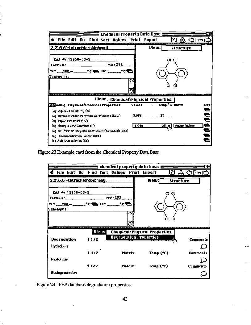
Chemicol Property Ooto Bose • File Edit Go Find Sort 1I0lues Print EHport

.2.2." .6 .6" -tetnlchl orobiDhenyl lliew: ,-I __ s_t_ru_c_t_u ... re ____ 1

CAS #: 15968-05-5 ClCl rormula: _______ _ HV: 292

HP:_~-___ Oc~ BP: ___ oc~

Cl Cl

lIiew: j Chemicol\Physicol Properties' ~tf1og "',sic.1llla._ic.1l1 Pr.p~rties V.1l~s T~mpoc Units

'109 A~ous Solubility (S) '109 OcbnolNatw P~ion Co.ff"lCWnU (Kow) .,,5""'.9"'36""--___ -"'2,.,.5 __

'109 Vapor Prusun (Pv)

R~f

~ ~ ~

...,...----,,.....,.-;----,.~ '109 ~'1I's Law CoI\St~t (H) .. 1-_1.iOO64oiii8 ______ 2;;;:5~fiIIl dimension~ss

'109 SoilN",ter Sorption Co.ff"lCWnt (oc-bueti) (Koc) ~ '109 Oioconcfl\tration Factor (Ocr)

'109 Acid Dissociation (K",)

Figme 23 Example card from the Chemical Property Data Base

CAS #: 15968-05-5 Fermul.1l: _______ _

Degradation

Hydrolysis

Rlotolysis

Biodegr ad ation

t 112

t 1/2

MV: 292

Metrix

Metrix

Figure 24. PEP database degradation properties.

42

ClCl

Temp (-C)

~ ~ ~

Cemments

D Comments

D Comments

D

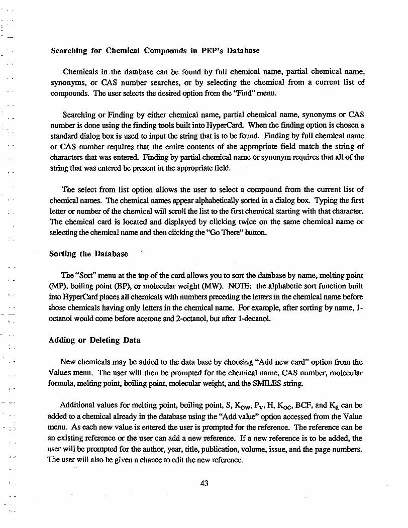
L ~

Searching for Chemical Compounds in PEP's Database

Chemicals in the database can be found by full chemical name, partial chemical name, synonyms, or CAS number searches, or by selecting the chemical from a current list of compounds. The user selects the desired option from the "Find" menu.

Searching or Finding by either chemical name, partial chemical name. synonyms or CAS number is done using the finding tools built into HyperCard. When the finding option is chosen a standard dialog box is used to input the string that is to be found Finding by full chemical name or CAS number requires that the entire contents of the appropriate field match the string of characters that was entered Finding by partial chemical name or synonym requires that all of the string that was entered be present in the appropriate field.

The select from list option allows the user to select a compound from the current list of chemical names. The chemical names appear alphabetically sorted in a dialog box. Typing the first letter or number of the chemical will scroll the list to the flfSt chemical starting with that character. The chemical card is located and displayed by clicking twice on the same chemical name or selecting the chemical name and then clicking the "Go There" button.

Sorting the Database

The "Sort" menu at the top of the card allows you to sort the database by name, melting point (MP). boiling point (BP). or molecular weight (MW). NOTE: the alphabetic sort function built into HyperCard places all chemicals with numbers preceding the letters in the chemical name before

those chemicals having only letters in the chemical name. For example. after sorting by name. 1-octanol would come before acetone and 2-octanol. but after 1-decanol.

Adding or Deleting Data

New chemicals may be added to the data base by choosing "Add new card" option from the Values menu. The user will then be prompted for the chemical name. CAS number. molecular formula, melting point, boiling point, molecular weight, and the SMILES string.

Additional values for melting pOint. boiling point, S. Kow, pv• II, Koc. BCF, and Ka can be

added to a chemical already in the database using the "Add value" option accessed from the Value menu. As each new value is entered the user is prompted for the reference. The reference can be

an existing reference or the user can add a new reference. If a new reference is to be added. the

user will be prompted for the author. year, title. pUblication. volume, issue, and the page numbers. The user will also be given a chance to edit the new reference.

43

An entire card or specific values contained on a card can be deleted by choosing the appropriate item from the Value menu. A reference can also be deleted if it was entered incorrectly. The data will not be deleted until the user verifies the request through a standard dialog box.

Printing Information From the Database

The user can print the current card, or a series of cards using the print features built into HyperCard. To print a series of cards, flISt the user must select that option from the "Print" menu. Then while each card that is to be printed is the currently displayed card, the select "Print this card" option from the print menu must be chosen. When the desired cards have been printed, the user then selects "Stop printing" from the "Print" menu. The user can also print a list of all the references contained in the PEP data base.

Exporting Information From the Database

Infonnation in the database can either be exported as text in a line or as a spreadsheet format

using the ''Export'' menu. If the line fozmat option is used, the data will appear with each data field on a line and each chemical separated by a solid line. This option is most appropriate if a word processor will be used to print or manipulate the exported data. If the spreadsheet format is used the data will be put in columns delimited by a tab.

Moving to Other PEP Modules

The "Go" menu at the top of the card allows you to move to any PEP module. To use the Go option, move the pointer to Go menu at the top of the card. Hold the pointer down on the button

until the selections appear. Then move the pointer until the selection of choice is highlighted and release the mouse button.

Changing the Units of Measurement

The popup menu under each property's units allows you to change the units for solubility,

Henry's law, and vapor pressure. All values of the property will be changed to reflect the new units.

44

- [:

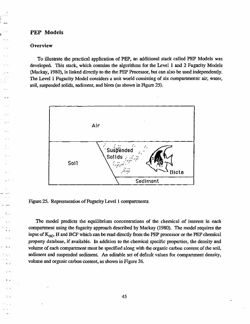
PEP Models

Overview

To illustrate the practical application of PEP, an additional stack called PEP Models was developed. This stack, which contains the algorithms for the Levelland 2 Fugacity Models (Mackay, 1980), is linked directly to the the PEP Processor, but can also be used independently. The Levell Fugacity Model considers a unit world consisting of six compartments: air, water, soil, suspended solids, sediment, and biota (as shown in Figure 25).

Air

Soil

. . .. .. .. . Sus·p'ended So11 ds .... : .. :.:

.'" .. .o .. " .,".:." " ...

...... : ........ : .. . '"" .. .. ": .. '":'". . .

..

Sediment

Figure 25. Representation of Fugacity Levell compartments.

The model predicts the equilibrium concentrations of the chemical of interest in each compartment using the fugacity approach described by Mackay (1980). The model requires the input of Koc, H and BCF which can be read directly from the PEP processor or the PEP chemical

property database, if available. In addition to the chemical specific properties, the density and volume of each compartment must be specified along with the organic carbon content of the soil, sediment and suspended sediment An editable set of default values for compartment density, volume and organic carbon content, as shown in Figure 26.

45

PEP Models BJ~

• file Edit Go Print Comportments ~~(l)

Fugacity Model

Chemical Name: 2.2-.6.6--tetrachloroblphenyl 1_lnput 2_ Input Enuironmentol Comportment Ualues

Property Uolues

[5J Comportment Density Uolume % Orgonic YUiesin

Icg/m~ m!! Corbon PrGp.D8

~ 3. C8lculot~ ~

log Kot 0 [81 Air J.J..2- lelQ_ Distribution i

13.92 1 f-t [8IllIoter J..900 .7e6 _ OR log H 181

J.~HOO _ge3 _4.. __ \ Input Fugacity (4mensio1iless) [81 Soil 1-1.648 1 181 Susp. Solids _ L~HOO -~-- _4. __ Level 2 Data

log BCf 0 181 Sediment J.5..00 _~.1 e'~L -4 ... _ 14.69 1 181 Biota J..9_00 -~-181 IDdicates

value fre .. DB

....... . ...... ......... ......... .......... ............ "..... . ...... ......... ............ ............. . .......... ...... ..... : .. :.~ .. ~ .. ~ .... ,~~:.::; ... u~~ .. ,.\\,;::.;:;~.u.,~ .. ...... ~ ... : ..... ::: ...................... ;:;:~::: ..................... ~,l ..... ::::ut"o ........... w ......... ~ .. : .................... ~~:;~g: .. M ... w ..... ; ...... :~~L ........... v ......... ~;;:.::.nN .... Y.w ... <~:;:~.::: ... v .. n'" ..... <~::;~ .. t:

Figure 26. PEP Models card, input for Fugacity Level 1

The Level 2 Fugacity Model allows for the chemical of interest to degrade in each compartment, move by advection through the water and air phases, and be emitted into the unit

world. The rate values for each of these processes must be entered by the user. The degradation rates for each compartment can be entered either by t1/2 values in hours or by fIrst order reaction rate constants in l/hours, as shown in Figure 27. The advection rate data can be entered either by residence time or flow rate and the concentration or by directly entering the mass flow rate in moles per hour. The emission rate is entered in the units of moles per hour.

46

- ~-:

L ~

- r:----:J

Edit Go Print Rotes

Level

Chemicol Nome: 2,2· ,6,6·-tetrochlorobiphenyl

181 Air

181 Water

181 Soil

181 SUsp. Solids

181 Sediment 181 Rioto

~--------------------------~ 3. Input Reaction Rote Doto 4. Input Advective Dato (input reaction 1121ife or (input m~s flo .... rete or conc. and reaction rate constant) residence time or flo,"" rete}

Reaction Re6ction tl2life OR rate const holrs hours-t

Residence Flow Ume OR Rate hours m3 /hr

Mess Cone. flow rate

mol/m3 mol/hr

----- --_ •••••• - ... -_ ••••• _.- "::":';:<':::--='::"1

5. Input Emission Rate

Emission rote mol/hr

Figure 27. PEP Models card, input for Fugacity Level 2

Input Property Values

To calculate the environmental distribution of a chemical the user must enter the several physical-chemical properties along with the size and densities of each compartment The physical­chemical properties that are need to be input for the six compartment unit world are Koc, H, and BCF. However, in step 2 the user may choose to eliminate one or more compartments to simplify the model or to more closely examine the distribution ofa chemical in a sub-environment such as the hypolimnion of a lake (i.e., water, air, biota). This would eliminate the need for a value for Koc. PEP determines which physical-chemical property values are needed depending on the unit

world which the user has defmed. The chemical-physical properties that are not needed will be dimmed.

When available, experimental values are preferred over estimated values in environmental fate modeling. Experimental values for the physical-chemical properties can be searched for in the Chemical Property Data Base by using the ''Look for Values in Prop.DB" option. When clicked, a

47

full chemical name search is initiated, and if the chemical is found, the values of the three properties required by the Fugacity level 1 model will be displayed in a dialog box. The values can be copied to the Fugacity card using the buttons on the dialog box as illustrated in Figure 28. The check boxes next to the property names of the Fugacity card indicate if the property came from the data base.

Ualues from the PEP Property Catabase

Select the properties to copy to the Model

Log Koc: 1.780 ~ ( Cancel ) Log H: -0.648 Log BCF : Not Found ( Copy nil )

10 € Copy Selected ~

Figure 28. Example dialog box resulting from the "Look for Values in PropDB" option

Input Environmental Values

The values used for the unit world can be changed in step 2. The available compartments are air, water, soil, suspended solids, sediment, and biota. Water must always be part of the unit world because of the partition coefficients are defined as the ratio of the chemical in the non­aqueous phase to the aqueous phase. The rest of the compartments can be eliminated by clicking the check box next the compartment name. The densities, volumes, and the percent organic carbon (if appropriate) of each compartment can be changed.

Different user dermed environments or unit worlds can also be saved using the "Save Current Values" button and later recalled using the "Values:" popup menu. The "Delete Saved Values" button can be used to remove a saved set of values from the list that will popup when the "Values" button is used. The "Set Default V a1ues" button can be used to set the unit world that is used when the PEP Models stack is opened.

Calculate Distribution

After the user inputs all the required infonnation and hits the "calculate distribution" button, the model ca).culations are perfonned in HyperTalk and the results are presented in both in tabular and

48

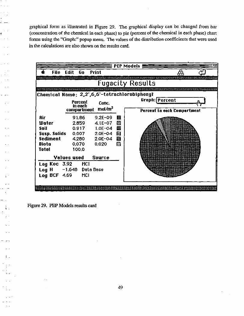
- t--:;

r '

graphical form as illustrated in Figure 29. The graphical display can be changed from bar (concentration of the chemical in each phase) to pie (percent of the chemical in each phase) chart fonns using the "Graph:" popup menu. The values of the distribution coefficients that were used

in the calculations are also shown on the results card.

PEP Models • File Edit Go Print

Fugacity Resu1ts

Chemical Nome: 2,2·,6,6·-tetrochlorobiphenyl

Air Woter Soil Susp.Solids Sediment Bioto Totol

~ercent Conc. Gnph:I~P-e-r-c-e-nt-:-----"'--" 10 eoch!'.l ~.,..

compartment mollm Percent in each Compartment

91.86 2.659 0.917 0.007 4.260 0.070 100.0

9.2E-09 iii 4.1E-07 ~ 1.0E -04 II1II 2.0E-04 1m) 2.0E-04 II 0.020 ~

Vo) ues used Source Log Koc 3.92 MCI Log H -1.646 06t6 56se Log BCF 4.69 MCI

Figure 29. PEP Models results. card

49

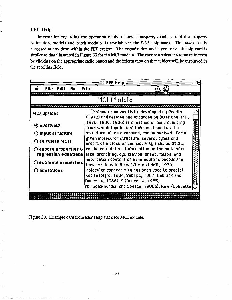
PEP Help

Infonnation regarding the operation of the chemical property database and the property estimation, models and batch modules is available in the PEP Help stack. This stack easily accessed at any time within the PEP system. The organization and layout of each help card is similar to that illustrated in Figure 30 for the MCl module. The user can select the topic of interest by clicking on the appropriate radio button and the infonnation on that subject will be displayed in the scrolling field.

PEP Help • File Edit 60 Print

MCIOptions

@oueruiew

o input structure

o calculate MCls

MCI Modu1e

Molecular connectivity developed by Randic (1972) Bnd refined and expanded by (Kier and Hall, 1976, 1980, 1986) is a method of bond counting from which topological indexes, based on the structure of the compound, CBn be derived. For B given moleculBr structure, seyerBl types Bnd orders of molecular connectivity indexes (Mels)

o choose properties 6' CBn be cBlculBted. InformBtion on the molecular regression equations size, branching, cyclizBtion, unsaturation, end

o estimate properties

o limitations

heteroetom content of a molecule is encoded in these yanous indices (Kier Bnd Hall, 1976). Molecular connectivity has been used to predict Koc (Sebljic, 1984, Sabljic, 1987, Bahnick and Doucette, 1988), 5 (Doucette, 1985, NirmalakhBnd8n and Speece, 19888), Kow (Doucette

Figure 30. Example card from PEP Help stack for MCl module.

50

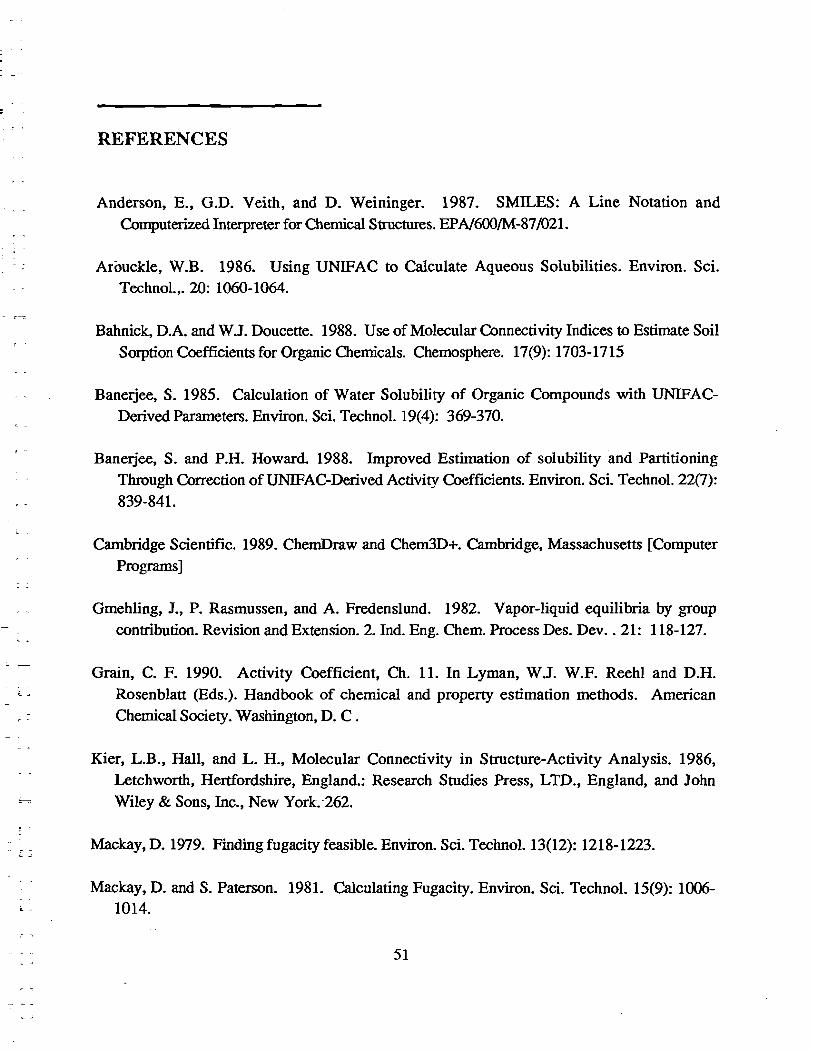
l j

REFERENCES

Anderson, E., G.D. Veith, and D. Weininger. 1987. SMaES: A Line Notation and Computerized Interpreter for Chemical Structures. EP N600/M-87/021.

Arouckle, W.B. 1986. Using UNIFAC to Calculate Aqueous Solubilities. Environ. Sci. Technol.,. 20: 1060-1064.

Bahnick, D.A. and W.J. Doucette. 1988. Use of Molecular Connectivity Indices to Estimate Soil Sorption Coefficients for Organic Chemicals. Chemosphere. 17(9): 1703-1715

BaneIjee, S. 1985. Calculation of Water Solubility of Organic Compounds with UNIFAC­Derived Parameters. Environ. Sci. Technol. 19(4): 369-370.

BaneIjee, S. and P.H. Howard. 1988. Improved Estimation of solubility and Partitioning Through Correction of UNIFAC-Derived Activity Coefficients. Environ. Sci. TechnoL 22(7): 839-841.

Cambridge Scientific. 1989. ChemDraw and Chem3D+. Cambridge, Massachusetts [Computer Programs]

Gmehling, J., P. Rasmussen, and A. Fredenslund. 1982. Vapor-liquid equilibria by group contribution. Revision and Extension. 2. Ind. Eng. Chern. Process Des. Dev .. 21: 118-127.

Grain, C. P. 1990. Activity Coefficient, Ch. 11. In Lyman, W.J. W.P. Reehl and D.H. Rosenblatt (Eds.). Handbook of chemical and property estimation methods. American Chemical Society. Washington, D. C.

Kier, L.B., Hall, and L. H., Molecular Connectivity in Structure-Activity Analysis. 1986, Letchworth, Hertfordshire, England.: Research Studies Press, LTD., England, and John Wiley & Sons, Inc., New York. -262.

Mackay, D. 1979. Finding fugacity feasible. Environ. Sci. Techno!. 13(12): 1218-1223.

Mackay, D. and S. Paterson. 1981. Calculating Fugacity. Environ. Sci. Technol. 15(9): 1006-1014.

51

Pauling, L. 1960. The nature of the chemical bond. Cornell University Press, Ithaca, New York 262 p.

Pearlman, R.S. 1980. Molecular surface areas and volumes and their use in structure/~ctivity relationships, p. 331-346. In S.H. Yalkowsky, A.A. Sikula and S.C. Valvani (Eds.). Physical chemical properties of drugs. Marcel Dekker, Inc., New Yorlc.

Tripos Pssociates Inc. 1989. Alchemy and CONCORD. St. Louis, Missouri [Computer Programs]

Weininger, David. 1988. SMILES, a chemical language and information system. 1. Introduction

to methodology and encoding rules. 1. Chern. Inf. Comput. Sci. 28:31-36.

52