ISSN 1745-8587 B

irkbe

ck W

orki

ng P

aper

s in

Eco

nom

ics

& F

inan

ce

School of Economics, Mathematics and Statistics

BWPEF 0606

Pricing Multiple Interruptible-Swing Contracts

Marcelo G Figueroa

May 2006

Birkbeck, University of London Malet Street London WC1E 7HX

Pricing MultipleInterruptible-Swing Contracts

Marcelo G. Figueroa ∗

Birkbeck College, University of London

First version: December, 2005This version: May 4, 2006

Abstract

In this article we price a multiple-interruptible contract for the electricitymarket in England and Wales under a mean-reverting jump-diffusion modelwith seasonality. We do so by combining forward contracts with a swing optionwhich can be exercised a pre-specified number of times. We price this swingoption by means of an extension of the Least-Squares Monte Carlo methodologyfor American options. We additionally compute the lower and upper boundsfor this contract. For the computation of the lower bound we provide a semi-analytical formula which reduces greatly the required computational time.

Keywords: Energy derivatives, electricity market, Least-Squares Monte Carlo,swing options.

1 Introduction

One of the objectives of NETA (New Electricity Trade Arrangement), introducedon March 27, 2001 was to remove price controls and openly encourage competitionby providing greater scope for demand-side participation in the electricity market,thereby ensuring a more efficient means of meeting consumption requirements on thesystem. By creating a system where the value of short-term portfolio flexibility (torespond to short-term price spikes or to hedge exposure to imbalance charges) wasmore transparent to market participants, it was anticipated that there would be anincrease in the elasticity of price-responsiveness in the market.

∗Email: mfigueroa@econ.bbk.ac.uk

1

Interruptible contracts, where a supplier has the right to cease supply to a con-sumer under pre-defined conditions, have been a major tool for introducing demand-side flexibility in other markets, such as the gas market. Until now, such contractshave been utilized by the NGC (National Grid Company) as part of its balancingservices obligations, but have not developed significantly as an option in standardcommercial contracts. As technology improvements make the use of such arrange-ments less costly, the key questions are whether such contracts have a real value inelectricity markets and how that would translate into contract terms and prices.

In general, an interruptible contract can be considered as a standard supply con-tract with the following additional conditions on physical delivery: a specified number,or volume, of interruptions that can be called over the life of the contract; a minimumnotification period prior to each interruption; and a minimum and maximum periodfor each interruption called.

The value of the flexibility implied in these conditions would be reflected in thecontract price through, for example, discounted unit electricity prices and/or lump-sum payments per interruption. The exact format of the pricing arrangements woulddepend on both the value to the supplier, the cost to the consumer, and the attitude ofeach party to the underlying risk in the contract. Moreover, a contract which encom-passes all the various flexibilities outlined above has a relatively complex valuationprocess, but fundamentally stems from valuing a swing option.

Electricity contracts which address interruption of supply have been presented inthe past. Gedra [7] introduces the concept of a callable-forward, which is an optionthat results from taking opposite positions on a forward contract and a call option. Asupplier will be able to replicate a simple interruptible contract by shorting a forwardwith maturity T –which commits the supplier to deliver one unit of energy (denotedby St) at time T for the pre-specified price F T

t , and longing a call option with equalmaturity written on the same unit of energy. Hence, the supplier’s portfolio at time tis given by Πt = −F T

t + C(St; K,T ), where K is the strike price of the option, whichis taken as the shortage cost a potential user faces when curtailed.1

Since the supplier buys the call, he has the right to exercise the call option atdelivery. At expiry, his portfolio is worth ΠT = −ST + max (ST −K, 0), since F T

T =ST . If at expiry the price of electricity is higher than the strike price, the supplier

1In order to avoid confusions at a later stage, it is important at this point to clarify the notation.It is typical in the financial mathematics literature to refer to the forward price of a contract as ft,whose payoff at delivery time T is ST − χ, where χ is the price of the forward contract at time Twhich guarantees that at time t0, when the forward is contracted, the forward contract f0 has zerovalue (since the price of the forward is settled at expiry). The forward FT

t to which we refer andwhich is calculated as the expected value of the spot price under an equivalent martingale measureis in this context χt and is such that at t = T we recover the spot price.

2

will exercise the call option; consequently, the unit of energy ST is canceled and thesupplier pays the consumer the strike price K in compensation. On the other hand,if the observed price of electricity is lower than the strike price, the option will notbe exercised and the supplier faces the obligation of delivering a unit of energy.

By offering a discount on the forward sold (the value of the call option), thesupplier benefits by earning the possibility of calling off supply in case the price ofelectricity spikes at expiry. On the other hand, the consumer entering this contractbenefits by receiving a discount on the value of the forward he is contracting; sincehis portfolio is worth at any given time t, Πt = F T

t − C(St; T ). In addition to thisdiscount, if, at expiry, the supplier decides to exercise the option, he will curtailsupply but compensate the consumer with the cost of the shortage, K.

A consumer entering into such a contract must trade off the probability of inter-ruption against the cost of the contract. This means that the consumer must tradeoff this probability against the shortage cost associated with his particular business.The probability of interruption decreases as the strike price K increases. As a conse-quence, the call option becomes less valuable, and the discount on the forward priceis lower. On the other hand, those consumers with lower shortage costs will be morelikely to be interrupted and will receive higher discounts.

Although callable forwards succeed in replicating an interruption strategy, a cleardrawback of this type of contract is that there will be consumers whose short-noticeinterruption costs are too high, and these short-notice interruption costs may notprovide a viable strike price for the contracts. Kamat and Oren [13] argue that apossible solution to this would be to introduce an earlier notification date where noticeof interruption is given prior to curtailment. This certainly represents an improvementwith respect to the simple callable-forward discussed earlier, and principally, underwell known frameworks the valuation of such an option is still tractable. Kamatand Oren [13] price this option replicating the payoff with a compound call optionon the forward and present results for a geometric Brownian motion GBM, a meanreverting model and an affine-jump-diffusion. However appealing this model is, theassumption of assuming only one early exercise point is still unrealistic and does notseem to capture the real needs and flexibilities that both consumers and generatorsseek for in these contracts.

We extend these works by substituting the call option on the underlying for anup-swing option (a call-swing option) which allows the holder to exercise N timesfrom a total of M sampling dates. Hence the portfolio the supplier now owns is givenby Πt = −F T

t + Csw(St; K, T ), where we can think of the forward F Tt in any of two

ways. It can either be the market quote for daily delivery across the period [t, T ]of one unit of electricity Su for t ≤ u ≤ T or a sum of theoretical values of the

3

forward for which F Tt =

∑ti=Tti=t+1 F ti

t . In any case, when exercising N times the swingoption we will be canceling delivery of electricity (and compensating the user withthe strike price K) in the corresponding N dates. The user benefits from holding theopposite portfolio, hence the up-swing option represents the discount on the forwardcontracted for the period.

We also extend this valuation to include putable forwards, which result from aportfolio encompassing a forward and a down-swing option. For instance, let usconsider a consumer who owns the following portfolio: Π∗

t = F Tt + P sw(St; K,T ),

he will be prepared to pay a premium above the forward price in order to have thechoice of exercising the down-swing option and therefore selling back to the suppliera unit of electricity at a fixed price K. He will do this only if the price of the spotat the N dates he chooses to exercise is sufficiently low. Since F T

T = ST he will thencancel the delivery from the supplier on those dates and buy on the spot market cheapelectricity, realizing a profit K − Sti , where ti is any of the chosen exercise dates. Onthe other hand, if exercise doesn’t take place, he is still guaranteed delivery of a unitof energy.

Regarding the structure of the swing option, we consider an option of the followingcharacteristics: the swing option can be exercised on a single day a number of N -timespre-specified in the contract; in each exercise opportunity the holder will exercisethe full volume for a strike price K, which should reflect the customer’s cost ofinterruption.2

The pricing of this contract entices two complexities. First, we need to choose asuitable model for the type of market in which we are pricing. As the literature inelectricity derivatives now largely suggests, among spot-based models there is strongconsensus in that models should include the following characteristics in the spot-pricedynamics: mean reversion, seasonality and spikes. These properties have been studiedand analyzed by different authors. For instance Escribano et. al. [2] calibrate thesemodels to different electricity markets to find evidence of mean reversion and spikes.Geman and Roncoroni [8] analyze in detail the fine structure of electricity prices andBenth and Koekebakker [3], apart from providing a thorough discussion of how theNordic power market (Nord Pool) is organized, apply both spot-based models withmean reversion, seasonality and jumps and forward-based models in their discussion.In this application we price under the mean-reverting jump-diffusion (MRJD) modelwith seasonality presented by Cartea and Figueroa [1], slightly modified from itsoriginal version to capture positive and negative exponential jumps, as in Brechner,Cartea and Figueroa [4]. Apart from arguing a case for both positive and negative

2In this case, the interruption is an ‘all or nothing’ choice -i.e. either all the electricity is deliveredon the day or none at all; although this can easily be modified.

4

jumps in electricity markets, the inclusion of exponential jumps simplifies the resultsand enables us to obtain a more tractable option formula.

The second complexity not only involves the American feature of this contract butthe additional difficulty introduced by the swing option of allowing for N exercise op-portunities within the choice of a set of M different sampling dates. American options,or Bermudan options more precisely since we price in a discrete set of sampling dates,are priced using numerical schemes since analytical solutions are not available. Thesenumerical schemes fall broadly in one of three possibilities: discretizations of thepartial differential equation of the problem, which leads to finite-difference schemes;binomial/trinomial-tree-based models; and Monte Carlo techniques. The presence ofjumps give rise to non-local operators, or partial-integral differential equations, whichmake the use of finite difference techniques more complex to apply. Methods based onthe tree dynamic programming approach are relatively simpler to implement. For in-stance, Jaillet, Ron and Tompaidis [12] price swing options based on a multiple-layertree extension of the classical binomial tree.

Finite-difference schemes and trees are well suited for low dimensional problemsand standard dynamics which do not incorporate jumps -i.e. up to three statevariables and log-normal or mean-reverting Gaussian processes. In recent yearsstochastic-mesh methods and regression-based methods based on Monte Carlo tech-niques (see for example Glasserman [9]) have been developed for the pricing of Amer-ican options as an alternative. These methods on the other hand, are suitable forproblems of higher-dimensions and can handle stochastic parameters as well as jumps.In particular in this paper we will price a swing option by modifying the Least-SquaresMonte Carlo (LSM) algorithm proposed by Longstaff and Schwartz [17] to allow formultiple exercise. Finally, we should also mention that within the Monte Carlo meth-ods an alternative to the above LSM methodology has been presented by Ibanez andZapatero [11], where they compute directly the optimal exercise frontier rather thanestimating by regression the continuation value at each exercise point. Moreover,Ibanez [10] applies this algorithm to the specific valuation of swing options. In thispaper we compare our results obtained through an extended LSM algorithm for swingoptions to those obtained by Ibanez [10].

Finally, we present semi-analytical formulæ to price vanilla options under theconsidered MRJD model which enables us to compute the lower bound for the swingoption at least 100 times faster than by pricing the vanilla options with Monte Carlotechniques.

The remaining of this article is organized as follows. In Section 2 we review themodel in Cartea and Figueroa [1] and present the semi-analytical pricing formulæ inorder to price the lower bound for the price of the swing option more efficiently. In

5

Section 3 we discuss the valuation of the swing option with an extension of the LSMalgorithm. In Section 4 we present the results and finally in Section 5 we conclude.

2 The European Pricing formula

In this section we discuss the pricing of a call option under a MRJD model withseasonality using complex fourier transforms (CFT) in order to set a lower bound forthe contract.

Cartea and Figueroa [1] derive a closed-form analytical solution for the forward,however, the pricing of vanilla instruments is not discussed. Here, we extend thatwork to provide a semi-analytical solution for vanilla options under this model. Weprovide option formulæ for both an option written on the underlying itself, i.e. thespot price of electricity; and an option written on a forward for a unit of electricity.

Lemma 2.1 Let Yt be the underlying state variable representing any class of exponen-tial Levy process such that Et

[eYT

]< ∞, YT (Yt) the underlying at time T conditional

on Yt, VT (ξ) the transformed payoff of the option and Ψ(ξ) the characteristic func-tion, defined as Ψ(ξ) := Et

[eiξ ln YT

]. Then the price of a T -maturity European option

written on the underlying Yt with strike price K is given by

V (Yt, t) =e−r(T−t)

2π

∫ ∞+ib

−∞+ib

Ψ(−ξ)VT (ξ)dξ, (1)

where ξ := a + ib, and a, b ∈ R. The integration can be performed along any closed-curve within the contour defined by the intersection of the strip of regularities definedby the transformed payoff and the characteristic function.

Lewis [16] shows that this pricing formula can be applied to any class of expo-nential Levy processes such that Et

[eYT

]< ∞. In particular this encompasses for

instance the Black-Scholes model, Merton’s jump-diffusion model, the jump-diffusionmodel of [14] and all other classes of pure jump models.3

Cartea and Figueroa [1] show that the stochastic-differential equation (SDE) onthe spot price can be integrated to yield

ST = eg(T )+(xt−gt)e−α(T−t)−λR T

t σse−α(T−s)ds+R T

t σse−α(T−s)dZs+R T

t ln Jse−α(T−s)dqs , (2)

where g(T ) is the logarithm of the deterministic seasonality function, α is the mean-reversion rate, σ(t) the volatility, λ the market price of risk, dZt the Brownian incre-ment under the risk-neutral measure; Js the jump at time s which is drawn from alog-normal distribution and dqt a Poisson process with intensity parameter l.

3Formal proofs can be found in [15].

6

They also provide a closed-form solution for the forward at time t maturing attime T ′, which can be written as

F T ′t = eg(T ′)+(xt−gt)e−α(T ′−t)−λ

R T ′t σse−α(T ′−s)ds+ 1

2

R T ′t σ2

se−2α(T ′−s)ds+R T ′

t (Et[eαs ]−1)lds, (3)

where αs := e−α(T ′−s) ln Js.

Cartea and Figueroa [1] assume the logarithm of the jumps are drawn from a nor-mal distribution. Brechner, Cartea and Figueroa [4] have modified this by assumingexponential jumps, as introduced in Kou [14]. This is, it is assumed that Y = ln Jhas an asymmetric double exponential distribution with density

fY(y) = pη1e−η1y1y≥0 + qη2e

η2y1y<0, (4)

where η1 > 1, η2 > 0, and p,q ≥ 0 are such that p + q = 1. Moreover, p and qrepresent the probabilities of upward and downward jumps, respectively.

Apart from arguing a case for both positive and negative jumps in electricitymarkets, the inclusion of exponential jumps simplifies the results and enables us toobtain a more tractable option formula.4

2.1 Pricing on a forward

By assuming positive and negative jumps drawn from the double exponential distri-bution in (4) the forward in (3) becomes

F T ′t = G(T )

(S(t)

G(t)

)ht

e12

R T ′t σ2

sh2sds−λ

R T ′t σshsds− kl

α(1−ht)

(η2 + ht

η2 + 1

) qlα

(ht − η1

1− η1

) plα

,

(5)where G(t) is the deterministic seasonality function, σ(t) is the time-dependantvolatility, λ is the market price of risk, k := Et[ln Jt] is the compensator for thePoisson process and ht := e−α(T ′−t) with η1 > 1, η2 > 0.5

In order to apply the CFT technique in this model we need to calculate explicitlyFT (Ft), the forward at time T maturing at time T ′ conditional on the forward atinitial time t maturing at time T ′. We then obtain the following pricing formula.

4Even by assuming the logarithm of the jumps belong to a normal distribution we are able toobtain a semi-analytical expression, albeit through some approximations.

5Note that in (5) we now include the compensator which was not included in [1] since there it isassumed that Et[J ] = 1.

7

Proposition 2.1 Let F T ′T

(F T ′

t

)be the forward at time T maturing at time T ′ condi-

tional on the forward at time t maturing at time T ′, given by

F T ′T = F T ′

t e−12

R Tt σ2

se−2α(T ′−s)ds+R T

t σse−α(T ′−s)dZs−R T

t Φ(s)lds+R T

t e−α(T ′−s) ln Jsdqs , (6a)

Φ(s) :=qη2

e−α(T ′−s) + η2

− pη1

e−α(T ′−s) − η1

− 1. (6b)

Then the price of a T -maturity European call option written on the underlying F T ′T

(F T ′

t

)with strike price K is given by

V (Ft, t) =e−r(T−t)

2π

∫ ∞+ib

−∞+ib

Ψ(−ξ)−K1+iξ

ξ2 − iξdξ, max(1, ζ) < b < θ; (7a)

Ψ(−ξ) := eφT ′t

(η2 + ht

η2 + Ht

) iξqlα

(ht − η1

Ht − η1

) iξplα

(η2 + ht

η2 + Ht

) qlα(

ht − η1

Ht − η1

) plα

, (7b)

where ht := e−α(T ′−t), Ht := e−α(T ′−T ), ht := −iξht, Ht := −iξHt , φT ′t := −iξ ln(F T ′

t )+

(iξ − ξ2)∫ T ′

tσ2

s

2e−2α(T ′−s)ds and ξ := a + ib, a, b ∈ R.

A proof of Proposition 2.1 can be found in Appendix A.6

2.2 Pricing on the spot-price

We can obtain the pricing formula for the spot price St by applying Proposition 2.1with YT (Yt) = ST (St), as given by (2); which leads to the following pricing formula.

Proposition 2.2 Let ST (St) be the process given by (2), then the price of a T -maturity European call option written on the underlying St with strike price K isgiven by

V (St, t) =e−r(T−t)

2π

∫ ∞+ib

−∞+ib

Ψ(−ξ)−K1+iξ

ξ2 − iξdξ, max(1, ζ) < b < θ; (8a)

Ψ(−ξ) := eφTt

(η2 + ht

η2 − iξ

) qlα(

ht − η1

−η1 − iξ

) plα

, (8b)

where ht := e−α(T−t), ht := −iξht, φTt := −iξg(T )− iξ (ln St − gt) ht + iξλ

∫ T

tσshsds+

iξ klα

(1− ht)− ξ2

2

∫ T

tσ2

sh2sds and ξ := a + ib, a, b ∈ R.

6The singularities in Ψ(−ξ) are avoided by the constraints imposed on the amplitudes of thedouble exponential distribution, η1 > 1 and η2 > 0; and by further restricting η2 6= bHt.

8

The proof can be obtained in a similar manner as to the proof for Proposition2.1.7 Alternatively, we can also note that Proposition 2.2 follows from 2.1 by simplyspecifying T = T ′; where we recover the known fact that pricing on a forward whichmatures on the same date as the option is equivalent to pricing on the spot priceitself.

2.3 Calibration

In this article we will price subject to the calibration and the same data set used in [1].However, the jump parameters have been re-calibrated since we are now assuming adifferent distribution for the jumps in order to account for both positive and negativejumps. Brechner, Cartea and Figueroa [4] have tested this empirically in the Nord-Pool market, by modifying the filter described in [1] in order to discriminate betweenpositive and negative jumps. In this paper, we apply this filter and again find evidencefor both type of jumps in the market of England and Wales.

Hence, the mean reversion rate and the average market price of risk parametersare those used in [1], which we reproduce in Table 1. The jumps parameters in (4)have been re-calibrated and are presented in Table 2.

α 〈λ〉(%)0.2853 (0.2431, 0.3274) -0.2481 (-0.2550, -0.2413)

Table 1: Mean reversion rate α and average (denoted by 〈·〉) market price of risk; the95% confidence bounds are presented in parenthesis.

jump probability amplitude jumps p.a.J+ p = 0.6 η1 = 1.85 l+ = 5.15J− q = 0.4 η2 = 2.13 l− = 3.43

Table 2: J± denotes positive and negative jumps; p and q the probabilities, η1,2

the amplitudes and l± the annualized frequency of the positive and negative jumpsrespectively (i.e. l+ = pl, and l− = ql where l is the total annualized number of jumpsper year and l = l+ + l−).

Another issue which must be reviewed is the impact of the speed of mean reversionin spot-based models. Cartea and Figueroa [1] report for England and Wales values ofthe mean reverting parameter α such that spot prices mean-revert in approximately

7This time, apart from considering η1 > 1 and η2 > 0 we must consider additionally η1 6= b inorder to avoid a singularity.

9

three days. This has marked consequences on the range of applicability of one-factorspot-based MRJD models when pricing on the forward. This can be easily seen inFigures 1 and 2, where in both cases the maturity of the forward T ′ is fixed and wherethe surfaces show the variation on the forward as we move in t closer to maturity andfor different values of the spot price at time t.

0

20

40

60

255 260 265 270 275 280 285 290

0

10

20

30

40

50

60

spot

t

14/09/05

14/10/05

seasonality

forward surface

forw

ard

Figure 1: Forward surface with T ′ fixed and varying t, α↑.

0

10

20

30

40

50

60

240 260 280 300 320 340 360 380 400 420 440

0

10

20

30

40

50

60

spot

t

seasonality

forward surface

forw

ard

Figure 2: Forward surface with T ′ fixed and varying t, α↓.

In the first figure we observe the calibrated forward surface in (5) for the marketof England and Wales.8 It is easier to interpret this graph from right to left. This is,

8We will refer to the calibrated level of mean reversion as the ‘high level’, denoted by α↑. Itimplies a daily value of α = 0.2853, which we need to multiply times 250 or 365 for an annualizedestimate of the mean reversion rate.

10

at t = T ′ we observe the initial spot price. As we move towards the left in t we seethat the effect of the initial spot price starts to dissipate. After 15 days the forwardwill not reflect at all the information of the initial spot price. The effect of a highspeed of mean reversion in the spot price is to flatten the dynamics of the forwardcurve towards a level which is a parallel shift of the deterministic seasonality.9 In thesecond figure, we observe that for a lower speed of mean reversion the dynamics ofthe forward curve varies for about 60 days.10

The limitations of the short-dynamics of the forward in this model could be im-proved by considering a second factor. For instance, Schwartz and Smith [19] de-veloped a two-factor model that allows for mean-reversion in short-term prices anduncertainty in the equilibrium level to which prices revert. They obtain good re-sults for oil prices, however this model would not be a realistic choice in electricitywhere, as has been mentioned already, the presence of large large spikes calls for theincorporation of jump processes.

However, if pricing on forwards on a short-term horizon a one-factor MRJD modelmight be suitable, since it will describe the underlying dynamics of the forward forshort maturities. On the other hand, if we were pricing on the spot-price, as is the caseof the swing option considered in this paper, the shortcoming of the fast flatteningof the forward curve after a couple of weeks becomes irrelevant, since we price onthe spot price and the value of the swing option will be mainly determined by theprobability and magnitude of the jumps.

3 Pricing the Swing Option

In Section 2 we presented semi-analytical formulæ for the price of a vanilla optionwritten on a forward and on the spot-price under a MRJD model. These expressionsare only applicable for the European option; to price the Bermudan option we needto resort to numerical schemes. As we have discussed in Section 1, there are severalapproaches and techniques. We follow here the Least-Squares Monte Carlo (LSM)algorithm proposed by Longstaff and Schwartz [17] and price the swing option writingan extension of this algorithm to allow for multiple exercise opportunities.

The key insight of the LSM methodology is to compute the expected payoff fromcontinuation by regressing ex post realized payoffs from continuation on functions

9In this case, this parallel shift is above the seasonality function since the estimated market priceof risk in [1] is negative; thus reflecting that in the short term the demand side has greater incentivesto hedge their prices and are even willing to pay above the market.

10We will refer to this low level of mean reversion by α↓; which corresponds to a daily value ofα = 0.027 (or 10 annualized), which implies it mean reverts in approximately 36 days, which is moretypical of gas markets.

11

of the values of the state variables. The fitted value from this regression provides adirect estimate of the conditional expectation function. By estimating the conditionalexpectation function for each exercise date, one obtains a complete specification ofthe optimal exercise strategy along each path.

In order to use the LSM algorithm to price options with multiple-exercise op-portunities we need to modify the original algorithm to allow for this extra feature.Similarly to what is done in the binomial/trinomial ‘forest’ approach, where an extradimension is added by considering layers of a tree, the extension of the LSM algorithmis based on adding an extra dimension to the LSM matrices.11

This is, we work now with cash flow tensors (rather than cash flow matrices) ofthree dimensions, e.g. Ptk ∈ RNr×M×n, where Nr is the total number of replicatedpaths, M the total number of sampling dates t0 < t1 < t2 . . . tM = T and n thenumber of exercised opportunities (out of a total N ≤ M). For instance, in theLSM algorithm at each possible exercise date tk the exercise condition is given byP (Stk , w) > C (w, tk), where P (Stk , w) represents the intrinsic value for the w-pathat time tk and where the continuation value C (w, tk) is given by

C(w, tk) = EQ[

M∑

j=k+1

D(tk, tj)B (w, tj, tk, T )

∣∣∣∣∣Ftk

], (9)

where D(tk, tj) is the discount factor from tk to tj and B (w, tj, tk, T ) represents thecash flow given by path w if the early exercise did not take place.

When extending this algorithm such a condition will now look like: P (Stk , w) +C (w, tk, n− 1) > C (w, tk, n); where C (w, tk, n− 1) is the continuation value ob-tained by regressing the appropriate future cash flows into their respective basis func-tion on the matrix with one fewer exercise right (n− 1).12

3.1 Properties of the Swing Option

When valuing an exotic OTC option as the one we are valuing, we often face theproblem of knowing if the price we obtain is reasonable or meaningful. One way oftesting the performance of the algorithms is to reduce the models to a GBM or anyother model where we have a clear benchmark. However, we would often like to havemore reassurance about the prices we obtain. It is useful then to review some general

11In the case of the binomial forest approach Jaillet et al. [12] represent this procedure as a multi-layer set of planes, where each plane contains a binomial tree and where moving from the plane i toi + 1 for instance represents moving from a tree to another tree with one less exercise right.

12Dor [6] provides a detailed description of how to extend the LSM for swing options. We referthe reader to this reference for further details.

12

properties and bounds for a swing option. By explicitly calculating these boundswe can validate our results. In the literature of swing options different approximatebounds have been calculated for different proposed solutions and approximations tothe problem. However, we discuss here some general properties and bounds regardlessof the model and the numerical scheme. Specifically, we will address the boundsdescribed in Jaillet, Ron and Tompaidis [12].

For a swing option where the holder buys (or sells for a put) the entire volume,i.e. one unit of the underlying commodity at a strike price K with N rights, thefollowing properties and bounds must be satisfied:

1. Case N = 1. For one exercise right the value of the swing option is that of theBermudan option.

2. Case N = M . When the number of rights is equal to the number of exercisedates, the value of the swing option is given by the value of a strip of Europeanoptions expiring at the exercise dates t0, t1, . . . tN .

3. Lower bound. For N < M the lower bound is given by the maximum of the stripof call options among all possible sets of N different exercise dates covering theentire maturity of the contract.

4. Upper bound. For N < M the upper bound is given by N identical Bermudanoptions.

The first two cases are obvious and do not need any further explanation. Thelower bound can be interpreted in the following way. When holding a strip of calloptions, the exercise dates are fixed, whereas with the swing option, we can chooseto exercise in those fixed dates of the strip of calls, but we do not need to. This extraflexibility gives a higher value to the swing option. For the upper bound we can saythat the owner of N Bermudan options can exercise more than once during the sameday. The swing option, although gives the holder the right to exercise N -times in anyof those same exercise dates, imposes a restriction by allowing only one exercise perday. This restriction in turn, decreases the value of the swing option with respect tothe value of N -Bermudan options.

In Section 4 we show the calculated bounds for the pricing of a swing option with12 exercise dates and varying number of rights. We will show in effect, that as thenumber of rights tends to the number of exercise dates, the value of the swing optionconverges to the value given by the corresponding strip of call options; thereforerecovering the case N = M .

13

4 Results

First we price a swing option with 12 exercise points and up to 6 exercise rights. Inorder to test the reliability of the code we reduce the MRJD model to a GBM andcompare the results with those obtained by Ibanez [10]. We replicate the price of adown-swing, i.e. a put option, for the same set of parameters used in Table 3.1 of[10].

S0 τ r σ n1(%) n2(%) n3(%) n4(%) n5(%) n6(%)35 0.25 0.0488 0.25 0.1564 0.1766 0.0854 0.0544 0.0952 0.033235 0.25 0.0488 0.5 -0.0604 -0.1406 -0.1315 -0.0558 -0.0322 -0.084135 0.25 0.0954 0.25 0.0962 0.1419 0.1281 0.1575 0.0940 0.041135 0.25 0.0954 0.5 -0.3454 -0.0970 -0.0926 -0.0454 -0.0533 -0.098335 0.5 0.0488 0.25 0.0502 0.0093 0.0627 0.0568 0.0420 0.000035 0.5 0.0488 0.5 -0.0633 -0.1601 -0.1441 -0.0205 -0.0194 -0.046935 0.5 0.0954 0.25 0.2407 0.1973 0.1061 0.0903 0.0891 0.027335 0.5 0.0954 0.5 0.0028 -0.0634 -0.0952 -0.0470 -0.0059 -0.029740 0.25 0.0488 0.25 -0.4848 -0.1609 -0.0704 -0.1471 -0.1440 -0.126340 0.25 0.0488 0.5 -0.3401 -0.1175 -0.0372 -0.1143 -0.0937 -0.145340 0.25 0.0954 0.25 -0.2116 -0.2699 -0.2530 -0.1609 -0.1481 -0.161540 0.25 0.0954 0.5 -0.2684 -0.2233 -0.1374 -0.1054 -0.0864 -0.100340 0.5 0.0488 0.25 -0.2003 -0.1936 -0.1696 -0.1012 -0.1002 -0.116840 0.5 0.0488 0.5 -0.1498 -0.1888 -0.1015 -0.0727 -0.0681 -0.098340 0.5 0.0954 0.25 -0.1581 -0.4135 -0.2032 -0.1061 -0.1582 -0.152440 0.5 0.0954 0.5 -0.1638 -0.1920 -0.1460 -0.1120 -0.0872 -0.047145 0.25 0.0488 0.25 0.1460 -0.1554 -0.0092 -0.0295 0.0063 -0.239245 0.25 0.0488 0.5 -0.0844 0.0874 -0.0071 -0.1909 -0.1491 -0.171245 0.25 0.0954 0.25 0.6052 -0.0461 0.0763 0.1224 0.0600 -0.257145 0.25 0.0954 0.5 -0.2612 -0.0717 -0.1797 -0.1644 -0.1962 -0.221845 0.5 0.0488 0.25 -0.2899 -0.3615 -0.2484 -0.2925 -0.3314 -0.430045 0.5 0.0488 0.5 -0.3147 -0.2227 -0.1367 -0.1540 -0.1549 -0.157845 0.5 0.0954 0.25 0.0138 -0.7531 -0.5010 -0.4110 -0.4993 -0.540145 0.5 0.0954 0.5 -0.4557 -0.2812 -0.1341 -0.1424 -0.2071 -0.2181

Table 3: Comparison of values reported in Ibanez [10] (Table 3.1) for a GBM withM = 12 exercise points, n exercise rights and strike price K = 40. The results ineach column labeled ni(%), i = 1, 2, . . . , 6 represent the percentage difference betweenIbanez’ and our results. S0 represents the spot price, τ the maturity in years, r the riskfree interest rate and σ the volatility.

14

4.1 Bounds

To calculate the upper bound for the swing option, we need to evaluate the Bermudanoption, by employing a LSM algorithm (or by setting N = 1 in the algorithm for theswing option). The calculation of the lower bound however, is constrained by thenumber of exercise rights and sampling dates considered, since these two parametershave a direct impact on the computational time required to compute this bound.For instance, if we are pricing a swing option with 12 exercise dates and 6 exerciserights we have a total of 462 different ways of arranging sets with European optionsthat cover the total life of the contract. In average, in our simulations, as will bedetailed below, it takes 17 seconds to price an European call option by Monte Carlosimulations with 100,000 (50,000 plus 50,000 antithetic) paths. This means that tocompute the lower bound for one particular value of St we would need at least 2 hours.In the present work we dramatically decrease this time by calculating the strip of calloptions using the pricing formula in Proposition 2.2, where each European call optionis obtained in an average of 0.14 seconds, thus requiring around one minute to obtainthe same bound.

4.1.1 Pricing with CFT

In order to quantify the accuracy of the CFT results by comparing the semi-analyticalsolution with an analytical solution we first reduce the proposed MRJD model to apurely mean reverting model with constant level of mean reversion, namely, to themodel originally presented by Schwartz [18].

In Table 3 we contrast the results obtained when pricing numerically with theCFT technique and with MC for Schwartz’ model.13 In the first row we show theabsolute error, ∆, of the MC simulation and the CFT pricing with respect to theclosed-form solution. As we can see from the results, for values of the forward, out-ofand in-the-money, the absolute error of the MC simulations after 100,000 (50,000 plus50,000 antithetic) paths is much larger than that obtained with the CFT technique.Moreover, as seen in the second row of Table 1, the time τ , needed to computeeach MC value is one hundred times more than the time needed to compute thecorresponding CFT values.

The results for the proposed MRJD model are shown in Figure 3, where we con-trast the CFT results obtained with Proposition 2.1 with MC simulations of 100,000(50,000 plus 50,000 antithetic) averaged paths. We observe that both results matchperfectly; however, with the CFT technique we obtain these results at least 100 timesfaster.

13All the results quoted where computed in a Pentium 4, with 3.20 GHz of speed and 2 GB ofRAM memory.

15

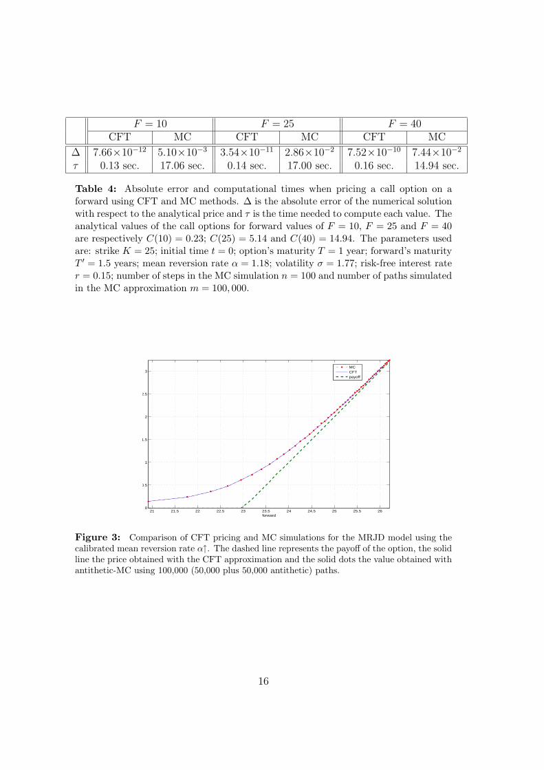
F = 10 F = 25 F = 40CFT MC CFT MC CFT MC

∆ 7.66×10−12 5.10×10−3 3.54×10−11 2.86×10−2 7.52×10−10 7.44×10−2

τ 0.13 sec. 17.06 sec. 0.14 sec. 17.00 sec. 0.16 sec. 14.94 sec.

Table 4: Absolute error and computational times when pricing a call option on aforward using CFT and MC methods. ∆ is the absolute error of the numerical solutionwith respect to the analytical price and τ is the time needed to compute each value. Theanalytical values of the call options for forward values of F = 10, F = 25 and F = 40are respectively C(10) = 0.23; C(25) = 5.14 and C(40) = 14.94. The parameters usedare: strike K = 25; initial time t = 0; option’s maturity T = 1 year; forward’s maturityT ′ = 1.5 years; mean reversion rate α = 1.18; volatility σ = 1.77; risk-free interest rater = 0.15; number of steps in the MC simulation n = 100 and number of paths simulatedin the MC approximation m = 100, 000.

21 21.5 22 22.5 23 23.5 24 24.5 25 25.5 260

0.5

1

1.5

2

2.5

3

forward

MCCFTpayoff

Figure 3: Comparison of CFT pricing and MC simulations for the MRJD model using thecalibrated mean reversion rate α↑. The dashed line represents the payoff of the option, the solidline the price obtained with the CFT approximation and the solid dots the value obtained withantithetic-MC using 100,000 (50,000 plus 50,000 antithetic) paths.

16

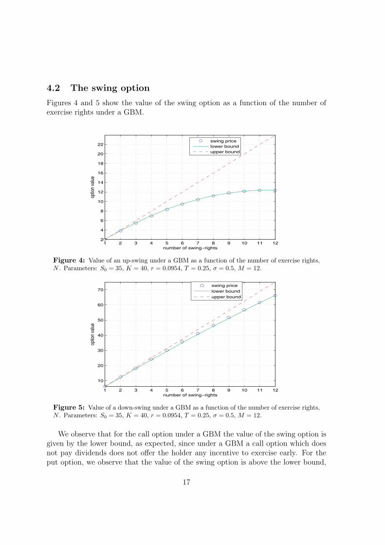
4.2 The swing option

Figures 4 and 5 show the value of the swing option as a function of the number ofexercise rights under a GBM.

1 2 3 4 5 6 7 8 9 10 11 122

4

6

8

10

12

14

16

18

20

22

number of swing−rights

optio

n va

lue

swing price

lower bound

upper bound

Figure 4: Value of an up-swing under a GBM as a function of the number of exercise rights,N . Parameters: S0 = 35, K = 40, r = 0.0954, T = 0.25, σ = 0.5, M = 12.

1 2 3 4 5 6 7 8 9 10 11 12

10

20

30

40

50

60

70

number of swing−rights

optio

n va

lue

swing price

lower bound

upper bound

Figure 5: Value of a down-swing under a GBM as a function of the number of exercise rights,N . Parameters: S0 = 35, K = 40, r = 0.0954, T = 0.25, σ = 0.5, M = 12.

We observe that for the call option under a GBM the value of the swing option isgiven by the lower bound, as expected, since under a GBM a call option which doesnot pay dividends does not offer the holder any incentive to exercise early. For theput option, we observe that the value of the swing option is above the lower bound,

17

and this value converges to the lower bound as we increase the number of exerciserights to the limit N = M , where as discussed by the second property in Section 3.1,we recover as the price of the swing the lower bound, i.e. the strip of 12 call options.

In Figures 6 and 7 we show the value of the swing options as a function of thenumber of exercise rights under the MRJD model.

1 2 3 4 5 6 7 8 9 10 11 12

10

20

30

40

50

60

70

80

90

100

110

number of swing−rights

optio

n va

lue

swing pricelower boundupper bound

Figure 6: Value of an up-swing option with strike price K = 18 under the calibrated MRJDmodel as a function of the number of exercise rights, N .

1 2 3 4 5 6 7 8 9 10 11 12

5

10

15

20

25

number of swing−rights

optio

n va

lue

swing pricelower boundupper bound

Figure 7: Value of a down-swing option with strike price K = 18 under the calibrated MRJDmodel as a function of the number of exercise rights, N .

For values of N < M we observe now that both the call and the put (the up/downswings) exhibit values which are clearly above the lower bound. The fact that we now

18

observe this premium above the lower bound is mainly attributed to the inclusion ofjumps in the model. Also as expected, for N = M the price of the swing convergesto the lower bound.

In Figure 8 we compare the price of the swing option for different number ofexercise rights under the MRJD model, the MRJD model with a lower mean reversionrate (α = 10 annualized) and a GBM with σ = 2.5 (which is the historical volatilityfor the entire data set we would use if we were to model using Black-Scholes). Forthe GBM the value of the swing option coincides with its lower bound, as discussedpreviously. For the MRJD model with both high and low mean reversion rate weobserve again that the swing option is clearly above the lower bound. However, forthe lower mean reversion rate the value of the swing option is higher, as would beexpected since the spot price reverts in a much longer time to its mean. For the caseN = M , both the GBM and the MRJD models converge to their lower bounds.

1 2 3 4 5 6 7 8 9 10 11 12

10

20

30

40

50

60

70

80

90

number of swing−rights

optio

n va

lue

GBMLB GBMlow MRJDlow LB MRJDMRJDLB MRJD

Figure 8: Value of an up-swing and its lower bound as a function of the number of exerciserights n under a GBM with volatility σ = 2.5, a MRJD model with lower mean reversion rate(α = 10 annualized) and the calibrated MRJD; K = 18.

Finally, we performed a sensitivity analysis with respect to the strike price K andthe number of exercise rights n. On Figure 9 we show a surface plot where the bottomsurface is the value of the lower bound and the top surface is the value of the swingoption. Examining this plot we can verify three properties. First, the value of theswing option is increasing with the number of exercise rights for the different valuesof K. Second, the value of the swing option tends to the lower bound on the limitN → M for every strike considered. Third, the value of the swing option increasesinversely with K; thus reflecting that a supplier selling this contract would offer thoseusers who are willing to be curtailed first (and therefore provide a lower strike price)

19

a higher discount on the forward.

12

34

56

78

910

1112

14

16

18

20

22

10

20

30

40

50

60

70

number of swing−rights

strike price

Figure 9: Value of an up-swing and its lower bound as a function of the number of exerciserights n and strike price K under the calibrated MRJD model. The bottom surface representsthe lower bound and the top surface the price of the swing option.

4.3 The discount on the forward

As we have discussed earlier, a supplier can replicate an interruption strategy byshorting a forward contract (covering a certain period of time) and longing an up-swing option which gives him the right to exercise N times, effectively cancelingthe obligation of supplying a unit of electricity when the option is exercised andcompensating the user with a pre-arranged shortage cost K. The consumer holds theopposite position on this portfolio, namely Πt = F T

t − Csw(St; K, T ). The up-swingoption in this portfolio clearly represents a net discount on the forward contractedfor that period from the consumer’s perspective. In Table 5, the second, fourth andsixth columns show respectively the value of the up-swing valued under three differentsettings: a GBM model, the presented MRJD but with a low level of mean reversionof α = 10 (annualized) and the MRJD model under the current calibration.14

The discounts shown are computed in each case with respect to a quoted forwardfor the period, which is Ft,T = 30MWh per day for daily delivery of one unit ofelectricity. As expected, the discount increases with the number of exercise rights,hence the customer who is willing to be interrupted more times will receive a highercompensation.

14For the GBM values in Table 5 and 6 we have used σ = 2.5, which is the resulting historicalvolatility from the entire data set we would use if we were to model with the Black-Scholes model.

20

n GBM discount MRJD (α↓) discount MRJD (α↑) discount1 10.0120 0.3708% 20.0583 0.7429% 9.7396 0.3607%2 19.6180 0.7266% 34.8036 1.2890% 15.3450 0.5683%3 28.8870 1.0699% 46.4124 1.7190% 19.6130 0.7264%4 37.7090 1.3966% 55.8967 2.0702% 23.0560 0.8539%5 46.2000 1.7111% 63.667 2.3580% 25.8360 0.9569%6 54.2950 2.0109% 70.1071 2.5966% 28.0580 1.0392%7 61.8830 2.2920% 75.657 2.8021% 29.8050 1.1039%8 68.9630 2.5542% 80.2259 2.9713% 31.0710 1.1508%9 75.4160 2.7932% 83.9911 3.1108% 31.9560 1.1836%10 81.1870 3.0069% 86.9844 3.2216% 32.5100 1.2041%11 86.1450 3.1906% 89.2961 3.3073% 32.7580 1.2133%12 89.9990 3.3333% 90.8624 3.3653% 32.8290 1.2159%

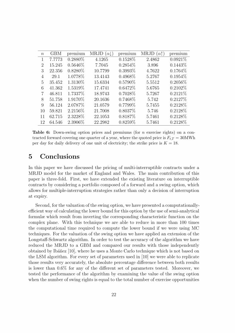
Table 5: Up-swing option prices and discounts (for n exercise rights) on a contractedforward covering one quarter of a year, where the quoted price is Ft,T = 30MWh perday for daily delivery of one unit of electricity; the strike price is K = 18.

As we can observe from this table, the discounts obtained with a MRJD modelwith lower mean reversion rate are higher than those obtained with a GBM, sincethe GBM does not incorporate any jumps. However, for a higher (and more realistic)level of mean reversion the price of the swing option decreases significantly, and thediscounts are approximately halved with respect to the other models. This showsthat the value of the swing option is sensitive to the estimation of the mean reversionrate.

As we have discussed earlier, we can also replicate an interruption strategy witha down-swing option by considering a consumer who owns a portfolio Π∗

t = F Tt +

P sw(St; K,T ). In this case the consumer will be prepared to pay a premium abovethe forward price in order to have the choice of exercising the down-swing option andtherefore selling back to the supplier a unit of electricity at a fixed price K, realizinga profit K − Sti , where ti is any of the chosen exercise dates.

In Table 6, the second, fourth and sixth columns show respectively the value ofthe down-swing valued under three different settings: a GBM model, the presentedMRJD but with a low level of mean reversion of α = 10 (annualized) and the MRJDmodel under the current calibration. The premiums shown are computed in each casewith respect to the quoted forward for the period, which is Ft,T = 30MWh per dayfor daily delivery of one unit of electricity. As we may observe from this table, thepremium increases with the number of exercise rights, as expected.

21

n GBM premium MRJD (α↓) premium MRJD (α↑) premium1 7.7773 0.2880% 4.1265 0.1528% 2.4862 0.0921%2 15.245 0.5646% 7.7045 0.2854% 3.896 0.1443%3 22.356 0.8280% 10.7799 0.3993% 4.7622 0.1764%4 29.1 1.0778% 13.4143 0.4968% 5.2767 0.1954%5 35.452 1.3130% 15.6334 0.5790% 5.5512 0.2056%6 41.362 1.5319% 17.4741 0.6472% 5.6765 0.2102%7 46.811 1.7337% 18.9743 0.7028% 5.7267 0.2121%8 51.758 1.9170% 20.1636 0.7468% 5.742 0.2127%9 56.124 2.0787% 21.0579 0.7799% 5.7455 0.2128%10 59.821 2.2156% 21.7008 0.8037% 5.746 0.2128%11 62.715 2.3228% 22.1053 0.8187% 5.7461 0.2128%12 64.546 2.3906% 22.2982 0.8259% 5.7461 0.2128%

Table 6: Down-swing option prices and premiums (for n exercise rights) on a con-tracted forward covering one quarter of a year, where the quoted price is Ft,T = 30MWhper day for daily delivery of one unit of electricity; the strike price is K = 18.

5 Conclusions

In this paper we have discussed the pricing of multi-interruptible contracts under aMRJD model for the market of England and Wales. The main contribution of thispaper is three-fold. First, we have extended the existing literature on interruptiblecontracts by considering a portfolio composed of a forward and a swing option, whichallows for multiple-interruption strategies rather than only a decision of interruptionat expiry.

Second, for the valuation of the swing option, we have presented a computationally-efficient way of calculating the lower bound for this option by the use of semi-analyticalformulæ which result from inverting the corresponding characteristic function on thecomplex plane. With this technique we are able to reduce in more than 100 timesthe computational time required to compute the lower bound if we were using MCtechniques. For the valuation of the swing option we have applied an extension of theLongstaff-Schwartz algorithm. In order to test the accuracy of the algorithm we havereduced the MRJD to a GBM and compared our results with those independentlyobtained by Ibanez [10], where he uses a Monte Carlo technique which is not based onthe LSM algorithm. For every set of parameters used in [10] we were able to replicatethose results very accurately, the absolute percentage difference between both resultsis lower than 0.6% for any of the different set of parameters tested. Moreover, wetested the performance of the algorithm by examining the value of the swing optionwhen the number of swing rights is equal to the total number of exercise opportunities

22

(the case N = M). For the different cases considered it has been shown that the valueof the swing option converges convexly as N→M to its lower bound, as expected.

Third, we have also discussed and priced down-swing options which enable us toreplicate a multi-interruption strategy by transferring the decision of interruption tothe user which would enable large users or retailers to benefit from sudden falls onthe price of electricity.

The results on the discounts (and premiums for the down-swing) reflect that theseare increasing with the number of rights, as one would expect, since the owner of theoption has greater flexibility. We have also considered the sensitivity of the valuationwith respect to the mean reversion rate and the strike price for the contract. Ourresults confirm that the value of the swing option decreases with increasing meanreversion rate and increases with decreasing strike price, as expected.

Finally, the values of the discounts and premiums obtained with the calibratedMRJD model are relevant, specially considering that the current valuation has beenperformed for delivery of a single unit of electricity. When taking into account thelarge volumes typically traded, the discounts may prove a real incentive for marketparticipants to enter into these contracts.

23

A Proof of Proposition 2.1

Noting that −α(T ′ − t) = α(T − T ′)− α(T − t), we can rewrite (3) as

F T ′t = e(xt−gt)e−α(T−t)

︸ ︷︷ ︸Ω

eeα(T−T ′)eg(T ′)−λ

R T ′t σse−α(T ′−s)ds+ 1

2

R T ′t σ2

se−2α(T ′−s)ds+R T ′

t Φ(s)lds.

(A 1)Now, solving for Ω from (2) and noting that the integrals in (3) can be written as∫ T ′

tf(·)ds =

∫ T

tf(·)ds +

∫ T ′

Tf(·)ds we obtain after rearranging some terms

F T ′t = eg(T ′)+(xT−gT )e−α(T ′−T )−λ

R T ′T σse−α(T ′−s)ds+ 1

2

R T ′T σ2

se−2α(T ′−s)ds+R T ′

T Φ(s)lds

× e12

R Tt σ2

se−2α(T ′−s)ds+R T

t Φ(s)lds−R Tt σ2

se−α(T ′−s)dZs−R T

t e−α(T ′−s) ln Jsdqs . (A 2)

Finally, noting from (3) that the first line of (A 2) is precisely F T ′T , we may finally

write the forward at time T maturing at time T ′ conditional on the forward at timet maturing at time T ′, this is

F T ′T = F T ′

t e−12

R Tt σ2

se−2α(T ′−s)ds−R Tt Φ(s)lds+

R Tt σ2

se−α(T ′−s)dZs+R T

t e−α(T ′−s) ln Jsdqs . (A 3)

We then calculate the characteristic function as Ψ(ξ) := Et

[e−iξ ln F T ′

T

]to arrive

after some calculations to (7b).

We now need to transform the payoff of the option and study the region of analyt-icity of the integrand. These two issues are addressed in the following sub-sections.

A.1 Transforming the payoff of a European Call

The CFT of a function f(x) can be defined as

f(ξ) =

∫ ∞

−∞eiξxf(x) dx = L [f(x)] , (A 4)

where ξ = a + ib and a, b ∈ R.

Likewise, the inverse CFT can be defined as

f(x) =1

2π

∫ ∞+ib

−∞+ib

e−iξxf(ξ) dξ. (A 5)

The payoff of a European call option written on an underlying Ft is given by

C (FT , T ) =

FT −K if FT ≥ K

0 if FT < 0.(A 6)

24

By substituting xt = ln Ft we may write

C (xT , T ) =

exT −K if xT ≥ ln K

0 if xT < ln K.(A 7)

Applying (A 4) and integrating we obtain

L [C (x, T )] =

∫ ∞

−∞eiξx max (ex −K, 0) dx

=

(ex(1+iξ)

1 + iξ− Keiξx

iξ

)∣∣∣∣∞

ln(K)

= limx→∞

(ex(1+iξ)

1 + iξ− Keiξx

iξ

)−

(eln(K)(1+iξ)

1 + iξ− Keiξ ln(K)

iξ

). (A 8)

Clearly the first term in the last equation diverges unless we require that ξIm > 1.Hence, since we have defined ξ = a + ib, we must restrict b > 1, assuring the Fouriertransform of the payoff exists.

Hence, we may finally write

L [C (xT , T )] =−K1+iξ

ξ2 − iξ, for b > 1. (A 9)

A.2 Strip of Regularity

When defining the CFT and its inverse in (A 4) and (A 5) we have not yet saidanything about the conditions under which the CFT can be applied.

Following Dettman [5], let us consider any f(x) continuous and with piecewisecontinuous first derivative in any finite interval.

Let f(x) = O(eζx) as x → ∞ and f(x) = O(eθx) as x → −∞. Then there existsnumbers M, N and R such that the following holds

|f(x)| ≤

Meζx if x ≥ RNeθx if x ≤ −R,

(A 10)

where M , N and R > 0.

We can rewrite (A 4) as

f(ξ) =

∫ −R

−∞eiξxf(x) dx +

∫ R

−R

eiξxf(x) dx +

∫ ∞

R

eiξxf(x) dx (A 11)

25

and using Cauchy’s inequality together with (A 10) we have∣∣∣∣∫ −R

−∞eiξxf(x) dx

∣∣∣∣ ≤ N

∫ −R

−∞

∣∣eiξx∣∣ eθx dx;

≤ N

∫ −R

−∞e(θ−b)x dx

=N

θ − b

(e−R(θ−b) − lim

x→−∞e(θ−b)x

). (A 12)

Clearly (A 12) only exists if θ − b > 0 ⇔ b < θ.

Likewise, ∣∣∣∣∫ ∞

R

eiξxf(x) dx

∣∣∣∣ ≤ M

∫ ∞

R

ex(ζ−b) dx, (A 13)

which only exists if ζ − b < 0 ⇔ b > ζ. Thus, the CFT, as defined in (A 4) is welldefined when ζ < b < θ.

Under rather general conditions for a function f(ξ), the inverse transform can becomputed by integrating along any line parallel to the real axis lying in the strip ofanalyticity of f(ξ),

1

2π

∫ ∞+ib1

−∞+ib1

e−iξxφ(ξ) dξ =1

2π

∫ ∞+ib2

−∞+ib2

e−iξxφ(ξ) dξ, (A 14)

where b1 and b2 are any real numbers between ζ and θ.

This last equation can be easily proved by applying Cauchy’s theorem in a rect-angular contour lying between ζ and θ, of horizontal sides b1, b2 and vertical sidesT,−T , and taking the limit as T →∞.

Cauchy’s theorem states that∮

Cf(ξ) dξ = 0, if the integral is taken along a curve

which encloses positively an analytical region. The integral cancels on the sides ofthe rectangle in the limit T → ±∞, and since C = C1 + C2 + C3 + C4 we are leftwith

∫C1 f(ξ) dξ =

∫C3 f(ξ) dξ, which is (A 14).

According to Lewis [15], it can be shown that for most examples involving optionpricing, ζ < 0 and θ > 1. Furthermore, as we have seen in (A 9) the transformedpayoff is well defined for values of b > 1.

Hence, having shown that the CFT and its inverse are well defined in the stripA = b: ζ < b < θ, and that b > 1 for a European call option, we price in the stripdefined by b s.t. max(1, ζ) < b < θ.

2

26

References

[1] Alvaro Cartea and Marcelo G. Figueroa. Pricing in Electricity Markets: a MeanReverting Jump Diffusion Model with Seasonality. Applied Mathematical Fi-nance, 12(4):313–335, December 2005.

[2] Alvaro Escribano, Juan Ignacio Pena, and Pablo Villaplana. Modelling electricityprices: International evidence. Universidad Carlos III de Madrid – working paper02-27, June 2002.

[3] Fred Espen Benth and Steen Koekebakker. Stochastic Modeling of FinancialElectricity Contracts. Dept. of Math. University of Oslo, ISSN 0806-2439(24),2005.

[4] Alan Brechner, Alvaro Cartea, and Marcelo G. Figueroa. A Study of the MarketPrice of Risk in Wholesale Electricity Markets: the Nord Pool Case. Birkbeck,University of London, working paper.

[5] John W. Dettman. Mathematical Methods in Physics and Engineering. DoverPublications, 1998.

[6] Uwe Dor. Valuation of Swing Options and Examination of Exercise Strategies byMonte Carlo Techniques. MSc. Thesis, University of Oxford, September 2003.

[7] Thomas W. Gedra. Optional Forward Contracts for Electric Power Markets.IEEE Transactions on Power Systems, 9(4):1766–1773, November 1994.

[8] Helyette Geman and Andrea Roncoroni. Understanding the Fine Structure ofElectricity Prices. The Journal of Business, 79(5), 2006.

[9] Paul Glasserman. Monte Carlo Methods in Financial Engineering. Springer,2004.

[10] Alfredo Ibanez. Valuation by Simulation of Contingent Claims with MultipleEarly Exercise Opportunities. Mahtematical Finance, 14(2):223–248, April 2004.

[11] Alfredo Ibanez and Fernando Zapatero. Monte Carlo Valuation of AmericanOptions through Computation of the Optimal Exercise Frontier. Journal ofFinancial and Quantitative Analysis, 39(2), June 2004.

[12] Patrick Jaillet, Ehud I. Ronn, and Stathis Tompaidis. Valuation of Commodity-Based Swing Options. Management Science, 50(7):909–921, July 2004.

27

[13] Rajnish Kamat and Shmuel S. Oren. Exotic Options for Interruptible Electric-ity Supply Contracts. Operations Research, 50(5):835–850, September-October2002.

[14] Steven G. Kou. A Jump-Diffusion Model for Option Pricing. Management Sci-ence, 48(8):1086–1101, August 2002.

[15] Alan L. Lewis. Option Valuation Under Stochastic Volatility. Finance Press,2000.

[16] Alan L. Lewis. A Simple Option Formula for General Jump-Diffusion and OtherExponential Levy Processes. Envision Financial Systems and OptionCity.net,September 2001.

[17] Francis A. Longstaff and Eduardo S. Schwartz. Valuing American Options bySimulation: a Simple Least-Squares Approach. The Review of Financial Studies,14(1):113–147, Spring 2001.

[18] Eduardo S. Schwartz. The Stochastic Behavior of Commodity Prices: Implica-tions for Valuation and Hedging. The Journal of Finance, 52(3):923–973, July1997.

[19] Eduardo S. Schwartz and James E. Smith. Short-term Variations and Long-termDynamics in Commodity Prices. Management Science, 46(7):893–911, July 2000.

28