A Conceptual Framework for Estimating the Impact of Climatic Uncertainty and Shocks on Land Use,...

DLSU Business & Economics Review 24.2 (2015), pp. 13-31

Copyright © 2015 by De La Salle University, Manila, Philippines

A Conceptual Framework for Estimating the Impact of Climatic Uncertainty and Shocks on Land Use, Food Production, and Poverty in the PhilippinesCaesar CororatonVirginia Polytechnic Institute and State [email protected]

Arlene InocencioDe La Salle University, Manila, Philippines

Anna Bella Siriban-ManalangDe La Salle University, Manila, Philippines

Marites TiongcoDe La Salle University, Manila, Philippines

Wide variations in climatic conditions from prolonged dry season to frequent occurrence of super typhoons have significant impact on the Philippines, especially on rural poor households which depend heavily on agriculture and food production for subsistence and income. This paper provides a research framework that can be used to understand the dynamics between climate change and agriculture. The framework incorporates the effects of climate change on agricultural productivity, as well as the effects of agricultural activities and land use on climate change through the emission of greenhouse gasses. The framework uses three simulation models to analyse the impact of climate change: a global CGE model, a Philippine CGE model, and a Philippine poverty microsimulation model.

JEL Classifications: C68, D58, Q540, O130

Keywords: Climate change, CGE, land use, food security, food production, Philippines

14 VOL. 24 NO. 2DLSU BUSINESS & ECONOMICS REVIEW

INTRODUCTION

A majority of poor households in rural Philippines depend on cultivation of crops and on raising of livestock and catching of fish for subsistence and for income. These agricultural activities are highly vulnerable to extreme and erratic changes in climatic conditions. Long duration of droughts diminishes soil fertility. Intense rainfall and flood increase soil erosion and reduce the area for crop cultivation. In coastal communities, climate change increases groundwater and estuary contamination by saltwater incursion, typhoon surges, heat stress, and droughts. A rise in the sea level leaves salt on soils, rendering some areas unsuitable for agriculture. The impact on agriculture and food production is significant because over 80% of global agriculture is rainfed. Climate change also affects agriculture infrastructure. Typhoon damages equipment for food production and critical agricultural infrastructure such as farm-to-market roads, railways, and vehicles. Climate change can also cause more pests and diseases as the natural biota in an area is altered (Gornall et al., 2010). All this affects agricultural productivity, food production, and supply.

Adaptation to climate change involves technologies to improve irrigation systems and varieties of seed through selective breeding or through genetic modification. The impact of climate change on agriculture can also be mitigated through proper crop management, livestock and pasture management, and reduction in the transport of agriculture products (Lin, Chappell, Vandermeer, Smith, Quintero, Bezner-Kerr, ..., & Perfecto, 2012). However, while these measures have somewhat alleviated the challenges posed by climate change, erratic weather conditions still remain a major factor affecting agricultural productivity and production. Research results have shown that without sufficient adaptation measures, climate change projections for 2030 (for 12 food insecure

regions) indicate that South Asia and Southern Africa will likely experience severe impacts on crop production. Maize, wheat, and rice top the list of crops which production are most severely affected (Lobell, Burke, Tebaldi, Mastrandrea, Falcon, & Naylor, 2008).

However, while climate change affects agriculture and food production and livelihood of rural households, agriculture activities and changes in land use affect the global climate regimes primarily through the production and the release of greenhouse gases (GHG) such as methane, carbon dioxide, and nitrous oxide. Change in land use from forests to fields for agriculture activities causes deforestation and desertification that alters the earth’s ability to absorb and reflect heat and light. This affects global temperatures (Intergovernmental Panel on Climate Change, 2007). However, the contribution of agriculture systems to climate change is not uniform across sectors. For example, industrial agriculture contributes significantly to global warming because of higher GHG emissions than farm activities. The small-scale farms use less energy and release fewer GHG.

Land use involves management and modification of natural environment or wilderness into crop fields, pastures, and settlements. The Food and Agricultural Organization (FAO) (FAO, 1996; Gregorio, 2005) defined land use as “…characterized by the arrangements, activities and inputs people undertake in a certain land cover type to produce, change, or maintain it.” FAO has standardized the classification of the types of land use into three categories: (i) agriculture, (ii) forestry, and (iii) other land. In the Philippines, the National Statistics Coordination Board (NSCB) (2010) classifies Philippine land into five categories: (1) alienable and disposable Land, (2) total forest land, (3) national parks, (4) civil reservation, and (5) fishpond development. To be consistent with international standards, the proposed framework merges the land use types

A CONCEPTUAL FRAMEWORK CORORATON, C., ET AL 15

provided by the NSCB to fit those defined by the FAO. That is, types (1) and (5) under NSCB fall under agriculture; type (2) falls under forestry; and types (3) and (4) fall under Other Land.

It is difficult to quantify the effects of agriculture activities and changes in land use changes to climate change. However, there are a few methods and models that have recently been developed to study effect of changes in land use on climate change (Turner, Lambin, & Reenberg, 2007). Models which build scenarios that involve both the impact and contribution of agriculture to climate change are among the next-generation scenarios that challenge climate change research (Moss, Edmonds, Hibbard, Manning, Rose, van Vuuren,…, Wilbanks, 2010). These models combine an understanding of the variability in earth’s climate system, its response to human and natural influences, and the effect of changes on the populations.

Land use is driven by both socioeconomic and biophysical factors such as population and economic growth and increasing demand for energy. It is critical to understand the interaction between climate and land use, and how it influences future climate and land use predictions, and consequently food supply. In this framework paper, we propose to examine the impacts of changes in anthropogenic GHG concentrations and land use on regional climate, and the impacts of climate changes and socioeconomic factors on land use. The proposed work utilizes the modelling framework of Wang, Kockelman, and Wang (2011) that incorporates both the biophysical and socioeconomic drivers for land use into a regional climate system model. In particular, the model focuses on the impact of land use and the natural vegetation dynamics, that is, the response of natural vegetation to predicted climate changes and the resulting climate feedback. These have economy-wide effects which are analysed using a global computable general equilibrium model (CGE). The impact of climate change on sectoral productivity,

production and demand for commodities, commodity prices, factor demand and factor prices, and household income is analysed through the Philippine CGE model. The impact on poverty is analysed using a poverty micro simulation model that uses data from family income and expenditure survey. The proposed research focuses on the Philippines.

REVIEW OF LITERATURE

Climate Change and Agriculture

Climate change presents a major challenge to agriculture. Based on the 2011 Asian Development Bank (ADB) report, “excess heat and drought in some places, and oversaturation of soil and physical damage from increased rainfall in others can likely result in crop losses and lower livestock and poultry production” (p. viii).

Vermeulen, Aggarwal, Ainslie, Angelone, Campbell, Challinor, …, Wollenberg (2010) found strong evidence that worsening climate change exacerbates poverty and food insecurity. Future impacts of climate change on livestock production are both direct (e.g., productivity losses due to physiological stress, owing to increasing temperature) and indirect (e.g., changes in the availability, quality and prices of inputs such as fodder, energy, disease management, housing and water). In aquaculture, the distribution and population sizes of marine fish species are affected by changes in sea temperature. Climate change also affects fishers due to its impact on habitats, stocks, and distribution of key fish. Changes in global temperatures disrupt the normal structure of ecosystems. The impacts of climate change on the structure and function of plant and animal communities are widely demonstrated for terrestrial, freshwater and marine ecosystems. Changes in species distributions, phenology, and ecological interactions have impacts on


pollination, invasions of agricultural systems by weeds, and locations of major marine fishing grounds. These changes in the ecosystems lead to spawning of newer and more persistent pests and diseases. There is growing evidence that climatic variations have are already influenced the distribution and virulence of crop pests and diseases.1

Vermeulen et al. (2010) also found that climate change has significant impacts on the emergence, spread, and distribution of livestock diseases through various pathways. There is evidence that carbon fertilization adversely affects agriculture. There is an ongoing debate about the impacts of carbon fertilization on plants and yields, and how changing ozone concentrations may interact with carbon dioxide effects and with other biotic and abiotic stresses. However, the impact is observed in grassland productivity and in species composition and dynamics, which resulted in changes in animal diets and reduced nutrient availability for animals. Climate change poses dire consequences on fresh water supply globally for drinking and for irrigation. Climate change also impacts the delivery and effectiveness of irrigation. The predicted increase in precipitation variability, coupled with higher evapotranspiration under hotter mean temperatures, implies longer drought periods that increase irrigation requirements, even if the total precipitation during the growing season remain constant. Furthermore, climatic fluctuations are known to affect post-harvest losses and food safety during storage, for example by causing changes in populations of aflatoxin-producing fungi. It is anticipated that more frequent extreme weather events under climate change will damage infrastructure, with detrimental impacts on food storage and distribution, to which the poor is most vulnerable. Finally, prices of most cereals will rise significantly due to climatic changes leading to a fall in consumption and hence decreased calorie availability and increased child malnutrition. Furthermore, research indicates that

the nutritional value of food, especially cereals, is also affected by climate change. Climate change also affect the ability of individuals to use food effectively by altering the conditions for food safety and changing the disease pressure from vector, water, and food-borne diseases.

Butt, McCarl, Angerer, Dyke, and Stuth (2005) predicted that changes in climate result in changes in crop yield from -17% to +6% at national level. Simultaneously, forage yields fall by 5% to 36% and livestock animal weights are reduced by 14% to 16%. The economic losses range between US$70 million and US$142 million, with producers gaining and consumers losing. The percentage of population found to be at risk of hunger rises from a current estimate of 34% to an after climate change level of 64% to 72%. Nelson, G.C., Rosegrant, M. W., Koo, J., Robertson, R., Sulser, T., Zhu, T., …, Lee, D. (2009) predicted that climate change results in additional price increases for the most important agricultural crops such as rice, wheat, maize, and soybeans. Under a no climate change scenario, world prices for the most important agricultural crops increase between 2000 and 2050 because of population and income growth and biofuels demand. The price of rice increases by 62%, maize by 63%, soybeans by 72%, and wheat by 39%. Under a scenario with climate change, there are additional increases in prices of these commodities (32% to 37% for rice; 52% to 55% for maize; 94% to 111% for wheat, and 11% to 14% for soybeans). Irrigated wheat and irrigated rice are hard hit by climate change. In developing countries crops without CO2 fertilization experience declining yields. On average, yields in developed countries are affected less than those in developing countries.

Increasing feed prices result in higher meat prices. Higher prices reduce the growth of meat consumption and decrease cereal consumption. Calorie availability in 2050 is not only lower than in the no climate change scenario, it is lower relative to 2000 levels throughout the developing


world. For the average consumer in a developing country, calorie availability in 2050 is lower by 7% relative to 2000. By 2050, the decline in calorie availability increases child malnutrition by 20% relative to a world with no climate change. Climate change eliminates much of the improvement in child malnourishment levels that would have occurred under a no climate change scenario. Thus, aggressive agricultural productivity investments of US$7.1 million to US$7.3 billion are needed to raise calorie consumption enough to offset the negative impacts of climate change on the health and well-being of children.

Simulation Models

One of the simulation models used to examine the dynamics between climate change and agriculture is CGE. This type of model is used because it captures the economy-wide effects of climate change from commodity supply and prices, factor demand and prices, to household income and consumption. The model also captures the effects across sectors of the economy.

In the literature, several CGE models are linked with partial equilibrium models to better capture the climate change-agriculture dynamics. The Integrated Assessment Model (IAM) is an example where a CGE model is linked with a partial equilibrium agricultural model for land-use model (Palatnik & Roson, 2009). The IAM model contains detailed representation of the different economic processes. However, one drawback of IAM is that the integration of the CGE in model is not consistent with the partial equilibrium, thus convergence of the two is not always assured. he CGE and the partial equilibrium models use different assumptions, data sources, data, and units of measurements. Adjustments in the CGE parameters are necessary for model convergence. Applying the necessary adjustments in the CGE parameters, Ronneberger, Berrittella, Bosello and

Tol (2009) showed that changes in emissions and crop production move in the same direction as changes in GDP and welfare. Changes in trade balance and crop prices move in the opposite direction. The simulations demonstrate that crop production adjusts according to the pattern of induced yield changes brought about by climate change. Higher yield increases crop production while lower yield decreases production. Any yield losses are compensated by increasing the area used for production which increases prices, negatively affects the balance of trade, and decreases GDP and welfare. Furthermore, the model simulation shows that climate change has a negative impact on GDP and welfare for most regions except for Central America and South Asia, and sub-Saharan Africa, Canada, and Western Europe; the former group with stronger gains and the latter group with smaller gains.

Zhai, Lin and Byambadorj (2009) assessed the long-term impacts of climate change on agricultural production and trade in China using a global CGE. They found that climate change results in a 1.3% decline in GDP and a welfare loss of 1.1% by 2080. China’s agricultural productivity declines, which increases the country’s dependence on world agricultural markets. This effect leads to additional losses in welfare and output through unfavorable terms-of-trade effects. China’s food processing sectors are negatively affected by the decline in agricultural productivity as well as the decline in global agricultural productivity as a result of climate change.

Zhai and Zhuang (2009) employed a CGE model to assess the economic effects of climate change for Southeast Asian countries through 2080. The simulation results suggest that global crop production decreases by 7.4%. There is uneven distribution of productivity losses across the different regions, with higher decline in developing countries. A reduction in global agricultural productivity has non-negligible negative impacts on Southeast Asia. With lower


agricultural productivity, the dependence of Southeast Asia on crop imports increases, causing welfare losses. The negative effects are lower in Singapore and Malaysia, but higher in Indonesia, Thailand, Vietnam, and the Philippines. GDP in the last three countries contracts by 1.7% to 2.4%.

Golub, Hertel and Sohngen (2009) divided the earth into agroecological zone (AEZ) and employed a global model with land allocation mechanism to study the effects of land use change on greenhouse gas emissions.2 The study demonstrates that as population and per capita income increase and consumption patterns change, the strongest growth in consumer demand is predicted in the forestry sector due to the increased demand for furniture, housing, and paper products. At the same time, unmanaged forest lands are converted to production lands in all regions except in places where no unmanaged forests are available. In Australia, New Zealand, North America, Latin America, and Western Europe, land used in forestry production declines while that for agriculture expands. Within the agricultural sector in these regions, more land is used for crops while less is used for livestock production. In the rest of the regions, including Southeast Asia and South Asia, land employed in commercial forestry expands while that for agriculture contracts as a response to increased demands for forest-based products worldwide.

Research that looks at the effects of climate change on poverty supplements the CGE model with poverty microsimulation models that use detailed household data from household surveys. The CGE model accounts for the impact of climate change on macro variables such as agricultural productivity and production, commodity demand and prices factor demand and factor returns, and household income. This set of information is used to change the distribution of household income in household surveys. There are several poverty simulation models available in the literature such as the Global Income Distribution Dynamics (GIDD) of the World

Bank (de Hoyos, 2008; Estrades 2013; Cockburn, 2001; Cororaton & Corong, 2009).

Framework of Analysis

To understand the dynamics between climate change and agriculture in the Philippines, the paper proposes a modelling framework that can be used to assess the impacts of climate change and land use patterns on crop yields and food production, and future land uses and emissions of greenhouse gases. The framework assumes that land use and changes in land cover are factors which exacerbate greenhouse gases that induce climate change. In turn, climate change is an important driver of changes in land use and land cover. This feedback affects several critical socio-economic factors especially in rural areas, which further drive changes in future land use. The modelling framework adopted is from Wang, Zhang, Pal, You (2011) and shown in Figure 1.

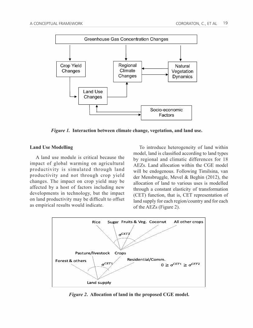
In most studies, land use predictions have not considered the effects of climate change. Land use and natural vegetation dynamics are not taken into account in most research work on climate change predictions. In Figure 1, changes in the concentration of greenhouse gases affect crop yields, climate changes at specific regions, and natural vegetation in those regions. Changes in crop yields affect the degree of utilization of land to various uses. The utilization of land to various uses is also affected by socio-economic factors (such as changes in market policies, poverty and income distribution, population growth, etc.). Changes in the utilization of land have feedback effects on the emission of greenhouse gases, which in turn affect the concentration of these gases that affect future climate change patterns. Thus, prediction of future climate is more than just a prediction of greenhouse gas emissions and its resulting climatic response. Land use and cover changes are considered in the framework to have significant climatic influence.


Land Use Modelling

A land use module is critical because the impact of global warming on agricultural productivity is simulated through land productivity and not through crop yield changes. The impact on crop yield may be affected by a host of factors including new developments in technology, but the impact on land productivity may be difficult to offset as empirical results would indicate.

To introduce heterogeneity of land within model, land is classified according to land types by regional and climatic differences for 18 AEZs. Land allocation within the CGE model will be endogenous. Following Timilsina, van der Mensbruggle, Mevel & Beghin (2012), the allocation of land to various uses is modelled through a constant elasticity of transformation (CET) function, that is, CET representation of land supply for each region/country and for each of the AEZs (Figure 2).

Figure 1. Interaction between climate change, vegetation, and land use.

Figure 2. Allocation of land in the proposed CGE model.


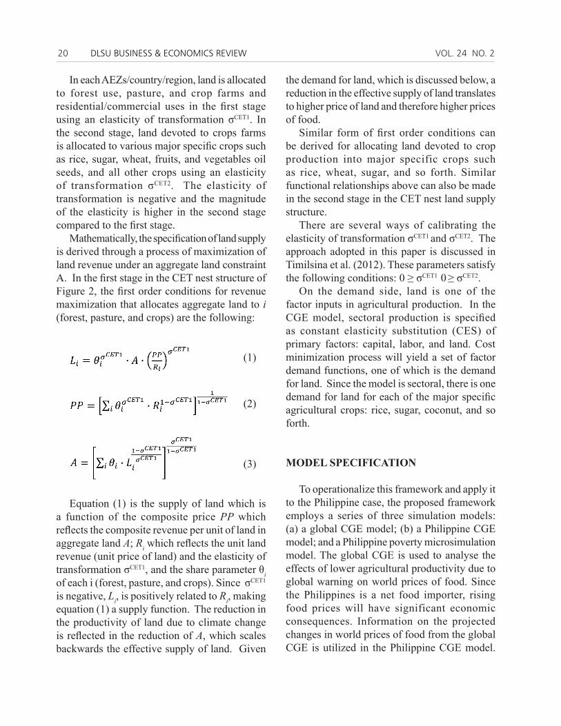
In each AEZs/country/region, land is allocated to forest use, pasture, and crop farms and residential/commercial uses in the first stage using an elasticity of transformation σCET1. In the second stage, land devoted to crops farms is allocated to various major specific crops such as rice, sugar, wheat, fruits, and vegetables oil seeds, and all other crops using an elasticity of transformation σCET2. The elasticity of transformation is negative and the magnitude of the elasticity is higher in the second stage compared to the first stage.

Mathematically, the specification of land supply is derived through a process of maximization of land revenue under an aggregate land constraint A. In the first stage in the CET nest structure of Figure 2, the first order conditions for revenue maximization that allocates aggregate land to i (forest, pasture, and crops) are the following:

(1)

(2)

(3)

Equation (1) is the supply of land which is a function of the composite price PP which reflects the composite revenue per unit of land in aggregate land A; Ri which reflects the unit land revenue (unit price of land) and the elasticity of transformation σCET1, and the share parameter θi of each i (forest, pasture, and crops). Since σCET1

is negative, Li, is positively related to Ri, making equation (1) a supply function. The reduction in the productivity of land due to climate change is reflected in the reduction of A, which scales backwards the effective supply of land. Given

the demand for land, which is discussed below, a reduction in the effective supply of land translates to higher price of land and therefore higher prices of food.

Similar form of first order conditions can be derived for allocating land devoted to crop production into major specific crops such as rice, wheat, sugar, and so forth. Similar functional relationships above can also be made in the second stage in the CET nest land supply structure.

There are several ways of calibrating the elasticity of transformation σCET1 and σCET2. The approach adopted in this paper is discussed in Timilsina et al. (2012). These parameters satisfy the following conditions: 0 ≥ σCET1 0 ≥ σCET2.

On the demand side, land is one of the factor inputs in agricultural production. In the CGE model, sectoral production is specified as constant elasticity substitution (CES) of primary factors: capital, labor, and land. Cost minimization process will yield a set of factor demand functions, one of which is the demand for land. Since the model is sectoral, there is one demand for land for each of the major specific agricultural crops: rice, sugar, coconut, and so forth.

MODEL SPECIFICATION

To operationalize this framework and apply it to the Philippine case, the proposed framework employs a series of three simulation models: (a) a global CGE model; (b) a Philippine CGE model; and a Philippine poverty microsimulation model. The global CGE is used to analyse the effects of lower agricultural productivity due to global warning on world prices of food. Since the Philippines is a net food importer, rising food prices will have significant economic consequences. Information on the projected changes in world prices of food from the global CGE is utilized in the Philippine CGE model.


The results on the allocation of land to various uses from the global CGE model are applied to the Philippine CGE model. The poverty microsimulation model uses these results to change the distribution of household income in the family income and household survey to calculate the effects on poverty in the Philippines.

Global CGE Model

The specification of the global CGE model is discussed in detail in Cororaton and Orden (2014). The model specification combines key structural features of two global CGE models: (a) the global model of the Partnership for Economic Policy (PEP); and (b) the global model of the World Bank (van der Mensbrugghe, 2008). The model is calibrated to GTAP 8 database, which comprises 57 commodities in 129 countries. The model includes two types of labor (skilled and unskilled), capital, land, and natural resources.

Production. The production sector of the model has a three-level structure. At the first level, sectoral output is produced using value added and aggregate intermediate consumption using a set of fixed coefficients. At the second level, the aggregate intermediate consumption is broken down into intermediate demand for goods and services using another set of fixed coefficients. Also at the second level, sectoral value added is specified as a constant elasticity of substitution (CES) function of composite capital and composite labor. At the third level, composite labor is specified as a CES function of two types of labor (skilled and unskilled). Also at the third level, composite capital is specified as a CES function of three types of capital: physical capital, land, and natural resources.

Household. There is only one household in each country/region in the model. This household earns income from earnings from the two types of labor and the two types of capital. It pays income tax. Its household savings is a linear

function of its disposable income. Its household demand for goods and service is specified as a linear expenditure system (LES).

Government. In each country/region, the government earns its revenue from income taxes, indirect taxes on commodities, taxes on the use of capital and labor in each sector, import tariffs, export taxes, and production taxes. Government savings is determined as the difference between total government revenue and total government expenditure. Total government expenditure is distributed among commodities using a set of fixed shares. For a given amount of government expenditure budget, the quantity demanded for each commodity varies inversely with the price of the commodity.

Investment. In the model, investment expenditure (gross fixed capital formation, GFCF) in each country/region is constrained by the savings-investment equilibrium. GFCF is distributed among commodities using a set of fixed shares. For a given amount of investment expenditure, the quantity demanded for each commodity for investment purposes varies inversely with the price of the commodity.

Exports. In each sector, the producer allocates output to three market outlets so as to maximize sales revenue for a given set of prices in these markets. These outlets are: domestic market, export market, and international transport margin services. Imperfect substitutability is assumed among products sold in these outlets by means of a CET aggregator function. Sales revenue maximization by the producer given a set of prices will result in a supply function in each of the outlets: supply to the domestic market, supply to the export market, and supply to the international transport margin services.

Export of each commodity is further disaggregated using another CET function to the various export destinations, which also implies imperfect substitutability among exports to these destinations. The producer maximizes its export revenue for a given set of export prices. This will


result in a supply function of each commodity in each export destination.

Domestic Demand. The goods and services available in the domestic market consist of those that are domestically produced and imports. In the model, domestically produced and imported goods are imperfect substitutes and are differentiated by prices. This product differentiation is through a CES function. The prices of domestically produced goods include indirect taxes. The prices of imported goods include import tariffs, international transport margins, and indirect taxes. Cost minimization of buying these goods given a set of prices will result in demand functions for domestically produced goods and imports.

Imports. Imports of each commodity are further disaggregated using another CES function to the various sources of imports or import origin, which also implies product differentiation among imports from the various origins. Cost minimization given a set of prices will result in demand functions for imports in each of the import origins.

External Account. In the GTAP 8 database, information is available on the amount of trade margin in each sector associated with each bilateral trade flows between countries/regions. However, there is no information available matching the producers of the international transport margin services to the individual bilateral trade flows. Therefore, disaggregating the international transport margin services similar to the breaking down of exports of goods and services to the various export destinations may not be possible as there is no information available in the GTAP 8 database needed to calibrate this part. Thus in the model, the supply of international transport margin services in each country/region is pooled in “external account (EA),” and its production is shared among suppliers in each country/region through a competitive process. Furthermore, this EA vis-à-vis each country/region includes payments for the value of the country’s/region’s

imports including international transport margins. The expenditure in the EA consists of the value of exports, including international margins. The difference between revenue and expenditure in the EA is foreign savings. The negative of foreign savings is the current account balance of each country/region.

Prices and Mark-Ups. The model has a system of prices that reflects the cost of production plus a series of mark-ups which consists of layers of taxes and international transport margins. The model has a unique price vector that clears the market for goods and services and the market for factors of production.

Model Closure. The details of the model closure is given in Appendix A. Some of its features include fixing the following variables: nominal exchange rate, real government expenditure, government investment demand, supply of factors of production in each period, and current account balance. The numeraire of the model is the GDP deflator of a reference country/region.

Model Dynamics. The model is dynamic-recursive. The model links one period to the next using two types of equations. One equation updates exogenous variables that increase from one period to the next. For example, labor is updated using the population projections of the United Nations. Another equation controls the accumulation of capital in each country/region using a rule that determines the sectoral capital stock in the succeeding period using information on the sectoral capital stock in the preceding period, the volume of new sectoral capital investment, and the sectoral depreciation rate. The new sectoral capital comes on-line one period after the new sectoral capital investment has been made. The sectoral capital stock is updated using a sectoral capital investment function similar to Tobin’s q where sectoral capital investment is a function of the ratio of the rental rate of capital and the user cost of capital in each sector. The user cost is the sum of interest rate and the sectoral depreciation rate.


Philippine CGE Model

The results generated from the global CGE on world prices of agricultural commodities and on the allocation of land to various uses are used in the Philippine CGE model which has disaggregated categories of households. The Philippine CGE model is calibrated using a 2012 social accounting matrix that is based on the 2006 Input-Output (IO) table and the 2012 Family Income and Expenditure Survey (FIES). The specification of the Philippine CGE model is generally similar to the specification of the global CGE model in order to assure model consistency.

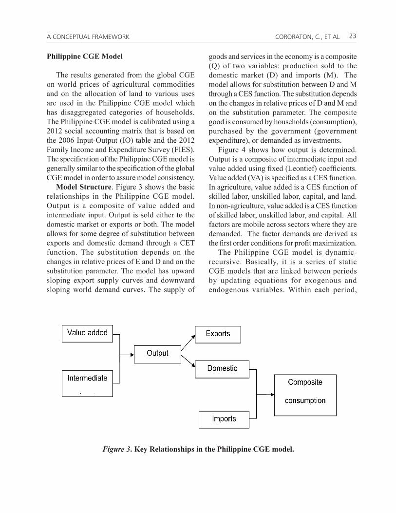
Model Structure. Figure 3 shows the basic relationships in the Philippine CGE model. Output is a composite of value added and intermediate input. Output is sold either to the domestic market or exports or both. The model allows for some degree of substitution between exports and domestic demand through a CET function. The substitution depends on the changes in relative prices of E and D and on the substitution parameter. The model has upward sloping export supply curves and downward sloping world demand curves. The supply of

goods and services in the economy is a composite (Q) of two variables: production sold to the domestic market (D) and imports (M). The model allows for substitution between D and M through a CES function. The substitution depends on the changes in relative prices of D and M and on the substitution parameter. The composite good is consumed by households (consumption), purchased by the government (government expenditure), or demanded as investments.

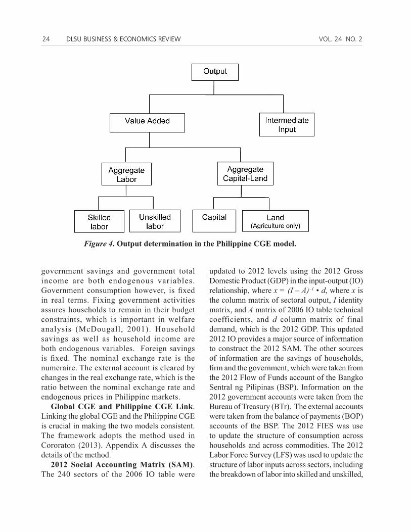
Figure 4 shows how output is determined. Output is a composite of intermediate input and value added using fixed (Leontief) coefficients. Value added (VA) is specified as a CES function. In agriculture, value added is a CES function of skilled labor, unskilled labor, capital, and land. In non-agriculture, value added is a CES function of skilled labor, unskilled labor, and capital. All factors are mobile across sectors where they are demanded. The factor demands are derived as the first order conditions for profit maximization.

The Philippine CGE model is dynamic-recursive. Basically, it is a series of static CGE models that are linked between periods by updating equations for exogenous and endogenous variables. Within each period,

Figure 3. Key Relationships in the Philippine CGE model.


government savings and government total income are both endogenous variables. Government consumption however, is fixed in real terms. Fixing government activities assures households to remain in their budget constraints, which is important in welfare analysis (McDougall, 2001). Household savings as well as household income are both endogenous variables. Foreign savings is fixed. The nominal exchange rate is the numeraire. The external account is cleared by changes in the real exchange rate, which is the ratio between the nominal exchange rate and endogenous prices in Philippine markets.

Global CGE and Philippine CGE Link. Linking the global CGE and the Philippine CGE is crucial in making the two models consistent. The framework adopts the method used in Cororaton (2013). Appendix A discusses the details of the method.

2012 Social Accounting Matrix (SAM). The 240 sectors of the 2006 IO table were

updated to 2012 levels using the 2012 Gross Domestic Product (GDP) in the input-output (IO) relationship, where x = (I – A)–1 • d, where x is the column matrix of sectoral output, I identity matrix, and A matrix of 2006 IO table technical coefficients, and d column matrix of final demand, which is the 2012 GDP. This updated 2012 IO provides a major source of information to construct the 2012 SAM. The other sources of information are the savings of households, firm and the government, which were taken from the 2012 Flow of Funds account of the Bangko Sentral ng Pilipinas (BSP). Information on the 2012 government accounts were taken from the Bureau of Treasury (BTr). The external accounts were taken from the balance of payments (BOP) accounts of the BSP. The 2012 FIES was use to update the structure of consumption across households and across commodities. The 2012 Labor Force Survey (LFS) was used to update the structure of labor inputs across sectors, including the breakdown of labor into skilled and unskilled,

Figure 4. Output determination in the Philippine CGE model.


where unskilled labor is defined as labor without high school diploma.

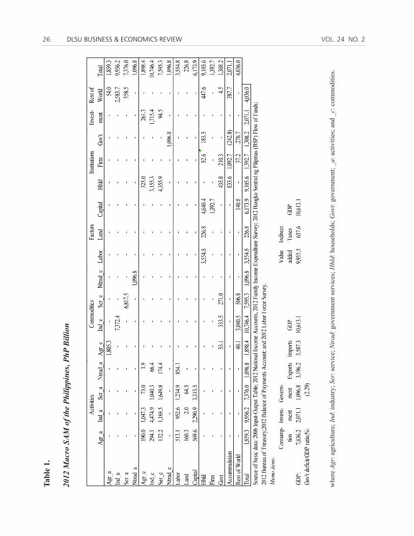
This set of information is combined using a SAM framework. Because data come from various sources, initially the resulting SAM is not balanced. Adjustments are needed to balance the SAM. There are several methods available in the literature to balance a SAM. In the present case, the SAM adjustments were made using an entropy method (Fofana, Lemelin, & Cockburn, 2005). The resulting macro SAM is shown in the table below.3 In 2012, GDP of the Philippine economy was PhP10,613.1 billion. The government-deficit-to-GDP was -2.29%. Table 1 shows the 2012 Macro Philippine SAM.

Philippine Poverty Micro simulation Model

The CGE results are used in a poverty microsimulation model to simulate the effects on poverty and income distribution. There are several approaches to linking CGE models with data in the household survey to analyze poverty and income distribution implications of changes in policies. One approach is a top-down method where the results of the CGE model with representative households are applied recursively to data in the household survey with no further feedback effects. In this method, the change in the income of the representative household in each of the household categories generated in the CGE model is used to estimate the change in the average income household of the same category (Decaluwé, Patry, Savard and Thorbecke, 2000). The form of the income distribution within each household category is assumed and the income variance within each category

is estimated using data in the household survey. The income variance does not change during the simulation.

Another approach is to integrate actual incomes in the household survey into the CGE model (Cockburn, 2001; Cororaton & Cockburn, 2007). Although this microsimulation approach poses no technical difficultly, it requires a computer with high computing power. This approach is better than the recursive approach because it allows for feedback effects from the economy to the households and vice versa. It also accounts for the heterogeneity of income sources and consumption patterns of households.

Another approach is to change the employment status of household head in the survey. Similar to Ganuza, Paes de Barros, and Vos (2002), the poverty microsimulation method used in the paper changes the employment status of household heads using information generated from the CGE model after a policy change. If the household head is unemployed initially in the household survey, he/she may gain employment if he/she is in the expanding sector of the economy after the policy shock.1 In contrast, if the household head is employed initially, he/she may become unemployed if he/she belongs to a contracting sector of the economy after the policy shock. This change in the employment status of household heads after the policy shock together with the change in wages from the CGE model affects labor income of households (Cororaton & Corong, 2009; Cororaton, 2013).

Changes in capital and land income derived from the Philippine CGE will be introduced in the poverty microsimulation as changes in other household income.


whe

re A

gr: a

gric

ultu

re; I

nd: i

ndus

try; S

er: s

ervi

ce; N

trad

: gov

ernm

ent s

ervi

ces;

Hhl

d: h

ouse

hold

s; G

ovt:

gove

rnm

ent;

_a: a

ctiv

ities

; and

_c:

com

mod

ities

.

Tabl

e 1.

2012

Mac

ro S

AM

of t

he P

hilip

pine

s, Ph

P B

illio

n


NOTES

1 However, the interactions between crops, pests and pathogens are complex and poorly understood in the context of climate change.

2 AEZ is a land resource mapping unit, defined in terms of climate, landform, and soils and has a specific range of potentials and constraints for cropping (FAO, 1996).

3 The table only shows the macro SAM. However, the updated 2012 SAM is very detailed in sectoral breakdown comprising of 240 sectors, skilled and unskilled labor, and 10 household groups (decile). The list of these sectors is available upon request from the authors.

REFERENCES

Asian Development Bank. (2011). Climate change and food security in the Pacific. Rethinking the options. Mandaluyong City, Philippines: Asian Development Bank.

Butt, T. A., McCarl, B. A., Angerer, J., Dyke, P. T., & Stuth, J. W. (2005). The economic and food security implications of climate change in Mali. Climatic Change, 68(3), 355-378.

Cockburn, J., (2001). Trade liberalization and poverty in Nepal: A computable general equilibrium micro simulation analysis [mimeo]. Department of Economics, Laval University, Québec, Canada.

Cororaton, C. B. (2013). Economic impact analysis of the reduction in sugar tariffs under the ASEAN trade in goods agreement: The case of the Philippine sugar sector (GII Working Paper No. 2013-1). Virginia, USA: Virginia Tech.

Cororaton, C. B., & Orden, D. (2014). Analyzing the potential economic effects of Philippine participation in the Trans-Pacific Partnership (TPP) agreement. Virginia, USA: Virginia Tech.

Cororaton, C. B., & Cockburn, J. (2007). Trade reform and poverty—Lessons from the Philippines: A CGE-microsimulation analysis. Journal of Policy Modeling, 29(1), 141-163.

Cororaton, C. B., & Corong, E. L. (2009). Philippine agricultural and food policies: Implications for poverty and income distribution (International Food Policy Research Institute Report No. 161). Washington, DC: IFPRI.

Cororaton C. B., Clarete, R., & Sharma, M. (2013) “Impact of Alternative Philippine Rice Policies on Poverty and Income Distribution”. A paper submitted to the World Bank.

Decaluwé, B., A. Patry, L. Savard et E. Thorbecke (2000), “Poverty Analysis within a General Equilibrium Framework”, Working paper 9909, Department of Economics, Laval University.

De Hoyos, R. (2008). Global income distribution dynamics (GIDD) Washington, DC: World Bank.

Estrades, C. (2013). Guide to microsimulations linked to CGE models: How to introduce analysis of poverty and income distribution in CGE-based studies (African Growth & Development Policy or AGRODEP Technical Note TN-09). Washington, DC: IFPRI.

Fofana, I., Lemelin, A., & Cockburn, J. (2005). Balancing a social accounting matrix: Theory and application [Training material]. Centre Interuniversitairesur le Risque, les PolitiquesEconomiques et l’Emploi, Universite Laval, Quebec. Retrieved from http://www.pep-net.org/fileadmin/medias/pdf/sambal.pdf

Food and Agriculture Organization (FAO). (1996). Agro-ecological zoning guidelines, FAO Soils Bulletin 73. Place published: FAO Land and Water Division. See more at: http://www.fao.org/nr/gaez/publications/en/#sthash.fS3FMiTz.dpuf

Ganuza, E., Paes de Barros, R., & Vos, R. (2002). Labor market adjustment, poverty and inequality during liberalisation. In: R. Vos, L. Taylor, & R. Paes de Barros (Eds.), Economic liberalisation, distribution and poverty: Latin America in the 1990s (pp. 54-88). Cheltenham (UK) and Northampton (US): Edward Elgar Publishers.


Golub, A., Hertel, T. W., & Sohngen, B. (2009). 10 Land use modelling in a recursively dynamic GTAP framework. Economic Analysis of Land Use in Global Climate Change Policy, 235-278.

Gornall, J. et al. (2010). Implications of climate change for agricultural productivity in the early 21st century. Phil. Trans. R. Soc. B, 365 ( ), 2973–2989.

Gregorio, A.D. (2005). Land Cover Classification System: Classification concepts and user manual, Software version (2). Rome: Food and Agriculture Organization of the United Nations.

Hertel, T. and L. A. Winters (2006). Poverty and the Doha: Impacts of the Doha Development Agenda.New York: Palgrave Macmillan, and Washington, D.C.: The World Bank.

Horridge, M. and Z. Fan (2006). Shocking a Single-Country CGE Model with Export Prices and Quantities from a Global Model. In Poverty and the WTO: Impacts of the Doha Development Agenda. (Thomas Hertel and L. Alan Winters, eds). New York: Palgrave Macmillan, and Washington, D.C.: The World Bank. pp. 94-104.

Intergovernmental Panel on Climate Change (IPCC). (2007). Fourth assessment report of the Intergovernmental Panel on Climate Change . Cambridge, UK: Cambridge University Press.

Lin, B. B., Chappell, M. J., Vandermeer, J., Smith, G., Quintero, E., Bezner-Kerr, R., ... & Perfecto14, I. (2012). Effects of industrial agriculture on climate change and the mitigation potential of small-scale agro-ecological farms. Animal Science Reviews 2011, 69-86.

Zhai, F., Lin, T. & Byambadorj, E. (2009). A general equilibrium analysis of the impact of climate change on agriculture in the People’s Republic of China. Asian Development Review, 26(1), 206-225.

Lobell, D. B., Burke, M. B., Tebaldi, C., Mastrandrea, M. D., Falcon, W. P., & Naylor, R. L. (2008). Prioritizing climate change adaptation needs for food security in 2030. Science, 319(5863), 607-610.

McDougall, R. (2001). A new regional household demand system for GTAP (GTAP Technical Paper No.20). West Lafayette, Indiana, U.S.A.: Global Trade Analysis Project, Purdue University.

Moss R.H., Edmonds, J.A., Hibbard, K.A., Manning, M.R., Rose, S.K., van Vuuren, D.P., Carter, T.R., Emori, S., Kainuma, M., Kram, T., Meehl, G.A., Mitchell, J.F., Nakicenovic, N., Riahi, K., Smith, S.J., Stouffer, R.J., Thomson, A.M., Weyant, J.P., Wilbanks, T.J. (2010). The next generation of scenarios for climate change research and assessment. Nature, 463, 747-756.

National Statistical Coordinating Board (NSCB) (2010). NSCB Resolution No.7 Series of 2010 –Approving and Adopting the Official Concepts and Definitions for Statistical Purposes for the Environment and Natural Resources Sector, Batch 2, Land/Soil Resources Subsector. Makati City: NSCB.

Nelson, G.C., Rosegrant, M. W., Koo, J., Robertson, R., Sulser, T., Zhu, T., Ringler, C., Msangi, S., Palazzo, A., Batka, M., Magalhaes, M., Valmonte-Santos, R., Ewing, M., Lee, D. (2009). Impact on Agriculture and Costs of Adaptation. Food Policy Report No. 21. Washington, D.C.: International Food Policy Research Institute.

Palatnik, R.R., & Roson, R. (2009). Climate change assessment and agriculture in general equilibrium models: Alternative modeling strategies (Nota di Lavoro 67). Working Paper No. 08/WP/2009, Department of Economics. Venice: University of Ca’ Foscari .

Ronneberger, K., Berrittella, M., Bosello, F., Tol, R. (2009). Klum@Gtap: Introducing biophysical aspects of land-use decisions into a computable general equilibrium model


a coupling experiment. Environmental Modeling Assessment, 14(2), 149-169.

Timilsina, G.R., van der Mensbruggle, D., Mevel, S., &Beghin, J.C. (2012) “The Impacts of Biofuel Targets on Land-Use Change and Food Supply: A Global CGE Assessment.” Agricultural Economics, 43(3), 35-332.

Turner II, B. L., Lambin, E. F., & Reenberg, A. (2007). The emergence of land change science for global environmental change and sustainability. Proceedings of the National Academy of Sciences (PNAS), 104(52), 20666–20671.

van der Mensbrugghe, D. (2008). The environmental impact and sustainability applied general equilibrium (ENVISAGE) model. Washington, DC: The World Bank.

Vermeulen, S.J., Aggarwal, P.K., Ainslie, A., Angelone, C., Campbell, B.M., Challinor, A.J., Hansen, J, Ingram, J.S.I., Jarvis, A., Kristjanson, P., Lau, C., Thornton, P.K., Wollenberg E. (2010). Agriculture, food security and climate change: Outlook for

knowledge, tools and action (CCAFS Report No. 3). Copenhagen: CGIAR-ESSP Program on Climate Change, Agriculture and Food Security.

Wang, Zhang, You, and Pal. (2011). “Collaborative Research: A Pilot Project on Interactive Climate and Land Use Predictions.” NSF AGS, University of Connecticut, International Food Policy Research Institute, Loyola Marymount University. LOI 02170299: Wang, Zhang, You. Pal (Principal Investigators). Manuscript.

Wang, Y., Kockelman, K.M., & Wang, X. (2011). Anticipation of land use change through use of geographically weighted regression models for discrete response. Transportation Research Record, 2245, 111–123.

Zhai, F., & Zhuang, J. (2009). Agricultural impact of climate change: A general equilibrium analysis with special reference to Southeast Asia (ADBI Working Paper No. 131). Tokyo, Japan: Asian Development Bank Institute.


APPENDIX A. LINKING GLOBAL ANDTHE PHILIPPINE MODELS

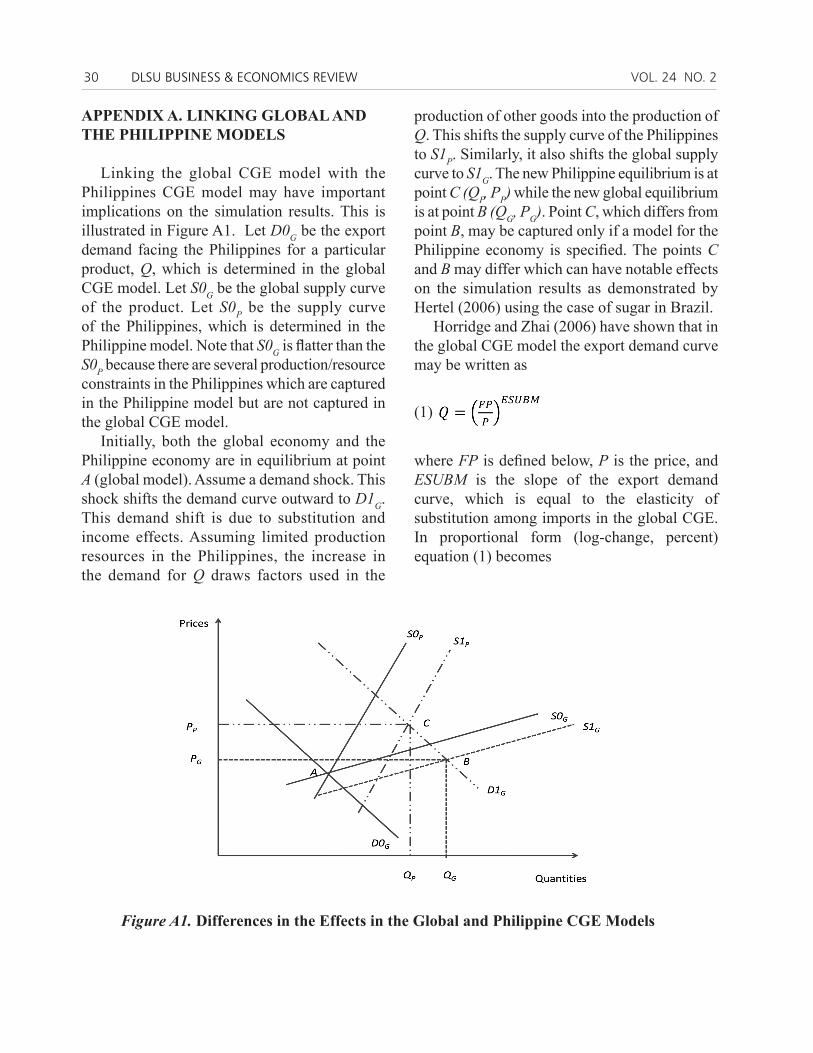
Linking the global CGE model with the Philippines CGE model may have important implications on the simulation results. This is illustrated in Figure A1. Let D0G be the export demand facing the Philippines for a particular product, Q, which is determined in the global CGE model. Let S0G be the global supply curve of the product. Let S0P be the supply curve of the Philippines, which is determined in the Philippine model. Note that S0G is flatter than the S0P because there are several production/resource constraints in the Philippines which are captured in the Philippine model but are not captured in the global CGE model.

Initially, both the global economy and the Philippine economy are in equilibrium at point A (global model). Assume a demand shock. This shock shifts the demand curve outward to D1G. This demand shift is due to substitution and income effects. Assuming limited production resources in the Philippines, the increase in the demand for Q draws factors used in the

production of other goods into the production of Q. This shifts the supply curve of the Philippines to S1P. Similarly, it also shifts the global supply curve to S1G. The new Philippine equilibrium is at point C (QP, PP) while the new global equilibrium is at point B (QG, PG). Point C, which differs from point B, may be captured only if a model for the Philippine economy is specified. The points C and B may differ which can have notable effects on the simulation results as demonstrated by Hertel (2006) using the case of sugar in Brazil.

Horridge and Zhai (2006) have shown that in the global CGE model the export demand curve may be written as

(1)

where FP is defined below, P is the price, and ESUBM is the slope of the export demand curve, which is equal to the elasticity of substitution among imports in the global CGE. In proportional form (log-change, percent) equation (1) becomes

Figure A1. Differences in the Effects in the Global and Philippine CGE Models


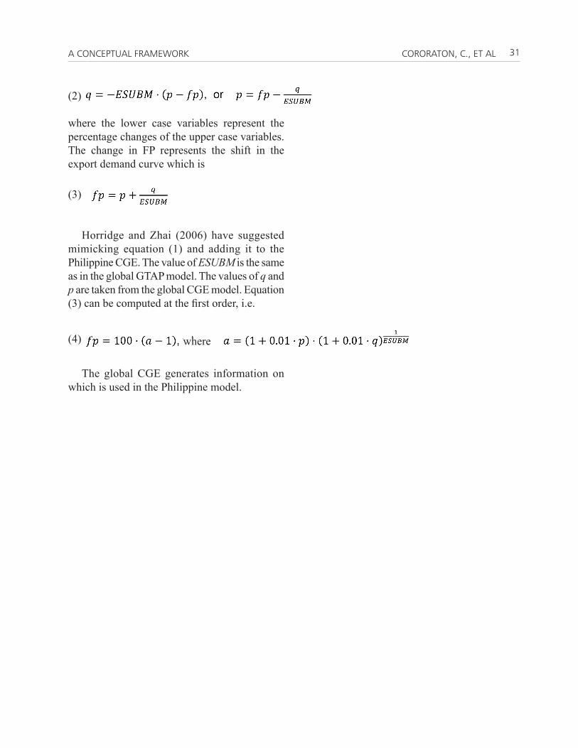
(2)

where the lower case variables represent the percentage changes of the upper case variables. The change in FP represents the shift in the export demand curve which is

(3)

Horridge and Zhai (2006) have suggested mimicking equation (1) and adding it to the Philippine CGE. The value of ESUBM is the same as in the global GTAP model. The values of q and p are taken from the global CGE model. Equation (3) can be computed at the first order, i.e.

(4)

The global CGE generates information on which is used in the Philippine model.

where

A Conceptual Framework for Estimating the Impact of Climatic Uncertainty and Shocks on Land Use,...

Documents

Transcript of A Conceptual Framework for Estimating the Impact of Climatic Uncertainty and Shocks on Land Use,...