Calculations for 3500 3Flex - Micromeritics

CALCULATIONSSep 2016(Ver 4.x)

3FLEX™

SURFACE CHARACTERIZATION ANALYZER

Table of Contents

Alpha-S Method 1

BET Surface Area 2

BET Surface Area for TCD 3

BJH Pore Volume and Area Distribution 5

Crystallite Size for Chemical Adsorption 14

DFT (Density Functional Theory) 15

Dollimore-Heal Adsorption 18

Dubinin-Astakhov 20

Dubinin-Radushkevich 24

Equation of State 26

Equilibration 27

f-Ratio Method 28

First Order Kinetics for TCD 29

Free Space for Chemical Adsorption 30

Freundlich Isotherm 31

Horvath-Kawazoe 32

Injection Loop Calibration for TCD 42

Calculations for the 3500 3Flex(Ver 4.x) — Sep 2016 i

Langmuir Surface Area for Chemical Adsorption 43

Langmuir Surface Area for Physical Adsorption 44

Langmuir Surface Area for TCD 46

Metal Dispersion for Chemical Adsorption 48

Metallic Surface Area for Chemical Adsorption 49

Metallic Surface Area for TCD 50

MP-Method 51

Particle Size for TCD 53

Peak Area Quantity for TCD 54

Percent Dispersion for TCD 55

Quantity Adsorbed for Chemical Adsorption 56

Quantity Adsorbed for Physical Adsorption 57

Quantity Adsorbed for TCD 60

Quantity of Gas for TCD 61

Real Gas Equation of State for Chemical Adsorption 62

Relative Pressure 63

Saturation Pressure 64

SPC Report Variables 65

Calculations for the 3500 3Flex(Ver 4.x) — Sep 2016 ii

Summary Report 67

t-Plot 69

Temkin Isotherm 70

Thermal Transpiration Correction 71

Thickness Curve 72

Weighted Metal Parameters 74

Calculations for the 3500 3Flex(Ver 4.x) — Sep 2016 iii

ALPHA-S METHOD

The alpha-S curve is calculated from the reference isotherm by dividing each quantity adsorbed bythe quantity adsorbed at 0.4 relative pressure.

α =Q

Qii

0.4

whereQ0.4 is found by linear interpolation.

A least-squares analysis fit is performed on the (αi,Qads,i) data pairs where αi is the independentvariable andQads,i is the dependent variable. The following are calculated:

a. Slope (S cm3/g STP)b. Y-intercept (Q0 cm

3/g STP)c. Error of the slope (cm3/g STP)d. Error of the Y-intercept (cm3/g STP)e. Correlation coefficient

Surface area is calculated as:

A =A S

Q

ref

0.4

Pore size is calculated as:

Q V

22414cm STP

mol

3

0

where Vmol is liquid molar volume from the fluid property information.

Alpha-S Method

Calculations for the 3500 3Flex(Ver 4.x) — Sep 2016 1

BET SURFACE AREAThe BET1 ) transformation is calculated as:

( )y =

1

Q ρ / ρ − 10

A least-squares fit is performed on the (Prel, y). The following are calculated:

a. Slope (S cm3/g STP)b. Y-intercept (y0 cm

3/g STP)c. Uncertainty of the slope (u(s) cm3/g STP)d. Uncertainty of the Y-intercept (u(y0) cm

3/g STP)e. Correlation coefficient

Using the results of the above calculations, the following can be calculated:

BET Surface Area (m2/g):

( )A = × 10 m / nm

A N

V s + y

−18 2 2s

0

m A

m

BET C value:

C = + 1s

y0

Quantity in the Monolayer (cm3/g STP):

Q = =m

1

Cy

1

s + y0 0

Error of the BET Surface Area (m2/g):

( ) ( )u(A ) =s

u s + u y

s + y

2 20

0

1 ) Brunauer, S.; Emmett, P.H.; and Teller, E., J. Am. Chem. Soc. 60, 309 (1938).

BET Surface Area


BET Surface Area for TCD

BET SURFACE AREA FOR TCDSurface area is calculated as the number of molecules in themonolayer times the area of amolecule. The result is divided by samplemass to give the specific surface area.

A = Q N A / mBET m,mol, A α

The quantity of adsorbate in themonolayer is determined by fitting BET-transformed data frommultiple experiments.

( )B =i

P

Q 1 − P

rel,i

i rel,i

P = crel,i i

P

P

α

0

The slope s and offset y0 of the best-fit line throughBi vs. Prel,i are found.

Q =m

1

s + y0

C = s / y − 10

Uncertainty in the surface area is estimated from the uncertainty in the fit parameters.

( ) (

u(A ) = ABET BET

u s + u y

s + y

2 20

0

where

ABET = specific BET surface areaQm,mol = quantity of adsorbate in themonolayer in molesNA = Avogadro constant: 6.02214129 × 1023mol-1

Aα = adsorbate cross-sectional aream = samplemassBi = BET transform of the data from experiment iQi = cumulative quantity adsorbed for all peaks in experiment $iPrel,i = relative pressure for experiment iPα = entered ambient pressureP0 = entered saturation pressure for the active gasci = active gas concentration in experiment iC = BET C values = slope of best-fit line

3 Calculations for the 3500 3Flex(Ver 4.x) — Sep 2016

y0 = intercept of best-fit lineu(x) = uncertainty of x

SINGLE-POINTFor single experiment themonolayer quantity calculation becomes

s = B / Prel

y = 00

( )Q = Q 1 − Pm rel

BET Surface Area for TCD


BJH PORE VOLUME AND AREA DISTRIBUTIONFor adsorption data, the relative pressure and quantity adsorbed data point pairs collected during ananalysismust be arranged in reverse order fromwhich the points were collected during analysis. Allcalculations are performed based on a desorptionmodel, regardless of whether adsorption ordesorption data are being used.

The data used in these calculationsmust be in order of strictly decreasing numerical value. Pointswhich do not meet this criterion are omitted. The remaining data set is composed of relative pressure(P), quantity adsorbed (Q) pairs from (P1,Q1) to (P,Qn) where (Pn = 0,Qn = 0) is assumed as a finalpoint. Each data pair represents an interval boundary (or desorption step boundary) for intervals i=1to i=n-1where n = total number of (P,Q) pairs.

Generally, the desorption branch of an isotherm is used to relate the amount of adsorbate lost in adesorption step to the average size of pores emptied in the step. A pore loses its condensed liquidadsorbate, known as the core of the pore, at a particular relative pressure related to the core radiusby the Kelvin1 ) equation. After the core has evaporated, a layer of adsorbate remains on the wall ofthe pore. The thickness of this layer is calculated for a particular relative pressure from the thicknessequation. This layer becomes thinner with successive decreases in pressure, so that themeasuredquantity of gas desorbed in a step is composed of a quantity equivalent to the liquid cores evaporatedin that step plus the quantity desorbed from the pore walls of poreswhose cores have beenevaporated in that and previous steps. Barrett, Joyner, and Halenda2 ) developed themethod(known as the BJH method) which incorporates these ideas. The algorithm used is animplementation of the BJH method.

EXPLANATION OF TERMSA pore filled with condensed liquid nitrogen has three zones:

l Core. The core - evaporates all at once when the critical pressure for that radius is reached; therelationship between the core radius and the critical pressure is defined by the Kelvin equation.

l Adsorbed layer. The adsorbed layer - composed of adsorbed gas that is stripped off a bit at atime with each pressure step; the relationship between the thickness of the layer and the relativepressure is defined by the thickness equation.

l Walls of the cylindrical pore. Thewalls of the cylindrical pore - the diameter of the empty poreis required to determine the pore volume and pore area. End area is neglected.

1 ) Kelvin, J. (published under the name of Sir William Thomson),Phil. Mag. 42, 448-452 (1871).2 ) Barrett, E.P.; Joyner, L.S.; and Halenda, P.P., J. Am. Chem. Soc. 73, 373-380 (1951).

BJH Pore Volume and Area Distribution


CALCULATIONSThe quantities adsorbed (Qa) are converted to the liquid equivalent volumes (Vl, cm3/g):

Vl =iQ V

22414cm STP

i mol

3

whereVmol is the liquid molar volume from the fluid property information.

The relative pressure (Pi) is assumed to be close to unity so that substantially all the pores in thesample are filled.

The corresponding Kelvin core radius is calculated. Only pores smaller than this size will be included:

( ) ( )Rc =i

−A

1 + F ln Pi

where

A = adsorbate property factor (from theBJH Adsorptive Optionswindow)F = fraction of pores open at both ends (from theBJH Adsorption Report Optionswin-

dow or theBJH Desorption Report Options window); assumed to be zero fordesorption

Rc = Kelvin radius (Å) of core

This radius will be adjusted for the thickness of the adsorbed layer during subsequent calculationsteps.



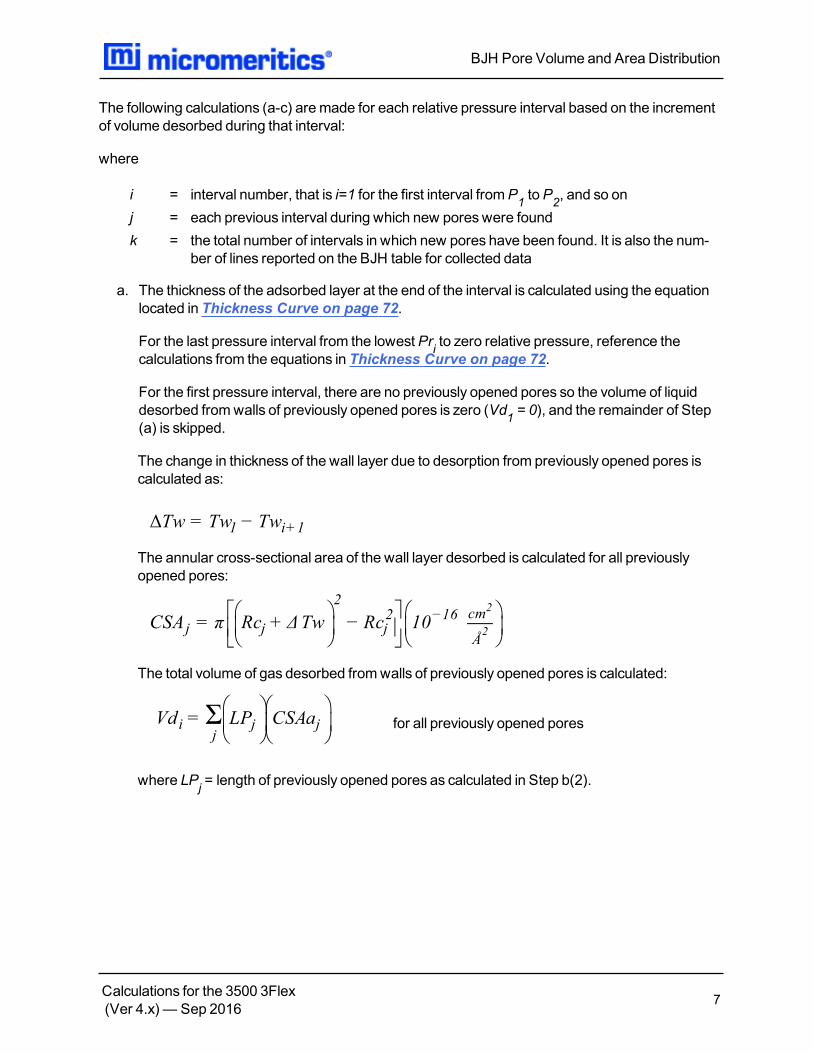
The following calculations (a-c) aremade for each relative pressure interval based on the incrementof volume desorbed during that interval:

where

i = interval number, that is i=1 for the first interval fromP1 toP2, and so onj = each previous interval during which new poreswere foundk = the total number of intervals in which new pores have been found. It is also the num-

ber of lines reported on the BJH table for collected data

a. The thickness of the adsorbed layer at the end of the interval is calculated using the equationlocated in Thickness Curve on page 72.

For the last pressure interval from the lowestPri to zero relative pressure, reference thecalculations from the equations in Thickness Curve on page 72.

For the first pressure interval, there are no previously opened pores so the volume of liquiddesorbed fromwalls of previously opened pores is zero (Vd1 = 0), and the remainder of Step(a) is skipped.

The change in thickness of the wall layer due to desorption from previously opened pores iscalculated as:

Tw = Tw − Tw∆ 1 i+1

The annular cross-sectional area of the wall layer desorbed is calculated for all previouslyopened pores:

CSA = π Rc + ∆Tw − Rc 10j j

2

j2 −16 cm

Å

2

2

The total volume of gas desorbed fromwalls of previously opened pores is calculated:

ΣVd = LP CSAai

jj j for all previously opened pores

where LPj = length of previously opened pores as calculated in Step b(2).



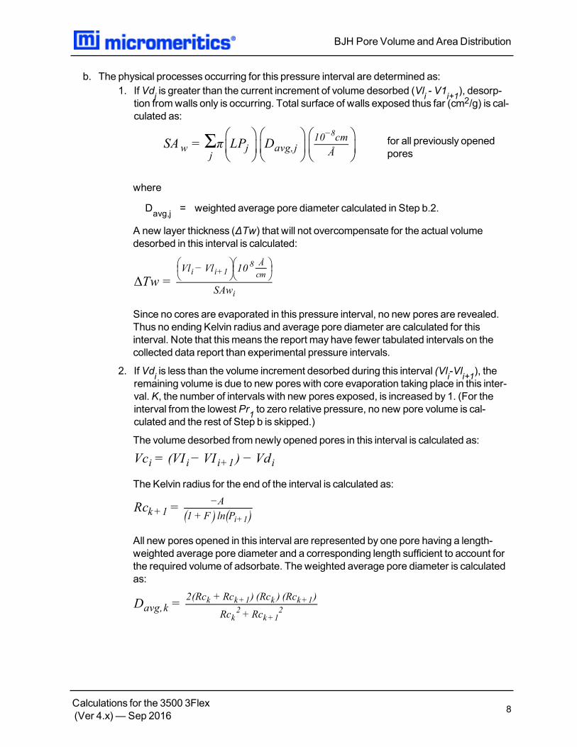
b. The physical processes occurring for this pressure interval are determined as:1. If Vdj is greater than the current increment of volume desorbed (Vli - V1i+1), desorp-

tion fromwalls only is occurring. Total surface of walls exposed thus far (cm2/g) is cal-culated as:

ΣSA = π LP Dw

jj avg,j

10 cm

Å

−8for all previously openedpores

where

Davg,j = weighted average pore diameter calculated in Step b.2.

A new layer thickness (ΔTw) that will not overcompensate for the actual volumedesorbed in this interval is calculated:

Tw =∆

Vl − Vl 10

SAw

i i+18 Å

cm

i

Since no cores are evaporated in this pressure interval, no new pores are revealed.Thus no ending Kelvin radius and average pore diameter are calculated for thisinterval. Note that thismeans the report may have fewer tabulated intervals on thecollected data report than experimental pressure intervals.

2. If Vdi is less than the volume increment desorbed during this interval (Vli-Vli+1), theremaining volume is due to new poreswith core evaporation taking place in this inter-val. K, the number of intervals with new pores exposed, is increased by 1. (For theinterval from the lowestPr1 to zero relative pressure, no new pore volume is cal-culated and the rest of Step b is skipped.)

The volume desorbed from newly opened pores in this interval is calculated as:

Vc = (VI − VI ) − Vdi i i+1 i

The Kelvin radius for the end of the interval is calculated as:

( ) ( )Rc =k+1

−A

1 + F ln Pi+1

All new pores opened in this interval are represented by one pore having a length-weighted average pore diameter and a corresponding length sufficient to account forthe required volume of adsorbate. The weighted average pore diameter is calculatedas:

D =avg,k2(Rc + Rc ) (Rc ) (Rc )

Rc + Rc

k k+1 k k+1

k2

k+12



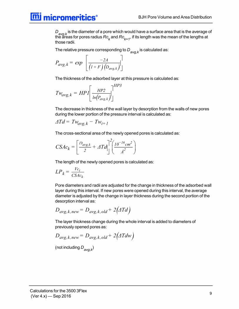
Davg,k is the diameter of a pore which would have a surface area that is the average ofthe areas for pores radiusRck andRck+1, if its length was themean of the lengths atthose radii.

The relative pressure corresponding toDavg,k is calculated as:

( ) ( )

P = expavg,k−2A

1 + F Davg,k

The thickness of the adsorbed layer at this pressure is calculated as:

( )

Tw = HP1avg,kHP2

ln P

HP3

avg,k

The decrease in thickness of the wall layer by desorption from the walls of new poresduring the lower portion of the pressure interval is calculated as:

∆Td = Tw − Twavg,k i+1

The cross-sectional area of the newly opened pores is calculated as:

CSAc = + ∆Tdk 2

210 cm

Å

avg,k−16 2

2

The length of the newly opened pores is calculated as:

LP =kVc

CSAc

i

k

Pore diameters and radii are adjusted for the change in thickness of the adsorbed walllayer during this interval. If new poreswere opened during this interval, the averagediameter is adjusted by the change in layer thickness during the second portion of thedesorption interval as:

( )D = D + 2 ∆Tdavg,k,new avg,k,old

The layer thickness change during the whole interval is added to diameters ofpreviously opened pores as:

( )D = D + 2 ∆Tdwavg,k,new avg,k,old

(not includingDavg,k)



The layer thickness change desorbed during this interval also is added to the radiicorresponding to the ends of the pressure intervals as:

Rc = Rc + ∆Twj,new j,old

for all exceptRck+1.

Steps a to c are repeated for each pressure interval.

After the above calculations have been performed, the diameters corresponding to theends of the intervals are calculated as:

( )Dp = 2 Rcj j

for allRcj includingRck+1.

The remaining calculations are based onDpi, Davg,i, and LPi. These calculations areonly done for Davg,i values that fall between theMinimumBJH diameter and theMaximumBJH diameter specified by the operator on theBJH Adsorption ReportOptionswindow or theBJH Desorption Report Optionswindow.

(1) Incremental Pore Volume (Vpi, cm3/g):

Vp = π L

i i

D

2

210 cm

Å

avg,i16 2

2

(2) Cumulative Pore Volume (Vpcum,i, cm3/g):

ΣVP = Vp for J ≤ 1cum,i

jj

(3) Incremental Surface Area (SAi, m2/g):

SA = π LP Di i

10 m

cm avg,i10 m

Å

−2 −10

(4) Cumulative Surface Area (SAcum,i, m2/g):

SA = ∑ SA J ≤ 1forcum,10 j

(5) dV/dD pore volume (dV/dDi, cm3/g-A):

=dV

dD

VP

Dp −Dpi

i

i i+1



(6) dV/dlog(D) pore volume (dV/dlog(D)i, cm3g):

=dDv

dlogD

VP

logi

i

Dpi

Dpi+1

(7) dA/dD pore area (dA/dDi, m2/g-A):

=dA

dD

SA

Dp −Dpi

i

i i+1

(8) dA/dlog(D) pore area [dA/dlog(D)i, m2/g]:

=dA

dlogD

SA

logi

i

Dpi

Dpi+1

For fixed pore size tables (if selected), the following calculations are performed

(1) Average Fixed Pore Size (DFavg,j, A):

DF =avg,j

DP +Dp

2

F j F j+1

calculated for all intervals in the fixed pore size table.

For the intervals with between theMinimumBJH diameter and theMaximumBJH diameter.

(2) Cumulative Pore volume (VpFcum,i, cm3/g):

( )VpF DpFcum,i = INTERP i+1

where INTERP(x) is the value interpolated from the functionX = Dpj+i and

Y = VPcum,i, using an AKIMA semi-spline interpolation.

(3) Incremental Pore Volume (VpFi, cm3/g):

VpF = VpF − VpFi cum,i cum,i−1

whereVpFcum,0 = 0.

(4) Cumulative Surface Area (SAFcum,i, m2/g):

( )SAFcum,i = INTERP DpFi+1

where INTERP(x) is the value interpolated from the functionX = Dpj+i and

Y = SAcum,j.



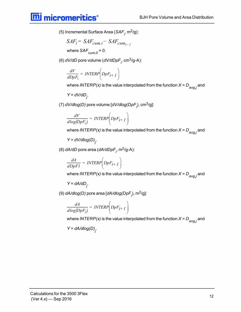
(5) Incremental Surface Area (SAFi, m2/g):

SAF = SAF − SAFi cum,i cumi−1

whereSAFcum,0 = 0.

(6) dV/dD pore volume (dV/dDpFi, cm3/g-A):

dV

dDpF= INTERP DpFi+1

i

where INTERP(x) is the value interpolated from the functionX = Davg,j and

Y = dV/dDj.

(7) dV/dlog(D) pore volume [dV/dlog(DpFi), cm3/g]:

( )

dV

dlog DpF= INTERP DpFi+1

i


Y = dV/dlog(D)j.

(8) dA/dD pore area (dA/dDpFi, m2/g-A):

dA

dDpF1= INTERP DpFi+1


Y = dA/dDj.

(9) dA/dlog(D) pore area [dA/dlog(DpFi), m2/g]:

( )

dA

dlog DpF= INTERP DpFi+1

i


Y = dA/dlog(D)j.



COMPENDIUM OF VARIABLES

ΔTd = thickness of layer desorbed fromwalls of newly opened pores (Å)ΔTw = thickness of adsorbed layer desorbed during interval (Å)A = adsorbate property factor; from theBJH Adsorptive OptionswindowCSA = analysis gasmolecular cross-sectional area (nm2), user-entered on theAdsorpt-

ive PropertieswindowCSAa = annular cross-sectional area of the desorbed layer (cm2)CSAc = cross-sectional area of opening of newly opened pores (cm2)Davg = average pore diameter (Å)Dp = pore (or core) diameter (Å)F = fraction of pores open at both ends; from theBJH Adsorption Report Optionswin-

dow or theBJH Desorption Report OptionswindowLP = length of pore (cm/g)P = relative pressureQ = quantity adsorbed expressed as a volume (cm3/g STP)Rc = Kelvin radius (Å) of coreSAw = total surface area of walls exposed (cm2/g)Tw = thickness of remaining adsorbed wall (Å)Vc = volume desorbed from cores of newly opened pores (cm3/g)Vd = volume of gas desorbed fromwalls of previously opened pores (cm3/g)Vl = liquid equivalent volume of volume adsorbed (cm3/g)Vmol = liquidmolar volume, from the fluid property information



CRYSTALLITE SIZE FOR CHEMICAL ADSORPTION

d =xtal1000k

ρAmetal

Where

k = shape factor; 6 for sphere, 5 for cubeρ = weighted average density of the activemetals

Crystallite Size for Chemical Adsorption


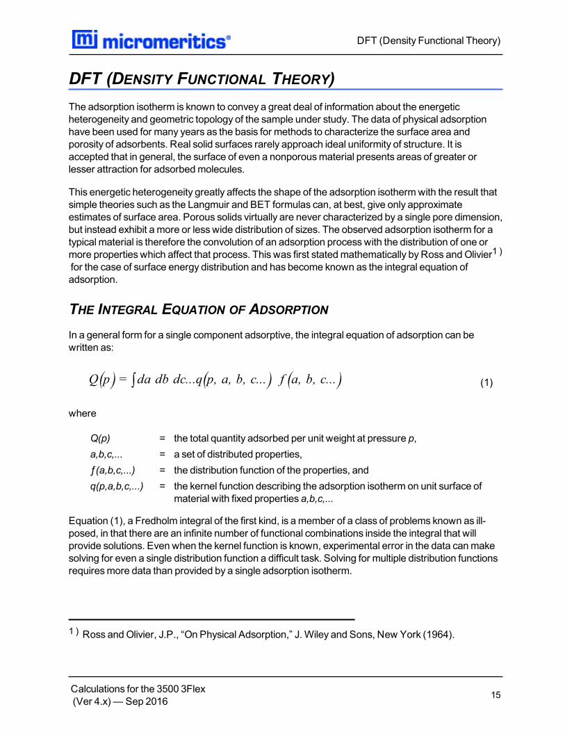
DFT (DENSITY FUNCTIONAL THEORY)The adsorption isotherm is known to convey a great deal of information about the energeticheterogeneity and geometric topology of the sample under study. The data of physical adsorptionhave been used for many years as the basis for methods to characterize the surface area andporosity of adsorbents. Real solid surfaces rarely approach ideal uniformity of structure. It isaccepted that in general, the surface of even a nonporousmaterial presents areas of greater orlesser attraction for adsorbedmolecules.

This energetic heterogeneity greatly affects the shape of the adsorption isothermwith the result thatsimple theories such as the Langmuir and BET formulas can, at best, give only approximateestimates of surface area. Porous solids virtually are never characterized by a single pore dimension,but instead exhibit a more or less wide distribution of sizes. The observed adsorption isotherm for atypical material is therefore the convolution of an adsorption processwith the distribution of one ormore properties which affect that process. This was first statedmathematically by Ross andOlivier1 )for the case of surface energy distribution and has become known as the integral equation ofadsorption.

THE INTEGRAL EQUATION OF ADSORPTIONIn a general form for a single component adsorptive, the integral equation of adsorption can bewritten as:

( ) ( ) ( )∫Q p = da db dc...q p, a, b, c... f a, b, c... (1)

where

Q(p) = the total quantity adsorbed per unit weight at pressure p,a,b,c,... = a set of distributed properties,ƒ(a,b,c,...) = the distribution function of the properties, andq(p,a,b,c,...) = the kernel function describing the adsorption isotherm on unit surface of

material with fixed properties a,b,c,...

Equation (1), a Fredholm integral of the first kind, is amember of a class of problems known as ill-posed, in that there are an infinite number of functional combinations inside the integral that willprovide solutions. Even when the kernel function is known, experimental error in the data canmakesolving for even a single distribution function a difficult task. Solving for multiple distribution functionsrequiresmore data than provided by a single adsorption isotherm.

1 ) Ross andOlivier, J.P., “On Physical Adsorption,” J. Wiley and Sons, New York (1964).

DFT (Density Functional Theory)


APPLICATION TO SURFACE ENERGY DISTRIBUTIONUnder certain conditions, an energetically heterogeneous surfacemay be characterized by adistribution of adsorptive energies. The conditions are that the sample is not microporous, i.e., thatadsorption is taking place on essentially a free surface with no pore filling processes at least to about0.2 relative pressure. Secondly, that each energetically distinct patch contributes independently tothe total adsorption isotherm in proportion to the fraction of the total surface that it represents. Thiscondition is satisfied if the patches are relatively large compared to an adsorptivemolecule, or if theenergy gradient along the surface is not steep. In mathematical terms, this concept is expressed bythe integral equation of adsorption in the following form:

( ) ( ) ( )∫Q p = dϵ q p, ϵ f ϵ (2)

where

Q(p) = the experimental quantity adsorbed per gram at pressure p,q(p,ε) = the quantity adsorbed per unit area at the same pressure, p, on an ideal free sur-

face of energy ε, andƒ(ε) = the total area of surface of energy ε in the sample.

The exact form of the energy-dependent term depends on the form of themodel isothermsexpressed in the kernel function and is provided in themodel description.

APPLICATION TO PORE SIZE DISTRIBUTIONSimilarly, a sample of porousmaterial may be characterized by its distribution of pore sizes. It isassumed in this case that each pore acts independently. Each pore size present then contributes tothe total adsorption isotherm in proportion to the fraction of the total area of the sample that itrepresents. Mathematically, this relation is expressed by:

( ) ( ) ( )∫Q p = dH q p, H f H (3)

where

Q(p) = the experimental quantity adsorbed at pressure p,q(p,H) = the quantity adsorbed per unit area at the same pressure, p, in an ideal pore of

sizeH, andƒ(H) = the total area of pores of sizeH in the sample.



Numerical values for the kernel functions in the form of model isotherms can be derived frommodernstatistical mechanics such as density functional theory or molecular simulations, or can be calculatedfrom one of various classical theories based on the Kelvin equation. Several types are found in themodels library.

PERFORMING THE DECONVOLUTIONThe integrations in equations (2) and (3) are carried out over all surface energies or pore sizes in themodel. The functions q(p,ε) and q(p,H), which we call the kernel functions, are contained in numericform asmodel isotherms. Because, in general, there is no analytic solution for equation (1), theproblem is best solved in a discrete form; the integral equation for any distributed property Zbecomes a summation

ΣQ p = q p, Z f Zi

i i (4)

Given a set of model isotherms, q(p,Z), from amodel chosen from themodels library and anexperimental isotherm,Q(p), contained in a sample information file, the software determines the setof positive values f(Z) that most nearly, in a least squares sense, solves equation (4). The distributedproperty, surface energy or pore size, is then displayed on theReport Optionswindow as a selectionof tables or graphs.

REGULARIZATIONDFT allows a selectable regularization (also referred to as smoothing) constraint to be applied duringthe deconvolution process to avoid over-fitting in the case of noisy data or ill-fittingmodels. Themethod used is based on co-minimization of the second derivative of the distribution. The relativeweight given to this term is determined by the value of the regularization parameter, which is set ontheDFT Pore Size or Surface Energywindow and also is shown in the header of reports. The valueof the regularization parameter varies from zero (for no second derivative constraint) to ten(indicating a weight equal to minimizing the residuals), or even larger. When the distribution andresiduals obtained change little with the value of the regularization parameter, it indicates that thechosenmodel provides a good representation of the data. Conversely, a large sensitivity to theregularization parameter might indicate inadequate data or a poor choice of model to represent thedata.



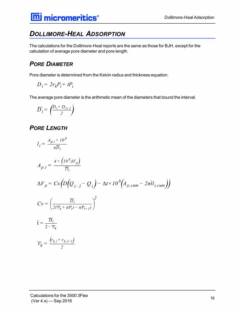
DOLLIMORE-HEAL ADSORPTIONThe calculations for the Dollimore-Heal reports are the same as those for BJH, except for thecalculation of average pore diameter and pore length.

PORE DIAMETERPore diameter is determined from the Kelvin radius and thickness equation:

D = 2r P + tPi k i i

The average pore diameter is the arithmeticmean of the diameters that bound the interval.

( )D =iD +D

2

i i+1

PORE LENGTH

l =iA + 10

πD

, i8

i

( )A =p,i

4 × 10 ∆V8

p

i

( ( ) ( ))V = Cυ D Q − Q − t×10 A − 2πtl∆ ∆i−1 i

8,c m i,c m

Cv =D

2( r + t(P ) − t(P )

2i

k i i+1

t =D

2− r

i

k

( )r =k

r + r

2

k,i k,i+1

Dollimore-Heal Adsorption


where

ΔVp = Change in pore volumeAp,i = Pore surface areaAp,i,cum, li,cum = Summations over the lengths and areas calculated so farCv = Volume correction factorD = Density conversion factorrk = Average Kelvin radius

t = Average thickness

Dollimore-Heal Adsorption


DUBININ-ASTAKHOVTheDubinin-Astakhov equation is:

log Q = log Q − × log0

RT

βE

NP

P

N

0

0

where

β = the affinity coefficient of the analysis gas relative to the P0 gas, from theDubininAdsorptive Optionswindow

E0 = characteristic energy (kj/mol)N = Astakhov exponent, may be optimized or user entered from theDubinin Report

OptionswindowP = equilibrium pressureP0 = saturation vapor pressure of gas at temperature TQ = quantity adsorbed at equilibrium pressure (cm3/g STP)Q0 = themicropore capacity (cm3/g STP)R = the gas constant (0.0083144 kj/mol)T = analysis bath temperature (K)

For each point designated for Dubinin-Astakhov calculations, the following calculations are done:

LV = log(Q )

( )LP = logP

P

N0

A least-squares fit is performed on the (LP,LV) designated pairs where LP is the independentvariable and LV is the dependent variable. If the user selectedYes for theOptimize AstakhovExponent prompt, a systematic search for the optimum value ofN is conducted by recalculating thelinear regression and selecting the value ofN that gives the smallest standard error of the y-intercept.The exponentN is optimized to within 10-4. If the optimum value forN is not found in this range, anexponent of 2 is used. The following are calculated:

Dubinin-Astakhov


a. Slope (S cm3/g STP)b. Y-intercept (YI cm3/g STP)c. Error of the slope (Serr cm

3/g STP)d. Error of the y-intercept (YIerr cm

3/g STP)e. Correlation coefficientf. Optimized Astakhov exponent (N)


Monolayer Capacity (cm3/g STP):

Q = 100

YI

Micropore Volume (cm3/g):

V =iQ V

22414

i mol

where

Vmol = liquidmolar volume conversion factor from the fluid property information

Limiting Micropore Volume (cm3/g):

V =0Q V

22414cm STP

0 mol

3

where

Vmol = liquidmolar volume from the fluid property information

Error of Limiting Micropore Volume (cm3/g):

( )V = W 10YI − 1.00, err 0 err

Characteristic Energy (KJ/mol):

( )E =

2.303(RT )

β 2.303 × S1/N

Dubinin-Astakhov


Modal Equivalent Pore Diameter (Å):

⋅D = 2 ×mode

3N

3N + 1

1/N10 nm / Å

β E

1/33 3 3

0

where

β = affinity coefficient of the analysis gas relative to the P0 gas from theDubininAdsorptive Optionswindow

Maximum Differential Pore Volume (cm3/g-Å):

This value is also known as frequency of themode1 ) .

⋅

(( ) )Max= 0.5 3N + 1 W exp −dV

dD 03N + 1

3N

1/3N

β E

10 nm / Å

1/3

3N + 1

3Nmod e

0

3 3 3

Mean Equivalent Pore Width (Å):

⋅

( )D = 2 ×mean

1/3

Γ

10 3nm3 / Å3

β E0

3N + 1

3N

Micropore surface area (m2/g):

( )SDA = 1000 × 2.0 × W × × Γ0

E

k

1/33N + 1

3N

0

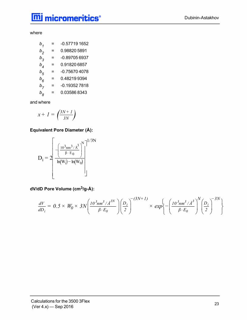
Γ is calculated by a polynomial approximation over the domain 0 ≤ × ≤ 1:

( ) ( )x + 1 = 1 + b x + b x + b x + b x + b x + b x + b x + b x + ϵx ϵx ≤ 3 10Γ 1 22

33

44

55

66

77

88 −7

1 ) Ross andOlivier, J.P., “On Physical Adsorption,” J. Wiley and Sons, New York (1964).

Dubinin-Astakhov


where

b1 = -0.57719 1652b2 = 0.98820 5891b3 = -0.89705 6937b4 = 0.91820 6857b5 = -0.75670 4078b6 = 0.48219 9394b7 = -0.19352 7818b8 = 0.03586 8343

and where

( )x + 1 =3N + 1

3N

Equivalent Pore Diameter (Å):

⋅

( ) ( )D = 2i

−

ln W − ln W

1/3N

103nm3 / Å3

β E0

N

i 0

dV/dD Pore Volume (cm3/g-Å):

⋅ ⋅= 0.5 × W × 3N × exp −dV

dD 010 nm / Å

β E

D

2

−(3N+1)10 nm / Å

β E

ND

2

−3N

i

3 3 3N

0

i3 3 3

0

i

Dubinin-Astakhov


DUBININ-RADUSHKEVICHTheDubinin-Radushkevich1 ) equation is:

log Q = log Q0−BT

β× log

P

P

22

0

where

β = the affinity coefficient of analysis gas relative to P0 gas (for this application β is takento be 1)

B = a constantP0 = saturation vapor pressure of gas at temperature TP = equilibrium pressureQ = quantity adsorbed at equilibrium pressure (cm3/g STP)Q0 = themicropore capacity (cm3/g STP)T = analysis bath temperature (K), from theP0 and Temperature Optionswindow

For each point designated for Dubinin-Radushkevich calculations, the following calculations aredone:

LV = log(Q )

( )LP = logP

P

20

The intercept, log(Vo) can be found by performing a least-squares fit on the (LP,LV) designatedpairs where LP is the independent variable and LV is the dependent variable. Assuming theadsorption of gas is restricted to amonolayer,Vo is themonolayer capacity. Based on thisassumption, the following are calculated:

1 ) Dubinin, M.,Carbon 21, 359 (1983); Dubinin, M., Progress in Surface andMembrane Science 9,1, Academic Press, New York (1975); Dubinin, M. and Astakhov, V., Adv. Chem. Ser. 102, 69(1971); Lamond, T. andMarsh, H.,Carbon 1, 281, 293 (1964); Medek, J., Fuel 56, 131 (1977);Polanyi, M., Trans. Faraday Soc. 28, 316 (1932); Radushkevich, L., Zh. fiz. Kemi. 33, 2202 (1949);Stoeckli, H., et al, Carbon 27, 125 (1989).

Dubinin-Radushkevich


a. Slope (S cm3/g STP)b. Y-intercept (YI cm3/g STP)c. Error of the slope (Serr cm

3/g STP)d. Error of the y-intercept (YIerr cm



Monolayer Capacity (cm3/g STP):

Q = 100

YI

Error of Monolayer Capacity (cm3/g STP):

( )Q = Q 10 − 1.00, err 0

YI, err

Micropore surface area (m2/g):

SDP =σ Q N

22414cm

0 A

3 1018 nm2

m2

where

σ = molecular cross sectional area of gas (nm2) from theAdsorptive Propertieswindow

Dubinin-Radushkevich


EQUATION OF STATEThe ideal gas law relates pressure, volume, temperature, and quantity of gas

where

P = pressureR = a constant that depends on the units of n

For n in cm3, STPR =

P

T

STD

STD

For n in moles,R = 8.3145 Jmol-1 K-1

T = temperatureV = volumez = compressibility factor for the gas at the given pressure and temperature

The real gas equation of state

n =PV

RTz(P, T )

Equation of State


EQUILIBRATIONEquilibration is reached when the pressure change per equilibration time interval (first derivative) isless than 0.01% of the average pressure during the interval. Both the first derivative and averagepressure are calculated using the Savitzky-Golay1 ) convolutionmethod for polynomial functions.The following equations are those used to compute weighted average and first derivative,respectively, for the 6th point of an 11-point window.

P =avg−36(P + P ) + 9(P + P ) + 44(P + P ) + 69(P + P ) + 84(P + P ) + 89(P )

429

11 1 10 2 9 3 8 4 7 5 6

P =chg5(P − P ) + 4(P − P ) + 3(P − P ) + 2(P − P ) + (P − P )

110

11 1 10 2 9 3 8 4 7 5

P = 100%pcp,i

P

P

chg

avgpressure change per equilibration time interval

where the numerical constants are from the Savitzky-Golay convolution arrays, and

Pavg = average pressurePchg = change in pressurePpcp,i = percent change per intervalPi = ith pressure reading taken at equilibrium intervals

If a non-zero value that is too small is entered for themaximumequilibration time, thepoints are collected before equilibration is reached.

If Pavg is greater than 0.995 times the currentP0, equilibration will not take place untiltheMinimumequilibration delay for P/P0 0.995 has expired, in addition to the standardequilibration criteria.

1 ) Savitzky, A. andGolay, M.J.E.,Anal. Chem. 36, 1627 (1964).

Equilibration


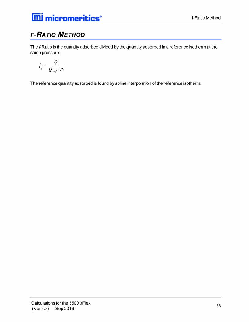
F-RATIO METHOD

The f-Ratio is the quantity adsorbed divided by the quantity adsorbed in a reference isotherm at thesame pressure.

ƒ =i

Q

Q P

i

ref i

The reference quantity adsorbed is found by spline interpolation of the reference isotherm.

f-Ratio Method


FIRST ORDER KINETICS FOR TCDHeat of desorption is calculated from experiments with different temperature ramp rates. Thegeneral equation is

= − +ln ln

β

T

E

RT

E Q

RCp2

d

p

d s

Heat of desorption is proportional to the slope s of 2 lnTp−ln β vs 1/Tp.

E = sRd

The slope is determined by a least-squares fit.

where

β = ramp rate in K/minEd = heat of desorption in kJ/molR = ideal gas constantTp = temperature at peakmaximums = slope of best-fit lineQs = quantity adsorbed at saturationC = constant related to the desorption rate

First Order Kinetics for TCD


FREE SPACE FOR CHEMICAL ADSORPTIONThe free space is the physical volume below the sample valve. The different temperatures in thesample tube, stem, and port must be accounted for.

Free space volumes are calculated as:

( )n =p

PV

z P, T T

s p

s p p

n = n − ns d p

V =sn z(P , T )T

P

s s s s

s

The reported free space is

V = V + Vf p s

The quantity of gas in the free space for a given data point is:

( )

n = P +p s

V

z P , T T

V

z(P , T , )T

p

s p p

s

s s s

where

nd = quantity of gas dosednp = quantity of gas in the portns = quantity of gas in the sample tubePs = sample (and port) pressureTp = port temperatureTs = sample temperatureVp = volume of the sample portVs = volume of the sample tubez(P,T) = gas compressibility factor P and temperature T for the gas used

Free Space for Chemical Adsorption


FREUNDLICH ISOTHERMThe Freundlich isotherm has the form:

= CPQ

Q

1m

m

where

C = temperature-dependent constantm = temperature-dependent constantP = equilibrated collected pressuremeasured by gauge at temp TambQ = quantity of gas adsorbedQm = quantity of gas in amonolayer

The pressure is absolute; typically, m > 1. In terms of quantity adsorbed,

Q = Q CPm

1m

Taking the log of both sides yields

log Q = logQ C + log Pm

1

m

Freundlich Isotherm


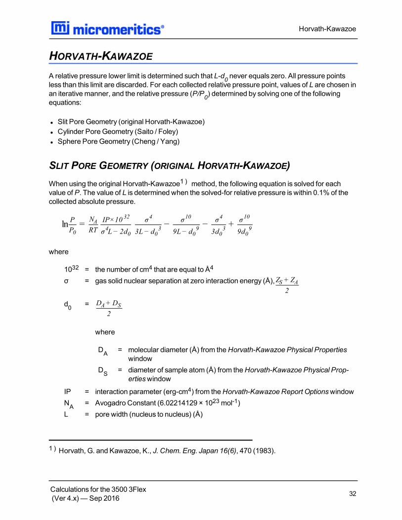
HORVATH-KAWAZOE

A relative pressure lower limit is determined such that L-d0 never equals zero. All pressure pointsless than this limit are discarded. For each collected relative pressure point, values of L are chosen inan iterativemanner, and the relative pressure (P/P0) determined by solving one of the followingequations:

l Slit Pore Geometry (original Horvath-Kawazoe)l Cylinder Pore Geometry (Saito / Foley)l Sphere Pore Geometry (Cheng / Yang)

SLIT PORE GEOMETRY (ORIGINAL HORVATH-KAWAZOE)When using the original Horvath-Kawazoe1 ) method, the following equation is solved for eachvalue of P. The value of L is determined when the solved-for relative pressure is within 0.1% of thecollected absolute pressure.

= − − +lnP

P

N

RT

IP×10

σ L− 2d

σ

3L − d

σ

9L− d

σ

3d

σ

9d0

A32

4

0

4

0

3

10

0

9

4

0

3

10

0

9

where

1032 = the number of cm4 that are equal to Å4

σ = gas solid nuclear separation at zero interaction energy (Å),Z + Z2

S A

d0 = D +D

2

A S

where

DA = molecular diameter (Å) from theHorvath-Kawazoe Physical Propertieswindow

DS = diameter of sample atom (Å) from theHorvath-Kawazoe Physical Prop-ertieswindow

IP = interaction parameter (erg-cm4) from theHorvath-Kawazoe Report OptionswindowNA = Avogadro Constant (6.02214129 × 1023mol-1)L = pore width (nucleus to nucleus) (Å)

1 ) Horvath, G. and Kawazoe, K., J. Chem. Eng. Japan 16(6), 470 (1983).

Horvath-Kawazoe


P = equilibrium pressureP0 = saturation pressureR = gas constant (8.31441 × 107 erg/molK)T = analysis bath temperature (K), from an entered or calculated value on theP0 and

Temperature Optionswindow

where:

Zs = sample equilibrium diameter at zero interaction energy (Å) from theHor-vath-Kawazoe Physical Propertieswindow

ZA = zero interaction energy diameter from theHorvath-Kawazoe PhysicalPropertieswindow

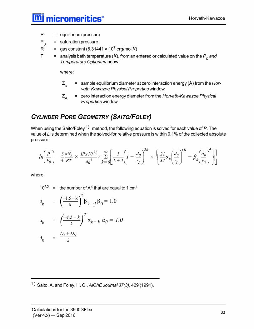
CYLINDER PORE GEOMETRY (SAITO/FOLEY)When using the Saito/Foley1 ) method, the following equation is solved for each value of P. Thevalue of L is determined when the solved-for relative pressure is within 0.1% of the collected absolutepressure.

ln = × × 1 − × α − βΣ

P

P

3

4

πN

RT

IPx10

d k =0

∞1

k + 1

d

r

2k21

32 kd

r

10

k

d

r

4

0

A32

04

0 0 0

where

1032 = the number of Å4 that are equal to 1 cm4

βk = ( ) β , β = 1.0−1.5 − k

k

2

k−1 0

αk = ( ) α , α = 1.0−4.5 − k

k

2

k−1 0

d0 =D +D

2

A S

1 ) Saito, A. and Foley, H. C., AlChE Journal 37(3), 429 (1991).

Horvath-Kawazoe


where



IP = interaction parameter (10-43 erg-cm4) from theHorvath-Kawazoe Report Optionswin-dow

NA = Avogadro Constant (6.02214129 × 1023mol-1)

L = pore width (nucleus to nucleus) (Å)

P = equilibrium pressure

Po = saturation pressure

R = gas constant (8.31441 × 107 erg/molK)

rp = radius of the cylindrical pore,L

2

T = analysis bath temperature (K), from an entered or calculated value on thePo and Tem-perature Optionswindow

Horvath-Kawazoe


SPHERE PORE GEOMETRY (CHENG/YANG)When using the Cheng / Yang1 ) method, the following equation is solved for each value of P. Thevalue of L is determined when the solved-for relative pressure is within 0.1% of the collected absolutepressure.

ln = − + + +

P

P

6N ε* + N ε * L ×10

RTL− d

d

L

6

T

12

T

8

d

L

12

T

90

T

800

1 12 2 22

3 32

0

3

0 1 2 0 3 4

where

1032 = the number of cm4 that are equal to Å4

ε*12 =( )

, whereÅ =Å

4ds

6 mc α α

+

S

s

6

2

S A

αS

χS

αA

χA

ε*22 =( )( )( )

, where Å =A

4DA

3 mc α χ

2

A

A6

2A A

d0 =D + D

2

A S

where



L = pore width (nucleus to nucleus) (Å)

N1 = 4π L2NS, whereNs = number of sample atoms/cm2 at monolayer

N2 = 4π (L-d0)2NA, where NS = number of gasmolecules/cm

2

P = equilibrium pressure

P0 = saturation pressure

R = gas constant (8.31441 × 107 erg/mol K)

1 ) Cheng, Linda S. and Yang, Ralph T.,Chemical Engineering Science 49(16), 2599-2609 (1994).

Horvath-Kawazoe


T = analysis bath temperature (K), from an entered or calculated value on theP0 and Tem-perature Optionswindow

( ) ( )T = −1

1

1 − S

1

1 + S3 3

( ) ( )T = −2

1

1 + S

1

1 − S2 2

( ) ( )T = −3

1

1 − S

1

1 + S9 9

( ) ( )T = −4

1

1 + S

1

1 − S8 8

whereS =

L− d

L

0

CHENG/YANG CORRECTIONThis factor corrects for the nonlinearity of the isotherm. It adds an additional term to the equations forthe different geometrics:

ln = G L − 1 − lnP

P

1

θ

1

1 − θ0

where

G(L) = one of the Horvath-Kawazoe equations given aboveθ = degree of void filling; θ is estimated by first computing themonolayer capacity (Qm)

with the Langmuir equation over the range of data points from relative pressure0.02 to 0.2 or themaximum relative pressure included in the Horvath-Kawazoe ana-lysis. θ is computed as the quantity adsorbed overQm.

Horvath-Kawazoe


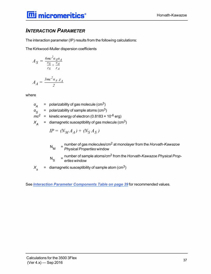
INTERACTION PARAMETERThe interaction parameter (IP) results from the following calculations:

The Kirkwood-Muller dispersion coefficients

A =S6mc α α

+

2

S A

αS

χS

αA

χA

A =A

3mc α χ

2

2A A

where

αA = polarizability of gasmolecule (cm3)αS = polarizability of sample atoms (cm3)mc2 = kinetic energy of electron (0.8183 × 10-6 erg)ΧA = diamagnetic susceptibility of gasmolecule (cm3)

IP = (N A ) + (N A )M A S S

NM = number of gasmolecules/cm2 at monolayer from theHorvath-KawazoePhysical Propertieswindow

NS = number of sample atoms/cm2 from theHorvath-Kawazoe Physical Prop-ertieswindow

Χs = diamagnetic susceptibility of sample atom (cm3)

See Interaction Parameter Components Table on page 39 for recommended values.

Horvath-Kawazoe


ADDITIONAL CALCULATIONSBased on the previous calculations, the following can be calculated:

Adjusted Pore Width (Å):

(Shell to Shell)

AL = L − Di i S

Cumulative Pore Volume (cm3/g):

V =cum,i

Q V

22414cm STP

i mol

3

where

Vmol = liquidmolar volume from the fluid property information

dV/dD Pore Volume (cm3/g-Å):

=dV

dD

V − V

AL − ALi

cum,i cum,i−1

i i−1

Median Pore Width (Å):

V =half

V

2

cum,n

D = exp ln D + (ln D − lnD )ι g ι

ln V − ln V

ln V − ln Vmedg ι

half ι

where

D1 = pore width (Li) that corresponds toVιDg = pore width (Li) that corresponds toVgVcum,n = total cumulative pore volume (Vcum,i) for points designated for Horvath-Kawazoe

calculationsVg = cumulative pore volume (Vcum,i) for first point greater thanVhalfVhalf = 50% of total cumulative pore volumeVl = cumulative pore volume (Vcum,i) for first point less thanVhalf

Horvath-Kawazoe


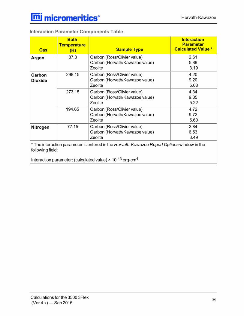
Gas

BathTemperature

(K) Sample Type

InteractionParameter

Calculated Value *

Argon 87.3 Carbon (Ross/Olivier value)Carbon (Horvath/Kawazoe value)Zeolite

2.615.893.19

CarbonDioxide

298.15 Carbon (Ross/Olivier value)Carbon (Horvath/Kawazoe value)Zeolite

4.209.205.08


4.349.355.22


4.729.725.60

Nitrogen 77.15 Carbon (Ross/Olivier value)Carbon (Horvath/Kawazoe value)Zeolite

2.846.533.49

* The interaction parameter is entered in theHorvath-Kawazoe Report Optionswindow in thefollowing field:

Interaction parameter: (calculated value) × 10-43 erg-cm4

Interaction Parameter Components Table

Horvath-Kawazoe


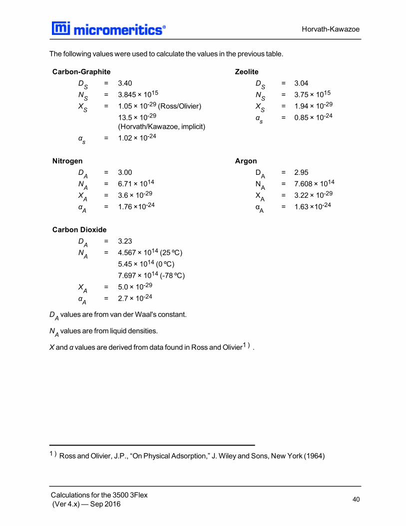
The following valueswere used to calculate the values in the previous table.

Carbon-Graphite ZeoliteDS = 3.40 DS = 3.04NS = 3.845 × 1015 NS = 3.75 × 1015

XS = 1.05 × 10-29 (Ross/Olivier) XS = 1.94 × 10-29

13.5 × 10-29(Horvath/Kawazoe, implicit)

αs = 0.85 × 10-24

αs = 1.02 × 10-24

Nitrogen ArgonDA = 3.00 DA = 2.95NA = 6.71 × 1014 NA = 7.608 × 1014

ΧA = 3.6 × 10-29 XA = 3.22 × 10-29

αA = 1.76 ×10-24 αA = 1.63 ×10-24

Carbon DioxideDA = 3.23NA = 4.567 × 1014 (25 ºC)

5.45 × 1014 (0 ºC)7.697 × 1014 (-78 ºC)

XA = 5.0 × 10-29

αA = 2.7 × 10-24

DA values are from van der Waal's constant.

NA values are from liquid densities.

Χ and α values are derived from data found in Ross andOlivier1 ) .

1 ) Ross andOlivier, J.P., “On Physical Adsorption,” J. Wiley and Sons, New York (1964)

Horvath-Kawazoe


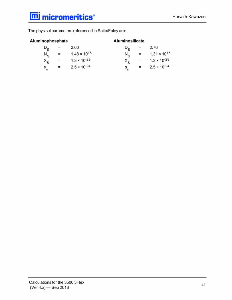
The physical parameters referenced in Saito/Foley are:

Aluminophosphate AluminosilicateDS = 2.60 DS = 2.76NS = 1.48 × 1015 NS = 1.31 × 1015

XS = 1.3 × 10-29 XS = 1.3 × 10-29

αs = 2.5 × 10-24 αs = 2.5 × 10-24

Horvath-Kawazoe


INJECTION LOOP CALIBRATION FOR TCD

Q = Ql s

A

A

l

s

The effective loop volume at 0 °C is

V = Ql, l,STP

P

PeffSTD

l

= Qs,STP

A

A

T

T

l

s

i

a

where

Ql = quantity of gas in loop injectionQs = quantity of gas in syringe injectionAl = peak area from loop injectionAs = peak area from syringe injectionTl = temperature of loop in kelvins

Injection Loop Calibration for TCD


LANGMUIR SURFACE AREA FOR CHEMICAL ADSORPTION

TRANSFORM FOR CHEMICAL ADSORPTIONThe Langmuir isotherm is

=Q

Q

bP

1 + bPm

The isotherm is transformed so that P/Q is plotted as a function of pressure. The transformed dataare fitted with a straight line. the slope (m) and intercept (y0) of the fit line are used in the calculationsbelow.

SURFACE AREA

⋅A = 10LangA SN

V m

−18 m

nm

atom A

mol

2

2

MONOLAYER CAPACITYQm=

1m

LANGMUIR b VALUE

b =1

y Q0 m

DISSOCIATIVE CHEMICAL ADSORPTIONThe Langmuir isothermmay be derived for dissociative chemical adsorption.

=Q

Q

b P

1 + b Pm

The calculations are performedwith the slope and intercept of a fit of

P

Q as a function of P .

Langmuir Surface Area for Chemical Adsorption


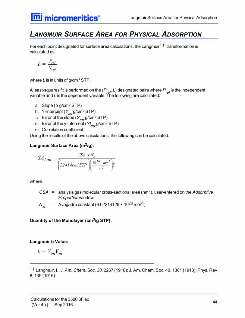
LANGMUIR SURFACE AREA FOR PHYSICAL ADSORPTIONFor each point designated for surface area calculations, the Langmuir1 ) transformation iscalculated as:

L =P

N

rel

ads

where L is in units of g/cm3 STP.

A least-squares fit is performed on the (Prel, L) designated pairs wherePrel is the independentvariable and L is the dependent variable. The following are calculated:

a. Slope (S g/cm3 STP)b. Y-intercept (Yint g/cm

3 STP)c. Error of the slope (Serr g/cm

3 STP)d. Error of the y-intercept (YIerr g/cm

3 STP)e. Correlation coefficient


Langmuir Surface Area (m2/g):

SA =Lan

CSA x N

22414cm STP S

A

3 1018

nm2

m2

where

CSA = analysis gasmolecular cross-sectional area (nm2), user-entered on theAdsorptivePropertieswindow

NA = Avogadro constant (6.02214129 × 1023mol-1)

Quantity of the Monolayer (cm3/g STP):

Langmuir b Value:

b = Y Vint m

1 ) Langmuir, I., J. Am. Chem. Soc. 38, 2267 (1916); J. Am. Chem. Soc. 40, 1361 (1918); Phys. Rev8, 149 (1916).

Langmuir Surface Area for Physical Adsorption


Error of the Langmuir Surface Area (m2/g):

LAN =err

SA S

S

Lan err

Langmuir Surface Area for Physical Adsorption


LANGMUIR SURFACE AREA FOR TCDSurface area is calculated as the number of molecules in themonolayer times the area of amolecule.The result is divided by samplemass to give the specific surface area.

A = Q N A / mLang m,mol, A α

The quantity of adsorbate in themonolayer is determined by fitting Langmuir-transformed data frommultiple experiments.

L =iP

Q

i

i

P = c Pi i 0

The slope s and offset y0 of the best-fit line through Li vs. Pi are found.

Q = 1 / sm

b = y / s0

Uncertainty in the surface area is estimated from the uncertainty in the slope.

u(A ) = ALang Langu(s)

s

where

ALang = specific Langmuir surface areaQm,mol = quantity of adsorbate in themonolayer in molesNA = Avogadro constant: 6.02214129 × 1023mol-1

Aα = adsorbate cross-sectional aream = samplemassLi = Langmuir transform for experiment iPi = absolute pressure from experiment iQi = cumulative quantity adsorbed for all peaks in experiment ici = active gas concentration in experiment ib = Langmuir b valueP0 = entered saturation pressure for the active gas

Langmuir Surface Area for TCD


s = slope of best-fit liney0 = intercept of best-fit lineu(x) = uncertainty of x

Langmuir Surface Area for TCD


METAL DISPERSION FOR CHEMICAL ADSORPTION

⋅D = 100% 100%Q S

V Σ

o

mol

Pi

Wi

where

≃V 22414cm / molmol

3 = themolar volume of an ideal gas at standard tem-perature and pressure

Metal Dispersion for Chemical Adsorption


METALLIC SURFACE AREA FOR CHEMICAL ADSORPTIONThemetallic surface area is the total activemetal surface area available for interaction with theadsorbate.

A =metal

N Q SA

V

A o atom

mol

where

≃N 6.023 × 10A

23 = the number of atoms per mole

Metallic Surface Area for Chemical Adsorption


METALLIC SURFACE AREA FOR TCDA = Q SA N / mmetal α,mol cs A

where

Qa,mol = cumulative quantity adsorbed inmolesS = weighted stoichiometry factorAcs = weighted atomic cross-sectional areaNA = Avogadro constant: 6.02214129 × 1023mol-1

m = samplemass

Metallic Surface Area for TCD


MP-METHOD

With the (ti,Qi) data pairs1 ) , the Akima semi-spline interpolationmethod is used to interpolate

quantity adsorbed values based on thickness values that are evenly spaced 0.2 angstrom apartstarting at the first outlier point. Outliers are defined as those points that have themaximuminstantaneous slope within an iteratively shrinking subset of all points. The remaining pore surfacearea calculation result is the slope of the line defined by two consecutive interpolated points. Theslopes of each pair of consecutive points from the origin to the last point must bemonotonicallydecreasing and non-negative. With the interpolated points set the following can be calculated:

Average pore hydraulic radius (Å):

R =it + t

2

i i−1

Remaining pore surface area for the ith point (m2/g):

S = × 10i

Q −Q

t − t

V

22414 cm STP

4i i−1

i i−1

mol

3

where

104 = unit conversionsVmol = liquidmolar volume from the fluid property information

Incremental pore surface area occluded for the ith point (m2/g):

S = S − Sinc,i i−1 i

Cumulative pore surface area occluded for the ith point (m2/g):

S = S + S +…+ Scum inc, i inc, i−1 inc, ii

dA/dR pore surface area for the ith point (m2/g-Å):

=dA

dR

S

t − t1

inci

i i−1

1 ) Mikhail, R., Brunauer, S. and Bodor, E., J. Colloid and Interface Sci. 24, 45 (1968).

MP-Method


Incremental pore volume occluded for the ith point (cm3/g):

V = S R × 10inc, i inc, i i−4

Cumulative pore volume occluded for the ith point (cm3/g):

V = V + V +…+ Vcum, i inc, i−1 inc, i

dV/dR pore volume for the ith point (cm3/g-Å):

=dV

dR

V

t − ti

inc, i

i i−1

MP-Method


PARTICLE SIZE FOR TCDSeeCrystallite Size for Chemical Adsorption on page 14 .

Particle Size for TCD


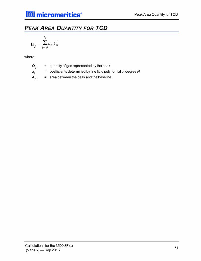
PEAK AREA QUANTITY FOR TCD

ΣQ = a Ap

i=0

N

i pi

where

Qp = quantity of gas represented by the peakai = coefficients determined by line fit to polynomial of degreeNAp = area between the peak and the baseline

Peak AreaQuantity for TCD


PERCENT DISPERSION FOR TCDD = 100%Q SM / m

α,mol

where

Qα,mol = cumulative quantity adsorbed inmolesS = Stoichiometry factorM = molecular weightm = samplemass

Percent Dispersion for TCD


QUANTITY ADSORBED FOR CHEMICAL ADSORPTIONA portion of the dosing volumemay be at a slightly elevated temperature due to heating of thesample ports. Themanifold volume is partitioned into a volume at the temperature of themanifoldblock and a volume at the average temperature of the ports.

n = n − na d f

( ) ( )n = P C P , T , T − P C P , T , Td 1m 1m 1m 1p 2m 2m 2m 2p

( )

C P, T , T = V +m p mα

z(P, T )T

β

z P, T Tm m p p

where

ɑ and β = constants that determine the relative weights of themanifold and port tem-peratures

nɑ = quantity of gas adsorbednd = quantity of gas dosednf = quantity of gas in the free spaceP1m = manifold pressure before dosing onto the sampleP2m = manifold pressure after dosingT1m = manifold temperature before dosing onto the sampleT1p = average of all port temperatures before dosing onto the sampleT2m = manifold temperature after dosingT2m = average of all port temperatures after dosingVm = volume of the dosingmanifold

Quantity Adsorbed for Chemical Adsorption


QUANTITY ADSORBED FOR PHYSICAL ADSORPTIONFor the ith dose, the quantity dosed is

( ) ( )n(i ) = n + n P , V , T − n P , V , Tdosed,i dosed,i−1 1 m 1 2 m 2

The pressure, volume, and temperature are those of the dosingmanifold before and after expandinginto the sample tube.

n = n − nads,i dosed,i fs,i

The quantity of gas in the free space is

( ) ( )

n = +fs, i

P

T

V

z P , T

V

z P , T

s,i

STD

bath

s,i bath

amb

s,i amb

with the real gas equation of state. Here,Ps is the sample pressure.

The specific quantity adsorbed is

Q =ads,i

n

m

ads,i

V =bath

V − V

1 −

fc fw

T bath

Tamb

Quantity Adsorbed for Physical Adsorption


FREE SPACE - MEASURED

Measured free-space volumes are calculated using the following equations:

V = − 1 TfwV

T

P

P STDman

man

1

2

V = Vfc fwP

P

2

3

FREE SPACE - CALCULATEDThe calculated free space is determined by subtracting the gas capacity of the volume occupied bythe sample from themeasured free space of the empty tube.

V = V − Vfw wb sT

T

STD

amb

V =bath

V − V

1 −

fc fw

T bath

Tamb

V =sm

ρ



COMPENDIUM OF VARIABLES

ρ = sample density

m = samplemass

Pi = equilibrated sample pressure

P1 = systemmanifold pressure before dosing onto sample

P2 = systemmanifold pressure after dosing onto sample

P3 = sample pressure after raising dewar and equilibrating with helium

Tamb = approximate room temperature (298 K)

Tbath = analysis bath temperature (K)

Tman = systemmanifold temperature before dosing helium onto sample (K)

TSTD = standard temperature (273.15 K)

Vamb = volume of cold free space (cm3 at standard temperature)

Vbath = volume of cold free space at analysis bath temperature (cm3 at standardtemperature)

Vcb = volume of cold free space of the empty tube (cm3 at standard temperature)

Vfc = volume of cold free space (cm3 at standard temperature)

Vfw = volume of warm free space (cm3 at standard temperature)

Vman = manifold volume (cm3)

Vs = sample volume

Vwb = volume of warm free space of the empty tube (cm3 at standard temperature)



QUANTITY ADSORBED FOR TCDThe quantity adsorbed is the amount of gas removed from a loop or syringe injection by the sample.

Q = NQ − Qα i n

where

Qα = quantity adsorbedN = number of injectionsQi = injection quantityQn = quantity detected, not adsorbed

Quantity Adsorbed for TCD


QUANTITY OF GAS FOR TCDThe quantity of gas in an injection is found by the equation of state. In moles

Q = Vmol

P

zRT

α

α

In cm3 at standard temperature and pressure (cm3 STP)

Q = VSTP

P

zT

T

P

α

α

STD

STD

where

V = volume in cm3

Pα = entered atmospheric pressurez = compressibility factor at Pα and Tα for the injected gasTα = entered ambient temperature in kelvinsR = ideal gas constantTSTD = standard temperature: 273.15 KPSTD = standard pressure: 101.325 kPa, 760mmHg

Quantity of Gas for TCD


REAL GAS EQUATION OF STATE FOR CHEMICALADSORPTIONAll chemical adsorption gas accounting calculations utilize the real gas equation of state andcompressibility factor data traceable to NIST.

n =PV

z(P, T )T

where

n = quantity of gasP = pressureT = temperatureV = volumez(P,T) = compressibility factor for the gas of interest at the given pressure and tem-

perature

Quantity of gas in cm3 STP is given by

Q = nT

P

STD

STD

Real Gas Equation of State for Chemical Adsorption


RELATIVE PRESSUREIf P0 is measured in theP0 tube, the current pressure ismeasured in theP0 tube when each point istaken, and used to calculate relative pressure for that point:

P =rel

P

Po

Relative Pressure


SATURATION PRESSURESaturation pressure (P0) is selected on theP0 and Temperature Optionswindow. It may be enteredor measured in the P0 tube. The analyzer uses the followingmethods to get P0:

1. P0 is measured in the P0 tube for each isotherm point.2. The saturation pressure ismeasured in the sample tube after all adsorption data points have

been collected. This pressure is used as P0 for all data points.3. P0 is measured for all points aswith #1. After all adsorption points have been taken P0 is meas-

ured in the sample tube. Themeasured P0 points are shifted so that the P0measured in theP0 tubematches the P0measured in the sample tube. That is, Poi = Poi + Pos - Pon wherePon is the P0measured in the P0 tube when P0 in the sample tube (Pos) wasmeasured.

4. Determine P0 from pressuremeasured over the dosing source. Note that theAdsorptive Prop-ertiesmust specify dosing fromPsat tube, Sample port 3, or Vapor source.

5. The saturation pressure of a gas ismeasured in the P0 tube for each data point. The bath tem-perature is found by looking up the temperature for themeasured saturation pressure in thefluid properties. P0 of the analysis gas is found from the bath temperature as in #6. If dosing isdone from the Psat tube, P0 is determined once at the beginning of the analysis and used forall data points. Otherwise, P0 is measured for each data point.

6. P0 is found by looking up the saturation pressure for the entered bath temperature in the fluidproperty information.

Lookup of saturation pressure in the fluid properties is done by interpolating the Psat data

using the Clausius-Clapeyron equation,

ln P =

α

T+ b

. The constants α and b aredetermined from the pressures and temperatures that bound the bath temperature.

Temperature lookup is done by solving for T,T =

α

ln(P ) − b , where α and b are determinedfrom the pressures that bound the given saturation pressure.

7. If entered, P0 = user-entered value.

Saturation Pressure


SPC REPORT VARIABLES

REGRESSION CHART VARIABLESThe line of best fit for the Regression Chart is calculated by the usual least squaresmethod. 1 ) Ifthere is only a single point or allN points have the same x-value, there can be no line of best fit in thestandard form.

χ =χ

N

Σi

y =y

N

Σi

( )( )( )

Slope =χ − χ y − y

χ − χ

Σ

Σ

i i

i2

⋅Intercept = y − xSlope

The coefficient of correlation for this line is also calculated in the usual way. 2 )

( )σ =χ

χ − χ

N

Σi

2

( )σ =y

y − y

N

Σi

2

( )( )(x, y ) =Cov

x − x y − y

N

Σ i i

Correlation Coeff =(x, y )

σ σ

Cov

x y

1 ) BASIC Scientific Subroutines Vol II, by F.R. Ruckdeschel, Copyright 1981 BYTEPublications/McGraw Hill, p. 16.2 ) Mathematical Handbook for Scientists and Engineers, G.A. Korn and T.M. Korn, McGraw Hill,Sec. 18.4. (1968)

SPC Report Variables


CONTROL CHART VARIABLES

Mean =y

N

Σi

( )Standard Deviation =

y −

N − 1

Σ Meani

2

C. V.=StdDev

Mean

⋅+ n σ = Mean + n Standard Deviation

⋅− n σ = Mean − n Standard Deviation

SPC Report Variables


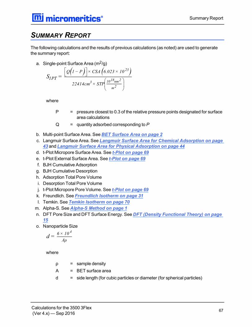
SUMMARY REPORTThe following calculations and the results of previous calculations (as noted) are used to generatethe summary report:

a. Single-point Surface Area (m2/g)

( ) ( )S =1PT

Q 1 − P ×CSA 6.023 × 10

22414cm × STP

23

3 1018nm2

m2

where

P = pressure closest to 0.3 of the relative pressure points designated for surfacearea calculations

Q = quantity adsorbed corresponding toP

b. Multi-point Surface Area. SeeBET Surface Area on page 2c. Langmuir Surface Area. See Langmuir Surface Area for Chemical Adsorption on page

43 and Langmuir Surface Area for Physical Adsorption on page 44d. t-Plot Micropore Surface Area. See t-Plot on page 69e. t-Plot External Surface Area. See t-Plot on page 69f. BJH Cumulative Adsorptiong. BJH Cumulative Desorptionh. Adsorption Total Pore Volumei. Desorption Total Pore Volumej. t-Plot Micropore Pore Volume. See t-Plot on page 69k. Freundlich. See Freundlich Isotherm on page 31l. Temkin. See Temkin Isotherm on page 70

m. Alpha-S. SeeAlpha-S Method on page 1n. DFT Pore Size and DFT Surface Energy. SeeDFT (Density Functional Theory) on page

15o. Nanoparticle Size

d =6 × 10

Aρ

4

where

ρ = sample densityA = BET surface aread = side length (for cubic particles or diameter (for spherical particles)

SummaryReport


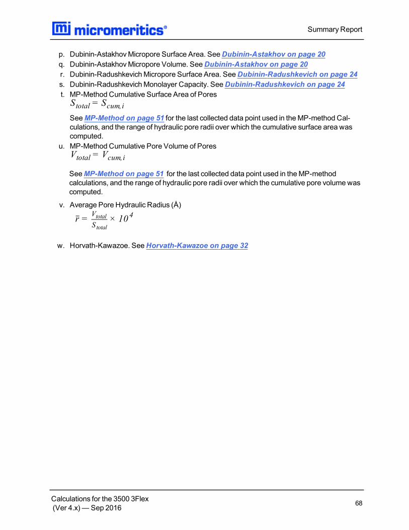
p. Dubinin-AstakhovMicropore Surface Area. SeeDubinin-Astakhov on page 20q. Dubinin-AstakhovMicropore Volume. SeeDubinin-Astakhov on page 20r. Dubinin-RadushkevichMicropore Surface Area. SeeDubinin-Radushkevich on page 24s. Dubinin-RadushkevichMonolayer Capacity. SeeDubinin-Radushkevich on page 24t. MP-Method Cumulative Surface Area of PoresS = Stotal cum,i

SeeMP-Method on page 51 for the last collected data point used in theMP-method Cal-culations, and the range of hydraulic pore radii over which the cumulative surface area wascomputed.

u. MP-Method Cumulative Pore Volume of PoresV = Vtotal cum,i

SeeMP-Method on page 51 for the last collected data point used in theMP-methodcalculations, and the range of hydraulic pore radii over which the cumulative pore volumewascomputed.

v. Average Pore Hydraulic Radius (Å)

r = × 10V

S

4total

total

w. Horvath-Kawazoe. SeeHorvath-Kawazoe on page 32

SummaryReport


T-PLOTA least-squares analysis fit is performed on the (ti,Nads,i) data pairs where ti is the independentvariable andNads,i is the dependent variable. Only the values of ti between tmin and tmax, theminimumandmaximum thickness, are used. The following are calculated:

a. Slope (S cm3/g-Å STP)b. Y-intercept (Yint cm

3/g STP)c. Error of the slope (Serr cm

3/g-Å STP)d. Error of the Y-intercept (YIerr cm



External Surface Area (m2/g):

× 10SV

F×22414cm STP

4mol

3

where

104 = unit conversionsF = surface area correction factor, user-entered on the t-Plot Report OptionswindowVmol = liquidmolar volume, from the fluid property information

Micropore Surface Area (m2/g):

SA = SA + SAµρ total ext

whereSAtotal is the BET surface area if the user enabled the BET report exclusively, or Langmuirsurface area if the user enabled the Langmuir report exclusively. If neither report has been selected,SAtotal is the BET surface area value calculated using a set of default parameters.

Micropore Volume (cm3 liquid/g):

Y V

22414cm STP

int mol

3

t-Plot


TEMKIN ISOTHERMThe Temkin isotherm has the form:

= ln A P

Q

Q

RT

q α om 0

where

A0 = adjustable constantɑ = adjustable constantP = equilibrium pressuremeasured by gauge at temp Tambq0 = the differential heat of adsorption at zero surface coverageQ = quantity of gas adsorbedQm = quantity of gas in amonolayerR = molar gas constant

8.31441 × 10−3 kJ

molK

T = bath temperature

In terms of quantity adsorbed

Q = lnA + ln P

RTQ

q α 0m

0

Thus, the plot of the natural log of absolute pressure vs. quantity adsorbed yields a straight line with

slope

RTQ

q

m

0 and interceptlnA0

RTQ

q a

m

0 .

Temkin Isotherm


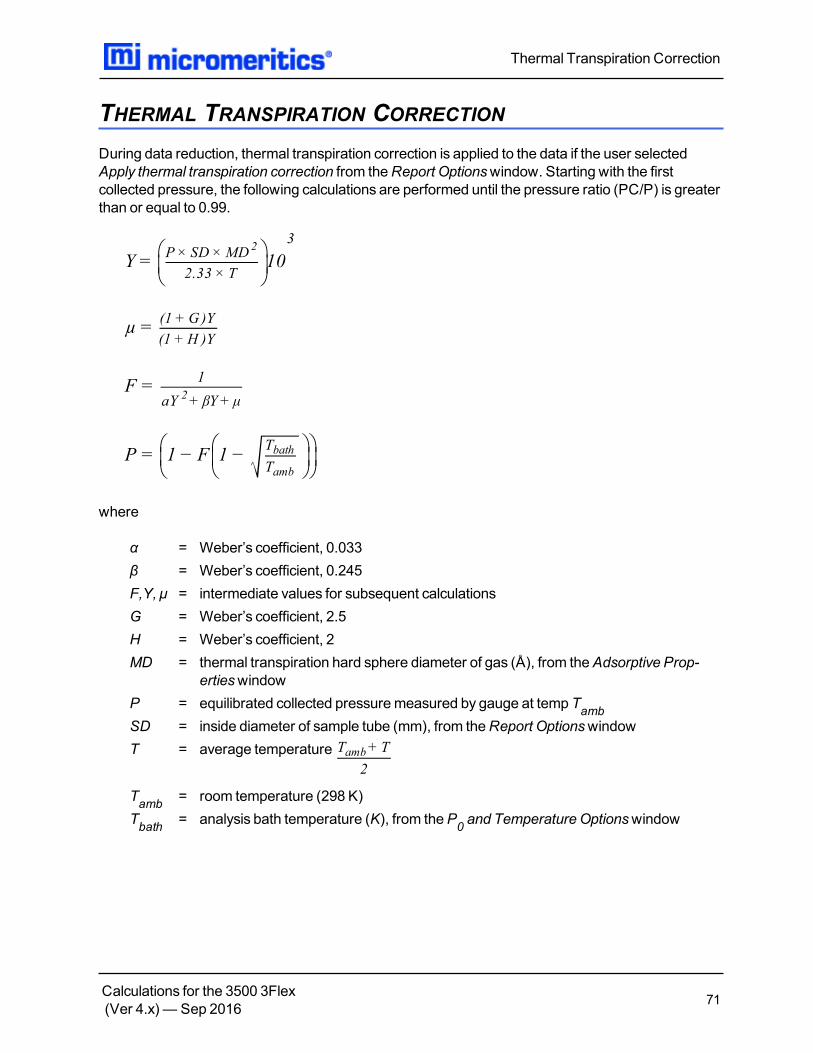
THERMAL TRANSPIRATION CORRECTIONDuring data reduction, thermal transpiration correction is applied to the data if the user selectedApply thermal transpiration correction from theReport Optionswindow. Starting with the firstcollected pressure, the following calculations are performed until the pressure ratio (PC/P) is greaterthan or equal to 0.99.

Y = 10

P× SD ×MD

2.33 × T

32

µ =(1 + G)Y

(1 +H )Y

F =1

aY + βY+ µ2

P = 1 − F 1 −

T

T

bath

amb

where

α = Weber’s coefficient, 0.033β = Weber’s coefficient, 0.245F,Y, µ = intermediate values for subsequent calculationsG = Weber’s coefficient, 2.5H = Weber’s coefficient, 2MD = thermal transpiration hard sphere diameter of gas (Å), from theAdsorptive Prop-

ertieswindowP = equilibrated collected pressuremeasured by gauge at temp TambSD = inside diameter of sample tube (mm), from theReport OptionswindowT = average temperature T + T

2

amb

Tamb = room temperature (298 K)Tbath = analysis bath temperature (K), from theP0 and Temperature Optionswindow

Thermal Transpiration Correction


THICKNESS CURVEFor each point designated, the following parameters are used in thickness curve calculations:

C1 = parameter #1C2 = parameter #2C3 = parameter #3Prel, i = relative pressure for the ith point (mmHg)ti = thickness for ith point

REFERENCEInterpolated from table.

KRUK-JARONIEC-SAYARI

( )

t =C

C = log P

c3

1

2 rel, i

HALSEY

( )

t = Ci 1C

ln P

C

2

rel, i

3 Halsey1 )

HARKINS AND JURA

( )

t =iC

C − log P

C

1

2 rel, i

3 Harkins and Jura2 )

1 ) Halsey, G., J.Chem. Phys. 16, 931-937 (1948).2 ) Harkins, W.D. and Jura, G., J.Chem. Phys. 11, 431 (1943).

ThicknessCurve


BROEKOFF-DE BOER

log P = + C exp c trel, i

C

t , i2 3 i

1

2

CARBON BLACK STSA

( ) ( )t = C P + C P + Ci 1 rel, i

2

2 rel, i 3

ThicknessCurve


WEIGHTED METAL PARAMETERSThe stoichiometry factor, atomic weight, and density used in calculations are averagesweighted bythe number of moles of each activemetal. For example, the average stoichiometry factor is

Σ

ΣS =

n S

n

ii i

ii

where

ni = number of moles or metal

n =iαβX

XW + YWm 0

where

ɑ = fraction of samplemassβ = fraction reducedX = number of metal atoms in the oxideY = number of oxygen atoms in the oxideWm = atomic weight of metalWo = atomic weight of Oxygen

Average density and atomic cross-sectional area are calculated similarly.

WeightedMetal Parameters


Calculations for 3500 3Flex - Micromeritics

Documents

Transcript of Calculations for 3500 3Flex - Micromeritics