An Interval-Parameter Waste-Load-Allocation Model for RiverWater Quality Management Under Uncertainty

Xiaosheng Qin Æ Guohe Huang Æ Bing Chen ÆBaiyu Zhang

Received: 14 April 2008 / Accepted: 12 January 2009 / Published online: 24 February 2009

� Springer Science+Business Media, LLC 2009

Abstract A simulation-based interval quadratic waste

load allocation (IQWLA) model was developed for sup-

porting river water quality management. A multi-segment

simulation model was developed to generate water-quality

transformation matrices and vectors under steady-state

river flow conditions. The established matrices and vectors

were then used to establish the water-quality constraints

that were included in a water quality management model.

Uncertainties associated with water quality parameters,

cost functions, and environmental guidelines were descri-

bed as intervals. The cost functions of wastewater

treatment units were expressed in quadratic forms. A

water-quality planning problem in the Changsha section of

Xiangjiang River in China was used as a study case to

demonstrate applicability of the proposed method. The

study results demonstrated that IQWLA model could

effectively communicate the interval-format uncertainties

into optimization process, and generate inexact solutions

that contain a spectrum of potential wastewater treatment

options. Decision alternatives can be generated by adjust-

ing different combinations of the decision variables within

their solution intervals. The results are valuable for sup-

porting local decision makers in generating cost-effective

water quality management strategies.

Keywords Interval � Quadratic programming �Water quality management � Uncertainty � Optimization

Introduction

Effective planning for water quality management has been

an important task for facilitating sustainable socio-eco-

nomic development in watershed systems. Over the past

decades, many optimization models have been proposed in

this field (Bouwer 2003; Huang and Qin 2008a). The waste-

load-allocation (WLA) model, also named multi-point-

source waste reduction model, is one of the examples that

have been widely used for limiting the amount of waste

discharged into river water systems (Loucks and others

1981, 1985). It is formulated as a problem of minimizing

treatment or pollution abatement costs while specifying a

minimum allowable water quality in the receiving water

bodies (i.e. water quality standards).Water-quality simula-

tion models are normally embedded within a WLA model

framework in order to describe relationships between river

water-quality levels and wastewater control strategies.

However, water quality planning and management are

complicated with a variety of uncertainties (Loucks 2003).

They may be derived from random nature of hydrodynamic

conditions of river systems and meteorological processes,

as well as shortage of available monitoring data (Burn and

X. Qin (&)

Sino-Canada Center of Energy and Environmental Research,

North China Electric Power University, Beijing 102206, China

e-mail: xiaoshengqin@tom.com

X. Qin

Center for Studies in Energy and Environment, University

of Regina, Regina, Saskatchewan S4S 0A2, Canada

G. Huang

Faculty of Engineering, University of Regina, Regina,

Saskatchewan S4S 0A2, Canada

e-mail: huangg@iseis.org

B. Chen

Faculty of Engineering and Applied Science, Memorial

University of Newfoundland, St. John’s, NL A1B 3X5, Canada

B. Zhang

Department of Civil Engineering, Dalhousie University,

1360 Barrington St, Halifax, NS B3J 1Z1, Canada

123

Environmental Management (2009) 43:999–1012

DOI 10.1007/s00267-009-9278-8

McBean 1987; Revelli and Ridolfi 2004; Karmakar and

Mujumdar 2006; Huang and Qin 2008b). In addition,

representation of system costs for water quality manage-

ment involves a number of nonlinear functions for

projecting environmental-economic interrelationships (Qin

and others 2007a). These complexities lead to difficulties in

formulating and solving the resulting nonlinear optimiza-

tion problems.

Previously, efforts were made in dealing with the

uncertainties and nonlinearities in water quality manage-

ment through stochastic, fuzzy and interval mathematical

programs (Huang 1998; Huang and Loucks 2000; Huang

and others 2002; Karmakar and Mujumdar 2006; Liu and

others 2007, 2008). Stochastic programming is a classical

measure for addressing uncertainties in nonlinear water

quality management systems. For example, Fujiwara

(1988) studied the problem of identifying optimal waste

removals to mitigate the impacts of the waste discharges on

the dissolved oxygen (DO) concentration in a water body

through chance-constrained programming method, where

probability of violating the DO deficit standard was

investigated; Dupacova and others (1991) compared three

stochastic programming methods (i.e., approximation,

stochastic quasi-gradient and joint chance-constrained

methods) in applications of a water quality management

problem in Eastern Czechoslovakia; Mujumdar and Saxena

(2004) developed a stochastic dynamic programming

(SDP) model for dealing with waste load allocation (WLA)

problems, where the random variation of streamflows was

included through seasonal transitional probabilities. In

these studies, several modeling parameters were considered

as random variables and described by probability density

functions (PDFs) (Qin and others 2008a). By means of

stochastic analysis such as Monte Carlo simulation, the

problems could be converted into deterministic sub-models

and then solved by traditional nonlinear programming

methods.

Another approach for water quality management under

uncertainty is based on fuzzy set theory. It is a method that

facilitates the analysis of systems with uncertainties being

derived from vagueness or ‘‘fuzziness’’ rather than ran-

domness alone (Qin and others 2007b, 2008b). It is suitable

for situations when the uncertainties cannot be expressed as

probability density functions (PDFs), such that adoption of

fuzzy membership functions becomes an attractive alterna-

tive (Gen and others 1997; Huang and Chang 2003). For

examples, Lee and Wen (1996) evaluated four types of fuzzy

linear programming (FLP) approaches and applied them in

dealing with the allowable pollution loading problems in a

river basin; Sasikumar and Mujumdar (1998) developed a

fuzzy multi-objective optimization model called fuzzy

waste-load allocation model (FWLAM) for water quality

management of a hypothetical river basin; Mujumdar and

Sasikumar (2002) advanced a fuzzy optimization model for

supporting the seasonal water quality management of river

systems, where fuzzy probability approach was used to

reflect risks of violating water quality standards due to

seasonal variations of river flow; Lee and Chang (2005)

proposed an interactive fuzzy approach for handling multi-

objective water quality optimization problems involving

vague and imprecise information related to data, model

formulation, and the decision maker’s preferences.

The stochastic and fuzzy methods have advantages in

their effectiveness in dealing with uncertainties and non-

linearities. However, the stochastic methods are associated

with difficulties in acquiring PDFs for a number of modeling

parameters (Marr 1988); the fuzzy nonlinear programming

methods have been restricted by its complicated mathe-

matical conversions derived from generation of intermediate

models (Wu and others 2006). Interval quadratic program-

ming (IQP) is another alternative for handling both

uncertainty and nonlinearity for optimization problems. The

cost coefficients, constraint coefficients, and right-hand

sides of an IQP model, are represented by interval data.

Since the parameters are interval-valued, the objective value

is interval-valued as well. A pair of two-step mathematical

solution algorithm can be used to calculate the upper bound

and lower bound of the objective values of an interval

quadratic model (Huang and others 1992). The IQP model

will be transformed into a number of deterministic quadratic

programs. Solving these programs produces the intervals of

the objective values and decision variables of the problem.

Applications of IQP have been reported in the field of

solid waste management. For example, Huang and others

(1995) introduced a grey quadratic programming (GQP)

method as a means for municipal solid waste (MSW)

management planning under uncertainty; Wu and others

(2006) proposed an interval quadratic programming model

and applied it to the planning of MSW management system

in the Hamilton-Wentworth Region, Ontario, Canada. The

IQP model is formulated by introducing interval variables

into an ordinary quadratic programming (QP) framework,

and is capable of incorporating uncertainties within the QP

optimization process and the resulting solutions (Huang

and others 1992). Decision alternatives can be obtained by

adjusting decision variables within their solution intervals.

However, applications of IQP model in water quality

management were very limited. Thus, as an extension of

the previous efforts, the objective of this study is to

develop an interval quadratic waste-load-allocation (IQ-

WLA) model for supporting decisions of river water

quality management. A steady-state one-dimensional river

water quality simulation system will be provided to gen-

erate a number of intermediate transformation matrices and

vectors for building the WLP model. Uncertainties related

to water quality parameters will be projected to the

1000 Environmental Management (2009) 43:999–1012

123

optimization model by interval analysis. Nonlinearities and

uncertainties associated with the objective functions will be

handled by formulation of interval quadratic polynomials.

A case study for water quality management planning in the

Xiangjiang river section in Hunan Province, China, will be

used to demonstrate the applicability of the proposed

method.

River Water Quality Simulation

Water quality models are used to address the relationships

between the pollutant loadings and environmental respon-

ses in a stream (or a river), and analyze the potential

impacts of alternative pollution control plans. They have

been used extensively for supporting stream water-quality

management problems over several decades. There are

many different types of water quality models, ranging from

simple models such as Streeter-Phelps, Dobbins and

O’Connor to more sophisticated ones such as QUAL2E and

WASP6 (Rauch and others 1998). In many cases, the

appropriate model and the required data depend on the

purpose of study. Simplifications or assumptions are nor-

mally made in specific planning situations given the limits

of available time and money; in some cases, models should

be relatively simple; in other cases, they may have to be

more complex (Loucks and others 1981). For a typical

WMR problem, the modeling method should be able to

predict the degree of waste removal at various point

sources sites along a water body that will meet both

effluent and water quality standards. In this study, the

O’Connor and Dobbins model is used for supporting

quantification of water quality constraints related to Bio-

logical Oxygen Demand (BOD) and Dissolved Oxygen

(DO) discharges as well as their concentrations in river

waters (O’Connor and Dobbins 1958). A first-order deg-

radation reaction of BOD-DO can be written as:

uxdLc

dt¼ �ðKd þ KsÞLc ð1aÞ

uxdLN

dx¼ �KNLN ð1bÞ

uxdO

dx¼ �kdLc � kNLN þ kaðOs � OÞ; ð1cÞ

where Lc is the ultimate Carbonaceous BOD (CBOD)

concentration, [ML-3]; LN is the ultimate Nitrogenous

BOD (NBOD) concentration, [ML-3]; kd is the CBOD

decay rate in river streams, [T-1]; ks is the CBOD decay

rate due to sedimentation, [T-1]; O is the DO concentra-

tion, [ML-3]; Os is the saturated DO concentration,

[ML-3]; kN is the nitrification rate (NBOD decay rate in

river), [ML-3]; ka is the reaeration rate, [ML-3]; ux is the

average stream flow rate, [L/T]; x is the flow distance along

the x axis, [L].

The solutions of above equations are (Thomann and

Mueller 1987):

Lc ¼ Lc0e�ðkdþksÞx=ux ð2aÞ

LN ¼ LN0e�kN x=ux ð2bÞ

O ¼ Os � ðOs � O0Þe�kax=ux � kdLc0

ka � ðkd þ ksÞ� e�ðkdþksÞx=ux � e�kax=ux

h i

� kNLN0

ka � kNe�kN x=ux � e�kax=ux

h ið2cÞ

where Lc0, LN0, and O0 are initial ultimate CBOD, NBOD

and DO loads in stream, respectively.

Segmentation is necessary since a number of wastewater

discharge outlets scatter along the river, with temporal and

spatial variations of their loadings. Water quality at each

segment is affected by various sources from the upper

stream.

According to Qin and others (2007a), a matrix expres-

sion can be established as follows:

AcL~c2 ¼ BL~c þ g~c ð3aÞ

ANL~N2 ¼ BL~N þ g~N ð3bÞ

CO~2 ¼ �DcL~c � DNL~N + BO~þ f~þ h~ ð3cÞ

where Ac, AN, B, C, Dc, and DN are n� n matrixes, and g~c,

g~N , f~, and h~ are n-dimensional vectors. Thus, we have:

L~c2 ¼ UcL~c þ m~c ð4aÞ

L~N2 ¼ UNL~N þ m~N ð4bÞ

O~2 ¼ VcL~c þ VNL~N þ n~ ð4cÞ

where Uc, UN, Vc, and VN are the water-quality

transformation matrices; m~c, m~N , and n~ are the water-

quality transformation vectors; L~c2, L~N2, O~2 are the

predicted CBOD, NBOD and DO levels at different

stream segments, respectively; L~c and L~N are the

observed CBOD and NBOD loads in wastewater sources,

respectively. The transformation matrices and vectors are

defined as follows:

Uc ¼ A�1c B ð5aÞ

m~c ¼ A�1c g~c ð5bÞ

UN ¼ A�1N B ð5cÞ

m~N ¼ A�1N g~N ð5dÞ

Vc ¼ �C�1DcA�1c B ð5eÞ

VN ¼ �C�1DNA�1N B ð5fÞ

Environmental Management (2009) 43:999–1012 1001

123

n~¼ C�1BO~þ C�1ðf~þ h~Þ � C�1DcA�1c g~c

� C�1DNA�1N g~N ð5gÞ

Equations (4) to (5) define the relationships between

input and output of pollution indexes at each river section.

Transformation matrices or vectors are the bases for water

quality predictions, where their elements are functions of

stream hydraulic and water-quality parameters. In water

quality management, L~c2, L~N2, and O~2 are generally rep-

resented as the desired water quality levels (i.e. water

quality standards), and L~c and L~N become the decision

variables.

Interval Quadratic WLA Model Development

Quadratic Cost Function

The main purpose of a waste-load-allocation (WLA)

problem is to determine the degree of treatment for both

CBOD and NBOD levels at each wastewater discharge

source (i) so as to minimize the total treatment cost, while

at the same time, satisfy both wastewater effluent and

surface water-quality standards (Loucks and others 1981;

Karmakar and Mujumdar 2006). The cost functions for

wastewater treatment plants have been extensively inves-

tigated in many countries (Fu and Cheng 1985; Cheng and

Cheng 1990; Qin and others 2007a). Many of them have

been formulated as functions of the removal efficiency of

the total biological oxygen demand (TBOD) and the

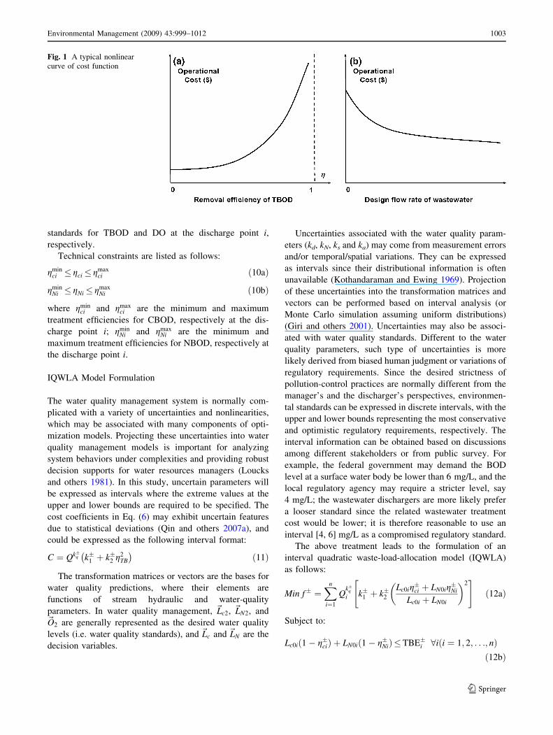
wastewater flow rate. Figure 1a shows a typical monoto-

nously increasing nonlinear curve of TBOD removal

efficiency vs. the operational cost for a wastewater treat-

ment plant while the wastewater flow rate keeps constant

(Cheng and Cheng 1990; Zeng and others 2003). The

nonlinearity reflects the economy-of-efficiency where the

treatment cost per unit of pollutant loading will increase

with the treatment efficiency. It is indicated that the non-

linear relationships could be approximated by a quadratic

function with a reasonable degree of error as C = a ? bg2,

where a and b are cost coefficients (Huang and others

1995). Figure 1b presents a typical curve of the operational

cost vs. the treatment scale while the TBOD removal rate

keeps constant; this reflects the economy-of-scale effects.

Therefore, a combined nonlinear cost function can be

expressed as follows (Cheng and Cheng 1990):

C ¼ Qkscale k1 þ k2g2TB

� �ð6Þ

where C is the operational cost for a wastewater treatment

plant, [$]; Q is the design flow rate of wastewater treatment

(treatment scale) [ML-3]; gTB is the removal efficiency of

TBOD; k1 and k2 are the cost-function coefficients (k1,

k2 [ 0); kscale is the economy-of-scale index ranging from

0.7 to 0.9 (Huang and others 1995). The parameters of

kscale, k1, k2 are obtained from statistical analysis and

normally vary with different type of wastewater that is to

be treated. Typical values can be found in Rinaldi and

others (1979), Cheng and Cheng (1990), Lee and Wen

(1997), and Qin and others (2007a).

Since TBOD is the sum of CBOD and NBOD, we can

use the following relationships to correlate gci and gNi with

the cost function (Ci):

Lc0i þ LN0i ¼ LTB0i ð7aÞLci þ LNi ¼ LTBi ð7bÞ

gci ¼Lci

Lc0i; gNi ¼

LNi

LN0i; gTBi ¼

LTBi

LB0ið7cÞ

gTBiLB0i ¼ gciLc0i þ gNiLN0i ð7cÞ

where Lc0i and LN0i are the initial concentrations of CBOD

and NBOD at discharge point i, [ML-3]; Lci and LNi are the

discharge concentrations of CBOD and NBOD at discharge

point i, [ML-3]; LTB0i and LTBi are initial and discharge

concentrations of TBOD at discharge point i, [ML-3]; gTBi

is the TBOD treatment efficiency at discharge point i.

Water Quality Constraints

Constraint equations associated with the TBOD effluent

standards at each discharge point are (Loucks and others

1981):

Lc0ið1� gciÞ þ LN0ið1� gNiÞ�TBEi 8i ð8Þ

where TBEi is the effluent discharge standard for the dis-

charge point i.

For any water quality segment in the waste-receiving

water body, the stream quality standards for TBOD and DO

concentrations can be expressed as follows (Loucks and

others 1981):

Xn

i¼1

UcjiLc0ið1� gciÞ� �

þ mcj

þXn

i¼1

UNjiLN0ið1� gNiÞ� �

þ mNj�TBWj 8j ð9aÞ

Xn

i¼1

VcjiLc0ið1� gciÞ� �

þXn

i¼1

VNjiLN0ið1� gNiÞ� �

þ nj�DOWj 8j ð9bÞ

where Ucji, UNji, Vcji, and VNji are the elements at the jth

row and the ith column (j = 1, 2, …, n; i = 1, 2, …, n) of

the transformation matrices (Uc, UN, Vc, and VN), respec-

tively; j denotes the index of river segment; mcj, mNj, and nj

are the element at the jth row of transformation vectors (m~c,

m~N , and n~); TBWj and DOWj are the stream water quality

1002 Environmental Management (2009) 43:999–1012

123

standards for TBOD and DO at the discharge point i,

respectively.

Technical constraints are listed as follows:

gminci � gci� gmax

ci ð10aÞ

gminNi � gNi� gmax

Ni ð10bÞ

where gminci and gmax

ci are the minimum and maximum

treatment efficiencies for CBOD, respectively at the dis-

charge point i; gminNi and gmax

Ni are the minimum and

maximum treatment efficiencies for NBOD, respectively at

the discharge point i.

IQWLA Model Formulation

The water quality management system is normally com-

plicated with a variety of uncertainties and nonlinearities,

which may be associated with many components of opti-

mization models. Projecting these uncertainties into water

quality management models is important for analyzing

system behaviors under complexities and providing robust

decision supports for water resources managers (Loucks

and others 1981). In this study, uncertain parameters will

be expressed as intervals where the extreme values at the

upper and lower bounds are required to be specified. The

cost coefficients in Eq. (6) may exhibit uncertain features

due to statistical deviations (Qin and others 2007a), and

could be expressed as the following interval format:

C ¼ Qk�q k�1 þ k�2 g2TB

� �ð11Þ

The transformation matrices or vectors are the bases for

water quality predictions, where their elements are

functions of stream hydraulic and water-quality

parameters. In water quality management, L~c2, L~N2, and

O~2 are generally represented as the desired water quality

levels (i.e. water quality standards), and L~c and L~N are the

decision variables.

Uncertainties associated with the water quality param-

eters (kd, kN, ks and ka) may come from measurement errors

and/or temporal/spatial variations. They can be expressed

as intervals since their distributional information is often

unavailable (Kothandaraman and Ewing 1969). Projection

of these uncertainties into the transformation matrices and

vectors can be performed based on interval analysis (or

Monte Carlo simulation assuming uniform distributions)

(Giri and others 2001). Uncertainties may also be associ-

ated with water quality standards. Different to the water

quality parameters, such type of uncertainties is more

likely derived from biased human judgment or variations of

regulatory requirements. Since the desired strictness of

pollution-control practices are normally different from the

manager’s and the discharger’s perspectives, environmen-

tal standards can be expressed in discrete intervals, with the

upper and lower bounds representing the most conservative

and optimistic regulatory requirements, respectively. The

interval information can be obtained based on discussions

among different stakeholders or from public survey. For

example, the federal government may demand the BOD

level at a surface water body be lower than 6 mg/L, and the

local regulatory agency may require a stricter level, say

4 mg/L; the wastewater dischargers are more likely prefer

a looser standard since the related wastewater treatment

cost would be lower; it is therefore reasonable to use an

interval [4, 6] mg/L as a compromised regulatory standard.

The above treatment leads to the formulation of an

interval quadratic waste-load-allocation model (IQWLA)

as follows:

Min f� ¼Xn

i¼1

Qk�qi k�1 þ k�2

Lc0ig�ci þ LN0ig�Ni

Lc0i þ LN0i

� �2" #

ð12aÞ

Subject to:

Lc0ið1� g�ciÞ þ LN0ið1� g�NiÞ�TBE�i 8iði ¼ 1; 2; . . .; nÞð12bÞ

Fig. 1 A typical nonlinear

curve of cost function

Environmental Management (2009) 43:999–1012 1003

123

Xn

i¼1

U�cijLc0ið1� g�ciÞh i

þ m�cj

þXn

i¼1

U�NjiLN0ið1� g�NiÞh i

þ m�Nj�TBW�j 8jðj

¼ 1; 2; . . .; nÞ ð12cÞXn

i¼1

V�cjiLc0ið1� g�ciÞh i

þXn

i¼1

V�NjiLN0ið1� g�NiÞh i

þ n�j �DOW�j 8jðj

¼ 1; 2; . . .; nÞ ð12dÞ

gminci � g�ci � gmax

ci ð12eÞ

gminNi � g�Ni� gmax

Ni ð12fÞ

Due to the existence of the cross-product terms of gci

and gNi in the cost function (12a), the formulated IQWLA

model is difficult to solve. A dual response regression

technique can be used to transform it to a pure quadratic

form. Detailed procedures can be found in Kennedy and

Gentle (1981) and Kim and Lin (1998). Then, model (12)

turns into a typical inexact quadratic program (IQP) and

can be solved by algorithms proposed by Huang and others

(1995) and Chen and Huang (2001). The constraints (12e)

and (12f) are technical constraints and will be restricted by

the capacities of the currently available treatment

technologies. The constraints may be redundant when the

capacity of wastewater treatment is not a major concern. In

such a case, gminNi and gmax

Ni could be 0 and 1, respectively. In

addition, several conditions need to be satisfied to ensure

existence of optimal solution for a QP problem. When the

objective function to a QP problem is strictly convex for all

feasible points the problem has a unique local minimum

which is also the global minimum (Qin and others 2007c,

2008c). A sufficient condition to guarantee strictly

convexity is for the coefficients of quadratic terms to be

positive definite (Huang and others 1995). As the function

describing operating cost of water treatment is generally

monotone increasing, the objective function (12a) is

concave. This ensures an optimal solution for the model.

Case Study

Background

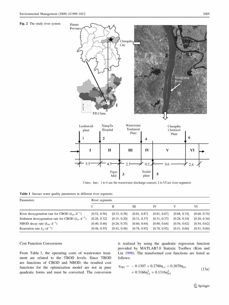
The Xiangjiang River section (from Houzishi to Chen-

guanzhen areas) flowing through the City of Changsha,

Hunan Province, China, will be provided as a case to dem-

onstrate the applicability of the proposed methodology. This

river section, with a length of about 25 km, receives the

majority of wastewater discharged from the City of Chang-

sha. Six main discharging sources exist along the section,

including the Changsha Leatheroid Plant, the Xiangya Hos-

pital, the Hunan Paper Mill, the No. 1 Wastewater Treatment

Plant, the Changsha Textile Plant and the Changsha Chemical

Plant (Qin and others 2007a). In order to meet the environ-

mental requirement, the raw wastewater from each industry

must be treated with specific facilities before discharge. The

operating costs of these facilities were directly related to the

inflow of wastewater and the level of its treatment. The water

quality in the river was related to contaminant concentrations

and flow rate of the discharged wastewater. It is desired that a

waste-load-allocation model be developed in order to mini-

mize the operating cost and satisfy the national

environmental standard, through identification of desired

wastewater treatment efficiencies (or allowable discharge

amounts) for the six discharging sources.

Details of the related water-quality parameters were

provided in Zeng and others (2004). Figure 2 is a sche-

matic diagram of the study system. Table 1 shows water

quality data in different river segments. Uncertainties

associated with BOD deoxygenation and decay rates (kdi,

kNi and ksi) and reaeration rate (kai) due to dynamic and

fluctuating features were handled as intervals. Table 2

presents the wastewater discharge data from various sour-

ces. The cost function of each discharge source is listed in

Table 3. These functions were derived from the data as

reported in Qin and Zeng (2002) and Zeng and others

(2004). The coefficients of these functions are expressed as

intervals due to the uncertainties in the obtained informa-

tion, including parameters kq, k1 and k2.

The right-hand sides of optimization-model constraints

(e.g. water quality standards) are also expressed as intervals.

Table 4 shows the national surface-water standards for

TBOD and DO and the national wastewater-discharge

standards of TBOD for industrial sectors (SEPA 1996,

2002). According to Table 4, the intervals of allowable

TBOD and DO levels in the river system are identified as [4,

6] and [3, 5] mg/L, respectively. The allowable interval for

BOD concentrations in the leatheroid plant, paper mill and

textile plant are determined as [150, 600] mg/L. Those for

chemical and hospital wastewater, the intervals are [60, 300]

mg/L. Since there is no Class III standard available for

wastewater treatment plant, we assume it is 60 mg/L; then,

the corresponding interval becomes [30, 60] mg/L. Due to

capacity restrictions of available wastewater treatment

technologies, we assume the maximum possible treatment

efficiencies for both CBOD and NBOD are 95%. The river

water level has large variations during different seasons, with

a maximum level at 39 m (1998) and minimum one at 25 m

(1999). The study period is assumed at the drought season

when the point-source pollution problem is most serious. The

width of the river system is ranging from 400 to 1000 m and

the ratio of the river width to length is negligible, such that

the river system will be considered as one-dimensional.

1004 Environmental Management (2009) 43:999–1012

123

Cost Function Conversions

From Table 3, the operating costs of wastewater treat-

ment are related to the TBOD levels. Since TBOD

are functions of CBOD and NBOD, the resulted cost

functions for the optimization model are not in pure

quadratic forms and must be converted. The conversion

is realized by using the quadratic regression function

provided by MATLAB7.0 Statistic Toolbox (Kim and

Lin 1998). The transformed cost functions are listed as

follows:

gTB1 ¼ � 0:1307þ 0:2780gc1 þ 0:2670gN1

þ 0:3166g2c1 þ 0:1316g2

N1

ð13aÞ

Fig. 2 The study river system

Table 1 Inexact water quality parameters in different river segments

Parameters River segments

I II III IV V VI

River deoxygenation rate for CBOD (kdi, d-1) [0.52, 0.56] [0.33, 0.38] [0.81, 0.87] [0.81, 0.87] [0.68, 0.74] [0.68, 0.74]

Sediment deoxygenation rate for CBOD (ksi, d-1) [0.28, 0.32] [0.15, 0.20] [0.31, 0.37] [0.31, 0.37] [0.28, 0.34] [0.28, 0.34]

NBOD decay rate (kNi, d-1) [0.40, 0.46] [0.26, 0.35] [0.60, 0.64] [0.60, 0.64] [0.54, 0.62] [0.54, 0.62]

Reaeration rate kai (d-1) [0.48, 0.55] [0.42, 0.48] [0.78, 0.92] [0.78, 0.92] [0.51, 0.60] [0.51, 0.60]

Environmental Management (2009) 43:999–1012 1005

123

gTB2 ¼� 0:1077þ 0:2195gc2 þ 0:1991gN2

þ 0:3370g2c2 þ 0:2414g2

N2

ð13bÞ

gTB3 ¼� 0:1234þ 0:2328gc3 þ 0:2618gN3

þ 0:1888g2c3 þ 0:3178g2

N3

ð13cÞ

gTB4 ¼� 0:1075þ 0:2026gc4 þ 0:2262gN4 þ 0:1566g2c4

þ 0:4122g2N4 ð13dÞ

gTB5 ¼ �0:1168þ 0:2248gc5 þ 0:2219gN5 þ 0:3979g2c5

þ 0:1647g2N5

gTB6 ¼� 0:1213þ 0:2145gc6 þ 0:2719gN6 þ 0:2055g2c6

þ 0:3063g2N6 ð13eÞ

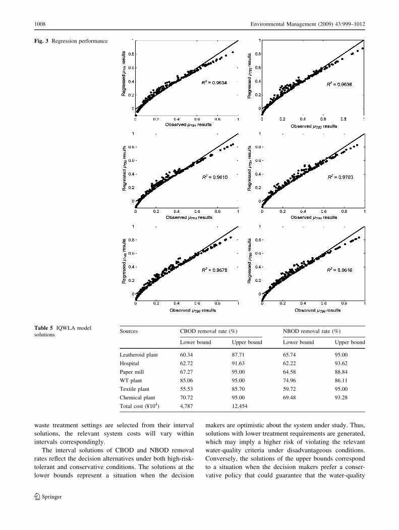
A standard R-square test is performed using 200

randomly generated samples of gc1 and gN1. Figure 3

shows the detailed regression performance, where the

observed results denote the calculated gTBi using

equations provided in Table 3, and the regression results

denote those from using the converted pure quadratic

equations. It is found that most of the R-square levels are

higher than 0.96. The R-square level is calculated by the

following equation:

R2 ¼½Pns

i¼1 ðypi � �ypÞðyoi � �yoÞ�2Pns

i¼1 ðypi � �ypÞ2Pns

i¼1 ðyoi � �yoÞ2ð14Þ

where yoi denotes observed data; ypi means regressed data;

�yo is mean value of yo; �yp is mean value of yp; ns is number

of samples. The results imply that these functions can

reasonably approximate values of gTBi (i = 1, 2, …, 6).

Formulation of IQWLA Model

Based on water quality simulation models with interval

analysis, the interval-parameter transformation matrices

U�c ;U�N ;V

�c and V�N

� �and vectors m~�c ;m~

�N and n~�

� �are

obtained as follows:

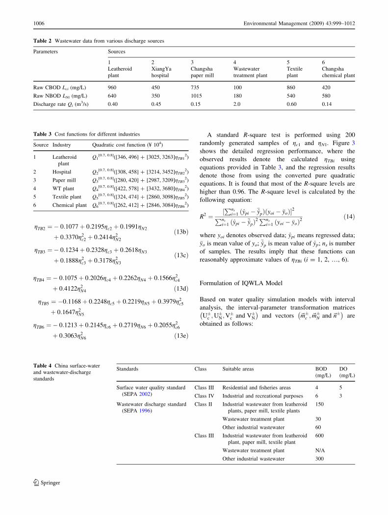
Table 2 Wastewater data from various discharge sources

Parameters Sources

1 2 3 4 5 6

Leatheroid

plant

XiangYa

hospital

Changsha

paper mill

Wastewater

treatment plant

Textile

plant

Changsha

chemical plant

Raw CBOD Lci (mg/L) 960 450 735 100 860 420

Raw NBOD LNi (mg/L) 640 350 1015 180 540 580

Discharge rate Qi (m3/s) 0.40 0.45 0.15 2.0 0.60 0.14

Table 3 Cost functions for different industries

Source Industry Quadratic cost function (¥ 104)

1 Leatheroid

plant

Q1[0.7, 0.8]([346, 496] ? [3025, 3263]gTB1

2)

2 Hospital Q2[0.7, 0.8]([308, 458] ? [3214, 3452]gTB2

2)

3 Paper mill Q3[0.7, 0.8]([280, 420] ? [2987, 3209]gTB3

2)

4 WT plant Q4[0.7, 0.8]([422, 578] ? [3432, 3680]gTB4

2)

5 Textile plant Q5[0.7, 0.8]([324, 474] ? [2860, 3098]gTB5

2)

6 Chemical plant Q6[0.7, 0.8]([262, 412] ? [2846, 3084]gTB6

2)

Table 4 China surface-water

and wastewater-discharge

standards

Standards Class Suitable areas BOD

(mg/L)

DO

(mg/L)

Surface water quality standard

(SEPA 2002)

Class III Residential and fisheries areas 4 5

Class IV Industrial and recreational purposes 6 3

Wastewater discharge standard

(SEPA 1996)

Class II Industrial wastewater from leatheroid

plants, paper mill, textile plants

150

Wastewater treatment plant 30

Other industrial wastewater 60

Class III Industrial wastewater from leatheroid

plant, paper mill, textile plant

600

Wastewater treatment plant N/A

Other industrial wastewater 300

1006 Environmental Management (2009) 43:999–1012

123

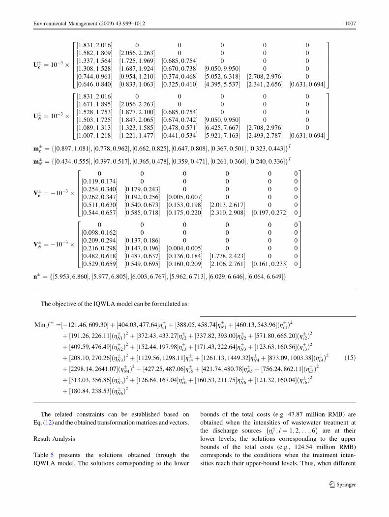
The objective of the IQWLA model can be formulated as:

The related constraints can be established based on

Eq. (12) and the obtained transformation matrices and vectors.

Result Analysis

Table 5 presents the solutions obtained through the

IQWLA model. The solutions corresponding to the lower

bounds of the total costs (e.g. 47.87 million RMB) are

obtained when the intensities of wastewater treatment at

the discharge sources g�i ; i ¼ 1; 2; . . .; 6� �

are at their

lower levels; the solutions corresponding to the upper

bounds of the total costs (e.g., 124.54 million RMB)

corresponds to the conditions when the treatment inten-

sities reach their upper-bound levels. Thus, when different

U�c ¼ 10�3 �

½1:831; 2:016� 0 0 0 0 0

½1:582; 1:809� ½2:056; 2:263� 0 0 0 0

½1:337; 1:564� ½1:725; 1:969� ½0:685; 0:754� 0 0 0

½1:308; 1:528� ½1:687; 1:924� ½0:670; 0:738� ½9:050; 9:950� 0 0

½0:744; 0:961� ½0:954; 1:210� ½0:374; 0:468� ½5:052; 6:318� ½2:708; 2:976� 0

½0:646; 0:840� ½0:833; 1:063� ½0:325; 0:410� ½4:395; 5:537� ½2:341; 2:656� ½0:631; 0:694�

26666664

37777775

U�N ¼ 10�3 �

½1:831; 2:016� 0 0 0 0 0

½1:671; 1:895� ½2:056; 2:263� 0 0 0 0

½1:528; 1:753� ½1:877; 2:100� ½0:685; 0:754� 0 0 0

½1:503; 1:725� ½1:847; 2:065� ½0:674; 0:742� ½9:050; 9:950� 0 0

½1:089; 1:313� ½1:323; 1:585� ½0:478; 0:571� ½6:425; 7:667� ½2:708; 2:976� 0

½1:007; 1:218� ½1:221; 1:477� ½0:441; 0:534� ½5:921; 7:163� ½2:493; 2:787� ½0:631; 0:694�

26666664

37777775

m�c ¼ f½0:897; 1:081�; ½0:778; 0:962�; ½0:662; 0:825�; ½0:647; 0:808�; ½0:367; 0:501�; ½0:323; 0:443�gT

m�N ¼ f½0:434; 0:555�; ½0:397; 0:517�; ½0:365; 0:478�; ½0:359; 0:471�; ½0:261; 0:360�; ½0:240; 0:336�gT

V�c ¼ �10�3 �

0 0 0 0 0 0

½0:119; 0:174� 0 0 0 0 0

½0:254; 0:340� ½0:179; 0:243� 0 0 0 0

½0:262; 0:347� ½0:192; 0:256� ½0:005; 0:007� 0 0 0

½0:511; 0:630� ½0:540; 0:673� ½0:153; 0:198� ½2:013; 2:617� 0 0

½0:544; 0:657� ½0:585; 0:718� ½0:175; 0:220� ½2:310; 2:908� ½0:197; 0:272� 0

26666664

37777775

V�N ¼ �10�3 �

0 0 0 0 0 0

½0:098; 0:162� 0 0 0 0 0

½0:209; 0:294� ½0:137; 0:186� 0 0 0 0

½0:216; 0:298� ½0:147; 0:196� ½0:004; 0:005� 0 0 0

½0:482; 0:618� ½0:487; 0:637� ½0:136; 0:184� ½1:778; 2:423� 0 0

½0:529; 0:659� ½0:549; 0:695� ½0:160; 0:209� ½2:106; 2:761� ½0:161; 0:233� 0

26666664

37777775

n� ¼ f½5:953; 6:860�; ½5:977; 6:805�; ½6:003; 6:767�; ½5:962; 6:713�; ½6:029; 6:646�; ½6:064; 6:649�g

Min f� ¼ �121:46; 609:30½ � þ 404:03; 477:64½ �g�c1 þ 388:05; 458:74½ �g�N1 þ 460:13; 543:96½ �ðg�c1Þ2

þ 191:26; 226:11½ �ðg�N1Þ2 þ 372:43; 433:27½ �g�c2 þ 337:82; 393:00½ �g�N2 þ 571:80; 665:20½ �ðg�c2Þ

2

þ 409:59; 476:49½ �ðg�N2Þ2 þ 152:44; 197:98½ �g�c3 þ 171:43; 222:64½ �g�N3 þ 123:63; 160:56½ �ðg�c3Þ

2

þ 208:10; 270:26½ �ðg�N3Þ2 þ 1129:56; 1298:11½ �g�c4 þ 1261:13; 1449:32½ �g�N4 þ 873:09; 1003:38½ �ðg�c4Þ

2

þ 2298:14; 2641:07½ �ðg�N4Þ2 þ 427:25; 487:06½ �g�c5 þ 421:74; 480:78½ �g�N5 þ 756:24; 862:11½ �ðg�c5Þ

2

þ 313:03; 356:86½ �ðg�N5Þ2 þ 126:64; 167:04½ �g�c6 þ 160:53; 211:75½ �g�N6 þ 121:32; 160:04½ �ðg�c6Þ

2

þ 180:84; 238:53½ �ðg�N6Þ2

ð15Þ

Environmental Management (2009) 43:999–1012 1007

123

waste treatment settings are selected from their interval

solutions, the relevant system costs will vary within

intervals correspondingly.

The interval solutions of CBOD and NBOD removal

rates reflect the decision alternatives under both high-risk-

tolerant and conservative conditions. The solutions at the

lower bounds represent a situation when the decision

makers are optimistic about the system under study. Thus,

solutions with lower treatment requirements are generated,

which may imply a higher risk of violating the relevant

water-quality criteria under disadvantageous conditions.

Conversely, the solutions of the upper bounds correspond

to a situation when the decision makers prefer a conser-

vative policy that could guarantee that the water-quality

Fig. 3 Regression performance

Table 5 IQWLA model

solutionsSources CBOD removal rate (%) NBOD removal rate (%)

Lower bound Upper bound Lower bound Upper bound

Leatheroid plant 60.34 87.71 65.74 95.00

Hospital 62.72 91.63 62.22 93.62

Paper mill 67.27 95.00 64.58 88.84

WT plant 85.06 95.00 74.96 86.11

Textile plant 55.53 85.70 59.72 95.00

Chemical plant 70.72 95.00 69.48 93.28

Total cost (¥104) 4,787 12,454

1008 Environmental Management (2009) 43:999–1012

123

criteria be met. In such a case, higher treatment require-

ments are desired. The obtained interval solutions can help

decision makers analyze the tradeoffs between system cost

and potential risk. Generally, a post-modeling analysis

based on public survey, round-table discussion, and expert

consultation would be necessary to help reach a final

decision.

For example, when the decision makers aim toward a

lower system cost, only primary treatment (i.e., 55.53%

and 59.72% for CBOD and NBOD) would be needed for

the textile plant; when the decision makers aim towards a

lower risk of water quality standard violation (a higher

system cost), tertiary treatment facilities would have to be

used in order to reach high pollutant-removal efficiencies

(i.e., 85.70% and 95.00% for CBOD and NBOD, respec-

tively). Except for the wastewater treatment plant, a

secondary treatment would be sufficient for most of the

discharge sources under an optimistic consideration.

However, when environmental protection is of severe

concern by local government, all discharge sources would

require tertiary treatment.

The result in Table 5 indicates that different treatment

intensities are allocated to the discharge sources in order to

obtain a minimum system cost. It appears that the required

CBOD and NBOD treatment (i.e. [85.06, 95.00] and

[74.96, 86.11]%, respectively) for the wastewater treatment

plant are the most stringent, followed by the chemical

plant, paper mill, and leatheroid plant. This is due to the

fact that the TBOD discharge standard for wastewater

treatment plant (i.e. [30, 60] mg/L) is strictest among all

discharge sources. The high treatment requirement for

chemical plant may due to its relatively stricter discharge

criteria and low unit treatment cost (see Table 3). The

relatively higher treatment requirements for the leatheroid

plant and paper mill may be the result of their higher

CBOD and NBOD levels in raw wastewater.

The above results demonstrate that the optimization

model can effectively communicate the interval-format

uncertainties into the optimization process, and generate

inexact solutions that contain a spectrum of potential

wastewater treatment options. The decision alternatives can

be obtained by adjusting different combinations of the

decision variables within their solution intervals. The results

are valuable for supporting local decision makers in gener-

ating cost-effective water quality management schemes.

The interval solutions of the IQWLA model contain a

full spectrum of possible decision variables under uncer-

tainty, leading to a wide decision spaces for decision

makers. The right-hand sides of the constraints are envi-

ronmental guidelines, where the associated uncertainties

could be derived from human judgment or variations of

regulatory requirements. Through round-table discussion

among various stakeholders, the uncertainty can be

effectively reduced, and the wideness of the regulatory

intervals can be properly controlled. For example, if a

stricter pollution control strategy is preferred (i.e. strict

scenario), the allowable TBOD and DO intervals of surface

water quality can be decided as [4, 5] and [4, 5] mg/L,

respectively; they belong to the stricter half parts of the

intervals [4, 6] and [3, 5] mg/L. Similarly, the less strict half

parts of intervals can be determined as [5, 6] and [3, 4] mg/

L, respectively. This corresponds to a loose scenario. A

similar treatment can be performed to the wastewater dis-

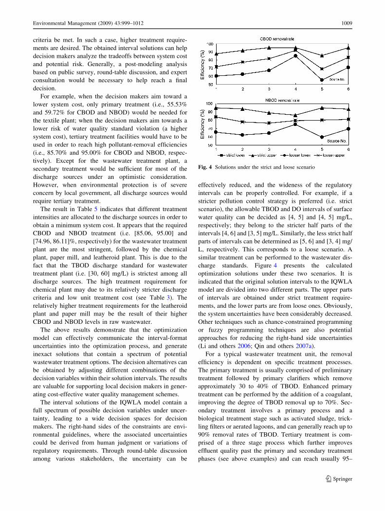
charge standards. Figure 4 presents the calculated

optimization solutions under these two scenarios. It is

indicated that the original solution intervals to the IQWLA

model are divided into two different parts. The upper parts

of intervals are obtained under strict treatment require-

ments, and the lower parts are from loose ones. Obviously,

the system uncertainties have been considerably decreased.

Other techniques such as chance-constrained programming

or fuzzy programming techniques are also potential

approaches for reducing the right-hand side uncertainties

(Li and others 2006; Qin and others 2007a).

For a typical wastewater treatment unit, the removal

efficiency is dependent on specific treatment processes.

The primary treatment is usually comprised of preliminary

treatment followed by primary clarifiers which remove

approximately 30 to 40% of TBOD. Enhanced primary

treatment can be performed by the addition of a coagulant,

improving the degree of TBOD removal up to 70%. Sec-

ondary treatment involves a primary process and a

biological treatment stage such as activated sludge, trick-

ling filters or aerated lagoons, and can generally reach up to

90% removal rates of TBOD. Tertiary treatment is com-

prised of a three stage process which further improves

effluent quality past the primary and secondary treatment

phases (see above examples) and can reach usually 95–

Fig. 4 Solutions under the strict and loose scenario

Environmental Management (2009) 43:999–1012 1009

123

98% removal rates of TBOD. The solution from the opti-

mization model represents a group of theoretically ideal

removal rates for TBOD (including both CBOD and

NBOD) at various discharge points. In practical applica-

tions, it is normally difficult to accurately control the

treatment efficiency at a specific level. In many cases,

combinations of different treatment processes could be

used to meet the required standards, since each type of

treatment has a certain treatment efficiency range for dif-

ferent quality parameters. For example, the treatment

processes for the six discharging industries under the most

conservative conditions (corresponding to the upper

bounds of the solutions as shown in Table 5) could be

secondary, tertiary, secondary, secondary, secondary and

tertiary, respectively; under the most optimistic conditions,

the treatment processes could be enhanced primary,

enhanced primary, enhanced primary, secondary, enhanced

primary, and secondary, respectively.

Generally, the solutions from the IQWLA model

demonstrate tradeoffs between the overall wastewater

treatment cost and the system-failure risk due to inherent

uncertainties that exist in various system components.

Planning with a higher system cost may guarantee that the

water-quality management requirements and environmen-

tal regulations be met (i.e., higher system reliability); if

the plan aims towards a lower system cost, the possibility

of meeting the requirements by the suggested treatment

requirements decreases (i.e., higher system risk). In

practical applications, the allowable levels of environ-

mental violations could be decided based on discussions

among stakeholders, and the decision variables could be

adjusted continuously within their solution intervals

according to specific system conditions. This would allow

decision makers to incorporate more implicit knowledge

(such as socio-economic conditions), if required for the

decision.

Conclusions

A simulation-based interval quadratic waste load allocation

(IQWLA) model was developed in this study for river water

quality management. Uncertainties associated with water

quality parameters, cost functions, and environmental

guidelines were reflected as interval parameters. The cost

functions of wastewater treatment plant were expressed as

quadratic forms. A water quality planning problem in the

Changsha section of the Xiangjiang River in China was

used as a study case to demonstrate the applicability of the

proposed method. The study results demonstrated that the

proposed simulation-based IQWLA model could effec-

tively communicate the interval-format uncertainties into

the optimization process, and generate inexact solutions that

contain a spectrum of potential wastewater treatment

options. Decision alternatives can be obtained by adjusting

different combinations of the decision variables within their

solution intervals. The results are valuable for supporting

local decision makers in generating cost-effective water

quality management schemes.

The research work was advantageous over the previous

studies in the following aspects: (i) a multi-segment water

quality model was developed to generate water-quality

transformation matrices and vectors, which could be

embedded directly into a water quality management model;

(ii) uncertainties associated with water quality parameters

could be projected to optimization models through interval

analysis; (iii) the nonlinearity problem associated with the

objective function of wastewater treatment could be miti-

gated by quadratic regression technique.

The water simulation system proposed in this study is

suitable for one-dimensional steady-state river systems, with

CBOD, NBOD and DO levels being the main water-quality

indicators. In further studies, additional water-quality indi-

cators such as chemical oxygen demand (COD) and

phosphates can also be handled through developing similar

transformation matrices/vectors. In practical applications,

the solutions from the proposed water quality management

model are suitable for a preliminary evaluation of various

alternatives and for identifying the important data require-

ment before initiation of more extensive or expensive data

collection and simulation studies. The model solution would

be more applicable, if post-modeling analyses such as multi-

criteria decision analysis, group decision making, and public

survey can be performed.

Acknowledgments This research was supported by the Major State

Basic Research Development Program of MOST (2005CB724200 and

2006CB403307), the Canadian Water Network under the Networks of

Centers of Excellence (NCE), and the Natural Science and Engi-

neering Research Council of Canada. The authors deeply appreciate

the editor and the anonymous reviewers for their insightful comments

and suggestions.

References

Bouwer H (2003) Integrated water management for the 21st century:

problems and solutions. Food Agriculture and Environment

1:118–127

Burn DH, McBean EA (1987) Application of nonlinear optimization

to water quality. Applied Mathematical Modelling 11:438–446

Chen MJ, Huang GH (2001) A derivative algorithm for inexact

quadratic program–application to environmental decision-mak-

ing under uncertainty. European Journal of Operational Research

128:570–586

Cheng ST, Cheng LL (1990) Environmental systems analysis. China

Higher Education Press, Beijing

Dupacova J, Gaivoronski A, Kos Z, Szantai T (1991) Stochastic

programming in water management: a case study and a

comparison of solution techniques. European Journal of Oper-

ational Research 52:28–44

1010 Environmental Management (2009) 43:999–1012

123

Fu GW, Cheng ST (1985) Systems planning for water pollution

control. Tsinghua University Press, Beijing

Fujiwara O (1988) River basin water quality management in

stochastic environment. Journal of Environmental Engineering

114:864–877

Gen M, Ida K, Lee J (1997) Fuzzy nonlinear goal programming

using genetic algorithm. Computers and Industrial Engineering

33:39–42

Giri BS, Karimi IA, Ray MB (2001) Modeling and Monte Carlo

simulation of TCDD transport in a river. Water Research

35:1263–1279

Huang GH (1998) A hybrid inexact-stochastic water management

model. European Journal of Operational Research 107:137–158

Huang GH, Chang NB (2003) The perspectives of environmental

informatics and systems analysis. Journal of Environmental

Informatics 191:1–6

Huang GH, Loucks DP (2000) An inexact two-stage stochastic

programming model for water resources management under

uncertainty. Civil Engineering and Environmental Systems

17:95–118

Huang GH, Qin XS (2008a) Environmental systems analysis under

uncertainty. Civil Engineering and Environmental Systems

25:77–80

Huang GH, Qin XS (2008b) Editorial: climate change and sustainable

energy development. Energy Sources, Part A – Recovery

Utilization and Environmental Effects 30:1281–1285

Huang GH, Baetz BW, Patry GG (1992) An interval linear

programming approach for municipal solid waste management

planning under uncertainty. Civil Engineering Systems 9:

319–335

Huang GH, Baetz BW, Party GG (1995) Grey quadratic programming

and its application to municipal solid waste management

planning under uncertainty. Engineering Optimization 23:

201–223

Huang YF, Huang GH, Baetz BW, Liu L (2002) Violation analysis

for solid waste management systems: an interval fuzzy pro-

gramming approach. Journal of Environmental Management

65:431–446

Karmakar S, Mujumdar PP (2006) Grey fuzzy optimization model for

water quality management of a river system. Advances in Water

Resources 29:1088–1105

Kennedy WJ, Gentle JE (1981) Statistics: textbooks and monographs.

Marcel Dekker, New York, pp 200–270

Kim KJ, Lin DKJ (1998) Dual response surface optimization: a fuzzy

modeling approach. Journal of Quality Technology 30:1–10

Kothandaraman V, Ewing BB (1969) A probabilistic analysis of

dissolved oxygen-biochemical oxygen demand relationship in

streams. Journal of Water Pollution Control Federation 41:

155–162

Lee CS, Chang SP (2005) Interactive fuzzy optimization for an

economic and environmental balance in a river system. Water

Research 39:221–231

Lee CS, Wen CG (1996) River assimilative capacity analysis

via fuzzy linear programming. Fuzzy Sets and Systems 79:

191–201

Lee CS, Wen CG (1997) Fuzzy goal programming approach for water

quality management in a river basin. Fuzzy Sets and Systems

89:181–192

Li YP, Huang GH, Baetz BW (2006) Environmental management

under uncertainty—an internal-parameter two-stage chance-

constrained mixed integer linear programming method. Envi-

ronmental Engineering Science 23:761–779

Liu Y, Guo HC, Zhang ZX, Wang LJ, Dai YL, Fan YY (2007) An

optimization method based on scenario analyses for watershed

management under uncertainty. Environmental Management

39(5):678–690

Liu Y, Yang PJ, Hu C, Guo HC (2008) Water quality modeling for

load reduction under uncertainty: a Bayesian approach. Water

Research, doi:10.1016/j.watres.2008.04.007

Loucks DP (2003) Managing America’s rivers: who’s doing it?

International Journal of River Basin Management 1:21–31

Loucks DP, Stedinger JR, Haith DA (1981) Water resource systems

planning and analysis. Prentice-Hall Inc., Englewood Cliffs,

New Jersey

Loucks DP, Kindler J, Fedra K (1985) Interactive water resources

modeling and model use: an overview. Water Resources

Research 21:95–102

Marr JK, Canale RP (1988) Load allocation for toxics using Monte

Carlo techniques, Journal—Water Pollution Control Federation

60:659–666

Mujumdar PP, Sasikumar K (2002) A fuzzy risk approach for

seasonal water quality management of a river system. Water

Resources Research 38: doi:10.1029/2000WR000126

Mujumdar PP, Saxena P (2004) A stochastic dynamic programming

model for stream water quality management. Sadhana 29:477–

497

O’Connor DJ, Dobbins WE (1958) Mechanisms of reaeration in

natural streams. Transactions of the American Society of Civil

Engineering 123:641–684

Qin XS, Zeng GM (2002) Application of genetic algorithm to gray

non-linear programming problems for water environment.

Advances in Water Science (China) 13:32–37

Qin XS, Huang GH, Zeng GM, Chakma A, Huang YF (2007a) An

interval-parameter fuzzy nonlinear optimization model for

stream water quality management under uncertainty. European

Journal of Operational Research 180:1331–1357

Qin XS, Huang GH, Zeng GM, Chakma A, Xi BD (2007b) A fuzzy

composting process model. Journal of Air & Waste Management

Association 57:535–550

Qin XS, Huang GH, Chakma A (2007c) A stepwise-inference-

based optimization system for supporting remediation of

petroleum-contaminated sites. Water, Air and Soil Pollution

185:349–368

Qin XS, Huang GH, Sun W, Chakma A (2008a) Optimizing

remediation operations at petroleum contaminated sites through

a simulation-based stochastic-MCDA approach. Energy Sources,

Part A – Recovery Utilization and Environmental Effects

30:1300–1326

Qin XS, Huang GH, Li YP (2008b) Risk management of BTEX

contamination in ground water – An integrtated fuzzy approach.

Ground Water 46:755–767

Qin XS, Huang GH, Zeng GM, Chakma A (2008c) Simulation-based

optimization of dual-phase vacuum extraction to remove non-

aqueous phase liquids in subsurface. Water Resources Research

44: W04422

Rauch W, Henze M, Koncsos L, Reichert P (1998) River water

quality modelling I. state of the art. In: Proceedings at the IAWQ

Biennial International Conference, Vancouver, British Colum-

bia, Canada, pp 21–26

Revelli R, Ridolfi L (2004) Stochastic dynamics of BOD in a

stream with random inputs. Advances in Water Resources 27:

943–952

Rinaldi S, Soncini-Sessa R, Stehfest H, Tamura H (1979) Modeling

and control of river quality. McGraw-Hill, New York, London

Sasikumar K, Mujumdar PP (1998) Fuzzy optimization model for

water quality management of river system. Journal of Water

Resources Planning and Management (ASCE) 124:79–84

SEPA (State Environmental Protection Administration) (1996) Indus-

trial wastewater discharge standard (GB8978–1996), Beijing

SEPA (State Environmental Protection Administration) (2002) Envi-

ronmental quality standard for surface water (GB3838–2002),

Beijing

Environmental Management (2009) 43:999–1012 1011

123

Thomann RV, Mueller JA (1987) Principles of surface water quality

modeling and control. Harper & Row, New York

Wu XY, Huang GH, Liu L, Li JB (2006) An interval nonlinear

program for the planning of waste management systems with

economies-of-scale effects—a case study for the region of

Hamilton, Ontario, Canada. European Journal of Operational

Research 171:349–372

Zeng GM, Lin YP, Qin XS, Huang GH, Li JB (2004) Optimum

municipal wastewater treatment plan design with consideration

of uncertainty. Journal of Environmental Sciences 16:126–131

Zeng GM, Qin XS, Wang W, Huang GH, Li JB, Statzner B (2003). Water

environmental planning considering the influence of non-linear

characteristics. Journal of Environmental Sciences 15:800–807

1012 Environmental Management (2009) 43:999–1012

123