Shorter time interval treatments for early medical abortions
Upload
khangminh22Category
view
0download
0
Estimation of the Early Post-Mortem Interval:
A Multicentre Comparison of the Analysis of Vitreous
Humour and the Henssge’s Nomogram Method.
A Cross-sectional, Correlational Study
Author: Lídia Giramé Rizzo
Clinical Tutor: Josep Ramis i Pujol
Methodological Tutor: Abel López Bermejo
IMLCF de Catalunya, Divisió de Girona
Facultat de Medicina, Universitat de Girona
November, 2019 – January, 2020

Acknowledgements
First of all, I would like to thank my clinical tutor, Josep Ramis i Pujol, for
dedicating part of his working time in sharing his knowledge, in keeping the project on
track from my first encounter to the final draft, for his patience and constant support.
My grateful thanks are also extended to all the team of forensic doctors of Institut de
Medicina Legal i Ciències Forenses de Catalunya Divisió de Girona for having welcomed me
so well and constantly making me feel as one of them.
I would like to express my greatest appreciation to various people for their
contribution to this project; Prof. Dr. Abel López Bermejo, for his periodic advice and
assistance; Prof. Dr. Marc Saez, for his valuable help in developing the statistical part of
this project; Dr. Bernardino González de la Presa and Mr. Vicente Guimerà Valverde
from Servei de Bioquímica de l’Hospital Clínic de Barcelona and Dr. Alba Anfruns Bagaria
from Serveis Tècnics de Recerca de la Universitat de Girona, for providing technical
information regarding the analysis of vitreous humour.
I would also like to extend my thanks to Dr. José Ignacio Muñoz Barús from
Instituto de Ciencias Forenses and Universidad de Santiago de Compostela, and Brita Zilg
from Department of Forensic Medicine and Karolinska Institutet of Stockholm, for providing
valuable information regarding their respective scientific papers.
Finally, I wish to thank my parents for their constant support and encouragement
throughout those three months of intense work and, in particular, my brother and
sister who contributed in giving me constructive feedback and useful advice in making
this project look better.
Thank you all.
Girona, 27 de gener de 2020.

Estimation of the Early Post-Mortem Interval:
A Multicentre Comparison of the Analysis of Vitreous Humour and the Henssge’s Nomogram Method
INDEX
1. SYMBOLS AND ABBREVIATIONS.............................................................................................................4
2. ABSTRACT .................................................................................................................................................... 5
3. INTRODUCTION ............................................................................................................................................ 6
3.1. ESTIMATING THE PMI .......................................................................................................................... 6 3.2. PMI METHODS .................................................................................................................................... 7
3.3. ALGOR MORTIS .................................................................................................................................... 8 3.4. RECTAL TEMPERATURE IN ESTIMATING POST-MORTEM INTERVAL. THE HENSSGE’S NOMOGRAM
METHOD ...................................................................................................................................................... 10 3.5. TANATOCHEMISTRY: THE ANALYSIS OF VITREOUS HUMOUR ............................................................... 14
3.6. VITREOUS HUMOUR’S POTASSIUM CONCENTRATION IN ESTIMATING POST-MORTEM INTERVAL ......... 16
4. JUSTIFICATION .......................................................................................................................................... 18
5. HYPOTHESES ............................................................................................................................................. 19
6. OBJECTIVES .............................................................................................................................................. 20
7. METHODOLOGY .......................................................................................................................................... 21
7.1. STUDY DESIGN ................................................................................................................................... 21
7.2. STUDY POPULATION ........................................................................................................................... 21 7.3. SAMPLING ......................................................................................................................................... 21
7.4. VARIABLES ........................................................................................................................................ 22 7.5. PROCESS OF DATA COLLECTION ........................................................................................................ 24
8. STATISTICAL ANALYSES ......................................................................................................................... 26
8.1. DESCRIPTIVE ANALYSIS ..................................................................................................................... 26
8.2. BIVARIATE ANALYSIS ......................................................................................................................... 26 8.3. MULTIVARIATE ANALYSIS ................................................................................................................... 26
9. ETHICAL ASPECTS................................................................................................................................... 28
10. STUDY LIMITATIONS ................................................................................................................................. 29
11. WORK PLAN ............................................................................................................................................... 31
12. CHRONOGRAM ..........................................................................................................................................32
13. BUDGET .......................................................................................................................................................33
14. REFERENCES ........................................................................................................................................... 35
15. ANNEXES ................................................................................................................................................... 40
15.1. PMI METHODS ................................................................................................................................. 40
15.2. HENSSGE’S NOMOGRAM ................................................................................................................... 42 15.3. PMI FORMULAS ............................................................................................................................... 44
15.4. LYTE INTEGRATED MULTI-SENSOR DATASHEET .............................................................................. 46 15.5. DIGITAL THERMOMETER WITH PROBE SENSOR TP3001 DATASHEET................................................ 47
15.6. COLORED WEATHER STATION WS6812 WHITE BLUE .................................................................... 48 15.7. DATA COLLECTION SHEET 1 .............................................................................................................. 49
15.8. DATA COLLECTION SHEET 2 .............................................................................................................. 51

Estimation of the Early Post-Mortem Interval:
A Multicentre Comparison of the Analysis of Vitreous Humour and the Henssge’s Nomogram Method
4
1. SYMBOLS AND ABBREVIATIONS
ºC Degrees Celsius.
CSF Cerebrospinal Fluid.
dpm Days post-mortem.
GS Gold Standard.
hpm Hours post-mortem.
Hx Hypoxanthine.
IMLCFC Institut de Medicina Legal i Ciències Forenses de Catalunya.
IQR Interquartile Range.
K+ Potassium.
[K+] Potassium concentration.
mpm Months post-mortem.
Na+ Sodium.
PI Principal Investigator.
PMI Post-Mortem Interval.
SD Standard Deviation.
TOD Time of Death.
U Urea.
VH Vitreous Humour.
ypm Years post-mortem.

Estimation of the Early Post-Mortem Interval:
A Multicentre Comparison of the Analysis of Vitreous Humour and the Henssge’s Nomogram Method
5
2. ABSTRACT
Background: Estimating the Post-Mortem Interval (PMI) is a daily forensic task. It is
especially important in those cases where a violent death has occurred in order to
verify the suspects’ alibis around this period of time. This estimation is also important
for heritage purposes if victims are family related.
Nowadays, the medical examiner applies different PMI methods, such as body
cooling or Rigor mortis, alongside witnesses’ statements so as to increase the precision
of death time estimation as much as possible.
So far, the only objective-quantitative method used in the regular forensic
practice is the Henssge’s Nomogram method which is based in the post-mortem body
cooling. Academically, a promising objective-quantitative method has been studied:
the PMI extrapolation from the analysis of the vitreous humour’s potassium
concentration.
Forensic field studies are needed in order to demonstrate the real applicability of
a PMI method: to be precise, to be reliable and to give immediate results.
Objective: Our main goal is to assess whether the analysis of vitreous humour is more
accurate than the Henssge’s Nomogram method in estimating the early PMI in violent
deaths occurred within the Institut de Medicina Legal i Ciències Forenses de Catalunya’s
jurisdiction.
Method: We are going to carry out a multicentre cross-sectional, correlational study.
During the regular forensic practice, both methods will be applied to the same
corpse at the same time. At the crime scene, the necessary data will be duly and
systemically collected in order to calculate the early PMI subsequently. The early-PMI’s
estimations will be then compared with the exact PMI, the Gold Standard.
During 12 months, the data collection process will be done by forensic Doctors
from every division of the Institut de Medicina Legal i Ciències Forenses de Catalunya
alongside the Laboratory Personnel from the Biochemical Department of Hospital Clínic
(Barcelona).
Keywords: Post-Mortem Interval, time of death, vitreous humour, Henssge’s
nomogram, potassium concentration, rectal temperature.

Estimation of the Early Post-Mortem Interval:
A Multicentre Comparison of the Analysis of Vitreous Humour and the Henssge’s Nomogram Method
6
3. INTRODUCTION
In this section, the fundamental theoretical concepts in which the project revolves will be
described. First of all, the importance of estimating the Post-Mortem Interval (PMI) is described
in section 3.1. Afterwards, a general view of the available PMI Methods is defined in section 3.2.
Then, an introduction about the phenomenon in which one of the methods under discussion is
based on and the method itself will be found in sections 3.3 and 3.4, respectively. Finally, a
similar thing happens with the second method in question, in sections 3.5 and 3.6.
3.1. Estimating the PMI
The Post-Mortem Interval (PMI) is defined as the quantity of time that has
passed since death occurred. This interval will comprehend two values: time ‘A’, the
time when the victim was last seen alive, and time ‘B’, the time when the victim was
found dead (1). We will always obtain an estimation of this value, except in those
situations where death has been witnessed.
We can be interested in knowing the PMI in an absolute way, to just know the
time of death (TOD); or in a relative way, to know the sequence of TOD when more
than one decedent is involved, in other words, to establish which person has died first.
The former approach will be essential in terms of police investigations, whereas the
latter will be important for heritage purposes if both victims are family related (2).
According to B. Madea and C. Henssge, there are four objectives in estimating
PMI (3). They are summarized in Table 1.
Table 1 Objectives of Estimating the Time since Death. From (3) .
Objectives of estimating the time since death
1. To give the police a preliminary idea on the time of an assault in criminal connotations.
2. To check whether the time since death is consistent with the alibi of a suspect. 3. When two deaths occur, especially of spouses or siblings, the order of deaths
and hence survivorships. 4. For registration purposes: ‘Enquire where, when and by what means a person
came to death’.
Estimating time since death at the crime scene is a routine task for a medical
examiner. He or she will give an approximate preliminary assumption to the police.
Then, they are going to base their following investigation around this TOD. The
witnesses’ statements, the list of suspects and their alibis’ assessments will depend on
this estimation. Therefore, there is a huge responsibility on the forensic doctor (2–5).
Camps stated that in order to avoid miscarriage of justice we must provide a
reasoned guess based on scientific evidence. Although estimating the TOD is often not
an exact science, our goal should be reducing the margin of error inherent on the

Estimation of the Early Post-Mortem Interval:
A Multicentre Comparison of the Analysis of Vitreous Humour and the Henssge’s Nomogram Method
7
measurement. He said “It is better to prove without contradiction that death could have
occurred at a time when a certain person was there, rather than it did occur at some exact
moment” (6). Providing an irrationally precise TOD is far much worse than giving a
really wide range of time. In the latter scenario, there will still be methods to shorten
that interval (3).
3.2. PMI Methods
There are two approaches to estimate the PMI. On one hand, there is the
evaluation of ante-mortem changes, which comprises rough methods such as wound
age or gastric content evaluation, and on the other hand, there is the evaluation of
post-mortem changes, which comprises methods that are frequently evaluated at the
crime scene. The latter approach is far much important than the former one (7).
A brief summary of the most widely known PMI methods is described in the
ANNEX, section 15.1. The ones regarding the present study are going to be discussed
more deeply in sections 3.4 and 3.6.
It is important to take into account that PMI methods are not equal in terms of
scientific evidence (3). A classification regarding this aspect is represented in Table 2.
Due to the fact that post-mortem changes follow a chronological progress until
the body disintegrates, authors usually classify PMI methods in whether they can be
applied in the recent cadaver, where putrefaction has not been established yet, or in
the ancient cadaver, where putrefaction signs start to appear (2,4).
The majority of methods are useful within the first 24 – 48 hpm (hours post-
mortem)(3).
Table 2 PMI Methods Classified according to their Scientific Value. Adapted from (3).
Grade Description Method
1. Objective Quantitative measurement. Mathematical description. Quantitative influencing factors. Declaration of precision. Proof of precision on independent material.
Algor mortis (the Nomogram method). Potassium in vitreous humour.
2. Subjective Influencing factors are considered. Declaration of precision. Proof of precision on independent material.
Supravital reactions.
3. Subjective Influencing factors are known ‘in principle’. Empirical estimations.
Livor mortis. Rigor mortis.
4. Subjective Analogous conclusions based on empiricism and assumptions.
Gastric contents.
5. Subjective Velocity of progression of post-mortem changes entirely dependent on ambient factors. No sound empirical estimation possible.
Putrefaction.

Estimation of the Early Post-Mortem Interval:
A Multicentre Comparison of the Analysis of Vitreous Humour and the Henssge’s Nomogram Method
8
Currently, forensic practitioners do not base their estimations on one method
only. In order to increase the precision of death time estimation and, thus, minimize
the error, several methods, such as Algor mortis, Livor mortis, Rigor mortis or
putrefaction; alongside witnesses’ statements are used at the crime scene. This is called
the compound method (4,7). Until now, the Nomogram method developed by
Henssge (8) has been proven to be the most accurate and reliable estimator of the PMI
in comparison of other methods that are used in the regular forensic practice (7).
Because of the fact that conventional methods are frequently affected by external
factors such as ambient temperature, new promising techniques based on biochemical
changes have been ambitiously developed over the years. Academically, they appear to
show precision in the estimation of the PMI and more resistance against external
conditions. However, still nowadays, very few of them have been applied in the daily
forensic casework (4,7).
In order for a PMI method to be incorporated in the regular forensic practice, it is
essential to be precise, reliable and to give immediate results. For an evaluation of a
method’s applicability, field studies are needed. According to Madea and Henssge’s
knowledge, field studies of biochemical methods for estimating TOD are missing in
literature (3,7).
3.3. Algor mortis
Algor mortis, also known as the post-mortem body cooling, is defined as the
process when the core body temperature decreases until it reaches equilibrium with
the ambient temperature (2). This decrease is due to 4 processes: conduction,
convection, radiation and evaporation (7). Algor mortis is considered for many authors
one of the most useful parameters to determine PMI (2,4).
Formerly, body cooling was roughly assessed by just palpating the cadaver. With
the discovery of the thermometer, a period of developing body cooling curves and
mathematical formulas initiated (2).
Although the core body temperature has been measured in different sites such as
the abdominal skin surface, axilla, rectum, ear and nostril; rectum is the most common
place (9).
Rainy (10) was the first to report the behaviour of the core body temperature
throughout time. Its dropping is not linear; it follows a sigmoid shape curve and it is
divided in three phases: there is an initial period after death in which temperature
keeps constant generally for about half to 1 hour, it is called the Plateau period; then,
temperature drops rapidly in a second phase; and finally, this falling is slower in a

Estimation of the Early Post-Mortem Interval:
A Multicentre Comparison of the Analysis of Vitreous Humour and the Henssge’s Nomogram Method
9
third phase. By following Newton’s law of cooling, second and third phases represent
the exponential dropping. The body cooling curve is represented in Figure 1.
After performing several body cooling experiments under the standard
conditions of cooling (‘naked body with dry surfaces, lying extended on a thermically
indifferent base, in still air’), a formula that approximates the sigmoid shape body
cooling curve was described by Marshall and Hoare (11). According to them, between
0 – 3 hpm, there is a loss of 0.55ºC/hpm and between 3 – 12 hpm, the loss is 1ºC/hpm.
They also state that the slow rate in body cooling is due to metabolism and heat
production and it is influenced by the body surface area and body mass.
Figure 1 Sigmoidal Shape of the Body Cooling Curve. T0 = Rectal Temperature at Death; Ta = Ambient Temperature. Adapted from (7,9).
Henssge documented a nomogram method (8) which is based upon Marshall
and Hoare’s formula (11). The initial version was appropriate for ambient
temperatures up to 23ºC. Then, a version for ambient temperatures above 23ºC was
designed by the data reported by De Saram et al. (12). Both versions can be found in
ANNEX, section 15.2.
Algor mortis cannot be applied everywhere. For example, the rates of cooling
established are not appropriate for hot summer seasons or tropical climates. What is
more, some variables should be considered whenever Algor mortis is used in order to
estimate PMI (3,4,7):
- Ambient conditions: temperature, wind, rain, humidity, snow<
- Weight of the body, mass/surface area ratio of the body.
- Body’s posture (extended or thighs flexed on the abdomen).
- Presence of clothing and coverings.
- Hyperthermia or hypothermia cases.
- Place where the body remained after death.

Estimation of the Early Post-Mortem Interval:
A Multicentre Comparison of the Analysis of Vitreous Humour and the Henssge’s Nomogram Method
10
Regarding the place where the body has died, we should be aware that the
process of body cooling will be slightly different. In Table 3, it is represented the
comparison of the evolution of body cooling between those subjects who have been
submerged and those who have not (13).
Table 3 Comparison of the Evolution of Body Cooling between Submerged Cases and Non - Submerged Cases. Adapted from (13).
Evolution Submerged Cases Non – Submerged Cases
hpm ºC lost / hour ºC lost / hour
0 – 12 1.6 in average 0.8 – 1.1 12 – 24 0.8 in average 0.4 – 0.5
5 – 6 hpm the body is cold at palpation
10 – 12 hpm the body is cold at palpation
8 – 10 hpm the body has cooled down.
20 – 24 hpm the body has cooled down.
3.4. Rectal Temperature in Estimating Post-Mortem Interval. The Henssge’s
Nomogram Method
A nomogram is defined as a two-dimensional diagram that is used for graphical
representation of a mathematical formula (4). It consists of several lines connected from
points of different scales whose intersection allows you obtain a new value (14).
Claus Henssge (8) developed a nomogram based on Marshall and Hoare’s
formula (11) in order to estimate PMI. It is known as The Henssge’s Nomogram
Method and its main variable is the rectal temperature’s measurement alongside other
processing variables, such as ambient temperature and body weight.
The Henssge’s Nomogram takes into account the fact that the only factor
influencing the exponential dropping of core body temperature is body weight. It was
based upon the standard conditions of cooling established by Marshall and Hoare (11).
After performing extensive body cooling experiments under different conditions,
corrective factors for body weight were developed. Thus, the nomogram can also be
used for non – standard cases (7). Those empirical corrective factors for a reference
body weight of 70 Kg and their correspondent factor for the real body weight are
represented in Table 4 and 5, respectively.
Table 4 Empirical Corrective Factors for a Reference Body Weight of 70 Kg. Adapted from (7).
DRY CLOTHING / COVERING IN AIR CORRECTIVE FACTOR naked
moving 0.75
1-2 thin layers 0.9 naked
still 1.0
1-2 thin layers 1.1 2-3 thin layers
1.2 1-2 thicker layers
without influence 3-4 thin layers 1.3

Estimation of the Early Post-Mortem Interval:
A Multicentre Comparison of the Analysis of Vitreous Humour and the Henssge’s Nomogram Method
11
more thin / thicker layers 1.4 thick blanket 1.8
thick blanket + clothing combined 2.4
WET CLOTHING/COVERING IN AIR IN
WATER CORRECTIVE FACTOR
naked flowing 0.35 naked still 0.5 naked moving 0.7
1-2 thin layers moving 0.7
≥2 thicker layers moving 0.9
2 thicker layers still 1.1 >2 thicker layers still 1.2
Table 5 Dependence of Corrective Factors on Body Weight. Adapted from (7).
REAL BODY WEIGHT (Kg) 4 6 8 10 20 30 40 50 60 70 80 90 100 110 120 130 140 150
CO
RR
EC
TIV
E F
AC
TOR
S
1.3 1.6 1.6 1.6 1.6 1.5 1.4 1.3 1.2 1.2 1.2 2.1 2.1 2.0 2.0 1.9 1.8 1.6 1.4 1.4 1.4 1.3 1.3
2.7 2.7 2.6 2.5 2.3 2.2 2.1 2.0 1.8 1.6 1.6 1.6 1.5 1.4 1.4 3.5 3.4 3.3 3.2 2.8 2.6 2.4 2.3 2.0 1.8 1.8 1.7 1.6 1.6 1.5 1.5 4.5 4.3 4.1 3.9 3.4 3.0 2.8 2.6 2.4 2.2 2.1 2.0 1.9 1.8 1.7 1.7 1.6 1.6 5.7 5.3 5.0 4.8 4.0 3.5 3.2 2.9 2.7 2.4 2.3 2.2 2.1 1.9 1.9 1.8 1.7 1.6 7.1 6.6 6.2 5.8 4.7 4.0 3.6 3.2 2.9 2.6 2.5 2.3 2.2 2.1 2.0 1.9 1.8 1.7 8.8 8.1 7.5 7.0 5.5 4.6 3.9 3.5 3.2 2.8 2.7 2.5 2.3 2.2 2.0 1.9 1.8 1.7 10.9 9.8 8.9 8.3 6.2 5.1 4.3 3.8 3.4 3.0 2.8 2.6 2.4 2.3 2.1 2.0 1.9 1.8
According to Madea (7), the following steps must be taken in order to apply the
Henssge’s Nomogram:
1. Inspection of the crime scene, examination of the body, its posture, subject’s
clothing/covering, windows (e.g. are they open or closed?), radiators<
2. Measurement of the ambient temperature close to the body and at the same
level (10 – 20 cm above the base). Determine whether thermic conditions have
differed since the body was found.
3. Measurement of the deep rectal temperature (at least 8 cm within the anal
sphincter) at the scene using a calibrated electronic thermometer.
4. Estimation of body weight. At the autopsy, determine if the estimation was
correct.
5. Evaluation of corrective factors. For rectal temperature, the relevant factors
are the ones concerning the lower trunk of the corpse.
6. Use the Nomogram:
a. Connect the points on the scales of rectal and ambient temperatures
by a straight line. See that it crosses the diagonal line of the
nomogram.

Estimation of the Early Post-Mortem Interval:
A Multicentre Comparison of the Analysis of Vitreous Humour and the Henssge’s Nomogram Method
12
b. Draw a second straight line (in red) that starts at the centre of the
circle situated at the bottom left of the nomogram and crosses the
point where the first line (in blue) intersects with the black diagonal
line of the nomogram.
c. By looking body’s coverings and the place where the body was found,
select the appropriate corrective factor.
d. Multiply the victim’s weight by the corrective factor. Round the result
to the nearest value of the weight’s scale of the nomogram if it is
necessary.
e. Choose the weight’s scale that is nearer to the second straight line.
f. Follow up or down the weight – value’s column and choose the value
where the second straight line is crossing. This value represents the
time since death.
g. The curved scale from the outside of the nomogram represents the
standard deviation’s values. We will choose the value that has been
crossed by the second straight line.
A graphical example (see Figures 2 and 3) will help the reader understand how
the Henssge’s Nomogram actually works.
Figure 2 Application of the Henssge's Nomogram Method (Part 1). RT = Rectal Temperature; AT = Ambient Temperature; SD = Standard Deviation.

Estimation of the Early Post-Mortem Interval:
A Multicentre Comparison of the Analysis of Vitreous Humour and the Henssge’s Nomogram Method
13
Figure 3 Application of the Henssge's Nomogram Method (Part 2). RT = Rectal Temperature; AT = Ambient Temperature; SD = Standard Deviation.
According to Henssge (8), there are 5 conditions where the nomogram must not
be used:
1. Strong radiation.
2. Suspicion of general hypothermia.
3. The place where the body was found is not the same as the place of death.
4. Uncertain severe changes of the cooling conditions during the period
between the TOD and the time of examination.
5. Unusual cooling conditions without any experience of a corrective factor.
Estimation of the Early Post-Mortem Interval:
A Multicentre Comparison of the Analysis of Vitreous Humour and the Henssge’s Nomogram Method
14
3.5. Tanatochemistry: the Analysis of Vitreous Humour
Tanatochemistry or the ‘chemistry of death’, studies all the biochemical changes
that occur after death (15).
Performing objective-quantitative determinations of a chemical component’s
concentration in a fluid compartment in a moment after death (when autolysis has
already started) is the basis of biochemical methods in order to estimate the time since
death (7).
So far, biochemical tests have had little influence in forensic pathology due to
several reasons, such as the lack of trust in the available scientific literature on these
topics or the medical examiner’s ignorance about the potential possibilities that those
methods can offer in order to solve some forensic questions (e.g. cause of death,
TOD<) (16).
In a similar way to the compound method, biochemical methods to determine
PMI should not be used alone in the regular forensic practice (16,17).
To pursue a biochemical method, the ease of access and the preservation from the
action of post-mortem processes should be characteristics that must have the ideal
fluid compartment that we are going to analyse (16). Vitreous humour (VH), a
colourless transparent gel that occupies the vitreous chamber of the eyeball, is
considered to have relatively isolation from bacterial contamination and general
availability during post-mortem examination (15,18–20). In terms of accessibility,
according to Luna and colleagues’ experience (16), VH would be the easiest
compartment to collect, whereas the cerebrospinal fluid (CSF) would be the most
difficult.
Briefly, we can divide the eyeball in three fluid compartments: the anterior and
posterior chambers which comprise the aqueous humour; and the vitreous chamber
which comprises the vitreous humour (normal volume ≅ 4.5 mL) (21). An anatomical
representation of the eyeball can be seen in Figure 4.
Naumann (22) introduced for the first time the analysis of post-mortem chemical
changes within the intraocular fluid compartment. Since then, many biochemical
parameters of VH have been studied for different purposes. These post-mortem
applications are shown in Table 6.

Estimation of the Early Post-Mortem Interval:
A Multicentre Comparison of the Analysis of Vitreous Humour and the Henssge’s Nomogram Method
15
Table 6 Post-mortem Applications of Different VH's Analytes. Hx = Hypoxanthine, Na+ = Sodium. Adapted from (20,23).
VH’s Analytes Post-mortem Applications K+ Estimation of the PMI. [K+]>15 mmol/L
suggests post-mortem decomposition Hx Estimation of the PMI
Ammonia Estimation of the PMI Na+ Salt water drowning, Dehydration,
Hyper/Hyponatremia Cl- Salt water drowning, Dehydration Creatinine Renal failure, High protein intake, Large
muscle mass, Heat shock Glucose plus Ketones Diabetic Ketoacidosis, Hyperglycaemic
Hyperosmolar State, Stress response Lactate Interpret in conjunction with vitreous glucose Urea nitrogen Renal failure Ethanol markers (ethyl glucuronide and ethyl sulphate)
Ante-mortem alcohol consumption
Cocaine Drug related death
Figure 4 The Eyeball. Adapted from(21).
According to Coe (18), vitreous humour’s samples must be obtained during the
early post-mortem period, when its appearance is crystal-clear and colourless, before
the onset of putrefaction, when VH adopts a cloudy and brownish appearance. The
large-gauge needle combined with a small syringe should be gently inserted through
the sclera, until it reaches the centre of the globe. Then, suction will be applied
gradually and carefully avoiding blood or retinal cell contamination. About 2 – 3
mL/eye will be normally extracted in adults. All the available VH should be withdrawn
due to the varying concentration throughout the globe of the eye.

Estimation of the Early Post-Mortem Interval:
A Multicentre Comparison of the Analysis of Vitreous Humour and the Henssge’s Nomogram Method
16
3.6. Vitreous Humour’s Potassium Concentration in Estimating Post-
Mortem Interval
The increase of potassium concentration ([K+]) that occurs after death is the
most deeply studied parameter for estimating the PMI (20). Sturner (24) was the first
person to describe it and along with Gantner (25) were the first to discuss it. According
to them, the majority of the [K+] existing in the vitreous chamber after death is the
result of the diffusion of K+ from the retina cells, and in a minor extent, from the
posterior capsule of the lens.
During life, an active transport mechanism keeps a balance between plasma
potassium in the retinal vessels and the vitreous humour of the eye. Soon after death,
the Na+/K+ ATPase pumps’ breakdown along with the loss of cell-membranes’
permeability lead to equilibrium of electrolytes’ concentrations. Potassium exits from
the cells to extracellular compartments (e.g. the vitreous chamber) (18,26).
By studying the behaviour of *K++ in the VH’s compartment throughout time,
many PMI formulae have been developed over the years (some of them are described
in ANNEX, section 15.3).
Many authors (25,27–35) concluded that [K+] follows a linear rise after a post-
mortem period of a few days, in the early PMI. However, Zilg et al. (36) stated that this
linear behaviour becomes non-linear, asymptotic, after 5 dpm.
PMI formulae have shown that potassium can become a useful parameter in
terms of estimation of the early PMI; however, there is no consensus regarding the
maximum PMI where the determination of VH’s *K++ is still reliable. Few studies have
assessed the analysis of VH in estimating the late PMI because the correlation gets
weaker, probably due to putrefaction and volume changes at those times (36).
Characteristics of the two PMI formulas used in the present project are
represented in Table 7.
Table 7 Characteristics of the Two PMI Formulas used in the Present Research Project.
Muñoz et al. (30) Zilg et al. (36)
Developed in Spain, in 2001. Developed in Sweden, in 2015.
Only forensic cases were included. A large sample’s size (N= 462 cases).
Max PMI = 40 hpm Max PMI = 409 hpm ≅ 17 dpm
There was a changing in variables: [K+] was considered the independent, and the PMI was considered the dependent variable. This change makes the estimated time of death more accurate.
The PMI formula was adjusted for variables ‘Age of the deceased’ and ‘Ambient temperature’.

Estimation of the Early Post-Mortem Interval:
A Multicentre Comparison of the Analysis of Vitreous Humour and the Henssge’s Nomogram Method
17
PMI Formula: [ ]
Due to the complexity of the proposed PMI formula, a website was created in order to facilitate the PMI calculation: https://slbd.shinyapps.io/pmiPredictor/
In addition to the PMI Formulas, Muñoz et al. (37) developed a PMI-Calculator,
an R code-based software compatible with Windows, Mac and Linux operating
systems. In order to run the PMI estimation, potassium (K), urea (U) and hypoxanthine
(Hx) concentrations are needed. A screenshot of the software is represented in Figure 5.
Figure 5 Screenshot of the PMI-Calculator, Developed by Muñoz et al. (37)
Different variables have been described by some authors as potential influential
factors on the estimation of PMI by [K+] determination and, thus, they should be taken
into account:
- Health conditions: renal failure, diabetes mellitus (36,38).
- Ambient temperature, morgue’s room temperature – higher temperatures
(34,36,38–42).
- Age of the deceased (31,36,43).
- The agonal period before death(36,38).
- Alcohol level at the time of death (38).
- Sampling method, instrumentation, pre-analytical, analytical and post-
analytical treatment (32,44–47).

Estimation of the Early Post-Mortem Interval:
A Multicentre Comparison of the Analysis of Vitreous Humour and the Henssge’s Nomogram Method
18
4. JUSTIFICATION
Estimating the PMI is a routine forensic task fundamentally transcendent for
violent deaths, in particular the homicidal and accidental. In front of a homicide, a
police investigation will take place having the estimated TOD as a reference for
validation of witnesses’ statements and the suspects’ alibis. As for accidental cases
involving various victims who are somewhat related, establishing the death sequence
will be important for heritage purposes.
The present study is going to compare two objective-quantitative-early-PMI
estimators between each other and with the exact PMI, the Gold Standard, which is
going to be determined by knowing the subject’s real TOD.
The Henssge’s Nomogram method is based on the post-mortem body cooling. It
requires knowing the corpse’s rectal temperature mainly, along with other processing
variables such as ambient temperature, body weight and body’s coverings. It is
considered to be the most accurate and reliable estimator of the PMI in comparison of
other methods that are used in the regular forensic practice.
Academically, new promising biochemical methods have been studied. VH’s
potassium concentration has become the most studied parameter to estimate PMI by
biochemical means. However, still now, it has not been incorporated in the regular
forensic practice. In order to do so, forensic field studies are needed. That is the reason
why we want to compare both methods in a real forensic environment.
PMI Formulas, which extrapolate the PMI from the analysis of the VH’s
potassium concentration, have been ambitiously developed over the years. Due to the
fact that there is not a universal formula, we decided to choose the two best PMI
formulas for our project, the one developed by Muñoz et al. (30) and the one developed
by Zilg et al. (36).
Concerning the relevance on executing the present project, if results are positive
in favour of the biochemical method, we strongly believe that we will put the analysis
of vitreous humour into a new perspective and more efforts into this line of research
will be made.

Estimation of the Early Post-Mortem Interval:
A Multicentre Comparison of the Analysis of Vitreous Humour and the Henssge’s Nomogram Method
19
5. HYPOTHESES
- The analysis of vitreous humour and the Henssge’s Nomogram method are
accurate to determine the early Post-Mortem Interval in violent deaths occurred
within the Institut de Medicina Legal i Ciències Forenses de Catalunya’s jurisdiction.
- The analysis of vitreous humour is more accurate than the Henssge’s
Nomogram method to determine the early Post-Mortem Interval in violent
deaths occurred within the Institut de Medicina Legal i Ciències Forenses de
Catalunya’s jurisdiction.

Estimation of the Early Post-Mortem Interval:
A Multicentre Comparison of the Analysis of Vitreous Humour and the Henssge’s Nomogram Method
20
6. OBJECTIVES
- To evaluate the accuracy of the determination of potassium concentration of
vitreous humour and the rectal temperature’s measurement using the
Henssge’s Nomogram method in estimating the early PMI in violent deaths
occurred within the IMLCFC’s jurisdiction.
- To evaluate whether the determination of potassium concentration of vitreous
humour is more accurate than the rectal temperature’s measurement using the
Henssge’s Nomogram method in estimating the early PMI in violent deaths
occurred within the IMLCFC’s jurisdiction.

Estimation of the Early Post-Mortem Interval:
A Multicentre Comparison of the Analysis of Vitreous Humour and the Henssge’s Nomogram Method
21
7. METHODOLOGY
7.1. Study design
A cross-sectional, correlational study design will be used.
7.2. Study population
This study is going to be conducted with violent deceased subjects admitted to any of
the 5 divisions of the IMLCFC (Barcelona, Girona, Lleida, Tarragona, Terres de l’Ebre)
during 12 months.
Violent death includes suicidal, homicidal and accidental cases. In order to avoid
problems related with the N of the sample, suicidal cases will not be excluded from
this project. However, we must take into consideration that a precise estimation of the
PMI in this scenario is not as transcendent as in the two other types of violent death,
homicidal and accidental cases.
Table 8 Inclusion and Exclusion Criteria.
Inclusion Criteria Exclusion Criteria TOD is exactly known.
- The death was witnessed. - The victim’s wrist-watch stopped ticking.
- Video cameras recorded the moment of death.
- Death occurred at the hospital.
Those cadavers with either damaged eyeballs or rectum tract.
Cases of hypothermia/hyperthermia.
Drowning cases.
Recent death (<24 hpm). Adults (≥18 years old). Ambient temperature between 0 and 35ºC. Rectal temperature > Ambient temperature. Place where the body was found is the same where death occurred.
7.3. Sampling
A consecutive sampling will be carried out.
7.3.1. Sample’s size
According to Dr. Josep Ramis i Pujol’s expertise, in about 10% of the autopsies done in
the IMLCFC’s division of Girona during a year correspond to cases where TOD is
exactly known and with a high probability to fit the characteristics in order to be part
of this project. Therefore, if we take into account the following:
- In Barcelona, 2200 autopsies are done in a year; a 10% of this value is 220 cases.
- In Girona, 550 autopsies are done in a year; a 10% of this value is 55 cases. For
the rest of the divisions, a similar estimation can be approached.

Estimation of the Early Post-Mortem Interval:
A Multicentre Comparison of the Analysis of Vitreous Humour and the Henssge’s Nomogram Method
22
Adding all the values from each division, we have a total of 440 cases [220 + (4*55)].
This sample’s size, N = 440, with a risk alpha of 5%, in a bilateral contrast, and
assuming that the accuracy of both tests is moderately high (>0.7), the statistical power
(1-β) is 98.73%.
Due to the fact that we have a really high statistical power and with just a minimum of
80% is required, in order to reduce costs, an N = 196 is calculated taking into account
this new percentage. Approximately, there will be 40 cases per each division (196/5 ≅
40).
Computations were carried out with the Prof. Dr. Marc Saez’s software based on the
library pwr of the free statistic environment R (version 3.6.2).
7.4. Variables
7.4.1. Main Variables
Exact PMI:
It is our Gold Standard (GS), our reference. We are going to calculate it by deducting
from the exact TOD the time of the dead body’s examination (t). Variable ‘t’ is going to
be established as the time the forensic doctor is about to start collecting rectal
temperature and samples of vitreous humour.
Potassium concentration of vitreous humour:
We are going to extract samples of vitreous humour, of both eyes if possible, with a
sterilized 10 mL syringe with 30-gauge needle (1 syringe-needle / eye). In order to
determine [K+], an Indirect Potentiometric determination will be performed in the
Department of Biochemistry of Hospital Clínic (Barcelona). The machine in order to
perform the analyses is A‑LYTE Integrated Multi-Sensor (IMT Na K Cl), with a
sensitivity or limit of detection <1 mmol K+/L and its repeatability is less than 1%. A
more detailed description of the machine can be found in ANNEX, section 15.4.
Rectal temperature:
We are going to measure the deep rectal temperature, at least 8 cm within the anal
sphincter, with a calibrated digital thermometer with a fixed stainless steel sensor
probe. The chosen model is Digital Thermometer With Probe Sensor TP3001, with a
range between -50ºC and 300ºC, a resolution of 0.1ºC and an accuracy ±1ºC from -50ºC
to 200ºC and ±3ºC from 200ºC to 300ºC. A more detailed description of the rectal
thermometer can be found in ANNEX, section 15.5.

Estimation of the Early Post-Mortem Interval:
A Multicentre Comparison of the Analysis of Vitreous Humour and the Henssge’s Nomogram Method
23
Early PMI:
It is going to be estimated by two different methods. On one hand, by using the PMI
Formula, the one developed by Muñoz et al. (30) and the one developed by Zilg et al.
(36), with the parameter ‚*K++ of vitreous humour‛; and, on the other hand, by using
the Henssge’s Nomogram method, developed by Henssge (8), with the parameter
‚Rectal Temperature‛ alongside other processing variables which are detailed in
section 7.5.
Main variables are summarized in Table 9.
Table 9 Main Variables.
MAIN VARIABLES
Variable Type Units
Exact PMI
Quantitative Continuous
hpm
[K+] of Vitreous Humour mmol/L Rectal Temperature ºC Early PMI hpm
7.4.2. Covariables
Age:
It is going to be determined either because relatives or police investigators tell you so
or because you possess his or her ID card (Documento Nacional de Identidad, DNI).
This quantitative variable is going to be categorized using quartiles (P25, P50 and P75).
Sex: determine the sex of the cadaver.
Centre of origin: determine the division of the IMLCFC where the cadaver belongs to.
Covariables are summarized in Table 10.
Table 10 Covariables.
COVARIABLES
Variable Type Units
Age Quantitative Continuous / Qualitative Polytomous Ordinal
Years old / Age groups
Sex Qualitative Dichotomous Nominal
Male / Female
Centre of origin Qualitative Polytomous Nominal
IMLCFC (Barcelona) IMLCFC Divisió de Girona IMLCFC Divisió de Lleida IMLCFC Divisió de Tarragona IMLCFC Divisió de Terres de l’Ebre

Estimation of the Early Post-Mortem Interval:
A Multicentre Comparison of the Analysis of Vitreous Humour and the Henssge’s Nomogram Method
24
7.5. Process of data collection
A common scenario is going to be cases where a temptation to perpetration of a
violent type of death has taken place. Eventually, the subject dies at the hospital and,
consequently, the exact TOD is known. The following process of data collection is
considering those cases as an example, nevertheless in every other situation where
TOD is exactly known, the same steps could be perfectly applied.
When death occurs at the hospital, the Judge of their jurisdiction is the first
person the patient’s medical doctor contacts. Frequently, in those cases, the funeral
home transfers the corpse to the IMLCFC directly, although, theoretically, in front of
any violent death, the Judge must call the medical examiner on duty first in order to go
to the place where death has occurred and have a preliminary view of what has
happened. Taking into account that those are potentially cases for our study, a
coordination meeting with all the Senior Judges of each Judicial Party of Catalonia will
take place.
When the forensic doctor on duty (who will be known, from now on, as ‘Forensic
Doctor A’) arrives at the crime scene (in this case the hospital) will make a preliminary
assessment of the body to decide whether it can be a subject for our study or not (see
Inclusion and Exclusion criteria from section 7.2).
Forensic Doctor A will be responsible to fill all the required data which has been
systematically detailed in Data Collection Sheet 1 (see ANNEX, section 15.7).
He or she will firstly record the ambient temperature near the corpse and at the
same level with a common Weather Station (a more detailed description of the device
can be found in ANNEX, section 15.6), a processing variable needed for the Henssge’s
Nomogram. Then, a Nomogram Corrective Factor will be chosen from the table
provided in the Data Collection Sheet 1 taking into account the body lower trunk’s
coverings and its weight (an estimation will be used provided that the weight’s value
is not available; later on, during the autopsy, this estimation will be verified).
Then, he or she will calculate the Exact PMI by deducting from the exact TOD
the time of the dead body’s examination. Soon after, he or she will record the deep
rectal temperature by placing the calibrated digital rectal thermometer at least 8 cm
within the anal sphincter. In order to avoid miscalculations, three measurements in a
row will be done and their arithmetical mean will be the value filled in the
correspondent blank of the Data Collection Sheet. Immediately afterwards, Forensic
Doctor A will gently extract a sample of vitreous humour of the eye through its sclera
(from both eyes if possible) with a sterilised 10 mL syringe with 30-gauge needle (the
standard size used by ophthalmologists for intravitreal injections). The syringes used
will have a plug to facilitate its storage and transportation. Vitreous humour’s samples

Estimation of the Early Post-Mortem Interval:
A Multicentre Comparison of the Analysis of Vitreous Humour and the Henssge’s Nomogram Method
25
will be correctly labelled (main items: ‘subject’s personal data’, ‘a *K++ determination is
needed’, ‘results must be send to Forensic Doctor A – contact information’) and stored
at -20ºC within a maximum of 30 days. They will be stored alongside other biological
samples from other autopsies in order to be sent to the Laboratory of the IMLCFC
(Barcelona). There, the ones regarding a biochemical analysis will be transported to the
Biochemical Department of Hospital Clínic (Barcelona).
The moment the Forensic Doctor A has duly completed Data Collection Sheet 1,
he or she will hand it to the Sub-director of the Division who will keep it safely in a
separated box. Then the Sub-director will momentarily hand Data Collection Sheet 2
(see ANNEX, section 15.8) to Forensic Doctor A in order to fill a few repeated items
from Data Collection Sheet 1.
When the results of [K+] determination arrive (normally, after 2 weeks, although
each indirect potentiometric determination lasts 60 minutes), Forensic Doctor A will
hand them to the Sub-director who will submit this recent data to the correspondent
Data Collection Sheet 2. Afterwards, this Data Collection Sheet will be handed to
another forensic doctor (who will be known as ‘Forensic Doctor B’).
Forensic Doctor B will be blinded from the Gold Standard, in our case, the Exact
PMI. He or she will have to determine the Early PMI by applying the PMI Formulas on
one hand and the Henssge’s Nomogram method on the other. As for the PMI Formula,
for the one designed by Muñoz et al. (30) there will be a mathematical calculation, and
for the one designed by Zilg et al. (36) the required values ([K+], age of the subject,
average ambient temperature) will be entered into the Zilg’s website that was created
in order to facilitate the calculation. An exhaustive explanation of how the Henssge’s
Nomogram works has already been described in the Introduction, section 3.4.
Forensic Doctor B, after duly completing Data Collection Sheet 2, will hand it to
the Sub-director who will keep it safely in a separated box alongside the correspondent
Data Collection Sheet 1.
In order to coordinate all those instructions, a meeting with the Director and all
the Sub-directors of each division of the IMLCFC will take place. Emphasis on having
periodic calibration of thermometers will be done.
The Principal Investigator (PI) and the Research team will be always available in
order to solve any doubt regarding the Data Collection Process. A contact number and
email will be given to all the divisions of the IMLCFC.
At the end of the Data Collection Process, all Data Collection Sheets will be
revised and collected by the PI and the Research team. They will send them to a
Qualified Statistician in order to pursue the appropriate statistical analyses.
Estimation of the Early Post-Mortem Interval:
A Multicentre Comparison of the Analysis of Vitreous Humour and the Henssge’s Nomogram Method
26
8. STATISTICAL ANALYSES
8.1. Descriptive analysis
For main variables and covariable ‘Age’, results will be summarized in means
and SD or in medians and IQR, depending on the distribution’s symmetry. Either
histograms or box plots are going to be used to represent the values graphically.
For the rest of covariables, which are qualitative, results will be expressed in
proportions and in percentages. Either a sector graph or a bar graph will be used to
represent the values.
A scatterplot for each pair, GS|T1, GS|T2, GS|T3, T1|T2, T1|T3, T2|T3; will be
represented. GS (the Gold Standard) corresponds to the variable ‘Exact PMI’; T1 (Test
1) corresponds to the variable ‘Early PMI determined by [K+] of vitreous humour with
the PMI Formula designed by Muñoz et al. (30)’; T2 (Test 2) corresponds to the variable
‘Early PMI determined by [K+] of vitreous humour with the PMI Formula designed by
Zilg et al. (36)’; and T3 (Test 3) corresponds to the variable ‘Early PMI determined by
rectal temperature’.
Pearson’s Correlation Coefficient (г) will be calculated for each pair. A value
near 1 means there is a perfect correlation between variables; whereas a value near 0
means there is no correlation.
8.2. Bivariate analysis
For each pair, GS|T1, GS|T2, GS|T3, T1|T2, T1|T3, T2|T3; having a null
hypothesis of г = 0 and an alternative hypothesis of г = 1, a Chi-squared test (χ2) will
be performed.
We will stratify for covariables, age group, sex and centre of origin; to control for
confounding.
8.3. Multivariate analysis
First of all, 6 variables of difference are going to be created:
- DIF1 = GS – T1
- DIF2 = GS – T2
- DIF3 = GS – T3
- DIF4 = T1 – T2
- DIF5 = T1 – T3
- DIF6 = T2 – T3

Estimation of the Early Post-Mortem Interval:
A Multicentre Comparison of the Analysis of Vitreous Humour and the Henssge’s Nomogram Method
27
Using each of the 6 differences as dependent variables and taking into account
that they are all quantitative continuous, we are going to adjust them in a Lineal
Regression Model, controlling for covariables to avoid confounding.
If the difference between each test with the Gold Standard and between each
other were only caused by randomness, none of the estimators of the regression
coefficients would be significant; they would not be different from 0.
The adjusted correlation is going to be derived from this lineal regression.

Estimation of the Early Post-Mortem Interval:
A Multicentre Comparison of the Analysis of Vitreous Humour and the Henssge’s Nomogram Method
28
9. ETHICAL ASPECTS
The present study will be presented to Comissió de Docència i Investigació de
l’IMLCFC in order to request and obtain authorization to pursue the research.
The present study complies with the principles of the Declaration of Helsinki of
the World Medical Association (WMA) on human research requirements.
In terms of Personal Data Protection, according to Article 3 of Ley Orgánica 3/2018,
5 diciembre, de Protección de Datos Personales, garantía de los derechos digitales (BOE núm.
294, de 6 de diciembre de 2018); relatives of the deceased as well as the respective
heirs/heiresses can request access to his or her personal data, except those who the
deceased has expressively declined it to.
Informed consent will not be requested to any of the subject’s relatives, as all the
processes belong to the regular clinical forensic practice.
All data of every subject participating in this project will be treated as any other
corpse admitted in any of the IMLCFC’s divisions.

Estimation of the Early Post-Mortem Interval:
A Multicentre Comparison of the Analysis of Vitreous Humour and the Henssge’s Nomogram Method
29
10. STUDY LIMITATIONS
The goal of this project is to compare two methods. Because of the fact that we
are applying them into the same corpse, the required inclusion-exclusion criteria
imply items that affect both methods. This might seem a limitation in our study in
terms of the sample size. However, the major proportion of the N are going to be cases
that end up dying at the hospital which are the ones that with a very high probability
will meet the criteria in order to be part of this project. Consequently, a meeting with
all the Senior Judges of each Judicial Party of Catalonia will be fundamental in order to
avoid losses of potential cases due to the fact that in the real forensic practice they are
frequently transferred to the IMLCFC directly.
Due to variations on the body cooling process, submerged cases were decided
not to be included.
As we want to develop a field study, in other words, we want to apply both
methods during the regular forensic practice in order to be as nearer to real conditions
as possible, a consecutive sampling is needed. By performing this kind of sampling we
might not obtain a representative sample of the population. However, by executing a
multicentre study, we will diminish this limitation.
Although we initially had an N of 440 cases / year with a statistical power of
98,73%, in order to minimize costs, we recalculated the N taking into account the
minimum statistical power required (80%). This new N of 196 cases / year will be
distributed in the different divisions of the IMLCFC. So, having reduced the expected
N for one year, we strongly believe that the established duration of the data collection
process will be optimal.
Assessing interactions in a study implies doubling the N for each interaction and,
consequently, increasing costs. Although we think it could be interesting to know the
influence of covariables as sex, age, body weight or cause of death (e.g. hanging,
traffic accidents, fallings or intoxications), we have not included them as our secondary
objectives. In this project, we want to focus on assess the correlation between both
methods against the Gold Standard first, before doing anything else.
Guidelines of studies that evaluate the accuracy of diagnostic tests emphases on
the fact that the investigator who knows the result of the Gold Standard has to be
different from the one who will apply the tests under discussion. In the present project,
this aspect will be reflected on the blinding of Forensic Doctor B from the Exact PMI.
We are aware that almost every medical examiner possesses in his or her
equipment a thermometer. However, in order to avoid systematic errors in rectal and
ambient temperatures’ measurements, every division of the IMLCFC will have the

Estimation of the Early Post-Mortem Interval:
A Multicentre Comparison of the Analysis of Vitreous Humour and the Henssge’s Nomogram Method
30
same digital thermometer and weather station. What is more, during the meeting with
the Director and Sub-directors, both emphasis on periodical calibration of the devices
and training on how to perform those measurements including the extraction of
samples of vitreous humour, the application of the Henssge’s nomogram and the PMI
formulas will be done. Every step that a forensic doctor will have to take during the
Data Collection Process will be accurately explained to the Director and Sub-directors
and it will be documented in order to be available for any forensic doctor who wants to
revise them. Obviously, the PI and the Research team will always be available if there
is any doubt.
In terms of *K++ determination in VH’s samples, it remains unclear which the
best analytical instrument is. At the Biochemical Department of Hospital Clínic
(Barcelona), the multi-sensor used for indirect potentiometric determinations is
specially designed for plasma, serum or urine samples. However, the Laboratory
Personnel recommended this option as the best one for our study.
Unfortunately, nowadays there is not a universal PMI formula regarding [K+]
yet. Out of the many formulae available, for this project we have selected the two
formulas that give quite reliable results in Europe: the one designed in Spain in 2001 by
Muñoz et al. with an N of 133 forensic cases only (30); and the one designed in Sweden
in 2015 by Zilg et al. with an N of 462 cases and it was adjusted for variables of age and
ambient temperature (36).
Possible confounding will be taken into account during the statistical analyses.
Because of the fact that in order to use a method in the regular forensic practice
has to accomplish three basic principles, to be precise, to be reliable and to give
immediate results; specially for the latter one, we are aware that even if we success in
showing that the analysis of vitreous humour is more precise than the Henssge’s
nomogram method, at this precise moment we will not be able to apply the new
method in a daily basis. This project aims to put the analysis of vitreous humour into
perspective. If the results of this project are positive in favour of the biochemical
method, we strongly believe that efforts should be made into this line of research. and,
luckily, in a near future, there is a device that allows you to get instant analyses of [K+]
of vitreous humour, as it has already been invented a device that gets instant [Fe2+] of
vitreous humour (48).

Estimation of the Early Post-Mortem Interval:
A Multicentre Comparison of the Analysis of Vitreous Humour and the Henssge’s Nomogram Method
31
11. WORK PLAN
Stage 0: Study Design. 6 months (20th November 2019 – 30th April 2020).
Task 1: Literature Research and Protocol Design. 3 months (from 20th November 2019 till
27th January 2020). It has been done by the PI and the Research Team.
Task 2: Operative Protocol Design. 3 months (from 1st February 2020 till 30th April 2020).
It will be done by the PI and the Research Team.
Stage 1: Ethical Approval. 1 month (1st May 2020 – 31st May 2020).
Task 3: Ethical Assessment of the Protocol. It will be done by Comissió de Docència i
Investigació de l’IMLCFC.
Stage 2: Coordination Meetings and Acquisition of the Necessary Resources. 1
month (1st June 2020 – 30th June 2020).
Task 4: Coordination Meeting with the Director and Sub-directors of each division of
IMLCFC. 1 day. It will be conducted by the PI alongside the Research Team.
Task 5: Coordination Meeting with the Senior Judges of each Judicial Party of Catalonia. 1
day. It will be conducted by the PI alongside the Research Team.
Task 6: Acquisition of the Resources (see Section 13, Material Expenses) that will be
necessary in order to do the proper Data Collection Process. 28 days. It will be directed by the PI.
Stage 3: Data Collection Process. 12 months (1st July 2020 – 30th June 2021).
Task 7: Filling the two Data Collection Sheets. It will be done by Forensic Doctors from
IMLCFC.
Task 8: Laboratory Analyses. It will be done by the Laboratory Personnel from the
Biochemical Department of Hospital Clínic (Barcelona).
Stage 4: Statistical Analyses and Interpretation of the Results. 2 months (1st July 2021
– 31st August 2021).
Task 9: Data Processing and Statistical Analyses. 1 month and 2 weeks (from 1st July 2021
– 15th August 2021). It will be done by a Qualified Statistician.
Task 10: Report Elaboration of the Statistical Results. 2 weeks (from 16th August 2021 –
31st August 2021). It will be done by a Qualified Statistician alongside the PI and the Research
Team.
Stage 5: Publication of the Results. 2 months (1st September 2021 – 31th October 2021).
Task 11. Elaboration of the Final Report. It will be done by the PI and the Research Team.
Task 12. Submitting the Final Report into Forensic Journals.

Estimation of the Early Post-Mortem Interval:
A Multicentre Comparison of the Analysis of Vitreous Humour and the Henssge’s Nomogram Method
32
12. CHRONOGRAM

Estimation of the Early Post-Mortem Interval:
A Multicentre Comparison of the Analysis of Vitreous Humour and the Henssge’s Nomogram Method
33
13. BUDGET
PERSONNEL EXPENSES
Time Worked (h) €/h Total (€)
Qualified Statistician
30 30 900
MEETINGS Number of Attendants
€/Transport/Person €/Menu/Person Total (€)
Coordination Meeting with the Director and Sub-directors of each division of IMLCFC (Barcelona city, Barcelona region, Girona, Lleida, Tarragona, Terres de l’Ebre).
7
80 20
700
Coordination Meeting with the Senior Judges of each Judicial Party of Catalonia.
49 4.900
MATERIAL EXPENSES
Description Units €/Unit Total (€)
Digital Thermometer With Probe Sensor TP3001
Fixed probe made of stainless steel, 145 mm long. Temperature unit ºC/ºF. Range: -50 +300ºC (-58 + 572ºF), resolution 0.1ºC/ºF and accuracy ±1ºC from -50ºC to 200ºC and ±3ºC from 200ºC to 300ºC. Includes PVC protection cover.
4 (Barcelona) 1 (Girona) 1 (Lleida) 1 (Tarragona) 1 (Terres de l’Ebre)
10,56 84,48
Colored Weather Station WS6812 WHITE BLUE
La Crosse Technology. INDOOR TEMPERATURE: Units: °C or °F. From 0°C to 50°C (32°F to 122°F). Indoor temperature trend indicator. Interval: every 30 seconds. OUTDOOR TEMPERATURE: Units: °C or °F. From -40°C to 60°C (-40°F to 140°F). Outdoor temperature trend indicator. Interval: every 50 seconds.
4 (Barcelona) 1 (Girona) 1 (Lleida) 1 (Tarragona) 1 (Terres de l’Ebre)
30 240
Sterilized 10 mL Syringe with 30-
Syringe 3c Emerald 10ml 400 10,30 (100 units) 41,2

Estimation of the Early Post-Mortem Interval:
A Multicentre Comparison of the Analysis of Vitreous Humour and the Henssge’s Nomogram Method
34
gauge Needle Needle Sterican 30G x1/2" 0,3x12mm 400 4,62 (100 units) 18,48
LABORATORY ANALYSES
Number of [K+] Determinations
€ / *K++ Determination Total (€)
LYTE Integrated Multi-Sensor Analyses
400 4 1.600
PUBLICATION EXPENSES Total (€)
Scientific Publication 1.500
TOTAL BUDGET (€) 9.984,16

Estimation of the Early Post-Mortem Interval:
A Multicentre Comparison of the Analysis of Vitreous Humour and the Henssge’s Nomogram Method
35
14. REFERENCES
1. Prahlow J. Postmortem Changes and Time of Death. In: Prahlow J, editor.
Forensic Pathology for Police, Death Investigators, Attorneys, and Forensic
Scientists [Internet]. Totowa, NJ: Humana Press; 2010. p. 163–84. Available from:
http://link.springer.com/10.1007/978-1-59745-404-9_8
2. Somoza Castro O. Capítulo IV. Data de la muerte i fenómenos cadavéricos. In:
Somoza Castro O, editor. La muerte violenta Inspección ocular i cuerpo del
delito Las decisivas primeras 24 horas. Madrid: LA LEY; 2004. p. 81–101.
3. Madea B, Henssge C. General remarks on estimating the time since death. In:
Madea B, editor. Estimation of the time since death. 3rd ed. CRC Press; 2015. p.
1–6.
4. Mathur A, Agrawal YK. An overview of methods used for estimation of time
since death. Aust J Forensic Sci [Internet]. 2011;43(4):275–85. Available from:
http://www.tandfonline.com/doi/abs/10.1080/00450618.2011.568970
5. Hilal M, El-sayed W, Said A, Magdy A. Updates In Estimating Postmortem
Interval. Sohag Med J [Internet]. 2017;21(3):171–4. Available from:
http://smj.journals.ekb.eg/article_36979.html
6. Camps F. Establishment of the time of death—a critical assessment. J Forensic
Sci. 1959;4:73–82.
7. Madea B. Methods for determining time of death. Forensic Sci Med Pathol
[Internet]. 2016;12(4):451–85. Available from:
http://link.springer.com/10.1007/s12024-016-9776-y
8. Henssge C. Death time estimation in case work. I. The rectal temperature time of
death nomogram. Forensic Sci Int. 1988;38(3):209–36.
9. Henßge C, Madea B. Estimation of the time since death in the early post-mortem
period. Forensic Sci Int. 2004;144:167–75.
10. Rainy H. On the Cooling of Dead Bodies as Indicating the Length of Time That
Has Elapsed Since Death. Glasgow Med J [Internet]. 1869 May;1(3):323–30.
Available from: http://www.ncbi.nlm.nih.gov/pubmed/30432687
11. Marshall T, Hoare F. I Estimating the time of death. The rectal cooling after
death and its mathematical expression. II The use of the cooling formula in the
study of postmortem body cooling. III The use of the body temperature in
estimating the time of death. J Forensic Sci. 1962;7:56–81, 189–210, 211–21.
12. de Saram GSW, Webster G, Kathirgamatamby N. Post-Mortem Temperature
and the Time of Death. J Crim Law Criminol Police Sci. 1955;46(4):562–77.
13. Vergara López C. Medicina Forense y Criminalística. Los fenómenos
cadavéricos que nos ayudan a datar la hora de la muerte en cadáveres recientes

Estimation of the Early Post-Mortem Interval:
A Multicentre Comparison of the Analysis of Vitreous Humour and the Henssge’s Nomogram Method
36
y sus posibles modificaciones en relación al entorno y la causa de la muerte.
[Internet]. Barcelona: CFEC, Centro de Formación Estudio Criminal; 2015.
Available from: https://www.estudiocriminal.eu/wp-
content/uploads/2017/02/Medicina-Forense-y-Criminalistica-Casandra-Vergara-
Lopez.pdf
14. Nomogram | Definition of Nomogram [Internet]. Merriam-Webster; 2019.
Available from: https://www.merriam-webster.com/dictionary/nomogram
15. Madea B. Is there recent progress in the estimation of the postmortem interval
by means of thanatochemistry? Forensic Sci Int [Internet]. 2005;151(2–3):139–49.
Available from: https://linkinghub.elsevier.com/retrieve/pii/S0379073805000472
16. Luna A. Is postmortem biochemistry really useful? Why is it not widely used in
forensic pathology? Leg Med. 2009;11:S27–30.
17. Vass AA. The elusive universal post-mortem interval formula. Forensic Sci Int
[Internet]. 2011;204(1):34–40. Available from:
https://www.sciencedirect.com/science/article/pii/S037907381000232X?via%3Dih
ub
18. Coe JI. Postmortem chemistry update. Emphasis on forensic application. Am J
Forensic Med Pathol [Internet]. 1993;14(2):91–117. Available from:
http://www.ncbi.nlm.nih.gov/pubmed/8328447
19. Madea B, Musshoff F. Postmortem biochemistry. Forensic Sci Int [Internet].
2007;165(2–3):165–71. Available from:
https://www.sciencedirect.com/science/article/pii/S0379073806003161?via%3Dih
ub
20. Baniak N, Campos-Baniak G, Mulla A, Kalra J. Vitreous Humor: A Short Review
on Post-mortem Applications. J Clin Exp Pathol [Internet]. 2015;4(6):1–7.
Available from: https://www.omicsonline.org/open-access/vitreous-humor-a-
short-review-on-postmortem-applications-2161-0681.1000199.php?aid=37331
21. Drake RL, Vogl W, Mitchell AWM. Cabeza y Cuello. In: Gray, Anatomía para
Estudiantes. Elsevier Inc.; 2005. p. 850–1.
22. Naumann HN. Postmortem Chemistry of the Vitreous Body in Man. Arch
Ophthalmol [Internet]. 1959;62(3):356–63. Available from:
http://archopht.jamanetwork.com/article.aspx?articleid=625937
23. Belsey SL, Flanagan RJ. Postmortem biochemistry: Current applications. J
Forensic Leg Med. 2016;41:49–57.
24. Sturner WQ. The Vitreous Humour: Postmortem Potassium Changes. Lancet
[Internet]. 1963;281:807–8. Available from:
https://linkinghub.elsevier.com/retrieve/pii/S0140673663915095
25. Sturner WQ, Gantner GE. The Postmortem Interval. Am J Clin Pathol [Internet].

Estimation of the Early Post-Mortem Interval:
A Multicentre Comparison of the Analysis of Vitreous Humour and the Henssge’s Nomogram Method
37
1964;42(2):137–44. Available from:
http://www.ncbi.nlm.nih.gov/pubmed/14202146
26. Lange N, Swearer S, Sturner WQ. Human postmortem interval estimation from
vitreous potassium: an analysis of original data from six different studies.
Forensic Sci Int. 1994;66(3):159–74.
27. Coe JI. Postmortem Chemistries on Human Vitreous Humor. Am J Clin Pathol
[Internet]. 1969;51(6):741–50. Available from:
https://academic.oup.com/ajcp/article-lookup/doi/10.1093/ajcp/51.6.741
28. Adjutantis G, Coutselinis A. Estimation of the time of death by potassium levels
in the vitreous humour. Forensic Sci [Internet]. 1972;1(1):55–60. Available from:
https://linkinghub.elsevier.com/retrieve/pii/0300943272901471
29. James RA, Hoadley PA, Sampson BG. Determination of postmortem interval by
sampling vitreous humour. Am J Forensic Med Pathol. 1997;18(2):158–62.
30. Muñoz JI, Suárez-Peñaranda JM, Otero XL, Rodríguez-Calvo MS, Costas E,
Miguéns X, et al. A new perspective in the estimation of postmortem interval
(PMI) based on vitreous [K+]. J Forensic Sci [Internet]. 2001;46(2):209–14.
Available from: http://www.ncbi.nlm.nih.gov/pubmed/11305419
31. Jashnani KD, Kale SA, Rupani AB. Vitreous Humor: Biochemical Constituents in
Estimation of Postmortem Interval*,†. J Forensic Sci *Internet+. 2010;55(6):1523–7.
Available from: http://doi.wiley.com/10.1111/j.1556-4029.2010.01501.x
32. Bortolotti F, Pascali JP, Davis GG, Smith FP, Brissie RM, Tagliaro F. Study of
vitreous potassium correlation with time since death in the postmortem range
from 2 to 110 hours using capillary ion analysis. Med Sci Law [Internet].
2011;51:20–3. Available from:
http://journals.sagepub.com/doi/10.1258/msl.2010.010063
33. Mihailovic Z, Atanasijevic T, Popovic V, Milosevic MB, Sperhake JP. Estimation
of the Postmortem Interval by Analyzing Potassium in the Vitreous Humor.
Could Repetitive Sampling Enhance Accuracy? Am J Forensic Med Pathol
[Internet]. 2012;33(4):400–3. Available from:
https://insights.ovid.com/crossref?an=00000433-201212000-00028
34. Siddamsetty AK, Verma SK, Kohli A, Puri D, Singh A. Estimation of time since
death from electrolyte, glucose and calcium analysis of postmortem vitreous
humour in semi-arid climate. Med Sci Law [Internet]. 2013;54(3):158–66.
Available from: http://journals.sagepub.com/doi/10.1177/0025802413506424
35. Ortmann J, Markwerth P, Madea B. Precision of estimating the time since death
by vitreous potassium—Comparison of 5 different equations. Forensic Sci Int
[Internet]. 2016;269:1–7. Available from:
https://www.sciencedirect.com/science/article/pii/S037907381630442X?via%3Dih
ub

Estimation of the Early Post-Mortem Interval:
A Multicentre Comparison of the Analysis of Vitreous Humour and the Henssge’s Nomogram Method
38
36. Zilg B, Bernard S, Alkass K, Berg S, Druid H. A new model for the estimation of
time of death from vitreous potassium levels corrected for age and temperature.
Forensic Sci Int [Internet]. 2015;254:158–66. Available from:
https://www.sciencedirect.com/science/article/pii/S0379073815002984?via%3Dih
ub
37. Muñoz-Barús JI, Rodríguez-Calvo MS, Suárez-Peñaranda JM, Vieira DN,
Cadarso-Suárez C, Febrero-Bande M. PMICALC: An R code-based software for
estimating post-mortem interval (PMI) compatible with Windows, Mac and
Linux operating systems. Forensic Sci Int [Internet]. 2010;194(1–3):49–52.
Available from:
https://www.sciencedirect.com/science/article/pii/S0379073809004174?via%3Dih
ub
38. Madea B, Henssge C, Hönig W, Gerbracht A. References for determining the
time of death by potassium in vitreous humor. Forensic Sci Int [Internet].
1989;40(3):231–43. Available from:
https://www.sciencedirect.com/science/article/pii/0379073889901813
39. Rognum TO, Hauge S, Øyasaeter S, Saugstad OD. A new biochemical method
for estimation of postmortem time. Forensic Sci Int. 1991;51(1):139–46.
40. Komura S, Oshiro S. Potassium Levels in the Aqueous and Vitreous Humor after
Death. Tohoku J Exp Med [Internet]. 1977;122(1):65–8. Available from:
http://joi.jlc.jst.go.jp/JST.Journalarchive/tjem1920/122.65?from=CrossRef
41. Bray M. The Effect of Chilling, Freezing, and Rewarming on the Postmortem
Chemistry of Vitreous Humor. J Forensic Sci. 1984;29(2):404–11.
42. Bray M. The Eye as a Chemical Indicator of Environmental Temperature at the
Time of Death. J Forensic Sci. 1984;29(2):396–403.
43. Coe JI. Vitreous potassium as a measure of the postmortem interval: An
historical review and critical evaluation. Forensic Sci Int [Internet].
1989;42(3):201–13. Available from:
https://www.sciencedirect.com/science/article/pii/037907388990087X
44. Zhou B, Zhang L, Zhang G, Zhang X, Jiang X. The determination of potassium
concentration in vitreous humor by low pressure ion chromatography and its
application in the estimation of postmortem interval. J Chromatogr B [Internet].
2007;852(1–2):278–81. Available from:
https://linkinghub.elsevier.com/retrieve/pii/S1570023207000712
45. Honey D, Caylor C, Luthi R, Kerrigan S. Comparative alcohol concentrations in
blood and vitreous fluid with illustrative case studies. J Anal Toxicol.
2005;29(5):365–9.
46. Blana SA, Mußhoff F, Hoeller T, Fimmers R, Madea B. Variations in vitreous
humor chemical values as a result of pre-analytical treatment. Forensic Sci Int.

Estimation of the Early Post-Mortem Interval:
A Multicentre Comparison of the Analysis of Vitreous Humour and the Henssge’s Nomogram Method
39
2011;210(1):263–70.
47. Coe JI, Apple FS. Variations in Vitreous Humor Chemical Values As A Result of
Instrumentation. J Forensic Sci. 1985;30(3):828–35.
48. Garcia PT, Gabriel EFM, Pessôa GS, Santos Júnior JC, Mollo Filho PC, Guidugli
RBF, et al. Paper-based microfluidic devices on the crime scene: A simple tool
for rapid estimation of post-mortem interval using vitreous humour. Anal Chim
Acta. 2017;974:69–74.

Estimation of the Early Post-Mortem Interval:
A Multicentre Comparison of the Analysis of Vitreous Humour and the Henssge’s Nomogram Method
40
15. ANNEXES
15.1. PMI Methods
References: (2,4,5,7,13) . CSF = Cerebrospinal Fluid
PHYSICAL METHODS
Method Description Evolution (hpm)
Algor mortis
Post-mortem body cooling. Core body temperature decreases until it reaches equilibrium with the ambient temperature.
In general, according to Marshall and Hoare (11): 0 - 3 hpm: there is a loss of 0.55ºC/hpm. 3 – 12 hpm: there is a loss of 1ºC/hpm. 12 - 24 hpm: the loss of temperature is slower (0.25 – 0.75ºC/hpm) until it reaches equilibrium (13).
Livor mortis Synonym: Post-mortem lividity. It is considered the earliest post-mortem change. After the irreversible circulatory arrest, there is a loss of hydrostatic pressure that leads to a settling of blood in lower parts of the body, simply by the action of gravity. Consequently, there is a pink discolouration of the skin which progressively gets darker because of the consumption of oxygen. Depending on the position of the cadaver, livor mortis will develop in different areas. For example, in supine position, there will be a posterior distribution of livor mortis. Lividity does not appear in body areas that are in contact with another surface.
1 – 4 hpm: becomes perceptible. 7 – 8 hpm: well developed. 8 – 12 hpm: reaches its maximum degree. First 12 hpm: if we turn the cadaver into a new position, new lividity will develop while the former will disappear. 12 – 24 hpm: if we turn the cadaver into a new position, new lividity will develop while the former will remain fixed. >24 hpm: the former lividity will remain fixed. No more lividity will develop.
Other Methods Supravital reactions.
PHYSICOCHEMICAL METHODS
Method Description Evolution (hpm)
Rigor mortis After the irreversible circulatory arrest, a Primary Muscular Flaccidity develops. When levels of ATP are <85% of the initial value, actin and myosin filaments contract, macroscopically resulting in a stiffening of the body known as Rigor mortis. After a period of time, a
2 – 4 hpm: starts to develop (in normal ambient temperature). 6 – 12 hpm: fully developed. 12 – 72 hpm: gradually dissipates.

Estimation of the Early Post-Mortem Interval:
A Multicentre Comparison of the Analysis of Vitreous Humour and the Henssge’s Nomogram Method
41
Secondary Muscular Flaccidity will gradually appear. When death occurs in the supine position, according to Nysten’s rule (1811), rigor gradually appears: eyelids/jaw > neck > trunk > limbs.
- Between 24 – 36 hpm, it is invincible.
BIOCHEMICAL METHODS (Tanatochemistry)
Method Description
Vitreous Humour Analysis It has become the most studied material for estimating time since death by biochemical means. The most studied parameter is potassium. Because of the fact that vitreous humour is topographically isolated and well protected, autolytic changes occur more slowly than other liquids, such as blood or CSF.
Other Methods - Blood analysis. - CSF analysis. - Pericardial liquid analysis. - Protein degradation. - Degradation of DNA and RNA.
BIOLOGICAL METHODS
Method Description
Autolysis Endogenous hydrolytic enzymes destroy the cell.
Method Description Evolution (dpm/mpm/ypm)
Putrefaction
Synonym: Post-mortem decomposition. Tissues degrade into gases, liquids and salts by the action of human-associated microbiota. This process is influenced by many environmental factors, especially ambient temperature.
10 dpm: chromatic period. - After 1 – 2 dpm, a green
discoloration of abdominal wall appears.
1st mpm: emphysematous period. 9 – 15 mpm: liquefaction period. 2 – 5 ypm: skeletal period.
ENTOMOLOGY
The study of the cycle of life of cadaveric fauna.

Estimation of the Early Post-Mortem Interval:
A Multicentre Comparison of the Analysis of Vitreous Humour and the Henssge’s Nomogram Method
42
15.2. Henssge’s Nomogram

Estimation of the Early Post-Mortem Interval:
A Multicentre Comparison of the Analysis of Vitreous Humour and the Henssge’s Nomogram Method
43

Estimation of the Early Post-Mortem Interval:
A Multicentre Comparison of the Analysis of Vitreous Humour and the Henssge’s Nomogram Method
44
15.3. PMI Formulas
Adapted from (7,35,36).
Year Author PMI Formula Regression Max PMI
(hpm) n Country Comments
1963 Sturner and Gantner (25)
[ ] 104 125 USA
The slope of their Regression line is the flattest reported in the literature. As a consequence, there is a systematic over-estimation of the time since death. This formula may be advantageous in a climate zone with low ambient temperature.
1969 Coe (27) [ ]
(first 6h)
(over 6 h)
100 145 USA
Relationship between [K+] and the PMI: it is not a straight line but is biphasic with a steeper slope in the first 6 h than for prolonged times. The results by this formula are most satisfactory when the ambient temperature in which the body has lain is below 10ºC. However, even under these conditions, the results may be quite inexact.
1997 James et al.
(29) [ ] 80 100 Australia
Also included Hypoxanthine.
2001 Muñoz et al.
(30) [ ] 40 133 Spain
For Central Europe, this formula gives quite reliable results. Only non-hospital cases were examined. It considers [K+] as the independent variable and PMI as the dependent. This change in variables is necessary in forensic work and it also leads to a higher accuracy of death time estimation.

Estimation of the Early Post-Mortem Interval:
A Multicentre Comparison of the Analysis of Vitreous Humour and the Henssge’s Nomogram Method
45
2010 Jashnani et al.
(31) [ ] 50 120 India
The slope of their Regression line is very steep. As a consequence, there is a systematic underestimation of the time since death. This formula may be advantageous in a climate zone with high ambient temperature. Mostly included cases involving sepsis or tuberculosis.
2011 Bortolotti et
al.(32) [ ] 110 164
USA and Italy
-------------------------------------
2012 Mihailovic et
al.(33) [ ] 30 32 Serbia
Repetitive sampling.
2015 Zilg et al. (36)
(
[ ]
)
M is the steady state concentration of K+ (mmol/L); L is the K+ membrane crossing term (in 10-3/day); C0 is [K+] at death (mmol/L); A is age; T is temperature and mA and mT are their associated coefficients respectively. PMI is only defined when [K+]<M and [K+]≥C0.
Unknown 409 462 Sweden
This study has found that the post-mortem rise in vitreous potassium is non-linear and that decedent age and the ambient temperature significantly influence the rise. The higher the average ambient temperature, the steeper the increase in potassium. The younger the subject, the faster the increase in potassium. No cases were excluded. To simplify the calculation process for the user, they have created a web application where the potassium concentration, decedent age, and ambient temperature (if available) can be entered into a form and the PMI with confidence intervals will be calculated: https://slbd.shinyapps.io/pmiPredictor/
2016 Madea et al.
(35) [ ] 120 170 Germany
For Central Europe, this formula gives quite reliable results.

Estimation of the Early Post-Mortem Interval:
A Multicentre Comparison of the Analysis of Vitreous Humour and the Henssge’s Nomogram Method
46
15.4. LYTE Integrated Multi-Sensor Datasheet

Estimation of the Early Post-Mortem Interval:
A Multicentre Comparison of the Analysis of Vitreous Humour and the Henssge’s Nomogram Method
47
15.5. Digital Thermometer With Probe Sensor TP3001 Datasheet

Estimation of the Early Post-Mortem Interval:
A Multicentre Comparison of the Analysis of Vitreous Humour and the Henssge’s Nomogram Method
48
15.6. Colored Weather Station WS6812 WHITE BLUE
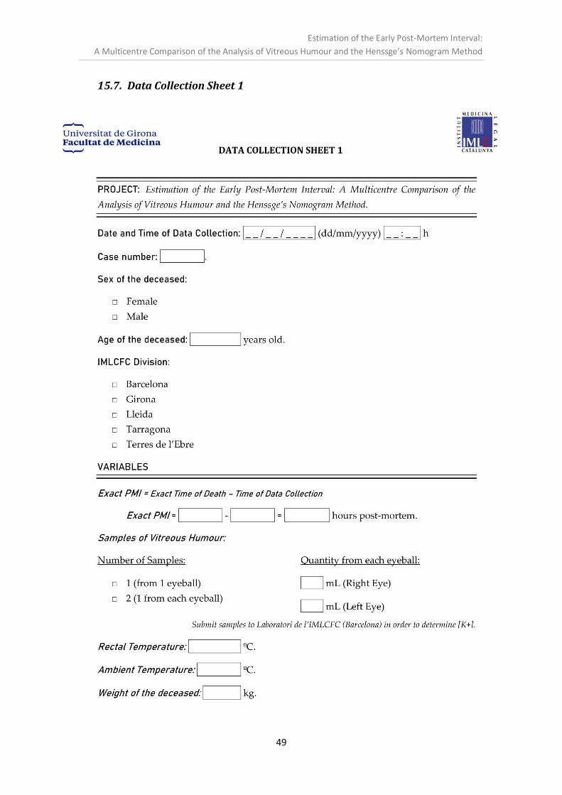
Estimation of the Early Post-Mortem Interval:
A Multicentre Comparison of the Analysis of Vitreous Humour and the Henssge’s Nomogram Method
49
15.7. Data Collection Sheet 1

Estimation of the Early Post-Mortem Interval:
A Multicentre Comparison of the Analysis of Vitreous Humour and the Henssge’s Nomogram Method
50

Estimation of the Early Post-Mortem Interval:
A Multicentre Comparison of the Analysis of Vitreous Humour and the Henssge’s Nomogram Method
51
15.8. Data Collection Sheet 2

Estimation of the Early Post-Mortem Interval:
A Multicentre Comparison of the Analysis of Vitreous Humour and the Henssge’s Nomogram Method
52

Estimation of the Early Post-Mortem Interval:
A Multicentre Comparison of the Analysis of Vitreous Humour and the Henssge’s Nomogram Method
53

Estimation of the Early Post-Mortem Interval:
A Multicentre Comparison of the Analysis of Vitreous Humour and the Henssge’s Nomogram Method
54
Copyright © 2022 FDOKUMEN