Risk Analysis, Vol. 30, No. 3, 2010 DOI: 10.1111/j.1539-6924.2009.01336.x

Perspective

Conundrums with Uncertainty Factors

Roger Cooke∗

The practice of uncertainty factors as applied to noncancer endpoints in the IRIS databaseharkens back to traditional safety factors. In the era before risk quantification, these wereused to build in a “margin of safety.” As risk quantification takes hold, the safety factormethods yield to quantitative risk calculations to guarantee safety. Many authors believe thatuncertainty factors can be given a probabilistic interpretation as ratios of response rates, andthat the reference values computed according to the IRIS methodology can thus be con-verted to random variables whose distributions can be computed with Monte Carlo methods,based on the distributions of the uncertainty factors. Recent proposals from the National Re-search Council echo this view. Based on probabilistic arguments, several authors claim thatthe current practice of uncertainty factors is overprotective. When interpreted probabilisti-cally, uncertainty factors entail very strong assumptions on the underlying response rates. Forexample, the factor for extrapolating from animal to human is the same whether the dosageis chronic or subchronic. Together with independence assumptions, these assumptions en-tail that the covariance matrix of the logged response rates is singular. In other words, theaccumulated assumptions entail a log-linear dependence between the response rates. Thisin turn means that any uncertainty analysis based on these assumptions is ill-conditioned; iteffectively computes uncertainty conditional on a set of zero probability. The practice of un-certainty factors is due for a thorough review. Two directions are briefly sketched, one basedon standard regression models, and one based on nonparametric continuous Bayesian beliefnets.

KEY WORDS: Benchmark dose; LOAEL; NOAEL; uncertainty factors

1. INTRODUCTION

The method of uncertainty factors(1) harkensback to the engineering practice of safety factors. Ifthe reference load for an engineered structure is X,then engineers may design the structure to withstandload 3X, using a safety factor of 3 to create a mar-gin of safety. If the structure functions in a corro-sive environment, another factor would be multipliedto guarantee safety, and another factor for heat, an-other factor for vibrations, etc. The choice of values is

∗Address correspondence to Roger Cooke, Resources for theFuture, Washington, DC, and Department of Mathemat-ics, Delft University of Technology, Delft, The Netherlands;cooke@rff.org.

simply based on “good engineering practice,” that is,what has worked in the past. Although safety factorsare still common in engineering, they are giving wayto probabilistic design in many applications. The rea-son is that compounding safety factors quickly leadsto overdesigning. Compounding safety margins forspaceflight systems may render them too heavy to fly.As our understanding of the system increases, it be-comes possible to guarantee the requisite safety byleveraging our scientific understanding of the mate-rials and processes. That of course requires formu-lating clear probabilistic safety goals, and developingthe techniques to demonstrate compliance.

The engineering community has never soughtto account for uncertainty by treating safety factors

330 0272-4332/10/0100-0330$22.00/1 C© 2009 Society for Risk Analysis

Conundrums with Uncertainty Factors 331

as random variables and assigning them (marginal)distributions; such an approach would not counteractthe overdesigning inherent in safety factors. Manyauthors, including the recent NAS report Science andDecisions (pp. 159 ff)(2) have advocated just such aprobabilistic approach.

EPA’s flagship resource for risk of exposure tohazardous chemicals, the Integrated Risk Informa-tion System (IRIS), uses uncertainty factors as safetyfactors. For noncancer risks, the goal is to derivea reference dose (RfD) or reference concentration(RfC). These “reference values” have been basedon a “no observed adverse effect level” (NOAEL)or lowest observable adverse effect level (LOAEL).The reference dose methodology is applied in sev-eral programs within EPA, including acute refer-ence exposure (ARE), acute exposure guideline level(AEGL), Office of Pesticide Programs procedures,Office of Water (OW) Health Advisories (HA), andthe Agency for Toxic Substances and Disease Reg-istry (ATSDR) Minimal Risk Levels (MRL). Theseprograms have developed different approaches tosetting acute, short-term, and longer-term referencevalues. Efforts are underway to incorporate these dif-ferent values within the integrated risk informationsystem (IRIS) database.

As pointed out by the WHO,(3) the NOAEL isnot a biological threshold, and may either under- oroverestimate a true biological threshold. More re-cently, the benchmark dose (BMD) or lower confi-dence limit of the benchmark dose (BMDL) havebeen used as a point of departure for deriving ref-erence values. The effective dose at which r% of theexposed subjects respond, EDr is another indicatorsometimes used as a point of departure. The regula-tory history is sketched in Reference 4. According toReference 5, the current definition of the RfD is

RfD: an estimate (with uncertainty spanning per-haps an order of magnitude) of a daily oralexposure to the human population (includingsensitive subgroups) that is likely to be with-out appreciable risk of deleterious effects dur-ing a lifetime. It can be derived from a NOAEL,LOAEL, or BMD, with UFs generally appliedto reflect limitations of the data used. Generallyused in EPA’s noncancer health assessments.

The same document proposes a revised definition.

Reference Value: an estimate of an exposure, des-ignated by duration and route, to the humanpopulation (including susceptible subgroups)

that is likely to be without an appreciable riskof adverse health effects over a lifetime. It is de-rived from a BMDL, a NOAEL, a LOAEL, oranother suitable point of departure, with uncer-tainty/variability factors applied to reflect limita-tions of the data used.

The reference value is obtained by dividing apoint of departure by uncertainty factors1 (a typicaldefault value is 10) to account for uncertainty fromvarious sources. These sources, with notion used inIRIS are

1. extrapolation from LOAEL to NOAEL(UFL),

2. data sparseness (UFD: extrapolation frompoor to rich data contexts)

3. interspecies extrapolation (UFA: extrapola-tion from animal to humans)

4. sensitive human subpopulations (UFH), and5. subchronic to chronic dosage (UFS: extrapo-

lation from subchronic to chronic dosage).

The definition makes use of probabilistic andquantitative language as “likely” and “appreciablerisk.” Although this suggests a quantitative interpre-tation, none has been proposed to date. To indicatehow indeterminate words like “appreciable risk” and“likely” can be, consider the “Guidance Notes forLead Authors of the IPCC Fourth Assessment Re-port on Addressing Uncertainties”(7) issued by theIntergovernmental Panel on Climate Change, repro-duced as Table I.

Does exposure at the reference value entail a66% probability of being without appreciable risk?Reference value exposure to 100 substances actingindependently would then entail a 10−18 probabilityof avoiding “appreciable risk.” Being “virtually cer-tain” for each of 100 independent chemicals wouldstill entail only a 37% chance of avoiding apprecia-ble risk. Such examples underscore the inevitabilityof quantifying risk.

1 The IRIS database(6) currently defines “uncertainty/variabilityfactor (UFs)” as: “One of several, generally 10-fold, default fac-tors used in operationally deriving the RfD and RfC from experi-mental data. The factors are intended to account for (1) variationin susceptibility among the members of the human population(i.e., interindividual or intraspecies variability); (2) uncertaintyin extrapolating animal data to humans (i.e., interspecies uncer-tainty); (3) uncertainty in extrapolating from data obtained in astudy with less-than-lifetime exposure (i.e., extrapolating fromsubchronic to chronic exposure); (4) uncertainty in extrapolatingfrom a LOAEL rather than from a NOAEL; and (5) uncertaintyassociated with extrapolation when the database is incomplete.”

332 Cooke

Table I. Likelihood Table from IPCC Fourth AssessmentReport on Addressing Uncertainties

Likelihood of theTerminology Occurrence/Outcome

Virtually certain >99% probability of occurrenceVery likely >90% probabilityLikely >66% probabilityAbout as likely as not 33–66% probabilityUnlikely <33% probabilityVery unlikely <10% probabilityExceptionally unlikely <1% probability

There has been much work at giving a proba-bilistic interpretation of the UFs. Many authors(8−18)

envisage what might be called a Random Chem-ical approach. Several authors adduce propertiesbased on log-normal distributions. Insightful stud-ies(19,20) suggest that uncertainty factors are indepen-dent log-normal variables. Combining uncertaintyfactors involves multiplying the median values, andcombining the “error factors”2 according to theformula KS×A = exp(1.6449 × √

(σ 2S + σ 2

A)), whereσ 2

S and σ 2A are the variances of ln(UFS) and ln(UFA),

respectively. Thus, UFS × UFA is a log-normal var-iable with median(UFS × UFA) = median(UFS) ×median(UFA), and 95 percentile given by median(UFS × UFA) × KS×A. If UFS and UFA each havean error factor of 10, then the error factor of UFS ×UFA is not 100 but 25.95. Several authors suggest thatmultiplying uncertainty factors might overprotect.3

2 Factors that multiply and divide the median of a log-normal dis-tribution to obtain the 5 and 95 percentiles are termed error fac-tors in the technical risk literature.(23)

3 “One of the crucial assumptions affecting how uncertainty fac-tors (UFs) are operationally implemented is that they are inde-pendent of each other. This assumption of independence has ledto the conclusion that the collective uncertainty is the product ofall the individual uncertainty factors” (Ref. 14, p. 44). “Becausenot all true differences are expected to be at their extremes si-multaneously, reducing an observed exposure value by a productof default uncertainty factors may lead to undue conservatism”(Ref. 19, p. 190). “Sound combination of extrapolation factorsstill is an unresolved task in risk assessment. In case of simplemultiplication to an overall extrapolation factor this may lead tooverly conservative human limit values, if all maximal single fac-tors are used simultaneously. In addition, multiplication of singleextrapolation factors would only be correct for independent pa-rameters” (Ref. 3, p. 97). “Because of the application of variousuncertainty factors that are multiplied with each other, the stan-dard method for deriving acceptable human limit values is gener-ally considered to be conservative. Indeed, when each individualuncertainty factor by itself is regarded to reflect a worst case sit-uation, their product, i.e. the overall uncertainty factor, will tendto be overly conservative” (Ref. 12, p. 787).

Recent proposals from the National Research Coun-cil(2) are based on the random chemical approach,and inherit its problems. For data on response ratiossee References 21 and 22.

Section 2 identifies assumptions that the currentpractice imposes on a probabilistic interpretation ofuncertainty factors. The random chemical model isformulated in Section 3, and Section 4 shows that thelogged covariance matrix of response rates is singu-lar. Suggestions for moving beyond uncertainty fac-tors are explored in Section 5.

2. ASSUMPTIONS UNDERLYINGUNCERTAINTY FACTORS

A probabilistic model for uncertainty factorswould consist of a sample space and a set of randomvariables together with assumptions on their jointdistribution such that relations between these ran-dom variables reflect the operations that practition-ers perform with uncertainty factors. Under the ran-dom chemical model, uncertainty factors are randomvariables reflecting response ratios of randomly sam-pled toxic substances. Distributions of these ratiosare used to draw inferences about new or untestedchemicals. The operations performed with uncer-tainty factors entail assumptions on their joint dis-tribution. The prevailing assumptions are presentedinformally in this section, precise versions are used inSection 3.

We consider a point of departure (POD), whichmay be either a BMD, a LOAEL, a NOAEL, oran effective dose for response of r% of the popula-tion (EDr). The relevant assumptions are (“UFs” de-notes “uncertainty factors,” not to be confused with“UFS”):

1. The UFs are independent random variables.2. The extrapolation expressed by a UF is in-

dependent of other extrapolations. That is,the UF for extrapolating from poor to richdata contexts does not depend on whether theextrapolation concerns chronic or subchronicdose. The extrapolation from subchronic tochronic dosage does not depend on whetherthis is applied to humans or animals, or to thepoor/rich data contexts,4 etc.

4 Subchronic exposure is defined as:(6) “Repeated exposure by theoral, dermal, or inhalation route for more than 30 days, up to ap-proximately 10% of the life span in humans (more than 30 daysup to approximately 90 days in typically used laboratory animalspecies).” Chronic exposure is defined as: “Repeated exposure

Conundrums with Uncertainty Factors 333

3. The conditional distribution of a human ref-erence value, given an observed (unextrap-olated) POD, is obtained by dividing theobserved POD by the product of the UFs cor-responding to the required extrapolations.

3. RANDOM CHEMICAL MODEL

We illustrate the random chemical model for theextrapolations poor-to-rich, subchronic-to-chronic,and animal-to-human. Other extrapolations couldserve equally well to illustrate the issues. Suppose werandomly sample toxic chemical t from a representa-tive set of toxic substances. For each t, we imaginethat we have values for the POD for animals at eachdosage regime (chronic, subchronic; C, S), for eachdata context (poor, rich; P, R), and for two species(animal, human; A, H). Hence if HC(t) is the refer-ence value for t, that is, the chronic dose that is likelyto be without appreciable lifetime risk, we may al-ways write an equation of the form:

HC(t) = ASP(t)ASR(t)ASP(t)

ACR(t)ASR(t)

HC(t)ACR(t)

. (1)

If we consider t as a randomly drawn chemical,which, following convention, we denote with uppercase T, we can write Equation (1) as an equation ofrandom variables:

HC(T) = ASP(T)ASR(T)ASP(T)

ACR(T)ASR(T)

HC(T)ACR(T)

. (2)

by the oral, dermal, or inhalation route for more than approxi-mately 10% of the life span in humans (more than approximately90 days to 2 years in typically used laboratory animal species).”UA is defined as follows: “Use an additional 10-fold factor whenextrapolating from valid results from long term studies on ex-perimental animals when results of studies of human exposureare not available or are inadequate” and UC: “Use an additional10-fold factor when extrapolating from less than chronic resultson experimental animals when there are no useful long-term hu-man data.” These definitions would not tell us how to extrapo-late from human subchronic studies, nor from animal subchronicto animal chronic. Such extrapolations are surely less prevalent,though not excluded, as the definitions of subchronic and chronicdosages make clear. The absence of separate uncertainty factors,for example, for subchronic-to-chronic for animals and for hu-mans, suggests that Equation (1) is implicitly assumed. Indeed,Swartout et al. (Ref. 11, p. 275) write: “Within the current RfDmethodology, UFC [here, UFS] does not consider differencesamong species, endpoints, or severity of effects, the same factoris applied in all cases.” Because of the rarity of relevant humandata, the same authors suggest the use of other endpoints as sur-rogates in estimating UA.

If we now write:

UFD = ASP(T)ASR(T)

, UFS = ASR(T)ACR(T)

, UFA = ACR(t)HC(t)

,

(3)

then it appears that have interpreted UFs as randomvariables based on the random chemical model:

HC(T) = ASP(T)UFD × UFS × UFA

. (4)

Equation (4) reflects an assumption noted bymany authors, namely, that the UFs as random vari-ables must be independent. However, Equation (4)involves more assumptions that have not receivedample attention. Suppose we observe for a giventoxic substance t that ASP(t) = 30 [units]. We use30/(UFD × UFS × UFA) as the conditional distribu-tion of HC(T) given ASP(T) = 30. This must holdfor any observed value, thus ASP(T) must be inde-pendent of UFD × UFS × UFA.5 Barring pathologi-cal situations, this means that ASP(T) is independentof each of these UFs.

Note that these conditionalization assumptionsalways apply from “more easily measured to moredifficult to measure.” They do not apply in the otherdirection. Letting “⊥” denote independence, if X ⊥X/Y and also Y ⊥ X/Y, then it is easy to show thatX/Y must be constant.6

4. IMPLICATIONS OF ASSUMPTIONS

These independence assumptions are quitestrong and have consequences. Consider the state-ment that:

ASP(T) ⊥ UFD. (5)

Note that ASR(T) = ASP(T)/UFD. Taking logsof both sides:

Ln(ASR(T) = Ln(ASP(T)) − Ln(UF D). (6)

5 Rehearsing elementary probability, suppose we wish to expressthe uncertainty in random variable X, given that another ran-dom variable Y takes the value y. One way of modeling this isto write X as a function g(Y, Z) of Y and some other randomvariable Z. If Z is independent of Y, then the conditional distri-bution (X | Y = y) of X given Y = y is the distribution of the ran-dom variable g(y, Z). If Y and Z are not independent, then wemust use the conditional distribution (Z | Y = y) when comput-ing the distribution of g. In this case X = HC(T), Y = ASP(T),Z = UFA(T) × UFS(T) × UFD, and g(Y, Z) = Y/Z. To justifythe type of conditionalization for which the UFs are intended, wemust have ASP(T) independent of {UFA(T), UFS(T), UFD(T)}.

6 Take logs, write out the covariances, and infer that σ 2ln(X)−ln(Y) =

0.

334 Cooke

ASP(T) ⊥ UFD entails also Ln(ASP(T) ⊥ Ln(UFD); and that:

VAR(Ln(ASR(T)) = VAR(Ln(ASP(T)))

+ VAR(Ln(UF D)). (7)

This says that the variance of logged animalPODs based on subchronic dosage and rich data setsis strictly greater than the variance of logged animalPODs based on a subchronic dosage with poor datacontexts; the same holds for chronic dosage. Thisseems counterintuitive. Similarly, ASP(T) ⊥ UFS im-plies that VAR[Ln(ACP(T))] > VAR[Ln(ASP(T))],and the same holds for rich data contexts. This meansthat the variance of the logged animal chronic val-ues is strictly greater than the variance of the loggedanimal subchronic value, which is at odds with state-ments in the Cancer Guidelines.7 This underscoresthe importance of identifying underlying assump-tions.

We now demonstrate the singularity of the co-variance matrix of logged terms in the UFs. It suf-fices to consider only the extrapolation from poor torich data contexts, and from subchronic to chronicdosages, all for animal PODs. We could equally wellhave chosen UFL and UFA; the argument would beidentical. To lighten the notation in this section, letSP denote the animal value of the POD under sub-chronic dosage in a poor data context, CR the ani-mal POD under chronic dosage in a rich data context,and let SR and CP be defined similarly. Each of theseis considered as a random variable whose values aredetermined by randomly sampling a toxic substancefrom a representative set.

The basic equations are:

CR = SP × (SR/SP) × (CR/SR)

= SP/(UFD × U DS) (8)

CR = CP × (CR/CP) = CP/UFD. (9)

The same UF is applied for extrapolating frompoor to rich data contexts, regardless whether thedosage is chronic or subchronic. This means thatUFD has a distribution that can be measured in twoways:

7 “Uncertainty usually increases as the duration becomes shorterrelative to the averaging duration or the intermittent doses be-come more intense than the averaged dose. Moreover, doses dur-ing any specific susceptible or refractory period would not beequivalent to doses at other times.”(3,4,24)

UFD ∼ SPSR

(10)

UFD ∼ CPCR

. (11)

Similarly, the UF for extrapolating from sub-chronic to chronic is used for both rich and poor datacontexts, hence:

UFS ∼ SPCP

(12)

UFS ∼ SRCR

. (13)

We use the following notation:

A= VAR(ln(SP)),

B = VAR(ln(SR)),

C = VAR(ln(CP)),

D = VAR(ln(CR)).

If two variables are independent, then also thelogs of these variables are independent. If X is inde-pendent of Y, then X is also independent of 1/Y. Thefollowing independence statements are assumed bythe UF methodology, under a probabilistic interpre-tation:

I.1 SP ⊥ SP/SR (enable conditionalization inEquation (8))

I.2 SP ⊥ SR/CR (enable conditionalization inEquation (8))

I.3 SP/SR ⊥ SR/CR (UFD ⊥ UFS)I.4 SP ⊥ CP/CR (enable conditionalization in

Equation (8) with Equation (11))I.5 CP ⊥ CP/CR (enable conditionalization in

Equation (9))I.6 CP ⊥ SP/SR (enable conditionalization in

Equation (9) with Equation (10))I.7 SR/CR ⊥ CP/CR (UFS ⊥ UFD)

If two variables are independent, then their co-variance is zero. Let Cov(X,Y) denote the covari-ance of X and Y. Taking logs of I.1–I.7, and settingcovariances of independent variables equal to zero,using the linearity of covariance, we find:

Conundrums with Uncertainty Factors 335

Table II. Log Covariance Matrix

Ln(SP) Ln(SR) Ln(CP) Ln(CR)

Ln(SP) A A A ALn(SR) A B A BLn(CP) A A C CLn(CR) A B C B + C − A

I.1 ⇒ A= Cov(ln(SP), ln(SR)),

I.2 and I.1 ⇒ A= Cov(ln(SP), ln(CR)),

I.3 and I.1 and I.2 ⇒ B = Cov(ln(SR), ln(CR)),

I.4 and I.1 and I.2 ⇒ A= Cov(ln(SP), ln(CP)),

I.5 ⇒ C = Cov(ln(CP), ln(CR)),

I.6 and I.4 ⇒ A= Cov(ln(CP), ln(SR)),

I.7 and I.6 and I.5

and I.3 ⇒ D = B + C − A.

We bring these relations together in the follow-ing covariance matrix.

Observe that the second plus third rows, minusthe first row equals the fourth row. The determinantof this matrix is zero, meaning that there is a linearrelationship between the variables. Using VAR(X +Y) = VAR(X) + VAR(Y) + 2Cov(X,Y), with thevalues in Table II it follows that:

VAR(ln(CR) + ln(SP) − ln(SR) − ln(CP)) = 0.

(14)

In other words:

CR = SR × CP/SP. (15)

Rearranging, we may write this as CR/CP =SR/SP. This says that the two random variables inEquations (10) and (11) must actually be the samevariable. This means that if we actually knew the val-ues SP(t), CP(t), and SR(t), we could compute CR(t).Similar singularities arise if we consider other pairsof UFs.

5. HOW FORWARD?

The first step forward is to realize that the cur-rent system will not admit a probabilistic interpreta-tion and that fundamental changes are required if wewish to account for uncertainty in reference values.Ultimately, for important chemicals, we should liketo combine animal data, in vitro human data, and epi-demiological data from natural experiments to derivedose-response relations with uncertainty quantifica-

tion. However, there will always be a need to eval-uate new potentially toxic chemicals based on theirsimilarity to other chemicals and meager experimen-tal data. We should like a simple method that:

1. Yields predictions of toxicological indica-tors with uncertainty via a valid probabilisticmechanism.

2. Is based on a random chemical model, regard-ing a new chemical as a random sample froma reference distribution of chemicals.

3. Is nondisruptive.

This last desideratum is very important, andhas received insufficient attention. Regulatory bod-ies cannot turn on a dime, but must contend with alegacy of accepted practice. The foregoing suggeststhat a probabilistically valid inference system will bequite different from the current system. Nonetheless,to meld with current practice, it must initialize on thecurrent system, and allow this system to evolve in ameasured fashion.

We can use the IRIS database to obtain a ref-erence set of substances, perhaps supplemented withstructured expert judgment. These reference valuesserve to define a population of toxic substances fromwhich a new substance is regarded as a random sam-ple. The idea is simply to discard the UF method-ology, but to retain the results of that method as areference distribution to initialize the new system.The reference distribution can further evolve underthe new regime, but the changes in toxicity indicatorvalues will be nondisruptive. There are at least twoways of leveraging such a reference set to draw infer-ences on new substances: standard log-linear regres-sion and nonparametric Bayesian belief nets.

5.1. Standard (Log) Linear Regression

To render this discussion more intuitive, we fo-cus on animal (A) and human (H) responses atchronic (C) and subchronic (S) dosages. Supposewe are interested in predicting ln(HC)(t∗) for a newtoxic substance t∗, and we can estimate Cov(ln(HC),ln(AC)), and σ 2(ln(AC)) from a large data set oftoxic substances. Translating all variables to havemean zero, the linear least squares predictor (llsp) ofln(HC) based on ln(AC) would be:

llsp(ln(HC)(t∗)| ln(AC)(t∗)) = Cov(ln(HC),

ln(AC)) × (1/σ 2(ln(AC))) × ln(AC)(t∗).

336 Cooke

If ln(AC)(t∗) is known, this is a predictor ofln(HC)(t∗), not a random variable. We might try tothink of σ 2(ln(AC))/Cov(ln(HC), ln(AC)) as an un-certainty factor, but these would not behave as un-certainty factors in the IRIS methodology. To giveone illustration, suppose we observed ln(AS)(t∗) inaddition to ln(AC)(t∗). The IRIS method would notuse the additional information regarding AS(t∗), butwould simply use AC(t∗)/UA. However, following thetheory of linear models, we should have:

llsp((ln(HC)(t∗)| ln(AC)(t∗),

ln(AS)(t∗)) = llsp(ln(HC)(t∗)| ln(AC)(t∗))

+ llsp[ln(HC)(t∗)| ln(AC)(t∗)

− llsp(ln(AC)(t∗)| ln(AS)(t∗))].

In other words, we add the llsp of ln(HC)(t∗)based on ln(AC)(t∗) to the llsp of ln(HC)(t∗)based on the residual ln(AC)(t∗) − llsp(ln(AC)(t∗) |ln(AS)(t∗)).

We can extract the variance of the llsp; for ar-bitrary random vectors X, Y, we have (the varianceand covariance terms now denote matrices):

σ 2(llsp(Y | X) = Cov(Y, X)(σ 2(X))−1Cov(X, Y).

We also obtain the variance of the residual as:

σ 2(Y − llsp(Y | X)) = σ 2(Y) − σ 2(llsp(Y | X).

Note that the last two variances do not dependon the value of the conditioning variable X. In gen-eral, the variance of the residual is not the conditionalvariance of Y given X, and we do not get the condi-tional distribution of Y given X. In many cases, wemay actually be interested in the distribution of hu-man values given observed animal values, especiallyif these observed values are in the tails of their re-spective distributions. Such considerations drive us inthe direction of Bayesian belief nets.

5.2. Nonparametric Continuous BayesianBelief Nets

Nonparametric continuous Bayesian belief nets(NPCBBNs) build a joint density.(25) A full de-scription is inappropriate here; suffice to say thatNPCBBNs are based on empirical marginal distri-butions and empirical rank correlations; they builda joint density by modeling the copula that realizesthese empirical rank correlations. In principle anycopula can be used, but in practice the joint normalcopula is preferred, as it enables rapid conditional-ization. Roughly, this means that the rank depen-

dence structure is modeled as that of a joint normaldistribution. This hypothesis can be tested, based onthe sampling distribution of the determinant of thenormal rank correlation matrix. The marginal distri-butions and rank correlations are not modeled, buttaken directly from data; hence they do not form partof the hypothesis being tested. If the normal copulahypothesis is not rejected, then we can proceed toconditionalize any variable on any set of values ofother variables.

5.2.1. Using NPCBBNs for Inference on Toxicity

A BBN is a mechanism for encoding inferences.Drawing an inference from data is performed by con-ditionalizing a BBN on the data; the distribution cap-tured in the BBN is updated with current data. BBNsare simply a perspicuous way of visualizing com-plex inference patterns. Continuous nonparametricBBNs enable this inference based on an initial dataset. With the normal copula, very large problemswith very complex inference structures can be han-dled analytically, so that the inferences are effec-tively instantaneous. The marginal distributions andrank correlation structure is read from the data; theonly assumption is that these rank correlations arecompatible with the normal copula. This is a muchweaker assumption than that underlying standard re-gression models, namely, that error terms are inde-pendent and normally distributed.

To compare the BBN approach to standard re-gression modeling, suppose that we are interested insome probabilistic response in animals (A) and hu-mans (H) at chronic (C) and subchronic (S) dosage.As before, this might be an RfD, RfC, BMD, oran ED10 or indeed any other indicator. It could bean ED10 for subchronic dosage of animals, ED50

for chronic dosage for animals, an RfD for chronichuman dosage, and a BMD for subchronic humandosage. All that matters is that we have a list of,say, 100 toxic substances filled in as illustrated inTable III. The units in each column must bethe same, but need not be the same acrosscolumns.

When the inference engine is “seeded” in thisway, we can apply it to some new chemical thatwe regard is a random sample from the populationof chemicals from which the chemicals inTable IIIare randomly drawn. We guarantee thereby that theinferences for new chemicals will reflect the rela-tions between the probabilistic response variablescaptured in Table III.

Conundrums with Uncertainty Factors 337

Table III. Illustrative Input for BBN

Probabilistic Response: Probabilistic Response: Probabilistic Response: Probabilistic ResponseAnimal, Subchronic Animal Chronic Human Subchronic Human Chronic

Toxic Chem. 1 20 [AS units] 15 [AC units] 4[HS units] 2[HC units]Toxic Chem. 2 45[AS units] 30[AC units] 30[HS units] 26[HC units]Toxic Chem. 3 30[AS units] 35[AC units] 20[HS units] 14[HC units]

. . . . . . . . . . . . . . .

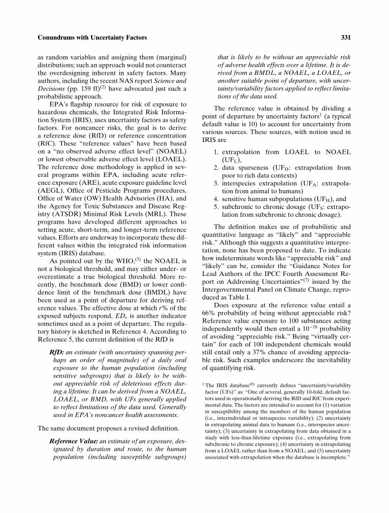
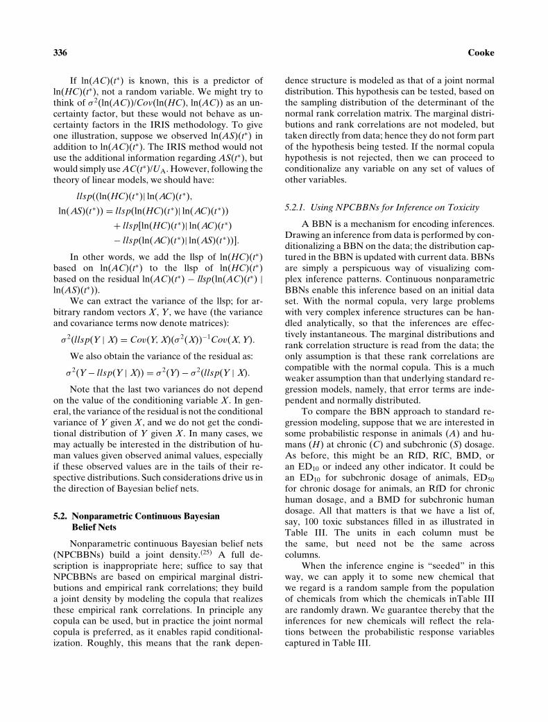
Fig. 1. Bayesian belief net for P, Animal, Subchronic (AS); P,Animal, Chronic (AC)); P, Human, Subchronic, ((HS)); andP, Human, Chronic (HC)), distributions over set of (fictitious)toxic substances; (conditional) rank correlations as inferred fromTable II are shown.

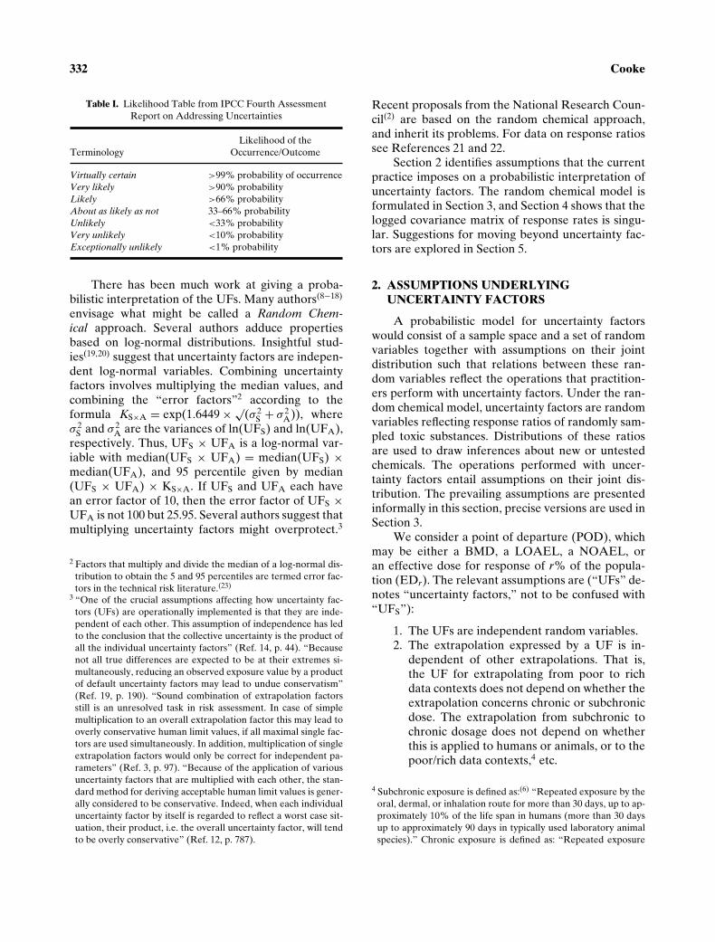
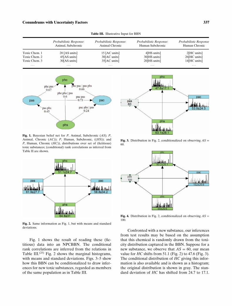
Fig. 2. Same information as Fig. 1, but with means and standarddeviations.

Fig. 1 shows the result of reading these (fic-titious) data into an NPCBBN. The conditionalrank correlations are inferred from the relations inTable III.(25) Fig. 2 shows the marginal histograms,with means and standard deviations. Figs. 3–5 showhow this BBN can be conditionalized to draw infer-ences for new toxic substances, regarded as membersof the same population as in Table III.

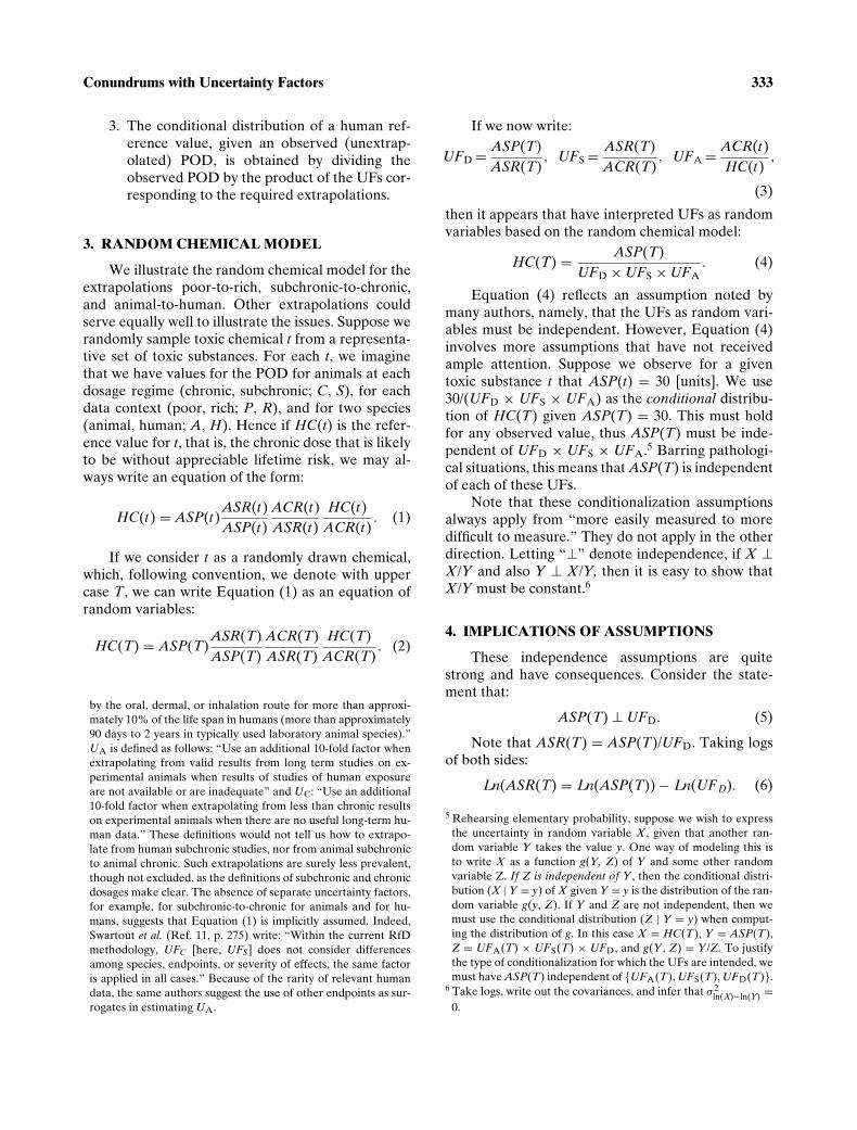
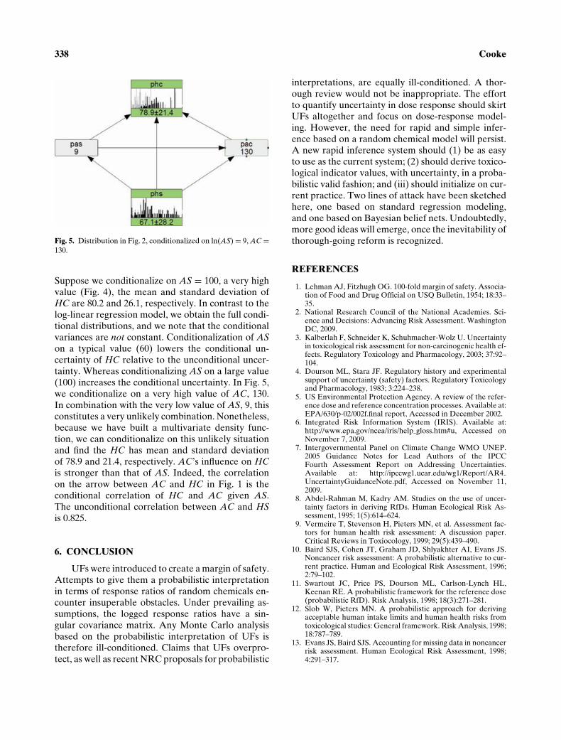
Fig. 3. Distribution in Fig. 2, conditionalized on observing AS =60.

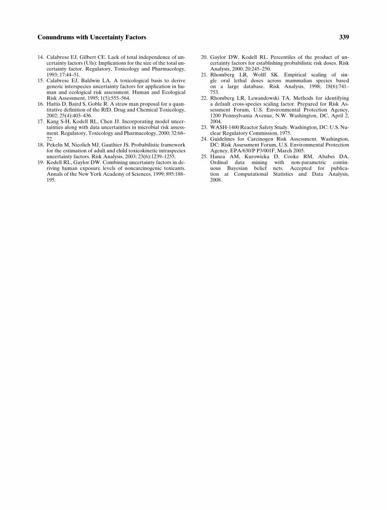
Fig. 4. Distribution in Fig. 2, conditionalized on observing AS =100.

Confronted with a new substance, our inferencesfrom test results may be based on the assumptionthat this chemical is randomly drawn from the toxi-city distribution captured in the BBN. Suppose for anew substance, we observe that AS = 60, our meanvalue for HC shifts from 51.1 (Fig. 2) to 47.6 (Fig. 3).The conditional distribution of HC giving this infor-mation is also available and is shown as a histogram;the original distribution is shown in gray. The stan-dard deviation of HC has shifted from 24.7 to 17.1.

338 Cooke

Fig. 5. Distribution in Fig. 2, conditionalized on ln(AS) = 9, AC =130.

Suppose we conditionalize on AS = 100, a very highvalue (Fig. 4), the mean and standard deviation ofHC are 80.2 and 26.1, respectively. In contrast to thelog-linear regression model, we obtain the full condi-tional distributions, and we note that the conditionalvariances are not constant. Conditionalization of ASon a typical value (60) lowers the conditional un-certainty of HC relative to the unconditional uncer-tainty. Whereas conditionalizing AS on a large value(100) increases the conditional uncertainty. In Fig. 5,we conditionalize on a very high value of AC, 130.In combination with the very low value of AS, 9, thisconstitutes a very unlikely combination. Nonetheless,because we have built a multivariate density func-tion, we can conditionalize on this unlikely situationand find the HC has mean and standard deviationof 78.9 and 21.4, respectively. AC’s influence on HCis stronger than that of AS. Indeed, the correlationon the arrow between AC and HC in Fig. 1 is theconditional correlation of HC and AC given AS.The unconditional correlation between AC and HSis 0.825.

6. CONCLUSION

UFs were introduced to create a margin of safety.Attempts to give them a probabilistic interpretationin terms of response ratios of random chemicals en-counter insuperable obstacles. Under prevailing as-sumptions, the logged response ratios have a sin-gular covariance matrix. Any Monte Carlo analysisbased on the probabilistic interpretation of UFs istherefore ill-conditioned. Claims that UFs overpro-tect, as well as recent NRC proposals for probabilistic

interpretations, are equally ill-conditioned. A thor-ough review would not be inappropriate. The effortto quantify uncertainty in dose response should skirtUFs altogether and focus on dose-response model-ing. However, the need for rapid and simple infer-ence based on a random chemical model will persist.A new rapid inference system should (1) be as easyto use as the current system; (2) should derive toxico-logical indicator values, with uncertainty, in a proba-bilistic valid fashion; and (iii) should initialize on cur-rent practice. Two lines of attack have been sketchedhere, one based on standard regression modeling,and one based on Bayesian belief nets. Undoubtedly,more good ideas will emerge, once the inevitability ofthorough-going reform is recognized.

REFERENCES

1. Lehman AJ, Fitzhugh OG. 100-fold margin of safety. Associa-tion of Food and Drug Official on USQ Bulletin, 1954; 18:33–35.

2. National Research Council of the National Academies. Sci-ence and Decisions: Advancing Risk Assessment. WashingtonDC, 2009.

3. Kalberlah F, Schneider K, Schuhmacher-Wolz U. Uncertaintyin toxicological risk assessment for non-carcinogenic health ef-fects. Regulatory Toxicology and Pharmacology, 2003; 37:92–104.

4. Dourson ML, Stara JF. Regulatory history and experimentalsupport of uncertainty (safety) factors. Regulatory Toxicologyand Pharmacology, 1983; 3:224–238.

5. US Environmental Protection Agency. A review of the refer-ence dose and reference concentration processes. Available at:EPA/630/p-02/002f.final report, Accessed in December 2002.

6. Integrated Risk Information System (IRIS). Available at:http://www.epa.gov/ncea/iris/help gloss.htm#u, Accessed onNovember 7, 2009.

7. Intergovernmental Panel on Climate Change WMO UNEP.2005 Guidance Notes for Lead Authors of the IPCCFourth Assessment Report on Addressing Uncertainties.Available at: http://ipccwg1.ucar.edu/wg1/Report/AR4UncertaintyGuidanceNote.pdf, Accessed on November 11,2009.

8. Abdel-Rahman M, Kadry AM. Studies on the use of uncer-tainty factors in deriving RfDs. Human Ecological Risk As-sessment, 1995; 1(5):614–624.

9. Vermeire T, Stevenson H, Pieters MN, et al. Assessment fac-tors for human health risk assessment: A discussion paper.Critical Reviews in Toxiocology, 1999; 29(5):439–490.

10. Baird SJS, Cohen JT, Graham JD, Shlyakhter AI, Evans JS.Noncancer risk assessment: A probabilistic alternative to cur-rent practice. Human and Ecological Risk Assessment, 1996;2:79–102.

11. Swartout JC, Price PS, Dourson ML, Carlson-Lynch HL,Keenan RE. A probabilistic framework for the reference dose(probabilistic RfD). Risk Analysis, 1998; 18(3):271–281.

12. Slob W, Pieters MN. A probabilistic approach for derivingacceptable human intake limits and human health risks fromtoxicological studies: General framework. Risk Analysis, 1998;18:787–789.

13. Evans JS, Baird SJS. Accounting for missing data in noncancerrisk assessment. Human Ecological Risk Assessment, 1998;4:291–317.

Conundrums with Uncertainty Factors 339

14. Calabrese EJ, Gilbert CE. Lack of total independence of un-certainty factors (Ufs): Implications for the size of the total un-certainty factor. Regulatory, Toxicology and Pharmacology,1993; 17:44–51.

15. Calabrese EJ, Baldwin LA. A toxicological basis to derivegeneric interspecies uncertainty factors for application in hu-man and ecological risk assessment. Human and EcologicalRisk Assessment, 1995; 1(5):555–564.

16. Hattis D, Baird S, Goble R. A straw man proposal for a quan-titative definition of the RfD. Drug and Chemical Toxicology,2002; 25(4):403–436.

17. Kang S-H, Kodell RL, Chen JJ. Incorporating model uncer-tainties along with data uncertainties in microbial risk assess-ment. Regulatory, Toxicology and Pharmacology, 2000; 32:68–72.

18. Pekelis M, Nicolich MJ, Gauthier JS. Probabilistic frameworkfor the estimation of adult and child toxicokinetic intraspeciesuncertainty factors. Risk Analysis, 2003; 23(6):1239–1255.

19. Kodell RL, Gaylor DW. Combining uncertainty factors in de-riving human exposure levels of noncarcinogenic toxicants.Annals of the New York Academy of Sciences, 1999; 895:188–195.

20. Gaylor DW, Kodell RL. Percentiles of the product of un-certainty factors for establishing probabilistic risk doses. RiskAnalysis, 2000; 20:245–250.

21. Rhomberg LR, Wolff SK. Empirical scaling of sin-gle oral lethal doses across mammalian species basedon a large database. Risk Analysis, 1998; 18(6):741–753.

22. Rhomberg LR, Lewandowski TA. Methods for identifyinga default cross-species scaling factor. Prepared for Risk As-sessment Forum, U.S. Environmental Protection Agency,1200 Pennsylvania Avenue, N.W. Washington, DC, April 2,2004.

23. WASH-1400 Reactor Safety Study. Washington, DC: U.S. Nu-clear Regulatory Commission, 1975.

24. Guidelines for Carcinogen Risk Assessment. Washington,DC: Risk Assessment Forum, U.S. Environmental ProtectionAgency, EPA/630/P P3/001F, March 2005.

25. Hanea AM, Kurowicka D, Cooke RM, Ababei DA.Ordinal data mining with non-parametric contin-uous Bayesian belief nets. Accepted for publica-tion at Computational Statistics and Data Analysis,2008.