Recognition criteria vary with fluctuating uncertainty

Joshua A. Solomon # $Optometry Division, Applied Vision Research Centre, City

University London, UK

Patrick Cavanagh # $Laboratoire Psychologie de la Perception, Universite

Paris Descartes and CNRS, Paris, France

Andrei Gorea # $Laboratoire Psychologie de la Perception, Universite

Paris Descartes and CNRS, Paris, France

In distinct experiments we examined memories for orientation and size. After viewing a randomly oriented Gabor patch (or aplain white disk of random size), observers were given unlimited time to reproduce as faithfully as possible the orientation(or size) of that standard stimulus with an adjustable Gabor patch (or disk). Then, with this match stimulus still in view, arecognition probe was presented. On half the trials, this probe was identical to the standard. We expected observers toclassify the probe (a same/different task) on the basis of its difference from the match, which should have served as anexplicit memory of the standard. Observers did better than that. Larger differences were classified as ‘‘same’’ when probeand standard were indeed identical. In some cases, recognition performance exceeded that of a simulated observer subjectto the same matching errors, but forced to adopt the single most advantageous criterion difference between the probe andmatch. Recognition must have used information that was not or could not be exploited in the reproduction phase. Onepossible source for that information is observers’ confidence in their reproduction (e.g., in their memory of the standard).Simulations confirm the enhancement of recognition performance when decision criteria are adjusted trial-by-trial, on thebasis of the observer’s estimated reproduction error.

Keywords: orientation, size, reproduction, recognition, confidence, doubly stochastic noise, decision criteria, accuracy

Citation: Solomon, J. A., Cavanagh, P., & Gorea, A. (2012). Recognition criteria vary with fluctuating uncertainty. Journal ofVision, 12(8):2, 1–13, http://www.journalofvision.org/content/12/8/2, doi:10.1167/12.8.2.

Introduction

In conventional recognition experiments, observerstry their best to remember a standard stimulus, butmemory is not perfect. The precision of those memoriesmay be inferred from their recognition responses usingSignal Detection Theory (SDT) (Green & Swets, 1966),but with one crucial assumption; namely that observersuse the same decision strategy (i.e., criterion) on everytrial. Sophisticated theorists (notably Wickelgren,1968) have already acknowledged that decision criteriamay fluctuate. The problem remains that this fluctua-tion is indistinguishable from memory noise in mostparadigms. Evidence that decision criteria dependsystematically on trial-by-trial feedback was firstpresented by Tanner, Rauk, and Atkinson (1970).Treisman and Williams (1984) later codified severalpreviously reported sequential effects in their CriterionSetting Theory. Our own research is situated within thisalternative tradition. We introduce a paradigm inwhich criterion fluctuation demonstrably improvesrecognition performance.

In our paradigm, criterion fluctuation can beadvantageous only if it complements a similar fluctu-ation in the precision of memory. After 150 years (seep. 82 of Fechner, 1860 & 1966), this idea of variableprecision is only now finding its way into signal-detection models (notably that of van den Berg, Shin,Chou, George, & Ma, 2012). To get a handle on thetrial-by-trial fluctuation in memory noise, we requiredobservers to match their memory of each standard withan adjustable stimulus. We then computed the bestpossible recognition performances, assuming thatreproduction errors reflected a memory noise withconstant precision. The fact that our observers’recognition performances exceeded these predictionsallows us to infer that memory noise has variableprecision. This would be insufficient to allow better-than-prediction recognition if observers’ decision crite-ria did not covary with their memory noise.

Our empirical approach (summed up in the Abstractand detailed in the Methods) consisted of a matching(recollection) task followed by a same/different (recog-nition) task. This approach allows us to characterizedecision strategies for recognition with respect toexplicit representations of the imperfectly recollected

Journal of Vision (2012) 12(8):2, 1–13 1http://www.journalofvision.org/content/12/8/2

doi: 10 .1167 /12 .8 .2 ISSN 1534-7362 � 2012 ARVOReceived December 19, 2011; published August 6, 2012

standards. Such a feat is impossible with standard yes/no procedures. As will be shown, our observers’decision behavior is consistent with a doubly stochasticmemory noise model where observers modulate theirdecision criterion in the recognition phase in inverseproportion with their confidence in their match. To ourknowledge, the present experiments are the first toprovide empirical evidence of a systematic, trial-by-trialmodulation of recognition strategy in accordance withobservers’ confidence in each memory of the standardstimulus.

Methods

Units

In this paper, all Gabor orientations (s, m, m0, and p;see below) have units of degree, clockwise with respectto horizontal. All disk sizes (also s, m, m0, and p) arequantified as logarithms (base 10) of diameter.

Stimuli

Gabor patches or white disks (see Figure 1) werepresented on a 15’’ MacBook Pro computer at acomfortable viewing distance of about 0.5 m. At thisdistance, each Gabor was centered 38 of visual angle tothe left or right of a central fixation spot. The whitedisks were displayed at the same mean eccentricity buttheir positions were randomly jittered, across andwithin trials, 618. Each Gabor was the product of asinusoidal luminance grating and a Gaussian lumi-nance envelope. The grating had a spatial frequency of1.5 cycles per degree and a random spatial phase. TheGaussian envelope had a space constant (r) of 0.5degrees of visual angle. Both grating and envelope had

maximum contrast. The white disks had a luminance of260 cd/m2. Stimuli were presented on a grey, 60 cd/m2

background.

Procedure

On each trial, the standard, a randomly orientedGabor (or a random size white disk), was briefly (200ms) presented on one side of fixation. The observerthen attempted to reproduce its orientation (or size, s)by manipulating another stimulus (the match), subse-quently presented on the opposite side of fixation. Justlike the standard, the match’s initial orientation (orsize, m0) was randomly selected from a uniformdistribution over all orientations (or diameters between1.58 and 3.08). Each press of the ‘‘c’’ key rotated thematch 28 anticlockwise (or reduced its diameter by 2%)and each press of the ‘‘m’’ key rotated it 28 clockwise(or increased its diameter by 2%).1 Gabor phase wasrandomly reselected with each keypress. To indicatesatisfaction with the match’s orientation (or size, m),the observer pressed the space bar, initiating the trial’ssecond, recognition phase. With the match still in view,a probeGabor (or disk) was presented at the location ofthe standard. On 50% of trials the orientation (or size,p) of the probe was identical to s. In the remaining trialsthe orientation (or size) of p was changed with respectto s by a value, 6Ds.2 The value of Ds was heldconstant within each block of trials. In the orientationexperiment, Ds took values of 38, 58, 78, 148, and 218. Inthe size experiment, Ds took values of 0.04, 0.06, and0.08. Observers had to classify p as either ‘‘same’’ or‘‘different’’ with respect to their memory of s. Nofeedback was given. Observers performed two blocks of100 trials at each level of difficulty in a random order.Two additional 50-trial blocks (one with Ds ¼ 38, theother with Ds ¼ 58) were run by the last author in the

Figure 1. Spatiotemporal layout of the displayed and matched stimuli in the orientation (a) and size (b) experiments. In this diagram the

size of the fixation cross and its distance from the standard have been scaled to twice their actual values.

Journal of Vision (2012) 12(8):2, 1–13 Solomon, Cavanagh, & Gorea 2

orientation experiment and were included in allsubsequent analyses.

Observers

Two authors and two naıve observers were run in theorientation experiment. The same two authors andthree naıve observers (one of which, KM, alsoparticipated in the orientation experiment) were runin the size experiment.

Results

Gross indices of reproduction can be obtained bycomputing the standard deviation of each observer’smatching errors (s – m). Across observers, these indiceshad a mean and standard deviation (SD) of 9.68 and0.78, respectively, for orientation,3 and 0.048 and 0.013,respectively, for size (see Tables SM1 and SM2 inSupplementary material). Comparable values for ori-entation have been obtained under similar conditions(e.g., Tomassini, Morgan, & Solomon, 2010), but moreprecise reproduction has also been reported withdifferent stimuli and procedures (e.g., Vandenbussche,Vogels, & Orban, 1986). Comparable values for sizehave also been obtained under similar conditions (e.g.,

Solomon, Morgan, & Chubb, 2011; note that the value0.048 corresponds to a Weber fraction of 12% fordiameter).

Better indices of reproduction can be obtained bysegregating variable error from constant error. Thissegregation is described in detail in Appendix A. Here,we merely offer the following summary: the variableerror for orientation depended upon the standardorientation, such that the error tended to be largerwhen the standard was further from the cardinal axes.This finding has been coined the oblique effect (e.g.,Appelle, 1972). The variable error for size, on the otherhand, neither increased nor decreased with standardsize. This invariance with standard size has becomeknown as Weber’s Law (Fechner, 1860 & 1966).

Figures 2 and 3 present all of the raw recognitiondata (in the orientation and size experiments, respec-tively), together with simulated data (bottom row ineach figure) from the variable precision model de-scribed below. Each panel shows the 200 ‘‘same’’ (bluesymbols) and ‘‘different’’ (red symbols) responsesobtained from a single observer at a single level ofdifficulty (Ds).

If the recognition process accessed only the verysame information as that used during the reproductionphase, then recognition performance should dependexclusively on the difference p – m. As an alternative tothis (null) hypothesis, we considered the possibility thatobservers’ same/different decisions also depended upon

Figure 2. Orientation experiment. Distributions of ‘‘same’’ and ‘‘different’’ responses (blue and red symbols respectively) of each of the

four observers (top four rows of panels) and of a variable precision model (bottom row) as a function of the orientation difference (p – m)

between probe and match for each of the five difficulty levels (columns) and for the cases where p . s, p¼ s, and p , s (rows of symbols

from top to bottom within each panel). Each panel in the top four rows shows 200 responses/trials. Each panel in the bottom row shows

2000 simulated trials. Each regular hexagon connects the points where Pr(‘‘same’’) ¼ Pr(‘‘different’’), i.e., the decision criteria, as

estimated from a maximum-likelihood fit of two cumulative Normal distributions (see text).

Journal of Vision (2012) 12(8):2, 1–13 Solomon, Cavanagh, & Gorea 3

probe identity (i.e., the difference p – s). As will bediscussed below, an interaction between p – m and p – smay have arisen from observers modulating theirdecision criteria according to their confidence in eachmatch.

To evaluate these hypotheses, we analyzed observers’responses separately for p ¼ s trials and p 6¼ s trials.(Within each panel, p ¼ s trials are represented by themiddle row of symbols; p 6¼ s trials are represented bythe top and bottom rows.) For each observer,recognition responses were also segregated accordingto the level of difficulty (Ds). They were then maximum-likelihood fit with psychometric functions based on thecumulative Normal distribution:

Prð‘‘different’’Þ ¼ U ðjp�mj � lÞ=r½ � ð1ÞFinally, a series of hypotheses regarding the decisioncriterion (l) and the SD of its fluctuation (r) weresubjected to chi-square tests based on the generalizedlikelihood ratio (Mood, Graybill, & Boes, 1974). In thedata from both experiments, we found significant (atthe a ¼ 0.05 level) changes in the criterion with

observer, difficulty, and probe identity, but changes inthe standard deviation of its fluctuation were significantonly when observer and difficulty changed, not whenthe probe identity changed. Therefore, we constrainedrP 6¼S ¼ rP¼S for all of our fits. The best-fittingparameter values are available in SupplementaryMaterial.

In Figures 2 and 3, each hexagon connects thederived decision criteria, l (i.e., the p – m valuesyielding equal proportions of ‘‘same’’ and ‘‘different’’responses).4 With one exception out of 20 cases in theorientation experiment (HLW, Ds ¼ 38) and twoexceptions out of 15 cases in the size experiment(JAS, Ds ¼ 0.06 and PS, Ds ¼ 0.04) all hexagons areconvex. Their convexity indicates that observers wereless inclined to (incorrectly) say ‘‘different’’ when p¼ sthan when p 6¼ s, whatever the p – m difference. Hence,they did not exclusively base their recognition judgmenton the difference between p and m (in which case thehexagons would have had vertical sides). We cantherefore reject our null hypothesis and conclude thatrecognition must have taken advantage of some

Figure 3. Size experiment. Notation and symbols are as in Figure 2. Data are shown this time for five observers (first five rows of panels)

together with the simulations from the variable precision model (bottom) row. As for the orientation experiment, the three rows of data

(blue and red symbols) in each panel are for the cases where p . s, p ¼ s, and p , s.

Journal of Vision (2012) 12(8):2, 1–13 Solomon, Cavanagh, & Gorea 4

additional information, which was not used forreproduction.

To quantify the advantage of that additionalinformation, we can compare each observer’s overallperformance in the recognition phase (red symbols inFigure 4) with the performance of a psychometricallymatched observer not privy to any such information.The latter performance (green symbols) was computedusing decision criteria that were sampled at randomfrom the Normal distribution equal to the two-parameter psychometric function (i.e., lP6¼S ¼ lP¼S ¼l and rP 6¼S ¼ rP¼S ¼ r in Equation 1) that best fit thehuman observer’s data. Each green symbol in Figure 4shows the psychometrically matched observer’s overallperformance after 1000 trials with each of the humanobserver’s 200 matching errors. In 18 of 20 cases (theexceptions were KM, Ds ¼ 58 and HLW, Ds ¼ 38) ourhuman observers’ performances exceeded those ofpsychometrically matched model observers (i.e., signif-icantly more than 50%, using a binomial test; P ,0.001). We must infer that the two-parameter psycho-metric functions did not capture all of the informationused by our human observers in the recognition task.Not only were their decisions based on somethingbesides jp – mj, that additional information enhancedoverall performances. In the size experiment, humanrecognition performance (Figure 5, red symbols) wasbetter than that of psychometrically matched observers(green symbols) in 13 of 15 cases (i.e., also significantlymore than 50%; same test; the exceptions were PS, Ds¼

0.04 and Ds ¼ 0.08). A description of the blue andyellow symbols appears below, under Regression-basedModels.

The fact that our human observers out-performedpsychometrically matched observers implies that theformer used information besides jp� mj when deciding‘‘same’’ or ‘‘different.’’ We will now demonstrate thatthe present recognition results are consistent with anobserver whose criterion varies from trial-to-trial withthe precision of each memory trace. Although we haveno evidence that this criterion placement reflects aconscious strategy, we will use the term confidence todescribe the underlying variable. When observers areconfident that their still-visible match is good (i.e., closeto the standard), they effectively label all but the mostsimilar probes as ‘‘different.’’ When observers have lowconfidence in their match, they show a greaterwillingness to accept some of those same probes as‘‘same.’’

Of course, if observers’ confidence in each matchbore no relation to its actual accuracy, then we wouldnot expect any advantage of a trial-by-trial decisioncriterion modulation in the recognition task. Therefore,as an initial investigation into the viability of our idea,we refit the aforementioned psychometric functionswhen recognition decisions were segregated into twoequal-sized subsets: those following large matchingerrors and those following small matching errors.Fitting psychometric functions to each of these subsetsseparately (see Appendix C) confirmed that our

Figure 4. Measured (red symbols) and predicted orientation recognition accuracy as a function of task difficulty (s – p ¼ Ds) for fourobservers and the variable-precision model (simulation; see section: The variable-precision, ideal-observer model). Predicted accuracies

were obtained from three hypothetical observers subject to the same matching errors. One of these observers (green symbols) adopted

criteria sampled at random from Normal distributions equal to the best fitting psychometric functions of jp – mj. Another observer (bluesymbols) adopted the single most advantageous criterion with respect to jp – mj. The third hypothetical observer (dark yellow symbols)

adopted the most advantageous criteria, not only with respect to jp – mj, but also with respect to the human observer’s expected matching

error (as determined from the regression analyses in Appendix A), given the effects of standard (s) and starting (m0) orientations. Red and

green symbols have been nudged leftward and blue and yellow symbols have been nudged rightward to facilitate legibility.

Journal of Vision (2012) 12(8):2, 1–13 Solomon, Cavanagh, & Gorea 5

observers adopted larger criterion values of jp – mjwhen their matching errors were large. This is in linewith studies reporting that confidence (at the time ofthe test) and accuracy are based (at least partly) on thesame source of information (such as memory strength;Busey, Tunncliff, Loftus, & Loftus, 2000) and thatsubjects have (conscious or unconscious) access to thefidelity of their memory (the trace access theory; Hart,1967; Burke, MacKay, Worthley, & Wade, 1991).

The variable-precision, ideal-observer model

To demonstrate that a greater reluctance to say‘‘different’’ when memory fidelity is low translates intoan advantage for recognition over the case whereobservers’ same/different responses are independent oftheir confidence, we simulated the performance of anobserver whose matching errors (s – m) were randomlyselected from a an inverse Gamma distribution:5

Let s – m ; N(0, Y), where Y ; Inv-Gamma(a, b), a. 1, b . 0.

Essentially, this means that memory noise (or somecorrelated variable such as confidence) fluctuates fromtrial to trial. We selected an inverse Gamma distribu-tion for Y as a matter of convenience. For one thing, allsamples from it are positive, a requirement forvariances. Furthermore, integrating over all possiblevalues of Y yields a relatively familiar distribution for s– m: the non-standardized version of Student’s t. Whenthe inverse Gamma distribution is described by shapeand scale parameters a and b, respectively:6

varðs�mÞ ¼ b

a� 1; ð2Þ

which is guaranteed to be greater than zero. Althoughthis formula contains two parameters, we really have

only one free parameter, because var(s – m) issomething we measure:

b ¼ ða� 1Þvarðs�mÞ ð3ÞWe can approximate ordinary Signal Detection Theoryby adopting a large value for a. Fluctuations inmemory noise will be largest when we adopt a smallvalue for a.

We simulated the behavior of the ideal observer (seeAppendix B), who adopts the most advantageouscriterion on each trial, given that trial’s sample of Y.The one free parameter in our model is a. As notedabove, it describes the shape of the variance distribu-tion. For the simulations illustrated in Figures 2-5, weselected a ¼ 2. For Figure 2 and 4: b ¼ (108)2. ForFigure 3: b ¼ (0.04)2.

Just like our human observers, this variable-preci-sion ideal observer selected larger criteria (on average)when p¼ s. Consequently, psychometric fits to its dataform hexagons, when plotted in the format of Figures 2and 3. As can be seen from the red symbols in Figures 4and 5 (simulation panels), the model’s overall perfor-mance is similar to that of our human observers. It alsoexceeds that of a psychometrically matched observer(green symbols) by an amount similar to that seen inour human observers’ data.

Regression-based models

The main point of our paper is that decisionstrategies covary with uncertainty, which fluctuatesover trials. A separate but interesting issue is the degreeto which uncertainty fluctuations are due to externalfactors such as the oblique effect. Once that questionhas been answered, any remaining variability must beascribed to internal factors such as arousal and

Figure 5. As in Figure 4, but for the size experiment and five observers.

Journal of Vision (2012) 12(8):2, 1–13 Solomon, Cavanagh, & Gorea 6

attention (Shaw, 1980). We are not in a position tounequivocally measure the influence of external factors,nonetheless we believe that the regression modelsdescribed in Appendix A represent a good first step inthat direction. They provide estimates for the precision(the reciprocal of variable error) of each observer’smemory given any values of s and m0.

To see how well our observers could have done,given knowledge of these external effects on uncertain-ty, we simulated the recognition behavior of modelobservers whose memory noise was affected in the sameway by s and m0. These regression-based modelobservers adopted ideal criteria on the basis of eachtrial’s combination s and m0.

We have illustrated the performances of theseregression-based models using dark yellow symbols inFigures 4 and 5. In 20 of 34 cases these performanceswere inferior compared to the human performancesfrom which they were derived. (There was one tie.) Thisresult suggests, in these 20 cases at least, that someuncertainty fluctuation should be ascribed to internalfactors, and that our observers were able to adjust theircriteria in concert with these fluctuations.

The question remains whether our human observerswere able to exploit the systematic variations in theirmatching errors, which were revealed by our regressionanalyses, for the purposes of making better recognitionresponses. To address this question, we correlated theirresponses with those of the aforementioned regression-based models, as well as with the responses of anothermodel observer, whose criteria were fixed with respectto jp – mj, but otherwise ideal, i.e., they optimizedoverall performance, given the sample variance in eachcondition’s matching errors (i.e., Var[s – m]).

Any excess correlation between our observers’responses and those of the regression-based models(relative to the ideal fixed-criterion model) wouldindicate at least some criterion adjustment on the basisof external factors. As can be seen in Table 1, excesscorrelation was present in just three out of nine cases.In no cases did the two correlations differ by more than(0.03). Thus we have little evidence in favor of ourobservers exploiting the oblique effect or other externalinfluences on the precisions of their memories whenadjusting criteria for recognition. Therefore, we wouldlike to suggest that the bulk of their uncertainty-basedcriterion fluctuations (Shaw, 1980) were due to internalfactors (e.g., attention and arousal).

As neither the variable-precision ideal-observer’sconstant errors nor its variable errors could have beenaffected by either s or m0, we felt a regression analysisof its data would be unnecessary. That is why there areno yellow symbols in the simulation panels of Figures 4and 5, and that is why there are two empty cells inTable 1. On the other hand, we did feel it would beinteresting to correlate the variable-precision model’s

recognition responses with those of the fixed-criterionotherwise-ideal observer. Those correlations (0.743 and0.753) were quite a bit higher than any derived fromour humans’ data. This suggests that some criterionfluctuation is independent of uncertainty.

Discussion

The present experimental paradigm, consisting in thesuccessive measurement of reproduction and recogni-tion performances, allowed the assessment of the trial-by-trial decisional behavior in recognition of two storedvisual features, orientation and size. Our results showthat recognition is better than can be expected from theprior explicit retrieval of the standard (throughreproduction) under the usual assumption that subjectsuse a single decision criterion: the decision criterion fora different response when probe and standard wereactually the same was more stringent (i.e., required alarger difference between the probe and the visiblematch) than when the probe and standard were not thesame.

Our data support the view that observers do notmaintain stable criteria for recognition. It should beunderstood that the observed criterion changes are notthe consequence of the probe presentation but aremodulated prior to it according to observers’ confi-dence in their match. In its turn, the latter is related tothe noisiness of the memory trace (or of the codingprocess) as reflected by the difference between matchand standard. When the probe is identical to thestandard (i.e., signal trials), absolute differences be-tween standard ( ¼ probe) and match are a directreflection of this noise (memory strength or codingefficiency, hence of the confidence) associated with that

Experiment Subject Regression Fixed criterion

Orientation AG 0.641 0.656

JAS 0.654 0.672

KM 0.705 0.699

HLW 0.654 0.65

Simulation 0.743

Size AG 0.535 0.526

KM 0.655 0.665

JAS 0.589 0.629

FL 0.531 0.55

PS 0.623 0.633

Simulation 0.753

Table 1. Correlations between human recognition responses and

those of two model observers derived from human matching data.

Correlations between the variable-precision ideal-observer’s

recognition responses with those of the fixed-criterion ideal-

observer are also provided.

Journal of Vision (2012) 12(8):2, 1–13 Solomon, Cavanagh, & Gorea 7

trial (Busey et al., 2000). Thus, large differencesbetween probe and match will be associated with largecriterion settings. When the probe differs from thestandard, probe vs. match differences will be lesscorrelated with the memory/coding noise and hencewill not correlate with observers’ criteria (see alsofootnote 5). As a consequence, both data and modelingshow that observers uniformly demonstrate a greaterwillingness to accept probes as identical to the standardwhen they really are, regardless of their similarity to thematch.

Simulations confirm that such criterion-setting strat-egy is consistent with a modulation of the recognitiondecision behavior in accord with observers’ confidencein the fidelity of their prior reproduction of thestandard. Recent studies demonstrate that such confi-dence can be coded on a trial-by-trial basis (e.g.,Deneve, 2012) by both parietal (Kiani & Shadlen, 2009)and midbrain dopamine neurons (de Lafuente &Romo, 2011). Further evidence favoring this model isthe fact that observers adopt higher decision criteriawhen the differences between standard and match arelarge, i.e., for less accurate reproductions presumablyassociated with lower confidence levels. This findingsupersedes the possibility that the observed advantageof human’s recognition over an ideal observer using aunique decision criterion was due to the fact that ourprobe was presented at the same retinal location as thestandard, while reproduction was performed at adifferent location (Dwight, Latrice, & Chris, 2008).Running the whole experiment with probe and matchlocations swapped would provide a direct test of thisconjecture and is one of our future experiments.

Our modeling of the present results is based on twocritical premises. The first premise is that the storage(or coding) of visual features is a doubly stochasticprocess. While this premise cannot be tested directly, ithas recently received strong support from a study (vanden Berg et al., 2012) having tested four memorymodels, of which the one positing a variable precisionacross trials provided the best fits to human perfor-mance in four sets of experiments. These experimentsinvolved either estimating the color or orientation ofone among N memorized items or localizing the changein a color or orientation among N locations. Neuro-physiological studies support the notion of a variablenoise (typically attributed to attentional fluctuations)and of its trial-by-trial impact on the decision behavior(Cohen & Maunsell, 2010; Churchland, Kiani, Chaud-huri, Wang, Pouget, & Shadlen, 2011; David, Hayden,Mazer, & Gallant, 2008; Nienborg & Cumming, 2009).

Our second premise is that, consciously or not,recognition strategies vary from trial-to-trial withmemory precision. In standard SDT (Green & Swets,1966; Macmillan & Creelman, 2005), observers set theirdecision criterion within a few trials and stick to it

inasmuch as the internal and decision noise permit.Confidence is thought of as reflecting the distancebetween the current internal response and this criterion,the rationale underlying Receiver Operating Charac-teristics (ROC) functions. In the context of the presentmemory task, we propose the inverse scheme whereby,based on a trial-by-trial estimation of the memory tracestrength (or noisiness), confidence is established first,and the criterion is set accordingly: the lower theconfidence, the higher the criterion. This sequenceimplies a variable-precision memory trace with thisprecision (or some correlated variable) accessible oneach trial (e.g., Deneve, 2012; Hart, 1967; Burke et al.,1991; Koriat, 1993, 1995). Future experiments areneeded to establish the empirical link between noiseand confidence.

Our data and analyses do not allow an unequivocaldistinction between internal and external effects onuncertainty. We constructed models for how matchingerrors (in particular, their variances) might depend onthe external factors of starting error and standard value(i.e., the oblique effect). According to these models, theexternal influences on uncertainty were not largeenough to fully account for the observed criterialfluctuations. Nonetheless, alternative models can beformulated. If such models can account for more of thevariance in matching errors, then it is possible theymight also account for more, if not all of the criterialfluctuation apparent in our data. However, the mainpoint of our paper would remain valid, namely thatrecognition criteria co-vary with uncertainty, anduncertainty fluctuates over trials.7

In conclusion, the present study has revealed adecisional mechanism by means of which recognitionimproves over predictions based on reproductionperformances. Our simulations confirm that an observ-er who relies on his confidence in his memory’s fidelityto adjust his recognition strategy is more inclined to say‘‘different’’ when a to-be remembered standard andprobe actually are different. This was the behavior ofour observers.

Acknowledgments

We thank Anna Ma-Wyatt and Ed Vul for helpfuldiscussions. We are particularly indebted to our editorAl Ahumada and to one of our reviewers whodeveloped at length the idea of the relationship betweenobservers’ confidence and their decision criteria.Authors AG and JAS were supported by Royal Societygrant IE111227.

Commercial relationships: none.Corresponding author: Andrei Gorea.Email: andrei.gorea@parisdescartes.fr.

Journal of Vision (2012) 12(8):2, 1–13 Solomon, Cavanagh, & Gorea 8

Address: Laboratoire Psychologie de la Perception,Universite Paris Descartes & CNRS, Paris, France.

Footnotes

1Perfect matches (i.e., where m¼ s) were consequent-ly impossible, but note that these step sizes were muchsmaller than the average matching error (i.e., SD[s –m]).

2In other words, p � {s – Ds, s, s, þ Ds}. However,due to a programming error in the size experiment, forobservers AG and KM (not the others) p � {sþ log(2-10DS) s, s, þ Ds}. As can be seen from Figure 3, s þlog(2-10DS) is very similar to s – Ds.

3In this paper, all angles (such as s – m) are signed,acute, and analyzed arithmetically. For comparison,the average SD of our axial data (Fisher, 1993; pp. 31–37) was 2.6.

4The frequency of trials in which sgn(p – s)¼ sgn(p –m) naturally decreases as Ds increases. Nonetheless,using the aforementioned chi-square test, in almostevery case we confirmed that there would be nosignificant increase in the maximum likelihood ofcumulative normal fits when one set of parametervalues (l and r) was used for those trials and anotherset was allowed for the remaining p 6¼ s trials. [The soleexception was JAS’s size data with Ds ¼ 0.06. In thiscondition, JAS responded ‘‘same’’ on all 13 trials forwhich sgn(p – s) ¼ sgn(p – m).] Consequently, it seemsreasonable to use a single set of parameter values for allof the p 6¼ s trials in each panel, and that is why eachhexagon is regular.

5It may be easier to first consider an observer with amore extreme case of nonstationarity. This observereither perfectly remembers (R) or entirely forgets (F)the standard S. In the former case, his response will be‘‘same’’ for p¼ s trials and ‘‘different’’ otherwise. Whenthis observer forgets, he will respond randomly whetherp¼ s or not. The probabilities of a ‘‘different’’ responsewhen p¼ s and p 6¼ s are then given by:Pr(‘‘different’’ p¼ s)¼ Pr(p¼ s, F) · Pr(‘‘different’’jF)p(‘‘different’’ p 6¼ s) ¼ Pr(p 6¼ s, R) þ Pr(p 6¼ s, F) ·Pr(‘‘different’’jF)¼ Pr(p 6¼ s, R) þ Pr(p ¼ s, F) · Pr(‘‘different’’jF). Pr(‘‘different’’ p¼ s).

6In these equations we use varX to denote thesquared SD of X.

7It is worth pointing out that, ultimately, from botha conceptual and computational point of view internaland external noises are (or can be made) equivalent(Ahumada, 1987; Pelli, 1990).

8When modelling the performance of AG and KM inthe size experiment, a slightly different decision rulewas required, due to the fact that jp� sj could assumeone of three values (see footnote 2). In this case, the

decision rule was: respond ‘‘same’’ if and only if CL , p� m , CH. Numerical methods were used to find thenegative and positive criteria (CL and CH, respectively)that maximised Pr(Correct).

References

Ahumada, A. J., Jr. (1987). Putting the visual systemnoise back in the picture. Journal of the OpticalSociety of America A, 4(12), 2372–2378.

Appelle, S. (1972). Pattern and discrimination as afunction of stimulus orientation: The oblique effectin man and animals. Psychological Bulletin, 78,266–278.

Burke, D. M., MacKay, D. G., Worthley, J. S., &Wade, E. (1991). On the tip of the tongue: Whatcauses word finding failures in young and oldadults. Journal of Verbal Learning & Behavior, 6,325–337.

Busey, T. A., Tunncliff, J., Loftus, G. R., & Loftus, E.F. (2000). Accounts of the confidence-accuracyrelation in recognition memory. Psychonomic Bul-letin & Review, 7(1), 26–48.

Churchland, A. K., Kiani, R., Chaudhuri, R., Wang,X.-J., Pouget, A., & Shadlen, M. N. (2011).Variance as a signature of neural computationsduring decision making. Neuron, 69(4), 818–831.

Cohen, M. R., & Maunsell, J. H. R. (2010). A neuronalpopulation measure of attention predicts behavior-al performance on individual trials. Journal ofNeuroscience, 30(45), 15241–15453.

David, S. V., Hayden, B. Y., Mazer, J. A., & Gallant, J.L. (2008). Attention to stimulus features shiftsspectral tuning of V4 neurons during natural vision.Neuron, 59(3), 509–21.

de Lafuente, V., & Romo, R. (2011). Dopamineneurons code subjective sensory experience anduncertainty of perceptual decisions. Proceedings ofthe National Academy of Sciences of the UnitedStates of America, 108(49), 19767–19771.

Deneve, S. (2012). Making decisions with unknownsensory reliability. Frontiers in Neuroscience, 6(6),doi: 10.3389/fnins.2012.00075.

Dwight, J. K., & Latrice, D. V. & Chris, I. B. (2008).How position dependent is visual object recogni-tion? Trends in Cognitive Sciences, 12(3), 114–122.

Fechner, G. (1860 & 1966) Elements of psychophysics(E. Adler, Trans.). In D. H. Howe & E. G. Boring(Eds.). New York: Holt, Rinehart and Winston.

Fisher, N. I. (1993). Statistical analysis of circular data.Cambridge: Cambridge University Press.

Journal of Vision (2012) 12(8):2, 1–13 Solomon, Cavanagh, & Gorea 9

Green, D. M., & Swets, J. A. (1966). Signal detectiontheory and psychophysics. New York: Wiley.

Hart, J. T. (1967). Memory and the memory-monitor-ing process. Journal of Verbal Learning & VerbalBehavior, 6, 685–691.

Kiani, R., & Shadlen, M. N. (2009). Representation ofconfidence associated with a decision by neurons inthe parietal cortex. Science, 324, 759–764.

Koriat, A. (1993). How do we know what we know?The accessibility model of the feeling of knowing.Psychological Review, 100, 609–639.

Koriat, A. (1995). Dissociating knowing and the feelingof knowing: Further evidence for the accessibilitymodel. Journal of Experimental Psychology: Gen-eral, 124, 311–333.

Macmillan, N. A., & Creelman, C. D. (2005). Detectiontheory: A user’s guide (2nd ed.). Mahwah: Law-rence Erlbaum.

Nienborg, H., & Cumming, B. G. (2009). Decision-related activity in sensory neurons reflects morethan a neuron’s causal effect. Nature, 459(7243),89–92.

Mood, A. M., Graybill, F. A., & Boes, D. C. (1974).Introduction to the theory of statistics (3rd ed.).New York: McGraw-Hill.

Pelli, D. G. (1990). The quantum efficiency of vision. InC. Blakemore (Ed.), Vision: Coding and efficiency(pp. 3–24). New York: Cambridge University Press.

Shaw, M. L. (1980). Identifying attentional anddecision-making components in information pro-cessing. In R.S. Nickerson (Ed.), Attention andperformance (Vol. VIII). (pp. 277–296). Hillsdale,NJ: Erlbaum.

Solomon, J. A., Morgan, M., & Chubb, C. (2011).Efficiency for the statistics of size discrimination.Journal of Vision, 11(12):13, 1–11, http://www.journalofvision.org/content/11/12/13, doi:10.1167/11.12.13. [PubMed] [Article]

Tanner, T. A., Rauk, J. A., & Atkinson, R. C. (1970).Signal recognition as influenced by informationfeedback.Journal ofMathematicalPsychology, 7, 259.

Tomassini, A., Morgan, M. J., & Solomon, J. A.(2010). Orientation uncertainty reduces perceivedobliquity. Vision Research, 50(5), 541–547.

Treisman, M., & Williams, T. C. (1984). A theory ofcriterion setting with an application to sequentialdependencies. Psychological Review, 91(1), 68–111.

van den Berg, R., Shin, H., Chou, W.-C., George, R., &Ma, W. J. (2012). Variability in encoding precisionaccounts for visual short-term memory limitations.Proceedings of the National Academy of Sciences ofthe United States of America, 109(22), 8780–8785.

Vandenbussche, E., Vogels, R., & Orban, G. A. (1986).Human orientation discrimination: Changes witheccentricity in normal and amblyopic vision.Investigative Ophthalmology & Visual Science,27(2): 237–245, http://www.iovs.org/content/27/2/237. [PubMed] [Article]

Wickelgren, W. A. (1968). Unidimensional strengththeory and component analysis in absolute andcomparative judgments. Journal of MathematicalPsychology, 5, 102–122.

Appendix A

We begin in this Appendix with the size experimentbecause the regression models are more straightfor-ward. Orientation will be discussed below. Specificallywe used standard linear regression to model constanterror in the size experiment. Constant error can bethought of as an adjustment bias. It is the averagematching error (s – m) for any given combination ofstandard size s and starting size m0:

s�m ¼ c0 þ c1sþ c2m0 þ c3sm0 þ ec; ðA1Þwhere c0, c1, c2, and c3 are arbitrary constants. Theresidual matching error (for which the other terms donot account) is contained in the term ec. Note thismodel contains the possibility of an interaction betweenthe factors s and m0. For each observer, Equation A1was simultaneously fit to all matches. Analyses ofvariance (ANOVA) indicate significant effects (P ,0.05) of starting size in the data from all observers,significant effects of standard size in the data fromthree observers (KM, JAS, and FL), and significantinteractions in the data from no observers.

To model the variable error, the squared residuals inEquation A1 were also subject to linear regression:

e2c ¼ t0 þ t1sþ t2js�m0j þ t3sjs�m0j þ em: ðA2ÞThis model assumes that the squared variable error islinearly related to the starting error js – m0j, not to m0.Consistent with Weber’s Law, ANOVA failed to turnup a significant difference between v1 and zero for anyobserver. The same thing occurred for the coefficient ofinteraction v3. On the other hand, four of our fiveobservers (JAS was the exception) had significanteffects of starting error.

Figure A1 shows scatter plots of the size matchingerrors. The solid lines illustrate how each observer’sconstant error depends upon the standard size. Dashedcurves show two variable errors (i.e., 2 SDs) about theconstant error.

The model for constant error in the orientationexperiment was previously used for similar purposes byTomassini, Morgan, and Solomon (2010):

Journal of Vision (2012) 12(8):2, 1–13 Solomon, Cavanagh, & Gorea 10

s�m ¼ c1sgnðsÞ�sin 4jsj � sin� 1ðc2Þ½ � þ c2

�þ ec:

ðA3ÞIn this expression, the parameter c1 determines theoverall error size and the parameter c2 determines the(near intercardinal) orientations at which the tendencyfor clockwise errors equals that for anti-clockwiseerrors. To model the variable error, the residuals inEquation A3 were fit with the following model:

jecj ¼ v0 þ v1

�sin 2jsj � sin�1ðv2Þ� �

þ v2

�þ v3

�sin 2js�m0j � sin�1ðv4Þ� �

þ v4

�: ðA4Þ

Note that there really is no firm theory behind either ofthese equations. They are provided merely to producecurves that illustrate the effects of standard orientationand starting error. For example, in Equation A4, theright-hand side is the sum of two full-wave rectified sinefunctions, which has been elevated so that its minimumis greater than zero. The fancy bit with the arcsineallows each effect to reach its maximum at an arbitraryorientation without moving the local minima awayfrom�90, 0, and 908. Large values of v1 correspond tolarge oblique effects. For observers AG, JAS, KM, andHLW, the best-fitting values for this parameter were 48,68, 48, and 18, respectively. That is, some observers(especially JAS) exhibited stronger oblique effects thanothers (especially HLW).

Figure A2 contains scatter plots for orientation. Asin Figure A1, here the dashed lines contain twostandard deviations about the constant error. In thiscase, both the expected error and its standard deviationwere modeled as (two-parameter) lines.

Appendix B

In all our modeling, we assume that each matchingerror s – m is drawn from a zero-mean Gaussiandistribution having variance Y, i.e., s – m ; N(0, Y).Furthermore, we assume that observers respond‘‘different’’ if and only if jp � mj . C . 0 , where theC is known as the criterion.8 In this Appendix wedescribe how to calculate the best possible criterion cyfor any value of variance y (i.e., regardless whether ornot that variance itself is a random variable, as in thevariable precision model).

On half the trials, in which probe and standard areidentical, the probability density function of p – m is

Figure A1. Scatter plots of the five observers’ size errors (s – m) relative to the standard size s. Dashed curves contain two standard

deviations about each observer’s constant error (solid line).

Figure A2. Scatter plots of the four observers’ orientation errors (s

– m) relative to the standard orientation s. Dashed curves contain

two standard deviations about each observer’s constant error

(solid sinusoid).

Journal of Vision (2012) 12(8):2, 1–13 Solomon, Cavanagh, & Gorea 11

fp¼s(p – m)¼ 1/ffiffiffiyp

/[(p – m)/ffiffiffiyp

], where / is the Normal

probability density function. On the other half of the

trials, in which p¼ s 6 Ds, the density is fp 6¼s.(p – m)¼1/2

ffiffiffiyp

{/[(p – m � Ds)/ffiffiffiyp

] þ /[(p – m þ Ds)/ffiffiffiyp

}.

An observer who adopts some arbitrary criterion c,

will be correct with probability 12 ½R c�c fp¼sðxÞdx� þ

12 ½1�

R c�c fp 6¼sðxÞdx�.

Analytical methods (i.e., Mathematica) were used to

find that this function has its maximum at the value

cy ¼y ln

�eðDsÞ22y þ

ffiffiffiffiffiffiffiffiffiffiffiffiffiffiffiffiffiffiffiffiffi�1þ e

ðDsÞ2y

q �

DsðB1Þ

Appendix C

Figures C1 (and C2) show cumulative Normal(Equation 1) fits to the responses of each observer inthe orientation (and size) experiment when segregatedaccording to whether the matching error js – mj wassmaller or larger than the median matching error (solidand dashed curves, respectively). With two exceptions(AG and KM with the two smallest Ds values) out ofthe 20 cases (5 D · 4 Obs) for orientation and twoexceptions (JAS medium Ds; PS small Ds), dashedcurves are shifted to the right of the solid ones,indicating that observers adopt higher criteria for largermatching errors.

Figure C1. Cumulative Normal fits to the proportion of ‘‘different’’ responses vs. the jp – mj difference. Each panel in (a) shows the

maximum-likelihood fit (dashed curve) to half of observer HLW’s trials at a given level of difficulty (Ds). These trials are those producing

matching errors larger than the median js – mj. For the purposes of illustration, the data have been pooled within 48 bins. Error bars

contain 95% confidence intervals based on the binomial distribution. Each panel in the lower half of (a) replots the dashed curve from

above, along with the cumulative Normal fit (solid curve) to the other half of HLW’s data. Allowing these two fits to have different slopes

(not shown) did not significantly increase their joint likelihood. In (b) the corresponding fits are shown for the remaining three observers,

along with the binned data from trials with the most accurate matches (i.e., js – mj small).

Journal of Vision (2012) 12(8):2, 1–13 Solomon, Cavanagh, & Gorea 12

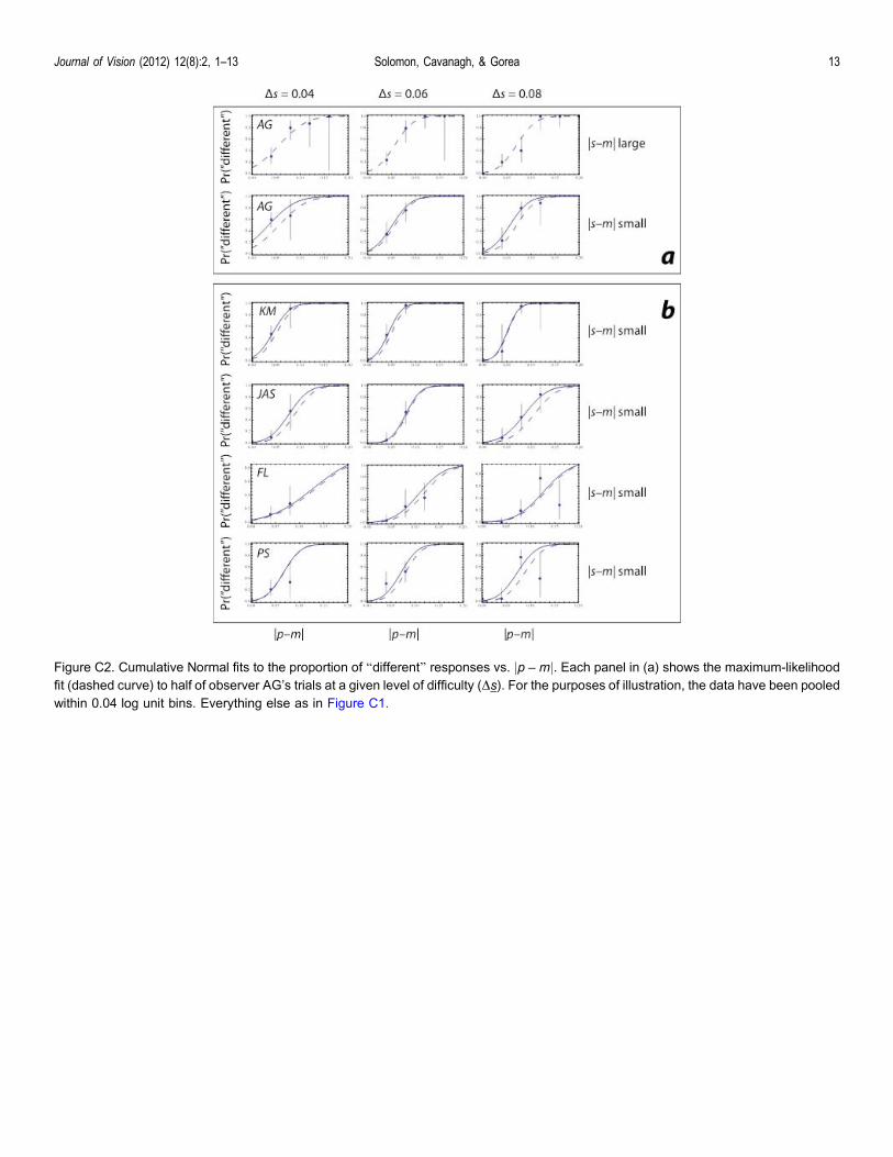
Figure C2. Cumulative Normal fits to the proportion of ‘‘different’’ responses vs. jp – mj. Each panel in (a) shows the maximum-likelihood

fit (dashed curve) to half of observer AG’s trials at a given level of difficulty (Ds). For the purposes of illustration, the data have been pooled

within 0.04 log unit bins. Everything else as in Figure C1.

Journal of Vision (2012) 12(8):2, 1–13 Solomon, Cavanagh, & Gorea 13