Optimal Compulsion when Behavioral Biases Vary and the State Errs

Salvador Valdés-Prieto Ursula Schwarzhaupt

CESIFO WORKING PAPER NO. 3316 CATEGORY 1: PUBLIC FINANCE

JANUARY 2011

An electronic version of the paper may be downloaded • from the SSRN website: www.SSRN.com • from the RePEc website: www.RePEc.org

• from the CESifo website: Twww.CESifo-group.org/wp T

CESifo Working Paper No. 3316

Optimal Compulsion when Behavioral Biases Vary and the State Errs

Abstract When behavioral biases have varying sizes, and the State seeks to correct behavior through compulsion, the question is how to design optimal compulsion. One argument is that the amount of compulsion should rise with the size of the bias to be “cured”. A contrary argument is that since compulsion affects actions, and recommended actions are independent from the bias, the amount of compulsion should not depend on the bias. This puzzle is solved for the case where individuals are affected by a bias that leads them to under-save, acknowledging that the planner predicts each individual’s optimal action with error. Since only low-bias individuals are able to correct the planner’s mistakes when mandated to save too little, but not in the opposite direction due to a costly spread, the optimal amount of compulsion rises with the predicted bias. As an application, the paper explores a behavioral rationale for a Maximum for Taxable Earnings (MTE). It finds that if (1) the State’s information is limited to current earnings; (2) earnings do not influence the earnings ratio for old age; and (3) the bias is smaller only for the highest earnings quintile, then a MTE near the 80th percentile of the earnings distribution is optimal.

JEL-Code: H550, H530, H240.

Keywords: behavioral bias, compulsion, optimal policy, time-inconsistency, overoptimism, pensions, maximum taxable earnings.

Salvador Valdés-Prieto

Economic Institute Pontificia Catholic University of Chile

svaldes@hacienda.cl

Ursula Schwarzhaupt Central Bank of Chile

uschwarzhaupt@gmail.com

First draft: January 13, 2010 This version: January 3, 2011 We appreciate comments from participants at seminars at the CESifo Area Conference on Employment and Social Protection, May 14-15, 2010, at the annual meeting of Chilean Economists in September 2010 and at Catholic University of Chile (Santiago) in March 2010 were useful for this paper.

- 2 -

1. Introduction Many heavy smokers, drinkers and spenders regret their behavior later on, when there is no free turnaround to recover what has been lost. Since these biases affect different individuals to different degrees, and the “correct” behavior is difficult to predict, public policies aimed to correct such biased behaviors can do more harm than good, for many or even for most individuals. But laissez-faire may also do worse than a modest amount of simple compulsion. The question tackled in this paper is how should a benevolent planner vary the amount of compulsion, taking into account his own errors, both when estimating each person’s optimal action and when assessing the size of the bias for each individual. A natural rule of thumb is that compulsion should be targeted to those with large behavioral biases, and that others should be exempt (Gill et al 2005). Indeed, Saint-Paul (2009) asserts that since behavioral biases are essentially a matter of the poor, compulsion should be targeted to the poor alone. However, this rule-of-thumb is not straight-forward. A benevolent planner would try to reach the optimal action for the individual in the absence of bias. Thus, the optimal action would not depend on each individual’s level of bias, precisely because the bias is what needs to be set aside. If the planner can adjust the individual’s behavior by making the optimal action compulsory, it follows that the amount of compulsion should not depend on the level of bias. This paper proceeds in two steps. First, it identifies conditions under which the optimal amount of compulsion is independent from the level of bias. The critical condition turns out to be that the planner is able to predict accurately each individual’s optimal action. In that setting the planner’s other mistake, concerning the assessment of each individual’s bias, does not matter. Second, the paper identifies optimal policy in the realistic case where the planner errs in assessing each individual’s optimal action. These mistakes make compulsion less efficient, creating scope for voluntary action. Indeed, Beveridge argued that “the State in organizing security should (…) leave room and encouragement for voluntary action by each individual to provide more than that minimum for himself and his family” (Beveridge, 1942, p. 7).1 In this paper free action (no compulsion, or laissez-faire) is valued instrumentally, as the means for avoiding the inefficiencies created by the planner’s mistakes.

For incomplete information scenarios, the optimal level of compulsion does depend on the predicted bias for each individual. Let us illustrate with an example, where a planner seeks to increase saving for old age because a behavioral bias leads many to save less than optimal. On average, the planner knows that he might mistakenly force some individuals to oversave, while others might be required to save too little relative to their bias-free needs. When compulsion is set higher than what the individual deems optimal, the individual does not counteract over-saving if the cost of consumer credit is prohibitive. In contrast, when the mandatory saving rate is set below what the biased individual would have chosen freely, the individual can respond in two ways: if her bias is small, she can be relied upon to repair most of the planner’s mistake by raising her voluntary savings. However, if her bias is large, she will not repair the mistake and will indulge in her biased behavior.

1 The literature on why a wider scope for free action is desirable includes Regan (1983) and Zamir (1998). On paternalism and the value of individual freedom, see also Burrows (1993) and Buchanan (1959).

- 3 -

Therefore, the planner’s cost of under-predicting the optimal mandatory saving rate is larger when the individual’s bias is larger. In contrast, the cost of mandating the individual to oversave is independent from the size of the bias that affects each individual. This asymmetry leads the optimizing planner to cut the compulsory contribution rate for individuals whose bias is predicted to be low. Thus, the optimal amount of compulsion should rise with the bias.

This rationale fades as the planner predicts the optimal action more accurately. The precision of the predicted bias is important too. As this precision falls, the conditioning of compulsion on the predicted level of bias is reduced gradually under optimal policy, and is eventually eliminated. The last part of this paper applies these general results to a long-standing issue in pension economics. Imagine that higher earnings are correlated with a smaller bias regarding old-age savings, and therefore high earners are less affected by insufficient compulsory saving. The previous results suggest that it would be optimal to reduce the compulsory contribution rate on high earners. This might support a “behavioral rationale” for the well-known policy that sets a maximum on taxable earnings (MTE). Table 1 reports the MTE for a sample of 60 countries in 2008, expressed as a ratio of GDP per capita. The observed ratios are diverse: nearly a fifth of the countries set a MTE below their own GDP per capita; a fifth go to the opposite extreme and set no limit at all. The middle 60% exhibits a median MTE equal to 2.26 times GDP per capita. This ratio is 2.33 for the U.S.A. About 83% of the sample with a finite MTE reduces the marginal contribution rate by at least 75% as the MTE is surpassed. The size of the MTE is at the crux of an old debate between the Beveridgian and the Bismarckian designs for contributory old-age pensions that are not redistributive. Beveridge’s (1942) prescription was a contributory system of flat old-age benefits financed with a flat amount of contributions per worker.2 This implies a MTE equal to the minimum wage, at the lower end of the feasible range for MTEs. In contrast, Bismarck’s (1889) prescription was a single contribution rate applied to all earners, which implies an unbounded MTE. When the MTE is set at a mid-point, its size tells the degree of “Bismarckianess” of the pensions system. Demand for mid-point MTEs runs strong among modern policymakers. For example, the 2004 Report of the UK Pension Commission posited that “there is a social interest in ensuring that people of modest or average means (e.g. those up to the 75th percentile of earnings) have made provision which they would consider adequate, but that above some level of income (say above the 90th percentile) a purely individualist approach is appropriate.” (Report, p. 129) 3.  How does this paper contribute to this debate? First, a disclaimer: there are at least three main benevolent rationales to adopt or change a MTE: fiscal, market-structure, and behavioral. 4

2 Not to be confused with systems where a proportional tax on earnings finances a flat benefit for the old. Such a redistributive and non-contributory system was mistakenly labeled as “Beveridgean” by Cremer et al (2007). 3 This Report is available at www.pensionscommission.org.uk 4 Gill, Packard and Yermo (2005, p. 230-232) contribute two other benevolent rationales in support of a MTE. First, they posit that personal investments such as owner-occupied housing and prepayment of expensive consumer credit, provide higher returns than the purchase of pension rights even under full funding. Second, they argue that for low earners compulsion is not costly, because high-return personal investments are denied to them anyway by non-divisibility thresholds. If less compulsion allowed some high earners to accumulate enough savings to overcome those thresholds, the opportunity cost of compulsion would be larger for high than for low earners.

- 4 -

Fiscal and market-structure rationales for a MTE are outlined in section 6.2. This paper’s contribution to this debate relates only to behavioral rationales for a MTE. There is empirical backing for the hypothesis that high earners have a lower bias on average. For example, Stango and Zinman use the 1983 Survey of Consumer Finances in the U.S.A. to measure “exponential growth bias” and find that its size is significantly lower for the highest earnings quintile (2009, Table IV). We have found no empirical evidence on the link between earnings in the first phase of life and net earnings in old age. This paper fails to support in general the behavioral argument for a finite MTE. A modern State observes each individual’s current taxable earnings, age, occupation, rural/urban status, education, marital status, wealth, gender and other socio-demographic attributes. Let us assume that anti-discrimination legislation does not preclude a State from conditioning the compulsory contribution rate on at least one of the attributes with impact, apart from earnings. For example, in Switzerland the mandatory contribution rate for old age-savings depends on age, and in many countries it also depends on occupational sector and on labor market status. Therefore, conditioning the amount of compulsion on current earnings alone is inefficient. Recently, Stango and Zinman (2009, Table IV) found that the size of “exponential growth bias” is strongly influenced by education, after controlling for the impact of the current earnings quintile and gender. Thus, the Beveridgian and the Bismarckian extremes, and also intermediate levels for the MTE, make suboptimal use of information. Next, the paper explores optimal policy for an informationally constrained State, who is limited to observe current earnings. If the current earnings quintile is the only predictor of both the bias and net earnings in old age for an individual, the paper finds that optimal policy still depends on the impact of earnings on the optimal age-earnings ratio for old age. For example, if a higher salary induces earlier retirement by enough, it reduces the overall earnings obtained in the second phase of life, and this increases desired savings for old age. If this link is important, it influences the optimal schedule that connects the contribution rate and current earnings. Indeed, a strong impact of this type may convert the optimal MTE into a Lower Earnings Limit. Therefore, an MTE may be suboptimal even for a State subject to this informational limitation. However, in the further subcase where earnings have a negligible influence on the desired age-earnings ratio for old age, the inability to observe data other than current earnings brings the MTE approach close to optimality. For example, if the bias is flat for most earnings quintiles, except for the highest, where the bias falls, as in the data for the U.S.A., then informational limitations make an MTE optimal near the 80th percentile of the earnings distribution. For the Beveridgean system to be optimal, the predicted bias needs to fall continuously as earnings rise above the minimum salary. For the Bismarckian system to be optimal, all workers need to be equally biased, including those in the highest earnings quintile. Both are rejected for U.S.A. data. Section 2 reviews briefly the literature on benevolent compulsion. Section 3 presents a simple model of excessive optimism, the behavioral bias used in this paper. Section 4 explores the case of a planner whose informational resources allow accurate prediction of the optimal action. Section 5 defines and simulates optimal policy for States with realistic amounts of informational resources, and obtains the main results. Section 6 discusses application to the optimal Maximum Taxable Earnings in old-age pensions policy. Section 7 suggests directions for future research.

- 5 -

2. Brief review of the literature on benevolent compulsion in saving for old age

Altruism leads people to vote for policies that alleviate poverty. However, then some of the young that have modest earnings may engage in under-saving to benefit from subsidies to the old-age poor. Compulsion has been justified as a policy that prevents this response (Hayek 1960 p. 286, Musgrave 1968, Kotlikoff 1987). This argument is also referred to as the “savings moral hazard” or “rational prodigality” hypothesis. However, recent literature has shown that when a negative income tax is available, the State should never use compulsion, because compulsion deepens distortions to the labor choices of the young poor , who prefer to work less to avoid compulsory savings (Homburg, 2006). If compulsory savings drives consumption of the young poor that work too close to subsistence, voters would not be altruistic (Valdés-Prieto, 2000).

Time-inconsistency is a more robust argument for compulsion. Several branches of time-inconsistency theory are relevant for old-age saving. The “hyperbolic discounting”, “finite horizons” and “procrastination” branches stress that people have great concern for immediate consumption, but neglect distant consumption, and this leads them to under-save. The difference between these branches lies in the way they model preference for future consumption. Under “hyperbolic discounting”, the discount factor falls steeply at first and then flattens out. (Laibson 1997, Imrohoroglu et al 2003, Fehr et al 2008). In the “finite horizon” branch, the discount factor is constant for several periods up to some moving horizon, beyond which it drops abruptly to zero (Feldstein 1985, Docquier 2002, Caliendo and Aadland 2007). In “procrastination” models, hyperbolic discounting is supplemented by a second aspect of preferences: the individual is hopeful (naively) that her own degree of hyperbolic discounting will diminish in the future (O'Donoghue and Rabin, 2001).

A fourth branch of time-inconsistency is “unrealistic optimism” (Weinstein1980, Scheier, Carver and Bridges 1994), also referred to as “overconfidence” (Malmendier and Tate 2005, Caliendo and Huang 2008) in the finance literature. In this case, individuals suffer from an optimistic bias when projecting their future budget sets, not their future preferences. This bias can take several forms. Expenses at old age, such as health costs, may be projected to be lower than unbiased estimates. The young may anticipate higher earnings when old than they should. Evidence in favor of unrealistic optimism has been offered by Quadrel et al (1993), Weinstein and Klein (1996), and Puri and Robinson (2007). In Germany the SAVE survey found a large bias in expected lifetime: women aged 35-75 underestimate their life by about five years, while men aged 35-70 do so by about four years (Steffen 2009, fig. 4.6). The model presented below belongs to this branch of time-inconsistency. Finally let us review the empirical backing for the hypothesis that high earners have a lower bias on average. This backing may be different for each specific model for the bias. Stango and Zinman (2009) use the 1983 Survey of Consumer Finances to measure “exponential growth bias” and find its size is negatively correlated with current earnings. Bhandari and Deaves (2006) use survey evidence for 2,000 Canadian employees to measure another bias, defined as the difference between knowledge perception and actual knowledge, and find it is weakly positively correlated with current earnings (Table 3). Puri and Robinson (2007) define “extreme optimism” as belonging to the right-most 5% of individuals in the distribution of differences between self-reported life expectancy and that implied by statistical tables. They find that

- 6 -

“extreme” optimists have short planning horizons and save less than “moderate optimists”, who display prudent financial habits. They do not report the demographics of extreme optimists.

3. A simple behavioral model for compulsory contributions

We use a model in which individuals are affected by an overconfidence bias, which a benevolent planner tries to correct. In this model individuals may limit the effects of compulsion by reducing voluntary savings, and also by accruing expensive consumer debt.

3.1 The labor market

The life cycle is collapsed into two separate periods, the active phase and old age. Each period lasts 30 years with active age beginning at age 20, and old age at age 50. Define:

ya = net earnings in the active phase. yp

e = expected net earnings in old age. It is net from health expenses in old age. ψ e≡ yp

e /ya = net old-age earnings ratio, as expected by the individual in her active phase. To

simplify, this paper assumes that individuals believe they have a fully accurate estimate of ψ e. The supply of hours of labor at each age is set institutionally, so it is inelastic to wages. The model focuses on the impact of a behavioral bias. Define: ψ = unbiased net old-age earnings ratio when old. b ≡ ψ e−ψ = size of the behavioral bias suffered by this particular individual. If ψ e> ψ , the individual suffers an overconfidence bias. Note that the bias b is defined as a proportion of net earnings in the active phase. Ageing is represented by ψ e < 1 and ψ < 1.

3.2 The contributory old-age pensions system The compulsory pensions system is described by two formulae: one for benefits and another for the contribution amount. The average contribution rate for any given individual is

aa yyC /)(≡θ , where C(ya) is the contribution amount when reported earnings is ya.

Other branches of social insurance, such as health insurance and unemployment insurance, usually create an extra tax on covered earnings because the marginal benefit from extra contributions is smaller than the marginal contribution, in expected present value. Define: ta = net tax rate on covered earnings levied by other branches social insurance. This tax is net

from any marginal benefits supplied directly by those branches to the individual. Turn now to the pension benefit formula. Define:

ρc = internal rate of return paid by the contributory pensions system to each generation of participants. This rate governs the link between individual benefits and contributions.

- 7 -

With two-period lives, the amount of the pension benefit is simply the contribution times the gross rate of return, or ( )cay ρθ +⋅⋅ 1)( . It is further assumed that the compulsory pensions system is fully funded (see reasons in section 6.2). This implies:

(1) PFPFc rr =−⋅= )1( τρ

where r is the pre-tax rate of return paid out in the capital market, and τPF is the tax rate levied on the capital income of the pension fund (interest, dividends and net capital gains)5. The model is partial equilibrium because r is fixed, or applies to a small open economy.

3.3 The individual’s budget constraint To obtain each period’s budget constraint, define: F = stock of voluntary financial savings at the end of the active phase.

r = pre-tax rate of interest paid on voluntary (financial) savings (F >0).

τS = tax rate levied on the return from voluntary saving. )1()( Srr τ−⋅≡+ = after-tax rate of interest paid to voluntary saving deposits (F >0).

srr ++≡− )()( = rate of interest paid on consumer loans (F < 0), with s being the net interest spread6. Positive administrative and marketing costs in financial intermediation, and a positive gross interest rate r, guarantee that s > 0. A positive spread creates a kink in the budget constraint that limits the range where perfect substitution between compulsory and voluntary saving applies. Because of the positive spread, a number of individuals choose not to use consumer credit to undo mandatory contributions. This kink in the budget constraint limits consumer credit, but does not limit saving, an asymmetry that turns out to be important for optimal compulsion. The period budget constraints perceived when young are: (2a) Ftyc aaa −−−⋅= )1( θ (2b) )](1[)1( FnrFryyc PFaa

ep +⋅++⋅⋅+⋅= θψ

where nr(F) = r(-) if F ≥ 0 and nr(F) = r(+) if F < 0. For simplicity, it is assumed that rPF = )1()( Srr τ−⋅≡+ . This applies, for example, under fully-funded pension finance and equal tax treatment for voluntary and compulsory saving for old age.

3.4 Individual optimization in the active phase

The individual maximizes lifetime utility, which is assumed to be additively separable across phases of life. The individual solves the following standard problem (P1) in the active phase:

5 The tax rate τPF should be interpreted as the sum of the personal income tax rate with the portion of the corporate tax rate that cannot be deducted from personal taxes (Feldstein and Liebman 2002). 6 The authorities add interest income to the taxable base, but do not allow interest paid in loans to be deducted from the taxable income. In addition, fiscal incentives for voluntary saving for old age channeled through the financial market are not affected in any way by interest paid in consumer loans.

- 8 -

{ }

( ))](1[)1()(

1)(

)()(

FnrFryycB

FtycA

tosubject

cucuUMax

PFaae

p

aaa

paF

+⋅++⋅⋅+⋅=

−−−⋅=

⋅+≡

θψ

θ

β

where u’ > 0, u’’< 0.

The choice of F* is standard, determined by preferences (discount factor β and intertemporal elasticity of substitution σ), by the spread s that governs the net return nr(F), and by the distribution of earnings in the life cycle perceived by the individual, given by her own perceived net old-age earnings ratio ψe. Note that the planner’s unbiased estimate of productivity ratio when old, defined as ψp, does not influence voluntary saving F*. This discrepancy is the basis for benevolent policy.

4. Optimal compulsion in extreme informational scenarios This and the next section show that the planner’s choice of optimal compulsion depends critically on the information he possesses about the individual’s preferences and opportunities. The planner’s optimal contribution rate is identified in three scenarios, which differ by the amount of information the planner has. In all scenarios, the planner is supposed to know ta, r and τS because they are common to all individuals, and to know θ because it is set by himself. 4.1 Optimal compulsion for third-best information

The scenario designated here as “third-best” is the one where the planner has the least information. The planner does not have information about each individual´s personal circumstances, parametrized in section 3 by ψe, s, β and σ. Imagine that the planner suspects that there is a correlation between personalized earnings ya and the individual’s degree of overconfidence b (as posited by Saint-Paul, 2009). However, assume also that personalized earnings ya are not observed by the authorities. For example, this occurs when employers do not break down contributions by worker, say because of the lack of a national identification number, or because of costly or inefficient administration. Thus, in a third-best scenario the planner is ignorant of each individual’s degree of overconfidence b. In such a case the compulsory contribution formula must be uniform.7 There are two uniform options, and its combinations. One is a flat compulsory contribution amount per employed person (Beveridge), and the other is a single contribution rate that applies to the full payroll (Bismarck). However, a Beveridgean flat contribution is free from evasion, and thus viable, only if the authorities can observe personnel movements and hours hired to each employee. If not, a flat contribution would allow employers to minimize contributions by underreporting the number of employees. Even when the planner observes the number of workers, but there is a minimum number of hours of work that must be met before a worker causes a compulsory contribution, employers can evade by underreporting the number of their employees that work hours above 7 There is no scope for a finite MTE, because lifetime personalized earnings ya are not observed by the authorities.

- 9 -

the threshold. It is precisely in the third-best informational setting where the planner is unlikely to have access to information about personnel movements and hours worked by each employee. If the set of employers free to underreport is large enough, the only feasible design is Bismarckian.8 This immediately establishes the following: PROPOSITION 1: With third-best information, the only feasible MTE is indefinitely large, as in the Bismarckian design. The only remaining issue is how to determine the size of the Birmarckian contribution rate θ. In this scenario the planner may still use surveys, or other means, to determine the joint distribution of the unbiased old-age net earnings ratioψ in the population and the degree of overconfidence b, together with other personal preferences and circumstances information, which can be summarized in density h(ψe, b, s, β ,σ).

A best “one size fits all” contribution rate takes into account that the planner is averse to the risk that insufficient compulsion cuts unbiased welfare. He is also averse to the risk that excessive compulsion reduces welfare, especially below laissez-faire levels, which is a possibility illustrated in section 4.2. The planner’s aversion to these outcomes is represented by a constant relative risk aversion function with parameter η ≥0. As the coefficient η rises, the planner cares more about the utility losses caused. Consequently, the planner should choose θ by maximizing:

(3) [ ]

)1(),(

),,,,(1

1)()()(

PArgMaxcctosubject

ddbdsddsbhcucu

W

ba

eepau

=

⋅−

−⋅+≡ ∫ σβψσβψ

η

ηβθ

4.2 Optimal compulsion for first-best information The “first-best” informational scenario is defined as one where the planner has access to very detailed information about each individual, that allows a very accurate estimate of the unbiased net earnings ratio when old for each individual (ψ). Specifically, in this scenario the planner knows preference parameters such as the utility discount factor β and the elasticity of intertemporal substitution σ, and knows the spread s on each individual’s consumer credit (and in a more general model, the return of private investment opportunities). The planner also observes active life earnings, ya. It will be shown that accurate estimation of the bias b is not important in the first-best scenario. 4.2.a The first-best personalized contribution rate The benevolent planner solves P1 using his realistic, unbiased estimate for the individuals’s productivity ratio when old, ψp. The planner seeks to correct the bias by forcing the individual to save what her unbiased self would have liked. Nevertheless, he is aware that the individual can react to the mandate by reducing voluntary savings, which he cannot control. 8 This informational scenario also has implications for the benefit formula. If the authorities have administrative resources that at most allow observation of earnings in the last few years before the pension starts, then only a years-of-service formula based on the last few earnings is feasible, along with flat benefits. This informational setting is incompatible with an actuarial benefit formula based on lifetime contributions or lifetime earnings.

- 10 -

In this informational scenario, the planner’s decision can be modeled as in Valdés-Prieto (2002). The planner maximizes the individual’s unbiased welfare, Wu, subject to her budget constraint and to her response in terms of voluntary saving (the solution to P1). The planner solves the following problem (P2), separately for each individual:

{ }

{ }{ }

)](1[)1()2(

)1()1(

)()()(

)](1[)1()(

)1()(

)()()(

FnrFryycC

FtycC

tosubjectcucuMaxArgFC

FnrFryycB

FtycA

wherecucuWMax

PFaaebiased

p

aabiaseda

biasedp

biasedaF

biased

biasedbiasedPFaa

pp

biasedaaa

pau

+⋅++⋅⋅+⋅=

−−−⋅=

⋅+=

+⋅++⋅⋅+⋅=

−−−⋅=

⋅+≡

θψ

θ

β

θψ

θ

βθθ

Note that lines (B) and (C2) use different assessments for the net productivity ratio when old. The planner’s unbiased ψe in (B) reflects the ability of the authority to exactly predict earnings when old. In contrast, (C2) uses the biased ratio ψe ( ≡ ψp + b) because the individual chooses voluntary saving by relying on her own (biased) assessment of net productivity ratio when old. b is a ratio, hence may be called a “proportional” bias. Note that b is predicted with full accuracy in (P2). From (B) and (C2) and from F = Fbiased from (C) it follows that: (4) ( ) aa

pep

biasedp ybycc ⋅≡⋅−=− ψψ Thus, if b > 0, then cp < cp

biased.

This confirms that an overconfident individual plans to consume more when old than she will actually consume9. The planner predicts this surprise and adjusts θ to help the improvident. Figure 1 describes the planner’s problem in the first-best scenario, by reporting the amount of voluntary saving chosen by an individual, as a function of the compulsory contribution rate θ. The figure is obtained with the parameter assumptions in the Appendix, for a specific value of the bias b of 0.20 (old age earnings is over predicted by 20% of active age earnings).

Figure 1 shows that at low contribution rates, voluntary saving is substituted perfectly for mandatory saving. This is a standard result, because in this model, the link between contributions and benefits is the same in both types of saving. In this illustration, voluntary assets fall to zero when the contribution rate comes close to 16%. For higher contributions rates, total saving rises. For contribution rates above a number close to 36% in the illustration, total saving rises more slowly, because the individual chooses to leave the corner with F = 0 and takes some consumer

Figure 1: Voluntary, Compulsory and Total Saving in response to θ, first-best

9 In a simple two-period life model, this negative income shock is perceived just at the end of her active phase. However, with a more realistic number of periods, the shock would be spread out over different ages.

- 11 -

credit, which carries the obligation to pay the spread s. Since this spread reduces wealth, substitution between compulsory saving and consumer debt is imperfect. Although this simulation assumes that the spread s is merely 10% per annum (it is much larger in many emerging countries), it still creates a very wide range of contribution rates where voluntary saving is zero. In this illustration this range is about 20 percentage points wide. 4.2.b How the bias affects the first-best amount of compulsion

This subsection analyzes the hypothesis that the optimal amount of compulsion becomes smaller as the estimated bias b for the individual decreases (Gill et al 2005, Saint-Paul 2009).

As shown by (P2), the planner needs to estimate each individual’s bias. Assume that the planner does observe a number of individual attributes, say because a personal identification number for workers allows employers to report personalized contributions and administration of personalized records is efficient enough. The planner may invest in surveys to estimate the relationship between each individual’s degree of overconfidence (the bias b) and her earnings ya and other attributes za such as age, gender, residence area, type of job, etc.. Through this method or others, the planner comes to learn the following relation that predicts each individual’s bias: (5) .0)(;0)(;),( =>+= εεε EVarzyBb aa

where b is the actual bias and B(ya,za) is the predicted bias for an individual with earnings ya and other attributes za.10 The error term ε summarizes the impact of variation across individuals in (ψe , s, β, σ) within the subset that shares a common set of observable variables (ya,za), and Var(ε) measures one aspect of the planner’s ignorance.

10 Saint-Paul (2009) suggests that ∂Β/∂ya < 0.

- 12 -

The case of zero variance for ε is analyzed first. Figure 2 shows unbiased individual welfare for different levels of the actual and predicted bias (these coincide for Var(ε) = 0, as shown by (5)). For a zero bias (b = 0, Var(ε) = 0), the level of unbiased welfare is represented by the higher dashed lines. In this case compulsion is irrelevant as long as the contribution rate θ is below the voluntary saving rate in the absence of compulsion. In the case of zero bias, the first-best amount of compulsion is not unique, because there is perfect substitution between voluntary and compulsory saving in the fiscally neutral setting analyzed in this paper. In this case it is incorrect to assert that the only best policy is no compulsion (θ* = 0).11 For a positive bias (b > 0), and Var(ε) = 0, Figure 2 shows that a well-chosen compulsory rate raises unbiased welfare above the level attained in laissez-faire, which is the level attained when the compulsory contribution rate is zero. It also shows that when the compulsory contribution becomes large enough, the individual is forced to save “too much” in the sense that her unbiased welfare falls steeply. Since unbiased welfare can fall below the laissez-faire level, the range of contribution rates in which benevolent first-best social insurance is justified is finite.12

Figure 2: Unbiased Welfare versus contribution rate for different actual biases

Three lessons follow from figure 2. First, compulsion does not improve unbiased welfare if the contribution rate is small enough, due to perfect substitution of compulsory for voluntary actions. Second, the size of the actual bias affects the size of the smallest contribution rate at which unbiased welfare can be improved by compulsion. This “smallest effective contribution rate” is inversely proportional to the actual degree of overconfidence b, because the size of actual b or ψe influences the individual’s decision. Third, for contribution rates above the

11 The same result obtains for cases with b < 0 (unjustified pessimism, leading to oversaving). Since compulsory saving is unable to help the individual, these cases are represented in Figure 2 by the line for b = 0. She chooses some point in the right-hand side of the curve. Her unbiased welfare falls as her degree of pessimism rises. 12 For very large contribution rates, where the individual responds by issuing consumer debt, the negative wealth effect caused by the cost of spread s creates a kink in the curve in Figure 2, in the rightmost range.

- 13 -

“smallest effective contribution rate”, the size of the actual bias does not influence the individual’s decision (the amount of voluntary saving F*), because it is already at a corner, and thus is fixed (at zero in this model). Most important, optimal compulsion θ is independent from the size of the actual bias. Figure 2 shows clearly that the size of the actual bias b does not affect the planner’s decision in this informational scenario. It follows that the predicted bias B, and thus (ya,za) are irrelevant for policy. The intuition is that the planner’s optimal compulsion is always equal to the voluntary saving rate in the absence of bias, regardless of the size of the actual bias. Of course, this result obtains only because the planner never errs in determining the individual’s optimal total saving in the absence of bias. This is what first-best information is about, i.e. planner knowledge of each individual’s true (ψ, s, β, σ). These results extend also to the general case with Var(ε) > 0. In this case the three cases shown in Figure 2 can be interpreted as consequences of three different values for ε. Since the optimal θ is the same for all values for ε, and the planner maximizes a weighted average of the unbiased individual welfares that result for each value for ε, it follows that the optimal θ is the same for any distribution of ε. One corollary is that the size of error ε, and of Var(ε) are irrelevant for policy, i.e. for the optimal θ. Again, this result obtains because the planner does not err when determining the individual’s optimal total saving in the absence of bias. Summarizing, PROPOSITION 2: With first-best information regarding optimal actions, and in the absence of fiscal consequences, a) The hypothesis that the optimal amount of compulsion for an individual is smaller when her actual or predicted bias is smaller, is false. b) The optimal personalized contribution rate is independent from each individual’s bias, and errors in estimating these biases are irrelevant for policy.

5. Optimal compulsion for intermediate informational scenarios

The “second-best” informational scenario is defined here by an intermediate degree of information asymmetry faced by the planner regarding his unbiased estimate of the bias-free saving rate, determined at least by the net earnings ratio when old for each individual (ψ). His informational resources do not allow him to know exactly the values of (ψ, s, β, σ) for each individual, To model this realistic case, define:

(6) .0)(;0)(;),( =>+= δδδψψ EVarzy aa

p

where ψ is the actual old-age net earnings ratio, ψp is the old-age net earnings ratio predicted by the planner using the information available and δ is the planner’s error in predicting the old-age net earnings ratio.

Since the planner also predicts the bias b with error (recall equation (5)), the issue to be explored is how optimal policy varies in response to different values of the two types of planner mistakes, measured by Var(δ) and Var(ε).

- 14 -

5.1 The second-best contribution rate for Var(ε) = 0. In this informational scenario, the planner faces significant uncertainty about the value of the individual’s old-age net earnings ratio, but predicts her bias accurately.

A positive error δ > 0 leads the planner to underpredict net earnings in old age (note that δψψ −=p ), and in turn overpredict the voluntary savings F* desired by the individual for old

age. Therefore, for δ > 0 the naive planner would impose a compulsory contribution rate θ that is above her optimum. Conversely, a negative error δ < 0 leads the planner to impose a contribution rate that is lower than optimal.

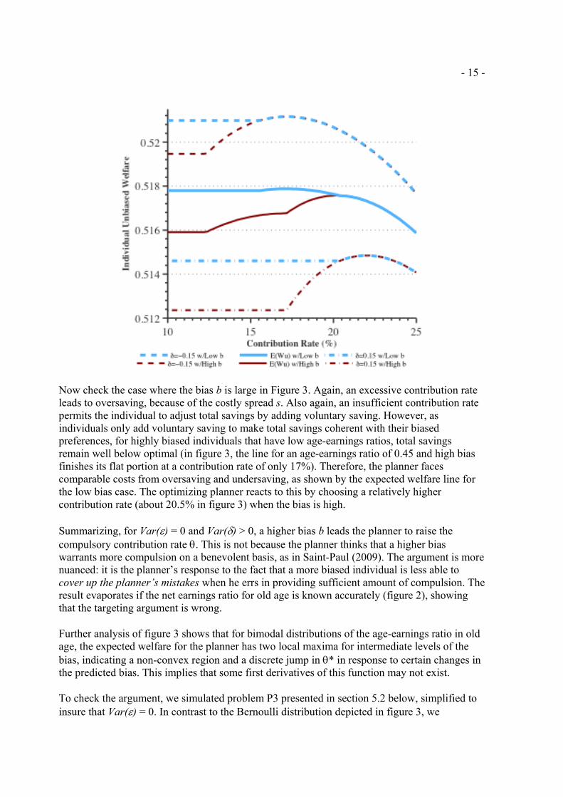
Figure 3 illustrates the case where δ follows a bimodal distribution, with values 0.15 or -0.15 with probability 0.5. The planner predicts a central value for ψ equal to 0.6, but knows the actual value could be either 0.75 or 0.45. Lighter lines show the case for low bias (b = 0.1), whereas the darker lines show higher bias (b = 0.3), with no planner mistakes in predicting the bias. The higher dashed lines represent the lifetime welfare the individual would face when the planner underpredicts ψ; similarly, the dash-dotted lines represent the individual lifetime welfare when the planner overpredicts ψ. The middle lines show expected welfare as seen by the planner. He simply averages the vertical values of welfare, for each value of θ. In the Bernoulli distribution depicted, expected welfare for low values of θ is simply welfare for the high value of the old-age earnings ratio multiplied by 0.5 plus a constant. This constant reflects the fact that in response to low contributions, the individual with low old-age earnings ratio raises her voluntary savings to achieve the same total amount of savings, and the same welfare, that would have prevailed under laissez-faire.

When the bias b is known to be small, the mistakes made by the planner when predicting ψ have asymmetric impacts: an excessive contribution rate imposes higher expected costs than an insufficient one. An excessive contribution rate leads to oversaving, because given the costly spread s, the individual prefers not to adjust by issuing consumer debt. Thus, excessive compulsory contributions reduce welfare. On the other side, because the bias b is small, the amount of total saving is close to optimal. Therefore, it is best for the planner to err from below than from above, when setting the contribution rate for a low-bias individual. This is clear in figure 3, in the light lines corresponding to low bias. It can be seen that the planner would impose considerable damage by setting a high contribution rate (above 17.5% in the figure) if he had underpredicted ψ, whereas the individual would be little affected by a low contribution rate if the planner had overpredicted ψ. The highest expected welfare seen by the planner is reached at a relatively low contribution rate. Indeed, it is reached exactly at the same contribution rate that would have prevailed if the planner had known accurately the net earnings ratio in old age of the low-bias individual and had ignored the case of high net earnings ratio. Figure 3: Optimal policy based on low-bias individuals’ corrections to the planner's mistakes

(Welfare and expected welfare when δ is bimodal and the bias varies)

- 15 -

Now check the case where the bias b is large in Figure 3. Again, an excessive contribution rate leads to oversaving, because of the costly spread s. Also again, an insufficient contribution rate permits the individual to adjust total savings by adding voluntary saving. However, as individuals only add voluntary saving to make total savings coherent with their biased preferences, for highly biased individuals that have low age-earnings ratios, total savings remain well below optimal (in figure 3, the line for an age-earnings ratio of 0.45 and high bias finishes its flat portion at a contribution rate of only 17%). Therefore, the planner faces comparable costs from oversaving and undersaving, as shown by the expected welfare line for the low bias case. The optimizing planner reacts to this by choosing a relatively higher contribution rate (about 20.5% in figure 3) when the bias is high.

Summarizing, for Var(ε) = 0 and Var(δ) > 0, a higher bias b leads the planner to raise the compulsory contribution rate θ. This is not because the planner thinks that a higher bias warrants more compulsion on a benevolent basis, as in Saint-Paul (2009). The argument is more nuanced: it is the planner’s response to the fact that a more biased individual is less able to cover up the planner’s mistakes when he errs in providing sufficient amount of compulsion. The result evaporates if the net earnings ratio for old age is known accurately (figure 2), showing that the targeting argument is wrong.

Further analysis of figure 3 shows that for bimodal distributions of the age-earnings ratio in old age, the expected welfare for the planner has two local maxima for intermediate levels of the bias, indicating a non-convex region and a discrete jump in θ* in response to certain changes in the predicted bias. This implies that some first derivatives of this function may not exist.

To check the argument, we simulated problem P3 presented in section 5.2 below, simplified to insure that Var(ε) = 0. In contrast to the Bernoulli distribution depicted in figure 3, we

- 16 -

generated 200 values for δ taken from a uniform distribution. We then created 200 identical individuals differing only in their assigned δ, and optimized θ for several known values for the bias b. To avoid results from being influenced by the particular sample of δ, we repeated this experiment 100 times for each value of bias b, and averaged the optimal θs 13. An important result (not shown) is that expected welfare has a single local optimum for θ in this stochastic setting, for all values of b and Var(δ). This result suggests that unless the distribution of δ exhibits abrupt jumps, as for figure 3, non-convex regions do not exist and standard comparative statics can be applied. Table 2 presents the results of these simulations. Table No. 2 : Optimal compulsory contribution as function of a bias that is accurately predicted

(Var(ε) = 0; The planner’s prediction about the old-age net earnings ratio is ψp = 0.60 and the error in this prediction is δ ~ U(–D,D) with variance is D2/3)

Optimal θ Predicted bias B

( =b, Var(ε) = 0) Var(δ) = (0.1)2/3 Var(δ) = (0.2)2/3 0.001 0.1800 0.1632 0.05 0.1883 0.1707 0.10 0.1967 0.1818 0.15 0.1968 0.1933 0.20 0.1968 0.1995 0.25 0.1968 0.1995 0.30 0.1968 0.1995 0.40 0.1968 0.1995

Source: Authors’ simulations based on P3 and parameters in the Appendix.

Table 2 reveals that optimal compulsion indeed rises with the bias. This is because the planner takes advantage of the fact that the less biased individual does better in covering up his mistakes. Table 2 shows also that when the planner is more uncertain about his own knowledge about the optimal action, he chooses to start compulsion at a substantially smaller level.14 Sensitivity analysis (not shown) was performed for two other levels of the old-age net earnings ratio, ψp = 0.50 and ψp = 0.70. As expected, the whole schedule of optimal contribution rates rises for ψp = 0.50 and falls for ψp = 0.70. This shift occurs because a lower old-age net earnings ratio increases the optimal saving rate. Moreover, the size of this shift is substantial. For example, for a predicted bias of 0.20 and Var(δ) = (0.1)2/3, an increase in ψp from 0.50 to 0.60 and then to 0.70 cuts the optimal contribution rate from 0.2129 to 0.1968 and then to 0.1806 for a total of 3.23 percentage points. However, the results for the impact of the bias b on the optimal compulsion are the same as in Table 2. Other simulations (not shown) find that these results are also insensitive to the degree inequality aversion (η).

13 For consistency, we used the same δ error matrix generated when computing optimal θ for other values of bias b. 14 The sensitivity of optimal compulsion to increases in the bias varies. For small errors about the optimal action (for smaller Var(δ)), the sensitivity is initially large and falls rapidly. In contrast, for larger errors about the optimal action, this sensitivity rises initially and only falls after the bias surpasses 0.15 in this illustration. In all cases, the influence of the bias on the optimal contribution tapers off as the bias exceeds 0.30. This indicates that the asymmetry of the impact of a mistake by the planner becomes almost constant for large biases.

- 17 -

5.2 The second-best contribution rate for Var(ε) > 0. In this most realistic among informational scenarios, the planner predicts with error both optimal actions and biases. This paper assumes that these errors are independent.

The basic reasoning of section 5.1 applies here. Consider first the case where the level of the predicted bias B is small. Recall from section 5.1 that for low Var(ε) the planner’s mistakes have asymmetric impacts on the individual’s welfare, and the optimizing planner reacts to that asymmetry by reducing the contribution rate. However, as Var(ε) grows:

i-. It is more likely that the actual bias is significantly larger than the predicted bias (a large positive ε applies). The highly biased individual fails to compensate an insufficient contribution rate with a higher amount of voluntary saving. Therefore, the cost for the planner of his prediction error regarding the old-age net earnings ratio becomes substantial if δ > 0, maybe as substantial as if δ < 0. There is a smaller asymmetry in expected welfare from raising compulsory θ than with Var(ε) = 0.

ii-. It is also more likely that the actual bias is significantly smaller than the predicted bias (a large negative ε applies). Since the predicted bias B is small, a large negative ε implies that the individual may even suffer unjustified pessimism (b < 0), which leads to oversaving. However, compulsory saving is unable to help such individuals. In that case, the sign of the planner’s mistake in predicting her old-age net earnings ratio does not affect her welfare loss. Thus, there is no further cost for the planner’ Again, the asymmetry in welfare impact from raising compulsory θ is smaller than with Var(ε) = 0.

Summing up, when the level of the predicted bias B is small, the degree of symmetry faced by the planner, in the costs of raising compulsory θ, rises as Var(ε) grows. Therefore he raises θ when Var(ε) grows.

Now consider the case where the predicted bias B is large. Recall that in this case and for low Var(ε), the planner’s mistakes have symmetric impacts on the individual’s welfare, and the planner reacts to this symmetry by avoiding cuts to the contribution rate. As Var(ε) grows:

i.- It is more likely that the actual bias is significantly larger than the predicted bias. Again, the highly biased individual fails to compensate the planner’s mistake. The asymmetry in welfare costs remains modest.

ii.- It is also more likely that the actual bias is significantly smaller than the predicted bias. However, since the predicted bias B is now large, the large negative ε is still compatible with substantial unjustified optimism (b >0), and with undersaving. Compulsory saving does help this individual. However, she does not want to compensate undercompulsion by the planner. Thus, the asymmetry in welfare costs remains modest.

Summing up, when the predicted bias B is large, the planner faces a degree of symmetry that is similar to the case where the bias is predicted accurately. In other words, the size of Var(ε) matters little when the predicted bias B is large.

- 18 -

Putting all together, the optimizing planner reacts to a larger prediction error for the bias (higher Var(ε)) by reducing his response to the size of the predicted bias B. As Var(ε) grows, the contribution rate imposed on high earners should grow to be same as imposed on low earners.

5.3 Analytical framework

The discussion in sections 5.1 and 5.2 can be formalized with the following analytical framework: The planner solves problem P3 below, where d(δ) and e(ε) are two error density distributions:

{ }[ ]

{ }{ }

)](1[)1()),(),(()2(

)1()1(

)()()(

)](1[)1()),(()(

)1()(

)()(1

)()()(

1

,/

FnrFryyzyBzycC

FtycC

tosubjectcucuMaxArgFC

FnrFryyzycB

FtycA

whereddedcucu

WMax

PFaaaaaapbiased

p

aabiaseda

biasedp

biasedaF

biased

biasedbiasedPFaaaa

pp

biasedaaa

pauzy aa

+⋅++⋅⋅+⋅+++=

−−−⋅=

⋅+=

+⋅++⋅⋅+⋅+=

−−−⋅=

−

⋅+≡ ∫∫

−

θεδψ

θ

β

θδψ

θ

εδεδη

βθ

η

θ

When the planner predicts the bias with no error, density e(ε) collapses into a single mass point and the problem faced in section 5.1 is recovered. When the planner predicts the true old-age earnings ratio accurately, density d(δ) collapses into a single mass point. If both errors disappear, the first-best informational scenario is recovered (section 4.2). In the other direction, when the planner and predicts neither the optimal action nor the bias, the third-best informational scenario is recovered (section 4.1). Table 3 uses simulations to solve P3 numerically, to determine how the optimal contribution rate changes with the level of the predicted bias B in scenarios where the bias error ε has positive variance, as opposed to the scenarios where its variance is zero, as in Table 2. Simulations are conducted the same way as in Table 2: for both δ and ε, we create 200 random values from a uniform distribution. Robustness of the optimal contribution rate to the prediction error for the optimal action Var(δ) is reported too.

Table No. 3 : Optimal compulsory contribution and the predicted bias, for positive Var(ε) (The two prediction errors made by the planner are assumed to distribute uniform and independently.

For the bias, ε ~ U(–0.15,0.15) and for the true old-age earnings ratio, δ ~U(–D,D) with D = 0.1 and 0.2; The planner’s prediction about the old-age earnings ratio is ψp = 0.60)

Optimal θ Predicted bias B

Var(ε)=(0.15)2/3 Var(δ) = (0.1)2/3 Var(δ) = (0.2)2/3 0.001 0.1927 0.1775 0.05 0.1940 0.1828 0.10 0.1948 0.1900 0.15 0.1958 0.1945

- 19 -

0.20 0.1965 0.1971 0.25 0.1968 0.1987 0.30 0.1968 0.1994 0.40 0.1968 0.1995

Source: Authors’ simulations based on parameters in Appendix.

Table 3 reveals that in the presence of planner errors about the bias, optimal compulsion also rises with the predicted bias.15 However, the level of optimal compulsion starts higher than in Table 2, where the bias was predicted with full accuracy. In this case the planner is uncertain of the degree of bias each individual faces, so he prefers to mandate a higher contribution rate in case the individual has a higher bias than predicted. This is so because the effect of a mistake on the optimal contribution rate is not symmetric, since it creates a larger cost for the more biased individual. Here, the optimal contribution rate is not centered on the median individual, but shifts to a more biased individual. Finally, the sensitivity of the optimal contribution rate to increases in the predicted bias first rises and then falls, as the predicted bias rises. This remains true for all values of the prediction error about the optimal action, Var(δ). Again, for large predicted biases, the errors in predicting the bias do not influence optimal compulsion.16 By comparing Tables 2 and 3, it can also be seen that for a given level of Var(δ), a higher Var(ε) raises the optimal contribution rate when the level of the predicted bias is low. This confirms the reasoning presented in section 5.2. Still, Table 3 reveals additional subtleties, such as the existence of a range of intermediate values for the predicted bias in which an increase in Var(ε) reduces slightly the optimal contribution rate. The results of section 5 are summarized as follows: PROPOSITION 3: In second-best informational scenarios where each individual’s bias and true old-age earnings ratio are predicted with error, and in the absence of fiscal consequences,

a) The hypothesis that the optimal amount of compulsion is smaller for individuals for whom the planner predicts a smaller bias B is correct, if the precision in predicting each individual’s old-age earnings ratio is held constant. b) For low-predicted-bias individuals, the optimal amount of compulsion falls as the precision in predicting each individual’s old-age earnings ratio rises, holding each individual’s predicted bias constant.

Proof: Simulations of P3, summarized in Tables 2 and 3 and sensitivity analyses.

Proposition 3 says that for a planner with intermediate informational resources, the optimal contribution rate θ can depend on the predicted bias B. This is in contrast to optimal policy for planners with extreme informational resources. However, this dependence is significant only for large Var(δ) and low Var(ε). Otherwise, this dependence is slight or irrelevant for policy.

Another lesson from the analytical framework is that optimal compulsion for an individual depends on the levels for that individual of the predictor variables used by the planner, denoted (ya, za). This dependence occurs through the prediction rules in equations (7) and (8). There can 15 Expected welfare also has a single local optimum for θ, for all values of b, Var(δ) and η considered. 16 Sensitivity analysis for ψp = 0.50 and ψp = 0.70, preserve the qualitative results of Table 3. The results are also insensitive to inequality aversion (η).

- 20 -

be conflicting influences. For example, if in a given population higher earnings on average reduces old-age net earnings (say, through earlier retirement not compensated by higher salary) and also reduces the bias, optimal compulsion rises on the first count and falls on the second, with an ambiguous net result. This is the basis for next section’s results. 6. An application: the optimal Maximum on Taxable Earnings

As explained in the Introduction, an important standing issue in pension economics is whether the optimal contribution rate θ for each individual should be reduced if her level of current earnings surpasses a finite threshold. This threshold is the “maximum taxable earnings” or MTE. Specifically, is there a behavioural rationale for a finite MTE?

6.1 Notation and evidence on a Maximum for Taxable Earnings Table 1 presents descriptive statistics for the MTE in 60 countries. In all those countries, the contribution amount for active (young) workers is a two-bracket continuous linear rule:

(7) notif

MTEyifMTEyMTE

yyC a

a

aa

<

⎩⎨⎧

−⋅+⋅⋅

≡)(

)(21

1

χχχ

Where χi is the marginal contribution rate in bracket i , ya is covered earnings and MTE is the Maximum Taxable Earnings. This is the earnings threshold above which the second marginal contribution rate applies. The evidence in Table 1 shows that only concave cases where χ1 > χ2 are observed. Let us define as ω the proportion by which the marginal contribution rate is reduced when the threshold MTE is surpassed. Therefore χ2 ≡ (1-ω). χ1 with ω > 0. In most countries the marginal contribution is cut by 100% when the threshold MTE is surpassed, so ω = 1, χ2 = 0 and (7) collapses into ( )MTEyMinyC aa ;)( 1 ⋅≡ χ .

The average contribution rate for any given individual is aa yyC /)(≡θ , or equivalently

(8) [ ])1()1(;1)( 1 ωωχθ −+⋅⋅⋅= MTEyMiny aa

Equation (8) reveals that when covered earnings ya exceeds the MTE, θ falls as ya rises. Figure 4 shows how the functional form in (8) spans both the Beveridgean and Bismarckian extremes when the MTE rises from the minimum salary to very high levels (Valdés-Prieto 2002, p. 46).

Figure 4: Changing the MTE moves schemes from Beveridgean to Bismarckian

- 21 -

6.2 Benevolent rationales for a MTE In general, the benevolent rationales for a MTE may be of the fiscal, market-structure or behavioral types. Since this paper sheds light on the latter alone, this subsection identifies circumstances under which the other rationales can be ruled out. Fiscal rationales for a finite MTE, including redistributive and efficiency aspects, are certainly a major driver of actual MTE policy in a number of countries (Whitman, 2009). First, recall that other branches of social insurance, such as health insurance and unemployment insurance, usually create the extra tax ta on covered earnings, because the marginal benefit from extra contributions is expected to be smaller than the marginal contribution in present value. Fiscal neutrality requires the revenue from ta to be independent from the contribution rate θ, and therefore from (χ1,MTE,ω). One requirement for this is that the amount of labor supplied to covered jobs is independent from ta, which requires labor supply to be inelastic to real wages. For simplicity, we assume that to be the case in this model. Second, the base for ta may be subject to its own separate MTE. This MTE’ may be shared with the MTE for old old-age contributions, or may be an independent threshold, in the extreme one for each other branch of social insurance. To avoid this fiscal interaction, it is assumed here that the MTE for other branches of social insurance is indefinitely large. Therefore, although ta is applied to ya in full, the tax revenue from ta is independent from the MTE for old-age pensions. Third, the base and rate of non-contributory subsidies for the old may be linked to the contribution rate θ. This assumption is inappropriate when the non-contributory benefit formula withdraws the benefit in response to larger contributory pensions. For this reason, this paper assumes implicitly that non-contributory benefits are either flat (universal) or not available. The second case is appropriate for populations with earnings above the average, which comes close to where the UK’s Commission suggests placing the MTE (between the 75th and the 90th percentiles of the earnings distribution). Of course, this assumption precludes application of this paper’s results to the lower end of the earnings distribution, where subsidies are significant.

MTE1 = Min Salary

χ1

θ

ya MTE2

Bismarckian

Beveridgean Intermediate

1−ω

- 22 -

Fourth, the degree of pay-as-you-go finance allows the MTE to create a further fiscal impact. For example, under pay-as-you-go an increase in the MTE creates a cash surplus in the short run, and also increases the buildup of the hidden pension debt during a long transition. This fiscal consequence could determine the desired level of the MTE, depending on the direction of desirable intergenerational redistribution. To put aside this fiscal rationale for choosing the MTE, it is assumed that the compulsory pensions system is fully funded.

Fifth, consider τS, the tax rate on the returns earned by voluntary saving, relative to τPF, the tax rate on the returns on compulsory saving. If fiscal incentives for voluntary old-age saving are generous, so that τS is low relatively to τPF, a lower MTE would reduce perceived taxes. In the opposite case where τPF < τS, the after-tax return earned by the fully-funded compulsory pensions system exceeds the one earned by independent voluntary saving for old age. In this case reducing the MTE would limit access of high earners to favorable fiscal treatment. To prevent the MTE from having either fiscal consequence, it is assumed here that τPF = τS.

Now consider “market structure” rationales for a MTE. These are important in countries where administration of compulsory funded pensions (full funding was assumed above for fiscal neutrality) can be separated across several organizations, under either public or private control. These few large and heavily regulated organizations make the critical asset-allocation decisions, while individual security selection can be delegated to atomistic subcontractors. However, scale economies and the social gains from minimizing marketing expenditures by these organizations make this a concentrated industry. In contrast, voluntary financial saving is usually managed by hundreds of medium-sized firms. Non-financial saving is managed by millions of decision-makers. Thus, asset-allocation decisions are much more dispersed for voluntary saving. A higher MTE increases the relative size of mandatory versus voluntary saving. Thus, it also raises the concentration of financial power in these few large regulated organizations, possibly with both antitrust and macroprudential consequences. The size of the MTE also affects the distribution of power between politicians (the State) and a dispersed private sector. Finally, an increase in the MTE increases the base on which these organization levy administrative charges. If market and regulatory conditions allow these charges to exceed marginal costs substantially, and these organizations are for-profit firms, then an increase in the MTE creates additional profits for the owners of these firms, at the expense of participants. Even if there are no legal barriers to the entry of new such firms, scale economies and sunk costs limit entry and shelter profits. Moreover, these firms’ owners have an incentive to lobby for a higher MTE. The resulting MTE may be far above the one justified by the behavioral rationale. In this paper, the administrative cost of compulsory saving is assumed to be flat at zero and charges are also assumed to be set at zero (r(+) = rPF). Thus, these market-structure rationales are ruled out by the absence of scale economies in the management of compulsory savings.

6.3 A behavioural rationale for a finite MTE

Now consider a behavioral rationale for a MTE. The analytical framework in problem P3 establishes a link between the optimal contribution rate θ and current taxable earnings ya, as can

- 23 -

be seen by inspection of P3.This link relies on two functions, ψp(ya,za) and B(ya,za). Recall that the first function connects the predicted net earnings ratio when old (ψp) – which is the determinant of the bias-free saving rate or optimal action which we focus on - with current earnings ya and other observables za such as gender, education, age, employment status, health, homeownership, industry, occupation (including self-employment), etc. The second function connects the predicted bias (B) with the same observables.

Assume that a State’s informational resources allow it to observe several of the za. Assume also that at least one of the observed za has a non-zero impact on the predicted net earnings ratio when old or on the predicted bias (ψp

2k ≠ 0 or B2k ≠ 0 for at least one attribute k). Then, it is not optimal policy to set a triplet (ΜΤΕ, ω, χ1), because it is based on current earnings alone. The triplet ignores the other determinants za , so it has lower predictive ability than what is feasible at no extra cost. Under optimal policy, the individual’s contribution rate depends on all observable socio-demographic attributes that have an impact on the predicted net earnings ratio when old and on the predicted bias. This is not a mere theoretical possibility, at least in the case of the predicted bias B. Stango and Zinman (2009, Table IV) find that the size of “exponential growth bias” is strongly and significantly influenced by gender and education, after controlling for the impact of the current wage quintile.17

Of course, anti-discrimination jurisprudence or legislation is likely to preclude a State from conditioning the compulsory contribution rate for old age on some of the k attributes with impact, such as gender. However, conditioning on other attributes such as occupational sector is common, and conditioning on educational attainment may be less constrained if adequately supported. Thus, the concept of a MTE is almost surely suboptimal for a State with modern informational resources.

This result has several policy implications. First, the Beveridgian and Bismarckian designs and all intermediate levels for the MTE are obsolete for a modern State. Second, further complexities appear, especially with educational attainment. For example, in societies undergoing long-run economic growth based on education, the link between educational attainment (one of the za) and the predicted bias B, on the one hand, and the optimal action as proxied by the predicted net earnings ratio when old (ψp), on the other, has different implications depending on the sign of these links. If more education increases the bias B, as occurs for the bias measured with Canadian data by Bhandari and Deaves (2006), and the predicted net earnings ratio when old (ψp) is not affected by education, then the MTE should rise over time as absolute educational levels rise. However, if more education reduces the bias, as for the bias measured by Stango and Zinman (2009), the MTE should fall over time. Similar options appear when taking into account the impact of education on the predicted net earnings ratio when old (ψp).

An information-constrained State

Now consider the case of a State whose informational resources are limited to observe current earnings ya alone, while all the za are unobservable. Although historical evidence shows that many societies condition the contribution rate on the occupational sector, this informational

17 Other controls such as employment status, health, homeownership, industry and occupation (including self-employment) may also be significant, but the authors did not publish the coefficients for them.

- 24 -

situation may be realistic within an occupational sector.18 The question is whether the optimal link between the contribution rate and current taxable earnings has a functional form that can be adjusted to be close enough to the one imposed by the MTE approach. Note that ya could be expressed by the individual’s percentile position in the earnings distribution.

The answer is not obvious because equation (4) in section 6.1 shows that the MTE approach imposes a very specific functional form on this link. As summarized in section 6.1, the MTE approach simply applies a constant contribution rate ( 0)(' =ayθ ) to earners below the MTE, and a falling contribution rate for high earners, as depicted in Figure 4:

(9) 0)/1()(' 21 <⋅−⋅⋅= ωχθ aa yMTEy for ya > MTE.

How does the MTE approach or schedule compare with the optimal schedule? To answer, let us define the solution θ̂ to problem P3 as a function of earnings ya in this case as

))(),((ˆaa

p yByψθθ ≡ . This implies that in differentiable regions: (10) 1211)('ˆ By p

a ⋅+⋅≡ θψθθ . Table 3 shows that the optimal θ rises when the predicted bias (B) rises, but does so asymptotically until a fixed value is reached. Thus, θ2 ≥ 0 and is closer to zero for high levels of the bias B. The sensitivity analysis for Table 3 also showed that the optimal contribution rate θ falls unambiguously when the predicted net earnings ratio when old (ψp) rises, so θ1 < 0. Assume also that B1 ≤ 0, as in the evidence by Stango and Zinman (2009), where the higher earnings quintile has a lower bias B but the bias remains flat as earnings changes across the other quintiles. This implies:

(11) ?)0()0()()()}('ˆ{ 1 =−→⋅+→+⋅−= paysign ψθ

There is potential for a substantial difference between the signs in equations (11) and (9), where the latter follows from the MTE approach. Concretely, the optimal contribution rate may rise with taxable earnings, which is not allowed by the MTE approach. This increase can happen if high earnings are correlated with smaller net earnings when old (say, due to a wealth effect causing earlier retirement and lower earnings in the second phase of life). Combined with the fact that smaller net earnings in old age necessitate a higher saving rate, this yields a larger optimal compulsory contribution rate for high earners, ceteris paribus. In other words, ψp

1 < 0 if the wealth effect of earnings on the retirement age dominates the substitution effect. Of course, this effect may or may not be compensated by the effect of higher earnings on the predicted bias B, compounded by the impact of the predicted bias on the optimal contribution rate. The point is that the overall sign is uncertain from general principles and depends on empirical detail.

18 Similar results obtain for a much more unusual case, where the State does observe some of the za but the only socio-demographic attribute that has an impact on the predicted net earnings ratio and the predicted bias is current earnings ya , so that (ψp

2k = 0 and B2k = 0 for all k attributes za.

- 25 -

The MTE approach also imposes a specific curvature on the link between the optimal contribution rate θ and earnings ya. Indeed, equation (4) implies that for ya < MTE,

0)('' =ayθ , and that for ya > MTE: curvature is:

(12) 0)(2)('' 13 >⋅⋅⋅= MTEyy aa ωχθ .

In contrast, in the optimal schedule, curvature is set by:

(13) 1122

12211121112

111 )(2)(''ˆ BBBppp θθψθψθψθθ ++++≡

The sign of (13) is not fixed and may vary. Since optimal policy does not impose a specific curvature, constraint (12) on the curvature of the link between the contribution rate and earnings is not warranted in general by the theory presented in this paper, even for an informationally constrained State which can only measure current earnings ya at the individual level. The MTE approach is inefficient if the impact of earnings on the desired age-earnings ratio for old age is negative enough.

Finally, consider a further subcase, where empirical evidence for the country shows that earnings has a negligible influence on the desired age-earnings ratio for old age. In this subcase ψp

1 ≈ 0 and ψp

11 ≈ 0 . Equations (10) and (11) imply that the MTE approach offers the optimal sign in the range of earnings where ya > MTE. In the other range of earnings, the evidence by Stango and Zinman (2009) shows that the bias remains flat as earnings changes across quintiles other than the highest, so B1 = 0 in that range. Therefore, according to (10) it is optimal to have 0)(' =ayθ for ya < MTE, which is exactly what the MTE approach offers. This evidence suggests that the optimal threshold between the two regions is near the 80th percentile in the earnings distribution.

Regarding curvature, the result for this subcase is mixed. In the region where ya < MTE, B1 = 0 and B11 = 0, which implies that the optimal curvature according to (13) is 0''ˆ ≡θ , which is the one offered by the MTE approach. However, in the region ya > MTE the optimal curvature is

1122

122 )(''ˆ BB θθθ +≡ . We know that θ2 > 0, but the results of Table 3 suggest that the sign of θ22

varies. Moreover, there is no empirical evidence on the sign of B11. Therefore, there is no presumption of optimality for the positive curvature offered by the MTE approach in (12).

6.4 Some policy lessons

The results in this section allow a brief evaluation of the recommendation by the UK Pensions Commission in 2004, which is to set the MTE at a percentile of the earnings distribution, between 75th to 90th. Stango and Zinman’s empirical work (2009) found that, indeed, only the highest quintile of earners have detectably lower bias in U.S.A. data for 1983 (in their case, a lower exponential growth bias), apparently supporting the suggested position for the MTE. However, these authors also find that the size of the bias is strongly influenced by gender and education. Conditioning on the latter can survive antidiscrimination jurisprudence and legislation. Since the UK collects significant data sets, this State is significantly wealthier in information than the constrained situation that would be needed to justify a MTE.

- 26 -

The UK Pensions Commission also ignored the other function that controls the size of a MTE, which is the one that connects current earnings ya with the predicted net earnings ratio when old (ψp). This connection may cancel the effect of the link between earnings and the predicted bias. For example, if high earnings cause significantly earlier retirement on average, dominating the substitution effect, high earnings leads to smaller net earnings when old. This would imply that the optimal action and the optimal compulsory contribution rate rises with earnings, making the optimal ω negative and converting the threshold MTE into a Lower Earnings Limit.

Only in the case of a State whose informational resources are limited to observe current earnings ya alone, while all the za are unobservable, and in the further subcase where earnings has a negligible influence on the desired age-earnings ratio for old age, the recommendation by the UK Pensions Commission would be correct: the MTE approach is close to optimal. The evidence for the U.S.A. suggests that the optimal MTE would be close to the 80th percentile of the earnings distribution. The recommendation made by the Chilean 2006 Presidential Commission on Pension Reform, approved later by Chilean legislators in 2008, can be evaluated as well. That proposal modified the indexing of the MTE. As of 2006, the MTE level covered about 90% of earners at the full rate, but this proportion was falling secularly, because the MTE was indexed to the Consumer Price Index and real wages were growing. From 2009, this indexation was replaced by an adjustment in proportion to the change in average taxable earnings during the previous year. In practice, this reform redefined the MTE as a fixed multiple of mean earnings as of 2009. The authorities justified this reform on behavioral grounds, declaring that the change would “help high earners reach a pension in accordance with their earnings”.19,20 However, this paper finds that the behavioral rationale favors a contribution rate conditional on all observables that are compatible with antidiscrimination jurisprudence or legislation. The Chilean State also collects significant data sets, so it is better endowed than the constrained situation needed to justify a MTE. A second problem is that the link between net earnings ratio in old age and the level of earnings was not taken into account by Chilean legislators. Third, no empirical evidence is available to support the requirement that the bias in the Chilean population begins to fall for earnings above the fixed multiple of average current earnings that set the MTE since 2009. Since a fiscal rationale was not mentioned by the authorities either, lobbying by the private managers of pension firms may have played the main role in this policy change. 7. Directions for future research This paper identifies optimal policy when using compulsion to deal with behavioral biases such as excessive optimism about net earnings in old age, under asymmetric information. The finding is that the optimal use of compulsion is governed by the type and precision of the information on individuals that is available to the planner, with regards to the optimal action and to the bias. In the standard case, more biased individuals should be subject to a higher level of the compulsory action. Although a MTE is close to optimal for a State with constrained

19 See p. 360-361 in the Official History of the Law, in http://www.bcn.cl/histley/lfs/hdl-20255/HL20255.pdf 20 The “high earners” that deserved help were those closely below the 90th percentile of the earnings distribution, and not above, because if not, the Presidential Commission would have also raised the level of the MTE in addition to changing its indexation. A contrary argument, not captured in this paper, is that allowing the MTE to fall further relative to average earnings would have attracted some self-employed to the jobs covered by compulsion.

- 27 -

informational resources and under some further assumptions, the paper shows how more advanced States can be more efficient. Parallel research by one of the authors suggests that this result is fragile to how compulsion becomes binding. If the individual has access to other voluntary actions which substitute imperfectly for the compulsory action, and can be less costly than consumer credit, at least for a range of values, the connection can be reversed. For example, Valdes-Prieto (2010) allows individuals to escape excessive compulsory saving by moving to uncovered jobs, and the result is that optimal policy may be to reduce the level of compulsion on more biased individuals. General equilibrium effects can also be important. Compulsory contributions can affect fiscal revenue even in the fiscally neutral environment specified in section 6.2, because of the following effect (Valdés-Prieto 2010): compulsion raises total savings, and this raises the revenue from capital income taxation. This allows a cut in other tax rates, raising welfare.

References Aguiar, M. and Hurst, E. (2005) “Consumption versus Expenditure”, Journal of Political Economy, Vol 113, Nº 5 (October), pp. 919-948. Ashraf, N., D. Karlan and W. Yin (2006) “Tying Odysseus to the Mast: Evidence from a Commitment Savings Product in the Philippines”, Quarterly Journal of Economics, May, Vol. 121, No. 2, p. 635-672. Auerbach, A. and L. Kotlikoff (1987) Dynamic Fiscal Policy, Cambridge University Press.

BP (2007) “Conocimiento del Sistema de Pensiones de Chile”, Boletín Previsional N° 2, Subsecretaría de Previsión Social, Santiago, Chile http://www.proteccionsocial.cl/docs2006/boletin2.pdf Bhandari, G. and R. Deaves (2006) “The Demographics of Overconfidence”, The Journal of Behavioral Finance, vol. 7 No 1, p. 5-11. Buchanan, J. M. (1959) “Positive Economics, Welfare Economics and Political Economy” Journal of Law and Economics, Vol. 2. (Oct., 1959), pp. 124-138 Burrows, P. (1993) “Patronizing Paternalism “, Oxford Economic Papers, October, V. pages 542-572. Caliendo, F. and D. Aadland (2007) “Short-term planning and the life-cycle consumption puzzle”, Journal of Economic Dynamics and Control 31 (4) p. 1392-1425. Caliendo, F. and K. Huang (2008) “Overconfidence and consumption over the life cycle”, Journal of Macroeconomics, 30, 4, p. 1347-1369. Choi, J., D. Laibson, B. Madrian, A. Metrick (2005) “Saving for Retirement on the Path of Least Resistance”, Wharton, The Rodney L. White Center for Financial Research WP 09-05, revised version of the one originally prepared for Tax Policy and the Economy 2001. Cremer, H., P. De Donder, D. Maldonado and P. Pestieau (2007) “Voting over type and generosity of a pensions system when some individuals are myopic”, Journal of Public Economics 91, 10, November, p. 20141-2061. Diamond, P.A. (1977) "A framework for social security analysis", Journal of Public Economics 8, p. 275-298. Docquier, F. (2002) “On the optimality of public pensions in an economy with life-cyclers and myopes”, Journal of Economic Behavior and Organization 47 (1) p. 121-140.

EPS (2006) Encuesta de Protección Social 2006, Government of Chile, available on line at http://www.proteccionsocial.cl/estadistica.asp?id_s=3.

- 28 -

Fehr, H., C. Habermann and F. Kindermann (2008) “Social security with rational and hyperbolic consumers”, Journal of Economic Dynamics, 11, p. 884–903.

Feldstein, M. (1985) “The optimal level of social security benefits”, Quarterly Journal of Economics 100 (2) p. 303-320.

Feldstein, M. and J. Liebman (2002), “Social Security.” in Alan J. Auerbach and Martin Feldstein, editors, Handbook of Public Economics, volume 4, (Amsterdam: Elsevier).

Fenge, R. and M. Werding (2004) "Ageing and the tax implied in public pension schemes: simulations for selected OECD countries," Fiscal Studies, vol. 25(2), pages 159-200, June.

Fudenberg, D. and D. Levine (2006) “A Dual-Self Model of Impulse Control”, American Economic Review., 96(5), December, pp. 1449-1476.

Gill, Packard and Yermo (2005) Keeping the Promise of Social Security in Latin America, Stanford University Press.

HL (2008), History of Law N° 20.255, Library of the National Congress, Valparaíso, Chile, www.bcn.cl

Homburg, S. (2000) “Compulsory savings in the welfare state”, Journal of Public Economics 77, p. 233-239.

Homburg, S. (2006) “Coping with rational prodigals: A Theory of Social Security and Savings Subsidies”, Economica 73, p. 47-58. Horlick, M. and R. Lucas, (1971) “Role of the Contribution Ceiling in Social Security Programs: Comparison of Five Countries”, Social Security Bulletin, 34, 19.

Imrohoroglu, A., S. Imrohoroglu and D.H. Joines (2003) “Time-inconsistent preferences and social security”, Quarterly Journal of Economics 118 (2) p. 745-784.

Kotlikoff, L. (1987) “Justifying public provision of social security”, Journal of Policy Analysis and Management 6 (4),p. 674-689.

Laibson, D. (1997) “Golden Eggs and Hyperbolic Discounting”, Quarterly Journal of Economics, Vol. 112, No. 2, May , Pages 443-477.

Lu, J.T. (2008) “Borrowing from Yourself: The Determinants of 401 (k) Loan Patterns”, mimeo Wharton. Lusardi, A. and O. Mitchell (2005) “Financial Literacy and Planning: Implications for Retirement Wellbeing”, WP 2005-108, University of Michigan Retirement Research Center. Madrian, B. and D. Shea (2001) “The Power of Suggestion: Inertia in 401(k) Participation and Savings Behavior”, The Quarterly Journal of Economics, Vol. 116, No. 4 (Nov.), pp. 1149-1187.

Malmendier, U. and G. Tate (2005) “CEO Overconfidence and Corporate Investment”, The Journal of Finance, Vol. 60, No. 6 (December), pp. 2661-2700.

Musgrave, R. A. (1968) “ The role of social insurance in an overall program for social welfare”, in Bowen, W.G., Harbison, F.H., Lester, R.A. and Somers H.M. (eds.) The Princeton Symposium on the American System of Social Insurance, McGraw Hill, New York, p. 23-40. O'Donoghue, T. and M. Rabin (2001) “Choice and procrastination”, The Quarterly Journal of Economics, (February), pp. 121-160. Puri, M. and D.T. Robinson (2007) “Optimism and economic choice”, Journal of Financial Economics, Volume 86, Issue 1, October 2007, Pages 71-99. Quadrel, M.J., Fischhoff, B., and Davis, W., (1993), “Adolescent (in)vulnerability”, American Psychologist, 48, pp. 102-116.  Regan, D.(1983) "Paternalism, Freedom, Identity, and Commitment", in Paternalism, edited by R. Sartorius, p. 113-38. Minneapolis: Univ. of Minnesota Press

- 29 -

Saint-Paul, G. (2009) “The welfare state and the rise of paternalism”, paper prepared for the Mont Pèlerin Society Congress, Stockholm, August, www.mps2009.org/files/SaintPaul.pdf Scheier, M.F., Carver, C.S., Bridges, M.W. (1994) “Distinguishing optimism from neuroticism (and trait anxiety, self-mastery, and self-esteem): a re-evaluation of the life orientation test”, Journal of Personality and Social Psychology 67, 1063–1078. Stango, V. and R. Zinman (2009) “Exponential Growth Bias and Household Finance, The Journal of Finance, Vol. 64 No. 6, December, p. 2807-2849. The 2007 version includes Table 3 cited in the text. Steffen, B. (2009) “Formation and Updating of Subjective Life Expectancy: Evidence from Germany”, MEA Study Nº 8, University of Mannheim, available at www.mea.uni-mannheim.de Valdés-Prieto, S. (2002) Pension Policies and Pensions Markets: a university textbook for Latin America, Ediciones Universidad Católica, 930 pages, Santiago (in Spanish). Available in www.edicionesuc.cl

Valdés-Prieto, S. (2010), “Social insurance and the labor market”, mimeo Institute of Economics, Catholic University of Chile, www.economia.uc.cl

Weinstein, N.D. (1980) “Unrealistic optimism about future life events”, Journal of Personality and Social Psychology, Vo. 39, Nº 5, p. 806-820.

Weinstein, N.D. and W.M. Klein (1996) “Unrealistic Optimism: Present and Future”, Journal Of Social And Clinical Psychology, Guilford Press.

Whitman, K. (2009) “Distributional Effects of Raising the Social Security Taxable Maximum”, Policy Brief No. 2009-01, July, Social Security Administration, http://www.socialsecurity.gov/policy/docs/policybriefs/pb2009-01.pdf

Zamir, E. (1998) “The Efficiency of Paternalism”, Virginia Law Review, Vol 85, No2.

Appendix: Parameter assumptions for the numerical simulations

The parameters used in the simulations presented in this paper are set as follows. First, consider the size of the optimistic bias given by the difference b ≡ (ψe- ψ), measured in percentage points of yc. The limited empirical data on parameter b supplied by Puri and Robinson (2007) suggests that it differs widely across the population. This section follows Valdés-Prieto (2010), who simulates a range of values, with an average bias of 20 percentage points of yc. The predicted net productivity when old is set at ψp = 0.60 also measured in percentage points of yc. This same value is used whether the planner knows the actual value (predicts with no error), or whether he predicts with an error.

The impact of ageing is captured by assuming that even when biased, expectations about net productivity when old always comply with ψe < 1 and ψ < 1. This imposes a restriction on b: 0 ≤ b ≤ 1- ψ. From the numerical range used, it follows that 0 ≤ b ≤ 0.40. The qualitative results of the simulations are not sensitive to changes in the value of ψ.

The parameters that underlie earnings are as follows: Individual earnings in the active phase are calculated as )1( aa lwy −⋅≡ ; where w is the wage rate per hour per unit of effective labor fixed at 1; and )1,0()1( εal− is cumulative hours supplied in the active phase by the individual.

Actual individual earnings when old are defined analogously as )1( pp lwy −⋅≡ ; where )1,0()1( εpl− is cumulative hours supplied when old. It is further assumed that la and lp are

set institutionally, in the sense that individuals cannot choose l, and that leisure is not valued.

- 30 -

Factor prices are given for an individual. The assumed values are w = 1 and r = 3% per year (after inflation). Labor productivity in the covered sector is set at 10 units when active. Τhe spread in consumer credit is set at 10 percentage points per annum following data for the U.S.A. (Lu, 2008). This implies that r + s = (1+0.03+0.10)30 −1 = 38.116 (3,812% per 30-year period).

The tax implicit in contributions to other branches of social insurance, net of marginal benefits, is set at ta = 0.15. The tax rate on the return from voluntary saving is set at τS = 0.20. Thus, the after-tax return on voluntary saving is (1 + 0.03.(1-0.20))30-1 = 2.0370 or 103.70% per 30-year period. The internal rate of return paid by the compulsory and fully-funded pensions system to each generation depends on the tax treatment for pension funds, given by tax rate τPF. The paper assumes equal tax treatment of mandatory and voluntary saving, so ρc = r(1- τPF) = (1+0.03.(1-0.20))30-1 = 2.0370 (204% per 30-year period).

Regarding preferences, we follow Auerbach and Kotlikoff (1987, p. 27), although labor choices are ignored to simplify. Their equations are:

(10a) [ ]{ }1))/11/(1()( )/11( −⋅−= − σσ aa ccu σ ≠1

(10b) [ ]{ }1))/11/(1()( )/11( −⋅−⋅= − σσβ pp ccv σ ≠1

where σ and β are taste parameters. Τhe intertemporal elasticity of substitution in consumption, σ , is set at the value suggested by Auerbach and Kotlikoff : σ = 0.25. 1 is subtracted in the curly bracket to insure that utility is positive for all values of σ , provided that consumption is large enough. In turn, positive utility is needed for the social welfare functions to be operative for all values for the inequality aversion parameter η.

Impatience is set at 1.5% per annum, from the same source. This implies a discount factor β equal to 1/(1+0.015)30 = 0.64 per 30-year period.

For these preferences, the optimal choices D*, ca*/cp* and F*/ca* do not depend on labor productivity, so individual results are homothetic.

- 31 -

Table 1: MTEs in 60 contributory earnings-related compulsory pension plans throughout the world (countries ordered by the size of her MTE)

High-income countries

and Europe Annual MTE for

old age/ GDP per capita

Other Countries in Americas, Asia,

Pacific, and Africa

Annual MTE for old age/

GDP per capita Group 1: High MTE Group 1: High MTE

Belgium No limit Indonesia No limit Denmark (SP) No limit* Iran No limit Finland No limit Malaysia EPF No limit* Norway No limit Nigeria No limit Portugal No limit Peru No limit* Romania No limit* Panama No limit Czech Republic 34.572 Yemen No limit Poland 32.182* Colombia 9.365* Croatia 7.858* Saudi Arabia 9.166 Israel 5.504 Turkey 2006 3.322 Greece 4.649 China (varies ) up to 3.00 Italy 4.571 Mexico 2.887* Australia 4.222* Vietnam 2.598 Germany (West) 3.175 Costa Rica 2.496

Group 2: MTE below the USA’s Group 2: MTE below the USA’s United States 2.328 Uruguay 2.301* Japan 2.255 Brazil 2.153 Austria 2.058 Chile 2.146* Bulgaria 1.998 Guatemala 2.058 Spain 1.997 Morocco 1.886 Korea, South 1.907 Argentina 1.779* Francea 1.557 Trinidad and Tobago 1.088 Singapore CPF 1.329* Philippines EPF 0.801* Canada 1.235 Egypt 0.708 Ukraine 0.927 Thailand 0.539 Hong-Kong, China 0.882* India PF 0.533 Taiwan, China 0.525 Pakistan 0.502 Kenya 0.495 Group 3: Above the MTE, the marginal contribution rate is smaller but larger than zero:b United Kingdom 2.510* (54%) Ireland 1.936 (73%) Russia 2.263 (20%) Sweden 1.733 (63%)

Switzerland 1.994* (50%) Hungary Netherlands

1.646 (72%) 1.421 (23%)

* indicates a fully funded pension plan. Note a: In most countries the same MTE applies to both worker and employer contributions. The only exception is France, where this table uses the simple average of the MTEs because the difference is small. Note b: in all countries in Group 3 except Russia, the MTE for the employer is indefinitely large but the MTE for the worker is finite, which is the one reported here. The percentage in the parenthesis is the ratio between the marginal contribution rate above and below the threshold. In the Netherlands and Russia at least one additional threshold is present, at lower earnings. Source: SSA, Washington D.C., Social Security Programs Throughout the World 2008 edition for Europe, 2007 edition for the Americas, 2008 edition for Asia-Pacific and 2009 edition for Africa. See http://www.socialsecurity.gov/policy/docs/progdesc/ssptw/