NBER WORKING PAPER SERIES

UNCERTAINTY AND LIQUIDITY

Alberto Giovannini

Working Paper No. 2296

NATIONAL BUREAU OF ECONOMIC RESEARCH1050 Massachusetts Avenue

Cambridge, MA 02138June 1987

This research was supported in part by a grant from the Center for the Study ofFutures Markets, Graduate School of Business, Columbia University. I am gratefulto Mike Woodford for discussions which led to this paper. Andy Abel, Jean PierreDanthine, John Donaldson, Jerome Detemple, Rudi Dornbusch, Rich Mishkin, Jae WonPark, Herakies Polemarchakis, participants in workshops at Columbia and NYU, andespecially Lars Svensson offered useful ideas and suggestions. Errors are allmine. This paper largely supercedes and earlier manuscript of mine (Giovannini1986). The research reported here is part of the NBER's research program in FinancialMarkets and Monetary Economics. Any opinions expressed are those of the authorand not those of the National Bureau of Economic Research.

NBER Working Paper #2296June 1987

Uncertainty and Liquidity

ABSTRACT

This paper studies a model where money is valued for the liquidity servicesit provides in the future. These liquidity services cannot be provided by anyother asset. Changes in expectations of the value of future liquidity servicesaffect the desired proportions of money and other assets in agentst portfolios,and, as a result, they change nominal interest rates and real stock prices.

The paper concentrates on the effects of stochastic fluctuations in thedistribution of exogenous shocks. I find that changes in dividend risk haveeffects opposite to those in standard dynamic portfolio models without money.Furthermore, shifts between money and other assets that are driven byprecautionary liquidity demand make nominal interest rates capture informationabout the uncertainty in the economy more accurately than any other prices inthe asset markets.

Alberto Giovannini622 Uris HallGraduate School of BusinessColumbia UniversityNew York, NY 10027212/280-3471

2

1. Introduction

This paper explores the role of precautionary demand for money in asset

pricing models. I assume that money provides——together with the standard unit—

of—account, store—of—value, and means—of—payments services——liquidity services

long—term bonds (consols). Since fluctuations in interest rates may make the

return on consols negative with positive probability, the optimal share of money

balances in agents' portfolios is shown to be greater than zero. Given that

money is the only liquid asset available, money demand is determined by

optimally trading—off its expected "liquidity services"1 with its opportunity

cost represented by foregone interest.2

In the model used in this paper, as in Tobin's [1958], agents' demand for

money depends on its expected future liquidity services. I study the dynamic

general equilibrium model with cash-in-advance constraints first introduced by

Lucas [1982], Stockman [1980], and Svensson [1985]. I adopt Svensson's

1

The capital losses on consols can be interpreted as losses originating fromthe "lack of liquidity" of these assets.

2In the presence of one—period bonds, money demand would of course be zero inthis model.

that other assets

assets can take p1

services of money.

demand for money.

special features,

different from tho

The analysis

finance theory is

setup where agents

do not possess. Portfolio shifts between money and other

ace in response to changes in expectations of future liquidity

I call these portfolio shifts changes in "precautionary"

I argue in this paper that, when money demand has these

the effects of changes in risk in asset prices are quite

se arising in "standard finance" or nonmonetary models.

of precautionary money demand with a model borrowed from

first performed by Tobin [1958, pp. 71—82]. He studies a

portfolios of nominal assets are restricted to money and

3

assumptions on the timing of transactions in goods and asset markets, which make

money more "liquid" than stocks or bonds.

As it turns out, the role of precautionary demand for money is best

illustrated by analyzing the effects of fluctuations in uncertainty about

nominal and real disturbances. Increased volatility of US stock returns in the

1970s is documented and discussed by Pindyck [1984]; Mascaro and Meltzer [1983]

provide evidence on the increased volatility of money growth in the United

States after October 1979, and analyze its effects using an ISLM model. The

analysis of fluctuations in uncertainty is of interest also because of the

growing number of papers suggesting the crucial role played by fluctuations in

conditional variances in asset pricing models.4 This paper discusses the

general—equilibrium effects of random fluctuations in the distributions of

dividend payments and monetary disturbances. Abel [1987] and Barsky [19861

analyze the effects of changes in dividend risk in general—equilibrium models

similar to the one used here. Unlike these authors, however, I concentrate on a

monetary model. This allows me to uncover the special role of precautionary

demand for liquidity, and to study the effects of changes in monetary

uncertainty.

Section 2 describes the model and the way distributions of exogenous shocks

fluctuate randomly over time. Section 3 characterizes the equilibrium with

time—varying distributions. Section 4 analyzes the effects of changes in

dividend risk, while section 5 discusses the effects of changes in monetary

uncertainty. In section 6 I tackle some empirical questions related to the

See also Black [1976], Malkiel [19791, and Poterba and Summers [19851.

4. .See, for example, Bollerslev, Engle and Wooldridge [1985], Domowitz and Hakkio

[1985], and Engle, Lilien and Robins [19871.

4

effects of persistence in changes in volatility and the information content of

nominal interest rates. Section 7 contains a few concluding remarks.

2. The Model

I study a variation of the model of Svensson [1985]. The timing of

transactions in the goods and asset markets is such that next-period's

consumption can only be assured by accumulating monetary balances. This gives

rise to a forward—looking precautionary motive in the demand for money. Money

is an asset which provides liquidity services as dividends. After these

liquidity services are specified, money is priced as any other asset.

On one hand, I extend Svensson's work by allowing for time—varying returns

distributions for the state variables. On the other hand, however, I impose

some simplifying restrictions on tastes and distributions functions that allow

me to concentrate exclusively on the effects of changing uncertainty.

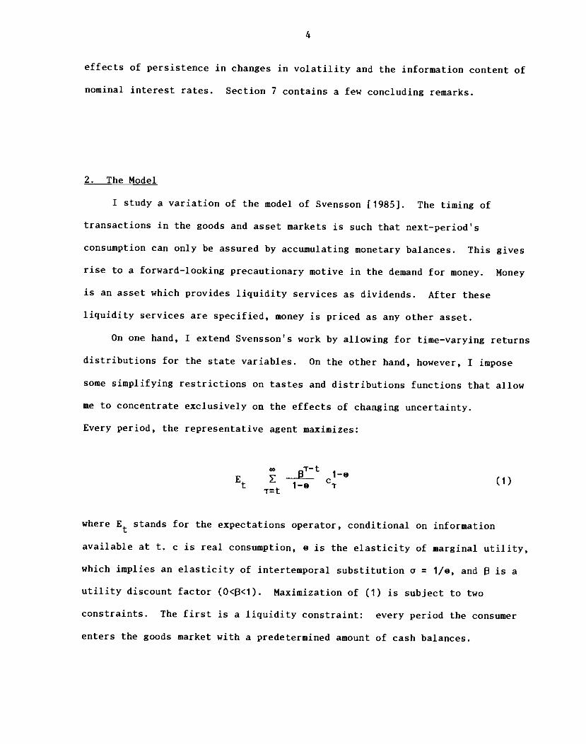
Every period, the representative agent maximizes:

E S cl_0 (1)t 1—0 '11t

where Et stands for the expectations operator, conditional on information

available at t. c is real consumption, a is the elasticity of marginal utility,

which implies an elasticity of intertemporal substitution a = 1/a, and is a

utility discount factor (O<U<1). Maximization of (1) is subject to two

constraints. The first is a liquidity constraint: every period the consumer

enters the goods market with a predetermined amount of cash balances.

5

Consumption can only be purchased with cash:

c (2)

where lit' the reciprocal of the nominal price level, is the purchasing power of

money (the price of 1 dollar in terms of the consumption good); Mt is the

predetermined amount of cash balances (which in equilibrium equals the

exogenously given nominal money stock, Mr).

After the goods market closes, the consumer enters the asset market. There

he receives a money transfer equal to where is the stochastic gross

rate of growth of the money stock, together with the gross return on his

holdings of the real asset, which equals (+Y)z. may be thought of as the

price of the stock of a single representative firm producing GNP with a

stochastic technology which uses no inputs. Thus is also the dividend on the

stock. z is the amount of the stock held by the consumer at the beginning of

the period. These resources, together with the leftover money balances from the

purchase of the consumption good, 1itMt_ct, are used to buy the real asset and

the nominal money balances to be carried through next period, Mt+i and

The budget constraint is thus:

litMt+i + + (+Y)z + (3)

which implicitly defines wealth as follows:

=TTtMt

+ (+Y)z +

Every period, the clearing conditions for the goods market, the asset

6

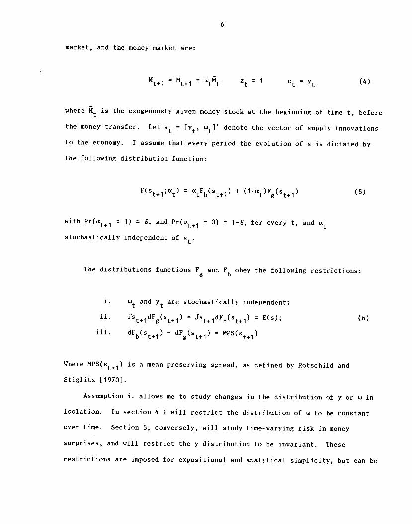
market, and the money market are:

= = = 1 c = (4)

where Mt is the exogenously given money stock at the beginning of time t, before

the money transfer. Let s = 3' denote the vector of supply innovations

to the economy. I assume that every period the evolution of s is dictated by

the following distribution function:

F(s+i;x) = aFb(s÷l) +t)Fg15t+i) (5)

with Proxt+i 1) = 8, and Pr(lx = 0) = 1—8, for every t, and

stochastically independent of s.

The distributions functions and Fb obey the following restrictions:

i and are stochastically independent;

= lst+ldFb(st+l) = E(s); (6)

iii. dFb(st+l) — dFg(St+i)=

MPS(s+1)

Where MPS(st+i) is a mean preserving spread, as defined by Rotschild and

Stiglitz [1970].

Assumption i. allows me to study changes in the distribution of y or w in

isolation. In section 4 I will restrict the distribution of w to be constant

over time. Section 5, conversely, will study time—varying risk in money

surprises, and will restrict the y distribution to be invariant. These

restrictions are imposed for expositional and analytical simplicity, but can be

7

released with little consequences. Assumption iii. is the central feature of

this paper. While the first moment of s is constant (from ii.), the probability

density function of s is more "spread out" when a equals 1, than when a equals

0: this is consistent with stochastically changing variances of dividends or

5money supply.

The i.i.d. "news" variable a is observed by the investor at the beginning

of each period, together with the current realization of s, and The

"news" variable tells him how much uncertainty there is in the economy.

Although the distribution of exogenous shocks is stochastically changing over

time, the investor——by observing a——knows for sure which distributions are next

period's innovations drawn from. Finally, notice that since a is i.i.d.

increases in uncertainty are purely temporary; and since F and Fb do not depend

on variables in s are i.i.d. both conditional on a and unconditionally.

As the analysis below makes clear, the fact that E(s) is constant does notimply that equilibrium expected returns are constant. Thus both first andsecond moments of returns are randomly fluctuating over time.

8

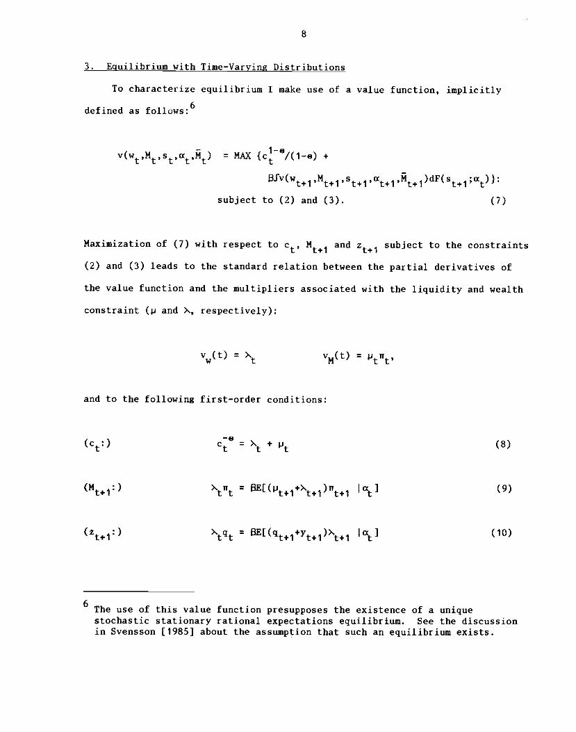
3. Equilibrium with Time—Varying Distributions

To characterize equilibrium I make use of a value function, implicitly

6defined as follows:

= MAX {c8/(l.e) +

subject to (2) and (3). (7)

Maximization of (7) with respect to c, Mt+i and z1 subject to the constraints

(2) and (3) leads to the standard relation between the partial derivatives of

the value function and the multipliers associated with the liquidity and wealth

constraint (p and >, respectively):

v(t) = vM(t) =

and to the following first—order conditions:

(cr:)—e

= >' + (8)

(M+i:) >' = HE[üit+i+Xt+i)lTt+i tI (9)

(zt+i:)= (10)

6The use of this value function presupposes the existence of a uniquestochastic stationary rational expectations equilibrium. See the discussionin Svensson [1985] about the assumption that such an equilibrium exists.

9

and:

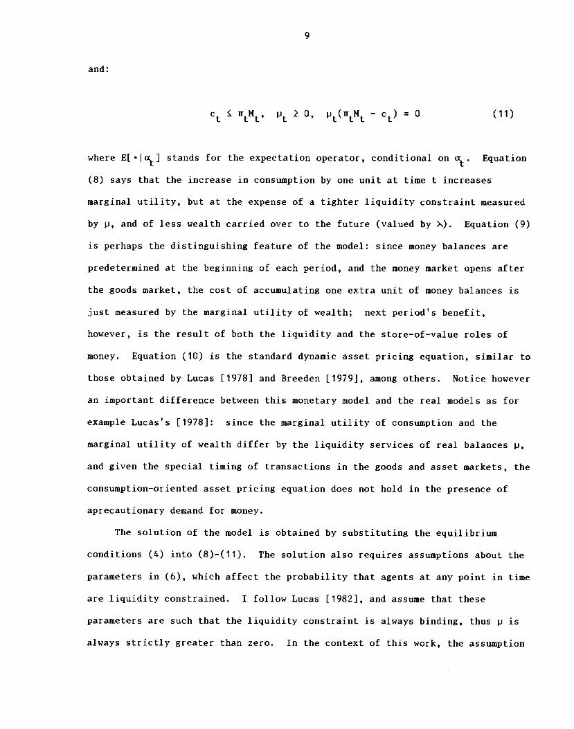
c utMt, ), — c) = 0 (11)

where E[.Ixt] stands for the expectation operator, conditional on x. Equation

(8) says that the increase in consumption by one unit at time t increases

marginal utility, but at the expense of a tighter liquidity constraint measured

by p. and of less wealth carried over to the future (valued by >). Equation (9)

is perhaps the distinguishing feature of the model: since money balances are

predetermined at the beginning of each period, and the money market opens after

the goods market, the cost of accumulating one extra unit of money balances is

just measured by the marginal utility of wealth; next period's benefit,

however, is the result of both the liquidity and the store—of—value roles of

money. Equation (10) is the standard dynamic asset pricing equation, similar to

those obtained by Lucas [19781 and Breeden [1979], among others. Notice however

an important difference between this monetary model and the real models as for

example Lucas's [1978]: since the marginal utility of consumption and the

marginal utility of wealth differ by the liquidity services of real balances p,

and given the special timing of transactions in the goods and asset markets, the

consumption-oriented asset pricing equation does not hold in the presence of

aprecautionary demand for money.

The solution of the model is obtained by substituting the equilibrium

conditions (4) into (8)—(11). The solution also requires assumptions about the

parameters in (6), which affect the probability that agents at any point in time

are liquidity constrained. I follow Lucas [1982], and assume that these

parameters are such that the liquidity constraint is always binding, thus p is

always strictly greater than zero. In the context of this work, the assumption

10

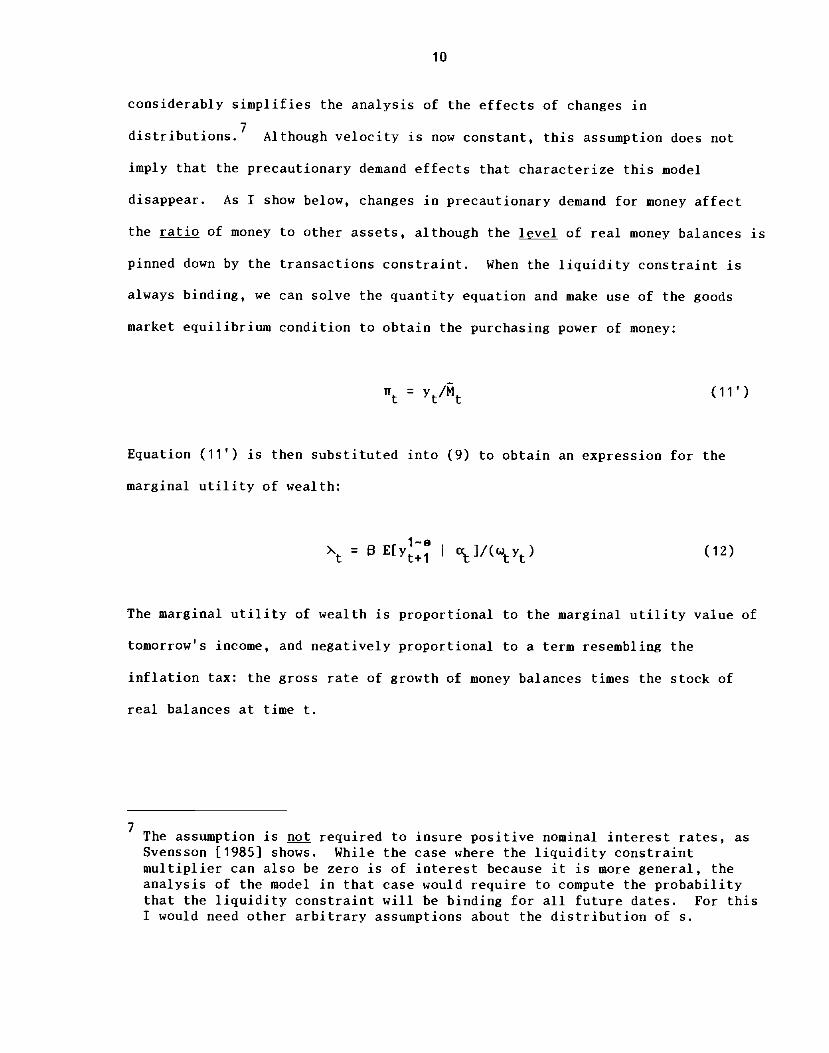
considerably simplifies the analysis of the effects of changes in

distributions.7 Although velocity is now constant, this assumption does not

imply that the precautionary demand effects that characterize this model

disappear. As I show below, changes in precautionary demand for money affect

the ratio of money to other assets, although the level of real money balances is

pinned down by the transactions constraint. When the liquidity constraint is

always binding, we can solve the quantity equation and make use of the goods

market equilibrium condition to obtain the purchasing power of money:

= (lit)

Equation (11') is then substituted into (9) to obtain an expression for the

marginal utility of wealth:

1—s= E[yt+i I (12)

The marginal utility of wealth is proportional to the marginal utility value of

tomorrow's income, and negatively proportional to a term resembling the

inflation tax: the gross rate of growth of money balances times the stock of

real balances at time t.

The assumption is not required to insure positive nominal interest rates, asSvensson [1985] shows. While the case where the liquidity constraintmultiplier can also be zero is of interest because it is more general, theanalysis of the model in that case would require to compute the probabilitythat the liquidity constraint will be binding for all future dates. For thisI would need other arbitrary assumptions about the distribution of s.

11

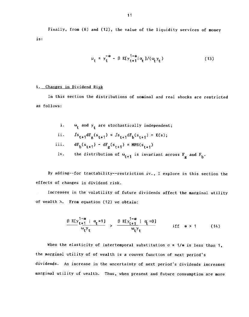
Finally, from (8) and (12), the value of the liquidity services of money

is:

—9 1-e—(13)

4. Changes in Dividend Risk

In this section the distributions of nominal and real shocks are restricted

as follows:

1. and y are stochastically independent;

ii. J'St+idFg(st+i) = fst+ldFb(st+l) = E(s);

iii. dFb(st+l) — dFg(St+i)=

MPS(s÷1)iv. the distribution of is invariant across F and F

t+1 g b

By adding——for tractability——restriction iv. , I explore in this section the

effects of changes in dividend risk.

Increases in the volatility of future dividends affect the marginal utility

of wealth X. From equation (12) we obtain:

1-e 1—9E[y1 a=l] E[yi> iff e 1 (14)

tt utyt

When the elasticity of intertemporal substitution a = lie is less than 1,

the marginal utility of of wealth is a convex function of next period's

dividends. An increase in the uncertainty of next period's dividends increases

marginal utility of wealth. Thus, when present and future consumption are more

12

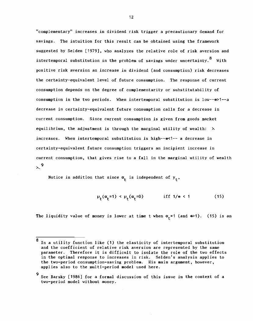
"complementary" increases in dividend risk trigger a precautionary demand for

savings. The intuition for this result can be obtained using the framework

suggested by Selden [1979], who analyzes the relative role of risk aversion and

intertemporal substitution in the problem of savings under uncertainty.8 With

positive risk aversion an increase in dividend (and consumption) risk decreases

the certainty-equivalent level of future consumption. The response of current

consumption depends on the degree of complementarity or substitutability of

consumption in the two periods. When intertemporal substitution is low——o>1——a

decrease in certainty—equivalent future consumption calls for a decrease in

current consumption. Since current consumption is given from goods market

equilibrium, the adjustment is through the marginal utility of wealth: >..

increases. When intertemporal substitution is high——e<1—— a decrease in

certainty—equivalent future consumption triggers an incipient increase in

current consumption, that gives rise to a fall in the marginal utility of wealth

Notice in addition that since oç is independent of y,

< p(oç=O) iff 1/s < 1 (15)

The liquidity value of money is lower at time t when x.=l (and s>1). (15) is an

8In a utility function like (1) the elasticity of intertemporal substitutionand the coefficient of relative risk aversion are represented by the sameparameter. Therefore it is difficult to isolate the role of the two effectsin the optimal response to increases in risk. Selden's analysis applies to

the two—period consumption—saving problem. His main argument, however,applies also to the multi—period model used here.

See Barsky [1986] for a formal discussion of this issue in the context of atwo—period model without money.

13

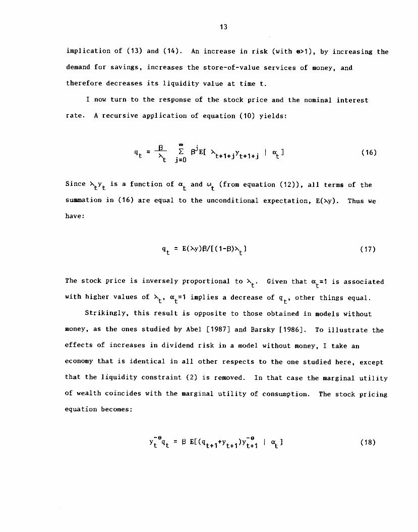
implication of (13) and (14). An increase in risk (with e>1), by increasing the

demand for savings, increases the store—of—value services of money, and

therefore decreases its liquidity value at time t.

I now turn to the response of the stock price and the nominal interest

rate. A recursive application of equation (10) yields:

--&E[ I o] (16)

Since is a function of and (from equation (12)), all terms of the

summation in (16) are equal to the unconditional expectation, E(Xy). Thus we

have:

= E(Xy)/[(1_)X] (17)

The stock price is inversely proportional to >• Given that is associated

with higher values of implies a decrease of other things equal.

Strikingly, this result is opposite to those obtained in models without

money, as the ones studied by Abel [1987] and Barsky [1986]. To illustrate the

effects of increases in dividend risk in a model without money, I take an

economy that is identical in all other respects to the one studied here, except

that the liquidity constraint (2) is removed. In that case the marginal utility

of wealth coincides with the marginal utility of consumption. The stock pricing

equation becomes:

=E{(÷1+Y1)Y91 (18)

14

and can be written as follows:

—8 -$ 1-9E[q1y1j ocI + E[y÷1 c] (19)

When 9>1 does increase the second term on the right—hand side of (19), but

leaves the first term unaffected, as a recursive application of (19) can

immediately show. Since the marginal utility of wealth is now given, the stock

price increases in response to higher dividend risk, when intertemporal

substitution is low (8>1). The reason why stock prices increase is the same as

the reason why the marginal utility of wealth increases in a monetary economy:

in both cases individual's desire to postpone consumption to next period has

gone up.

Why then do stock prices fall in the monetary economy? Unlike in the real

model of (18) and (19), shares are less liquid than money, and cannot be used to

provide for next period's consumption, since next period's asset market opens

after the goods market is closed. Indeed, the only way to shift consumption

from the current to the next period is to accumulate money balances.1° Thus if

intertemporal substitution is low the precautionary demand for money increases

when next period's dividend risk increases. An increase in dividend risk brings

about a portfolio shift out of stocks and into money. This effect is also

illustrated by the change in expected future liquidity services of money and the

nominal interest rate. A forward shift of equation (13) yields:

ljt+llrt+1 = = {y —E[Y+lXt+l]/Wt+l}/(Mt(.)t) (20)

10Of course the consumer can substitute present and future consumption beyondtime t+1 by accumulating any asset besides money.

15

Taking expectations of (20) conditional on information at time t, establishes

that the increase in expected liquidity services of money in response to higher

dividend risk is identically equal to the increase in the marginal utility of

wealth.

The increase in money demand generated by an increase in dividend risk-—

when intertemporal substitution is low——is also associated with higher nominal

interest rates. Following the procedure outlined by Lucas [1984] we can price

any asset in this economy, once its payoffs are clearly specified. In the case

of a one—period nominal bond, we need to determine——as Svensson [19851——the

nominal price of an asset which is purchased in the asset market at time t, at

the nominal price (1+it), and pays 1 unit of money when the asset market is

open at time t+1. Applying the pricing equations presented above yields:

=>stJT (21)

From equations (11') and (12) we have:

= E[Y+I%]/(Mta) (22)

Since \÷1+1 depends on E[X+1u+1cc] is independent of a. Thus from

(17) we have:

i (x=l) > i (cx=O)iff s > 1 (23)

The intuition for this result can be obtained by solving (21) after substituting

for with (9):

16

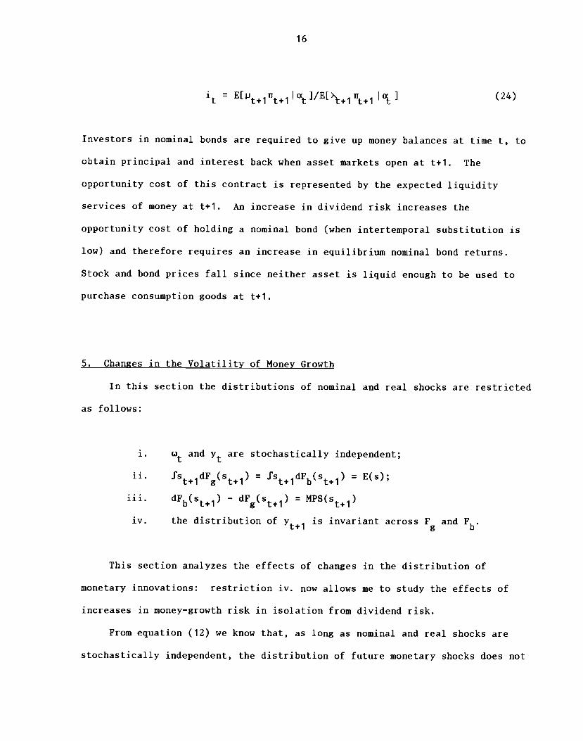
=E[lJt ilt ilt]/E[>s ill 1

(24)

Investors in nominal bonds are required to give up money balances at time t, to

obtain principal and interest back when asset markets open at t+l. The

opportunity cost of this contract is represented by the expected liquidity

services of money at t+1. An increase in dividend risk increases the

opportunity cost of holding a nominal bond (when intertemporal substitution is

low) and therefore requires an increase in equilibrium nominal bond returns.

Stock and bond prices fall since neither asset is liquid enough to be used to

purchase consumption goods at t+1.

5. Changes in the Volatility of Money Growth

In this section the distributions of nominal and real shocks are restricted

as follows:

and y are stochastically independent;

ii. •fSt+idFg(St+i) = Sst+ldFb(st+l) = E(s);

iii. dFb(st+l) — dFg(St+i)=

MPS(st+i)

iv. the distribution of is invariant across Fg and Fb.

This section analyzes the effects of changes in the distribution of

monetary innovations: restriction iv. now allows me to study the effects of

increases in money—growth risk in isolation from dividend risk.

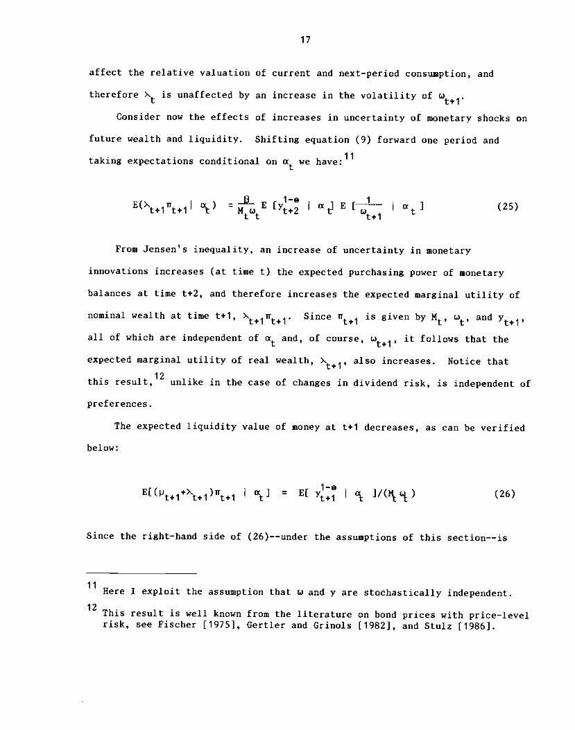
From equation (12) we know that, as long as nominal and real shocks are

stochastically independent, the distribution of future monetary shocks does not

17

affect the relative valuation of current and next—period consumption, and

therefore is unaffected by an increase in the volatility of

Consider now the effects of increases in uncertainty of monetary shocks on

future wealth and liquidity. Shifting equation (9) forward one period and

taking expectations conditional on we have:11

Di:) [y a E I 1 (25)

From Jensen's inequality, an increase of uncertainty in monetary

innovations increases (at time t) the expected purchasing power of monetary

balances at time t÷2, and therefore increases the expected marginal utility of

nominal wealth at time t+1, Since ir1 is given by Mt ' and

all of which are independent of x and, of course, w1, it follows that the

expected marginal utility of real wealth, also increases. Notice that

this result,12 unlike in the case of changes in dividend risk, is independent of

preferences.

The expected liquidity value of money at t+1 decreases, as can be verified

below:

I

ccc]= E[ I

cc ]/(frtctalt) (26)

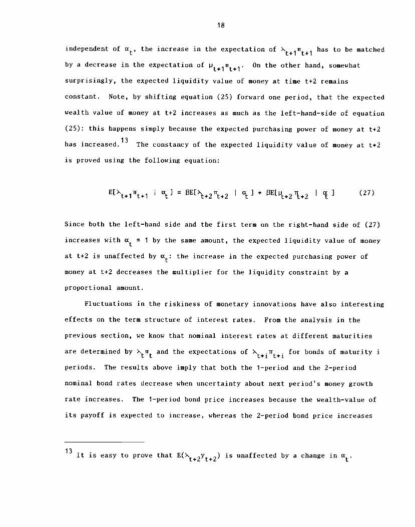
Since the right—hand side of (26)——under the assumptions of this section——is

Here I exploit the assumption that w and y are stochastically independent.

12This result is well known from the literature on bond prices with price—levelrisk, see Fischer [1975], Gertler and Grinols [1982], and Stulz [1986].

18

independent of a, the increase in the expectation of has to be matched

by a decrease in the expectation of On the other hand, somewhat

surprisingly, the expected liquidity value of money at time t÷2 remains

constant. Note, by shifting equation (25) forward one period, that the expected

wealth value of money at t+2 increases as much as the left—hand—side of equation

(25): this happens simply because the expected purchasing power of money at t÷2

has increased.13 The constancy of the expected liquidity value of money at t+2

is proved using the following equation:

E[Xt÷int+i= E[\+2ut+2 I cç] + E[vt+21x2 I ] (27)

Since both the left—hand side and the first term on the right—hand side of (27)

increases with = 1 by the same amount, the expected liquidity value of money

at t+2 is unaffected by a: the increase in the expected purchasing power of

money at t+2 decreases the multiplier for the liquidity constraint by a

proportional amount.

Fluctuations in the riskiness of monetary innovations have also interesting

effects on the term structure of interest rates. From the analysis in the

previous section, we know that nominal interest rates at different maturities

are determined by Xn and the expectations of for bonds of maturity i

periods. The results above imply that both the 1-period and the 2-period

nominal bond rates decrease when uncertainty about next period's money growth

rate increases. The 1—period bond price increases because the wealth—value of

its payoff is expected to increase, whereas the 2—period bond price increases

13It is easy to prove that E(X÷2y2) is unaffected by a change in

19

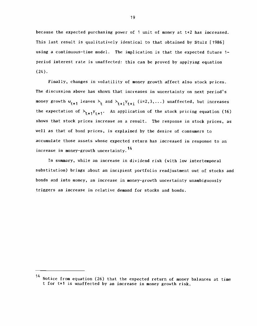
because the expected purchasing power of 1 unit of money at t+2 has increased.

This last result is qualitatively identical to that obtained by Stulz [19861

using a continuous—time model. The implication is that the expected future 1—

period interest rate is unaffected: this can be proved by applying equation

(24).

Finally, changes in volatility of money growth affect also stock prices.

The discussion above has shown that increases in uncertainty on next period's

money growth leaves and (i2,3,...) unaffected, but increases

the expectation of An application of the stock pricing equation (16)

shows that stock prices increase as a result. The response in stock prices, as

well as that of bond prices, is explained by the desire of consumers to

accumulate those assets whose expected return has increased in response to an

increase in money—growth uncertainty.14

In summary, while an increase in dividend risk (with low intertemporal

substitution) brings about an incipient portfolio readjustment out of stocks and

bonds and into money, an increase in money-growth uncertainty unambiguously

triggers an increase in relative demand for stocks and bonds.

14Notice from equation (26) that the expected return of money balances at timet for t+1 is unaffected by an increase in money growth risk.

20

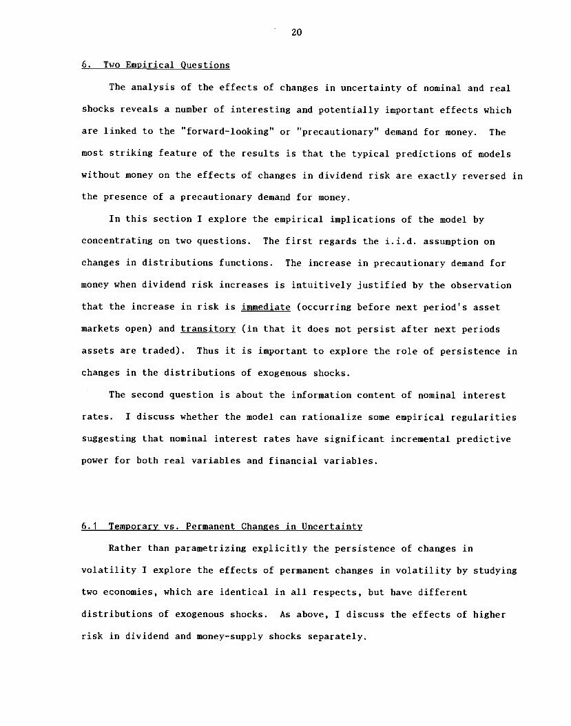
6. Two Empirical Questions

The analysis of the effects of changes in uncertainty of nominal and real

shocks reveals a number of interesting and potentially important effects which

are linked to the "forward-looking" or "precautionary" demand for money. The

most striking feature of the results is that the typical predictions of models

without money on the effects of changes in dividend risk are exactly reversed in

the presence of a precautionary demand for money.

In this section I explore the empirical implications of the model by

concentrating on two questions. The first regards the i.i.d. assumption on

changes in distributions functions. The increase in precautionary demand for

money when dividend risk increases is intuitively justified by the observation

that the increase in risk is immediate (occurring before next period's asset

markets open) and transitory (in that it does not persist after next periods

assets are traded). Thus it is important to explore the role of persistence in

changes in the distributions of exogenous shocks.

The second question is about the information content of nominal interest

rates. I discuss whether the model can rationalize some empirical regularities

suggesting that nominal interest rates have significant incremental predictive

power for both real variables and financial variables.

6.1 Temporary vs. Permanent Changes in Uncertainty

Rather than parametrizing explicitly the persistence of changes in

volatility I explore the effects of permanent changes in volatility by studying

two economies, which are identical in all respects, but have different

distributions of exogenous shocks. As above, I discuss the effects of higher

risk in dividend and money—supply shocks separately.

21

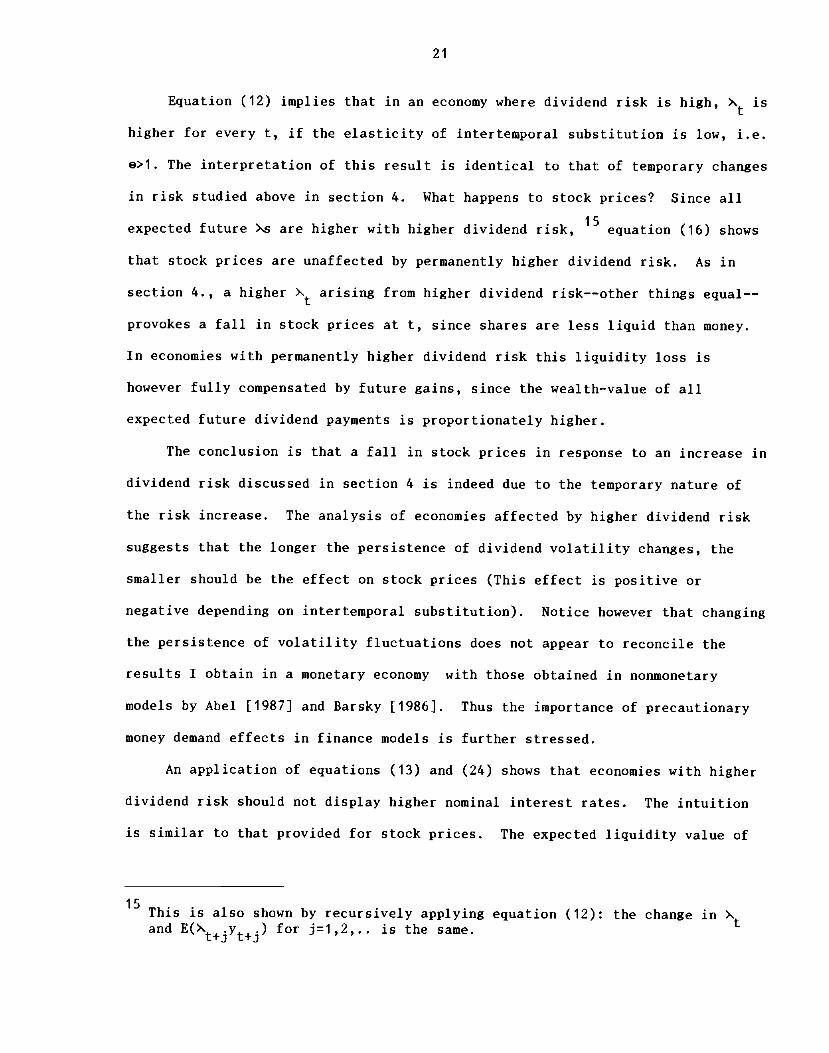
Equation (12) implies that in an economy where dividend risk is high, > is

higher for every t, if the elasticity of intertemporal substitution is low, i.e.

e>1. The interpretation of this result is identical to that of temporary changes

in risk studied above in section 4. What happens to stock prices? Since all

expected future >.s are higher with higher dividend risk,15

equation (16) shows

that stock prices are unaffected by permanently higher dividend risk. As in

section 4., a higher arising from higher dividend risk——other things equal——

provokes a fall in stock prices at t, since shares are less liquid than money.

In economies with permanently higher dividend risk this liquidity loss is

however fully compensated by future gains, since the wealth—value of all

expected future dividend payments is proportionately higher.

The conclusion is that a fall in stock prices in response to an increase in

dividend risk discussed in section 4 is indeed due to the temporary nature of

the risk increase. The analysis of economies affected by higher dividend risk

suggests that the longer the persistence of dividend volatility changes, the

smaller should be the effect on stock prices (This effect is positive or

negative depending on intertemporal substitution). Notice however that changing

the persistence of volatility fluctuations does not appear to reconcile the

results I obtain in a monetary economy with those obtained in nonmonetary

models by Abel [1987] and Barsky [1986]. Thus the importance of precautionary

money demand effects in finance models is further stressed.

An application of equations (13) and (24) shows that economies with higher

dividend risk should not display higher nominal interest rates. The intuition

is similar to that provided for stock prices. The expected liquidity value of

15This is also shown by recursively applying equation (12): the change in >and E(>..t+.yt+.) for j1,2,.. is the same.

22

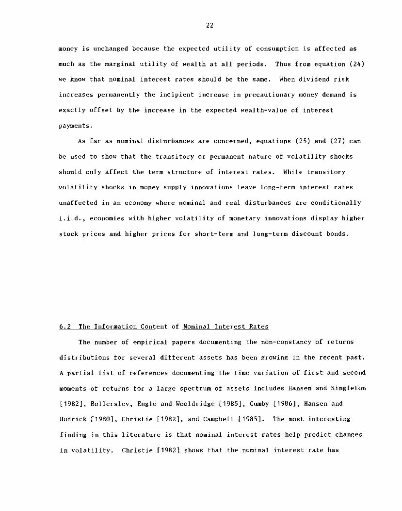
money is unchanged because the expected utility of consumption is affected as

much as the marginal utility of wealth at all periods. Thus from equation (24)

we know that nominal interest rates should be the same. When dividend risk

increases permanently the incipient increase in precautionary money demand is

exactly offset by the increase in the expected wealth—value of interest

payments.

As far as nominal disturbances are concerned, equations (25) and (27) can

be used to show that the transitory or permanent nature of volatility shocks

should only affect the term structure of interest rates. While transitory

volatility shocks in money supply innovations leave long—term interest rates

unaffected in an economy where nominal and real disturbances are conditionally

i.i.d., economies with higher volatility of monetary innovations display higher

stock prices and higher prices for short—term and long—term discount bonds.

6.2 The Information Content of Nominal Interest Rates

The number of empirical papers documenting the non—constancy of returns

distributions for several different assets has been growing in the recent past.

A partial list of references documenting the time variation of first and second

moments of returns for a large spectrum of assets includes Hansen and Singleton

[1982], Bollerslev, Engle and Wooldridge [1985], Cumby [1986], Hansen and

Hodrick [1980], Christie [19821, and Campbell [1985]. The most interesting

finding in this literature is that nominal interest rates help predict changes

in volatility. Christie [1982] shows that the nominal interest rate has

23

additional explanatory power over the debt/equity ratio in 354 out of 379

projection equations of the volatility of individual stock returns: an increase

in nominal interest rates is associated with a predictable increase in

volatility of stock returns. Giovannini and Jorion [1987] show that nominal

interest rates are positively correlated with the volatility of returns and

negatively correlated with nominal risk premia, both in the US stock market and

in the foreign exchange market. Additional evidence on the correlation of

nominal interest rates——or interest rate differentials——with volatility of

returns is provided by Cumby and Obstfeld [1984], and Hodrick and Srivastava

[1984]. Finally, Litterman and Weiss [1985] document an apparently puzzling

phenomenon, whereby nominal interest rates have incremental predictive power for

future macroeconomic variables, in such a way that cannot be easily justified

with the currently available families of macroeconomic models.

The model in this paper has important implications for the ability of

nominal interest rates to predict movements of conditional distributions of

exogenous shocks, and of the endogenous conditional second moments of asset

returns. Like Fama [1982] and Litterman and Weiss [1985], I consider a world

where the relevant information exceeds current and past observations of all real

and monetary variables: current information includes the knowledge of the degree

of uncertainty about future exogenous shocks. Changes in uncertainty, however,

are not directly observable.

The most important result is that, with i.i.d. shocks, nominal interest

rates are a sufficient statistic for the uncertainty in the economy, represented

by the uncertainty of nominal and real shocks. Indeed, nominal interest rates

are the best (and perfect) predictors of transitory changes in uncertainty. The

reason is that with constant i.i.d. distributions nominal interest rates are

constant in this model, as appears from equation (24). While this result would—

24

—of course——not hold in its current form if the i.i.d. assumption was relaxed,

its importance is that it suggests an economic interpretation of the evidence

from atheoretical projection equations. If intertemporal substitution is less

than 1, more uncertainty about future dividends induces agents to stay more

"liquid," by shifting out of stocks and bonds, and into money. As a result,

nominal interest rates increase, and stock prices fall. Thus the model can

reproduce and explain the findings by Christie [19821 and Giovannini and Jorion

[19871 that nominal interest rates are positively correlated with conditional

variances of returns.16

7. Concluding Remarks

This paper has studied some of the effects associated with the presence of

precautionary demand for money in a general—equilibrium asset pricing model.

Changes in dividend risk produce stock—price and interest-rate movements that

differ markedly from those that occur in the absence of precautionary money

demand. With low interemporal substitution, more dividend risk makes investors

want to stay more "liquid" and thus prompts a portfolio shift out of stocks and

into money. In the model, this effect makes interest rates predict next—period

dividend uncertainty more accurately than any other asset price. I also find

that changes in monetary-policy uncertainty affect both stock prices and nominal

interest rates.

The effects I illustrate in the paper appear worth exploring further, given

the nature of the empirical regularities that standard asset pricing models

16 A positive relationship between nominal interest rates and returns volatilityis additional evidence supporting the hypothesis that intertemporalsubstitution is empirically very low.

although their quantitative impact on short— and long—term interest rates might

be somewhat different.

25

empirical facts is of course

One shortcoming, however, is

cannot fully explain. The most important of these

the predictive content of nominal interest rates.

that some of the assumptions

empirically. Perhaps liquidi

assets rather than by money.

current monetary models, or t

shifts in agents' portfolios

discussed in finance models.

than cash, like Treasury bill

shifts I study in this paper

used in the model are arguably little plausible

ty services are performed in reality by short—term

My objective in this paper was not to criticize

o propose new ones: rather I wanted to identify

associated with phenomena that are not commonly

If liquidity services were offered by assets other

s or overnight deposits, the qualitative portfolio

would most likely still be present in some form,

26

References

Abel, A.B., "Stock Prices under Time-Varying Dividend Risk: An Exact Solutionin an Infinite—Horizon General Equilibrium Model," mimeo, The WhartonSchool of the University of Pennsylvania, February 1987.

Barsky, R.B., "Why Don't the Prices of Stocks and Bonds Move Together?"NBER Working ?aper No. 2047, October 1986.

Black, F., "Studies of Stock Price Volatility Changes," Proceedings of the 1976Meetings of the American Statistical Association, Business and EconomicStatistics Section, pp. 177—181.

Bollerslev, T.P., Engle, R. and Wooldridge, J.M., "A Capital Asset PricingModel with Time—Varying Covariances," mimeo, University of California atSan Diego, September 1985.

Breeden, D.T., "An Intertemporal Asset Pricing Model with StochasticConsumption and Investment Opportunities," Journal of FinancialEconomics, September 1979, 7: 265—296.

Campbell, John Y., "Stock Returns and the Term Structure," NBER Working Paperno. 1626, 1985.

Christie, A., "The Stochastic Behavior of Common Stock Variances," Journal ofFinancial Economics, December 1982, 10: 407—432.

Cumby, R.E., "Is It Risk? Explaining Deviations from Interest Rate Parity,"mimeo, New York University, October 1985.

Cumby, R.E. , and M. Obstfeld, "International Interest Rate and Price LevelLinkages Under Flexible Exchange Rates: A Review of Recent Evidence,"in J. Bilson and R. Marston, eds., Exchange Rate Theory and Practice,Chicago: University of Chicago Press, 1984.

Domowitz, I. and C.S. Hakkio, "Conditional Variance of the Risk Premium inthe Foreign Exchange Market," Journal of International Economics 19,August 1985, pp. 47—66.

Engle, R.F., D.M. Lilien, and R.P. Robins, "Estimating Time Varying RiskPremia in the Term Structure: The Arch—M Model," Econometrica, 55 no. 2,March 1987, pp. 391—408.

Fama, E.F., "Inflation, Output, and Money," Journal of Business, 1982, vol 55n. 2: 201—231.

Fischer, S. "The Demand for Indexed Bonds," ournal of Political Economy, 83,1975, pp. 509—534.

Gertler, M. and E. Grinols, "Monetary Randomness and Investment," Journal ofMonetary Economics 10, 1982, pp. 239—258.

27

Giovannini, A., "Time—Varying Distributions of Returns, Nominal Interest Ratesand Risk Premia in a Dynamic Asset Pricing Model," First Boston WorkingPaper n. 86—36, Columbia Business School, October 1986.

Giovannini, A. and P. Jorion, "Interest Rates and Risk Premia in the StockMarket and in the Foreign Exchange Market," Journal of InternationalMoney and Finance, March 1987, (forthcoming).

Hansen, L.P. and R.J. Hodrick, "Forward Exchange Rates as Optimal Predictorsof Future Spot Rates: An Econometric Analysis," Journal of PoliticalEconomy, October 1980, 88: 829—853.

Hansen, L.P. and K. Singleton, "Generalized Instrumental Variables Estimationof Nonlinear Rational Expectations Models," Econometrica, September 1982:50: 1269—86.

Hadrick, R.J. and S. Srivastava, "Risk and Return in Forward Foreign Exchange,"Journal of International Money and Finance, April 1984, 3: 5—29.

Litterman, R.B. and L. Weiss, "Money, Real Interest Rates, and Output: AReinterrpretation of Postwar U.S. Data," Econometrica, January 1985,vol. 53, n.1: 129—156.

Lucas, R.E., Jr., "Asset Prices in an Exchange Economy," Econometrica,November 1978, 46: 1429—1445.

, "Interest Rates and Currency Prices in a Two—CountryWorld," Journal of Monetary Economics, November 1982, 10: 335—360.

"Money in a Theory of Finance," Carnegie—Rochester ConferenceSeries on Public Policy, Volume 21, Autumn 1984: 9—46.

Malkiel, B., "The Capital Formation Problem in the United States," Journal ofFinance, 34, 1979, pp. 291—306.

Mascara, A. and A.H. Meltzer, "Long— and Short—Term Interest Rates in aRisky World," Journal of Monetary Economics, November 1983, 12: 485—518.

Pindyck, R.S., "Risk, Inflation, and the Stock Market," American EconomicReview, 74, June 1984, pp. 335—351.

Poterba, J.M. and L,H. Summers, "The Persistence of Volatility of StockMarket Fluctuations," American Economic Review, 76, December 1986,pp. 1142—1151.

Rothschild, M. and J.E. Stiglitz, "Increasing Risk: I. A Definition,"Journal of Economic Theory 1970 2: 225—243.

Selden, L., "An OCE Analysis of the Effect of Uncertainty on Saving underRisk Preference Independence," Review of Economic Studies, 46, 1979,pp. 73—82.

28

Stockman, A.C., "A Theory of Exchange Rate Determination," Journal ofPolitical Economy, August 1980, 88: 673—98.

Stulz, R.M., "Interest Rates and Monetary Policy Uncertainty," Journal ofMonetary Economics, May 1986, 17: 331—347.

Svensson, L.E.O., "Money and Asset Prices in a Cash-in-Advance Economy,"Journal of Political Economy, 93, no. 5, October 1985, Pp. 919—944.

Tobin, 3., "Liquidity Preference as Behavior Towards Risk," Review of EconomicStudies, 1958, pp. 65—86.

</ref_section>