Liquidity effects and market frictions

S. Hendry and G.J. Zhang

This paper was presented at the conference on General Equilibrium and Monetary Transmission, held at De Nederlandsche Bank, Amsterdam, 4-6 November 1998. The other papers presented at this conference are also published as DNB Staff Reports.

DNB Staff Reports 1999, No.29 De Nederlandsche Bank

©1999 De Nederlandsche Bank NV

Corresponding author: S. Hendrye-mail: shendry@bank-banque-canada.ca

Aim and scope of DNB Staff Reports are to disseminate research done by staff members of the Bank toencourage scholarly discussion.

Editorial Committee: Martin M.G. Fase (chairman), Peter van Bergeijk, Peter Koeze, Marga Peeters, Bram Scholten, Job Swank, Bert Groothoff (secretary).

Subscription orders for DNB Staff Reports and requests for specimen copies should be sent to:De Nederlandsche Bank NVExternal Relations and Information DepartmentWesteinde 1P.O. Box 981000 AB AmsterdamThe NetherlandsInternet: www.dnb.nl

Liquidity Effects and Markets Frictions

Scott Hendry and Guang-Jia Zhang

r-ist-

ricem-e

dif-ndthend-

lyry

ola-ntbeci--

ackversitye

e

,

LIQUIDITY EFFECTS AND MARKET FRICTIONS

Scott Hendry and Guang-Jia Zhang1

Abstract

The goal of this paper is to tackle two problems in standard limited-paticipation models: (1) an interest rate liquidity effect that is not as persent as in the data; and (2) nominal variables that are unrealisticallyvolatile. To address these problems, we introduce nominal wage and prigidities, as well as portfolio adjustment costs and monopolistically copetitive firms, to better understand how each of these costs affects thmodel economy.

Quantitative analysis shows that different adjustment costs have veryferent effects on the responses of the nominal interest rate, inflation aoutput. The model’s impulse response functions are more realistic in case with all three adjustment costs than any other case. The main fiings are: (1) limited-participation models generate too much liquidityeffect compared with the data; (2) portfolio adjustment costs are soleresponsible for the persistence of the liquidity effect following a monetapolicy action; (3) wage adjustment costs can help to reduce inflation vtility and increase output and inflation persistence; (4) price adjustmecosts are unable to significantly reduce inflation volatility; (5) there canimportant interactions between the adjustment costs; (6) limited-partipation models, even with additional adjustment costs, are still not successful in replicating the stylized facts for nominal variables.

We gratefully acknowledge the comments of Charles Carlstrom, Walter Engert, Michiel Keyzer, JSelody, and the seminar participants at De Nederlandsche Bank, the Bank of Canada, the Uniof Guelph, and the University of Quebec at Montreal. We thank Rebecca Szeto for her valuablresearch assistance.The views expressed in this paper are those of the authors. No responsibility for them should battributed to the Bank of Canada.

1 Corresponding authors: Scott Hendry and Guang-Jia ZhangDept. of Monetary and Financial Analysis, Bank of Canada, 234 Wellington St. Ottawa, OntarioCanada, K1A 0G9.e-mail: shendry@bank-banque-canada.ca gzhang@bank-banque-canada.ca

to itsis-

llyndardnsasthat

arys ofn

nts’tmentuldddi-itiesary

ky-nyllys aref these-our

theliocha-vel-

atejor

d tokers.

1 INTRODUCTION

Some economists argue that money plays a role in the economy dueasymmetric distribution to economic agents. That is, money is first dtributed to financial intermediaries and then to firms before it finareaches consumers’ hands. This is the basic idea embedded in a stalimited-participation model. However, there are still some limitatiowith the basic version of this model. First, the liquidity effect is notpersistent as that observed in the data. Most empirical estimates findthe interest rate should fall for a few quarters following an expansionmoney-growth shock. [See Figure 1.] Second, stochastic simulationlimited-participation models generally find too much volatility of inflatioand other nominal variables.

As we know, monetary policy shocks are transmitted through agedecision-making processes via dynamic mechanisms, such as adjuscosts. If markets operated without any frictions, monetary policies wohave no (persistent) effect on interest rates or any real variables. In ation, some economists have conjectured that price and wage rigidmay be a primary cause of the persistent liquidity effect of a monet

shock.2

In this vein, Christiano, Eichenbaum, and Evans (1996) compare sticprice models with limited-participation models. They conclude that amodel equipped with only one type of friction cannot successfuaccount for the basic stylized facts unless unrealistic parameter valueassumed. Aiyagari and Braun (1997) speculate that a combination olimited-participation model and a price- adjustment cost will lead to uful insights into business fluctuations. In this paper, we pursueresearch along this avenue. More precisely, we attempt to determinerelative importance of three major frictions -- price, wage and portfoadjustment costs -- in understanding the monetary transmission menism. Our model is based on the basic limited-participation model deoped by Christiano and Eichenbaum (1992b).

This paper introduces different types of adjustment costs to investigwhether they improve the model’s ability to replicate some of the ma

2 Aiyagari (1997) points out that a modelling approach that considers frictions can be expectehave a significant impact on answers to questions of interest to macroeconomists and policymaSee also Williamson (1996).

- 2 -

herthericee vol-

l, toosts

anda

costsine-heirngestsit

t to

ngesitsthetion

tingffec-nddel.

essetlyall

bothity

stylized facts of empirical impulse response functions and higmoments. First, portfolio-adjustment costs are introduced to prolonginterest-rate effects of a monetary policy shock. Second, nominal pand wage adjustment costs are also added to the model to dampen th

atility of the nominal side of the economy.3

In general, the adjustment costs we introduce do improve the modesome extent at least, in the expected manner. Portfolio adjustment care able to lengthen the interest rate liquidity effect while price costswage costs, in particular, are able to reduce inflation volatility followingmonetary policy action.

Wage adjustment costs, which can be thought of as wage negotiationor possibly information accumulation costs, are particularly effectivelowering the volatility of inflation by slowing wage increases and, consquently reducing any wage cost-push incentives for firms to increase tprices. With no price costs in the model, the wage cost does not chathe liquidity effect. However, if any price costs are present, wage cowill deepen the liquidity effect (i.e, lower the loan demand) by makingeasier for firms to avoid the price costs. This last result is in contrasresults generally found in other sticky wage models.

Portfolio adjustment costs reduce the incentives for households to chathe level of their cash holdings thereby limiting the adjustment of depoand creating a persistent liquidity effect. The extended deviation ofinterest rate from steady state induces a persistent deviation of inflaand output as well.

In contrast to the other costs, price adjustment costs (that is, markecosts, advertising costs, or information accumulation costs) are less etive, having only a minimal impact on inflation and output when wage aportfolio adjustment costs have already been introduced into the moIn particular, models with portfolio costs made price costs much leffective at reducing inflation volatility. In examples with only pricadjustment costs, there were reductions of inflation volatility, but mosin expected future volatility not the contemporary response. For sm

3 Dow (1995) has looked at the liquidity effects of monetary shocks by considering frictions in commodity and credit markets. Unfortunately, his model does not lead to more persistent liquideffects.

- 3 -

idityrsednces toty in

s aen-hema-ure

se-ds.stsardiosvex

price adjustment costs there is a deepening of the interest-rate liqueffect. However, as the costs are increased, the liquidity effect is reveas firms try to avoid the costs by increasing hours and output and heloan demand and the interest rate. In general, attempts by the firmavoid the price adjustment costs lead to excessive interest-rate volatilithe model.

The rest of this paper is organized as follows. Section 2 providedetailed description of the economic environment and the dynamic geral equilibrium problem of money. Section 3 calibrates the model. Tquantitative analysis is presented in Section 4. Finally, Section 5 sumrizes the findings in this paper, and points to the direction of our futresearch.

2 THE MODEL

2.1 Economic environment

2.1.1 Households

The preferences for a typical household,i (i=1,...,I), are given by:

(1)

where 0<β<1 and,

(2)

whereCit, Lsit, andACQ

it are the periodt consumption, labour supply, andtime cost of portfolio adjustment, respectively. We assume that houholds must take time to adjust their financial portfolios between perioThis assumption is different from the intra-period adjustment coassumption employed in Dotsey and Ireland (1995). As with the standlimited-participation models, households cannot adjust their portfolwithin a period. The portfolio adjustment cost is assumed to be a confunction of the following form:

E0 βtU Cit 1 Lit

s– ACit

Q–( , )

t 0=

∞

∑

U Cit 1 Lits

– ACitQ

–( , )1φ--- Cit 1 Lit

s– ACit

Q–( )

γ[ ]

φ=

- 4 -

stth

dy

-in-tionancecur-on-arde,

e

lize aandcan

as

(3)

whereϕq≥0 andQit is the amount of cash that householdi has at thebeginning of periodt. In deterministic steady state, the adjustment cowill be zero since all nominal variables will grow at the money grow

rate,1+x.4 As the growth rate of cash holdings deviates from its steastate level, the adjustment cost increases quadratically.

We assume that money is introduced into the economy by a cashadvance (CIA) constraint. That is, households make their consumpand investment purchases out of the sum of the nominal cash baltransferred from the last period and the labour income earned in therent period. This constraint is described in (4). The periodic budget cstraint is given by (5), which says that cash and deposits carried forwto periodt+1 is the sum of interest payments, dividends, capital incom

and unspent cash from the goods market.5

(4)

(5)

wherePt is the price level;Wt is the wage rate;Iit is periodt investment;Nit is the household’s level of demand deposits for periodt determined in

period t-1;6 Dit andFit are the dividends received from the firm and th

financial intermediaries, respectively, at the end of periodt; andACWit is

the wage adjustment cost. The rental price of capital is given byRkt sothat households earnRktKit from their capital stock in periodt.

We assume that a worker has to bear a real cost to propose and reachange in their nominal wages. We can think of this as a negotiatinginformation gathering costs. Even though the magnitude of the cost

4 This functional form is similar to that in Christiano and Eichenbaum (1992).5 Our model treats money primarily as a medium of exchange, even though other factors, suchvariation in velocity, might have important roles in the monetary transmission mechanism. Inaddition, a binding CIA constraint is not imposed in this model.6 The sum of cash and deposit holdings is equal to the money supply so that∑(Qit+Nit)=Mt.

ACitQ ϕq

2------

Qit 1+

Qit-------------- 1 x+( )–

2=

PtCit PtI it P+tACit

WQit Wit Lit+≤+

Qit 1+ Nit 1++ RtdNit Dit Fit RktKit

Qit Wit Lit PtCit– PtI it Pt ACitW

––+[ ]

+ + + +=

- 5 -

sig-al

ander a

neir

e

).

nal

theolyate,ndge

d

be small, the impact of the cost on aggregate labour supply might benificant. This wage adjustment cost is very different from the nominwage rigidities reflected in the long-term contracts between workersfirms. In this model, the wage can be changed at any time but only aftcost is paid.

During periodt, households take as given, from periodt-1, their capitalstock holdings (Kit) and their distribution of money holdings betweedeposits (Nit) and cash (Qit). Assume that households must choose thperiod t+1 split of financial assets between cash (Qit+1) and deposits(Nit+1) before the end of periodt. This is the standard assumption of thlimited-participation models.

The law of motion for the physical capital stock is given in equation (6

(6)

whereδ is the capital depreciation rate.

Wage adjustment costs are assumed to have the following functioform:

(7)

whereϕw≥0. The inclusion of the real wage ensures the real value ofcosts will grow with the economy. Since households have monoppower over their differentiated labour, they recognize that their wage rWit, is a function of their labour supply as shown below in (11) aaccount for this when maximizing their utility. Consequently, the waadjustment cost function can be written as a function ofLit by combining(7) and (11) below.

A household’s decision problem is to maximize utility given by (1) an

(2) by selecting decision variablesQit+1, Nit+1, Cit, Kit+1, andLsit subject

to the constraints in (3) to (7) and (11).

Kit 1+ 1 δ–( )Kit I it+=

ACitw Wt

Pt-------

ϕw2

-------Wit

Wit 1–------------------ 1 x+( )–

2

=

- 6 -

ichhemti-

usedodthe

.r-

uysr

2.1.2 The final goods firm

The final goods producer in this economy is simply an aggregator whbuys inputs from the intermediate goods producers and combines tinto the final good. Also, the aggregator hires labour from the differenated households to generate a composite labour commodity which isby intermediate goods firms in their production process. The final gocan either be consumed or invested. The production technology forfinal good is summarized by the followingconstant return to scalefunc-tion

(8)

whereYt is the output of the final good,Yjt is the amount of input acquiredfrom intermediate producerj, andJ is the number of intermediate firmsThe parameterθy is the elasticity of substitution between any two diffeent intermediate goods.

The final goods producer’s profit maximization problem is given as

(9)

From its first order condition forYjt, we can easily derive the followingsimple relation between the price,Pt, for the final good and the price,Pjt,charged by the producer of the intermediate goodj.

(10)

Following the same logic, we assume this final good producer also bheterogeneous labour,Lit, from householdi and sells a composite labou

input to the intermediate goods producers.7 Therefore, the relationshipbetween the competitive wage rate,Wt, faced by the firms and the individ-ual wage rate,Wit, set by householdi is given by

Yt J

11 θy–--------------

Yjt

θy 1–( )θy

-------------------

j 1=

J

∑

θy

θy 1–( )-------------------

=

Max Πt PtYt PjtY jtj 1=

J

∑–=

Pjt Pt

JYjt

Yt----------

1θy-----–

=

- 7 -

of

r

restheeatedurns

in

n beew

m

il-

y,

(11)

where θL is the elasticity of substitution between any two types

labour.8

2.1.3 The intermediate goods firms

Each intermediate good producerj (j=1,2,...,J) hires the aggregate labou

commodity available from the aggregator,Ldjt, in a perfectly competitive

market at wage rateWt. The firm also rents capital goods (Kjt) from thehouseholds, in a competitive market, at a rental price ofRkt. The firmmust borrow cash from the financial intermediary each period, at interateRt, in order to have the funds to hire labour and begin production. Tentire wage bill ofWtLjt must be borrowed before production occurs. Thcapital rental cost is assumed to be financed through internally generrevenue. Capital and labour inputs are combined in an increasing retto scale production function to produce a differentiated product,Yjt.

The firm sells its output in a monopolistically competitive marketwhich it has the power to set its own price,Pjt. However, we assume it iscostly for a firm to change the price of its product. These real costs cathought of as menu, advertising, or marketing costs for the setting of nprices.Firm j’s objective is to maximize the present value of its lifetime streaof dividend payments to its shareholders,Djt. These dividends are dis-counted by a factor,β, as well as by a term representing the marginal utity value of the dividends,λ2t, for the households, which own the firms.

7 The composite labour is produced by the aggregator with constant return to scale technolog

8 For simplicity, we will assume there is a unit mass of both households and firms.

Lt J

11 θl–-------------

l jt

θl 1–( )θl

------------------

j 1=

J

∑

θl

θl 1–( )------------------

=

Wit Wt

IL its

Lts

---------

1θL-----–

=

- 8 -

aytatetion

ur-

g

in

(12)

where

(13)

Let ACpjt represent a price adjustment cost which the firm must p

whenever it changes its price level at a rate different from the steady sgrowth rate. The price-adjustment cost function is described in equa(14).

(14)

whereϕp≥0. The presence of theYt term will ensure the costs will growwith rest of the economy.

The production technology exhibits increasing return to scale with laboaugmented technological progress, that is,

(15)

where 0<α<1 and Φ≥1. The variablezt represents labour-augmentintechnological progress following the process

(16)

The parameterη is the steady state growth rate of the technology levelthe economy and the technology shock,θt, is assumed to follow the ran-dom process,

(17)

This is a simple AR(1) process for which 0<ρθ<1 andεθt is i.i.d. withzero mean and standard deviationσθ.

max E0 βt λ2t D jt Ω1t⋅ ⋅t 0=

∞

∑

D jt Pjt Y jt Rt W⋅t

L jtd⋅ Rkt– K jt⋅– Pt ACjt

p⋅–⋅=

ACjtp

Yt

ϕp

2------

Pjt

Pjt 1–-------------- 1 x+

µ( )exp-----------------–

2

⋅=

Yjt F K jt L jtd,( ) K jt

αztL jt

d( )1 α–

( )Φ

= =

zt ηt θt+( )exp=

θt 1 ρθ–( )θ ρθθt 1– εθt+ +=

- 9 -

t of

dd.

rom

use-rom

ti-nd

bar-est

debt.

dis-

Firm j’s dividend-maximization problem can be characterized by a semarginal conditions for labour and capital as given in Appendix II.

2.1.4 Financial intermediary

At the beginning of periodt, the financial intermediary has demandeposits ofNt that it received from the households in the previous perioThe financial intermediary uses these funds, along with any transfer f

the government,Xt, to make loans to the intermediate firms,Bft.

(18)

At the end of each period, the financial intermediary pays back the hohold deposits, with interest, using the debt repayments collected f

firms.9 The objective of the financial intermediary is to choose the opmal amount of loans made to firms and the optimal level of demadeposits to maximize the expected present value of its dividend:

(19)

where the dividend is given by,

(20)

Financial intermediation is assumed to be a costless activity. With noriers to entry, competitive forces will ensure that the equilibrium inter

rate on loans equals the rate paid on deposits, that isRlt=Rd

t=Rt. Conse-quently, in equilibrium, the financial intermediary will payFt=(1+Rt)Xt

in dividends to the households.

2.1.5 The central bank and government

We assume that the government neither collects taxes nor issuesHowever, the government makes transfer,Xt=Mt+1-Mt, to the financialintermediaries through the central bank. In this case, new money is

9 We assume that there is no risk of default in this model.

Btf

Nt Xt+=

max E0 βtλ2tFtt 0=

∞

∑

Ft 1 Rtl

+( )Btf

1 Rtd

+( )Nt–=

- 10 -

he

as

-ialof

nks

onslib-

h

tributed directly by the central bank to only financial institutions.10 Thisrestriction on how money is distributed provides the motivation for tnon-neutrality of money in the short run in this model.

Assume that the central bank follows a money growth rate ruledescribed in equation (21)

(21)

wherext is the money growth rate,Xt/Mt.

An exogenous positive monetary shock,εxt>0, increases the funds available to the financial intermediary in period t. Consequently, the financintermediary responds by lending more to firms for the employmentlabour. To ensure that firms will borrow these excess fund, the balower the equilibrium interest rate thereby creating the liquidity effect.

2.1.6 Market clearing

Assuming a unit mass of households and firms, the following equatidescribe the market-clearing conditions which must hold for an equirium to exist:(1) Goods:

(22)

(2) Loans:

(23)

(3) Money:

(24)

(4) Labour:

(25)

10 In Canada, monetary expansions and contractions are carried out by the central bank’s casmanagement: drawdowns and redeposits of federal government deposits with direct clearers.

xt 1 ρx–( )x ρxxt 1– εxt+ +=

Ct I t ACtw

ACtp

+ + + Yt=

WtLt Nt Xt+=

Mt 1+ Mt Xt+=

Lts

Ltd

=

- 11 -

llo-

diancap-

eizedal-

a

RS)s-to-996)

2.2 Equilibrium

A stationary competitive equilibrium is defined to be a sequence of a

cations Cit, Lsit, Nit+1, Qit+1, Iit for households, Kjt, Ld

it for firms, aset of prices Pit, Pt; Wjt, Wt; Rt; Rkt, and a central bank reaction function xt such that, given the equilibrium prices and other parties’ actions,

(1) households choose Cit, Lsit, Nit+1, Qit+1, Iit, Wit to maximize (1)

subject to constraints (2) to (7) and (11);

(2) firms choose Kjt, Ldit, Pjt to maximize (12) subject to constraints

(13) to (17);

(3) financial intermediaries solve the maximization problem in (19);

(4) prices adjust to ensure that market-clearing conditions hold:Pt clearsthe final-goods market,Wt clears the composite labour market,Rt clearsthe loan (or credit) market.

3 CALIBRATION

The balanced growth path of the model is calibrated to quarterly Canadata for the 1955 to 1996 period. The mean annual growth rate of perita output during this period was 1.83%, so we setµ=0.004563 (1.83% =(exp(µ)-1)*4). The discount factorβ was assumed to be 0.993, so thannual real rate of return on investment is about 2.8%. The annualdepreciation rate,δ, was set at 10% to approximately match the capitoutput ratio observed in the Canadian data.

The parametersθy and θl represent the market power that a firm andhousehold have to adjust their price and wage, respectively. Smallerθ val-ues represent stronger market power. A constant-return-to-scale (Ceconomy would set theseθ values to infinity so that firms and householdwould be price and wage takers. However, with an increasing-returnscale (IRS) economy we choose values closer to those used in Kim (1

- 12 -

ateas-

a.

qual

llow

tent.dard6).

roc-wth

Thisrythe

tate,

ut 16.38ings

thearly,a-ut.

ulse

ave

and setθy=5.0 andθl=10.0.11 The increasing return to scale parameter,Φ,is set at a moderate value of only 1.25. Finn (1995) has suggested thΦshould not be too large because the volatility of real variables is decring in the degree of IRS. The value ofα=0.3369 is chosen such that thesteady state labour share of income is 0.65, which is found in the dat

The preference parametersγ=3.8068 andφ=−0.4213 are calibrated suchthat the steady state employment and consumption-output ratio are e

to 0.171 and 0.745, respectively, as observed in the Canadian data.12

As described in equation (17), the technology shock is assumed to foan AR(1) process. The autocorrelation parameter,ρθ, is set to be 0.95based on the assumption that the technology shock is fairly persisThe standard deviation of the technology shock is set so that the standeviation of output from the model is close to that from the data (0.016

The monetary policy parameters describing the money growth rate pess from equation (21) are calibrated to match the quarterly mean grorate and autocorrelation coefficient of the Canadian money base.implies x=0.011 andρx=0.18. The standard deviation of the monetapolicy shock is set such that the variance of money growth rate frommodel is close to that from the data (0.0096).

For the adjustment-cost parameters, which do not affect the steady swe assumeϕp=1, ϕw=10, andϕq=1. If the model’s time endowment ofone unit per period represents 1460 hours per quarter in real time abohours per day, thenϕq=1 indicates that a household spends an extra 4minutes on portfolio adjustment when the desired change in cash holddeviates by 1% from the steady state change. A value ofϕw=10 impliesthat a worker pays 0.05% of his/her quarterly real wage rate to changenominal wage rate by 1% different than the steady state change. Similif a firm wants to adjust its price level by 1% more than the steady infltion rate, it has to pay a cost equivalent to 0.005% of its quarterly outpThese values were chosen to yield reasonably persistent impresponses for a monetary policy action.

11 Our model structure is fairly similar to that in Kim (1996).12 The consumption-output ratio may seem high since government and private consumption hbeen lumped together for simplicity.

- 13 -

55Q1ailedardllsthisnd, thentifi-ree

forcyfla-foreck.anse

does

el’sova-

theto 7thests,e 5

illus-tionhen

4 RESULTS

4.1 Some stylized facts on liquidity effects in Canada

We present a vector autoregressive analysis of the Canadian data (19to 1996Q4) in Figure 1. These basic results summarize the more detanalysis from Fung and Kasumovich (1998). Following a one standdeviation shock to M1 growth, the short-term nominal interest rate faimmediately by about 30 basis points. In the subsequent quarters,liquidity effect becomes dominated by the expected inflation effect athe interest rate starts to increase gradually. After about eight quartersinterest rate moves above steady state. The various policy shock idecation techniques usually estimate liquidity effects that last between thand six quarters for Canada.

The low interest rate leads to an extended expansion of output lastingthree to four years (following an initial perverse decline). The polishock has an immediate impact on inflation in the first quarter. The intion responds immediately then falls back toward steady state bejumping up again to another peak about six quarters following the shoThe deviation of inflation from steady state persists for much longer thoutput. Other VAR identification techniques can find no initial responof inflation followed by an extended increase above steady state thatnot start until as many as four quarters after the shock.

4.2 Expansionary policy action: impulse response functions

This section analyses the model through a discussion of the modimpulse responses to a one period monetary policy action. The inntion, εxt, in equation (21) is set to 0.01, representing a 4 per cent annual-ized money growth rate shock. The impulse response functions forinterest rate, inflation rate, and output are plotted in each of Figures 2for different adjustment cost assumptions. Figures 2, 3, and 4 showimpulse responses when portfolio, wage, and price adjustment corespectively, are added to the basic limited-participation model. Figurshows the model responses when all of the costs are combined. Totrate that the model can respond differently depending on the combinaof costs assumed, Figure 6 shows the effects of adding wage costs w

- 14 -

to a

ion

edall

l ofmesendtorthewer

madeeenin

ostsameriodperi-

tageasiserall

uchpply

in

folios

there are also price costs present while Figure 7 adds price costsmodel with portfolio costs.

Portfolio adjustment costs:

The base case in Figure 2 is a model with just the limited-participat

assumption.13 This model generates too much liquidity effect comparwith the Canadian data. In addition, the effects of a policy action onvariables are short lived.

However, once the inter-period portfolio adjustment cost is added althe responses become much more persistent. The liquidity effect becovery persistent because financial institutions stay flush with cash to lfor a much longer period. By holding the funds in the banking seclonger, the portfolio costs delay the demand side price pressure fromexpansionary shock. Consequently, the inflation response is much loand more persistent. The output response is also dampened andmuch more persistent. The effects of this type of portfolio cost have billustrated by other authors as well. The contribution of this paper liesthe addition of other nominal rigidities to the model.

Wage adjustment costs:

Figure 3 illustrates the effects of introducing the wage adjustment cinto the model when no other costs are present. The base case is theas in Figure 2. The wage adjustment cost has no effect on the first peresponse of the interest rate but it does raise the rate in subsequentods. The initial response of inflation is reduced by about one percenpoint while the second period response is reduced by about 50 bpoints. Subsequently, the inflation response is larger so that the oveffect of the wage cost is to delay the inflation response.

The output response is strengthened substantially and becomes mmore persistent. The wage cost makes households more willing to sulabour. Therefore, for a given shock, there will be a larger increaselabour and output and less of an increase in wages and prices.

13 All of the models discussed maintain the assumption that households cannot adjust their portwithin a period. The case without portfolio costs assumes no inter-period adjustment cost (ϕq=0) butstill maintains the infinite intra-period cost.

- 15 -

mentlit-

ndbse-rgerakes

ine-and

thepen-esd theysisforer as

thes atinfla-bse-uch

just-odelsults

ini-t.pen-s

ela-restthe

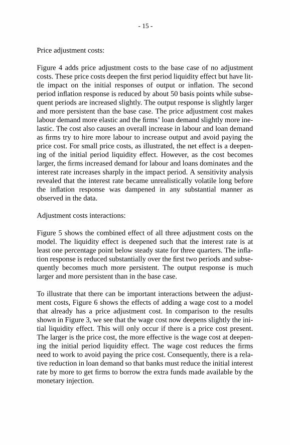
Price adjustment costs:

Figure 4 adds price adjustment costs to the base case of no adjustcosts. These price costs deepen the first period liquidity effect but havetle impact on the initial responses of output or inflation. The secoperiod inflation response is reduced by about 50 basis points while suquent periods are increased slightly. The output response is slightly laand more persistent than the base case. The price adjustment cost mlabour demand more elastic and the firms’ loan demand slightly morelastic. The cost also causes an overall increase in labour and loan demas firms try to hire more labour to increase output and avoid payingprice cost. For small price costs, as illustrated, the net effect is a deeing of the initial period liquidity effect. However, as the cost becomlarger, the firms increased demand for labour and loans dominates aninterest rate increases sharply in the impact period. A sensitivity analrevealed that the interest rate became unrealistically volatile long bethe inflation response was dampened in any substantial manneobserved in the data.

Adjustment costs interactions:

Figure 5 shows the combined effect of all three adjustment costs onmodel. The liquidity effect is deepened such that the interest rate ileast one percentage point below steady state for three quarters. Thetion response is reduced substantially over the first two periods and suquently becomes much more persistent. The output response is mlarger and more persistent than in the base case.

To illustrate that there can be important interactions between the adment costs, Figure 6 shows the effects of adding a wage cost to a mthat already has a price adjustment cost. In comparison to the reshown in Figure 3, we see that the wage cost now deepens slightly thetial liquidity effect. This will only occur if there is a price cost presenThe larger is the price cost, the more effective is the wage cost at deeing the initial period liquidity effect. The wage cost reduces the firmneed to work to avoid paying the price cost. Consequently, there is a rtive reduction in loan demand so that banks must reduce the initial interate by more to get firms to borrow the extra funds made available bymonetary injection.

- 16 -

ort-y nog-e

idityice

s infor

ostsvar-inalheandice

ver-ch

996edput;

atartainbleostsbyst-

evia-na-

le as

Figure 7 shows the effects of adding a price adjustment cost when a pfolio cost is also present. Here, we see that the price cost has virtuallability to reduce inflation volatility in contrast to the results shown in Fiure 4. Also, the liquidity effect is now reduced in the first period while thprevious analysis showed that the price cost could deepen the liqueffect. In general, greater portfolio costs reduced the ability of the prcosts to lower inflation volatility.

Overall, the adjustment costs improve the model’s impulse responsethe intended manner. However, the results were much more promisingthe portfolio and wage costs than for the price costs. The former two creduce nominal volatility and make the responses of real and nominaliables much more persistent while the price costs have only a margeffect on inflation and a much larger impact on the interest rate. Tmodel also reveals some important interactions between the wageprice costs. Wage costs can deepen the liquidity effect but only if prcosts are present.

4.3 Higher moments

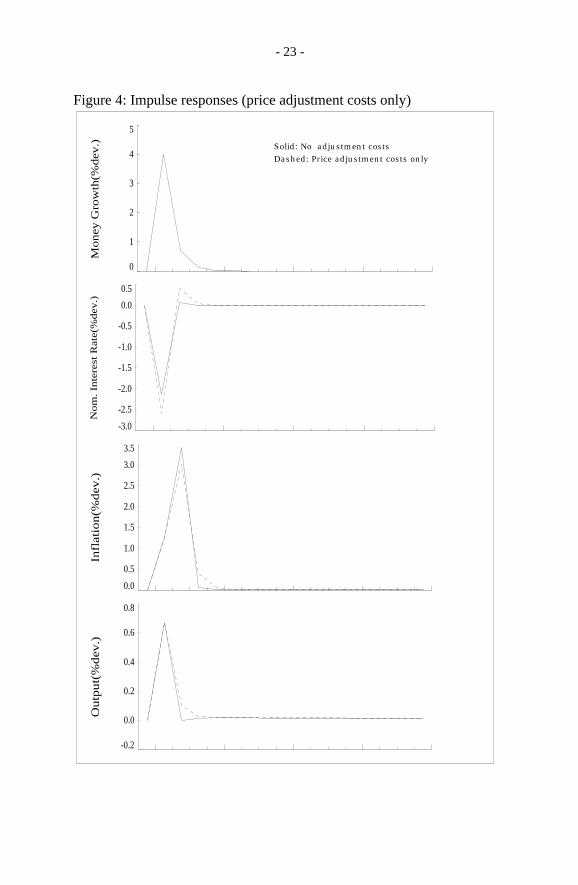
This section analyses the higher moments of a number of differentsions of the model to illustrate some of the relative contributions of eaof the adjustment costs.Table 1 contains some summary statistics for Canada from 1955 to 1for the primary real and nominal variables. Some of the main stylizfacts are: (1) interest rate is quite smooth; (2) price is as volatile as out(3) inflation is more variable than output.

A 42-year sample was replicated 50 times assumingσθ=0.01 andσx=0.0096. The model’s trend was reintroduced into the simulated dbefore it was logged and HP detrended. The summary statistics for cevariables of interest are given in Table 2. The first set of columns in Ta2 shows the results of the model when there are no adjustment cincluded. The next two columns add price adjustment costs, followedwage adjustment costs, and finally, in the last column, portfolio adjument costs are added.

On the real side, comparing Tables 1 and 2 shows that the standard dtions of output and consumption are quite close to that found in the Cadian data although the simulated investment series are not as volati

- 17 -

eralof

redop-ersofna-themestil-

ddi-le 2.ort-entto

tion

te,ga-er-thesionee into

with

rre-oliorateThe

tfo-eallythatutput

the and a

they should be. In general, our model, like the other dynamic genequilibrium models, can mimic reasonably well the cyclical behaviorthe real economy.

On the nominal side, all nominal variables are more volatile compawith their counterparts in the data. This is caused partially by the monolistic-competition structure, where workers and intermediate producare not price takers. All three adjustment costs reduce the volatilityinflation but not by enough to replicate the variance observed in the Cadian data. The price adjustment costs greatly increase the volatility ofnominal interest rate. This implies that the real interest rate also becomore volatile given that price adjustment costs reduce the inflation volaity. This is one reason the real variables also fluctuate more with the ation of price adjustment costs, as shown in the second column of TabThe last two columns of the table present the effect of the wage and pfolio adjustment costs. It is clear that the wage and portfolio adjustmcosts offset some of the volatility of the interest rate, but not enoughallow the price adjustment costs to be increased until the model’s inflavolatility matched the Canadian data.

All versions of the model exhibit negative correlations of the interest raprice level, and inflation rate with output while the actual data has a netive correlation between only output and the price level. This is detmined by the basic feature of a limited-participation model, that is,strong negative correlation between interest rate and output. The incluof the adjustment costs strengthens this negative relation, as we can sTable 2. As well, the wage adjustment costs are most useful for tryingreverse the negative correlations of the inflation rate and interest rate

output.14 The basic version of the model also has a negatively autocolated interest rate, contrary to the Canadian data, which the portfadjustment cost is capable of reversing. However, the actual interestwas still much more persistent than could be generated by the model.inflation rate in the model was also negatively autocorrelated until porlio adjustment costs were added, but, again, none of the costs could rcreate the desired degree of inflation persistence. Our findings implythe market adjustment costs can help generate the persistence in o

14 In a version of the model in which firms owned capital instead of households, the inclusion ofwage adjustment cost generates results with a positive correlation between inflation and outputnegative correlation between the price level and output, as in the data.

- 18 -

inal

thealulsetici-

ityst,the

d-onpricethe

bourrices.n

just-cing

el.ge

y if

ouseyet-

hertrally

fluctuation, but cannot successfully replicate the variation of the nomside of the Canadian economy.

5 CONCLUDING REMARKS

This paper examines how different types of market frictions can affecttransmission of monetary policy. It is shown that different types of reand nominal side adjustment costs can be used to improve the impresponse functions and higher moment characteristics of limited-parpation models.

The price adjustment cost could not effectively reduce inflation volatilwithout first introducing excessive interest rate volatility. In contrawage and portfolio adjustment costs are relatively more effective thanprice rigidity at reducing the nominal volatility in the economy. For moest levels of price adjustment costs, this relative inability to lower inflatioccurs because the changes in the firm’s behaviour caused by thecost create subsequent effects that offset the firm’s desire to minimizeprice cost. For instance, higher price adjustment costs increase lademand which pushes up wages and hence consumer demand and pThese offsetting effects limit the price cost’s ability to reduce inflatiovolatility in this model.

The model also reveals some important interactions between the adment costs. Price adjustment costs were even less effective at reduinflation volatility when there were portfolio costs present in the modAlso, in contrast to results found in the sticky wage literature, the waadjustment costs could deepen the liquidity effect in this model but onlthere were price adjustment costs already present.

Future research will extend the current model by considering varispecifications of the monetary policy reaction function, including mongrowth rules, interest rate rules, as well as inflation or price level targing. In particular, the policy rules would be ranked to determine whetan inflation-targeting rule dominates the others according to a cenbanks objective function. Also it would be interesting to complete

- 19 -

mal

cu-of

the

endogenize the money growth rule and determine the globally optipolicy reaction function when faced with a particular set of shocks.

Another related extension would be to incorporate a more finely artilated banking sector, which would inform our understanding of the rolefinancial intermediation, and the interaction of money and credit, intransmission of monetary policy.

- 20 -

996)

Figure 1: Impulse response functions for the Canadian data (1955 - 1In

tere

st R

ate

(%)

Infla

tion

(%)

M1

Gro

wth

(%)

GD

P (%

)

- 21 -

Figure 2: Impulse responses (portfolio adjustment costs only)

0

1

2

3

4

5

Mo

ne

y G

row

th(%

de

v.)

-2.5

-2.0

-1.5

-1.0

-0.5

0.0

0.5

No

m.

Inte

rest

Ra

te(%

de

v.)

0.0

0.5

1.0

1.5

2.0

2.5

3.0

3.5

Infla

tio

n(%

de

v.)

-0.2

0.0

0.2

0.4

0.6

0.8

Ou

tpu

t(%

de

v.)

Solid: No adjustment costs

Dashed: Portfolio adjustment costs only

- 22 -

Figure 3: Impulse responses (wage adjustment costs only)

0

1

2

3

4

5

Mo

ne

y G

row

th(%

de

v.)

-2.5

-2.0

-1.5

-1.0

-0.5

0.0

0.5

1.0

No

m.

Inte

rest

Ra

te(%

de

v.)

-1

0

1

2

3

4

Infla

tio

n(%

de

v.)

-0.2

0.0

0.2

0.4

0.6

0.8

1.0

1.2

Ou

tpu

t(%

de

v.)

Solid: No adjustment costs

Dashed: Wage adjustment costs only

- 23 -

Figure 4: Impulse responses (price adjustment costs only)

0

1

2

3

4

5

Mo

ne

y G

row

th(%

de

v.)

-3.0

-2.5

-2.0

-1.5

-1.0

-0.5

0.0

0.5

No

m.

Inte

rest

Ra

te(%

de

v.)

0.0

0.5

1.0

1.5

2.0

2.5

3.0

3.5

Infla

tio

n(%

de

v.)

-0.2

0.0

0.2

0.4

0.6

0.8

Ou

tpu

t(%

de

v.)

Dashed: Price adjustment costs onlySolid: No adjustment costs

- 24 -

Figure 5: Impulse responses (all adjustment costs)

0

1

2

3

4

5

Mo

ne

y G

row

th(%

de

v.)

-3.0

-2.5

-2.0

-1.5

-1.0

-0.5

0.0

0.5

No

m.

Inte

rest

Ra

te(%

de

v.)

-1

0

1

2

3

4

Infla

tio

n(%

de

v.)

-0.2

0.0

0.2

0.4

0.6

0.8

1.0

1.2

Ou

tpu

t(%

de

v.)

Solid: No adjustment costsDashed: All adjustment costs

- 25 -

Figure 6: Impulse responses (wage and price adjustment costs)

0

1

2

3

4

5

Mo

ne

y G

row

th(%

de

v.)

-3

-2

-1

0

1

No

m.

Inte

rest

Ra

te(%

de

v.)

-1

0

1

2

3

4

Infla

tio

n(%

de

v.)

0.0

0.2

0.4

0.6

0.8

1.0

1.2

Ou

tpu

t(%

de

v.)

Dashed: Wage and price adjustment costs

Solid: Price adjustment costs only

- 26 -

Figure 7: Impulse responses (price and portfolio adjustment costs)

0

1

2

3

4

5

Mo

ne

y G

row

th(%

de

v.)

-2.5

-2.0

-1.5

-1.0

-0.5

0.0

0.5

No

m.

Inte

rest

Ra

te(%

de

v.)

0.0

0.5

1.0

1.5

2.0

Infla

tio

n(%

de

v.)

0.0

0.1

0.2

0.3

0.4

0.5

0.6

Ou

tpu

t(%

de

v.)

Solid: Portfolio adjustment costsDashed: Price and portfolio adj. costs

- 27 -

relation

erest rate and thespans the 1976 to

2

.60

.77

93

0.18

.75

94

2

Table 1 Cyclical behaviour of the Canadian economy: 1955:01 to 1996:04

Variables

StandardDeviation

(%)Correlation with

real GDP Autocor

Real:a

a. All the real variables and the price level are logged and then HP detrended. Money growth, the intinflation rate are HP detrended. The real variables are in per capita terms. The data on hours worked1996 period only. We also apply this same procedure to the time series generated from the model.

GDP 1.66 1.00 0.8

Consumption 0.75 0.61 0

Investment 5.38 0.88 0

Hours 1.85 0.85 0.

Nominal:

Money base growth rate 0.96 0.07

Interest rate 0.38 0.32 0

Price 1.40 -0.45 0.

Inflation 1.93 0.29 0.4

- 28 -

Table 2 Cyclical b

Variables

Add portfolio adj. costs(ϕp=1; ϕw=10;ϕq=1)

S.(%

S.D.(%)

Corr.withY

Autocorr.

Real:

Output 1.7 1.77 1.0 0.69

Consumption 0.7 0.82 0.98 0.70

Investment 4.6 4.63 0.99 0.69

Hours 1.0 1.51 0.82 0.64

Nominal:

Mone growth 0.9 0.96 0.46 0.18

Interest rate 0.5 0.99 -0.61 0.20

Price 2.0 1.55 -0.63 0.79

Inflation 6.1 2 3.86 -0.11 0.02

a. All the real variables an are HP detrended. The real variables are in per capitaterms.

ehavior of the simulated monetary economies (50 Replications)a

No adjustment costAdd price adjustment costs

(ϕp=1; ϕw=0; ϕq=0)Add wage adjustment costs

(ϕp=1; ϕw=10;ϕq=0)

D.)

Corr.withY Autocorr.

S.D.(%)

Corr.withY

Autocorr.

S.D.(%)

Corr.withY

Autocorr.

1 1.0 0.54 1.73 1.0 0.58 1.63 1.0 0.61

5 0.97 0.63 0.76 0.97 0.65 0.72 0.97 0.68

0 0.99 0.50 4.69 0.99 0.55 4.42 0.99 0.59

3 0.88 0.20 1.05 0.88 0.36 1.28 0.78 0.45

6 0.33 0.18 0.96 0.33 0.18 0.96 0.52 0.18

1 -0.23 -0.07 1.30 -0.46 -0.16 1.15 -0.45 -0.15

7 -0.72 0.71 2.03 -0.71 0.72 1.62 -0.60 0.77

6 -0.30 -0.07 5.92 -0.27 -0.05 4.22 -0.12 -0.00

d the price level are logged and then HP detrended. Money growth, the interest rate, and the inflation rate

- 29 -

on-ablestemtionh-

ne-so

ges

grow

ion-eh in

ch

APPENDIX I: MODEL SOLUTION TECHNIQUE

The model is solved using a technique which “stacks” the first order cditions and market clearing conditions, one for each endogenous variat each period of a proposed horizon, and then solves the complete sysimultaneously using a Newton procedure. A more complete descripof this ‘stacked time’ methodology and a comparison to similar tecniques can be found in Armstrong et al. (1995). Two of the primary befits of this technique are that it does not involve a linear approximationthat the model’s important nonlinearities are not lost, and that it converon a solution relatively easily and quickly.

APPENDIX II: THE STATIONARY REPRESENTATION OF THEMODEL

We assume that along the balanced growth path all the real variablesat the rate ofµ and nominal variables at the rate ofx. To solve the modelwe need to find the stationary representation for the economy. All statary variables, exceptLt and Rt, along the balanced growth path ardenoted by lower case letters. Notice that there is no population growtthe model economy.

Define the stationary marginal utilities as follows for the case in whiφ< 0,

(A1)

(A2)

cit

Cit

µt( )exp-------------------- kjt 1+,

K jt 1+

µt( )exp-------------------- i jt,

I jt

µt( )exp--------------------= = =

nit

Nit

Mt-------, qi t

Qit

Mt-------, pj t

µt( )Pjtexp

Mt---------------------------, rkt

µt( )Rktexp

Mt----------------------------, wt

Wt

Mt-------=====

u1t

U1t

µ φ 1–( )t( )exp------------------------------------- cit

φ 1–1 Lit

s– acit

q–( )

γ φ⋅≡ ≡

u2t

U2t

µφt( )exp----------------------- γ cit

φ1 Lit

s– acit

q–( )

γ φ 1–⋅≡ ≡

- 30 -

tives

Now define the following stationary variables

(A3)

(A4)

(A5)

The stationary representation of the adjustment costs and their derivaare given in the following equations.

(A6)

(A7)

(A8)

(A9)

(A10)

(A11)

λ2tMt 1+

µφt( )exp----------------------- λ2t⋅=

β* β µφ( )exp=

1 δ*– 1 δ–

µ( )exp-----------------=

acitq

ACitQ ϕq

2------

qit 1+

qit------------- 1 xt+( ) 1 x+( )–

2

≡ ≡

acitw ACit

W

µt( )exp--------------------

wt

pt-----

ϕw

2------

wit

wit 1–-------------- 1 xt 1–+( ) 1 x+( )–

2

≡ ≡

∂ acitq( )

∂qit 1+----------------- Mt

∂ ACitq( )

∂Qit 1+------------------- 1

qit------ ϕq

qit 1+

qit------------- 1 xt+( ) 1 x+( )–

≡⋅≡

∂ acit 1+q( )

∂qit 1+------------------------ Mt 1+

∂ ACit 1+q( )

∂Qit 1+---------------------------

1 xt 1++( )qit 2+

qit 1+2

---------------------------------------

ϕq

qit 2+

qit 1+------------- 1 xt 1++( ) 1 x+( )–

–≡≡

∂ acitw( )

∂wit-----------------

Mt 1–

µt( )exp--------------------

∂ ACitw( )

∂Wit-------------------

wt

ptwit 1–------------------- ϕw

wit

wit 1–-------------- 1 xt 1–+( ) 1 x+( )–

≡≡

∂ acit 1+w( )

∂wit------------------------

Mt

µ t 1+( )( )exp----------------------------------

∂ ACit 1+w( )

∂Wit--------------------------- 1 xt+( )–

wit 1+

wit2

--------------wt 1+

pt 1+------------

ϕw

wit 1+

wit-------------- 1 xt+( ) 1 x+( )–

⋅≡≡

- 31 -

ons,

on-

(A12)

(A13)

The next set of equations represent the household’s first order conditi

(A14)

(A15)

(A16)

(A17)

We can then get the following stationary representation of the above cditions.

(A18)

(A19)

∂wit

∂Lits

---------- 1Mt------

∂Wit

∂Lits

------------ 1θl----

wit

Lits

-------⋅–≡⋅≡

i jt k jt 1+ 1 δ*–( )kjt–=

U2t U1t

∂ ACitw( )

∂Wit-------------------

∂Wit

∂Lits

------------⋅+U1t

Pt-------- Wit Lit

∂Wit

∂Lits

------------+

β– Et U1t 1+

∂ ACit 1+w( )

∂Wit---------------------------

∂Wit

∂Lits

------------

⋅=

λ2t U– 2t

∂ACitQ

∂Qit 1+------------------ β+ Et

U1t 1+

Pt 1+---------------- U2t 1+–

∂ ACit 1+Q( )

∂Qit 1+---------------------------=

βEt λ2t 1+ Rt 1+d( ) λ2t=

U1t βEt U1t 1+ 1 δ–( ) Rkt 1+ λ2t 1++[ ]=

u2t u1t 1 xt 1–+( )∂ ACit

w( )∂wit

-------------------∂wit

∂Lits

----------⋅ ⋅+

u1t

pt------- wit Lit

∂wit

∂Lits

----------+

β*– Et u1t 1+

∂ ACit 1+w( )

∂wit---------------------------

∂wit

∂Lits

----------⋅

=

λ2t 1 xt+( )u–2t

∂acitq

∂qit 1+---------------- β*

+ Et

u1t 1+

pt 1+-------------- u2t 1+–

∂ acit 1+q( )

∂qit 1+------------------------=

- 32 -

the

me

(A20)

(A21)

The binding CIA constraint becomes

(A22)

For the firm’s problem, let

(A23)

The stationary representation of the production function is given byfollowing:

(A24)

where capital grows at rateµ and productivity at rateη in steady state.Along a balanced growth path with all real variables growing at the sa

rate, the following restriction must be satisfied.1

(A25)

Under these conditions, output can be written as

(A26)

1 GivenΦ≥1, thenµ≥η .

β*Et

λ2t 1+ Rt 1+d

1 xt 1++--------------------------- λ2t=

u1t β*Et u1t 1+ 1 δ*

–( ) µ–( )rexp kt 1+λ2t 1+

1 xt 1++---------------------+=

pt cit i it acitw

+ +( )⋅ qit wit Lit+=

acjtp ACjt

P

µt( )exp-------------------- yt 2µ–( )exp

ϕp

2------

pjt

pjt 1–-------------- 1 xt 1–+( ) 1 x+( )–

2

≡=

yjt

Y jt

αµ η 1 α–( )+( )Φt[ ]exp--------------------------------------------------------------≡

Φ µαµ η 1 α–( )+-----------------------------------=

yjt

Y jt

µt( )exp-------------------- α– µΦ( ) kjt

α θt( )L jtd

exp( )1 α–

[ ]Φ

exp≡ ≡

- 33 -

s of

iven

The resulting stationary representations for the marginal productivitielabour and capital are

(A27)

and

(A28)

The stationary representations of the derivatives of firm prices are gby

(A29)

(A30)

Similarly, the marginal adjustment costs are given by

(A31)

(A32)

f l jt,FL jt,

µt( )exp-------------------- 1 α–( )Φ

yjt

L jtd

-------≡=

f k jt,FK jt,

µ( )exp----------------- α Φ

yjt

k jt------⋅ ⋅≡ ≡

∂ pjt

∂L jtd

---------- µt( )expMt

--------------------∂Pjt

∂L jtd

----------⋅ 1θy-----

pjt

yjt------- f l jt,⋅ ⋅–≡ ≡

∂ pjt

∂kjt---------- 2µt( )exp

Mt µ( )exp-------------------------

∂Pjt

∂K jt----------- 1

θy-----

pjt

yjt------- f k jt,⋅ ⋅–≡⋅≡

∂ acjtp( )

∂L jtd

------------------1

µt( )exp--------------------

∂ ACjtp( )

∂L jtd

--------------------⋅1 xt 1–+

µ( )exp--------------------

yt

pjt 1–--------------

∂ pjt

∂L jtd

----------

ϕp µ–( )exp⋅( )pjt

pjt 1–-------------- 1 xt 1–+( ) 1 x+( )–

⋅ ⋅ ⋅≡=

∂ acjt 1+p( )

∂L jtd

-------------------------1

µ t 1+( )( )exp----------------------------------

∂ ACjt 1+p( )

∂L jtd

---------------------------⋅1 xt+( )

µ( )exp------------------ yt 1+

pjt 1+

pjt2

--------------∂ pjt

∂L jtd

----------

ϕp µ–( )exppjt 1+

pjt-------------- 1 xt+( ) 1 x+( )–

⋅ ⋅ ⋅–= =

- 34 -

(A33)

(A34)

The firm’s first order conditions can be written as

(A35)

(A36)

The stationary representations of the market clearing conditions are:

(A37)

(A38)

(A39)

∂ acjtp( )

∂kjt------------------ 1

1 xt 1–+( )-------------------------

∂ ACjtp( )

∂K jt 1+--------------------

yt

pjt 1–--------------

∂ pjt

∂kjt----------

ϕp µ–( )exppjt

pjt 1–-------------- 1 xt 1–+( ) 1 x+( )–

⋅ ⋅≡≡

∂ acjt 1+p( )

∂kjt------------------------- 1

1 xt+( ) µ( )exp------------------------------------

∂ ACjt 1+p( )

∂K jt--------------------------- yt

pjt 1+

pjt2

--------------∂ pjt

∂kjt----------

ϕp µ–( )exppjt 1+

pjt-------------- 1 xt+( ) 1 x+( )–

⋅ ⋅ ⋅–≡⋅≡

λ2t

1 xt+------------- pjt f l jt, yjt

∂ pjt

∂L jtd

---------- β*Et

λ2t 1+

1 xt 1++--------------------- pt 1+

∂ acjt 1+p( )

∂L jtd

-------------------------⋅ ⋅–⋅+⋅

λ2t

1 xt+------------- Rt

lwt pt

∂ acjtp( )

∂L jtd

------------------⋅+⋅

=

λ2t

1 xt+------------- pjt f k jt, µ( )exp⋅ ⋅ β*

Etλ2t 1+

1 xt 1++--------------------- 1 xt+( ) pt 1+

∂ acjt 1+p( )

∂kjt-------------------------⋅ ⋅ ⋅

–

λ2t

1 xt+------------- r kt pt 1 xt 1–+( )⋅+

∂ acjtp( )

∂kjt------------------⋅ exp µ( )yjt

∂ pjt

∂kjt----------⋅–

=

cit i it acjtp

acitw

+ ++ yt=

wtL jt 1 qjt– xt+=

pt cit i it acitw

+ +( ) qit wit L jt+=

- 35 -

ora:

of

ssh

theof

s

REFERENCES

Aiyagari, S. R. (1997). “Macroeconomics With Frictions.”QuarterReview, Federal Reserve Bank of Minneapolis (Summer): 28-41.

Aiyagari, S. R. and R. A. Braun (1997). ‘‘Some Models to Guide theFed.”Carnegie-Rochester Public Policy Conference Series, forthcoming.

Andolfatto, D. and P. Gomme(1997). “Monetary Policy Regimes andBeliefs,” manuscript.

Armstrong, J., R. Black, D. Laxton, and D. Rose(1995), “The Bank ofCanada’s New Quarterly Projection Model, Part2: A Robust Method FSimulating Forward-Looking Models.” Technical Report No. 73. OttawBank of Canada.

Basu, S.(1995), “Intermediate goods and business cycles: implicationsproductivity and welfare.”American Economic Review 85: 512-30.

Beaudry, P. and M. Devereux (1996), “Towards an endogenoupropagation theory of business cycles.” Manuscript, University of BritiColumbia.

Carlstrom, C. and T. Fuerst (1996), ‘‘The Benefits of Interest RateTargeting: A Partial and a General Equilibrium Analysis.”EconomicReview, Federal Reserve Bank of Cleveland (Quarter 2): 2-14.

Chari, V. V., L. Christiano, and M. Eichenbaum (1995). “InsideMoney, Outside Money and Short-Term Interest Rates.”Journal ofMoney, Credit, and Banking 27(4) Part 2: 1354-1386.

Chari, V.V., P. J. Kehoe, and E. R. McGrattan (1996). “Sticky pricemodels of the business cycle: can the contract multiplier solvepersistence problem?” Staff Report 217, Federal Reserve BankMinneapolis.

Christiano, Larry (1991). “Modelling the Liquidity Effect of a MoneyShock.” Quarterly Review, Federal Reserve Bank of Minneapoli(Winter): 3-34.

- 36 -

,

e

ion

y

ed

Christiano, L. and M. Eichenbaum (1992a). “Identification and theLiquidity Effect of a Monetary Policy Shock.” InBusiness Cycles,Growth and Political Economy, edited by L. Hercowitz and L. LeidermanCambridge (MA): MIT Press.

–––––––––––– (1992b). “Liquidity Effects, Monetary Policy, and thBusiness Cycle.”Journal of Money, Credit, and Banking27(4) Part 1:1113-1136.

––––––––––– (1992c). “Liquidity Effects and the Monetary TransmissMechanism.”American Economic Review(May): 346-53.

Christiano, L. M. Eichenbaum and C. Evans(1997). “Sticky Price andLimited Participation Models of Money.”European Economic Review41(6): 1201-1249.

Coleman II, W. (1991). “Equilibrium in a Production Economy with anIncome Tax.”Econometrica 59(4): 1091-1104.

Cooley, T. F. and G. D. Hansen(1989), “The Inflation Tax in a RealBusiness Cycle Model.”American Economic Review79(4): 733-748.

Cooley, T. F. and G. Hansen(1991), ‘‘The Welfare Costs of ModerateInflations.”Journal of Money, Credit, and Banking23(3): 183-503.

Dow, J. P. Jr. (1995), ‘‘The demand and liquidity effects of monetarshocks.”Journal of Monetary Economics 36: 91-115.

Dotsey, M. and P. Ireland (1995), “Liquidity Effects and TransactionsTechnologies.”Journal of Money, Credit, and Banking27(4): 1441-1457.

Finn, M. G. (1995), “The increasing-returns-to-scale/sticky-pricapproach to monetary analysis.”Federal Reserve Bank of RichmonEconomic Quarterly 81(4): 79-93.

Fuerst, T. (1992), ‘‘Liquidity, loanable funds, and real activity.”Journalof Monetary Economics 29: 3-24.

Fung, B. and M. Kasumovich (1998), “Monetary shocks in the G-6countries: is there a puzzle?”Journal of Monetary Economics,forthcoming.

- 37 -

s

h

c

is

inrd

of

Gomme, P. and J. Greenwood(1995), ‘‘On the Cyclical Allocation ofRisk.” Journal of Economic Dynamics and Control 19(1,2): 91-124

Goodfriend, M. and R. King (1997), ‘‘The New Neoclassical Synthesiand the Role of Monetary Policy.” NBERMacroeconomics Annual: 231-295.

Hamilton, J. (1994),Time Series Analysis, Princeton University Press,Princeton, New Jersey.

Kim, J. (1996), “Monetary policy in a stochastic equilibrium model witreal and nominal rigidities”, manuscript, Yale University.

Kimball, M. (1995). “The quantitative analytics of the basineomonetarist model.”Journal of Money, Credit, and Banking27: 1241-77.

Lucas, R. E., Jr. (1990), ‘‘Liquidity and interest rates.”Journal ofEconomic Theory 50: 264.

Rotemberg, J. (1995), “Prices, output and hours: an empirical analysbased on a sticky price model.”Journal of Monetary Economics37(3):505-533.

Taylor, J. (1980), “Aggregate dynamics and staggered contracts.”Journalof Political Economy 88: 1-23.

–––––––– (1997), ‘‘Temporary price and wage rigiditiesmacroeconomics: a twenty-five year review”, manuscript, StanfoUniversity.

Williamson, S. D. (1996), ‘‘Real Business Cycle Research ComesAge: A Review Essay.”Journal of Monetary Economics 38(1): 161-170.

- 39 -

COMMENTS ON ‘LIQUIDITY EFFECTS AND MARKETFRICTIONS’ BY SCOTT HENDRY AND GUANG-JIA ZHANG

Michiel Keyzer, Free University, Amsterdam

The paper uses a Real Business Cycle model in Euler form to analyzeliquidity effects. As usual in this line of research, it maps out theresponse to shocks, which are in this case due to random variations inmoney supply, around a steady state. The authors find that theintroduction of adjustment costs of various kinds leads to a reduction ininflation and interest rate volatility. This enables them to replicate betterthe stylized facts which show a longer duration of effects and morestickiness than the models without adjustment costs can produce. It alsoprovides further illustration that a sort of Tobin tax which makesfinancial transactions more difficult can be useful.

1 AGE VERSUS RBC

Indeed, private banks would presumably appreciate this type of result,since it suggests that they should maintain high interest margins andprovide poor service to their customers, so as to raise adjustment costsfor the sake of economic stability. On a more serious note, while thepaper falls within the research program initiated by Lucas and Sargent,this discussant belongs to a different, though related species, who callthemselves applied general equilibrium modellers, or AGE-modellersfor short. AGE-modellers follow in the steps of Johannsen, andAdelman-Robinson. What they have in common with RBC-researchersis general equilibrium, and through it, the allegiance to principles ofmicro-economic optimization. But whereas AGE-modelling is typicallyWalrasian in its emphasis on multiple agents and commodities and itsfinite horizon, the RBC-literature builds on the Ramsey-Cass-Koopmansmodel of the single consumer and the single consumer good and stressesthe time consistency of decisions under uncertainty and over an infinitehorizon.

Both AGE and RBC models are Paretian, in that they emphasize theequivalence, pointed out by Negishi, between competitive equilibria thatare fully decentralized and the maximization of a social welfareobjective subject to constraints. Both approaches also have in common

- 40 -

that they are applied and therefore have to make compromises to keepthe model tractable. AGE-modellers are able to depict the socialdimensions and intersectoral relationships in great detail and they cansolve the structural form without approximations or steady stateassumptions. But RBC-research is definitely more powerful in itsanalysis of dynamic responses to anticipated random shocks aroundsteady states.

RBC-research developed from attempts at incorporating uncertaintywithin the Ramsey-Cass-Koopmans model. Its early applications werein projects that sought to prove that observed business cycles notnecessarily due to unanticipated shocks and could be perfectlycompatible with rational expectations. Interestingly, as documented inCooley (ed., 1995), this project failed but the various attempts to“improve the fit” generated a vast and literature that introducedadditional factors such as tax distortions, heterogeneous agents, andliquidity constraints, and in this respect came closer to the AGE-tradition.

Yet, these new developments gradually meant a departure from first-best. While the early generalizations that included flat taxes as onlydistortions could still be cast in an optimizing framework, subsequentmodels became no more than systems of Euler equations to belinearized around a steady state. In our view, much was lost in theprocess, and since the paper falls within this more recent category, itmay be useful to mention three general issues at stake.

First, though money is no longer a veil in this RBC-model, it definitelycreates a distortion. and does so in all RBC-models with money.Consumer welfare would rise if money supply was raised until it had anegligible (but positive) scarcity value, though the resulting volatilitymight be high and the empirical fit very poor. Indeed, RBC-modelersaccept that such a distortion even persists at the steady state.

Second, while steady states can be computed and shown to exist,existence of an equilibrium path is no longer ensured. Whereas macro-economists often discard this criticism by arguing that parametercalibration can always be invoked to guarantee existence of an initialsolution, this does not take care of the theoretical problem and it mighteven happen that the model has no solution for certain realizations of therandom shock.

- 41 -

Third, there might be more than one steady state. The applied modellercould argue that the calibration can select the appropriate one, while thetheoretician will find it difficult to envisage how a model with rationalexpectations can, before it has been solved, choose this particular steadystate as the appropriate one.

Finally, the finding that adjustment costs leads to a reduction inflationand interest rate volatility would seem relatively trivial in a finitehorizon AGE-model. In an RBC-model nothing is trivial since the roadfrom assumption to numerical outcome is so long that almost anythingcan happen. This is a strength as well as a weakness. It is a strengthbecause it illustrates that the model accounts for all indirect multipliereffects. It is a weakness because it becomes very difficult to comparethe findings from different models and to assess the robustness ofconclusions. The authors assume all sorts of functional forms withouttesting them and the random shock is one-dimensional and veryspecific. It would be interesting to investigate the relative advantages ofan alternative approach of stochastic optimization from operationsresearch, more specifically the stochastic quasigradient techniquepioneered by Ermoliev.1 This approach can deal with multidimensionalrandomness for multi-period optimization problems, and does not needany linear approximation. It can handle bankruptcy, fat tails and otherextreme events as well as a continuum of agents. And it can also beinitialized at a calibrated at a steady state. Its weak point is that it cannotso far accommodate any infinite or even long horizon. It is an empiricalmatter whether this would be a major shortcoming, in models withfrictions where the discounting due to future uncertainty should be sostrong that the information loss from finite horizon approximationwould be very small. Our own experience with this technique isfavourable, and moreover, its algorithms have interesting interpretationsas learning devices.

1 See e.g. Ermoliev, Yu. (1988) `Stochastic quasigradient methods’, in Yu. Ermolievand R.B. Wets, eds. Numerical Methods for Stochastic Optimization, Berlin: SpringerVerlag.

- 42 -

2 SPECIFIC REMARKS

More specifically with respect to the model in the present paper, fourpoints can be noted.

First, it is not clear how liquidity constraints could be active in the longrun when the price level has had the time to adjust, and therefore, how asteady state where they are effective could ever be calibrated.

Second, the model even gives up convexity of the individual householdmodel, as the adjustment cost functions (3) for cash is non-convex in thechoice variables Q. It therefore becomes unclear how the resulting first-order conditions can define the optimum uniquely. One might argue thataround the steady state this non-convex term cannot dominate since theadjustment costs are small, and that calibration will locate this steadystate. Yet this could be a local optimum, and at any rate the non-convexity should be discussed.

Third, the model introduces the ratio of cash balances as adjustmentcosts in the utility function itself. This creates out of steady state anominal rigidity that is difficult to interpret.

Finally, it was mentioned during the conference that it might seemakward to treat the random shocks of the money supply of the centralbank itself as the only source of uncertainty, since the normativeinterpretation would then be to eliminate central banks, and clearly thiscannot be intention of the authors.