High Frequency Traders and Liquidity∗

Dorian Abreu†

January 26, 2022

First Draft

CUNY Graduate Center

AbstractThis paper provides evidence of the impact of High Frequency Trading (HFT) on liquidity.

I use a data sample from the NASDAQ OMX that identifies the trades of 26 HFT firms on120 randomly selected stocks1 listed on the NASDAQ. I find that HFT improve overall marketliquidity. However, the liquidity improvements come at the expense of the non high frequencytraders. The results indicate that trades in which the HFT supply liquidity to non HFTs have asignificantly wider spreads. This impact is larger for the smaller cap stocks. In addition, priceimpacts are largest when HFT demand liquidity to non HFTs. and realized spreads are largestwhen HFT supply liquidity to non HFTs. These findings indicate that HFT improve marketliquidity but impose higher costs to non high frequency traders. These results were amplifiedduring the crisis week of 2008.

JEL Classification: G12, G14Keywords: Liquidity, High Frequency Trading, Market Microstructure, Volatility.

∗I thank Frank Hatheway at the NASDAQ for proving the data used in this study.†CUNY Graduate Center 356 5th Avenue, New York, NY 10016. Email: Dabreu@gradcenter.cuny.edu1The 120 stocks where randomly selected by Terrence Hendershott and Ryan Riordan

1

1 Introduction

Technology has drastically revolutionized equity market microstructure and how equities are

traded. Today, most trading in equity markets is computerized and a significant fraction of

these automated trades are conducted by sophisticated computer algorithms. A subset of

algorithmic trading is high frequency trading (HFT). These HFT’s accounted for a substan-

tial portion of equity market trading volume, including about 40% of the NASDAQ trading

volume in 2009.

A clear definition of High frequency trading is somewhat elusive and market observers have

different understandings of what identifies a high frequency trader. In the 2010 Commis-

sion’s Concept Release on Equity Market Structure, the SEC defines High frequency trading

as “professional traders acting in a proprietary capacity that engage in strategies that gen-

erate a large number of trades on a daily basis.” This SEC publication also includes a list

of characteristics generally attributed to high frequency trading such as: “1. the use of ex-

traordinarily high-speed and sophisticated computer programs for generating, routing, and

executing orders; 2. use of co-location services and individual data feeds offered by exchanges

and others to minimize network and other types of latencies; 3. very short time-frames for

establishing and liquidating positions; 4. the submission of numerous orders that are can-

celed shortly after submission; and 5. ending the trading day in as close to a flat position as

possible (that is, not carrying significant, unhedged positions over-night).”

Although there is no formal definition of HFT, there is no question that this type of algorith-

mic trading has been on the up swing since the late 1990’s. With the increase in computer

clock speed, High Frequency Trading has increased exponentially. Carrion (2013) estimated

that HFT constituted about 68.3% of market dollar volume in US equity markets over the

full NASDAQ HFT sample. With this significant share of market transactions their impact

on market quality is of interest to both theoretical and empirical researchers.

Since the late 1990’s liquidity in equity markets has also drastically improved. Given these

simultaneous occurrences, it is prudent to study if HFT has contributed to the equity market

2

liquidity improvements. The answer to the question of whether HFT’s have improved liq-

uidity is not necessarily trivial. This is because there are at least two possibilities that result

from ubiquitous HFT trading. One is, if technology allows for faster and more economical

liquidity provision, then HFT’s would impose more competition in supplying liquidity. This

would then increase market limit orders (non-marketable) which in turn would decrease the

cost of immediacy. Therefore, increasing liquidity. Alternatively, if HFT mostly demand liq-

uidity (marketable orders), then the increase in market orders would increase bid-ask spreads

therefore decreasing liquidity. This is because a limit order submitter is inadvertently grant-

ing a trading option to other market participants, if HFT liquidity demanders are able to

identify and pick profitable trading opportunities then the cost of providing limit orders

increases. This would make the bid ask spread increase to compensate for the increase in

cost.

In this paper I conduct an empirical study of the relationship between HFT trading and

market liquidity. I use two data sets from the NASDAQ exchange. The first data set is

the NASDAQ trades data that identifies the trades of 26 high frequency trading firms. The

second data set is the NASDAQ Best Bid and Best Offer (BBO) which contains the best prices

available on the NASDAQ. In my analysis, I find that HFT improves overall market liquidity.

However, the improvements in liquidity are at the expense of the non HFT. Thought their

low latency, HFTs are able to react faster to new information and to adversely select non

HFT. Although liquidity provision revenues decline for the HFT, these lower revenues are

offset by higher benefits from adverse selection. For the non HFT, the experience is quite

different. Non HFTs see an increase in the effective spread. This is because the adverse

selection costs are higher than the liquidity provision revenues they earn.

The paper is structured as follows. Section 1 examines the literature regarding HFT and

relevant topics. Section 2 describes the data sets used in the study, the data merge method-

ology, and summary statistics. Section 3 presents the model and methodology used in the

analysis. Section 4 presents a discussion of the results. Section 5 concludes.

3

2 Related Literature

The literature on HFT is on its development stage and many questions are yet to be answered.

The main reason for the slow growth in this topic is the lack of high quality data that identifies

HFT. Publicly available data on equity market trades does not identify the parties engaged

in the transaction. As a result, it is not possible to use these data to identify HFT activity.

The NASDAQ has made a data set that identifies HFT activity available to academics for

research purposes. In addition, the CFTC has made data on trading the E-Mini available to

researchers and there are several international data sets available as well. These data have

helped advance our understanding of the impacts of HFT on market quality. Although still

limited to particular markets and time periods.

Brogaard et. al.(2013) use these data to study the effects of high frequency trading on price

discovery. They find that HFT’s are a crucial component of the price discovery process and

report that HFT impact is more prevalent on high volatility days and for large capitalization

stocks. In addition they find that HFT’s are less active in small capitalization stocks but

that 69% of HFT activity in small capitalization stocks are due to aggressive orders. Carrion

(2013) finds that HFT’s are able to time intra-day market movements, improve liquidity, and

help incorporate new information into stock prices more efficiently. He also finds that overall,

HFT intraday market timing performance is better that short-term timing performance.

Kirilenko et al. (2011) use the E-Mini data to analyze the effects of HFT on the flash crash

of 2010. They find that HFT were not the cause of the flash crash, however, their presence as

liquidity suppliers increase the overall stress on the market and increased volatility. Hirschey

(2013) also finds that HFT’s can forecast short term price movements. In addition, Hirschey

(2013)’s findings help support the notion that HFT trading can increase non-HFT trading

costs. Biais et al. (2011) and Jovanovic and Menkveld (2012) both point out that the speed

advantage of HFT’s allows them to react more rapidly to new information than other traders,

this in turn reduces the adverse selection costs they incur when providing liquidity while

making limit orders riskier for slower traders. Hagstromer and Norden (2013) use NASDAQ-

4

OMX Stockholm data to study HFT’s. They find that HFT’s specialize in either market

making or opportunistic trading. They find that market makers constitute the majority of

HFT trading volume (63–72%) and limit order traffic (81–86%). In addition, market makers

have higher order-to-trade ratios and lower latency than opportunistic HFT’s.

Malinova et al. (2012) take advantage of a regulatory change in message feed that primarily

impact HFTs to analyze their impact on market quality. They find that The message fee

caused the number of trades, quotes, and cancellations to fall by 30% driven by an even larger

decrease in HFT market maker order submissions. As a result, market-wide bid-ask spreads

increased by 13%, retail investors paid 9% larger effective spreads and 30% fewer of their

aggressive orders traded. Similarly, Hendershott and Menkveld. (2011) use a change in the

NYSE market structure as an instrument for algorithmic trading and find that algorithmic

trading improves liquidity along with more efficient prices, narrower spreads, lower adverse

selection and enhanced price discovery.

Unlike Brogaard et al. (2013) who find that aggressive HFT activity improves price discovery

by trading in the direction of permanent price changes and in the opposite direction of the

transitory pricing errors, several papers shed a more negative light on HFTs. For example,

Zhang and Riordan (2011) find that the information impact of HFT is significantly higher

than non-HFT for large capitalization stocks but inconclusive for mid capitalization stocks

and significantly lower for small capitalization stocks. Benos and Sagade (2013) find that

aggressive HFT trading generates greater permanent price impact and greater volatility than

non-HFTs. Zhang (2013) finds that aggressive HFTs impacts price discovery in the short

run but that non-HFTs have a more impactful effect in the longer run. In addition, Carrion

(2012) Zhang and Riordan (2011) and Brogarrd (2013) all find that HFTs imposes high

adverse selection costs on non-HFTs. Brecknfelder (2013) finds that competition among

HFTs increases intraday volatility and decreases liquidity, but has no impact on intraday

volatility.

Tong (3013) finds that increased HFT trading on the NASDAQ increases the price impact

incurred by institutional investors. Bershova and Rakhlin (2013) find that HFT activity in

5

both the Tokyo and London equity markets is negatively related to transaction costs incurred

by long term investors.

This paper is most similar to Hendershott and Menkveld (2011) in that it is an empirical

study of the impact of Algorithmic trading on liquidity. However, in this paper, I look at

High Frequency trading which is a subset of algorithmic trading. In addition, I use a different

data set that covers a different market exchange and time period.

3 Data and Descriptive Statistics

The HFT data used in this paper was provided by NASDAQ OMX under a nondisclosure

agreement. The data are made available for academic research purposes. The data are for

a sample of 120 randomly selected stocks listed on the NASDAQ and NYSE. The stocks in

the sample were randomly chosen by Terrence Hendershott and Ryan Riordan. The sample

is stratified by market capitalization2 and contains an even split of stocks listed on the

NASDAQ and NYSE.

The NASDAQ HFT trades data cover all of 2008 and 2009 and the first week of 2010. The

sample includes every trade executed via the exchange in continuous trading, with the ex-

clusion of trades executed in dark trading venues such as NASDAQ’s trade reporting facility

(TRF). The executed trades are time stamped to the millisecond and identify the liquidity

demander and supplier as a high frequency trader (HFT) or non-high frequency trader (non-

HFT). The NASDAQ classifies trading firms as HFT according to certain characteristics of

trading behavior including order-to-trade ratio, order duration, and net inventory. In doing

this, the NASDAQ classifies 26 firms as HFT and reports their activity in this data set. Note

that the identities of these HFT firms are not disclosed. A drawback of this data set is that

not all HFT trading firms are identified in this data set. HFT firms that use large broker

houses to route their orders can not be clearly identified hence are excluded. In addition,

large brokerage firms that may engage in HFT are not included.240 large cap, 40 mid cap, 40 small cap stocks.

6

The NASDAQ data sets includes the following variables:

1. symbol2. date3. time in milliseconds4. shares5. price6. buy-sell indicator7. type (HH, HN, NH, NN)

The symbol variable is the NASDAQ ticker symbol for the stock. The shares variable contains

the number of shares transacted in the trade. The buy-sell indicator variable conveys whether

the trade was initiated by the buyer or the seller. The type variable describes the liquidity

demander and the liquidity supplier in the trade. The type variable can be one of four

indicated above. HH indicates an HFT demands liquidity and another HFT supplies liquidity.

HN indicates that HFT demands liquidity and nHFT supplies liquidity; the opposite is true

for NH.

The second data set used in this study is the NASDAQ Best Bid and Best Offer (NASDAQ

BBO) from the NASDAQ. This data set contains a time stamped series of the best bid

and best ask prices prevailing on the NASDAQ. The available dates for this data set are as

follows: 1. The first full week of the first month of each quarter during 2008 and 2009; 2.

the crisis week of September 15 - 19, 2008 and 3. the week of February 22 - 26, 2010.

I combine the two NASDAQ data sets by matching symbols and date and time. For the

trades that have different prices in the same millisecond, I average the price. In addition,

following Lee and Ready (1991), I match the trade price to the matching bid or ask quoted

at the trade time. I also aggregate the data to seconds in order to have a more continuous

series. After the merge and aggregation, I end up with an unbalanced panel of 120 stocks,

per second time intervals on 49 trading days and 9,907,554 observations.

I also use data from the CRSP to supplement the study. I use the CRSP data for the

descriptive statistics only.

As it is standard practice, I drop the observations before 10:00 AM and after 3:30 PM since

during these times the market transactions are conducted via call auctions.

7

Table 1: Descriptive StatisticsThis table presents summary statistics on 120 stocks traded on the NASDAQ for the first week of every quarter from 2008 -2009 and the crisis week of September 15- 19, 2008 and the week of February 22-26, 2010. Each stock is classified in one ofthree market capitalization categories: large, medium, or small. The unbalanced panel contains 9,907,554 observations for 49trading days. The price ratio is estimated by 1 divided by the price. Volatility is calculated by the standard deviation of thedaily stock returns from open to close.

Variable Units Source All Large Medium SmallMarket Capitalization $ Billions CRSP 58.09 66.04 1.76 0.485Price $ CRSP 49.90 53.81 24.49 15.50Price Ratio % NASDAQ 3.767035 3.321811 6.282935 9.172522Effective Spread bps NASDAQ 2.86 2.22 5.94 12.79Realized Spread 5 seconds bps NASDAQ 4.73 2.37 13.32 51.99Adverse Selection bps NASDAQ -1.871 -0.1498 -7.376 -39.20389Volatility % CRSP 70.70 66.23 77.29 80.33

Table 1 reports the descriptive statistics for the overall data set and by market capitalization.

The average market capitalization for the firms in the entire data set is $58 billion. The range

across firm market capitalization is large with an average of $66.04 billion and small with an

average of $485 million.

4 Model

Liquidity measures

I measure liquidity using effective half-spreads, and 5 second realized spreads. The effectivespread is the difference between the midpoint of the bid and ask quotes and the actualtransaction price. The wider the effective spread, the less liquid the stock. For the tth tradein sock i , the effective half-spread, espreadit, is expressed as

espreadit = qit(pit −mit)/mit, (1)

where qit is the indicator variable that equals 1 for buyer-initiated trades and −1 for seller-initiated trades, pit is the price of the trades, and mitis the quote midpoint at the time ofthe trade.

If spreads decrease as a result of high frequency trading then we need to decompose the

spread following Glosten (1987) to determine if the narrower spread implies lower revenue

for liquidity suppliers, smaller losses for liquidity demanders or both. I estimate revenue to

8

liquidity suppliers using the 5 second realized spread, which assumes the liquidity provider

is able to close his position at the quote midpoint 5 seconds after the trade. The realized

spread for the ith stock at time t is expressed as:

rspreadit = qit (pit −mi,t+5sec) /mit (2)

where pit is the trade price, qit is the buy sell indicator that equals +1 if the transaction

was initiated by a buy order or−1 if the transaction was initiated by a sell order, mit is the

midpoint at the time of the trade and mit is the midpoint 5 seconds after the trade. The 10,

15 and 30 second realized spreads are computed using the same approach.

I compute the losses to liquidity demanders due to adverse selection using 5 second price

impact of a trade. Defined as follows

adv selectionit = qit(mi,t+5sec −mit)/mit (3)

The 10, 15 and 30 second adverse selection cost is calculated using the same methodology.

Notice that we can define the following relationship between effective spreads, realized

spreads and adverse selection

espreadit = rspreadit + adv selectionit (4)

The regression analysis for this study will be conducted by regressing the various liquidity

measures (Lit) on HFT (HFTit), and variables controlling for different market conditions

(Xit) following equation

Lit = αi + γt + βHFTit + δXit + εit (5)

9

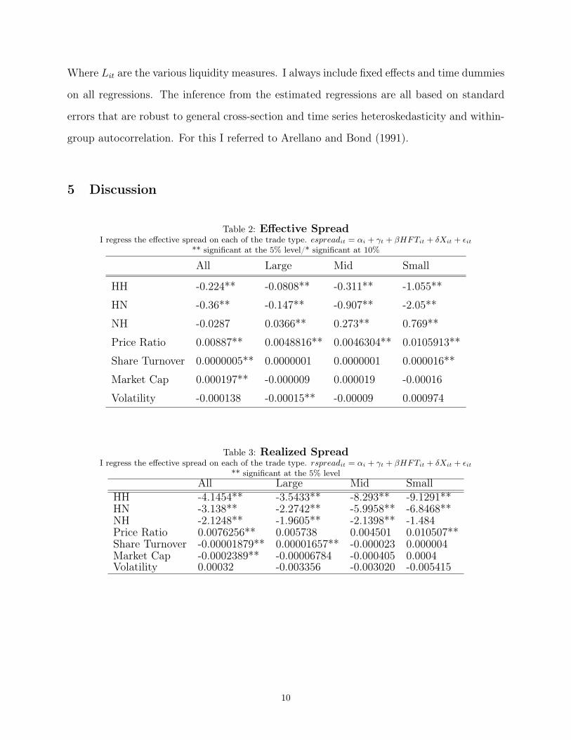
Where Lit are the various liquidity measures. I always include fixed effects and time dummies

on all regressions. The inference from the estimated regressions are all based on standard

errors that are robust to general cross-section and time series heteroskedasticity and within-

group autocorrelation. For this I referred to Arellano and Bond (1991).

5 Discussion

Table 2: Effective SpreadI regress the effective spread on each of the trade type. espreadit = αi + γt + βHFTit + δXit + εit

** significant at the 5% level/* significant at 10%

All Large Mid Small

HH -0.224** -0.0808** -0.311** -1.055**

HN -0.36** -0.147** -0.907** -2.05**

NH -0.0287 0.0366** 0.273** 0.769**

Price Ratio 0.00887** 0.0048816** 0.0046304** 0.0105913**

Share Turnover 0.0000005** 0.0000001 0.0000001 0.000016**

Market Cap 0.000197** -0.000009 0.000019 -0.00016

Volatility -0.000138 -0.00015** -0.00009 0.000974

Table 3: Realized SpreadI regress the effective spread on each of the trade type. rspreadit = αi + γt + βHFTit + δXit + εit

** significant at the 5% levelAll Large Mid Small

HH -4.1454** -3.5433** -8.293** -9.1291**HN -3.138** -2.2742** -5.9958** -6.8468**NH -2.1248** -1.9605** -2.1398** -1.484Price Ratio 0.0076256** 0.005738 0.004501 0.010507**Share Turnover -0.00001879** 0.00001657** -0.000023 0.000004Market Cap -0.0002389** -0.00006784 -0.000405 0.0004Volatility 0.00032 -0.003356 -0.003020 -0.005415

10

Table 4: Adverse SelectionI regress the effective spread on each of the trade type. AdversSelectionit = αi + γt + βHFTit + δXit + εit

** significant at the 5% levelAll Large Mid Small

HH 3.9357** 3.4662** 7.9792** 8.10035**HN 2.79** 2.128** 5.0891** 4.8863**NH 2.10** 1.9979** 2.4097** 2.1904Price Ratio 0.00109982 -0.00076123 0.0001335 0.00051Share Turnover -0.000018** -0.00001644** -0.0000229 0.00001267Market Cap -0.0000449 -0.000054 -0.00038678 -0.0001544Volatility -0.0000455 -0.00350387 -0.00311269 0.0064813

The results found in this study show that overall effective spreads decrease with HFT trading.

However, one important exception is noted in the results. I find that when HFTs are liquidity

suppliers to non-HFTs, spreads are wider. This implies that HFTs are imposing a higher

cost of immediacy on non-HFTs.

As explained previously in this paper, to analyze the source of the change in the effective

spread I decompose the effective spread measure into the realized spread and the price impact

following Glosten (1987). This decomposition will allow us to determine if the source of the

decrease is a result of less revenue for liquidity suppliers (a decrease in the realized spread),

decrease in losses due to more informed liquidity demanders (a decrease in adverse selection)

or a combination of both. The spread is the cost of immediacy. Liquidity suppliers benefit

from wider spreads since it generates larger revenues from providing immediacy to the more

desperate liquidity seekers. Through their low latency feature and technology advantages,

HFTs are able to increase liquidity supplying revenue when providing liquidity to nHFT.

This is true for all strata of market capitalization. However, the impact is larger for the

smaller cap group. For example, the results on table 2 show that for mid cap effective

spreads increase by 0.273 basis points when HFT supply liquidity to nHFT. The outcome

is significantly different when nHFT supplies liquidity to nHFT. In this case, the effective

spread decreases by 0.907 basis points. These results are consistent with the literature.

Hendershott et. al. (2013) , Biais, et. al. (2011), and Jovanovic Menkveld (2012) all arrive

at similar conclusions.

11

The natural question is what is the source of the liquidity increase when HFT supply liquid-

ity to nHFT. To answer this query, we need to analyze the decomposed spread measure. The

realized spread shows the revenue to liquidity suppliers. An increase in the realized spread

implies an increase in gross revenues to liquidity suppliers. From table 3 we see that the

revenue to liquidity suppliers decreases for all market capitalization and trader type combi-

nation. However, the decrease is smaller when HFTs are the liquidity suppliers. A possible

reason for this is that HFTs are better able to react and pick off the slower non HFTs. To

test this hypothesis, I conduct the same regression with a 60 second realized spread and

adverse selection. If my contention is correct, then we would expect that the adverse selec-

tion coefficients for HFT liquidity demanders are much smaller after 60 seconds of reaction

time. In addition, the difference between the adverse selection cost imposed by HFT liquid-

ity demanders and Non HFT liquidity demanders should be smaller. This is because of the

longer reaction time allowed to the non HFT. The results suggest that this is the case. The

results presented on Table 7 show that the adverse selection costs are smaller for the HFT

liquidity demander as compared to the 5 second adverse selection. For example, Table 7

shows that the 60 second adverse selection cost imposed by HFT liquidity demanders for the

entire sample is 1.9675 basis points. Compared to the result on Table 4 which shows a 2.79

basis point result obtained with the 5 second time interval. The longer time interval results

show a drop in adverse selection of 29.35%. A similar result is noted with large cap stocks

which has a drop of approximately 40%. This illustrates the waning effect of the HFT low

latency advantage as time elapses. Thus, giving slower traders more reaction time.

Table 5: Realized Spread 60 SecondsAll Large Mid Small

HH -1.30 -0.7166 -11.472** 2.9329HN -2.334** -1.4625* -6.559** 1.4147NH -1.817 -1.5974* -3.725* 4.5143

Price Ratio -0.0649821 0.05968319 0.325032 -0.217365Share Turnover 0.0000105 0.0000094 0.0000763 -0.00017882Market Cap -0.0014851 0.00014828 0.026339 -0.00614276Volatility 0.0299176 0.0265976 0.0394581 0.02609065

12

Table 6: Adverse Selection 60 SecondsAll Large Mid Small

HH 1.117 0.6661 11.2688** 2.231HN 1.9675** 1.279** 5.632** -3.064NH 1.9184** 1.6921** 4.3891* -3.919

Price Ratio 0.05166904 -0.0575718 -0.32574517 0.2363954Share Turnover -0.00001051 -0.00001 -0.00007542 0.0001948Market Cap 0.0014455 -0.00009976 -0.02495893 0.0086205Volatility -0.03084771 -0.0270517 -0.0406799 -0.0328586

Crisis Week

During the trading week of September 15th 2008 - September 19th, 2008, the stock market

saw one of its most volatile weeks in history. On Monday September 15th, 2008, equity

markets woke up to the news that Lehman Brothers declared bankruptcy, Merrill Lynch had

sold to Bank of America and that financial markets across the world were stifled with fear

and uncertainty. The day progressively worsen as news of the fate of the insurance giant

AIG remained at the mercy of US policy makers. That day the NASDAQ dropped 3.6%, the

biggest single day drop since September 11th, 2001. The remainder of the week was riddled

with uncertainty as policy makers and the Federal Reserve struggled to find a solution to

ease the financial market turmoil. To study the impact of HFT on liquidity during this time

of peril, I conduct the same analysis with a subset of the data containing the crisis week of

September of 2008.

Table 7: Descriptive Statistics Crisis WeekThis table presents summary statistics on 120 stocks traded on the NASDAQ for the crisis week of September 15- 19, 2008.Each stock is classified in one of three market capitalization categories: large, medium, or small. The unbalanced panel containsobservations for 5 trading days. The price ratio is estimated by 1 divided by the price. Volatility is calculated by the standarddeviation of the daily stock returns from open to close.

Variable Units Source All Large Medium SmallMarket Capitalization $ Billions CRSP 65.683 75 2.08 0.629Price $ CRSP 47.56 50.97 26.13 18.37Price Ratio % NASDAQ 3.465 3.122 5.396 7.47587Effective Spread bps NASDAQ 2.9588 2.2279 6.2843 12.87Realized Spread 5 seconds bps NASDAQ -6.168 -1.369 -47.13 -6.99Adverse Selection bps NASDAQ 9.128 3.648 53.418 19.864Volatility % CRSP 79.70 76.57 85.77 94.24

13

Table 8: Effective Spread Crisis WeekI regress the effective spread on each of the trade type. espreadit = αi + γt + βHFTit + δXit + εit

** significant at the 5% level

All Large Mid Small

HH -0.147** -0.06064** -0.3663* -0.5373

HN -0.412** -0.182** -1.1516** -2.3173**

NH 0.0912* 0.09464** 0.5967** 1.6143**

Price Ratio -0.004552 0.00281887* 0.0101957* -0.0047498

Share Turnover 0.0000003 -0.0000006* 0.000001 0.00004742**

Market Cap 0.0002292 -0.00008331 0.00194816** 0.00023417

Volatility -0.0009474** -0.00046722** -0.00119371** -0.00737478**

Table 9: Realized Spread Crisis WeekI regress the effective spread on each of the trade type. rspreadit = αi + γt + βHFTit + δXit + εit

** significant at the 5% level

All Large Mid Small

HH -2.1588** -1.11162 -10.2182** -8.8547HN -3.1579** -1.8682** -5.8542** -5.4641*NH -2.1621** -1.6857** -0.7315 -0.5135Price Ratio -0.0443267 0.0602366 0.18532563 -0.124575Share Turnover 0.00001386 0.00001456 0.00003594 -0.00016Market Cap -0.00094643 -0.00015116 0.01739087 0.00033185Volatility 0.02808367 0.024453 0.0487004 0.03098856

Table 10: Adverse Selection Crisis WeekI regress the effective spread on each of the trade type. AdversSelectionit = αi + γt + βHFTit + δXit + εit

** significant at the 5% levelAll Large Mid Small

HH 2.0007* 1.0646 9.9976** 8.2322HN 2.7325** 1.6836** 4.9111** 3.6339NH 2.2473** 1.7807** 1.3918 1.3637Price Ratio 0.0380618 -0.0580315 -0.187869 0.1456Share Turnover -0.00001361 -0.00001516 -0.00003509 0.00018606Market Cap 0.00116214 0.00020194 -0.01616722 0.0019936Volatility -0.0291 -0.02490697 -0.04999496 -0.03854794

The results on table 8 show that effective spreads are narrower when non HFT are liquidity

suppliers but wider when HFT are the providers of liquidity. For example, the effective

spread when a non-HFT supplies liquidity to an HFT is -0.182. However, when a HFT

14

supplies liquidity to a non-HFT, the effective spread is 0.09465. Thus, HFT are able to

consistently make positive revenues from liquidity provision. In addition, in comparison to

the full data sample results, the revenues from HFT liquidity provision in large cap stocks

were 167% higher during the crisis week. Whereas for non-HFTs liquidity provision revenues

where 24% lower. The same pattern persists for mid and small cap stocks. This illustrates

that during this time of high uncertainty, HFTs were able to increase their liquidity supplying

revenue whereas, the non HFT saw a further decrease.

To understand the source of the differences in liquidity supplying revenue between the HFTs

and non HFTs, we need to examine the realized spreads and adverse selection. There are two

possible reasons why these differences exist. First, it could be that, during the crisis week, as

the market was constantly shocked with new information, it increased the number of HFT

opportunities to adversely select the non HFT via the HFT speed advantages. Second, it

could be that in such uncertain times, the value of liquidity increases given that panic sales

become more common and liquidity becomes more valuable. When comparing the differences

in realized spreads from the full sample and the crisis week we see that most of the increase

in the spread was driven by realized spreads. Therefore, the value of liquidity became dear

during the crisis. This result is surprising since I expected that the numerous information

shocks during the crisis would lead to ample opportunities for the HFTs to take advantage

of their fast speed and pick-off non-HFTs. However, these results are consistent with the

theoretical model developed in Hoffmann (2014). In this paper, the author shows that in

periods of high volatility, slower traders submit limit orders that have low probabilities of

execution. Therefore, reducing the risk of getting adversely selected by fast traders. Non-

HFTs have a larger risk of being picked off when the trader is not sufficiently fast to react

to new information. As a result, market order traders sometimes obtain rents in addition to

their limit order value because favorable price movements render outstanding limit orders

stale. This becomes more common in environments of high volatility and causes liquidity

provision to became more risky. Consequentially, limit order traders will set their prices

further away from the market price making spreads larger. Comparing the results presented

15

in table 2 with the results in table 8 we see that this is the case when HFT supply liquidity

to non-HFTs and vice-versa.

6 Conclusion

Improvements in technology have revolutionized how financial assets are traded and how

financial markets function. Today, a large number of trades are conducted using super fast

computers that are able to react and trade in split seconds. Given these innovations, I

examine the role of HFT on market liquidity. To do this analysis, I used a proprietary data

set from the NASDAQ OMX that identifies the trading activity from 26 high frequency

trading firms. Overall HFTs increase liquidity in the equity market I analyzed. I find that

effective spreads narrow when HFTs supply liquidity to a nHFT. However, the effective

spreads widen when nHFTs supply liquidity to an HFT. These results indicate that HFTs

are able to gain from liquidity provision whereas nHFT are not able to. By examining the

decomposed spreads, I find that the source of most of the differences in the results seem to

stem from increasing adverse selection costs. Given the speed advantage of HFTs, they are

able to take pick-off the slower traders. This imposes an adverse selection cost on nHFTs who

are not able to react and cancel stale limit orders. During the crisis week of 2008, compared

to the full sample, the effective spreads were even wider when HFTs supplied liquidity. In

this case, the source of the increase was from increase liquidity provision revenues.

16

References

• Arellano Manuel, Stephen Bond, Some Tests of Specification for Panel Data: Monte Carlo Evidenceand an Application to Employment Equations, The Review of Economic Studies, Volume 58, Issue 2,April 1991, Pages 277–297, https://doi.org/10.2307/2297968

• Benos, Evangelos & Sagade, Satchit. (2012). High-Frequency Trading Behaviour and Its Impact onMarket Quality: Evidence from the UK Equity Market. SSRN Electronic Journal. 10.2139/ssrn.2184302.

• Bershova, Nataliya, Dmitry Rakhlin, 2013, High Frequency Trading and Long-Term Investors: A Viewfrom the Buy-Side, Journal of Investment Strategies, Volume 2, Issue 2, Pages 25-69.

• Biais, Bruno and Foucault, Thierry and Moinas, Sophie, Equilibrium Fast Trading, Journal of FinancialEconomics, 116, 292-313, 2015.

• Bogaard, Jonathan, Terence Hendershott and Ryan Riordan, 2013, High Frequency Trading and PriceDiscovery, The Review of Financial Studies, Volume 27, Issue 8, Pages 2267–2306.

• Carrion, Allen 2013. Very Fast Money: High-Frequency Trading on the NASDAQ. Journal of FinancialMarkets 16. 680-711.

• Glosten, Lawrence R. , 1987, Components of the bid ask spread and the statistical properties oftransaction prices, Journal of Finance, 1293-1307.

• Hagstromer Bjorn, Nordern Lars. 2013. The Diversity of High Frequency Traders. Journal of FinancialMarkets Volume 16, Issue 4, Pages 741-770.

• Hendershott Terrence, Jones Charles, Albert Menkveld, 2011, Does Algorithmic Trading Improve Liq-uidity? The Journal of Finance, volume 66, Issue 1, Pages 1-33.

• Hoffmann Peter, A Dynamic Limit Order Market with Fast and Slow Traders. 2015. Journal ofFinancial Economics 113 (1), 156-169.

• Jovanovic, Boyan and Menkveld, Albert J., Middlemen in Limit Order Markets (2016). Available atSSRN: https://ssrn.com/abstract=1624329 or http://dx.doi.org/10.2139/ssrn.1624329

• Kirilenko, Andrei, Albert S. Kyle, Mehrdad Samadi, Tugkan Tuzun, 2011, The Flash Crash: TheImpact of High Frequency Trading on an Electronic Market. The Journal of Finance, Volume 72, Issue3, Pages 967-998.

• Hirschey, Nicholas. (2020). Do High-Frequency Traders Anticipate Buying and Selling Pressure?.Management Science. 67. 10.1287/mnsc.2020.3608.

• Ye, Mao & Yao, Chen & Gai, Jiading. (2012). The Externalities of High Frequency Trading. SSRNElectronic Journal. 10.2139/ssrn.2066839.

• Gao, Cheng & Mizrach, Bruce. (2013). High Frequency Trading in the Equity Markets During USTreasury POMO. SSRN Electronic Journal. 10.2139/ssrn.2294038.

• Lee, Ready, 1991, Inferiring Trade Direction from Intraday Data. The Journal of Finance, Volume 46,Issue 2, Pages 733-748.

• Malinova, Katya & Park, Andreas & Riordan, Ryan. (2012). Do Retail Traders Suffer from HighFrequency Traders?. Available at SSRN 2183806. 10.2139/ssrn.2183806.

• Tong, Lin. (2013). A Blessing or a Curse? The Impact of High Frequency Trading on InstitutionalInvestors. SSRN Electronic Journal. 10.2139/ssrn.2330053.

• Zhang Sarah, Ryan Riordan, 2011, Technology and Market Quality: The Case of High-FrequencyTrading, ECIS 2011 Proceedings, Paper 95.

• Zhang, S. Sarah. (2012). Need for Speed – An Empirical Analysis of Hard and Soft Information in aHigh Frequency World. SSRN Electronic Journal. 10.2139/ssrn.2136687.

17