Faculdade de Economia

da Universidade de Coimbra

Grupo de Estudos Monetários e Financeiros

(GEMF) Av. Dias da Silva, 165 – 3004-512 COIMBRA,

PORTUGAL

gemf@fe.uc.pt http://www.uc.pt/feuc/gemf

JOÃO BRAZ PINTO & JOÃO SOUSA ANDRADE

A Monetary Analysis of the Liquidity Trap

ESTUDOS DO GEMF N.º 06 2015

A Monetary Analysis of the Liquidity Trap

João Braz Pinto (a)

João Sousa Andrade (b)

(a) Deloitte Touche Tohmatsu Limited (Portugal), brazpinto.joao@gmail.com

(b) Corresponding author. GEMF, FEUC – University of Coimbra, jasa@fe.uc.pt

1

A Monetary Analysis of the Liquidity Trap

Abstract

Keynes has emphasized a particular situation in which the liquidity preference becomes

absolute, leading to monetary policy ineffectiveness: the near zero nominal rate of

interest does not allow negative values of the real interest rate. This situation is termed

liquidity trap (LT) and although popularized by the IS-LM Hicks-Hansen framework it

was authored by Robertson. It was also elected as the Keynesian case against the

classical one. In 1998 Krugman recovered the name by applying it to the Japanese

episode of the 1990's. The “lowflation” environment in USA and Europe brought again

the LT to the forefront. The quantitative easing monetary policy was followed in Japan

and is now applied in the USA and EMU as a solution to overcome the LT. But the LT

has been erroneously considered as a money demand problem and at the same time

denied as a “banking problem” in the words of Krugman. We contend that the current

situation should be interpreted as a “banking problem” that impedes the transformation

of the monetary base into money supply. In order to prove our thesis we study the

behavior of the USA money multiplier and the income velocity of money before the

beginning of the current crisis and during the crisis and by forecasting and estimating a

VAR and a VECM model we compare the normal situation of monetary policy

efficiency with the situation of LT monetary policy inefficiency.

JEL: E12, E3, E4, E51 and E6

Keywords: Liquidity Trap, Money Supply, Monetary Base Multiplier, ARIMA, VAR

and VECM models.

2

“But do not be reluctant to soil your hands, as you call it. I think it is most important. The specialist in

the manufacture of models will not be successful unless he is constantly correcting his judgment by

intimate and messy acquaintance with the facts to which his model has to be applied.” Keynes (1973),

p.300, Letter to Roy Harrod 10th July 1938.

1. Introduction

Until Krugman’s alarm, Krugman (1998), liquidity trap (LT) was a concept related to

the old Keynesianism and a curiosity in the USA history of monetary policy. The current

new situation in the USA and EU has caused a regained interest both historical and

theoretical about this phenomenon. We begin our paper (section 2) by recalling the

Keynesian definition of LT (2.1), its origin and critics to the concept. In the second sub-

section (2.2) the current LT definition is discussed as well as its implication. In the third

sub-section (2.3) we briefly point out several LT episodes with the objective to show

that LT is not a curiosity emanating from the minds of some creative economists. This

section also addresses the issue of how to get out of the LT vicious circle (2.4). Our

thesis about LT is presented in the end of this section (2.5) and we confirm it for the

USA in the empirical part of this paper (section 3). In this last section, after data

description (3.1), we study the behavior of the income velocity of money and the money

multiplier and with the help of a VAR and a VECM model we confirm our thesis about

the LT phenomenon (3.2). Finally we conclude (section 4).

2. A Reassessment of the LT Literature

2.1 A Keynesian definition of Liquidity Trap

Keynes (1936) has suggested the expression of absolute liquidity-preference

(p.191) to the situation we know nowadays as Liquidity Trap (LT). Tobin (1947) used

the expression “Keynesian impasse” (p.128) to express the same situation. We owe the

current term LT to Robertson (1940) p.34 and p.36 even if Hicks (1937) p.56 knew the

expression that was subsequently popularized by Hansen (1953), Sutch (2009).

Robertson proposed the expression to illustrate the consequences of a money demand

negatively sloped on the saving-investment process, Boianovsky (2003). The standard

Hicks-Modigliani-Hansen unemployment equilibrium model, Patinkin (1974), became

the source for the LT explanation based on the assumption of Keynesian interest rate

regressive expectations. The situation of a LT explained in terms of term structure of

interest rates proposed by Keynes and accepted by Hicks, was replaced by the idea that

3

the floor of the long run interest rate doesn’t depend on uncertainty, Kaldor (1939) and

Robinson (1951).

The LT was the main reason for the role ascribed by macroeconomic textbooks

of the 60’s to fiscal policy by identifying a “Keynesian case”, Modigliani (1944), p.561,

where “nobody will be willing to hold nonphysical assets except in the form of money”,

p.53. And as a consequence: “(a) any increase in the supply of money to hold now fails

to affect the rate of interest”, p.55. The General Theory (GT) was consequently

conceived as “the Economics of Depression”, Hicks (1937), p.155. The Bordo and

Schwartz (2003) observation that Modigliani (1944) viewed Keynes “absolute liquidity

preference as a curiosity and not the true hallmark of the Keynesian model” (p.221)

doesn’t express Modigliani thinking.

The refusal of the LT came from Patinkin (1974) that defends against the

conventional IS-LM model explanation of sustainable less than full-employment an

alternative one based on the GT, “generated by the fact that the rate of interest falls too

slowly in relation to the marginal efficiency of capital” (italics in the original, p.9). The

refusal comes also from Brunner and Meltzer (1968) two well-known representatives

of the monetarist thinking. These authors considered what they call different types of

LP: “Traps have been said to affect interest rates, the bank’s demand for excess reserves,

the public’s supply of loans or commercial banks, and the public’s demand for money”,

p.2. They correctly reoriented the discussion towards the transmission mechanisms of

monetary policy but they deny the ineffectiveness of monetary policy and so they also

deny the existence of the different kinds of traps, p.28. The authors write that “some

form of a trap had existed”, p.1, nevertheless they cite the famous p. 207 of Keynes

(1936) as a reference for its (non) existence, “I know of no example of it hitherto”, just

the opposite.

This hypothesis was subject to both theoretical and empirical critics. Haberler

(1937) and Pigou (1943) argued that deflation that characterized the LT hypothesis leads

to an increase in agents’ real income (a shift to the right of the IS curve) which would

be sufficient for economic recovery starting. This hypothesis was referred to as “Pigou

effect”. Monetarists like Friedman (1956) and Brunner and Meltzer (1968) argued that

the demand for liquidity would never become absolute and therefore monetary policy

1 The complete phrase is “This situation that plays such an important role in Keynes's General Theory

will be referred to as the `”Keynesian case”.

4

would remain effective if unconventional policies, that Friedman called “money gift”,

were adopted. Those policies consisted in establishing a higher monetary base growth

rate target or diversifying open market securities purchases with special focus on

longer-term maturities.

Since then a long period of time elapsed during which LT stayed dormant. It

was the time of Jean Fourastié’ trente glorieuses, the growing inflation of the 60’s with

the eclipse of the Phillips Curve, and the rational expectations revolution of the 70’s led

to the limbo not only the LT framework of analysis but also most of the Keynesian ideas

about over saving and deficient aggregate demand. We have “thrown out the baby with

the bath water” until the seminal article by Krugman (1998).

2.2 Current definitions of LT

In the framework of the IS-LM model, the phenomenon of LT is interpreted as

a situation of perfect substitutability of money and bonds at a (near-)zero short-term

nominal interest rate and so this irreducible interest floor becomes a binding constraint

making ineffective traditional procedures of monetary policy, Krugman (1998), Buiter

and Panigirtzoglou (1999), Benhabib, Schmitt-Grohé and Uribe (2002), Auerbach and

Obstfeld (2004), Hanes (2006), Svensson (2006), Eggertsson (2008), Sutch (2009), and

Rhodes (2011). Additionally, the Central bankers’ reputation for maintaining a stable

reduced inflation rate is also an important factor in current times to push interest rates

to near zero values Sumner (2002).

Buiter and Panigirtzoglou (1999) call LT “an inefficient equilibrium” and

Blinder (2000) comparing it with zero gravity or near absolute zero temperature writes

that “it may indeed be a new world” and Pollin (2012) stresses the specific environment

of high unemployment, high inequality, household wealth collapse and fiscal austerity

policies accompanying the LT. This is not far from what Modigliani (1944) defines as

the “Keynesian case” (P.56) or Hicks (1937) the “Economics of Depression” (p.155)

when the LM curve is horizontal.

The majority of the LT interpretations are addressed in terms of money demand

behavior. The problem of money supply is rarely taken into consideration and when it

occurs it is exclusively confined to the monetary base behavior. In Svensson (2003) the

confusion between monetary base (MB) and money supply effects is notorious, see

p.147. Krugman (1998) explicitly says that “base and bonds are viewed by the private

sector as perfect substitutes”, p.141. This may be true for banks but obviously not for

5

the “private sector”. So monetary policy is ineffective due to the behavior of money

demand. Some authors look at the MB but do not go further, e.g., Brunner and Meltzer

(1968) give another interpretation for monetary policy ineffectiveness, “the banks

desired to hold excess reserves and were unwilling to lend”, p.12, but they dismissed

that explanation in the absence of evidence supporting it as Sumner (2002) also did. A

similar interpretation is given too by Svensson (1999) and Svensson (2003) who claim

that the increase in the MB beyond the satiation point is ineffective on nominal and real

prices and quantities. Krugman (1998) recognizes the impossibility of increasing

“monetary aggregates” although the MB increment, he is categorical pointing out that

the essential problem does not lie in the banking sector, p.140, since the solution to the

problem is the creation of inflation expectations. But he does not explain how those

expectations can be effective in the absence of money supply growth. Pollin (2012)

shows that at least for the current crisis there is no satiation level for the MB in the USA

and so the problem lies on the transformation of the MB on money supply. And without

an increase in the money supply we cannot expect the reduction in longer interest rates

that will affect consumption and investment, Svensson (2003).

For Eggertsson and Woodford (2003) in a LT situation money demand is less

than money supply. We don’t agree with this thesis because we should take in

consideration the money demand for hoarding conducing to idle money balances and

the absence of bank credit reducing the money supply. Rhodes (2011) prefers the

expression “liquidity sump” where individuals want to convert income flows in excess

of basic income into money (liquid assets). If this portrays the current LT situation then

the money supply will be growing and this does not happen.

What are the consequences of the usual definition? Monetary policy is

ineffective to achieve full-employment or to reverse the downward slide in prices under

a LT context, Benhabib, Schmitt-Grohé and Uribe (2002)2. Auerbach and Obstfeld

(2004), Eggertsson (2005), Eggertsson (2008) are supportive to the idea that even in a

LT, large-scale open market operations are a powerful instrument for fiscal policy.

Bernanke (2000), Orphanides and Wieland (2000) and Pollin (2012) recommended

solutions to change the rigidity of high values of longer rates of interest in a LT.

The IS-LM model with the independence of the two curves is not an appropriate

framework for that proposal. Nevertheless the door was opened for the fiscal channel

2 We have no pretension of being exhaustive.

6

at the end of Keynes’ most cited passage, p.207, “Moreover, if such a situation were to

arise, it would mean that the public authority itself could borrow through the banking

system on an unlimited scale ...”.

2.3 LT episodes

Krugman (1998) seminal paper is responsible for the recent interest on LT

episodes. The ECONLIT records 36 articles until 1997 and 162 since 1999 until June

2014. Besides Krugman, other authors such as Auerbach and Obstfeld (2004),

Shirakawa (2002), Bernanke (2000), Eggertsson and Woodford (2003), Svensson

(2006) deserve to be mentioned due to their analysis of the LT episode - Japan in the

90’s. And Hanes (2006) and Eggertsson (2008) are good references for the early' 1930s

in the USA (1933).

The Fisherian explanation, Fisher (1933), about the Great Depression relies on

debt deflation. It is a very appealing explanation that envisages LT episodes as a process

that may not return to equilibrium. More specifically, it explains why the dynamics of

deficient or stagnant global demand and money supply is perpetuated in a vicious cycle

of decreasing prices – increasing debt value – and decreasing global demand. This

explanation was taken to explain Japan' 1990, Koo (2009) and Eggertsson and Krugman

(2012) and is also presented in Svensson (2003).

In our opinion, what we have now are different episodes of massive creation of

high power money by central banks. These experiences are known by the term

“quantitative easing” (QE) and they were applied first in the early 2000s in Japan and

then after the beginning of the current crisis (2007) in the United States, United

Kingdom, Japan, and the Euro Area, Fawley and Neely (2013).

2.4 How to get out of the vicious circle of LT

Buiter and Panigirtzoglou (1999) considerer that the question about LT is not

how to eliminate it but how to avoid it3. But this position does not eliminate the need

to put an end to a LT situation. In a LT the anemic aggregate demand is negatively

influenced by household deleveraging and must be compensated or reversed by

unconstrained agents, Mian and Sufi (2010), Guerrieri and Lorenzoni (2011), Hall

(2011), Eggertsson and Krugman (2012) and Korinek and Simsek (2013).

3 “Targeting a higher rate of inflation after you are caught in the trap would be like pushing toothpaste

back into the tube” (p17).

7

The traditional Keynesian policy proposal to eliminate the LT was based on the

displacement to the right of the IS curve by means of fiscal policy stimulus. This was

the approach justifying the “american fiscalism” position. The idea of fiscal stimulus

remains but nowadays mostly through future prices increase and consequently by

changing the intertemporal budget constraint of governments, Benhabib, Schmitt-

Grohé and Uribe (2002), Eggertsson (2008). Another kind of policy is to increase the

money supply choosing a money growth targeting that will be responsible for inflation

growth and so will change the intertemporal budget constraint of private agents as well

as government Krugman (1998) and Benhabib, Schmitt-Grohé and Uribe (2002). These

proposals are usually based on government’s function of spender of last resort. In this

case, this monetary strategy is the other face of the fiscal policy and in the limit “it is

government debt that determines the price level” Eggertsson (2003), p.5. Burgert and

Schmidt (2013) shows that the efficiency of this policy depends on the government debt

level. The most radical proposition comes from Cochrane (2013), following which the

fiscal stimulus should be regarded as “totally useless (...) government spending”4, p.10,

or in the words of Krugman (1998), government must “commit to being irresponsible”.

The effects of increasing government spending corresponds to one of the

particularities of the LT: what in normal times will reduce the natural level of output

will in a LT increase equilibrium employment, Eggertsson (2008), and so government

spending becomes self-financing, tax revenues will increase enough to pay for higher

spending, Erceg and Lindé (2014).

Let us now focus on the money supply side of the LT. We consider that we have

two problems in terms of money supply. The first problem is the velocity of money

decrease. The second one results from the fact that an increase in money supply in our

credit money economy is the outcome of banking anticipated solvable credit demand.

The first problem is very similar to the situation of over-saving considered by Keynes

that has lead this author to cite Silvio Gesell in the GT. Gesell (1916) proposed a tax on

currency, “one-thousandth of its face value weekly, or about 5% annually”, p.123, to

increase the velocity of money in order to stabilize the general level of prices. The

increase in money velocity will attenuate the decrease in aggregate demand in a LT,

4 Some suggestive examples “hiring people to dig ditches and fill them up or construct defenses against

imaginary alien invasions, to use two classic examples. It also can represent destruction of capital or

technological regress — throwing away ATM machines to employ bank tellers, idling bulldozers to

employ people with shovels, or even spoons, breaking glass or welcoming hurricanes, to use classic

examples.”

8

Buiter and Panigirtzoglou (1999). The second one is reflected on the very reduced value

of the money multiplier and could be solved by “an excess reserve tax”, Edlin and Jaffee

(2009) and Pollin (2012) or the imposition of a maximum reserve level Dasgupta

(2009)5.

Demand policies will be ineffective if individuals anticipate the return of the

inflation values prevailing during the LT period, Krugman (1998) and Rhodes (2011),

or if they anticipate that monetary authorities will continue to choose the interest rate

following a Taylor rule, Eggertsson and Woodford (2003). Both situations are the denial

of the idea that Central Banks can create the amount of money they wish. When

Bernanke (2000) has written that “(t)he monetary authorities can issue as much money

as they like”, p.5, we must read “money” as “base money” and not “money stock”.

A third alternative to eliminate the LT consists in a sustainable reduction of long-

term interest rates through the supply of reserves in exchange of foreign currency and

long-term government bonds, Hanes (2006). This effect may be achieved through loan-

guarantee programs (especially) to smaller firms, Pollin (2012), that will reduce their

risk premium. This effect to work out has to countervail the moral-hazard problem as

well as the inefficiency in the credit market that it will create. Following Orphanides

and Wieland (2000), to reduce long term interest rates it is sufficient a commitment by

the central banks on very low short term interest rates. Bernanke (2002) proposed an

operational procedure to guarantee high prices in unlimited quantity for future

government bonds. This alternative is denied by Svensson (2003) and Svensson (2006)

that points out that expectations of higher future price levels are more effective.

Svensson (2001), Svensson (2002) and Svensson (2006) proposed what he calls the

“Follproof Way” to eliminate the LT. This consists of a price-level increasing target

path, currency depreciation with currency peg and a zero interest rate until positive

results in price-level targets has been reached. But he regards the monetary base as a

sufficient condition to change expectations of prices increases what is a wrong

deduction during a LT episode because as mentioned above in a LT situation the money

supply does not reacts to increases in the monetary base.

2.5 Our Thesis

5 An example of this kind of measure is represented by ECB decisions on 5th June 2014 to reduce its

deposit facility interest rate from 0% to -0.10%, and on 4th September to -0.20% and also to remunerate

excess reserves at this rate.

9

The common vision bases the phenomenon of LT on the demand for money. We propose

to analyses it as a rupture in the money supply mechanism. The central problem is the

banking sector. Banks do not create money because they do not have reserves to do so

but instead they consider that there is no acceptable level of risk from bank credit

demand. The proposals to eliminate this situation based on the creation of inflation

expectations should be compatible with money supply targets and should be founded in

realistic forecasts of banking lending.

The current analysis of LT has some limitations that are a direct consequence of

the framework of analysis initially used - the IS-LM model. This model has two black

boxes (BB) in terms of monetary policy: (1) the oversimplification of the relationships

between the Central Bank (CB) and the banking system and (2) the neglect of the

relationships between banks and the non-banking sector, Dale and Haldane (1993). The

first BB leads to ignoring that the LM curve depends on the operational targeting of the

CB (refinancing interest rate or monetary base), Bofinger (2001), p.85-90, and to

assume that banks have a passive role in the transmission of monetary policy. In a LT

situation the chain represented by the monetary base multiplier is broken and so this

monetary transmission mechanism does not work. The second BB by ignoring the

banking credit demand ignores money creation, i.e. money supply. The LM curve

represents the equilibrium between the demand and supply of money. Money demand

is dependent on income6 and its value is always finite and so a LM curve represented

by a horizontal curve makes non-sense. An LM curve horizontal supposes an infinite

banking lending to the economy for an infinite value of the permanent income. The

derived idea of a near zero velocity of money in a LT situation is also incorrect.

We have by now a considerable period of an ex ante strategy for monetary

expansion, Fawley and Neely (2013), and we focus on the quantitative easing in the

U.S.A. The concept of QE refers to a set of unconventional monetary policy measures

related to changes in structure and/or balance sheet size of central banks and massive

asset purchases by introducing high power money in huge amounts seeking to facilitate

access to credit for non-financial agents. There are two historical episodes, identical in

shape but different in content, of the adoption of such policies: by the Bank of Japan

after the Japan’s Lost Decade and by the FED during the period following the 2007

Financial Crisis.

6 Current or permanent income or wealth. But for our main argument this is secondary.

10

The strategy adopted by the FED can be divided into two phases: the first,

beginning in 2008, was marked by an ad hoc approach centered on the left side of the

balance sheet (assets): purchase of longer maturities assets (Treasury notes and

Treasury bonds), regardless of the usual Treasury bills (maturity less than 1 year). The

objective was to promote monetary expansion by reducing the liquidity premium.

The second phase was characterized by operations on liabilities: the U.S. Treasury

resorted to loans beyond their needs depositing excess funds in their accounts with the

Fed. The action therefore focused on the reduction of the risk premium, which reveals

a paradigm shift in the FED action during the implementation of QE: at first the

financial crisis was seen as a problem of illiquidity and in a second moment the FED

adopted an approach to troubleshoot solvency of the financial sector and in this way the

objective was to increase the supply of credit to the non-financial sector of the economy.

In a LT episode banks have excess reserves but they don’t lend them. The

situation is not one of excess-demand for money but of a shortage of bank credit and so

the money supply is stagnant. As a consequence global demand is sluggish and inflation

expectations are not far away from zero, if not from negative values.

The problem in terms of diagnosis is on the rupture of the money multiplier and

in terms of the cure on the spender side of the economy. Government must borrow

money to spend it immediately and “conditions” must be offered to banks to lend money

to firms, even if this create a moral hazard problem.

The classical analysis of active/idle balances, Humphrey (1974) and Humphrey

(2004), is ignored nowadays. Let us return to this analysis. In a LT episode the level of

idle balances is growing and this is equivalent to an excess of money supply. The

Government could borrow these balances and spend them, even if this operation

increases the borrowing interest rate. Is this operation in contradiction with the classical

policy measure of reducing the interest rate to near-zero values? No, it is not. If idle

balances are transformed in active balances, the increase in global demand will

contribute to the money supply growth and the major problem in LT relies on the money

supply mechanism. Consequently, special emphasis should be accorded to the

proposition that follows, without no banking credit demand there will be no increasing

money supply.

3. Empirical Analysis

11

We first describe our database and make some descriptive analysis of the

variables of interest and then we test our thesis about the existence of LT for the USA

economy after 2008, following which LT is a banking problem and not a money demand

problem. The econometric study if conducted in two stages, (A) and (B). In the first

stage (A) we study the evolution of the income velocity of money and the money

multiplier. We compare the actual values during the financial crisis with forecasting

values obtained until its beginning. With this analysis we focus on two characteristics

of LT: the decline of the money velocity which is usual recognized but exaggerated and

the decline of the money multiplier that is almost always ignored. In the second stage

(B), we build and estimate two reduced money supply models (a VAR and a VECM) in

order to draw conclusions about the responses of the variables to shocks7. This will

enable us to evaluate the impact of money supply policies (such as QE) on the U.S

economy. We have divided the period of study (1959:01 to 2013:10) in a “normal

period” (1959:01 to 2008:03) and a “crisis period” (2008:04 to 2013:12), and the latter

one we associate to a possible LT period.

3.1 Data and descriptive analysis

The database is from FRED (Federal Reserve Bank of St. Louis) and contains monthly

values between 1959:01 and 2013:10. The variables are the output (LYR), the nominal

interest rate (R), the consumer price index (LP), the monetary base (LMB) and the

monetary aggregate (M1). All variables except the nominal interest rate, are in logs.

LYR refers to real GDP at 2009 prices in billions USD. This variable was converted

from quarterly to monthly data using the package “tempdisagg” for “R” software, Sax

and Steiner (2013). R is the Effective Federal Funds Rate, the actual values of the

operational target of the FED monetary policy. LP is a measure of monthly prices of a

set of goods and services purchased by consumers with 1982-84 as the base year. LMB

refers to the adjusted monetary base of the Federal Reserve of St. Louis. LM1 is the

narrow definition of money supply in the U.S. Lv measures the income velocity of

money (=LYR+LP-LM1), while Lm measures the money multiplier (=LM1-LMB).

We highlight in what follows the evolution and the relationship between two of

the crucial variables of our study the money supply (M1) and monetary base (MB).

Looking at their evolutions in Figure 1 and 2 we perceive after 2008 a great increase in

7 The shock value is equal to the standard deviation of the estimation for each variable.

12

the values of M1 and a huge MB growth. These evolutions hide a completely difference

picture in terms of the transmission mechanism of monetary policy. In Figure 3 we

represent in a scatter the relation between M1 and the MB and it exhibits a rupture in

the relationship after the beginning of the financial crisis.

Figure 1

Figure 2

0

500

1000

1500

2000

2500

1960 1970 1980 1990 2000 2010

M1

Money Supply

0

500

1000

1500

2000

2500

3000

3500

4000

1960 1970 1980 1990 2000 2010

BM

Monetary Base (St. Louis)

13

Figure 3

3.2 Econometric Analysis

We study now the evolution of the income velocity of money and the money

multiplier (A). In a LT the velocity of money, Lv, will tend to minimum values

corresponding to an increase in the amount of idle money. The following general ADL

(augmented distributed lags) model was investigated:

( ) ( )1t t t tLv = c + a L Lv + b L R + ε−

(1)

where a(L) and b(L) are lag polynomials with maximum order of 68. The model is on

Table 1.

Table 1. OLS, 1959:03-2008:03 (T = 589), for Lv HAC standard errors, bandwidth 6 (Bartlett kernel)

Coeff.

Const 0.0053* R²=0.999 AR1: F(1,584)= 0.139

R_1 0.0005*** σ=0.006 RESET: F(2, 583) = 1.864

Lv_1 1.2683*** F(3,585)=1324137

Lv_2 -0.2693**

Notes: author's calculations. The last statistics in the second column is a LM test for the null of all

coefficients beyond the constant. In the third column we have an AR1 LM test and a RESET with the

squared and third exponent.

As we see we have no problems of autocorrelation of the errors or model

misspecification. The coefficient of the interest rate is positive as expected. The forecast

for the period of crisis, considering a confidence interval of 90%, is shown in Figure 4.

8 For all estimated regressions we choose lags by the likelihood ratio criterion.

0

500

1000

1500

2000

2500

3000

0 500 1000 1500 2000 2500 3000 3500

M1

BM

M1 versus BM (with least squares fit)

Y = 297. + 0.617X

14

Figure 4 – Income velocity of money (M1)

The velocity of money fell far beyond what was expected from the previous

behavior, what can be interpreted as a situation of “excess money” because a substantial

part of the stock of money is inactive (the fall was 40% compared to the forecast value).

This evolution is in accordance with our representation of LT.

We consider that the normal transmission mechanism of monetary policy does

not work in a LT situation. The banking sector does not transform “high power money”

into money supply, money that circulates in the economy. This capacity of the banking

sector can be measured by the money multiplier. The ADL model for Lm is the

following:

( ) ( ) ( ) ( )1t t t t t tLm = c + a L Lm + b L R + c L LYR + d L LP + ε−

(2)

where the terms ( )a L , b( )L , c( )L and d( )L are lag polynomials. We continue to

consider the period prior to 2008:08 and the period post 2008:09. The Lm model

excludes LYR and LP and keeps R with a polynomial lag of order 5 and the dependent

variable has a polynomial lag order equal to 4. The estimated model is on Table 2.

Table 2. OLS, 1959:06-2008:08 (T = 591), for Lm

HAC standard errors, bandwidth 6 (Bartlett kernel)

Coeff.

Const -0.0004 R²=0.999 AR1: F(1,580)= 0.327

R_1 -0.0015*** σ=0.005 RESET: F(2, 579) = 2.058

R_2 -0.0003 F(9,581)=497137

R_3 0.0007

6.3

6.4

6.5

6.6

6.7

6.8

6.9

7

2000 2002 2004 2006 2008 2010 2012 2014

90 percent interval

Lv

forecast

15

R_4 -0.0004

R_5 0.0011**

Lm_1 0.945***

Lm_2 0.0104

Lm_3 0.1985***

Lm_4 -0.1543***

Notes: author's calculations. See notes on Table 1.

The sum of the coefficients associated with lagged Lm is approximately 1

(1.001), for a standard deviation of 0.0005. Again, we have no problems of

autocorrelation and misspecification. The dynamic forecasts of the money multiplier

for the crisis period, with the 90% confidence interval, is in Figure 4. The evolution of

Lm reflects a relative stability of the money multiplier, as was supported by monetarist’s

authors. The least we can say about the evolution of their values during the crisis is that

the fall was brutal (for instance in 2013:10 the difference between the actual and the

forecast value was 74%). In our opinion this is an essential characteristic of the LT.

Figure 5 – Money multiplier

At stage (B) we analyze the LT from the point of view of money supply. We

consider the following scenario: the Central Bank opts for a policy of money creation,

increasing the monetary base, but banks, either due to rearrangement of their assets or

to the reduction of their lending capabilities, do not increase the money supply. The

monetary policy is in this situation ineffective. To verify this hypothesis we propose a

reduced model in which the interaction between monetary base and money supply

-0.6

-0.5

-0.4

-0.3

-0.2

-0.1

0

0.1

0.2

0.3

0.4

2000 2002 2004 2006 2008 2010 2012 2014

90 percent interval

Lm

forecast

16

(LMB and LM1)9 variables are studied. The model is applied to the two sub-periods

previously defined. We analyze the effectiveness / ineffectiveness of monetary policy

with a VAR in a situation of LT through the comparison of the results from different

shocks in the two periods.

The order of the VAR for the first sub-period is 7 and for the second period is

3. Since both variables are first order integrated we’ve also applied the Johansen

cointegration test to see if we could have a long-run relationship between these two

variables. The lags chosen for the test correspond to those of the VAR model minus one

and we never retained any cointegration vector. For both sub-periods the Cholesky

decomposition was retained. With regard to the first sub-period no autocorrelation of

order 1 problems were detected. Tables 3 and 4 below contain the values of the variance

decomposition for LMB and LM1, respectively.

Table 3. Variance decomposition for LMB (VAR – 1st sub-period)

Period Standard error LMB LM1

1 0.004 100.00 0.00

12 0.022 97.71 2.29

24 0.036 95.26 4.74

36 0.047 93.19 6.81

Table 4. Variance decomposition for LM1 (VAR – 1st sub-period) Period Standard error LMB LM1

1 0.005 29.16 70.84

12 0.028 33.04 66.96

24 0.044 35.33 64.67

36 0.055 37.08 62.92

As can be seen LMB is mainly explained by itself (93%) while it explains 37%

of the variance of LM1. This model is stable, as the roots associated with the VAR lie

inside the unit circle (Figure 6).

Figure 6. Inverse of the VAR roots on the unit circle (VAR - 1st sub-period)

9 The variables were ranked in terms of proximity to the action of MA.

17

Figure 7. Money Supply and Money Demand Shocks (VAR - 1st sub-period)

We will identify a shock of LMB as a money supply shock and a shock of LM1

as a money demand shock (Figure 7.). A money supply shock causes, in the period up

to the present crisis, an increase in the money supply that stabilizes after almost a year.

A money demand shock has a much reduced effect on the monetary base and after 1

year is practically negligible. Thus, the role of monetary authorities through money

supply policy is clear and corresponds to what is expected theoretically. At the same

time we confirm the characteristic of exogeneity for the monetary aggregate M1.

We present now the second sub-period VAR. We continue to have no problems

of autocorrelation of order 1. The values of the decomposition of the variance of the

two variables are in Tables 5 and 6.

Table 5. Variance decomposition for LMB (VAR – 2nd sub-period)

Period Standard error LMB LM1

1 0.030 100.00 0.00

12 0.081 85.99 14.01

24 0.097 61.26 38.74

36 0.111 46.67 53.33

18

Table 6. Variance decomposition for LM1 (VAR – 2nd sub-period)

Period Standard error LMB LM1

1 0.014 1.23 98.77

12 0.048 2.44 97.56

24 0.071 1.23 98.77

36 0.088 0.86 99.14

We find a strong participation of LM1 in the variance of LMB (53%) reflecting

a strange effect in terms of monetary theory. Regarding the variance of LM1, LMB has

virtually no explanatory role unlike what happened in the first sub-period and LM1 is

explained almost by itself (99%). The model remains stable (Figure 8).

Figure 8. Inverse of the VAR roots on the unit circle (VAR - 2nd sub-period)

Figure 9. Money Supply and Money Demand Shocks (VAR – 2nd sub-period)

A shock of money supply quickly cancels its effects on LM1 and its effects can

never be taken as non-zero (Figure 9). In turn, money demand shocks significantly and

durably affect LMB. So contrary to what happened before the crisis, money supply

shocks don’t have a growth effect in money circulating in the economy. It can be

19

concluded that for the period under review, monetary policy based on money supply

shocks is ineffective in preventing the emergence of a situation of deflation.

Hoffman and Rasche (1996) marked a new route in monetary empirical research

with cointegration (C-I) monetary modeling. We propose a model with the rate of

interest, the monetary base and the income velocity of money (R, LMB and Lv). These

variables are I(1) by the usual ADF and KPSS tests. For the first sub-period the optimal

order of the VECM for the Johansen test is 6. We see (Table 7) that we cannot reject

the existence of 1 vector for C-I.

Table 7. Johansen Test: Lag order =6, 1959:07 – 2008:03, Unrestricted constant

Rank Trace test Lmax test Trace test (C)

0 55.28*** 43.09*** 55.28***

1 12.20 11.22 12.20

2 0.979 0.979 0.979

Notes: the last column refers to the trace test corrected for sample size (df=566).

The sign of the short-term adjustment coefficient (α) is negative and so the

process is stationary. As we have done below we retain the Cholesky decomposition to

obtain the variance decomposition and responses to shocks. For each of the VAR

equations associated with the VECM we do not have problems of auto-correlation. In

Tables 8, 9 and 10 we have the values of the decomposition of the variances and in

Figure 10 we have the inverse of the VAR roots inside the unit circle.

Table 8. Variance decomposition for R (VECM - 1st sub-period) Period Standard error R LMB Lv

1 0.405 100.00 0.00 0.0000

12 1.601 88.74 2.26 9.0021

24 2.068 83.52 4.35 12.1286

36 2.319 81.63 5.23 13.1393

Table 9. Variance decomposition for LMB (VECM – 1st sub-period)

Period Standard error R LMB Lv

1 0.004 0.17 99.83 0.00

12 0.021 3.68 96.17 0.15

24 0.033 2.42 97.46 0.12

36 0.043 1.57 98.32 0.11

Table 10. Variance decomposition for Lv (VECM – 1st sub-period)

Period Standard error R LMB Lv

20

1 0.006 0.88 17.31 81.81

12 0.036 39.53 6.80 53.67

24 0.059 41.16 3.92 53.67

36 0.077 42.32 2.79 54.89

Both R and LBM are mostly explained by themselves while R has a share of

42% in explaining Lv which corroborates the importance of the interest rate in the

transmission mechanism of monetary policy.

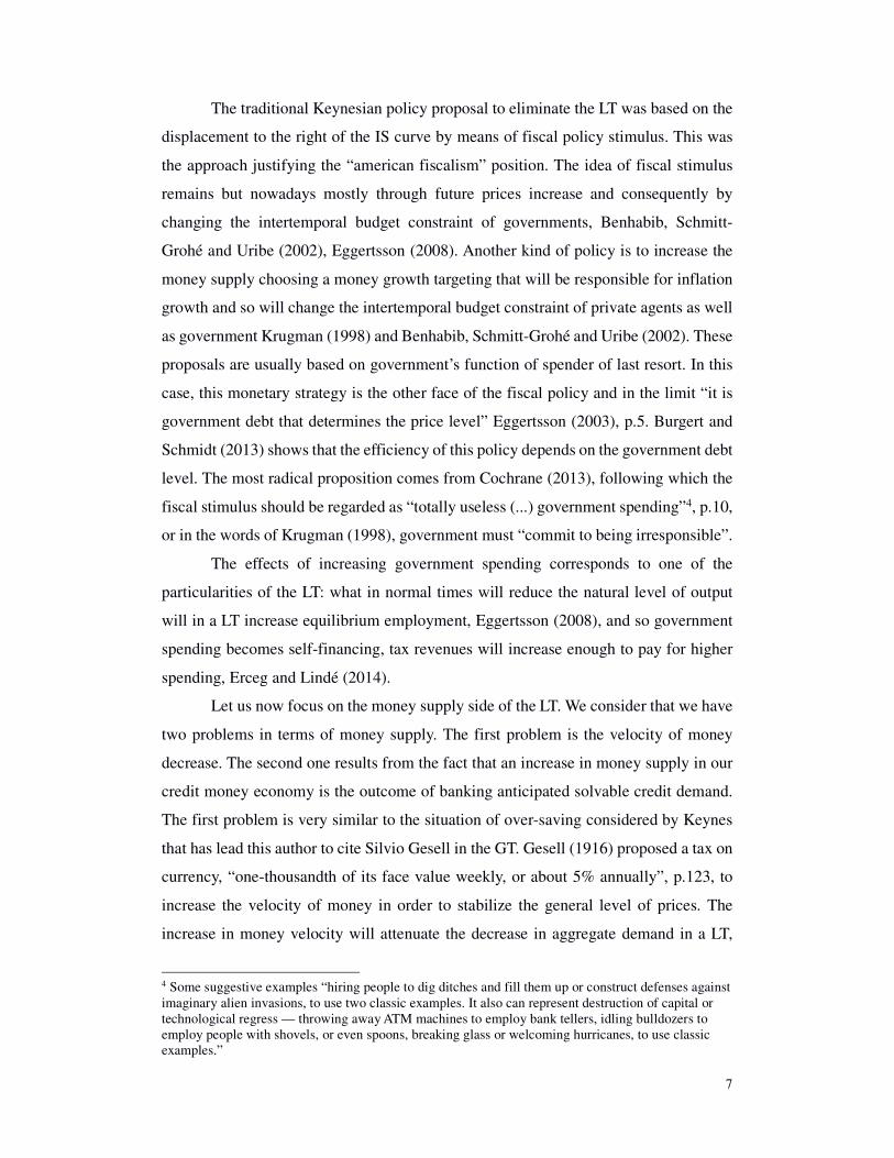
Figure 10. Inverse of the VAR roots on the unit circle (VECM – 1st sub-period)

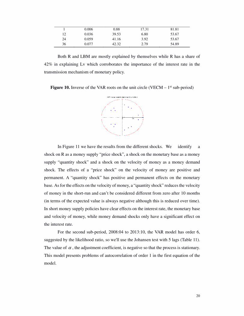
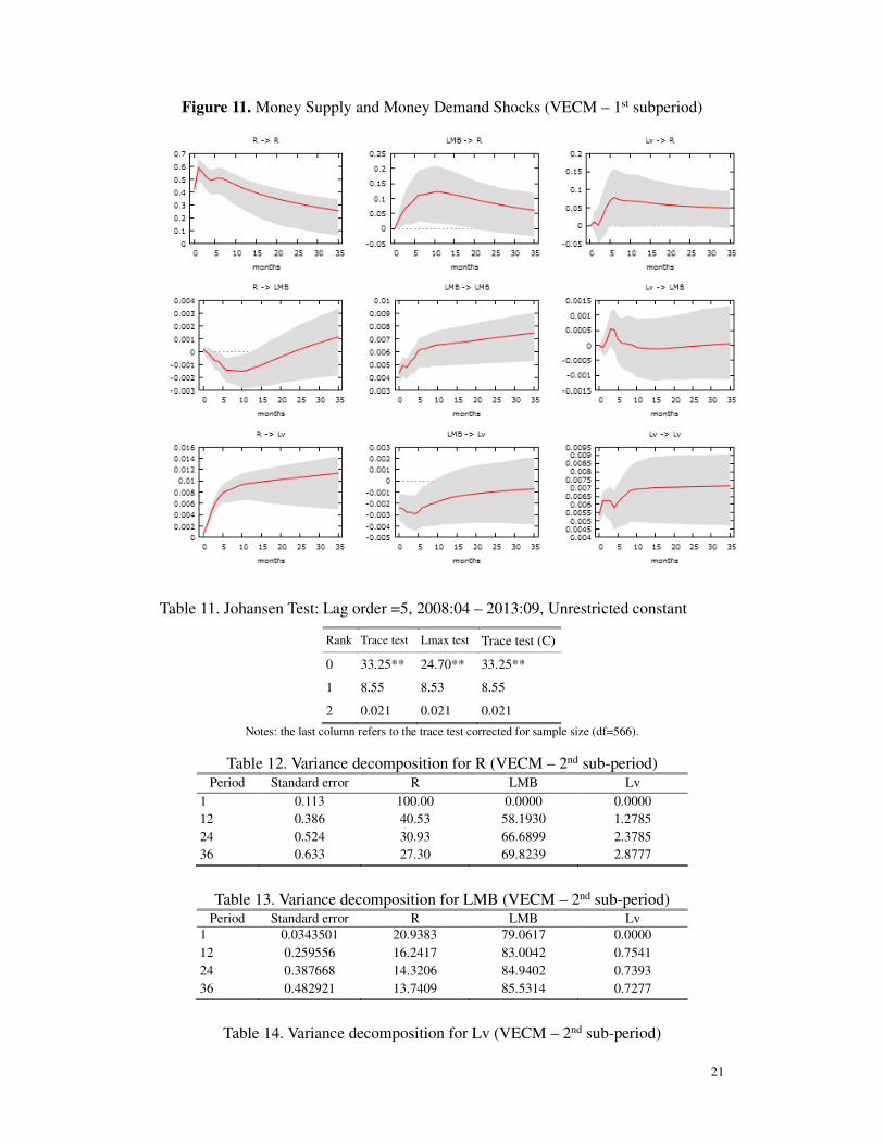
In Figure 11 we have the results from the different shocks. We identify a

shock on R as a money supply “price shock”, a shock on the monetary base as a money

supply “quantity shock” and a shock on the velocity of money as a money demand

shock. The effects of a “price shock” on the velocity of money are positive and

permanent. A “quantity shock” has positive and permanent effects on the monetary

base. As for the effects on the velocity of money, a “quantity shock” reduces the velocity

of money in the short-run and can’t be considered different from zero after 10 months

(in terms of the expected value is always negative although this is reduced over time).

In short money supply policies have clear effects on the interest rate, the monetary base

and velocity of money, while money demand shocks only have a significant effect on

the interest rate.

For the second sub-period, 2008:04 to 2013:10, the VAR model has order 6,

suggested by the likelihood ratio, so we'll use the Johansen test with 5 lags (Table 11).

The value of α , the adjustment coefficient, is negative so that the process is stationary.

This model presents problems of autocorrelation of order 1 in the first equation of the

model.

21

Figure 11. Money Supply and Money Demand Shocks (VECM – 1st subperiod)

Table 11. Johansen Test: Lag order =5, 2008:04 – 2013:09, Unrestricted constant

Rank Trace test Lmax test Trace test (C)

0 33.25** 24.70** 33.25**

1 8.55 8.53 8.55

2 0.021 0.021 0.021

Notes: the last column refers to the trace test corrected for sample size (df=566).

Table 12. Variance decomposition for R (VECM – 2nd sub-period)

Period Standard error R LMB Lv

1 0.113 100.00 0.0000 0.0000

12 0.386 40.53 58.1930 1.2785

24 0.524 30.93 66.6899 2.3785

36 0.633 27.30 69.8239 2.8777

Table 13. Variance decomposition for LMB (VECM – 2nd sub-period)

Period Standard error R LMB Lv

1 0.0343501 20.9383 79.0617 0.0000

12 0.259556 16.2417 83.0042 0.7541

24 0.387668 14.3206 84.9402 0.7393

36 0.482921 13.7409 85.5314 0.7277

Table 14. Variance decomposition for Lv (VECM – 2nd sub-period)

22

Period Standard error R LMB Lv

1 0.0129823 12.0495 3.8009 84.1496

12 0.074697 2.1950 47.2433 50.5617

24 0.107678 1.1501 49.7129 49.1370

36 0.132694 0.8167 50.5285 48.6548

Tables 12, 13, and 14 contain the variance decomposition of the variables in the

VECM. The fact that LMB and Lv have shares of 70% and 2.9%, respectively, in the

explanation of R is understood due to the period under analysis. QE policy is a

combination: of an increase in monetary base and a decrease in the interest rate; and

relatively lower velocity of money has a reduced impact on the evolution of interest

rates. The money velocity has also a reduced impact on the evolution of the monetary

base (Table 13). The variance of this last variable is explained by the interest rate (14%)

and by itself (85%). The variance of the velocity of money is explained in practically

equal parts by itself and by the monetary base (Table 14). It is also important to

highlight the fact that R lose explanatory power on Lv and this fact maybe an indicator

of a possible ineffectiveness of the MP in the crisis period.

In Figure 12 we see that this model is stable: the associated roots lie inside the

unit circle.

Figure 12. Inverse of the VAR roots on the unit circle (VECM – 2nd sub-period)

Like in the previous sub-period analysis it appears (Figure 13) that a “price

shock” has a positive effect on Lv (though not different from zero after 4 months). A

“quantity shock” has a negative effect on R during 3 months. A “quantity shock” has

also a permanent and positive effect on the variable itself and a negative effect on Lv

(tough after about 2 months this effect is not different from zero). In short, in terms of

monetary policy a “price shock” or a “quantity shock” are ineffective since they have

no significant impact on LMB and Lv. Finally money demand shocks does not

significantly affect R or LMB but they have a very high degree of inertia in itself.

23

Figure 13. Money Supply and Money Demand Shocks (Model B – 2nd sub-period)

Thus, as we have already confirmed with the VAR model, we confirm that

monetary policy does not exert significant effects on non-banking economy in the

second period analyzed, unlike what happened in the first. This second period is likely

to be identified as a period of LT.

4. Concluding Remarks

With this paper we study the phenomenon of LT. We started with the definition

of LT from the origins of the concept in the Keynesian literature to the more recent

definitions. We also discuss the consequences of the usual definition and some of the

episodes. The understanding of the LT allows the monetary authorities to get out its

vicious circle. Contrary to the common vision that bases the phenomenon on the

demand for money we propose to see it as a money supply rupture.

To test our thesis about LT we have looked at the newly QE policy adopted by

the FED and its effects on the U.S. economy. We have divided the period of study

(1959:01 to 2013:10) in a “normal period” (1959:01 to 2008:03) and a “crisis period”

(2008:04 to 2013:12). This last period is identified as having the characteristics of a LT

24

episode. We demonstrate that the decrease of the income velocity of money is important

but far from the almost-zero value predicted by the traditional and current definition.

The most important element of a LT is not the evolution of the income velocity of

money but the evolution of the money multiplier.

We propose a VAR model to analyze the evolution of the monetary base and the

money supply. For the first period we prove the exogeneity of the money supply and

the null effect of the demand for money over the monetary base. In the second period a

shock on the money supply quickly cancels its effects on M1 and money demand shocks

affects permanently the monetary base. The relevant conclusion with this model is the

ineffectiveness of money supply shocks in the current situation since 2008:04 to the

present.

We have also studied a monetary equilibrium model with short and long term

relations between the interest rate (Federal Funds Rate), the monetary base and the

income velocity of money. These variables are cointegrated of order 1 and so we use a

VECM model to simulate shocks in the two selected sub-periods. During the normal

period the effects of a monetary “price shock” is positive and permanent on the income

velocity of money and a “quantitative shock” has permanent effects on the monetary

base. Resuming our results money supply policies have clear effects on the interest rate,

the monetary base and the income velocity of money and money demand shocks have

only significant effects on the interest rate. The same type of model for the period after

2008:4 gives very different results. A monetary policy “price shock” or a “quantity

shock” are ineffective since they have no significant impact on the monetary base and

in the income velocity of money. Money demand shocks do not significantly affect the

interest rate or the monetary base. Instead they exhibit a high level of inertia on

themselves.

Our thesis about LT takes the banking sector as the central problem that might

explain it. Banks can create money but they simple do not do it because they consider

that there is no acceptable level of risk from bank credit demand. The creation of

inflation expectations as a way to originate incentives for banking borrowing has to be

compatible with money supply targets and these should be realistic with banking

lending. There is another way to increase inflation expectations, through government

expenditures, but this latter is not available. It is well-known that almost everywhere

government as a spender of last resort is limited by high levels of indebtedness.

25

References

Auerbach, A. and M. Obstfeld (2004), "The Case for Open-Market Purchases in a Liquidity Trap".

American Economic Review, 95:1, pp. 110-37.

Benhabib, J., S. Schmitt-Grohé and M. Uribe (2002), "Avoiding Liquidity Traps". Journal of Political

Economy, 110:3, pp. 535-63.

Bernanke, B. 2000, "Japanese Monetary Policy: A Case of Self-Induced Paralysis?", in A. S. Posen and

R. Mikitani eds., Japan’s Financial Crisis and Its Parallels to U.S. Experience. Washington, D.C.:

Institute for International Economics.

-------- (2002), "Deflation: Making Sure ‘It’ Doesn’t Happen Here". Speech, Federal Reserve Board,

November:21th.

Blinder, A. (2000), "Monetary Policy at the Zero Lower Bound: Balancing the Risks". Journal of Money,

Credit, and Banking, 32:4, pp. 1093-99.

Bofinger, P. (2001), Monetary Policy. Goals, Institutions, Strategies, and Instruments. Oxford: Oxford

University Press.

Boianovsky, M. (2003), "The IS-LM Model and the Liquidity Trap Concept: From Hicks to Krugman".

Proceedings of the 31th Brazilian Economics Meeting.

Bordo, M. and A. Schwartz (2003), "IS-LM and Monetarism". NBER W. P., 9713.

Brunner, K. and A. H. Meltzer (1968), "Liquidity Traps for Money, Bank Credit, and Interest Rates".

Journal of Political Economy, 76:1.

Buiter, W. H. and N. Panigirtzoglou (1999), "Liquidity Traps: how to avoid them and how to escape

them". NBER W. P., 7245.

Burgert, M. and S. Schmidt (2013), "Dealing with a Liquidity Trap when Government Debt Matters:

optimal time-consistent monetary and fiscal policy". ECB, W. P., 1622.

Cochrane, J. H. (2013), "The New-Keynesian Liquidity Trap". NBER, W.P., 19476.

Dale, S. and A. Haldane (1993), "A simple Model of Money, Credit and Aggregate Demand". Bnak of

England W.P., 7.

Dasgupta, S. (2009), "Comment on Luigi Zingales: Why Not Consider Maximum Reserve Ratios?". The

Economists’ Voice, 6:4.

Edlin, A. S. and D. M. Jaffee (2009), "Show Me the Money". The Economists’ Voice electronic journal,

6:4.

Eggertsson, G. (2005), "Great Expectations and the End of the Depression.". Federal Reserve Bank of

New York, Staff Report, 234.

-------- 2008, "Liquidity Trap", in S. D. a. L. Blume ed., The New Palgrave Dictionary of Economics.

http://www.dictionaryofeconomics.com/article?id=pde2008_L000237: Macmillan.

Eggertsson, G. and P. Krugman (2012), "Debt, Deleveraging, and the Liquidity Trap: A Fisher-Minsky-

Koo Approach". Quarterly Journal of Economics, 127:3, pp. 1469-513.

Eggertsson, G. and M. Woodford (2003), "The Zero Bound on Interest Rates and Optimal Monetary

Policy". Brookings Papers on Economic Activity, 1, pp. 212-19.

Eggertsson, G. B. (2003), "How to Fight Deflation in a Liquidity Trap: Committing to Being

Irresponsible". IMF Working Paper, 03/64.

Erceg, C. and J. Lindé (2014), "Is There a Fiscal Free Lunch in a Liquidity Trap?". Journal of the

European Economic Association, 12:1, pp. 73-107.

Fawley, B. W. and C. J. Neely (2013), "Four Stories of Quantitative Easing". Federal Reserve Bank of

St. Louis Review, 95:1, pp. 51-88.

Fisher, I. (1933), "The Debt-Deflation Theory of Great Depressions". Econometrica, 1:4.

Friedman, M. 1956, "The Quantity Theory of Money - A Restatement", in M. Friedman ed., Studies in

the Quantity Theory of Money. Chicago: University of Chicago Press, pp. 3-21.

Gesell, S. (1916), The Natural Economic Order, translated by Philip Pye M.A.

http://www.pdfarchive.info/pdf/G/Ge/Gesell\_Silvio\_-\_The\_Natural\_Economic\_Order.pdf.

Guerrieri, V. and G. Lorenzoni (2011), "Credit Crises, Precautionary Savings, and the Liquidity Trap".

NBER Working Paper, 17583.

Haberler, G. (1937), Prosperity and Depression. Geneve: League of Nations.

Hall, R. E. (2011), "The Long Slump". American Economic Review, 101:2, pp. 431-69.

Hanes, C. (2006), "The Liquidity Trap and U.S. Interest Rates in the 1930s". Journal of Money, Credit

and Banking, 38:1, pp. 163-94.

Hansen, A. H. (1953), A Guide to Keynes. New York: McGraw-Hill,.

Hicks, J. R. (1937), "Mr. Keynes and the Classics: A Suggested Interpretation". Econometrica, 5:2, pp.

147-59.

26

Hoffman, D. and R. Rasche. (1996), Aggregate Money Demand Functions. Boston: Kluwer Academic

Publishers.

Humphrey, T. (1974), "The Quantity Theory of Money: Its Historical Evolution and Role in Policy

Debates". Economic Review, Federal Reserve Bank of Richmond:May/June, pp. 1-18.

-------- (2004), "Classical Deflation Theory". Economic Quarterly, Federal Reserve Bank of Richmond,

90/1:Winter, pp. 11-32.

Kaldor, N. (1939), "Speculation and Economic Stability". Review of Economic Studies, 7:1, pp. 1-27.

Keynes, J. M. (1936), The General Theory of Employment, Interest and Money. London: The CW of

JMK, Volume VII, Royal Economic Society, 1973.

--------. (1973), The General Theory and After, Part II, Defense and Development. London: Royal

Economic Society.

Koo, R., , Wiley. (2009), The Holy Grail of Macroeconomics: Lessons from Japan’s Great Recession.

Singapore: John Wiley & Sons; Revised Edition

Korinek, A. and A. Simsek (2013), "Liquidity Trap and Excessive Leverage". Koç University-TUSIAD

Economic Research Forum WP, 1410.

Krugman, P. (1998), "It’s Baaack: Japan’s Slump and the Return of the Liquidity Trap". Brookings Papers

on Economic Activity, 2, pp. 137-205.

Mian, A. and A. Sufi (2010), "Household Leverage and the Recession of 2007-09". IMF Economic

Review, 58:1, pp. 74-117.

Modigliani, F. (1944), "Liquidity Preference and the Teory of Interest and Money". Econometrica, 12:1,

pp. 45-88.

Orphanides, A. and V. Wieland (2000), "Efficient Monetary Policy Design near Price Stability". Journal

of the Japanese and International Economies, 14, pp. 327-65.

Patinkin, D. (1974), "The Role of the «Liquidity Trap» in Keynesian Economics". Banca Nazionale Del

Lavoro Q R, 26:108, pp. 3-11.

Pigou, A. C. (1943), "The Classical Steady State". Economic Journal, 53:2, pp. 343-51.

Pollin, R. (2012), "The Great U.S: Liquidity Trap of 2009-11: Are We Stuck Pushing on Strings?". Policy

Economic Research Institute, University of Masachusetts, W.P., 284.

Rhodes, J. R. (2011), "The Curious Case of the Liquidity Trap". The Hikone Ronso, 387, pp. 8-21.

Robertson, D. H. (1940), Essays in Monetary Economics. London: P.S. King.

Robinson, J. (1951), "The Rate of Interest". Econometrica, 19:2, pp. 92-111.

Sax, C. and P. Steiner (2013), "Methods for Temporal Disaggregation and Interpolation of Time Series".

The R Journal, 5:2, pp. 80-87.

Shirakawa, M. (2002), "One Year under ‘Quantitative Easing’". Institute of Monetary and Economic

Studies, Bank of Japan, Discussion Paper no. 2002-E-3.

Sumner, S. (2002), "Some Observations on the Return of the Liquidity Trap". Cato Journal, 21:3, pp.

481-90.

Sutch, R. (2009), "The Liquidity Trap: A Lesson from Macroeconomic History for Today". The Center

for Social and Economic Policy, University of California, Riverside, W.P.

Svensson, L. 1999, "How Should Monetary Policy be Conducted in an Era of Price Stability?", in

FRBKC ed., In New Challenges for Monetary Policy. Proceedings - Economic Policy Symposium -

Jackson Hole: Federal Reserve Bank of Kansas City, pp. 195-259.

-------- (2001), "The Zero Bound in an Open Economy: A Foolproof Way of Escaping from a Liquidity

Trap". Institute for Monetary and Economic Studies, Bank of Japan, 19:S1, pp. 277-312.

-------- 2002, "Monetary Policy and Real Stabilization", in FRBKC ed., Rethinking Stabilization Policy,

A Symposium Sponsored by the Federal Reserve Bank of Kansas City. Proceedings - Economic Policy

Symposium - Jackson Hole: Federal Reserve Bank of Kansas City, pp. 261-312.

-------- (2003), " Escaping from a Liquidity Trap and Deflation: The Foolproof Way and Others". Journal

of Economic Perspectives, 17:4, pp. 145-66.

-------- (2006), "Monetary Policy and Japan’s Liquidity Trap". CEPS W.P., 126.

Tobin, J. (1947), "Liquidity Preference and Monetary Policy". Review of Economics and Statistics, 29:2,

pp. 124-31.

ESTUDOS DO G.E.M.F. (Available on-line at http://www.uc.pt/feuc/gemf )

2015-06 A Monetary Analysis of the Liquidity Trap - João Braz Pinto & João Sousa Andrade

2015-05 Efficient Skewness/Semivariance Portfolios - Rui Pedro Brito, Hélder Sebastião & Pedro Godinho

2015-04 Size Distribution of Portuguese Firms between 2006 and 2012 - Rui Pascoal, Mário Augusto & Ana M. Monteiro

2015-03 Optimum Currency Areas, Real and Nominal Convergence in the European Union - João Sousa Andrade & António Portugal Duarte

2015-02 Estimating State-Dependent Volatility of Investment Projects: A Simulation Approach - Pedro Godinho

2015-01 Is There a Trade-off between Exchange Rate and Interest Rate Volatility? Evidence from an M-GARCH Model - António Portugal Duarte, João Sousa Andrade & Adelaide Duarte

2014-25 Portfolio Choice Under Parameter Uncertainty: Bayesian Analysis and Robust Optimization

Comparison - António A. F. Santos, Ana M. Monteiro & Rui Pascoal

2014-24 Crowding-in and Crowding-out Effects of Public Investments in the Portuguese Economy - João Sousa Andrade & António Portugal Duarte

2014-23 Are There Political Cycles Hidden Inside Government Expenditures? - Vítor Castro & Rodrigo Martins

2014-22 The Nature of Entrepreneurship and its Determinants: Opportunity or Necessity? - Gonçalo Brás & Elias Soukiazis

2014-21 Estado Social, Quantis, Não-Linearidades e Desempenho Económico: Uma Avaliação Empírica - Adelaide Duarte, Marta Simões & João Sousa Andrade

2014-20 Assessing the Impact of the Welfare State on Economic Growth: A Survey of Recent Developments - Marta Simões, Adelaide Duarte & João Sousa Andrade

2014-19 Business Cycle Synchronization and Volatility Shifts - Pedro André Cerqueira

2014-18 The Public Finance and the Economic Growth in the First Portuguese Republic - Nuno Ferraz Martins & António Portugal Duarte

2014-17 On the Robustness of Minimum Wage Effects: Geographically-Disparate Trends and Job Growth Equations - John T. Addison, McKinley L. Blackburn & Chad D. Cotti

2014-16 Determinants of Subjective Well-Being in Portugal: A Micro-Data Study - Sara Ramos & Elias Soukiazis

2014-15 Changes in Bargaining Status and Intra-Plant Wage Dispersion in Germany. A Case of (Almost) Plus Ça Change? - John T. Addison, Arnd Kölling & Paulino Teixeira

2014-14 The Renewables Influence on Market Splitting: the Iberian Spot Electricity Market - Nuno Carvalho Figueiredo, Patrícia Pereira da Silva & Pedro Cerqueira

2014-13 Drivers for Household Electricity Prices in the EU: A System-GMM Panel Data Approach - Patrícia Pereira da Silva & Pedro Cerqueira

2014-12 Effectiveness of Intellectual Property Regimes: 2006-2011 - Noemí Pulido Pavón & Luis Palma Martos

2014-11 Dealing with Technological Risk in a Regulatory Context: The Case of Smart Grids - Paulo Moisés Costa, Nuno Bento & Vítor Marques

2014-10 Stochastic Volatility Estimation with GPU Computing - António Alberto Santos & João Andrade

Estudos do GEMF

2014-09 The Impact of Expectations, Match Importance and Results in the Stock Prices of European Football Teams - Pedro Godinho & Pedro Cerqueira

2014-08 Is the Slovak Economy Doing Well? A Twin Deficit Growth Approach - Elias Soukiazis, Eva Muchova & Pedro A. Cerqueira

2014-07 The Role of Gender in Promotion and Pay over a Career - John T. Addison, Orgul D. Ozturk & Si Wang

2014-06 Output-gaps in the PIIGS Economies: An Ingredient of a Greek Tragedy - João Sousa Andrade & António Portugal Duarte

2014-05 Software Piracy: A Critical Survey of the Theoretical and Empirical Literature - Nicolas Dias Gomes, Pedro André Cerqueira & Luís Alçada Almeida

2014-04 Agriculture in Portugal: Linkages with Industry and Services - João Gaspar, Gilson Pina & Marta C. N. Simões

2014-03 Effects of Taxation on Software Piracy Across the European Union - Nicolas Dias Gomes, Pedro André Cerqueira & Luís Alçada Almeida

2014-02 A Crise Portuguesa é Anterior à Crise Internacional - João Sousa Andrade

2014-01 Collective Bargaining and Innovation in Germany: Cooperative Industrial Relations? - John T. Addison, Paulino Teixeira, Katalin Evers & Lutz Bellmann

2013-27 Market Efficiency, Roughness and Long Memory in the PSI20 Index Returns: Wavelet and

Entropy Analysis - Rui Pascoal & Ana Margarida Monteiro

2013-26 Do Size, Age and Dividend Policy Provide Useful Measures of Financing Constraints? New Evidence from a Panel of Portuguese Firms - Carlos Carreira & Filipe Silva

2013-25 A Política Orçamental em Portugal entre Duas Intervenções do FMI: 1986-2010 - Carlos Fonseca Marinheiro

2013-24 Distortions in the Neoclassical Growth Model: A Cross-Country Analysis - Pedro Brinca

2013-23 Learning, Exporting and Firm Productivity: Evidence from Portuguese Manufacturing and Services Firms - Carlos Carreira

2013-22 Equity Premia Predictability in the EuroZone - Nuno Silva

2013-21 Human Capital and Growth in a Services Economy: the Case of Portugal - Marta Simões & Adelaide Duarte

2013-20 Does Voter Turnout Affect the Votes for the Incumbent Government? - Rodrigo Martins & Francisco José Veiga

2013-19 Determinants of Worldwide Software Piracy Losses - Nicolas Dias Gomes, Pedro André Cerqueira & Luís Alçada Almeida

2013-18 Despesa Pública em Educação e Saúde e Crescimento Económico: Um Contributo para o Debate sobre as Funções Sociais do Estado - João Sousa Andrade, Marta Simões & Adelaide P. S. Duarte

2013-17 Duration dependence and change-points in the likelihood of credit booms ending - Vitor Castro & Megumi Kubota

2013-16 Job Promotion in Mid-Career: Gender, Recession and ‘Crowding’ - John T. Addison, Orgul D. Ozturk & Si Wang

2013-15 Mathematical Modeling of Consumer's Preferences Using Partial Differential Equations - Jorge Marques

2013-14 The Effects of Internal and External Imbalances on Italy´s Economic Growth. A Balance of Payments Approach with Relative Prices No Neutral. - Elias Soukiazis, Pedro André Cerqueira & Micaela Antunes

Estudos do GEMF

2013-13 A Regional Perspective on Inequality and Growth in Portugal Using Panel Cointegration Analysis - Marta Simões, João Sousa Andrade & Adelaide Duarte

2013-12 Macroeconomic Determinants of the Credit Risk in the Banking System: The Case of the GIPSI - Vítor Castro

2013-11 Majority Vote on Educational Standards - Robert Schwager

2013-10 Productivity Growth and Convergence: Portugal in the EU 1986-2009 - Adelaide Duarte, Marta Simões & João Sousa Andrade

2013-09 What Determines the Duration of a Fiscal Consolidation Program? - Luca Agnello, Vítor Castro & Ricardo M. Sousa

2013-08 Minimum Wage Increases in a Recessionary Environment - John T. Addison, McKinley L. Blackburn & Chad D. Cotti

2013-07 The International Monetary System in Flux: Overview and Prospects - Pedro Bação, António Portugal Duarte & Mariana Simões

2013-06 Are There Change-Points in the Likelihood of a Fiscal Consolidation Ending? - Luca Agnello, Vitor Castro & Ricardo M. Sousa

2013-05 The Dutch Disease in the Portuguese Economy - João Sousa Andrade & António Portugal Duarte

2013-04 Is There Duration Dependence in Portuguese Local Governments’ Tenure? - Vítor Castro & Rodrigo Martins

2013-03 Testing for Nonlinear Adjustment in the Portuguese Target Zone: Is there a Honeymoon Effect? - António Portugal Duarte, João Soares da Fonseca & Adelaide Duarte

2013-02 Portugal Before and After the European Union - Fernando Alexandre & Pedro Bação

2013-01 The International Integration of the Eastern Europe and two Middle East Stock Markets - José Soares da Fonseca

2012-21 Are Small Firms More Dependent on the Local Environment than Larger Firms? Evidence

from Portuguese Manufacturing Firms - Carlos Carreira & Luís Lopes

2012-20 Macroeconomic Factors of Household Default. Is There Myopic Behaviour? - Rui Pascoal

2012-19 Can German Unions Still Cut It? - John Addison, Paulino Teixeira, Jens Stephani & Lutz Bellmann

2012-18 Financial Constraints: Do They Matter to R&D Subsidy Attribution? - Filipe Silva & Carlos Carreira

2012-17 Worker Productivity and Wages: Evidence from Linked Employer-Employee Data - Ana Sofia Lopes & Paulino Teixeira

2012-16 Slovak Economic Growth and the Consistency of the Balance-of-Payments Constraint Approach - Elias Soukiazis & Eva Muchova

2012-15 The Importance of a Good Indicator for Global Excess Demand - João Sousa Andrade & António Portugal Duarte

2012-14 Measuring Firms' Financial Constraints: A Rough Guide - Filipe Silva & Carlos Carreira

2012-13 Convergence and Growth: Portugal in the EU 1986-2010 - Marta Simões, João Sousa Andrade & Adelaide Duarte

2012-12 Where Are the Fragilities? The Relationship Between Firms’ Financial Constraints, Size and Age - Carlos Carreira & Filipe Silva

2012-11 An European Distribution of Income Perspective on Portugal-EU Convergence - João Sousa Andrade, Adelaide Duarte & Marta Simões

Estudos do GEMF

2012-10 Financial Crisis and Domino Effect - Pedro Bação, João Maia Domingues & António Portugal Duarte

2012-09 Non-market Recreational Value of a National Forest: Survey Design and Results - Paula Simões, Luís Cruz & Eduardo Barata

2012-08 Growth rates constrained by internal and external imbalances and the role of relative prices: Empirical evidence from Portugal - Elias Soukiazis, Pedro André Cerqueira & Micaela Antunes

2012-07 Is the Erosion Thesis Overblown? Evidence from the Orientation of Uncovered Employers - John Addison, Paulino Teixeira, Katalin Evers & Lutz Bellmann

2012-06 Explaining the interrelations between health, education and standards of living in Portugal. A simultaneous equation approach - Ana Poças & Elias Soukiazis

2012-05 Turnout and the Modeling of Economic Conditions: Evidence from Portuguese Elections - Rodrigo Martins & Francisco José Veiga

2012-04 The Relative Contemporaneous Information Response. A New Cointegration-Based Measure of Price Discovery - Helder Sebastião

2012-03 Causes of the Decline of Economic Growth in Italy and the Responsibility of EURO. A Balance-of-Payments Approach. - Elias Soukiazis, Pedro Cerqueira & Micaela Antunes

2012-02 As Ações Portuguesas Seguem um Random Walk? Implicações para a Eficiência de Mercado e para a Definição de Estratégias de Transação - Ana Rita Gonzaga & Helder Sebastião

2012-01 Consuming durable goods when stock markets jump: a strategic asset allocation approach - João Amaro de Matos & Nuno Silva

2011-21 The Portuguese Public Finances and the Spanish Horse

- João Sousa Andrade & António Portugal Duarte 2011-20 Fitting Broadband Diffusion by Cable Modem in Portugal

- Rui Pascoal & Jorge Marques 2011-19 A Poupança em Portugal

- Fernando Alexandre, Luís Aguiar-Conraria, Pedro Bação & Miguel Portela 2011-18 How Does Fiscal Policy React to Wealth Composition and Asset Prices?

- Luca Agnello, Vitor Castro & Ricardo M. Sousa 2011-17 The Portuguese Stock Market Cycle: Chronology and Duration Dependence

-Vitor Castro 2011-16 The Fundamentals of the Portuguese Crisis

- João Sousa Andrade & Adelaide Duarte 2011-15 The Structure of Collective Bargaining and Worker Representation: Change and Persistence

in the German Model - John T. Addison, Paulino Teixeira, Alex Bryson & André Pahnke

2011-14 Are health factors important for regional growth and convergence? An empirical analysis for the Portuguese districts - Ana Poças & Elias Soukiazis

2011-13 Financial constraints and exports: An analysis of Portuguese firms during the European monetary integration - Filipe Silva & Carlos Carreira

2011-12 Growth Rates Constrained by Internal and External Imbalances: a Demand Orientated Approach - Elias Soukiazis, Pedro Cerqueira & Micaela Antunes

2011-11 Inequality and Growth in Portugal: a time series analysis - João Sousa Andrade, Adelaide Duarte & Marta Simões

2011-10 Do financial Constraints Threat the Innovation Process? Evidence from Portuguese Firms - Filipe Silva & Carlos Carreira

Estudos do GEMF

2011-09 The State of Collective Bargaining and Worker Representation in Germany: The Erosion Continues - John T. Addison, Alex Bryson, Paulino Teixeira, André Pahnke & Lutz Bellmann

2011-08 From Goal Orientations to Employee Creativity and Performance: Evidence from Frontline Service Employees - Filipe Coelho & Carlos Sousa

2011-07 The Portuguese Business Cycle: Chronology and Duration Dependence - Vitor Castro

2011-06 Growth Performance in Portugal Since the 1960’s: A Simultaneous Equation Approach with Cumulative Causation Characteristics - Elias Soukiazis & Micaela Antunes

2011-05 Heteroskedasticity Testing Through Comparison of Wald-Type Statistics - José Murteira, Esmeralda Ramalho & Joaquim Ramalho

2011-04 Accession to the European Union, Interest Rates and Indebtedness: Greece and Portugal - Pedro Bação & António Portugal Duarte

2011-03 Economic Voting in Portuguese Municipal Elections - Rodrigo Martins & Francisco José Veiga

2011-02 Application of a structural model to a wholesale electricity market: The Spanish market from January 1999 to June 2007 - Vítor Marques, Adelino Fortunato & Isabel Soares

2011-01 A Smoothed-Distribution Form of Nadaraya-Watson Estimation - Ralph W. Bailey & John T. Addison

A série Estudos do GEMF foi iniciada em 1996.