Estudos e Documentos de Trabalho

Working Papers

15 | 2006

COMPUTING GENERAL EQUILIBRIUM MODELS WITH OCCUPATIONAL

CHOICE AND FINANCIAL FRICTIONS

António AntunesTiago Cavalcanti

Anne Villamil

September 2006

The analyses, opinions and findings of these papers represent the views of the

authors, they are not necessarily those of the Banco de Portugal.

Please address correspondence to

António Antunes

Economic Research Department

Banco de Portugal, Av. Almirante Reis no. 71, 1150-012 Lisboa, Portugal;

Tel.: 351 21 312 8246, Email: aantunes@bportugal.pt

Computing General Equilibrium Models

with Occupational Choice and Financial Frictions∗

Antonio Antunes† Tiago Cavalcanti‡ Anne Villamil§

September 29, 2006

Abstract

This paper establishes the existence of a stationary equilibrium and a procedure to compute

solutions to a class of dynamic general equilibrium models with two important features. First, oc-

cupational choice is determined endogenously as a function of heterogeneous agent type, which is

defined by an agent’s managerial ability and capital bequest. Heterogeneous ability is exogenous

and independent across generations. In contrast, bequests link generations and the distribution of

bequests evolves endogenously. Second, there is a financial market for capital loans with a deadweight

intermediation cost and a repayment incentive constraint. The incentive constraint induces a non-

convexity. The paper proves that the competitive equilibrium can be characterized by the bequest

distribution and factor prices, and uses the monotone mixing condition to ensure that the stationary

bequest distribution that arises from the agent’s optimal behavior across generations exists and is

unique. The paper next constructs a direct, non-parametric approach to compute the stationary

solution. The method reduces the domain of the policy function, thus reducing the computational

complexity of the problem.

JEL Classification: C62; C63; E60; G38.

Keywords: Existence; Computation; Dynamic general equilibrium; Non-convexity.

1 Introduction

This paper establishes the existence of a stationary equilibrium and a procedure to compute solutionsto dynamic general equilibrium models with occupational choice and financial frictions. Occupationalchoice models are common in macroeconomics and there is a voluminous literature on financial marketfrictions.1 These models often have non-convexities which give rise to discontinuous stochastic behavior(e.g., Antunes, Cavalcanti and Villamil, 2006); standard fixed point existence arguments that require

∗We thank Antonio Sa Barreto, Evangelos Benos, Gabriele Camera, Nicholas Yannelis and a referee for helpful sug-gestions. We have also benefited from comments by audiences at the SED Annual Meeting 2005, EEA Congress 2005,SAET Annual Meeting 2005, Minneapolis Fed, University of Illinois, Purdue University, the University of Kentucky andthe University of Singapore. This material is based upon work supported by the National Science Foundation under grantSES-031839. Cavalcanti is also thankful to Conselho Nacional de Desenvolvimento Cientıfico e Tecnologico (CNPq, Brazil)for financial support. We are responsible for any remaining errors.

†Banco de Portugal, Departamento de Estudos Economicos, and Faculdade de Economia, Universidade Nova de Lisboa.Email: ara@fe.unl.pt.

‡Departamento de Economia, Universidade Federal de Pernambuco, INOVA, Faculdade de Economia, Universidade Novade Lisboa. Email: cavalcan@fe.unl.pt.

§Corresponding author: Anne P. Villamil, Department of Economics, University of Illinois at Urbana-Champaign. Email:avillami@uiuc.edu.

1Examples of occupational choice models are Banerjee and Newman (1993), Erosa (2001), Lloyd-Ellis and Bernhardt(2000) and Antunes and Cavalcanti (2005). Examples of models with financial frictions are Antinolfi and Huybens (1998),Betts and Bhattacharya (1998) and Boyd and Smith (1998).

1

continuity are not applicable.2 Hopenhayn and Prescott (1992) remedy this problem by proving existenceof stationary equilibria for stochastically monotone processes. They use the Knaster-Tarski fixed pointtheorem to prove existence of fixed point mappings on compact sets of measures that are increasingwith respect to a stochastic ordering (monotone). Our contribution is two-fold. First, we show how theHopenhayn and Prescott result can be applied to this class of dynamic general equilibrium models toprove existence of a stationary equilibrium. Second, we construct a direct, non-parametric approach tocompute the stationary solution. Our method reduces the domain of the policy function, thus reducingthe computational complexity of the problem.

The class of models that we consider have two important features. First, occupational choice is deter-mined endogenously as a function of heterogeneous agent type. Agents are endowed with different innateabilities to manage a firm (cf., Lucas, 1978) and different bequests (cf., Antunes et al., 2006). Heteroge-neous ability is exogenous, in the sense that managerial ability is drawn from a fixed distribution, andis independent within and across generations. In contrast, agents choose consumption and bequests tomaximize preferences subject to lifetime wealth. Bequests thus connect generations across time periodsand the distribution of bequests evolves endogenously. Second, there is a financial market for capitalwith two frictions: a deadweight cost to intermediate loans and an incentive constraint to ensure loanrepayment. The incentive constraint induces a non-convexity. We characterize the competitive equilib-rium, and then use a condition derived by Hopenhayn and Prescott, monotone mixing, to ensure thatthe optimal stationary bequest distribution that arises from the stochastic optimization problem existsand is unique.

The paper proceeds as follows. Section 2 contains the model. Section 3 describes optimal consumptionand production behavior. On the production side, agents choose an occupation (to manage a firm orwork) and firm finance (if a manager). Consumers choose consumption and bequests, where bequests linkagents across periods. Section 4 specifies the competitive equilibrium and proves existence of a stationaryequilibrium. We show that there is a unique stationary equilibrium that is fully characterized by a timeinvariant bequest distribution and associated equilibrium factor prices. We use the monotone mixingcondition from Hopenhayn and Prescott (1992) Theorem 2. In our context, this condition characterizestwo types of mobility in the bequest distribution: Given that ability is independent across generations,there is a positive probability that a future descendent of an agent changes occupation (i.e., from workerto entrepreneur or from entrepreneur to worker). Thus the economy experiences occupation mobility, butfrom any initial bequest distribution and any interest rate, convergence to a unique invariant bequestdistribution occurs. Finally, section 5 contains the numerical solution method.

2 The Model

Consider an economy with a continuum of measure one agents who live for one period. Each agentreproduces another such that population is constant. There is one good each period that can be usedfor consumption or production, or left to the next generation as a bequest. Time is discrete and infinite,with t = 0, 1, 2, ....

2Standard Brouwer-Kakutani type fixed point theorems cannot be used because the fixed point mapping is not necessarilycontinuous or upper or lower semi-continuous (cf., Krasa and Yannelis (1994)). The Knaster-Tarski fixed point theorem isnon-topological.

2

2.1 Preferences, Endowments, Technology and Frictions

2.1.1 Preferences

In period t, agent i’s utility is defined over personal consumption and a bequest to offspring, denoted bycit and bi

t+1, respectively. Assume the utility function has the form

U i = u(cit, b

it+1) . (1)

u(·, ·) is twice continuously differentiable, strictly concave and increasing in both arguments. We alsoassume that the utility function satisfies the Inada conditions.3 Preferences are for the bequest and notthe offspring’s utility (cf., Banerjee and Newman, 1993).

2.1.2 Heterogeneous Endowments

Each period, agents are distinguished by their publicly known endowments of initial wealth and ability asentrepreneurs, denoted by (bi

t, xit). The bequest is inherited from the previous generation and generates

a given initial bequest distribution Υ(b). Each individual’s talent for managing, xi, is drawn from a con-tinuous cumulative probability distribution function Γ(x), with x ∈ [x, x], cf., Lucas (1978). Assume thatmanagerial talent is not hereditary. Each individual will choose to be either a worker or an entrepreneur.Entrepreneurs create jobs and manage firm labor n; workers are employed by entrepreneurs at wage wt.For notational convenience, in the remainder of the paper we drop agent superscript i.

2.1.3 Production

Managers operate a technology that uses labor, n, and capital, k, to produce a single consumption good,y, where

y = xf(k, n). (2)

f(·, ·) is twice continuously differentiable, strictly concave and increasing in both arguments. Functionf(·, ·) is also homogenous of degree less than one and satisfies the Inada conditions. Capital fully de-preciates between periods. Managers can operate only one project. The labor and capital markets arecompetitive, with prices w and r, respectively.

2.1.4 Capital Market Frictions, τ and φ

The capital market has two frictions:τ : Agents deposit bequest b in a financial intermediary and earn competitive return r. The interme-

diary lends the resources to entrepreneurs. The part of the loan that is fully collateralized by b costs r;the remainder costs rl = r + τ , where τ is the deadweight cost of intermediation.

φ: Borrowers cannot commit ex-ante to repay, but there is an exogenous enforcement technology. Anagent who defaults on a loan incurs penalty φ, which is the percentage of output forfeited net of wages.This is equivalent to an additive utility punishment, and reflects the strength of contract enforcement:As φ → 1 the penalty is strong; as φ → 0 it is weak.4

3Both Cobb-Douglas and CES utility functions satisfy these restrictions.4As is common in the literature, we choose a proportional punishment for convenience. See Krasa and Villamil (2000)

and Krasa, Sharma and Villamil (2005) for extended analysis of enforcement and debt contracts.

3

3 Optimal Behavior

3.1 Entrepreneurs

Agents who have sufficient resources and managerial ability to become entrepreneurs choose the levelof capital and the number of employees to maximize profit subject to a technological constraint and(possibly) a credit market incentive constraint. Consider first the problem of an entrepreneur for a givenlevel of capital k and wages w:

π(k, x;w) = maxn

xf(k, n)− wn. (3)

This yields the labor demand of each entrepreneur: n(k, x;w). This labor demand is differentiable,continuous in all arguments, increasing in k and x, and decreasing in w. Moreover, limw→0 n(k, x;w) = ∞and limw→∞ n(k, x;w) = 0.

Substituting n(k, x;w) into (3) yields the entrepreneur’s profit function for a given level of capital,π(k, x;w). The profit function is differentiable, continuous in all arguments, increasing in k and x, anddecreasing in w. We now consider two problems: when initial wealth is sufficient to fully finance a firmand when it may not be. Let a be the amount of self-financed capital and l be the amount of fundsborrowed from a financial intermediary.5

Unconstrained Problem. When initial wealth is sufficient for the agent to start her own business withoutresorting to credit finance (i.e., b > a and l = 0), entrepreneurs solve:

Problem 1

maxk≥0

π(k, x;w)− (1 + r)k. (4)

This gives the optimal physical capital level, k∗(x;w, r), which is continuous in all arguments, andstrictly decreasing in factor prices w and r. It can be also shown that limr→−1 k∗(x;w, r) = ∞ andlimr→∞ k∗(x;w, r) = 0. There is no credit market incentive constraint because the firm is entirely self-financed (i.e., no repayment problem exists).

Constrained Problem. When the entrepreneur’s initial wealth may not be sufficient to finance the firm(i.e., b ≥ a and l ≥ 0), the agent will consider loans from the credit market. Since no agent can committo repay a loan, these debt contracts must be self-enforcing.

The entrepreneur now maximizes the net income from operating the project:

Problem 2

V (b, x;w, r) = maxb≥a≥0, l≥0

π(a + l, x;w)− (1 + r)a− (1 + r + τ)l (5)

subject to:

φπ(a + l, x;w) ≥ (1 + r + τ)l. (6)

Feasibility constraint b ≥ a ≥ 0, implicit in the objective, states that the amount of (non-trivial) selffinance, a, cannot exceed the entrepreneur’s bequest, b. Problem 2 yields optimal policy functionsa(b, x;w, r) and l(b, x;w, r) that define the size of each firm,

k(b, x;w, r) = a(b, x;w, r) + l(b, x;w, r).

Restriction (6) is an incentive feasibility constraint which guarantees that ex-ante repayment promiseswill be honored, cf., Kehoe and Levine (1993).6

5Equivalently, a can be interpreted as the part of a loan that is fully collateralized by personal assets and l as theuncollateralized part.

6The restriction requires the percentage of firm profit the financial intermediary seizes in default to be at least as high

4

3.1.1 Solutions to the Entrepreneur’s Problem

The Lagrangian associated with problem 2 is

L =π(a + l, x;w)− (1 + r)a− (1 + r + τ)l

+ λ(φπ(a + l, x;w)− (1 + r + τ)l) + χ(b− a).

The Kuhn-Tucker conditions are:

∂L

∂l= π1(a + l, x;w)− (1 + r + τ) + λ(φπ1(a + l, x;w)− (1 + r + τ)) ≤ 0, (7)

∂L

∂a= π1(a + l, x;w)− (1 + r) + λφπ1(a + l, x;w)− χ ≤ 0, (8)

λ(φπ(a + l, x;w)− (1 + r + τ)l) = 0, (9)

χ(b− a) = 0, (10)

l ≥ 0,∂L

∂ll = 0, a ≥ 0,

∂L

∂aa = 0, λ ≥ 0, χ ≥ 0,

plus the incentive compatibility constraint (6) and constraint b ≥ a. Constrained entrepreneurs are thosefor which l > 0 holds. It is optimal for entrepreneurs to put their entire wealth in their project. Tosee this, assume that constrained entrepreneurs do not put their entire wealth in the project; that is,0 ≤ a < b. Then, from (10), χ = 0, and from (7) at equality and (8) it follows that (1+r)λ+(1+λ)τ ≤ 0,which is a contradiction. Therefore, if entrepreneurs are credit constrained, a = b.

There are four cases of the Kuhn-Tucker conditions to consider:

1. 0 < a < b, and l = 0. Then from (9) and (10), χ = λ = 0 and

a = k∗(x; r, w). (11)

2. 0 < a = b, and l = 0, but φπ(a + l, x;w)− (1 + r + τ)l > 0. This case arises because intermediationimplies a discrete jump in costs. We have λ = 0 and χ (which is non-negative) given by equation(8) at equality:

χ = π1(a + l, x;w)− (1 + r). (12)

The interpretation is straightforward: while the entrepreneur would invest more if she had a higherbequest, the incremental profit from borrowing is non-positive, as can be seen in equation (7). Theentrepreneur’s marginal profit exceeds 1 + r but is smaller than 1 + r + τ .

3. 0 < a = b, and l > 0, but φπ(a + l, x;w)− (1 + r + τ)l > 0. Then from (9), λ = 0, and by (7) and(8) at equality it follows that χ = τ . Therefore,

l + b = k∗(x; r + τ, w), (13)

where k∗(x; r + τ, w) is an unconstrained maximizer of π if the interest rate is rl = r + τ .

4. 0 < a = b and l > 0, but φπ(a + l, x;w)− (1 + r + τ)l = 0. This is the credit-constrained case. Thetotal loan l(b, x; r, w) is given by the solution to the previous equation with a substituted by b, andχ = τ(1 + λ).

Entrepreneurs invest their entire wealth in their firm as long as b ≤ k∗(x;w, r). This follows immedi-ately from the fact that the cost of self-finance is lower than using a financial intermediary. Firm size k

as the repayment obligation.

5

of an entrepreneur (b, x) is such that

k ≤ b +φ

1 + r + τπ(b + l, x;w). (14)

The arguments of k and l are omitted for readability. Thus, firm size is limited by an agent’s inheritance,b, and the capital market frictions, τ and φ.

The following lemma characterizes the value function and policy functions:

Lemma 1 For any x ∈ [x, x], w > 0 and r > −1, the value function V (b, x;w, r) and the associatedpolicy function l(b, x;w, r) have the following properties:

1. V (b, x;w, r) is continuous and differentiable in x, w and r. If x > 0, it is also strictly increasingin x and strictly decreasing in w and r.

2. For b < k∗(x;w, r), V (b, x;w, r) is continuous, differentiable and strictly increasing in b. Forb ≥ k∗(x;w, r), V (b, x;w, r) is constant in b.

3. For credit constrained agents, l(b, x;w, r) is strictly increasing in b for b < k∗(x;w, r); l(b, x;w, r) =0 for b ≥ k∗(x;w, r).

Proof. Continuity of V (b, x;w, r) follows from the Maximum Theorem and differentiability, cf., Theorem4.11 of Stokey and Lucas (1989). From the Lagrangian and the Envelope Theorem it is easily seen that,provided x > 0,

V2(b, x;w, r) = π2(b + l, x;w)(1 + λφ) > 0,

V3(b, x;w, r) = π3(b + l, x;w)(1 + λφ) < 0,

V4(b, x;w, r) = −a− (1 + λ)l < 0,

We omit the arguments of a, l and λ for readability. If b < k∗(x;w, r), the net income from en-trepreneurship would increase if b increased: cases 3 and 4 imply that χ > 0; case 2 implies thatχ = π1(b, x;w) − (1 + r), which is positive because π1 is decreasing in k and k∗(x;w, r) is found byequating this expression to 0; therefore, χ > 0. By the Envelope Theorem,

V1(b, x;w, r) = χ > 0.

When b ≥ k∗(x;w, r), then by the definition of k∗(x;w, r) the net income from entrepreneurship cannotincrease and V1(b, x;w, r) = 0 and l = 0. When agents are credit constrained, the incentive constraintholds with equality and

φπ(b + l, x;w) = (1 + r + τ)l.

Thus,∂l

∂b=

φπ1(k, x;w)1 + r + τ − φπ1(k, x;w)

.

By condition (7), we have that (1+ r + τ)−φπ1(k, x;w) = π1(k,x;w)−(1+r+τ)λ . Since this is for constrained

agents, λ > 0 and π1(k, x;w) is greater than 1 + r + τ . Therefore,

∂l

∂b= λ

φπ1(k, x;w)π1(k, x;w)− (1 + r + τ)

> 0.

6

3.1.2 Occupational choice

The occupational choice of each agent determines lifetime income. Define Ω = [0,∞) × [x, x]. For anyw, r > 0, an agent (b, x) will become an entrepreneur if (b, x) ∈ E(w, r), where

E(w, r) = (b, x) ∈ Ω : V (b, x;w, r) ≥ w. (15)

Let Ec(w, r) denote the complement set of E(w, r) in Ω. Obviously, if (b, x) ∈ Ec(w, r), then agentsare workers. The following lemma characterizes the occupational choice for a given bequest and en-trepreneurial ability.

Lemma 2 Define be(x;w, r) as the curve in set Ω such that V (b, x;w, r) = w. Then there exists anx∗(w, r) such that ∂be(x;w,r)

∂x < 0 for x > x∗(w, r) and ∂be(x;w,r)∂x = −∞ for x = x∗(w, r).

1. For all x > x∗, if b < be(x;w, r), then (b, x) ∈ Ec(w, r).

2. For all x > x∗, if b ≥ be(x;w, r), then (b, x) ∈ E(w, r).

Proof. We must show that there exists an x∗(w, r) such that ∂be(x;w,r)∂x < 0 for x > x∗(w, r), and

∂be(x;w,r)∂x = −∞ for x = x∗(w, r). Observe that at all points where be(x;w, r) is differentiable,

V (b, x;w, r) = w

defines be(x;w, r) such that∂be

∂x(x;w, r) = −V2(b, x;w, r)

V1(b, x;w, r),

where V1(b, x;w, r) and V2(b, x;w, r) are derived in the proof of Lemma 1.First consider the case where x < x∗(w, r) for V (b, x;w, r) ≥ w when agents are not borrowing

constrained. We wish to characterize (b, x) ∈ Ec(w, r).7 The proof of Lemma 1 establishes that whenagents have b > k∗(x;w, r) and thus are not borrowing constrained, V1(b, x;w, r) = 0. As a consequence,∂be(x;w,r)

∂x = −∞ for x = x∗(w, r). The critical x∗(w, r) is clearly independent of b, which implies thatagents prefer to be workers rather than managers for x < x∗(w, r) even when V (b, x;w, r) ≥ w.

Now we wish to characterize (b, x) ∈ E(w, r). Consider the case where agents are borrowing con-strained and x ≥ x∗(w, r). Now

∂be

∂x(x;w, r) = −V2(b, x;w, r)

V1(b, x;w, r)< 0,

because the proof of Lemma 1 establishes that V1(b, x;w, r) > 0 and V2(b, x;w, r) > 0. It followsimmediately that for all x > x∗ we have ∂be(x;w,r)

∂x < 0. If b < be(x;w, r), then (b, x) ∈ Ec(w, r) and ifb ≥ be(x;w, r) we have that (b, x) ∈ E(w, r).

Lemma 2 indicates that agents are workers when the quality of their project is low, i.e., x < x∗(w, r).For x ≥ x∗(w, r) agents may become entrepreneurs, depending on whether they are credit constrained ornot. For very low bequests agents might be workers even though their entrepreneurial ability is higherthan x∗(w, r). The negative association between be(x;w, r) and x indicates that managers with bettermanagerial ability need a lower level of initial wealth to run a firm. This is intuitive since profits areincreasing in managerial ability.

7Note that if V (b, x; w, r) < w it is optimal for the agent to become a worker and (b, x) ∈ Ec(w, r).

7

3.2 Consumers

In period t, the lifetime wealth of an agent characterized by (bt, xt) is given by

Yt = Y (bt, xt;wt, rt) = maxwt, V (bt, xt;wt, rt)+ (1 + rt)bt. (16)

Lifetime wealth is thus a function of agent-specific bt and xt, and economy-wide wt and rt. Given lifetimewealth, agents choose consumption and bequests to maximize preferences (1). This problem definesoptimal policies for consumption, ct = c(Yt), and bequest, bt+1 = b(Yt). Policy functions c(·) and b(·)are clearly continuous, differentiable, and increasing in Yt. We assume that bequests cannot be negativebecause parents cannot borrow from their descendants future income (cf., Banerjee and Newman, 1993or Lloyd-Ellis and Bernhardt, 2000).

4 Competitive Equilibrium

We now define and prove existence of a competitive equilibrium. We use Hopenhayn and Prescott (1992),Theorem 2 to establish the existence of a stationary equilibrium through a stochastic monotonicitycondition. They use the Knaster-Tarski fixed point theorem to prove existence of fixed point mappingson compact sets of measures that are increasing with respect to a stochastic ordering (monotone). AsHopenhayn and Prescott show, stochastic monotonicity arises in economic models from monotone decisionrules, which result from agents’ optimizing behavior. They establish a monotone mixing condition underwhich the optimal stationary policies in a dynamic stochastic problem are unique. The intuition is asfollows. Consider two bequest distributions. A monotone mapping and its iterates preserve the orderingof the two distributions, but after finitely many iterations some mass in the distributions reverse order.The monotone mixing condition implies that this can only occur in the limit if the two distributionscoincide.

4.1 Notation and Definitions

We begin by introducing some useful notation:

Z = [b, b] is the set of possible bequests.(Z,B) is a measurable space with Borel algebra B for the set.Λ(Z,B) is the set of all possible probability measures defined on measurable space (Z,B).8

For any (bt, A) in (Z,B), measure Pt defines a non-stationary transition probability function

Pt(bt, A) = Prbt+1 ∈ A|bt .

B(Z) is the set of real-valued bounded functions defined on Z.h : B(Z) → B(Z) is a bounded and non-decreasing function.

Function Pt assigns a probability to event A for the descendant of an agent with bequest bt who doesnot yet know xt. We must determine the probability that next period’s bequest lies in set A, given thatthe current bequest is bt. Function Pt is important because it affects the law of motion of the bequestdistribution,

Υt+1 =∫

Pt(bt, A)Υt(dbt) .

The following definitions will be useful:8Υt, which specifies the probability of each event in B at time t, belongs to Λ(Z,B).

8

Definition 1 Let (Z,B) be a measurable space. A transition function is a function P : Z × B → [0, 1]such that

1. for each z ∈ Z, P (z, ·) is a probability measure on (Z,B); and

2. for each A ∈ B, P (·, A) is a B-measurable function.

Definition 2 For any B-measurable function h, define Th by (Th)(b) =∫

h(b′)P (b, db′), ∀b ∈ Z, whereoperator T : B(Z) → B(Z) is associated with transition function P .

Definition 3 For any probability measure λ on (Z,B), define (T ∗λ)(A) =∫

P (b, A)λ(db), ∀A ∈ B, whereoperator T ∗ : Λ(Z,B) → Λ(Z,B) and λ → T ∗(λ) is associated with transition function P .

Definition 4 A transition function P on (Z,B) is monotone if the associated operator T has the propertythat for every nondecreasing function h : Z → R, the function Th is also nondecreasing.

Definition 1 establishes a 1-step transition function; we will generalize this to an n-step transitionfunction for a sequence of bequest shocks in n successive periods. Definition 2 gives the expected valueof h next period given that the current state is b. Definition 3 gives the probability that the state nextperiod is in A, given that the current state is drawn according to λ. Operators T and T ∗ are well-defined(see Stokey and Lucas (1989), Corollary and Theorem 8.2 respectively, p. 215). In Proposition 5 the lawof motion will be defined recursively by applying operator T ∗ on Υ0 to get the n-step transition function.

We now define an equilibrium.

Definition 5 Given distributions Γ and Υt, an equilibrium at date t is a wt, rt, n(x;wt, rt), l(b, x;wt, rt),a(b, x;wt, rt), k(b, x;wt, rt), ct = c(·), and bt+1 = b(·) such that:

A. Given wt, rt, an agent of type (b, x) chooses an occupation to maximize lifetime wealth, (16).

B. Given wt, rt, the technology constraint and frictions, entrepreneurs choose n to maximize profits,(3).

C. l(b, x;wt, rt) and a(b, x;wt, rt) solve (5) and k(b, x;wt, rt) = a(b, x;wt, rt) + l(b, x;wt, rt).

D. Given lifetime wealth, (16), each agent maximizes utility, (1).

E. The labor market clears:

∫∫z∈Ec(wt,rt)

Υt(dbt)Γ(dxt) =∫∫

z∈E(wt,rt)

n(x;wt, rt)Υt(dbt)Γ(dxt) .

F. The aggregate supply of funds for investment is given by initial wealth:

∫∫btΥt(dbt)Γ(dxt) =

∫∫z∈E(wt,rt)

k(bt, xt;wt, rt)Υt(dbt)Γ(dxt) .

In the model the only connection between periods is bequests.9 Thus, we wish to show that there is aunique stationary equilibrium summarized by (Υ, r∗, w(r∗)). Specifically, we must establish the existence

9Bequest bt+1 is chosen optimally in the consumer’s problem and connects generations. Bequest distribution Υt thusevolves endogenously across periods. In contrast to bequests, managerial talent xt is not inherited; realization xt is drawnindependently across agents and generations from the fixed distribution Γ each period.

9

of a unique time invariant distribution Υ and associated equilibrium wage w and interest rate r, suchthat from any initial distribution Υ0, the operator T ∗Υt converges to a unique Υ. Thus, competitiveequilibrium conditions A through F are summarized by Υ, w, and r.

4.2 Preliminary Results

We first show that for any finite interest rate r, there exists a positive and unique wage rate in eachperiod t that clears the labor market.

Lemma 3 Assume that ability cumulative distribution function Γ is continuous on [x, x], free disposalof bequests, and an interest rate r ∈ I, where I = [−1, r] and r < ∞. Then:

1. There exists 0 < w(r) < ∞, continuous in r, that clears the labor market.

2. There exists w(r) > 0 such that w(r) ≤ w(r) for all bequest probability measures Υ.

3. There exists w > 0 such that w ≤ w(r) for all bequest probability measures Υ and interest ratesr ∈ I.

Proof. The lower bound of interval I is −1. Any lower interest rate would imply a negative end-of-periodvalue for initial inheritance; agents who chose to be workers would dispose of b.

Given bequest and ability distributions, Υ and Γ, define the labor excess demand function by

LED(r, w) =∫∫

E(r,w)

(1 + n(b, x; r, w))Υ(db)Γ(dx)− 1 .

Functions n(b, x; r, w) and V (b, x; r, w) are continuous in w and r (see Lemma 1). Probability distributionΥΓ has no points with positive mass probability, which implies that the measure of set E(r, w) variessmoothly.10 Therefore, function LED(r, w) is continuous. In addition, n(b, x; r, w) and V (b, x; r, w) arestrictly decreasing in w. As w → 0, V (b, x; r, w) is unbounded and no agent wishes to become a worker.It follows that LED(r, w) > 0. When w increases sufficiently, LED(r, w) < 0, since all agents wish tobecome workers. Therefore, by continuity of LED(r, w), there must be some 0 < w(r) < ∞ such thatLED(r, w(r)) = 0. Function w(r) is continuous by continuity of LED(r, w).

We now show w ≤ w(r) ≤ w(r) for some w,w(r) > 0: Consider an initial bequest distribution thatassigns a zero bequest to all agents. Assume that at rate r, the intermediary can borrow abroad anyamount needed to fulfill the internal demand for capital or lend any excess supply of capital. We haveshown that equilibrium wage rate w(r) is positive and finite. Since the wage rate is positive, next period’sbequests will all be positive. Therefore, the set of possible occupational choices cannot shrink, and mayexpand. This implies that for wage w(r), excess demand is nonnegative, LED(r, w(r)) ≥ 0, which in turnmeans that for this new bequest distribution the wage rate that clears the labor market is higher thanw(r). This function is again continuous. Consequently, w(r) is the lowest equilibrium wage rate when theinterest rate is r. By continuity of w(r) and compactness of I we can define w > 0 such that w ≤ w(r)for all r in I.

Given that the wage rate is positive, we can show that for any interest rate r ∈ I the distribution ofbequests is bounded. Define the share of consumption as

γ(Y ) =c(Y )Y

.

10Although Υ might have positive mass probability points, ΥΓ does not because Γ is continuous.

10

The fact that the marginal utility of bequests is positive and unbounded as bequests go to zero, andthat the same is true for consumption, implies that γ(Y ), ∀Y ∈ R+ has a supremum smaller than 1,which we designate by γ, and an infimum higher that 0. From here on, define the upper bound of I asr = (1− γ)−1 − 1− ε, where ε is a small positive constant.

Lemma 4 Assume that Γ is continuous on [x, x], free disposal of bequests, and r ∈ I, where I = [−1, r].For any r ∈ I and initial bequest probability measure Υ0 such that each agent receives a positive bequest,the set of possible bequests Z is compact.

Proof. We wish to show that Z is closed and bounded. The bequest function of an agent of type (b, x)is, in case she is an entrepreneur,

g(b, x; r, w) = b(V (b, x; r, w) + (1 + r)b) , (17)

where b(·) is the bequest function (see section 3.2). Function g is strictly decreasing in w for anyentrepreneur.

Consider an upper bound. An upper bound for any “sustainable” bequest is b(r) such that

b(r) = g(b(r), x; r, w(r)) = (1− γ(Y ))Y . (18)

This is the bequest that, at the lowest wage possible, the most productive entrepreneur will leave to thenext generation given that she received the same bequest. Suppose that r = −1. Then by (11), theunconstrained level of capital is infinite. All entrepreneurs will invest all their bequest and some mightresort to borrowing.

Function g(b, x;−1, w(−1)) is strictly increasing in b, since by the Envelope Theorem its derivativewith respect to b is g1(b, x;−1, w(−1)) = b′(Y )(χ + 1 + r)|r=−1 = b′(Y )χ, where we defined Y =V (b, x; r, w) + (1 + r)b. Given that agents prefer a higher bequest, χ > 0, and b′(·) > 0 (see section3.2), the claim follows.

Now we consider what happens to the function as b → 0 and b →∞.(i) When b → 0, the entrepreneur will be in either case 3 or 4 of the Kuhn-Tucker conditions in theentrepreneur’s problem in section 3.1.1.11 It follows immediately from case 3 that when λ = 0 and (7)and (8) hold at equality, then χ equals the marginal cost of funds, τ ; as for case 4, when (7), (8) andthe incentive compatibility constraint hold at equality, then χ equals τ(1 + λ). So, for both cases, χ ≥ τ .Moreover, limb→0 g(b, x;−1, w(−1)) > 0, as the entrepreneur’s credit limit is always strictly positive. Tosee this, notice that (14) at equality with r = −1, b = 0 and k = l yields τ l = φπ(l, x;w(−1)). Sinceπ(0, x;w(−1)) = 0 and π is increasing in l, and the limit of π1 is infinity as l goes to zero, the equationhas a strictly positive solution, which is the credit limit.(ii) When b →∞, case 2 applies because the entrepreneur does not borrow. Case 2 establishes that themarginal profit of funds is π1, which goes to zero as b goes to infinity.12

Results (i) and (ii) imply that the slope and intercept of g(b, x;−1, w(−1)) at the origin are strictlypositive and, as b increases, the slope decreases to zero. It follows that equation b = g(b, x;−1, w(−1))holds for some sufficiently large b. Thus, there is a finite upper bound b(−1) for all bequests whenr = −1. Finally, b(r) is continuous by continuity of V (b, x; r, w), and compactness of I implies that thereis a b = maxr∈Ib(r).

By the same argument, there is a positive lower bound for all possible bequests, b.11Cases 1 and 2 involve no borrowing, so as b goes to zero the scale of the firm goes to zero and the entrepreneur will be

better off if she borrows. We are abstracting from the occupational consequences of lowering b – the agent at some pointmight prefer becoming a worker.

12As b increases, π1 decreases until it reaches τ (case 3). As b increases beyond the level defined by (13), case 2 appliesand π1 falls below τ , thus making it unprofitable to borrow.

11

4.3 Existence of a Unique, Stationary Equilibrium

We now prove monotonicity of the bequest distribution. Since the state space is compact, this implies theexistence of a stationary distribution (see Corollary 2 of Hopenhayn and Prescott (1992)). Specifically,Corollary 2 requires Z to have a minimum element, which follows from compactness, and T ∗ to beincreasing, which follows from monotonicity (see our Definition 4). We also show that the transitionprobability function satisfies the monotonic mixing condition. We then apply Theorem 2 of Hopenhaynand Prescott (1992) to show uniqueness and convergence of the stationary distribution.

Proposition 5 Let the conditions of Lemma 4 be satisfied. Then for any r ∈ I there exists a uniqueinvariant distribution Υ. In addition, for any initial bequest distribution Υ0, the bequest distributionconverges to Υ.

Proof. Lemma 4 establishes that set Z is compact. From Definition 3, ∀A ∈ B operator T ∗ : Λ(Z,B) →Λ(Z,B) is given by

(T ∗Υt)(A) =∫

Pt(bt, A)Υt(dbt) (19)

We wish to show that operator T ∗ has a unique fixed point T ∗Υ = Υ for any Borel subset A ∈ B, giventhe initial bequest distribution Υ0.13 Of course, T ∗Υt = Υt+1.

In order to find a fixed point, first note that wt is well defined for every distribution Υt and any r ∈ I.Second, bt+1 = maxwt + (1 + r)bt, g(bt, xt; r, wt), which is increasing in bt (cf., (16)) and Z is compact(cf., Lemma 4), therefore it has a minimum element. Operator (Th)(bt) =

∫h(bt+1)Pt(bt, dbt+1), defined

for any h, is the conditional expectation of function h at t+1 given that the state at t is bt. For any wagerate wt, g(bt, xt; r, wt) is bounded and increasing in bt and xt+1 is independent of bt. Then the conditionalexpectation of h(bt+1) on bt is also increasing and bounded provided that h is increasing.14 FunctionTh is increasing, thus T ∗ is increasing and Pt is a monotonic transition function (cf., Definition 4 andStokey and Lucas, 1989, pages 220 and 379). Because Z is compact and T ∗ is increasing, the conditionsof Corollary 2 of Hopenhayn and Prescott (1992) hold and there is a fixed point for map T ∗.

We now show that Pt satisfies the monotone mixing condition. Define the n-step transition functionbeginning at t, Pt+n(bt, A) = Prbt+n ∈ A|bt. We must show that transition function Pt+n satisfies, forall t,

Pt+N (b, [ba, b]) > ε and Pt+N (b, [b, ba]) > ε

for some ba ∈ Z, ε > 0, and N ∈ N.15 We omit subscript t and fix r for simplicity and without loss ofgenerality. Let w be the wage associated with the fixed point of map T ∗, Υ. Define:

b = b(w + (1 + r)b): minimum stationary bequest;ba = b(w + (1 + r)b) + % for some small % > 0 .

There are two types of mobility in distribution Υ: We must show there is a positive probability thatthe N th descendent of an agent with b = b receives a bequest above ba and that an agent with b = b

receives a bequest below ba. An agent’s descendants will have bequests in the neighborhood of b in finitetime because they will earn at least the wage rate. Since the measures of sets E(r, w) and Ec(r, w) arenon-zero and constant (because the labor market clears with wage w), and ability is independent acrossgenerations, we now show there is a positive probability of occupation change:

13(T ∗Υt)(A) is the probability that next period’s bequest lies in A, given the current bequest distribution. Map T ∗ iswell defined, i.e., (T ∗Υt)(A) ∈ Λ(Z,B). Stokey and Lucas (1989) Theorem 8.2 shows T ∗ : Λ(Z,B) → Λ(Z,B).

14Given the equilibrium wage rate wt, an agent’s descendant is never worse off in terms of the expected value of anyincreasing function of bt+1 if, for any db > 0, the agent’s state were bt + db instead of bt.

15In our context the monotone mixing condition means that there is a positive probability that the Nth descendent changesfrom a worker to an entrepreneur or vice versa due to independent draws of random ability x. The N-step transition function,Pt+N , indicates the probability of going from point bt to set A in exactly N periods. See Stokey (1988), p. 219.

12

(i) Worker to Entrepreneur: Suppose by way of contradiction that agents with ability in the neighborhoodof x and bequests in the neighborhood of b cannot have descendants that become entrepreneurs. Since allagents’ descendants face a positive probability of having a bequest in the neighborhood of b in finite timedue to successive low x’s, this implies that the measure of agents (workers) in the neighborhood of b is 1,a contradiction to the fact that E(r, w) has a non-zero measure. Therefore, agents in the neighborhood of(x, b) have descendants that become entrepreneurs. Moreover, this can occur in the following generation.This implies that they can also have bequests higher than ba > b as long as they have a sufficiently highx, in which case they have a credit limit sufficiently high to become entrepreneurs.

(ii) Entrepreneur to Worker: Starting from b = b, a succession of low x’s leaves the agent’s descendantswith bequests lower than ba. They will become workers and remain so until they get a sufficiently highx.

The conditions of Hopenhayn and Prescott (1992), Theorem 2 are satisfied, thus there exists a uniquetime invariant distribution Υ and associated equilibrium wage w, such that from any initial distributionΥ0 and any interest rate r ∈ I, the operator T ∗Υt converges to a unique Υ.

Now, we show that each invariant distribution Υ is associated with a positive and unique pair(w∗(r∗), r∗) that clears the labor and capital markets.

Proposition 6 Let the conditions of Proposition 5 be satisfied. Then there exists a finite and uniqueinterest rate r∗ ∈ I that clears the capital market in the stationary equilibrium. Triplet (Υ, r∗, w(r∗))completely characterizes the stationary equilibrium.

Proof. Define the capital excess demand as

KED(r, w) =∫∫

E(r,w)

k(b, x; r, w)Υ(db)Γ(dx)−∫

bΥ(db) . (20)

We must prove that this is zero for some pair (r∗, w(r∗)), where w(r∗) is the stationary equilibrium wagerate, as established in Proposition 5. Notice that independence across generations and continuity of Γimplies that function KED(r, w) is continuous.

Suppose again that r = −1. Then either KED(−1, w(−1)) is non-positive or positive. In the first case,total bequests are enough to finance total demand for capital. The equilibrium interest rate is r∗ = −1and bequests are discarded because they have no value at the end of the period. For the second case,that is, KED(−1, w(−1)) is positive, we need to show that, as the interest rate goes to the upper boundof I, KED(r, w(r)) becomes negative. To see this, notice that

KED(r, w(r)) <

∫∫E(r,w)

k(b, x; r, w(r))Υ(db)Γ(dx)− (1− γ)w1− (1− γ)(1 + r)

,

since all agents receive at least w(r) ≥ w and 1− γ is the lowest possible share of income transmitted tothe next generation. As r → (1− γ)−1 − 1− ε, the second term on the right-hand side of this expressioncan be made arbitrarily large in absolute terms.16 Since bequests become uniformly arbitrarily large, thefirst term grows to the point where none of the entrepreneurs is ever constrained and capital is always atthe unconstrained optimum for all entrepreneurs. Therefore, for sufficiently small ε, the right-hand sideof the inequality is negative, implying that KED(r, w(r)) is negative. We have shown that, for the case

16In (20), given x,∫

bΥ(db) is the supply of loans (see condition F in Definition 5). The corresponding term in theinequality is the smallest supply of loans: the bequest if all agents were workers who received the lowest possible wage, w, atthe lowest transmission rate, 1− γ. To compute this bequest, observe that for such a worker bt+1 = (1− γ)(w + (1 + r)bt).In a stationary equilibrium, bt+1 = bt and the result follows.

13

when KED(r, w(r)) > 0 with r = −1, KED(r, w(r)) < 0 as r → (1 − γ)−1 − 1 − ε. By continuity, theremust be some r∗ such that KED(r∗, w(r∗)) is zero.

It remains to show that for each stationary distribution Υ, the pair (r∗, w∗(r∗)) is unique. Define b

and b as the lower and upper bounds of the support of the stationary bequest distribution, respectively.They are defined implicitly by the following equations:

b =(1− γ(Yl))Yl (21)

b =(1− γ(Yu))Yu , (22)

where Yl = ((1 + r)b + w∗) and Yu = ((1 + r)b + V (b, x, r∗, w∗)). A worker whose ancestors have beenworkers will have bequests in the neighborhood of b. An entrepreneur with ability in the neighborhoodof x whose ancestors have had ability in the neighborhood of x will have bequests in the neighborhoodof b.

Since the stationary equilibrium distribution of b is unique, any change in pair (r∗, w∗) that is still astationary equilibrium must not change the bequest distribution. Hence, b and b must not change. There-fore, equation (22) defines a price schedule w(r) consistent with the same stationary bequest distributionwhose derivative is

w′(r) = −−γ′(Yu)

(b + ∂V

∂r

)Yu + (1− γ(Yu))

(b + ∂V

∂r

)−γ′(Yu) ∂V

∂w Yu + (1− γ(Yu)) ∂V∂w

∣∣∣∣∣(b,x,r,w)

= −b + ∂V

∂r∂V∂w

∣∣∣∣∣(b,x,r,w)

. (23)

Another implication of a unique stationary equilibrium distribution is the fact that the entrepreneurs’profits along the distribution in (b, x) must not change. Therefore, in the neighborhood of (b, x), the valuefunction of entrepreneurs must not change as we change the prices. This implies that V (b, x, r, w) mustbe constant for any change in prices consistent with a unique stationary equilibrium. By the ImplicitFunction Theorem, we thus have another schedule w(r) with derivative equal to

w′(r) = −∂V∂r∂V∂w

∣∣∣∣∣(b,x,r,w)

. (24)

If the equilibrium prices are not unique, this derivative must equal (23). This is possible only if b = 0, acontradiction to the fact that w∗(r∗) > 0.

5 Numerical Solution Method

We use a direct, non-parametric approach to compute the stationary solution (Υ, r∗, w∗(r∗)). A non-parametric approach, in contrast to a parametric approach, makes no assumptions about the the shapeof the endogenously determined bequest distribution Υ. As we show, provided the (exogenous) abilitycumulative distribution Γ is continuous, Υ is stationary and unique. However, it might be a complicatedfunction of the model parameters and exogenous functions, particularly when it is the only link betweengenerations and we have the non-convex enforcement restriction. This is a powerful justification for notusing parametric specifications of Υ. The method may also be used to compute the equilibrium duringthe transition to the stationary equilibrium.

The strategy is as follows. Consider a large number of ex ante identical individuals. Suppose thateach of these individuals has a fixed bequest and entrepreneurial ability, as well as policy functions.Individuals interact in a “synthetic” marketplace. Moreover, financial intermediaries and entrepreneursinteract so as to clear the capital market. Once the equilibrium bequest distribution and wage and interestrates are determined, we calculate next period’s initial wealth and repeat the procedure. The stationary

14

distribution of bequests, wage and interest rate are found when they vary less than a small amount fromone period to the next.

In order to solve the equilibrium numerically it is important to define parametric forms for the utilityfunction, production function, and ability distribution. We use the following functions:

1. Utility function: u(c, b) = cγb1−γ , with γ ∈ (0, 1).

2. Production function: f(k, n) = kαnβ , with α, β > 0, and α + β < 1.

3. Ability distribution: Γ(x) = x1ε , with ε > 0. This distribution implies that x ∈ [0, 1].

One must also define the value of six parameters: (γ, α, β, ε, φ, τ). Antunes et al. (2006) choose thefollowing parameter values (γ, α, β, ε, φ, τ) = (0.94, 0.35, 0.55, 4.422, 0.26, 0.1907). See Antunes et al.(2006) for a full explanation of how these parameters were calibrated and how the model matches keystatistics of the United States economy.

5.1 Determining prices

Policy functions are the solutions to the static problem (16), where V (b, x;w, r) is given by (5). This,in principle, points to a four-dimensional domain for the policy functions. However, it can be shownthat two of the dimensions can be collapsed into one, as the entrepreneur’s problem can be written asa function of h = x

wβ , so V (b, x;w, r) = V (b, h; r). This reduces the computational complexity of theproblem.

For a given initial bequest distribution, Υ0(b), the equilibrium wage and interest rate are found byiteration. Start with an initial value for prices, w0 and r0. Given these prices, agents decide whether tobecome entrepreneurs or workers based on (16) and (5). For instance, if agent j is characterized by pair(bj , xj), she calculates her net output as an entrepreneur, V (bj , hj ; r0), where hj = xj

wβ0, and compares

it with w0. She becomes an entrepreneur if V (bj , hj ; r0) > w0, and a worker if V (bj , hj ; r0) < w0. Theindividual is indifferent between both occupational choices if equality prevails.

We choose a large number N of workers and determine their occupational choices through this process.Denote by Iw

j and Iej the indicator functions for workers and entrepreneurs, respectively. Average excess

labor supply is

X0 =

∑Nj=1

(Iw

j − Iej n(bj , hj ; r0)

)N

, (25)

where n(b, h; r) is the policy function for labor demand. Likewise, capital excess supply as a fraction oftotal initial assets is given by

Y0 =

∑Nj=1

(bj − Ie

j k(bj , hj ; r0))∑N

j=1 bj

, (26)

where k(b, h; r) is the policy function for capital.The price update is performed through[

w1

r1

]=

[w0

r0

]+ σ

[a11 a12

a21 a2

] [X0

Y0

], (27)

where the alm are suitably chosen parameters17 and 0 < σ ≤ 1 is a weight attached to the previousiteration. This parameter is used to avoid excessive fluctuation of successive iterations. The process isrepeated until X0 and Y0 are sufficiently low.

17We assume a12 = a21 = 0 throughout.

15

5.2 Policy functions

This method is not feasible if the policy functions are recalculated every time that prices are updated, asthis would involve solving an optimization problem in each iteration. Execution time would then becomelarger by one or two orders of magnitude.

This problem is solved using interpolation. For this purpose, first calculate the policy functions k andn (and the value function V ) for a grid of the (b, h, r) space. These functions are used unchanged in theentire algorithm. This removes the computational burden from each iteration to the beginning of thealgorithm. In each iteration, the program performs a table lookup instead of a complete optimizationalgorithm.

5.3 The stationary bequest distribution

The stationary bequest distribution is found by computing equilibria for successive generations. Thealgorithm is stopped when prices remain stable from one generation to the next. Given the convergenceproperties of the model, stable prices imply a stable bequest distribution.18

It should be emphasized that a direct Monte Carlo approach is not easily applicable to our model.Stachurski (2005) analyzes the general framework where the endogenous variable Xt, which takes valuesin S ⊂ Rk, is given by the recursive relation Xt = Ht(Xt−1,Wt), where the shocks Wt are iid and takenfrom a known distribution, and the initial distribution of the endogenous variable is also known.19 Itwould in principle be possible to draw sequences of shocks (W1, . . . ,WT ) so that, using the recursive lawabove, one could obtain the distribution of XT . (This approach could even be improved if the conditionalof Xt given Xt−1 were known.) This process is not feasible in our case because in each period Ht

depends on the equilibrium prices of factors, and there is not a direct method to calculate them withoutcomplete knowledge of the distribution function of Xt−1. (For the same reason, it is not possible to easilycalculate the distribution of Xt conditional on Xt−1.) In other words, in order to calculate Ht, we needto know the entire distribution of Xt−1. This suggests that an agent-based approach, such as ours, ismore appropriate.

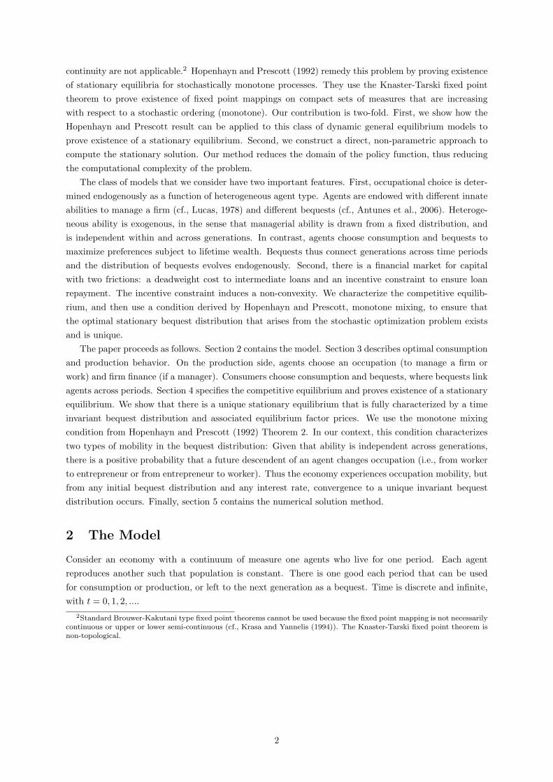
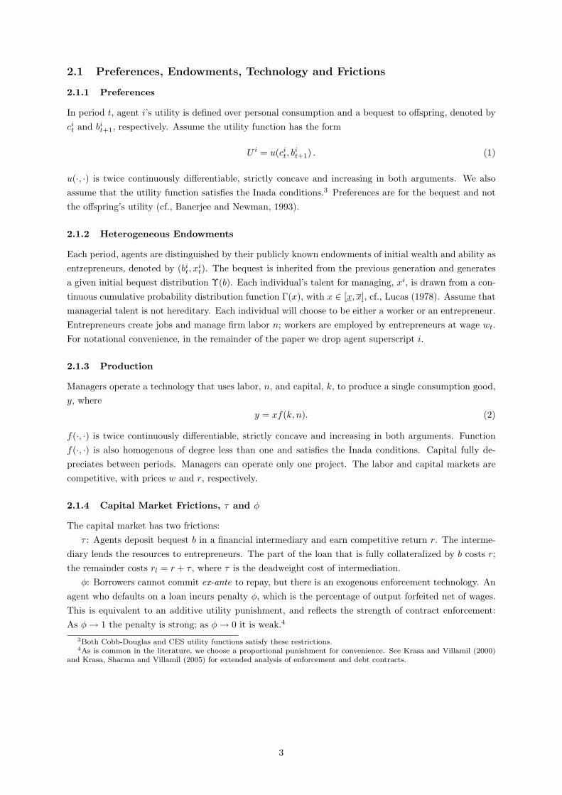
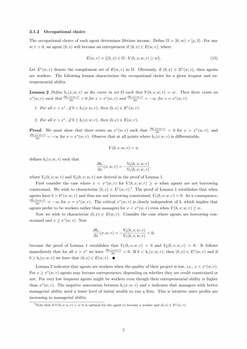
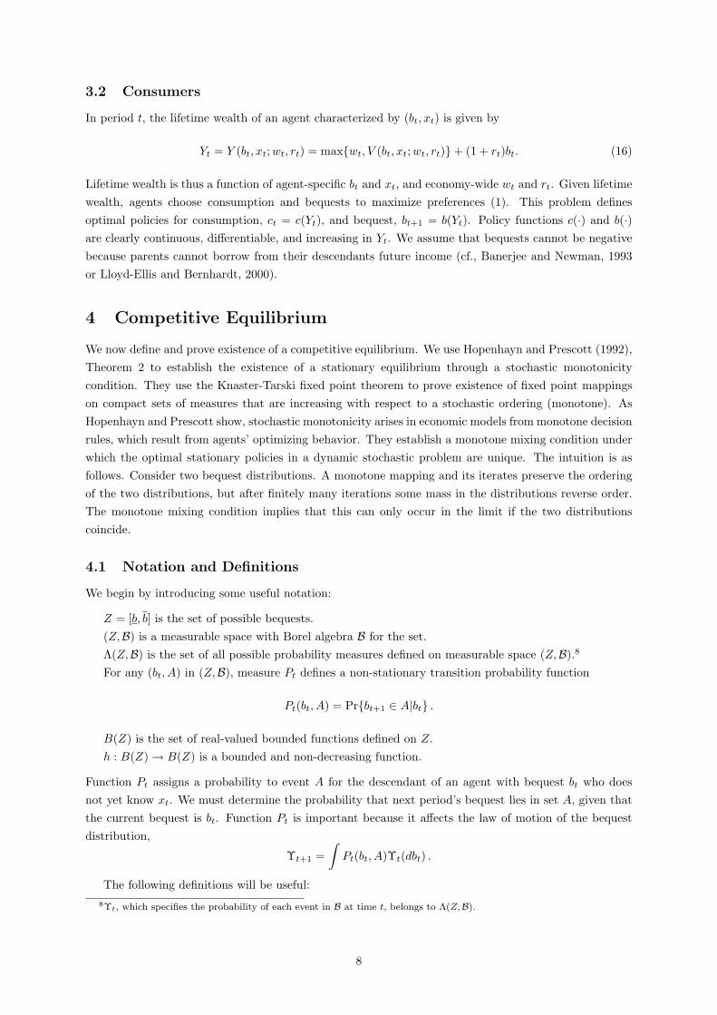
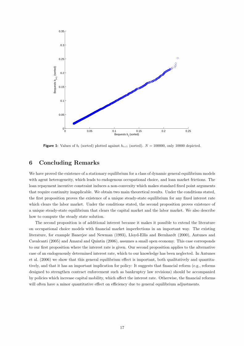
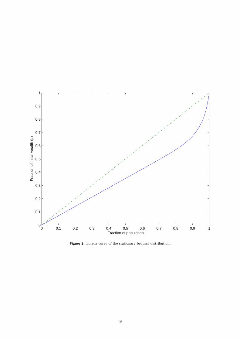
Figure 1 presents the sorted bequests in two consecutive periods plotted against each other. The curveis approximately a straight line, as expected. From this we see that the distribution is stable. The shapeof the stationary bequest distribution is depicted in Figure 2. The straight section is a consequence ofthe uniform wage rate.

18This does not imply that an agent always gets the same bequest.19In our case, Xt is bt and Wt is xt.

16

0 0.05 0.1 0.15 0.2 0.250

0.05

0.1

0.15

0.2

0.25

0.3

0.35

Bequests bt (sorted)

Beq

uest

s b t+

1 (so

rted

)

Figure 1: Values of bt (sorted) plotted against bt+1 (sorted). N = 100000, only 10000 depicted.

6 Concluding Remarks

We have proved the existence of a stationary equilibrium for a class of dynamic general equilibrium modelswith agent heterogeneity, which leads to endogenous occupational choice, and loan market frictions. Theloan repayment incentive constraint induces a non-convexity which makes standard fixed point argumentsthat require continuity inapplicable. We obtain two main theoretical results. Under the conditions stated,the first proposition proves the existence of a unique steady-state equilibrium for any fixed interest ratewhich clears the labor market. Under the conditions stated, the second proposition proves existence ofa unique steady-state equilibrium that clears the capital market and the labor market. We also describehow to compute the steady state solution.

The second proposition is of additional interest because it makes it possible to extend the literatureon occupational choice models with financial market imperfections in an important way. The existingliterature, for example Banerjee and Newman (1993), Lloyd-Ellis and Bernhardt (2000), Antunes andCavalcanti (2005) and Amaral and Quintin (2006), assumes a small open economy. This case correspondsto our first proposition where the interest rate is given. Our second proposition applies to the alternativecase of an endogenously determined interest rate, which to our knowledge has been neglected. In Antuneset al. (2006) we show that this general equilibrium effect is important, both qualitatively and quantita-tively, and that it has an important implication for policy: It suggests that financial reform (e.g., reformsdesigned to strengthen contract enforcement such as bankruptcy law revisions) should be accompaniedby policies which increase capital mobility, which affect the interest rate. Otherwise, the financial reformswill often have a minor quantitative effect on efficiency due to general equilibrium adjustments.

17

0 0.1 0.2 0.3 0.4 0.5 0.6 0.7 0.8 0.9 10

0.1

0.2

0.3

0.4

0.5

0.6

0.7

0.8

0.9

1

Fraction of population

Fra

ctio

n of

initi

al w

ealth

(b)

Figure 2: Lorenz curve of the stationary bequest distribution.

18

References

Amaral, P. and Quintin, E. (2006), ‘A competitive model of the informal sector’. Forthcoming in Journalof Monetary Economics.

Antinolfi, G. and Huybens, E. (1998), ‘Capital accumulation and real exchange rate behavior in a smallopen economy with credit market frictions’, Economic Theory 12, 461–488.

Antunes, A. and Cavalcanti, T. (2005), ‘Start up costs, limited enforcement, and the hidden economy’.Forthcoming in European Economic Review.

Antunes, A., Cavalcanti, T. and Villamil, A. (2006), ‘The effect of financial repression & enforcementon entrepreneurship and economic development’, Working Paper, University of Illinois at Urbana-Champaign .

Banerjee, A. V. and Newman, A. F. (1993), ‘Occupational choice and the process of development’, Journalof Political Economy 101(2), 274–298.

Betts, C. and Bhattacharya, J. (1998), ‘Unemployment, credit rationing, and capital accumulation: atale of two frictions’, Economic Theory 12, 489–518.

Boyd, J. and Smith, B. (1998), ‘The evolution of debt and equity markets in economic development’,Economic Theory 12, 519–560.

Erosa, A. (2001), ‘Financial intermediation and occupational choice in development’, Review of EconomicDynamics 4(2), 303–334.

Hopenhayn, H. A. and Prescott, E. C. (1992), ‘Stochastic monotonicity and stationary distributions fordynamic economies’, Econometrica 60(6), 1387–1406.

Kehoe, T. and Levine, D. (1993), ‘Debt-constrained asset markets’, Review of Economic Studies 60, 865–888.

Krasa, S., Sharma, T. and Villamil, A. P. (2005), ‘Debt contracts and cooperative improvements’, Journalof Mathematical Economics 41, 857–874.

Krasa, S. and Villamil, A. P. (2000), ‘Optimal contracts when enforcement is a decision variable’, Econo-metrica 68, 119–134.

Krasa, S. and Yannelis, N. (1994), ‘An elementary proof of the Knaster-Kuratowski-Mazurkiewitz-Shapleytheorem’, Economic Theory 4(1), 467–471.

Lloyd-Ellis, H. and Bernhardt, D. (2000), ‘Inequality and economic development’, Review of EconomicStudies 67(1), 147–168.

Lucas, Jr, R. E. (1978), ‘Asset prices in an exchange economy’, Econometrica 46, 1429–1445.

Stachurski, J. (2005), Computing the distributions of economic models via simulation, Manuscript, Uni-versity of Melbourne.

Stokey, N. L. (1988), ‘Learning by doing and the introduction of new goods’, Journal of Political Economy96, 701–717.

Stokey, N. L. and Lucas, Jr, R. E. (1989), Recursive Methods in Economic Dynamics, Harvard UniversityPress, Cambridge, Massachusetts. With Edward C. Prescott.

19