DI

SC

US

SI

ON

P

AP

ER

S

ER

IE

S

Forschungsinstitut zur Zukunft der ArbeitInstitute for the Study of Labor

Occupational Status and Health Transitions

IZA DP No. 5482

February 2011

G. Brant Morefi eldDavid C. RibarChristopher J. Ruhm

Occupational Status

and Health Transitions

G. Brant Morefield University of North Carolina at Greensboro

David C. Ribar

University of North Carolina at Greensboro and IZA

Christopher J. Ruhm

University of Virginia, NBER and IZA

Discussion Paper No. 5482 February 2011

IZA

P.O. Box 7240 53072 Bonn

Germany

Phone: +49-228-3894-0 Fax: +49-228-3894-180

E-mail: iza@iza.org

Any opinions expressed here are those of the author(s) and not those of IZA. Research published in this series may include views on policy, but the institute itself takes no institutional policy positions. The Institute for the Study of Labor (IZA) in Bonn is a local and virtual international research center and a place of communication between science, politics and business. IZA is an independent nonprofit organization supported by Deutsche Post Foundation. The center is associated with the University of Bonn and offers a stimulating research environment through its international network, workshops and conferences, data service, project support, research visits and doctoral program. IZA engages in (i) original and internationally competitive research in all fields of labor economics, (ii) development of policy concepts, and (iii) dissemination of research results and concepts to the interested public. IZA Discussion Papers often represent preliminary work and are circulated to encourage discussion. Citation of such a paper should account for its provisional character. A revised version may be available directly from the author.

IZA Discussion Paper No. 5482 February 2011

ABSTRACT

Occupational Status and Health Transitions* We use longitudinal data from the 1984 through 2007 waves of the Panel Study of Income Dynamics to examine how occupational status is related to the health transitions of 30 to 59 year-old U.S. males. A recent history of blue-collar employment predicts a substantial increase in the probability of transitioning from very good into bad self-assessed health, relative to white-collar employment, but with no evidence of occupational differences in movements from bad to very good health. These findings are robust to a series of sensitivity analyses. The results suggest that blue-collar workers “wear out” faster with age because they are more likely, than their white-collar counterparts, to experience negative health shocks. This partly reflects differences in the physical demands of blue-collar and white-collar jobs. JEL Classification: I12, J24 Keywords: occupations, physical demands, health Corresponding author: G. Brant Morefield Department of Economics University of North Carolina at Greensboro P.O. Box 26170 Greensboro, NC 27402-6170 USA E-mail: gbmorefi@uncg.edu

* We thank participants of the “SES and Health Across Generations and Over the Life Course” conference, September 23-24, 2010, held in Ann Arbor, MI for helpful comments.

1 

Occupational Status and Health Transitions

Introduction

Empirical research shows that physically demanding jobs are related to lower levels of

health. However, these results provide little indication about why health differs across

occupations or about how such differences are generated. A particular gap in our knowledge

involves how occupations might affect the timing of health changes, especially transitions into

and out of poor health. Information on these linkages could improve our understanding of the

mechanisms that lead to the association between occupation and health. Towards this end, we

examine how an individual’s occupational history is related to the probability of transitioning

between health states. Specifically, we focus on how health transitions are related to employment

in blue-collar, white-collar, and service occupations; we also consider differentials related to the

physical demands of occupations.

Occupational status could have asymmetric effects on health transitions – for example,

some occupations may be associated with relatively high probabilities of downward movements

in health but without a corresponding increase in health improvements. Consider the extreme

case of irreversible health changes. Occupationally influenced health investments might protect

against or mitigate the likelihood that such shocks take place (and so reduce the probability of

downwards health transitions) but would have no effect once such shocks occur (and so would

be unrelated to the likelihood of health improvements). Alternatively, once an individual

experiences a negative (but not irreversible) health shock his occupation may hinder his ability to

offset these deleterious effects with investment. The estimation method employed below allows

for such asymmetric effects.

Using data on men’s occupational and health histories from the 1984 through 2007 waves

2 

of the Panel Study of Income Dynamics (PSID), we create summary histories of occupation and

health status over a five-year window and examine how these are related to health two years

later. Consistent with prior research, the health of blue-collar workers is found to decline with

age faster than that of white-collar workers. What is new, however, is that we further show that

this is a consequence of blue-collar employees having a greater likelihood of transitioning from

very good to bad health but with no difference in the relative probability that they move from

bad to very good health. Similarly, periods out of work or in service jobs predict relatively high

rates of negative health transitions without an offsetting rise in the relative likelihood of health

improvements. These findings suggest that differences in rates of negative health shocks play a

primary role in explaining age-related occupational gradients in health. These qualitative results

are robust to several sensitivity analyses are unlikely to reflect differential patterns of errors in

self-reports of health status. We also show that heterogeneity in occupation-related physical

demands may explain some of the observed patterns.

Conceptual Issues and Previous Literature

In models of health capital, individuals make health investments to optimize healthy time

available to work and earn income, and this health capital can be used in combination with or as

a substitute for financial and traditional human capital (Grossman, 1972; Muurinen and Le

Grand, 1985). The health capital framework is also informative when considering health

transitions, since the stock of health capital at a point in time depends on health in the prior

period, investment flows, predictable depreciation in the health stock and (with uncertainty),

stochastic shocks resulting from illness, accidents and the like.

This framework identifies several reasons why occupational status may be related to

health. First, persons in highly paid occupations have more ability to finance health investments

3 

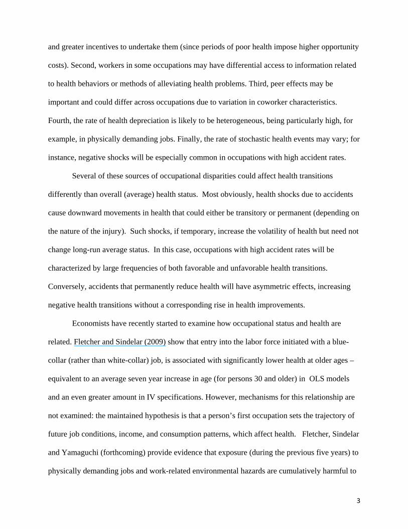
and greater incentives to undertake them (since periods of poor health impose higher opportunity

costs). Second, workers in some occupations may have differential access to information related

to health behaviors or methods of alleviating health problems. Third, peer effects may be

important and could differ across occupations due to variation in coworker characteristics.

Fourth, the rate of health depreciation is likely to be heterogeneous, being particularly high, for

example, in physically demanding jobs. Finally, the rate of stochastic health events may vary; for

instance, negative shocks will be especially common in occupations with high accident rates.

Several of these sources of occupational disparities could affect health transitions

differently than overall (average) health status. Most obviously, health shocks due to accidents

cause downward movements in health that could either be transitory or permanent (depending on

the nature of the injury). Such shocks, if temporary, increase the volatility of health but need not

change long-run average status. In this case, occupations with high accident rates will be

characterized by large frequencies of both favorable and unfavorable health transitions.

Conversely, accidents that permanently reduce health will have asymmetric effects, increasing

negative health transitions without a corresponding rise in health improvements.

Economists have recently started to examine how occupational status and health are

related. Fletcher and Sindelar (2009) show that entry into the labor force initiated with a blue-

collar (rather than white-collar) job, is associated with significantly lower health at older ages –

equivalent to an average seven year increase in age (for persons 30 and older) in OLS models

and an even greater amount in IV specifications. However, mechanisms for this relationship are

not examined: the maintained hypothesis is that a person’s first occupation sets the trajectory of

future job conditions, income, and consumption patterns, which affect health. Fletcher, Sindelar

and Yamaguchi (forthcoming) provide evidence that exposure (during the previous five years) to

physically demanding jobs and work-related environmental hazards are cumulatively harmful to

4 

health: a one standard deviation increase in physical demands is associated with a health

decrement for nonwhite men equivalent to a two-year reduction in schooling or four additional

years of age (with smaller effects for white males). Cross-sectional analyses for the U.S. (Case

and Deaton, 2005) and Canada (Choo and Denny, 2006) indicate that health depreciates faster

with age for individuals in manual than non-manual occupations, suggesting that occupations

have cumulative effects on health and alter its trajectory over the life course.

However, prior research does not examine how occupational status is related to health

transitions. The study of such transitions, which we undertake, is interesting in its own right and

potentially informative for understanding differences in age-related health gradients. As

discussed, blue-collar jobs are likely to have relatively high rates of accidents. These could result

in large but temporary deteriorations in health – implying relatively high probabilities of both

entering and exiting poor health – or permanent health decrements, so that blue-collar workers

disproportionately transition into but not out of poor health. Alternatively, downward mobility in

health might be similar across occupations, but blue-collar workers might have more difficulty

restoring good health, resulting in a relative deterioration for them at older ages. Our analysis

focuses on examining these potentially asymmetric health transitions across occupations. For the

most part, we will not explain why the transitions differ – that represents an important topic for

future research. However, we will provide some indication of the role played by the physical job

demands.

Methodology

We estimate dynamic models that allow us to examine how occupational status is

differentially (and possibly asymmetrically) associated with transitions from better to worse

health and vice versa. Let ht represent self-reported health status in year t for a given person.

5 

Most of our analyses consider a binary indicator where ht takes a value of one if the person

reports being in “good,” “fair,” or “poor” health (which we label below as “bad” health) and zero

if the person reports being in “very good” or “excellent” health (denoted as “very good” health).

have is average self-reported health measured over some previous period (t, t-2 and t-4 in most of

the analysis); OCCave is a vector that representing either occupational history over the five-years

ending in period t, or particular characteristics of that history; Xt is a vector of observed and

possibly time-varying personal characteristics; and εt is an error term that encompasses

unobserved characteristics. The basic model we estimate is described by:

θ γ β′X . (1)

In (1), estimated values of δ, θ, and γ indicate how health at time t+2 is related to the person’s

initial health status and occupational history.

Models that incorporate occupational histories have been estimated in previous studies;

however, our specifications further allow occupational status to have different associations with

transitions into and out of bad health. For people with a recent history of very good health, θ

describes how occupational status is associated with downwards health transitions. For people

with a history of bad health, δ, θ, and γ indicate how occupational status is associated with

movements into better health. The interpretations can be more complicated because have, which

averages health status over several years, can take values between zero and one.

We estimate (1) as a linear probability model throughout, for convenience and ease of

interpretation.1 The longitudinal design of the PSID provides the health and occupational history

                                                            1 Preliminary analysis revealed similar patterns of coefficients and statistical significance when using probit specifications, but the linear probability (LP) coefficients are easier to interpret, especially when including the occupation-health interactions (Ai and Norton, 2003).

6 

information needed to estimate the model but also leads to multiple observations for most of our

sample members. Therefore, the estimates below present robust standard errors clustered at the

individual level.

Data

Our data on men’s health and careers come from the Panel Study of Income Dynamics,

which began surveying “heads” and “wives” of a national sample of 4,800 families in 1968,

focusing on the economic and income behavior of the family.2 The PSID has followed these

families, including original sample members and their children when they establish independent

households. Interviews were conducted annually through 1997 and biennially thereafter.

In each panel since 1984, the PSID has asked heads and spouses: “Would you say your

health in general is excellent, very good, good, fair, or poor?” Self-reported overall health status

is a widely used summary measure that predicts subsequent mortality (Idler and Benyamini,

1997; Mossey and Shapiro, 1982) and is correlated with indicators of morbidity (Manor,

Matthews, and Power, 2001; Miilunpalo et al., 1997). While the measure has many advantages,

there are also limitations that should be kept in mind. One shortcoming that is relevant for

studies with employment outcomes is that self-reported health measures sometimes suffer from

“justification” bias – reporting health problems to explain poor labor force results (Currie and

Madrian, 1999). However, this bias is unlikely to depend upon the type of employment, unlike

self-reports of health-related work limitations, and the relationship between SHS and objective

health measures (like mortality) does not appear to vary between manual and non-manual

workers (McFadden et al., 2009).

                                                            2 Family “heads” are defined as the primary financial contributor to a PSID family, but defaults to the male partner of a female primary financial contributor if the male is a husband or has cohabited with the “wife” for at least a year.

7 

As described earlier, we dichotomize men’s SHS into “bad” health (SHS is good, fair, or

poor) and “very good” health (SHS is excellent or very good). Nearly our entire sample is

observed to be in very good or excellent health at least once. The use of “good” health as a cut-

off means that many of our sample members are also observed in the lower health category;

however, the results below are robust to using “fair” health as the dividing line.

We measure a person’s health history as a simple average of the binary health indicator

over the preceding five years (i.e., the proportion of surveys over a preceding five years when the

person reported “bad” health). To accommodate the PSID change to biennial surveying after

1997, our primary measure averages data from t, t – 2, and t – 4 (ignoring data from t – 1 and t –

3 that are available in some but not all years). For example, if the person reported bad health in

two of the three survey periods over the previous five years, the health history variable would

equal 0.667. As sensitivity tests, we investigated alternative health history variables including

one that contains data for all five years—including periods t – 1 and t – 3 when available—as

well as shorter three- and one-year histories. These changes did not alter our results.

Our analysis examines how occupational status and the physical demands of occupations

are associated with health transitions. To form the relevant measures, we consider reports

regarding the occupation of the main job held by the household head at the time of each

interview and the main job occupation held one year prior to the time of the interview in the

years when biennial surveys were conducted. The original 3-digit occupation codes were

reclassified, using the procedures detailed in Appendix A, to distinguish between “blue-collar,”

“white-collar” and “service” occupations, as well as periods of non-employment. These broad

occupational designations are assumed to capture some shared job characteristics, most

especially physical demands but also possibly work environments and autonomy in work

conditions. “White-collar” occupations mostly include jobs in offices, including managers and

8 

professionals, who often have a high degree of autonomy. The “blue-collar” occupations

generally include production work and tend to be more physically demanding. “Service”

occupations include some physically demanding jobs, such as protective service workers, but

also some positions with fewer physical demands, such as personal service workers. Blue-collar

and service workers generally enjoy less autonomy than white-collar workers.

These characterizations of positions are inexact. For example, the white-collar category

includes sales occupations, which might occur outside an office and involve little autonomy, and

the blue-collar category includes machine operators, who might have few physical demands.

Because of these issues, we also consider alternative classifications used in previous studies. In

some analyses, we follow Fletcher and Sindelar (2009) in considering differences between blue-

collar employees and all other workers (i.e., not distinguishing between white-collar and service

jobs). In other specifications, we follow Case and Deaton (2005) by considering managers and

professionals as one category and combining the remaining white-collar jobs with service

occupations into another category.

A more direct way to describe the conditions of employment is in terms of specific job

characteristics, rather than occupational groups. The core PSID interviews do not ask about these

characteristics; however, it is possible to map occupational codes to characteristics typical of

those occupations. We do this for one especially relevant characteristic—the physical demands

of the job. Using data from the Dictionary of Occupational Titles (DOT) and methods described

in Appendix A, occupations were classified on a five point scale where one indicates

“Sedentary” jobs and a five was assigned to those requiring “Very Heavy Work.” Consistent

with expectations, occupation-based physical demands were highest in blue collar jobs and

lowest in white collar occupations, with service employment being between the two–using the

five-point scale physical demands averaged 2.9, 2.5 and 1.6 for blue-collar, service, and white-

9 

collar workers in our sample.3

For our primary multivariate analyses, we measure the recent history of occupational

status or characteristics by taking the average of the relevant year-specific measures over the

preceding five years. For example, to describe the recent history of blue collar work, we create a

measure that represents the proportion of the previous five years that the person was employed in

a blue collar occupation. Similarly, to describe the recent physical demands, we take the average

of the physical demand measures over the last five years. In sensitivity analyses, we

experimented with slightly shorter and longer averaging windows and found that the results are

robust to these changes.

Our multivariate analyses include other relevant explanatory variables. A key

determinant of health is a person’s age, which we measure in years. To control for racial

differences in health, we include binary indicators for being black and for being neither black nor

white (the omitted category for these indictors is men who are white). Educational differences

are accounted for through binary indicators for: not completing high school, graduating high

school (or getting a GED) but without college, attending college but without obtaining a

bachelor’s degree, and completing a bachelor’s degree (or more education). We further

distinguish between men who were married and unmarried at the time of the survey and include

a general set of year dummy variables to account for trends in economic, social, health, and

policy conditions. The log of the family’s annual income is also included in some analyses.

Another issue arising in the PSID is that each year’s reports come from one respondent,

so that wives may sometimes be reporting the health status of their husbands. Our analyses

include a binary indicator for such proxy reporting. We have also conducted analyses that were

                                                            3 The physical demands variable should be interpreted cautiously because the measure averages some jobs within a three-digit occupational category, because the measure is ordinal rather than cardinal, and because occupational characteristics change over time.

10 

limited to men who were respondents with no substantial change in the results.

Our initial sample is restricted to 30 to 59 year-old male heads of households observed

after the PSID started collecting the self-reported health status information. The lower end of this

age restriction allows us to examine occupational effects after individuals have had time to amass

appreciable work histories. At the upper end, we stop our observations before most people retire

but after most have experienced at least some bad health. Indeed, 79 percent of our sample is

reported to be in bad health at least once during the observation period. Our observations are

further limited to years in which the men report not being in or having recently served in the

armed forces. Finally, we restrict the sample to observations with complete information for

seven-year span of health data (from t-4 to t+2) and the other explanatory measures. The final

principal analysis sample includes 34,607 person-years of information from 5,611 men. The

absence of females from our analysis represents a significant limitation that partially results from

the less complete data typically available for them but represents an important topic for future

research.

Descriptive Analyses

Table 1 lists the means for our analysis variables for all of the person-year observations

in our sample and conditionally for men reporting different health histories and transitions.

Thirty-nine percent of the person-year observations occurred in years where the men reported

being in bad health. When we consider the men’s recent histories of bad health (the average from

t, t – 2, and t – 4), the proportion of recent years of bad health drops slightly to 36 percent, which

is consistent with health gradually worsening with age.4 Our sample is composed mostly of

                                                            4 Other things held constant, there is a smaller chance that the men will be in bad health four years prior to the current interview year than in the interview year itself.

11 

observations for white-collar workers (44 percent) and blue-collar workers (39 percent), with

relatively few observations of service workers (6 percent) or non-working men (11 percent). The

demographic composition reflects the initial design of the PSID, which oversampled poor

households in its first sample in 1968. In particular, black men are over-represented and males

who are neither black nor white are under-represented. The average age is 42 years, and more

than five-sixths of the observations are of married men. The sample includes men with a range of

educational attainments.

Considering health status in periods t and t + 2, approximately half of the observations

represent continuations of very good self-reported health (16,893 out of 34,607), just over a

quarter of the observations come from continuations of bad health, leaving a quarter that

represent transitions between the health states. Thus, while changes in reported health status are

less frequent than continuations, there are still a substantial number of transitions. In particular,

there were 4,359 transitions from very good health to bad health, which implies a transition rate

of 21 percent, and 3,605 transitions from bad health to very good health, which implies a

transition rate of 27 percent.

Several occupational associations are also apparent in Table 1. Men with recent histories

of blue-collar work are under-represented in the observations with continuations of good health

but over-represented in other health patterns. This indicates that blue-collar work is associated

with a higher rate of transitioning to bad health and with being in bad health but not with moving

into very good health. In contrast, white-collar workers are over-represented in the observations

with continuations of very good health and under-represented in those with continuations of bad

health. The pattern suggests that white-collar workers have lower rates of transitioning into bad

health and higher rates of moving into very good health. The representation of service workers

does not vary substantially across the transition groups, suggesting that service jobs are not

12 

strongly associated with health or health transitions. The pattern of results for the recent histories

of physically-demanding jobs is consistent with those for the broad occupational categories.

Workers continuing in very good health had the least physically-demanding recent job histories;

those continuing in bad health had the most physically-demanding employment histories. In the

next section of the paper, we re-examine these relationships using multivariate models that

account for possible confounding influences of other observed characteristics.

Multivariate Results

In the following, we discuss the estimated effects of occupational history on the

probability of transitioning into and out of bad health from a history of very good and bad health,

respectively. Estimates from four linear probability specifications are reported in Table 2. As

described in equation (1), each includes controls for the recent health history, the recent

occupational history (the proportion of years working in blue-collar jobs, service jobs, and not

working), and interactions of the health and occupational histories. All of the models also control

for age, race, marital status, and general year effects, although for brevity, we only report the

coefficients for age. All columns except for the second also hold constant educational

attainment. The third and fourth columns also control for household income, with the last column

also adding occupation-specific age profiles.

In these specifications, the coefficients on the uninteracted occupational measures can be

directly interpreted as the conditional associations of occupational status with transitions from

very good health to bad health. The corresponding associations of occupational status with

transitions in the other direction, from bad health to very good health, can be determined by

combining the coefficients on recent health status, recent occupational histories, and their

interactions. While these coefficients are reported, we have also combined the relevant

13 

coefficients into summary measures of how of occupational status predicts transitions into very

good health. These are reported in the bottom panel of Table 2.

The estimates from the multivariate specifications are broadly consistent with

occupational differences in health transitions from the descriptive analyses. In the specification

reported in the first column with educational controls but no income controls, men whose recent

experience has been entirely in blue-collar work are estimated to face a 4.8 percent greater

chance of transitioning from very good to bad health than men whose recent experience has been

entirely in white-collar work. Men whose recent expericence has been entirely in service work

rather than white-collar also face higher rates of transitions into bad health, as do men who have

not been employed over the preceding five years.5

Estimates of the occupational differences in probabilities of transitioning between bad

and very good health (which are calculated by taking the negative of the sum of the interacted

and uniteracted occupational effects) are reported are reported in the lower panel of Table 2.

Results from the specification in the first column indicate that the probabilities of exiting bad

health for men with histories of blue-collar and service work do not differ significantly from the

probabilities for those with histories of white-collar work. However, men in bad health who have

not been employed appear to be less likely to transition back to very good health than other men.

These patterns of results are robust when we alter the controls in the models. The relative

probabilities of downwards health transitions for blue-collar, service and nonemployed workers

become stronger compared to those in white-collar jobs when education is excluded from the

model (column 2). There are also changes in the estimated occupational differences in the

probabilities of transitioning from bad health to very good health, although there are no changes                                                             5 The estimated effect of non-employment is difficult to interpret for two reasons. First, non-employment is highly endogenous to self-reported health for men in the sample age range (Currie and Madrian, 1999). Second, for observations with any observed non-employment (in the previous five years), fewer than 5 percent are non-employed for more than half of the period.

14 

in the statistical significance of the results. Positive correlations between education and health

have been widely observed (Grossman and Kaestner, 1997), and it seems likely that schooling

provides some protection against downwards movements in health. Given that education is

correlated with occupational status, it is not surprising that the predicted occupational effects on

negative health transitions become stronger when deleting education controls. Because the

general implications do not change when excluding education as a covariate, we follow the

previous empirical economics literature and control for education in all other specifications.

The third column of Table 2 lists results from a specification that adds the log of total

household income in period t as a control variable.6 The estimated occupational differences in

the probability of transitioning from very good health to bad health are slightly smaller than the

estimated differences in the first column. Men with a history of blue-collar employment are still

4.3 percentage points more likely to move from very good to bad health, relative their white-

collar counterparts. Similarly, the estimated difference for men with a work history in service

jobs is relatively close to the original estimate, at an increase of 3.0 percentage points in the

probability of entering bad health. As for exiting bad health, there are still no statistically

significant differences between men with blue-collar or service occupational histories and those

in white-collar jobs, while the differential associated with non-employment shrinks in size and

loses statistical significance. In general, results from this specification indicate that income plays

a partial mediating role between occupational status and health outcomes but that other sizeable

associations still remain.

Specification (4) adds interactions between the employment history variables and a linear

age trend, allowing health trajectories to differ with age across occupational types. If

occupational status is associated with the general age profile of health, we might expect to see

                                                            6 We have also used total household income averaged over the 5-year period without a substantive change in results.

15 

differences in these interactions rather than the transition terms. However, the interactions

between occupational status and age are not statistically significant and occupational differences

continue to appear in health transitions.

Sensitivity Tests

We have re-estimated our models using several alternative specifications of our health

and occupational history measures. Selected results from these alternative specifications are

reported in Table 3. The specifications in Table 3 generally have the same auxiallary controls as

the first specification in Table 2 (i.e., they include controls for age, race, marital status, proxy

reporting, education, and year effects but omit controls for income or occupation-specific age

effects). Table 3 reports coefficients on the differences between workers in blue-collar and

white-collar occupations in their transitions into and out of bad health.

The first three specifications in Table 3 incorporate alternative measures of our health

history variable. Recall that for reasons of consistency over different years of the PSID, our

recent health history measure includes observations from periods t – 4, t – 2, and t but not

periods t – 3 or t – 1, even when those observations are available. The initial specification in

Table 3 includes all of the available observations in the health history measure. However, there is

almost no change in the estimated results.

In the next two rows, we report results from models that use different reporting lengths to

define the person’s initial health status. One reason for combining several years of health data

into a single summary measure is to reduce some of the noise associated with the wave-to-wave

measures. However, the resulting summary measure may introduce problems of its own by

including health reports from several years ago that may not be relevant at the time of the

interview. Also, if an individual is in bad health for the full time of the five-year window, it may

16 

be the case that the health persistence is too strong to identify any differences across

occupational types. To investigate differing health histories, we consider two specifications that

use shorter health history measures: one specification uses data from periods t – 2 and t, while

the other uses information only from period t. Our findings remain robust. The estimated

differences between the probabilities of blue-collar and white-collar workers transitioning to bad

health become slightly stronger when we condition on shorter histories of health. The estimated

differences in the probabilities of transitioning to very good health do not change. The change in

relative probability of transitioning into but not out of bad health provides evidence against one

concern of this study, occupationally related measurement error in self-reported health status. If

the level of measurement error in self-reported health, uninformative movement between health

categories, is greater for individuals in blue-collar occupations then we might expect to see

greater probabilities of transitioning between better and worse health states when we condition

on shorter measures of health history for this group. The fact that we see a greater probability of

transitioning into bad health but no change in the probability of transitioning out of that status

when the shorter health history measures are used suggests that differences in the probability of

transitions are not simply due to the correlation of measurement error in the health variable with

occupational types.

The next row in Table 3 lists results from a specification that defines “bad” health at a

different point in the SHS scale. In particular, we re-specify the cut-off for bad health more

stringently as reporting “fair” or “poor” SHS, rather than “good,” “fair,” or “poor.” Even with

the stricter definition, blue-collar workers are estimated to face a higher risk of a negative health

transition than white-collar workers. Consisent, however, with the lower overall probability of

experiencing “fair” or “poor” health, the size of the differential is reduced from our previous

specifications. The differences between blue-collar and white-collar workers in their

17 

probabilities of transitioning to better health remain statistically insignificant but mainly due to

an imprecise estimate.

The fifth row of Table 3 lists results from a specification that uses bad health in either

period t + 2 or t + 4 as the dependent variable, rather than bad health in only period t + 2. The

additional time to switch health states increases the differences between white-collar and blue-

collar work histories in the probability of entering bad health from very good health. Yet, there

is still no discernable difference between the probability of exiting bad health for men with blue-

and white-collar work histories.

The remaining rows of Table 3 report results from models that use alternative

occupational history measures and contrasts. The first of these specifications drops the controls

for service occupations. This has the effect of combining service workers and white-collar

workers into a single (omitted) category. A similar contrast was examined by Fletcher and

Sindelar (2009) in their study of initial occupational choices. The change in the occupational

measures has almost no effect, however, on the estimated associations. The stability of the

estimates most likely results from the very low incidence of service work in our sample.

In the seventh row of Table 3, we list estimates from a model that combines service,

sales, and administrative workers into a single occupational category. Thus, the omitted

occupational group in the models becomes a narrower group of professional and managerial

workers. Once again, however, there are few substantive changes in the results.

The final row in Table 3 lists results from a regression that replaces the blue-collar and

service occupational measures with the five-year average physical demands variable. The results

confirm the previous findings that more manual occupations are related to a greater probability

of transitioning into bad health given a history of very good health and no significant difference

in the probability of transitioning into better health from bad health.

18 

The variables for occupational histories and physical demands are measured in different

units; however, it is possible to make a rough comparison of the estimated effects. The average

physical demands of a blue-collar occupation in our sample are 1.3 units greater than the average

physical demands of a white-collar occupation. If we apply this adjustment factor, five years of

employment with the average physical demands of a blue-collar job would increase the

probabilty of transitioning to bad health by 2.1 percentage points relative to employment with the

average physical demands of a white-collar job. The calculation indicates that physical demands

can account for almost half of the differential in transitions between very good and bad health

between blue- and white-collar workers.

Conclusion

We use longitudinal data on men’s health and occupational histories, from the PSID, to

examine how occupational status is asociated with health and health transitions. Previous

research indicates that health varies by occupation and that this heterogeneity increases with age.

However, since health does not not simply decline over the life-course—with both health

decrements and improvements occurring frequently—we estimate models that identify

relationships between occupational history and the probabilities of transitioning between both

better and worse health for U.S. working age males.

The results show that a recent (five year) history of blue-collar employment predicts a

four-to-five percentage point increase in the probability of moving from very good (“very good”

or “excellent”) into bad (“poor”, “fair”, or “good”) self-assessed health, relative to white-collar

employment. However, there are no indications that blue-collar work differentially affects the

probability of transitioning out of worse health. Education and income are positively related to

health, as in previous studies, but their inclusion does not eliminate the observed occupational

19 

effects.

These findings are robust to a series of sensitivity analyses and do not appear to reflect

errors in the reporting of self-assessed health. In particular, we estimate specifications that

shorten the measured health histories from five years to either three years or one year.

Conditioning on shorter health histories should increase measurement error, since averaging

occurs over fewer years, and is likely to then increase the likelihood of reporting error based

health transitions. Consistent with this, we do see a rise in the relative probability that blue-collar

workers transitions into poorer health when using shorter occupational histories. However, there

is no corresponding indication that they are more likely to move from bad to very good health, as

the differential reporting error explanation would predict.

Our findings suggest that blue-collar workers “wear out” faster with age because they

experience more negative health shocks than their white-collar counterparts. There is no

evidence that they have greater difficulty in recovering from given shocks, nor is there a strong

indication that they regain health more quickly or completely following them. Future research

could fruitfully examine mechanisms underlying this occupational heterogeneity. An obvious

possibility is that blue-collar workers are more prone to accidents or job-related physical

traumas. Indeed, our analysis suggests that physical job demands can account for around two-

fifths of the difference in the transition rates of blue-collar versus white-collar workers.

Important caveats should be kept in mind when interpreting our results. Most

importantly, endogeneity could be problematic if workers with histories of blue-collar

employment have faster health declines than those in white-collar occupations for reasons that

are not occupationally related or observed. The inclusion of additional covariates and the use of

instrumental variables methods or other identification strategies in future work would be helpful

for examining the consequences of such occupational selection. Second, dichotomization of self-

20 

reported health status limits our findings to a subjectively chosen threshold and implies that we

potentially lose information about movements into or out of more extreme health states. Third,

during an era when female employment rates are approaching or exceeding those males and the

occupations in which they work are becoming increasingly diverse, an extension of this research

to consider women’s occupational histories should be pursued.

21 

References

Adams, P., M. Hurd, D. McFadden, A. Merrill, and T. Ribeiro. (2003). “Healthy, wealthy, and

wise? Tests for direct causal paths between health and socioeconomic status.” Journal of

Econometrics 112, no. 1: 3-56.

Ai, Chunrong and Edward Norton. (2003) “Interaction Terms in Logit and Probit Models.”

Economics Letters. 80: 123-129.

Bureau of Labor Statistics. 2010. “Occupational and Wage Estimates.” Occupational

Employment Statistics. United States Department of Labor. Accessed 7 Dec. 2010.

<http://www.bls.gov/oes/oes_dl.htm >

Callegaro, Mario. (2007). “Seam Effects Changes Due to Modifications in Question Wording

and Data Collection Strategies: A Comparison of Conventional Questionnaire and Event

History Calendar Seam Effects in the PSID.” Ph.D. Dissertation. Lincoln, NE: University

of Nebraska.

Case, Anne and Angus Deaton. (2005). “Broken down by work and sex: How our health

declines.” In Analyses in the economics of aging, ed. David A. Wise:185-205: Chicago:

University of Chicago Press.

Chao, Elaine L. and Kathleen P. Utgoff. (2003). “National Compensation Survey: Occupational

Wages in the United States, January 2001.” US Department of Labor – Bureau of Labor

Statistics, Bulletin 2552.

Choo, Eugene and Michael Denny. (2006).” Wearing out--the decline in health.” 28 pages:

University of Toronto, Department of Economics, Working Papers.

Currie, Janet and Brigitte C. Madrian. (1999). “Health, health insurance and the labor market.” In

Handbook of labor economics. Volume 3c, ed. Orley Ashenfelter and David Card:3309-

22 

3416: Handbooks in Economics, vol. 5. Amsterdam; New York and Oxford: Elsevier

Science, North-Holland.

Fletcher, Jason M. and Jody L. Sindelar. (2009). “Estimating causal effects of early occupational

choice on later health: Evidence using the psid.” NBER Working Paper #15256.

Fletcher, Jason M., Jody L. Sindelar, and Shintaro Yamaguchi. (Forthcoming). “Cumulative

effects of job characteristics on health.” Health Economics.

Grossman, Michael. (1972). “On the concept of health capital and the demand for health.”

Journal of Political Economy 80, no. 2: 223-55.

Grossman, Michael and Robert Kaestner. (1997). “Effects of education on health.” In The social

benefits of education, ed. Jere R. Behrman and Nevzer Stacey:69-123: Economics of

Education series. Ann Arbor: University of Michigan Press.

Idler, Ellen L. and Yael Benyamini. (1997). “Self-Rated Health and Mortality: A Review of

Twenty-Seven Community Studies.” Journal of Health and Social Behavior. Vol. 38(1):

21-37.

Manor, Orly, Saron Matthews, and Chris Power. (2001). “Self-rated health and limiting

longstanding illness: inter-relationships with morbidity in early adulthood.” International

Journal of Epidemiology. Vol. 30(3): 600-607.

McFadden, Dan. (2005). “Comments on case and deaton 'broken down by work and sex: How

our health declines'.” In Analyses in the economics of aging, ed. D. Wise:205-212.

Chicago: University of Chicago Press.

McFadden, E., R. Luben, S. Bingham, N. Wareham, A.-L.Kinmonth, and K.-T. Chaw. (2009)

“Does the association between self-rated health and mortality vary by social class?”

Social Science & Medicine 68. no. 2: 275-280.

Miilunpalo, Seppo, Ilkka Vuori, Pekka Oja, Matti Pasanen, and Helka Urponen. (1997). “Self-

23 

Rated Health Status as a Health Measure: The Predictive Value of Self-Reported Health

Status on the Use of Physician Services and on Mortality in the Working-Age

Population.” Journal of Clinical Epidemiology. Vol. 50(5): 517-528.

Mossey, J.M. and E. Shapiro. (1982). “Self-rated health: A predictor of mortality among the

elderly.” American Journal of Public Health 72, no. 8: 800-808.

Muurinen, Jaana-Marja and Julian Le Grand. (1985). “The economic analysis of inequalities in

health.” Social Science & Medicine 20, no. 10: 1029-1035.

24 

Table 1: Sample Statistics of Selected Variables

Sample: Health (t, t +2) Full Sample Bad(0,0) Bad(0,1) Bad(1,1) Bad(1,0) Health

"Bad" health in period t 0.386 - - 1 1 (0.006) - - - - Recent history of bad health 0.364 0.081 0.243 0.818 0.605

(0.005) (0.002) (0.004) (0.004) (0.005) Recent occupational history

Blue-collar 0.386 0.335 0.452 0.423 0.445 (0.007) (0.008) (0.010) (0.010) (0.010)

White-collar 0.444 0.555 0.398 0.278 0.389 (0.007) (0.009) (0.010) (0.007) (0.010)

Service job 0.063 0.062 0.070 0.076 0.070 (0.003) (0.004) (0.005) (0.005) (0.005)

Not employed 0.107 0.049 0.081 0.222 0.096 (0.003) (0.002) (0.005) (0.008) (0.006)

Physical Demands 2.232 2.104 2.315 2.417 2.317 (Employed only) (0.004) (0.014) (0.016) (0.017) (0.017)

Individual Characteristics

White 0.707 0.800 0.657 0.589 0.650 (0.007) (0.008) (0.010) (0.012) (0.011)

Black 0.261 0.173 0.312 0.373 0.311 (0.007) (0.007) (0.010) (0.012) (0.011)

Other race 0.032 0.027 0.031 0.038 0.038 (0.002) (0.003) (0.003) (0.003) (0.004)

Age 42.3 41.2 42.1 44.3 42.1 (0.096) (0.123) (0.147) (0.162) (0.158)

Less than HS 0.136 0.062 0.160 0.243 0.167 (0.005) (0.004) (0.008) (0.011) (0.009)

HS graduate 0.366 0.324 0.392 0.413 0.401 (0.008) (0.010) (0.011) (0.012) (0.011)

Some college 0.228 0.243 0.232 0.199 0.226 (0.007) (0.009) (0.009) (0.010) (0.009)

Bachelor's degree 0.270 0.371 0.215 0.145 0.206 (0.007) (0.010) (0.009) (0.009) (0.009)

Married 0.860 0.881 0.852 0.820 0.854 (0.004) (0.005) (0.007) (0.008) (0.007)

Household income 70894 84816 64838 51600 64697 (997) (1649) (1044) (889) (1121)

Person-years n =

34,607 16,893 4,359 9,750 3,605

Note: Table shows the average values of selected characteristics for a sample of 5,611 30-59 year old men in the Panel Survey of Income Dynamics, 1988-2005. Clustered standard errors are in parentheses.    

25 

Table 2. Selected Results from Linear Probability Models of the Probability of “Bad” Health

(1) (2) (3) (4)

Recent history of bad health 0.718*** 0.728*** 0.714*** 0.719*** (0.012) (0.012) (0.012) (0.012)

Blue-collar occupation 0.048*** 0.075*** 0.043*** 0.037*** (0.009) (0.008) (0.009) (0.012)

Service occupation 0.036* 0.057*** 0.030* 0.011 (0.016) (0.016) (0.016) (0.022)

Not employed 0.127*** 0.150*** 0.096*** 0.136*** (0.025) (0.025) (0.025) (0.028)

Blue-collar occupation × -0.060*** -0.059*** -0.060*** -0.064*** recent history of bad health (0.017) (0.016) (0.017) (0.017) Service occupation × -0.018 -0.020 -0.020 -0.028 recent history of bad health (0.027) (0.028) (0.027) (0.029) Not employed × -0.073** -0.069** -0.069** -0.066** recent history of bad health (0.029) (0.029) (0.028) (0.030) Age 0.003*** 0.003*** 0.003*** 0.002***

(0.000) (0.000) (0.000) (0.001) Blue-collar*Age 0.001

(0.001) Service*Age 0.002

(0.002) Not employed*Age -0.001

(0.001) Additional Controls Education Yes No Yes Yes Household Income No No Yes Yes

Calculated associations of characteristics with transitions to very good health Blue-collar occupation 0.012 -0.016 0.017 0.027 (0.014) (0.013) (0.014) (0.019) Service occupation -0.017 -0.037 -0.010 0.018 (0.022) (0.021) (0.022) (0.032) Not employed -0.054*** -0.081*** -0.027 -0.070*** (0.015) (0.015) (0.015) (0.025) Note: Table displays coefficients from linear probability models where the dependent variable is "bad" health in period t+2. The models were estimated using 34,607 person-year observations on 5,611 men from the 1988-2005 waves of the PSID. All models include controls for race, marital status, proxy respondents, and general year effects. The coefficients for the transitions to very good health are the calculated by combining the coefficients for health and occupational histories and their interactions. Robust standard errors, clustered by individual, are shown in parentheses.

Table 3. Predicted Difference in Probability of Health Transitions for Blue-collar Versus White-collar Occupations

Econometric Specification Transition to Worse Health Status Transition to Better Health Status

(1) Health History included in 0.042*** 0.015 all available years (0.009) (0.014)

(2) Health History in t & t-2 0.055*** 0.004 Only (0.010) (0.014)

(3) Health History in t only 0.066*** -0.008 (0.011) (0.015)

(4) Restrictive Definition of 0.015*** 0.012 “Bad” Health (0.004) (0.040)

(5) Health Transition in 0.081*** 0.019 t+2 or t+4 (0.014) (0.019)

(6) Blue-collar vs other occupation 0.041*** 0.018 (0.009) (0.013)

(7) Blue-collar vs professional 0.051*** 0.011 (0.010) (0.016)

Non-blue-collar vs professional 0.026*** -0.011 (0.010) (0.020)

(8) Physical demands 0.016*** 0.004 (0.0053) (0.0015)

Note: Specifications in rows (1)-(5) show the difference in the predicted probability of transitions into or out of bad health for men with a 5-year history of blue-collar work versus an equal period in white-collar work. Specifications in rows (6)-(8) show the difference in the predicted probability of transitions into or out of bad health for men with a 5-year history in the listed occupations. The coefficients are from linear probability models estimated using 34,607 person-year observations for 5,611 men from the 1988-2005 waves of the PSID. All models include controls for race, educational attainment, marital status, proxy respondents, and general year effects. Model (1) includes health history variables in years t-1 and t-3 in all years these are available. Models (2) and (3) measure health history over shorter time periods, and specification (5) models bad health that occurs in either t+2 or t+4. Specification (8) refers to a one-point change in the physical demands score over five years. Robust standard errors, clustered by individual, are shown in parentheses.

Appendix A: Occupational Classifications

The PSID provided 3-digit 1970 Census group definitions for the 1984 through 2001

waves and 3-digit 2000 Census group definitions for the 2003 and later surveys. To make this

information uniform for all survey rounds, we recoded the occupation codes to 1990 Census

definitions for all years using the crosswalk provided by IPUMS-USA

(http://usa.ipums.org/usa/volii/documents/occ1990_xwalk.xls). The occupations were

subsequently defined as “blue-collar,” “white-collar,” or “service” following listings provided by

the Bureau of Labor Statistics (Chao and Utgoff, 2003). Twenty-six occupations were not

included in the BLS list; we have categorized these occupations within the classification that is

subjectively appropriate. A list of the classifications appears in Table A-1. In addition to the

occupational classifications, we also include a fourth category for people who were not

employed at the time of the survey.

There are two notes of interest in constructing these categorical variables. First, the PSID

identifies individuals serving in the armed forces but does not indicate their occupation while in

military service. Since there were too few observations to classify military service as a separate

occupation, we dropped person-year observations for individuals serving in the armed forces

during the 5-year occupational history window. Second, a small number individuals report being

unemployed or out of the labor force but still indicate an occupation. For consistency, we coded

these individuals as not-employed.

Our main occupation variables represent average values for over the five years t-4, t-3, t-

2, t-1, and t. In the years up to 1997, we used information on the occupation of the primary job at

the time of the interview for all of these periods. In years after 1997, when the PSID interviewed

biennially, we used available retrospective work history information to identify the occupation of

28  

individuals in the month one year prior to the survey month to obtain the measures for periods t-

3 and t-1. For instance, an individual’s 1998 occupation is defined as that reported in the month

one year prior to the 1999 interview.7 If data were missing for any years between t-4 and t (after

including the constructed values just discussed), averaging took place over the period for which

the data were available.

We merged onto the dataset information on the physical demands of occupations using

data from the Dictionary of Occupational Titles (DOT): Revised Fourth Edition (1991), which

provides a five point ordinal measure of the physical demands for 12,742 occupations. The

demands are listed as Sedentary, Light Work, Medium Work, Heavy Work, and Very Heavy

Work (see http://www.occupationalinfo.org/appendxc_1.html#STRENGTH).

We matched the physical demand characteristics of DOT occupations to the Census

occupational codes by coding the five measures to integers, one to five, increasing in physical

demands. The DOT occupations and physical demand scores were then matched to Occupational

Employment Statistics (OES) codes provided by the Bureau of Labor Statistics (BLS Crosswalk

Center) and averaged over the DOT occupations within each OES occupation. Finally, physical

demands by OES occupation were weighted according to 1997 estimates of the number of

individuals employed in each of the OES occupations (BLS, 2010) and matched to the 1990

Census occupation codes for person-years in our PSID data set.

                                                            7 The retrospective information in the non-interview years (1998, 2000, 2002, 2004, and 2006) provides fewer occupational transitions than interview years. A lower proportion of transitions during the recalled employment history is consistent with seam effects, which have been found in the employment history of the PSID. However, occupational measures during the non-interview years match the characteristics of those during interview years in the terms of the number of observations and proportion of individuals in each occupational state (Callegaro, 2007).

Table A-1. Classification of occupations White-collar Professional Specialty & Technical Occupations (043-235), n = 5850 Executive, Administrative, & Managerial Occupations (003-37), n = 6975 Sales Occupations (243-85), n = 2334 Administrative Support Occupations (303-48, 353, 356-89), n = 1767 Classified by the Authors

Other Telecom Operators (349), n = 1 Postal Clerks, Excluding Mail Carriers (354), n = 138 Managers, Farms, Except Horticultural (475), n = 109

Blue-collar Precisions Production, Craft, & Repair Occupations (503-29, 534-47, 553-654, 656-58, 666-69, 675-99), n = 6451 Machine Operators, Assemblers, & Inspectors (703-14, 723-24, 726-29, 734-36, 738-48, 753-77, 783-800), n = 1927 Transportation and Material Moving Occupations (803-59), n = 3059 Handlers, Equipment Cleaners, Helpers, and Laborers (483-87, 489, 864-89), n = 1870 Classified by the Authors

Farmers, Except Horticulture (473), n = 420 Farm Workers (477,479), n = 310 Graders and Sorters, Agricultural Products (488), n = 4 Miscellaneous Electrical and Electronic Equipment Repairers (533), n = 4 Not Specified Mechanics and Repairers (549), n = 317 Miscellaneous Woodworking Machine Operators (733), n = 5 Miscellaneous Textile Machine Operators (749), n = 63 Machine operators, not specified (779), n = 869

Service Jobs Protective, Food, Health, Cleaning, and Personal Service (413-69), n = 2438 Classified by the Authors

Mail Carriers, Postal Service (355), n = 164 Housekeepers and Butlers (405), n = 141 Private Household Cleaners and Servants (407), n = 8

NOTE: Groups are based on 1990 3-digit Census occupation codes in parentheses. Blue-collar, white-collar, and service job classifications are based on the work of Chao and Utgoff (2003) except for occupations “Classified by the Authors,” which were classified for use in this paper only. The numbers of observations, n, refer to person-year observations between 1984 and 2005.