Filament Estimation and Uncertainty Measures
90
Filament Estimation and Uncertainty Measures Yen-Chi Chen Larry Wasserman Christopher Genovese Jessi Cisewski Peter Freeman Shirley Ho Jiashun Jin Alessandro Rinaldo Department of Statistics Carnegie Mellon University April 21, 2014 1 / 39
Transcript of Filament Estimation and Uncertainty Measures

Filament Estimation and Uncertainty Measures
Yen-Chi Chen
Larry Wasserman Christopher GenoveseJessi Cisewski Peter Freeman
Shirley Ho Jiashun Jin Alessandro Rinaldo
Department of StatisticsCarnegie Mellon University
April 21, 2014
1 / 39

Outline
Introduction to Filaments
Filament Estimation
Uncertainty Measures
Future Work
2 / 39

Introduction
Outline
Introduction to Filaments
Filament Estimation
Uncertainty Measures
Future Work
3 / 39

Introduction
Filaments Example: Astronomy
Credit: Millennium Simulation 4 / 39

Introduction
Filaments Example: Neuroscience
Image courtesy Eswar P. R. Iyer. 5 / 39

Introduction
Filaments Example: Earthquake
Credit: PhysicalGeography.net
6 / 39

Introduction
Filament Example: the real Universe
Credit: 2MASS.
7 / 39

Introduction
Focus of the Thesis: Point Data (from SDSS)
8 / 39

Introduction
Focus of the Thesis: Point Data (from SDSS)
8 / 39

Introduction
Focus of the Thesis: Point Data (from SDSS)
8 / 39

Introduction
Statistical Model for Filaments: Density Ridges
Formally, we define a filament to be a ridge of the density.
9 / 39

Introduction
Example: Ridges in Mountians
Credit: Google
10 / 39
Introduction
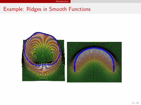
Example: Ridges in Smooth Functions
11 / 39

Introduction
Example: Ridges in Smooth Functions
12 / 39

Introduction
Example: Ridges in 3-D
13 / 39

Introduction
Example: Ridges in 3-D
13 / 39
Introduction
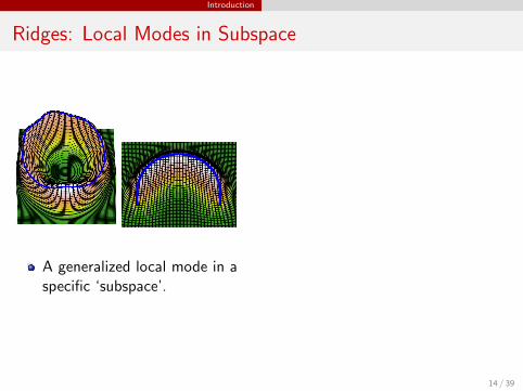
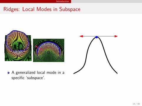
Ridges: Local Modes in Subspace
A generalized local mode in aspecific ‘subspace’.
14 / 39

Introduction
Ridges: Local Modes in Subspace
A generalized local mode in aspecific ‘subspace’.
14 / 39
Introduction
Ridges: Local Modes in Subspace
A generalized local mode in aspecific ‘subspace’.
14 / 39
Introduction
Definition of Density Ridges
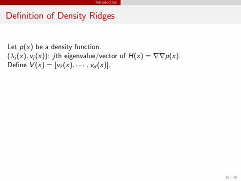
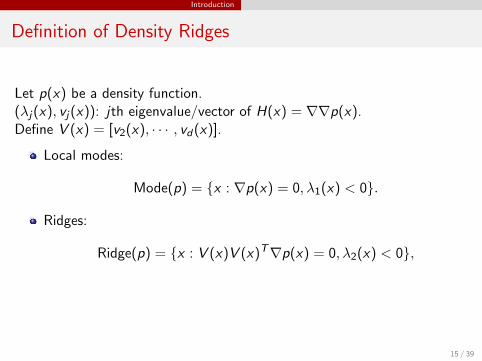
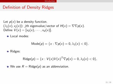
Let p(x) be a density function.(λj(x), vj(x)): jth eigenvalue/vector of H(x) = ∇∇p(x).Define V (x) = [v2(x), · · · , vd(x)].
Local modes:
Mode(p) = {x : ∇p(x) = 0, λ1(x) < 0}.
Ridges:
Ridge(p) = {x : V (x)V (x)T∇p(x) = 0, λ2(x) < 0},
We use R = Ridge(p) as an abbreviation.
15 / 39

Introduction
Definition of Density Ridges
Let p(x) be a density function.(λj(x), vj(x)): jth eigenvalue/vector of H(x) = ∇∇p(x).Define V (x) = [v2(x), · · · , vd(x)].
Local modes:
Mode(p) = {x : ∇p(x) = 0, λ1(x) < 0}.
Ridges:
Ridge(p) = {x : V (x)V (x)T∇p(x) = 0, λ2(x) < 0},
We use R = Ridge(p) as an abbreviation.
15 / 39

Introduction
Literature Review
Early work on ridges: image analysis[Hall et. al. (1991), Eberly (1996), Damon (1999)]
Algorithm: subspace constrainted mean shift[Ozertem and Erdogmus (2011)]
Theory: geometric and topological convergence[Genovese et. al. (2012)]
16 / 39

Current Progress: Filament Estimation
Outline
Introduction to Filaments
Filament Estimation
Uncertainty Measures
Future Work
17 / 39
Current Progress: Filament Estimation
Filament Estimator: Plug-in Estimate
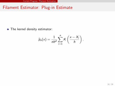
The kernel density estimator:
p̂n(x) =1
nhd
n∑i=1
K
(x − Xi
h
).
The estimated ridges:R̂n = Ridge(p̂n).
In practice, we throw aways points in low density regions.
18 / 39

Current Progress: Filament Estimation
Filament Estimator: Plug-in Estimate
The kernel density estimator:
p̂n(x) =1
nhd
n∑i=1
K
(x − Xi
h
).
The estimated ridges:R̂n = Ridge(p̂n).
In practice, we throw aways points in low density regions.
18 / 39

Current Progress: Filament Estimation
Filament Estimator: Plug-in Estimate
The kernel density estimator:
p̂n(x) =1
nhd
n∑i=1
K
(x − Xi
h
).
The estimated ridges:R̂n = Ridge(p̂n).
In practice, we throw aways points in low density regions.
18 / 39

Current Progress: Filament Estimation
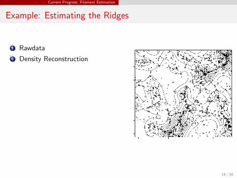
Example: Estimating the Ridges
1 Rawdata
2 Density Reconstruction
3 Thresholding
4 Ridge Recovery (Ozertem andErdogmus 2011)
19 / 39
Current Progress: Filament Estimation
Example: Estimating the Ridges
1 Rawdata
2 Density Reconstruction
3 Thresholding
4 Ridge Recovery (Ozertem andErdogmus 2011)
19 / 39

Current Progress: Filament Estimation
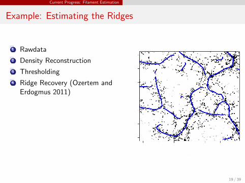
Example: Estimating the Ridges
1 Rawdata
2 Density Reconstruction
3 Thresholding
4 Ridge Recovery (Ozertem andErdogmus 2011)
19 / 39

Current Progress: Filament Estimation
Example: Estimating the Ridges
1 Rawdata
2 Density Reconstruction
3 Thresholding
4 Ridge Recovery (Ozertem andErdogmus 2011)
19 / 39
Current Progress: Filament Estimation
Example: Estimating the Ridges
1 Rawdata
2 Density Reconstruction
3 Thresholding
4 Ridge Recovery (Ozertem andErdogmus 2011)
19 / 39

Current Progress: Filament Estimation
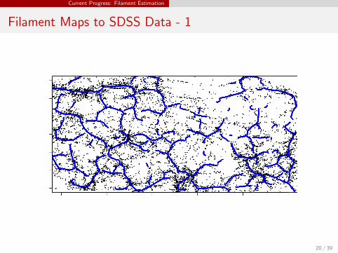
Filament Maps to SDSS Data - 1
20 / 39
Current Progress: Filament Estimation
Filament Maps to SDSS Data - 1
20 / 39

Current Progress: Filament Estimation
Filament Maps to SDSS Data - 2
21 / 39

Current Progress: Filament Estimation
Filament Maps to SDSS Data - 2
21 / 39
Current Progress: Filament Estimation
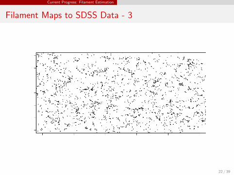
Filament Maps to SDSS Data - 3
22 / 39

Current Progress: Filament Estimation
Filament Maps to SDSS Data - 3
22 / 39

Current Progress: Uncertainty Measures
Outline
Introduction to Filaments
Filament Estimation
Uncertainty Measures
Future Work
23 / 39

Current Progress: Uncertainty Measures
The Need for Uncertainty Measure
To evaluate the quality of estimation.
To perform statistical inference.
24 / 39
Current Progress: Uncertainty Measures
Uncertianty Measures
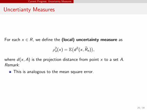
For each x ∈ R, we define the (local) uncertainty measure as
ρ2n(x) = E
(d2(x , R̂n)
),
where d(x ,A) is the projection distance from point x to a set A.Remark:
This is analogous to the mean square error.
25 / 39
Current Progress: Uncertainty Measures
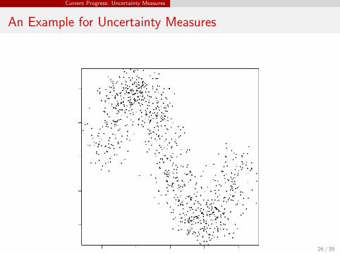
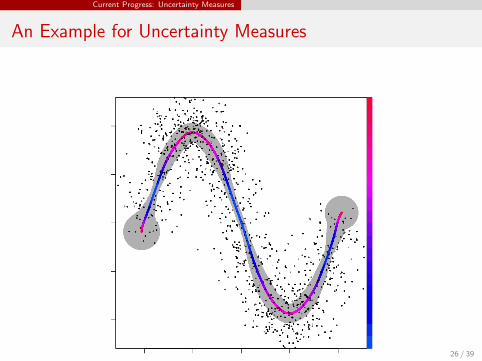
An Example for Uncertainty Measures
26 / 39

Current Progress: Uncertainty Measures
An Example for Uncertainty Measures
26 / 39
Current Progress: Uncertainty Measures
An Example for Uncertainty Measures
26 / 39
Current Progress: Uncertainty Measures
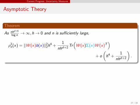
Asymptotic Theory
Theorem
As nhd+6
log n →∞, h→ 0 and n is sufficiently large,
ρ2n(x) = ‖W (x)b(x)‖2
2h4 +1
nhd+2Tr(
W (x)Σ(x)W (x)T)
+ o
(h4 +
1
nhd+2
).
b(x) ∝ ∇2(∇p(x)
): the bias, curvature of ridges.
Σ(x) ∝ p(x): the variance.
W (x) : relates to H−1(x), the significance of ridges, curvature ofdensity in subspace.
27 / 39

Current Progress: Uncertainty Measures
An Example for Uncertainty Measures
28 / 39

Current Progress: Uncertainty Measures
An Example for Uncertainty Measures
28 / 39

Current Progress: Uncertainty Measures
Estimating Uncertainty Measures
Problem: Unknown quantities.
Solution: The bootstrap.
29 / 39

Current Progress: Uncertainty Measures
Smooth Bootstrap
The smooth bootstrap is a modification of bootstrapping.Sampling from p̂n.
30 / 39

Current Progress: Uncertainty Measures
Bootstrap Uncertainty Measure
Xn = {X1, · · · ,Xn}: the original sample.
{X ∗1 , · · · ,X ∗
n }: the smooth bootstrap sample.
p̂∗n : the bootstrap KDE.
The bootstrap ridge:R̂∗n = Ridge(p̂∗
n).
The bootstrap (estimated) uncertainty measure:
ρ̂2n(x |Xn) = E
(d(x , R̂∗
n)2|Xn
), x ∈ R̂n.
31 / 39

Current Progress: Uncertainty Measures
Bootstrap Uncertainty Measure
A plug-in estimate:
ρ2n(x) = E
(d2(x , R̂n)
), x ∈ R
ρ̂2n(x |Xn) = E
(d2(x , R̂∗
n)|Xn
), x ∈ R̂n.
ρ2n(x) and ρ̂2
n(x |Xn) defined on different supports.
32 / 39

Current Progress: Uncertainty Measures
Bootstrap Consistency
Theorem
As nhd+6
log n →∞, h→ 0 and n is sufficiently large, for each x ∈ R we can
find y ∈ R̂n such that
nhd+2∣∣∣ρ̂2
n(y |Xn)− ρ2n(x)
∣∣∣ = O(h4) + OP
( log n
nhd+6
).
33 / 39

Current Progress: Uncertainty Measures
Illustration for Bootstrap Consistency
RR̂n
34 / 39

Current Progress: Uncertainty Measures
Illustration for Bootstrap Consistency
RR̂n
34 / 39

Current Progress: Uncertainty Measures
Illustration for Bootstrap Consistency
RR̂n
34 / 39

Current Progress: Uncertainty Measures
Illustration for Bootstrap Consistency
RR̂n
34 / 39

Current Progress: Uncertainty Measures
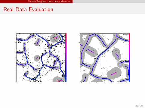
Real Data Evaluation
35 / 39

Current Progress: Uncertainty Measures
Real Data Evaluation
35 / 39
Current Progress: Uncertainty Measures
Real Data Evaluation
35 / 39
Current Progress: Uncertainty Measures
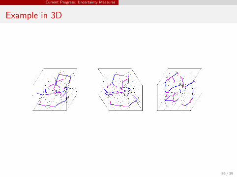
Example in 3D
36 / 39

Current Progress: Uncertainty Measures
Example in 3D
36 / 39

Future work
Outline
Introduction to Filaments
Filament Estimation
Uncertainty Measures
Future Work
37 / 39

Future work
Future Work
Confidence sets
Study of biasSolution manifoldsMore applications in astronomy
38 / 39

Future work
Future Work
Confidence setsStudy of bias
Solution manifoldsMore applications in astronomy
38 / 39

Future work
Future Work
Confidence setsStudy of biasSolution manifolds
More applications in astronomy
38 / 39

Future work
Future Work
Confidence setsStudy of biasSolution manifolds
More applications in astronomy
38 / 39

Future work
Future Work
Confidence setsStudy of biasSolution manifoldsMore applications in astronomy
38 / 39

Future work
Thank you!
39 / 39

Future work
reference
1. Asymptotic theory for density ridges. (2014) Y.-C. Chen, C. R. Genovese, L. Wasserman. (working paper)
2. Statistical analysis for cosmic filaments. (2014) Y.-C. Chen, S. Ho, P. Freeman, C. R. Genovese, Larry Wasserman.(working paper)
3. Solution manifolds in statistics. (2014) Y.-C. Chen, C. R. Genovese, L. Wasserman. (manuscript)
4. Properties of ridges and cores for two-dimensional images. (1999) J. Damon. Journal of Mathematical Imaging andVision.
5. Ridges in Image and Data Analysis. (1996) D. Eberly. Springer.
6. Nonparametric ridge estimation. (2012) C. R. Genovese, M. Perone-Pacifico, I. Verdinelli, and L. Wasserman.(arXiv:1212.5156)
7. Ridge Finding from Noisy Data. (1991) P. Hall, W. Qian and D. M. Titterington. Journal of Comp. and Graphical Stat.
8. Locally defined principal curves and surfaces. (2011) U. Ozertem and D. Erdogmus. Journal of Machine Learning
Research.
40 / 39
Future work
Density ridges
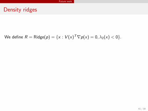
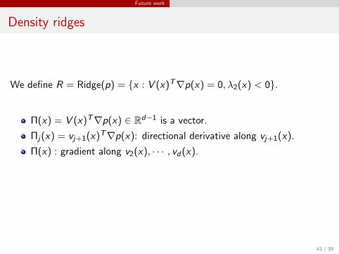
We define R = Ridge(p) = {x : V (x)T∇p(x) = 0, λ2(x) < 0}.
Π(x) = V (x)T∇p(x) ∈ Rd−1 is a vector.
Πj(x) = vj+1(x)T∇p(x): directional derivative along vj+1(x).
Π(x) : gradient along v2(x), · · · , vd(x).
Π(x) = 0: critical point in column space of V (x).
41 / 39

Future work
Density ridges
We define R = Ridge(p) = {x : V (x)T∇p(x) = 0, λ2(x) < 0}.
Π(x) = V (x)T∇p(x) ∈ Rd−1 is a vector.
Πj(x) = vj+1(x)T∇p(x): directional derivative along vj+1(x).
Π(x) : gradient along v2(x), · · · , vd(x).
Π(x) = 0: critical point in column space of V (x).
41 / 39

Future work
Density ridges
We define R = Ridge(p) = {x : V (x)T∇p(x) = 0, λ2(x) < 0}.
Π(x) = V (x)T∇p(x) ∈ Rd−1 is a vector.
Πj(x) = vj+1(x)T∇p(x): directional derivative along vj+1(x).
Π(x) : gradient along v2(x), · · · , vd(x).
Π(x) = 0: critical point in column space of V (x).
41 / 39
Future work
Density ridges
We define R = Ridge(p) = {x : V (x)T∇p(x) = 0, λ2(x) < 0}.
Π(x) = V (x)T∇p(x) ∈ Rd−1 is a vector.
Πj(x) = vj+1(x)T∇p(x): directional derivative along vj+1(x).
Π(x) : gradient along v2(x), · · · , vd(x).
Π(x) = 0: critical point in column space of V (x).
41 / 39

Future work
Density ridges
We define R = Ridge(p) = {x : V (x)T∇p(x) = 0, λ2(x) < 0}.
Π(x) = V (x)T∇p(x) ∈ Rd−1 is a vector.
Πj(x) = vj+1(x)T∇p(x): directional derivative along vj+1(x).
Π(x) : gradient along v2(x), · · · , vd(x).
Π(x) = 0: critical point in column space of V (x).
41 / 39

Future work
Geometric Interpretation
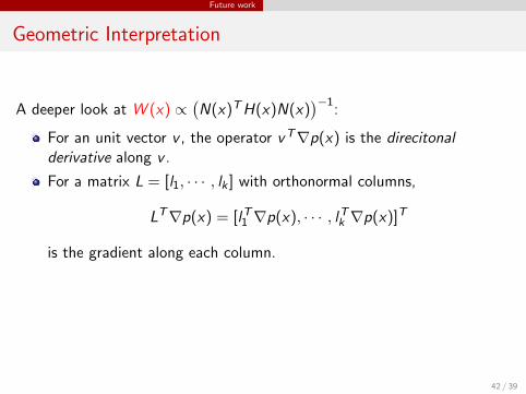
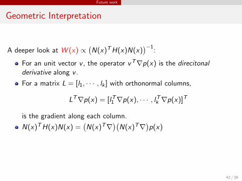
A deeper look at W (x) ∝(N(x)TH(x)N(x)
)−1:
For an unit vector v , the operator vT∇p(x) is the direcitonalderivative along v .
For a matrix L = [l1, · · · , lk ] with orthonormal columns,
LT∇p(x) = [lT1 ∇p(x), · · · , lTk ∇p(x)]T
is the gradient along each column.
N(x)TH(x)N(x) =(N(x)T∇
)(N(x)T∇
)p(x)
is the Hessian matrix constraint in column space of N(x).
42 / 39

Future work
Geometric Interpretation
A deeper look at W (x) ∝(N(x)TH(x)N(x)
)−1:
For an unit vector v , the operator vT∇p(x) is the direcitonalderivative along v .
For a matrix L = [l1, · · · , lk ] with orthonormal columns,
LT∇p(x) = [lT1 ∇p(x), · · · , lTk ∇p(x)]T
is the gradient along each column.
N(x)TH(x)N(x) =(N(x)T∇
)(N(x)T∇
)p(x)
is the Hessian matrix constraint in column space of N(x).
42 / 39

Future work
Illustration
R
43 / 39

Future work
Illustration
R
x
43 / 39

Future work
Illustration
R
x
43 / 39

Future work
Illustration
R
x
N(x)
43 / 39

Future work
Comparison of bootstrap
The bootstrap. The smooth bootstrap.
44 / 39