GREEN'S FUNCTIONS OF FILAMENT SOURCES EMBEDDED IN STRATIFIED DIELECTRIC MEDIA

Progress In Electromagnetics Research, PIER 62, 21–40, 2006

GREEN’S FUNCTIONS OF FILAMENT SOURCESEMBEDDED IN STRATIFIED DIELECTRIC MEDIA

E. A. Soliman †

IMECKapeldreef 75, B-3001 Leuven, Belgium

G. A. E. Vandenbosch

K. U. Leuven, ESAT/TELEMIC, Kasteelpark Arenberge 10B-3001 Leuven, Belgium

Abstract—In this paper a new technique for the evaluation of theGreen’s functions of filament sources in layered media, is presented.The technique is based on the annihilation of the asymptotic andsingular behaviors of a spectral Green’s function. The remainingfunction, after annihilation, is treated using a two levels discretecomplex image method (DCIM). The application of the proposedtechnique, provides a complete analytical expression for the spatialGreen’s function, in terms of the iterative value of the propagationconstant. This expression consists of the annihilating functions anda number of complex images. In order to validate the proposedtechnique, microstrip lines and slotlines are analyzed and the obtainedresults are found to agree very well with those obtained using acommercial software.

1. INTRODUCTION

Green’s functions are a very important concept in electromagnetics.They are analogous to the impulse response in systems and automaticcontrol theory. Green’s functions are the solution of the problemexcited with a hypothetical unit source. Mathematically speaking,Green’s functions provide the required electromagnetic fields due to ageneral shape source through a convolution integral. The evaluation† Also with K. U. Leuven, ESAT/TELEMIC, Kasteelpark Arenberge 10, B-3001 Leuven,Belgium

22 Soliman and Vandenbosch

procedure of the Green’s functions always starts in the spectral domain.In this domain, several recursive techniques can be employed tocalculate the required Green’s functions [1–5].

Green’s functions are the kernel of the integral equationformulation. Formulating the integral equation in the spatial domain,requires the calculation of the Green’s functions in that domain. Thespatial domain Green’s function is obtained from its spectral equivalentusing the inverse Fourier transform operator. Unfortunately, thisinverse Fourier transformation results in an integral of the Sommerfeldtype [6] whose integrand is a highly oscillatory and slowly decayingfunction. Consequently, the numerical evaluation of the Sommerfeldintegral is very time consuming. Recently, considerable interest hasbeen given to the efficient calculation of the Sommerfeld integrals. Aspectral domain Green’s function shows an asymptotic behavior at highspectral values. As a first step towards an efficient evaluation of theSommerfeld integral, this asymptotic behavior should be removed fromthe spectral Green’s function. Most of the techniques presented in theliterature are approximating this asymptotic behavior using analyticalfunctions whose inverse Fourier transform are known analytically. Theapproximating functions are subtracted from the spectral Green’sfunction and their inverses are added analytically in the spatial domain[2, 4, 5, 7].

In addition, the spectral Green’s function shows singular behaviordue to the existence of poles and branch points located along the realaxis. The physical interpretation of a pole is a surface wave mode,which can be considered as an eigen solution to the unloaded dielectriclayer structure. The behavior of the poles can also be analyticallyapproximated, subtracted from the spectral functions and their inversecounterparts are analytically added in the spatial domain [2, 4, 5, 7].

The remaining singular behavior is due to the branch points whichare associated with the existence of half-spaces in the layer structureunder investigation. Most of the techniques presented in the literatureavoid these branch points by deforming the Sommerfeld integrationpath from the real axis to another path in which the branch pointsingularities do not appear [4, 7]. Since the fast variation in the spectralGreen’s functions are essentially dominating at large spatial values, thetechnique presented in [2] provides more accurate Green’s functions athigh spatial values. In this technique, the branch point singularity isalso analytically approximated and subtracted in the spectral domain.Using Fourier transform identities, the inverse Fourier transform isobtained analytically and added. The remaining spectral functionalong the real axis is a smooth and fast decaying function, which canbe integrated numerically [2] over a finite interval.

Progress In Electromagnetics Research, PIER 62, 2006 23

Alternatively, the remaining spectral function can be integratedmore efficiently using the Discrete Complex Image Method, DCIM. Theidea of the DCIM was initiated in [8], and developed numerically in[4, 7, 9–11]. It is based on approximating the spectral Green’s functionusing short series of exponentials. This can be achieved by uniformlysampling the spectral function and applying the Generalized PencilOf Function (GPOF) technique [12], on the samples. The resultingexponentials can be analytically inverse Fourier transformed, usingappropriate identities, which results in another series in the spatialdomain. A two level DCIM approach is introduced in [13], and usedin [14]. It overcomes the difficulties associated with the conventionalDCIM approach in selecting the efficient sampling parameters. DCIMcan be applied by sampling the remaining spectral function on amodified path if the branch point singularities have not been subtracted[4, 7, 14], or along the real axis if these singularities are subtracted. Thelatter approach is adopted, for the first time, in this paper.

Section 2 presents the problem under investigation. Theevaluation of the Green’s functions in the spectral domain is presentedin Section 3. In Section 4, the techniques used to transform the Green’sfunctions to the spatial domain are presented. The implementation ofthe proposed technique is validated by analyzing microstrip lines andslotlines in Section 5. The conclusions are given in Section 6.

2. THE PHYSICAL STRUCTURE

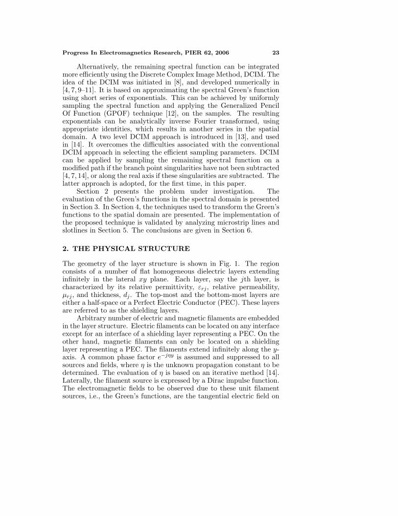
The geometry of the layer structure is shown in Fig. 1. The regionconsists of a number of flat homogeneous dielectric layers extendinginfinitely in the lateral xy plane. Each layer, say the jth layer, ischaracterized by its relative permittivity, εrj , relative permeability,µrj , and thickness, dj . The top-most and the bottom-most layers areeither a half-space or a Perfect Electric Conductor (PEC). These layersare referred to as the shielding layers.

Arbitrary number of electric and magnetic filaments are embeddedin the layer structure. Electric filaments can be located on any interfaceexcept for an interface of a shielding layer representing a PEC. On theother hand, magnetic filaments can only be located on a shieldinglayer representing a PEC. The filaments extend infinitely along the y-axis. A common phase factor e−jηy is assumed and suppressed to allsources and fields, where η is the unknown propagation constant to bedetermined. The evaluation of η is based on an iterative method [14].Laterally, the filament source is expressed by a Dirac impulse function.The electromagnetic fields to be observed due to these unit filamentsources, i.e., the Green’s functions, are the tangential electric field on


Figure 1. Geometry of a stratified dielectric media carrying filamentsources.

the interfaces carrying electric filaments and the tangential magneticfield on the interfaces carrying magnetic filaments. Time harmonicfields with time dependent factor of e−jωt, where ω is the radialfrequency, are assumed and the time factor is suppressed throughout.

3. SPECTRAL DOMAIN GREEN’S FUNCTIONS

In the spectral domain, Maxwell’s equations are transformed to thewell-known transmission line equations. In these equations, thedependency along the axis of stratification is expressed in terms of twowaves propagating in opposite directions and multiplied by unknownexpansion coefficients. These coefficients are carrying the dependencyalong the remaining axes. They can be obtained using the recursivetechnique presented in [1] and used in [2]. The details of this technique


can be found in [1] and [2], only the main equations are stated inthis section. In [1], the authors select e+

ix, e+iy, e−ix, and e−iy as the

independent field coefficients in the ith layer. In this paper, thecoefficients e+

iz, h+iz, e−iz, and h−

iz are going to be used, which are moreconvenient in the decomposition of the field into TE-to-z and TM-to-zsystems. For the TE system, the coefficients e+

iz and e−iz are vanish,and the field components in the ith layer can be written as follows:

hTEiz = h+,TE

iz

(e−γiz + ΓTE

i eγiz)

(1)

eTEix =

ηωµi

β2h+,TE

iz

(e−γiz + ΓTE

i eγiz)

(2)

eTEiy =

ξωµi

β2h+,TE

iz

(e−γiz + ΓTE

i eγiz)

(3)

hTEix =

jξγi

β2h+,TE

iz

(e−γiz − ΓTE

i eγiz)

(4)

hTEiy =

jηγi

β2h+,TE

iz

(e−γiz − ΓTE

i eγiz)

(5)

where ξ is the spectral counterpart of the spatial variable x, β =√ξ2 + η2, and γi =

√β2 − ω2µiεi is the propagation constant in the

ith layer along the direction of stratification. ΓTEi = h−,TE

iz /h+,TEiz

is defined as the reflection coefficient in the ith layer for the TEsystem. It is clear from Equations (1)–(5), that all field componentsof the TE system can be expressed in terms of h+,TE

iz and ΓTEi only.

These coefficients can be obtained by applying the recursive techniquepresented in [1] and shown in Fig. 2. Starting from ΓTE

i = 0, inthe top-most layer, and moving inward while applying the continuityconditions of the tangential fields on the source free interfaces until thejth interface, results in the calculation of all ΓTE

i , where i < j, andthe jth interface is the interface carrying the source filament. Similarlystarting from ΓTE

n = ∞, in the bottom-most layer, and moving inward,results in the calculation of all ΓTE

i , where i > j. This recurrencesequence is referred to as the inward recurrence, as shown in Fig. 2.At the jth interface, solving the two equations expressing the fielddiscontinuity, results in the evaluation of h+,TE

jz and h+,TE(j+1)z. Using

these two coefficients and applying an outward recurrence sequence, seeFig. 2, towards the top-most and the bottom-most layers, respectively,results in the evaluation of h+,TE

iz for all the layers.Similarly, for the TM system, h+

iz = h−iz = 0 and the field

components can be written as follows:

eTMiz = e+,TM

iz

(e−γiz − ΓTM

i eγiz)

(6)


Figure 2. Inward and outward recurrence techniques.


eTMix =

jξγi

β2e+,TMiz

(e−γiz + ΓTM

i eγiz)

(7)

eTMiy =

jηγi

β2e+,TMiz

(e−γiz + ΓTM

i eγiz)

(8)

hTMix =

ηωεi

β2e+,TMiz

(e−γiz − ΓTM

i eγiz)

(9)

hTMiy = −ξωεi

β2e+,TMiz

(e−γiz − ΓTM

i eγiz)

(10)

where ΓTMi = −e−,TM

iz /e+,TMiz is the reflection coefficient in the ith

layer for the TM system. Applying the inward and the outwardrecurrence sequences, as for the TE case, the coefficients e+,TM

iz andΓTM

i can be calculated for all the layers. The total lateral fields areobtained by recombining the TE and the TM systems [1]:

eix = ge,ekij ke

jx − jξge,eqij

(−jξke

jx − jηkejy

)

−ge,mkij km

jy − jξge,mqij

(−jηkm

jx + jξkmjy

)(11)

eiy = ge,ekij ke

jy − jηge,eqij

(−jξke

jx − jηkejy

)

+ge,mkij km

jx − jηge,mqij

(−jηkm

jx + jξkmjy

)(12)

hix = −gh,ekij ke

jy − jξgh,eqij

(−jηke

jx + jξkejy

)

+gh,mkij km

jx − jξgh,mqij

(−jξkm

jx − jηkmjy

)(13)

hiy = gh,ekij ke

jx − jηgh,eqij

(−jηke

jx + jξkejy

)

+gh,mkij km

jy − jηgh,mqij

(−jξkm

jx − jηkmjy

)(14)

where kejx and ke

jy are the x- and y-component of the electric filamentcurrent source located at the jth interface, while km

jx and kmjy are the

magnetic current components. Practically, the jth interface can carryeither electric or magnetic filaments. However, it is assumed that bothkinds of sources are present in order to mathematically treat bothcases simultaneously. The function gij is the spectral domain Green’sfunction representing a field observed on the ith interface due to aunit filament source located on the jth interface. The superscript ofany spectral Green’s function in Equations (11)–(14) consists of threeletters. The first letter indicates the type of field to be observed, efor electric and m for magnetic field. The second and third lettersare related to the source. The second letter indicates the type of thecurrent, e for electric and m for magnetic. The third letter is set to k


if the current source is directly used, while it is set to q if the chargederived from the current source is used.

It is worth mentioning here that all Green’s functions in Equations(11)–(14) are depending on β, and independent on ξ separately. Thefield components in the spatial domain can be obtained by performinginverse Fourier transform operations on Equations (11)–(14). Theresulting spatial domain field components are related to the spatialcurrent components and spatial Green’s functions through convolutionintegrals. It is our objective in the following section to evaluate thespatial equivalent of the spectral Green’s functions obtained in thissection.

4. SPATIAL DOMAIN GREEN’S FUNCTIONS

After evaluating the spectral Green’s functions, an inverse Fouriertransform is performed in order to transform them to the spatialdomain. Making use of the fact that the spectral Green’s functions aredependent on β, and independent on ξ separately, the inverse Fouriertransform can be written as follows:

FT−1(g(ξ)) = G(x) =1π

∞∫0

g

(√ξ2 + η2

)cos(ξx)dξ (15)

where G and g are the spatial and spectral domain Green’s functions,respectively. FT−1 is the inverse Fourier transform operator. Theintegral in (15) is a typical Sommerfeld cosine integral, which isquite time consuming to be evaluated numerically owing to its highlyoscillating and slowly decaying integrands. Several authors have giventheir interest towards the efficient evaluation of Sommerfeld integrals.The technique presented here is a combination between an extendedversion from the technique in [2] and a modified version of the techniquepresented in [14]. Consequently, it is highly recommended to consultthese works.

4.1. Annihilation of the Asymptotic and Singular Behaviors

The technique presented in [2], is based on subtracting a numberof analytical, annihilating, functions from a spectral domain Green’sfunction. These functions are representing the asymptotic and thesingular behaviors of the function. The asymptotic functions areapproximating the Green’s function at high spectral values. Thesingular functions are approximating the Green’s function around apole or a branch point. The annihilating functions are selected such


Table 1. Fourier transform pairs for the annihilating functions.

category Spectral Domain spatial Domatin

Asymptotes e−β∆ ∆η

π√

x2 + ∆2K1 η

√x2 + ∆2

1 − e−βt

βe−β∆ 1

π

[K0 η

√x2 + ∆2 − K0 η

√x2 + (t + ∆)2

]

Brach points√

β2 − K2 − β +K2

2√

β2 + K2

√η2 − K2

πxK1

√η2 − K2x −

η

πxK1(ηx) +

K2

2πK0

√η2 + K2x

Branch points1√

β2 − K2− P

β2 − K2− K0

√η2 − K2x − P

2√

η2 − K2

e−√

η2−K2x−

close to poles1√

β2 + K2− P

β2 + K2

1

πK0

√η2 + K2x +

P

2√

η2 + K2

e−√

η2+K2x

Poles1

β2 − P 2− 1

β2 + P 2

1

2√

η2 − P 2

e−√

η2−P2x − 1

2√

η2 + P 2

e−√

η2+P2x

(

(

(

(

( )

)

))

)

)

(( )

1

π

that their inverse Fourier transforms are known analytically. In [2], thespatial counterparts of the annihilating functions are given for the caseof dipole sources. For the filament source problem under investigation,the same annihilating functions are used in the spectral domain, whiletheir spatial counterparts are different due to the fact that differentinverse Fourier transform operator is used.

Table 1 lists the spectral and the spatial pairs of each annihilatingfunction. In this table, ∆ is the z-separation between the source andthe observation point, t = 1/κm and κm = κ0

√εr,m is the maximum

propagation constant in the layer structure, κ0 = ω√

µ0ε0 is thefree-space propagation constant, and εr,m is the maximum relativepermittivity in the layer structure. P and K are the spectral points,along the real axis of β, representing a pole and a branch point,respectively. Kn is the modified Bessel function of the second kindand of the nth order. In Table 1, the terms used to annihilate theasymptotes are those representing the direct term between the sourceand the observer. For most of the layer structures, these terms are thedominant terms. However, for layer structures containing very thinfilm, like in the multichip module-deposition (MCM-D) technology [14],the indirect terms resulting from the multiple reflections may becomesignificant. Consequently, for these special cases, the annihilation ofthe direct terms only, leave the function with residual asymptotes.These residual asymptotes are treated numerically in this paper viathe application of a two level discrete complex image method, DCIM.

In order to demonstrate the annihilation procedure, an electricfilament located on top of an alumina substrate, with εr = 9.9


Figure 3. Electric filament source on top of an alumina substratebacked by a PEC.

and thickness of 500 µm, backed by a PEC plane is considered, seeFig. 3. The integral equation formulation of this problem, requiresthe evaluation of two Green’s functions, namely ge,ek

11 and ge,eq11 which

correspond to the electric field observed on the air-dielectric interfacedue to the current and charge, respectively, of the electric filamentsource located on the same interface. As a representative example,only ge,eq

11 will be treated, it will be referred to as g throughout. Theother function can be treated in a similar way. Fig. 4 shows thefunction g versus β/κ0, calculated at frequency f = 5 GHz. The figureclearly shows both the asymptotic and the singular behaviors of theGreen’s function. Subtracting the annihilating functions listed in thesecond column of Table 1, results in the modified Green’s function, gmo,which is plotted in Fig. 5. It is clear that the modified function is freefrom any asymptotic or singular behaviors. It is suitable to be treatednumerically along the real axis of β using DCIM.

4.2. Discrete Complex Image Method (DCIM)

In [2], the modified function is inverted numerically over a finiteinterval. In this paper, the two level discrete complex image method,DCIM, introduced in [13] is applied on the modified function. Unlike[14], the application of the DCIM technique is carried out along thereal axis of β, in both the first and second levels. This selection is aconsequence of the complete annihilation of the singularities along thereal axis.

The first and second levels are defined in the spectrum β2 → β1

and κ0 → β2, respectively, where κ0 is the free-space propagationconstant. The values of β1 and β2 are not strictly specified. Numericalinvestigations on several layer structures, have shown that β1 = 100 κ0

is enough to extract any residual asymptotic behavior of the spectralGreen’s function in the first level. β2 is selected such that it is higher


0 5 10 15 20 25 30 35 40-3E-4

-2E-4

-1E-4

0E+0

1E-4

2E-4

3E-4

4E-4

0

g

Real

Im ag

0 1 2 3 4 5-3E-4

-2E-4

-1E-4

0E+0

1E-4

2E-4

3E-4

4E-4

/

Figure 4. Spectral charge Green’s function for the electric filamentsource of Fig. 3, f = 5 GHz.

0 5 10 15 20 25 30 35 40-3E-4

-2E-4

-1E-4

0E+0

1E-4

2E-4

3E-4

4E-4

0

RealImag

0 1 2 3 4 5-1E-3

-8E-4

-6E-4

-4E-4

-2E-4

0E+0

2E-4

g mo

/β κ

Figure 5. Modified spectral charge Green’s function after subtractingthe annihilating functions.


than κm, where κm is the maximum total propagation constant in thelayer structure under investigation. This selection is based on the factthat any residual singular behavior, which could not be annihilatedperfectly, should be located in the spectrum below κm. The functionin the first level is sampled with low sampling rate, while in the secondlevel, higher sampling rate is required to pick-up the relatively fastervariation of the function.

The parametric equation of the first level, according to which thesamples are taken, can be written as follows:

β = β2 + (β1 − β2)t, t : 0 → 1 (16)

Using GPOF [12], the spectral domain Green’s function in the firstlevel can be written as follows:

g1 =N1∑i=1

a1ieα1it

N1∑i=1

a1ieα1i(β−β2)/(β1−β2) (17)

where g1 is the spectral Green’s function in the first level, N1 is thenumber of exponentials required to approximate the function in thefirst level, a1i and α1i are the complex residue and exponent of theith exponential term, respectively. The approximated function, g1,matches the original function in the first level, β : β2 → β1, wherethe function shows an asymptotic behavior. Although the Green’sfunction asymptote associated with the direct term has been removed,the investigation of the function in the first level is performed in orderto extract the asymptote associated with the indirect terms appearingin thin film layer structures. The extrapolation of the function g1 in thesecond level does not match the original function, g. Another DCIMprocedure should be applied in the second level to approximate thedifference between the original function, g, and the extrapolation of g1

[13]. The parametric equation of the second level is:

β = κ0 + (β2 − κ0)t, t : 0 → 1 (18)

Applying GPOF on the difference: g2 = g − g1, allows one to write:

g2 =N2∑i=1

a2ieα2it =

N2∑i=1

a2ieα2i(β−κ0)/(β2−κ0) (19)

where N2 is the number of exponentials required to approximate thedifference function in the second level, a2i and α2i are the complexresidue and exponent of the ith exponential term, respectively. Beingthe difference between the original and the approximated function


0 5 10 15 20 25 30 35 40-1E-3

-8E-4

-6E-4

-4E-4

-2E-4

0E+0

2E-4

4E-4

0

g mo

2nd level 1st level

Real (exact)Imag (exact)

Real (DCIM)Imag (DCIM)

β/κ

Figure 6. Exact and DCIM approximation of the modified spectralcharge Green’s function.

in the first level, the extrapolation of the approximated function,g2, should vanish in the first level. Hence, over all the investigatedspectrum, β : κ0 → β1, the modified spectral Green’s function can beapproximated as follows:

gmo(β) = g1 + g2 =N1∑i=1

a1ieα1i(β−β2)/(β1−β2) +

N2∑i=1

a2ieα2i(β−κ0)/(β2−κ0)

(20)The exact and the two levels DCIM approximation of the modifiedcharge function gmo, of the example in Fig. 3, are plotted in Fig. 6.The figure shows very good approximation for the modified functionin both the first and second levels. Using a Fourier transform identity[15], the modified spectral Green’s function in Equation (20) can bewritten in the spatial domain as follows:

Gmo(x) =η

π(β1 − β2)

N1∑i=1

±α1iα1i

ρ1iK1(ηρ1i)e

α1iβ2β1−β2

η

π(β2 − κ0)

N2∑i=1

±α2iα2i

ρ2iK1(ηρ2i)e

α2iκ0β2−κ0 (21)

where ρ1i =√

(α1i/(β1 − β2))2 + x2 and ρ2i =√

(α2i/(β2 − κ0))2 + x2.


0 0.01 0.02 0.03 0.04 0.05 0.06 0.07 0.08 0.09 0.1-5.0

-4.5

-4.0

-3.5

-3.0

-2.5

-2.0

-1.5

-1.0

-0.5

0.0

x 0

| golG

| 01

om

1.792.59

0

0

0

==

=

/

ηηη

κκκ

λ

Figure 7. Modified spatial charge Green’s function.

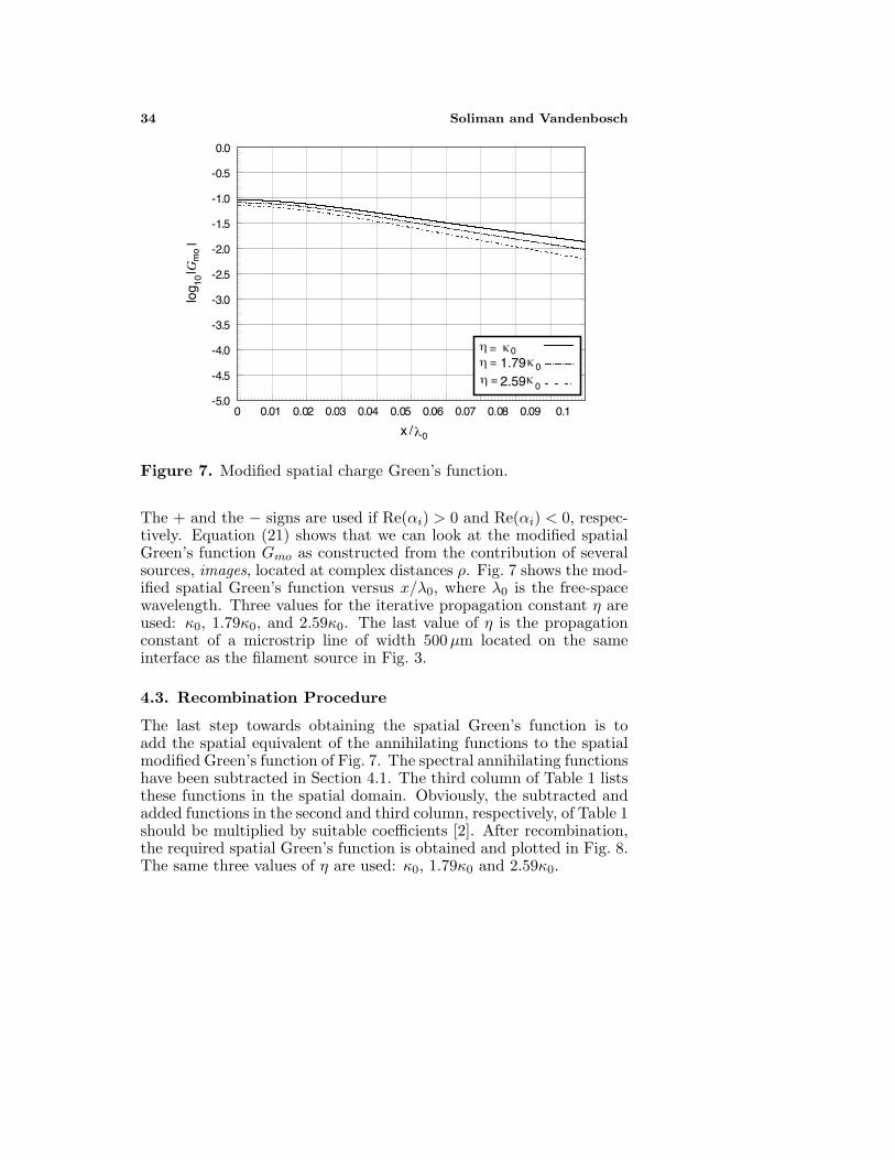
The + and the − signs are used if Re(αi) > 0 and Re(αi) < 0, respec-tively. Equation (21) shows that we can look at the modified spatialGreen’s function Gmo as constructed from the contribution of severalsources, images, located at complex distances ρ. Fig. 7 shows the mod-ified spatial Green’s function versus x/λ0, where λ0 is the free-spacewavelength. Three values for the iterative propagation constant η areused: κ0, 1.79κ0, and 2.59κ0. The last value of η is the propagationconstant of a microstrip line of width 500µm located on the sameinterface as the filament source in Fig. 3.

4.3. Recombination Procedure

The last step towards obtaining the spatial Green’s function is toadd the spatial equivalent of the annihilating functions to the spatialmodified Green’s function of Fig. 7. The spectral annihilating functionshave been subtracted in Section 4.1. The third column of Table 1 liststhese functions in the spatial domain. Obviously, the subtracted andadded functions in the second and third column, respectively, of Table 1should be multiplied by suitable coefficients [2]. After recombination,the required spatial Green’s function is obtained and plotted in Fig. 8.The same three values of η are used: κ0, 1.79κ0 and 2.59κ0.


0 0.01 0.02 0.03 0.04 0.05 0.06 0.07 0.08 0.09 0.1-5.0

-4.5

-4.0

-3.5

-3.0

-2.5

-2.0

-1.5

-1.0

-0.5

0.0

x 0

| golG

|01

1.792.59

0

0

0

==

=

/

ηηη

κκκ

λ

Figure 8. Spatial charge Green’s function.

5. VALIDATION RESULTS

In this section, two types of planar guiding structures are analyzed,namely: microstrip lines and slotlines. The analysis of these guidingstructures is carried out using a method of moment (MoM) formulationsimilar to that presented in [14]. The core of this MoM uses the spatialdomain Green’s functions calculated via the proposed approach in thispaper. The analysis of the structures under investigation is carried outusing Agilent-Momentum [16] as well. Comparison between ours andMomentum’s results is performed.

5.1. Microstrip Lines

The microstrip line studied in this sub-section is built on an Aluminasubstrate with dielectric constant of εr = 9.9, and thickness of 500µm.The substrate is backed by a perfect electric conductor (PEC) plate.On top of the substrate a thin film of BenzoCycloButene (BCB)is deposited. The dielectric constant of this layer is 2.7, and itsthickness is d. Above the BCB film, a microstrip line made of copper(σ = 58 × 106 1/Ωm) with width of 500µm and thickness of 2µm, isplaced. Another thin film of BCB with thickness of 10µm, is placedon top of the microstrip line. The deposition of the BCB thin films isa typical feature of the MCM-D technology [14]. These films are used


5 7.5 10 12.5 15 17.5 20 22.5 25 27.5 304.0

4.5

5.0

5.5

6.0

6.5

7.0

7.5

8.0

Frequency (GHz)

d = 0 m

d = 10 m

d = 20 m

500

10dBCB

BCB 5002

Alumina, = 9.9r

r, e

ffMomentumOurs

µ

µ

ε

ε

µ

Figure 9. Effective dielectric constant versus frequency for themicrostrip line using 3 uniform segments along the width (alldimensions are in µm).

to isolate the layers of interconnects of the MCM.The effective dielectric constant versus frequency obtained using

both our solver and Momentum is plotted in Fig. 9. The cross sectionof the microstrip line is also shown in Fig. 9. Three uniform segmentsare used to model the width of the microstrip line. The thicknessof the bottom BCB film takes the values: 0, 10 µm, and 20 µm.Very good agreement between our results and those of Momentum isobserved. This agreement validates indirectly the proposed techniquefor calculating the spatial domain Green’s functions.

It is clear from the figure that as the thickness of the bottomBCB film increases, the effective dielectric constant of the microstripline decreases. This means that the phase velocity increases and thepropagation delay decreases. Consequently, we can conclude thatmicrostrip lines in the MCM-D technology are performing better thanthose fabricated with the conventional technology. The thickness ofthe top BCB film is found to have a negligible effect on the effectivedielectric constant of the microstrip line. This comes from the factthe most of the power is concentrated in the high dielectric constantsubstrate below the microstrip line. Hence, the thickness of the topBCB film is held constant at 10 µm.


5 7.5 10 12.5 15 17.5 20 22.5 25 27.5 302.0

2.4

2.8

3.2

3.6

4.0

4.4

4.8

5.2

Frequency (GHz)

d = 0 m

d = 10 m

d = 20 m

500

10dBCB

BCB 50

Alumina, = 9.9r

r, e

ffMomentumOurs

µ

µ

µ

ε

ε

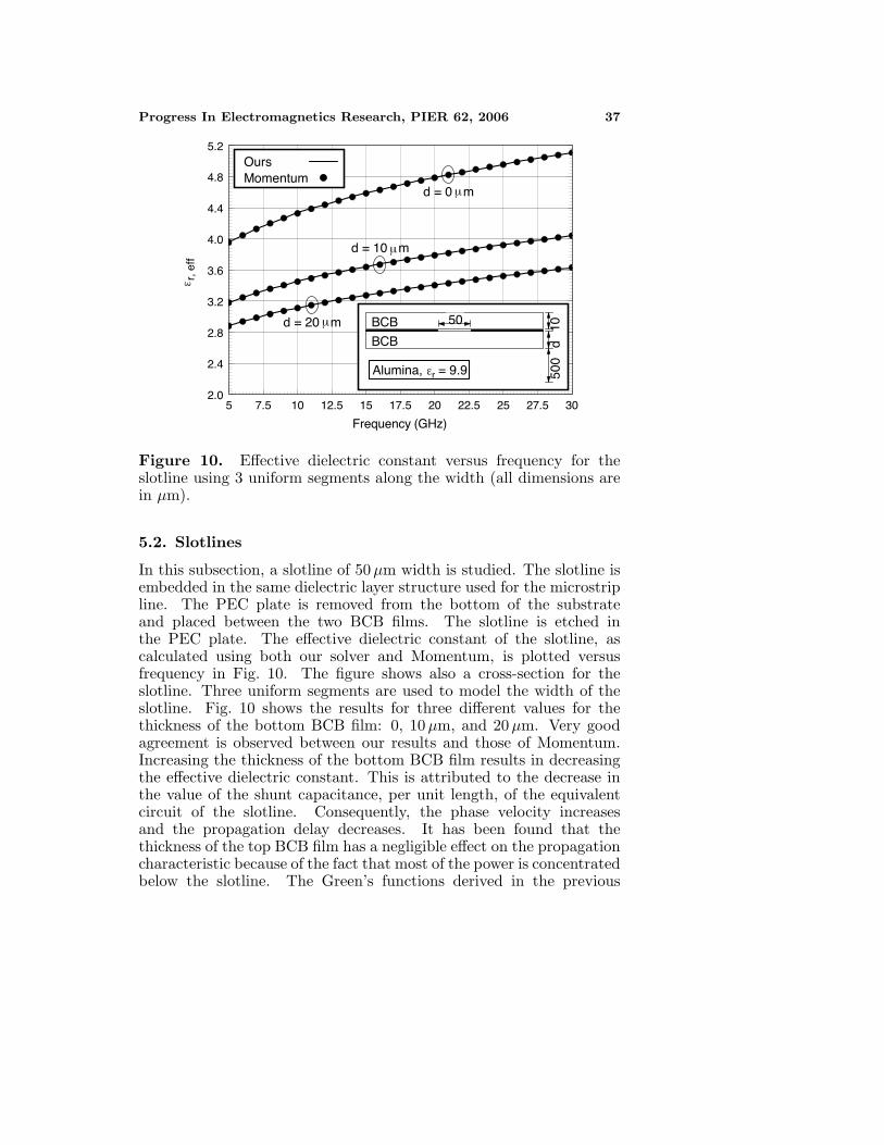
Figure 10. Effective dielectric constant versus frequency for theslotline using 3 uniform segments along the width (all dimensions arein µm).

5.2. Slotlines

In this subsection, a slotline of 50 µm width is studied. The slotline isembedded in the same dielectric layer structure used for the microstripline. The PEC plate is removed from the bottom of the substrateand placed between the two BCB films. The slotline is etched inthe PEC plate. The effective dielectric constant of the slotline, ascalculated using both our solver and Momentum, is plotted versusfrequency in Fig. 10. The figure shows also a cross-section for theslotline. Three uniform segments are used to model the width of theslotline. Fig. 10 shows the results for three different values for thethickness of the bottom BCB film: 0, 10 µm, and 20 µm. Very goodagreement is observed between our results and those of Momentum.Increasing the thickness of the bottom BCB film results in decreasingthe effective dielectric constant. This is attributed to the decrease inthe value of the shunt capacitance, per unit length, of the equivalentcircuit of the slotline. Consequently, the phase velocity increasesand the propagation delay decreases. It has been found that thethickness of the top BCB film has a negligible effect on the propagationcharacteristic because of the fact that most of the power is concentratedbelow the slotline. The Green’s functions derived in the previous


sections are used in the calculation of the propagation characteristicof the slotline. Consequently, the agreement between our solver andMomentum validates the theory and the implementation of the Green’sfunctions.

6. CONCLUSIONS

In this paper, a modified technique for the evaluation of theGreen’s functions of filament sources in layered media is presented.It generalizes the technique in [2] to be suitable for applicationscontaining wire-like sources. Moreover, it also generalizes the two levelsDCIM technique presented in [13] to the problem under investigation.This generalized two levels DCIM is used to replace the conventionalnumerical integral used in [2] for inverting the modified spectralGreen’s function. The mixture of the two generalized techniquesallows complete analytical representation for spatial Green’s functionsof filament sources embedded in layer structure containing thin films.

Since the solution procedure of the planar guiding structureproblems is iterative and requiring the evaluation of a new set ofspatial Green’s functions at each iteration. The technique presentedin this paper is found to be numerically efficient. This comes fromthe fact that after the first iteration, the spectral Green’s functionsare expressed as number of analytical functions: the annihilatingfunctions, and number of complex images. Consequently, the spatialdomain Green’s functions are also expressed analytically as a functionof the iterative value of the propagation constant. Then for the nextiterations, the new set of spatial Green’s functions is obtained bysimple substitution in the analytical expressions with a new value ofthe iterative variable.

The technique presented in this paper provides higher accuracythan that presented in [14], specially at large spatial distances. This isa consequence of the careful treatment of the singular behaviors whosecontributions are known to dominate at these distances. The accuracyof proposed technique is validated by analyzing a number of microstriplines and slotlines. Our results are compared with those obtained usinga commercial software. Very good agreement is observed.

REFERENCES

1. Vandenbosch, G. A. E. and A. R. Van de Capelle, “Mixed-potential integral expression formulation of the electric field in astratified dielectric medium — Application to the case of a probe


current source,” IEEE Trans. Antennas Propagat., Vol. 40, 806–817, 1992.

2. Demuynck, F. J., G. A. E. Vandenbosch, andA. R. Van de Capelle, “The expansion wave concept —Part I: Efficient calculation of the spatial Green’s functions in astratified dielectric medium,” IEEE Trans. Antennas Propagat.,Vol. 46, 397–406, 1998.

3. Michalski, K. A. and D. Zheng, “Electromagnetic scattering andradiation by surfaces of arbitrary shape in layered media, PartI: Theory,” IEEE Trans. Antennas Propagat., Vol. 38, 335–344,1990.

4. Dural, G. and M. I. Aksun, “Closed-form Green’s function forgeneral sources and stratified media,” IEEE Trans. MicrowaveTheory Tech., Vol. 43, 1545–1552, 1995.

5. Hsu, C.-I. G., R. F. Harrington, K. A. Michaliski, and D. Zheng,“Analysis of multiconductor transmission lines of arbitrary crosssection in multilayered uniaxial media,” IEEE Trans. MicrowaveTheory Tech., Vol. 41, 70–78, 1993.

6. Sommerfeld, A., Partial Differential Equations in Physics,Academic, New York, 1949.

7. Chow, Y. L., J. J. Yang, D. G. Fang, and G. E. Howard, “A closed-form spatial Green’s function for the thick microstrip substrate,”IEEE Trans. Microwave Theory Tech., Vol. 39, 588–592, 1991.

8. Mohsen, A., “On the evaluation of Sommerfeld integrals,” IEEProc. Pt. H., Vol. 129, 177–182, 1982.

9. Mahmoud, S. F. and A. Mohsen, “Assessment of image theory forfield evaluation over a multi-layer earth,” IEEE Trans. AntennasPropagat., Vol. 33, 1054–1058, 1985.

10. Yang, J. J., Y. L. Chow, and D. G. Fang, “Discrete compleximages of a three-dimensional dipole above and within a lossyground,” IEE Proc. Pt. H., Vol. 138, 319–326, 1991.

11. Chow, Y. L., J. J. Yang, and G. E. Howard, “Complex imagesfor electrostatic field computation in multilayered media,” IEEETrans. Microwave Theory Tech., Vol. 39, 1120–1125, 1991.

12. Hua, Y. and T. K. Sarker, “Generalized pencil-of-function methodfor extracting poles of an EM system from its transient response,”IEEE Trans. Antennas Propagat., Vol. 37, 229–234, 1989.

13. Aksun, M. I., “A robust approach for the derivation of closed-form Green’s functions,” IEEE Trans. Microwave Theory Tech.,Vol. 44, 651–658, 1996.

14. Soliman, E. A., P. Pieters, E. Beyne, and G. A. E. Vandenbosch,


“Numerically efficient spatial domain moment method formultislot transmission lines in layered media — Application tomultislot lines in MCM-D technology,” IEEE Trans. MicrowaveTheory Tech., Vol. 47, 1782–1787, 1999.

15. Gradshteyn, I. S. and I. M. Ryzhik, Table of Integrals, Series andProducts, Academic Press, 1980.

16. Momentum, version 4.8, Agilent Technologies, 2003.

GREEN'S FUNCTIONS OF FILAMENT SOURCES EMBEDDED IN STRATIFIED DIELECTRIC MEDIA

Documents

Transcript of GREEN'S FUNCTIONS OF FILAMENT SOURCES EMBEDDED IN STRATIFIED DIELECTRIC MEDIA