Uncertainty Measures and Limiting Distributions forFilament Estimation

Yen-Chi ChenCarnegie Mellon University

5000 Forbes Ave.Pittsburgh, PA 15213, USA

yenchic@andrew.cmu.edu

Christopher R. GenoveseCarnegie Mellon University

5000 Forbes Ave.Pittsburgh, PA 15213, USA

genovese@stat.cmu.edu

Larry WassermanCarnegie Mellon University

5000 Forbes Ave.Pittsburgh, PA 15213, USA

larry@stat.cmu.edu

ABSTRACTA filament is a high density, connected region in a pointcloud. There are several methods for estimating filamentsbut these methods do not provide any measure of uncer-tainty. We give a definition for the uncertainty of estimatedfilaments and we study statistical properties of the estimatedfilaments. We show how to estimate the uncertainty mea-sures and we construct confidence sets based on a bootstrap-ping technique. We apply our methods to astronomy dataand earthquake data.

Categories and Subject DescriptorsG.3 [PROBABILITY AND STATISTICS]: Multivari-ate statistics, Nonparametric statistics

General TermsTheory

Keywordsfilaments, ridges, density estimation, manifold learning

1. INTRODUCTIONA filament is a one-dimensional, smooth, connected struc-ture embedded in a multi-dimensional space. Filamentsarise in many applications. For example, matter in theuniverse tends to concentrate near filaments that comprisewhat is known as the cosmic-web [Bond et al. 1996], andthe structure of that web can serve as a tracer for estimat-ing fundamental cosmological constants. Other examplesinclude neurofilaments and blood-vessel networks in neu-roscience [Lalonde and Strazielle 2003], fault lines in seis-mology [USGS 2003], and landmark paths in computer vi-sion [Hile et al. 2009].

Consider point-cloud data X1, X2, . . . , Xn in Rd, drawn in-dependently from a density p with compact support. Wedefine the filaments of the data distribution as the ridgesof the probability density function p. (See Section 2.1 for

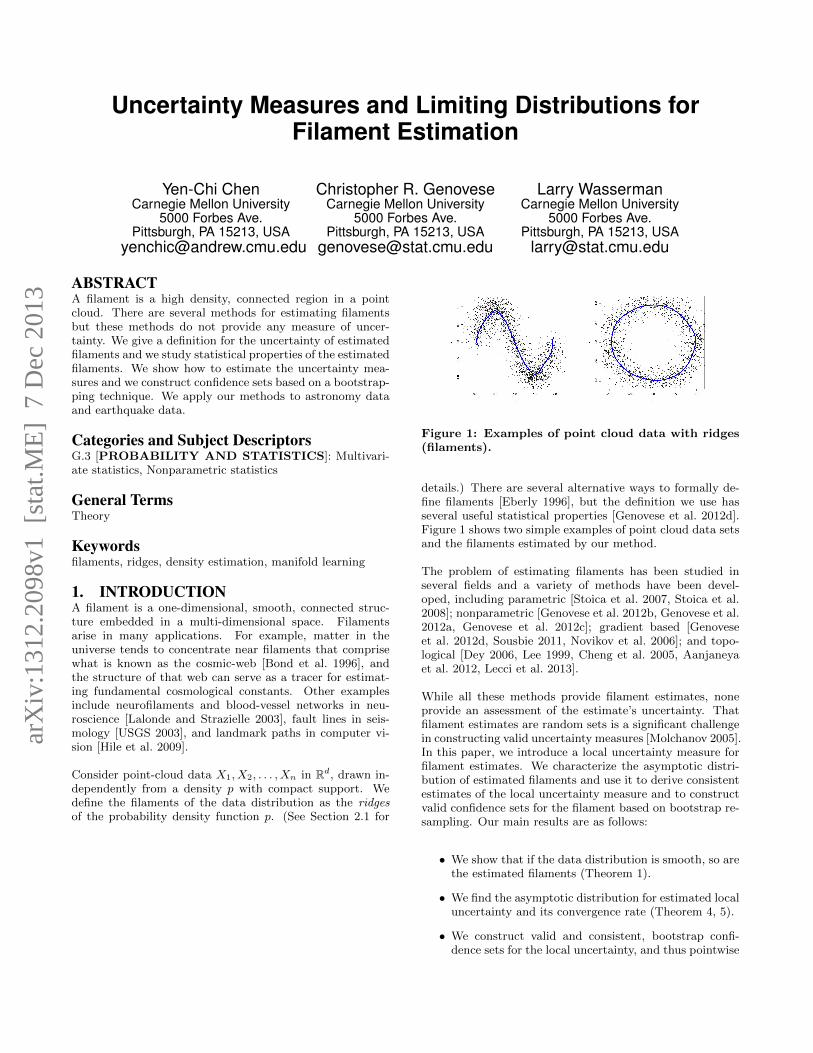
Figure 1: Examples of point cloud data with ridges(filaments).

details.) There are several alternative ways to formally de-fine filaments [Eberly 1996], but the definition we use hasseveral useful statistical properties [Genovese et al. 2012d].Figure 1 shows two simple examples of point cloud data setsand the filaments estimated by our method.

The problem of estimating filaments has been studied inseveral fields and a variety of methods have been devel-oped, including parametric [Stoica et al. 2007, Stoica et al.2008]; nonparametric [Genovese et al. 2012b, Genovese et al.2012a, Genovese et al. 2012c]; gradient based [Genoveseet al. 2012d, Sousbie 2011, Novikov et al. 2006]; and topo-logical [Dey 2006, Lee 1999, Cheng et al. 2005, Aanjaneyaet al. 2012, Lecci et al. 2013].

While all these methods provide filament estimates, noneprovide an assessment of the estimate’s uncertainty. Thatfilament estimates are random sets is a significant challengein constructing valid uncertainty measures [Molchanov 2005].In this paper, we introduce a local uncertainty measure forfilament estimates. We characterize the asymptotic distri-bution of estimated filaments and use it to derive consistentestimates of the local uncertainty measure and to constructvalid confidence sets for the filament based on bootstrap re-sampling. Our main results are as follows:

• We show that if the data distribution is smooth, so arethe estimated filaments (Theorem 1).

• We find the asymptotic distribution for estimated localuncertainty and its convergence rate (Theorem 4, 5).

• We construct valid and consistent, bootstrap confi-dence sets for the local uncertainty, and thus pointwise

arX

iv:1

312.

2098

v1 [

stat

.ME

] 7

Dec

201

3

confidence sets for the filament (Theorem 6).

We apply our methods to point cloud data from examples inAstronomy and Seismology and demonstrate that they yielduseful confidence sets.

2. BACKGROUND2.1 Density RidgesLet X1, · · ·Xn be random sample from a distribution withcompact support in Rd that has density p. Let g(x) = ∇p(x)and H(x) denote the gradient and Hessian, respectively,of p(x). We begin by defining the ridges of p, as definedin [Genovese et al. 2012d, Ozertem and Erdogmus 2011,Eberly 1996]. While there are many possible definitions ofridges, this definition gives stability in the underlying den-sity, estimability at a good rate of convergence, and fastreconstruction algorithms, as described in [Genovese et al.2012d]. In the rest of this paper, the filaments to be esti-mated are just the one-dimensional ridges of p.

A mode of the density p – where the gradient g is zero andall the eigenvalues of H are negative – can be viewed asa zero-dimensional ridge. Ridges of dimension 0 < s < dgeneralize this to the zeros of a projected gradient where thed − s smallest eigenvalues of H are negative. In particularfor s = 1,

R ≡ Ridge(p) = x : G(x) = 0, λ2(x) < 0, (1)

where

G(x) = V (x)V (x)T g(x) (2)

is the projected gradient. Here, the matrix V is defined asV (x) = [v2(x), · · · vd(x)] for eigenvectors v1(x), v2(x), ..., vd(x)of H(x) corresponding to eigenvalues λ1(x) ≥ λ2(x) ≥ · · · ≥λd(x) Because one-dimensional ridges are the primary con-cern of this paper, we will refer to R in (1) as the “ridges”of p.

Intuitively, at points on the ridge, the gradient is the sameas the largest eigenvector and the density curves downwardsharply in directions orthogonal to that. When p is smoothand the eigengap β(x) = λ1(x)−λ2(x) is positive, the ridgeshave the all essential properties of filaments. That is, Rdecomposes into a set of smooth curve-like structures withhigh density and connectivity. R can also be characterizedthrough Morse theory [Guest 2001] as the collection of (d−1)-critical-points along with the local maxima, also knownas the set of 1-ascending manifolds with their local-maximalimit points [Sousbie 2011].

2.2 Ridge EstimationWe estimate the ridge in three steps: density estimation,thresholding, and ascent. First, we estimate p from fromthe data X1, . . . , Xn. Here, we use the well-known kerneldensity estimator (KDE) defined by

pn(x) =1

nhd

n∑i=1

K

(||x−Xi||

h

), (3)

where the kernel K is a smooth, symmetric density functionsuch as a Gaussian and h ≡ hn > 0 is the bandwidth whichcontrols the smoothness of the estimator. Because ridge

estimation can tolerate a fair degree of oversmoothing (asshown in [Genovese et al. 2012d]), we select h by a simplerule that tends to oversmooth somewhat, the multivariateSilverman’s rule [Silverman 1986]. Under weak conditions,

this estimator is consistent; specifically, ||pn − p||∞P→ 0 as

n → ∞. (We say that Xn converges in probability to b,

written XnP→ b if, for every ε > 0, P (|Xn − b| > ε) → 0 as

n→∞.)

Second, we threshold the estimated density to eliminate low-probability regions and the spurious ridges produced in pnby random fluctuations. Here, we remove points with esti-mated density less than τ ||pn||∞ for a user-chosen threshold0 < τ < 1.

Finally, for a set of points above the density threshold, wefollow the ascent lines of the projected gradient to the ridge,which is the the subspace constrainted mean shift (SCMS)algorithm [Ozertem and Erdogmus 2011]. This procedurecan be viewed as estimating the ridge by applying the Ridgeoperator to pn:

Rn = Ridge(pn). (4)

Note that Rn is a random set.

2.3 Bootstrapping and Smooth BootstrappingThe bootstrap [Efron 1979] is a statistical method for as-sessing the variability of an estimator. Let X1, . . . , Xn be arandom sample from a distribution P and let θ(P ) be somefunctional of P to be estimated, such as the mean of the dis-tribution or (in our case) the ridge set of its density. Given

some procedure θ(X1, . . . , Xn) for estimating θ(P ) we es-

timate the variability of θ by resampling from the originaldata.

Specifically, we draw a bootstrap sample X∗1 , . . . , X∗n inde-

pendently and with replacement from the set of observed

data points X1, . . . , Xn and compute the estimate θ∗ =

θ(X∗1 , . . . , X∗n) using the bootstrap sample as if it were the

data set.

This process is repeated B times, yielding B bootstrap sam-

ples and corresponding estimates θ∗1 , . . . , θ∗B . The variability

in these estimates is then used to assess the variability in the

original estimate θ ≡ θ(X1, . . . , Xn). For instance, if θ is a

scalar, the variance of θ is estimated by

1

B

B∑b=1

(θ∗b − θ)2

where θ = 1B

∑Bb=1 θ

∗b . Under suitable conditions, it can be

shown that this bootstrap variance estimates – and confi-dence sets produced from it – are consistent.

The smooth bootstrap is a variant of the bootstrap that canbe useful in function estimation problems where the sameprocedure is used except the bootstrap sample is drawn fromthe estimated density p instead of the original data. We useboth variants below.

3. METHODS

We measure the local uncertainty in a filament (ridge) esti-

mator Rn by the expected distance between a specified pointin the original filament R and the estimated filament:

ρ2n(x) =

Epd2(x, Rn) if x ∈ R0 otherwise

, (5)

where d(x,A) is the distance function:

d(x,A) = infy∈A|x− y|. (6)

The local uncertainty measure can be understood as theexpected dispersion for a given point in the original filamentto the estimated filament based on sample with size n. Thetheoretical analysis of ρ2n(x) is given in theorem 5.

3.1 Estimating Local UncertaintyBecause ρ2n(x) is defined in terms unknown distribution pand the unknown filament set R, it must be estimated. Weuse bootstrap resampling to do this, defining an estimateof local uncertainty on the estimated filaments. For each

of B bootstrap samples, X∗(b)1 , · · · , X∗(b)n , we compute the

kernel density estimator p∗(b)n , the ridge estimate R

∗(b)n =

Ridge(p∗(b)n ), and the divergence ρ2(b)(x) = d2(x, R

∗(b)n ) for

all x ∈ Rn. We estimate ρ2n(x) by

ρ2n(x) =1

B

B∑b=1

ρ2(b)(x) ≡ E(d2(x, R∗n)|X1, · · · , Xn), (7)

for each x ∈ Rn, where the expectation is from the (known)bootstrap distribution. Algorithm 1 provides pseudo-codefor this procedure, and Theorem 6 shows that the estimateis consistent under smooth bootstrapping.

Algorithm 1 Local Uncertainty Estimator

Input: Data X1, . . . , Xn.1. Estimate the filament from X1, . . . , Xn; denote the

estimate by Rn.

2. Generate B bootstrap samples: X∗(b)1 , . . . , X

∗(b)n for

b = 1, . . . , B.3. For each bootstrap sample, estimate the filament, yield-

ing R∗(b)n for b = 1, . . . , B.

4. For each x ∈ Rn, calculate ρ2(b)(x) = d2(x, R∗(b)n ), b =

1, . . . , B.5. Define ρ2n(x) = meanr21(x), . . . , r2B(x).Output: ρ2n(x).

3.2 Pointwise Confidence SetsConfidence sets provide another useful assessment of uncer-tainty. A 1−α confidence set is a random set computed fromthe data that contains an unknown quantity with at leastprobability 1− α. We can construct a pointwise confidenceset for filaments from the distance function (6). For each

point x ∈ Rn, let r1−α(x) be the (1 − α) quantile value of

d(x, R∗) from the bootstrap. Then, define

C1−α(X1, · · · , Xn) =⋃x∈R

B(x, r1−α(x)). (8)

This confidence set capture the local uncertainty: for a point

x ∈ Rn with low (high) local uncertainty, the associated ra-dius r1−α(x) is small (large). But note that the confidence

set attains 1 − α coverage around each point; the coverageof the entire filament set is lower. That is, we can have highprobability to cover each point but the probability to simul-taneously cover all points (the whole filament set) might belower.

Algorithm 2 Pointwise Confidence Set

Input: Data X1, . . . , Xn; significance level α.1. Estimate the filament from X1, . . . , Xn; denote this

by Rn.

2. Generates bootstrap samples X∗(b)1 , . . . , X∗(b)n for b =

1, . . . , B.3. For each bootstrap sample, estimate the filament, call

this R∗(b)n .

4. For each x ∈ Rn, calculate ρ2(b)(x) = d2(x, R∗(b)n ), b =

1, . . . , B.5. Let r1−α(x) = Q1−α(ρ(1)(x), . . . , ρ(B)(x)).

Output:⋃x∈Rn

B(x, r1−α(x)) where B(x, r) is theclosed ball with center x and radius r.

4. THEORETICAL ANALYSISFor the filament set R, we assume that it can be decomposedinto a finite partition

R1, · · · , Rk

such that each Ri is a one dimensional manifold. Such apartition can be constructed by the equation of traversal inpage 56 of [Eberly 1996]. For each Ri, we can parametrizeit by a function φi(s) : [0, 1] → Ri from the equation oftraversal mentioned with suitable scaling.

For simplicity, in the following proofs we assume that thefilament set R is a single Ri so that we can construct theparametrization φ easily. All theorems and lemmas we provecan be applied to the whole filament set R =

⋃iRi by re-

peating the process for each individual Ri.

4.1 Smoothness of Density RidgesTo study the properties of the uncertainty estimator, wefirst need to establish some results about the smoothness ofthe filament. The following theorem provides conditions forsmoothness of the filaments. Let Ck denote the collectionof k times continuously differentiable functions.

Theorem 1 (Smoothness of Filaments). Let φ(s) :[0, 1] → R be a parameterization of filament set R, and fors0 ∈ [0, 1], let U ⊂ R be an open set containing φ(s0). Ifp is Ck and the eigengap β(x) > 0 for x ∈ U , then φ(s) isCk−2 for s ∈ φ−1(U).

Theorem 1 says that filaments from a smooth density will besmooth. Moreover, estimated filaments from the KDE willbe smooth if the kernel function is smooth. In particular, ifwe use Gaussian kernel, which is C∞, then the correspond-ing filaments will be C∞ as well.

4.2 Frenet FrameIn the arguments that follow, it is useful to have a well-defined “moving” coordinate system along a smooth curve.

R

e1(s1)e2(s1)

e2(s2)

e1(s2)e1(s3)

e2(s3)

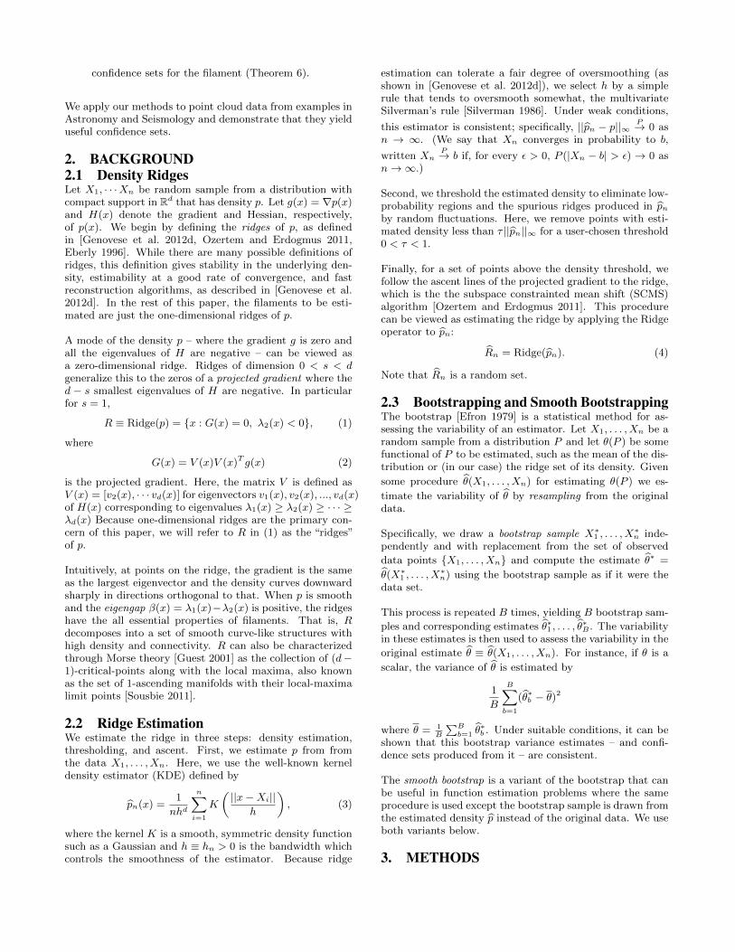
Figure 2: An example for Frenet frame in two di-mension.

Let γ : R 7→ Rd be an arc-length parametrization for a Ck+1

curve with k ≥ d. The Frenet frame [Kuhnel 2002] along γis a smooth family of orthogonal bases at γ(s)

e1(s), e2(s), · · · ed(s)

such that e1(s) = γ′(s) determines the direction of the curve.The other basis elements e2(s), · · · , ed(s) are called the cur-vature vectors and can be determined by a Gram-Schmidtconstruction.

Assume the density is Cd+3. We can construct a Frenetframe for each point on the filaments. Let e1(s), · · · , ed(s)be the Frenet frame of φ(s) such that

e1(s) =φ′(s)

|φ′(s)|

ej(s) =ej(s)

|ej(s)|

ej(s) = φ(j)(s)−j−1∑i=1

< φ(j)(s), ei(s) > ei(s), j = 2, · · · , d,

where φ(j)(s) is the jth derivative of the φ(s) and < a, b >is the inner product of vector a, b. An important fact isthat the basis element ej(s) is Cd+3−j , j = 1, 2 · · · d. Frenetframes are widely used in dynamical systems because theyprovide a unique and continuous frame to describe trajecto-ries.

4.3 Normal space and distance measureThe reach of R, denoted by κ(R), is the smallest real num-ber r such that each x ∈ y : d(y,R) ≤ r has a uniqueprojection onto R [Federer 1959].

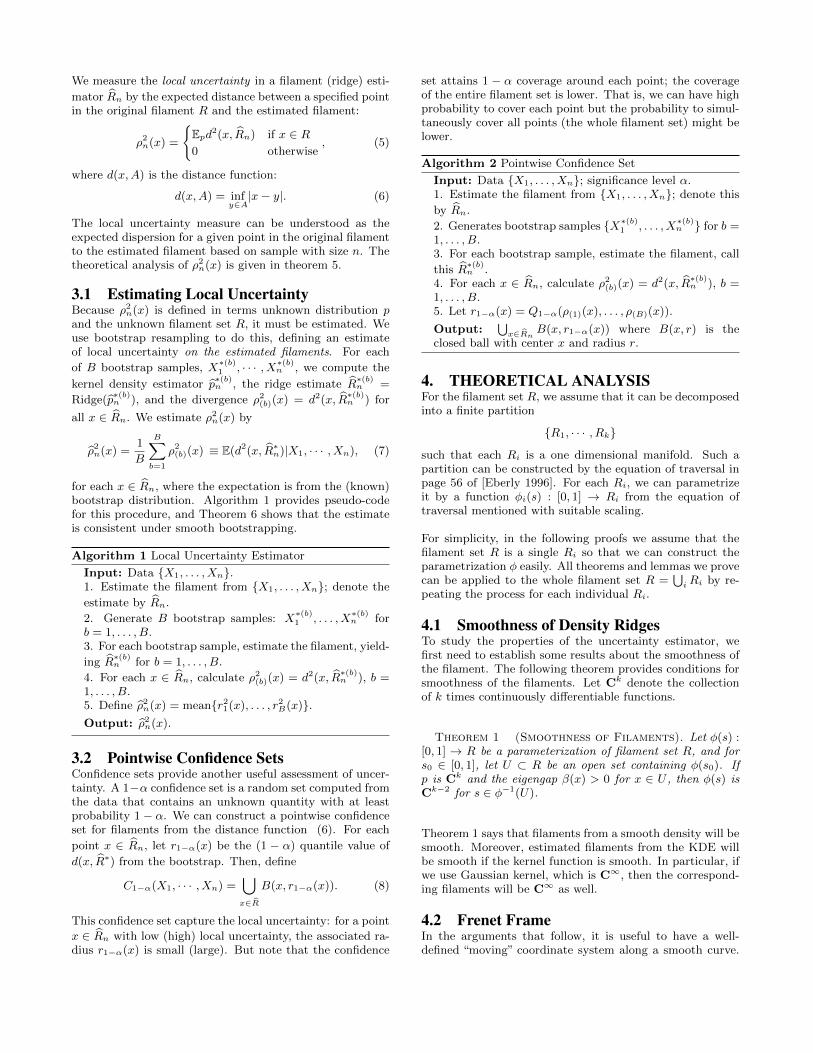
We define the normal space L(s) of φ(s) by

L(s) = d∑i=2

αiei(s) ∈ Rd : α22 + · · ·+ α2

d ≤ κ(R)2. (9)

Note that since we have second derivative of φ(s) exists andfinite, the reach will be bounded from below.

Finally, define the Hausdorff distance between two subsetsof Rd by

dH(A,B) = infε : A ⊂ B ⊕ ε and B ⊂ A⊕ ε, (10)

where A⊕ε =⋃x∈AB(x, ε) and B(x, ε) = y : ‖x−y‖ ≤ ε.

4.4 Local uncertainty

R

L(s1)

L(s2)

φ(s1)

φ(s2)

e2(s1)

e3(s1)

e2(s2)

e3(s2)

Figure 3: An example for the normal space L(s)along a ridge in three dimensional.

Let the estimated filament be the ridge of KDE. We assumethe following:

(K1) The kernel K is Cd+3.

(K2) The kernel K satisfies condition K1 in page 5 of [Gineand Guillou 2002].

(P1) The true density p is in Cd+3.

(P2) The ridges of p have positive reach.

(P3) The ridges of p are closed. For example, Figure 1-(b).

(K1) and (K2) are very mild assumptions on the kernel func-tion. For instance, Gaussain kernels satisfy both. (P1-P3)are assumptions on the true density. (P1) is a smoothnesscondition. (P2) is a smoothness assumption on the ridge.(P3) is included to avoid boundary bias when estimatingthe filament near endpoints.

Now we introduce some norms and semi-norms characteriz-ing the smoothness of the density p. A vector α = (α1, . . . , αd)of non-negative integers is called a multi-index with |α| =α1 + α2 + · · ·+ αd and corresponding derivative operator

Dα =∂α1

∂xα11

· · · ∂αd

∂xαdd

,

where Dαf is often written as f (α). For j = 0, . . . , 4, define

‖p‖(j)∞ = maxα: |α|=j

supx∈Rd

|p(α)(x)|. (11)

When j = 0, we have the infinity norm of p; for j > 0, theseare semi-norms. We also define

‖p‖∗∞,k = maxj=0,··· ,k

‖p‖(j)∞ . (12)

It is easy to verify that this is a norm. Next we recall atheorem in [Genovese et al. 2012d] which establish the link of

Hausdorff distance between R, Rn with the metric betweendensity.

Theorem 2 (Theorem 6 in [Genovese et al. 2012d]).Under conditions in [Genovese et al. 2012d], as ||p− pn||∗∞,3is sufficiently small , we have

dH(R, Rn) = OP (||p− pn||∗∞,2).

R

Rn

L(s1)

L(s2)

φ(s1)

φ(s2)

φn(s1)

φn(s2)e2(s1)

e3(s1)

e2(s2)

e3(s2)

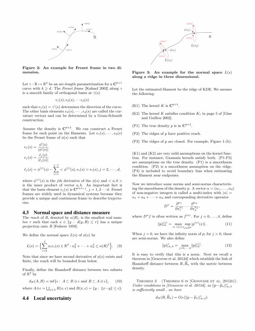
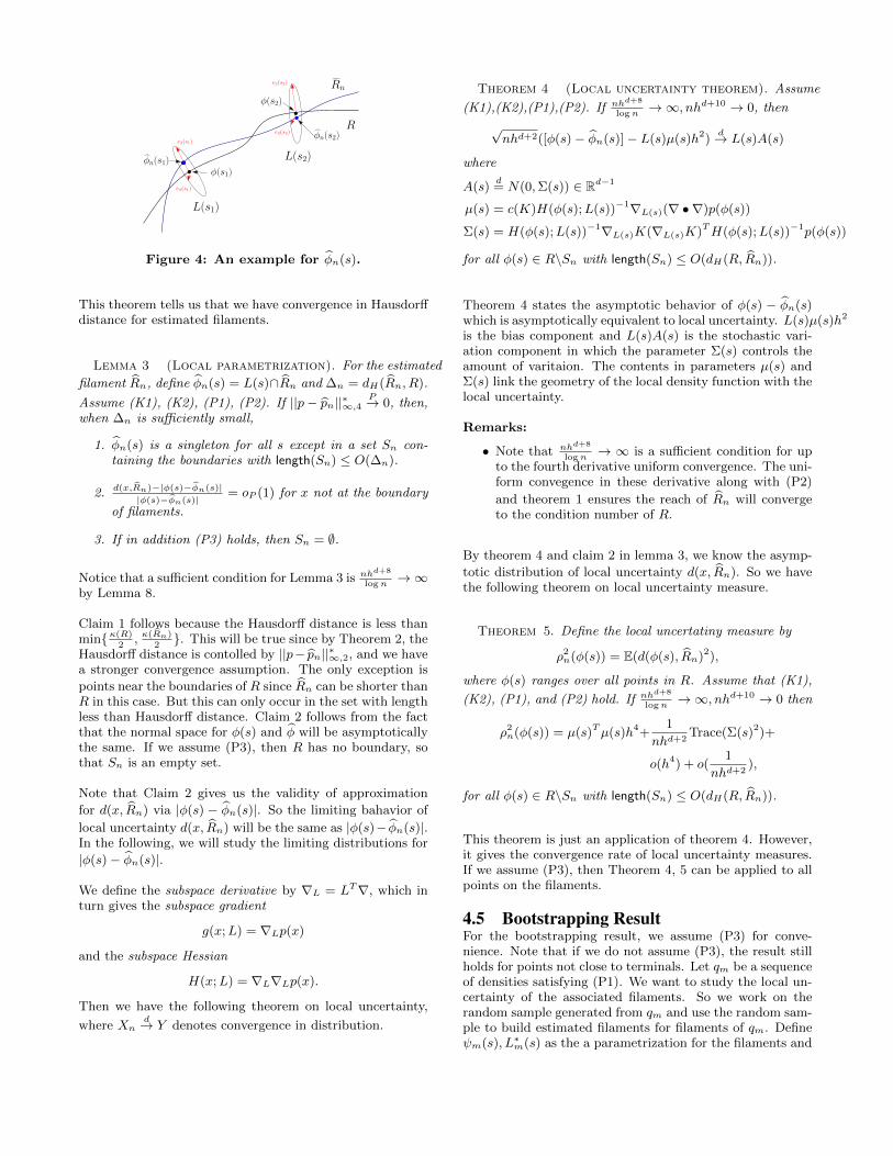
Figure 4: An example for φn(s).

This theorem tells us that we have convergence in Hausdorffdistance for estimated filaments.

Lemma 3 (Local parametrization). For the estimated

filament Rn, define φn(s) = L(s)∩Rn and ∆n = dH(Rn, R).

Assume (K1), (K2), (P1), (P2). If ||p− pn||∗∞,4P→ 0, then,

when ∆n is sufficiently small,

1. φn(s) is a singleton for all s except in a set Sn con-taining the boundaries with length(Sn) ≤ O(∆n).

2. d(x,Rn)−|φ(s)−φn(s)||φ(s)−φn(s)|

= oP (1) for x not at the boundary

of filaments.

3. If in addition (P3) holds, then Sn = ∅.

Notice that a sufficient condition for Lemma 3 is nhd+8

logn→∞

by Lemma 8.

Claim 1 follows because the Hausdorff distance is less thanminκ(R)

2, κ(Rn)

2. This will be true since by Theorem 2, the

Hausdorff distance is contolled by ||p− pn||∗∞,2, and we havea stronger convergence assumption. The only exception is

points near the boundaries of R since Rn can be shorter thanR in this case. But this can only occur in the set with lengthless than Hausdorff distance. Claim 2 follows from the factthat the normal space for φ(s) and φ will be asymptoticallythe same. If we assume (P3), then R has no boundary, sothat Sn is an empty set.

Note that Claim 2 gives us the validity of approximation

for d(x, Rn) via |φ(s) − φn(s)|. So the limiting bahavior of

local uncertainty d(x, Rn) will be the same as |φ(s)− φn(s)|.In the following, we will study the limiting distributions for

|φ(s)− φn(s)|.

We define the subspace derivative by ∇L = LT∇, which inturn gives the subspace gradient

g(x;L) = ∇Lp(x)

and the subspace Hessian

H(x;L) = ∇L∇Lp(x).

Then we have the following theorem on local uncertainty,

where Xnd→ Y denotes convergence in distribution.

Theorem 4 (Local uncertainty theorem). Assume

(K1),(K2),(P1),(P2). If nhd+8

logn→∞, nhd+10 → 0, then

√nhd+2([φ(s)− φn(s)]− L(s)µ(s)h2)

d→ L(s)A(s)

where

A(s)d= N(0,Σ(s)) ∈ Rd−1

µ(s) = c(K)H(φ(s);L(s))−1∇L(s)(∇ •∇)p(φ(s))

Σ(s) = H(φ(s);L(s))−1∇L(s)K(∇L(s)K)TH(φ(s);L(s))−1p(φ(s))

for all φ(s) ∈ R\Sn with length(Sn) ≤ O(dH(R, Rn)).

Theorem 4 states the asymptotic behavior of φ(s) − φn(s)which is asymptotically equivalent to local uncertainty. L(s)µ(s)h2

is the bias component and L(s)A(s) is the stochastic vari-ation component in which the parameter Σ(s) controls theamount of varitaion. The contents in parameters µ(s) andΣ(s) link the geometry of the local density function with thelocal uncertainty.

Remarks:

• Note that nhd+8

logn→ ∞ is a sufficient condition for up

to the fourth derivative uniform convergence. The uni-form convegence in these derivative along with (P2)

and theorem 1 ensures the reach of Rn will convergeto the condition number of R.

By theorem 4 and claim 2 in lemma 3, we know the asymp-

totic distribution of local uncertainty d(x, Rn). So we havethe following theorem on local uncertainty measure.

Theorem 5. Define the local uncertatiny measure by

ρ2n(φ(s)) = E(d(φ(s), Rn)2),

where φ(s) ranges over all points in R. Assume that (K1),

(K2), (P1), and (P2) hold. If nhd+8

logn→∞, nhd+10 → 0 then

ρ2n(φ(s)) = µ(s)Tµ(s)h4+1

nhd+2Trace(Σ(s)2)+

o(h4) + o(1

nhd+2),

for all φ(s) ∈ R\Sn with length(Sn) ≤ O(dH(R, Rn)).

This theorem is just an application of theorem 4. However,it gives the convergence rate of local uncertainty measures.If we assume (P3), then Theorem 4, 5 can be applied to allpoints on the filaments.

4.5 Bootstrapping ResultFor the bootstrapping result, we assume (P3) for conve-nience. Note that if we do not assume (P3), the result stillholds for points not close to terminals. Let qm be a sequenceof densities satisfying (P1). We want to study the local un-certainty of the associated filaments. So we work on therandom sample generated from qm and use the random sam-ple to build estimated filaments for filaments of qm. Defineψm(s), L∗m(s) as the a parametrization for the filaments and

R(p)

R(qm)

φ(s1)

φ(s2)

φψm

ψm(ξm(s1))

ψm(ξm(s2))

ξm

Figure 5: An example for ξm(s) along with φ, ψm.

associated normal space of qm. Then we have the followingconvergence theorem for a sequence of densities convergingto p.

Theorem 6. Assume that (P1–3) hold. Let qm be a se-quence of probability densities that satisfy (P1), (P2), and‖p− qm‖∗∞,3 → 0 as m→∞.

If dH(R(qm), R(p)) is sufficiently small, we can find a bijec-tion ξm : [0, 1] 7→ [0, 1] such that

1. |ψm(ξm(s))− φ(s)| → 0.

2.∣∣∣<φ′(s),ψ′

m(ξm(s))>

|ψ′m(ξm(s))||φ′(s)|

∣∣∣→ 1.

3. sups∈[0,1]

|µ(s; qm)− µ(s; p)| → 0.

4. sups∈[0,1]

|Σ(s; qm)− Σ(s; p)| → 0.

In particular, if we use pn = qn with nhd+8

logn→∞, nhd+10 →

0, then the above result holds with high probability.

Note that the local uncertainty measure has unknown sup-port and unknown parameters given in theorem 5. Claim1 shows the convergence in support while claim 3,4 provethe consistency of the parameters controlling uncertainties.This theorem states that if we have a sequence of densitiesconverging to a limiting density, then the local uncertaintywill converge in a sense.

Remarks:

• Notice that ψm(ξm(s)) need not be the same as L(s)∩R(qm). The latter one lives in the normal space of φ(s)but the former need only be a continuously bijectivemapping. The projection that maps s to the pointL(s) ∩R(qm) is one choice of ξm.

• The last result holds immediately from Lemma 8 as

we pick nhd+8

logn→ ∞, nhd+10 → 0. The bandwidth in

this case will ensure uniform convergence in probabilityup to the forth derivative which is sufficient to thecondition.

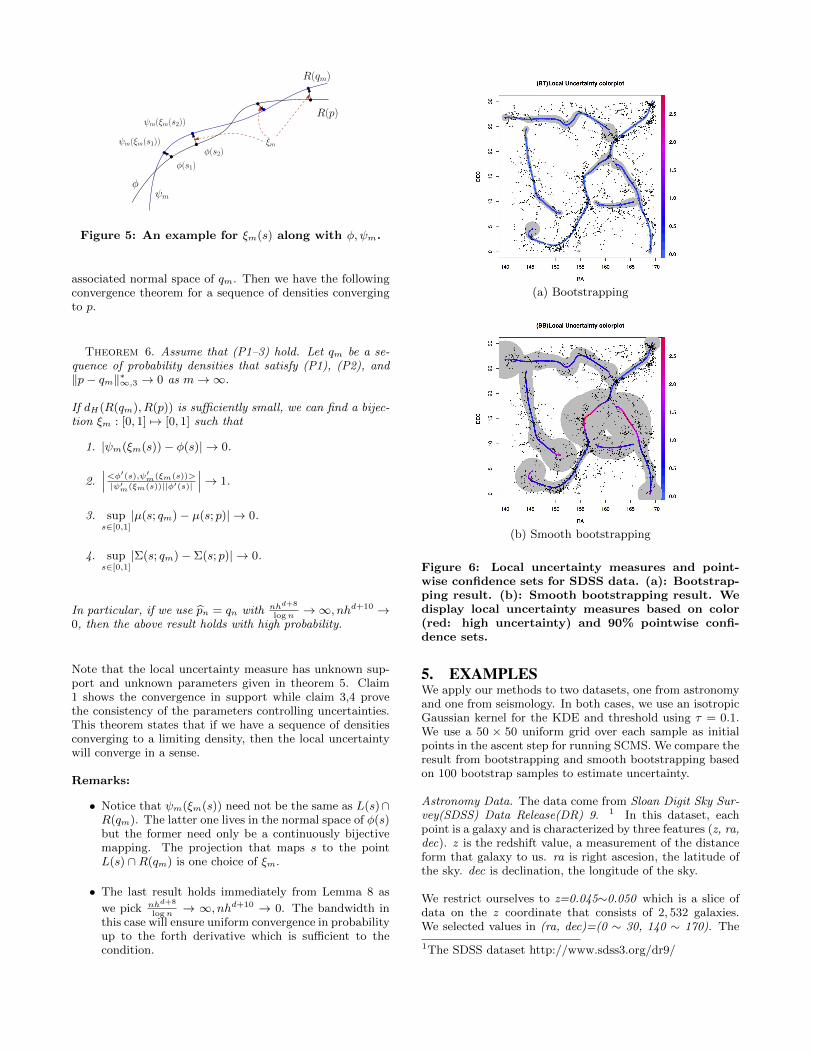
(a) Bootstrapping

(b) Smooth bootstrapping

Figure 6: Local uncertainty measures and point-wise confidence sets for SDSS data. (a): Bootstrap-ping result. (b): Smooth bootstrapping result. Wedisplay local uncertainty measures based on color(red: high uncertainty) and 90% pointwise confi-dence sets.

5. EXAMPLESWe apply our methods to two datasets, one from astronomyand one from seismology. In both cases, we use an isotropicGaussian kernel for the KDE and threshold using τ = 0.1.We use a 50 × 50 uniform grid over each sample as initialpoints in the ascent step for running SCMS. We compare theresult from bootstrapping and smooth bootstrapping basedon 100 bootstrap samples to estimate uncertainty.

Astronomy Data. The data come from Sloan Digit Sky Sur-vey(SDSS) Data Release(DR) 9. 1 In this dataset, eachpoint is a galaxy and is characterized by three features (z, ra,dec). z is the redshift value, a measurement of the distanceform that galaxy to us. ra is right ascesion, the latitude ofthe sky. dec is declination, the longitude of the sky.

We restrict ourselves to z=0.045∼0.050 which is a slice ofdata on the z coordinate that consists of 2, 532 galaxies.We selected values in (ra, dec)=(0 ∼ 30, 140 ∼ 170). The

1The SDSS dataset http://www.sdss3.org/dr9/

bandwidth h is 2.41.

Figure 6 displays the local uncertainty measures with point-wise confidence sets. The red color indicates higher lo-cal uncertainty while the blue color stands for lower uncer-tianty. Bootstrapping shows a very small local uncertaintyand very narrow pointwise confidence sets. Smooth boot-stapping yields a loose confidence sets but it shows a clearpattern of local uncertainty which can be explained by ourtheorems.

From Figure 6, we identify four cases associated with highlocal uncertainty: high curvature of the filament, flat den-sity near filaments, terminals (boundaries) of filaments, andintersecting of filaments. For the points near curved fila-ments, we can see uncertainty increases in every case. Thiscan be explained by theorem 4. The curvature is related tothe third derivative of density from the definition of ridges.From theorem 4, we know the bias in filament estimation isproportional to the third derivative. So the estimation forhighly curved filaments tends to have a systematic bias infilament estimation and our uncertainty measure capturesthis bias successfully.

For the case of a flat density, by theorem 4, we know both thebias and variance of local uncertainty is proportional to theinverse of the Hessian. A flat density has a very small Hes-sian matrix and thus the inverse will be huge; this raises theuncertainty. Though our theorem can not be applied to ter-minals of filaments, we can still explain the high uncertianty.Points near terminals suffer from boundary bias in densityestimation. This leads to an increase in the uncertainty. Forregions near connections, the eigengap β(x) = λ1(x)−λ2(x)will approach 0 which causes instability of the ridge sinceour definition of ridge requires β(x) > 0. All cases withhigh local uncertainty can be explained by our theoreticalresult. So the data analysis is consistent with our theory.

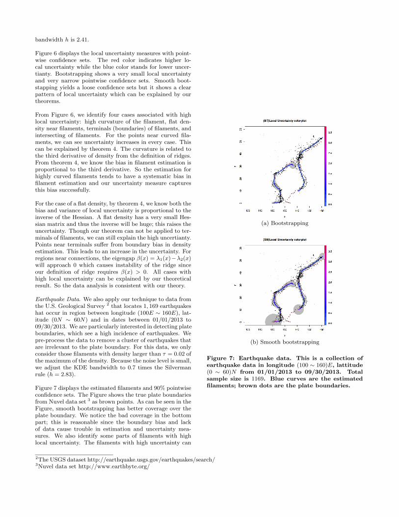
Earthquake Data. We also apply our technique to data fromthe U.S. Geological Survey 2 that locates 1, 169 earthquakeshat occur in region between longitude (100E ∼ 160E), lat-itude (0N ∼ 60N) and in dates between 01/01/2013 to09/30/2013. We are particularly interested in detecting plateboundaries, which see a high incidence of earthquakes. Wepre-process the data to remove a cluster of earthquakes thatare irrelevant to the plate boundary. For this data, we onlyconsider those filaments with density larger than τ = 0.02 ofthe maximum of the density. Because the noise level is small,we adjust the KDE bandwidth to 0.7 times the Silvermanrule (h = 2.83).

Figure 7 displays the estimated filaments and 90% pointwiseconfidence sets. The Figure shows the true plate boundariesfrom Nuvel data set 3 as brown points. As can be seen in theFigure, smooth bootstrapping has better coverage over theplate boundary. We notice the bad coverage in the bottompart; this is reasonable since the boundary bias and lackof data cause trouble in estimation and uncertainty mea-sures. We also identify some parts of filaments with highlocal uncertainty. The filaments with high uncertainty can

2The USGS dataset http://earthquake.usgs.gov/earthquakes/search/3Nuvel data set http://www.earthbyte.org/

(a) Bootstrapping

(b) Smooth bootstrapping

Figure 7: Earthquake data. This is a collection ofearthquake data in longitude (100 ∼ 160)E, lattitude(0 ∼ 60)N from 01/01/2013 to 09/30/2013. Totalsample size is 1169. Blue curves are the estimatedfilaments; brown dots are the plate boundaries.

be explained by theorem 4. The data analysis again supportour theoretical result.

In both Figure 6, 7, we see a clear picture on the uncertaintyassessment for filament estimation. In data from two orthree dimension, we can visualize uncertainties in estimationof filaments with different colors or confidence regions. Thatis, we can display estimation and the uncertainty in the sameplot.

6. DISCUSSION AND FUTURE WORKIn this paper, we define a local uncertainty measure for fila-ment estimation and study its theoretical properties. Weapply bootstrap resampling to estimate local uncertaintymeasures and construct confidence sets, and we prove thatboth are consistent and data analysis also supports our re-sult. Our method provides one way to numerically quantifythe uncertainty for estimating filaments. We also visualizeuncertatiny measures with estimated filaments in the sameplot; this can be one easy way to show estimation and theuncertainty simultaneously.

Our approach has no constraints on the dimension of thedata so it can be extended to data from higher dimension(although the confidence sets will be larger). Our defini-tion of local uncertainty and our estimation method can beapplied to other geometric estimation algorithms, which wewill investigate in the future.

APPENDIXA. PROOFS

Proof of Theorem 1. For the ridge set R, it is a collec-tion of solutions toG(x) = V (x)V (x)T∇p(x) as the eigengapβ(x) > 0. But V (x) is a d×(d−1) orthonormal basis. So thesolution to G(x) = V (x)V (x)T∇p(x) = 0 is equal to the so-lution to F (x) = V (x)T∇p(x) = 0. Now F (x) : Rd 7→ Rd−1.Hence, implicit function theorem tells us that the differen-tiablilty of a local graph (z, g(z)) : z ∈ R, g(z) ∈ Rd−1 isthe same as F (x) when β(x) > 0. Now since the local graphis parametrized by one variable, we can reparametrize it bya curve φ(x). And the differentiability of the curve is thesame as F (x).

From a slight modification from theorem 3 in [Genovese et al.2012d], the kth order derivative of F (x) depends on k+ 2thorder derivative of density if the eigengap β(x) > 0. Hence,if the density is Ck and we consider an open set U withβ(x) > 0∀x ∈ U , then we have F (x) is Ck−2 on U so theresult follows.

To prove theorem 4, we need the following lemmas:

Lemma 7. Let pn(x) be KDE for p(x). Assume our ker-nel satisfies (K1), (K2). If nhd+2 →∞, nhd+10 → 0, h→ 0.Then ∇pn(x) admits an asymptotic normal distribution by

√nhd+2(∇pn(x)−∇p(x)−B(x)h2)

d→ N(0,Σ0(x)) (13)

where

B(x) =m2(K)

2∇(∇ •∇)p(x) (14)

Σ0(x) = ∇K(∇K)T p(x) (15)

K is the kernel used and m2(K) is a constant of kernel.

Proof. For KDE pn,

pn(x) =1

n

n∑i=1

1

hdK(

x−Xih

). (16)

Hence for ∇pn,

∇pn =1

n

n∑i=1

1

hd∇K(

x−Xih

)

=1

n

n∑i=1

Φ(x;Xi).

Notice that each Φ(x;Xi) is independent and identically dis-tributed.

We will show that Φ(x;Xi) satisfies conditions for Lyapounov’scondition so that we have Central Limit Theorem (CLT) re-sult for it. WLOG, we consider the third moment and focuson partial derivative over a direction, say j, we want

(nE(|Φj(x;Xi)− E(Φj(x;Xi))|3))13

(nV ar(Φj(x;Xi)))12

→ 0 (17)

where Φj(x;Xi) = 1hd

∂∂xj

K(x−Xih

) = 1hd+1

∂K∂xj

(x−Xih

).

This is equivalent to show

n2E(|Φj(x;Xi)− E(Φj(x;Xi))|3)2

n3V ar(Φj(x;Xi))3→ 0 (18)

Now we put an upper bound on (18), then we have

n2E(|Φj(x;Xi)− E(Φj(x;Xi))|3)2

n3V ar(Φj(x;Xi))3≤ n2E(|Φj(x;Xi)|3)2

n3V ar(Φj(x;Xi))3.

We assume that∫

( ∂K∂xj

(u))2du = C2 < ∞,∫

( ∂K∂xj

(u))3du =

C3 <∞ for all j = 1, · · · , d. Therefore by Taylor expansionover density and take the first order, we have

n2E(|Φj(x;Xi)|3)2

n3V ar(Φj(x;Xi))3=n2(C3p(x)

h2d+3 + o( 1h2d+3 ))2

n3(C2p(x)

hd+2 + o( 1hd+2 ))3

= O(1

nhd)

= o(1)

As a result, Lyapounov’s condition is satisfied and this holdsfor all j = 1, · · · , d; so we have CLT for Φ(x;Xi).

By multivariate CLT we have

V ar(Φ(x;Xi))− 1

2 [∇pn − E(Φ(x;Xi))]d→ N(0, Id).

where Id is the identity matrix of dimension d.

By theorem 4 in [Chacon et al. 2011], we have

E(Φ(x;Xi)) = ∇p(x) +m2(K)

2∇(∇ •∇)p(x)h2 +O(h4)

= ∇p(x) +B(x)h2 +O(h4)

V ar(Φ(x;Xi)) =1

nhd+2∇K(∇K)T p(x) + o(

1

nhd+2)

=Σ0(x)

nhd+ o(

1

nhd)

Therefore, as nhd+2 →∞ and h→ 0,

√nhd+2Σ0(x)−

12 (∇pn(x)−∇p(x)−B(x)h2 −O(h4))

d→ N(0, Id)

Now since nhd+10 → 0 so√nhd+2O(h4) tends to 0 and

multiply Σ0(x)12 in both side, we get

√nhd+2(∇pn(x)−∇p(x)−B(x)h2)

d→ N(0,Σ0(x))

This completes the proof.

Lemma 8. ([Gine and Guillou 2002]; version of [Genoveseet al. 2012d])Assume (K1), (P1) and the kernel function satisfies condi-

tions in [Gine and Guillou 2002]. Then we have

||fn,h − f ||∞,k = O(h2) +OP (logn

nhd+2k). (19)

Lemma 9. For a density p, let R be its filaments. Forany points x on R, let the Hessian at x be H(x) with eigen-vectors [v1, · · · , vd] and eigenvalues λ1 > 0 > λ2 ≥ · · ·λd.Consider any subspace L spanned by a basis [e2, · · · ed] withe1 be the normal vector for L. Then a sufficient and neces-sary condition for x be a local mode of p constrained in Lis

d∑i=1

λi(vTi ej)

2 < 0,∀j = 2, · · · , d. (20)

A sufficient condition for (20) is

(vT1 e1)2 >λ1

λ1 − λ2. (21)

Proof. Let the Hessian of density p at x be H(x) witheigenvectors [v1, · · · , vd] and associated eigenvalues λ1 ≥λ2 ≥ · · ·λd. Consider any subspace L spanned by a basis[e2, · · · ed] with e1 be the normal vector for L

For any x on the ridge, we have λ1 > 0 > λ2. x is themode constrained in the subspace L if ∇L∇Lp(x) is negativedefinite. By spectral decomposition, we can write

∇L∇Lp(x) = LTH(x)L

= LTU(x)Ω(x)U(x)LT ,

where U(x) = [v1, · · · , vd] and Ω(x) is a diagonal matrix ofeigenvalues. So this matrix will be negative definite if andonly if all its diagonoal elements are negative.

That is, the sufficient and necessary condition is

(∇L∇Lp(x))ii < 0, i = 1, · · · , d− 1. (22)

We explicitly derive the form of (22) and consider the suffi-cient and necessary condition:

(∇L∇Lp(x))jj = (LTU(x)Ω(x)U(x)LT )jj

=

d∑i=1

eTj viλivTi ej

=

d∑i=1

λi(vTi ej)

2 < 0, j = 2, · · · d.

So we prove the first condition.

To see the sufficient condition, we note that by definition,λ2(x) ≥ · · · ≥ λd(x). So for each j,

d∑i=2

λi(vTi ej)

2 ≤ λ2

d∑i=2

(vTi ej)2.

This implies that for each j,

d∑i=1

λi(vTi ej)

2 ≤ (λ1 − λ2)(vT1 ej)2 + λ2

d∑i=1

(vTi ej)2

= (λ1 − λ2)(vT1 ej)2 + λ2 < 0.

Note that we use the fact∑di=1(vTi ej)

2 = 1 since |ej | = 1and vi’s are basis.

Since both e1, · · · , ed and v1, · · · , cd are basis, we have

(vT1 ej)2 ≤ 1− (vT1 e1)2

for all j = 2, · · · , d. Then we further have

(λ1 − λ2)(vT1 ej)2 + λ2 ≤ (λ1 − λ2)(1− (vT1 e1)2) + λ2

= −(λ1 − λ2)(vT1 e1)2 + λ1

for each j = 2, · · · d.

Putting altogether, we have

(∇L∇Lp(x))jj =d∑i=2

λi(vTi ej)

2

≤ (λ1 − λ2)(vT1 ej)2 + λ2

≤ −(λ1 − λ2)(vT1 e1)2 + λ1 < 0

for all j = 2, · · · , d

So a sufficient condition is

(vT1 e1)2 >λ1

(λ1 − λ2).

Proof of Theorem 4. By definition of φ(s), φ(s) and thenature of ridge, φ(s) is the local mode of p(x) in the subspace

spanned by L(s) near φ(s). By lemma 9, φ(s) will also thelocal mode of pn(x) in the subspace spanned by L(s) nearφ(s) once the two filamnets are closed enough and the local

direction of filaments are also closed. This will be shown in2. of theorem 6.

Hence, we have

∇L(s)p(φ(s)) = ∇L(s)pn(φn(s)) = 0.

Now applying Taylor expansion for ∇L(s)pn(φn(s)) nearφ(s), we have

0 = ∇L(s)pn(φn(s))

= ∇L(s)pn(φ(s)) + HL(s)n (φ∗(s))L(s)T (φn(s)− φ(s))

where Hn(x;L(s)) is the projected Hessian of KDE while

φ∗(s) = tφ(s) + (1− t)φ(s), for some 0 ≤ t ≤ 1.

Accordingly,

L(s)T (φn(s)− φ(s)) = −Hn(φ∗(s);L(s))−1∇L(s)pn(φ(s)).(23)

By lemma 8 with k = 2 and we pick a suitable h = hn, wehave

Hn(φ∗(s))p→ H(φ∗(s))

which implies

Hn(φ∗(s);L(s))p→ H(φ∗(s);L(s))

and φ∗(s) will converge to φ(s). Consequently,

Hn(φ∗(s);L(s))p→ H(φ(s);L(s)).

This implies

Hn(φ∗(s);L(s))−1 p→ H(φ(s);L(s))−1 (24)

since H(x) is non-singular.

Now we consider ∇L(s)pn(φ(s)). Recall that we assume

nhd+2 →∞, nhd+10 → 0, h→ 0; by lemma 7 we have√nhd+2(∇pn(φ(s))− ∇p(φ(s))︸ ︷︷ ︸

=0 (local mode)

−B(φ(s))h2)

d→ N(0,Σ0(φ(s)))

with

B(φ(s)) =m2(K)

2∇(∇ •∇)p(φ(s))

Σ0(s) = ∇K(∇K)T p(φ(s)).

Hence, for the subspace case:√nhd+2(L(s)T∇pn(φ(s))− L(s)TB(φ(s))h2)

d→ N(0, L(s)Σ0(φ(s))L(s)T ) (25)

Recalled (23) :

L(s)T (φn(s)− φ(s)) = −Hn(φ∗(s);L(s))−1∇L(s)pn(φ(s))

= Hn(φ∗(s);L(s))−1L(s)T∇pn(φ(s))

now we plug in (25) and apply Slutsky’s theorem, we get√nhd+2[L(s)T (φn(s)− φ(s))− µ(s)h2]

d→ N(0,Σ(s)) (26)

where

µ(s) = H(φ(s);L(s))−1L(s)TB(φ(s))

Σ(s) = H(φ(s);L(s))−1L(s)Σ0(φ(s))L(s)TH(φ(s);L(s))−1.

Now since φn(s)−φ(s) always lays in the subspace L(s), wehave

L(s)L(s)T (φn(s)− φ(s)) = φn(s)− φ(s).

Consequent, we can multiply L(s) in (26) to obtain√nhd+2[(φn(s)− φ(s))− L(s)µ(s)h2]

d→ L(s)A(s)

with

A(s)d= N(0,Σ(s)) ∈ Rd−1

is a Gaussian process in Rd−1.

Proof of Theorem 6. 1. By assumption, the ridges forp and qm have positive conditioning number. We can applytheorem 6. in Genovese et. al. (2012) so that R(p) andR(qm) will be asymptotically topological homotopy. So wecan always find a continuous bijective mapping to map everypoint on R(p) to R(qm). We define ξm be such a map oneach point of R(p). Since the Hausdorff distance converge to0, the associated mapping can be picked such that each pairφ(s), ψm(ξm(s) has distance less than Hausdorff distance.So the result follows.

2. Recall that filaments are solutions to

x : V (x)V (x)T∇p(x) = 0, β(x) > 0.

The direction of ridge (φ(s), ψ′m(s)) depends on up to thirdderivative at points on the filaments. From 1., we knowthat the location of ψm(ξm(φ(s))) will converge to φ(s) andwe have the uniform convergence up to the third derivativeby assumptions. Hence, by uniformly convergence and bothp, qm are Cd+3, we have convergence in the tangent line ateach point of filaments. So this implies the inner product tobe 1.

3. From theorem 4, µ(s) = c(K)H(φ(s);L(s))−1∇L(s)(∇ •∇)p(φ(s)). By assumption, we have uniform convergenceup to third derivative and by 2. we have convergence insubspace. So µ(s) from qm will unifromly converge to thatfrom p.

4. Similar to 3.

B. REFERENCES[Aanjaneya et al. 2012] Mridul Aanjaneya, Frederic

Chazal, Daniel Chen, Marc Glisse, Leonidas Guibas,and Dmitriy Morozov. 2012. Metric graphreconstruction from noisy data. International Journalof Computational Geometry and and Applications(2012).

[Bond et al. 1996] J. R. Bond, L. Kofman, and D.Pogosyan. 1996. How filaments of galaxies are woveninto the cosmic web. Nature (1996).

[Chacon et al. 2011] J.E. Chacon, T. Duong, and M.PWand. 2011. Asymptotics for general multivariatekernel density derivative estimators. Statistica Sinica(2011).

[Cheng et al. 2005] S.-W. Cheng, S. Funke, M. Golin, P.Kumar, S.-H. Poon, and E. Ramos. 2005. Curvereconstruction from noisy samples. In ComputationalGeometry 31.

[Dey 2006] T. Dey. 2006. Curve and SurfaceReconstruction: Algorithms with MathematicalAnalysis. Cambridge University Press.

[Eberly 1996] David Eberly. 1996. Ridges in Image andData Analysis. Springer.

[Efron 1979] B. Efron. 1979. Bootstrap Methods: AnotherLook at the Jackknife. Annals of Statistics 7, 1 (1979),1–26.

[Federer 1959] H. Federer. 1959. Curvature measures.Trans. Am. Math. Soc 93 (1959).

[Genovese et al. 2012a] Christopher R. Genovese, MarcoPerone-Pacifico, Isabella Verdinelli, and LarryWasserman. 2012a. The geometry of nonparametricfilament estimation. J. Amer. Statist. Assoc. (2012).

[Genovese et al. 2012b] Christopher R. Genovese, MarcoPerone-Pacifico, Isabella Verdinelli, and LarryWasserman. 2012b. Manifold estimation and singulardeconvolution under hausdorff loss. The Annals ofStatistics (2012).

[Genovese et al. 2012c] Christopher R. Genovese, MarcoPerone-Pacifico, Isabella Verdinelli, and LarryWasserman. 2012c. Minimax manifold estimation.Journal of Machine Learning Research (2012).

[Genovese et al. 2012d] Christopher R. Genovese, MarcoPerone-Pacifico, Isabella Verdinelli, and LarryWasserman. 2012d. Nonparametric ridge estimation.arXiv:1212.5156v1 (2012).

[Gine and Guillou 2002] E. Gine and A Guillou. 2002.Rates of strong uniform consistency for multivariatekernel density estimators. In Annales de l’InstitutHenri Poincare (B) Probability and Statistics (2002).

[Guest 2001] Martin A. Guest. 2001. Morse theory in the1990’s. arXiv:math/0104155v1 (2001).

[Hile et al. 2009] Harlan Hile, Radek Grzeszczuk, AlanLiu, Ramakrishna Vedantham, Jana Kosecka, andGaetano Borriello. 2009. Landmark-Based PedestrianNavigation with Enhanced Spatial Reasoning. LectureNotes in Computer Science 5538 (2009).

[Kuhnel 2002] Wolfgang Kuhnel. 2002. Differentialgeometry: curves-surfaces-manifolds. Vol. 16. studentmathematical library.

[Lalonde and Strazielle 2003] R. Lalonde and C. Strazielle.2003. Neurobehavioral characteristics of mice with

modified intermediate filament genes. Rev Neurosci(2003).

[Lecci et al. 2013] Fabrizio Lecci, Alessandro Rinaldo, andLarry Wasserman. 2013. Statistical Analysis of MetricGraph Reconstruction. arXiv:1305.1212 (2013).

[Lee 1999] I.-K. Lee. 1999. Curve reconstruction fromunorganized points.. In Computer Aided GeometricDesign 17.

[Molchanov 2005] I. Molchanov. 2005. Theory of randomsets. Springer-Verlag London Ltd.

[Novikov et al. 2006] D. Novikov, S. Colombi, and O.Dore. 2006. Skeleton as a probe of the cosmic web: thetwo-dimensional case. Mon. Not. R. Astron. Soc.(2006).

[Ozertem and Erdogmus 2011] Umut Ozertem and DenizErdogmus. 2011. Locally Defined Principal Curves andSurfaces. Journal of Machine Learning Research(2011).

[Silverman 1986] B. W Silverman. 1986. DensityEstimation for Statistics and Data Analysis. Chapmanand Hall.

[Sousbie 2011] T. Sousbie. 2011. The persistent cosmic weband its filamentary structure – I. Theory andimplementation. Mon. Not. R. Astron. Soc. (2011).

[Stoica et al. 2007] R. Stoica, V. Martinez, and E. Saar.2007. A three-dimensional object point process fordetection of cosmic filaments. Appl. Statist. (2007).

[Stoica et al. 2008] R. S. Stoica, V. J. MartI AAsnez, J.Mateu, and E. Saar. 2008. Detection of cosmicfilaments using the Candy model. A. and A. (2008).

[USGS 2003] USGS. 2003. Where are the Fault Lines inthe United States East of the Rocky Mountains?