
A probabilistic pointer analysis for speculative optimizations
118
A Probabilistic Pointer Analysis for Speculative Optimizations by Jeffrey Da Silva A thesis submitted in conformity with the requirements for the degree of Master of Applied Science Graduate Department of Edward S. Rogers Sr. Department of Electrical and Computer Engineering University of Toronto c Copyright by Jeffrey Da Silva, 2006
-
Upload
independent -
Category
Documents
-
view
0 -
download
0
Transcript of A probabilistic pointer analysis for speculative optimizations

A Probabilistic Pointer Analysis for
Speculative Optimizations
by
Jeffrey Da Silva
A thesis submitted in conformity with the requirementsfor the degree of Master of Applied Science
Graduate Department of Edward S. Rogers Sr. Department of Electrical and ComputerEngineering
University of Toronto
c© Copyright by Jeffrey Da Silva, 2006
Jeffrey Da Silva
Master of Applied Science, 2006
Graduate Department of Edward S. Rogers Sr. Department of Electrical and Computer
Engineering
University of Toronto
Abstract
Pointer analysis is a critical compiler analysis used to disambiguate the indirect memory ref-
erences that result from the use of pointers and pointer-based data structures. A conventional
pointer analysis deduces for every pair of pointers, at any program point, whether a points-to
relation between them (i) definitely exists, (ii) definitely does not exist, or (iii) maybe exists.
Many compiler optimizations rely on accurate pointer analysis, and to ensure correctness can-
not optimize in the maybe case. In contrast, recently-proposed speculative optimizations can
aggressively exploit the maybe case, especially if the likelihood that two pointers alias could be
quantified. This dissertation proposes a Probabilistic Pointer Analysis (PPA) algorithm that
statically predicts the probability of each points-to relation at every program point. Building on
simple control-flow edge profiling, the analysis is both one-level context and flow sensitive—yet
can still scale to large programs.
ii

Acknowledgements
I would like to express my gratitude to everyone who has made this masters thesis possible. I am
deeply indebted to my advisor Greg Steffan for his guidance and direction throughout. I would
also like to thank all of my family and friends who have provided support and encouragement
while I was working on this thesis. Lastly, I would like to acknowledge the financial support
provided by the University of Toronto and the Edward S. Rogers Sr. Department of Electrical
and Computer Engineering.
iii

Contents
Abstract ii
Acknowledgements iii
1 Introduction 1
1.1 Probabilistic Pointer Analysis . . . . . . . . . . . . . . . . . . . . . . . . . . . . 2
1.2 Research Goals . . . . . . . . . . . . . . . . . . . . . . . . . . . . . . . . . . . . 3
1.3 Organization . . . . . . . . . . . . . . . . . . . . . . . . . . . . . . . . . . . . . 3
2 Background 4
2.1 Pointer Analysis Concepts . . . . . . . . . . . . . . . . . . . . . . . . . . . . . . 4
2.1.1 Pointer Alias Analysis and Points-To Analysis . . . . . . . . . . . . . . . 7
2.1.2 The Importance of and Difficulties with Pointer Analysis . . . . . . . . . 7
2.1.3 Static Memory Model . . . . . . . . . . . . . . . . . . . . . . . . . . . . . 9
2.1.4 Points-To Graph . . . . . . . . . . . . . . . . . . . . . . . . . . . . . . . 9
2.1.5 Pointer Analysis Accuracy Metrics . . . . . . . . . . . . . . . . . . . . . 10
2.1.6 Algorithm Design Choices . . . . . . . . . . . . . . . . . . . . . . . . . . 12
2.1.7 Context Sensitivity Challenges . . . . . . . . . . . . . . . . . . . . . . . . 16
2.2 Conventional Pointer Analysis Techniques . . . . . . . . . . . . . . . . . . . . . 21
2.2.1 Context-insensitive Flow-insensitive (CIFI) Algorithms . . . . . . . . . . 21
iv

2.2.2 Context-sensitive Flow-sensitive (CSFS) Algorithms . . . . . . . . . . . . 22
2.2.3 Context-sensitive Flow-insensitive (CSFI) Algorithms . . . . . . . . . . . 24
2.3 Speculative Optimization . . . . . . . . . . . . . . . . . . . . . . . . . . . . . . . 25
2.3.1 Instruction Level Data Speculation . . . . . . . . . . . . . . . . . . . . . 26
2.3.2 Thread Level Speculation . . . . . . . . . . . . . . . . . . . . . . . . . . 28
2.4 Static Analyses Targeting Speculative Optimizations . . . . . . . . . . . . . . . 31
2.5 Summary . . . . . . . . . . . . . . . . . . . . . . . . . . . . . . . . . . . . . . . 33
3 A Scalable PPA Algorithm 34
3.1 Example Program . . . . . . . . . . . . . . . . . . . . . . . . . . . . . . . . . . . 34
3.2 Algorithm Overview . . . . . . . . . . . . . . . . . . . . . . . . . . . . . . . . . 36
3.3 Matrix-Based Analysis Framework . . . . . . . . . . . . . . . . . . . . . . . . . 39
3.3.1 Points-to Matrix . . . . . . . . . . . . . . . . . . . . . . . . . . . . . . . 40
3.3.2 Transformation Matrix . . . . . . . . . . . . . . . . . . . . . . . . . . . . 41
3.4 Representing Assignment Instructions . . . . . . . . . . . . . . . . . . . . . . . . 42
3.5 Representing Basic Blocks . . . . . . . . . . . . . . . . . . . . . . . . . . . . . . 45
3.6 Representing Control Flow . . . . . . . . . . . . . . . . . . . . . . . . . . . . . . 46
3.6.1 Forward Edges . . . . . . . . . . . . . . . . . . . . . . . . . . . . . . . . 47
3.6.2 Back-Edge with s′ Outside it’s Region . . . . . . . . . . . . . . . . . . . 48
3.6.3 Back-Edge with s′ Inside it’s Region . . . . . . . . . . . . . . . . . . . . 50
3.7 Bottom Up and Top Down Analyses . . . . . . . . . . . . . . . . . . . . . . . . 50
3.8 Safety . . . . . . . . . . . . . . . . . . . . . . . . . . . . . . . . . . . . . . . . . 52
3.9 Summary . . . . . . . . . . . . . . . . . . . . . . . . . . . . . . . . . . . . . . . 53
4 The LOLIPoP PPA Infrastructure 54
4.1 Implementing LOLIPoP . . . . . . . . . . . . . . . . . . . . . . . . . . . . . . . 54
4.1.1 Interprocedural Control Flow Graph (ICFG) . . . . . . . . . . . . . . . . 55
v

4.1.2 Static Memory Model (SMM) . . . . . . . . . . . . . . . . . . . . . . . . 56
4.1.3 Bottom-up (BU) Pass . . . . . . . . . . . . . . . . . . . . . . . . . . . . 57
4.1.4 Top-down (TD) Pass . . . . . . . . . . . . . . . . . . . . . . . . . . . . . 58
4.1.5 Heuristics . . . . . . . . . . . . . . . . . . . . . . . . . . . . . . . . . . . 60
4.2 Accuracy-Efficiency Tradeoffs . . . . . . . . . . . . . . . . . . . . . . . . . . . . 61
4.2.1 Safe vs Unsafe Analysis . . . . . . . . . . . . . . . . . . . . . . . . . . . 61
4.2.2 Field Sensitivity . . . . . . . . . . . . . . . . . . . . . . . . . . . . . . . . 62
4.2.3 Other Tradeoffs . . . . . . . . . . . . . . . . . . . . . . . . . . . . . . . . 62
4.3 Optimizations . . . . . . . . . . . . . . . . . . . . . . . . . . . . . . . . . . . . . 63
4.3.1 Matrix Representation . . . . . . . . . . . . . . . . . . . . . . . . . . . . 63
4.3.2 Matrix Operations . . . . . . . . . . . . . . . . . . . . . . . . . . . . . . 64
4.4 Summary . . . . . . . . . . . . . . . . . . . . . . . . . . . . . . . . . . . . . . . 65
5 Evaluating LOLIPoP 66
5.1 Experimental Framework . . . . . . . . . . . . . . . . . . . . . . . . . . . . . . . 66
5.2 Analysis Running-Time . . . . . . . . . . . . . . . . . . . . . . . . . . . . . . . . 66
5.3 Pointer Analysis Accuracy . . . . . . . . . . . . . . . . . . . . . . . . . . . . . . 70
5.4 Probabilistic Accuracy . . . . . . . . . . . . . . . . . . . . . . . . . . . . . . . . 72
5.4.1 Average Maximum Certainty . . . . . . . . . . . . . . . . . . . . . . . . 76
5.5 Summary . . . . . . . . . . . . . . . . . . . . . . . . . . . . . . . . . . . . . . . 78
6 Conclusions 79
6.1 Contributions . . . . . . . . . . . . . . . . . . . . . . . . . . . . . . . . . . . . . 80
6.2 Future Work . . . . . . . . . . . . . . . . . . . . . . . . . . . . . . . . . . . . . . 80
A LOLIPoP Source Code 81
A.1 Suif Instruction to Transformation Matrix . . . . . . . . . . . . . . . . . . . . . 83
vi

A.2 Function Call to Transformation Matrix . . . . . . . . . . . . . . . . . . . . . . 84
A.3 Basic Block to Transformation Matrix . . . . . . . . . . . . . . . . . . . . . . . 85
A.4 Control Flow Path to Transformation Matrix . . . . . . . . . . . . . . . . . . . . 86
B LOLIPoP from the Command Line 89
C Matrix Exponentiation and Geometric Series Transformations 92
Bibliography 95
vii
List of Tables
2.1 Pointer Assignment Instructions . . . . . . . . . . . . . . . . . . . . . . . . . . . 5
5.1 Benchmark inputs used. . . . . . . . . . . . . . . . . . . . . . . . . . . . . . . . 67
5.2 LOLIPoP measurements, including lines-of-code (LOC) and transformation ma-
trix size N for each benchmark, as well as the running times for both the unsafe
and safe analyses. The time taken to obtain points-to profile information at
runtime is included for comparison. . . . . . . . . . . . . . . . . . . . . . . . . . 68
5.3 LOLIPoP Measurements. . . . . . . . . . . . . . . . . . . . . . . . . . . . . . . . 71
5.4 LOLIPoP Average Maximum Certainty Measurements. . . . . . . . . . . . . . . 77
viii

List of Figures
2.1 Sample C code that uses pointers. . . . . . . . . . . . . . . . . . . . . . . . . . . 6
2.2 The points-to graphs corresponding to the different program points in the sample
code found in Figure 2.1. . . . . . . . . . . . . . . . . . . . . . . . . . . . . . . . 10
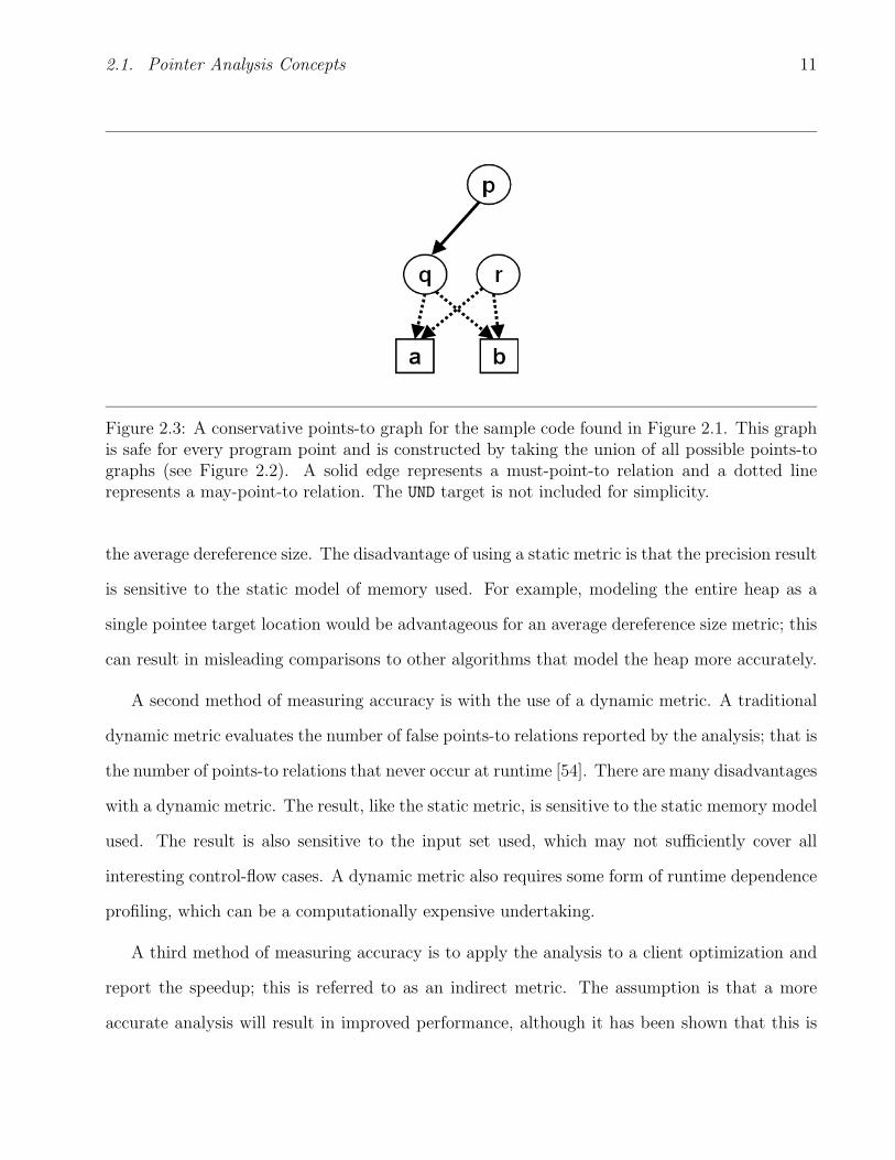
2.3 A conservative points-to graph for the sample code found in Figure 2.1. This
graph is safe for every program point and is constructed by taking the union of
all possible points-to graphs (see Figure 2.2). A solid edge represents a must-
point-to relation and a dotted line represents a may-point-to relation. The UND
target is not included for simplicity. . . . . . . . . . . . . . . . . . . . . . . . . . 11
2.4 Sample code, and the resulting points-to graphs at program point S5 with various
flavors of control-flow sensitivity. . . . . . . . . . . . . . . . . . . . . . . . . . . 13
2.5 Sample code, and the resulting points-to graphs at program point S3 for various
flavors of context sensitivity. . . . . . . . . . . . . . . . . . . . . . . . . . . . . . 14
2.6 An example illustrating the difference between using an alias graph representation
or a points-to representation. Both graphs are flow sensitive and representative
of the state of the pointers p and q at program point S5. This examples shows
why an alias representation can be more accurate. . . . . . . . . . . . . . . . . . 17
ix

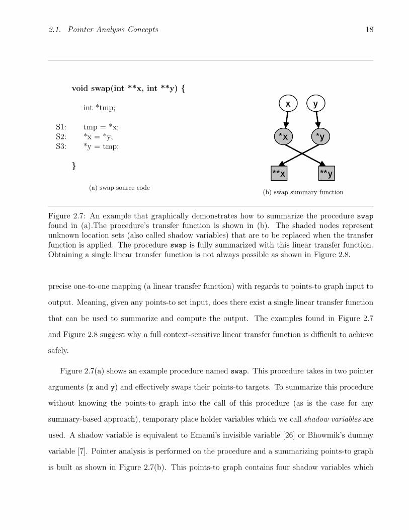
2.7 An example that graphically demonstrates how to summarize the procedure swap
found in (a).The procedure’s transfer function is shown in (b). The shaded nodes
represent unknown location sets (also called shadow variables) that are to be
replaced when the transfer function is applied. The procedure swap is fully sum-
marized with this linear transfer function. Obtaining a single linear transfer
function is not always possible as shown in Figure 2.8. . . . . . . . . . . . . . . 18
2.8 An example that graphically demonstrates how to summarize the procedure
alloc found in (a). The procedure’s transfer functions for 3 different input cases
are shown in (b), (c), and (d). For this example, (d) can be used as a safe linear
transfer function for all 3 input cases, although this may introduce many spurious
points-to relations. . . . . . . . . . . . . . . . . . . . . . . . . . . . . . . . . . . 19
2.9 Different types of flow insensitive points-to analyses. All three points-to graphs
are flow insensitive and therefore safe for all program points. . . . . . . . . . . . 23
2.10 Example on an instruction level data speculative optimization using the EPIC
instruction set. If the compiler is fairly confident that the pointers p and q do not
alias, then the redundant load instruction y = *p can be eliminated speculatively
and replaced with a copy instruction y = w. The copy instruction can then be
hoisted above the store *q = x to increase ILP and enable other optimizations.
To support this optimization, extra code for checking and recovering in the event
of failed speculation is inserted (shown in bold). . . . . . . . . . . . . . . . . . . 27
2.11 TLS program execution, when the original sequential program is divided into two
epochs (E1 and E2). . . . . . . . . . . . . . . . . . . . . . . . . . . . . . . . . . 29
3.1 In this sample program, global pointers a and b are assigned in various ways. The
if statement at S3 is taken with probability 0.9, the if statement at S13 is taken
with a probability of 0.01, and the while loop at S5 iterates exactly 100 times. . 35
x

3.2 This is a points-to graph and the corresponding probabilistic points-to graph
associated with the program point after S4 and initially into S5 (PS5) in the
example found in figure 3.1. A dotted arrow indicates a maybe points-to relation
whereas a solid arrow denotes a definite points-to relation. UND is a special location
set used as the sink target for when a pointer’s points-to target is undefined. . . 37
3.3 Fundamental PPA Equation . . . . . . . . . . . . . . . . . . . . . . . . . . . . . 39
3.4 Control flow possibilities . . . . . . . . . . . . . . . . . . . . . . . . . . . . . . . 47
4.1 The LOLIPoP infrastructure. . . . . . . . . . . . . . . . . . . . . . . . . . . . . 55
4.2 In the simple program found in (a), the function swap is called from foo. The
refactored code in (b) is a version of (a) with UND termination applied. The
SMM pass conceptually promotes all function parameters into global variables.
All location sets are assigned to point at the undefined location set when they
are no longer needed. . . . . . . . . . . . . . . . . . . . . . . . . . . . . . . . . 59
5.1 Average dereference size comparison with GOLF for the SPECInt95 benchmarks:
L is LOLIPoP, and G is GOLF. LOLIPoP’s results are safe, except for gcc which
reports an unsafe result. LOLIPoP’s results are more accurate than GOLF for
all benchmarks. . . . . . . . . . . . . . . . . . . . . . . . . . . . . . . . . . . . . 70
5.2 SPECint95 - Normalized Average Euclidean Distance (NAED) relative to the
dynamic execution on the ref input set. D is a uniform distribution of points-to
probabilities, Sr is the safe LOLIPoP result using the ref input set, and the U
bars are the unsafe LOLIPoP result using the ref (Ur) and train (Ut) input sets,
or instead using compile-time heuristics (Un). . . . . . . . . . . . . . . . . . . . 73
xi

5.3 SPECint2000 - Normalized Average Euclidean Distance (NAED) relative to the
dynamic execution on the ref input set. D is a uniform distribution of points-to
probabilities, Sr is the safe LOLIPoP result using the ref input set, and the U
bars are the unsafe LOLIPoP result using the ref (Ur) and train (Ut) input sets,
or instead using compile-time heuristics (Un). . . . . . . . . . . . . . . . . . . . 74
A.1 The LOLIPoP infrastructure. . . . . . . . . . . . . . . . . . . . . . . . . . . . . 82
xii

Chapter 1
Introduction
Pointers are powerful constructs in C and other similar programming languages that enable
programmers to implement complex data structures. However, pointer values are often am-
biguous at compile time, complicating program analyses and impeding optimization by forcing
the compiler to be conservative. Many pointer analyses have been proposed which attempt
to minimize pointer ambiguity and enable compiler optimization in the presence of point-
ers [2, 6, 22, 26, 49, 62, 65, 77, 78, 80]. In general, the design of a pointer analysis algorithm is
quite challenging, with many options that trade accuracy for space/time complexity. For ex-
ample, the most accurate algorithms often cannot scale in time and space to accommodate
large programs [26], although some progress has been made recently using binary decision dia-
grams [6, 77,80].
The fact that memory references often remain ambiguous even after performing a thorough
pointer analysis has motivated a class of compiler-based optimizations called speculative op-
timizations. A speculative optimization typically involves a code transformation that allows
ambiguous memory references to be scheduled in a potentially unsafe order, and requires a
recovery mechanism to ensure program correctness in the case where the memory references
were indeed dependent. For example, EPIC instruction sets (eg., Intel’s IA64) provide hardware
1
1.1. Probabilistic Pointer Analysis 2
support that allows the compiler to schedule a load ahead of a potentially-dependent store, and
to specify recovery code that is executed in the event that the execution is unsafe [24,45]. Pro-
posed speculative optimizations that allow the compiler to exploit this new hardware support
include speculative dead store elimination, speculative redundancy elimination, speculative copy
propagation, and speculative code scheduling [20,51,52].
More aggressive hardware-supported techniques, such as thread-level speculation [40, 47,
60, 69] and transactional programming [37, 38] allow the speculative parallelization of sequen-
tial programs through hardware support for tracking dependences between speculative threads,
buffering speculative modifications, and recovering from failed speculation. Unfortunately, to
drive the decision of when to speculate many of these techniques rely on extensive data de-
pendence profile information which is expensive to obtain and often unavailable. Hence we are
motivated to investigate compile-time techniques—to take a fresh look at pointer analysis with
speculative optimizations in mind.
1.1 Probabilistic Pointer Analysis
A conventional pointer analysis deduces for every pair of pointers, at any program point, whether
a points-to relation between them (i) definitely exists, (ii) definitely does not exist, or (iii) maybe
exists. Typically, a large majority of points-to relations are categorized as maybe, especially
if a fast-but-inaccurate approach is used. Unfortunately, many optimizations must treat the
maybe case conservatively, and to ensure correctness cannot optimize. However, speculative
optimizations can capitalize on the maybe case—especially if the likelihood that two pointers
alias can be quantified. In order to obtain this likelihood information, in this thesis we propose
a Probabilistic Pointer Analysis (PPA) that accurately predicts the probability of each points-to
relation at every program point.
1.2. Research Goals 3
1.2 Research Goals
The focus of this research is to develop a Probabilistic Pointer Analysis (PPA) for which we
have the following goals:
1. to accurately predict the probability of each points-to relation at every pointer dereference;
2. to scale to the SPEC 2000 integer benchmark suite [19];
3. to understand potential trade-offs between scalability and accuracy; and
4. to increase the overall understanding of program behaviour.
To satisfy these goals we have developed a PPA infrastructure, called Linear One-Level
Interprocedural Probabilistic Points-to (LOLIPoP), based on an innovative algorithm that is
both scalable and accurate: building on simple (control-flow) edge profiling, the analysis is
both one-level context and flow sensitive, yet can still scale to large programs. The key to the
approach is to compute points-to probabilities through the use of linear transfer functions that
are efficiently encoded as sparse matrices. LOLIPoP is very flexible, allowing us to explore the
scalability/accuracy trade-off space.
1.3 Organization
The remainder of this dissertation is organized as follows. In Chapter 2 the background material
and related work in the fields of pointer analysis and pointer analysis for speculative optimization
are described. In Chapter 3 the probabilistic pointer analysis algorithm is described. Chapter 4
describes the LOLIPoP infrastructure, including the practical implementation details and the
design tradeoffs. Chapter 5 evaluates the efficiency and accuracy of the LOLIPoP infrastructure,
and Chapter 6 concludes by summarizing the dissertation, naming its contributions, and listing
future extensions of this work.

Chapter 2
Background
This chapter presents the background material and related work in the fields of pointer analysis
and pointer analysis for speculative optimization. The organization of this chapter is divided into
four main areas: Section 2.1 introduces the basic concepts and terminology involved in pointer
analysis research; Section 2.2 describes some of the traditional approaches used to perform
pointer analysis and outlines the strengths and drawbacks of the various approaches; Section 2.3
discusses various speculative optimizations that have been proposed to aggressively exploit overly
conservative pointer analysis schemes; and finally Section 2.4 describes more recently proposed
program analysis techniques that aid speculative optimizations.
2.1 Pointer Analysis Concepts
A pointer is a programming language datatype whose value refers directly to (or points-to) the
address in memory of another variable. Pointers are powerful programming constructs that are
heavily utilized by programmers to realize complex data structures and algorithms in C and
other similar programming languages. They provide the programmer with a level of indirection
when accessing data stored in memory. This level of indirection is very useful for two main
4

2.1. Pointer Analysis Concepts 5
Table 2.1: Pointer Assignment Instructions
α = &β Address-of Assignment
α = β Copy Assignment
α = *β Load Assignment
*α = β Store Assignment
reasons: (1) it allows different sections of code to share information easily; and (2) it allows for
the creation of more complex “linked” dynamic data structures such as linked lists, trees, hash
tables, etc. For the purposes of this discussion, the variable that the pointer points to is called
a pointee target. A points-to relation between a pointer and a pointee is created with the unary
operator ‘&’, which gives the address of a variable. For example, to create a points-to relation
〈∗α, β〉 between a pointer α and a target β, the following assignment is used α = &β. The
indirection or dereference operator ‘*’ gives the contents of an object pointed to by a pointer
(i.e. the pointee’s contents). The assignment operation ‘=’ when used between two pointers,
makes the pointer on the left side of the assignment point to the same target as the pointer on
the right side. Table 2.1 describes the four basic instructions that can be used to create points-to
relations. All other pointer assigning instructions can be normalized into some combination of
these four types. Figure 2.1 is a C source code example that demonstrates how pointers can be
assigned and used.
In this example found in Figure 2.1, there are three pointer variables (p, q, and r) and three
pointee target variables that can be pointed at (a, b and q). Any variable, including a pointer,
whose address is taken using the ‘&’ operator is defined as a pointee target. Initially, at program
point S1, all three pointers (p, q, and r) are uninitialized. A special undefined pointee target,

2.1. Pointer Analysis Concepts 6
void main() {
int a = 1, b = 2;int **p, *q, *r;
S1: q = &a;S2: r = q;S3: p = &q;S4: *p = &b;S5: r = *p;
S6: **p = 3;S7: *r = 4;
...
}
Figure 2.1: Sample C code that uses pointers.
denoted ‘UND’, is used as the target of an uninitialized pointer. Therefore, at program point S1,
the points-to relations that exist are: 〈∗p, UND〉, 〈∗q, UND〉, and 〈∗r, UND〉. At program point S1,
the pointer q is assigned to point to the target a using an address-of assignment. Statement
S1 has the following two side effects: (1) the points-to relation 〈∗q, UND〉 is killed, and (2) the
points-to relation 〈∗q, a〉 is generated. At program point S2, the copy assignment instruction
assigns the pointer r to point to the target of pointer q. At S2, The pointer q has a single target,
which is a. Therefore, S2 kills the points-to relation 〈∗r, UND〉 and creates the points-to relation
〈∗r, a〉. At S3, there is another address-of assignment that assigns the double pointer p to point
to the target q, which is itself is a pointer. This instruction creates the following two points-to
relations 〈∗p, q〉 and 〈∗ ∗ p, a〉1. The instruction at S4 is a store assignment. Since it can be
proven that at program point S4 the pointer p can only point to q, S4 kills the points-to relation
1A double pointer points-to relation such as this one is often ignored and not tracked because it can beinferred from the other points-to relations in the set.

2.1. Pointer Analysis Concepts 7
〈∗q, a〉 and creates the points-to relation 〈∗q, b〉. The instruction at S5 is a load assignment that
assigns r to point to the target of ∗p, which is the target of q, which is b. Therefore, at S6,
the following points-to relations are said to exist: 〈∗p, q〉, 〈∗q, b〉 and 〈∗r, b〉. An analysis such
as this, that tracks the possible targets that a pointer can have, is referred to as a points-to
analysis. A safe points-to analysis reports all possible points-to relations that may exist at any
program point.
2.1.1 Pointer Alias Analysis and Points-To Analysis
A pointer alias analysis determines, for every pair of pointers at every program point, whether
two pointer expressions refer to the same storage location or equivalently store the same ad-
dress. A pointer alias analysis algorithm will deduce for every pair of pointers one of three
classifications: (i) definitely aliased, (ii) definitely not aliased, or (iii) maybe aliased. A points-to
analysis, although similar, is subtly different. A points-to analysis attempts to determine what
storage locations or pointees a pointer can point to—the result can then be used as a means
of extracting or inferring pointer aliasing information. The main differences between an alias
analysis and a points-to analysis are the underlying data structure used by the algorithm and
the output produced. The analysis type has consequences in terms of precision and algorithm
scalability—these will be discussed further in section 2.1.6. The terms pointer alias analysis and
points-to analysis are often times incorrectly used interchangeably. The broader term of pointer
analysis is typically used to encapsulate both.
2.1.2 The Importance of and Difficulties with Pointer Analysis
Pointer analysis does not improve program performance directly, but is used by other optimiza-
tions and is typically a fundamental component of any static analysis. Static program analysis
aims at determining properties of the behaviour of a program without actually executing it.

2.1. Pointer Analysis Concepts 8
It analyzes software source code or object code in an effort to gain understanding of what the
software does and establish certain correctness criteria to be used for various purposes. These
purposes include, but are not limited to: optimizing compilers, parallelizing compilers, support
for advanced architectures, behavioral synthesis, debuggers and other verification tools. One
of the main challenges of any program analysis is to safely determine what memory locations
the program is attempting to access at any read or write instruction, and this problem be-
comes substantially more difficult when memory is accessed through a pointer. In order to gain
useful insight, a pointer analysis is often required. Complicating things further, the degree of
accuracy required by a pointer analysis technique is dependent on the actual program analysis
being performed [44]. For example, in the sample code presented in Figure 2.1, an optimizing
compiler or a parallelizing compiler would want to know whether the statements at S6 and S7
accessed the same memory locations. If the static analyzer could prove that all load and store
operations were independent, then the statements could potentially be reordered or executed in
parallel in order to improve performance. Many advanced architectures, behavioral/hardware
synthesis tools [34, 64, 76] and dataflow processors [63, 71] attempt to reduce the pressure on
a traditional cache hierarchy by prepartitioning memory accesses into different memory banks.
These applications rely on a static analysis that is able to safely predetermine at compile time
which memory accesses are mapped to which memory banks. The accuracy of pointer analysis
is not as important for this purpose of memory partitioning [64]. As a final example a debugger
uses pointer analysis to detect uninitialized pointers or memory leaks.
Currently, developing both an accurate and scalable pointer analysis algorithm is still re-
garded as an important yet very complex problem. Even without dynamic memory allocation,
given at least four levels of pointer dereferencing (i.e. allowing pointer chains to be of length 4)
the problem has been shown to be PSPACE Complete [49] and to be NP Hard given at least
two levels of pointer dereferencing [48]. Given these results, it is very unlikely that there are
precise, polynomial time algorithms for the C programming language. Although, there are many

2.1. Pointer Analysis Concepts 9
different solutions that trade off some precision for scalability. These tradeoffs are discussed
further in Section 2.1.6.
2.1.3 Static Memory Model
To perform any pointer analysis, an abstract representation of addressable memory called a
static memory model must be constructed. For the remainder of this dissertation, it is assumed
that a static memory model is composed of location sets [78]2. A location set can represent one or
more real memory locations, and can be classified as a pointer, pointee, or both. A location set
only tracks its approximate size and the approximate number of pointers it represents, allowing
the algorithm used to abstract away the complexities of aggregate data structures and arrays
of pointers. For example, fields within a C struct can either be merged into one location set, or
else treated as separate location sets.
2.1.4 Points-To Graph
A points-to relation between a pointer α and a pointee target β is denoted as such 〈∗α, β〉. This
notation signifies that the dereference of variable α and variable β may be aliased. A points-to
graph is typically used in a points-to analysis algorithm to efficiently encode all possible may
points-to relations. A points-to graph is a directed graph whose vertices represent the various
pointer location sets and pointee target location sets. An edge from node α to the target node
β represents a may-points-to relation 〈∗α, β〉. For certain algorithms, the edge is additionally
annotated as a must points-to edge, if the relation is proven to always persist. Figure 2.2
shows the points-to graphs for the various program points associated with the sample code in
Figure 2.1.
2Note that the term location set itself is not necessarily dependent on this location-set-based model.

2.1. Pointer Analysis Concepts 10
void main() {
int a = 1, b = 2;int **p, *q, *r;
S1: q = &a;S2: r = q;S3: p = &q;S4: *p = &b;S5: r = *p;
S6: **p = 3;S7: *r = 4;
...
}
(a) Sample program from Figure 2.1
(b) S1 (c) S2
(d) S3 (e) S4
(f) S5 (g) S6
Figure 2.2: The points-to graphs corresponding to the different program points in the samplecode found in Figure 2.1.
2.1.5 Pointer Analysis Accuracy Metrics
The conventional way to compare the precision of different pointer analyses is by using either
a static or dynamic metric. A static metric (also called a direct metric) asserts, without ever
executing the program, that a pointer analysis algorithm X is more precise than an algorithm
Y if the point-to graph generated by the algorithm X is a subset of Y, given an equal model of
memory. Many researchers [22,26,43,49] estimate precision by measuring the cardinality of the
points-to set for each pointer dereference expression, and then calculate the average—in short,
2.1. Pointer Analysis Concepts 11
Figure 2.3: A conservative points-to graph for the sample code found in Figure 2.1. This graphis safe for every program point and is constructed by taking the union of all possible points-tographs (see Figure 2.2). A solid edge represents a must-point-to relation and a dotted linerepresents a may-point-to relation. The UND target is not included for simplicity.
the average dereference size. The disadvantage of using a static metric is that the precision result
is sensitive to the static model of memory used. For example, modeling the entire heap as a
single pointee target location would be advantageous for an average dereference size metric; this
can result in misleading comparisons to other algorithms that model the heap more accurately.
A second method of measuring accuracy is with the use of a dynamic metric. A traditional
dynamic metric evaluates the number of false points-to relations reported by the analysis; that is
the number of points-to relations that never occur at runtime [54]. There are many disadvantages
with a dynamic metric. The result, like the static metric, is sensitive to the static memory model
used. The result is also sensitive to the input set used, which may not sufficiently cover all
interesting control-flow cases. A dynamic metric also requires some form of runtime dependence
profiling, which can be a computationally expensive undertaking.
A third method of measuring accuracy is to apply the analysis to a client optimization and
report the speedup; this is referred to as an indirect metric. The assumption is that a more
accurate analysis will result in improved performance, although it has been shown that this is

2.1. Pointer Analysis Concepts 12
not always the case [22,23,44] and therefore an indirect metric may be disadvantageous as well.
Hind addresses this accuracy metric problem [42] and argues that the best way to measure and
compare pointer analysis precision is to concurrently use all three types: static, dynamic, and
indirect.
2.1.6 Algorithm Design Choices
There are many factors and algorithm design choices that cause a pointer analysis X to be more
accurate than a pointer analysis Y. Typically, when making algorithm design choices there exists
a tradeoff between algorithm scalability (in time and space) and accuracy. Some of the major
design considerations are [42]:
• flow-sensitivity,
• context-sensitivity,
• aggregate modeling / field-sensitivity,
• heap modeling, and
• alias representation.
A flow-sensitive pointer analysis takes into account the order in which statements are
executed when computing points-to side effects. It is normally realized through the use of
strong/weak updates applied to a data flow analysis (DFA) [1, 56] framework, which requires
repeated calculations on a control flow graph until a fixed point solution is found. The analysis is
considered to be highly precise; however, the analysis is generally regarded as too computation-
ally intensive for two reasons: (1) Pointer analysis generally requires a forward and backward
interprocedural DFA, which is not feasible for large programs [70]; and (2) it also requires that
a points-to graph be calculated for every program point. Because of the exponential number

2.1. Pointer Analysis Concepts 13
void fsTest(int x) {
int a, b, c, d;int *p;
S1: p = &a;S2: p = &b;
if(x)S3: p = &c;
if(x)S4: p = &d;
S5: *p = 0;
}
(a) Sample program
(b) Flow Insensitive
(c) Flow Sensitive
(d) Path Sensitive
Figure 2.4: Sample code, and the resulting points-to graphs at program point S5 with variousflavors of control-flow sensitivity.
of program points associated with an interprocedural analysis, achieving a scalable solution is
difficult. A further and more ambitious approach is a path sensitive analysis, which requires
that each non-cyclic path be analyzed individually; a means of correlating control dependences
is required to prune away invalid control flow paths. Figure 2.4 shows a sample program and
depicts the different points-to graphs created by the three different approaches.
A context-sensitive pointer analysis distinguishes between the different calling contexts of
a procedure. The implication is that the points to side effects on any given path of the call
graph are treated uniquely, in contrast to a context-insensitive pointer analysis which merges all
the calling contexts of a procedure when summarizing the points-to side effects. We discuss the

2.1. Pointer Analysis Concepts 14
int *retParam(int *x) {return x;
}
void csTest() {
int a, b;int *p, *q;
S1: p = retParam(&a);S2: q = retParam(&b);
S3: *p = 0; *q = 0;
}
(a) Sample program
(b) Context Insensitive
(c) Context Sensitive
Figure 2.5: Sample code, and the resulting points-to graphs at program point S3 for variousflavors of context sensitivity.
difficulties associated with a context sensitive analysis later in Section 2.1.7, and in Sections 2.2.2
and 2.2.3 we describe various methods that have been proposed for overcoming these difficulties.
Figure 2.5 shows a sample program and depicts the two different points-to graphs created by a
context insensitive and a context sensitive analysis.
A third factor affecting accuracy is aggregate modeling or field-sensitivity. Aggregate
structures with multiple pointer type fields, such as arrays of pointers or C structs can be
handled specially. Pointers within structs are merged and handled as a single pointer in a field-
insensitive analysis. Conversely, a field-sensitive analysis handles every field and subsequently
subfield as a separate and unique field. This approach additively requires a means of handling
recursive data structures. Similarly, an array of pointers can be handled as a single node or each
array element could be treated as a unique pointer field. Treating each array node uniquely

2.1. Pointer Analysis Concepts 15
creates many complications because of array subscript uncertainty. A third option, proposed
by Emami [26], is to represent arrays (both pointers and pointee targets) with two location
sets. One of the location sets represents the first element of the array and the second element
represents the remainder of the array. This added information enables a client analysis to be
more aggressive when performing array subscript dependence analysis.
Heap modeling is another important, yet often neglected, design decision to be considered
when performing any pointer analysis. A means of dealing with pointee targets created by
dynamic allocation library calls such as malloc and calloc in C is required. The simplest and
most inaccurate approach is to merge all heap allocation callsites into one location set. The
most common approach is callsite allocation, which treats each individual callsite allocation
program point as a unique location set target. This approach is considered to produce precise
results in most cases; although, when a programmer uses a custom allocator [5,11] it essentially
degrades the analysis into a heap-merged approach. A more precise approach that addresses
this custom allocator issue is to assign a unique location set for every unique context path
to every allocation callsite [43, 50, 57]. Other aggressive shape analysis techniques have also
been proposed. A shape analysis technique attempts to further disambiguate dynamic memory
location sets by categorizing the underlying data structure created by the allocation callsite into
a List, Tree, DAG, or Cyclic Graph [33].
Alias representation is yet another factor to be considered by any pointer analysis al-
gorithm. Alias representation signifies what type of data structure is used to track aliasing
information. There are two basic representation types:
• alias pairs, and
• points-to relations.
A complete alias-pairs representation stores all alias pairs explicitly, such as the one used by
Landi [49]. A compact alias-pairs representation stores only basic alias pairs, and derives new

2.1. Pointer Analysis Concepts 16
alias pairs by dereference, transitivity and commutativity. The most common representation
is to store points-to relation pairs to indicate that one variable is pointing to another. Addi-
tionally, the representation can choose to distinguish between must-alias and may-alias pairs;
this information is very useful for a flow-sensitive analysis that uses strong and weak updates.
Figure 2.6 demonstrates a sample program created to illustrate the difference between the two
representations. The flow sensitive pointer alias graph and points-to graph corresponding to
program point S5 is shown in Figure 2.6 (b) and (c) respectively. If the compiler wanted to
know, at program point S5, do the pointers p and q alias? The alias-pairs representation ap-
proach would output definitely no, whereas the point-to representation approach would answer
with maybe. The alias analysis approach is considered to be slightly more precise but relatively
much more expensive in terms of complexity.
2.1.7 Context Sensitivity Challenges
Context sensitivity is regarded as the most important contributor towards achieving an accurate
pointer analysis. Conceptually, context sensitivity can be realized by giving each caller its own
copy of the function being called. Two distinct approaches have been proposed:
• cloning-based analysis, and
• summary-based analysis.
The simplest way of achieving context sensitivity is through function cloning. In a cloning-
based analysis every path through the call graph is cloned or conceptually inlined, and then a
context-insensitive algorithm on the expanded call graph is performed. This expanded call graph
is called an invocation graph [26]. This technique is a simple way of adding context sensitivity to
any analysis. The problem with this technique is that the invocation graph, if not represented
sensibly, can blow up exponentially in size.

2.1. Pointer Analysis Concepts 17
void aliasRepTest() {
int a, b, c;int *p, *q;
if(x) {S1: p = &a;S2: q = &b;
} else {S3: p = &b;S4: q = &c;
}
S5: *p = 0; *q = 1;
}
(a) Alias Representation Example
(b) Pointer Alias Graph
(c) Points-To Graph
Figure 2.6: An example illustrating the difference between using an alias graph representationor a points-to representation. Both graphs are flow sensitive and representative of the state ofthe pointers p and q at program point S5. This examples shows why an alias representation canbe more accurate.
In a summary-based analysis, a summary (or a transfer function) which summarizes the
effects of a procedure is obtained for each procedure. The algorithm usually has two phases:
(i) a bottom-up phase in which the summaries for each procedure are collected using a reverse
topological traversal of the call graph; and (ii) a top-down phase in which points-to information
is propagated back down in a forward topological traversal through the call graph. This two
phased approach is very advantageous for any analysis that can easily summarize the effects of
a procedure. Unfortunately, for a full context-sensitive pointer analysis, this approach has not
yet been shown to scale to large programs—mainly because it is difficult to concisely summarize
the points-to side effects of a procedure. The difficulty lies in the inability to compute a safe and
2.1. Pointer Analysis Concepts 18
void swap(int **x, int **y) {
int *tmp;
S1: tmp = *x;S2: *x = *y;S3: *y = tmp;
}
(a) swap source code(b) swap summary function
Figure 2.7: An example that graphically demonstrates how to summarize the procedure swap
found in (a).The procedure’s transfer function is shown in (b). The shaded nodes representunknown location sets (also called shadow variables) that are to be replaced when the transferfunction is applied. The procedure swap is fully summarized with this linear transfer function.Obtaining a single linear transfer function is not always possible as shown in Figure 2.8.
precise one-to-one mapping (a linear transfer function) with regards to points-to graph input to
output. Meaning, given any points-to set input, does there exist a single linear transfer function
that can be used to summarize and compute the output. The examples found in Figure 2.7
and Figure 2.8 suggest why a full context-sensitive linear transfer function is difficult to achieve
safely.
Figure 2.7(a) shows an example procedure named swap. This procedure takes in two pointer
arguments (x and y) and effectively swaps their points-to targets. To summarize this procedure
without knowing the points-to graph into the call of this procedure (as is the case for any
summary-based approach), temporary place holder variables which we call shadow variables are
used. A shadow variable is equivalent to Emami’s invisible variable [26] or Bhowmik’s dummy
variable [7]. Pointer analysis is performed on the procedure and a summarizing points-to graph
is built as shown in Figure 2.7(b). This points-to graph contains four shadow variables which

2.1. Pointer Analysis Concepts 19
void alloc(int **x, int **y) {
S1: *x = (int*)malloc(sizeof(int));
}
(a) alloc source code
(b) alloc summary function(*x is not aliased to *y)
(c) alloc summary function(*x definitely aliased to *y)
(d) alloc summary function(*x might be aliased to *y)
Figure 2.8: An example that graphically demonstrates how to summarize the procedure alloc
found in (a). The procedure’s transfer functions for 3 different input cases are shown in (b),(c), and (d). For this example, (d) can be used as a safe linear transfer function for all 3 inputcases, although this may introduce many spurious points-to relations.
are the shaded nodes within the points to graph. When analyzing a call to the swap procedure,
the shadow variables within the transfer function are replaced with the input-parameter location
set variables. The resulting transfer function represents the side effects obtained with a call to
the swap procedure. This swap procedure is an ideal candidate procedure for a summary based
approach because the transfer function is linear, meaning the side effects are independent of the
input points-to graph. Figure 2.8 illustrates an example where this is not the case.
Figure 2.8(a) shows an example procedure named alloc. This procedure also takes in two
pointer arguments (x and y), and the pointer y is allocated to the dynamic heap location set
named heap s1. Figure 2.8(b) illustrates the intuitive summarizing function which reassigns the

2.1. Pointer Analysis Concepts 20
shadow pointer *x to point to the new location set heap s1 and the shadow pointer *y remains
unchanged. Unfortunately, in the unlikely event that the shadow variables *x and *y are aliased
(refer to the same variable) then this summarizing function is incorrect. In the event that *x
and *y definitely alias, then the summarizing function found in Figure 2.8(b) should be applied,
which additionally reassigns *y to point to heap s1. In the event of a may-alias relation between
*x and *y, Figure 2.8(c) depicts the transfer function that should be applied. This problem of
aliasing input pointer arguments is referred to as Shadow Variable Aliasing (SVA). All summary
based approaches must somehow solve this SVA problem.
The SVA problem stems from the use of call by reference parameters and global variables
passing between procedures which introduce aliases, an effect where two or more l-values [1] refer
to the same location set at the same program point. More precisely aliases created by multiple
levels of dereferencing impede summary-based pointer analyses; i.e. pointers with k levels of
dereferencing where k > 1 and k is the maximum level of pointer dereferencing. Ramalingam [58]
shows that solving the may-alias problem for k > 1 level pointer is undecidable. However, if
k = 1 the problem has been shown to be almost trivial [8,49]. Most summary based approaches
attempt to somehow map the k = n problem into a k = 1 problem3. There are four known
approaches to achieving this mapping.
1. Perform a one-level analysis n times [26].
2. For each incoming alias pattern, specialize each procedure summary for all possible input
alias patterns [78]; this approach is called a Partial Transfer Function (PTF) approach.
3. Hoist and inline multi-level pointer assignment instructions from caller to callee until they
can be resolved into a one-level pointer assignment instruction [9].
4. Summarize each procedure using a single safe [12] or unsafe [7] summary function.
3n represents the maximum level of dereferencing found in the program

2.2. Conventional Pointer Analysis Techniques 21
These approaches will be further discussed in Section 2.2.
2.2 Conventional Pointer Analysis Techniques
Pointer analysis is a well-researched problem and many algorithms have been proposed, yet
no one approach has emerged as the preferred choice [44]. A universal solution to pointer
analysis is prevented by the large trade-off between precision and scalability as described in
Section 2.1.6. The most accurate algorithms are both context-sensitive and control-flow-sensitive
(CSFS) [26,49,78]; however, it has yet to be demonstrated whether these approaches can scale to
large programs. Context-insensitive control-flow-insensitive (CIFI) algorithms [2, 65] can scale
almost linearly to large programs, but these approaches are regarded as overly conservative and
may impede aggressive compiler optimization. Several approaches balance this trade-off well
by providing an appropriate combination of precision and scalability [6, 22, 77, 80], although
their relative effectiveness when applied to different aggressive compiler optimizations remains
in question.
2.2.1 Context-insensitive Flow-insensitive (CIFI) Algorithms
The simplest and most common types of pointer analysis algorithms are typically both context-
insensitive and flow-insensitive (CIFI). Not surprisingly, there exists many different types of
CIFI algorithms. Currently, most commercially available compilers simply use an address-taken
CIFI pointer analysis. This type of analysis simply asserts that every object that has its address
taken may be the target of any pointer object. This is obviously a very imprecise approach,
although it is quite effective at improving the programs performance when applied to a client
optimization relative to using no pointer analysis [44].
The two classic approaches to realizing an efficient context-insensitive flow-insensitive (CIFI)
analysis are:

2.2. Conventional Pointer Analysis Techniques 22
• inclusion based, and
• unification based.
An inclusion based analysis treats every pointer assignment instruction as a constraint equa-
tion and iteratively solves for the points-to graph by repeatedly performing a transitive closure
on the entire graph, until a fixed solution is realized. Andersen [2] initially proposed a sim-
ple and intuitive CIFI inclusion based pointer analysis with worst case complexity of O(n3);
where n is the size of the program. Fahndrich, et al [27] improved on the runtime of Andersen’s
pointer analysis by collapsing cyclic constraints into a single node, and by selectively propagating
matching constraints. With this optimized approach, they demonstrated orders of magnitude
improvement in analysis runtime. Rountev and Chandra [61] also proposed a similar and more
aggressive algorithm for collapsing cyclical constraints and avoiding duplicate computations.
A unification based approach is a much more scalable, yet slightly less accurate approach
to performing a FICI analysis. In a unification based approach, location set nodes within the
points-to graph are merged such that every node within the graph can only point to a single
other node. This merge operation eliminates the transitive closure operation required by the
inclusion based approach and therefore allows for linear scaling. Steensgaard [65] proposed
the first unification based algorithm, which runs in almost linear time. The algorithm uses
Tarjan’s union-find data structure [73] to efficiently perform the analysis. The disadvantage of
a unification approach is that it may introduce many spurious point-to relations as is the case
in the example found in Figure 2.9. In this example, the unification based approach creates the
following spurious (false) points-to relations: 〈∗r, b〉, 〈∗s, a〉, and〈∗q, b〉.
2.2.2 Context-sensitive Flow-sensitive (CSFS) Algorithms
The most precise pointer analysis algorithms are typically both context-sensitive and flow-
sensitive (CSFS). Emami, Ghiya, and Hendren [26] introduced the invocation graph and pro-

2.2. Conventional Pointer Analysis Techniques 23
void main() {
int **p, *q, *r, *s;int a, b;
S1: q = &a;S2: p = &r;S3: r = &a;S4: p = &s;S5: s = &b;
}
(a) Sample program
(b) address-taken (c) inclusion based
(d) unification based
Figure 2.9: Different types of flow insensitive points-to analyses. All three points-to graphs areflow insensitive and therefore safe for all program points.
posed a cloning-based CSFS points-to analysis for C programs. The analysis was designed to be
very accurate for disambiguating pointer references that access stack based memory locations.
The analysis is field sensitive and maps each stack variables to a unique location set, including
locals, parameters, and globals. Arrays are modeled as two location sets, one representing the
first element of the array and the other representing the rest of the array. The heap is modeled
inaccurately and allocated a single location set. Pointers through indirect calls are handled iter-
atively using a transitive closure. Additionally, the analysis tracks both may and must points-to
relationships and use both strong and weak updates while propagating a flow sensitive points-
to graph. Similar to a summary-based approach, Emami’s approach caches the side-effects of
each function call for reuse. The shadow variable aliasing problem was handled by repeating
their one-level analysis n times, where n is the maximum level of dereferencing used. Although
2.2. Conventional Pointer Analysis Techniques 24
this analysis dramatically improves the precision in relation to the CIFI analysis, the programs
analyzed were very small and in general the analysis is not expected to scale to larger programs.
Wilson and Lam [78] proposed a summary based CSFS analysis that recognized that many
of the calling contexts were quite similar in terms of alias patterns between the parameters.
As such, they proposed the use of a partial transfer function (PTF) to capture the points-to
information for each procedure. A PTF is a set of linear transfer functions representative of all
possible aliasing scenarios that a given procedure may encounter. The PTF does this by using
temporary location sets to represent the initial point-to information of parameters, and uses
the PTF to derive the final point-to information of the procedure. For the benchmarks used,
they showed only a 30% increase in the number of transfer functions needed. This analysis also
allocated each stack variable and global a unique location set and, in addition, they mapped
each heap allocation callsite to a unique location set. This pointer analysis was shown to run
on benchmarks as large as five thousand lines of code.
Chaterjee, Ryder, and Landi [12] proposed a modular context-sensitive pointer analysis,
using the same static memory model as Wilson and Lam [78], but fully summarizing each
procedure using a single safe transfer function. By detecting strongly connected components
in the call graph, and analyzing them separately they showed space improvements, but no
results on benchmarks larger than 5000 lines of code. Cheng and Hwu [15] extended [12] by
implementing an access path based approach, and partial context-sensitivity, distinguishing
between the arguments at only selected procedures. They demonstrated scalability to hundreds
of thousands of lines of code.
2.2.3 Context-sensitive Flow-insensitive (CSFI) Algorithms
Fahndrich, Rehof, and Das [28] proposed a one-level unification based CSFI pointer analysis.
This analysis distinguishes between the incoming calls to a given procedure, rather than expand
2.3. Speculative Optimization 25
each path in the call graph. The authors showed that this analysis can analyze hundreds of thou-
sands of lines of code in minutes, and showed precision improvements over the flow-insensitive
context-insensitive unification based analysis. Das also proposed a summary-based generalized
one level flow (GOLF) [22] analysis which adds limited context sensitivity to his unification
based CIFI one level flow idea from [21]. GOLF is field-insensitive and uses callsite alloca-
tion. It is regarded as a relatively precise algorithm that scales well beyond the SPECint95 [19]
benchmarks.
Some progress has also been made recently using a binary decision diagram (BDD) [6,77,80]
data structure to efficiently solve the pointer analysis problem accurately. A BDD based ap-
proach uses Bryant’s [10] Reduced Order Binary Decision Diagram (ROBDD, also called BDD)
to solve the pointer analysis problem using superposition. Similar to the dynamic programming
paradigm, a BDD is able encode and solve exponential problems, on average (and not in the
worst case), in linear time if repetition or duplication exists. The CSFI pointer analysis problem
is formulated using a cloning based approach and the invocation graph is encoded using boolean
logic into a BDD. The problem is then solved quite efficiently because much of the analysis on
an invocation graph involves analyzing duplicated context paths.
2.3 Speculative Optimization
Studies suggest that a more accurate pointer analysis does not necessarily provide increased
optimization opportunities [22, 23, 44] because ambiguous pointers will persist. The fact that
memory references often remain ambiguous even after performing a thorough pointer analy-
sis has motivated a class of compiler-based optimizations called data speculative optimizations.
A data speculative optimization typically involves a code transformation that allows ambigu-
ous memory references to be scheduled in a potentially unsafe order, and requires a recovery
mechanism to ensure program correctness in the case where the memory references were indeed

2.3. Speculative Optimization 26
dependent. Speculative optimizations benefit from pointer analysis information that quantifies
the likelihood of data dependences and is therefore the target use of the probabilistic pointer
analysis proposed by this thesis. Proposed forms of data speculative optimization can be catego-
rized into two classes: (1) Instruction Level Data Speculation and (2) Thread Level Speculation
(TLS). Instruction level data speculation attempts to increase the available instruction level
parallelism or eliminate unnecessary computation by using potentially unsafe compiler trans-
formations. Thread level speculation allows the compiler to speculatively parallelize sequential
programs without proving that it is safe to do so.
2.3.1 Instruction Level Data Speculation
Due to the complexity of scaling the conventional superscalar out-of-order execution paradigm,
the processor industry started to re-examine instruction sets which explicitly encode multiple
operations per instruction. The main goal is to move the complexity of dynamic scheduling of
multiple instructions from the hardware implementation to the compiler, which does the instruc-
tion scheduling statically. One main drawback to this approach is that to extract instruction
level parallelism statically, information regarding aliasing memory references becomes essential.
As described in Section 2.2, even if the most accurate techniques are used ambiguous pointers
will persist. As a direct consequence, HP and Intel have recently introduced a new style of in-
struction set architecture called EPIC (Explicitly Parallel Instruction Computing), and a specific
architecture called the IPF (Itanium Processor Family). EPIC is a computing paradigm that
began to be researched in the 1990s. EPIC instruction sets (eg., Intel’s IA64) provide hardware
support that allows the compiler to schedule a load ahead of a potentially-dependent store, and
to specify recovery code that is executed in the event that the execution is unsafe [24,45].
The IPF uses an Advanced Load Address Table (ALAT) to track possibly dependent load and
store operations at runtime. The ALAT is a set-associative structure accessed with load/store

2.3. Speculative Optimization 27
addresses. The IA64 instruction set provides four instructions that interface with the ALAT to
enable many different kinds of speculative optimization: a speculative load (ld.s), a speculation
check (chk.s) an advanced load (ld.a), and an advanced load check (chk.a). Figure 2.10
illustrates a simple and relevant example on how data speculative optimization can be realized.
In this example, if the compiler is able to determine with some amount of probabilistic certainty
that pointers p and q do not alias, then it could be beneficial to eliminate the redundant load
instruction and schedule any other dependent instructions earlier to increase the instruction
level parallelism. To realize this speculative optimization an advanced load (ld.a) instruction
is used in place of a normal load, then an advanced load check (chk.a) instruction that specifies
a recovery branch if p and q where to indeed alias at runtime.
Proposed and successful speculative optimizations that allow the compiler to exploit this new
hardware support include speculative dead store elimination, speculative redundancy elimina-
tion, speculative copy propagation, speculative register promotion, and speculative code schedul-
ing [18,20,51,52,55]. Other envisioned and promising potential speculative optimizations include
speculative loop invariant code motion, speculative constant propagation, speculative common
sub-expression elimination and speculative induction variable elimination. To drive the decision
of when it is profitable to speculate, many of these techniques rely on extensive data dependence
profile information [79] which is expensive to obtain, sensitive to the input set used, possibly
inaccurate, and often unavailable. The main drawback is that this type of profiling can be very
expensive since every memory reference needs to be monitored and compared pair-wise to obtain
accurate results. Lin, et al [51, 52] proposed a lower cost alias profiling scheme to estimate the
alias probability and in addition, when alias profiling is unavailable, they used a set of effective,
and arguably a conservative, set of heuristic rules to quickly approximate alias probabilities in
common cases.

2.3. Speculative Optimization 28
w = *p;
*q = x;
y = *p;
z = y * 2;...
(a) original program
ld.a w = [p];
y = w;z = y * 2;...
st [q] = x;
chk.a w, recover;
recover:ld y = [p];z = y * 2;...
(b) speculative version
Figure 2.10: Example on an instruction level data speculative optimization using the EPICinstruction set. If the compiler is fairly confident that the pointers p and q do not alias, thenthe redundant load instruction y = *p can be eliminated speculatively and replaced with a copyinstruction y = w. The copy instruction can then be hoisted above the store *q = x to increaseILP and enable other optimizations. To support this optimization, extra code for checking andrecovering in the event of failed speculation is inserted (shown in bold).
2.3.2 Thread Level Speculation
Performance gained through instruction level data speculation, although promising, is ultimately
limited by the available instruction level parallelism [46]. To overcome this limit, techniques
to exploit more parallelism by extracting multiple threads out of a single sequential program
remains an open and interesting research problem. This parallelism, called Thread-Level Par-
allelism (TLP), requires the compiler to prove statically that either: (a) the memory references
within the threads it extracts are indeed independent; or (b) the memory references within
the threads are definitely dependent and must be synchronized. Ambiguous pointers are again
problematic. To compensate for these shortcomings, aggressive speculative solutions have been

2.3. Speculative Optimization 29
(a) Sequential execution (b) Successful TLS (p!=q) (c) Failed TLS (p==q)
Figure 2.11: TLS program execution, when the original sequential program is divided into twoepochs (E1 and E2).
proposed to assist the compiler.
Hardware-supported techniques, such as thread-level speculation (TLS) [40, 47, 60, 69] and
transactional programming [37, 38] allow the speculative parallelization of sequential programs
through hardware support for tracking dependences between speculative threads, buffering spec-
ulative modifications, and recovering from failed speculation.
TLS allows the compiler to automatically parallelize general-purpose programs by supporting
parallel execution of threads, even in the presence of statically ambiguous data dependences.
The underlying hardware ensures that speculative threads do not violate any dynamic data
dependence and buffers the speculative data until it is safe to be committed. When a dependence
violation occurs, all the speculative data will be invalidated and the violated threads are re-
executed using the correct data. Figure 2.11 demonstrates a simple TLS example.
The sequential program in Figure 2.11(a), is sliced into two threads of work (called epochs),
and labeled as E1 and E2 in Figure 2.11(b) and (c). They are then executed speculatively in
parallel, even though the addresses of the pointers p and q are not known until runtime. In
essence, TLS allows for the general extraction of any potentially available thread-level paral-

2.3. Speculative Optimization 30
lelism. A read-after-write (true) data dependence occurs when p and q both point to the same
memory location. Since the store produces data that will be read by the dependent load, these
store and load instructions need to be executed in the original sequential program order. In
Figure 2.11(b), p and q do not point to the same location. Therefore, speculation is successful
and both speculative threads can commit their results at the end of execution. However, as
shown in Figure 2.11(c), in the unlucky event that both pointers point to the same location, a
true data dependence is detected and a violation occurs. In this case, speculation fails because it
leads to an out-of-order execution of the dependent load-store pair, which violates the sequential
program order. The offending thread is halted and re-executed with the proper data.
There are various proposed thread-level speculation systems that aim at exploiting thread-
level parallelism in sequential programs by using parallel speculative threads. Among all different
types of thread-level speculation systems that have been proposed, there are three common key
components: (i) breaking a sequential program into speculative threads—this task must be done
efficiently to maximize thread-level parallelism and minimize the overhead; (ii) tracking data
dependences—since the threads are executed speculatively in parallel, the system must be able to
determine whether the speculation is successful; (iii) recovering from failed speculation—in the
case when speculation has failed, the system must repair the incorrect architectural states and
data, and discard the speculative work. Different TLS systems have different implementations
of these three components.
In the Multiscalar architecture [31, 32, 75], small tasks are extracted by the compiler and
distributed to a collection of parallel processing units under the control of a centralized hard-
ware sequencer. The architecture originally used an Address Resolution Buffer (ARB) [30] to
store speculative data and to track data dependences. The ARB was later succeeded by the
Speculative Versioning Cache (SVC) [36] which used a different cache coherence scheme to im-
prove memory access latency. The Hydra chip multiprocessor [39, 40] uses a secondary cache
write buffer and additional bits that are added to each cache line tag to record speculation

2.4. Static Analyses Targeting Speculative Optimizations 31
states. Using these components data dependences are tracked and violation detection occurs
before a thread commits. Similarly, Stampede TLS [3, 4, 66–69] leverages cache coherence to
detect failed dependence violations. The compiler, with the assistance of feedback-driven pro-
filing information, decides which part of the program to speculatively parallelize. Unlike the
other two approaches, Stampede TLS does not use any special buffer for storing speculative
data. Instead, both speculative and permanently committed data is stored in the cache system
and an extended invalidation based cache coherence scheme is used to track the speculative
state of the cache lines [66]. All of the various techniques have different tradeoffs in terms of
violation penalties, dependence tracking overhead, and scalability making a general compilation
framework or approach that much more difficult to realize.
Similar to the speculative optimizations that target Instruction Level Parallelism, the deci-
sion of when it is profitable to speculate when compiling for any TLS infrastructure remains a
nontrivial task. All techniques rely on extensive profile information which is expensive to obtain,
possibly inaccurate, and often unavailable for real world applications. Section 2.4 will discuss
some of the existing work on compiler analyses intended to aid speculative optimization.
2.4 Static Analyses Targeting Speculative Optimizations
In this section, related work in the field of static program analysis for speculative optimization
is described. Speculative optimizations have recently been proposed to bridge this persistent
disparity between safety and optimization. As described in the previous section, deciding when
to use speculative optimization remains an important and open research problem. Most proposed
techniques rely on extensive data dependence profile information, which is expensive to obtain
and often unavailable. Traditional pointer analysis and dependence analysis techniques are
inadequate because none of these conventional techniques quantify the probability or likelihood
that memory references alias. Recently, there have been some studies on speculative alias
2.4. Static Analyses Targeting Speculative Optimizations 32
analysis and probabilistic memory disambiguation targeting speculative optimization.
Ju et al. [17] presented a probabilistic memory disambiguation (PMD) framework that quan-
tifies the likelihood that two array references alias by analyzing the array subscripts. The prob-
ability is calculated using a very simple heuristic based on the overlap in the equality equation
of the array subscripts. Their framework uses an intuitive profitability cost model to guide data
speculation within their compiler. Their experimental results showed a speedup factor of up to
1.2x, and a 3x slowdown if unguided data speculation is used. This approach may be sufficient
for speculating when array references are encountered, but this approach is not applicable to
pointers.
Chen et al. [13, 14] recently developed the first and only other CSFS probabilistic point-to
analysis algorithm that computes the probability of each point-to relation. Their algorithm is
based on an iterative data flow analysis framework, which is slightly modified so that proba-
bilistic information is additionally propagated. As described in section 2.1.6, an iterative data
flow framework requires that points-to information be propagated until a fixed point solution
is found; which is known not to scale when used interprocedurally. It is also unclear if a fixed
point solution is guaranteed to occur with their proposed probabilistic framework, which is no
longer a monotonic [56] framework. Their approach optionally uses control-flow edge profiling
in order to compute the various control dependence probabilities. Interprocedurally, their ap-
proach is based on Emami’s algorithm [26], which is a cloning-based approach that requires an
invocation graph. No strategy for caching and reusing shadow variable aliasing information was
described in their research. Their experimental results show that their technique can estimate
the probabilities of points-to relationships in benchmark programs with reasonably small errors,
although they model the heap as a single location set and the test benchmarks used are all
relatively small.
Fernandez and Espasa [29] proposed a pointer analysis algorithm that targets speculation
by relaxing analysis safety. The key insight is that such unsafe analysis results are acceptable

2.5. Summary 33
because the speculative optimization framework can tolerate them, converting a safety concern
into a performance concern. They gave some experimental data on the precision and the mis-
speculation rates in their speculative analysis results. Finally, Bhowmik and Franklin [7] present
a similar unsafe approach that uses linear transfer functions in order to achieve scalability. Their
approach simply ignores the shadow variable aliasing problem in order to realize a single transfer
function for each procedure. Unfortunately, neither of these last two approaches provide the
probability information necessary for computing cost/benefit trade-offs for speculative optimiza-
tions.
2.5 Summary
This chapter described the terminology and basic concepts in the fields of pointer analysis and
pointer analysis for speculative optimization. Different approaches to solving the pointer anal-
ysis problem were presented and contrasted. The tradeoffs and challenges involved in designing
a pointer analysis algorithm were also identified and discussed. We argued that the traditional
approaches to pointer analysis are overly conservative because ambiguous pointers will always
persist. Speculative optimizations, which relax safety constraints, were motivated to alleviate
the inadequacies of traditional pointer analysis approaches. Finally, the chapter also surveyed
related work in the new research area of pointer analysis for speculative optimization, which is
closely related to work presented in this dissertation. The next chapter will introduce an innova-
tive and scalable probabilistic pointer analysis algorithm that targets speculative optimization.

Chapter 3
A Scalable PPA Algorithm
This chapter describes our PPA algorithm in detail. We begin by showing an example program.
We then give an overview of our PPA algorithm, followed by the matrix framework that it
is built on. Finally, we describe the bottom-up and top-down analyses that our algorithm is
composed of.
3.1 Example Program
For the remainder of this chapter, the example program in Figure 3.1 will be used to illustrate
the operation of our algorithm. This example was created to quickly demonstrate the inter-
procedural nature of the analysis. Simple pointer assignment instructions are blended with
different types of control dependences and procedure calls to illustrate how path frequency
feedback is used to extract points-to probability information. In this sample program there
are three pointer variables (a, b, and tmp) and two variables that can be pointed at (x and
y), each of which is allocated a unique location set. We assume that edge profiling indicates
that the if statement at S3 is taken with probability 0.9, the if statement at S13 is taken
with a probability of 0.01, and the while loop at S5 iterates exactly 100 times (note that our
34
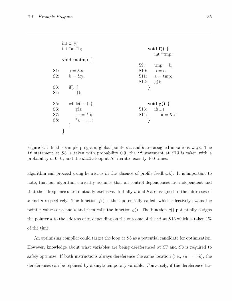
3.1. Example Program 35
int x, y;int *a, *b;
void main() {
S1: a = &x;S2: b = &y;
S3: if(...)S4: f();
S5: while(. . . ) {S6: g();S7: . . . = *b;S8: *a = . . . ;
}}
void f() {int *tmp;
S9: tmp = b;S10: b = a;S11: a = tmp;S12: g();
}
void g() {S13: if(...)S14: a = &x;
}
Figure 3.1: In this sample program, global pointers a and b are assigned in various ways. Theif statement at S3 is taken with probability 0.9, the if statement at S13 is taken with aprobability of 0.01, and the while loop at S5 iterates exactly 100 times.
algorithm can proceed using heuristics in the absence of profile feedback). It is important to
note, that our algorithm currently assumes that all control dependences are independent and
that their frequencies are mutually exclusive. Initially a and b are assigned to the addresses of
x and y respectively. The function f() is then potentially called, which effectively swaps the
pointer values of a and b and then calls the function g(). The function g() potentially assigns
the pointer a to the address of x, depending on the outcome of the if at S13 which is taken 1%
of the time.
An optimizing compiler could target the loop at S5 as a potential candidate for optimization.
However, knowledge about what variables are being dereferenced at S7 and S8 is required to
safely optimize. If both instructions always dereference the same location (i.e., ∗a == ∗b), the
dereferences can be replaced by a single temporary variable. Conversely, if the dereference tar-

3.2. Algorithm Overview 36
gets are always different and also loop invariant then the corresponding dereference operations
can be hoisted out of the loop. If the compiler cannot prove either case to be true, which is
often the result in practice because of the difficulties associated with pointer analysis, then it
must be conservative and halt any attempted optimization. In this particular example, neither
optimization is possible. However, it would be possible to perform either optimization specu-
latively, so long as the optimized code was guarded with a check and recovery mechanism [52].
To decide whether a speculative optimization is desirable, we require the probabilities for the
various points-to relations at S7 and S8.
3.2 Algorithm Overview
The main objective of our probabilistic pointer analysis is to compute, at every program point s
the probability that any pointer α points to any addressable memory location β. More precisely,
given every possible points-to relation 〈α, ∗β〉, the analysis is able to solve for the probability
function ρ(s, 〈α, ∗β〉) for all program points s. The expected probability is defined by the
following equation
ρ(s, 〈α, ∗β〉) =E(s, 〈α, ∗β〉)
E(s)(3.1)
where E(s) is the expected runtime execution frequency associated with program point s and
E(s, 〈α, ∗β〉) is the expected frequency for which the points-to relation 〈α, ∗β〉 holds dynamically
at the program point s [13]. Intuitively, the probability is largely determined by the control-flow
path and the procedure calling context to the program point s—hence an approach that is both
control-flow and context sensitive1 will produce the most probabilistically accurate results.
1A context-sensitive pointer analysis distinguishes between the different calling contexts of a procedure, anda control-flow-sensitive pointer analysis takes into account the order in which statements are executed within aprocedure.

3.2. Algorithm Overview 37
(a) Conventional points-to graph. (b) Probabilistic points-to graph
Figure 3.2: This is a points-to graph and the corresponding probabilistic points-to graph as-sociated with the program point after S4 and initially into S5 (PS5) in the example found infigure 3.1. A dotted arrow indicates a maybe points-to relation whereas a solid arrow denotesa definite points-to relation. UND is a special location set used as the sink target for when apointer’s points-to target is undefined.
To perform pointer analysis, we must first construct an abstract representation of address-
able memory called a static memory model. For our PPA algorithm the static memory model is
composed of location sets [78].2 A location set can represent one or more real memory locations,
and can be classified as a pointer, pointer-target, or both. A location set only tracks its approx-
imate size and the approximate number of pointers it represents, allowing us to abstract away
the complexities of aggregate data structures and arrays of pointers. For example, fields within
a C struct can either be merged into one location set, or else treated as separate location sets.
Such options give us the flexibility to explore the accuracy/complexity trade-off space without
modifying the underlying algorithm. We also define a special location set called UND as the sink
target for when a pointer’s points-to target is undefined.
Since a location set can be a pointer, a location set can point to another location set. Such
a relation is called a points-to relation, and the set of all such relations is called a points-to
graph—a directed graph whose vertices represent location sets. Specifically, a directed edge
2Note that our algorithm itself is not necessarily dependent on this location-set-based model.
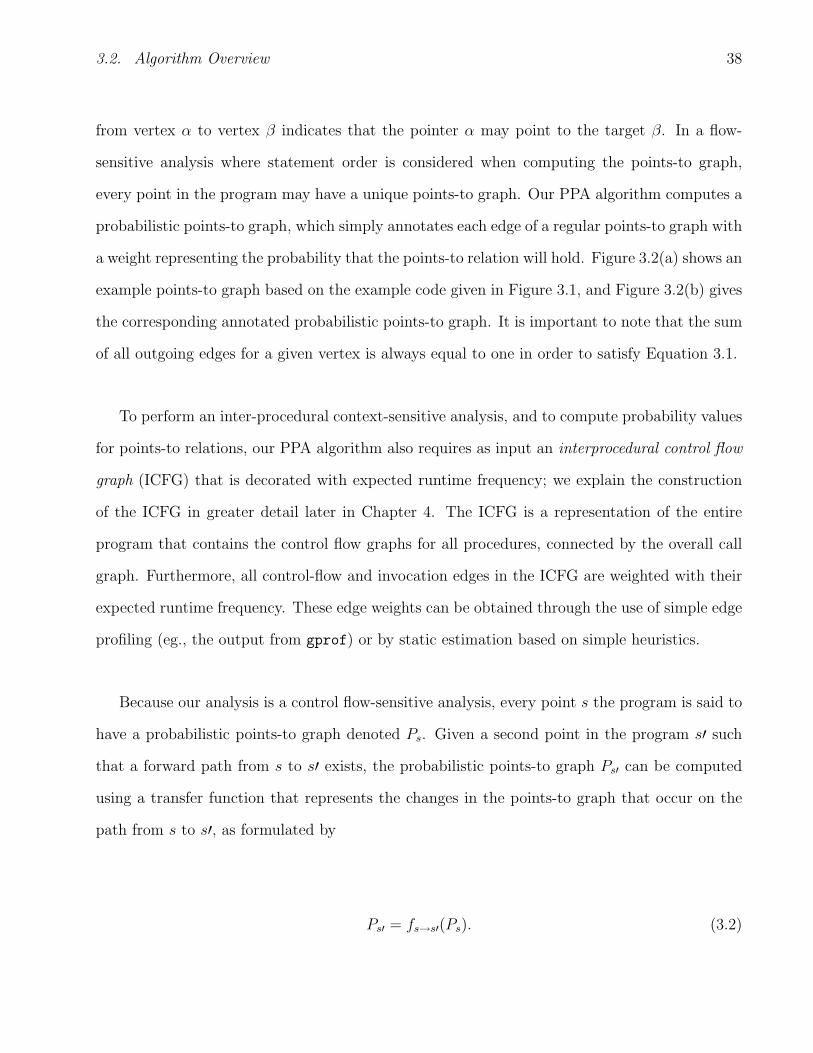
3.2. Algorithm Overview 38
from vertex α to vertex β indicates that the pointer α may point to the target β. In a flow-
sensitive analysis where statement order is considered when computing the points-to graph,
every point in the program may have a unique points-to graph. Our PPA algorithm computes a
probabilistic points-to graph, which simply annotates each edge of a regular points-to graph with
a weight representing the probability that the points-to relation will hold. Figure 3.2(a) shows an
example points-to graph based on the example code given in Figure 3.1, and Figure 3.2(b) gives
the corresponding annotated probabilistic points-to graph. It is important to note that the sum
of all outgoing edges for a given vertex is always equal to one in order to satisfy Equation 3.1.
To perform an inter-procedural context-sensitive analysis, and to compute probability values
for points-to relations, our PPA algorithm also requires as input an interprocedural control flow
graph (ICFG) that is decorated with expected runtime frequency; we explain the construction
of the ICFG in greater detail later in Chapter 4. The ICFG is a representation of the entire
program that contains the control flow graphs for all procedures, connected by the overall call
graph. Furthermore, all control-flow and invocation edges in the ICFG are weighted with their
expected runtime frequency. These edge weights can be obtained through the use of simple edge
profiling (eg., the output from gprof) or by static estimation based on simple heuristics.
Because our analysis is a control flow-sensitive analysis, every point s the program is said to
have a probabilistic points-to graph denoted Ps. Given a second point in the program s′ such
that a forward path from s to s′ exists, the probabilistic points-to graph Ps′ can be computed
using a transfer function that represents the changes in the points-to graph that occur on the
path from s to s′, as formulated by
Ps′ = fs→s′(Ps). (3.2)
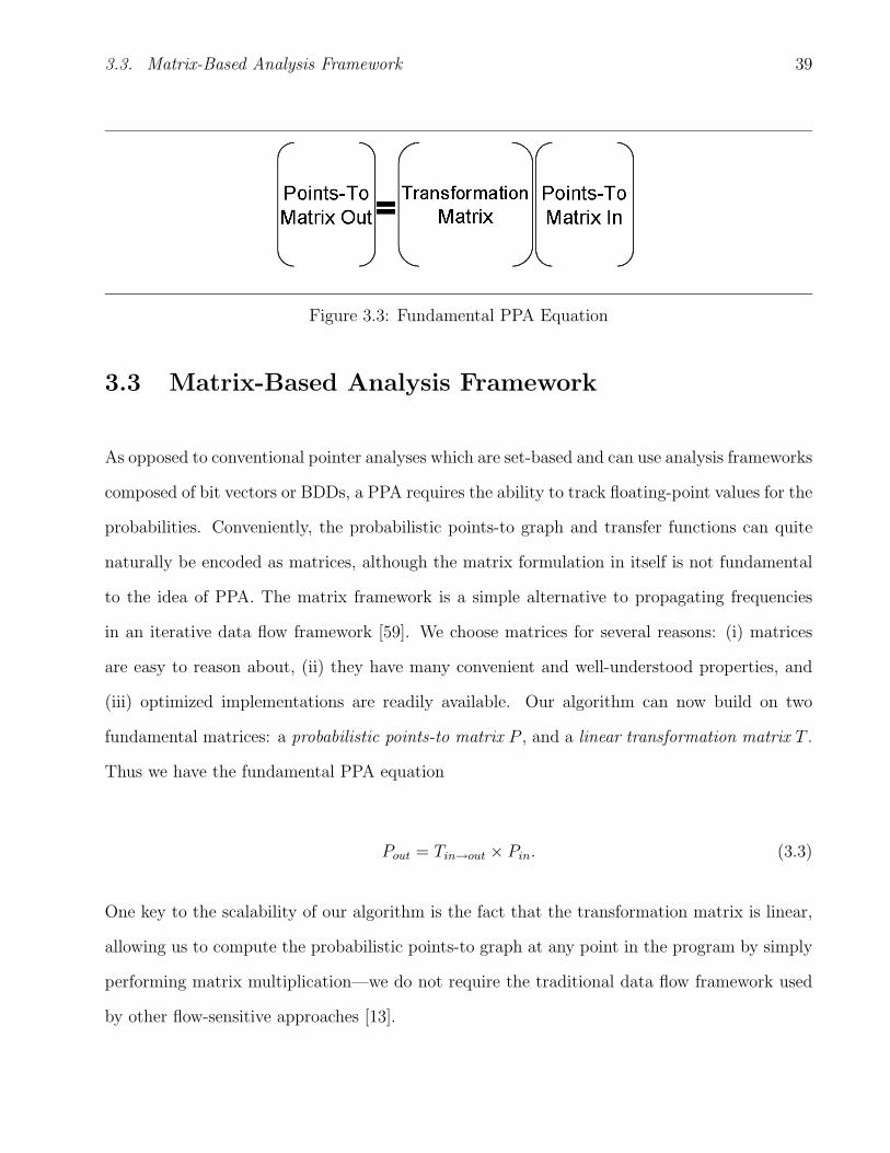
3.3. Matrix-Based Analysis Framework 39
Figure 3.3: Fundamental PPA Equation
3.3 Matrix-Based Analysis Framework
As opposed to conventional pointer analyses which are set-based and can use analysis frameworks
composed of bit vectors or BDDs, a PPA requires the ability to track floating-point values for the
probabilities. Conveniently, the probabilistic points-to graph and transfer functions can quite
naturally be encoded as matrices, although the matrix formulation in itself is not fundamental
to the idea of PPA. The matrix framework is a simple alternative to propagating frequencies
in an iterative data flow framework [59]. We choose matrices for several reasons: (i) matrices
are easy to reason about, (ii) they have many convenient and well-understood properties, and
(iii) optimized implementations are readily available. Our algorithm can now build on two
fundamental matrices: a probabilistic points-to matrix P , and a linear transformation matrix T .
Thus we have the fundamental PPA equation
Pout = Tin→out × Pin. (3.3)
One key to the scalability of our algorithm is the fact that the transformation matrix is linear,
allowing us to compute the probabilistic points-to graph at any point in the program by simply
performing matrix multiplication—we do not require the traditional data flow framework used
by other flow-sensitive approaches [13].

3.3. Matrix-Based Analysis Framework 40
3.3.1 Points-to Matrix
We encode a probabilistic points-to graph using an N × M points-to matrix where M is the
number of location set vertices that can be pointed at, and N is the number of pointer location
sets plus the number of target location sets—therefore the vertices that act both as pointers
and pointee-targets have two matrix row entries and are hence counted twice. The following
equation formally defines the points-to matrix format:
Ps =
p1,1 . . . p1,M
p2,1 . . . p2,M
.... . .
...
pN,1 . . . pN,M
pi,j =
ρ(s, 〈i′, j′〉) i ≤ N − M
1 i > N − M and i = j + (N − M)
0 otherwise
(3.4)
The rows 1 to N−M are reserved for the pointer locations sets and the rows N−M +1 to N
are reserved for the target location sets. To determine the row associated with a given pointer
or pointee variable, the row id(α) function is used. Given a pointer variable α, the function
row id(α) is equal to the matrix row mapped to the pointer α and the function row id(&α) is
equal to the matrix row mapped to the address of α. A pointer with n levels of dereferencing is
additionally mapped to n different rows, one row for each shadow variable represented in every
level the pointer can be dereferenced. For a points-to matrix, pointer-target location sets are
mapped to their corresponding column number by computing row id(&α) − (N − M). The
inner matrix spanning rows 1 to N − M fully describes the probabilistic points-to graph; the
other inner matrix spanning rows N −M +1 to N is the identity matrix, and is only included in

3.3. Matrix-Based Analysis Framework 41
order to satisfy the fundamental PPA equation. Finally, but crucially, the matrix is maintained
such that every row within the matrix sums to one—allowing us to treat a row in the matrix as
a probability vector−→P .
Example Consider the points-to graph depicted in Figure 3.2. We assume that row id(a) = 1,
row id(b) = 2, row id(tmp) = 3, row id(&x) = 4, row id(&y) = 5, and row id(UND) = 6.
We also assume that the columns correspond to x, y, and UND respectively. This produces the
corresponding points-to matrix:
PS5 =
x y UND
a
b
tmp
x
y
UND
0.101 0.899 0
0.9 0.1 0
0 0 1
1 0 0
0 1 0
0 0 1
This points-to matrix indicates that at the program point after S4 and initially into S5 (PS5):
(1) a points to x and y with probabilities 0.101 and 0.899 respectively; (2) b points to x and y
with probabilities 0.9 and 0.1 respectively; and (3) tmp is in an undefined state.
3.3.2 Transformation Matrix
A transfer function for a given points-to matrix is encoded using an N×N transformation matrix,
where N is the number of pointer location sets plus the number of target location sets. Each
row and column is mapped to a specific location set using the equivalent row id(α) function.
Transformation matrices are also maintained such that the values in every row always sum to
one. Given any possible instruction or series of instructions, there exists a transformation matrix
that satisfies Equation 3.3. If a statement has no effect on the probabilistic points-to graph, then

3.4. Representing Assignment Instructions 42
the corresponding transformation matrix is simply the identity matrix. The following sections
describe how transformation matrices are computed.
3.4 Representing Assignment Instructions
In any C program there are four basic ways to assign a value to a pointer, creating a points-to
relation:
1. address assignment: a = &b;
2. pointer assignment: a = b;
3. load assignment: a = ∗b;
4. store assignment: ∗a = b.
For each of the four cases there exists a corresponding transformation matrix. Types (1) and (2)
generate a safe transformation matrix, whereas types (3) and (4) are modeled using a one-level
unsafe transformation. The dereferenced target that is introduced in type (3) or (4) is modeled
as a shadow variable and any ensuing shadow variable aliasing is ignored (for now), which is of
course unsafe. Since speculative optimizations do not necessitate safety we exploit the safety
requirement when multi-level pointer assignment instructions are encountered. Safety can be
added, if it is a requirement, by using some other lightweight alias analysis (this will be discussed
further in Section 3.8). For each of the four cases, a transformation matrix is computed using
the following equation:

3.4. Representing Assignment Instructions 43
T[α=β,p] =
t1,1 t1,2 . . . t1,N
t2,1 t2,2 . . . t2,N
......
. . ....
tN,1 tN,2 . . . tN,N
ti,j =
p i = row id(α) and j = row id(β)
1 − p i = j = row id(α)
1 i = j and i 6= row id(α)
0 otherwise
(3.5)
In this equation, α represents the pointer location set on the left side of the assignment and β
denotes the location set (pointer or target) on the right side of the assignment. The probability
value p represents the binding probability for the transformation and it is equal to 1 divided
by the approximate number of pointers represented by the pointer location set α as defined
in Equation 3.6. A pointer location set can represent multiple pointers. Such a location is
required to represent the following cases: (1) an array of pointers; (2) pointers within recursive
data structures are statically modeled as a single location set; (3) pointers within C structs
are merged when a field-insensitive approach is utilized; and (4) shadow variable aliasing (as
described in Section 3.8). A heuristic is used to approximate how many pointers are represented
by a given pointer location set if this information can not be determined statically. A probability
of p = 1 is equivalent to a strong update used in a traditional flow-sensitive pointer analysis,
where as a probability of p < 1 is representative of a weak update.

3.4. Representing Assignment Instructions 44
p =1
approx # of pointers in α(3.6)
It is important to note that the transformation matrix used for pointer assignment instructions
is simply the identity matrix, with the exception of one row that represents the left side of the
assignment.
Example The transformation matrices corresponding to the pointer assignment statements S1
and S10 from Figure 3.1 are:
TS1 = T[a=&x,1.0] =
0 0 0 1 0 0
0 1 0 0 0 0
0 0 1 0 0 0
0 0 0 1 0 0
0 0 0 0 1 0
0 0 0 0 0 1
TS10 = T[b=a,1.0] =
1 0 0 0 0 0
1 0 0 0 0 0
0 0 1 0 0 0
0 0 0 1 0 0
0 0 0 0 1 0
0 0 0 0 0 1
To compute the points-to matrix at S2 we use TS1 and the fundamental PPA equation as follows:
PS2 = TS1 · PS1
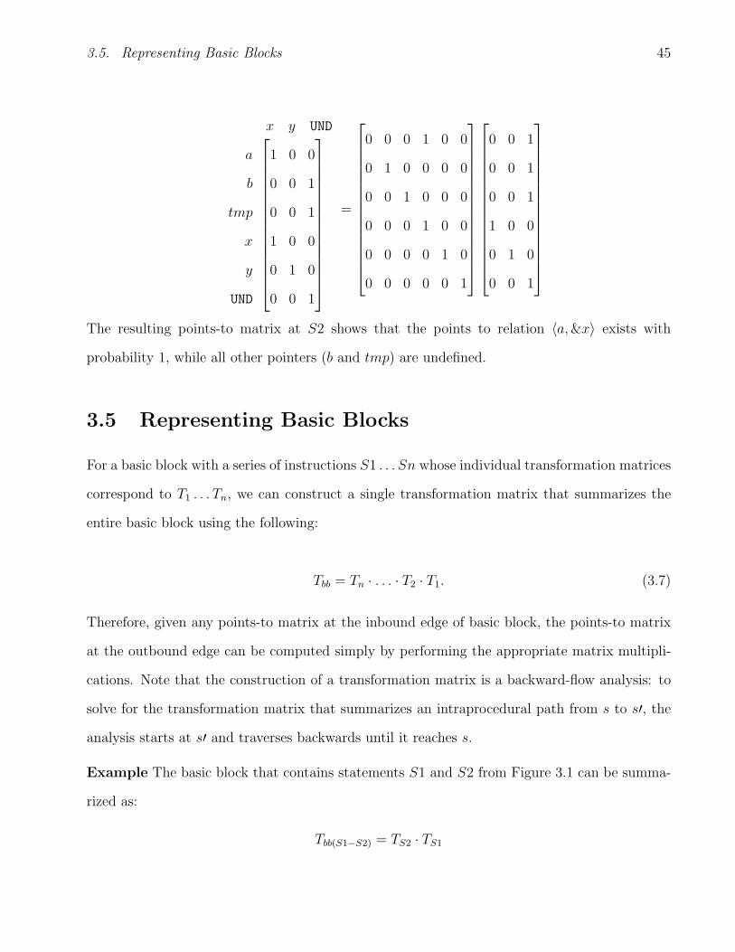
3.5. Representing Basic Blocks 45
x y UND
a
b
tmp
x
y
UND
1 0 0
0 0 1
0 0 1
1 0 0
0 1 0
0 0 1
=
0 0 0 1 0 0
0 1 0 0 0 0
0 0 1 0 0 0
0 0 0 1 0 0
0 0 0 0 1 0
0 0 0 0 0 1
0 0 1
0 0 1
0 0 1
1 0 0
0 1 0
0 0 1
The resulting points-to matrix at S2 shows that the points to relation 〈a, &x〉 exists with
probability 1, while all other pointers (b and tmp) are undefined.
3.5 Representing Basic Blocks
For a basic block with a series of instructions S1 . . . Sn whose individual transformation matrices
correspond to T1 . . . Tn, we can construct a single transformation matrix that summarizes the
entire basic block using the following:
Tbb = Tn · . . . · T2 · T1. (3.7)
Therefore, given any points-to matrix at the inbound edge of basic block, the points-to matrix
at the outbound edge can be computed simply by performing the appropriate matrix multipli-
cations. Note that the construction of a transformation matrix is a backward-flow analysis: to
solve for the transformation matrix that summarizes an intraprocedural path from s to s′, the
analysis starts at s′ and traverses backwards until it reaches s.
Example The basic block that contains statements S1 and S2 from Figure 3.1 can be summa-
rized as:
Tbb(S1−S2) = TS2 · TS1

3.6. Representing Control Flow 46
0 0 0 1 0 0
0 0 0 0 1 0
0 0 1 0 0 0
0 0 0 1 0 0
0 0 0 0 1 0
0 0 0 0 0 1
=
1 0 0 0 0 0
0 0 0 0 1 0
0 0 1 0 0 0
0 0 0 1 0 0
0 0 0 0 1 0
0 0 0 0 0 1
0 0 0 1 0 0
0 1 0 0 0 0
0 0 1 0 0 0
0 0 0 1 0 0
0 0 0 0 1 0
0 0 0 0 0 1
Assume that we are given the points-to matrix for the start of the basic block at S1 in
Figure 3.1; also assume that all pointers are undefined at that point. The points-to matrix at
the end of the basic block (i.e., at S3) can be computed as follows:
PS3 = Tbb(S1−S2) · PS1 =
x y UND
a
b
tmp
x
y
UND
1 0 0
0 1 0
0 0 1
1 0 0
0 1 0
0 0 1
The resulting points-to matrix indicates that at S3 the points-to relations 〈a, &x〉 and 〈b, &y〉
exist with a probability of 1.
3.6 Representing Control Flow
The main objective of this matrix-based PPA framework is to summarize large regions of code
using a single transformation matrix. To summarize beyond a single basic block, our trans-
formation matrices must be able to represent control flow. Recall that the construction of a

3.6. Representing Control Flow 47
(a) Forward edge (b) Back-edge, outside (c) Back-edge, inside
Figure 3.4: Control flow possibilities
transformation matrix proceeds backwards, from s′ backwards to s. When the start of a ba-
sic block is encountered during this backwards analysis, the analysis must categorize the basic
block’s incoming edges. For now we consider the following three non-trivial cases for each edge:
1. the edge is a forward edge (Figure 3.4(a));
2. the edge is a back-edge and s′ is outside the region that the back-edge spans (Figure 3.4(b));
3. the edge is a back-edge and s′ is within the region that the back-edge spans (Figure 3.4(c)).
The following considers each case in greater detail.
3.6.1 Forward Edges
When there exists a single incoming forward edge from another basic block the transformation
matrix that results is simply the product of the current basic blocks transformation matrix
and the incoming blocks transformation matrix. When there are exactly two incoming, forward
edges from basic blocks γ and δ, we compute the transformation matrix as follows:
Tif/else = p · Tγ + q · Tδ (3.8)

3.6. Representing Control Flow 48
Tγ and Tδ represent the transformation matrices from the program point s to the end of each
basic block γ and δ respectively. The scalar probability p represents the fan-in probability from
basic block γ, and q represents the fan-in probability from basic block δ. It is required that p
and q sum to 1. This situation of two forward incoming edges typically arises from the use of
if/else statements. In this case we compute the transformation matrix as follows:
Tcond = pi
∑
Ti (3.9)
This equation is simply a generalized version of Equation 3.8 with the added constraint that
∑
pi = 1.
Example From Figure 3.1 the function g() can be fully summarized using Equation 3.9:
Tg() = 0.01 · TS14 + 0.99 · I =
0.99 0 0 0.01 0 0
0 1 0 0 0 0
0 0 1 0 0 0
0 0 0 1 0 0
0 0 0 0 1 0
0 0 0 0 0 1
The identity matrix I is weighted with a probability 0.99 since there is no else condition.
Recall that the if statement at S13 executes 1% of the time. This matrix indicates that after
the function g() executes, a has 1% chance of pointing at x and 99% chance of remaining the
same.
3.6.2 Back-Edge with s′ Outside it’s Region
When a back-edge is encountered and s′ is outside the region that the back-edge spans, we
can think of the desired transformation matrix as similar to that for a fully-unrolled version

3.6. Representing Control Flow 49
of the loop—eg., the same transformation matrix multiplied with itself as many times as the
trip-count for the loop. In the case where the loop trip-count is constant, we can model the
back-edge through simple exponentiation of the transformation matrix. Assuming that Tx is
the transformation matrix of the loop body, and C is the constant loop trip-count value, we can
model this type of back-edge with the following:
Tloop = TxC (3.10)
When the loop trip-count is not a constant, we estimate the transformation matrix by com-
puting the distributed average of all possible unrollings for the loop. Assuming that the back-
edge is annotated with a lower-bound trip-count value of L and an upper-bound value of U , the
desired transformation matrix can be computed efficiently as the geometric series averaged from
L to U :
Tloop =1
U − L + 1
U∑
L
Txi (3.11)
Example Consider the while loop found at statement S5 in Figure 3.1. The transformation
matrix for the path from S5 to S8 is:
TS5→S8 = (TS6→S8)100 = (Tg())
100 =
0.37 0 0 0.63 0 0
0 1 0 0 0 0
0 0 1 0 0 0
0 0 0 1 0 0
0 0 0 0 1 0
0 0 0 0 0 1
This matrix indicates that after the loop fully iterates, a has a 63% chance of pointing at x and
a 37% chance of remaining unchanged.

3.7. Bottom Up and Top Down Analyses 50
3.6.3 Back-Edge with s′ Inside it’s Region
The final case occurs when the edge is a back-edge and s′ is inside the region that the back-
edge spans, as shown in Figure 3.4(c). Since s′ is within the loop the points-to relations at s′
may change for each iteration of that loop. In this case we compute the desired transformation
matrix using a geometric series such that U is the maximum trip-count value:
Tloop =1
U
U−1∑
0
Txi (3.12)
Example In Figure 3.1 this scenario occurs if we require the transformation matrix for the
path S1 to S7, since in this case s′ is S7, which is within the while loop at S5. The required
transformation matrix can be computed as follows:
TS1→S7 = Tg() · 1100
∑990 (TS6→S8)
i · TS1→S5
3.7 Bottom Up and Top Down Analyses
We have so far described a method for computing probabilistic points-to information across
basic blocks, and hence within a procedure. To achieve an accurate program analysis we need a
method for propagating a points-to matrix inter-procedurally. To ensure that our analysis can
scale to large programs, we have designed a method for inter-procedural propagation such that
each procedure is visited no more than a constant number of times.
We begin by computing a transformation matrix for every procedure through a reverse
topological traversal of the call graph—eg., a bottom-up (BU) pass. Recursive edges in the
call-graph are weakened and analyzed iteratively to ensure that an accurate transformation
matrix is computed. The result of the bottom-up pass is a linear transformation matrix that
probabilistically summarizes the behavior of each procedure.

3.7. Bottom Up and Top Down Analyses 51
In the second phase of the analysis, we initialize a points-to matrix by (i) computing the
result of all statically defined pointer assignments, and (ii) setting all other pointers to point
at the undefined location set (UND). We then propagate the points-to matrix throughout the
entire program using a forward topological traversal of the call-graph (eg., a top-down (TD)
pass). When a load or store instruction is reached, the probability vector for that dereference
is retrieved from the appropriate row in the matrix. When a call instruction is reached we
store the points-to matrix at that point for future use. Finally, we compute the initial points-to
matrix into every procedure as the weighted average of all incoming points-to matrices that were
previously stored.
Example The call graph for our example dictates that in the bottom-up phase of the analysis
the procedure-level transformation matrices are computed in the following order: Tg(), Tf(), and
then Tmain(). This is intuitively necessary since Tf() requires Tg(); and Tmain() requires both Tf()
and Tg(). The algorithm then proceeds into the top-down phase which visits the procedures in
the reverse order. Initially, the following input points-to matrix into main() is used since there
are no static declarations:
Pmain() in =
x y UND
a
b
tmp
x
y
UND
0 0 1
0 0 1
0 0 1
1 0 0
0 1 0
0 0 1
The algorithm propagates and updates this matrix forward until a pointer dereference or a
procedure call instruction is reached. At S4, the points-to matrix PS4 is cached so that when
the procedure f() is analyzed the points-to matrix representing the initial state of f() will be

3.8. Safety 52
available.
Pf() in = PS4 =
x y UND
a
b
tmp
x
y
UND
1 0 0
0 1 0
0 0 1
1 0 0
0 1 0
0 0 1
Similarly, the points-to matrices PS6 and PS12 are also stored in order to analyze procedure g()
during the top-down phase. These matrices are later merged using a weighted sum based on
the fan-in frequencies from their respective callee procedures:
Pg() in = 100 × PS6 + PS12
3.8 Safety
At this point our algorithm does not necessarily compute a safe result in all circumstances:
for certain code, the theoretical points-to transfer function may contain non-linear side effects
which are not captured by our linear transformation matrix encoding. Non-linear effects occur
when multiple levels of dereferencing are used to assign to pointers: (i) load assignment: a = ∗b;
(ii) store assignment: ∗a = b. We optionally handle multi-level dereferencing by instantiating
shadow variable pointer location sets, a technique that is similar to invisible variables [26]. These
shadow variable location sets can potentially alias with other pointer location sets and cause
unsafe behavior if ignored. In this case we want to handle these nonlinearities safely, we use
a lightweight, context-insensitive and flow insensitive unification based alias analysis [65] to
precompute any shadow variable aliasing that can potentially occur. We assume that aliasing
3.9. Summary 53
between location sets occurs with a probability that is inversely-proportionally to the size of
the aliasing set. All transformations involving shadow variables that alias are amended safely
to handle these nonlinearities. However, it is important to note that since we are supporting
speculative optimizations, we also have the option of ignoring safety.
3.9 Summary
This chapter describes the PPA algorithm that provides the foundation for our LOLIPoP infras-
tructure. The points-to matrix and the transformation matrix were introduced as components
used to track and store probabilistic points-to graphs. A simple example was used to show
how transformation matrices can be derived and used to summarize a single instruction, a basic
block, any path, and an entire procedure. A method for leveraging our matrix-based framework
inter-procedurally using a bottom-up and top-down flow was also described. Additionally, a
simple method that utilized a FICI pointer analysis for multiple levels of pointer dereferences
was described as a means of obtaining a safe analysis. The next chapter will describe our design
decisions in greater detail and present the details of our implementation of LOLIPoP.

Chapter 4
The LOLIPoP PPA Infrastructure
This chapter presents the Linear One-Level Interprocedural Probabilistic Pointer (LOLIPoP)
analysis infrastructure. We begin by highlighting and discussing the features that the infras-
tructure offers. The design decisions made and important implementation details to realize this
infrastructure are also discussed in this chapter.
4.1 Implementing LOLIPoP
Figure 4.1 shows a block diagram of the LOLIPoP infrastructure, which operates on C source
code. The LOLIPoP infrastructure is our prototype implementation of the algorithm described
in Chapter 3. The foundation of LOLIPoP is a SUIF 1.3 compiler pass [74]. The SUIF front
end parses the code into the SUIF intermediate representation (SUIF-IR). Using the generated
SUIF-IR, LOLIPoP executes in four sequential phases:
1. Interprocedural Control Flow Graph (ICFG) construction;
2. Static Memory Model (SMM) generation;
3. Bottom-Up (BU) call graph traversal to collect all the procedure-level transformation
54
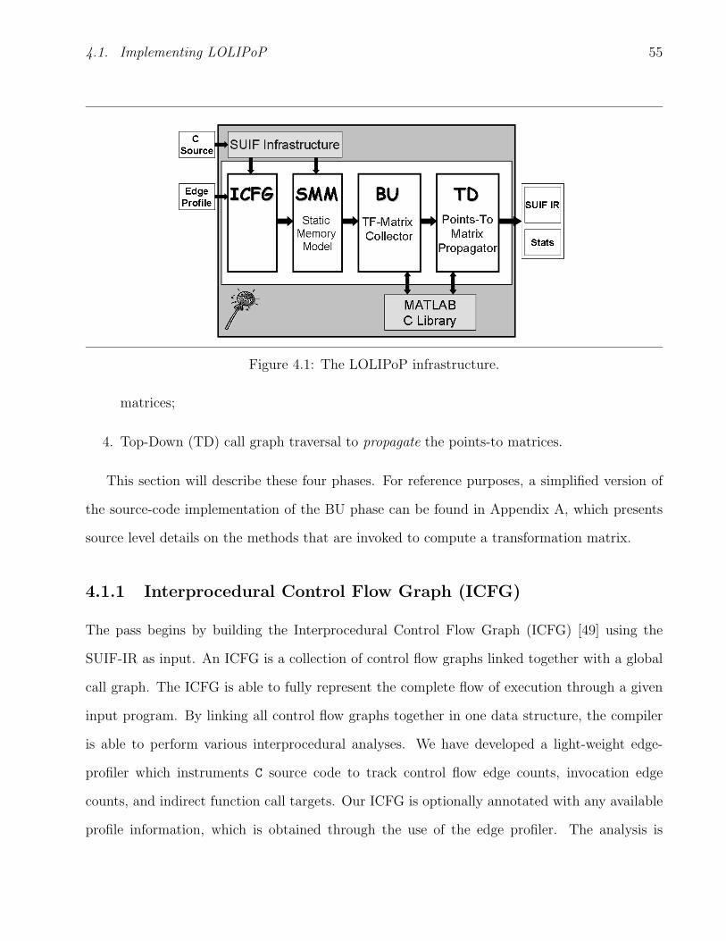
4.1. Implementing LOLIPoP 55
Figure 4.1: The LOLIPoP infrastructure.
matrices;
4. Top-Down (TD) call graph traversal to propagate the points-to matrices.
This section will describe these four phases. For reference purposes, a simplified version of
the source-code implementation of the BU phase can be found in Appendix A, which presents
source level details on the methods that are invoked to compute a transformation matrix.
4.1.1 Interprocedural Control Flow Graph (ICFG)
The pass begins by building the Interprocedural Control Flow Graph (ICFG) [49] using the
SUIF-IR as input. An ICFG is a collection of control flow graphs linked together with a global
call graph. The ICFG is able to fully represent the complete flow of execution through a given
input program. By linking all control flow graphs together in one data structure, the compiler
is able to perform various interprocedural analyses. We have developed a light-weight edge-
profiler which instruments C source code to track control flow edge counts, invocation edge
counts, and indirect function call targets. Our ICFG is optionally annotated with any available
profile information, which is obtained through the use of the edge profiler. The analysis is

4.1. Implementing LOLIPoP 56
optionally able to operate without this profile information through the use of simple static
heuristics, which is discussed further in Section 4.1.5. The ICFG provides a convenient API
so that subsequent phases can easily query for information or traverse the embedded graphs
in various ways. The most important type of traversal predominantly utilized by the BU and
TD phases is a topological traversal of the call graph. However, as a result of recursion, call
graphs may have cyclic components. This prevents us from performing a topological traversal in
the general sense because a topological sorting algorithm requires a directed acyclic call graph.
Therefore, we must somehow remove all cycles. We accomplish this using edge weakening.
Weakening means that we iteratively tag edges within SCCs [72] as ‘weakened’ and then ignore
them during the topological traversal. The implication is that a weakened edge is a recursion-
causing invocation edge.
4.1.2 Static Memory Model (SMM)
After building our ICFG, the next step is to build the static memory model (SMM). The
SMM uses the SUIF symbol table and the ICFG to construct an abstract representation of the
program’s addressable memory space. LOLIPoP uses location sets [78] as defined in Chapter 2 to
abstractly model real memory locations. For our purposes, as described in Chapter 3, a location
set need only track its approximate size and the approximate number of pointers it represents.
Through a linear pass of the SUIF symbol table and ICFG, location sets are extracted, merged,
and represented based on various settings specified by the user. For example, the user is able
to specify how the heap is to be managed: (1) as a single location set, or (2) as a unique
location set that maps every call of malloc(), calloc(), realloc(), etc. to its own location
set. All aggregate structures and arrays are optionally merged into a single location set for a
field-insensitive analysis. This system also allows for a field-sensitive analysis that separates C
struct fields into individual location sets. Recursive data structures are merged into one data

4.1. Implementing LOLIPoP 57
structure after one level of recursion. If necessary, the SMM is responsible for performing a
shadow variable alias analysis pass to guarantee an overall safe analysis. LOLIPoP currently
uses Steensguard’s [65] unification based CIFI alias analysis to extract this alias information.
The various optional user level settings that our SMM provides allow for a fair comparison with
other pointer analysis techniques. They also permit us to further study the various tradeoffs
between efficiency and accuracy.
4.1.3 Bottom-up (BU) Pass
Phase three of our analysis is the bottom-up (BU) pass. The bottom-up pass, as described in
Section 3.7, computes a probabilistic summarizing transformation matrix for every procedure
through a reverse topological traversal of the call graph. We exploit the sparse matrix library
available through MATLAB’s runtime library to perform all matrix operations. The matrices
are cached in an indexable data structure that intelligently monitors its memory usage. If
memory becomes scarce, this storage data structure swaps matrices to disk using traditional
caching algorithms.
At the intraprocedural level, the key method required for the BU phase of the analysis is the
method to compute a transformation matrix given any valid intraprocedural path. This method
fully encapsulates the intraprocedural algorithm described in Chapter 3. The source code can
be found in Section A.4 of Appendix A. This recursive method takes in any two connected
basic blocks and returns the transformation matrix that summarizes the path between those
two basic blocks. Quite naturally, this recursive method is used to compute the transformation
matrix for an entire procedure by passing in the initial and final basic blocks associated with that
procedure1. An important optimization added to the implementation of the algorithm previously
described in Chapter 3 is the use of memoization. To avoid duplicate path computations when
1The ICFG normalizes all control flow graphs so that they have exactly one initial and one final syntheticbasic block [56].
4.1. Implementing LOLIPoP 58
recursively analyzing the same control flow graph, transformation matrices are hashed into a
global table using the path as the hashing index. Because this algorithm is recursive, this
optimization is required to prevent an exponential evaluation of all paths which helps to achieve
scalability.
A further and essential optimization that enables both increased performance and accuracy is
UND-termination. UND-termination sets all local variables, parameters, and return value location
sets to point at UND (the undefined location set) when they can no longer be referenced—
i.e. when they are popped off the program stack. This optimization is completely safe since
location sets local to a procedure no longer point to valid memory locations once the procedure
returns. Although this subtle optimization appears to be inconsequential, its main objective is to
maintain matrix sparsity when calculating other transformation matrices. Without it, matrices
quickly become non-sparse which causes the amount of memory required to grow exponentially.
An example program that has been refactored using UND-termination can be found in Figure 4.2.
4.1.4 Top-down (TD) Pass
The fourth and final stage of the analysis is the top-down (TD) phase. In this phase we visit
every procedure in a forward topological traversal of the call graph. MATLAB’s sparse matrix
runtime library is again utilized to perform all the basic matrix mathematical operations. At
the entry point to every procedure being analyzed we initialize an input points-to matrix. As
described in Section 3.7, this matrix is the weighted sum of all points-to matrices that exist
when this procedure is called. If a procedure has no callee’s, such as the main() procedure, we
initialize an input points-to matrix by (i) computing the result of all statically defined pointer
assignments, and (ii) setting all other pointers to point at the undefined location set (UND).
At the intraprocedural level, the points-to matrix is also propagated in a top-down traversal
of the control flow graph using an equivalent traversal algorithm as the one used at the inter-
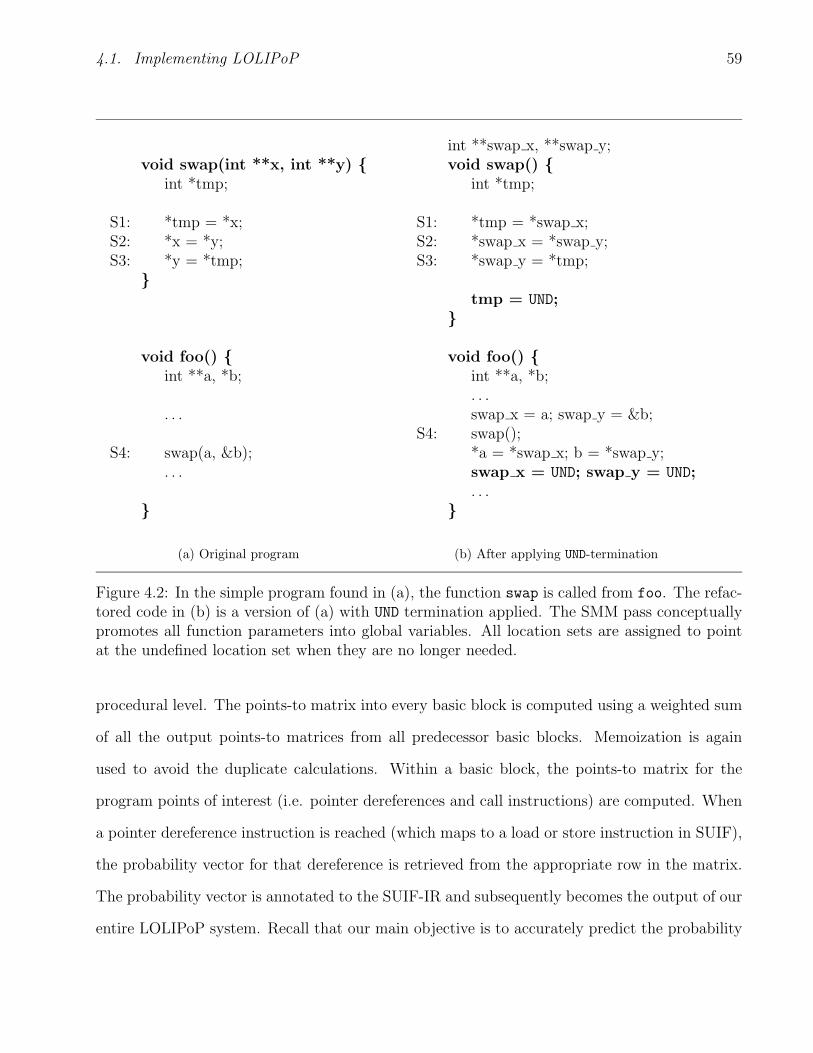
4.1. Implementing LOLIPoP 59
void swap(int **x, int **y) {int *tmp;
S1: *tmp = *x;S2: *x = *y;S3: *y = *tmp;
}
void foo() {int **a, *b;
. . .
S4: swap(a, &b);. . .
}
(a) Original program
int **swap x, **swap y;void swap() {
int *tmp;
S1: *tmp = *swap x;S2: *swap x = *swap y;S3: *swap y = *tmp;
tmp = UND;}
void foo() {int **a, *b;. . .swap x = a; swap y = &b;
S4: swap();*a = *swap x; b = *swap y;swap x = UND; swap y = UND;. . .
}
(b) After applying UND-termination
Figure 4.2: In the simple program found in (a), the function swap is called from foo. The refac-tored code in (b) is a version of (a) with UND termination applied. The SMM pass conceptuallypromotes all function parameters into global variables. All location sets are assigned to pointat the undefined location set when they are no longer needed.
procedural level. The points-to matrix into every basic block is computed using a weighted sum
of all the output points-to matrices from all predecessor basic blocks. Memoization is again
used to avoid the duplicate calculations. Within a basic block, the points-to matrix for the
program points of interest (i.e. pointer dereferences and call instructions) are computed. When
a pointer dereference instruction is reached (which maps to a load or store instruction in SUIF),
the probability vector for that dereference is retrieved from the appropriate row in the matrix.
The probability vector is annotated to the SUIF-IR and subsequently becomes the output of our
entire LOLIPoP system. Recall that our main objective is to accurately predict the probability

4.1. Implementing LOLIPoP 60
of each points-to relation at every pointer dereference program point. When a call instruction
is reached we store the points-to matrix at that point for future use. The data structure that
stores these matrices performs the interprocedural merge operation immediately to reduce the
total number of matrices required for storage.
4.1.5 Heuristics
To a large extent, the probabilistic points-to information extracted at every pointer dereference
point is dependent on the edge-profile information used to guide the analysis—the assumption
being that the degree of accuracy used in obtaining edge profile information is directly related to
the final probabilistic accuracy. The exact impact of an accurate edge-profile pass was unclear
at the outset of our investigation and the actual measured impact will be discussed later in
Chapter 5. Our analysis requires four different types of information from the edge profiler: (i)
the fan-in probability of all control flow graph edges (ignoring back edges); (ii) the upper and
lower bound trip counts for all back edges per loop invocation; (iii) the fan-in probability of
all invocation call graph edges; and (iv) the probability of indirect function call targets. For
experiments when edge-profile information is not available, simple heuristics are used in its place.
The following three compile-time heuristics are used: (i) we assume that fan-in probability is a
uniform distribution between all incoming branches; (ii) when the upper and lower bound for the
trip count of a loop cannot be determined through a simple inspection of the loop bounds, we
assume that the lower bound is zero and the upper bound is ten; and (iii) we assume that fan-in
call graph invocation edge counts have a uniform distribution between all callee procedures. For
this thesis we do not yet use a heuristic for indirect function call targets and therefore require
the edge-profiler to always provide that information.

4.2. Accuracy-Efficiency Tradeoffs 61
4.2 Accuracy-Efficiency Tradeoffs
During the design and implementation of LOLIPoP, many important design decisions involving
accuracy/efficiency tradeoffs were encountered. Many of these tradeoffs are common to all
pointer analysis algorithms, as discussed in Section 2.1.6. Our system was designed so that
whenever possible, and especially when no approach was clearly favourable, the trade-off was
left for the eventual client of LOLIPoP to control. This section will briefly discuss some of the
important tradeoffs encountered and the approach taken.
4.2.1 Safe vs Unsafe Analysis
Because our analysis targets a speculative client optimization, safety is not a firm requirement.
That said, safety can potentially aid a speculative optimization by reducing the number of
memory references which must be treated as speculative. For example, reordering loads and
stores using the EPIC instruction set requires the memory references to always be speculative
instructions if an unsafe analysis is used. In contrast, if a safe analysis is used the compiler would
be able to, in certain cases, guarantee that an optimization is safe and could avoid the overhead
that results from tracking speculative loads and stores. Clearly a tradeoff exists here between
accuracy and efficiency. Performing a safe analysis adds complexity and increases the run time of
our algorithm for three reasons: (i) the added time required to perform the shadow variable alias
analysis pass; (ii) the increased complexity in deriving and computing transformation matrices
that represent instructions where an operand aliases with another location set; and (iii) the
decrease in matrix sparsity as a consequence of adding and tracking many likely false points-to
relations. For the reasons described here, LOLIPoP was designed to allow the user to optionally
decide if a safe or unsafe analysis should be performed.
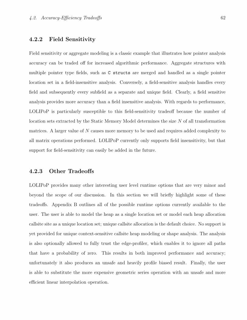
4.2. Accuracy-Efficiency Tradeoffs 62
4.2.2 Field Sensitivity
Field sensitivity or aggregate modeling is a classic example that illustrates how pointer analysis
accuracy can be traded off for increased algorithmic performance. Aggregate structures with
multiple pointer type fields, such as C structs are merged and handled as a single pointer
location set in a field-insensitive analysis. Conversely, a field-sensitive analysis handles every
field and subsequently every subfield as a separate and unique field. Clearly, a field sensitive
analysis provides more accuracy than a field insensitive analysis. With regards to performance,
LOLIPoP is particularly susceptible to this field-sensitivity tradeoff because the number of
location sets extracted by the Static Memory Model determines the size N of all transformation
matrices. A larger value of N causes more memory to be used and requires added complexity to
all matrix operations performed. LOLIPoP currently only supports field insensitivity, but that
support for field-sensitivity can easily be added in the future.
4.2.3 Other Tradeoffs
LOLIPoP provides many other interesting user level runtime options that are very minor and
beyond the scope of our discussion. In this section we will briefly highlight some of these
tradeoffs. Appendix B outlines all of the possible runtime options currently available to the
user. The user is able to model the heap as a single location set or model each heap allocation
callsite site as a unique location set; unique callsite allocation is the default choice. No support is
yet provided for unique context-sensitive callsite heap modeling or shape analysis. The analysis
is also optionally allowed to fully trust the edge-profiler, which enables it to ignore all paths
that have a probability of zero. This results in both improved performance and accuracy;
unfortunately it also produces an unsafe and heavily profile biased result. Finally, the user
is able to substitute the more expensive geometric series operation with an unsafe and more
efficient linear interpolation operation.

4.3. Optimizations 63
4.3 Optimizations
To meet our objective to scale to the entire SPEC 2000 integer benchmark suite, we put a
great deal of effort into optimizing the execution of LOLIPoP. In particular we exploit sparse
matrices, we compress matrices before exponentiating, we perform aggressive memoization of
matrix results at the intraprocedural level, and we use an efficient implementation for computing
the geometric series for Equations 3.11 and 3.12. This section describes the main optimizations
utilized to realize our scalability objective.
4.3.1 Matrix Representation
The typical data structure used for a matrix is a two dimensional array. Each entry in the
array represents an element ai,j of the matrix and can be accessed by the two indices i and
j. For our purposes, the matrices are almost always sparse, and implementing them using this
naive approach is an inefficient use of memory. In this regard, we exploit the fact that our
matrices are sparse and therefore encode them using Matlab’s sparse matrix library [41, 53].
We also take special care, as discussed previously, to ensure that the matrices remain sparse to
effectively take advantage of the Matlab library. A sparse matrix contains many zero entries.
The basic idea when storing sparse matrices is to only store a representation of non-zero entries
as opposed to storing all entries. Depending on the number and distribution of the non-zero
entries, different data structures can be used and yield huge savings in memory when compared
to a naive approach.
Matlab encodes sparse matrices using the Yale Sparse Matrix Format [25, 35]. It stores an
initial sparse N × N matrix M in row form using three arrays: PR, IR, and JC. The variable
NZ denotes the number of nonzero entries in matrix M . PR is an array of type double that
stores all nonzero entries within M . This array is therefore at least length NZ and we ensure
that it does not grow beyond 2 × NZ (surprisingly, Matlab does not maintain this for us).

4.3. Optimizations 64
The array IR is also at least of length NZ. It is an integer array that stores the row offsets
associated with the values in PR. JC is an integer array of length N +1. IR stores at JC[i] the
position of the first element of row i in the sparse array PR. The length of row i is determined
by JC[i + 1] − JC[i].
4.3.2 Matrix Operations
A further optimization we use is matrix compression. The matrices we maintain have the
property that all rows sum to 1.0, which implies that they contain at least N nonzero entries—
therefore, we don’t fully take advantage of the sparsity features provided by Matlab. Whenever
storing transformation matrices, we compress them by subtracting the identity matrix. Since
most transformation matrices are very close to the identity matrix, this causes them to become
much more sparse. They are therefore stored using a more memory efficient means, which
indirectly results in improved performance.
When performing exponentiation or the geometric series operation we utilize a different type
of matrix compression. We compress the matrix into a smaller matrix by eliminating all rows and
columns that will remain unchanged after the operation is performed [16]. We then perform the
exponentiation or geometric series operation on the smaller matrix. The matrix is then repaired
back into its former state by reinserting the rows and columns that were removed. This type of
matrix compression can be performed on the Yale matrix type quite easily and matlab performs
much more efficiently when exponentiating a smaller matrix.
For performing the expensive operation of exponentiation, LOLIPoP relies on the Matlab
library for which it is undocumented how exponentiation is performed efficiently. Furthermore, it
is hypothesized that LOLIPoP could improve upon Matlab’s implementation of exponentiation
by further utilizing the various properties of the transformation matrix—this is left for future
work. The geometric series operation is implemented by LOLIPoP as an extension to the
4.4. Summary 65
exponentiation operation. More information on how to map a geometric series operation into
an exponentiation operation can be found in Appendix C.
4.4 Summary
This chapter presented the LOLIPoP infrastructure. We described the four phases used by
the LOLIPoP framework: (1) Interprocedural Control Flow Graph (ICFG) construction; (2)
Static Memory Model (SMM) generation; (3) Bottom-Up (BU) traversal; and (4) Top-Down
(TD) traversal. We highlighted the features that the infrastructure offers. We discussed the
different tradeoffs involved, including field sensitivity and safe vs unsafe analysis. We also
provided insight into the important implementation details and optimizations that we applied
such as: memoization, UND-termination, and matrix compression. The next chapter will discuss
the experimental framework used and the accuracy and performance results we obtained.

Chapter 5
Evaluating LOLIPoP
In this chapter we evaluate LOLIPoP’s running-time, the accuracy of the pointer analysis results
in a conventional sense, and the accuracy of the resulting probabilities.
5.1 Experimental Framework
The following describes our framework for evaluating LOLIPoP. All timing measurements were
obtained using a 3GHz Pentium IV with 1GB of RAM and 1GB of swap space. We report
results for all of the SPECint95 and SPECint2000 benchmarks [19] except for the following:
252.eon, which is written in C++ and therefore not handled by our compiler; 126.gcc, which
is similar to 176.gcc; and 147.vortex, which is identical to 255.vortex. Table 5.1 describes
both the ref and train inputs used for each benchmark.
5.2 Analysis Running-Time
LOLIPoP meets our objective of scaling to the SPECint95 and SPECint2000 benchmark suites.
Table 5.2 shows the running-times for both the safe (where shadow variable alias analysis is per-
66
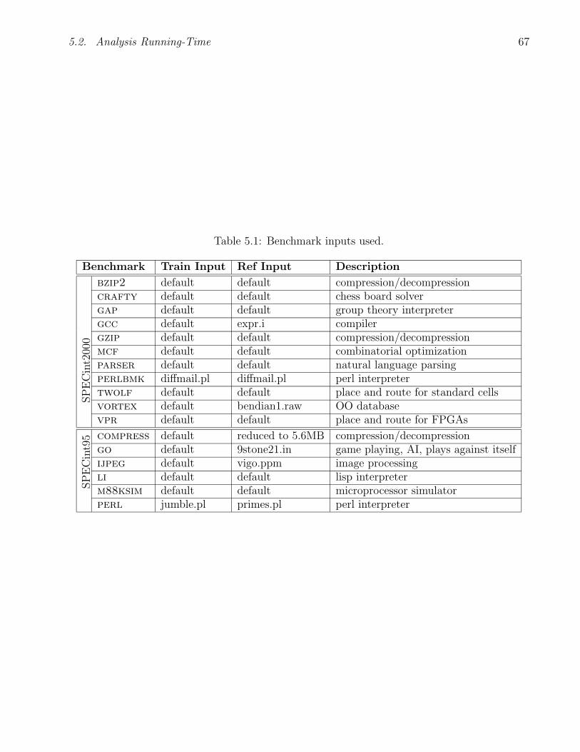
5.2. Analysis Running-Time 67
Table 5.1: Benchmark inputs used.
Benchmark Train Input Ref Input Description
SP
EC
int2
000
bzip2 default default compression/decompressioncrafty default default chess board solvergap default default group theory interpretergcc default expr.i compilergzip default default compression/decompressionmcf default default combinatorial optimizationparser default default natural language parsingperlbmk diffmail.pl diffmail.pl perl interpretertwolf default default place and route for standard cellsvortex default bendian1.raw OO databasevpr default default place and route for FPGAs
SP
EC
int9
5 compress default reduced to 5.6MB compression/decompressiongo default 9stone21.in game playing, AI, plays against itselfijpeg default vigo.ppm image processingli default default lisp interpreterm88ksim default default microprocessor simulatorperl jumble.pl primes.pl perl interpreter

5.2. Analysis Running-Time 68
Table 5.2: LOLIPoP measurements, including lines-of-code (LOC) and transformation matrixsize N for each benchmark, as well as the running times for both the unsafe and safe analyses.The time taken to obtain points-to profile information at runtime is included for comparison.
Matrix Running Time (min:sec)Benchmark LOC Size Unsafe Safe PT-Profile
SP
EC
int2
000
bzip2 4686 251 0:0.3 0:0.3 13:34crafty 21297 1917 0:5.5 0:5.5 14:47gap 71766 25882 54:56 83:38 55:56gcc 22225 42109 309:40 N/A 39:58gzip 8616 563 0:0.71 0:0.77 3:48mcf 2429 354 0:0.39 0:0.61 19:46parser 11402 2732 0:30.7 0:50.0 84:52perlbmk 85221 20922 44:15 89:43 N/Atwolf 20469 2611 0:16.6 0:20.6 N/Avortex 67225 11018 3:59 4:56 0:0.7vpr 17750 1976 0:9.3 0:10.3 197:0
SP
EC
int9
5 compress 1955 97 0:0.1 0:0.1 1:55go 29283 651 0:2.9 0:3 5:58ijpeg 31457 4491 0:23.4 0:24.9 7:12perl 4686 5395 5:3 7:49 8:37li 27144 3868 0:28.8 0:59.15 72:5m88ksim 19933 1932 0:4.9 0:5.24 0:0.2

5.2. Analysis Running-Time 69
formed) and unsafe analyses. Each running-time includes the bottom-up and top-down phases
of the overall analysis, but ignores the time taken to build the interprocedural control flow graph
and static memory model—but note that this time is negligible in most cases. The runtimes
range from less than a second for four benchmarks up to 5 hours for the challenging bench-
mark (gcc). These results are promising especially given that this is an academic prototype
implementation of PPA.
For speculative optimizations, the alternative to pointer analysis is to use a points-to profiler
which instruments the source code to extract points-to frequency information at runtime—for
comparison purposes, we have implemented a points-to profiler. Our points-to profiler instru-
ments the source code so that the memory addresses of all location sets can be tracked and
queried at runtime. This involves two key instrumentation techniques: (1) overloading library
function calls to alloc and free to track heap location set addresses; and (2) storing the
addresses of every stack variable (whose address is taken) when it gets put on the program’s
runtime stack. Every pointer dereference is also instrumented with a wrapper function that
enables the points-to profiler to determine which location set is being referenced during the
dereference operation. The points-to profiler queries the set of available addresses, which takes
O(n · log(n)) time, to determine which runtime point-to relation is executing—the frequency
of this points-to relation is then incremented. Points-to profiling is a computationally intense
analysis and furthermore has no ability to provide safety in the resulting alias information it
provides.
The results in Table 5.2 show that in most cases, our analysis approach is much faster than
the profiler. In fact, for two cases (perlbmk and twolf) the profiler did not terminate after
two weeks of execution. It is also important to note that the profiling approach is very dependent
on the input set used, both in the results it provides and on the profiler’s runtime. For gcc and
vortex reduced reference input sets were used to ensure a tractable profiler time (described in
Table 5.1)—in these cases the profiler outperforms LOLIPoP because LOLIPoP must analyze

5.3. Pointer Analysis Accuracy 70
|0
|50
|100
Ave
rag
e D
eref
. Siz
e
L
1.1
G
1.2
com
pres
sL
2.6
G7.
7
*gcc
L3.
3G
14.8
goL
6.7
G
11.9
ijpeg
L
80.1
*185
.6
Gli
L
1.8
G
3.3
m88
ksim
L
18.5
G
21.9
perl
L
6.1
G
59.3
vorte
x
Figure 5.1: Average dereference size comparison with GOLF for the SPECInt95 benchmarks:L is LOLIPoP, and G is GOLF. LOLIPoP’s results are safe, except for gcc which reports anunsafe result. LOLIPoP’s results are more accurate than GOLF for all benchmarks.
the entire program while the profiler only analyzes the subset of code that is exercised by the
reduced input set. For the more challenging benchmarks (gap, gcc, and perlbmk), there is a
significant increase in running-time to compute safe results—i.e., to handle pointer assignments
with multiple levels of dereferencing as described in Section 3.8.
5.3 Pointer Analysis Accuracy
The accuracy of a conventional pointer analysis algorithm is typically measured and compared
by computing the average cardinality of the target location sets that can be dereferenced across
all pointer dereference sites in the program—in short, the average dereference size. To ensure
that LOLIPoP is indeed accurate, in Figure 5.1 we compare the average dereference size for
LOLIPoP’s safe result with those reported by Das for the GOLF algorithm [22]. We choose
GOLF for comparison for two main reasons: (i) it is one of the few analyses that scales to even
SPECint95 benchmarks; (ii) GOLF is safe, one-level context-sensitive, field-insensitive, and

5.3. Pointer Analysis Accuracy 71
Table 5.3: LOLIPoP Measurements.
Avg. Dereference SizeBenchmark Safe p > 0.001 Unsafe
bzip2 1.00 1.00 1.00compress 1.080 1.08 1.08crafty 1.830 1.40 1.83gap 143.84 77.61 6.21gcc N/A N/A 2.64go 3.290 2.15 3.29gzip 1.41 1.31 1.45ijpeg 6.740 2.46 1.33li 80.10 14.70 4.34m88ksim 1.82 1.66 1.84mcf 1.51 1.51 1.51parser 42.52 2.09 3.23perlbmk 18.48 5.45 3.10perl 88.98 8.40 35.35twolf 1.26 1.25 1.19vortex 6.06 3.61 6.13vpr 1.18 1.10 1.09
callsite-allocating—matching those aspects of LOLIPoP. However, our goal is not to compete
with GOLF since there are several reasons such a comparison would not be fair: (i) LOLIPoP
is flow-sensitive while GOLF is not; (ii) LOLIPoP relies on profiling to identify the targets
of function pointers; and (iii) LOLIPoP does not yet model all library calls, while GOLF does.
Flow-sensitivity is the main reason that LOLIPoP does not scale as well as GOLF, although this
is also the main source of LOLIPoP’s significantly improved accuracy as reported in Figure 5.1.
In summary, even without considering probability information LOLIPoP provides an accurate
approach to performing pointer analysis.
Table 5.3 shows the average dereference sizes for all benchmarks studied, showing the safe
result, the result when any points-to relation with a probability less than 0.001 is ignored, and

5.4. Probabilistic Accuracy 72
the unsafe result (when shadow variable aliasing is ignored)—average maximum certainty will
be discussed later in Section 5.4.1. One very interesting result is that the benchmarks with
a relatively large average dereference size for the safe analysis (gap, li, parser, perlbmk,
perl) show a dramatic decrease when unlikely points-to relations are ignored (i.e., those for
which p < 0.001). This result suggests that many points-to relations are unlikely to occur at
runtime, underlining the strong potential for speculative optimizations. As expected, a similar
result is observed for the unsafe version of the analysis since the safe analysis introduces many
inaccuracies through the flow-insensitive, context-insensitive pass that addresses shadow variable
aliasing. These inaccuracies create many low probability points-to relations that are unlikely to
ever occur at runtime. For example, the safe average dereference size for gap is relatively high
at 143.84, while the unsafe size is only 6.21.
5.4 Probabilistic Accuracy
We now measure the accuracy of the probabilities computed by LOLIPoP by comparing the
two probability vectors−→P s and
−→P d at every pointer dereference point.
−→P s, as defined in
Section 3.3.1, represents the probability vector reported by LOLIPoP—the static probability
vector.−→P d represents the dynamic probability vector calculated by the points-to profiler. In
particular, we want to quantify the accuracy of the probability vectors−→Ps that are statically
computed at every pointer dereference. For comparison, we use the results of the profiler where
each benchmark (using it’s ref input) is instrumented to track—for each pointer dereference
location—a frequency vector that indicates the frequency that each location set is the target.
Each resulting dynamic frequency vector is then normalized into a dynamic probability vector
(−→P d) so that it may be compared with the corresponding probability points-to relation vector,
as described in Equation 3.1. To compare the two vectors in a meaningful way, we compute the
normalized average Euclidean distance (NAED) as defined by:

5.4. Probabilistic Accuracy 73
|0.0
|0.2
|0.4
|0.6
SPE
Cint
95 N
orm
. Ave
rage
Euc
lidea
n Di
st.
D 0.
03
Sr
0.03
Ur
0.03
Ut
0.03
Un
0.03
compress
D 0.
07
Sr
0.03
Ur
0.03
Ut
0.04
Un
0.04
go
D 0.
55
Sr
0.41
Ur
0.43
Ut
0.43
Un
0.53
ijpeg
D 0.
63
Sr
0.64
Ur
0.56
Ut
0.51
Un
0.45
liD
0.39
Sr
0.33
Ur
0.33
Ut
0.36
Un
0.37
m88ksim
D 0.
58
Sr
0.41
Ur
0.31
Ut
0.27
Un
0.33
perl
D 0.
38
Sr
0.31
Ur
0.28
Ut
0.27
Un
0.29
average
Figure 5.2: SPECint95 - Normalized Average Euclidean Distance (NAED) relative to the dy-namic execution on the ref input set. D is a uniform distribution of points-to probabilities, Sr isthe safe LOLIPoP result using the ref input set, and the U bars are the unsafe LOLIPoP resultusing the ref (Ur) and train (Ut) input sets, or instead using compile-time heuristics (Un).
NAED =1√2·
∑ ‖−→P s −−→P d‖
(# pointer dereferences)(5.1)
This metric summarizes the average error uniformly across all probability vectors at every pointer
dereference on a scale that ranges from zero to one, where a zero means no discrepancy between
dynamic and static vectors, and a one means there is always a contradiction at every dereference.
Figures 5.2 and 5.3 show the NAED for the SPECint95 and SPECint2000 benchmarks rela-
tive to the dynamic execution on the ref input set (results for gap, perlbmk, and twolf are
omitted because their dynamic points-to profile information could not be tractably computed).

5.4. Probabilistic Accuracy 74
|0.0
|0.2
|0.4
|0.6
SPE
Cint
2000
Nor
m. A
vera
ge E
uclid
ean
Dist
.
D 0.
00Sr
0.
00Ur
0.
00Ut
0.
00Un
0.
00
bzip2
D 0.
23Sr
0.
01Ur
0.
01Ut
0.
02Un
0.
07
crafty
D 0.
18Sr
0.
12Ur
0.
21Ut
0.
21Un
0.
24
gzip
D 0.
46Sr
0.
46Ur
0.
46Ut
0.
46Un
0.
46
mcf
D 0.
62Sr
0.
57Ur
0.
36Ut
0.
36Un
0.
39
parserD
0.58
Sr
0.41
Ur
0.31
Ut
0.27
Un
0.33
perl
D 0.
49Sr
0.
29Ur
0.
30Ut
0.
30Un
0.
43
vortex
D 0.
26Sr
0.
25Ur
0.
26Ut
0.
26Un
0.
27
vpr
D 0.
32Sr
0.
24Ur
0.
23Ut
0.
23Un
0.
27
average
Figure 5.3: SPECint2000 - Normalized Average Euclidean Distance (NAED) relative to thedynamic execution on the ref input set. D is a uniform distribution of points-to probabilities,Sr is the safe LOLIPoP result using the ref input set, and the U bars are the unsafe LOLIPoPresult using the ref (Ur) and train (Ut) input sets, or instead using compile-time heuristics (Un).
In the first experiment (D) we distribute probability uniformly to every target in the static
points-to probability vector−→Ps, making the naive assumption that all targets are equally likely.
This experiment is used to quantify the value-added of probability information, and leads to an
average NAED across all benchmarks of 0.32 relative to the dynamic result. It is important to
notice that for bzip2, compress, and go even the uniform distribution (D) is quite accurate.
For bzip2 and compress this is an expected result since the average dereference size (shown
in Figure 5.3) is very close to 1.0.
The second experiment (Sr) plots the NAED for the safe analysis using edge-profile in-

5.4. Probabilistic Accuracy 75
formation from the ref input set. Comparing the static and dynamic results using the same
input set allows us to defer the question of how representative the profiling input set is. With
LOLIPoP we improve the NAED to an average of 0.25 across all benchmarks, although that
average can be misleading. For about half of the benchmarks probability information does
not make a large difference (bzip2, compress, go, m88ksim, mcf, vpr), while for the remaining
benchmarks probability information significantly improves the NAED. For li, the probability
information slightly increases the NAED. The li benchmark contains a tremendous amount of
shadow variable aliasing—we know this because of the large gap between the safe and unsafe
average dereference sizes shown in Figure 5.3. The spurious points-to relations introduced by
the ‘safe’ analysis appear to corrupt the useful probability information. A similar result would
be expected for gap. Using a more accurate shadow variable analysis pass would help to reduce
this effect. Also, applying field-sensitivity would also help because it would drastically reduce
the amount of shadow variable aliasing.
The next experiment (Ur) shows the NAED for the unsafe analysis, also using edge-profile
information from the ref input set. Comparing with the safe experiment (Sr), surprisingly we see
that on average the unsafe result is more accurate (with an NAED of 0.24): this result implies
that safety adds many false points-to relations, and can actually be undesirable in the context
of speculative optimizations. The exception to this is gzip, where the NAED deteriorates when
transitioning from safe to unsafe. This implies that gzip frequently utilizes and relies on many
levels of pointer dereferencing.
The final two experiments plot the NAED for the unsafe analysis when using the train
input set (Ut), and when using compile-time heuristics instead of edge-profile information (Un).
Surprisingly, the average NAED when using the train input set (Ut) is slightly more accurate
than with the ref input set (Ur): this indicates that there are aliases which occur rarely during
the ref execution, which when profiled and fed back into LOLIPoP, become a source of inaccuracy
compared to the lesser coverage of the train input set. Finally, we see that the unsafe approaches
5.4. Probabilistic Accuracy 76
are more accurate with edge-profiling information than when compile-time heuristics are used
(Un), although even with the heuristic approach LOLIPoP is more accurate than the uniform
distribution (D).
5.4.1 Average Maximum Certainty
To further evaluate the potential utility of points-to probability information provided by LOLIPoP,
we use a measure average maximum certainty:
Avg. Max. Certainty =
∑
(Max Probability Value)
(# pointer dereferences)(5.2)
This equation takes the maximum probability value associated with all points-to relations
at every pointer dereference and averages these values across all pointer dereference sites. Data
speculative optimizations benefit from increased certainty that a given points-to relation exists:
since the probabilities across a probability vector sum to one, if there is one large probability
it implies that the probabilities for the remaining location sets are small. In other words, the
closer the average maximum certainty value is to one, the more potential there is for successful
speculative optimization. The average maximum certainty for each SPEC benchmark is given
in Table 5.4, and in general these values are quite high: the average value across all benchmarks
is 0.899. This indicates that on average, at any pointer dereference, there is likely only one
dominant points-to relation. Therefore a client analysis using LOLIPoP will be very certain
of which points-to relation will exist at a given pointer dereference. The actual average max
certainty values appear to be directly correlated to the average dereference size. If the average
dereference size is quite high for a given benchmark then it’s max certainty value is relatively
smaller. Intuitively, this is an expected result.

5.4. Probabilistic Accuracy 77
Table 5.4: LOLIPoP Average Maximum Certainty Measurements.
Avg.Maximum
Benchmark Certainty
bzip2 1.00compress 0.96crafty 0.95gap 0.78gcc 0.96go 0.94gzip 0.90ijpeg 0.90li 0.76m88ksim 0.83mcf 0.92parser 0.97perlbmk 0.79perl 0.87twolf 0.90vortex 0.91vpr 0.95Average 0.899

5.5. Summary 78
5.5 Summary
This chapter discussed the experimental framework we used in evaluating LOLIPoP. The run-
ning times for both the safe and unsafe version of our PPA algorithm when applied to the
SPECint2000 and SPECint95 benchmarks were presented. We showed that these results were
on average much faster than the running times of our points-to profiler. We also presented the
accuracy of our algorithm using the traditional average dereference size metric. We compared
these results to the results obtained by GOLF [22]. This showed that even without considering
probability information, that LOLIPoP provides an accurate approach to performing pointer
analysis. We also showed that many of the probabilistic points-to relations observed had very
small probability values, underlining the strong potential for speculative optimizations. We also
showed that on average, the compiler is fairly certain about the location sets being referenced,
which also motivates the use of speculative optimization. Finally, we used the NAED metric to
present the accuracy of the reported probabilities relative to the runtime frequencies observed.

Chapter 6
Conclusions
As speculative optimization becomes a more widespread approach for optimizing and paralleliz-
ing code in the presence of ambiguous pointers, we are motivated to be able to accurately predict
the likelihood of points-to relations without relying on expensive dependence profiling. We have
presented LOLIPoP, a probabilistic pointer analysis algorithm that is one-level context-sensitive
and flow-sensitive, yet can still scale to large programs including the SPECint2000 benchmark
suite. The key to our approach is to compute points-to probabilities through the use of linear
transfer functions that are efficiently encoded as sparse matrices.
We have used LOLIPoP to draw several interesting conclusions. First, we found that even
without considering probability information, that LOLIPoP provides an accurate approach to
performing pointer analysis. Second, we demonstrated that many points-to relations are unlikely
to occur at runtime, underlining the strong potential for speculative optimizations. Third, we
found that the unsafe version of our analysis is more probabilistically accurate, implying that
safety adds many false points-to relations, and can actually be undesirable in the context of
speculative optimizations. Finally, we showed that LOLIPoP still produces reasonably accurate
probabilities when using compile-time heuristics instead of edge-profile information.
79

6.1. Contributions 80
6.1 Contributions
This thesis makes the following contributions.
1. A novel algorithm for probabilistic pointer analysis based on sparse transformation matri-
ces.
2. An accurate, one level context-sensitive and flow-sensitive pointer analysis that scales to
the SPEC integer benchmarks.
3. A method for computing points-to probabilities that does not rely on dependence-profiling,
and can optionally use control flow edge-profiling.
4. An infrastructure (LOLIPoP) for performing this analysis (as well as a points-to profiler)
for use in future research.
6.2 Future Work
In the future, we plan to (i) further explore the trade-offs between scalability and accuracy; (ii)
improve the flexibility of our static memory model to allow for field-sensitivity and improved
models for recursive data structures; (iii) improve the efficiency of the algorithm by optimizing
the matrix framework, capitalizing on the specific properties of the underlying transformation
matrices; and (iv) apply LOLIPoP to a client speculative optimization to evaluate its overall
effectiveness.

Appendix A
LOLIPoP Source Code
This appendix provides a high level pseudo code description of the Bottom-Up phase of our
LOLIPoP infrastructure. The code is presented in c++. Many implementation details are omit-
ted for simplicity and clarity. Figure A.1 illustrates the LOLIPoP infrastructure at a high
level as it was described in Chapter 4. The pass begins by building an Interprocedural Con-
trol Flow Graph (ICFG) that is annotated with any available profile information. The static
memory model (SMM) is then built by extracting location sets from SUIF’s symbol tables. We
then perform the bottom-up (BU) and top-down (TD) phases of the analysis as described in
Section 3.7.
81
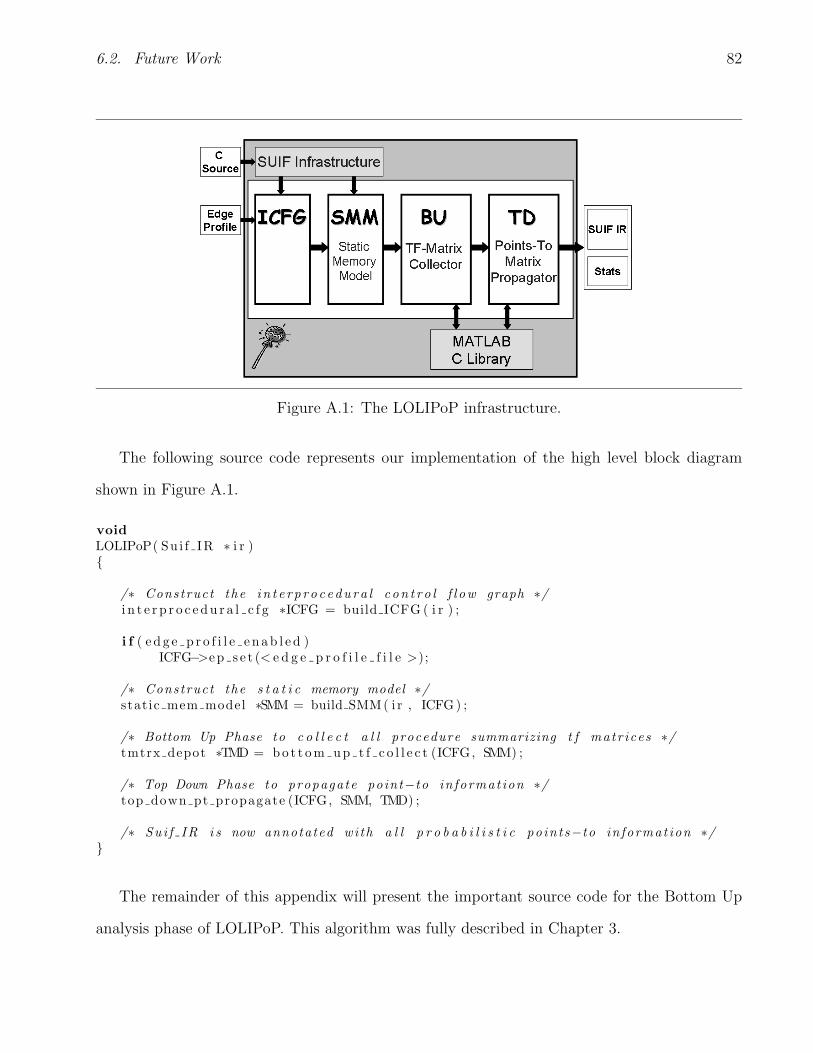
6.2. Future Work 82
Figure A.1: The LOLIPoP infrastructure.
The following source code represents our implementation of the high level block diagram
shown in Figure A.1.
void
LOLIPoP( Su i f IR ∗ i r ){
/∗ Construct the i n t e r p r o c edu ra l c on t r o l f l ow graph ∗/i n t e r p r o c e du r a l c f g ∗ICFG = build ICFG ( i r ) ;
i f ( e d g e p r o f i l e e n ab l e d )ICFG−>ep s e t (< e d g e p r o f i l e f i l e >);
/∗ Construct the s t a t i c memory model ∗/static mem model ∗SMM = build SMM( i r , ICFG) ;
/∗ Bottom Up Phase to c o l l e c t a l l procedure summarizing t f matr ices ∗/tmtrx depot ∗TMD = bo t t om up t f c o l l e c t (ICFG, SMM) ;
/∗ Top Down Phase to propagate point−to in format ion ∗/top down pt propagate (ICFG, SMM, TMD) ;
/∗ Sui f IR i s now annotated wi th a l l p r o b a b i l i s t i c po ints−to in format ion ∗/}
The remainder of this appendix will present the important source code for the Bottom Up
analysis phase of LOLIPoP. This algorithm was fully described in Chapter 3.

A.1. Suif Instruction to Transformation Matrix 83
A.1 Suif Instruction to Transformation Matrix
The following method summarizes a single SUIF instruction into a transformation matrix. Only
the unsafe version of this method is presented here.
t r an s f e r f n mt r x ∗g e t t f mt rx ( S u i f i n s t r u c t i o n ∗ s i ){
i f ( ! ICFG−>h a s p o i n t s t o g r a p h s i d e e f f e c t s ( s i ) )return Ident i ty Mtrx ;
t r an s f e r f n mt r x ∗ tfm = Spar se Ident i ty Mtrx ;
/∗ Get matrix row−i d f o r the l o c a t i o n s e t on the l e f t s i d e o f the asgn . ∗/int l s l o c i d = StaticMemoryModel−>g e t l s l o c i d ( s i ) ;
/∗ Get matrix row−i d f o r the l o c a t i o n s e t on the r i g h t s i d e o f the asgn . ∗/int r s l o c i d = StaticMemoryModel−>g e t r s l o c i d ( s i ) ;
/∗ Construct the matrix ∗/
double p = 1 / StaticMemoryModel−>number o f ptrs ( l s l o c i d ) ;
i f ( l s l o c i d != r s l o c i d ){
tfm−>s e t ( l s l o c i d , l s l o c i d ) = 1 − p ;tfm−>s e t ( l s l o c i d , r s l o c i d ) = p ;
}
/∗ Handle func t i on c a l l i n s t r u c t i o n s ∗/i f ( s i−> i s f u n c t i o n c a l l ){
S u i f f u n c t i o n c a l l ∗ f c = s i−>g e t f u n c t i o n c a l l ( )tfm = tfm ∗ g e t t f mt rx ( f c ) ;
}
return tfm ;}
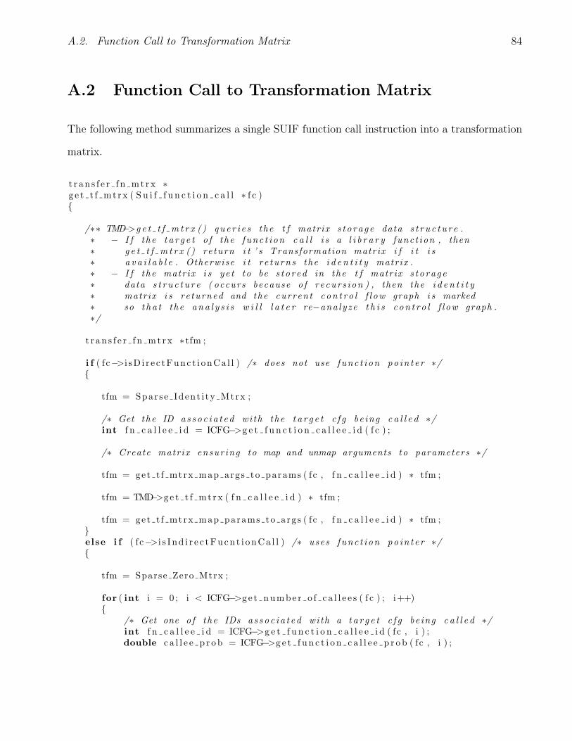
A.2. Function Call to Transformation Matrix 84
A.2 Function Call to Transformation Matrix
The following method summarizes a single SUIF function call instruction into a transformation
matrix.
t r an s f e r f n mt r x ∗g e t t f mt rx ( S u i f f u n c t i o n c a l l ∗ f c ){
/∗∗ TMD−>g e t t f m t r x ( ) qu e r i e s the t f matrix s t o rage data s t r u c t u r e .∗ − I f the t a r g e t o f the func t i on c a l l i s a l i b r a r y funct ion , then∗ g e t t f m t r x ( ) re turn i t ’ s Transformation matrix i f i t i s∗ a v a i l a b l e . Otherwise i t r e turns the i d e n t i t y matrix .∗ − I f the matrix i s ye t to be s t o r ed in the t f matrix s t o rage∗ data s t r u c t u r e ( occurs because o f r ecur s ion ) , then the i d e n t i t y∗ matrix i s re turned and the current c on t r o l f l ow graph i s marked∗ so t ha t the ana l y s i s w i l l l a t e r re−ana lyze t h i s c on t r o l f l ow graph .∗/
t r an s f e r f n mt r x ∗ tfm ;
i f ( fc−>i sD i r e c tFunc t i onCa l l ) /∗ does not use func t i on po in t e r ∗/{
tfm = Spar se Ident i ty Mtrx ;
/∗ Get the ID as s o c i a t e d wi th the t a r g e t c f g be ing c a l l e d ∗/int f n c a l l e e i d = ICFG−>g e t f u n c t i o n c a l l e e i d ( f c ) ;
/∗ Create matrix ensur ing to map and unmap arguments to parameters ∗/
tfm = get t f mtrx map args to params ( fc , f n c a l l e e i d ) ∗ tfm ;
tfm = TMD−>g e t t f mt rx ( f n c a l l e e i d ) ∗ tfm ;
tfm = get t f mtrx map params to args ( fc , f n c a l l e e i d ) ∗ tfm ;}else i f ( fc−>i s I nd i r e c tFucn t i onCa l l ) /∗ uses func t i on po in t e r ∗/{
tfm = Sparse Zero Mtrx ;
for ( int i = 0 ; i < ICFG−>g e t numbe r o f c a l l e e s ( f c ) ; i++){
/∗ Get one o f the IDs a s s o c i a t e d wi th a t a r g e t c f g be ing c a l l e d ∗/int f n c a l l e e i d = ICFG−>g e t f u n c t i o n c a l l e e i d ( fc , i ) ;double c a l l e e p r o b = ICFG−>g e t f u n c t i o n c a l l e e p r o b ( fc , i ) ;
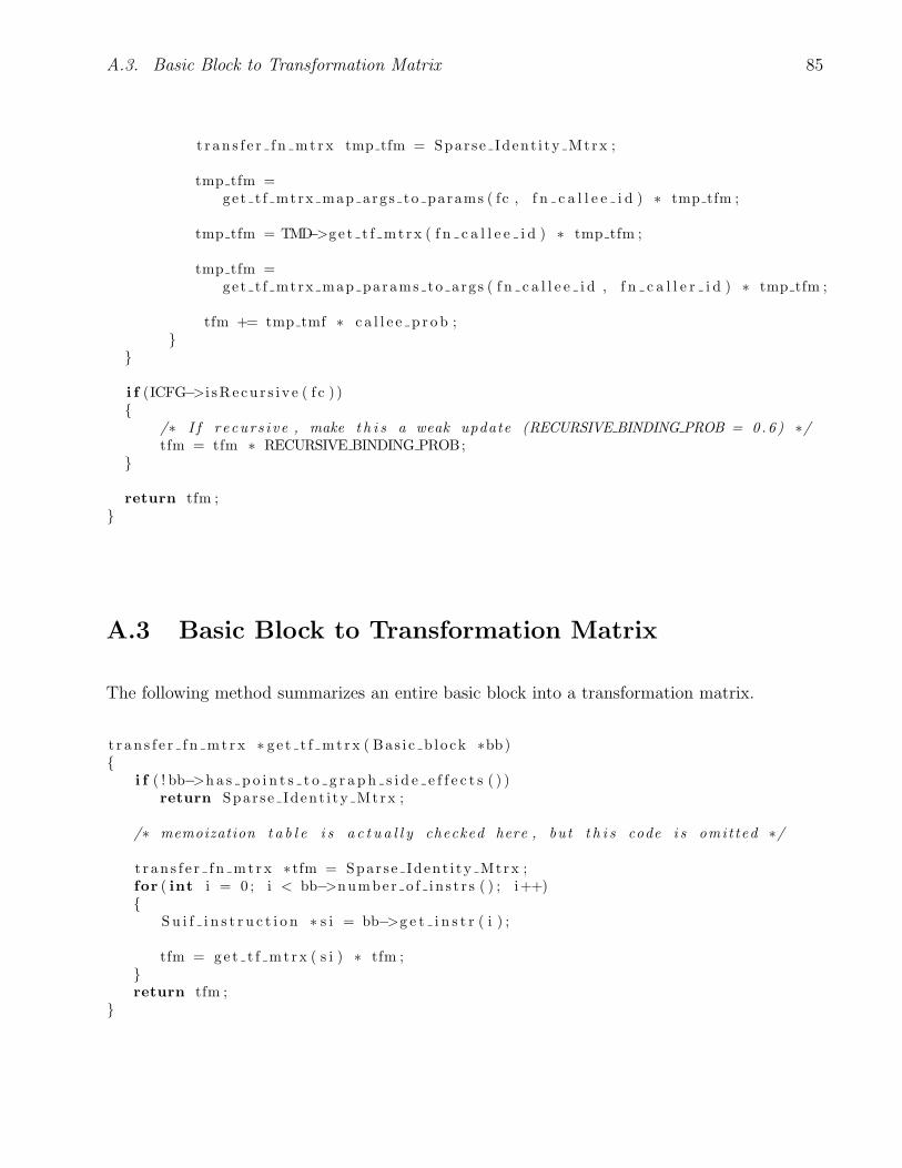
A.3. Basic Block to Transformation Matrix 85
t r an s f e r f n mt r x tmp tfm = Spar se Ident i ty Mtrx ;
tmp tfm =get t f mtrx map args to params ( fc , f n c a l l e e i d ) ∗ tmp tfm ;
tmp tfm = TMD−>g e t t f mt rx ( f n c a l l e e i d ) ∗ tmp tfm ;
tmp tfm =get t f mtrx map params to args ( f n c a l l e e i d , f n c a l l e r i d ) ∗ tmp tfm ;
tfm += tmp tmf ∗ c a l l e e p r o b ;}
}
i f (ICFG−>i sRe cu r s i v e ( f c ) ){
/∗ I f r e cur s i v e , make t h i s a weak update (RECURSIVE BINDING PROB = 0.6) ∗/tfm = tfm ∗ RECURSIVE BINDING PROB;
}
return tfm ;}
A.3 Basic Block to Transformation Matrix
The following method summarizes an entire basic block into a transformation matrix.
t r an s f e r f n mt r x ∗ g e t t f mt rx ( Bas i c b l o ck ∗bb){
i f ( ! bb−>h a s p o i n t s t o g r a p h s i d e e f f e c t s ( ) )return Spar se Ident i ty Mtrx ;
/∗ memoization t a b l e i s a c t u a l l y checked here , but t h i s code i s omit ted ∗/
t r an s f e r f n mt r x ∗ tfm = Spar se Ident i ty Mtrx ;for ( int i = 0 ; i < bb−>number o f i n s t r s ( ) ; i++){
Su i f i n s t r u c t i o n ∗ s i = bb−>g e t i n s t r ( i ) ;
tfm = ge t t f mt rx ( s i ) ∗ tfm ;}return tfm ;
}
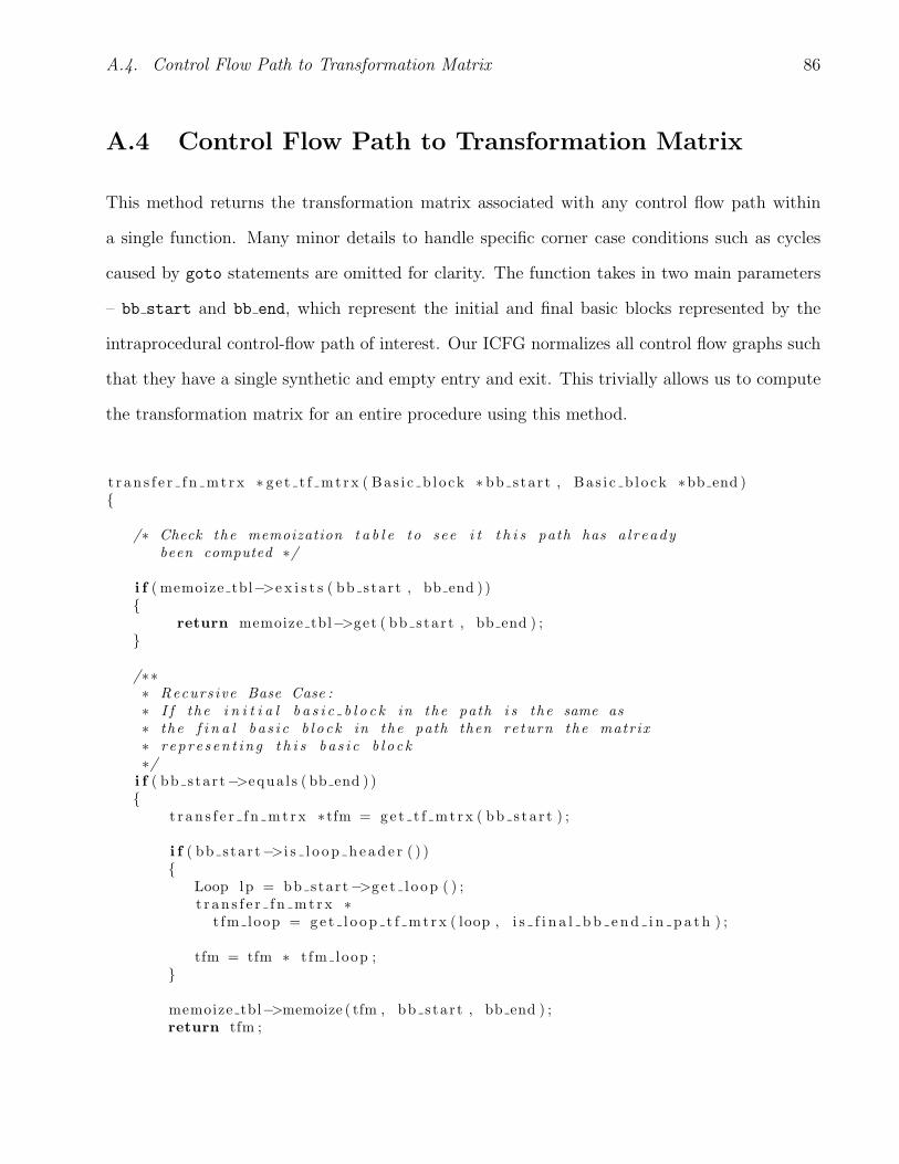
A.4. Control Flow Path to Transformation Matrix 86
A.4 Control Flow Path to Transformation Matrix
This method returns the transformation matrix associated with any control flow path within
a single function. Many minor details to handle specific corner case conditions such as cycles
caused by goto statements are omitted for clarity. The function takes in two main parameters
– bb start and bb end, which represent the initial and final basic blocks represented by the
intraprocedural control-flow path of interest. Our ICFG normalizes all control flow graphs such
that they have a single synthetic and empty entry and exit. This trivially allows us to compute
the transformation matrix for an entire procedure using this method.
t r an s f e r f n mt r x ∗ g e t t f mt rx ( Bas i c b l o ck ∗ bb star t , Bas i c b l o ck ∗bb end ){
/∗ Check the memoization t a b l e to see i t t h i s path has a l r eadybeen computed ∗/
i f ( memoize tbl−>e x i s t s ( bb s tar t , bb end ) ){
return memoize tbl−>get ( bb star t , bb end ) ;}
/∗∗∗ Recurs ive Base Case :∗ I f the i n i t i a l b a s i c b l o c k in the path i s the same as∗ the f i n a l b a s i c b l o c k in the path then re turn the matrix∗ r ep r e s en t i n g t h i s b a s i c b l o c k∗/
i f ( bb s tar t−>equa l s ( bb end ) ){
t r an s f e r f n mt r x ∗ tfm = ge t t f mt rx ( bb s t a r t ) ;
i f ( bb s tar t−>i s l o o p h e ad e r ( ) ){
Loop lp = bb star t−>ge t l o op ( ) ;t r an s f e r f n mt r x ∗
t fm loop = ge t l o op t f mt r x ( loop , i s f i n a l b b e n d i n p a t h ) ;
tfm = tfm ∗ t fm loop ;}
memoize tbl−>memoize ( tfm , bb star t , bb end ) ;return tfm ;

A.4. Control Flow Path to Transformation Matrix 87
}
/∗ Get the d i r e c t dominator o f bb end ∗/Bas i c b l o ck bb end dd = ICFG−>ge t d i r e c t domina to r ( bb end ) ;
/∗∗∗ Recurs ive c a l l to g e t the t f matrix r epre sen t ed by the path∗ from b b s t a r t to bb end ’ s d i r e c t dominator (=> t fm s t a r t t o e n d d d )∗/
t r an s f e r f n mt r x ∗ t fm s ta r t t o end dd = ge t t f mt rx ( bb star t , bb end dd ) ;
/∗∗∗ We now must compute the t f matrix r epre sen t ed by the path∗ from bb end ’ s d i r e c t dominator to bb end (=> t fm end dd to end )∗/
t r an s f e r f n mt r x ∗ t fm end dd to end = Sparse Zero Mtrx ;
for ( int i = 0 ; i < bb end−>num or predeces sor s ; i++){
t r an s f e r f n mt r x ∗tfm tmp = ge t t f mt rx ( bb end dd , bb end−>g e t p r ed e c e s s o r ( i ) ) ;
/∗ s c a l e the matrix based on the fan−in edge p r o b a b i l i t y ∗/tfm tmp ∗=
ICFG−>g e t f a n i n e d g e p r o b ab i l i t y ( bb end−>g e t p r ed e c e s s o r ( i ) , bb end ) ;
t fm end dd to end += tfm tmp ;}
t r an s f e r f n mt r x ∗ tfm end = ge t t f mt rx ( bb end ) ;
i f ( bb end−>i s l o o p h e ad e r ( ) ){
Loop lp = bb end−>ge t l o op ( ) ;t r an s f e r f n mt r x ∗
t fm loop = ge t l o op t f mt r x ( loop , i s f i n a l b b e n d i n p a t h ) ;
tfm end = tfm end ∗ t fm loop ;}
tm end dd to end = tfm end ∗ tm end dd to end ;
/∗ Compute the f i n a l t rans format ion matrix ∗/t r an s f e r f n mt r x ∗ tfm = tm end dd to end ∗ tm sta r t to end dd

A.4. Control Flow Path to Transformation Matrix 88
/∗ Memoize t h i s r e s u l t ∗/memoize tbl−>memoize ( tfm , bb star t , bb end ) ;
return tfm ;}

Appendix B
LOLIPoP from the Command Line
LOLIPoP is a command line utility invoked with the command ppa. The ppa utility takes in
a suif-linked SUIF-IR formatted file (*.spl) as an input and generates an annotated SUIF-IR
file (*.spx). In this appendix we list the various runtime options available to the user. Here we
show what prints out when a user invokes the ppa --help command.
Usage: ppa -.{OUTPUT_SUFFIX} [OPTIONS] [FILES]
For every pointer dereference, this analysis probabilistically identifies
which static location sets are being referenced.
Example:
scc -.spd file1.c file2.c file3.c
linksuif file1.spd file1.spl file2.spd file2.spl file3.spd file3.spl
ppa -.spx file1.spl file2.spl file3.spl
OPTIONS:
[--help], defines the various feature enabling flags
provided by this application
[-ppa_debug], outputs debugging & warning information
[-output_file <string>], specify PPA pointer dereference results
89
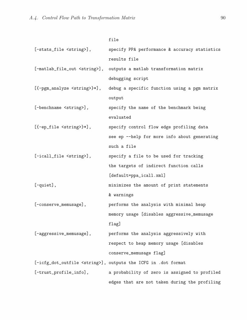
A.4. Control Flow Path to Transformation Matrix 90
file
[-stats_file <string>], specify PPA performance & accuracy statistics
results file
[-matlab_file_out <string>], outputs a matlab transformation matrix
debugging script
[{-pgm_analyze <string>}*], debug a specific function using a pgm matrix
output
[-benchname <string>], specify the name of the benchmark being
evaluated
[{-ep_file <string>}*], specify control flow edge profiling data
see ep --help for more info about generating
such a file
[-icall_file <string>], specify a file to be used for tracking
the targets of indirect function calls
[default=ppa_icall.xml]
[-quiet], minimizes the amount of print statements
& warnings
[-conserve_memusage], performs the analysis with minimal heap
memory usage [disables aggressive_memusage
flag]
[-aggressive_memusage], performs the analysis aggressively with
respect to heap memory usage [disables
conserve_memusage flag]
[-icfg_dot_outfile <string>], outputs the ICFG in .dot format
[-trust_profile_info], a probability of zero is assigned to profiled
edges that are not taken during the profiling

A.4. Control Flow Path to Transformation Matrix 91
phase
[-merge_heap_callsites], merges all heap callsites into one location
set
[-merge_temp_strings], merges all temp string variables into one
location set
[-field_sensitive], enables field sensitivity for C structs
[-pt_contexts <int>], specify the number of points-To contexts
per function to be stored [default=1]
[-use_inaccurate_gstf], enables a faster (unsound) geometric series
transform
[-phase_execute <int>], indicates upto which phase the analysis
should execute: 1 - build ICFG; 2 - build
Static Memory Model; 3 - Bottom Up Analysis;
4 - Top Down Analysis; [default=4; executes
all 4 phases]
[-evaluate_unreachable], forces the analysis of functions that are
statically deemed unreachable
[-safe_sva], perform shadow variable alias (sva) analysis
(makes the analysis multi-level safe)
[-blobs_supported <int>], when performing sva, specify the maximum
number of blobs that can be used [default=5]
[-blob_size_threshold <int>], when performing sva, specify the minimum
blob size [default=15]
[{-custom_alloc <string>}*] specify custom allocator functions that
return unique heap memory

Appendix C
Matrix Exponentiation and Geometric
Series Transformations
This appendix explains how the matrix geometric series operation can be directly mapped to
solving the exponentiation operation. A given loop has a transformation matrix equal to An,
where A is the transformation represented by the body of the loop and n is the number of
iterations. For example, consider the transformations that are applied to a simple for loop:
for ( i = 0 ; i < k ; i++){
. . .}
CASE 1 Assuming the loop has an inner transformation matrix defined by the square n × n
matrix A and the loop iterates a constant k times. Therefore the overall transformation matrix
defined by this for loop is equal to Ak. Ak can be efficiently computed using diagonalization or
eigenvalue decomposition.
Definition A square matrix A is diagonizable if there is an invertible matrix P such that
P−1AP is a diagonal matrix; the matrix P is said to diagonalize A.
92

A.4. Control Flow Path to Transformation Matrix 93
D = P−1AP
A = PDP−1
This can be used in computing powers of a matrix:
A2 = PDP−1PDP−1
A2 = PDIDP−1
A2 = PD2P−1
In General, for any positive integer k:
Ak = PDkP−1
Using this property, taking a power of a diagonal matrix is trivial.
Dk =
dk1 0 . . . 0
0 dk2 . . . 0
......
. . ....
0 0 . . . dkn
CASE 2 Assuming the loop has an inner transformation matrix defined by the square n × n
matrix A and the loop iterates a variable amount of times ranging from 0 to k. Therefore
the overall transformation matrix defined the by this for loop is equal to 1k+1
∑ki=0 Ai. This
geometric series expression can also be efficiently computed using diagonalization.
1k+1
∑ki=0 Ai = 1
k+1[A0 + A1 + A2 + ... + Ak]
1k+1
∑ki=0 Ai = 1
k+1[PD0P−1 + PD1P−1 + PD2P−1 + ... + PDkP−1]
1k+1
∑ki=0 Ai = 1
k+1P [D0 + D1 + D2 + ... + Dk]P−1
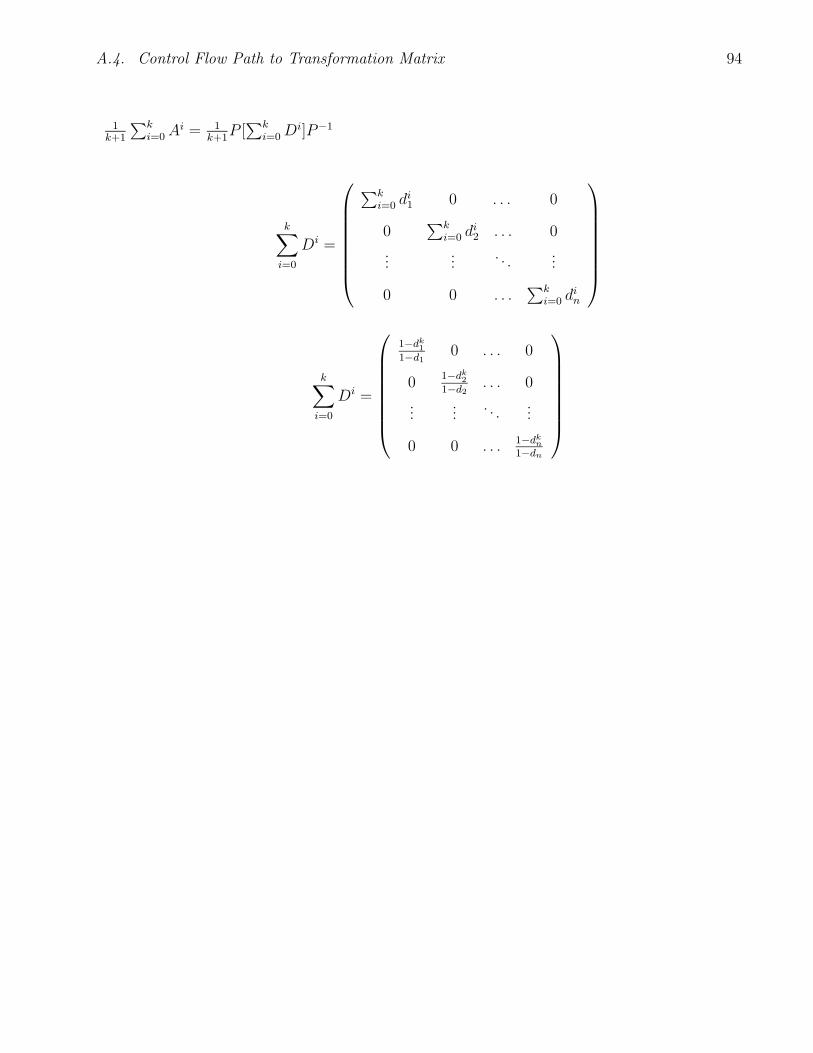
A.4. Control Flow Path to Transformation Matrix 94
1k+1
∑ki=0 Ai = 1
k+1P [
∑ki=0 Di]P−1
k∑
i=0
Di =
∑ki=0 di
1 0 . . . 0
0∑k
i=0 di2 . . . 0
......
. . ....
0 0 . . .∑k
i=0 din
k∑
i=0
Di =
1−dk
1
1−d1
0 . . . 0
01−dk
2
1−d2
. . . 0
......
. . ....
0 0 . . .1−dk
n
1−dn

Bibliography
[1] Alfred V. Aho, Ravi Sethi, and Jeffrey D. Ullman. Compilers: Princiles, Techniques, and
Tools. Addison-Wesley, 1986.
[2] L. Andersen. Program Analysis and Specialization for the C Programming Language. PhD
thesis, University of Copenhagen, May 1994. DIKU report 94/19.
[3] J. Gregory Steffan Antonia Zhai, Christopher B. Colohan and Todd C. Mowry. Compiler
optimization of scalar value communication between speculative threads. In Proccedings of
the Tenth International Conference on Architectural Support for Programming Languages
and Operating Systems, October 2002.
[4] J. Gregory Steffan Antonia Zhai, Christopher B. Colohan and Todd C. Mowry. Compiler
optimization of memory-resident value communication between speculative threads. In
Proceedings of the 2004 International Symposium on Code Generation and Optimization,
March 2004.
[5] Emery D. Berger, Benjamin G. Zorn, and Kathryn S. McKinley. Reconsidering custom
memory allocation. In OOPSLA ’02: Proceedings of the 17th ACM SIGPLAN conference
on Object-oriented programming, systems, languages, and applications, pages 1–12, New
York, NY, USA, 2002. ACM Press.
95

Bibliography 96
[6] Marc Berndl, Ondrej Lhotak, Feng Qian, Laurie Hendren, and Navindra Umanee. Points-to
analysis using bdds. In PLDI ’03: Proceedings of the ACM SIGPLAN 2003 conference on
Programming language design and implementation, pages 103–114, New York, NY, USA,
2003. ACM Press.
[7] Anasua Bhowmik and Manoj Franklin. A fast approximate interprocedural analysis for
speculative multithreading compilers. In ICS ’03: Proceedings of the 17th annual inter-
national conference on Supercomputing, pages 32–41, New York, NY, USA, 2003. ACM
Press.
[8] Johann Blieberger, Bernd Burgstaller, and Bernhard Scholz. Interprocedural symbolic
evaluation of ada programs with aliases. In Ada-Europe ’99: Proceedings of the 1999 Ada-
Europe International Conference on Reliable Software Technologies, pages 136–145, London,
UK, 1999. Springer-Verlag.
[9] Gunilla Borgefors, Giuliana Ramella, and Gabriella Sanniti di Baja. Using top-down and
bottom-up analysis for a multiscale skeleton hierarchy. In ICIAP ’97: Proceedings of the
9th International Conference on Image Analysis and Processing-Volume I, pages 369–376,
London, UK, 1997. Springer-Verlag.
[10] Randal E. Bryant. Graph-based algorithms for boolean function manipulation. IEEE
Transactions on Computers, 35(8):677–691, 1986.
[11] Dov Bulka and David Mayhew. Efficient C++ : Performance Programming Techniques.
Addison Wesley, November 1999.
[12] Ramkrishna Chatterjee, Barbara G. Ryder, and William A. Landi. Relevant context in-
ference. In POPL ’99: Proceedings of the 26th ACM SIGPLAN-SIGACT symposium on
Principles of programming languages, pages 133–146, New York, NY, USA, 1999. ACM
Press.

Bibliography 97
[13] Peng-Sheng Chen, Ming-Yu Hung, Yuan-Shin Hwang, Roy Dz-Ching Ju, and Jenq Kuen
Lee. Compiler support for speculative multithreading architecture with probabilistic points-
to analysis. SIGPLAN Not., 38(10):25–36, 2003.
[14] Peng-Sheng Chen, Yuan-Shin Hwang, Roy Dz-Ching Ju, and Jenq Kuen Lee. Interproce-
dural probabilistic pointer analysis. IEEE Trans. Parallel Distrib. Syst., 15(10):893–907,
2004.
[15] Ben-Chung Cheng and Wen-Mei W. Hwu. Modular interprocedural pointer analysis using
access paths: design, implementation, and evaluation. In PLDI ’00: Proceedings of the
ACM SIGPLAN 2000 conference on Programming language design and implementation,
pages 57–69, New York, NY, USA, 2000. ACM Press.
[16] Chakra Chennubhotla and Allan Jepson. Hierarchical eigensolver for transition matrices in
spectral methods. In Lawrence K. Saul, Yair Weiss, and Leon Bottou, editors, Advances
in Neural Information Processing Systems 17, pages 273–280. MIT Press, Cambridge, MA,
2005.
[17] Roy Dz ching Ju, Jean-Francois Collard, and Karim Oukbir. Probabilistic memory dis-
ambiguation and its application to data speculation. SIGARCH Comput. Archit. News,
27(1):27–30, 1999.
[18] Roy Dz ching Ju, Kevin Nomura, Uma Mahadevan, and Le-Chun Wu. A unified com-
piler framework for control and data speculation. In PACT ’00: Proceedings of the 2000
International Conference on Parallel Architectures and Compilation Techniques, page 157,
Washington, DC, USA, 2000. IEEE Computer Society.
[19] Standard Performance Evaluation Corporation. The spec benchmark suite. Technical
report, Standard Performance Evaluation Corporation. http://www.spechbench.org.

Bibliography 98
[20] Xiaoru Dai, Antonia Zhai, Wei-Chung Hsu, and Pen-Chung Yew. A general compiler
framework for speculative optimizations using data speculative code motion. In CGO,
pages 280–290, 2005.
[21] Manuvir Das. Unification-based pointer analysis with directional assignments. In PLDI
’00: Proceedings of the ACM SIGPLAN 2000 conference on Programming language design
and implementation, pages 35–46, New York, NY, USA, 2000. ACM Press.
[22] Manuvir Das, Ben Liblit, Manuel Fahndrich, and Jakob Rehof. Estimating the impact of
scalable pointer analysis on optimization. In SAS ’01: Proceedings of the 8th International
Symposium on Static Analysis, pages 260–278, London, UK, 2001. Springer-Verlag.
[23] Amer Diwan, Kathryn S. McKinley, and J. Eliot B. Moss. Type-based alias analysis. In
PLDI ’98: Proceedings of the ACM SIGPLAN 1998 conference on Programming language
design and implementation, pages 106–117, New York, NY, USA, 1998. ACM Press.
[24] Carole Dulong. The ia-64 architecture at work. Computer, 31(7):24–32, 1998.
[25] Stanley C. Eisenstat and Andrew H. Sherman. Efficient implementation of sparse nonsym-
metric gaussian elimination without pivoting. In Proceedings of the SIGNUM meeting on
Software for partial differential equations, pages 26–29, New York, NY, USA, 1975. ACM
Press.
[26] Maryam Emami, Rakesh Ghiya, and Laurie J. Hendren. Context-sensitive interprocedural
points-to analysis in the presence of function pointers. In PLDI ’94: Proceedings of the
ACM SIGPLAN 1994 conference on Programming language design and implementation,
pages 242–256, New York, NY, USA, 1994. ACM Press.
[27] Manuel Fahndrich, Jeffrey S. Foster, Zhendong Su, and Alexander Aiken. Partial online
cycle elimination in inclusion constraint graphs. In PLDI ’98: Proceedings of the ACM
Bibliography 99
SIGPLAN 1998 conference on Programming language design and implementation, pages
85–96, New York, NY, USA, 1998. ACM Press.
[28] Manuel Fahndrich, Jakob Rehof, and Manuvir Das. Scalable context-sensitive flow analysis
using instantiation constraints. In PLDI ’00: Proceedings of the ACM SIGPLAN 2000
conference on Programming language design and implementation, pages 253–263, New York,
NY, USA, 2000. ACM Press.
[29] Manel Fernandez and Roger Espasa. Speculative alias analysis for executable code. In
PACT ’02: Proceedings of the 2002 International Conference on Parallel Architectures and
Compilation Techniques, pages 222–231, Washington, DC, USA, 2002. IEEE Computer
Society.
[30] M. Franklin and G. S. Sohi. Arb: A hardware mechanism for dynamic reordering of memory
references. IEEE Transactions on Computers, May 1996.
[31] Manoj Franklin. The Multiscalar Architecture. PhD thesis, Department of Computer Sci-
ences, University of Wisconsin-Madison, December 1993.
[32] S. Breach G. S. Sohi and T. N. Vijaykumar. Multiscalar processors. In Proceedings of the
22th International Symposium on Computer Architecture, June 1995.
[33] Rakesh Ghiya and Laurie J. Hendren. Is it a tree, a dag, or a cyclic graph? a shape analysis
for heap-directed pointers in c. In POPL ’96: Proceedings of the 23rd ACM SIGPLAN-
SIGACT symposium on Principles of programming languages, pages 1–15, New York, NY,
USA, 1996. ACM Press.
[34] Abhijit Ghosh, Joachim Kunkel, and Stan Liao. Hardware synthesis from c/c++. In DATE
’99: Proceedings of the conference on Design, automation and test in Europe, page 82, New
York, NY, USA, 1999. ACM Press.

Bibliography 100
[35] John R. Gilbert, Cleve Moler, and Robert Schreiber. Sparse matrices in MATLAB: Design
and implementation. SIAM Journal on Matrix Analysis and Applications, 13(1):333–356,
1992.
[36] Sridhar Gopal, T.N. Vijaykumar, J. E. Smith, and G. S. Sohi. Speculative versioning cache.
In Proceedings of the Fourth International Symposium on High-Performance Computer Ar-
chitecture, February 1998.
[37] Lance Hammond, Brian D. Carlstrom, Vicky Wong, Mike Chen, Christos Kozyrakis, and
Kunle Olukotun. Transactional coherence and consistency: Simplifying parallel hardware
and software. Mico’s Top Picks, IEEE Micro, 24(6), nov/dec 2004.
[38] Lance Hammond, Brian D. Carlstrom, Vicky Wong, Ben Hertzberg, Mike Chen, Christos
Kozyrakis, and Kunle Olukotun. Programming with transactional coherence and consis-
tency (tcc). In Proceedings of the 11th International Conference on Architectural Support
for Programming Languages and Operating Systems, pages 1–13. ACM Press, Oct 2004.
[39] Lance Hammond, Ben Hubbert, Michael Siu, Manohar Prabhu, Mike Chen, and Kunle
Olukotun. The stanford hydra cmp. In IEEE MICRO Magazine, March 2000.
[40] Lance Hammond, Mark Willey, and Kunle Olukotun. Data speculation support for a chip
multiprocessor. In Proceedings of the Eighth ACM Conference on Architectural Support for
Programming Languages and Operating Systems, October 1998.
[41] Desmond J. Higham and Nicholas J. Higham. MATLAB Guide. Society for Industrial and
Applied Mathematics, Philadelphia, PA, USA, 2000.
[42] Michael Hind. Pointer analysis: haven’t we solved this problem yet? In PASTE ’01: Pro-
ceedings of the 2001 ACM SIGPLAN-SIGSOFT workshop on Program analysis for software
tools and engineering, pages 54–61, New York, NY, USA, 2001. ACM Press.
Bibliography 101
[43] Michael Hind, Michael Burke, Paul Carini, and Jong-Deok Choi. Interprocedural pointer
alias analysis. ACM Trans. Program. Lang. Syst., 21(4):848–894, 1999.
[44] Michael Hind and Anthony Pioli. Which pointer analysis should i use? In ISSTA ’00:
Proceedings of the 2000 ACM SIGSOFT international symposium on Software testing and
analysis, pages 113–123, New York, NY, USA, 2000. ACM Press.
[45] Intel Corporation. IA-64 Application Developer’s Architecture Guide. May 1999.
[46] N. P. Jouppi and D. W. Wall. Available instruction-level parallelism for superscalar and
superpipelined machines. In ASPLOS-III: Proceedings of the third international conference
on Architectural support for programming languages and operating systems, pages 272–282,
New York, NY, USA, 1989. ACM Press.
[47] Venkata Krishnan and Josep Torrellas. A chip multiprocessor architecture with specu-
lative multithreading. IEEE Transactions on Computers, Special Issue on Multithreaded
Architecture, September 1999.
[48] William Landi and Barbara G. Ryder. Pointer-induced aliasing: a problem taxonomy. In
POPL ’91: Proceedings of the 18th ACM SIGPLAN-SIGACT symposium on Principles of
programming languages, pages 93–103, New York, NY, USA, 1991. ACM Press.
[49] William Landi and Barbara G. Ryder. A safe approximate algorithm for interprocedural
pointer aliasing. In Proceedings of the Conference on Programming Language Design and
Implementation (PLDI), volume 27, pages 235–248, New York, NY, 1992. ACM Press.
[50] Chris Lattner and Vikram Adve. Automatic pool allocation: improving performance by
controlling data structure layout in the heap. SIGPLAN Not., 40(6):129–142, 2005.
[51] Jin Lin, Tong Chen, Wei-Chung Hsu, and Pen-Chung Yew. Speculative register promotion
using advanced load address table (alat). In CGO ’03: Proceedings of the international

Bibliography 102
symposium on Code generation and optimization, pages 125–134, Washington, DC, USA,
2003. IEEE Computer Society.
[52] Jin Lin, Tong Chen, Wei-Chung Hsu, Pen-Chung Yew, Roy Dz-Ching Ju, Tin-Fook Ngai,
and Sun Chan. A compiler framework for speculative analysis and optimizations. In PLDI
’03: Proceedings of the ACM SIGPLAN 2003 conference on Programming language design
and implementation, pages 289–299, New York, NY, USA, 2003. ACM Press.
[53] The MathWorks, Inc. MATLAB C Math Library Reference, version 2 edition, January
1999.
[54] Markus Mock, Manuvir Das, Craig Chambers, and Susan J. Eggers. Dynamic points-to sets:
a comparison with static analyses and potential applications in program understanding and
optimization. In PASTE ’01: Proceedings of the 2001 ACM SIGPLAN-SIGSOFT workshop
on Program analysis for software tools and engineering, pages 66–72, New York, NY, USA,
2001. ACM Press.
[55] Markus Mock, Ricardo Villamarin, and Jose Baiocchi. An empirical study of data specu-
lation use on the intel itanium 2 processor. In INTERACT ’05: Ninth Annual Workshop
on Interaction between Compilers and Computer Architectures, pages 22–33, 2005.
[56] Steven S. Muchnick. Advanced Compiler Design and Implementation. Morgan Kaufmann,
1997.
[57] Erik M. Nystrom, Hong-Seok Kim, and Wen mei W. Hwu. Importance of heap specialization
in pointer analysis. In PASTE ’04: Proceedings of the ACM-SIGPLAN-SIGSOFT workshop
on Program analysis for software tools and engineering, pages 43–48, New York, NY, USA,
2004. ACM Press.
Bibliography 103
[58] G. Ramalingam. The undecidability of aliasing. ACM Trans. Program. Lang. Syst.,
16(5):1467–1471, 1994.
[59] G. Ramalingam. Data flow frequency analysis. In PLDI ’96: Proceedings of the ACM
SIGPLAN 1996 conference on Programming language design and implementation, pages
267–277, New York, NY, USA, 1996. ACM Press.
[60] Amir Roth and Gurindar S. Sohi. Speculative data-driven multithreading. In Proceedings
of the 7th International Symposium on High Performance Computer Architecture, January
2001.
[61] Atanas Rountev and Satish Chandra. Off-line variable substitution for scaling points-to
analysis. In PLDI ’00: Proceedings of the ACM SIGPLAN 2000 conference on Programming
language design and implementation, pages 47–56, New York, NY, USA, 2000. ACM Press.
[62] Radu Rugina and Martin Rinard. Pointer analysis for multithreaded programs. In PLDI
’99: Proceedings of the ACM SIGPLAN 1999 conference on Programming language design
and implementation, pages 77–90, New York, NY, USA, 1999. ACM Press.
[63] Karthikeyan Sankaralingam, Ramadass Nagarajan, Haiming Liu, Changkyu Kim, Jaehyuk
Huh, Nitya Ranganathan, Doug Burger, Stephen W. Keckler, Robert G. McDonald, and
Charles R. Moore. Trips: A polymorphous architecture for exploiting ilp, tlp, and dlp.
ACM Trans. Archit. Code Optim., 1(1):62–93, 2004.
[64] Luc Semeria and Giovanni De Micheli. Spc: synthesis of pointers in c: application of
pointer analysis to the behavioral synthesis from c. In ICCAD ’98: Proceedings of the 1998
IEEE/ACM international conference on Computer-aided design, pages 340–346, New York,
NY, USA, 1998. ACM Press.

Bibliography 104
[65] Bjarne Steensgaard. Points-to analysis in almost linear time. In POPL ’96: Proceedings
of the 23rd ACM SIGPLAN-SIGACT symposium on Principles of programming languages,
pages 32–41, New York, NY, USA, 1996. ACM Press.
[66] J. Gregory Steffan. Hardware Support for Thread-Level Speculation. PhD thesis, School of
Computer Science, Carnegie Mellon University, April 2003.
[67] J. Gregory Steffan, Christopher B. Antonia, Colohan Zhai, and Todd C. Mowry. A scalable
approach to thread-level speculation. In Proceedings of the 27th International Symposium
on Computer Architecture, June 2000.
[68] J. Gregory Steffan, Christopher B. Colohan, Antonia Zhai, and Todd C. Mowry. Improving
value communication for thread-level speculation. In Proceedings of the Eighth International
Symposium on High-Performance Computer Architecture, February 2002.
[69] J. Gregory Steffan, Christopher B. Colohan, Antonia Zhai, and Todd C. Mowry. The
stampede approach to thread-level speculation. ACM Transactions on Computer Systems,
23(3):253–300, August 2005.
[70] Philip A. Stocks, Barbara G. Ryder, William A. Landi, and Sean Zhang. Comparing flow
and context sensitivity on the modification-side-effects problem. In ISSTA ’98: Proceedings
of the 1998 ACM SIGSOFT international symposium on Software testing and analysis,
pages 21–31, New York, NY, USA, 1998. ACM Press.
[71] Steven Swanson, Ken Michelson, Andrew Schwerin, and Mark Oskin. Wavescalar. In
MICRO 36: Proceedings of the 36th annual IEEE/ACM International Symposium on Mi-
croarchitecture, page 291, Washington, DC, USA, 2003. IEEE Computer Society.
Bibliography 105
[72] Robert Tarjan. Testing flow graph reducibility. In STOC ’73: Proceedings of the fifth annual
ACM symposium on Theory of computing, pages 96–107, New York, NY, USA, 1973. ACM
Press.
[73] Robert Endre Tarjan. Efficiency of a good but not linear set union algorithm. J. ACM,
22(2):215–225, 1975.
[74] S. Tjiang, M. Wolf, M. Lam, K. Pieper, and J. Hennessy. Languages and Compilers for
Parallel Computing, pages 137–151. Springer-Verlag, Berlin, Germany, 1992.
[75] T. N. Vijaykumar. Compiling for the Multiscalar Architecture. PhD thesis, Department of
Computer Sciences, University of Wisconsin-Madison, January 1998.
[76] Kazutoshi Wakabayashi. C-based synthesis experiences with a behavior synthesizer, cyber.
In DATE ’99: Proceedings of the conference on Design, automation and test in Europe,
page 83, New York, NY, USA, 1999. ACM Press.
[77] John Whaley and Monica S. Lam. Cloning-based context-sensitive pointer alias analysis
using binary decision diagrams. In PLDI ’04: Proceedings of the ACM SIGPLAN 2004
conference on Programming language design and implementation, pages 131–144, New York,
NY, USA, 2004. ACM Press.
[78] Robert P. Wilson and Monica S. Lam. Efficient context-sensitive pointer analysis for c pro-
grams. In PLDI ’95: Proceedings of the ACM SIGPLAN 1995 conference on Programming
language design and implementation, pages 1–12, New York, NY, USA, 1995. ACM Press.
[79] Youfeng Wu and Yong fong Lee. Accurate invalidation profiling for effective data speculation
on epic processors. In ISCA 13th International Conference on Parallel and Distributed
Computing Systems, Las Vegas, Nevada, USA, August 2000.

Bibliography 106
[80] Jianwen Zhu and Silvian Calman. Symbolic pointer analysis revisited. In PLDI ’04: Pro-
ceedings of the ACM SIGPLAN 2004 conference on Programming language design and
implementation, pages 145–157, New York, NY, USA, 2004. ACM Press.