Climatic ChangeDOI 10.1007/s10584-010-0001-9

Probabilistic life cycle analysis model for evaluatingelectric power infrastructure risk mitigation investments

Royce A. Francis · Stefanie M. Falconi ·Roshanak Nateghi · Seth D. Guikema

Received: 9 March 2010 / Accepted: 8 November 2010© Springer Science+Business Media B.V. 2010

Abstract One effect of climate change may be increased hurricane frequency orintensity due to changes in atmospheric and geoclimatic factors. It has been hypoth-esized that wetland restoration and infrastructure hardening measures may improveinfrastructure resilience to increased hurricane frequency and intensity. This paperdescribes a parametric decision model used to assess the tradeoffs between wetlandrestoration and infrastructure hardening for electric power networks. We employa hybrid economic input–output life-cycle analysis (EIO-LCA) model to capture:construction costs and life-cycle emissions for transitioning from the current electricpower network configuration to a hardened network configuration; constructioncosts and life-cycle emissions associated with wetland restoration; and the intrinsicvalue of wetland restoration. Uncertainty is accounted for probabilistically through aMonte Carlo hurricane simulation model and parametric sensitivity analysis for thenumber of hurricanes expected to impact the project area during the project cycle

R. A. Francis (B)Department of Engineering Management and Systems Engineering, The George WashingtonUniversity, 1776 G St., NW #159, Washington, DC 20059, USAe-mail: seed@gwu.edu

S. M. Falconi · R. Nateghi · S. D. GuikemaDepartment of Geography and Environmental Engineering, Johns Hopkins University,313 Ames Hall, 3400 N. Charles St., Baltimore, MD 21218, USA

S. M. Falconie-mail: stefanie.falconi@jhu.edu

R. Nateghie-mail: rnategh1@jhu.edu

S. D. GuikemaDepartment of Civil Engineering, Johns Hopkins University,313 Ames Hall, 3400 N. Charles St., Baltimore, MD 21218, USAe-mail: sguikema@jhu.edu

Climatic Change

and the rate of wetland storm surge attenuation. Our analysis robustly indicates thatwetland restoration and undergrounding of electric power network infrastructure isnot preferred to the “do-nothing” option of keeping all power lines overhead withoutwetland protection. However, we suggest a few items for future investigation. Forexample, our results suggest that, for the small case study developed, synergisticbenefits of simultaneously hardening infrastructure and restoring wetlands may belimited, although research using a larger test bed while integrating additional costsmay find an enhanced value of wetland restoration for disaster loss mitigation.

1 Introduction

Recently, climate change has been associated with potential increases in hurricanefrequency or intensity (Emanuel 2005). Increases in population density in coastalareas have also been forecasted (Nicholls and Small 2002; Small and Nicholls 2003),thus increasing the urgency of mitigating potential adverse outcomes associated withhurricane events. These observations have led risk managers to consider the effectsof increased hurricane frequency and intensity on networks of lifeline infrastruc-ture that support our societies (U.S. Congress Office of Technology Assessment1990). Examples of lifeline infrastructure networks include electric power networks,drinking water and wastewater networks, transportation networks, and oil and gaspipeline networks. Hurricane Katrina has further focused attention in the USA onthe potential adverse impacts of increased hurricane frequency and intensity (Dayet al. 2007), and attendant risk mitigation decisions are currently being re-evaluated(Bigger et al. 2009; U.S. Army Corps of Engineers 2004). It has been hypothesizedthat coastal wetland restoration may be a cost-effective approach to mitigating theimpacts of future hurricanes (Wamsley et al. 2009, 2010).

The objective of the analysis presented in this paper is to demonstrate a method-ology for evaluating potential risk mitigation synergies between coastal wetlandrestoration and infrastructure protection, focusing on electric power network hard-ening. We evaluate the life cycle costs associated with electric power networkhardening and wetland restoration for a model city case study for three scenarios:undergrounding all electric power equipment; undergrounding only electric powerequipment in the commercial zone; and making no changes to the existing networkconfiguration. For each of these scenarios, we evaluate life cycle costs with andwithout wetlands, and including and not including indirect economic and environ-mental costs. Our results suggest that for our case study city, wetland restorationand infrastructure hardening are not the preferred options. This result has importantimplications for coastal adaption planning. Natural ecosystem restoration may bedifficult to justify as an approach for coastal adaptation without separately consider-ing the valuation of biodiversity, ecological services, and carbon sequestration. Whilethese issues pose difficult valuation problems, the more directly quantifiable benefitsof wetland restoration may not offset the significant cost of restoring or buildingwetlands in many locations.

2 EIO-LCA disaster mitigation framework

Risk mitigation decisions are currently evaluated using several tools, including butnot limited to: benefit–cost analysis (BCA) (Arrow et al. 1996), life-cycle cost

Climatic Change

analysis (LCA) (Chang and Shinozuka 1996), and probabilistic decision analysis(Keeney 1982). BCA involves maximizing the ratio of benefits expected from adecision to the expected costs incurred by taking a decision. The assumption is thatmaximizing this ratio maximizes public welfare. LCA extends BCA by accountingfor the costs incurred over the life cycle of a project undertaken as a result of aspecific decision. Probabilistic decision analysis involves parameterizing the decisionchoices and probability of potential adverse outcomes to be mitigated such thatthe uncertainty associated with the occurrence of an adverse event is quantitativelyevaluated in the decision framework and the decisions are based on maximizingexpected utility. Risk mitigation decisions can be evaluated using a combinationof each of these tools. One recent disaster risk mitigation methodology proposedcombining each of these tools is the extended life cycle cost analysis framework(ELCA) (Chang 2003).

ELCA extends traditional approaches to BCA by incorporating societal costsand benefits over a risk mitigation project’s planned life with the benefits and costsexpected to accrue to the relevant lifeline agency over a project’s planned life. Thecomputation of societal and lifeline agency costs and benefits is facilitated by atransparent framework accounting for four types of costs and benefits (Chang 2003):planned costs undertaken by the lifeline agency; costs imposed on society by thelifeline agency’s actions; expected unplanned costs undertaken by the lifeline agency;and, expected unplanned costs imposed on society through lifeline service disruptionand restoration.

In the present paper, we extend the ELCA by incorporating supply-chain envi-ronmental impacts and other societal impacts associated with disaster risk mitigationprojects. To incorporate these environmental and societal impacts, the economicinput–output life-cycle assessment (EIO-LCA) framework (Hendrickson et al. 2006)is employed. We describe this new framework below in the section titled “EIO-LCA Disaster Mitigation Framework”. We then apply the extended ELCA to ahypothetical case study with three decision scenarios evaluating wetland restorationand electric power network hardening to mitigate electric power infrastructure riskin the event of increased hurricane frequency and intensity.

2.1 Extended ELCA framework

Chang and Shinozuka (1996) and Chang (2003) have extended the practice ofproject life-cycle cost analysis to disaster loss estimation methodology. We adapt thisframework for our purposes and present the details of its characterization here. Asdescribed above, this framework consists of four parts:

C = C1 + C2 + C3 + C4 (1)

where: C1 = planned costs undertaken by the lifeline agency; C2 = costs imposed onsociety by the lifeline agency’s actions; C3 = expected unplanned costs undertaken bythe lifeline agency; and, C4 = expected unplanned costs imposed on society throughlifeline service disruption and restoration.

The planned costs undertaken by the lifeline agency, C1, are the sum of direct coststo the utility of performing routine maintenance on the infrastructure network andthe costs to the utility of performing mitigation investments (with their associatedmaintenance costs). The maintenance and mitigation investments required dependon the nature of the network and the anticipated natural disaster. More specifically,

Climatic Change

the maintenance costs, Cm, are calculated as the sum of the maintenance cost mfor system element i, multiplied by a discount factor for year t, z(t), for all systemelements over the planned project life.

Cm =∑

t

∑

i

mi (xi, t) · z (t) (2)

The mitigation investment costs, Cmit, are calculated as the sum of the mitigationinvestment cost e for system element i, multiplied by the discount factor for year t forall system elements over the planned project life.

Cmit =∑

t

∑

i

ei (xi, t) · z (t) (3)

Both of these costs depend on properties of the system elements including their age,materials, and tasks required.

The costs imposed on society as a result of the lifeline utility’s mitigation decisions,C2, are the sum of the benefits associated with disaster mitigation activities (e.g.,increased employment and improved operational efficiency) and the environmentalimpacts associated with the activities required by the mitigation decisions. Changand Shinozuka (1996) and Chang (2003) included only the economic portion of thesecosts and benefits. Here we extend this to incorporate the life-cycle environmentalcosts of agency decisions.

To compute costs and benefits, we employ the EIO-LCA approach. In short, EIO-LCA adapts the Leontief input–output economic model to estimate the environmen-tal emissions associated with a product or service over its lifetime (Hendrickson et al.2006). Because the overall economic activity associated with a product or service overits lifetime is more inclusive than the revenue associated with its purchase, we cantake advantage of this feature of the EIO-LCA model to compute the environmentalcosts and economic benefits attributable to the lifeline agency’s mitigation decisions.We propose that the benefits, beyond risk mitigation, of the lifeline agency’s decisionare the additional economic output associated with maintenance and mitigationactivities above the direct costs to the lifeline agency, EOm and EOmit, respectively.In the event that wetland restoration is chosen, additional economic benefits accruedue to the economic value of the ecosystem services of the restored wetland area,EVwet. The costs imposed on society include the environmental costs and servicedisruptions associated with the maintenance and mitigation investments. In thispaper, we ignore the costs of the service disruptions due to maintenance andmitigation investments, including only the environmental costs, Rm and Rmit, of themaintenance and mitigation investments, respectively.

C2 =∑

t

[(EOm + EOmit + EVwet) − (Rm + Rmit)

]t · z (t) (4)

For the mathematical details of the EIO-LCA model, the reader is referred toHendrickson et al. (2006).

The expected lifeline utility costs in the event of a natural disaster, C3, are thesum of the expected repair costs associated with system element failures caused bythe natural disaster, Cr, and the revenue loss attributable to the attendant servicedisruptions, Cv .

C3 = Cr + Cv (5)

Climatic Change

As with Cm and Ce, the repair costs of a system element failure depend on theelement properties, age of the system element, and tasks required to perform therepair. Chang (2003) characterizes the expected repair costs of system element iover the project life as the sum of the product of the expected failure probability inevent of a natural disaster, Fi, and its unit repair cost ri for each system element overthe life of the project. The expected failure probability due to natural disasters overthe planned life of the project is computed by integrating the product of the systemelement’s fragility curve, PF , and the hazard curve for natural disasters, p(h), overthe range of possible disaster intensities, h. The hazard curve gives the probabilityof a hazard of intensity h occurring, and the fragility curve gives the probability ofelement failure as a function of h, system element age, and system element type.

Cr =∑

t

∑

i

[Fi (xi, t) · ri] · z (t)

Fi (xi, t) =∫

h

PF (xi, t, h) · p (h) dh (6)

The revenue loss attributable to attendant service disruptions, Cv , is the sum of theproduct of the expected annual unmet demand, Vt, and unit price, p, of the serviceprovided over life of the project. The unmet demand is a function of the time toservice restoration, τ , the percent initial unmet demand, ω, the normal demandvolume, D, the hazard curve for natural disaster intensity, and decision-makingfactors related to system repairs, w.

Cv =∑

t

Vt · p · z (t)

Vt =∫

h

τ (w, h) · ω (h) · D · p (h) dh (7)

Finally, the expected costs imposed on society in the event of a natural disaster, C4,are the sum of the losses in economic activity that occur from utility outage andcascading business losses directly caused by utility outages. As with the costs imposedon society due to routine maintenance and initial mitigation investments, C4 may bedivided into the economic output and environmental costs. We include the economicoutput, EOr, caused by the repairs Cr, the economic output lost, EOl , due to directbusiness losses, CB, and the lost economic output, EOul , associated with decreasedutility revenues, Cv . We also account for the environmental costs associated withrepairs, Rr, and the reduction in environmental costs due to direct business losses,Rl , and service interruptions, Rul .

C4 =∑

t

[{EOr (Cr) − EOl (CB) − EOul (Cv)} − {Rr − Rl − Rul}]

t · z (t) (8)

While we have defined the repair costs and the lost lifeline utility revenues above, thedirect economic losses of business interruption are a function of the time to servicerestoration, τ , the initial economic loss attributable to the natural disaster, ε, thepost-event percent unmet demand ω in area a due to an event of intensity h, the

Climatic Change

normal economic activity Q in area a, the probability of a disaster with intensity h,and business resiliency to lifeline outage ρ.

CB =∑

t

Et · z (t)

Et =∫

h

τ (w, h) · ε[ωa (h) , Qa, ρ

] · p (h) dh (9)

As a simplifying assumption, we use empirical estimates of direct business losses dueto power outages reported by LaCommare and Eto (2006), as discussed below, inlieu of formal studies of economic resilience to power outages.

3 Case study illustration

3.1 Case study city

In order to illustrate the method, we utilize as a case study example a syntheticsmall city assumed to be located in a hurricane-prone coastal area. This syntheticcity is then subjected to simulated hurricanes. Infrastructure damage is, in turn,simulated probabilistically based on fragility curves and assumptions presented inthe literature. We examine two causes of failure: wind-induced damage of utilitypoles and surge-induced damage of buried electrical lines. The costs associated

Fig. 1 Micropolis electric power network configuration

Climatic Change

with damage, repair, and outage of various electric power network components arepresented in subsequent sections. In addition, we discuss the environmental impactand indirect economic cost assumptions for each infrastructure component. We focuson mitigating risk to the electric power system of this city with wetland restorationand infrastructure hardening being the two options available. We define the projectarea as a small North Carolina coastal city straddling Category 3 and Category 5hurricane storm surge zones, with the city extending approximately 1 mile inland and1/2 mile along the coast. The prototype for this city is a model city called “Micropolis,”developed at Texas A&M University as one of two model cities to be used as testbedsfor infrastructure risk research and planning (Brumbelow et al. 2007). Micropolis hasapproximately 5,000 residents in a historically rural region, and details are providedfor each building in the city as well as the power and water systems for the city.The number of electric power customers (residential, industrial, and commercial)is specified, as is the customer electricity demand and configuration of the electricpower network. Micropolis has 434 residential customers, 15 industrial customers,and nine commercial or other customers in the project area served by approximately9.7 circuit-miles of overhead electric power distribution line. Micropolis’ electricpower network configuration is shown in Fig. 1.

3.2 Hurricane simulation model

We developed a statistical model that best describes the relationship between climatevariability and North Atlantic tropical cyclone (TC) counts (Sabbatelli and Mann2007) in the U.S. through the use of count regression analysis and data miningtechniques. In our modeling implementation we used 17 climate variables, with theirquarterly and annual averages for 73 total covariates and tropical cyclone counts inthe U.S. from 1948–2004.

We implemented three distinct approaches and compared their results to choosethe model with the most superior fit and predictive accuracy. The first two ap-proaches involved constructing regression trees to identify the most important vari-ables prior to fitting a Poisson Generalized Linear Model (P-GLM) on the reduceddata set consisting of the most important variables. The third approach consisted offitting a P-GLM without any previous data mining implementations.

Our fit and prediction results indicate that fitting regression trees prior to fitting aP-GLM leads to better fit results and predictive accuracy. The statistics of our finalbest model that was developed through this procedure is summarized in Table 1.

Our prediction errors, shown in the first column of Table 1, are calculated basedon 50 random hold-out cross validation tests. In each of 50 independent iterations,10% of the data is randomly held out to create a validation set. The model is thenbuilt on the remaining subset of the data, the training set, and the predictions aretested against the validation set. The MSE (Mean Squared Error) and MAE (Mean

Table 1 Mean squared error (MSE) and mean absolute error (MAE) for the hurricane count modelfor both the fitting data set and 50 repeated, random hold-out validation tests

Model prediction error Model fitting error Null model prediction error

MSE MAE MSE MAE MSE MAE

4.523 1.0523 5.747 1.873 10.377 2.660

The null model is an intercept-only model based on the historic mean

Climatic Change

Absolute Deviation) in the first columns represent the difference between the actualTC counts and the cou nts predicted by the P-GLM model, averaged over the 50repeated validation tests. The fit errors are the difference between the fitted valuesfrom our model and the observed number of TC counts. The last columns shows theerrors calculated when model is replaced by the mean observed TC counts (10.4).As can be seen in Table 1, the errors are much larger in this case. Overall the resultssuggest that our model can be used to reconstruct the past history of TC counts aswell of making future predictions with reasonable predictive accuracy.

Equation 10 reports the model. Our model suggests that TC counts in the U.S.are positively associated with annual global land and ocean temperature anomaly(CRU) and negatively correlated with annual Sea Level Pressure (SLP) anomalyand annual El-Nino Southern Oscillation (ENSO) anomaly, with the temperature-related covariate (CRU) having a bigger impact on tropical cyclone counts than theother two covariates.

ln (TCcount) = 409 + 0.928 (CRU) − 0.401 (SLP) − 0.138 (ENSO) (10)

In this analysis, we use a joint distribution based on historical records for CRU, SLP,and ENSO to simulate the number of tropical cyclones impacting the project areaover the 50-year life cycle. We then downscale from these tropical cyclone counts tothe number of hurricanes that would impact our project area in three steps. First, wemultiply the number of predicted TC counts by the ratio of (1) hurricanes counts to(2) the count of all tropical cyclones in the historical record. Second, we multiplythis number of hurricanes in the North Atlantic by the proportion of hurricanesin North Carolina to North Atlantic hurricanes. Finally, we assume that hurricanesmaking landfall within 100 nautical miles of the project area impose costs on theinfrastructure in Micropolis. This procedure is summarized in Eq. 11.

Hproj = TCcounts ·[

HN.Atl.

TCcounts

]·[

HN.C.

HN.Atl.

]·[

100nm261.6nm (N.C. coastline)

](11)

3.3 Coastal wetland restoration

As discussed above, it has been hypothesized that wetland restoration and in-frastructure hardening measures may improve infrastructure resilience to increasedhurricane frequency and intensity. Infrastructure hardening increases resilience bydecreasing the likelihood of failure for a given wind load or surge depth. Wetlandrestoration acts to decrease surge depths. Here, we briefly present our assumptionsabout wetland restoration techniques and the effects of wetlands on storm surgeattenuation for the simulation.

Wetland restoration projects generally fall into three classes: wetland creationfrom dredged materials; manipulation of sediment flow; and, conversion of open wa-ters to wetlands (Turner and Streever 2006). In these three classes, eight approachesare discussed in detail by Turner and Streever (2006): crevasse splays, formeragricultural impoundment conversion, backfilling, managing spoil banks, bay bottomterracing, dredged material wetlands, excavated wetlands, and thin-layer placement.For more details on each technique, the reader is referred to Turner and Streever(2006). The costs of each approach are highly variable, ranging from $0 to $44,000per hectare; moreover, the implementation of each approach is highly dependent onprior experience, landscape attributes, and wetland ecosystem resources, services,

Climatic Change

and inhabitants. For the purpose of our case study, we assume that wetlands may beconstructed in open ocean using dredged material wetlands, and assume the highestvalue presented by Turner and Streever (2006) for the cost of wetland restoration asthe cost of wetland restoration in our model, $44,000.

Wetland ecosystems provide several economic benefits due to their intrinsicnatural processes and services. The valuation of these services is difficult, however,and methodology for their inclusion in wetland restoration decision analyses is notstraightforward. Two difficult aspects of assessing decisions considering potentialsynergies between wetland restoration and coastal infrastructure hardening areestimating the economic value of an acre of wetlands and, separately, estimatingthe amount of carbon sequestered by the wetlands. The carbon sequestration po-tential of wetland ecosystems is very difficult to establish. While Bridgham et al.(2006) estimate that North American wetlands are a small to moderate carbonsink (49 Tg C/year), the uncertainty in this estimate is greater than 100%. Weassume that our restored wetlands will most resemble tidal marsh, swamp, or coastalfloodplains. Bridgham et al. (2006) and Chmura et al. (2003) estimate that therate of carbon sequestration in these wetland categories is 7.3 × 10−4 MtCO2E/ha(2.56 MtCO2E/year for our project area). In addition, methane emissions from NorthAmerican wetlands may offset the benefits of wetland concentration. Consequently,Bridgham et al. (2006) suggest that, with the exception of estuarine wetlands, carbonsequestration potential should not be considered in wetland restoration decisions.Due to this uncertainty, we do not consider carbon sequestration potential of wetlandecosystems in this analysis. We do use empirical estimates of the economic value oftidal marsh, coastal floodplains, and other wetlands from Costanza et al. (1989) andCostanza et al. (1997) as the economic value of the restored wetlands’ ecosystemservices in our analysis. These empirical estimates include the value of variouswetland ecosystem services and processes, as well as supported economic activities,as intrinsic to the wetlands. From these estimates, we assume that the value of ourrestored wetlands lies in the range between $6,000–$30,000 USD/ha.

Several investigators have recently studied the effect of wetlands on storm surgeattenuation rates (U.S. Army Corps of Engineers 1963; Loder et al. 2009; Resioand Westerink 2008; Wamsley et al. 2009, 2010). However, the amount of stormsurge attenuation attributable to surge flow over wetlands remains uncertain. Theprincipal challenge to quantification of storm surge attenuation is quantification ofthe increased drag on storm surge due to bottom friction of wetlands. This challengeis further complicated by the spatial heterogeneity of storm surge profiles overwetlands and the spatial variability of drag caused by wetland composition. For thesereasons, empirical rules of thumb have been employed to incorporate storm surgeattenuation into approaches to wetland restoration and valuation. These empiricalrules of thumb range from 1 m (height) surge attenuation per 4 km wetlands restoredto 1 m surge attenuation per 60 km wetlands restored. The U.S. Army Corps ofEngineers (1963) estimate, quoted by Resio and Westerink (2008), is 1 m surgeattenuation per 14.5 km wetland restored.

Although we use a simple linear relationship for storm surge attenuation overwetlands, this rule of thumb is known to have several weaknesses as indicated byrecent studies. For example, Loder et al. (2009) find that marsh elevation and bottomfriction contribute to storm surge attenuation, while marsh continuity may amplifystorm surge. These findings are consistent with the general findings of Wamsleyet al. 2009: storm surge attenuation is nonlinearly dependent on landscape

Climatic Change

characteristics (e.g., bathymetry, wetland attributes, presence of structures, etc.) andstorm characteristics (e.g., storm speed, size, track, and intensity). The nature ofstorm surge attenuation over wetlands is also discussed in a concurrent paper in thepresent special issue of Climatic Change (Gedan et al. 2010). Gedan et al. (2010)indicate that nonlinearities may emerge in wetlands’ abilities to attenuate hurricanestorm surge due to biological and physical characteristics of the wetlands, includingdifferences in the identity, phenology, and morphology of the species comprisingthe wetland system. Moreover, Gedan et al. (2010) also indicate that variation instorm characteristics and coastal geography may also overcome the attenuationeffects attributable to the wetland system. These studies indicate that wetland stormsurge attenuation is a complex function of vegetation, bathymetry, and topology.Approximation of this function as a linear trend does not accurately reflect thesecomplex relationships and may, in turn, not accurately estimate risk reductions incoastal areas. Nonetheless, we summarize results from these studies using generalranges of attenuation rates, as this complexity is not the present focus of our paper.

Consequently, our model incorporates this uncertainty by employing a triangulardistribution on the storm surge attenuation rate attributable to wetlands, withminimum and maximum values of 1 m:60 km [surge attenuated: wetlands restored]and 1 m:4 km, respectively. The mode of this triangular distribution is the U.S. ArmyCorps of Engineers empirical rule, 1 m:14.5 km. To incorporate the attenuationrate into our simulation analysis, we employ a simplified rule-based approach todetermine the amount of storm surge height attenuation. First, we draw a rate fromthis triangular distribution. Next, the Saffir-Simpson storm category is determined bythe simulated wind speed. The simulated non-attenuated storm surge amount is thenthe midpoint of the range of storm surge heights expected for the Saffir-Simpsoncategory. Finally, we subtract the amount of storm surge reduction implied by thesimulated attenuation rate from the midpoint of the Saffir-Simpson category surgeto obtain the attenuated storm surge. It must be noted, however, that this simplifiedapproach used in our simulation may not be valid for some events, as the relativelevel of surge reduction may diminish as the overall surge potential increases (Loderet al. 2009).

For our case study, our wetland restoration option involves the restoration ofwetlands sufficient to attenuate storm surge height by 2 ft using dredged materialwetlands (Turner and Streever 2006) under the assumption of the U.S. Army Corpsempirical rule of thumb, ignoring uncertainty in the attenuation rate. This leads torestoring to wetlands to a distance of 2.5 miles out from the coast. Under theseassumptions, the wetland area we have restored in our case study is 3500 ha, requiringan initial investment of $140,000,000.

4 Electric power network hardening

The electric power system for our case study city is shown in Fig. 1, while a descriptiveoverview is provided in Table 2. The as-is overhead network equipment is indicatedby numbered poles, while existing underground equipment are designated by nodeswith no numbers. A transmission line runs along the railroad in the middle of thecity. The railroad also separates the city into the distinct hurricane storm surge zoneslisted above: Category 3 east of the railroad, Category 5 west of the railroad. In this

Climatic Change

Table 2 Project areadescriptive figures

Miles of circuit line 9.6 miDepth of micropolis area inland 1 miProject area 0.5 mi2

Number of residential customers 434Number of commercial, industrial, 24

other customersHurricane category (surge zone) 3 (East of railroad)

5 (West of railroad)

analysis, we consider three scenarios: undergrounding all electric power equipmenteast of the railroad (Scenario 1); undergrounding only the electric power equipmentin the commercial zone east of the railroad (Scenario 2); and making no changes tothe existing network configuration (Scenario 3).

First, we discuss the fragility curve assumptions we employ in our model. Thefragility curves for underground and overhead power network components areof critical importance for evaluating the impacts of hurricanes on electric powerinfrastructure. While overhead electric power network infrastructure is primarilyimpacted by the wind associated with hurricanes, underground infrastructure isprimarily impacted by storm surge. As storm surge inundates inland areas, pad-mounted transformers, buried lines in unsealed conduits may be damaged, andunderground equipment may be uncovered as the surge recedes. In our model wethen used a connectivity-based approach for estimating the impacts of power systemcomponent failures on power supply to individual buildings. We assume that if abuilding is connected to the substation, it can receive power. A failure of a line,transformer, or pole is assumed to break the path on which that component resides.While this approach does not capture power load flow balance and short-term systemdynamics, it is a reasonable first approximate for a low-voltage, radial-topologypower distribution system such as the one used in our test case. For a high-voltagetransmission system, a full power load flow model would likely be needed.

To estimate the fragility curves for underground and overhead power networkcomponents, we use data primarily from Han et al. (2009), and Brown (2009). Hanet al. (2009) uses data from a large investor-owned utility (IOU) in the Gulf Coastregion to estimate power outages from hurricanes and to estimate a fragility curve forwooden poles. The fragility curve for a distribution pole, as a function of wind speed,is found to be approximated by the cumulative distribution function (cdf) of a normaldistribution with mean parameter 154 and shape parameter 27. These assumptionsare presented in Table 3. Three cases for the project area are now evaluated, usingprobability and cost estimates for underground equipment failure from Xu andBrown (2008) and Brown (2009): (1) all existing equipment is overhead (no changes);(2) all equipment in the storm surge category 3 zone is placed underground; and,(3) only the electrical equipment in the commercial area in storm surge category 3zone is placed underground. According to Xu and Brown (2008) and Brown (2009),reasonable estimates of the annual maintenance costs per circuit mile for an overheadsystem are $4,500, including tree-trimming, and the annual maintenance costs percircuit-mile for underground equipment is $4,000. The initial investment costs forundergrounding existing equipment is estimated as $1.333 million per circuit-mile(Xu and Brown 2008; Brown 2009). This includes the cost of undergrounding non-electric equipment such as cable and telephone lines. No initial investment is in-cluded in this analysis for overhead circuitry because the system currently exists as an

Climatic Change

Table 3 Cost and storm-condition reliability assumptions for undergrounding analysis

Initial investment for undergrounding $1,333,333/circuit-mileexisting overhead equipment

Repair cost for overhead system component failure $4,000/componentRepair cost for underground system component failure $60,000/componentCost of residential customer interruption hour $2.70/hCost of commercial customer interruption hour $886/hCost of industrial customer interruption hour $3,853/hEconomic output stimulated by $1 million investment n $1,160,000

in electric power network constructioEconomic output stimulated by $1 million investment $1,160,000

in electric power network maintenanceGreenhouse gas emissions produced by $1 million 676 MtCO2E

investment in electric power network maintenanceand construction

Greenhouse gas emissions produced by $1 million 503 MtCO2E/$1 million GDP-PPPgeneral economic activity

Monetary value of greenhouse gas emissions 16,000,000 $/MtCO2EProbability of pole/span failure as function p = �

(x

∣∣μ = 154, σ 2 = 27)

of windspeed, x (mph)Probability of underground equipment failure 0.13Time to service restoration for overhead line failure 4 hTime to service restoration for underground line failure 10 hTime to service restoration for transformer failure 6.5 hAverage residential rate $0.11/kWhAverage commercial/industrial rate $0.16/kWh

overhead system. We can then estimate the amount of economic output stimulatedby investing in underground power line construction using a multiplier obtainedfrom the EIO-LCA model (The Green Design Institute 2009). We also estimate theequivalent greenhouse gas emissions from this amount of construction from the EIO-LCA model as 676 Mt CO2 equivalent (MtCO2E) emissions per $1 million investedin electric power network construction (NAICS Sector 237130). The environmentalimpact and economic output stimulated by electricity production is slightly different,$0.6 million and 9,160 MtCO2E per $1 million of economic activity, also estimatedusing the EIO-LCA model. These later numbers are needed for estimating thereduction in environmental impacts due to lost electricity production when powersystems fail after hurricanes. We consider only the contributions to global warmingpotential as environmental impacts, though other emissions would be associated withconstruction and power generation activities. To convert the environmental impactsto a monetary value, we assign the spot price for a 1 MtCO2E certified emissionreduction (CER) on the European Climate Exchange (2009) as the economic valueof 1 MtCO2E. On 30 December 2009, the price of a CER in USD is $16.00 per metricton ($16 million per Mt). Because of the possibility of cap and trade being adoptedin the U.S., we assume the cost of 1 Mt CER is the economic value of 1 MtCO2E. Toestimate the private losses associated with interruptions due to system componentfailures, we assume the cost of an interruption-hour for residential, commercial, andindustrial customers is $2.70, $886, and $3,853, respectively (LaCommare and Eto2006).

Finally, we must estimate the influence of reliability on costs. We assume thatthe repair cost for overhead system element failures is $4,000 per failure, while the

Climatic Change

repair cost for underground system element failures is $60,000 per failure (Xu andBrown 2008). We ignore differences in non-storm reliability between overhead andunderground systems as a first approximation. We estimate the hurricane failureprobability of poles from Han et al. (2009). The failure probabilities of spans and pad-mounted transformers for underground and overhead equipment and the time toservice restoration for overhead and underground system elements are approximatedbased on empirical rules of thumb (Xu and Brown 2008). The cost per customerinterruption hour for residential and commercial customers is estimated from FloridaPublic Utilities Commission data (Xu and Brown 2008).

5 Results

5.1 Micropolis case study results

Here we present the results of our analysis for the three scenarios. For the purpose ofthis base case, the portion of Micropolis east of its railroad is classified as a hurricanestorm surge category 3 zone, while the portion of Micropolis west of the railroadis a category 5 zone. Because we make no changes to west Micropolis, and thestorm surge zone category for this area is much higher than the intensity of stormsexperienced in this area, surge-induced failures in this zone will not occur in oursimulation model. Consequently, we neglect the cost of underground maintenanceand failure in this zone. The scenarios proposed are illustrated as a decision treein Fig. 2. Finally, our base case scenario assumes a time horizon of 50-years and adiscount rate of 8% applied to all utility investments and imposed costs. We reservediscussion of the impact of choice of discount rate for a later section.

Fig. 2 Decision tree illustrating proposed scenarios for analysis with and without wetland restoration

Climatic Change

5.1.1 Life cycle cost results, no environmental costs considered

The life cycle cost results for the base case with no wetlands restoration and noenvironmental costs included is shown in Table 4. Table 4 reports the costs of eachoption without considering environmental impacts over the project life cycle. Thistable suggests that Scenario 1 (S1), with no wetland restoration, has the highestproject life cycle costs of any option. Although these costs are primarily the costof the initial undergrounding investment, we see that Scenario 1 (the completeunderground conversion) costs more than Scenario 3 (S3, the completely overheadcase) in terms of expected private losses (e.g., business losses). This increasedrelative cost may be due to the large costs of downtime for an underground systemcomponent failure. Although the expected utility costs are less for Scenario 1, theinitial mitigation investment excluded, these costs savings do not appear to justifythe undergrounding investment. Similar observations may be made for Scenario 2(S2, underground conversion of commercial zone only) relative to Scenario 3. Whilethe utility expected costs are lower for Scenario 2 than Scenario 3, any advantagethese savings might suggest is tempered by the large initial investment and increasedprivate losses for Scenario 2 relative to Scenario 3.

Table 5 reports the costs among the options including wetland restoration. Thistable suggests that when wetland restoration is included in the life cycle cost analysis,the choice among options is similar to the decision excluding wetlands. The costdifference and allocation among the cost components is close to the results reportedin Table 4, with the exception of the substantially higher cost of wetland restora-tion construction. Although including wetlands reduces the costs to private lossesapproximately 29%, thus reflecting a reduction in the failure rate of undergroundcomponents, this synergistic cost reduction does not justify the investment in disastermitigation by undergrounding and wetland restoration.

While Tables 4 and 5 report average costs, these tables do not indicate theamount of variability in the simulation cost estimates. Figure 3 reports the empiricalcumulative density function for the absolute value of the life cycle project losses. Inthis figure, expected life cycle losses are the sum of the expected utility costs and the

Table 4 Average costs for 50-year life cycle of three hardening scenarios, excluding wetlandrestoration and induced economic output and environmental costs (Million USD, 8% discount rate)

Scenario 1, Scenario 2, Scenario 3,no wetlands no wetlands no wetlands

Maintenance costs $(0.490) $(0.527) $(0.534)Mitigation investment $(8.744) $(1.355) N/APlanned utility costs, C1 $(9.234) $(1.882) $(0.534)Planned costs imposed on society, C2 $– $– $–Cost of repairs $(0.0145) $(0.0215) $(0.0157)Lost revenue due to Disaster $(0.00587) $(0.0326) $(0.0307)Expected Utility Costs, C3 $(0.0203) $(0.0542) $(0.0464)Expected Private Losses $(0.0396) $(0.0332) $(0.00606)Disaster costs imposed on society, C4 $(0.0396) $(0.0332) $(0.00606)Total life cycle costs $(9.294) $(1.969) $(0.586)Average number of hurricanes in 3.44 3.51 3.41

50-year project life cycle

Costs are averaged over the N = 1,000 simulations of the 50-year life cycle

Climatic Change

Table 5 Average costs for 50-year life cycle of three hardening scenarios, including wetlandrestoration while excluding induced economic output and environmental costs (Million USD, 8%discount rate)

Scenario 1, Scenario 2, Scenario 3,with wetlands with wetlands with wetlands

Maintenance costs $(0.490) $(0.527) $(0.534)Mitigation investment $(138) $(131) $(130)Planned utility costs, C1 $(139) $(132) $(130)Economic value of wetland $467 $467 $467

ecosystem servicesPlanned costs imposed on society, C2 $467 $467 $467Cost of repairs $(0.0145) $(0.0206) $(0.0157)Lost revenue due to disaster $(0.00587) $(0.0282) $(0.0329)Expected utility costs, C3 $(0.0203) $(0.0488) $(0.0486)Expected private losses $(0.0396) $(0.0280) $(0.00648)Disaster costs imposed on society, C4 $(0.0396) $(0.0280) $(0.00648)Total life cycle costs $328 $335 $336Average number of hurricanes 3.44 3.51 3.41

disaster costs imposed on society (e.g., C3 + C4). Although Fig. 3 does not includeenvironmental costs or induced economic activity, Fig. 3 gives a more illustrativepicture of the variability in lifecycle costs associated with each scenario.

Figure 3 shows that, while wetland restoration does not induce large life cycle lossdifferences under any scenario, Scenario 1’s cost curve is shifted to the left of thecurves for Scenarios 2 and 3. Thus, the larger average cost of Scenario 3 reported inTables 4 and 5 may be due to the larger tail of Scenario 1’s distribution relative toScenarios 2 and 3. Indeed, Fig. 4 seems to contradict the results reported in Tables 4

Fig. 3 Empirical CDFs for 1,000 simulations of the 50-year life cycle losses (C3+C4) under eachscenario

Climatic Change

Fig. 4 Empirical CDFs for 1,000 simulations of the 50-year life cycle private losses (C4) under eachscenario

and 5, especially for private losses (C4). Figure 4 reports the cost curves for privatelosses under each scenario, excluding induced economic output and environmentalcosts. Figure 4 suggests two observations. First, in the event of a disaster, most costswill be borne by Micropolis’ power utility. Second, although the average private lossis largest under Scenario 1, Scenario 1 has the largest probability that no privatelosses will be incurred when compared to Scenarios 2 and 3 (70–80% vs. 55% and40%, respectively).

5.1.2 Life cycle costs, induced economic and environmental costs included

In, Table 6 we report the results of our base-case analysis including environmentalcosts, but excluding the economic value of wetlands’ ecosystem services. Theseresults include economic activity and greenhouse gas emissions induced (or averted)by maintenance and mitigation activities, repair costs, revenue losses, and privatelosses.

Generally, the case study results including environmental costs reinforce the ob-servations made from the life cycle analyses excluding environmental costs. This maybe attributable primarily to the price of carbon emission reductions relative to theamount of carbon emitted by general economic activity. First, consider private lossesunder each scenario. While private losses remain greater in Scenarios 1 and 2 relativeto Scenario 3, the carbon emissions averted by private losses is only 503 MtCO2E per$1 million private losses in terms of MtCO2E/$GDP-PPP. On the other hand, theamount of carbon emitted by electricity production is nearly 20 times greater thanthe amount of carbon emitted by general economic production (9,160 MtCO2E fromelectricity generation:503 MtCO2E from economic activity). Because the privatelosses are greater in the full undergrounding case, and electric power productionforces much more greenhouse gas production than general economic production, thefavorability of the status quo is enhanced by the inclusion of environmental costs.

Climatic Change

Table 6 Average costs for 50-year life cycle of three hardening scenarios, including wetlandrestoration, and induced economic output and environmental costs (Million USD, 8% discount rate)

Scenario 1, Scenario 2, Scenario 3,with wetlands with wetlands with wetlands

Maintenance costs $(0.490) $(0.527) $(0.534)Mitigation investment $(138) $(131) $(130)Planned utility costs, C1 $(139) $(132) $(130)Economic output induced $0.569 $0.611 $0.619

by maintenanceEconomic output induced by mitigation $160 $151 $150Environmental costs of maintenance $(5,305) $(5,703) $(5,776)Environmental costs of mitigation $(1,496,000) $(1,416,000) $(1,402,000)Economic value of wetland $467 $467 $467

ecosystem servicesWetland carbon sequestration $504 $504 $504Planned costs imposed on society, C2 $(1,500,000) $(1,421,000) $(1,406,000)Cost of repairs $(0.0145) $(0.0206) $(0.0157)Revenue loss due to disaster $(0.00587) $(0.0281) $(0.0329)Expected utility costs, C3 $(0.0203) $(0.0488) $(0.0486)Economic output induced by repairs $0.0168 $0.0239 $0.0182Lost economic output induced $(0.00939) $(0.0451) $(0.0526)

by revenue lossDirect private losses $(0.0396) $(0.0280) $(0.00647)Environmental costs of repairs $(157) $(223) $(170)Environmental costs averted $860 $4,129 $4,821

by revenue lossEnvironmental costs averted $0.000319 $0.000225 $0.000052

by private lossesDisaster costs imposed on society, C4 $703 $3,906 $4,652Total life cycle costs $(1,500,000) $(1,418,000) $(1,402,000)Average number of hurricanes 3.44 3.51 3.41

in project cycle

In future applications of this methodology, more case-specific cost assumptionsmust be made in lieu of our demonstrative assumptions. Important considerationsinclude construction of a hybrid EIO-LCA model for the specific constructionprocesses involved and the local economy impacted, wetland valuation methodsspecific to the wetland habitat to be restored, and more realistic surge attenua-tion modeling employing SLOSH or ADCIRC (e.g., Loder et al. 2009; Resio andWesterink 2008; Wamsley et al. 2009, 2010).

5.2 Sensitivity analysis

We evaluate the sensitivity of our results to: 1.) The number of hurricanes expected toimpact the project area over the 50-year life of the project; 2.) The rate of storm surgeattenuation observed over marsh wetlands; and, 3.) The separation between socialand private decision makers represented by the choice of different social and privatetime discounting rates. We choose these parameters for sensitivity analysis becausewe expect that overall costs are most influenced by the total number of hurricanesmaking landfall in the project area, while the potential synergies between wetlandrestoration and electric power network hardening would be most influenced by the

Climatic Change

rate of storm surge attenuation observed. Furthermore, the choice of a time discountrate is quite controversial, and we would like to understand more about how thedichotomy among decision maker classification might influence our results.

5.2.1 Sensitivity to number of hurricanes impacting project area

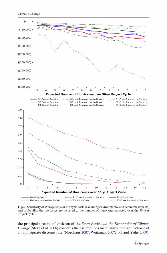
First, Fig. 5 reports the average life cycle costs, excluding environmental and eco-nomic impacts, for the three scenarios including wetland restoration under differentassumptions about the number of hurricanes expected to influence the project area.Figure 5 assumes a wetland storm surge attenuation rate of 1 m:14.5 km, and an 8%discount rate. Although North Carolina may be reasonably expected to receive anaverage of 3–5 hurricanes in a 50-year planning horizon, we show results for a rangeof 3–15 hurricanes over a 50-year planning horizon for extension to other local cases.These results reflect the intuitive idea that the life cycle costs increase as the numberof hurricanes increases. The top panel of Fig. 5 illustrates that under Scenarios 1 and2, utility costs are less than the costs imposed on society through private losses, whilefor Scenario 3, private losses are always less than utility costs. In addition, Fig. 5suggests that private losses under Scenario 3 are most sensitive to increases in thenumber of hurricanes. The bottom panel of Fig. 5 reports the probability that noloss is incurred over the 50-year project life cycle. Although the probability that noloss is incurred decreases substantially for each scenario as the number of hurricanesincreases, the probability that no private loss is incurred remains much higher underScenario 1 than the other Scenarios proposed. For Scenario 1, the probability thatno private losses are sustained remains higher than 0.5 until the number of expectedhurricanes over the 50-year project life cycle increases beyond 10.

5.2.2 Sensitivity to wetland storm surge attenuation rate

On the other hand, our results are much less sensitive to wetland storm surgeattenuation. Figure 6 reports the average life cycle costs, excluding environmentaland economic impacts, for the three scenarios. Figure 6 assumes that five hurricanesare expected to impact the project area over the 50-year life cycle, and that a discountrate of 8% applies. In short, Fig. 6 suggests that life cycle costs for Micropolis are notsensitive to changes in the wetland storm surge attenuation rate over the range ofreported surge attenuation rates. Although utility and private losses are decreasedby approximately 30% over the range of attenuation rates under Scenario 1, theprobability that no costs will be incurred is much less sensitive. This may be dueto the small range between the minimum and maximum storm surge attenuationrates observed. Nonetheless, these results, when considered alongside the literatureinvestigating storm surge attenuation over wetlands, reinforce the importance ofdetailed wetland modeling for local risk analysis and investment planning purposes.While our results show that damages in Micropolis are not sensitive to wetlandstorm surge attenuation rate, Gedan et al. (2010) report that 60% of the variationin damages inflicted on US coastal communities in 34 major hurricanes since 1980 isexplained by differences in coastal wetlands.

5.2.3 Sensitivity to public and private discount rates

The choice of discount rate for evaluating public projects is controversial, especiallywith respect to evaluating climate change mitigation investments. In fact, one of

Climatic Change

Fig. 5 Sensitivity of average 50-year life cycle costs (excluding environmental and economic impacts)and probability that no losses are incurred to the number of hurricanes expected over the 50-yearproject cycle

the principal streams of criticism of the Stern Review on the Economics of ClimateChange (Stern et al. 2006) concerns the assumptions made surrounding the choice ofan appropriate discount rate (Nordhaus 2007; Weitzman 2007; Tol and Yohe 2009).

Climatic Change

Fig. 6 Sensitivity of average 50-year life cycle costs (excluding environmental and economic impacts)and probability that no losses are incurred to the rate of wetland storm surge attenuation

While we do not wish to enter this debate, this discussion indicates the gravity withwhich time preferences must be considered when evaluating private investmentsthat impose considerable public costs and benefits. Consequently, we do consider

Climatic Change

it necessary to discuss the role of the social and private decision makers whenevaluating the potential synergy between wetland restoration and infrastructuredisaster loss mitigation. As indicated, we have assumed a 50-year time horizon forevaluating the electric power hardening investments. This time horizon is symbolicof the difficult negotiation among public and private benefits, as the utility isexpected to develop and manage the infrastructure, while the public must reckonwith the externalities. In addition, this time horizon amplifies the importance of thisnegotiation because this relatively short time horizon implicitly requires that theprivate (utility) decision makers and the public (social/government) decision makersbe represented separately since their benefits accrue on different time scales. For theprivate utility investments and expected costs of repairs and lost revenues, then, weassume an 8% discount rate. This reflects the private utility’s preference to accruebenefits earlier in the project life cycle, as only approximately 2% of the expectedcosts and benefits accrued at the end of the 50-year life cycle are included in thepresent value. On the other hand, the choice of a social discount rate for the costsimposed on society by service interruptions and utility investments is assumed to

Table 7 Sensitivity of average costs for 50-year life cycle of three hardening scenarios to two-decisionmaker scenario, including wetland restoration, and induced economic output and environmentalcosts. (Millions USD) assumes 8% private, 2% social discounting rate

Scenario 1, Scenario 2, Scenario 3,with wetlands with wetlands with wetlands

Maintenance costs $(0.490) $(0.527) $(0.534)Mitigation investment $(138) $(131) $(130)Planned utility costs, C1 $(139) $(132) $(130)Economic output induced $1.461 $1.571 $1.591

by maintenanceEconomic output induced by mitigation $170 $161 $159Environmental costs of maintenance $(13,629) $(14,649) $(14,836)Environmental costs of mitigation $(1,584,700) $(1,500,100) $(1,484,500)Economic value of wetland $1,199 $1,199 $1,199

ecosystem servicesWetland carbon sequestration $1,295 $1,295 $1,295Planned costs imposed on society, C2 $(1,596,000) $(1,512,000) $(1,497,000)Cost of repairs $(0.0148) $(0.0211) $(0.0158)Revenue loss due to disaster $(0.00374) $(0.0298) $(0.0360)Expected utility costs, C3 $(0.0186) $(0.0509) $(0.0518)Economic output induced by repairs $0.0475 $0.0595 $0.0484Lost economic output induced $(0.0166) $(0.107) $(0.152)

by revenue lossDirect private losses $(0.0565) $(0.0714) $(0.0189)Environmental costs of repairs $(442) $(555) $(451)Environmental costs averted s $1,521 $9,828 $13,919

by revenue lossEnvironmental costs averted $0.000454 $0.000574 $0.000151

by private lossesDisaster costs imposed on society, C4 $1,078 $9,273 $13,467Total life cycle costs $(1,594,707) $(1,502,913) $(1,483,394)Average number of hurricanes 3.41 3.51 3.44

in project cycle

Climatic Change

be 2%. This reflects the public’s general unwillingness to bear the costs imposedon them by electric power infrastructure construction, repairs, or failure. An 8%discount rate incorporates approximately 37% of the expected costs and benefitsaccrued to society at the end of the 50-year life cycle are included in the presentvalue. This public–private tradeoff implies that costs over the duration of the projectlife-cycle and beyond should more greatly influence public decision-making whenconsidering electric power infrastructure hardening investments. We report resultsfor this case, including wetland restoration investment, and induced social, economic,and environmental costs, in Table 7. Table 7 shows that, while the environmental andsocial costs and benefits associated with risk mitigation investments take on increasedimportance if a social rate of discounting is assumed, the decision is still dominatedby the price of carbon. We also evaluated 16 pairwise combinations of social discount(0%, 1%, 2%, 3%) and private discount (6%, 8%, 10%, and 12%) rates. Theseresults are not reported here, as the results are not sensitive to changes in thediscount rates over these ranges. Nonetheless, our sensitivity analysis indicates thatthe decision is still dominated by the price of carbon emitted during construction andmaintenance of restored wetlands and electric power network hardening. Thus, whenevaluating risk mitigation and natural restoration decisions, the choice of discountrate may be most important for larger projects, especially if the price of carbon is notincluded.

6 Lessons learned

In summary, our multi-criteria life cycle framework suggests several interestingimplications for future research and planning for wetland restoration projects whenapplied to disaster loss mitigation. Table 8 summarizes the results for each scenariofor each of the three cases examined. For all cases, no infrastructure hardening andno wetland restoration is justified in our case study location. However, we do suggesta few specific areas for additional research:

1. The life cycle analysis must consider non-monetized ecological benefits of wet-land restoration and account for the CO2 production they avert. For example,when considering CO2 emissions in the analysis, the potential for the restoredwetland to become a carbon sink must be evaluated. Even modest amounts ofwetland CO2 sequestration may improve the attractiveness of the project when

Table 8 Summary of the results for each infrastructure hardening scenario for each case

Case: 1 2 3

Wetland restoration: Excluded Included IncludedInduced economic output: Excluded Excluded IncludedEnvironmental impacts: Excluded Excluded IncludedScenario E[NPV] E[NPV] E[NPV]1: Underground all eligible components ($9,294) ($0.0396) ($1,500,000)2: Underground only the commercial district $(1,969) ($0.0280) ($1,418,000)3: No undergrounding ($0.543) ($0.006) ($1,402,000)Preferred alternative Do nothing Do nothing Do nothing

Costs are in million of US dollars

Climatic Change

considered in conjunction with the economic value of the wetlands ecosystemservices and the CO2 emissions averted through ecosystem process production.

2. In the future, simulation of storm surge propagation over constructed or naturalwetlands using more sophisticated models such as SLOSH or ADCIRC may bethe most accurate method of disaster risk assessment. This approach has beenperformed in several of the studies cited here (Loder et al. 2009; Resio andWesterink 2008; Wamsley et al. 2009, 2010), and may more accurately capture theeffects of spatial and temporal heterogeneity in wetland topology, composition,and continuity. Furthermore, storm surge simulation may allow for more flexibleexamination of the influence of factors not yet considered, including wetlandmorphology and wave setup. In addition, because the response of wetlands tostorms, and storm surge to wetlands, may be interactive in nature, stochasticsimulations may be necessary to capture any potential feedback cycles betweenwetland morphology and storm surge attenuation (e.g., consider findings ofWamsley et al. 2009)

3. This work must be replicated using either a larger model city testbed, or atestbed with a different distribution of residential, commercial, and industrialcustomers. This work suggests that the attractiveness of a wetland restorationproject for disaster loss mitigation may be sensitive to the customer mix, althoughwe do not evaluate this sensitivity in this paper. Furthermore, detailed regionaleconomic resilience models should be developed and employed when applyingour framework to a real case. The economic model may become more importantwhen extending the framework to interdependent infrastructures.

4. Although our case study reports that undergrounding and wetland restorationmay increase social costs relative to a completely overhead electric powernetwork configuration, the probability that no social costs are imposed is greatlyincreased under the undergrounding and wetland restoration scenarios proposedin this paper. Future investigation may find this property of electric powernetwork hardening valuable, and should be investigated in conjunction withstorm surge simulation and interdependent infrastructure evaluation.

Overall, our results have important implications for coastal adaptation. Naturalecosystem restoration may be difficult to justify as an approach for coastal adaptationwithout considering the valuation of biodiversity, ecological services, and carbonsequestration. While these issues pose difficult valuation problems, the more directlyquantifiable benefits of wetland restoration may not offset the significant cost ofrestoring or building wetlands in many locations.

Acknowledgements We gratefully acknowledge Drs. Kelly Brumbelow and Alex Sprintson ofTexas A&M University for providing the Micropolis case study, and Dr. Steven Quiring of TexasA&M University for providing the climatic data used in developing the hurricane count model. Wealso acknowledge the funding sources for this work, the National Science Foundation (grant ECCS-0725823), the U.S. Department of Energy (grant BER-FG02-08ER64644) and the Whiting Schoolof Engineering. However, all opinions in this paper are those of the authors and do not necessarilyreflect the views of the sponsors.

References

Arrow KJ, Cropper ML, Eads GC, Hahn RW, Lave LB, Noll RG, Portney PR, Russell M,Schmalensee R, Smith VK, Stavins RN (1996) Is there a role for benefit cost analysis in envi-ronmental, health, and safety regulation? Science 272:221–222

Climatic Change

Bigger JE, Willingham MG, Krimgold F (2009) Consequences of critical infrastructure interdepen-dencies: lessons from the 2004 hurricane season in Florida. Int J Critical Infrastructures 5:199–219

Bridgham SD, Megonigal JP, Keller JK, Bliss NB, Trettin C (2006) The carbon balance of NorthAmerican wetlands. Wetlands 26:889–916

Brown RE (2009) Cost-benefit analysis of the deployment of utility infrastructure upgrades andstorm hardening programs. Quanta Technology, Raleigh

Brumbelow K, Torres J, Guikema SD, Bristow E, Kanta L (2007) Virtual cities for water distrib-ution and infrastructure system research. In Proc. World Environmental and Water ResourcesCongress 2007: Restoring Our Natural Habitat, ASCE/EWRI

Chang SE (2003) Evaluating disaster mitigations: methodology for urban infrastructure systems. NatHazards Rev 4:186–196

Chang SE, Shinozuka M (1996) Life-cycle cost analysis with natural hazard risk. J Infrastruct Syst2:118–126

Chmura GL, Anisfeld SC, Cahoon DR, Lynch JC (2003) Global carbon sequestration in tidal, salinewetland soils. Glob Biogeochem Cycles 17:1111–1123

Costanza R, Farber SC, Maxwell J (1989) Valuation and management of wetland ecosystems. EcolEcon 1:335–361

Costanza R, d’Arge R, de Groot R, Farber S, Grasso M, Hannon B, Limburg K, Naeem S, O’NeillRV, Paruelo J, Raskin RG, Sutton P, van den Belt M (1997) The value of the world’s ecosystemservices and natural capital. Nature 387:253–260

Day JW Jr, Boesch DF, Clairain EJ, Kemp GP, Laska SB, Mitsch WJ, Orth K, Mashriqui H, ReedDJ, Shabman L, Simenstad CA, Streever BJ, Twilley RR, Watson CC, Wells JT, Whigham DF(2007) Restoration of the Mississippi Delta: lessons from Hurricanes Katrina and Rita. Science315:1679–1684

Emanuel K (2005) Increasing destructiveness of tropical cyclones over the past 30 years. Nature436:686–688

Gedan KB, Kirwan ML, Wolanski E, Barbier EB, Silliman BR (2010) The present and future role ofcoastal wetland vegetation in protecting shorelines: answering recent challenges to the paradigm.Clim Change. doi:10.1007/s10584-010-0003-7

Han S-R, Guikema SD, Quiring SM (2009) Improving the predictive accuracy of hurricane poweroutage forecasts using generalized additive models. Risk Anal 29:1143–1153

Hendrickson CT, Lave LB, Matthews HS (2006) Environmental life cycle assessment of goods andservices: an input–output approach. Resources for the Future, Washington, DC

Keeney RL (1982) Decision analysis: an overview. Oper Res 30:803–838LaCommare KH, Eto JH (2006) Cost of power interruptions to electricity consumers in the United

States. Energy 31:1845–1855Loder NM, Irish JL, Cialone MA, Wamsley TV (2009) Sensitivity of hurricane surge

to morphological parameters of coastal wetlands. Estuar Coast Shelf Sci 84(4):625–636.doi:10.1016/j.ecss.2009.07.036

Nicholls RJ, Small C (2002) Improved estimates of coastal population and exposure to hazardsreleased. Eos 83:301–304

Nordhaus WD (2007) A review of the Stern Review on the Economics of Climate Change. J EconLit XLV:686–702

Resio DT, Westerink JJ (2008) Modeling the physics of storm surges. Phys Today 61:33–38Sabbatelli TA, Mann ME (2007) The influence of climate state variables on Atlantic Tropical

Cyclone occurrence rates. J Geophys Res 112:D17114. doi:10.129/2007JD008385Small C, Nicholls RJ (2003) A global analysis of human settlement in coastal zones. J Coast Res

19:584–599Stern N, Peters S, Bakhshi V, Bowen A, Cameron C, Catovsky S, Crane D, Cruickshank S, Dietz S,

Edmonson N, Garbett S-L, Hamid L, Hoffman G, Ingram D, Jones B, Patmore N, Radcliffe H,Sathiyarajah R, Stock M, Taylor C, Vernon T, Wanjie H, Zenghelis D (2006) The economics ofclimate change. HM Treasury, London

The European Climate Exchange (2009). http://www.ecx.eu. Accessed 15 February 2010The Green Design Institute (2009) Economic input–output life cycle analysis model (EIO-LCA).

Carnegie Mellon University, Pittsburgh, PA. http://www.eiolca.netTol RSJ, Yohe GW (2009) The Stern Review: a deconstruction. Energy Policy 37:1032–1040Turner RE, Streever BJ (2006) Approaches to coastal wetland restoration: Northern Gulf of Mexico.

SPB Academic Publishing, The HagueU.S. Army Corps of Engineers, New Orleans District (1963) Interim survey report, Morgan City, LA

and vicinity. New Orleans, LA

Climatic Change

U.S. Army Corps of Engineers, New Orleans District (2004) Louisiana coastal area ecosystemrestoration study. New Orleans, LA

U.S. Congress Office of Technology Assessment (1990) Physical vulnerability of electric systems tonatural disasters and sabotage, OTA-E-453, U.S. Government Printing Office, Washington, DC

Wamsley TV, Cialone MA, Smith JM, Ebersole BA, Grzegorzewski AS (2009) Influence of land-scape restoration and degradation on storm surge and waves in southern Louisiana. Nat Hazards51:207–224

Wamsley TV, Cialone MA, Smith JM, Atkinson JH, Rosati JD (2010) The potential of wetlands inreducing storm surge. Ocean Eng 37(1):59–68. doi:10.1016/j.oceaneng.2009.07.018

Weitzman ML (2007) A review of the Stern Review on the Economics of Climate Change. J EconLit XLV:703–724

Xu L, Brown RE (2008) Undergrounding assessment Phas 3 Report: Ex Ante Cost and BenefitModeling. Quanta Technology, Raleigh