Assessing the temporal variability in extreme storm-tide time-series for

coastal flood risk assessment

N. Quinn1,*, M. Lewis2, M. P. Wadey3, I.D. Haigh3

1School of Geographical Sciences, University of Bristol, University Road, Bristol, BS8 1SS, UK.

2School of Ocean Sciences, Bangor University, Menai Bridge, LL59 5AB, UK.

3Ocean and Earth Science, National Oceanography Centre, European Way, Southampton SO14 3ZH,

UK.

*Corresponding author. Tel.: +44 1179288290; E-mail address: Niall.Quinn@Bristol.ac.uk (N. Quinn)

Key Points:

Extreme storm tide time-series variability is examined along the UK coastline

Variability is shaped by site location and time relative to high water

Time-series uncertainty can have significant impacts on flood risk predictions

Journal of Geophysical Research – Oceans May 2014

Research Article Journal of Geophysical Research: Oceans DOI 10.1002/2014JC010197

This article has been accepted for publication and undergone full peer review but has not beenthrough the copyediting, typesetting, pagination and proofreading process which may lead todifferences between this version and the Version of Record. Please cite this article asdoi: 10.1002/2014JC010197

© 2014 American Geophysical UnionReceived: May 30, 2014; Revised: Jul 15, 2014; Accepted: Jul 16, 2014

2

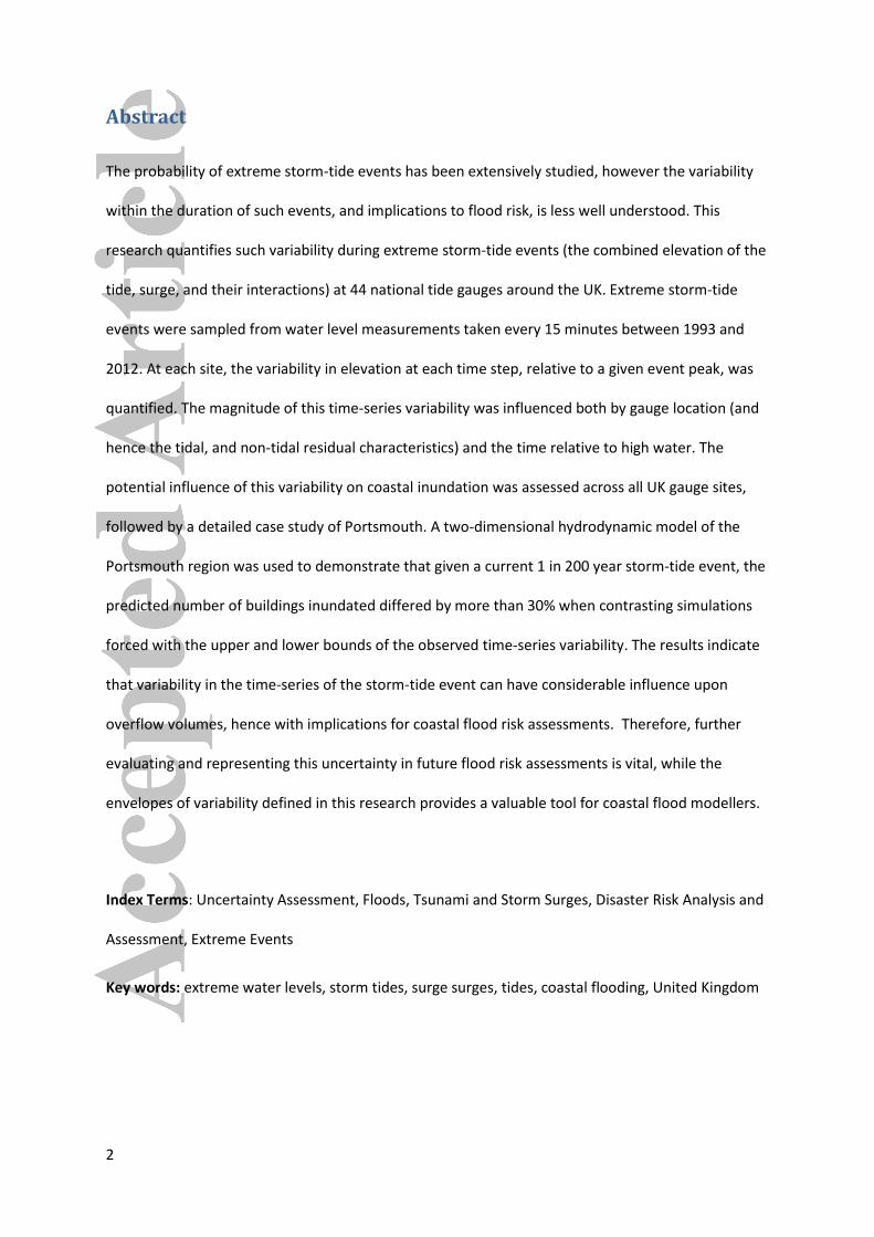
Abstract

The probability of extreme storm-tide events has been extensively studied, however the variability

within the duration of such events, and implications to flood risk, is less well understood. This

research quantifies such variability during extreme storm-tide events (the combined elevation of the

tide, surge, and their interactions) at 44 national tide gauges around the UK. Extreme storm-tide

events were sampled from water level measurements taken every 15 minutes between 1993 and

2012. At each site, the variability in elevation at each time step, relative to a given event peak, was

quantified. The magnitude of this time-series variability was influenced both by gauge location (and

hence the tidal, and non-tidal residual characteristics) and the time relative to high water. The

potential influence of this variability on coastal inundation was assessed across all UK gauge sites,

followed by a detailed case study of Portsmouth. A two-dimensional hydrodynamic model of the

Portsmouth region was used to demonstrate that given a current 1 in 200 year storm-tide event, the

predicted number of buildings inundated differed by more than 30% when contrasting simulations

forced with the upper and lower bounds of the observed time-series variability. The results indicate

that variability in the time-series of the storm-tide event can have considerable influence upon

overflow volumes, hence with implications for coastal flood risk assessments. Therefore, further

evaluating and representing this uncertainty in future flood risk assessments is vital, while the

envelopes of variability defined in this research provides a valuable tool for coastal flood modellers.

Index Terms: Uncertainty Assessment, Floods, Tsunami and Storm Surges, Disaster Risk Analysis and

Assessment, Extreme Events

Key words: extreme water levels, storm tides, surge surges, tides, coastal flooding, United Kingdom

3

1. Introduction

Coastal areas are heavily populated regions throughout the world; more than a billion people and a

significant portion of the global gross domestic product (GDP) are found within 100 km of the coast

(Small and Nicholls, 2003). Over recent decades, coastal populations have continued to grow much

more rapidly than global mean populations, particularly in less developed countries (Spencer and

French, 1993; Hunt, 2005). Continued urbanisation and migration is expected to significantly

increase the value of assets found near coasts in the coming century (Nicholls, 1995; Turner et al.,

1996; Zong and Tooley, 2003; Mokrech et al., 2012). Given that 14 out of the world’s 17 recognised

global megacities (with populations exceeding 10 million) are located in coastal zones (Tibbetts,

2002; Sekovski et al., 2012); accurately assessing flood risk to these densely populated regions is of

critical importance for coastal communities and to guide adaption strategies.

Storm-tides are the total still (i.e. excluding waves) water-levels experienced at the coast due to the

combination of three main factors: (1) mean sea-level; (2) astronomical tide; and (3) storm surge

(Pugh, 2004; Lewis et al., 2011); and can result in devastating coastal floods due to the large number

of people and assets in low lying coastal regions found throughout the world. For example, more

than 440,000 people were killed in two storm-tide events occurring in 1970 and 1991 in the Bay of

Bengal alone (Flather, 1994), while Hurricane Katrina (e.g. RMS, 2005) and Hurricane Sandy have

recently caused devastation on the US coastline. More recently, Typhoon Haiyan, which hit the

Philippines in November 2013, induced a storm tide of more than 25 feet (7.6 m) which affected

more than 14 million people, causing about 6,200 deaths (Barmania, 2014; see also

http://reliefweb.int/disaster/tc-2013-000139-phl for more information).

Efficient planning and resource allocation is essential in order to cope with current risk, and the

likely increase in risk facing many areas due to rising mean sea levels in the coming century

(Houghton, 2005; Meehl et al., 2007; Lowe et al., 2009; Haigh et al., 2011). Furthermore, due to the

temporal lead time required to construct mitigation strategies and flood defences, an accurate

4

assessment of the spatial and temporal changes to risk (here defined as the product of the

probability and consequences of flooding) is vital and imminently required. An important component

of this process is accurate risk-based assessments to inform policy decisions. Typically this is

achieved using a numerical modelling approach in which storm-tide conditions of interest,

commonly based on a probability of exceedence or ‘return period’ (e.g. Tawn, 1992; Haigh et al.,

2010), are imposed upon an inundation model domain boundary (e.g. Bates et al., 2005; Bates et al.,

2010), which may incorporate defence responses and be used to assess economic damage (e.g.

Dawson et al, 2009). Resulting flood conditions may be used to infer likely inundation extents and

potential losses for specific flood events (e.g. Stansby et al., 2012; Smith et al., 2012; Wadey et al.,

2012). These assessments provide a vital tool for informing policy decisions (e.g. cost-benefit of

flood defences; shoreline planning) and scenario-based assessment of coastal change (Dawson et al.,

2003). However, errors are inevitably introduced into model predictions through a variety of sources

including inaccurate estimates of initial conditions, inaccurate boundary forcing, and lack of

complete knowledge of the system leading to an inability of numerical models to fully represent

many physical processes (Maybeck, 1979; Madsen and Canizares, 1999; Kantha and Clayson, 2000;

Brown et al., 2007; Neal, 2007). Such uncertainties will impact both deterministic and probabilistic

predictions of inundation extent and depth. The ultimate result is divergence from reality in the

model predictions. Understanding this uncertainty is essential as unrealistic expectations of

accuracy can result in the misinterpretations of flood risk, with profound implications (Brown and

Damery, 2002; Hall and Solomatine, 2008). For this reason, many operational forecasting systems

and risk assessments provide probabilistic predictions in an attempt to explicitly account for known

uncertainties in the modelling approach used (e.g. Purvis et al., 2008; Bocquet et al., 2009;

Pappenberger et al., 2006; Davis et al., 2010; Kim et al., 2010).

A fundamental source of uncertainty in various coastal-based numerical models and empirical

approaches used to predict coastal events and change (e.g. flooding, sediment transport and

erosion), is the specification of the tide and surge boundary conditions. Model sensitivity due to this

5

input is high, due to its fundamental influence upon the volume and rate at which water enters the

model domain (and can then be distributed). It has been established that astronomical tidal

elevations are often not predicted well by physically-based numerical models (particularly in

complex nearshore regions) hence harmonic tide predictions (based on measured data) are

substituted in the place of outputs from such models in many operational systems due to their

greater accuracy (Bocquet et al., 2009; Flowerdew et al., 2009). Furthermore meteorically induced

storm surges, tide-surge interaction effects causing phase variation, and local conditions (e.g.

bathymetry) complicate combined tide and surge predictions (which we call storm-tide). Recently,

progress has been made in forecasting extreme storm-tides around complex coastlines allowing for

more accurate estimates between gauged locations (Horsburgh et al., 2008; Lewis et al., 2011; 2013)

and in the prediction of the heights and probabilities of extreme sea levels (McMillan et al., 2011;

Batstone et al., 2013; Haigh et al., 2014a,b).

Typically an idealised storm-tide time-series (often derived from a previously observed event) is

applied to these return level estimates to force an inundation model at a given location (e.g.,

Dawson et al., 2005a; Purvis et al., 2008; McMillan et al., 2011; Batstone et al., 2013; Gallien et al.,

2011; Quinn et al., 2013). However, the true storm-tide time-series is likely to vary spatially (along a

section of coastline) and temporally (between subsequent events), even for a given event

magnitude, due to variability in tide and surge characteristics, and the complexity of their

interactions (Horsburgh and Wilson, 2007; Wolf, 2009; Brown et al., 2011; Lewis et al., 2013). No

two storm-tide events are the same, because different combinations of tide and surge

(superimposed on different mean sea levels) combine to give the total water levels observed during

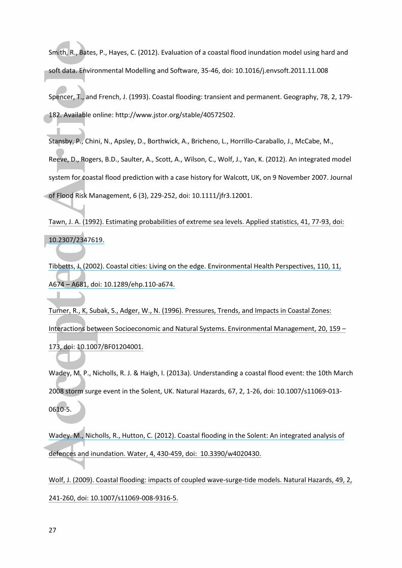
events. For example, Fig. 1 shows time-series of total water level at Liverpool for 8 events, and the

corresponding time-series of tide and non-tidal residual that combine to give the total water levels

for those 8 events. The non-tidal residual is the difference in elevations relative to those generated

by the tide alone and primarily contains the surge and tide-surge interaction effects (Pugh, 1987;

Horsburgh and Wilson, 2007). For each of the 8 events, the maximum water level is 10.37 m Chart

6

Datum (which corresponds to a 1 in 2 year return period). But what is clear from Fig. 1 is that the

temporal variability in the hours leading up to and then proceeding the peak water level of each of

these 8 events is different, because of differences in the tidal and non-tidal residual time-series. This

uncertainty in the storm-tide time-series is not commonly quantified in coastal flood risk

assessments, and hence is the focus of our study.

Uncertainty in the true time-series of a storm-tide event, particularly close to the time of high water

(when defence exceedance is most likely) may lead to uncertainty in the duration (and therefore

volume) of water affecting a region of interest; a factor currently not considered systematically in

many flood risk assessments. This will have important implications on the simulated inundation

extent and depth, and thus the predicted risk. Further, the probability of defence failure is likely to

increase the longer a peak water-level persists, while other processes of relevance to flood risk such

as wave-overtopping and erosion of beaches and soft defences would also be expected to respond

to changes in the storm-tide time-series (e.g. Pullen et al., 2007; Roelvink et al., 2009).

Therefore, the first objective of this paper is to define the uncertainty within such an assumption by

quantifying the natural observed variability in extreme storm-tide time-series around the UK; a

region that has a long history of coastal flooding, particularly from surges occurring in the North Sea

(e.g. Gönnert et al., 2001; McRobie et al., 2005; Baxter et al., 2005; Gerritsen, 2005). Most recently,

throughout December 2013 to February 2014, many areas of the UK experienced a sequence of

severe storm events, leading to thousands of homes being flooded and many more evacuated

(Slingo et al., 2014). This information will be useful to better inform future flood risk assessments.

The magnitude of the variability in storm-tide time-series is assessed around the UK in order to

ascertain site characteristics that are prone to induce a high level of uncertainty in an extreme

storm-tide time-series; information that will be of value to policy makers and modellers interested in

coastal flood risk. The second objective of the paper is to examine the implications of the variability

observed in the storm-tide time-series at different sites. We do this by undertaking a theoretical

assessment of overflow volumes (where still water levels exceed defence elevations) at each gauge

7

site, and also carry out a case study sensitivity analysis of flood inundation at Portsmouth, one of the

most flood prone cities in the UK.

The paper is formatted as follows: Section 2 introduces the study sites and datasets; Section 3

describes the methods used to define the variability in storm-tide time-series and examine its

significance to flood risk; the results and discussion are presented in Section 4; while the conclusions

are given in Section 5.

2. Sea level datasets

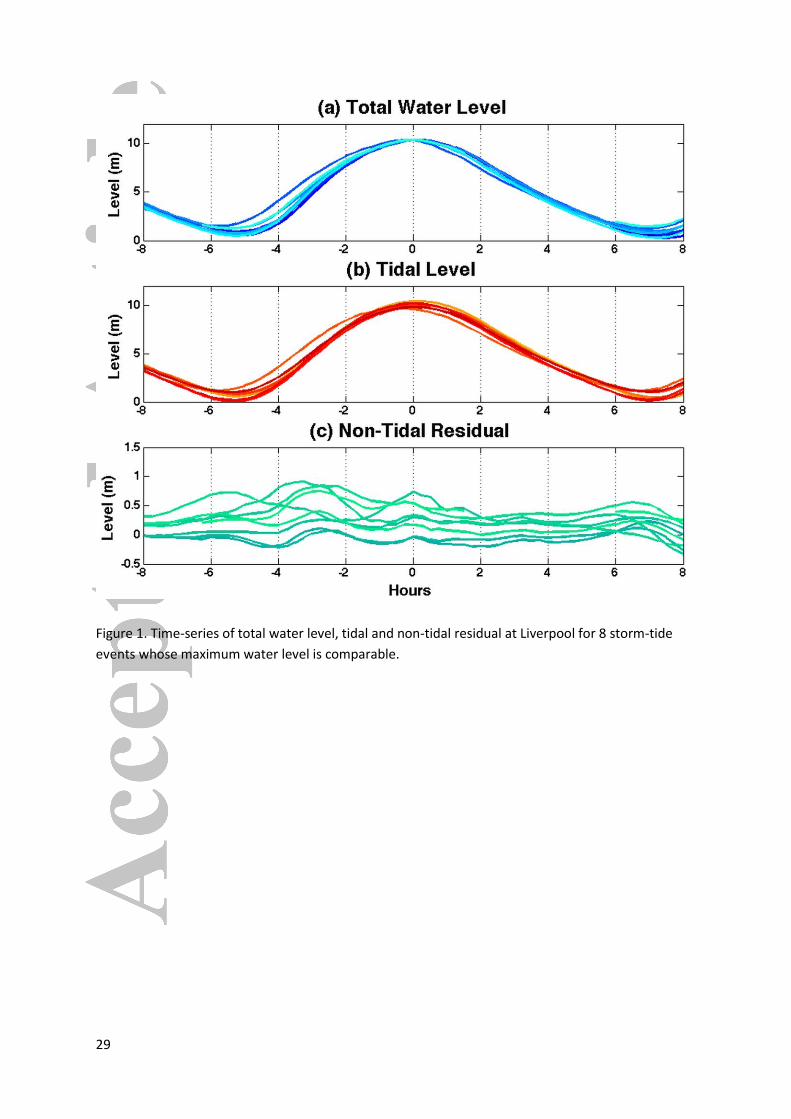
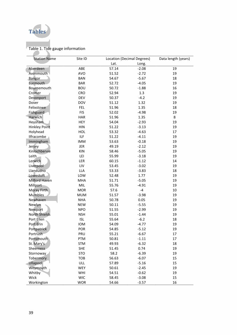
This research focussed on water level time-series measured across the comprehensive UK national

A-Class tide gauge database (Fig. 2 and Table 1). Water level measurements at 15 minute temporal

resolution were obtained for 44 sites around the UK from the British Oceanographic Data Centre

(BODC, www.bodc.ac.uk), who archive and quality control the data on behalf of the National Tidal

and Sea Level Facility (www.ntslf.org). To ensure results were comparable between sites, the focus

was only on the 20-year period from 1993-2012. All sites contained at least 15 years of data for this

period with the exception of Harwick, Lerwick and Moray Firth, which included 8, 14 and 10 years,

respectively. All data archived by the BODC has undergone quality control and corresponding quality

markers are recorded, which were used to remove any potentially erroneous data prior to analysis.

As the focus is on comparing extreme storm-tides, we removed the mean sea level component from

the measured water level datasets and then separated the time-series into an astronomical tidal

component and a non-tidal residual. To isolate the contribution of sea level changes caused by

individual storm events (rather than longer term seasonal or inter-annual changes in meteorology),

the MSL component (indicative of seasonal, inter-annual and longer-term change) was derived using

a 30-day running mean of the observed sea level time-series at each site, and this was subsequently

removed from the record for that site. Harmonic analysis was performed with T-Tide (Pawlowicz et

al., 2002) for each calendar year with the standard set of 67 tidal constituents, to predict the tidal

8

component. The non-tidal residual was determined by subtracting the calculated tidal component

from the measured time-series.

3. Methods

3.1. Variability in the storm-tide event time-series

The first study objective is to quantify the variability during extreme storm-tide event time-series,

particularly in the hours leading up to and then proceeding the peak water level of events. To do this

a representative set of extreme storm-tide event time-series was selected from the available data at

each site. Using this selected ensemble of events, the spread (variability) in the water level

elevations, every 15 minutes, over a 12 hour event time window, centred on time of maximum

water level, was examined and used to define a representative mean, upper and lower storm-tide

time-series, which captures the envelope of variability at each site.

Preliminary analysis indicated that the data selection criterion was influential upon the resulting

ensemble, and therefore, the estimate of time-series variability. Relaxing the high water constraint

(thereby including a greater number of events) at a site was found to result in a larger spread in the

ensemble at any given time step. As this research was primarily interested in quantifying the

variability in extreme storm-tide time-series and its potential impacts on flood risk, only the largest

1% of events was used at each site. This enabled the research to focus on defining the time-series

variability in the largest events, which will be of most interest to flood risk managers, while allowing

for adequately large ensembles (between 100 – 150 events) to still be considered at each site.

The following steps were used at each site shown in Fig. 2:

a) Every high water was identified from the available data, and all but the largest 1% were

discarded;

9

b) The remaining high water points were used as index points to extract the total water

level, tide, and non-tidal residual elevations 6 hours either side of the peak, at 15 minute

resolution;

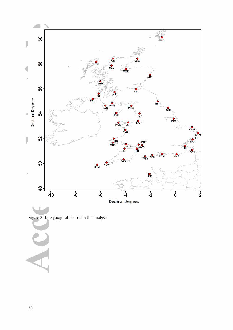
c) Considering the ensemble of time-series; the standard deviation, mean, 95th and 5th

percentile statistics at each time step were then calculated;

d) For each event, the water level at each time step was calculated as a proportion of the

event peak to allow comparison of the time-series shape between events more easily. The

same statistics calculated in step c) were then extracted from the new normalised ensemble

of time-series.

The standard deviation in the tide, non-tidal residuals, and total water level ensembles at each time

step were used as a primary indicator of variability of the storm-tide time-series; representing the

spread in elevations at a time step, given as a proportion of the event peak magnitude. The

ensemble mean, 95th and 5th percentile time-series provided the upper and lower bounds on the

likely shape of an extreme storm-tide time-series at a given site (Fig. 3).

3.2. Influence of time-series uncertainty on coastal inundation

The second objective of the paper is to examine some of the implications of the variability in the

storm-tide time-series defined in objective 1. To do this, two sets of analysis were made: a

theoretical assessment of overflow volumes at each site; and a detailed local analysis of the impact

on flooding inundation extent at Portsmouth.

To examine the potential implications upon defence overflow volumes at the gauge sites, the peak

storm-tide heights with a 1 in 300, 500, and 1000 year probability of exceedance were selected

(estimated by McMillan et al., 2011 for the UK Environment Agency), and the uncertainty associated

with the water-level time-series of these events investigated. The upper and lower bounds of the

10

variability envelopes defined in Section 3.1 (Fig. 3) were used to define two event time-series for

each of the selected event magnitudes, at each site.

At each site, a hypothetical sea defence built to a 1 in 200 year level standard was defined (the

standard for approximately 400,000 homes in the UK coastal zone; Committee on Climate Change,

2013) and the constructed storm-tide time-series were used to estimate overflow volumes during

the event. The flow of water over the defence was represented by broad crested weir equations

(Ackers et al., 1978; Quinn et al., 2013). Given these conditions, the volume of discharge (per unit

length of defence) was calculated every 15 minutes, and the total event discharge was given as the

sum of all time steps. In this example, the water level in a given bin was assumed to be static for the

15 minute duration of the bin. The total event discharge can be represented by:

∑

where QT is the total event discharge, and the discharge in bin i, Qi, is given by

where C is a weir coefficient (given as 1.5), L is the length (1 m), and H is the water head (m).

Four sites away from Mainland UK (Bangor, Harwich, Saint Helier and Portrush) were not included in

this portion of the analysis because return period statistics were not available for them (McMillan et

al., 2011; Batstone et al., 2013).

To provide a more detailed example of the potential impacts of time-series variability upon extreme

events, a two-dimensional (2D) inundation case study was also undertaken for the low lying and

densely populated UK city of Portsmouth which is ranked only behind London and Hull for the

amount of property at risk of coastal flooding (RIBA and ICE, 2009). The city is surrounded by hard

defence structures, most of which are expected to provide approximately a 1 in 200 year standard of

protection. The flood simulation method comprised point vectors placed onto the edge of a digital

elevation model (DEM), with each point associated with a storm tide water level time-series. The

11

DEM was assembled from LiDAR data collected between 2007 and 2008 by the Environment Agency

(EA) at 1-2m resolution. This was spatially averaged to 50 m cells. For the case study of Portsmouth

this resulted in 150 columns and 168 rows of cells, in the form of a regular grid. The vertical root

mean square error of the LiDAR collected by the EA was within ± 0.10 m of the available ground-

based check-points. Flood water was propagated inland using the 2D raster based inundation model

LISFLOOD-FP (refer to Bates et al., 2010 for technical details of this model). The coarse scale is

acknowledged in this example for urban flood modelling: finer resolution grids can generate more

accurate representations of flow diverting around buildings, whilst less interpolation of the original

topographic survey data can allow a more realistic approximation of floodplain water depths

(Fewtrell et al., 2008). However, the modelling method has been validated against real floods in

nearby areas (Wadey et al., 2012; Wadey et al., 2013a) and is hence considered to be sufficient to

demonstrate the effects of different storm-tides on basic coastal flood predictions. Two defence

conditions scenarios were simulated:

1) No breach – defence crest heights collected by ground-based surveys with ± 0.03 m

accuracy were appended to the DEM. The storm tide water level time-series was routed

over these defences which were assumed to hold.

2) Breach – defence structures were removed from the DEM and water was able to flow into

the domain if the land height behind the defence was lower than the inflow boundary water

level. Although breaching is unlikely to occur in such a drastic manner, agencies such as the

EA often define flood maps under such conditions (e.g. http://apps.environment-

agency.gov.uk/wiyby/37837.aspx).

Wave-overtopping was excluded due to the high uncertainties described in previous studies,

especially when linked to inundation simulations (e.g. Pullen et al., 2007;Pullen et al., 2009; Smith et

al., 2012) although more recent research has reported prediction accuracies of approximately 20%

when compared to field data (McCabe et al., 2013). Furthermore Portsmouth has not experienced a

12

major coastal flood in recent years, and it was not possible to calibrate the wave-overtopping

predictions. Surface friction, parameterized within the LISFLOOD-FP kinematic wave equation as the

Manning’s n roughness coefficient (see Bates et al., 2010), was set at a spatially homogenous value

of 0.035, while the time-step was set within the model to optimise stability and computational

efficiency.

Water level peaks representing 1 in 1, 10, 50, 200, 300, 500, and 1000 year events were calculated

for the Portsmouth tide gauge. For each event peak, 2 time-series were created using the upper and

lower storm-tide time-series bounds for the Portsmouth site, defined in the analysis outlined in

Section 3.1. Each event time-series was used as a water level boundary condition to force the

inundation model for both the breach and no breach scenarios. The resulting inundation and

property damages were then contrasted.

4. Results and discussion

4.1. Variability in the storm-tide event time-series

Using the methods described in Section 3.1, the variability in the measured storm-tide time-series,

tide, and non-tidal components, was examined at each study site. Given the ensemble of events

examined and the statistics extracted (Section 3.1), variability was found in the tide and non-tidal

residual time-series ensembles, and therefore, the resulting storm-tide time-series, at each time

step.

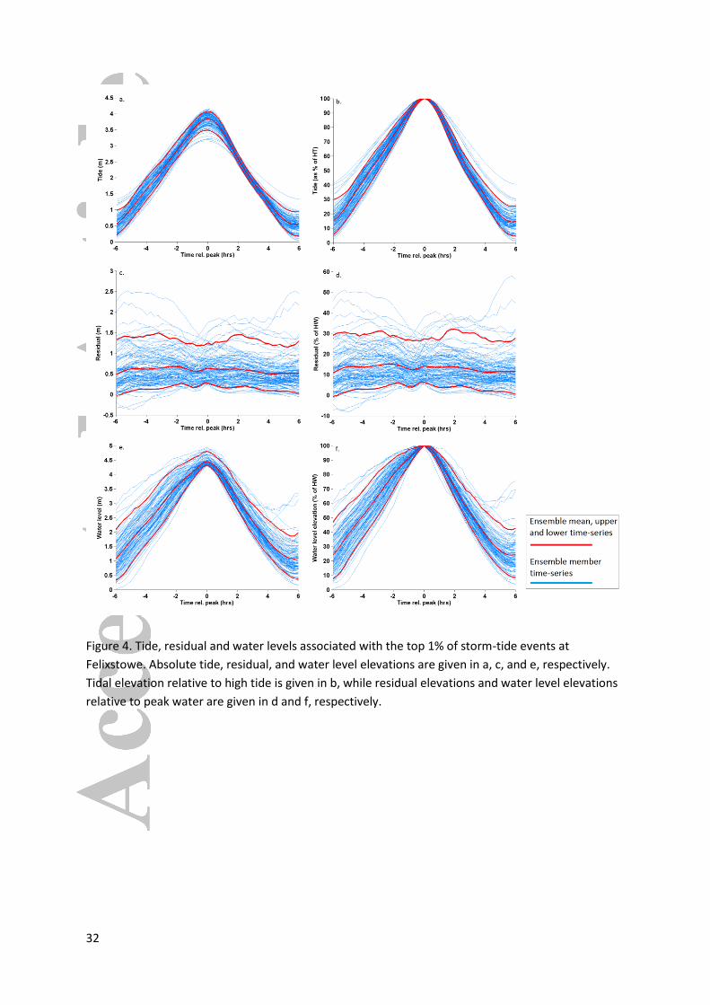
Using Felixstowe as an illustration, Fig.4 (a, b) show the tidal time-series ensembles, and the tidal

time-series ensembles where elevation is normalised relative to the high tide magnitudes,

respectively. Fig.4 (c, d) show the non-tidal residual time-series ensembles, and the residual time-

series ensembles where elevation is normalised relative to the high water magnitudes, respectively.

The variability in the time-series of these signals, when comparing the ensembles of events, led to

13

significant variability in the ensemble of the storm-tide time-series at the tide gauges considered in

this research (Fig.4 e, f). Previous research (e.g. McMillan et al., 2011; Batstone et al., 2013) has also

demonstrated that the magnitude of non-tidal residuals at a given time relative to high water can

differ considerably between events, with important implications upon the resulting storm-tide time-

series.

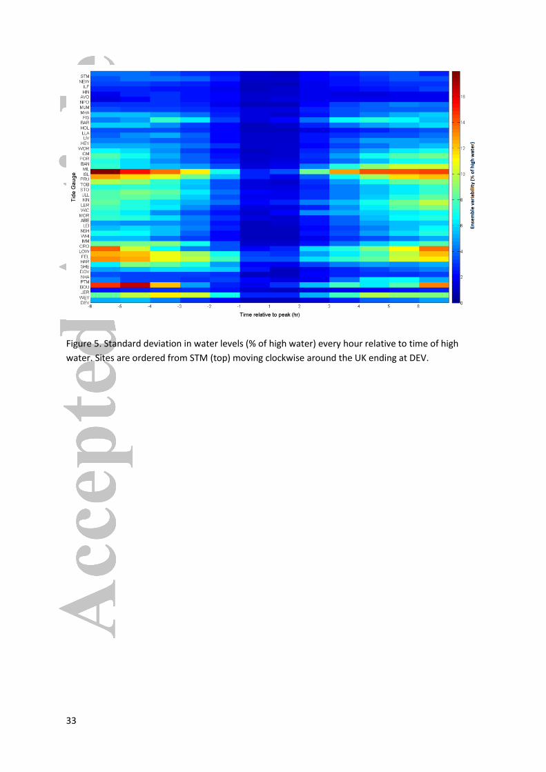
The time-series variability at each site (defined by the standard deviation in the storm-tide elevation

ensemble, every hour relative to the high water) is shown in Fig. 5, while the event-mean (mean of

all time steps) is plotted in Fig. 6 for each site. The magnitude of the variability in the storm-tide

time-series ensemble at a given site varied with the time relative to high water, with an r2

correlation of 0.98 when plotting the mean variability at each time step across all sites against the

time from high water. This finding indicates that close to high water, variability in the time-series

between events is relatively low (e.g. commonly less than 1.5% and less than 3.6% within 1 hour at

all sites). Examination of the tidal time-series ensembles at each site indicated that time-series

variability in tidal elevations, relative to the high water, increased away from high water (Fig. 4 a, b).

This demonstrates that although the tide can be considered as relatively predictable, the time-series

of tidal cycles within the ensemble of events considered in this research will vary depending on the

magnitude of the high tide. Furthermore, interactions between tides and surges have been shown to

alter the wave phase speeds of both signals, often resulting in the clustering of non-tidal residual

peaks away from high water (Horsburgh and Wilson, 2007; Howard et al., 2010). This will be of

particular importance to those interested in flood risk due to wave-overtopping and overflow of

defences, both of which are most likely to occur near to high water, and therefore, this portion of

the storm-tide time-series (and its uncertainty) will be of greatest importance to predictions of

inundation depth and extent.

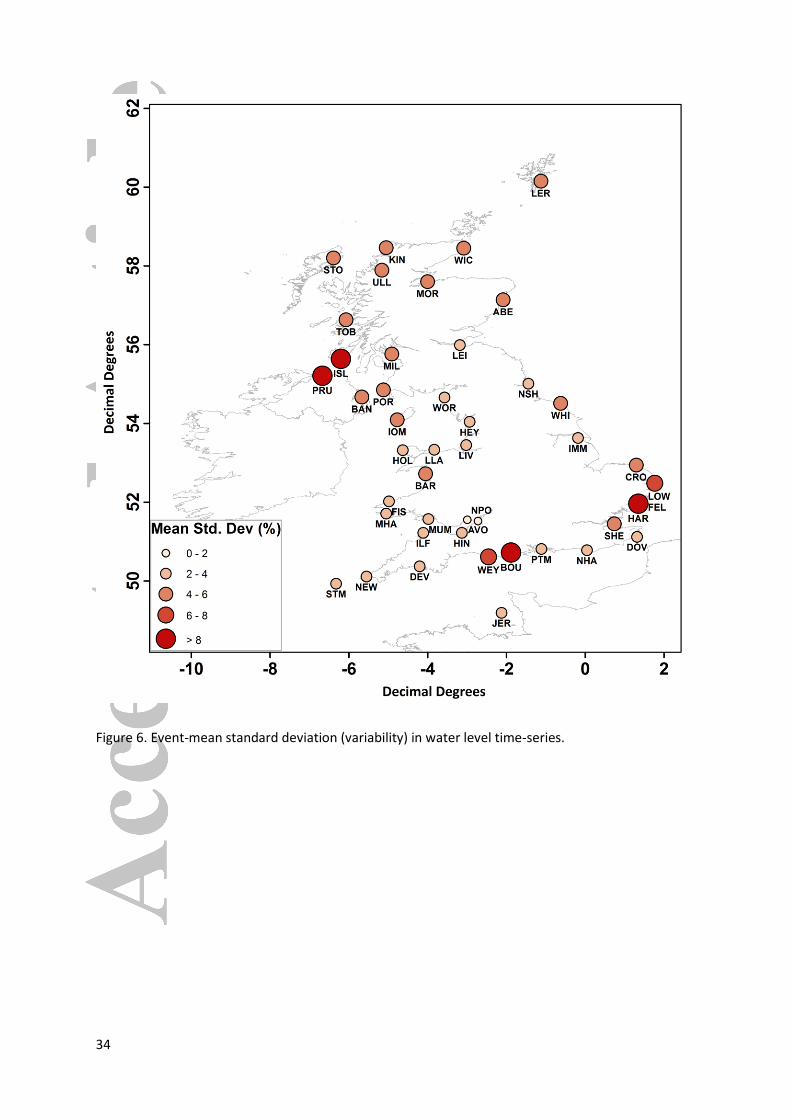
Comparison of the results at all UK gauges revealed that the magnitude of the variability in the

storm-tide time-series ensemble also differed significantly between sites. Given the event-mean

variability in the water levels (the mean of all time steps) at each site (Fig. 6), the results indicate

14

that the magnitude of the variability in storm-tide time-series across the UK ranged from 1.9% at

Newport to 11.3% at Port Ellen, with a UK mean of 4.6%. Using Fig. 6, regional characterisations can

be made. For instance, the greatest mean variability in water level time-series, when considered as a

proportion of high water, was found in the northwest at sites such as Port Ellen and Portrush, and in

the southeast at Harwich and Felixstowe. Alternatively, the southwest was shown to contain the

least variability, the reasons for which are discussed below.

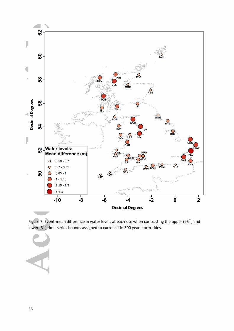
For context, given a 1 in 300 year event peak magnitude, the event-mean difference between the

upper (95th) and lower (5th) bounds of the time-series variability across all sites, in meters, was 0.95

m, with the largest and smallest differences occurring at Felixstowe (1.56 m) and Lerwick (0.59 m),

respectively (Fig. 7). Where only the high water (+/- 3 hours) of the time-series was considered, all

sites lay within 2 standard deviations of the UK mean, given as 0.17 m and 0.65 m respectively, with

the exception of Felixstowe, which had a larger mean difference between the two time-series

bounds than expected (1.1 m). All sites assessed showed a difference of at least 0.4 m between the

upper and lower time-series bounds within 3 hours of high water.

The considerable differences in time-series variability between the gauge sites are due to the

differing tide and non-tidal residual characteristics found around the UK (see Pugh, 1987). For

instance, plotting the event-mean time-series variability against the ensemble mean tidal range at

each site provided an r2 correlation of 0.78 (Fig. 8). This relationship was not unexpected given that

in this research variability was normalised by the corresponding high water magnitude.

The magnitudes of the non-tidal residuals at a site were also influential to the time-series variability

when considered in addition to the tidal range. The magnitude of the 99th percentile non-tidal

residual was found for each site and normalised by the corresponding ensemble mean tidal range.

Plotting this new variable against the event-mean variability in the storm-tide ensembles at each site

provided an r2 correlation of 0.86 (Fig.8). This plot indicates that sites with relatively low tidal ranges

and large non-tidal residual magnitudes are likely to contain the greatest variability in the storm-tide

15

time-series when given as a proportion of the storm-tide peak elevation. Although small errors in the

calculated non-tidal residual may be present (see Horsburgh and Wilson, 2007), it is expected the

99th percentile magnitude used here is a suitable indicator of the difference in the non-tidal

component of the water levels between sites.

This correlation helps to explain why within the Severn Estuary the ensemble with the least

variability in the ensemble of event time-series was found. At Avonmouth, for example, although the

99th percentile non-tidal residual magnitude was the largest of all the sites, the extremely large tidal

range (exceeding 13 m) resulted in one of the smallest non-tidal residual: tidal range ratios, and

subsequently, one of the lowest scores for storm-tide time-series variability. The opposite was found

at sites such as Lowestoft and Port Ellen, where some of the smallest tidal ranges (due to their

proximity to amphidromic points) coincided with relatively large 99th percentile non-tidal residual

magnitudes.

These findings demonstrate that when considering the largest 1% of events, there is variability in the

time-series of extreme storm-tides recorded at all Class A tide gauges around the UK. The results

presented also provide a valuable insight into how the magnitude of this variability changes spatially

between tide gauge sites and temporally during an event. The envelopes of variability calculated at

each site could be used in future probabilistic flood risk assessments to more accurately quantify the

uncertainty in the model outputs due to assumptions commonly made about the time-series of the

storm-tide boundary conditions; currently not considered in most coastal flood risk studies. For

instance, given a 1 in 300 year event peak magnitude at a given site, the upper and lower event

time-series bounds defined in this research could be used as boundary conditions to an inundation

model. By simulating the model with both sets of boundary conditions, the uncertainty in the

prediction of coastal inundation due to uncertainty in an extreme event time-series could be

properly quantified. By describing these idealised time-series as a proportion of the high water, the

envelopes of variability defined may be applied to any given return period event of interest.

16

4.2. The potential impact upon coastal inundation

The potential impacts of the variability discussed in Section 4.1 upon coastal inundation predictions

were examined using the methods and variability envelopes described in Section 3.2. Given the

differences in the storm-tide time-series upper and lower bounds for the events described in Section

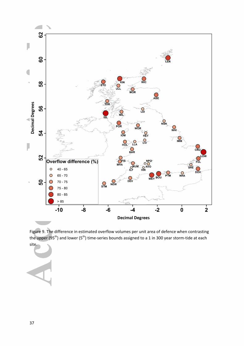
3.2, the idealised defence overflow analysis (shown in Fig. 9) indicated that there was considerable

uncertainty in the predicted overflow volumes during an extreme event. Given a 1 in 300 year storm-

tide event, the difference between overflow volumes estimated using the upper and lower bound

time-series ranged from 63% (Port Ellen) to 88% (Lowestoft), with a UK mean of 73%. The same

analysis, considering 1 in 500 and 1 in 1000 year events indicated that the greatest uncertainty is

likely to be during less severe events, for instance, where overflow of defences occurs for a relatively

short duration, due to the proportional assessment used. However, even during very extreme events

the difference in predicted overflow volumes remained high. For instance, the mean difference in

overflow volumes (given all sites) was 69% and 47% for the 1 in 500 and 1 in 1000 year events

respectively.

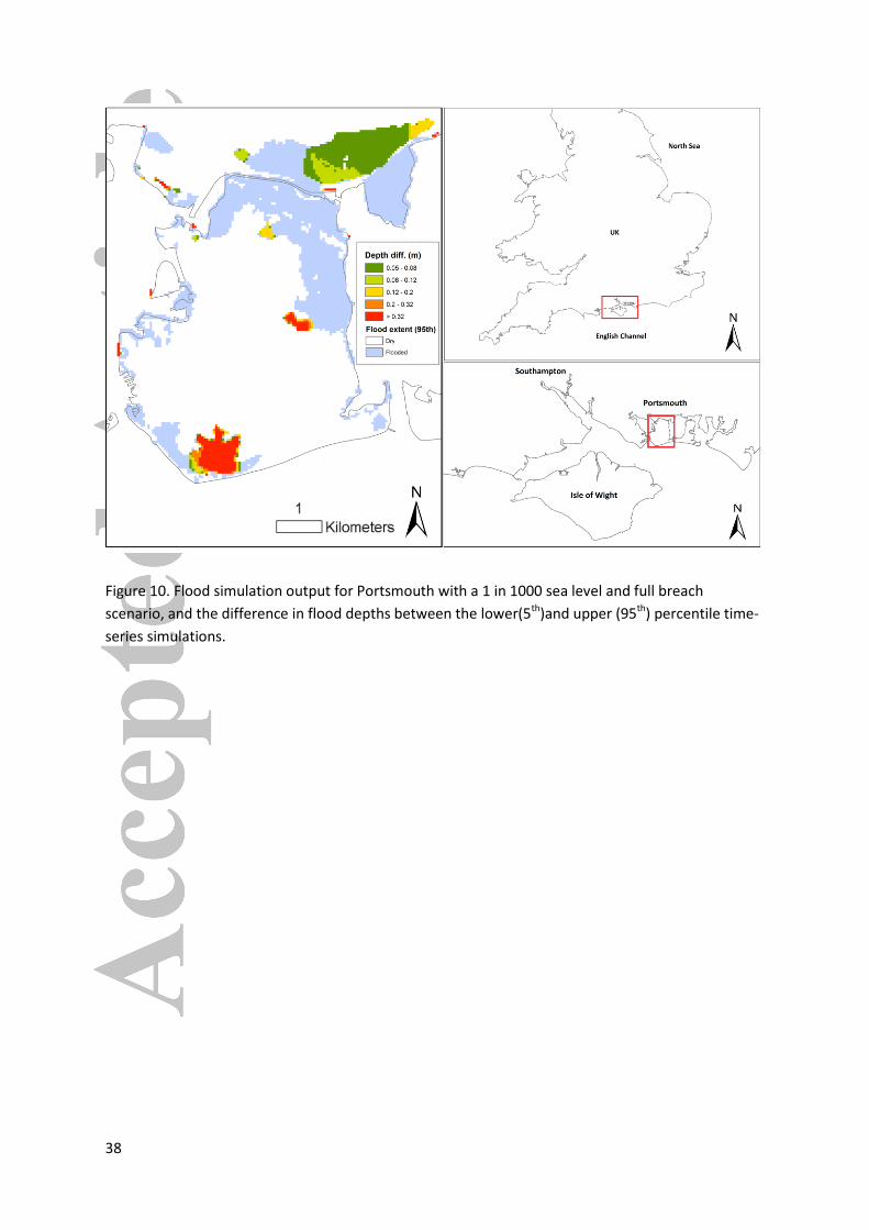
The case study assessment at Portsmouth provided a detailed insight into the consequences time-

series variability during storm-tide events might have upon flood risk predictions. Fig. 10

demonstrates the difference in the predicted inundation depth and extent when using the defined

upper and lower time-series bounds, given a worst case (full breach) scenario during a 1 in 1000 year

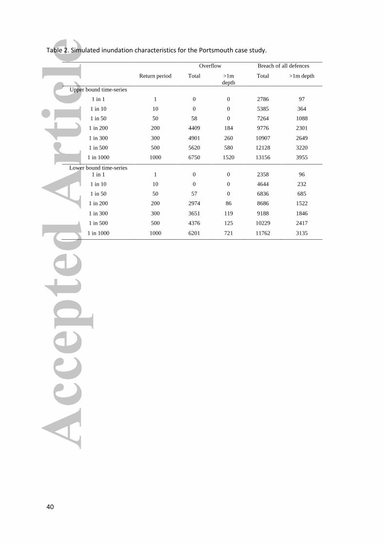
event. Table 2 provides the results from each simulation. As expected, the variability in the time-

series of a given event had a clear effect upon the expected inundation of the region due to the

duration and magnitude by which defences were exceeded. For example, where defences were held,

the implementation of the upper (95th percentile) time-series to the 1 in 1000 year event water level

resulted in a 8% increase in the expected number of properties inundated and a 53% increase in

17

those experiencing depths greater than 1 m relative to prediction made using the lower (5th

percentile) time-series.

These findings indicate that storm-tide time-series temporal variability is likely to be a significant

source of uncertainty to flood risk assessments, particularly within quantification of consequences

for extreme sea level and defence exceeding events; due to both the size of the uncertainty in the

volume of water entering the domain and the sensitivity of commonly used inundation models to

this input. Therefore, this should be accounted for in such scenarios using the methods described in

this research.

5. Conclusions

This research has demonstrated that there is considerable variability in the hours leading up to and

proceeding the maximum water levels experienced during extreme storm-tide events, which can

influence flood risk assessment. This variability has been quantified relative to a given storm-tide

peak, for each gauge, based upon the analysis of extreme (>1%) water levels since 1993. The findings

demonstrated that the magnitude of the event-mean time-series variability across the gauges

assessed ranged from 1.9% to 11.3%, with a UK average of 4.6%. Given a 1in 300 year event, the

comparison between the upper and lower bounds of storm-tide variability at each site resulted in an

event mean difference of 0.95 m when considering all UK gauges. Although the magnitude of the

variability was usually greatest during the low water; all sites contained a difference of at least 0.4 m

when considering the time-series variability within 3 hours of high water. The greatest variability was

found to occur at sites experiencing relatively low tidal ranges and large non-tidal residuals, such as

Felixstowe and Harwich in the southern North Sea.

Assuming coastal defences built to a 1 in 200 year capacity, the difference in overflow volume during

a 1 in 200, 500 and 1000 year event, due to the time-series variability at each site, was examined.

18

The results revealed that this variability resulted in a UK average difference of 73%, 69%, and 47% in

the event-mean estimated overflow volumes for the 1 in 200, 500 and 1000 year events,

respectively. A detailed case study at Portsmouth further demonstrated the importance of

quantifying the variability in storm-tide time-series for flood risk assessments, considering a range of

storm-tide magnitudes. Given a current 1 in 200 year event, the difference between the upper and

lower bounds of the storm tide variability resulted in an increase of more than 30% in the number of

buildings expected to be inundated in the region. It is therefore relevant that other case studies

should be explored, whilst it is also recommended that future inundation modelling (whether

deterministic or probabilistic) adequately represents this source of uncertainty when defining

inundation exposure and consequences.

Future research could extend the analysis to consider other coastal processes of relevance to flood

risk that might be impacted by time-series variability, such as wave-overtopping, sediment

transportation, or defence failure. For instance, it would be expected that the duration of high water

would influence the volume of wave-overtopping a section of defence might experience, while also

impacting the likelihood of defence failure due to changes in the wave loading. Similarly the time-

series uncertainty may have significant impacts upon the predicted erosion of soft coastal defences

or offshore sand banks due to the influence of water depth and wave forcing on the geomorphology

of such features. For these reasons, investigation of the effects to coastal flood risk estimates due to

uncertainty with a storm-tide time-series when applied to a multi-model system (such as the

defence over-topping-defence breaching model of Wood and Bateman, 2005) would be particularly

valuable to coastal managers.

Acknowledgements

The research presented in this paper was funded by the KULTURisk FP7-ENV-2010 project, while

M.P. Wadey and I.D. Haigh time was funded by the NERC Flood Memory EP/K013513/1 project. The

19

authors are grateful to the National Tidal and Sea Level Facility (hosted by the National

Oceanographic Centre) and the British Oceanographic Data Centre for the provision of the UK tide

gauge data used in this research. The data for this paper can be obtained from the British

Oceanographic Data Centre at: https://www.bodc.ac.uk/data/online_delivery/ntslf/processed/.

References

Ackers, P., White, W.R., Perkins, J. A., Harrison, A.J.M. (1978). Weirs and flumes for flow

measurement. Wiley, Chichester.

Barmania, S. (2014). Typhoon Haiyan recovery: progress and challenges. The Lancet, 383, 9924,

1197-1199, doi: 10.1016/S0140-6736(14)60590-0.

Bates, P.D., Horritt, M.S., Fewtrell, T.J. (2010). A simple inertial formulation of the shallow water

equations for efficient two-dimensional flood inundation modelling. Journal of Hydrology, 387, 33-

45, doi:10.1016/j.jhydrol.2010.03.027.

Bates, P. D., Dawson, R. J., Hall, J. W., Horritt, M. S., Nicholls, R. J., Wicks, J. & Mohamed Ahmed Ali

Mohamed, H. (2005). Simplified two-dimensional numerical modelling of coastal flooding and

example applications. Coastal Engineering, 52, 793-810, doi: 10.1016/j.coastaleng.2005.06.001.

Batstone, C., Lawless, M., Tawn, J., Horsburgh, K., Blackman, D., McMillan, A., Worth, D., Laeger, S. &

Hunt, T. (2013). A UK best-practice approach for extreme sea-level analysis along complex

topographic coastlines. Ocean Engineering, 71, 28-39, doi: 10.1016/j.oceaneng.2013.02.003.

Baxter, P. J. (2005). The east coast Big Flood, 31 January–1 February 1953: a summary of the human

disaster. Philosophical Transactions of the Royal Society A: Mathematical, Physical and Engineering

Sciences, 363, 1293-1312, doi: 10.1098/rsta.2005.1569.

20

Bocquet, F., Flowerdew, J., Hawkes, P., Pullen, T., and Tozer, N. (2009). Probabilistic coastal flood

forecasting: forecast demonstration and evaluation. Environment Agency Report, SC050089.

Available Online: http://cdn.environment-agency.gov.uk/scho0109bpfp-e-e.pdf.

Brown, J., Bolanos, R., Wolf, J. (2011). Impact assessment of advanced coupling features in a tide-

surge-wave model, POLCOMS-WAM, in a shallow water application. Journal of Marine Systems, 87,

1, 13-24, doi: 10.1016/j.jmarsys.2011.02.006.

Brown, J. D., Damery, S. L. (2002). Managing flood risk in the UK: towards an integration of social and

technical perspectives. Transactions of the Institute of British Geographers, 27, 4, 412-426, doi:

10.1111/1475-5661.00063.

Brown, J. D., Spencer, T. & Moeller, I. (2007). Modeling storm surge flooding of an urban area with

particular reference to modeling uncertainties: A case study of Canvey Island, United Kingdom.

Water Resour. Res., 43, W06402, doi: doi: 10.1029/2005WR004597.

Committee on Climate Change (2013) Managing the land in a changing climate – Adaptation sub-

committee progress report 2013. Available online: http://www.theccc.org.uk/publication/managing-

the-land-in-a-changing-climate/

Davis, J., Paramygin, V., Forrest, D., and Sheng, Y. (2010). Toward the probabilistic simulation of

storm surge and inundation in a limited resource environment. Monthly Weather Review, 138, 2953-

2974, doi: 10.1175/2010MWR3136.1.

Dawson, R.J., Hall, J., W, Bates, P., Nicholls, R., J. (2005a). Quantified analysis of the probability of

flooding in the Thames Estuary under imaginable worst-case sea level rise scenarios. Water

Resources Development, 21, 577-591, doi: 10.1080/07900620500258380.

21

Dawson, R., Hall, J., Sayers, P. & Bates, P. (2003). Flood risk assessment for shoreline management

planning. Proceedings of the International Conference on Coastal Management, Edited by: McInnes,

R. G., 83-97. London: Thomas Telford. ISBN: 0 7277 3255 2.

Dawson, R.J., Dickson, M.E., Nicholls, R.J., Hall, J.W., Walkden, M.J.A., Stansby, P.K, Mokrech, M.,

Richards, J., Zhou, J., Milligan, J., Jordan, A., Pearson, S., Rees, J., Bates, P.A., Koukoulas, S.,

Watkinson, A.R. (2009). Integrated analysis of coastal flooding and cliff erosion under scenarios of

long term change. Climatic Change, 95, 249-288, doi: 10.1007/s10584-008-9532-8.

Fewtrell, T. J., Bates, P. D., Horritt, M. Hunter, N. M. (2008). Evaluating the effect of scale in flood

inundation modelling in urban environments. Hydrological Processes, 22, 5107-5118, doi:

10.1002/hyp.7148.

Flather, R. (1994). A storm surge prediction model for the Northern Bay of Bengal with application to

the cyclone disaster in April 1991. Journal of Physical Oceanography, 24, 1, 172-190, doi:

10.1175/1520-0485(1994)024<0172:ASSPMF>2.0.CO;2.

Flowerdew, J., Horsburgh, K., Mylne, K. (2009). Ensemble forecasting of storm surges, Marine

Geodesy, 32, 2, 91-99, doi: 10.1080/01490410902869151.

Gallien, T. W., Schubert, J. E. & Sanders, B. F. (2011). Predicting tidal flooding of urbanized

embayments: A modeling framework and data requirements. Coastal Engineering, 58, 567-577, doi:

10.1016/j.coastaleng.2011.01.011

Gerritsen, H. (2005). What happened in 1953? The big flood in the Netherlands in retrospect.

Philosophical Transactions of the Royal Society, A, 363, 1271-1291, doi: 10.1098/rsta.2005.1568.

Gönnert, G., S.K, D., Murty, T. & Siefert, W. (2001). Global storm surges: Theory observation and

application, issue 63, Heide i. Holstein : Boyens.

22

Haigh, I.D., MacPherson, L.R., Mason, M.S., Wijeratne, E.M.S., Pattiaratchi, C.B., George, S., (2014a).

Estimating present day extreme water level exceedance probabilities around the coastline of

Australia: tropical cyclone induced storm surges. Climate Dynamics, 42, 1-2, 139-157, doi:

10.1007/s00382-012-1653-0.

Haigh, I.D., Nicholls, R., Wells, N. (2010). A comparison of the main methods for estimating

probabilities of extreme still water levels. Coastal Engineering, 57, 838-849.

doi:10.1016/j.coastaleng.2010.04.002.

Haigh, I., Nicholls, R., and Wells, N. (2011). Rising sea levels in the English Channel 1900 to 2100.

Proceedings of the ICE Maritime Engineering, 164, 2, 81-92, doi: 10.1680/maen.2011.164.2.81.

Haigh, I.D., Wijeratne, E.M.S., MacPherson, L.R., Pattiaratchi, C.B., Mason, M.S., Crompton, R.P.,

George, S., (2014b). Estimating present day extreme total water level exceedance probabilities

around the coastline of Australia: tides, extra-tropical storm surges and mean sea level. Climate

Dynamics, 42, 1-2, 121-138, doi: 10.1007/s00382-012-1652-1.

Hall, J., Solomatine, D. (2008). A framework for uncertainty analysis in flood risk management

decisions. International Journal of River Basin Management, 6, 2, 85 – 98, doi:

10.1080/15715124.2008.9635339.

Horsburgh, K., Williams, J. A., Flowerdew, J., Mylne, K. (2008). Aspects of operational forecast model

skill during an extreme storm surge event. Journal of Flood Risk Management, 1, (4), 213-221, doi:

10.1111/j.1753-318X.2008.00020.x.

Horsburgh, K., Wilson, C. (2007). Tide-surge interaction and its role in the distribution of surge

residuals in the North Sea. Journal of Geophysical Research, 112, C08003, doi:

10.1029/2006JC004033.

23

Houghton, J. (2005). Global Warming. Reports on progress in physics, 68, 1343-1403, doi:

10.1088/0034-4885/68/6/R02.

Howard, T., Lowe, J., Horsburgh, K. (2010). Interpreting century-scale changes in southern North Sea

storm surge climate derived from coupled model simulations. Journal of Climate, 23, 23, 6234-6247,

doi: 10.1175/2010JCLI3520.1.

Hunt, J. (2005). Inland and coastal flooding: developments in prediction and prevention.

Philosophical Transactions of the Royal Society A, 363, 1475-1491, doi: 10.1098/rsta.2005.1580.

Kantha, L., Clayson, C. (2000). Numerical models of oceans and oceanic processes. Academic Press:

San Diego, ISBN: 978-0-12-434068-8.

Kim, S., Yasuda, T., Mase, H. (2010). Wave set-up in the store surge along open coasts during

Typhoon Anita. Coastal Engineering, 57, 631-642, doi: 10.1016/j.coastaleng.2010.02.004.

Lewis, M., Horsburgh, K., Bates, P., Smith, R. (2011). Quantifying the Uncertainty in Future Coastal

Flood Risk Estimates for the U.K. Journal of Coastal Research, 27, 870 – 881, doi:

10.2112/JCOASTRES-D-10-00147.1.

Lewis, M., Schumann, G., Bates, P., Horsburgh, K. (2013). Understanding the variability of an extreme

storm-tide along a coastline. Estuarine, Coastal and Shelf Science, 123, 19-25, doi:

10.1016/j.ecss.2013.02.009.

Lowe, J.A., Howard, T., P, Pardaens, A., Tinker, J., Holt, J., Wakelin, S., Milne, G., Leake, J., Wolf, J.,

Horsburgh, K., Reeder, T., Jenkins, G., Ridley, J., Dye, S., Bradley, S. (2009). UK Climate Projections

science report: Marine and coastal projections, Met Office Hadley Centre, Exeter, UK. Available

online:

http://academia.edu/1892600/UK_Climate_Projections_science_report_Marine_and_coastal_proje

ctions.

24

Madsen, H., and Canizares, R. (1999). Comparison of extended and ensemble Kalman Filters for data

assimilation in coastal area modelling. International Journal for Numerical Methods in Fluids, 31,

961-981, doi: 10.1002/(SICI)1097-0363(19991130)31:6<961::AID-FLD907>3.3.CO;2-S.

Maybeck, P. (1979). Stochastic models, estimation and control, Volume 1. Academic Press: New

York. ISBN: 0-12-480701-1.

McCabe, M., Stansby, P., Apsley, D. (2013). Random wave runup and overtopping a steep wall:

Shallow-water and Boussinesq modelling with generalised breaking and wall impact algorithms

validated against laboratory and field measurements. Coastal Engineering, 74, 33-49, doi:

10.1016/j.coastaleng.2012.11.010.

Meehl, G.A., Stocker, T., F , Collins, W., D, Friedlingstein, P., Gaye, A., T, Gregory, J., M, Kitoh, A.,

Knutti, R., Murphy, J., M, Noda, A., Raper, S., C, B, Watterson, I., G, Weaver, A., J, Zhao, Z., C. (2007).

Global Climate Projections. In Climate Change 2007: The Physical Science Basis. Contribution of

Working Group I to the Fourth Assessment Report of the Intergovernmental Panel on Climate

Change [Solomon, S., D. Qin, M.M., Z. Chen, M. Marquis, K.B. Averyt, M. Tignor and H.L. Miller

(eds.)]. Cambridge, United Kingdom and New York, NY, USA. Available online:

http://www.ipcc.ch/publications_and_data/publications_ipcc_fourth_assessment_report_wg1_repo

rt_the_physical_science_basis.htm.

McMillan, A., Batstone, C., Worth, D., Tawn, J., Horsburgh, K., Lawless, M. (2011). Coastal flood

conditions for UK mainland and islands. Environment Agency project SC060064/TR2: Design sea

levels, pp142.

McRobie, A., Spencer, T. & Gerritsen, H. (2005). The Big Flood: North Sea storm surge. Philosophical

Transactions of the Royal Society A: Mathematical, Physical and Engineering Sciences, 363, 1263-

1270, doi: 10.1098/rsta.2005.1567.

25

Mokrech, M., Nicholls, R, J., Dawson, R, J. (2012). Scenarios of future built environment for coastal

risk assessment of climate change using a GIS-based multicriteria analysis. Environment and Planning

B: Planning and Design, 39, 1, 120-136, doi: 10.1068/b36077.

Neal, J. (2007). Flood forecasting and adaptive sampling with spatially distributed dynamic depth

sensors. PhD Thesis, University of Southampton, UK.

Nicholls, R., J. (1995). Coastal Megacities and Climate Change. GeoJournal, 37, 369 – 379, doi:

10.1007/BF00814018.

Pappenberger, F. & Beven, K. J. (2006). Ignorance is bliss: Or seven reasons not to use uncertainty

analysis. Water Resour. Res., 42, W05302, doi: 10.1029/2005WR004820.

Pawlowicz, R., Beardsley, B., Lentz, S. (2002). Classical tidal harmonic analysis with errors in matlab

using t-tide. Computers and Geosciences, 28, 929-937, doi: 10.1016/S0098-3004(02)00013-4.

Pugh, D.J. (1987). Tides, Surges and Mean Sea-level. A Handbook for Engineers and Scientists. Wiley,

Chichester 472pp. ISBN: 0 471 91505.

Pullen, T., Allsop, N.W.H., Bruce, T., Kortenhaus, A., Schuttrumpf, H., van der Meer, J. (2007).

Eurotop, wave overtopping of sea defences and related structures – assessment manual. Available

online: http://www.overtopping-manual.com/manual.html.

Pullen, T., Allsop, W., Bruce, T. & Pearson, J. (2009). Field and laboratory measurements of mean

overtopping discharges and spatial distributions at vertical seawalls. Coastal Engineering, 56, 121-

140, doi: 10.1016/j.coastaleng.2008.03.011.

Purvis, M., Bates, P., Hayes, C. (2008). A probabilistic methodology to estimate future coastal flood

risk due to sea level rise. Coastal Engineering, 1062-1073, doi: 10.1016/j.coastaleng.2008.04.008.

26

Quinn N., Bates, P. D., Siddall, M, (2013). The contribution to future flood risk in the Severn Estuary

from extreme sea level rise due to ice sheet mass loss. Journal of Geophysical Research: Oceans,

118, 5887-5898, doi:10.1002/jgrc.20412.

RIBA and ICE. (2009). Facing up to rising sea-levels: retreat? Defence? Attack? The future of our

coastal and estuarine cities. Royal Institute for British Architects, London, UK and Institute of Civil

Engineers,

http://www.buildingfutures.org.uk/assets/downloads/Facing_Up_To_Rising_Sea_Levels.pdf.

Roelvink, D., Reniers, A., van Dongeren, A., van Thiel de Vries, J., McCall, R., Lescinski, J. (2009).

Modelling storm impacts on beaches, dunes and barrier islands. Coastal Engineering, 56, 1133-1152,

doi: 10.1016/j.castaleng.2009.08.006.

Risk Management Solutions (2005). Hurricane Katrina: Profile of a super cat, lessons and implications

for catastrophic risk management, RMS, USA. Available inline:

https://support.rms.com/publications/KatrinaReport_LessonsandImplications.pdf.

Sekovski, I., Newton, A., Dennison, W. C. (2012). Megacities in the coastal zone: Using a driver-

pressure-state-impact-response framework to address complex environmental problems. Estuarine,

Coastal and Shelf Science, 96, 48.59, doi: 10.1016/j.ecss.2011.07.011.

Slingo, J., Belcher, S., Scaife, A., McCarthy, M., Saulter, A., McBeath, K., Jenkins, A., Huntingford, C.,

Marsh, T., Hannaford, J., Parry, S. (2014). The recent storms and floods in the UK. Available online:

http://www.metoffice.gov.uk/media/pdf/1/2/Recent_Storms_Briefing_Final_SLR_20140211.pdf.

Small, C., Nicholls, R., J. (2003). A Global Analysis of Human Settlement in Coastal Zones. Journal of

Coastal Research, 19, 3, 584 – 599. Available online:

ftp://ftp.ldeo.columbia.edu/pub/small/PUBS/SmallNichollsJCR2003.pdf.

27

Smith, R., Bates, P., Hayes, C. (2012). Evaluation of a coastal flood inundation model using hard and

soft data. Environmental Modelling and Software, 35-46, doi: 10.1016/j.envsoft.2011.11.008

Spencer, T., and French, J. (1993). Coastal flooding: transient and permanent. Geography, 78, 2, 179-

182. Available online: http://www.jstor.org/stable/40572502.

Stansby, P., Chini, N., Apsley, D., Borthwick, A., Bricheno, L., Horrillo-Caraballo, J., McCabe, M.,

Reeve, D., Rogers, B.D., Saulter, A., Scott, A., Wilson, C., Wolf, J., Yan, K. (2012). An integrated model

system for coastal flood prediction with a case history for Walcott, UK, on 9 November 2007. Journal

of Flood Risk Management, 6 (3), 229-252, doi: 10.1111/jfr3.12001.

Tawn, J. A. (1992). Estimating probabilities of extreme sea levels. Applied statistics, 41, 77-93, doi:

10.2307/2347619.

Tibbetts, J. (2002). Coastal cities: Living on the edge. Environmental Health Perspectives, 110, 11,

A674 – A681, doi: 10.1289/ehp.110-a674.

Turner, R., K, Subak, S., Adger, W., N. (1996). Pressures, Trends, and Impacts in Coastal Zones:

Interactions between Socioeconomic and Natural Systems. Environmental Management, 20, 159 –

173, doi: 10.1007/BF01204001.

Wadey, M. P., Nicholls, R. J. & Haigh, I. (2013a). Understanding a coastal flood event: the 10th March

2008 storm surge event in the Solent, UK. Natural Hazards, 67, 2, 1-26, doi: 10.1007/s11069-013-

0610-5.

Wadey. M., Nicholls, R., Hutton, C. (2012). Coastal flooding in the Solent: An integrated analysis of

defences and inundation. Water, 4, 430-459, doi: 10.3390/w4020430.

Wolf, J. (2009). Coastal flooding: impacts of coupled wave-surge-tide models. Natural Hazards, 49, 2,

241-260, doi: 10.1007/s11069-008-9316-5.

28

Zong, Y., Tooley, M. (2003). A historical record of coastal floods in Britain: frequencies and

associated storm tracks. Natural Hazards, 29, 13-36, doi: 10.1023/A:1022942801531.

29

Figure 1. Time-series of total water level, tidal and non-tidal residual at Liverpool for 8 storm-tide

events whose maximum water level is comparable.

30

Figure 2. Tide gauge sites used in the analysis.

31

Figure 3. Ensemble statistics used to quantify event time-series uncertainty.

32

Figure 4. Tide, residual and water levels associated with the top 1% of storm-tide events at

Felixstowe. Absolute tide, residual, and water level elevations are given in a, c, and e, respectively.

Tidal elevation relative to high tide is given in b, while residual elevations and water level elevations

relative to peak water are given in d and f, respectively.

33

Figure 5. Standard deviation in water levels (% of high water) every hour relative to time of high

water. Sites are ordered from STM (top) moving clockwise around the UK ending at DEV.

34

Figure 6. Event-mean standard deviation (variability) in water level time-series.

35

Figure 7. Event-mean difference in water levels at each site when contrasting the upper (95th) and

lower (5th) time-series bounds assigned to current 1 in 300 year storm-tides.

36

Figure 8. Correlation between event-mean time-series variability at each site with: tidal range (left)

and the non-tidal residual magnitude normalised relative to the tidal range (right).

37

Figure 9. The difference in estimated overflow volumes per unit area of defence when contrasting

the upper (95th) and lower (5th) time-series bounds assigned to a 1 in 300 year storm-tide at each

site.

38

Figure 10. Flood simulation output for Portsmouth with a 1 in 1000 sea level and full breach

scenario, and the difference in flood depths between the lower(5th)and upper (95th) percentile time-

series simulations.

39

Tables

Table 1. Tide gauge information

Station Name Site ID Location (Decimal Degrees) Data length (years) Lat. Long.

Aberdeen ABE 57.14 -2.08 19 Avonmouth AVO 51.52 -2.72 19 Bangor BAN 54.67 -5.67 18 Barmouth BAR 52.72 -4.05 19 Bournemouth BOU 50.72 -1.88 16 Cromer CRO 52.94 1.3 19 Devonport DEV 50.37 -4.2 19 Dover DOV 51.12 1.32 19 Felixstowe FEL 51.96 1.35 18 Fishguard FIS 52.02 -4.98 19 Harwich HAR 51.96 1.35 8 Heysham HEY 54.04 -2.93 19 Hinkley Point HIN 51.22 -3.13 19 Holyhead HOL 53.32 -4.63 17 Ilfracombe ILF 51.22 -4.11 19 Immingham IMM 53.63 -0.18 19 Jersey JER 49.19 -2.12 19 Kinlochbervie KIN 58.46 -5.05 19 Leith LEI 55.99 -3.18 19 Lerwick LER 60.15 -1.12 14 Liverpool LIV 53.45 -3.02 19 Llandudno LLA 53.33 -3.83 18 Lowestoft LOW 52.48 1.77 19 Milford Haven MHA 51.71 -5.05 19 Millport MIL 55.76 -4.91 19 Moray Firth MOR 57.6 -4 10 Mumbles MUM 51.57 -3.98 19 Newhaven NHA 50.78 0.05 19 Newlyn NEW 50.11 -5.55 19 Newport NPO 51.55 -2.99 19 North Shields NSH 55.01 -1.44 19 Port Ellen ISL 55.64 -6.2 18 Port Erin IOM 54.09 -4.77 19 Portpatrick POR 54.85 -5.12 19 Portrush PRU 55.21 -6.67 17 Portsmouth PTM 50.81 -1.11 17 St. Mary's STM 49.93 -6.32 18 Sheerness SHE 51.45 0.74 19 Stornoway STO 58.2 -6.39 19 Tobermory TOB 56.63 -6.07 15 Ullapool ULL 57.89 -5.16 15 Weymouth WEY 50.61 -2.45 19 Whitby WHI 54.51 -0.62 19 Wick WIC 58.45 -3.08 15 Workington WOR 54.66 -3.57 16

40

Table 2. Simulated inundation characteristics for the Portsmouth case study.

Overflow Breach of all defences

Return period Total >1m

depth

Total >1m depth

Upper bound time-series

1 in 1 1 0 0 2786 97

1 in 10 10 0 0 5385 364

1 in 50 50 58 0 7264 1088

1 in 200 200 4409 184 9776 2301

1 in 300 300 4901 260 10907 2649

1 in 500 500 5620 580 12128 3220

1 in 1000 1000 6750 1520 13156 3955

Lower bound time-series

1 in 1 1 0 0 2358 96

1 in 10 10 0 0 4644 232

1 in 50 50 57 0 6836 685

1 in 200 200 2974 86 8686 1522

1 in 300 300 3651 119 9188 1846

1 in 500 500 4376 125 10229 2417

1 in 1000 1000 6201 721 11762 3135