A Feasibility Study of Dynamical Assimilation of Tide Gauge ...

Old Dominion University Old Dominion University

ODU Digital Commons ODU Digital Commons

OES Theses and Dissertations Ocean & Earth Sciences

Spring 1995

A Feasibility Study of Dynamical Assimilation of Tide Gauge Data A Feasibility Study of Dynamical Assimilation of Tide Gauge Data

in the Chesapeake Bay in the Chesapeake Bay

Yvette H. Spitz Old Dominion University

Follow this and additional works at: https://digitalcommons.odu.edu/oeas_etds

Part of the Atmospheric Sciences Commons, and the Oceanography Commons

Recommended Citation Recommended Citation Spitz, Yvette H.. "A Feasibility Study of Dynamical Assimilation of Tide Gauge Data in the Chesapeake Bay" (1995). Doctor of Philosophy (PhD), Dissertation, Ocean & Earth Sciences, Old Dominion University, DOI: 10.25777/hya6-a208 https://digitalcommons.odu.edu/oeas_etds/78

This Dissertation is brought to you for free and open access by the Ocean & Earth Sciences at ODU Digital Commons. It has been accepted for inclusion in OES Theses and Dissertations by an authorized administrator of ODU Digital Commons. For more information, please contact [email protected].

https://digitalcommons.odu.edu/

https://digitalcommons.odu.edu/oeas_etds

https://digitalcommons.odu.edu/oeas

https://digitalcommons.odu.edu/oeas_etds?utm_source=digitalcommons.odu.edu%2Foeas_etds%2F78&utm_medium=PDF&utm_campaign=PDFCoverPages

http://network.bepress.com/hgg/discipline/187?utm_source=digitalcommons.odu.edu%2Foeas_etds%2F78&utm_medium=PDF&utm_campaign=PDFCoverPages

http://network.bepress.com/hgg/discipline/191?utm_source=digitalcommons.odu.edu%2Foeas_etds%2F78&utm_medium=PDF&utm_campaign=PDFCoverPages

https://digitalcommons.odu.edu/oeas_etds/78?utm_source=digitalcommons.odu.edu%2Foeas_etds%2F78&utm_medium=PDF&utm_campaign=PDFCoverPages

mailto:[email protected]

A FEA SIBILITY STUDY OF DYNAMICAL ASSIMILATION OF

T ID E GAUGE DATA IN TH E CHESA PEAK E BAY

by

Y vette H. Spitz

M.Sc., April 1990, Florida S tate University, Tallahassee, Florida, U.S.A. Licence in Physics, October 1983, Liege University, Liege, Belgium

A Dissertation subm itted to the Faculty of Old Dominion University in P artia l Fulfillment of the

Requirem ents for the Degree of

Doctor o f Philosophy

Oceanography

Old Dominion University May, 1995

Approved by:

John M . Klinck (Director)

Larry P. Atkinson

G abriel T . Csanady

Linda M. Lawson

Ionel M. Navon

Reproduced with permission of the copyright owner. Further reproduction prohibited without permission.

Abstract

A FEA SIBILITY STUDY OF DYNAMICAL ASSIMILATION OF T ID E GAUGE DATA IN TH E CHESAPEAKE BAY

Yvette H uberte Spitz

Old Dominion University, 1995 Director: Dr. J . M. Klinck

The feasibility of dynam ical assimilation of surface elevation from tide gauges

is investigated to estim ate the bottom drag coefficient and surface stress as a first

step in improving modeled tidal and wind-driven circulation in the Chesapeake Bay.

A two-dimensional shallow water model and an adjoint variational m ethod with a

lim ited m em ory quasi-Newton optim ization algorithm are used to achieve this goal.

Assimilation of tide gauge observations from ten perm anent stations in the Bay

and use of a two-dimensional model adequately estim ate the bottom drag coefficient,

wind stress and surface elevation at the Bay m outh. Subsequent use of these esti

m ates in the circulation model considerably improves the modeled surface elevation

in the entire Bay. Assimilation of predicted tidal elevations yields a drag coefficient,

defined in the hydraulic way, varying between 2.5 x 10-4 and 3.1 x 10-3 . The bottom

drag coefficient displays a periodicity corresponding to the spring-neap tide cycle.

From assim ilation of actual tide gauge observations, it is found th a t the fortnightly

m odulation is altered during frontal passage. Furtherm ore, the response of the sea

surface to the wind forcing is found to be more im portan t in the lower Bay than in

the upper Bay, where the barom etric pressure effect could be more im portant.

In addition, identical twin experiments with model generated da ta show th a t a


penalty term has to be added to the simple cost function defined as the distance

between m odeled and observed surface elevation in order to assure sm oothness of

the surface elevation field a t the Bay m outh. Classical scaling of th e param eters

to bring them to the same order of m agnitude was not effective in accelerating

the convergence during the assimilation procedure and yielded larger errors in the

estim ated param eters.


Acknowledgments

I wish to express my g ratitude to Dr. John Klinck, my dissertation advisor,

for his support, guidance and encouragement in pursuing the independent research

which comprises this work. I thank the members of m y com m ittee, Drs. Larry

Atkinson, Gabriel Csanady, Linda Lawson and Ionel Navon, for their interest in

my work as well as their help and suggestions. My special thanks go to Dr. Linda

Lawson for her great help, expertise in da ta assimilation, kindness, constant encour

agement and for the understanding th a t she has shown these past three years. I

am also grateful to Dr. Ionel Navon and Dr. X. Zou of F lorida S ta te University for

sharing their expertise in d a ta assim ilation as well as in adjoint model coding and

pointing out the im portant references related to the variational m ethod. I also thank

Dr. Larry Atkinson for his support and for providing a wonderful working environ

m ent a t CCPO . I thank Dr. Eileen Hofmann, CCPO, for giving m e the opportunity

to apply the variational da ta assim ilation technique to a m arine ecosystem model.

This work w ith Drs. Linda Lawson, ETSU, and Eileen Hofmann afforded me the

opportunity to explore the field of biological-physical modeling. Thanks are due to

Dr. Arnoldo Valle-Levinson, CC PO , for the numerous productive discussions we

had regarding tidal modeling and the Chesapeake Bay. I thank the Commonwealth

of V irginia and the Center for Coastal Physical Oceanography for supporting this

research.

I thank the M anagement U nit of the M athem atical Models of the North Sea and

Scheldt Estuary, especially Dr. Georges Pichot and Jose Ozer, for allowing me to

use their model. Dr. Steve Gill and Captain Carl Fisher, of NOAA, provided the

d a ta and tidal analysis used in th is work. Dr. John Hamrick, VIMS, provided the

model grid used in the sim ulations. Their assistance is greatly appreciated.

ii


Finally, I am very grateful to my m other and sister who have always been sup

portive during my studies far from home. All the faculty members, students and

staff members a t CCPO and from the D epartm ent of Oceanography are thanked for

their friendship and encouragement over the last four years.

111


Contents

1 Introduction 1

2 Background 6

2.1 Physical characteristics of the Chesapeake Bay and its tribu taries . . 7

2.2 Observations in the Chesapeake B a y .......................................................... 9

2.3 Circulation in the Chesapeake B a y .................................................................. 13

2.3.1 Tidal circulation ....................................................................................... 13

2.3.2 W ind-driven c i r c u la t io n ......................................................................... 20

3 Method 24

3.1 O verview ..................................................................................................................... 24

3.2 Circulation m o d e l .................................................................................................... 29

3.3 Cost f u n c t i o n ...........................................................................................................32

3.4 Adjoint m o d e l ...........................................................................................................35

3.4.1 Tangent linear model t e c h n iq u e ............................................................36

3.4.2 Lagrange m ultiplier m e t h o d ..................................................................38

3.4.3 Verification of adjoint code and gradient of the cost function . 39

3.5 O ptim ization te c h n iq u e s ...................................................................................... 40

3.6 D ata assim ilation in Chesapeake B a y .............................................................. 43

4 Results 52

4.1 Identical twin e x p e rim e n ts ....................................................................................53

4.1.1 Model derived observations ...................................................................53

4.1.2 R ecovery ....................................................................................................... 55

4.2 T idal C ir c u la t io n ..................................................................................................... 74

4.2.1 Observations and s im u la tio n ...................................................................74

4.2.2 R ecovery ....................................................................................................... 83

iv


4.3 W ind-driven c irc u la t io n .......................................................................................93

4.3.1 Observations .............................................................................................. 95

4.3.2 R ecovery.........................................................................................................99

4.3.3 Further investigation of the r e c o v e r y ................................................108

5 Discussion 112

5.1 Identifiability and regularization in param eter e s t im a t io n ......................113

5.2 D ata assim ilation and twin experim en ts........................................................114

5.2.1 Definition of the cost f u n c t io n ..............................................................114

5.2.2 Scaling of the control variab les..............................................................116

5.2.3 R ate and precision of the recovery .......................................................117

5.3 D ata assim ilation and Chesapeake B a y ........................................................118

5.3.1 Estim ate of the bottom stress and drag coeffic ien t........................118

5.3.2 Atm ospheric forces in the B a y ..............................................................123

5.4 Future s tu d y ............................................................................................................. 125

6 Conclusions 129

References 131

Appendices 144

A Construction of the adjoint code 145

A .l Tangent linear model m e t h o d ......................................................................... 145

A .2 Lagrange m ultiplier te c h n iq u e ......................................................................... 148

B Optimization algorithms 151

B .l Conjugate-gradient m e t h o d ............................................................................ 152

B.2 Newton m ethod and its v a ria tio n s ..................................................... 154

B.2.1 Newton and truncated Newton m e t h o d s .........................................154

v


B.2.2 Quasi-Newton and lim ited m em ory quasi-Newton m ethods . . 155

C P e r fo rm a n c e o f t h e t id a l d a ta a s s im ila t io n 159

vi


List of Tables

1 Tide gauge stations part of the National Tide and W ater Level O b

servation Network......................................................................................................11

2 Sum m ary of the param eter values used to generate the set of obser

vations for the identical twin experim ents.........................................................54

3 Am plitude (m) and phase (deg.) for the m ajor harm onic constituents

a t ten perm anent and nine comparison tide gauge stations (Fisher,

1986).......................................................................................................................... 77

4 M inimum, m axim um and mean value of the root-m ean square error

(cm), the relative average error (%) and the correlation coefficient

for November 2 to November 19, 1983. The first ten stations are the

perm anent stations while the last nine are the comparison stations. . 85

5 Root-mean square error (cm) (first num ber), relative average error

(%) (second num ber), and correlation coefficient (th ird num ber) for

the wind-driven e x p e r im e n t ..............................................................................102

6 Root-mean square error (cm) at ten perm anent and nine com pari

son tide gauge stations for November 2 to November 10, 1983. The

first num ber corresponds to the experim ent with cp = 0.002 and the

second num ber corresponds to the recovery experim ent..........................160

7 Root-mean square error (cm) at ten perm anent and nine comparison

tide gauge stations for November 11 to November 19, 1983. The

first num ber corresponds to the experim ent with cd = 0.002 and the

second num ber corresponds to the recovery experim ent..........................161

with permission of the copyright owner. Further reproduction prohibited without permission.

8 Relative average error (%) at ten perm anent and nine comparison tide

gauge stations for November 2 to November 10, 1983. The first num

ber corresponds to the experiment with cjr> = 0.002 and the second

num ber corresponds to the recovery experim ent........................................... 162

9 Relative average error (%) at ten perm anent and nine comparison

tide gauge stations for November 11 to November 19, 1983. The

first num ber corresponds to the experiment w ith cp — 0.002 and the

second num ber corresponds to the recovery experim ent............................. 163

10 Correlation coefficient a t ten perm anent and nine comparison tide

gauge stations for November 2 to November 10, 1983. The first num

ber corresponds to the experiment with cp = 0.002 and the second

num ber corresponds to the recovery experim ent........................................... 164

11 Correlation coefficient a t ten perm anent and nine comparison tide

gauge stations for November 11 to November 19, 1983. The first

num ber corresponds to the experiment with cp = 0.002 and the sec

ond num ber corresponds to the recovery experim ent...................................165

viii


List of Figures

1 D epth contours of the Chesapeake Bay expressed in feet (Fisher,

1986).......................................................................................................................... 8

2 Overview of tide and current station deployments in the Chesapeake

Bay and its tributaries (Fisher, 1986; Browne and Fisher, 1988). . . . 12

3 Superposition of coam plitude and cophase lines of M 2 tide (Fisher,

1986). Cophase lines (solid) are expressed in degrees and coam plitude

lines (dashed) in feet.................................................................................................15

4 Superposition of coam plitude and cophase of K \ tide (Fisher, 1986).

Cophase lines (solid) are expressed in degrees and coam plitude lines

(dashed) in feet...........................................................................................................16

5 M 2 tidal current cospeed lines expressed in centim eters per second

(Fisher, 1986).......................................................................................................... 17

6 M 2 tidal current cophase lines expressed in degrees (Fisher, 1986). . . 18

7 Power spectra of sea level, a t (I) K iptopeake Beach, (II) Lewisetta,

(III) Solomons Island and (IV) Annapolis. (W ang and Elliott, 1978). 21

8 Schematic of the steps involved in the da ta assim ilation scheme. The

solid lines indicate the m ain path taken during the procedure....................30

9 Staggered grid and indexing used in the model. T he variables inside

of the dotted box have the same value of the indexes i and j ......................33

10 Verification of the gradient of the cost function using Taylor expansion. 41

11 Model domain (dotted line) and grid. The dots represent grid points. 46

ix


12 Locations of the tide gauge stations and buoys. The circles indi

cate perm anent gauges and the squares indicate the stations used

for comparison between modeled and observed elevations. The stars

represent buoys. TPLM 2 and CHLV2 designate the buoy a t Thom as

Point and Chesapeake Light Tower, respective ly ..........................................48

13 M ap of the relative average error (%) over 24 hours between m odeled

elevation using the first guess control param eters and the observations

for a northeasterly wind...........................................................................................57

14 M ap of the relative average error (%) over 24 hours between m odeled

elevation using th e first guess control param eters and the observations

for a southwesterly w ind..........................................................................................58

15 Difference between recovered and true values for the m odel param e

ters and boundary elevation a t the southern end of the Bay m outh

24 hours after the beginning of the recovery day versus the num ber

of m inim ization iterations. The da ta are available everywhere and a

northeasterly wind is considered........................................................................... 59

16 Logarithm of the cost function normalized by its initial value (a)

and logarithm of the normalized norm of the gradient of the cost

function (b) versus the num ber of iterations. The d a ta are available

everywhere and a northeasterly wind is considered.........................................61

17 Map of the relative average error (%) over 24 hours between recovered

and observed surface elevation after 15 iterations of the assim ilation

process. The d a ta are available everywhere and a northeasterly wind

is considered................................................................................................................ 62


18 Difference between recovered and true values for the model param e



of m inim ization iterations. The d a ta are available a t ten stations and

a northeasterly wind is considered....................................................................... 64

19 Logarithm of the normalized cost function (a) and normalized norm of

the gradient of the cost function (b) versus the num ber of iterations.

T he d a ta are available a t ten stations and a northeasterly wind is

considered....................................................................................................................65

20 M ap of the relative average error (%) over 24 hours between recovered


process. The da ta are available a t ten stations and a northeasterly

wind is considered.....................................................................................................66

21 Difference between recovered and tru e values for the model param e



of m inim ization iterations. The da ta are available a t ten stations and

a southwesterly wind is considered...................................................................... 68

22 Logarithm of the normalized cost function (a) and normalized norm

of the gradient of the cost function (b) versus the num ber of iterations

when a southwesterly wind is blowing and da ta are available a t ten

sta tions.........................................................................................................................69

23 M ap of the relative average error (%) over 24 hours between recovered


process. The da ta are available a t ten stations and a southwesterly

wind is considered.....................................................................................................70

xi


24 Difference between recovered and true values for the m odel param e

ters and boundary elevation a t th e southern end of the Bay m outh

24 hours after the beginning of th e recovery day versus th e num ber of

m inim ization iterations. The d a ta are available everywhere, a north

easterly wind is considered, and th e penalty term is not added to the

cost function............................................................................................................... 72

25 Recovered boundary elevation from the southern to the northern end

of the Bay m outh with a penalty term in the cost function (solid line)

and w ithout the penalty term (dotted line)......................................................73

26 Difference between recovered w ith scaling of the M anning’s roughness

and true values for the model param eters and boundary elevation at

the southern end of the Bay m outh 24 hours after the beginning of the

recovery day versus the num ber of minimization iterations. The da ta

are available at ten stations and a northeasterly wind is considered. . 75

27 Logarithm of the normalized cost function (a) and norm alized norm

of the gradient of the cost function (b) versus the num ber of iterations

when a northeasterly wind is blowing and the M anning’s roughness

is scaled........................................................................................................................76

28 Tim e series of predicted sea surface elevation (m) a t B altim ore and

CBBT for November 1 to November 20, 1983.............................................. 78

29 Tim e series of modeled (dotted line) and predicted (solid line) surface

elevation (m) at six representative perm anent tide gauge stations.

The drag coefficient was taken as cp = 0.002. Note the change of

scale for the last two stations................................................................................ 80

30 Coam plitude lines of the modeled M 2 tide expressed in fee t........................81

31 Cophase lines of the modeled M 2 tide expressed in degrees......................... 82

xii



elevation (m) a t six perm anent tide gauge stations. Note the change

of scale for the last two stations........................................................................... 86


elevation (m) a t six comparison tide gauge stations......................................87

34 Tim e series of relative average error (%) for recovered (solid line) and

m odeled (cp = 0.002) (dotted line) surface elevations a t six perm a

nent tide gauge stations 88

35 Tim e series of relative average error (%) for recovered (solid line) and

modeled (cp = 0.002) (dotted line) surface elevations a t six com par

ison tide gauge stations........................................................................................... 89

36 Coam plitude of the recovered M 2 tide expressed in feet................................ 91

37 Cophase of the recovered M 2 tide expressed in degrees..................................92

38 Tim e series of estim ated bottom drag coefficient cp for depths be

tween 2 and 50 m 94

39 Tim e series of predicted tidal (solid line) and observed (dotted line)

elevation in Baltim ore and CBBT for November 1 to November 10,

1990........................................................................................................................... 96

40 Hourly observed wind in November 1990 at two buoys, Thom as Point

and Chesapeake Light Tower, and a t the tide gauge station CBBT.

The stick diagram is plotted using the oceanographic convention. . . 98

41 Tim e series of modeled (dotted line) and observed (solid line) surface

elevation (m) a t six perm anent tide gauge stations...................................... 100

42 Tim e series of relative average error (%) between modeled and ob

served surface elevation at six perm anent tide gauges. Note the

change of scale for the last three stations........................................................ 101


43 Recovered and observed wind at Thom as Point. The recovered wind,

p lo tted a t the m iddle of the recovery day, is constant during th a t day. 104

44 Recovered and observed wind at CBBT. The recovered wind, p lo tted

a t the middle of the recovery day, is constant during th a t day. . . . . 105

45 November 1990 tim e series of recovered bottom drag coefficient c#

for depths between 2 and 50 m ............................................................................106

46 T im e series of hourly boundary surface elevation (m) from the south

ern end to the northern end of the Bay m ou th .............................................. 107

47 Tim e series of observed (dotted line) and predicted (solid line) ele

vation at Baltim ore and CBBT from Septem ber 18 to Septem ber 24,

1983............................................................................................................................ 109

48 Septem ber 1983 tim e series of recovered (dotted line) and observed

(solid line) surface elevation (m) a t th ree perm anent and three com

parison tide gauge stations....................................................................................110

49 Root-m ean square errors a t stations in the Arabian Gulf for 100 days

following the beginning of the assim ilation period. T he errors are

shown before (dotted line) and after (solid line) optim ization. (Lard-

ner et al., 1993)...................................................................................................... 122

50 Barom etric pressure (mb) from November 1 to November 10, 1990. . 126

xiv

with permission of the copyright owner. Further reproduction prohibited without permission.

1 Introduction

Chesapeake Bay, the largest estuary in the United States, is not only a m ajor water

way for commercial m arine transportation, naval operations and recreational boating

bu t also a highly productive m arine environment. For instance, larvae and postlar

vae of fishes and crab, which have been spawned in the coastal ocean, re-enter the

Bay in late sum m er and early fall. Because of its in terrelation w ith other processes

taking place in the Chesapeake Bay, e.g., water quality and biological productivity,

circulation in the Bay is probably the first process th a t needs to be understood.

The m ain components of the estuarine circulation are the tidal, gravitational and

wind-driven circulation. During the last 40 years, circulation in the Bay has mainly

been studied from observations of tem perature, salinity, sea level, and currents.

P ritchard (Officer, 1976) has extensively studied the gravitational circulation while

Wang and Elliott (1978), Wang (1979a,b) have analyzed th e response of the Bay

to the wind forcing, and recently, Paraso and Valle-Levinson (1995) have studied

the response of the lower Bay to atm ospheric forcings, i.e., wind and barom etric

pressure. An extensive analysis of th e tidal circulation from tide gauge sea level and

current m easurem ents was done by Fisher (1986). These studies helped to recognize

th a t wind and bottom stress greatly influence the circulation in the Bay. However,

wind stress and bottom friction are difficult to estim ate. For instance, the wind

speed and direction are essentially m easured at m ajor airports on the western side

of the Bay. But, conversion of the wind on land to wind over w ater is not an easy

task. For instance, Goodrich (1985) showed th a t a different correction has to be done

1


to the alongshore and cross-shore wind components m easured at airports. Bottom

friction, while hard to measure, is usually defined in the two-dimensional models as

a quadratic function of the vertically-integrated velocity. An em pirical param eter,

the bottom drag coefficient, is ad justed for a best fit between the modeled surface

elevations and observations at tid e gauge stations (Crean et al., 1988).

Recently, variational da ta assim ilation and inverse m ethods have been used to

determ ine the bottom drag coefficient. Using a two-dimensional model and assim

ilation of tide gauges data, Das an d Lardner (1992), Lardner et al. (1993) showed

th a t a depth correction and b o tto m friction coefficient can be estim ated. Using an

inverse m ethod and tidal current measurem ents, Bang (1994) estim ated the bottom

drag coefficient in the Chesapeake Bay. The study from Lardner et al. (1993) in

the Arabian Gulf is probably m ost closely related to our study. However, several

m ajor differences can be pointed out. In our study, the bottom drag coefficient is

not only estim ated but also the surface forcing, and the tide gauges located close to

the coast are used, which is far m ore challenging than the use of open water gauges.

Finally, the drag coefficient param eterization is different in both studies.

D ata assimilation techniques have been recently developed in meteorology as

well as in oceanography and are num erous (Ghil et al., 1981; Navon, 1986; Ghil

and Malanotte-Rizzoli, 1991; Navon et al., 1992b,c). Most of these methods fit in

one of the following classes: i) local polynomial interpolation m ethods (Cressman,

1959), ii) statistical (optimal) in terpolation methods (Lorenc, 1981), iii) variational

num erical analysis. The la tter technique was originated in meteorology by Sasaki

(1955, 1970) and has been developed considerably since then. It addresses the

question of sensitivity analysis (Cacuci, 1981; Hall et al., 1982; Hall and Cacuci,

1983; Cacuci and Hall, 1984; Cacuci, 1988; Zou et al., 1993b), variational adjustm ent

(Lewis and Derber, 1985; Talagrand and Courtier, 1987; Thacker and Long, 1988,

Navon et al., 1992a) and param eter estimation (Panchang and O ’Brien, 1989; Das

2


and Lardner, 1991; Sm edstad and O ’Brien, 1991; Yu and O ’Brien, 1991; Zou et al.,

1992b; Lardner, 1993; Lawson et a l, 1995a,b). This list of references represents only

a small sam ple of what has been done in d a ta assimilation.

The objective of variational da ta assimilation is to m inim ize a cost function

w ith respect to the control variables by minimizing the misfit between model equiv

alents of the da ta and observations. The goodness-of-fit of the m odel equivalents

of the d a ta to the observations is m easured by a cost function, which is minimized

by adjusting the control variables. Most of the optim ization algorithm s are based

on iterative descent large-scale unconstrained local m inim ization m ethods which re

quire the com putation of the gradient of the cost function w ith respect to the control

variables. The adjoint of the model equations is used to com pute th e gradient of the

cost function. The adjoint model equations can be derived by using different m eth

ods: the derivation of Euler-Lagrange equations (Morse and Feshbach, 1953), the

control theory (Le D im et and Talagrand, 1986), the Lagrange m ultiplier approach

(Thacker and Long, 1988). In those m ethods, the continuous adjoint equations are

first derived then discretized. However, recent studies have shown th a t the adjoint

m odel code can be derived directly from the model code, which has two m ain ad

vantages. It reduces the complexity of the construction of the adjoint model and

it avoids the inconsistency th a t can arise from the derivation of th e adjoint model

followed by its discretization due to non-com m utativity of adjoint and discretiza

tion operations. Navon et al. (1992a) and Talagrand (1991) derived the adjoint

m odel code from the tangent linear model code while Lawson et al. (1995a) used

the Lagrange m ultiplier approach to derive the adjoint code from the direct model

code. The variational adjoint assimilation algorithm includes four parts: the direct

m odel, the construction of the adjoint code of the forward model, the com putation

of the cost function and its gradient w ith respect to the control param eters, and the

large-scale unconstrained local optim ization algorithm.

3


The objective of th is study is to assim ilate tide gauge observations in order to

estim ate the im portant m odel param eters, i.e., bottom and wind stress, and get

the best representation of the circulation in the Bay. This goal was achieved by

using a two-dimensional (2-D), vertically-integrated shallow w ater equations model.

Several studies for the English Channel (Ozer and Jam art, 1988; Ja m art and Ozer,

1989; W erner and Lynch, 1987) have indeed recognized th a t the 2-D, inviscid shallow

water equations can provide an accurate solution to the problem of tida l propagation.

The assim ilation technique is the variational adjoint m ethod where the adjoint model

code is obtained from the tangen t linear version of the model code. T he minimization

algorithm used to m inim ize the cost function is the lim ited m em ory quasi-Newton

m ethod developed by G ilbert and Lemarechal (1989) which is sim ilar to the m ethod

developed by Liu and Nocedal (1989).

Specifically, the results obtained from the assim ilation study address the follow

ing questions:

• How can variational d a ta assim ilation be used to determ ine th e forcing in the

model, i.e wind stress and bo ttom friction? Can we estim ate the spatial and/or

tim e dependence of the bo ttom friction and wind stress using tide gauge data?

• Is the num ber of tide gauges adequate to predict the sea level in the bay? Are the

gauges well d istributed around the bay?

• Can variational d a ta assim ilation be used to determ ine the adequacy of a two-

dimensional model to reproduce the main features of the circulation in the Chesa

peake Bay?

Section 2 contains background information on the physics and the circulation of

4


the Chesapeake Bay. Section 3 contains details of the variational adjoint da ta as

sim ilation m ethod, the direct model and application of d a ta assim ilation to the Bay.

T he results of surface elevation assimilation in the case of identical twin experim ents,

tidal and wind-driven circulation experiments using the tide gauge observations are

given in Section 4 while they are discussed in Section 5. Conclusions of th is study

are presented in Section 6.

5


2 Background

The first question th a t might be asked is “what is an estuary?” . Historically, the

term estuary comes from the latin nam e aetus, which means tide, and applied to

the lower tidal reaches of rivers. Cameron and Pritchard (1963) extended the def

inition as follows: “ An estuary is a semi-enclosed body of water which has a free

connection with th e open ocean and within which seawater is m easurably d iluted

with fresh water derived from land drainage” . Estuaries have been classified based

on two criteria: 1) geomorphological properties (Pritchard , 1952a; Dyer, 1973) and

2) circulation and stratification patterns (Dyer, 1973). In term s of shape, an es

tuary can be of th ree types: coastal plain, deep basin, and bar-built estuary. In

term s of the water properties, an estuary can be classified as highly stratified salt

wedge type, highly stratified, partially mixed and vertically homogeneous. Com

plete descriptions of estuary types can be found in Dyer (1973) and Pickard and

Em ery (1982). In the past decades, the m ain focus of estuarine studies has been

on tidal and gravitational circulation as well as river runoff. Only recently, it has

been acknowledged th a t wind-driven circulation m ight a t tim es be more im portan t

than the gravitational circulation. In the following sections, the physical character

istics of the Chesapeake Bay, the field observations, and the tidal and wind-driven

circulation in the Bay are briefly described.

6


2.1 Physical characteristics of the Chesapeake Bay and its tributaries

Chesapeake Bay is the largest estuary in the United States w ith a length of roughly

310 km, a w idth averaging 30 km (Fig. 1) and a complex topography. The Bay

can be divided into two regions which have different dimensional and physical char

acteristics: the m ain stem and the tributaries (over 50). The m ain stem which is

very narrow at the entrance (18.5 km ) widens to about 35 km near the m outh of

the Potom ac River. I t then narrows to about 6 km near the m outh of the Severn

River. Its m ain axis is directed north-south except in the lower part where it is

in the northw est-southeast direction. The m ain stem has an average depth of 8 m

with a m axim um depth , nearly 53 m , off Kent Island. The 18 ft (5.5 m) and 36 ft

(11 m) depth contours are shown in Fig. 1. The depth contours show th a t there is

a complicated system of channels starting at the Bay m outh and branching into the

tributaries. Two m ain channels and a th ird narrow channel s ta rt a t the entrance of

the Bay. The southern channel in the entrance extends westward as Thim ble Shoal

channel and branches up the Jam es River. The m ain channel extends into the main

stem while the northern channel, very narrow and deep, extends northw ard along

the eastern shore into the Pocomoke sound. The m ajor tribu taries of the lower Bay

are the Rappahannock, York, and Jam es Rivers which account for approxim ately

20% of the freshwater input in the Bay. The Potom ac and Susquehanna Rivers are

the m ajor tribu taries of the upper Bay, w ith the Susquehanna accounting for about

50% of the to ta l freshwater input.

Based on geomorphological properties (Pritchard, 1952a), th e Chesapeake Bay

has been classified as drowned river valley or coastal plain estuary. After the glacial

period, roughly 10 thousand years ago, the Chesapeake Bay system was formed.

Before sea level rose about 100 m following the glacial period, the Susquehanna River

reached the ocean about 180 km seaward of the present shoreline and the York and

7


Figure 1: D epth contours of the Chesapeake Bay expressed in feet (Fisher, 1986).


o ther rivers were tributaries of the Susquehanna River. Based on the circulation and

stratification patterns, the lower Bay has been classified as vertically homogeneous

w ith lateral variations of salinity during normal runoff conditions (Pritchard , 1952b).

In th a t region, tidal flow is dom inant. The upper Bay and the tributaries have been

classified as slightly stratified. Due to the river discharge and the tide, a two layer

circulation is present w ith a net seaward flow of fresh w ater in the upper layer and

a net flow of saline w ater toward the head in the lower layer.

2.2 Observations in the Chesapeake Bay

Observations are required not only to understand the circulation in the Bay but also

to verify the success of the num erical models and to estim ate model param eters us

ing da ta assim ilation techniques. The most useful inform ation comes from synoptic

data . The Chesapeake Bay has now been m onitored for decades by several labo

ratories and universities and m easurem ents include sea level, current, tem perature,

salinity, water quality as well as meteorological observations. Below is a brief review

of the publically available observations.

• W ater level and current

For m ore than a century, tide and tidal currents have been observed in the Chesa

peake Bay. The first tide station was installed in Annapolis in 1844 (Haight et al.,

1930; Hicks, 1964; Fisher, 1986). Prior to 1964, more than 200 tide gauge stations

and over 100 near-surface current stations were deployed. However, they were not

usually deployed for a long tim e or a t the same tim e. From those stations, ten

tide gauge stations in the Chesapeake Bay and its tribu taries are now part of the

N ational T ide and W ater Level Observation Network (Table 1) and are perm anent

installations m aintained by the National Oceanic and Atm ospheric Adm inistration

(NOAA). In addition to those long term measurements, two extensive tide and cur-

9


rent surveys of the Chesapeake Bay were conducted from 1970 to 1974 and from

1981 to 1983 (Fig. 2) by the National Ocean Survey to update tide and tidal current

predictions and to provide tidal datum for shoreline boundary determ ination.

• Meteorological observations

For a long tim e, meteorological observations were collected only a t the m ajor air

ports, e.g., Baltim ore, W ashington DC, Norfolk International Airports and Patuxent

River Naval Air Station. It is only recently th a t meteorological observations became

available over the water. S tarting in 1985, two buoys were deployed in the Chesa

peake Bay by the N ational D ata Buoy Center (NDBC) as part of the Coastal-Marine

A utom ated Network (C-MAN) program. The first buoy is located in the upper Bay

a t Thom as Point, M aryland (38.9° N, 76.4° W ) while the second one is located

outside the Bay at the Chesapeake Light Tower, Virginia (36.9° N, 75.7° W ). Wind

speed, direction and gust, barom etric pressure and air tem perature are processed

every hour and transm itted to the users. In addition to those buoys, meteorological

observations are available a t some tide gauge stations, e.g., a t the Chesapeake Bay

Bridge Tunnel (CBBT).

• W ater properties

From 1985 to 1991, water quality da ta were collected at m ore than 130 stations in

the m ain stem and the tributaries. Monitoring in the m ain stem was part of a joint

program between University of M aryland, Old Dominion University, and Virginia

In stitu te of Marine Science and was supported by the U.S. Environm ental Protection

Agency (EPA). M onitoring in the tributaries was done by s ta te regulatory agencies.

This comprehensive d a ta set is now available on CD-ROM (Rennie and Neilson,

1994). In addition, sea tem perature is routinely measured a t the aforementioned

buoys and some of the tide gauge stations.

10


National Ocean Service long term control tide stations

Station Num ber S tation Name Latitude (N) Longitude (W ) Installation date

8574070 Havre de Grace, MD 39°46.9' 76°05.5' 1971

8574680 Baltim ore, MD 39° 16.0' 76°34.7' 1902

8575512 Annapolis, MD 38°59.0' 76°28.8' 1929

8571890 Cambridge, MD 38°34.5' 76° 04.3' 1942

8577330 Solomons Is, MD 38° 19.0' 76° 27.2' 1938

8635750 Lewisetta, MD 37°59.8' 76°27.8' 1970

8637624 Gloucester P t, VA 37° 14.8' 76°30.0' 1950

8632200 Kiptopeake, VA 37° 10.0' 75°59.3' 1951

8638610 H am pton Roads, VA 36°56.8' 76° 19.8' 1927

8638863 CBBT, VA 36*58.1' 76°06.8' 1975

Table 1: T ide gauge stations part of the National Tide and W ater Level Observation Network.


CHC3ARCAM SAT Uiuttti <<*r« 6373704

1374361

B574«80»-^ Jf

13733)0

w M t»T4 k

U71979R.*,

337934

e a x » « «

&S71773

3 5 $ 5 l i |VSumm 4

_ J .6379135 I

% L \ ... x

I^ & v a6371403

;,•»* «(3371331— l . i M

• 1 6

33773336333171

8633463 £ • A 3378340^ \S?3833334 ̂ ' 6371314 A6377940

6633730 83711318471011

8636138 6833333“̂5863636iT y>

3̂6834-̂ —̂*736636769 "V ^ a £ ^ T y k M * r3 5

8636B 3T * '

tC- ot.s

8638333B633974A

8633300

8633063

>,8638401▲ NQC 9747104

• SNORT.TIAIA

CURRENT STATION

0 kO NO -rc

CURRENT STATION

Figure 2: Overview of tide and curren t station deploym ents in the Chesapeake Bay and its tribu taries (Fisher, 1986; Browne and F isher, 1988).

12


• Bathym etry

B athym etry of the Chesapeake Bay is available from the National Ocean Service

(NOS) hydrographic da ta base. The data set includes depths for the m ain stem

(except a small portion north of Baltimore) as well as the m ajor tributaries. The

bathym etry is available on a 15-second grid.

2.3 Circulation in the Chesapeake Bay

Estuarine circulation, due to the combined effects of tide action, horizontal salinity

gradients, river runoff and meteorological forcing (wind stress, inverted barom eter

effect), has been intensively studied in the Chesapeake Bay and its tribu taries and is

still an ongoing source of research activity. Diverse investigations from field obser

vations, e.g., tem perature, salinity and current, and from sim ple models have been

carried out by P ritchard and other researchers in order to explain the gravitational

and tidal circulation. A summ ary of those studies can be found in Officer (1976).

It is only during the last two decades th a t wind-driven circulation has been shown

to be as im portan t as the gravitational circulation, indeed the dom inant non-tidal

circulation a t tim es. For example, Weisberg (1976) found th a t in the Providence

River of the N arragansett Bay, wind effects can be of equal or greater im portance

to the tidal or gravitational circulation. Since our study focuses on the barotropic

circulation, only tidal and wind-driven circulation will be discussed in the following

sections.

2.3.1 Tidal circulation

Description of the tidal circulation of the Chesapeake Bay from sea level and cur

rent m easurem ents started with Harris (1907) and was further investigated by Hicks

(1964). They were able to construct approxim ate cotidal and co-current charts for

the m ain stem and the tributaries. Their study showed th a t the dom inant tidal

13


constituents in the Bay are the semidiurnal, M 2, and the diurnal, K i, constituents.

Hicks (1964) also found th a t the Chesapeake Bay can contain one complete wave

length of a semidiurnal tidal wave and a half wavelength of a diurnal wave. More

recently, an extensive analysis by Fisher (1986) of the sea level and current d a ta col

lected by NOAA at 108 and 124 locations (Fig. 2), respectively, during two surveys,

from 1970 to 1974 and from 1981 to 1983, gave more insight into the details of the

tidal circulation. C harts of the cophase and coam plitude lines for M 2 and K \ tides

are shown in Figs. 3 and 4. One degree in phase of an M 2 tidal cycle corresponds

approxim ately to two m inutes in tim e while one degree in phase of an K \ tidal cycle

corresponds to four m inutes. Charts of the cospeed and cophase of the M2 tidal

current are plotted in Figs. 5 and 6.

Several main features of the tidal circulation can be pointed out from these

charts. First, the coam plitude line configuration reflects the expected effect of the

ea rth ’s rotation which is manifested by a larger am plitude of the tide on the Eastern

Shore than on the W estern Shore. The M 2 and K i tides are Kelvin waves, which

is suggested by the p a tte rn of orthogonally-oriented cophase and coamplitude lines

in the lower Bay. The natu re of the waves is further supported by the location of

the minimum of the M 2 am plitude near the Potom ac River, three-quarters of an M 2

wavelength from the head of the Bay, which is consistent with the pattern expected

from the superposition of incident and reflected Kelvin waves dam ped by friction.

The reflected wave can also be seen in th e rapid decrease of th e current north of

Havre de Grace. An increasing effect from the north end of the Bay is found in the

phase difference between tidal elevation and current. At the entrance of the Bay,

the tidal elevation leads the tidal current while in the middle of the Bay they are in

phase. At the head of the Bay, the tidal current leads the tidal elevation.

The effect of the bottom friction and topography is further seen in the configura

tion of the coamplitude and cophase lines of the M 2 and K \ as well as in the pattern

14


Figure 3: Superposition of coamplitude and cophase lines of M 2 tide (Fisher, 1986). Cophase lines (solid) a re expressed in degrees and coam plitude lines (dashed) in feet.

15


Figure 4: Superposition of coam plitude and cophase of K i tide (Fisher, 1986). Cophase lines (solid) are expressed in degrees and coam plitude lines (dashed) in feet.

16


Figure 5: M 2 tida l curren t cospeed lines expressed in centim eters pier second (Fisher, 1986).

17


Figure 6 : M 2 tidal current cophase lines expressed in degrees (Fisher, 1986).

18


of the cophase of the tidal current. Two virtual am phidrom ic points (Defant, 1961),

characterized by the convergence of the cophase lines of the M 2 and the concentric

nature of the coam plitude lines with an outwards increasing am plitude are found

near the Potom ac River (north of Sm ith Point) and west of the Severn River. The

m igration of the am phidrom ic point towards the W estern Shore and the B ay’s en

trance is the result of the bottom friction (Fisher, 1986). An am phidrom ic point

north of Sm ith Point is also found for the K \ tide. W hile the M 2 tidal current

cophase p a tte rn differs significantly from th a t of the M 2 tide throughout the main

stem , the curvature of the tidal current cophase lines towards the entrance of the Bay

is m ainly due to bottom friction. The effect of the topography can be pointed out

by the presence of two flood currents a t the entrance of the Bay which are located

in the two channels. In the southern channel, the current splits in two parts, i.e.,

the m ajor current proceeds northward up the Bay and the smaller one is directed

towards the Jam es River. In the northern channel, the speed decreases very quickly

up the Bay. N orth of the Patuxent River, the cospeed lines are closed which also

suggests a strong effect of the bottom topography.

The M 2 and K \ cophase and coam plitude lines in the m ajor tribu taries are

m ainly oriented cross channel. The phase in the lower region of the rivers increases

rapidly while it changes very little with distance in the upper part near the lim it of

tide. This suggests th a t the wave is more like a progressive wave in the lower part

and a standing wave in the upper region. Fisher (1986) also shows th a t there is

little amplification of the elem entary tidal constituents, e.g., M 2 and K \. However,

the shallow water constituents, which include the overtides and the compound tides,

are significantly amplified near the lim it of tide in the m ajor tributaries.

As shown in the study from Fisher (1986), the bottom friction is one of the

m ajor forcings for the tidal circulation. Yet, this forcing is little-known and hard to

measure. As shown in the next sections, by assim ilating surface elevations from tide

19


gauges, it is possible to get an estim ate of the bottom drag coefficient and therefore

the bo ttom stress.

2.3.2 Wind-driven circulation

Non-tidal circulation in partially m ixed estuaries can be driven by a horizontal den

sity gradient, wind forcing and river runoff. W hile the gravitational circulation was

thought during the past decades to be the m ain component of the non-tidal circu

lation and was extensively studied in the Chesapeake Bay, it has been shown th a t

the w ind-driven circulation can a t tim es be larger than the gravitational circulation.

W ind-driven circulation has m ainly been studied from field observations.

W hile th e response of the water to the wind forcing in the Bay is complex,

several studies have shown th a t sea level fluctuations depend on local winds (local

forcing) and exchange between coastal ocean and estuary (non-local forcing). Sea

level m easurem ents for a period of two m onths in 1974, show non-tidal fluctuations

a t period of 20, 5 and 2.5 days (Fig. 7) (W ang and Elliott, 1978). The 20-day sea

level fluctuations, w ith am plitude decreasing towards the head of the Bay and phase

increasing up Bay, were found to be the result of up-Bay propagation of coastal sea

level fluctuations generated by alongshore winds. Fluctuations of 5-day period, with

am plitude alm ost uniform in the Bay, were driven by coastal sea level fluctuations

and local cross-shore winds. Seiche oscillations a t 2.5 day periods, w ith am plitude

larger a t th e head of the Bay and w ith constant phase w ithin the Bay, were driven

by the local longitudinal winds. W ang (1979a) extended th e previous study to one

year of sea level m easurem ents and found barotropic responses a t similar periods.

Contrary to the study by Wang and Elliott (1978), Wang (1979a) found th a t the

driving force a t 10-day period was not the coastal alongshore forcing but instead the

cross-shore wind. He also observed th a t the seiche oscillations were intensified in

w inter due to the passage of extratropical cyclones. More recently, Valle-Levinson

20


4 0 n

30-

w 2 0 -

0.50.40.30.20.0 0.1Frequency (cpd)

Figure 7: Power spectra of sea level, a t (I) K iptopeake Beach, (II) Lew isetta, (III) Solomons Island and (IV) Annapolis. (W ang and E lliott, 1978).

21


(1995) and Paraso and Valle-Levinson (1995) studied the atm ospheric response on

the barotropic exchange in the lower Bay. From observations of sea level, wind and

sea tem perature, they showed th a t northeasterly winds cause net barotropic inflows

a t the Bay entrance while southwesterly winds cause net outflows. A more rapid

change in the sea level was also noticed when the wind blows from the north-east.

The influence of the wind on the vertical structure of the nontidal circulation

has also been investigated. A study by Pritchard and Rives (1979) in the middle

reaches of the Chesapeake Bay showed th a t the subtidal nongravitational currents

were wind-driven in the upper layer of the column of w ater while in the deeper layer

the currents were in the opposite direction. Based on current m easurem ents during

winter 1975, Wang (1979b) reported a strong wind-driven barotropic circulation in

the lower Bay and a baroclinic circulation in the upper Bay which he related to

two forcing mechanisms, i.e., surface slope of the water and the wind. He further

explained this flow pattern using a conceptual frictional model. The effect of the

wind on the vertical structure of the residual currents in the m iddle reaches of the

Bay was further investigated by Vieira (1986). Based on current, tidal elevation

and wind measurem ents, V ieira (1986) concluded th a t the upper layers (8 m) are

directly driven by the wind while in the lower layers the flow is in the opposite

direction of the wind as a result of the surface slope associated w ith it. Finally,

several events leading to the destratification of large areas of the Bay has been

studied by Goodrich et al. (1987) from current and salinity observations between

1981 through fall 1983. They found th a t those events m ainly occur from early fall

through mid-spring. Blum berg and Goodrich (1990) further investigated a specific

event during September 1983 using a three-dimensional num erical model.

W hile general patterns of the wind-driven circulation have m ostly been studied,

isolated events of wind-driven circulation have also been pointed out by Chuang

and Boicourt (1989). An abnorm al seiche motion was detected in April 1986. The

22


seiche lasted for seven days and had a period of 1.7 days which is shorter than the

natu ra l period of the Bay. The seiche was found to be generated by a cross-shore

wind a t th e m outh of the Bay. The wind-driven current was then able to in itiate

a resonant seiche in the rest of the Bay. Those conclusions were also supported by

a simple analytical model. Chao (personal com m unication) developed an analytical

m odel for a L-shaped estuary such as the Chesapeake Bay in order to explain the

April 1986 event. He showed th a t for L-shaped estuaries, both locally and rem otely

forces responses are im portan t.

Based on the previous studies, it appears th a t the wind-driven circulation is

im portan t in the Chesapeake Bay and is very complex. However, the wind d a ta are

m ainly available a t the m ajor airports and conversion of wind on land to wind over

w ater is not an easy task. Chao (personal com m unication) showed th a t in order to

reproduce the event found in April 1986 the longitudinal wind used in the Bay has

to be increased compared to the wind measured a t Norfolk airport. This increase of

wind over water compared to tha t m easured over land has also been pointed out by

Wong and Garvine (1984), Goodrich (1985). To explain the sea level in the Delaware

Bay, Wong and Garvine (1984) had to increase the shore-based wind stress fourfold.

Goodrich (1985) found th a t while the longitudinal winds a ttenuate rapidly toward

the shores, th e lateral winds do not, and th a t over-w ater/over-land regression slopes

for north and east components of the wind are 2.5 and 1.43, respectively. In the

next sections, we shall show how it is possible to estim ate the wind forcing in the

Bay from assimilation of tide gauge observations and get the best representation of

the wind-driven circulation.

23


3 M ethod

3.1 Overview

During the past decade, in terest in da ta assim ilation has increased in meteorology

as well as in oceanography. O ne of the reasons for developing d a ta assim ilation

m ethods in meteorology was th e need for weather prediction. M eteorologists are now

routinely assim ilating atm ospheric da ta in num erical w eather forecasting systems.

W hile the need of da ta assim ilation in oceanography is generally not for prediction

bu t ra ther for understanding the ocean, d a ta assim ilation has become an im portant

tool for the oceanographers w ith the availability of larger d a ta sets, development of

new observational techniques (e.g., altim eters, satellites, tom ography), and increases

in com puting power. Reviews of d a ta assimilation can be found in Ghil et al. (1981),

Bengtsson et al. (1981), Lorenc (1986), Navon (1986), Haidvogel and Robinson

(1989), and Ghil and M alanotte-Rizzoli (1991).

D ata assim ilation techniques can be divided into two m ain classes: statistical

interpolation and variational analysis. Statistical in terpolation m ethods which in

clude successive correction (Cressm an, 1959; B ratseth , 1986) and optim al interpo

lation (G andin, 1963; Lorenc, 1981) are routinely applied in weather forecasting. In

optim al interpolation, the m odel results are corrected by adding a weighted fraction

of the difference between m odel results and data. The weight is determ ined from

the error covariance of the m odel. An extension of the optim al interpolation m ethod

is the K alm an or Kalm an-Bucy filtering (Kalm an, 1960; K alm an and Bucy, 1961),

where the correction to the m odel solution is obtained by com puting the error co-

24


variance function, i.e., the covariance of the differences between model results and

data, from the num erical model dynamics. This m ethod is more accurate than the

classical optim al interpolation but it requires considerable computing power. Sev

eral applications of Kalm an filtering can be found in oceanography (Miller, 1986;

Budgell, 1986, 1987; B ennett and Budgell, 1987; Heemink and Kloosterhuis, 1990;

Fukumori et al., 1993). The m ain weakness of these m ethods is th a t, for non-linear

models, it is difficult to estim ate the model and observation error covariance m atri

ces.

T he second class of da ta assim ilation m ethods, the variational analysis, has as

its objective to find the assim ilating model solution which minimizes a predefined

objective function. This function, called the cost function, measures the distance

between model solutions and observations. The m ain difference between variational

technique and interpolation m ethods is th a t the analyzed field m ust satisfy an ex

plicit dynam ical constraint which is usually expressed by the model equations. Fur

therm ore, variational assim ilation has two m ain advantages: it can be applied to

linear as well as non-linear models; and, as shown in the next sections, it can be

im plem ented in a straightforw ard m anner.

Calculus of variations was introduced in meteorology by Sasaki (1955, 1970) who

introduced the concept of “weak” and “strong” constraints, i.e., conditions imposed

on the resulting flow field. Since then , this m ethod has been considerably developed

in bo th meteorology and oceanography. For example, B ennett and M cIntosh (1982)

and B ennett (1985) used variational m ethods to investigate open boundary condi

tions in tidal model and array design. Schroter and Wunsch (1986) studied the effect

of da ta errors in oceanic circulation models. In the same tim e, m ethods to com pute

the gradient of the cost function, which is required during the minimization process,

were going through considerable development. The adjoint m ethod is the m ost pow

erful tool to com pute the gradient of the cost function w ith respect to the control

25


variables. The variational adjoint technique then leads to the question of sensitivity

analysis, variational adjustm ent and param eter estim ation. For example, Cacuci

(1981), Hall et al. (1982), Hall and Cacuci (1983) and Cacuci and Hall (1984) used

adjoint models to assess sensitivity of model forecasts to changes in boundary con

ditions and model param eters. Lacarra and Talagrand (1988) identified regions of

enhanced barotropic and baroclinic instability while Farrell and Moore (1992) tried

to find the fastest growing unstable modes of an oceanic je t. Zou et al. (1993b) ex

am ined the sensitivity of a blocking index in a 2-layer prim itive equation isentropic

spectral model.

Variational adjustm ent found its first applications in meteorology for weather

forecasting. W hile first lim ited to barotropic models (Courtier, 1984; Lewis and

Derber, 1985; Courtier and Talagrand, 1987; Talagrand and Courtier, 1987), the

m ethod has been extended in the recent years to more com plicated models (Thepaut

and Courtier, 1991; Navon et al., 1992; Thepaut et al., 1993; Courtier et al., 1993).

In oceanography, variational adjustm ent was first applied w ith simple models. For

example, Long and Thacker (1989a,b) used a simple equatorial-wave model to re

cover the model sta te from surface elevation and wind stress observations, while

Sheinbaum and Anderson (1990) used a one-layer, linear, reduced-gravity model.

W ith the increase of computer power and of da ta availability (e.g., from Geosat

altim eter and satellites), variational adjustm ent became extensively used. Moore

(1991) assim ilated da ta into a quasi-geostrophic, multi-layer, open-ocean model of

the Gulf Stream region and estim ated initial conditions. Tziperm an et al. (1992a,b)

used a general circulation model and estim ated values of the m odel inputs consis

ten t with a steady circulation and available da ta in the North A tlantic Ocean. Seiler

(1993) used a similar quasi-geostrophic model for estim ation of the open boundary

conditions. Greiner and Perigaud (1994) assimilated Geosat sea-level variations into

a nonlinear shallow-water model of the Indian Ocean. These studies only represent

26


a lim ited sample of what has been done in the field of variational adjustm ent.

Param eter estim ation also becam e a field of interest for variational adjoint m eth

ods. Panchang and O ’Brien (1989) used the adjoint m ethod to determ ine the bottom

friction coefficient in a channel. Sm edstad and O’Brien (1991) estim ated the effective

phase speed in a model of the equatorial Pacific ocean using sea level observations,

while Yu and O ’Brien (1991) used the same technique to estim ate the eddy viscos

ity and surface drag coefficient from an observed velocity field. This work has been

extended by Richardson and Panchang (1992), and Lardner and Das (1994). Das

and Lardner (1991, 1992) and Lardner (1993) used a two-dimensional tidal model

and a variational m ethod to estim ate bottom drag, depth and open boundary con

ditions. Similarly, Lardner et al. (1993) estim ated the bo ttom drag coefficient and

bathym etry correction for a two-dimensional tidal model of the Arabian Gulf.

Finally, a new field of application of the adjoint variational m ethod, m arine sys

tem modeling, has captured interest. Lawson et al. (1995a) applied the variational

adjoint m ethod to a prey-predator model to assess the recovery of little-known bio

logical param eters, such as initial concentrations, growth and m ortality rates. It was

shown th a t the ease of recovering initial concentrations and rates depends not only

on d a ta availability but also on the form of the model equations. Based on identical

tw in experim ents, the recovery of initial concentrations and rates was possible even

w ith a d a ta set containing only information on either prey or predator abundance.

However, when only the abundance of one species was available, the structure of

the biological model, i.e., the process tha t couple ecosystem components, had to be

modified. In a second study, Lawson et al. (1995b) applied the adjoint m ethod to a

five-component tim e-dependent ecosystem model and recovered population growth

and death rates, am plitudes of forcing events and com ponent in itial conditions. The

effect of d a ta distribution and da ta type on the ability to recover model param eters

was investigated using identical twin experiments and sam pling strategies corre-

27


sponding to US. JG O FS experim ents a t the Berm uda A tlantic Tim e Series (BATS)

and the Hawaii Ocean T im e Series (HOT) stations.

The approach chosen to assim ilate tide gauge d a ta in the Chesapeake Bay and

recover wind, bottom forcing and circulation in the Bay is the variational formal

ism, often referred to as th e adjoint m ethod. As m entioned earlier, variational da ta

assimilation consists in finding the model solution which minimizes an objective

function, the cost function, m easuring the difference between the model solution

and the available data. Various optim ization procedures can be used to determ ine

the m inim um of the cost function. Most of the optim ization techniques require

the com putation of the gradient of the cost function w ith respect to the control

variables, which can be achieved by direct pertu rbation (Hoffman, 1986) bu t the

numerical com putation is very costly. A powerful m athem atical tool used to num er

ically com pute the gradient of the cost function is the adjoint of the equations of

the assim ilating model. As shown in the coming subsections, the derivation of the

adjoint equations can be achieved by various m ethods.

The variational adjoint m ethod then includes four components: the m athem ati

cal model (circulation model) or forward model, the com putation of the cost func

tion from the da ta and model ou tput, the adjoint of the forward model or backward

model and an optim ization technique. The four com ponents are used in an iterative

process which leads to the determ ination of the control variables giving the best fit

to the d a ta (Fig. 8) and can be described as follows. T he direct model is run using

a first guess of the control variables. The model ou tpu t and da ta are then used to

com pute the value of the cost function. Thereafter, the adjoint of the model is used

to com pute the gradient of the cost function w ith respect to the control variables,

which is then used in the large scale unconstraint local optim ization procedure to

com pute the search direction towards the m inim um and the optim al step size in

th a t direction. A new value of the control variables is then estim ated and the model

28


is rerun. This procedure is applied until a preset convergence criterion is satisfied,

e.g., ||V«/|| < ei an d /o r J < e2 where e denotes a small value and J is the cost

function. The four steps of the assimilation technique are described in the following

sections.

3.2 Circulation model

The circulation model used to study the barotropic circulation in the Chesapeake

Bay is a conventional 2-D vertically-integrated shallow water equations model. This

model was developed by MUMM (M anagement U nit of the M athem atical Models

of the N orth Sea and Scheldt Estuary) to study the tidal propagation in the English

channel (Ozer and Jam art, 1988; Jam art and Ozer, 1989) and will be referred to as

the MU-model.

In a right handed coordinate system, with the z-axis pointing upwards, the

governing equations are :

du du du dn tf r f

l k + u f a + v f y ~ f v ~ + ^

dv dv dv dr, T y r .y

d i + Uf a + V f y + f u = - % + j H - r f (2)

dr, d (H u) d (H v)

d t + ~ d T + ^ T ~ ( )

where t denotes tim e, / the Coriolis param eter, g th e acceleration due to gravity,

r® and r y the com ponents of the wind stress, and H the to ta l w ater depth. The

unknown 77 is the elevation of the free surface w ith respect to the m ean sea level,

and u and v are the components of the vertically-averaged velocity. The bottom

stress fb is param eterized by means of a quadratic dependence with respect to the

depth m ean current,

n = pcD\\u\\u.

29

(4)


First g u ess control variables

Data

Model

Cost function J

Adjoint

Model

Gradient of Cost function

Descent direction and

Line search

New value for control variables Optimization

Package

Stop if J < 6

Figure 8: Schematic of the steps involved in the da ta assim ilation scheme. The solid lines indicate the m ain path taken during th e procedure.

30


In practice, the bottom drag coefficient cp varies w ith water depth, seabed compo

sition and phase of the tide. It is param eterized as

9 • i H a . .cd = — with c = — (5)

cl n

where c (m 1/,2s -1 ) is the Chezy coefficient and n is the M anning’s roughness (Officer,

1976). Typical values for a and n are respectively 1/6 and 0.02 giving a drag

coefficient of ~ 0.002 for a depth of 10 m. O ther param eterizations of the bottom

drag coefficient will be described in Section 5.

Along the open boundaries which coincide w ith a grid line containing elevation

points (see grid definition, Fig. 9), the free surface elevation is imposed. For in

stance, the forcing due to the tide is introduced by specifying the tim e evolution of

the free surface as follows:

Kt ) = Y l f k akCos(u)kt -t- (Vo + u)k - (j>k) (6 )

fc=i

where s denotes the position of a point along th e boundary, a*, and (f>k are the

harm onic constants (am plitude and phase) of the kth. constituent, u>k is the frequency

of the fcth constituent, is a factor to reduce the m ean am plitude of the constituent

to the starting tim e of the sim ulation, (V0 + u )k is the value of the equilibrium

argum ent of the k th constituent at the starting tim e of the sim ulation, t denotes the

tim e elapsed from the beginning of the com putational tim e. Due to the presence of

the advection term s in the m om entum equation, an additional boundary condition

is necessary a t those tim es when the water flows towards the interior of the dom ain.

In th a t case, the gradient of the depth mean current in the direction perpendicular

to the boundary is set equal to zero along the boundary grid line and the grid line

half a A x or a A y inside the domain.

Along the solid boundaries which coincide w ith a grid line containing velocity

unknowns, the com ponent of the to ta l transport in the direction perpendicular (n)

to the boundary is set equal to zero. The additional condition ( |^ = 0) is applied

31


along a grid line a half A x or a A y inside when the water flows towards the interior

of the domain.

The equations are solved by means of finite difference analogs (Ozer et a l, 1990)

on a uniform staggered grid (Arakawa C-grid) (Fig. 9) . The tim e stepping scheme

is a semi-implicit, a lternate direction m ethod (ADI) (Beckers and Neves, 1985),

which is unconditionally stable and allows larger tim e steps than permissible by

o ther explicit tim e differencing schemes such as leapfrog. The ADI scheme can be

sum m arized as follows.

During the first half tim e-step, the north-south (y) component of the m om entum

equation is solved explicitly, except for the bottom stress term . Thereafter, the

east-west (x) component of the m om entum equation is solved by taking the surface

gradient term a t the new tim e level. The continuity equation is then solved with the

x-com ponent of the depth m ean current at the new tim e level. Due to the linearity of

the finite difference approxim ation of the x-com ponent of the m om entum during this

step, the x-component of the velocity is decomposed into two components. The first

component is the solution of the m om entum equation w ithout the surface gradient

term and is already obtained. The second com ponent is proportional to the unknown

surface gradient term . Its finite difference approxim ation is then introduced into

the finite difference analog of the continuity equation which leads to a tridiagonal

algebraic system for the surface elevation a t the new tim e level. Once the value of

the free surface is known at the new tim e level, the x-component of the velocity can

be com puted. The procedure during the second half-time step is entirely similar

except th a t the implicit procedure is applied in the y-direction.

3.3 Cost function

The variational adjoint m ethod a ttem pts to find a set of model control variables,

e.g., initial conditions a t the sta rt of the assim ilation window, open boundary con-

32


+ 0 + 0 +

□ ------ X --- - - - - - - □ ------- X --------- □j j+1 i+2

-node □ h-node

-node o 11 -node

Figure 9: Staggered grid and indexing used in the model. The variables inside of the do tted box have the same value of the indexes i and j.

+ O

i-1 □ Xj-1

+ U

X V

33


ditions, param eters of the model, m ost consistent in a least-squares sense with the

observations over a given period of tim e, i.e., the window of assim ilation. This is

achieved by com puting the minimum of a cost function with respect to the control

variables. Thus, the first task is to define a cost function suitable for the study

under consideration.

In a general sense, the cost function takes the form

J(X ) = J 0(X ) + J P(X ) (7)

where X is the control variable vector. J 0 measures the distance of the model

solution from the observations and Jp, referred to as penalty term , includes all the

physical constraints to be imposed on the model solution.

T he first term of Eq. 7 is often expressed as

J 0(X) = \ { C Y - d )TW -1 ((7Y - d ) (8)

where d and Y are the vectors containing the observations and the model variables,

respectively, and C is an interpolation m atrix which m aps the model variables to the

space and tim e locations of the observations. The m atrix W -1 is ideally the inverse

of the error covariance m atrix for the observations. If W -1 is approxim ated by a

diagonal m atrix , J becomes a weighted sum of squares and the technique simply

corresponds to a least-squares fit m ethod. In practice, the value of the elements of

w-1 are determ ined by the relative m agnitude of the various model variables, their

dimensional scaling and the quality of the d a ta sets. The specific form for J used in

this study is given in Section 3.6.

T he addition of a penalty term Jp to the cost function can provide smoother

model solutions and estim ated param eters, and result in a much faster convergence

of the m inim ization process. Indeed, Sasaki (1970) showed th a t the penalty term

suppresses the high frequencies and wave numbers in the solution. Courtier and

Talagrand (1990), Zou et al. (1992a, 1993) showed th a t the penalty term can control

34


the am ount of spurious gravity waves. Richardson and Panchang (1992), Lardner

et al. (1993) introduced a penalty term in the cost function in order to penalize

large variations in the recovered param eters and avoid negative drag coefficients.

The penalty term might also introduce prior information on the param eters to be

recovered and lead to a unique solution (C arrera and Neum an, 1986a,b,c). In that

case, the penalty term convexifies the cost function and renders the Hessian of the

cost function w ith respect to the control variables to be positive definite, resulting

in a unique solution.

3.4 Adjoint model

W hile the adjoint m ethod is a very powerful tool for obtaining th e gradient of the

cost function w ith respect to the control variables, the m ost difficult aspect of this

technique is the development of the adjoint model code. Several approaches have

been taken in the recent years.

One of the m ethods consists in the derivation of the continuous adjoint equations

from the model equations followed by their discretization using th e same scheme as

for the direct model equations. T he derivation of the continuous adjoint equations

can be done following various approaches: the derivation of Euler-Lagrange equa

tions (Morse and Feshbach, 1953), the control theory (Le D im et and Talagrand,

1986), the Lagrangian m ultiplier approach (Thacker and Long, 1988; Sm edstad and

O ’Brien, 1991; Lardner and Das, 1992).

Another approach consists of deriving the adjoint code directly from the dis

cretized model code. In th a t case, the adjoint code can either be built from the

tangent linear model code (Talagrand, 1991; Navon, 1992a) or it can be constructed

based on the use of Lagrange m ultipliers (Lawson et al., 1995a). B oth techniques

have two m ain advantages: they reduce the complexity of the construction of the

adjoint model; and, they avoid the inconsistency th a t can arise from the deriva-

35


tion of the adjoint model followed by its discretization. Since the tangent linear

m ethod (TLM ) and the Lagrange m ultiplier (LM) techniques are straightforward

to im plem ent, a full description of those m ethods and a simple exam ple of their

application is given in Appendices A .l and A.2. It should be noted th a t , recently,

adjoint compilers have been developed (Giering, 1995). However, the ir application

is still lim ited to simple models.

3 .4 .1 T a n g e n t l in e a r m o d e l te c h n iq u e

T he derivation of the adjoint model code from the tangent linear m odel code and the

com putation of th e gradient of the cost function are based on the following principle.

Let Y = (y i ,V 2 , —,y m) represent the model variable vector, X = (x j, x 2, . . . ,x n) the

control variable vector, and write the discretized model equations as

Y = G (X ) (9)

where G can be either a linear or a non-linear operator. If the input (control)

variables are perturbed , represented by th e vector dX, the resulting perturbation to

first order in th e control variables is

r _ V ' d y * r Jj ~ ^ dx, '

or in m atrix form

6 Y = G '(SX),

where G1 is the Jacobian, given by

G' =

dyi dy\d x i d x 2 dy2 d y 2d x \ d x 2

Note th a t G' is the tangent linear operator of G linearized at the v icinity of X.

36


Let J represent a cost function where J = </(X). The gradient of J w ith respect

w ritten as

‘ djh d y 2dxi d x \dyi d y 2d x 2 d x 2

‘ d J ‘dyi8 Jdy2

■

V X^ =

which means th a t

V XJ = ( G T V y J ( 10)

where (G ')' is the transpose of (G') or adjoint of the tangent linear operator. Hence,

the tangent linear adjoint m ethod consists in num erically com puting th e gradient

of the cost function with respect to the control variables using Eq. 10.

If the tangent linear operator (G ') is viewed as the m ultiplication of a num ber

of operators, i.e.,

/ - * / __ / “I / X t / /* » / / ~ l lCr — (jr /yC r 2 t* 1

the equivalent adjoint operator is then

cr = cr1crt...crN_lcrN ( 11)

Each operator in Eq. 11 can be a subroutine, a DO loop, or a line in the FO R

TRAN code. The essence of the adjoint m ethod is then to system atically perform

com putations like Eq. (10) for all steps of the basic code which will be in general

a single line of code. Note th a t in the adjoint code, the input and ou tpu t spaces of

the direct code will be reversed. One should also note th a t only one integration of

the adjoint code in reversed order from the direct model is then required to obtain

the gradient of the cost function with respect to the control variables. From Eqs. 7,

8 , 10 and 11, one indeed obtains

V X J = G'*G'l...G'mN_1G'mN [ w _1C(GY - d) + V y J p] (12)

and the expression in brackets can be in terpreted as the forcing of the adjoint model.

A sim ple exam ple of the application of th is m ethod is presented in Appendix A .I.

37


3.4.2 Lagrange multiplier method

The construction of the adjoint code based on a scheme using Lagrange multipliers

has been developed by Lawson et al. (1995a) and is based on the following principle.

Consider the cost function (Eq. 8 ) as the last variable to be com puted in the

sequence of com putations in the direct model, i.e.,

Vm+l = * ^ ( X , J / i , . . . , 2 / m ) .

The model equation (Eq. 9) can be rew ritten as

j / i= S i( X ) , yj = 5J(X ,y 1,j/2, . . . , y j _ i ) , for 1 < j < m + 1 (13)

and the Lagrange function, X, is then defined as

m +1

X(X, Y , A) = ym+i - A 1( y i - g 1(X )) - £ A,-(w - flfi(X ,y 1, . . .,y,-_i)) (14)i= 2

where A = (Ai , . . . , Am+i) is the vector of Lagrange m ultipliers. Lawson et al.

(1995a) showed th a t a t a saddle point, which corresponds to a point in the space

Y , X , A where all the derivatives of L vanish simultaneously, one obtains the model

equations, the adjoint equations and the gradient of the cost function with respect

to the control variables.

Requiring th a t the derivatives of Eq. 14 vanish w ith the Lagrange multipliers

and the control variables, respectively, yields the adjoint equations

m+1 dgiAm+i = 1 and Aj = V -x—LAi, j = m , . . . , 1 (15)

i=j+i OViand the gradient of the cost function with respect to the control variables

d J _ d L _ ^ d g j . , 1R.d x k d x k d x k J ’ “ ~ n ‘

The adjoint equations (Eq. 15) are then used to com pute the Lagrange multipliers,

which are used in Eq. 16 to compute the gradient of the cost function with respect

to the control variables.

38


If the model code is thought as a succession of m odel equations (Eq. 13), the

essence of the adjoint m ethod based on Lagrange m ultipliers is then to system atically

construct a Lagrange function as the function given in Eq. 14 for all steps of the

basic code which will be in general a single line of code. Again, it is im portan t to

note that the com putations in the adjoint equations are done in reverse order. A

full description of the technique can be found in Lawson et al. (1995a). A simple

example of the application of this m ethod is presented in Appendix A.2.

3.4.3 Verification of adjoint code and gradient of the cost function

Any error introduced in the coding of the adjoint m odel can be devastating. Errors

introduced in the coding of the adjoint model from the tangent linear code and the

com putation of the gradient of the cost function w ith respect to the control variables

can be detected using the following two verification m ethods.

At any level of the coding of the adjoint model, the correctness can be checked

based on the equality of scalar products, < v, Au > = < A Tv, u > . In o ther words,

the sum of the square of the outputs of either a DO loop or a direct subroutine of

the tangent linear code m ust be equal to the sum of the inputs of th a t DO loop

(direct subroutine) m ultiplied by the corresponding outpu ts of the adjoint DO loop

(adjoint subroutine), within the lim its of com puter accuracy.

A second verification of the correctness of the gradient of the cost function can

be done as follows (Navon et al., 1992a). Perturb the control variable vector by anV J

amount a U where a is a small scalar and U is a normalized vector, e.g., U = .l|V<v||

The Taylor expansion of the cost function is

J ( X + a U ) = J (X ) + a U TV x J (X ) + 0 ( a 2). (17)

39


„ , J ( X + o U ) - J (X )

* a ) cS/tVxJiX) 'in the lim it as a goes to 0 , we have

l im ^ (a ) = l (18)a —*0

W hen the Lagrange m ultiplier technique is used, the first verification cannot

carried out. One can only verify the correctness of the gradient of the cost function

as a check of the correctness of the adjoint coding. Lawson et al. (1995a) developed

a verification technique similar to th a t m entioned above. Using the definition of the

cost function (Eq. 8 ) with C = / , Eq. 18 becomes

< » >ft(Vx J)r u

where 6 Y is the change in the model ou tpu t due to a change in the model input X =

a l l . U denotes a direction along which the model input changes, e.g., the gradient

of the cost function. Note th a t the num erator of Eq. 19 is entirely determ ined from

the model while the denominator is com puted using the adjoint code.

Before any assimilation experim ents, it is judicious to verify th e correctness of

the adjoint code. An example of the verification of the adjoint code of the circulation

model in the case of the identical tw in experim ent described in Sections 3.6 and 4.1.2

is shown in Fig. 10. Note th a t for 10-1° < a < 10“2, the ratio in Eq. 18 approaches

1.

3.5 Optimization techniques

As m entioned above, each integration of the direct model and th e corresponding

adjoint m odel provides the value of the cost function and its gradient w ith respect

to the control variables. In most of the large-scale unconstrained local optim ization

algorithm s, the gradient inform ation is used in an iterative optim ization process

40


1.05

■3, 1.00

0 .95

- 610a

- 2

- 6

-8

10 8a

Figure 10: Verification of the gradient of the cost function using Taylor expansion.

41


which consists in finding the direction to adjust the control variables to minimize the

misfit between model results and observations; an optim al step-size in th a t direction

is also com puted. A description of the com putation of the step-size, referred to as

line search, can be found in Appendix B. For linear models w ith a cost function as

defined in Eq. 8 , the num ber of iterations required to reach th e m inim um of the cost

is theoretically equal to the dimension of the control variable vector X. However,

m ost of the models are non-linear and many m ore iterations are required, which

m ay be com putationally challenging. It is therefore crucial to choose a robust and

efficient m inim ization algorithm providing a fast convergence towards the m inim um

of the cost function. W ith th a t in m ind, only a few optim ization algorithms will be

m entioned. Their characteristics are described in Appendix B.

The sim plest minimization m ethod is the steepest-descent technique where the

direction is taken as minus the gradient of the function being minimized. For large

problem s, like in oceanography and meteorology, this technique has a very slow

ra te of convergence and is therefore not very efficient. Several algorithms have

been developed based on the descent direction m ethod, designed to accelerate the

convergence as well as to reduce the memory required to store the matrices used to

com pute the direction. The m ost useful algorithm s are: i) conjugate-gradient (C-G)

m ethods (Fletcher, 1987; Gill et al., 1981, Navon and Legler, 1987), ii) Newton and

truncated Newton m ethods (O ’Leary, 1982; Toint, 1981; Nash, 1984a,b; Schlick and

Fogelson, 1992a,b; Wang et al., 1992; Wang, 1993; Wang et al., 1995), iii) quasi-

Newton m ethods (Shanno, 1978; Nocedal, 1980), iv) lim ited m em ory quasi-Newton

m ethods (Liu and Nocedal, 1989; G ilbert and Lemarechal, 1989). The num erical

im plem entations of these algorithm s are now available from various libraries.

Based on studies by G ilbert and Lemarechal (1989) and Zou et al. (1993a),

the lim ited-m em ory quasi-Newton m ethod based on Nocedal’s proposal is a robust

m ethod requiring the fewest iterations and storage memory. T he version N1QN3

42


developed by Gilbert and Lemarechal (1989) has therefore been used in our study.

This procedure computes the descent direction from an approxim ation of the Hes

sian m atrix (see Appendix B.2.2) which is updated at every iteration during the

m inim ization using the past history. The num ber of updates is a user defined pa

ram eter. T he step-size is computed following an algorithm developed by Lemarechal

(1981) and satisfies Wolfe’s conditions. A description of the m ethod can be found

in Appendix B.2.

3.6 Data assimilation in Chesapeake Bay

The m ain influences in the tidal and wind-driven circulation in the Chesapeake Bay

are the bottom stress and the wind stress. In the past, wind stress was computed

from wind speed and direction data collected a t m ajor airports along the west coast

of the Chesapeake Bay. The most difficult task is then to relate wind da ta collected

over land to the winds over the water and get an estim ate of the wind stress. For

example, in order to produce m onthly average 1-degree pseudostress vector fields

over the Indian Ocean and circumvent this difficulty, Legler et al. (1989) and Legler

and Navon (1991) used a variational approach to develop an objective analysis tech

nique of meteorological data. The bottom drag coefficient, needed to com pute the

bottom stress, is a m ajor part of the tidal circulation, and is poorly known for the

Chesapeake Bay. Hence, the m ain goal of this research is to use sea level mea

surem ents from tide gauges to estim ate the wind forcing, bottom drag coefficient

in order to get the best representation of the circulation in the Bay for the period

under consideration. In addition, as m entioned in Section 2, the exchange between

the open ocean and the Chesapeake Bay is dynamically im portan t. It has been

shown th a t the wind driven circulation with period of a few days can be remotely

generated from the open ocean (Wang, 1979a). It is therefore desired to estim ate

open boundary conditions at the Bay m outh. The param eters to be optim ally esti-

43


m ated using variational d a ta assimilation are then the two com ponents of the wind

stress, the bo ttom drag coefficient (more specifically, the inverse of th e M anning’s

roughness [1/n] and the exponent a ) , and the surface elevation a t the Bay m outh.

T he assim ilation technique to be used is the variational adjoint m ethod using the

M U-model w ith the adjoint code w ritten directly from the M U-model FORTRAN

code following the tangent linear technique (Section 3.4.1 and A ppendix A .l). The

optim ization routine is the N1QN3 routine developed by Gilbert and Lemarechal

(1989) (A ppendix B.2.2). The first step in th e variational m ethod consists of defining

a cost function which is then minimized w ith respect to the control variables. The

cost function (Eq. 8 ), which measures the difference between the m odel results and

the observations, is chosen to be

A = (20)

where t and s are the tim e and location of data. 77 and rj are the observed sea surface

elevation and model-derived values interpolated to the location of the observations.

The in terpolation scheme is simple bilinear interpolation. The weight m atrix in Eq. 8

is taken to be the identity m atrix so th a t elevation observations are considered to

have equal im portance a t all the tide gauges in the Bay. A penalty term , J p, similar

to the term taken by Lardner et al. (1993) and Richardson and Panchang (1992),

is added when wind forcing and boundary conditions are recovered. This term was

found to be necessary to ensure smoothness of the recovered wind field and elevation

a t the Bay m outh (see Section 4.1). It is defined as

1 N - l i M - l

J V = E [ « M 1 - T™ , k ? + « f c + i - < J t ) 2 (Vb,j+i{t) - V b A t ) ?* k L t j

(21)

where r* and are the components of the wind stress and rjb the surface elevation

a t the Bay m outh . N and M are the to tal num ber of estim ated values for the wind

stress and the num ber of grid points along the open boundary, respectively, and

44


t is the tim e a t which the boundary elevation is recovered. Several experim ents

showed th a t the penalty coefficients j3i = 0.1 and /32 = 0.01 give the best results;

the oscillations in the recovered values are greatly reduced while the structu re is

preserved.

Since the m inimization algorithm , such as the lim ited m em ory quasi-Newton

m ethod used in this study, uses an approxim ation of the Hessian m atrix , the relative

sizes of the param eters to recover have an effect on the rate of convergence (Navon

et al., 1992; Seiler, 1993). It is im portan t to choose the right scaling; otherwise the

optim ization m ay yield senseless param eters or fail to converge. A general form of

the scaling procedure isX = SX* g 5 = Sg H s = S H S

where S is a diagonal m atrix containing the scaling factors, and X , g, H are the

control variable vector, the gradient vector and the Hessian m atrix , respectively,

and s indicates a scaled m atrix or vector. Here, only the inverse of the M anning’s

roughness is two orders of m agnitude larger than the other control variables. Divid

ing th a t param eter by 100 would then reduce it to the same order of m agnitude as

the other control variables and thus should accelerate the convergence. However, it

was found th a t scaling the M anning’s roughness damaged the recovery when data

are sparse (Section 4.1). Therefore, no scaling was used for any of the experiments.

More advanced scaling procedures can be found in Gill et al. (1981) b u t these have

not been investigated.

The model domain and grid are represented in Fig. 11. The dom ain includes not

only th e m ain stem but also the tributaries. The grid size is 1' in la titu d e (A y = 1.8

km ) and 1.25' in longitude (A x = 2.0 km ) giving grid dimensions of 168x68. The

depths a t the grid points are interpolated from the NOS 15-second grid d a ta set (see

Section 2). In order to keep the problem simple, the river outflows are not taken

45


39°40' N

38°40' N

37°40' N

36°40' N

7 7 3 0 'W 76°30'W 75°30'W

Figure 11: Model domain (dotted line) and grid. The dots represent grid points.

46


into account in the simulations, and closed boundary conditions are chosen at the

head of the rivers. Therefore, the sim ulations correspond to periods when the river

discharges are m inimal and can be neglected. At the m outh of the Bay, the open

boundary conditions are either imposed by the tidal forcing defined in Eq. 6 (tidal

circulation experim ent) or assimilated (identical tw in experim ents and wind-driven

circulation experim ents). Based on several runs of the direct model, a tim e step of

A t = 10 m in seems to be appropriate to represent the circulation in the Bay. Note

th a t the adjoint model was run w ith the same grid spacing, bathym etry and tim e

step as the forward model.

T he recovery experim ents presented in this study are divided into three cat

egories: identical twin, tidal circulation and wind-driven circulation experiments.

They essentially differ by the nature and density of available observations for assim

ilation as well as the kind of control param eters th a t are recovered. In identical twin

experim ents, the observations are hourly sea surface elevations generated by the cir

culation model with tidal forcing and either a northeasterly or a southwesterly wind.

Those observations are assim ilated either a t every grid point of the model domain

or a t ten locations corresponding to the perm anent tide gauge stations in the Bay

(Fig. 12). In tidal circulation experim ents, the observations are hourly tidal eleva

tions a t the ten perm anent tide gauge stations, reconstructed from the harmonic

constants of five m ajor constituents of the tidal signal in the Bay (M 2 , S 2 , N 2 , K i ,

0 1 ) using Eq. 6 . In the wind-driven circulation experim ent, the observations are the

hourly sea surface elevation measured at the ten perm anent tide gauge stations. A

detailed description of the observations used in the different experim ents is given in

Section 4.

In all the experim ents, hourly surface elevations are assim ilated for a period of

24 hours. T he choice of the assimilation window was dictated by the tim e scale of

the tidal and wind-driven circulation in the Bay, the lim it of the com puter capacity,

47


39°40'N

Havre de

Bakii

Am

'TPLI

38'40'N

Cambridge

.Sotomoni

Lewisettai

37"40'NRappahanm

Com), sh.

Kiptopeake

dCBBTIon

CHLV2

36“40'N77-30'W 76-30'W 75°30' W

Figure 12: Locations of the tide gauge stations and buoys. T he circles indicate perm anent gauges and the squares indicate the stations used for comparison between m odeled and observed elevations. The stars represent buoys. TPLM 2 and CHLV2 designate the buoy a t Thom as Point and Chesapeake Light Tower, respectively.

48


and the validity of the tangent linear model approxim ation (Li et al., 1993). Fisher

(1986) showed th a t one com plete wavelength of the semi-diurnal tide is contained

w ithin the Bay. Wang (1979a) found th a t seiche oscillations a t period of a few days

were driven by the local longitudinal winds. An assimilation window of 24 hours is

therefore appropriate to estim ate the m ain control processes, i.e., bottom stress and

wind stress, for the tida l and wind-driven circulation studies. Com puter capacity

was the second lim iting factor for the length of the assim ilation window. Every

m odel variable a t every tim e step has to be stored in order to run the adjoint model

(see Appendix A .l). Furtherm ore, using the ADI scheme defined in Section 3.2, the

m odel variables have to be stored at th e half tim e-step, i.e., every five m inutes. An

assim ilation run w ith a 24 hour window and recovery of all th e control variables

of the circulation model typically required over 180 M egabytes of memory and ap-

proxim atively 10 hours of CPU tim e on an IBM RS-6000/590. An increase of the

assim ilation window does not significantly improve the resolution of the physical

processes under study b u t would have required a larger m em ory capacity and would

have increased the com puter tim e for each run. It was verified th a t the tangent lin

ear model correctly approxim ated the non-linear model in the 24 hour assimilation

window.

In the identical twin experim ents and wind-driven circulation sim ulation, the

bottom drag coefficient param eters (inverse of the M anning’s roughness (1 /n ) and

the exponent a (Eq. 5)), the boundary elevations at the Bay m outh and the wind

stress components are estim ated during the assimilation process. Since the wind over

the Bay changes over a period of two to three days, the wind stress components are

taken constant during the 24 hour assimilation. The wind stress components are

estim ated a t four locations in the north-south direction while they are kept uniform

in the east-west direction. They are then linearly interpolated in space to get an

estim ate a t every grid point. The first location where wind stress components are

49


evaluated corresponds to the Chesapeake Bay Bridge Tunnel (C B B T) station and

the o ther th ree locations are taken 80 km apart in the north-south direction. The

sea surface elevation is recovered at every grid point along the open boundary and at

every hour. Since these elevation values are required a t every half tim e-step (every

5 m in), th e hourly values are linearly interpolated in tim e.

For the tidal experim ents, only the bottom drag coefficient param eters are esti

m ated. Since the tidal signal is well known a t the Bay m outh, there was no need to

recover th e boundary elevations during the assim ilation process. Instead, the open

boundary condition a t the Bay m outh is prescribed by the tidal forcing based on the

five m ajor constituents and defined by Eq. 6 when the phases and am plitudes of the

constituents are taken at the Chesapeake Bay Bridge Tunnel. T he to ta l num ber of

param eters to be estim ated, then, varies from 2 for the tidal circulation experiment

to 235 for the wind-driven circulation and identical twin experim ents.

For all experim ents, the m ain question is: does the new value of the param eters

really improve the model results? To evaluate quantitatively the performance of

the da ta assim ilation, three quantities were computed: the root m ean square (r m s )

error defined asf l " 1 1/2

rm s = | ] y £ ( > ? i - w ) 2J > (22)

the relative average error (E ) defined as

E = 100% ■ (23)E £ i ( l * - v\ + - Ol )

and the correlation coefficient given by

EiLfa - oXo. - fi)( E - o)2)

where 77,- and 17; represent the tim e series of the modeled and observed elevation at

some location, respectively, and “over bar” denotes tim e m ean values. N is equal

to 24, the num ber of observations for the 24 hour assimilation window. The root

50

r - 'IJVb 'I)/ „ o - 2 \ l /2


m ean square and relative average error give a measure of the difference in am plitude

between modeled and observed elevations while the correlation coefficient gives a

m easure of the phase shift. It is im portant to consider all three of these quantities

when evaluating the success of the d a ta assimilation. Indeed, a small relative error

w ith a small correlation indicates a phase shift between the observations and the

recovery, an indication of poor performance of the da ta assim ilation procedure.

51


4 R esults

O ptim al param eter estimation in th e Chesapeake Bay is investigated w ith three

types of experim ents: identical tw in experim ents, experim ents focusing on tidal

circulation, and experiments focusing on wind-driven circulation.

Since it is im portant to check the perform ance of the d a ta assim ilation procedure,

identical twin experiments with d a ta generated by the circulation model itself are

considered first. This corresponds to the best possible situation since the da ta are

not contam inated w ith observational errors and contain the sam e dynam ics as the

circulation model used in the assim ilation procedure.

As shown in Section 2, two types of circulations, i.e., tidal and wind-driven cir

culations, axe dom inant in the Chesapeake Bay. The em phasis of th e second set

of experim ents is on tidal circulation. T he assimilated observations are hourly pre

dicted sea surface elevations reconstructed at ten perm anent tide gauge locations

from the harm onic constants determ ined by Fisher (1986). The focus of these ex

perim ents is on the estimate of the bo ttom drag coefficient needed to com pute the

bo ttom stress.

The th ird set of experiments focuses on the wind-driven circulation and em pha

sis is on the estim ate of the bottom and surface stresses. The observations used in

th is case are hourly sea surface elevations m easured a t ten perm anent tide gauges.

For all th ree types of experiments, th e observations are taken in November when

the stratification in the entire Bay is weak. Depending on the availability of obser

vations, either the year 1983 or 1990 has been considered. A detailed description of

52


the observations and the results of the assim ilation for the m entioned experiments

are presented in the following sections.

4.1 Identical twin experiments

Identical tw in experim ents use observations generated by the circulation model and

focus on th e feasibility of d a ta assim ilation in the Chesapeake Bay and on the per

formance of the technique. In order to address those questions, the set of identical

twin experim ents is divided in four classes. In the first experim ent, the observations

are the hourly model generated surface elevation w ith tidal forcing and a north

easterly w ind. The wind speed varies between 6.5 and 7.5 m /s over th e entire Bay.

D ata are assim ilated a t every grid point of the model domain. T he second experi

m ent differs from the first one by the density of available observations. Only hourly

model generated elevations a t locations corresponding to the perm anent tide gauge

stations are assim ilated. The th ird experim ent repeats the second experim ent bu t

the model is forced w ith a southwesterly wind. Finally, the fourth experim ent shows

the im portance of the penalty term in the cost function (Section 3.6) and the effect

of the scaling of the inverse of the M anning’s roughness (Section 3.6) on the recovery.

In all the experim ents, the bottom drag coefficient, the hourly boundary elevation

and the four wind stress components (Section 3.6) are estim ated during the assimi

lation process. The assim ilated observations and results of the four experim ents are

presented in the following two subsections.

4.1.1 Model derived observations

Two tim e series of observations, i.e., sea surface elevations, are generated using the

circulation m odel described in Section 3.2 with predefined values for the control

variables (Table 2 and Section 3.6), bo ttom drag coefficient param eters, four values

of the wind stress components and hourly elevation a t the Bay m outh . The wind

53


P aram eter Units Value

a 0.15

l /n m~° 65.00

N m ~ 2 ± 0 .0 3

TWx ,2 N m ~ 2 ± 0.06

Twx,3 N m ~ 2 ± 0.04

Twx,4 N m ~ 2 ± 0.07

TWTy,i N m ~ 2 ± 0.10

Twy.2 N m ~ 2 ± 0 .0 8

TWy,3 N m ~ 2 ± 0.09

TWy,4 N m ~ 2 ± 0.08

Table 2: Sum m ary of the param eter values used to generate the set of observations for the identical tw in experiments.


stress field, representing two typical winds in the Chesapeake Bay, a northeasterly

and a southwesterly wind, was generated as described in Section 3.6. Note th a t in

th e northeasterly (southwesterly) wind case, both components of the wind stress are

negative (positive) (Table 2). In order to create observations corresponding to the

same period of tim e as for real d a ta assimilation, the hourly boundary elevations

were taken equal to the predicted elevation at the Chesapeake Bay Bridge Tunnel

(CBB T) for November 1, 1983. A slope of 25 cm from the southern to the northern

end of the Bay m outh was added to sim ulate the spatial variation of the surface

elevation across the Bay m outh due to the wind and the spatial variation of the

tide. The hourly surface elevations were then linearly interpolated in tim e in order

to get a value a t every half tim e step when boundary conditions are required.

The circulation model was first spun up for two days w ith only tidal forcing in

order to minimize the effect of the initial conditions. The model was then run for

24 hours w ith wind. This sim ulation corresponds to the case of weak wind followed

by a frontal passage when wind speeds are larger. The modeled ou tput were then

subsam pled to produce the hourly surface elevations which are used as observations

in th e identical twin experiments.

4.1.2 Recovery

As m entioned in Section 3, variational m ethod is an iterative process leading to

th e best estim ate of the control variables which minimize a cost function. The

recovery process then starts w ith a first guess for all the control variables. For

all th e identical twin experim ents, no wind, hourly predicted elevations a t the Bay

m outh , and a constant drag coefficient computed w ith a = 0 and 1 /n = 50 were

chosen as a first guess. As an indication of the discrepancy between the modeled

elevation w ith the first guess control variables and the observations, the relative

average error over the 24 hours of assimilation was com puted a t every grid point

55


using Eq. 23. Maps of the relative average error are given in Figs. 13 and 14 for

the northeasterly and the southwesterly wind case, respectively. As expected with

a northeasterly wind (Fig. 13), the highest error is on the western side of the Bay.

I t varies from a few percents to 40% in the m ain stem while a m aximum error of

65% is found in the tribu taries (white areas in Fig. 13). It is also clearly seen th a t

th e narrow portion of the upper Bay is less affected by a northeasterly wind than

th e rest of the Bay. In the case of a southwesterly wind (Fig. 14), the highest

error is found in the upper Bay and is much higher than with a northeasterly wind.

Note th a t the relative average error pattern found for those experim ents would not

necessarily be found with real observations. For instance, the boundary condition at

th e Bay m outh m ainly acts as a tidal forcing since the slope added to the predicted

elevation is constant in tim e. Therefore, inflow and outflow due to the wind are not

well represented. This m ight create higher or lower elevations in some part of the

Bay than in a real situation.

• Experiment 1: Northeasterly wind and observations everywhere

T he first assimilation experim ent corresponds to the best situation when observa

tions are available at every grid point of the model domain, i.e., everywhere in the

m ain stem and the tributaries. The recovery of the bottom drag coefficient param

eters (a , 1/n ) and of the four values of the wind stress components (r™{, with

i= l,..,4 ) is shown in Fig. 15. The adjustm ent of the boundary elevation at the

southern end of the Bay m outh after 24 hours from the beginning of the recovery

day, representative of the recovery of the boundary condition, is also shown in Fig.

15. The wind stress com ponents are adjusted w ithin the first th ir ty iterations. The

drag coefficient param eters rem ain constant until the wind stress components are

completely recovered. Then, they converge towards their true values, followed by

56


77°30 W 76°30' W 75°30 W

Figure 13: M ap of the relative average error (%) over 24 hours between modeled elevation using the first guess control param eters and the observations for a north easterly wind.

57


77”30 W 76°30 W 75“30 W

Figure 14: Map of the relative average error (%) over 24 hours between modeled elevation using the first guess control param eters and the observations for a southwesterly wind.

58


c0o

«■V00o

*0E -0 .2

i - M

( 1 / n ) . 1 0 - .

a

■■S0

VI - 0.2

* -0 .4 u W,T

00g

0•I -0.2VI± - 0 . 4

<*N

EC00I 0.0

£ -o.iC

I -0.20 50 150100 200

Iteration number

Figure 15: Difference between recovered and true values for the model param eters and boundary elevation at the southern end of the Bay m outh 24 hours after the beginning of the recovery day versus the num ber of m inim ization iterations. The d a ta are available everywhere and a northeasterly wind is considered.

59


the recovery of the boundary conditions. In this case, the exact original values (four

significant figures) are obtained for the bottom drag coefficient param eters and the

wind stress components while a difference of less than 1 m m between estim ated and

tru e values is found for the boundary elevations. The cost function (Fig. 16) rapidly

decreases during the adjustm ent of the wind stress components then again during

adjustm ent of the drag coefficient param eters. The norm of the gradient of the cost

function essentially follows the same pattern , except th a t it continues to decrease

considerably after recovery of the drag coefficient and wind stress until th e boundary

elevations reach their true values. The pattern of adjustm ent of the control variables

suggests th a t the wind stress contributes more to the da ta misfit for the entire Bay

th an the drag coefficient and the boundary condition. Indeed, after 15 iterations,

when only the wind stress components are close to their true values, the relative

average error between estim ated and observed surface elevation (Fig. 17) shows a

m axim um of 1.5 % in the m ain stem compared to a m axim um of 40 % for the first

guess error (Fig. 13). Furtherm ore, the spatial effect of the bottom friction and the

boundary condition on the surface elevation can be seen in the spatial variation of

the relative average error after 15 iterations (Fig. 17). W hile the error is small in

the m ain stem , the highest value is found in a small region near the Bay mouth,

where the circulation is controlled by the interaction between the open ocean and

the Bay and therefore is more sensitive to the boundary conditions.

• Experiment 2: Northeasterly wind and observations at ten locations

In real cases, observations are not available everywhere in the domain. For instance,

in the Chesapeake Bay, only ten tide gauges are perm anent (Fig. 12). Therefore, the

previous experim ent was repeated w ith observations available a t only ten locations

corresponding to the perm anent tide gauge stations.

60


(a )- 1

.5 ~2|c

~3_cno_i

-3

- A

-530050 150 200 2500 1 0 0

Ite ra tio n N u m b e r

(b )

O'•m[c

- 6o

3 -8

100 150 200 250 3000 50Ite ra tio n N u m b e r

Figure 16: Logarithm of the cost function normalized by its initial value (a) and logarithm of the normalized norm of the gradient of the cost function (b) versus the num ber of iterations. The da ta are available everywhere and a northeasterly wind is considered.

61


39“40 N

38s40 N

37“40 N

36°40 N

77”30 W 76-30 W 75'30 W

0.00% 0.75% 1.50%

Figure 17: Map of the relative average error (%) over 24 hours between recovered and observed surface elevation after 15 iterations of the assim ilation process. The data are available everywhere and a northeasterly wind is considered.

62


The recovery of th e bottom drag coefficient param eters (a, 1 /n ), the four values

of the wind stress components (r™{, w ith i= l ,. . ,4 ) , and the recovery of the

boundary elevation a t the southern end of the Bay m outh after 24 hours from the

beginning of the recovery day are shown in Fig. 18. The pa tte rn of adjustm ent

found in the experim ent with observations everywhere is also observed when da ta

are only available a t ten locations. T he wind stress components is recovered within

the first th irty iterations, followed by the recovery of the drag coefficient and finally

the boundary elevation adjustm ent. W hile the drag coefficient and the components

of the wind stress are obtained to two significant figures, the boundary conditions do

not converge to their true values. The estim ated boundary elevation reaches about

85% of its real value. As previously, the cost function (Fig. 19) rapidly decreases

during the adjustm ent of the wind stress components and the drag coefficient. The

norm of the gradient reaches its m inimum value after approxim atively 250 iterations.

A m ap of the relative average error over 24 hours between recovered and observed

elevation after 15 iterations of the assimilation process (Fig. 20) shows different

patterns from when da ta were available everywhere (Fig. 17). Note th a t the color

scales are different between Fig. 20 and Fig. 17. A higher error indicates th a t the

recovery is slower. T he adjustm ent in the middle of the Bay is m ainly uniform and

is faster than in the other regions of the Bay. The highest error is found a t the head

of the Bay (white area) where the da ta a t the sta tion equivalent to Havre de Grace

influence the adjustm ent only locally. As in the previous experim ent when data

were available everywhere, the effect of the boundary condition on the recovery of

the surface elevation is lim ited to a small region close to the Bay m outh. The effect

of the da ta at the two stations corresponding to Gloucester and Ham pton Road are

noticeable in the process of recovery in the lower Bay. The error is indeed smaller

in the surrounding region of those two stations than in other area of the lower Bay.

63


? 0.0

E -0 .2

-0 .4

(1/n).10-*.

* 0.2

•i -0 .2

-0 .4

* 0.2

- 0.2

' -0 .4

- 0.1

m -0 .22001500 50 100

Iteration number

Figure 18: Difference between recovered and true values for the model param eters and boundary elevation a t the southern end of the Bay m outh 24 hours after the beginning of the recovery day versus the num ber of m inim ization iterations. The d a ta are available a t ten stations and a northeasterly wind is considered.

64


(a )- 1

;s

-3o>.3

- 4

-53000 50 150 200 2501 0 0

Ite ra t io n N u m b e r

(b )

- 2oO

£

^ - 63

- 80 50 100 150 200 250 300

I te ra t io n N u m b e r

Figure 19: Logarithm of the normalized cost function (a) and normalized norm of the gradient of the cost function (b) versus the num ber of iterations. The data are available a t ten stations and a northeasterly wind is considered.

65


77°30 W 76"30 W 75-30 W

0.0% 1.5% 3.0%

Figure 20: Map of the relative average error (%) over 24 hours between recovered and observed surface elevation after 15 iterations of the assim ilation process. The d a ta are available a t ten stations and a northeasterly wind is considered.

66


• Experiment 3: Southwesterly wind and observations at ten locations

This experim ent was designed to evaluate the difference in recovery when the wind

blows from the southwest instead of from the northeast. A southwesterly wind is

indeed typical for the Chesapeake Bay. Only observations from th e ten locations cor

responding to the perm anent tide gauge stations were assim ilated. The simulation

was run the sam e way as the previous experiment.

W hile the patterns of recovery (Fig. 21) are similar to th e experim ent with a

northeasterly wind (Fig. 18), the adjustm ent of the bottom drag coefficient param

eters is slower for a southwesterly wind. The boundary elevation after 24 hours now

reaches 87% of its real value. The be tte r recovery of the boundary elevation is also

reflected in the smaller value of the cost function and the norm of its gradient after

250 iterations (Fig. 22).

T he m ap of the relative average error over 24 hours between estim ated and

observed elevations after 15 iterations of the assimilation process (Fig. 23) shows

a different p a tte rn of adjustm ent from the case of a northeasterly wind (Fig. 20).

The elevation in the main stem seems to adjust a t the same rate. The highest error

is found in the m iddle of the Bay near the shores and at the Bay m outh which was

not the case w ith a northeasterly wind. The effect of the boundary condition is

the same for bo th winds. Finally, it should be pointed out th a t the error after 15

iterations is of the same order of m agnitude in the case of a northeasterly and a

southwesterly wind even though its initial value was m uch higher in the case of a

southwesterly wind.

• Experiment 4- Penalty term and scaling effects

As m entioned in Section 3.6, several studies related to param eter estim ation showed

the necessity of adding a penalty term in the cost function. In our study, a penalty

67


E -0 .2

& 0.2

i -0.2

1 -0 .4 1.1 W,T

* - 0.2

- 0.1

o -0 .20 50 100 150 200

Iteration number

Figure 21: Difference between recovered and true values for the model param eters and boundary elevation a t the southern end of the Bay m outh 24 hours after the beginning of the recovery day versus the num ber of m inim ization iterations. The d a ta are available a t ten stations and a southwesterly wind is considered.

68


(a )- 1

.3 -2*C

3 . -3cr>3

-4

-5100 150 200 250 3000 50Iteration Number

(b)

- 2

o

-4

cno_i - 6

- 8O 50 100 150 200 250 300

Iteration Number

Figure 22: Logarithm of the normalized cost function (a) and normalized norm of the gradient of the cost function (b) versus the num ber of iterations when a southwesterly wind is blowing and da ta are available a t ten stations.

69


77-30 W 76'30 W 75-30 W

0.0% 1.5% 3.0%

Figure 23: Map of the relative average error (%) over 24 hours between recovered and observed surface elevation after 15 iterations of the assimilation process. The da ta are available at ten stations and a southwesterly wind is considered.

70


term was added in the cost function (Eq. 21) in order to avoid oscillation of the

recovered boundary conditions and in the wind stress field. This was found necessary

even in the best situation when observations are available a t every grid point of the

model domain. Recovery of the control param eters and the boundary conditions for

the first experim ent but w ithout the penalty term in the cost function is shown in

Fig. 24. In both cases (Figs. 15 and 24), the pattern of recovery is similar. However,

the boundary elevations do not converge to their real values when the penalty term

is no t added in the cost function. Furtherm ore, the boundary elevation (Fig. 25)

oscillates in space.

T he second crucial issue in the success of non-linear optim ization problems is

the scaling of the control variables (Section 3.6). In our study, only the inverse

of th e M anning’s roughness is two orders of m agnitude larger than the other pa

ram eters (Table 2). Therefore, scaling the inverse of the M anning’s roughness by

a factor 10-2 would seem appropriate. Experim ents 1 and 2 were repeated when

the m entioned scaling was adopted. W hile there is no difference in the estim ate of

the control variables when da ta are available everywhere, an effect of the scaling is

noticeable when d a ta are only available a t ten stations. The recovered values for

the wind stress reach two significant figures in the case of no scaling compared to

one significant figure in the case of scaling. While the boundary elevations do not

converge toward their true values, the recovery is, however, be tte r w ithout scaling.

The surface elevation reaches 85% of the real value w ithout scaling and 75% with

scaling. The pattern of recovery with scaling (Fig. 26) is slightly different from the

p a tte rn w ithout scaling (Fig. 18). In the case of scaling, the bottom drag coefficient

param eters are adjusted a t the same tim e as the wind stress components. Finally,

the cost function (Fig. 27) continuously decreases un til recovery of the wind stress

components and drag coefficient. Same decreasing pa tte rn is found for the norm of

the gradient of the cost function. Overall, the full recovery of all the param eters

71


c0*0£0o

0.00»0*0E0«*offi

( 1 / n ) . 1 0 - _ _ _

8

*0•I -0.2

* -0 .4 u

w«0s+Jm■oc

V)

0.4

0.2

0.0

c0§o«8*oT>C3O

0.2

0.1

0.0

0 20050 100 150Iteration number

Figure 24: Difference between recovered and true values for the model param eters and boundary elevation a t the southern end of the Bay m outh 24 hours after the beginning of the recovery day versus the num ber of m inim ization iterations. The d a ta are available everywhere, a northeasterly wind is considered, and the penalty term is not added to the cost function.

72


0.00

- 0.05

/*NE

- 0.10coo| - 0.15 vQ)OO

- 0.20M-L.3

i f )

- 0.25

- 0.30

862 4Boundary (south to north)

Figure 25: Recovered boundary elevation from the southern to the northern end of the Bay m outh w ith a penalty term in the cost function (solid line) and w ithout the penalty term (dotted line).

73


is not faster but the recovered values are not as close to their true value when the

inverse of the M anning’s roughness is scaled.

4.2 Tidal Circulation

The success of recovery of control param eters in the identical twin experim ents

leads us to consider real observations in the Chesapeake Bay. As a first experim ent,

tidal circulation is investigated and the bottom drag coefficient param eters (Eq. 5)

are estim ated during the assim ilation process. T he assim ilated observations are

predicted surface elevations a t several tide gauge stations in the Bay. Observations

and results of the assim ilation are presented in the next subsections.

4.2.1 Observations and simulation

Tidal circulation is investigated by assimilating hourly tim e series of sea surface

elevation for a period extending from November 1 to November 19, 1983 when the

m ost comprehensive set of sim ultaneous observations is available (Section 2). The

hourly elevation data, referred to as predicted sea surface elevation, are predicted

on the basis of five m ajor tidal constituents, M 2, S 2 , N^, A'i, O i, using the harmonic

constants determined by Fisher (1986) (Table 3). From the deployed tide gauges in

1983, only ten tide gauges (Fig. 12) are perm anent, th a t is, have been in place con

sistently for more than 30 years. Therefore, only the predicted sea surface elevations

at those ten stations are used in the assimilation process and nine supplem entary

tide gauge stations, referred to as comparison stations, are used to com pare the

modeled surface elevation w ith the predicted observations. Locations of the tide

gauges are shown in Fig. 12.

Two typical tim e series of predicted surface elevation at two perm anent stations

in the lower Bay (Chesapeake Bay Bridge Tunnel, CBBT) and in the upper Bay

(Baltimore) are plotted in Fig. 28 for November 1 through November 20, 1983. Two

74


0.4

0.2

0.0

E -0 .2

-0 .4

( 1 / n ) .1 0 - .

a

0.4

* 0.2

0.0

? - 0.2

-0 .4

0.2

0.1

0.0

- 0.1

o -0.20 50 100 200150

Iteration number

Figure 26: Difference between recovered with scaling of the M anning’s roughness and true values for the model param eters and boundary elevation at the southern end of the Bay m outh 24 hours after the beginning of the recovery day versus the num ber of m inim ization iterations. The data are available a t ten stations and a northeasterly wind is considered.

75


(a )

o - 2| c

- 3C7>O

—4

- 5 E O 250 30050 150 2 0 0ioo

Iteration Number

(b)

- 2oo

|c—4

cr>o_i

- 8O 50 100 150 200 250 300

Iteration Number

Figure 27: Logarithm of the normalized cost function (a) and normalized norm of the gradient of the cost function (b) versus the num ber of iterations when a northeasterly wind is blowing and the M anning’s roughness is scaled.

76


Reproduced

with perm

ission of the

copyright ow

ner. Further

reproduction prohibited

without

permission.

S ta tio n N am e Mi s 2 N* Ki 0 ia 4 a 4 a 4 a 4 a 4

H avre de G race , M D 0.259 278.74 0.045 320.09 0.051 250.12 0.084 310.85 0.057 313.08B altim o re , M D 0.150 186.70 0.023 216.59 0.031 162.56 0.070 294.54 0.036 294.25A nnapo lis , M D 0.127 139.17 0.021 172.04 0.025 115.25 0.055 282.00 0.047 287.30C am b rid g e , M D 0.231 107.45 0.032 136.84 0.044 84.06 0.052 268.54 0.045 263.76Solom ons Is, M D 0.167 45.99 0.026 70.52 0.036 19.06 0.026 240.33 0.023 256.08L ew ise tta , VA 0.179 24.94 0.030 52.72 0.036 358.96 0.023 196.67 0.020 228.09G loucester P t , VA 0.347 260.14 0.063 286.78 0.078 241.26 0.048 121.87 0.033 141.41ICiptopeake, VA 0.383 241.18 0.069 266.58 0.088 218.20 0.058 117.06 0.044 135.60H am p to n R o ad s, VA 0.358 255.80 0.066 285.04 0.082 236.20 0.051 124.62 0.039 143.67C B B T , VA 0.377 229.12 0.070 254.93 0.091 208.20 0.056 110.66 0.046 130.25B e tte rto n , M D 0.223 253.49 0.031 292.65 0.044 221.41 0.076 301.71 0.068 312.49M atap eak e , M D 0.141 139.00 0.023 166.36 0.031 115.92 0.059 275.01 0.047 282.14A valon , M D 0.202 95.33 0.038 106.63 0.036 58.24 0.046 266.84 0.034 263.23C hesapeake B ch, M D 0.137 95.66 0.022 125.37 0.030 71.44 0.044 272.45 0.038 275.71C o lon ial B ch, VA 0.242 60.05 0.039 93.98 0.049 40.03 0.030 217.28 0.026 234.62H olland B ar L t, M D 0.203 8.41 0.036 26.49 0.042 353.70 0.027 195.88 0.029 203.74G u ard sh o re , VA 0.336 351.36 0.057 27.42 0.080 340.39 0.048 198.75 0.029 180.95R a p p ah a n n o ck , VA 0.218 304.61 0.037 329.82 0.055 280.03 0.032 155.38 0.029 168.37New P t C o m f S h , VA 0.309 247.35 0.044 279.13 0.064 219.67 0.049 121.86 0.038 146.73

Table 3: A m plitude (m ) and phase (deg.) for th e m ajo r harm onic constituen ts a t ten p erm anen t and nine com parison tide gauge sta tions (F isher, 1986).

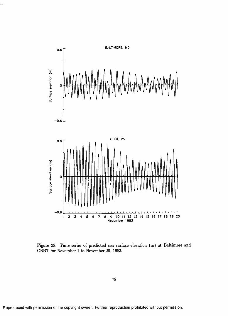
BALTIMORE, MD0.6

NEco

0)uo3LO

- 0.6

CBBT, VA0.6

««—NEcoo>JU0)

k-3(/)

- 0.61 2 3 4 5 6 7 8 9 10 11 12 13 14 15 16 17 18 19 20

November 1983

Figure 28: T im e series of predicted sea surface elevation (m) at Baltim ore and CBBT for November 1 to November 20, 1983.

78


m ain features can be pointed out. Spring tide occurs around November 5 when the

high tide reaches its m axim um while neap tide occurs around November 15 when

the high tide reaches its m inim um . A t CBBT, the tide is m ainly sem i-diurnal while

in Baltim ore the tide is mixed m ainly semi-diurnal, which is typical of the lower and

upper Bay (Fisher, 1986).

A first tria l of tidal circulation modeling was undertaken using the MU circula

tion model (Eqs. 1, 2, 3). The wind stress was set equal to zero and the quadratic

bo ttom stress was considered w ith a typical constant drag coefficient of 0.002 which

would be an average value for th e Chesapeake Bay (Section 3.2). T he circulation in

the Bay was forced a t the Bay m outh by imposing the predicted surface elevation

based on the harm onic constants a t the Chesapeake Bay Bridge Tunnel. Modeled

and predicted surface elevation (Fig. 29) show poor agreem ent, especially in the

upper Bay where modeled low and high tide am plitudes are sm aller than the cor

responding predicted tide. A comparison between modeled M 2 coam plitude and

cophase charts (Figs. 30 and 31) and the corresponding charts from Fisher (1986)

(Fig. 3) indicates th a t the discrepancy between modeled and observed tidal am

plitudes increases towards the upper Bay. Furtherm ore, the modeled M 2 tide

propagates slightly faster than the observed M 2 tide in the entire Bay. As a remedy

to the discrepancy, one could th ink to decrease the drag coefficient. Decreasing the

drag coefficient would indeed increase the am plitude of the tide and also change the

phase lag. The question is then how much can the drag coefficient be decreased to

m atch phase and am plitude of the M 2 tide everywhere in the Bay. One should also

realize th a t the adjustm ent of the drag coefficient to m atch the M 2 tide would not

necessarily lead to a m atch of the am plitude and phase of the o ther four constituents

(Crean et al., 1988). The tuning of the drag coefficient can quickly become very

tedious.

An analysis of the relative average error (Eq. 23) com puted over 24 hours for

79


BALTIMORE. MD0.4

-0.4

CAMBRIDGE, MD0.4

-0.4

SOLOMONS IS. MD0.4

§ -0.4 -a<o2 04 I5 o

LEWIS ETTA, VA

-0.4 L

KDTOPEAKE, VA0.6

-0.6

CBBT, VA0.6

-0.62 3 4 5 6 7 8 9 10 11 12 13 14 15 16 17 18 19 20

November 1983

Figure 29: Tim e series of modeled (dotted line) and predicted (solid line) surface elevation (m) a t six representative perm anent tide gauge stations. The drag coefficient was taken as cd = 0.002. Note the change of scale for the last two stations.

80


).3S

38*40' N

< 0.16

0.4

0.45

0.4

37*40' N0.45/ 0.5fo.55/0.6,

0.8,

0 6

[1.2'

36*40' N

75*30' W77*30'W 76*30'W

Figure 30: Coam plitude lines of the modeled M 2 tide expressed in feet.

81


38-40 N

360

35037-40' N

320

280

36°40'N75“30‘ W77°30'W 76°30' W

Figure 31: Cophase lines of the modeled M 2 tide expressed in degrees.

82


November 1 to November 19 (Table 4 and Appendix C) between m odeled and pre

dicted elevation shows an increase from a few percents in the lower Bay to about

15% in the upper Bay with a m aximum in the Potom ac river where th e maximum

relative error reaches a value of 24.3% a t Colonial Beach. This variation in the

relative average error from the lower Bay to the upper Bay would suggest a spatial

dependency of the drag coefficient. A strong fluctuation of the relative average in

tim e is also noted. For example, the error a t Baltim ore drops from a m axim um of

20.7% on November 6 to a minimum of 10.7% on November 17.

T im e and spatial dependence of the bottom drag coefficient was then taken

into account in the following recovery experim ent. A drag coefficient defined by

Eq. 5 was chosen and the param eters 1 /n and a were optim ally estim ated using the

variational technique described previously. W hile those param eters are constant,

the bottom drag coefficient is a function of space through its dependence in H ,

the to ta l water depth. The tim e variation of the drag coefficient was introduced by

evaluating the param eters for a period of one day for eighteen consecutive days which

includes one spring and one neap tide. The actual recovery started on November

2, 1983 through November 19, 1983 while the recovery for November 1, 1983 was

only used to initialize the procedure. Once the bottom drag coefficient param eters

were estim ated, the direct model was run for 24 hours w ith the new param eters in

order to initialize the circulation for the following day and compare modeled and

predicted elevations.

4.2.2 Recovery

For each day of the recovery experim ent, the initial guesses for the param eters 1 /n

and a were taken as their estim ated values from the previous day. The assimilation

process was stopped when the normalized norm of the gradient of the cost function

reached the value of 10-6 . This convergence criterion has been determ ined from the

83


results of November 1 and corresponded to the m inim um value th a t the normalized

norm of the gradient of the cost function could a tta in . For the period under study,

convergence occurred after 9 to 18 iterations and th e cost function decreased an

order of m agnitude. This small decrease in the cost function is due to the fact th a t

the initial cost function was already small since the recovery was s ta rted w ith the

best initial guess.

Predicted and modeled tidal elevations for six typical perm anent and six typical

comparison tide gauge stations are shown in Figs. 32 and 33, respectively. A sum

m ary of the root-m ean square error, relative average error and correlation coefficient

com puted using Eqs. 22, 23, 24 is given in Table 4 while values for each day between

November 2 and November 19 are given in Appendix C (Tables 6 to 11). Modeled

elevations with the estim ated drag coefficients show an excellent agreement with the

predicted elevations not only at the perm anent stations but also a t the comparison

stations. In general, the estim ated low tide am plitudes are slightly smaller than

the predicted am plitudes in the lower Bay. On the o ther hand, th e recovered high

tide am plitudes are slightly higher than the predicted am plitudes in the upper Bay.

However, differences between modeled and predicted elevation are of the same order

of m agnitude as th e m easurem ent errors for the entire Bay. A m axim um of less

than 7% for the relative average error (Table 4) is found in the m ain stem while the

relative error in the Potom ac river (Colonial Beach) reaches a m axim um of 9.86%.

Moreover, the variation between spring tide and neap tide in the relative error th a t

was found with a constant uniform drag coefficient is greatly reduced (Figs. 34, 35

and Appendix C). A correlation coefficient larger th an 0.96 is found in the m ain

stem and a m inim um correlation coefficient equal to 0.91 is found in the Potom ac

river. This indicates a very small shift between modeled and predicted elevations,

which could result from the fact th a t modeled elevations have been linearly in ter

polated in space to the location of the tide gauge. Finally, it should also be pointed

84


November 2 to November 19, 1983

Station Name rm s error (cm) relative error (%) correlationM in. Max. Mean Min. Max. Mean Min. Max. Mean

Havre de Grace, MD 2.4 11.8 7.31 1.73 16.90 9.70 0.955 0.990 0.9732.8 9.1 6.48 2.16 6.15 4.73 0.958 0.986 0.970

Baltim ore, MD 3.3 7.6 5.48 10.66 20.74 15.89 0.936 0.977 0.9652.1 4.6 3.11 1.67 6.47 3.92 0.951 0.989 0.975

Annapolis, MD 1.7 6.4 4.13 4.54 17.73 11.33 0.969 0.985 0.9751.1 4.6 2.65 0.93 7.03 3.43 0.979 0.996 0.989

Cam bridge, MD 4.5 9.8 7.16 8.94 17.16 13.78 0.945 0.996 0.9743.4 4.0 3.80 1.85 6.71 3.53 0.956 0.995 0.979

Solomons Is, MD 2.5 7.4 4.76 7.01 16.30 10.97 0.961 0.988 0.9762.0 4.9 3.25 2.09 5.38 4.07 0.962 0.992 0.983

Lewisetta, MD 1.9 6.7 4.10 3.30 11.32 6.76 0.985 0.997 0.9931.2 5.1 3.03 0.96 4.55 2.72 0.988 0.998 0.993

Gloucester P t, VA 2.6 12.5 7.29 1.79 10.44 5.87 0.971 0.997 0.9851.6 7.3 4.31 0.62 2.92 1.73 0.989 0.999 0.995

Kiptopeake, VA 3.4 8.4 5.26 0.97 3.41 2.32 0.976 0.999 0.9932.9 4.1 3.47 0.54 2.51 1.11 0.976 1.000 0.993

H am pton Roads, VA 2.9 11.0 6.51 2.01 7.36 4.26 0.990 0.998 0.9942.7 7.4 4.73 1.44 2.92 2.05 0.988 0.999 0.996

CBBT, VA 2.3 5.8 3.72 0.40 1.85 1.17 0.983 0.999 0.9952.9 4.4 3.49 0.60 2.25 1.09 0.980 1.000 0.994

B etterton, MD

M atapeake, MD

Avalon, MD

Chesapeake Bch, MD

Colonial Bch, VA

Holland Bar Lt, MD

Guardshore, VA

R appahannock, VA

New P t C om fS h, VA

2.4 10.9 6.972.1 6.4 4.371.9 6.4 4.131.5 4.3 2.723.2 8.6 5.482.1 5.4 3.541.6 5.5 3.461.6 4.9 3.133.5 12.2 7.772.9 9.6 6.082.4 6.8 4.312.0 4.7 3.223.8 10.5 6.703.0 6.6 4.773.0 6.2 4.153.1 4.3 3.612.6 8.2 5.202.3 5.2 3.67

2.78 19.65 11.671.72 4.04 2.853.86 14.15 9.031.71 4.57 2.761.34 14.34 8.561.36 4.95 2.952.80 11.45 6.992.35 6.09 3.996.59 24.29 15.583.77 9.86 6.723.09 8.81 5.701.72 3.24 2.523.27 8.06 5.321.41 3.14 2.202.50 5.57 4.391.83 5.07 3.071.38 5.36 3.491.03 2.07 1.58

0.970 0.996 0.9820.983 0.994 0.9900.962 0.995 0.9780.986 0.996 0.9930.955 0.994 0.9830.964 0.998 0.9850.971 0.997 0.9850.984 0.998 0.9930.924 0.976 0.9500.910 0.968 0.9390.966 0.995 0.9850.974 0.998 0.9910.967 0.992 0.9820.973 0.991 0.9830.950 0.995 0.9780.958 0.998 0.9830.979 0.997 0.9910.988 0.998 0.994

Table 4: M inimum, m axim um and mean value of the root-m ean square error (cm), the relative average error (%) and the correlation coefficient for November 2 to November 19,1983. T he first ten stations are the perm anent stations while the last nine are the comparison stations.

85


BALTIMORE, MD0.4

-0.4

CAMBRIDGE, MD0.4

-0.4

SOLOMONS IS, MD0.4

ss03>4>0>

1■e9

-0.4

LEWIS ETTA, VA0.4

-0.4

KIPTOPEAKE, VA0.6

- 0.6

CBBT, VA0.6

- 0.62 3 4 5 6 7 8 9 10 11 12 13 14 15 16 17 18 19

November 1983

Figure 32: Tim e series of m odeled (dotted line) and predicted (solid line) surface elevation (m) a t six perm anent tide gauge stations. Note the change of scale for the last two stations.

86


BETTERTON, MD0.6

- 0.6

CHESAPEAKE BCH, MD0.6

- 0.6

HOLLAND BAR LT.MD0.6

/•—sag -0.6>a>

H 0 6 I

GUARDSHORE, VA

- 0.6

RAPPAHANNOCK, VA0.6

- 0.6

NEW PT COMF SH, VA0.6

- 0.62 3 4 5 6 7 8 9 10 11 12 13 14 15 16 18 20

November 1983

Figure 33: T im e series of modeled (dotted line) and predicted (solid line) surface elevation (m ) a t six comparison tide gauge stations.

87


20

10

0

20

10

0

20

g 10h.g

o

BALTIMORE, MO

CAMBRIDGE, MD

SOLOMONS IS, MD

200)>o0)>

LEWISETTA, VA

10o0)0£

20

10

0

20

10

0

KIPTOPEAKE, VA

CBBT, VA

2 3 4 5 6 7 8 9 10 11 12 13 14 15 16 17 18 19November 1983

Figure 34: Tim e series of relative average error (%) for recovered (solid line) and modeled (cp = 0 .002) (dotted line) surface elevations a t six perm anent tide gauge stations.

88


20

10

0

20

10

0

BETTERTON, MD

CHESAPEAKE BCH, MD

20 HOLLAND BAR LT, MD

10

vcn

20 GUARDSHORE, VA

10

20

10

0

20

10

0

RAPPAHANNOCK. VA

NEW PT COMF SH, VA

2 3 4 5 6 7 8 9 10 11 12 13 14 15 16 17 18 19Novem ber 1983

Figure 35: T im e series of relative average error (%) for recovered (solid line) and modeled (c£> = 0 .002) (dotted line) surface elevations a t six comparison tide gauge stations.

89


out th a t the same agreement is found at Havre de Grace despite the fact th a t the

sta tion is near the Susquehanna river which has the biggest discharge of all rivers.

Using harm onic analysis for the tim e series of the modeled elevations with the

estim ated drag coefficients between November 2 and November 19, the am plitude

and phase of the M 2 and K \ tide a t every grid point of the m odel domain were

com puted. A comparison between the M 2 coam plitude chart from Fisher (1986)

(Fig. 3) and the corresponding chart for the modeled M 2 (Fig. 36) shows a very

good agreem ent. Same agreem ent (not shown) was found for the K \ tide. The

M 2 coam plitude lines run across the Bay a t the entrance, then become longitudinal

and finally run across the Bay in the upper Bay. The M 2 am plitude decreases

from the Bay m outh towards the m ain stem , and then increases north of Baltimore.

The am plitude of modeled M 2 tide is slightly larger than the am plitude found by

Fisher (1986), which can be a ttribu ted to the fact th a t the tim e series of modeled

elevations (18 days) was too short to fully separate the M 2, N 2 and S2 tides. A

comparison between the M 2 cophase chart from Fisher (1986) (Fig. 3) and modeled

M 2 cophase chart (Fig. 37) again shows excellent agreement. For example, the

310 degree cophase line goes through Rappahannock in both cases. The cophase

lines are uniformly spaced in the lower Bay. In the upper Bay, the cophase line

spacing decreases in the narrow portions and increases in the wider portions. The

fact th a t the curvature of the recovered cophase lines a t the entrance of the Bay is

not as pronounced as the curvature found by Fisher (1986) is due to the imposed

boundary condition at the Bay m outh. The predicted elevation was taken uniform

a t the Bay m outh which does not allow any curvature of the cophase lines. Two

v irtual am phidrom ic points, i.e., near the Severn river (north of Annapolis, Fig.

12) and the Potom ac river, are evident. At those locations, the coam plitude lines

are concentric and the cophase lines converge. Those two points were also found by

Browne and Fisher (1988).

90


39“40'N

38-40'N

>.65\0.7

,1.0

0.S'37“40' N

1.2 ,

u]

36-40' N

75-30'W

Figure 36: Coam plitude of the recovered M 2 tide expressed in feet.

91


M10,38’40'N

Mg.

33037°40' N

310300

360

250.

36°40N

77°30'W 76°3.0'W 75°30' W

Figure 37: Cophase of the recovered M 2 tide expressed in degrees.

92


W hile predicted and modeled elevations are in excellent agreem ent, probably the

m ost interesting feature to note is the periodicity of the estim ated inverse M anning’s

roughness and therefore of the bo ttom drag coefficient. As shown in Fig. 38, the

bo ttom drag coefficient decreases during spring tide (day 5-6) and increases during

neap tim e (day 14-15). The exponent a (Eq. 5) is m ainly constant during the entire

period.

The difference between spring and neap tide values is larger in th e regions with

a depth less than 10 m. The estim ated bottom drag coefficient varies between

2.5 x 10 4 and 3.1 x 10 3. The lower value is smaller than the values found in the

classical tidal modeling literature (Ronday, 1976; W erner and Lynch, 1987; Crean et

al., 1988). However, using an inverse m ethod and tidal-current observations in the

lower and upper Bay, Bang (1994) found a similar range of values for the bottom

drag coefficient, i.e., 2.0 x 10“4 < cd < 1.6 x 10-3 . Discussion of the eventual causes

of the periodicity of the drag coefficient can be found in Section 5.

4.3 Wind-driven circulation

Since modeled tidal circulation in the Bay has shown to be considerably improved

by using variational da ta assimilation, our next focus is on w ind-driven circulation

which is even harder to model. Indeed, the surface forcing, i.e., th e wind stress,

is poorly known for the Chesapeake Bay since the wind observations are available

only a t the m ajor airports and do not necessarily represent the wind over the water.

As m entioned in Section 3.6, the goal of the present experim ent is to estim ate

the bottom drag coefficient, the wind stress components at four locations and the

hourly surface elevations a t the open boundary during the assim ilation process and

get the best representation of the wind-driven circulation in the Bay. As for the

tidal circulation study, the assim ilation period is in November. However, in order

to have wind observations to compare to the estim ated wind using the variational

93


0.0040

0.0030

2 m

VOug> 0.0020TJEo

3 m

4 m

S mO

CD

m0.0010

0.000015 205 10

November 1983

Figure 38: Tim e series of estim ated bottom drag coefficient cp for depths between 2 and 50 m.

94


assim ilation technique, the year 1990 had to be considered instead of the year 1983.

Observations and results of the assim ilation process are described in the next two

subsections.

As additional evidence of the improvem ent of the modeled wind-driven circula

tion by using d a ta assimilation, two days in Septem ber 1983 when da ta are available

a t m ore tide gauges than the one used for assim ilation were also considered. Hence,

it was possible to compare m odeled elevations with observations which were not

assim ilated. Unfortunately, during th a t period of tim e, wind speed and direction

was only m easured at the airports. The results of th a t experim ent is presented in

the last subsection.

4.3.1 Observations

W ind-driven circulation in the Chesapeake Bay was investigated by assimilating

hourly sea surface elevation observations from ten perm anent tide gauges (Fig. 12)

betw een November 2 and November 8,1990. As in the tidal circulation experiment,

observations of November 1 are used to initialize the recovery process. During tha t

period of tim e, hourly wind speed and direction observations were available a t two

buoys deployed by NOAA (Fig. 12), Thom as Point and Chesapeake Light Tower,

and at the tide gauge station CBBT. A comparison between observed and estim ated

wind was therefore possible.

T im e series of predicted using th e harm onic constants from Fisher (1986) and

observed sea surface elevations a t two perm anent tide gauge stations, Baltimore

and CBBT, are plotted in Fig. 39 for November 1 through November 10, 1990.

Differences between predicted tidal and observed elevations are noticeable during

those few days, which suggests th a t the wind plays an im portan t role. During the

chosen assim ilation period, either a southwesterly or southeasterly wind (Fig. 40)

persisted for about four days over the entire Bay with a speed less than 5 m /s in

95


o.8 rBALTIMORE, MD

CBBT, VA

November 1990

Figure 39: Tim e series of predicted tidal (solid line) and observed (dotted line) elevation in Baltim ore and CBBT for November 1 to November 10, 1990.

96


the upper Bay and slightly higher in the lower Bay. During those few days, a sea

breeze pattern is also noticeable. In the afternoon of November 5, the wind speed

increased to about 10 m /s in the upper Bay. An increase of the surface elevation is

im m ediately noticeable in the upper Bay, e.g., th e high tide elevation is about twice

its predicted value a t Baltim ore. A smaller change in the surface elevation can also

be seen at CBBT. On November 6 , a change of th e wind direction associated with

the passage of a cold front, is evident. The wind becam e northw esterly in the upper

Bay and northeasterly in the lower Bay. Again, a sim ilar eifect of the wind direction

change can be seen in th e observed surface elevation a t both stations. The surface

elevation decreased in Baltim ore and increased a t CBBT, which is the expected

response to a northw esterly and a northeasterly wind, respectively. This change

in the surface elevation is larger on November 8 when the wind become stronger.

Finally, notice th a t the wind direction outside of th e Bay (Chesapeake Light Tower)

is roughly the same at CB BT while the wind speed is slightly larger. Therefore,

we do not anticipate any different behavior in the surface elevation from the Bay

m outh and a t CBBT.

The tim e variations of the wind stress and the bottom drag coefficient were in tro

duced in the recovery experim ent by evaluating the param eters for a period of one

day for seven consecutive days. The actual recovery started on November 2 through

November 8, 1990 while the estim ated param eters for November 1, 1990 were only

used to initialize the procedure. Once the bo ttom drag coefficient param eters, wind

stress and boundary conditions were estim ated, the direct model was run for 24

hours with the new param eters in order to initialize the circulation for the following

day and compare modeled and predicted elevations.

97


Reproduced

with perm

ission of the

copyright ow

ner. Further


without

permission.

15lO5

N

-lO-15

Thomas Point

x h \

15lO5O

-5-lO-15

y 5 m/sCBBT

tooo 15lO5

— N

-5-lO-15

IS m/s

V i z / f a .

Chesapeake Light Tower

November 1990

Figure 40: H ourly observed w ind in N ovem ber 1990 a t two buoys, Thom as P o in t and Chesapeake Light Tower, and a t the tide gauge s ta tio n C B B T . T he stick diagram is p lo tted using th e oceanographic convention.

4.3.2 Recovery

For each day of the assimilation experim ent, the initial guess for the control variables

was taken as their estim ated value from the previous day. Based on the recovery on

November 1, the recovery was stopped when the normalized norm of the gradient

of the cost function reached a value of 10-3 . The convergence criterion was set to a

higher value than for the tidal experim ents. The assimilated d a ta are indeed actual

observations and are noisier than the d a ta used in the tidal recovery. For each day

of assim ilation, the cost function decreased one order of m agnitude. As for the tidal

experim ent, the small decrease in the cost function can be a ttrib u ted to the fact

th a t the assim ilation runs were s tarted w ith the best initial guess. The num ber of

iterations necessary to satisfy the preset convergence criterion varied between 244

and 370. T he cost function decreased rapidly during the first 30 iterations and

continued to slowly decrease until convergence was reached. This p a tte rn was also

found for the twin experiments (Section 4.1).

T im e series of modeled sea surface elevation is shown in Fig. 41. T he relative

average error over 24 hours at six perm anent tide gauge locations is p lo tted in

Fig. 42. Root-mean square error, relative average error and correlation coefficient

(Eqs. 22, 23, 24) are given in Table 5 for every day of the assim ilation period.

Excellent agreement between estim ated and observed surface elevation is evident

for the entire period of assimilation in the lower Bay. In general, a relative average

of error less than 3% is found for the stations in the lower Bay and the correlation

coefficient is over 0.99. In the upper Bay, the agreement is also very good until the

frontal passage. The relative average error is less than 5% until November 6 when

it increases to about 15%. While the correlation coefficient is over 0.9, a variation

in its value is also noticeable for the same period.

Recovered wind vectors at Thomas point and CBBT for November 2 to November

8 , 1990 are plotted in Figs. 43 and 44, respectively. W ind speed and direction

99


BALTIMORE. MD0.6

- 0.6

CAMBRIDGE.0.6

- 0.6

SOLOMONS IS. MD0.6

g -0.6a>V« 0.68■g5a 0

LEWISETTA, VA

- 0.6

KIPTOPEAKE, VA0.8

- 0.8

CBBT, VA0.8

- 0.82 83 5 6 74

November 1990

Figure 41: Tim e series of modeled (dotted line) and observed (solid line) surface elevation (m) a t six perm anent tide gauge stations.

100


20

10

0

20

10

0

BALTIMORE. MO

CAMBRIDGE, MO

20 SOLOMONS IS, MD

o

LEWISETTA. VA

CE

KIPTOPEAKE, VA

4 CBBT, VA

2

075 64

Novem ber 1990

Figure 42: Tim e series of relative average error (%) between m odeled and observed surface elevation a t six perm anent tide gauges. Note the change of scale for the last three stations.

101


Station Name November 19901 2 3 4 5 6 7

Havre de Grace, MD 5.31.73

0.985

6.23.03

0.971

4.31.24

0.991

7.93.44

0.968

9.23.71

0.972

5.81.77

0.985

1.111.510.895

Baltimore, MD 4.03.78

0.976

4.54.46

0.983

4.13.61

0.990

5.54.46

0.986

7.55.71

0.976

9.514.290.937

8.016.430.897

Annapolis, MD 4.97.11

0.970

2.01.03

0.990

2.41.44

0.994

2.10.91

0.991

3.61.72

0.983

8.514.910.926

5.07.49

0.949

Cambridge, MD 6.04.82

0.986

3.81.56

0.994

3.71.45

0.994

5.02.58

0.994

4.82.14

0.988

11.213.640.930

11.216.470.943

Solomons Is, MD 3.93.40

0.974

2.61.26

0.990

2.20.91

0.992

2.91.73

0.987

4.43.53

0.978

5.45.02

0.960

5.89.21

0.957

Lewisetta, MD 2.20.92

0.992

2.30.85

0.995

1.90.55

0.996

2.40.89

0.995

4.53.15

0.987

3.82.48

0.982

3.32.58

0.984

Gloucester Pt, VA 4.10.92

0.992

4.00.82

0.994

3.80.65

0.994

3.40.48

0.996

2.80.35

0.997

6.52.13

0.985

5.51.93

0.982

Kiptopeake, VA 1.80.13

0.999

1.60.09

0.999

1.80.11

0.999

2.10.13

0.999

2.30.18

0.998

3.20.38

0.997

3.80.71

0.995

Hampton Roads, VA 3.50.63

0.998

4.10.79

0.997

4.20.73

0.997

3.60.50

0.999

3.00.36

0.998

5.31.32

0.995

5.61.84

0.986

CBBT, VA 2.30.22

0.999

3.10.33

0.998

3.10.30

0.998

2.70.22

1.000

1.90.12

1.000

3.00.34

0.999

3.50.61

0.996

Table 5: Root-mean square error (cm) (first number), relative average error (%) (second number), and correlation coefficient (third number) for the wind-driven experiment

102


were obtained from the wind stress components using a quadratic law with a drag

coefficient of 2.0 x 10“3 (Schwab, 1982). The wind pattern is well represented in

the lower Bay. At CBBT, the estimated wind is mainly southwesterly and shows

an increase of magnitude late on November 5. A change of direction occurs on

November 6, which is in agreement with the observed wind pattern. In the upper

Bay, the agreement is not as good until the frontal passage when the wind speed

increased to 10 m/s and a change in direction occurred. This would suggest that

during periods of weak wind, mechanisms other than the local wind forcing are more

important in the narrowest part of the Bay.

The recovered drag coefficient (Fig. 45) shows a minimum on November 5, which

corresponds to the period of spring tide. This is followed by an increase until

November 6 when there is a frontal passage. The drag coefficient then decreases

and reaches roughly the same value regardless of the depth of the considered region

in the Bay. While a continuous increase of the drag coefficient was expected until

neap tide, northwesterly and northeasterly winds seem to decrease the magnitude

of the drag coefficient compared to its value with no wind or southeasterly wind.

The last recovered control variable to examine is the boundary elevation at the

Bay mouth. As expected, the high tide elevation (Fig. 46) is higher and the low

tide is lower on the northern end of the Bay mouth than at the southern end. This

di (Terence in elevation decreased when the wind changed direction and blew from the

northwest and the northeast. The elevation at the northern end of the Bay mouth

is slightly higher than the expected value. This can be due to the fact that the

boundary region in our model is about half the width of the real boundary (Fig. 9).

103


Please Note

Page(s) not included with original material and unavailable

from au thor or university. Filmed a s received.

104

UMI


Reproduced

with perm

ission of the

copyright ow

ner. Further


without

permission.

001

Recovered5 mft

Observed

-5-10-IS

^ ( 5

4 5 6November 1990

.d l

Figure 44: Recovered and observed wind at CBBT. The recovered wind, plotted at the middle of the recovery day, is constant during that day.

0.0020

0.0015

? 0.0010

0.0005

0.0000 JLLL

2 3 5 76 84November 1990

Figure 45: November 1990 time series of recovered bottom drag coefficient cp for depths between 2 and 50 m.

10G


Figure 46: Tim e series of hourly boundary surface elevation (m) from the southern end to the northern end of the Bay m outh.

107


4.3.3 Further investigation of the recovery

In the previous wind-driven circulation experim ent, sea level was only m easured at

ten tide gauges and all the observations were used in the assim ilation process. In the

best case, one can expect that a t those ten stations there is no misfit between the

m odeled elevations obtained using the estim ated param eters and the observations.

Indeed, the assim ilation procedure is based on the m inim ization of the misfit be

tween m odeled and observed elevations. However, this does not guarantee no misfit

a t o ther locations in the Bay. In order to increase our confidence in the feasibility

of recovery of wind-driven circulation in the Bay, the previous recovery experiment

has been repeated for Septem ber 20 and September 21, 1983. During th a t period of

tim e, sea level measurem ents are also available a t tide gauges o ther than the per

m anent tide gauges. It was then possible to compare m odeled and observed surface

elevations from other tide gauges than the one used during the assim ilation pro

cess. Unfortunately, the wind observations are only available a t the m ajor airports

and comparison between estim ated and observed wind is very difficult. T im e series

of the predicted based on five m ajor constituents and observed elevations a t two

tide gauge stations, Baltimore and Chesapeake Bay Bridge Tunnel, are p lotted in

Fig. 47. During the considered period of tim e, a dom inant effect of the wind on

the surface elevation can be seen. One should also point out th a t a t the same tim e

there was a destratification of the Bay (Blumberg and Goodrich, 1990). Therefore,

the circulation during those two days should be well represented by our barotropic

model.

The modeled sea surface elevation with the estim ated bottom drag coefficient

is plo tted in Fig. 48. Modeled and observed surface elevations show a very good

agreement not only a t the perm anent but also comparison tide gauges. Furtherm ore,

the m agnitude and direction of the recovered middle Bay wind, i.e., southwesterly

wind, was found to be comparable to the wind measured at the Patuxent River Naval

108


o.8 rBALTIMORE, MD

CBBT, VA

21Septem ber 1983

Figure 47: T im e series of observed (dotted line) and predicted (solid line) elevation a t Baltim ore and CBBT from Septem ber 18 to Septem ber 24, 1983.

109


BALTIMORE, MD0.6

- 0.6

SOLOMONS IS, MD0.6

0.6

CBBT, VA0.6

sVg -0.6••sSs 06

1v) 0

FERRY COVE, MD

CHESAPEAKE BCH, MD0.6

RAPPAHANNOCK, VA0.6

20 21 22 September 1983

Figure 48: Septem ber 1983 tim e series of recovered (dotted line) and observed (solid line) surface elevation (m) a t three perm anent and th ree comparison tide gauge stations.

110


Air station (Blumberg and Goodrich, 1990). This experim ent indicates th a t the

modeled wind-driven circulation in the m ain stem can be improved by assimilating

only the surface elevations m easured a t the ten perm anent tide gauges.

I l l


5 Discussion

The previous sections presented the formalism, im plem entation and results of adjoint

variational assimilation of tide gauge observations in the Chesapeake Bay when the

dynam ical constraint is a 2-D vertically-integrated shallow w ater model. The follow

ing sections first describe the problem of identifiability and regularization in param

eter estim ation. The results of the data assimilation experim ents are then discussed

from two perspectives: first from the point of view of the assim ilation technique and

second from the improvement of the modeled circulation in the Chesapeake Bay.

There was no a ttem p t to improve the assimilation technique nor the circulation

model b u t rather to use those two tools and tide gauge observations to estim ate

the model control variables which could improve the modeled tida l and wind-driven

circulation in the Bay.

T he discussion of the identical twin experim ents focuses on the definition of

the cost function. This is followed by a discussion of the ra te and precision of the

recovery of the control param eters and boundary conditions when model generated

observations are subsampled. The results of the tidal and wind-driven circulation

experim ents are discussed w ithin the context of the physics of the Bay. Particular

a tten tion is given to th e estim ated bottom drag coefficient for tida l and wind-driven

circulation and to the recovered wind stress in the wind-driven circulation. Finally,

fu ture studies are indicated.

112


5.1 Identiiiability and regularization in parameter estimation

T he m ain problem in param eter estim ation comes from the identifiability of param

eters, especially when th e num ber of param eters is large. In general, identification

refers to the determ ination of unknown param eters such th a t the predicted response

of the model is close to the process observations. Banks and Kunish (1989) and

O m atu and Seinfeld (1989) addressed the question of identifiability of distributed

param eter systems and proposed performance criteria, e.g. least-squares perfor

m ance criterion (cost function). Due to the ill-posedness of the problem, regular

ization approach is often used which leads to a well-posed problem . The problem

of regularization has been defined by O m atu and Seinfeld as follows. Regularization

of a problem refers to solving a related system called the regularized problem , the

solution of which is m ore regular in a sense than th a t of the original problem , and

which approxim ates the solution of the original problem. Regularization is thus an

approach to circum vent lack of continuous dependence on the data. The regular

ized problem is a well-posed problem whose solution yields a physically meaningful

answer to the given ill-posed param eter estim ation problem (Kravaris and Seinfeld,

1985). Banks and Kunish (1989) pointed out th a t the addition of the regularization

term changes the natu re of the problem and th a t the solutions of the regularized

problem are different from those of the original problem. Adding a regularization

term to the fit-to-data criterion can, for instance, specify certain additional sm ooth

ness properties of the solution. Finally, experience with param eter estim ation shows

th a t severe difficulties arise when using unconstrained unregularized algorithms with

the adjoint approach to estim ate unknown param eters when the dimension of the

approxim ating s ta te is kept fixed while increasing dimension of approxim ating pa

ram eter spaces (Kunish and W hite, 1986; Yeh, 1986).

In th is study, the im portan t param eters to be estim ated were identified from

113


previous studies of the circulation in the Chesapeake Bay (Section 2). T he regu

larization approach consists in the use of penalty-regularization term s in the cost

function. The effect of the addition of a penalty term to the cost function is discussed

in the following section.

5.2 Data assimilation and twin experiments

First and forem ost, the identical twin experim ents provide insight into the feasibility

of param eter estim ation in the Chesapeake Bay, in the use of an appropriate cost

function, and in th e adequacy of the observations th a t are not contam inated with

observational errors.

5.2.1 Definition of the cost function

As m entioned in Section 3, variational da ta assim ilation consists of estim ating the

best value of the control param eters by minimizing a cost function which measures

the misfit between model results and observations. The main concern in param e

ter estim ation using variational da ta assim ilation is the adequacy of the type and

num ber of observations used to define the cost function. In his discussion of linear

regression as a paradigm of model fitting, Thacker (1987) showed th a t th e m ini

mum num ber of observations m ust be a t least as large as the independent model

variables. However, even if the num ber of observations is large enough, adequacy

of the d a ta is not guaranteed. Tziperm an et al. (1992a) showed th a t even though

the num ber of tem peratu re and salinity observations was larger than the num ber of

unknown wind stress components, those observations did not provide independent

information and therefore the convergence to the correct forcing was relatively slow.

They showed th a t adding surface velocity observations improved the convergence

to the correct wind forcing. Similar problems can arise from the discretization on

fine grids required to resolve the phenomenon under study. Indeed, the observations

114


m ight be too sparse in space and tim e to determ ine the gridded variables. Adding

observations is not always possible. A cure is to supplement the inadequate da ta

w ith prior knowledge or prejudice th a t the gridded values should be smooth. This

is equivalent to adding penalty term s to the cost function, which is defined as the

weighted square of the differences between model results and observations. As men

tioned in Section 3.6, Richardson and Panchang (1992) and Lardner et al. (1993)

showed th a t it was necessary to add a penalty term to the cost function in order to

assure smoothness of the estim ated field.

In this study, the identical twin experiments show th a t in order to recover a

sm ooth open boundary condition close to its real value, a term , Jp (Eq. 21), which

penalizes large variations of the surface elevation from one grid point to another

a t the boundary, need to be added to the cost function (Eq. 20). T he necessity

of the penalty term is evident even when there is a maximum of observations, i.e.,

d a ta a t every grid point. In that case, the num ber of observations is more than

ten tim es the num ber of unknown variables. This suggests th a t surface elevation

does not provide enough information about the boundary elevation, which can be

explained as follows. The exchange between the open ocean and the Bay through

the Bay m outh has a strong influence on the surface elevation in a lim ited area

of the lower Bay even though the signal generated at the boundary propagates

throughout the entire Bay. Furthermore, the elevations a t the Bay m outh have a

smaller phase lag w ith the elevation in the lower Bay than w ith the elevation in

the upper Bay. Therefore, the intensity of the signal from the boundary conditions

will be stronger in the surface elevation observations in the lower Bay than in the

upper Bay. This explanation is also supported by the distribution of the relative

average error between observations and recovered elevation after 15 iterations of

the assim ilation process (Figs. 17, 20, 23). After 15 iterations, when wind stress

components alm ost reach their true values, the effect of the boundary condition is

115


clearly seen in the lower Bay where the relative average error is larger than elsewhere

in the Bay.

Instead of penalizing the cost function, one could increase the window of assim

ilation to two days, for exam ple, which would result in an increase in the num ber

of observations. However, a larger window would not solve the problem since the

num ber of required boundary conditions will also increase. One could assim ilate

different types of observations, e.g., current velocities. This is not possible in the

Chesapeake Bay since the current is not routinely m easured. The addition of the

penalty term thus seems the most appropriate for our study.

5.2.2 Scaling of the control variables

The second concern in the variational m ethod comes from the use of non-linear

optim ization, such as the lim ited memory quasi-Newton m ethod. The control vari

ables often differ by several orders of m agnitude and the scaling of those variables

has been shown to be im portant in order to accelerate the convergence. Discussion

of the role of various scaling techniques in improving the performance of descent

algorithm s can be found in Gill et al. (1981), Navon and de Villiers (1983). Seiler

(1993) showed th a t it is im portant to have the right scaling of the control variables

otherwise the optim ization m ight fail to converge, indeed yield senseless param e

ters. In this study, scaling similar to the one used by Navon et al. (1992a) was

applied. This scaling (Section 3.6) brings all the control variables to the same order

of m agnitude. The only unknown param eter, two orders of m agnitude larger than

the other param eters, is the inverse of the M anning’s roughness. Dividing it by a

factor 100 is the simplest way of bringing all the param eters to the same order of

m agnitude (Section 3.6). However, when scaling of the inverse of the M anning’s

roughness param eter is applied, the true value of the param eters is not recovered.

On the o ther hand, good results in an acceptable num ber of iterations was obtained

116


without scaling of the param eters. In that case, wind stress components are first

adjusted followed by th e drag coefficient param eters and finally the boundary ele

vations. For this study, scaling of the largest param eter does not help the recovery

process and therefore is not used. Investigation of different scalings of the control

variables was beyond the scope of the study. B ut, th a t problem needs to be ad

dressed in a fu ture study, especially when the num ber of param eters is larger than

in the cases trea ted here.

5.2.3 Rate and precision of the recovery

The ra te and precision a t which the control variables are recovered in the twin

experiments clearly show a dependence on the availability of observations. Over

the past several decades, only ten perm anent tide gauges (Section 2 and Fig. 12)

have been deployed in the Chesapeake Bay. Most of those tide gauges are situated

in embaym ents or entrances to rivers. It is, however, very encouraging to see th a t

even w ith lim ited observations, i.e., with hourly surface elevation observations a t

ten stations, it is possible to recover, to two significant figures, the bottom drag

coefficient param eters, the wind stress components a t four locations in the m ain

stem while boundary conditions are recovered to 85% of their tru e values. For

all the twin experim ents, the wind stress components are first recovered, which

indicates th a t the wind stress is the dom inant forcing in the circulation model. As

previously m entioned, th e lack of recovery of the boundary conditions to their true

values can be due to the fact th a t the signal from the boundary is strong only in

the surface elevation m easured at the tide gauges in the lower Bay. In addition,

the num ber of tide gauges near the Bay m outh (Fig. 12) is ra ther small. Indeed,

only two stations, CBBT and Kiptopeake are in the m ain stem while two other

stations, H am pton Roads and Gloucester, are located ear the Bay m outh in the

entrance to rivers. T he surface elevation at the la tte r two stations would also reflect

117


th e effect of the river discharge, of the geometry of the rivers and of bottom and

surface stresses, which are probably m ore im portant than the effect of the boundary

conditions. A way of increasing the im portance of the boundary elevation signal

during th e recovery would be to weight differently the d a ta misfit between modeled

and observed elevations from the lower Bay Proper stations in the cost function.

In this study, there was no a ttem p t to give more weight to those observations to

com pute the cost function which could lead to a b e tte r recovery of the boundary

condition. The boundary is indeed arbitrarily taken some distance from the Bay

m outh and is also narrower than the real opening a t th a t distance. Therefore, we

are not interested in the recovery of the boundary condition itself bu t in an estim ate

of th e boundary condition which would be physically acceptable and lead to the best

circulation in the Bay.

5.3 Data assimilation and Chesapeake Bay

W hile the identical twin experim ents guide us on the rate of recovery of the control

variables, the appropriate density of da ta , and the definition of an appropriate cost

function, da ta assim ilation using tidal elevations (Section 4.2) and real observations

(Section 4.3) gives some insight into the physics of the Bay and some empirical

quantities used in the model, such as the bottom drag coefficient. Indeed, these

results indicate th a t the bottom drag coefficient displays a periodicity corresponding

to the spring-neap tide cycle and its value is a function of the wind speed and

direction. The results also confirm W ang’s (1979a,b) findings th a t the response to

the wind is different in the lower and upper Bay.

5.3.1 Estimate of the bottom stress and drag coefficient

During the past decades, the bottom stress in tidal models has been defined as

a quadratic law with the bottom drag coefficient being determ ined empirically to

118


m atch the am plitude and phase of the observed m ajor tidal constituents. For exam

ple, in their study of the coastal seas of southern British Columbia and W ashington

States, Crean et al. (1988) found it necessary to vary spatially th e bottom drag

coefficient. The overall friction was taken equal to 0.003, with different values (0.03

or 0.006) in the Puget Sound and various stra its and passages. In the modeling of

tidal m otion in the English Channel and southern part of the N orth Sea, a constant

bo ttom drag coefficient was taken equal to 2.32 x 10-3 (Werner and Lynch, 1987;

Ozer and Jam art, 1988). Mofjeld (1988) showed th a t the quadratic coefficient re

lating the bottom stress to the vertically averaged velocities depends explicitly on

th e w ater depth and found th a t it can be related to the ratio H /z 0 where z0 is the

bo ttom roughness and H the to ta l water depth. Based on the non-rotating channel

theory in which frictional drag balances barotropic pressure forcing and shear pro

duction of turbulence is balanced by local dissipation (closure of level 2), Mofjeld

(1988) found th a t the bo ttom drag coefficient is given by

K2CD = (25)

K > -

where k = 0.4 is the von K arm an constant.

Using a variational d a ta assimilation technique and tidal elevations, Lardner et

al. (1993) estim ated the bottom drag coefficient for the Arabian Gulf. The drag

coefficient was defined as g /c 2 where c = C log(/i) is the Chezy coefficient, h the

undisturbed depth of the w ater, and g is the acceleration due to gravity. They found

in general a higher value for C than the em pirical value of 25 used in a previous

tidal model for the sam e region (Lardner et al., 1982). Using an inverse m ethod

and tidal-current m easurem ents in the Chesapeake Bay, Bang (1994) found values

between 2.0 x 10-4 and 1.6 x 10-3 . Note tha t all the mentioned studies consider only

a spatial variation of the drag coefficient. The tem poral variation was not taken into

account in 2-D m odeling of tidal and wind-driven circulation.

119


• Temporal variation o f the bottom drag coefficient

In our study, the bottom drag coefficient was defined in term s of a Chezy coef

ficient, i.e., it depends on the total depth, and a roughness coefficient called M an

ning’s roughness (Eq. 5). A system atic ad justm ent of the drag coefficient was done

by assim ilation of tidal elevations and estim ation of the two free param eters, i.e.,

the exponent of the to ta l depth and the inverse of the M anning’s roughness. In

the tidal experim ent, by assimilating the predicted tidal elevation on 24 hours for

19 consecutive days, tem poral variation of th e drag coefficient for a spring-neap

tide cycle was allowed. Furtherm ore, the spatial variation was taken into account

through the dependence of the coefficient on th e to ta l depth. As results of tidal

elevations assim ilation in the Chesapeake Bay, it is found th a t the bottom drag

coefficient displays a periodicity corresponding to the fortnightly m odulation. The

drag coefficient varies between 2.5 x 10-4 and 3.1 x 10-3 with a m inim um value a t

spring tide and a m axim um a t neap tide. W hile the lower value seems to be smaller

than the value found in the literature related to tidal modeling (Johns, 1983; Crean

et al., 1988; Ozer and Jam art, 1988), a sim ilar range was found by Bang (1994) in

his study in the Chesapeake Bay. The fortnightly m odulation is m ainly found in the

M anning’s roughness while the exponent rem ains close to 1 /6 , the value commonly

used in estuary studies (Officer, 1975).

The first plausible cause for the tem poral variation of the drag coefficient can

be a ttribu ted to the variation of the bo ttom roughness. Indeed, several studies

(McCave, 1973; Taylor and Dyer, 1977; G rant and M adsen, 1982; Davies, 1983;

Gross and Nowell, 1983; Wright et al., 1992) showed tem poral variability of the

bottom drag coefficient due to variation in roughness elem ents such as ripples and

biogenic micromorphology, in movable bed roughness caused by sedim ent transport

and in interactions between waves and currents. Although the tem poral changes of

the bottom roughness in the Chesapeake Bay are not yet well understood, W right

120


et al. (1992) found seasonal variability due to biological processes controlling bed

micromorphology and variation a t period of a few hours due to wave activity.

A second cause which would account for the periodicity of the bottom drag coef

ficient can be related to the level of stratification. In their study of the Rhine regions

of freshwater influence, Visser et al. (1995) showed th a t the constituents of the tidal

currents depend not only on tidal forcing a t astronom ic periods but also on the less

predictable stratification and destratification processes and questioned th e robust

ness of the standard tidal analyses. It has been shown th a t mixing in the lower

Chesapeake Bay and tribu taries appears m ost intense a t spring tide while s tra ti

fication appears m ost highly developed a t neap tide (Haas, 1977; Valle-Levinson,

1995). A t spring tide, the vertically averaged current and the bottom current are of

the same order of m agnitude while the vertically averaged current is sm aller than

the bottom current a t neap tide. Since the bottom stress in our model is defined in

term s of the vertically averaged current, the drag coefficient m ust be larger during

neap tide th an during spring tide in order to com pensate the difference between

averaged and bottom current assuming th a t the bottom drag is the same.

By adjusting the drag coefficient spatially and tem porally, the sim ulation of the

tidal circulation in the Chesapeake Bay is improved. Com parable results were found

by Lardner et al. (1993) in the A rabian Gulf. However, the periodicity of the drag

coefficient was not taken into account. As a consequence, the rms error found by

Lardner a t various stations in the Gulf is higher during spring tide than neap tide

(see Fig. 49) which would lead to the proposition th a t a tem poral variation of the

drag coefficient is not only true for the Chesapeake Bay, but also for o ther bodies

of water.

Finally, using Eqs. 5 and 25 and an average depth of 8 m , the bottom roughness

is found to be equal to 0.01 cm during neap tide which is in good agreem ent with

the value found by W right et al. (1992). During spring tide, the bottom roughness

121


AFTER OPTIMIZATION — BEFORE OPTIMIZATION ------

0.05

DAY

DAY

RMS ERRORS AT ARBY

RMS ERRORS AT ABUS

RMS ERRORS AT SFPL

OAY

Figure 49: R oot-m ean square errors a t sta tions in the A rabian Gulf for 100 days following the beginning of the assim ilation period. T he errors are shown before (dotted line) and after (solid line) optim ization. (Lardner et al., 1993).

122


value averages 0.001 cm which is slightly too small. In order to get a more accurate

estim ate of the bo ttom roughness, the relation (25) should be used in the circulation

m odel and z0 be estim ated during the assimilation process.

• W ind effects

The study of wind-driven circulation shows th a t the bottom drag coefficient

decreased during strong northeasterly and northwesterly wind compared to its value

w ithout wind or with a weak wind (Figs. 38, 45). Again, the decrease can be related

to the level of stratification and changes in the bottom roughness. During frontal

passage, the w ater column becomes less stratified, indeed destratified (Blumberg

and Goodrich, 1990). Therefore, bottom velocity and vertically averaged velocity

approach the same value. Furtherm ore, W right et al. (1992) argued th a t strong

winds should be able to generate 5-s waves large enough to agitate the bed a t depth

of 10 to 12 m in the Bay and yield variation in the bottom roughness.

Similar wind effect on the bottom friction was found by Ronday (1976) for his

study of the N orth Sea. He showed th a t a term proportional to the wind stress had

to be subtracted from the bottom stress in order to m atch modeled and observed

elevation when the drag coefficient was taken equal to its value w ithout wind. For a

northeasterly wind, this corresponds to an increase of the bottom stress which can

also be achieved by a decrease of the bottom drag coefficient.

5.3.2 Atmospheric forces in the Bay

T he second im portan t feature noticed during the wind-driven circulation experim ent

is th e relative im portance of the driving forces in the Bay. W hile the modeled surface

elevation is in excellent agreement with the observed elevations in the m ain stem , the

estim ated wind speed and direction in the upper Bay are not in as good agreement

w ith the observations as in the lower Bay. Thom as Point buoy, which is situated

123


a t the narrowest portion of the Bay (Fig. 12) was used to com pare the modeled

results with the observations in the upper Bay and C B B T tide gauge station was

used in the lower Bay. Near Thom as Poin t, the main stem changes its orientation

from northwest-southeast to northeast-southw est and becom es shallower (Fig. 1).

Then, during periods of weak wind, th e topographic and narrow ing effect should be

dom inant. The model grid spacing, roughly 2 km, is probably too large to correctly

resolve the influence of the narrowing of the Bay. Instead, th e correction is done to

the wind stress in order to minimize th e d a ta misfit a t A nnapolis which is the closest

tide gauge station. When the wind becom es stronger, as in th e case during a frontal

passage, the surface elevation response to the wind is larger and the wind signal in

the observations is also stronger. In those conditions, estim ated and observed wind

speed and direction are in excellent agreement. Further investigation with a finer

grid than 2 km is needed to fully investigate the circulation in th a t area.

A second effect that is neglected and could be a cause for the disagreement

between estim ated and observed wind is the inverted barom eter effect, which induces

an increase of the surface elevation for a low pressure system and a decrease of the

surface elevation for a high pressure system . For example, Paraso and Valle-Levinson

(1995) showed th a t for 10-11 February 1992, the barom etric pressure rise contributed

57% to the sea level change at CBBT and in general the effects of the atmospheric

pressure on sea level are not negligible. Vieria (1986) found th a t the 2-2.5 day sea

level oscillations in mid-Bay could n o t be identified w ith a seiche in the Bay but

could be due to the atmospheric pressure. During the period corresponding to our

study, changes in the barometric pressure are also im portan t. From November 1 to

November 3, 1990, the atmospheric pressure was about 1023 m b (Fig. 50). It then

decreased to a minimum of 1002 m b on November 6 after which it increased to a

m axim um of 1022 mb in the afternoon of November 7. H igh pressure during the

first th ree days of November acted to decrease the surface elevation near Thomas

124


Point and acts against the effect of the wind. The inverted barom eter effect, not

included in our model, is accounted for through modification of the wind speed and

direction.

5.4 Future study

This study represents the first a ttem pt to use surface elevations from tide gauges

to estim ate the bottom and surface forcings in the Chesapeake Bay. Although the

circulation model did not include stratification, river runoff, or the inverted barome

ter effect and the num ber of available observations was lim ited, th e modeled surface

elevations with the estim ated drag coefficient and wind stress are in excellent agree

ment w ith the observations a t the ten perm anent tide gauge stations. Based on

the results of the various experim ents, several questions however arise. How can

the estim ated drag coefficient and wind field, and thereby the sim ulation of the

circulation in the Bay, be improved? Can the experim ents be repeated for other

seasons, e.g., spring and summ er? Can the convergence rate of the assim ilation pro

cess be improved? In order to address these questions, the following investigations

are proposed:

• Two remedies should be investigated to improve the estim ated wind field in

th e Bay. Since it has been shown th a t the inverted barom eter effect is not

negligible in general (Paraso and Valle-Levinson, 1995), a natu ral extension

of the MU circulation model is to include the inverted barom eter effect. The

barom etric pressure is routinely measured a t the m ajor a irports, a t Thomas

Point buoy and at the CBBT station, which could be used to estim ate the

pressure field over the Bay. Second, assimilation of wind observations from

Thom as Point buoy and CBBT station would give more inform ation on the

wind field, in addition to surface elevations from the ten tide gauge stations.

On the o ther hand, several twin experim ents (not included) showed th a t as-

125


Baro

met

ric

pres

sure

(m

b)

1030

1025

1020

1015

1010

Thomas Point

1005CBBT

Chesapeake Light Tower

10002 84 6

November 1990

Figure 50: Barom etric pressure (m b) from November 1 to November 10, 1990.

126


sim ilation of surface elevation from additional tide gauges on the eastern shore

also gives be tte r estim ates of the wind field.

• In our study, the wind field was taken constant during the assim ilation period.

However, during frontal passages, the wind speed and direction change quite

rapidly, as well as the surface elevation in response to it. An estim ate of the

wind stress every three hours would be tte r represent the tem poral changes of

the wind field and therefore the wind effect on the circulation in the Bay.

• The bottom stress in th e circulation model is taken as a quadratic law with

the bottom drag coefficient defined in term s of a Cliezy coefficient. Using data

assim ilation, we might want to estim ate the bottom friction in a m ore general

form, e.g., as a free param eter varying in space and tim e. This would be very

im portan t in the case of strong wind when bottom drag coefficient was found

to be function of the wind strength (Fig. 45), which could be different from

the lower to the upper Bay. Of course, the success of such an experim ent will

depend on the num ber of available observations compared to the num ber of

param eters to be estim ated (see Section 5.2).

• D ata assimilation experim ents, shown to be very successful, were conducted for

the Fall when the stratification effect is m inim al. During spring and summer,

stratification may be very im portant especially at calm wind conditions. Pre

lim inary studies (not included) indicate th a t, using a two-dimensional model

and assim ilation of sea level, the surface elevation during tim es of strong s tra t

ification can be estim ated with a relative average error of less than 15% a t all

the stations. A three-dimensional model m ight however be required a t those

periods to further improve the estim ated circulation in the Bay. Conceptu

ally, d a ta assimilation can be done the same way as for the 2-D modeling.

However, a three-dimensional model will require larger mem ory and com puter

127


tim e, which could lim it the feasibility of the study. Additionally, the num ber

of surface elevation observations m ight not be sufficient. One could seek other

d a ta to assimilate, such as current m easurem ents.

• W hile the large num bers of iterations needed for convergence in the assimila

tion process was not an issue in our study, it can become a problem for the

aforementioned investigations, when the num ber of estim ated param eters will

be larger. Scaling of the param eters, weighting in the cost function (Eq. 8),

addition of penalty term s will have to be carefully studied in th a t case. For

exam ple, a preconditioning technique, such as scaling of the gradient of the

cost function (Zou and Holloway, 1995) has proved to be very effective in im

proving the quality of the fit. Furtherm ore, as pointed out by Tziperm an et al.

(1992a), the issues of scaling and preconditioning should be investigated while

considering real observations. The level of noise in the observations might

indeed pose a problem in the conditioning of the cost function which would

not occur during identical twin experiments.

128


6 Conclusions

The feasibility of dynam ical assimilation of tide gauge observations was investigated

to estim ate th e bottom drag coefficient, the surface stress and the sea level a t the Bay

m outh, as a first step in improving the m odeling of tidal and wind-driven circulation

in th e Chesapeake Bay. The circulation m odel used in the study was a 2-D vertically

integrated shallow water model where the bottom stress is defined as a quadratic

law with a drag coefficient defined in term s of a Chezy coefficient depending on

the to ta l dep th of the water column and some roughness. The d a ta assim ilation

technique was the variational adjoint m ethod where the distance between modeled

and observed surface elevations is m inimized in order to get the optim al value of

the control variables. The adjoint model code was developed from the tangent

linear code of the circulation model and the optim ization technique was the lim ited

m em ory quasi-Newton m ethod (G ilbert and Lemarechal, 1989).

Although the model is simple and does not include stratification, river runoff,

or inverted barom eter effect, the estim ate of bottom friction and of surface stress

by assim ilating tide gauge observations from ten perm anent stations yields good

agreement between modeled and observed surface elevation in the Bay. It is also

found th a t a one-layer model is adequate to model the sea level and the response to

th e bottom friction and the wind stress in fall. W hether this is true in spring and

sum m er when the stratification is strong requires further investigations.

The assim ilation experim ents considered in the present study give some insight

in to the physics of the Bay as well as into empirical quantities such as the bottom

129


drag coefficient. I t is found th a t the drag coefficient displays a fortnightly m od

ulation. Its value for depth less than 10 m eters doubles from spring to neap tide

while the variation is much reduced in deeper regions. This fortnightly m odulation

is altered by the strength of the wind, which, during a frontal passage, yields a drag

coefficient value roughly independent of the depth of the w ater column. It is also

found th a t the response to meteorological forcing is different in the lower and upper

Bay. W hile the estim ated wind field in the lower Bay was in excellent agreement

w ith the wind m easured a t the Chesapeake Bay Bridge Tunnel, the agreem ent in

the upper Bay was not as good. The disagreem ent between the estim ated wind field

in the upper Bay and m easured at Thom as Point would indicate th a t the response

of the sea level to the barom etric pressure could be as im portant as the response to

the wind forcing in the upper Bay.

From a set of identical twin experim ents with model generated data , it was

found th a t a penalty term had to be added to the cost function in order to assure

smoothness of the estim ated surface elevation field a t the Bay m outh. Furtherm ore,

classical scaling of the param eters to bring them to the same order of m agnitude

was not efficient in accelerating the convergence and yielded a larger error in the

estim ated param eters.

Finally, in the light of the identical tw in, tidal and wind-driven experim ents

considered in th is study, we can conclude th a t assimilation of tide gauge d a ta in the

Chesapeake Bay improved the agreement between modeled and observed surface

elevation. We can also propose as a natural extension of this study to include the

inverted barom etric effect in the model and also repeat the experim ents for seasons

when stratification is strong.

130


References

Al-Baali, M., and R. Fletcher, 1986: An efficient line search for nonlinear least squares. Journal o f Optimization Theory and Applications, 48, 359-377.

Beale, E. M., 1972: A derivation of conjugate-gradients. Numerical Methods fo r Non-linear Optimization , F .A . Loostma, Ed., Academic Press, 39-43.

Bang, B., 1994: Inverse estim ation of horizontal pressure gradients and vertical eddy viscosity profiles in shallow waters. Ph.D . thesis, The School of M arine Science, The College of W illiam and Mary, VA, 154 pp.

Banks, H. T ., and K. Kunish, 1989: Estim ation techniques fo r distributed parameter systems. Birkhauser, Boston, 315 pp.

Beckers, P. M., and R. J. Neves, 1985: A semi-implicit tidal model of the North European Continental Shelf. App. M ath. Modelling, 9, 395-402.

B ennett, A. F., 1985: Array design by inverse m ethod. Progress in Oceanography, 15, Pergam on, 129-156.

B ennett, A. F., and W. P. Budgell, 1987: Ocean da ta assim ilation and the Kalman filter: Spatial regularity. J. Phys. Oceanogr., 17, 1583-1601.

B ennett, A. F ., and P. C. M cIntosh, 1982: Open ocean modelling as an inverse problem: T idal theory. J. Phys. Oceanogr., 12, 1004-1018.

Bengtsson, L., 1981: Dynamic meteorology: Data assimilation methods. M. Ghil and E. Kallen, Eds., Springer-Verlag, New York, 330 pp.

Blumberg, A., and D. M. Goodrich, 1990: Modeling of wind-induced destratification in Chesapeake Bay. Estuaries,13, 236-249.

B ratseth , A. M., 1986: Statistical interpolation by means of successive corrections. Tellus, 38A , 439-447.

131


Browne, D. R., and C. Fisher, 1988: Tide and tidal currents in the Chesapeake Bay. NOAA Technical Report NOS OMA 3, Rockville, M aryland, 84 pp.

Budgell, W . P., 1986: Nonlinear d a ta assimilation for shallow w ater equations in branched channel. J. Geophys. Res., 91, 10633-10644.

Budgell, W . P., 1987: Stochastic filtering of linear shallow w ater wave processes. S IA M Journal on Scientific and Statistical Computing, 8, 152-170.

Buckley, A., and A. LeNir, 1983: QN-like variable storage conjugate gradients. M athematical Programming, 27, 155-175.

Cacuci, D. G., 1981: Sensitivity theory for nonlinear system. I. Nonlinear functional analysis approach. J. Math. Phys., 22, 2794-2802.

Cacuci, D. G., 1988: The forward and adjoint m ethods of sensitivity analysis. Uncertainty Analysis, Yigal Ronen, Ed., CRC Press, Inc., 282 pp.

Cacuci, D. G., and M. C. G. Hall, 1984: Efficient estim ation feedback effects with application to clim ate models. J. Atm os. Sci., 41 , 2063-2068.

Cam eron, W. M., and D. W . P ritchard , 1963: Estuaries. The Sea: Ideas and Observations, M.N. Hill, Ed., W iley-Interscience, Vol. 2, 306-324.

Carrera, J ., and S. P. Neum ann, 1986a: Estim ation of aquifer param eters under transient and steady sta te conditions. P art I: M axim um likelihood m ethod incorporating prior information. W ater Resources Res., 22, 199-210.

Carrera, J ., and S. P. Neum ann, 1986b: Estim ation of aquifer param eters under transien t and steady sta te conditions. P art II: Uniqueness, stab ility and solution algorithm s. Water Resources Res., 22, 211-227.

C arrera, J ., and S. P. Neum ann, 1986c: Estim ation of aquifer param eters under transient and steady sta te conditions. P art III: Application to synthetic and field data. W ater Resources Res., 22, 228-241.

Chuang, W .-S., and W. C. Boicourt, 1989: Seiche m otion in the Chesapeake Bay. J. Geophys. Res., 94, 2105-2110.

Courtier P., 1984: Presentation d ’une m ethode variationnelle d ’assimilation de donnees meteorologiques reparties dans l’espace et le tem ps. Note EERM No 101. Available from Meteo-France.

Courtier, P., and 0 . Talagrand, 1987: Variational assim ilation of meteorological observations w ith the adjoint vorticity equation, II, Num erical results. Quart. J. Roy. Meteor. Soc., 113, 1329-1347.

132


Courtier, P., and 0 . Talagrand, 1990: Variational assim ilation of meteorological observations w ith the direct and adjoint shallow-water equations. Tellus, 42A , 531-549.

Courtier P., J . Derber, R. Errico, J-F Louis, and T . Vukicevic, 1993: Im portant litera tu re on the use of adjoint, variational m ethods and the K alm an filter in meteorology. Tellus, 45A , 342-357.

Crean, P. B., T . S. M urty, and J. A. Stronach, 1988: M athem atical m odeling of tides and estuarine circulation, the Coastal Seas of Southern B ritish Columbia and W ashington State. Lecture Notes on Coastal and Estuarine Studies, M. J Bowman et a i , Eds., Springer-Verlag, Vol. 30 , 471 pp.

Cressman, G. P., 1959: An operational objective analysis system . Mon. Wea. Rev., 87 , 367-374.

Das, S. K., and R. W. Lardner, 1991: On the estim ation of param eters of hydraulic m odels by assim ilation of periodic tidal data. J. Geophys. Res., 96, 15187- 15196.

Das, S. K., and R. W. Lardner, 1992: Variational param eter estim ation for a two- dimensional num erical tidal model. Int. J. Numer. Methods Fluids, 15, 313— 327.

Davidon, W. C., 1959: Variable m etric m ethods for m inim ization. A.E.C. Research and development report ANL-5990, Argonne National Laboratory, Argonne, II.

Davies, A. G., 1983: Wave interactions w ith rippled sand beds. Physical Oceanography o f Coastal and Shelf Seas, B. Johns, Ed., Elsevier, 1-64.

Defant, A., 1961. Physical Oceanography, Vol. 2., Pergam on Press, New York, NY, 598 pp.

Dembo, R. S., and T. Steibaug, 1983: Truncated-Newton algorithm s for large-scale unconstraint optim ization. M athematical Programming, 26, 190-212.

Derber, J . C., 1985: The variational four-dimensional assim ilation analyses using filtered models as constraints. Ph.D . dissertation, University of Wisconsin, Madison, W I.

Dyer, K. R., 1973: Estuaries: a Physical Introduction. John W iley and Sons, London, England, 140 pp.

Farrell, B. F., and A. M. Moore, 1992: An adjoint m ethod for obtaining the most rapidly growing perturbation to oceanic flows. J. Phys. Oceanogr., 22, 338- 349.

133


Fisher, C. W ., 1986: Tidal circulation in Chesapeake Bay. Ph.D . dissertation, Old Dominion University, Norfolk, VA, 255 pp.

Fletcher, R ., 1987: Practical Methods o f Optimization. Second Edition, John Wiley and Sons, New York, 436 pp.

Fukum ori, I., J . Benveniste, C. Wunsch, and D. B. Haidvogel, 1993: Assimilation of sea surface topography into an ocean circulation model using a steady-state sm oother. J. Phys. Oceanogr., 23, 1831-1855.

Gandin, L. S., 1963: Objective analysis o f meteorological fields. (From th e Russian) Israel Program for Scientific Translations, 1965, Jerusalem , 242 pp.

Ghil, M., and P. M alanotte-Rizzoli, 1991: D ata assim ilation in m eteorology and oceanography. Advances in Geophysics, 33, 141-266.

Ghil, M., S. Cohn, J . Taqvantzis, K. Bube, and E. Isaacson, 1981: Applications of estim ation theory to num erical w eather prediction. Dynamic Meteorology: Data Assim ilation Methods, L. Bengtsen, M. Ghil and E. Kallen, Eds., Springer- Verlag, New York, 139-224, 330 pp.

Giering, R., 1995: Adjoint code generation. M ax-Planck-Institute fur Meteorologie. In preparation.

G ilbert J.-C h., and C. Lemarechal, 1989: Some numerical experim ents w ith variable- storage quasi-Newton algorithm s. M athematical Programming, 45 , 407-435.

Gill, P., E. W. Murray, and M. H. W right, 1981: Practical Optimization. Academic Press, Inc., London, 401 pp.

Goodrich, D. M., 1985: On stratification and wind-induced mixing in Chesapeake Bay. Ph.D . dissertation, S tate University of New York, Stony Brook, New York, 134 pp.

Goodrich, D. M., W. C. Boicourt, P. Ham ilton, and D. W . P ritchard, 1987: Wind- induced destratification in Chesapeake Bay. J. Phys. Oceanogr., 17, 2232-2240.

G rant, W .D., and 0 . S. Madsen, 1982: Movable bed roughness in oscillatory flow. J. Geophys. Res., 87 , 469-481.

Greiner, E., and C. Perigaud, 1994: Assimilation of Geosat altim etric d a ta in a nonlinear reduced-gravity model of the Indian Ocean. P a rt I: Adjoint approach and m odel-data consistency. J. Phys. Oceanogr., 24, 1783-1804.

Gross, T . F ., and A. R. M. Nowell, 1983: Mean flow and turbulence scaling in a tidal boundary flow. Contin. Shelf Res., 2, 109-126.

134


Haas, L. W ., 1977: The effect of the spring-neap tidal cycle on the vertical salinity s tructu re of the Jam es, York and Rappahannock Rivers, Virginia, U.S.A. Estuarine and Coastal M arine Science, 5, 485-496.

Haidvogel, D. B., and A. R. Robinson, Eds, 1989: Special issue: d a ta assimilation. Dynam ics o f the Atmosphere and Oceans, 13, 171-513.

H aight, F. J ., H. E. Finnegan, and G. L. Anderson, 1930: Tides and currents in Chesapeake Bay and tributaries. Special publication No. 162. U.S. Coast and Geodetic Survey, W ashington, D.C., 143 pp.

Hall, M. C. G., and D. G. Cacuci, 1983: Physical in terpreta tion of the adjoint functions for sensitivity analysis of atm ospheric models. J. A tm os. Sci., 40, 2537-2546.

Hall, M. C. G., D. G. Cacuci, and M. E. Schlesinger, 1982: Sensitivity analysis of a radiative-convective model by adjoint m ethod. J. A tm os. Sci., 39 , 2038-2050.

Harris, R. A., 1907: Currents, shallow water tides, meteorological tides and miscellaneous m atters. Manual o f Tides, Appendix 6, C hapter 6:357, Annual Report for 1907. U.S. Coast and Geodetic Survey, W ashington, D.C.

Heeminck, A. W ., and H. Kloosterhuis, 1990: D ata assim ilation for non-linear tidal models. Int. J. Numer. Methods Fluids, 11, 1097-1112.

Hicks, S. D., 1964: Tidal wave characteristics of Chesapeake Bay. Chesapeake Science, 5 (3), 103-113.

Hoffman, R. N., 1986: A four-dimensional analysis exactly satisfying equations of m otion. Mon. Wea. Rev., 114, 388-397.

Jam a rt, B. M., and J. Ozer, 1989: Some results and com m ents on the Tidal Flow exercise. Advances in W ater Resources, 12, 211-220.

Johns, B., 1983: Turbulence modelling beneath waves over beaches. Physical Oceanography o f Coastal and Shelf Seas, B. Johns, Ed., Elsevier, 111-133.

K alm an, R. E., 1960: A new approach to linear filtering and prediction problems. Journal o f Basic Engineering (Transactions o f the ASM EJ, 8 2 D , 35-45.

K alm an, R. E., and R. S. Bucy, 1961: New results in linear filtering and prediction theory. Journal o f Basic Engineering (Transactions o f the A SM E), 83D , 95- 108.

Kravaris, C., and J. H. Seinfeld, 1985: Identification of param eters in distributed param eters systems by regularization. S IA M J. on Control and Optimization, 23, 217-241.

135


K unish, K., and L. W hite, 1986: Param eter estim ation for elliptic equations in multidimensional dom ain with point and flux observations. Nonlinear Analysis, Theory, Methods and Applications, 10, 121-146.

Lacarra, J ., and 0 . Talagrand, 1988: Short-range evolution of small perturbations in a barotropic model. Tellus, 40A , 81-95.

Lardner, R. W ., 1993: O ptim al control of open boundary conditions for a numerical tidal model. Comput. Methods Appl. Mech. Eng., 102, 367-387.

Lardner, R. W ., and S. K. Das, 1994: Optim al estim ation of eddy viscosity for a quasi-three-dimensional num erical tidal and storm surge m odel. Int. J. Numer. Methods Fluids, 18, 295-312.

Lardner, R. W ., A. H. Al-Rabeh, and N. Gunay, 1993: Optim al estim ation of param eters for a two-dimensional hydrodynam ical model of the A rabian Gulf. J. Geophys. Res., 98, 18,229-18,242.

Lardner, R. W ., M. S. Belen, and H. M. Cekirge, 1982: Finite difference model for tidal flows in the Arabian Gulf. Comp. Math. Appl., 8, 425-444.

Lawson, L. M ., E. E. Hofmann, and Y. H. Spitz, 1995: T im e series sampling and d a ta assimilation in a simple m arine ecosystem model. Subm itted.

Lawson, L. M ., Y. H. Spitz, E. E. Hofmann, and R. B. Long, 1995: A da ta assimilation technique applied to a predator-prey model. Bulletin o f Mathematical Biology, 57, 593-617.

Le D im et, F. X., and 0 . Talagrand, 1986: Variational algorithm s for analysis and assim ilation of meteorological observations: theoretical aspects. Tellus, 38A , 97-110.

Legler, D. M., and I. M. Navon, 1991: VARIATM - A Fortran code for objective analysis of pseudo-stress w ith large-scale conjugate-gradient minimization. Computers and Geosciences, 1 7 (1 ), 1-21.

Legler, D. M., I. M. Navon, and J .J . O ’Brien, 1989: Objective analysis of pseudostress over the Indian Ocean using a direct m inim ization approach. Mon. Wea. Rev., 117, 709-720.

Lemarechal, C., 1981: A view of line-searches. Optimization and Optimal Control, Lecture Notes in Control and Inform ation Science, A. Auslender, W. Oettli, J. Stoer, Eds., Springer-Verlag, Heidelberg, 59-78.

Lewis, J . M., and J. C. Derber, 1985: The use of adjoint equations to solve a variational adjustm ent problem with advective constraints. Tellus, 37A , 309— 322.

136


Li Y., I. M. Navon, P. Courtier, and P. G authier, 1993: Variational da ta assim ilation with a semi-implicit semi-Lagrangian global shallow-water equations m odel and its adjoint. Mon. Wea. Rev., 121, 1759-1769.

Liu, D. C., and J. Nocedal, 1989: On the limited m emory BFGS m ethod for largescale m inimization. Math. Prog., 45, 503-528.

Long, R. B., and W. C. Thacker, 1989a: D ata assimilation into a numerical equatorial ocean model, P art I: the model and the assim ilation algorithm. Dyn. Atm os. Oceans, 1 3 (3 -4 ), 379-412.

Long, R. B., and W. C. Thacker, 1989b: D ata assimilation in to a numerical equatorial ocean model, P art II: assimilation experiments. D yn. Atmos. Oceans,1 3 (3 -4 ), 413-440.

Lorenc, A. C., 1981: A global three-dimensional m ultivariate sta tistical interpolation scheme. Mon. Wea. Rev., 109, 701-721.

Lorenc, A. C., 1986: Analysis m ethods for numerical weather prediction. Quart. J. Roy. Meteor. Soc., 112, 1177-1194.

McCave, I. N., 1973: Some boundary-layer characteristics of tida l currents bearing sand in suspension. Memoires Societe Royale des Sciences de Liege, 6 ,187-206.

Miller, R. N., 1986: Towards the application of the Kalman filter to regional open ocean modeling. J. Phys. Oceanogr., 16, 72-86.

Mofjeld, H. 0 . , 1988: D epth dependence of bottom stress and quadratic coefficient for barotropic pressure-driven currents. J. Phys. Oceanogr., 18, 1658-1669.

Moore, A. M., 1991: D ata assim ilation in a quasi-geostrophic open-ocean model of the Gulf Stream region using the adjoint m ethod. J. Phys. Oceanogr., 21, 398-427.

Morse, P., and H. Feshbach, 1953: Method o f Theoretical Physics. Part I. McGraw- Hill, New York.

Nash, S. G., 1984a: Newton-type minimization via the Lanczos m ethod. S IA M J. Numer. Anal., 21, 770-788.

Nash, S. G., 1984b: Solving nonlinear programming problem s using truncated- Newton techniques. Numerical optimization, P.T. Boggs, R.H . Byrd and R.B. Schnabel, Eds., SIAM, Philadelphia, 119-136.

137


Navon, I. M., 1986: A review of variational and optim ization m ethods in meteorology. Variational Methods in Geosciences, Y. Sasaki, E d., Elsevier, New York, 29-34.

Navon, I.M ., and R. de Villiers, 1983: Combined penalty m ultiplier optim ization m ethods to enforce integral invariants conservation. M on. Wea. Rev., I l l , 1228-1243.

Navon, I. M., and D. M. Legler, 1987: Conjugate-gradient m ethods for large-scale m inim ization in meteorology. Mon. Wea. Rev., 115, 1479-1502.

Navon, I. M., X. Zou, J. Derber, and J. Sela, 1992a: Variational d a ta assimilation w ith an adiabatic version of the NMC spectral model. Mon. Wea. Rev., 120, 1433-1446.

Navon, I. M., X. Zou, M. Berger, P. K. H. Phua, T. Schlick, and F. X. Le Dimet, 1992b: Numerical experience with lim ited m emory quasi-Newton and truncated Newton m ethods. Optimization Techniques and Applications, K.H Phua et al., Eds., World Scientific Publishing Co., Vol. 1, 33—48.

Navon, I. M., X. Zou, M. Berger, P. K. H. Phua, T. Schlick, and F. X. Le Dimet, 1992c: Testing for reliability and robustness of optim ization codes for large scale optim ization problems. Optimization Techniques and Applications, K.H Phua et al., Eds., World Scientific Publishing Co., Vol. 1, 445-480.

Nocedal, J ., 1980: Updating quasi-Newton m atrices w ith lim ited storage. Mathem atics o f Computation, 35, 773-782.

Officer, C. B., 1976: Physical Oceanography o f Estuaries (and Associated Coastal Waters). John W iley and Sons, 465 pp.

O’Leary, D. P., 1982: A discrete Newton algorithm for minimizing a function of m any variables. Math. Progr., 23, 20-33.

O m atu, S., and J. H. Seinfeld, 1989: Distributed parameter systems: Theory and applications. Oxford M athem atical Monographs. Oxford University Press, 430pp.

Ozer, J ., and B. M. Jam art, 1988: Tidal m otion in the English Channel and southern N orth Sea : Comparison of various observational and model results. Computational Methods in Water Resources, Vol. 1 : Modeling Surface and Sub-surface Flows, M.A. Celia, L.A. Ferrand, C.A. Brebbia, W .G. Gray and G.F. Pinder, Eds., Com putational Mechanics Publications, Elsevier, 267-273.

Ozer, J ., E. Deleersnijder, and B. M. Jam art, 1990: Model intercom parison : description of a semi-implicit numerical model for shallow-water wave equations. M UMM’s contribution to MAST-0050-C (SMA), Technical Report 1.

138


Panchang, V. G., and J. J. O’Brien, 1989: On the determ ination of hydraulic model param eters using the adjoint s ta te form ulation. Modelling in Marine System s, A.M. Davies, Ed., CRC Press, B oca R aton, 6-18.

Paraso, M., and A. Valle-Levinson, 1995: Meteorological influences on sea level and w ater tem peratu re in the lower Chesapeake Bay: 1992. Subm itted.

Pickard, G., and W . J. Emery, 1982: D escriptive Physical Oceanography: A n Introduction. Pergamon Press, 4th ed ition , 249pp.

Polak, E ., and G. Ribiere, 1969: Note su r la convergence des m ethodes de directions conjugees. Rev. Franc. Informat. R.ech. Operationnelle, 16, 35-43.

Powell, M. J. D., 1977: Restart procedures of the conjugate gradient m ethod. M athematical Programming, 12, 241-254.

Powell, M. J. D., 1985: Convergence properties of algorithms for nonlinear optim ization. Num erical Analysis Report 1985/NA1, DAMTP, Silver Street, Cambridge CB3 9EW , England.

P ritchard , D. W ., 1952a: Estuarine hydrography. Advan. Geophy., 1, 243-280.

P ritchard , D. W ., 1952b: Salinity d istribu tion and circulation in the Chesapeake Bay estuaries system. J. Mar. R es., 11, 106-123.

P ritchard , D. W ., and S. R. Rives, 1979: Physical hydrography and dispersion in a segment of the Chesapeake Bay adjacent to the Calvert Cliffs nuclear power plant. Chesapeake Bay Institu te, Special Report, No. 74.

Rennie, S. E., and B. Neilson, 1994: Chesapeake Bay Atlas US EPA M onitoring Program W ater Quality D ata 1984-1991, Virginia Institu te of M arine Science, D ata R eport No. 55, 13 pp.

Richardson, J . E ., and V. G. Panchang, 1992: A modified adjoint m ethod for inverse eddy viscosity estimation in coastal circulation models. Estuarine and Coastal Modeling, Proc. 2nd Int. Conf., M. L. Spaulding, Ed., Amer. Soc. Civil Engrs., New York, 733-745.

Ronday, Fr., 1976: Modeles Hydrodynam iques. Modelisation des systemes marins. Projet Mer. Rapport Final, J .C .J . Nihoul, Ed., Services du Prem ier M inistre, Program m ation de la Politique Scientifique, Bruxelles, Vol. 3, 270 pp.

Sasaki, Y., 1955: A variational study of the numerical prediction based on the variational principle. J. Meteor. Soc. Japan, 33, 262-275.

Sasaki, Y., 1970: Some basic form alisms in numerical variational analysis. Mon. Wea. Rev., 98, 875-883.

139


Schroter, J ., and C. Wunsch, 1986: Solution of nonlinear finite difference ocean models by optim ization m ethods with sensitivity and observational strategy analysis. J. Phys. Oceanogr., 16, 1855-1871.

Schlick, T ., and A. Fogelson, 1992a: TNPACK- A Truncated Newton m inim ization package for large-scale problems: I. A lgorithm and usage. ACM TOM S, 18 (1), 46-70.

Schlick, T ., and A. Fogelson, 1992b: TNPACK- A Truncated Newton m inim ization package for large-scale problems: II. Im plem entation examples. ACMTOMS, 18 (1), 71-111.

Seiler, U., 1993: Estim ation of open boundary conditions with the adjoint m ethod. J. Geophys. Res., 98 , 22,855-22,870.

Shanno, D. F., 1978: Conjugate gradient m ethods with inexact searches. Meth. Oper. Res., 3, 244-256.

Shanno, D. F ., and K. H. Phua, 1976: A lgorithm 500, m inim ization of unconstraint m ultivariate functions. A C M Transactions on Mathematical Software, 2, 87-94.

Sheinbaum , J., and D. L. T. Anderson, 1990: Variational assim ilation of X BT data. P art I. J. Phys. Oceanogr., 20, 672-688.

Sm edstad, 0 . M., and J. J. O’Brien, 1991: Variational da ta assim ilation and param eter estim ation in an equatorial Pacific ocean model. Prog. Oceanog., 26, 179-241.

Schwab, D. J ., 1982: An inverse m ethod for estim ating wind stress from water-level fluctuations. Dyn. Atmos. Oceans, 6, 251-278.

Talagrand, 0 . , 1991: The use of adjoint equations in numerical modeling of the a tmospheric circulation. S I A M , Autom atic Differentiation: Theory, Implem entation, and Application, A. Griewanek and G. Corliss, Eds., SIAM, Philadelphia, PA, 169-180.

Talagrand, 0 . , and P. Courtier, 1987: Variational assim ilation of meteorological observations w ith the adjoint vorticity equation. P art I: Theory. Quart. J. Roy. Meteor. Soc., 113, 1311-1328.

Taylor, P. A., and K. R. Dyer, 1977: Theoretical models of flow near the bed and their implication for sediment transport. The Sea, Vol. 6, E.D. Goldberg, I.N. McCave, J .J . O ’Brien, and J.H . Steele, Eds., Interscience, New York, 579-601.

Thacker, W . C., 1987: Three lectures on fitting numerical models to observations. External Rep., G KSS 87 /E /65 , GKSS Forschungszentrum Geesthacht, Geesthacht, Federal Republic of Germany.

140


Thacker, W . C., and R. B. Long, 1988: F itting dynamics to data. J. Geophys. Res., 93,1227-1240.

T hepaut, J . N., and P. Courtier, 1991: Four-dimensional da ta assim ilation using the adjoint of a multilevel prim itive equation model. Quart. J. Roy. Meteor. Soc., 117, 1225-1254.

T hepaut, J . N., D. Vasiljevic, P. Courtier, and J. Pailleux, 1993: Variational assimilation of conventional meteorological observations with a m ultilevel prim itive equation model. Quart. J. Roy. Meteor. Soc., 119, 153-186.

Toint, Ph. L., 1981: Towards an efficient sparsity exploiting Newton m ethod for m inim ization. Sparse Matrices and their Uses, The Institute o f M athematics and its Applications Conference Series, I.S. Duff, Ed.,A cadem ic Press, New York, 57-87, 387 pp.

Tziperm an, E., W. C. Thacker, R. B. Long, and S. -M. Hwang, 1992a: Oceanic da ta analysis using a general circulation model. P a rt I: Simulations. J. Phys. Oceanogr., 22, 1434-1457.

Tziperm an, E., W. C. Thacker, R. B. Long, S. -M. Hwang, and S. R. Rintoul, 1992b: Oceanic da ta analysis using a general circulation model. P a rt II: A N orth A tlantic model. J. Phys. Oceanogr., 22, 1458-1485.

Valle-Levinson, A., 1995: Observation of barotropic and baroclinic exchanges in the lower Chesapeake Bay. Contin. Shelf Res., in press.

Vieira, M., 1986: The meteorologically driven circulation in m id-Chesapeake Bay. J. Mar. Res., 44, 473-493.

Visser, A. W ., A. J. Souza, K. Hessner, and J. H. Simpson, 1995: T he effect of s tra tification on tidal current profiles in a region of freshwater influence. Oceanolog- ica A cta, in press.

Wang, D. -P., 1979a: Subtidal sea level variations in the Chesapeake Bay and relations to atm ospheric forcing. J. Phys. Oceanogr., 9, 413-421.

Wang, D. -P., 1979b: W ind-driven circulation in the Chesapeake Bay, winter 1975. J. Phys. Oceanogr., 9, 564-572.

Wang, D. -P., and A. E lliott, 1978: Non-tidal variability in the Chesapeake Bay and Potom ac River: Evidence for non-local forcing. J. Phys. Oceanogr., 8,225-232.

Wang, Z., 1993: Variational da ta assimilation with 2-D shallow water equations and 3-D FSU global spectral models. Tech. Rep. FSU-SCRI-93T-149, Florida S ta te University, Tallahassee, Florida, 235 pp.

141


Wang, Z., I. M. Navon, F . X. Le Dimet, and X. Zou, 1992: The second order adjoint analysis: Theory and application. Meteorology and Atmospheric Physics , 50, 3-20.

Wang, Z., I. M. Navon, X. Zou, and F.X. Le D im et, 1995: A truncated-N ew ton optim ization algorithm in meteorology applications w ith analytic H essian/vector products. Computational Optimization and Applications, Vol. 4, 241-262.

Weisberg, R. H., 1976: T he nontidal flow in the Providence River of N arragansett Bay: A stochastic approach for estuarine circulation. J. Phys. Oceanogr., 6, 345-354.

W erner, F . E., and D. R. Lynch, 1987: Field verification of Wave Equation tidal dynamics in the English Channel and southern N orth Sea. Advances in Water Resources, 10, 115-130.

Wolf, P., 1969: Convergence conditions for ascent m ethods. S IA M Review , 11,226-235.

Wong, K. -C., and R. Garvine, 1984: Observations of subtidal, wind-induced variability in the Delaware estuary. J. Geophys. Res., 89, 10,589-10,597.

W right, L. D., J . D. Boon, J. P. Xu, and S. C. Kim, 1992: The bo ttom boundary layer of the bay stem plains environment of lower Chesapeake Bay. Estuarine Coastal Shelf Sc., 35, 17-36.

Yeh, W. W .-G ., 1986: Review of param eter estim ation procedures in groundwater hydrology. W ater Resources Res., 22, 95-108.

Yu, L., and J. J. O ’Brien, 1991: Variational estim ation of the wind stress drag coefficient and the oceanic eddy viscosity profile. J. Phys. Oceanogr., 5, 709- 719.

Zou, J ., and G. Holloway, 1994: Improving steady-state fit of dynamics to da ta using adjoint equation for gradient preconditioning. Mon. Wea. Rev., 13, 199-211.

Zou, X., I. M. Navon, and F. X. Le Dimet, 1992a: Incom plete observations and control of gravity waves in variational da ta assim ilation. Tellus, 4 4 A , 273-296.

Zou, X., I. M. Navon, and F. X. Le Dimet, 1992b: An optim al nudging d a ta assimilation scheme using param eter estim ation. Quart. J. Roy. Meteor. Soc., 118, 1163-1186.

142


Zou, X., A. Barcilon, I. M. Navon, J . W hitaker, and D. G. Cacuci, 1993b: An adjoint sensitivity study of blocking in a two-layer isentropic model. Mon. Wea. Rev., 12,2833-2857.

Zou, X., I. M. Navon, M. Berger, K. H. Phua, T . Schlick, and F. X. Le Dim et, 1993a: Num erical experience with lim ited-m em ory quasi-Newton and truncated Newton m ethods. S IA M Journal on Optimization, 3, 582-608.

143


Appendices

144


A Construction of the adjoint code

A .l Tangent linear model method

The following simple example shows how to construct the adjoint code from the

tangent linear code. We also show th a t the gradient of the cost function is obtained

from the adjoint code w ithout ex tra com putation. Consider the following set of

equations th a t can be thought of as the discretized model equations.

( A l )

2/i = 2xi

y2 — x 2 - Xi

2/3 = 2/12/2

J = 5 ( 1/3 - y ) 2

One can th ink of this model in steps

( x i ,x 2) =► [Gi] =*> (2/1, 2/2) =► [G2] =► (2/3)

In term s of the notations used in Eq. (9), Y = G2G i(X ), 6 Y = G2G [(6X ), where

G' = G'2G'l s o th a t (G1)* = (G[)*(G'2)m. For the exam ple

dyi dyi d x \ d x 2#2/2 d]h

. d x \ d x 2 .

G' = d y 3 d y 3 . d y i d y 2 .

Hence using Yi = (221, 2/2) and Y2 = ( 2/3) we have

2 0

- 1 1

2/2 2 /i

V x J = (G ;r(G ')* V Y 2J

145


or

V XJ =

1to 1 M

1

Vi II1jS 2 j/2 - 2 / 1

0 1

I 1

-----1*

[j/3 - y]

V X7 = (A2)

(A3)

which gives

(2j/2 — j/i)(j/3 — y)

vi{y3 - y)

The tangent linear model from (Al) is

Syi = 2Sxi

Sy2 = - 6 x i + 6x 2

Sy3 = yiSy2 + 2/2 ̂ 2/1

Consider each line of the tangent linear model separately and in reverse order. The

last line can be w ritten in a m atrix form as

Syi

Sy3

Its adjoint can be w ritten out by matrix transposition as

ayi

«J/2

ay3

Syi 1 0

Sy2 = 0 1

Sy3. 2/2 yl

ayi 1 0 2/2

ay 2 0 1 2/i _

(A4)

or

ayi = ayi + y3ay3

ay2 = ay2 + 2/i«2/3

if we replace 6 by a to denote an adjoint variable. By repeating the same sequence

of operations for the second and first line of the tangent linear model respectively,

we obtain

ax 1 = axi — ay2

ax2 = ax2 + aj/2(A5)

146


and

ax j = ax i + 2ay\ (A6)

Finally, from the definition of the cost function (last equation of (A l)) , we can

obtain the forcing to apply to the adjoint system , i.e.,

ays = (ys ~ y ) (A7)

Combining (A4), (A5), (A6), (A7), the adjoint model corresponding to the non

linear m odel (A l) is

ayi = ay2 — ay3 = ax j = ax 2 = 0

ay3 = {ys - y)

ay2 = aij2 + yiay3

ayi = ayi + y2ay3 (A8)

ax 1 = axi — ay2

a x2 = ax2 + ay2

ax 1 = axi + 2ayi

where y i ,y 2,y 3 are given by the non-linear m odel. Note th a t combining (A8) in

order gives,

a x2 = yi{y3 - y )(A9)

ax 1 = 23/2(2/3 - y) - 2/1 (z/3 - y ) = (22/2 - 2/1H2/3 - y)

A comparison of (A2) and (A9) yields

d J ax 1 = - —

UX\

d J ax 2 = j —

d x 2

The “tangent linear technique” gives then a system atic way to obtain the gradient

of the cost function w ith respect to control variables.

It is worth noting th a t the adjoint equations have to be w ritten in reverse order

from the tangent linear model. The adjoint variables have to be carefully initialized

147


to zero a t the beginning of the adjoint code. The adjoint variables are accumu

lated for every equation where the direct variables appear on the right side of the

equation. Finally, the quantities com puted during the direct com putation are used

in the adjoint com putation. Therefore, they have to be stored during the direct

com putation.

W ith th a t simple example, we have shown th a t the writing of the adjoint code

from the code is a straightforward operation. To any subroutine of the direct code

will correspond an adjoint subroutine. Furthermore, to any statem ent in one sub

routine of the direct code will correspond an statem ent in the adjoint code.

A.2 Lagrange multiplier technique

In th is section, we show how to apply the Lagrange m ultiplier technique developed

in Section 3.4.2 and how to write the adjoint equations for the model (A l). For the

example (A l), the Lagrange function defined in Eq. 14 is

L = J — X j { J - i ( r / 3 ~ y f ) - Xyi (ij! - 2xi) - XV2{y2 - x 2 -\rXl ) - Xy3(y3 - yxy2).

Requiring th a t the derivatives of L vanish with respect to J , 7/3 , 2/2 > 2/1 yields

1 — X j = 0 = $ • X j = 1

M 2 / 3 - y ) ~ Xm = 0 = * Xy3 = (2/3 - y)Xj

~ X y2 -h Xy3yi = 0 — V Ayj = y \X V3

~ X y i + X y 3 y 2 — 0 — V X y i = y 2 X y 3

Requiring th a t the derivatives of L vanish with respect to x 2, X\ and letting the

gradient be stored in the Lagrange multipliers associated with x 2, xi yields

X X2 — X y j

XXl = 2Ayi — Xy2

148


Note th a t the last equation contains contributions from the first and second equation

of the model (A l).

If we replace A by a to denote an adjoint variable corresponding to the model

and control variables, the adjoint code corresponding to th e system of equations

(A l) is

ay3 = ayi = ayi = ax 2 = ax\ = 0

a J = 1

ays = (2/3 - y ) a j

ays = 2/1*12/3 + ay2

ayi = 2/202/3 + ayi (A10)

ax 2 — ay2 + ax 2

ayi — ~ a y 2 + axi

ax 1 = 2ayi + axi

It should be pointed out th a t there is no need to write the Lagrange function. The

adjoint model code is sim ply w ritten by considering the direct code line-by-line in

reverse order. To every variable of the right-hand side of any line of direct code

corresponds an adjoint variable and therefore an adjoint equation. T he adjoint

variables have to be carefully initialized to zero at the beginning of the adjoint code.

Notice th a t combining (A10) in order gives

a x 2 = - 2/1 (2/3 - y)

ax 1 = 21/2(2/3 - y ) ~ 2/1 (2/3 - y) = (22/2 - 2/1X2/3 - y)

and from (A2) we have d J

ax 1 = —OX I

d Jax 2 = -t—

0X2

This m ethod gives a straightforward procedure to derive the adjoint code and

149


com pute the gradient of the cost function w ithout having to derive the tangent linear

code which can be a tedious task for a com plicated model. There is therefore less

chance of error coding. However, it can have its disadvantage in the fact th a t the

gradient of the cost function can only be checked a t the end of the coding. If an

error is introduced in the coding, it can be hard to know in which subroutine the

m istake was introduced. By contrast, as shown in Section 3.4.3, each subroutine of

the adjoint code can be checked separately when using the tangent linear m ethod.

150


B O ptim ization algorithms

This appendix is a brief review of a few useful algorithm s based on the descent-

direction m ethod. We follow th e notation usually used in the optim ization literature.

Suppose th a t the function to be minimized is the cost function J (X ) defined by Eq. 7.

The descent-direction m ethod is based on an ite rative process which calculates a

value of th e control variable vector which minimizes the cost function. X jt+i, the

control variable vector a t iteration (k + 1), has then to satisfy

J(X *+i) < J ( X fc). (B l)

From an approxim ation X* of the control variable vector a t the iteration k, the

new value X *+1 is com puted in two stages: 1) find a descent-direction d*, and, 2)

determ ine a positive step size a* along dfc. The second stage is called line search.

Xjt+i is then taken as

Xfc+i = X k + ctkdk (B2)

The way th a t the descent direction is com puted will characterize the descent

m ethod. For instance, the sim plest form for a descent direction is the negative value

of the gradient of the function, i.e.,

d* = -VJ(Xk) = - g k (B3)

This m ethod is called gradient or steepest descent m ethod. As we shall see, m ost of

the m inim ization techniques use a more general form of (B3), i.e.,

dfc = - H kgk (B4)

151


where H* is a positive definite m atrix.

The determ ination of the step size a* requires some attention. Indeed, the step

size has to be small enough in order to satisfy the relationship (B l). However, it

has been shown th a t an arbitrarily small positive a* can yield to the convergence

to a non-stationary point. In m ost of the m inim ization algorithm s, the dilem m a is

solved by choosing the step size such tha t it satisfies the Wolfe’s conditions (Wolfe,

1969),

J ( X fc+i) < J (X k) + 7i«*gfe d*, (B5)

g t + i > 72gfcdjt, (B6)

where 0 < 71 < 0.5 and 71 < 72 < 1, and T denotes the transpose. The first

condition assures a sufficient decrease of the cost function while the second one

avoids taking a step th a t is too small. In some cases, strong Wolfe’s conditions have

been found necessary. In th a t case, condition (B6 ) is replaced by

Igf+A-I < l7ag*djfc|. (B7)

An algorithm to find a point X*+i, referred to as Wolfe’s point, which satisfies

Eqs. B5 and B6 can be found in Lemarechal (1981) while an algorithm for a point

which satisfies the strong Wolfe’s conditions can be found in Al-Baali and Fletcher

(1986). Let us now examine different algorithms based on the descent m ethod.

B .l Conjugate-gradient method

In the conjugate-gradient m ethod, the descent direction is com puted by combining

the gradient of the function with some information from the previous iterations.

The general scheme of the conjugate-gradient algorithm is

1. take an in itial value Xo and compute do = —go

2. for k= 0 ,l,2 ,...

152


• com pute the step size a*

• com pute X*+i = X* + a fcd fc

• com pute gfc+i

• check if restart is necessary (see discussion below)

• if convergence (B l) then stop

• else com pute d fc+i = - g fc+i + /?*+idjt

3. go to 2

Pk+1 has been defined by Fletcher-Reeves as

0, for k = 0,

l l g * + i | |2 / l lg * H 2. for fc= 1 ,2 ,3 ,...,

and by Polak-Riebere (Polak and Ribiere, 1969) as

Pk+l — (B8)

0k+1 = gH i(g*+i “ gfc)/llgfc||2i f°r k > 0 (B9)

Powell (1977,1985) showed that Eq. B9 gives a much faster convergence th an Eq. B8

and is preferred. It should also be mentioned th a t for m inim ization with regard to

a large num ber of control variables, e.g., like in oceanography, the conjugacy of the

gradient m ight be lost after a few iterations and the direction of search m ight not

be efficient. Powell (1977) suggested a criterion based on Beale (1972) for a restart

to be performed, i.e., when

|g*+ ig* l> 0 .2 ||g*+1||2 (BIO)

One has also to check if the direction of search is sufficiently downhill. Therefore, if

the two following criteria are not satisfied a restart is indicated, i.e.,

%1+idk+i < -0.8||gfc+i||2

gfc+idfc+i - - l-2||gfc+i||

153


The reader is referred to Derber (1985) and Long and Tacker (1989a,b) for com pu

tation of an optim al step-size, and to Beale (1972) and Navon and Legler (1987) for

resta rt formulae.

The conjugate-gradient m ethod has the advantage of being simple to im plem ent

bu t for large problems, th e convergence can be slow and therefore costly if there is no

preconditioning. One has to realize th a t a t every iteration during the m inim ization

process, the use of the cost function and its gradient requires a run of the model and

its adjoint, respectively. The following techniques have a faster ra te of convergence.

B.2 Newton method and its variations

B.2.1 Newton and truncated Newton methods

The Newton m inim ization m ethod is based on the Newton m ethod for solving the

non-linear equations V.7 = 0, i.e., the equations are first linearized and then solved.

In the m inim ization context, the linear equation system is

V 2J(Xjt)dt + gt = 0

where V 2J(Xfc) is the Hessian m atrix of the cost function at X*. This equation is

solved for d*,

d k = - H ^ g k (B12)

where H = [V2J(X jt)]_1 is the inverse of the Hessian m atrix . This m ethod

requires the com putation of the cost function, its first and second derivative a t

every point Xjt. W hile th e convergence is faster than in the CG m ethod, it can still

be very costly, indeed impossible for large problems.

To overcome th a t difficulty, a truncated Newton m ethod has been derived. This

technique is based on the idea th a t the linear system (B12) can be partially solved

using an iterative process. Dembo and Steibaug (1983), Schlick and Fogelson (1992a)

considered a CG m ethod to determ ine d*. In th a t case, the iteration is stopped

154


when the non-positiveness of the Hessian is detected. A nother m ethod, i.e., Lanczos

tridiagonalization, was used by O ’Leary (1982). Two truncated Newton algorithms

developed by Nash (1984a,b) and Schlick and Fogelson (1992a,b) are m ade publically

available (see Wang et al., 1992, 1995; Wang, 1993; Zou et al., 1993a).

B .2 .2 Q u a s i-N e w to n a n d l im ite d m e m o ry q u a s i-N e w to n m e th o d s

As showed in the previous section, the Newton and truncated Newton m ethods

require the com putation of the Hessian. This com putation can be very expensive.

The quasi-Newton (QN), first developed by Davidon (1959), and limited-memory

quasi-Newton (LMQN) m ethods circumvent this problem based on the idea that

the Hessian m atrix can be estim ated as part of the iteration process using the

inform ation about the behavior of the cost function and its gradient to make rank-

one or rank-two updates. These two m ethods do not actually com pute the Hessian

m atrix b u t an approxim ation of it. The general scheme of th e QN and LMQN

m ethods are sum m arized as follows:

1. get an initial value X 0 and B 0

2. for k = 0 ,l,2 ,...

• djt = -B fc Xgjt

• get ajt satisfying the Wolfe’s conditions (B5, B6)

• com pute Xfc+i = X* + a^d*

• get B ^ x

3. if convergence (B l) then stop else go to 2

where B* represents an approxim ation of the Hessian m atrix a t the k th iteration

and BjjT1 its inverse. Often, the initial value for Bo is taken as th e unit m atrix or a

155


m ultiple of it. The updated m atrix B*+i has to satisfy the quasi-Newton condition,

i.e.,

Bjfc+iSfc = y k

where s* = X*+i — Xjt denotes the variation in the control variables during th e kth

iteration and y * = g*+i — gjt the change in the gradient.

The m ain difference between the QN and LMQN algorithm s resides in the way

of updating the m atrix Bjt. The m ost effective algorithm to update B* in the QN

m ethod is the BFGS (Broyden, Flecther, Golfard and Shanno) algorithm (Gilbert

and Lemarechal, 1989), i.e.,

r» , y*y I B A.sfcs^Bjt , D10,Bi+1 i j b s r (B13)

The inverse B * 1 can be directly updated using the inverse BFGS formula, i.e.,

B jS i = ( / - SJt ± ) B * 1 ( / - (B14)+ V y f a ) \ yl*k) y j s k

From Eqs. B13 and B14, one can guess th a t the m ain disadvantage of the QN

m ethod is the need of a large storage capacity. W hile combining the low storage

advantage of the CG m ethod and the com putational efficiency of the QN m ethod, the

LMQN m ethod seems to be more appropriate for large problems. From Eq. B13,

B t is formed from Bo and k pairs (y;, s,-) with 0 < i < k. Therefore, one only

needs to store B 0 (usually a m ultiple of the identity m atrix) and the couples (y,-, s,-)

(0 < i < k) in memory, and com pute Bj^g/t (1 < i < k) w ith an appropriate

algorithm . Unfortunately, the num ber of couples to store becomes quickly very

large for large problems. The LMQN m ethod, very often referred to as m -storage

QN m ethod, proposes to approxim ate Bj"1 at iteration k by com puting its value from

m couples and a starting m atrix B ^ ., and only those m couples (y,-, s,) are stored.

All the LMQN m ethods are based on th a t concept and only differ in the selection

of the couples (y,-,s,), in the choice of the starting m atrix B^j., in the m ethod

156


for com puting B j^g* and also the presence or not of a restart. For exam ple, the

CONM IN algorithm of Shanno and Phua (1976) is a 2-storage LMQN m ethod with

a Beale resta rt, th e algorithm from Buckley and LeNir (1983) is a m -storage LMQN

m ethod where m varies with the iteration index. For a description of these methods,

see Zou et al. (1993a), G ilbert and Lemarechal (1989).

The algorithm used in our study is based on Nocedal’s proposal (1980) and has

been im plem ented by G ilbert and Lemarechal (1989). Nocedal’s algorithm proposes

to form Bj"1 by updating a m atrix B ^ ] using the last m couples (y,-, s,) w ith k —m <

i < k — 1, and going from iteration k to k - f 1 the couple ( y i - m, s^_m) is replaced by

(y fc, s fc). Therefore, B ^ 1 is always updated w ith the latest information. In practice,

the num ber of updates m is optim al between 3 < m < 7. The step (2) in the

schem atic of the QN algorithm is then replaced by

• choose a positive definite m atrix BJJ]

• for i= 0 to i= m -l compute Bf* using the inverse BFGS formula,

• p - l _ ( T _ S&—m + fy ^ -m + A t j - 1 ( T _ y*~n»+«s fc-m-t-A , sk-m+is fc-m +ii+hk \ yLm+fSfc-m+J ^ V y l-m + iS k -m + i) Yk-m +iSk-m + i

• take BA = B-]k

Since one has to choose Bg j. at every iteration of the m inim ization, its choice is

very im portan t. The simplest choice would be to take a diagonal m atrix m ultiple of

the identity m atrix I , i.e.,

TB o] = 4 - i l where 6 ^ = y ^ lSfc- 1

| y j t -2

1

In the algorithm proposed by G ilbert and Lemarechal (1989), the m atrix B q ] is

taken as a diagonal m atrix D* which is updated at each iteration k from Djt_i.

W hen k = 1, the diagonal m atrix is taken as

n - y“So r

157


W hen k > 1, each element j of the m atrix is updated as follows

Du) = ( (D*yfc,yfc) (yk,ej)2 _ V 1k+1 V(yfc,sjt) Djtj) (Yk,sk) (yfc,s fc)(Dfc1sjt,s*)(D[j))2/

where e j is a vector with its j th element equal to 1 and the o ther elem ents equal to

zero, and ( .,.) represents the inner product.

This algorithm routine and its double precision version are called M1QN3 and

N1QN3 in the French optim ization library M ODULOPT. It has been shown to be

the LMQN m ethod with the fastest convergence ra te (Zou et a l 1993; G ilbert and

Lemarechal, 1989, Liu and Nocedal, 1989). Note th a t the Nocedal (1980) LMQN is

practically identical to M1QN3.

158


C Performance of the tidal data assim ilation

This appendix gives the root-mean square error (rm s), the relative average error (E)

and correlation coefficient between modeled and predicted elevations for November

2 to November 19, 1983. The various quantities have been com puted for each day

of the assim ilation experim ent using Eqs. 22, 23, 24. In each table, the first six

stations are the perm anent tide gauge stations and the last six stations are the

comparison stations. Their locations are p lotted in Fig. 12. For each station, the

first num ber corresponds to the case when modeled elevations were obtained using

a constant bottom drag coefficient equal to 0.002. The second num ber corresponds

to the case when the modeled elevations were com puted using the estim ated bottom

drag coefficient from the da ta assimilation.

159


Station Name November 19832 3 4 5 6 7 8 9 10

Havre de Grace, MD 8.4 9.4 10.6 11.4 11.8 11.6 10.9 9.8 8.48.2 8.5 8.8 9.1 8.9 8.8 8.5 8.2 7.7

Baltim ore, MD 6.4 6.8 7.2 7.5 7.6 7.4 7.1 6.3 5.64.4 4.6 4.6 4.4 4.1 3.5 3.0 2.5 2.2

Annapolis, MD 4.5 5.1 5.6 6.1 6.4 6.3 6.0 5.3 4.54.1 4.4 4.6 4.5 4.2 3.6 3.1 2.5 1.9

Cam bridge, MD 8.5 9.0 9.5 9.8 9.8 9.5 8.9 8.2 7.33.7 3.8 3.9 3.9 3.9 4.0 4.0 3.9 3.9

Solomons Is., MD 6.4 7.0 7.3 7.4 7.2 6.6 5.8 5.0 4.14.2 4.6 4.8 4.9 4.6 4.0 3.4 2.7 2.2

Lewisetta, MD 5.6 6.2 6.6 6.7 6.5 5.9 5.1 4.2 3.44.5 4.8 5.1 5.1 4.9 4.4 3.7 3.0 2.3

Gloucester P t, VA 10.8 11.8 12.4 12.5 12.0 11.0 9.5 7.8 6.16.6 7.0 7.3 7.2 6.9 6.2 5.3 4.2 3.1

Kiptopeake, VA 6.7 7.5 8.1 8.4 8.2 7.5 6.5 5.4 4.43.4 3.7 4.0 4.1 4.0 3.7 3.4 3.1 3.0

H am pton Roads, VA 9.3 10.2 10.8 11.0 10.7 9.8 8.5 7.1 5.66.2 6.8 7.3 7.4 7.2 6.7 5.8 4.9 3.9

CBBT, VA 4.6 5.2 5.6 5.8 5.6 5.1 4.4 3.6 2.93.5 3.9 4.2 4.4 4.3 4.1 3.6 3.2 3.0

B etterton, MD 7.8 8.7 9.7 10.5 10.9 10.8 10.2 9.2 7.95.6 6.0 6.3 6.4 6.3 5.9 5.4 4.9 4.3

M atapeake, MD 4.8 5.3 5.8 6.2 6.4 6.2 5.8 5.1 4.23.8 4.2 4.3 4.3 3.9 3.5 3.0 2.6 2.3

Avalon, MD 7.0 7.9 8.4 8.6 8.2 7.5 6.6 5.4 4.34.3 4.9 5.3 5.4 5.1 4.5 3.8 3.0 2.4

Chesapeake Bch, MD 4.3 4.8 5.2 5.5 5.5 5.2 4.8 4.1 3.44.4 4.7 4.9 4.9 4.7 4.3 3.8 3.2 2.7

Colonial Bch, VA 10.6 11.4 12.0 12.2 11.8 10.9 9.8 8.5 7.18.4 9.1 9.5 9.6 9.2 8.5 7.6 6.5 5.5

Holland Bar Lt, MD 6.1 6.6 6.8 6.7 6.2 5.5 4.6 3.7 3.04.1 4.4 4.6 4.7 4.5 4.0 3.5 2.9 2.4

Guardshore, VA 9.1 9.9 10.4 10.5 10.1 9.2 8.0 6.8 5.65.3 5.5 5.8 6.2 6.6 6.6 6.3 5.8 5.3

Rappahannock, VA 5.1 5.7 6.1 6.2 6.0 5.4 4.8 4.1 3.53.7 4.0 4.2 4.3 4.2 3.9 3.7 3.5 3.4

New P t Com f Sh, VA 7.4 7.8 8.1 8.2 8.0 7.5 6.7 5.8 5.05.1 5.2 5.2 5.1 4.8 4.4 4.0 3.6 3.4

Table 6: Root-m ean square error (cm) at ten perm anent and nine comparison tide gauge stations for November 2 to November 10, 1983. T he first num ber corresponds to the experim ent w ith cp = 0.002 and the second num ber corresponds to the recovery experim ent.


Station Name November 1983“ Tl 12 13 14 15 16 U 18 19

Havre de Grace, MD 6.9 5.5 4.3 3.3 2.5 2.4 3.1 4.7 6.86.9 6.0 4.9 4.0 3.2 2.8 3.1 4.0 5.0

Baltimore, MD 4.9 4.3 3.9 3.6 3.3 3.3 3.7 4.4 5.42.1 2.3 2.4 2.6 2.7 2.6 2.5 2.6 2.9

Annapolis, MD 3.7 2.9 2.4 1.9 1.7 1.9 2.4 3.3 4.31.5 1.2 1.1 1.2 1.3 1.5 1.8 2.3 2.9

Cambridge, MD 6.4 5.6 5.1 4.7 4.5 4.5 4.9 5.8 6.94.0 4.0 3.9 3.8 3.7 3.5 3.4 3.4 3.7

Solomons Is, MD 3.4 2.9 2.6 2.5 2.6 2.9 3.4 3.9 4.72.0 2.0 2.1 2.3 2.4 2.6 2.9 3.2 3.6

Lewisetta, MD 2.7 2.2 2.0 1.9 2.1 2.4 2.8 3.4 4.11.6 1.3 1.2 1.3 1.6 1.8 2.1 2.6 3.2

Gloucester P t, VA 4.6 3.4 2.7 2.6 2.9 3.5 4.5 5.8 7.32.3 1.8 1.6 1.8 2.1 2.5 3.0 3.8 4.8

Kiptopeake, VA 3.8 3.5 3.5 3.6 3.6 3.5 3.4 3.4 3.73.1 3.4 3.6 3.6 3.6 3.5 3.3 3.0 2.9

Hampton Roads, VA 4.3 3.3 2.9 2.9 3.0 3.3 3.9 4.7 5.93.2 2.8 2.7 2.8 2.9 3.0 3.3 3.8 4.4

CBBT, VA 2.6 2.6 2.8 3.0 3.0 2.8 2.6 2.3 2.52.9 3.1 3.3 3.4 3.3 3.3 3.1 3.1 3.2

Betterton, MD 6.5 5.1 3.8 2.8 2.4 2.8 3.9 5.4 7.03.8 3.2 2.7 2.2 2.1 2.4 3.0 3.7 4.5

Matapeake, MD 3.4 2.8 2.4 2.1 1.9 1.9 2.4 3.3 4.32.0 1.7 1.5 1.5 1.6 1.7 1.9 2.3 2.8

Avalon, MD 3.5 3.2 3.3 3.5 3.7 3.8 4.1 4.5 5.12.1 2.2 2.5 2.9 3.1 3.2 3.1 2.9 3.1


Colonial Bch, VA 5.7 4.6 3.8 3.5 3.6 4.3 5.4 6.7 8.04.5 3.6 3.1 2.9 3.0 3.4 4.1 5.0 6.0

Holland Bar L t, MD 2.5 2.4 2.4 2.6 2.8 3.1 3.6 4.1 4.82.1 2.0 2.1 2.3 2.4 2.6 2.8 3.1 3.5

Guardshore, VA 4.8 4.3 3.9 3.8 3.8 4.0 4.5 5.3 6.64.7 3.9 3.3 3.1 3.0 3.1 3.3 3.7 4.3

Rappahannock, VA 3.2 3.1 3.1 3.0 3.0 3.0 3.0 3.1 3.33.3 3.3 3.2 3.1 3.1 3.2 3.3 3.6 4.0

New P t Com f Sh, VA 4.3 3.7 3.2 2.8 2.6 2.6 2.8 3.2 3.93.2 3.1 2.8 2.6 2.3 2.3 2.5 2.9 3.5

Table 7: Root-mean square e rro r (cm) at ten perm anent and nine comparison tide gauge stations for November 11 to November 19,1983. T he first num ber corresponds to the experiment w ith cjj — 0.002 and the second num ber corresponds to the recovery experiment.

161



Havre de Grace, MD 10.93 12.54 14.50 16.12 16.90 16.69 15.66 14.01 11.946.15 6.08 5.97 5.73 5.40 5.27 5.29 5.43 5.62

Baltim ore, MD 17.78 18.63 19.53 20.34 20.74 20.48 19.58 18.12 16.335.81 5.69 5.26 4.58 3.83 3.08 2.37 1.84 1.67

Annapolis, MD 12.05 13.54 15.27 16.68 17.56 17.73 17.00 15.26 12.836.62 7.03 6.78 6.00 4.91 3.86 2.96 2.18 1.56

Cam bridge, MD 14.66 15.47 16.32 16.90 17.16 17.16 16.87 16.18 15.282.07 1.94 1.88 1.85 1.90 2.06 2.30 2.67 3.32

Solomons Is, MD 14.05 15.26 16.09 16.30 15.92 14.93 13.32 11.50 9.844.49 4.79 4.95 4.91 4.52 3.87 3.18 2.53 2.09

Lewisetta, MD 9.08 10.23 11.04 11.32 10.99 10.09 8.71 7.07 5.514.13 4.34 4.50 4.55 4.38 3.93 3.29 2.57 1.84

Gloucester P t, VA 8.93 9.68 10.25 10.44 10.12 9.32 8.13 6.70 5.182.78 2.85 2.92 2.89 2.74 2.47 2.07 1.58 1.14

Kiptopeake, VA 2.44 2.86 3.20 3.41 3.40 3.18 2.80 2.35 1.980.55 0.61 0.67 0.71 0.71 0.68 0.65 0.66 0.80

Ham pton Roads, VA 5.96 6.59 7.10 7.36 7.24 6.72 5.89 4.88 3.852.39 2.60 2.80 2.92 2.91 2.75 2.44 2.07 1.73

CBBT, VA 1.08 1.27 1.42 1.51 1.51 1.40 1.21 0.99 0.830.60 0.67 0.75 0.81 0.84 0.83 0.79 0.76 0.83

B etterton, MD 12.71 14.58 16.80 18.67 19.65 19.50 18.23 16.16 13.603.87 4.04 4.01 3.91 3.66 3.28 2.88 2.59 2.40

M atapeake, MD 9.96 11.25 12.61 13.62 14.15 14.06 13.20 11.57 9.534.31 4.57 4.47 4.06 3.44 2.81 2.30 1.96 1.77

Avalon, MD 11.34 12.95 14.06 14.34 13.72 12.40 10.64 8.59 6.612.93 3.39 3.67 3.67 3.34 2.83 2.27 1.73 1.36


Colonial Bch, VA 21.33 22.88 23.94 24.29 23.64 22.10 20.07 17.61 14.949.15 9.58 9.83 9.86 9.50 8.83 8.03 7.18 6.30

Holland Bar Lt, MD 7.94 8.54 8.81 8.60 7.91 6.85 5.60 4.35 3.432.58 2.74 2.86 2.91 2.82 2.58 2.28 2.00 1.76

G uardshore, VA 6.89 7.52 7.98 3.06 7.77 7.14 6.28 5.37 4.611.71 1.71 1.78 1.99 2.33 2.60 2.79 2.94 3.13

Rappahannock, VA 4.32 4.93 5.40 5.57 5.41 4.98 4.41 3.93 3.741.83 1.93 2.02 2.06 2.04 2.02 2.08 2.32 2.82

New P t C om f Sh, VA 4.94 5.14 5.29 5.36 5.28 5.01 4.58 4.12 3.722.00 1.94 1.83 1.72 1.59 1.48 1.40 1.39 1.52

Table 8: Relative average error (%) a t ten perm anent and nine comparison tide gauge stations for November 2 to November 10, 1983. The first num ber corresponds to the experim ent w ith cp = 0.002 and the second num ber corresponds to the recovery experim ent.

162



Havre de Grace, MD 9.64 7.37 5.30 3.50 2.16 1.73 2.56 4.86 8.135.73 5.65 5.29 4.40 3.03 2.18 2.16 2.62 3.10

Baltim ore, MD 14.64 13.62 13.31 13.03 12.02 10.76 10.66 12.08 14.431.95 2.72 3.96 5.54 6.47 5.58 4.04 3.18 3.04

Annapolis, MD 10.30 8.14 6.50 5.35 4.54 4.65 6.13 8.73 11.681.12 0.93 1.07 1.62 2.31 2.73 2.96 3.30 3.83

Cam bridge, MD 14.35 13.47 12.53 11.32 9.94 8.94 9.04 10.28 12.084.28 5.44 6.39 6.71 6.16 5.01 3.77 2.98 2.73

Solomons Is, MD 8.49 7.54 7.09 7.01 7.04 7.14 7.60 8.52 9.802.12 2.75 3.90 4.95 5.38 5.20 4.74 4.43 4.46

Lewisetta, MD 4.32 3.58 3.30 3.35 3.58 3.93 4.42 5.14 6.071.26 0.96 1.01 1.35 1.75 1.95 2.03 2.29 2.81

Gloucester P t, VA 3.77 2.65 1.97 1.79 1.97 2.41 3.12 4.06 5.180.79 0.62 0.65 0.83 1.00 1.12 1.27 1.54 1.92

Kiptopeake, VA 1.83 1.99 2.37 2.57 2.30 1.76 1.28 1.01 0.971.15 1.72 2.30 2.51 2.20 1.64 1.10 0.73 0.54

H am pton Roads, VA 2.93 2.31 2.06 2.04 2.03 2.01 2.14 2.48 3.041.51 1.51 1.69 1.82 1.75 1.58 1.45 1.44 1.58

CBBT, VA 0.86 1.13 1.58 1.85 1.64 1.15 0.70 0.45 0.401.06 1.52 2.05 2.25 1.96 1.46 1.02 0.74 0.64

B etterton , MD 10.82 8.06 5.51 3.58 2.78 3.42 5.47 8.52 11.922.25 2.11 1.94 1.76 1.72 2.02 2.54 3.00 3.32

M atapeake, MD 7.62 6.25 5.45 4.88 4.18 3.86 4.69 6.62 9.061.71 1.71 1.80 2.13 2.50 2.46 2.32 2.46 2.87

Avalon, MD 5.29 5.21 6.23 7.29 7.48 7.02 6.62 6.78 7.481.37 1.97 3.18 4.42 4.95 4.42 3.26 2.31 2.03


Colonial Bch, VA 12.22 9.64 7.62 6.59 6.74 8.04 10.23 12.91 15.585.40 4.59 4.02 3.77 3.88 4.23 4.79 5.59 6.45

Holland Bar Lt, MD 3.09 3.35 3.93 4.46 4.71 4.80 4.99 5.36 5.931.72 2.00 2.53 3.05 3.24 2.98 2.57 2.36 2.42

G uardshore, VA 4.15 3.98 3.89 3.79 3.58 3.32 3.27 3.65 4.473.14 2.78 2.35 2.18 2.02 1.74 1.47 1.41 1.50

Rappahannock, VA 3.97 4.61 5.31 5.47 4.88 3.93 3.10 2.61 2.503.59 4.47 5.05 5.07 4.66 4.00 3.38 3.00 2.86

New P t Com f Sh, VA 3.43 3.17 2.78 2.24 1.73 1.44 1.38 1.50 1.741.75 2.01 2.07 1.79 1.36 1.09 1.03 1.11 1.29

Table 9: Relative average error (%) at ten perm anent and nine comparison tide gauge stations for November 11 to November 19,1983. The first num ber corresponds to the experim ent w ith cp — 0.002 and the second num ber corresponds to the recovery experim ent.



Havre de Grace, MD 0.980 0.982 0.981 0.978 0.973 0.968 0.964 0.961 0.9570.967 0.964 0.963 0.966 0.970 0.971 0.971 0.970 0.969

Baltim ore, MD 0.972 0.975 0.976 0.977 0.977 0.975 0.974 0.972 0.9690.966 0.968 0.972 0.977 0.982 0.985 0.988 0.989 0.988

Annapolis, MD 0.985 0.984 0.979 0.974 0.970 0.969 0.969 0.971 0.9730.981 0.979 0.980 0.982 0.986 0.989 0.991 0.993 0.994

Cam bridge, MD 0.995 0.996 0.996 0.994 0.990 0.986 0.980 0.973 0.9660.993 0.994 0.995 0.994 0.992 0.988 0.984 0.980 0.973

Solomons Is, MD 0.988 0.987 0.987 0.986 0.985 0.983 0.981 0.979 0.9760.992 0.991 0.990 0.990 0.990 0.992 0.992 0.992 0.991

Lewisetta, MD 0.997 0.997 0.997 0.997 0.997 0.997 0.997 0.996 0.9950.991 0.990 0.989 0.988 0.988 0.989 0.991 0.993 0.995

Gloucester P t, VA 0.972 0.971 0.971 0.971 0.973 0.976 0.980 0.984 0.9880.989 0.989 0.990 0.990 0.991 0.992 0.993 0.995 0.997

Kiptopeake, VA 0.998 0.998 0.998 0.999 0.999 0.999 0.999 0.998 0.9961.000 1.000 1.000 1.000 1.000 0.999 0.999 0.998 0.995

H am pton Roads, VA 0.991 0.991 0.991 0.992 0.992 0.994 0.996 0.997 0.9980.998 0.999 0.999 0.999 0.998 0.998 0.998 0.998 0.997

CBBT, VA 0.998 0.998 0.998 0.998 0.999 0.999 0.999 0.999 0.9981.000 1.000 0.999 0.999 0.999 0.999 0.999 0.998 0.995

B etterton, MD 0.996 0.994 0.990 0.985 0.980 0.977 0.975 0.975 0.9750.994 0.993 0.993 0.992 0.991 0.991 0.992 0.992 0.993

M atapeake, MD 0.995 0.995 0.992 0.987 0.982 0.978 0.975 0.974 0.9720.994 0.993 0.993 0.994 0.995 0.996 0.996 0.996 0.995

Avalon, MD 0.993 0.991 0.989 0.988 0.988 0.990 0.992 0.993 0.9930.992 0.990 0.987 0.986 0.987 0.990 0.993 0.996 0.998


Colonial Bch, VA 0.927 0.925 0.924 0.924 0.927 0.932 0.939 0.947 0.9550.917 0.913 0.911 0.910 0.913 0.919 0.925 0.933 0.941

Holland Bar Lt, MD 0.992 0.993 0.994 0.995 0.995 0.995 0.994 0.992 0.9890.997 0.996 0.996 0.996 0.997 0.997 0.998 0.998 0.997

Guardshore, VA 0.991 0.992 0.991 0.991 0.990 0.989 0.987 0.984 0.9800.990 0.990 0.990 0.988 0.985 0.982 0.979 0.977 0.974

R appahannock, VA 0.995 0.995 0.994 0.994 0.992 0.990 0.987 0.983 0.9760.998 0.998 0.997 0.997 0.996 0.995 0.992 0.988 0.982

New P t Comf Sh, VA 0.979 0.980 0.982 0.985 0.988 0.992 0.995 0.997 0.9970.991 0.992 0.993 0.995 0.997 0.998 0.998 0.998 0.996

Table 10: Correlation coefficient a t ten perm anent and nine comparison tide gauge stations for November 2 to November 10, 1983. The first num ber corresponds to the experim ent with cd — 0.002 and the second num ber corresponds to the recovery experim ent.

164



Havre de Grace, MD 0.955 0.955 0.959 0.969 0.982 0.989 0.990 0.987 0.9810.967 0.962 0.958 0.962 0.975 0.984 0.986 0.983 0.980

Baltim ore, MD 0.964 0.956 0.945 0.936 0.939 0.954 0.968 0.973 0.9740.984 0.976 0.966 0.956 0.951 0.960 0.974 0.984 0.988

Annapolis, MD 0.975 0.975 0.973 0.973 0.977 0.981 0.980 0.975 0.9710.995 0.996 0.995 0.993 0.991 0.991 0.992 0.992 0.990

Cam bridge, MD 0.958 0.950 0.945 0.947 0.956 0.968 0.977 0.981 0.9820.965 0.958 0.956 0.960 0.966 0.974 0.982 0.987 0.988

Solomons Is, MD 0.972 0.967 0.963 0.961 0.964 0.968 0.973 0.976 0.9780.988 0.980 0.969 0.962 0.962 0.967 0.973 0.980 0.985

Lewisetta, MD 0.993 0.990 0.987 0.985 0.985 0.987 0.989 0.991 0.9930.997 0.998 0.996 0.993 0.992 0.993 0.995 0.997 0.998

Gloucester P t, VA 0.992 0.994 0.996 0.997 0.997 0.997 0.995 0.991 0.9850.998 0.998 0.998 0.998 0.998 0.999 0.998 0.996 0.993

Kiptopeake, VA 0.991 0.985 0.979 0.976 0.979 0.986 0.992 0.996 0.9980.990 0.984 0.978 0.976 0.979 0.986 0.991 0.996 0.998

H am pton Roads, VA 0.997 0.995 0.992 0.990 0.991 0.995 0.997 0.998 0.9970.995 0.992 0.989 0.988 0.990 0.993 0.996 0.998 0.999

CBBT, VA 0.995 0.990 0.985 0.983 0.985 0.991 0.995 0.998 0.9990.992 0.987 0.982 0.980 0.983 0.989 0.994 0.997 0.999

B etterton , MD 0.976 0.978 0.981 0.986 0.990 0.990 0.983 0.976 0.9700.992 0.990 0.988 0.988 0.989 0.988 0.986 0.984 0.983

M atapeake, MD 0.970 0.966 0.962 0.962 0.970 0.979 0.981 0.980 0.9770.993 0.991 0.989 0.987 0.986 0.990 0.994 0.995 0.995

Avalon, MD 0.988 0.977 0.963 0.955 0.958 0.969 0.981 0.990 0.9940.994 0.984 0.971 0.964 0.965 0.971 0.982 0.991 0.996


Colonial Bch, VA 0.961 0.967 0.973 0.976 0.976 0.973 0.967 0.960 0.9540.949 0.956 0.963 0.967 0.968 0.966 0.960 0.952 0.945

Holland Bar L t, MD 0.984 0.977 0.970 0.966 0.968 0.973 0.979 0.984 0.9870.994 0.988 0.980 0.974 0.974 0.979 0.985 0.990 0.993

Guardshore, VA 0.975 0.971 0.968 0.967 0.969 0.973 0.979 0.985 0.9890.973 0.975 0.979 0.980 0.982 0.986 0.989 0.991 0.991

Rappahannock, VA 0.967 0.958 0.950 0.950 0.957 0.968 0.977 0.984 0.9880.973 0.964 0.958 0.958 0.965 0.974 0.984 0.990 0.994

New P t C om f Sh, VA 0.996 0.994 0.992 0.993 0.994 0.996 0.996 0.995 0.9940.993 0.989 0.988 0.990 0.993 0.995 0.996 0.996 0.996

Table 11: Correlation coefficient a t ten perm anent and nine comparison tide gauge stations for November 11 to November 19, 1983. The first num ber corresponds to the experim ent w ith cp = 0.002 and the second num ber corresponds to the recovery experiment.

165


Curriculum Vitae

Yvette Huberte Spitz

D ate of B irth : Ju ly 16, 1960Place of B irth: Heure-le-Romain, Belgium

EducationM.Sc., Oceanography, 1990, Florida State University, Tallahassee, Florida.Licence, Oceanology, 1985, Liege University, Liege, Belgium.Licence, Physics, 1983, Liege University, Liege, Belgium.

Reviewed PublicationsJam art, B.M ., J . Ozer, and Y. Spitz, 1986: B ottom stress and free oscillations . Advanced Physical Oceanographic Numerical Modelling, J .J . O ’Brien, Ed., D. Reidel Publishing Company, 581-598.Spitz, Y.H. and D. Nof, 1991: Separation of boundary currents due to bottom topography. Deep-Sea Research, Vol. 38, 1, 1-20.Lawson, L.M., Y.H. Spitz, E.E. Hofmann and R.B. Long, 1995: A d a ta assimilation technique applied to a predator-prey model. Bullletin o f M athematical Biology, Vol. 5 7 ,4 ,593 -617 .Lawson, L. M., E. E. Hofmann, and Y. H. Spitz, 1995: T im e series sampling and d a ta assim ilation in a sim ple m arine ecosystem model, (subm itted).

Other Publications and AbstractsD em uth, C., and Y. Spitz, 1985: Modele m athem atique de dispersion des ra- dionucleides deverses dans le Nord Atlantique. Final report to ONDRAF(Organisme National des Dechets Radioactifs et des Matieres Fissiles), 169 pp.Ozer, J ., B.M. Jam art and Y. Spitz, 1986: Prelim inary description and validation of the ”FU -m odel” , a semi-implicit 3-D model with continuous representation of the velocity profiles. M U M M ’s contribution to B S E X Task IV , Technical Report No. 2, 52 pp.Jam art, B.M ., Y. Spitz, and J. Ozer, 1986: Digitization of the coastlines and bathym etry of the N orth Sea and surrounding waters. M U M M ’s contribution to B S E X Task III, Technical Report No. 2, 41 pp + 3 appendices.Spitz, Y ., B.M. Jam art, and J. Ozer, 1987: Num erical experim ents with a vertical plane, 2.5-D hydrodynam ical model. M U M M ’s contribution to B S E X Task IV , Technical Report No. TR05, 106 pp.Ozer, J ., B.M. Jam art, and Y . Spitz, 1988: W ind-driven flows in an enclosed basin, a comparison of num erical models. M U M M ’s contribution to B SEX , Technical Report No. TR06 , 140 pp + 1 appendix.Spitz, Y .H ., and D. Nof. Effect of Bottom Topography on a Coastal C urrent. EOS, Transactions Am erican Geophysical Union, 7 1 (2 ), January 1990.Spitz, Y .H ., and J.M . Klinck. Recovery of Circulation and Forcing in an Enclosed Basin by Assimilation of T ide Gauge Observations. EOS, Transactions American Geophysical Union, 7 5 (3 ), January 1994.

166


Lawson, L.M ., Y.H. Spitz, and E.E. Hofmann. Data assim ilation techniques applied to a m arine ecosystem model. EOS, Transactions Am erican Geophysical Union, 7 5 (3 ), January 1994.

Professional AffiliationsResearch A ssistant, GeoHydrodynamics and Environm ental Research, Liege University, Liege, Belgium, 1983-1984.Assistant Oceanographer, M anagem ent Unit of the M athem atical Models of th e North Sea and the Scheldt Estuary, Brussels, Belgium, 1984-1987.G raduate Research A ssistant, Florida S tate University, Tallahassee, Florida, 1987- 1991.G raduate Research A ssistant, Old Dominion University, Norfolk, Virginia, 1991- present.S tudent, International Sum m er School on Assimilation of M eteorological and Oceanographical Observations, La Garde, France, August 1993.

AwardPhi K appa Phi, May 1993

MembershipsAmerican Meteorological Society The Oceanography Society American Geophysical Union

167


A Feasibility Study of Dynamical Assimilation of Tide Gauge ...

Documents

Transcript of A Feasibility Study of Dynamical Assimilation of Tide Gauge ...