United StatesEnviromental ProtectionAgency

EPA/600/R-15/162A | January 2016 | www2.epa.gov/water-research

Storm Water Management Model Reference Manual

Volume I – Hydrology (Revised)

Office of Research and DevelopmentWater Supply and Water Resources Division

EPA/600/R-15/162A Revised January 2016

Storm Water Management Model Reference Manual

Volume I – Hydrology (Revised)

By:

Lewis A. Rossman National Risk Management Laboratory Office of Research and Development

U.S. Environmental Protection Agency Cincinnati, OH 45268

and

Wayne C. Huber School of Civil and Construction Engineering

Oregon State University Corvallis, OR 97331

National Risk Management Laboratory Office of Research and Development

U.S. Environmental Protection Agency 26 Martin Luther King Drive

Cincinnati, OH 45268

January 2016

ii

Disclaimer

The information in this document has been funded wholly or in part by the U.S. Environmental Protection Agency (EPA). It has been subjected to the Agency’s peer and administrative review, and has been approved for publication as an EPA document. Mention of trade names or commercial products does not constitute endorsement or recommendation for use.

Although a reasonable effort has been made to assure that the results obtained are correct, the computer programs described in this manual are experimental. Therefore the author and the U.S. Environmental Protection Agency are not responsible and assume no liability whatsoever for any results or any use made of the results obtained from these programs, nor for any damages or litigation that result from the use of these programs for any purpose.

iii

Abstract

SWMM is a dynamic rainfall-runoff simulation model used for single event or long-term (continuous) simulation of runoff quantity and quality from primarily urban areas. The runoff component of SWMM operates on a collection of subcatchment areas that receive precipitation and generate runoff and pollutant loads. The routing portion of SWMM transports this runoff through a system of pipes, channels, storage/treatment devices, pumps, and regulators. SWMM tracks the quantity and quality of runoff generated within each subcatchment, and the flow rate, flow depth, and quality of water in each pipe and channel during a simulation period comprised of multiple time steps. The reference manual for this edition of SWMM is comprised of three volumes. Volume I describes SWMM’s hydrologic models, Volume II its hydraulic models, and Volume III its water quality and low impact development models.

iv

Acknowledgments This report was written by Lewis A. Rossman, Environmental Scientist Emeritus, U.S. Environmental Protection Agency, Cincinnati, OH and Wayne C. Huber, Professor Emeritus, School of Civil and Construction Engineering, Oregon State University, Corvallis, OR. The authors would like to acknowledge the contributions made by the following individuals to previous versions of SWMM that we drew heavily upon in writing this report: John Aldrich, Douglas Ammon, Carl W. Chen, Brett Cunningham, Robert Dickinson, James Heaney, Wayne Huber, Miguel Medina, Russell Mein, Charles Moore, Stephan Nix, Alan Peltz, Don Polmann, Larry Roesner, Lewis Rossman, Charles Rowney, and Robert Shubinsky. Finally, we wish to thank Lewis Rossman, Wayne Huber, Thomas Barnwell (US EPA retired), Richard Field (US EPA retired), Harry Torno (US EPA retired) and William James (University of Guelph) for their continuing efforts to support and maintain the program over the past several decades. Portions of this document were prepared under Purchase Order 2C-R095-NAEX to Oregon State University.

v

Table of Contents

DISCLAIMER .......................................................................................................................... II

ABSTRACT ............................................................................................................................ III

ACKNOWLEDGMENTS ........................................................................................................... IV

LIST OF FIGURES ................................................................................................................. VIII

LIST OF TABLES ...................................................................................................................... X

ACRONYMS AND ABBREVIATIONS ....................................................................................... XII

CHAPTER 1 - OVERVIEW ....................................................................................................... 14 1.1 Introduction .................................................................................................................... 14 1.2 SWMM’s Object Model ................................................................................................. 15 1.3 SWMM’s Process Models .............................................................................................. 20 1.4 Simulation Process Overview ........................................................................................ 22 1.5 Interpolation and Units ................................................................................................... 26

CHAPTER 2 – METEOROLOGY ............................................................................................... 29 2.1 Precipitation ................................................................................................................... 29 2.2 Precipitation Data Sources ............................................................................................. 32 2.3 Temperature Data ........................................................................................................... 39 2.4 Continuous Temperature Records .................................................................................. 44 2.5 Evaporation Data ............................................................................................................ 48 2.6 Wind Speed Data ............................................................................................................ 50

CHAPTER 3 – SURFACE RUNOFF ........................................................................................... 51 3.1 Introduction .................................................................................................................... 51 3.2 Governing Equations ...................................................................................................... 51 3.3 Subcatchment Partitioning ............................................................................................. 54 3.4 Computational Scheme .................................................................................................. 56 3.5 Time Step Considerations .............................................................................................. 58 3.6 Overland Flow Re-Routing ............................................................................................ 59

vi

3.7 Subcatchment Discretization .......................................................................................... 61 3.8 Parameter Estimates ....................................................................................................... 64 3.9 Numerical Example ........................................................................................................ 79 3.10 Approximating Other Runoff Methods ...................................................................... 80

CHAPTER 4 – INFILTRATION ................................................................................................. 86 4.1 Introduction .................................................................................................................... 86 4.2 Horton’s Method ............................................................................................................ 88 4.3 Modified Horton Method ............................................................................................. 100 4.4 Green-Ampt Method .................................................................................................... 104 4.5 Curve Number Method................................................................................................. 117 4.6 Numerical Example ...................................................................................................... 125

CHAPTER 5 – GROUNDWATER ........................................................................................... 128 5.1 Introduction .................................................................................................................. 128 5.2 Governing Equations .................................................................................................... 129 5.3 Groundwater Flux Terms ............................................................................................. 133 5.4 Computational Scheme ................................................................................................ 140 5.5 Parameter Estimates ..................................................................................................... 143 5.6 Numerical Example ...................................................................................................... 160

CHAPTER 6 – SNOWMELT .................................................................................................. 163 6.1 Introduction .................................................................................................................. 163 6.2 Preliminaries................................................................................................................. 164 6.3 Governing Equations .................................................................................................... 169 6.4 Areal Depletion ............................................................................................................ 177 6.5 Net Runoff .................................................................................................................... 182 6.6 Computational Scheme ................................................................................................ 183 6.7 Parameter Estimates ..................................................................................................... 188 6.8 Numerical Example ...................................................................................................... 190

CHAPTER 7 – RAINFALL DEPENDENT INFLOW AND INFILTRATION ....................................... 196 7.1 Introduction .................................................................................................................. 196 7.2 Governing Equations .................................................................................................... 196 7.3 Computational Scheme ................................................................................................ 202 7.4 Parameter Estimates ..................................................................................................... 204 7.5 Numerical Example ...................................................................................................... 207

vii

REFERENCES ...................................................................................................................... 210

GLOSSARY ......................................................................................................................... 226

viii

List of Figures Figure 1-1 Elements of a typical urban drainage system. ....................................................... 16 Figure 1-2 SWMM's conceptual model of a stormwater drainage system. ........................... 17 Figure 1-3 Processes modeled by SWMM. ............................................................................... 20 Figure 1-4 Block diagram of SWMM's state transition process............................................. 22 Figure 1-5 Flow chart of SWMM's simulation procedure. ..................................................... 25 Figure 1-6 Interpolation of reported values from computed values. ..................................... 27 Figure 2-1 Sinusoidal interpolation of hourly temperatures. ................................................ 44 Figure 3-1 Idealized representation of a subcatchment. ......................................................... 51 Figure 3-2 Nonlinear reservoir model of a subcatchment. ...................................................... 52 Figure 3-3 Types of subareas within a subcatchment. ............................................................ 54 Figure 3-4 Idealized subcatchment partitioning for overland flow........................................ 55 Figure 3-5 Re-routing of overland flow (Huber, 2001). ........................................................... 60 Figure 3-6 Fisk B catchment, Portland, Oregon (Portland BES, 1996). ................................ 62 Figure 3-7 Detailed view of two Fisk B subcatchments (Portland BES, 1996). ..................... 63 Figure 3-8 Idealized representation of a subcatchment. ........................................................ 68 Figure 3-9 Rectangular subcatchments for illustration of shape and width effects. ............ 69 Figure 3-10 Subcatchment hydrographs for different shapes of Figure 3-9. ........................ 70 Figure 3-11 Irregular subcatchment shape for width calculations (DiGiano et al., 1977, p. 165). .............................................................................................................................................. 72 Figure 3-12 Runoff results for illustrative example. ................................................................ 80 Figure 3-13 SCS (NRCS) triangular unit hydrograph (NRCS, 2007). .................................. 83 Figure 4-1 Physical properties for Woodburn silt loam, Benton County, Oregon. .............. 88 Figure 4-2 The Horton infiltration curve.................................................................................. 89 Figure 4-3 Cumulative infiltration F as the area under the Horton curve. ........................... 90 Figure 4-4 Regeneration (recovery) of infiltration capacity during dry time steps. ............. 92 Figure 4-5 Two-zone representation of the Green-Ampt infiltration model (after Nicklow et al., 2006). .................................................................................................................................... 104 Figure 4-6 Illustration of infiltration capacity as function of cumulative infiltration for the Green-Ampt method. ................................................................................................................ 106 Figure 4-7 Green-Ampt recovery parameters as functions of hydraulic conductivity. ..... 109 Figure 4-8 Infiltration rates produced by different methods for a 2-inch rainfall event. .. 127 Figure 5-1 Definitional sketch of the two-zone groundwater model. ................................... 129 Figure 5-2 Heights used to compute lateral groundwater flow rate. ................................... 138 Figure 5-3 Relation between soil moisture limits and soil texture class (Schroeder et al., 1994)...................................................................................................................................................... 144 Figure 5-4 SPAW's soil water characteristics calculator. ..................................................... 150

ix

Figure 5-5 Measured hydraulic conductivity for three soils. ................................................ 152 Figure 5-6 Fitting SWMM's hydraulic conductivity equation to a power law equation.... 154 Figure 5-7 Definition sketch for Dupuit-Forcheimer seepage to an adjacent channel. ...... 158 Figure 5-8 Definition sketch for Hooghoudt’s method for flow to circular drains. ............ 159 Figure 5-9 Surface runoff and groundwater flow for the illustrative groundwater example...................................................................................................................................................... 162 Figure 6-1 Typical gage catch deficiency correction (Anderson, 2006, p. 8). ...................... 166 Figure 6-2 Subcatchment partitionings used for snowmelt and runoff. .............................. 167 Figure 6-3 Seasonal variation of melt coefficients. ................................................................ 175 Figure 6-4 Typical areal depletion curve for natural area (Anderson, 1973, p. 3-15) and temporary curve for new snow. ............................................................................................... 178 Figure 6-5 Effect of snow cover on areal depletion curves. ................................................... 180 Figure 6-6 Schematic of liquid water routing through snow pack. ...................................... 182 Figure 6-7 Continuous air temperature for illustrative snowmelt example. ....................... 193 Figure 6-8 Precipitation amounts for illustrative snowmelt example. ................................. 194 Figure 6-9 Snow pack depth for illustrative snowmelt example........................................... 194 Figure 6-10 Runoff time series for illustrative snowmelt example. ...................................... 195 Figure 7-1 Components of wet-weather wastewater flow. .................................................... 197 Figure 7-2 Example of an RDII triangular unit hydrograph. .............................................. 198 Figure 7-3 Application of a unit hydrograph to a storm event. ............................................ 199 Figure 7-4 Use of three unit hydrographs to represent RDII (Vallabhaneni et al., 2007). 201 Figure 7-5 Sewershed delineation (Vallabhaneni et al., 2007). ............................................. 205 Figure 7-6 Extracting RDII flow from a continuous flow monitor (Vallabhaneni et al., 2007)...................................................................................................................................................... 206 Figure 7-7 Fitting unit hydrographs to an RDII flow record (Vallabhaneni et al., 2007).. 206 Figure 7-8 Unit hydrographs used for the illustrative RDII example.................................. 208 Figure 7-9 Time series of RDII flows for the illustrative RDII example. ............................ 208 Figure 7-10 Excerpt from the RDII interface file for the illustrative RDII example. ........ 209

x

List of Tables Table 1-1 Development history of SWMM ............................................................................... 15 Table 1-2 SWMM's modeling objects ....................................................................................... 18 Table 1-3 State variables used by SWMM ............................................................................... 23 Table 1-4 Units of expression used by SWMM ........................................................................ 28 Table 2-1 15-minute precipitation data from NCDC Climate Data Online .......................... 35 Table 2-2 15-minute precipitation data in NCDC FTP file format ........................................ 35 Table 2-3 15-minute precipitation data in comma-delimited format ..................................... 36 Table 2-4 15-minute precipitation data in space-delimited format ........................................ 37 Table 2-5 15-minute precipitation data in fixed-length format .............................................. 37 Table 2-6 Record layout of Canadian HYL0 and HLY21 hourly precipitation files ........... 38 Table 2-7 Record layout of Canadian FIF21 15-minute precipitation files ........................... 38 Table 2-8 Contents of an NCDC GHCN-Daily climate file ..................................................... 41 Table 2-9 Contents of an NCDC DS3200 climate file .............................................................. 41 Table 2-10 Layout of the ID portion of an NCDC DS3200 climate file record ..................... 42 Table 2-11 Layout of the data portion of an NCDC DS3200 climate file record .................. 42 Table 2-12 Record layout of Canadian DLY daily climatologic files ..................................... 43 Table 2-13 Example user-prepared climate file ....................................................................... 43 Table 2-14 Time zones and standard meridians (degrees west longitude) ............................ 47 Table 3-1 Impervious area as a percentage of land use. .......................................................... 66 Table 3-2 Coefficients for Southerland's EIA equations. ....................................................... 67 Table 3-3 Data for example of effect of subcatchment width. ................................................ 69 Table 3-4 Width computations for Portland example. ............................................................ 71 Table 3-5 Estimates of Manning's roughness coefficient for overland flow .......................... 75 Table 3-6 Sensitivity of runoff volume and peak flow to surface runoff parameters. .......... 78 Table 3-7 Parameters used for illustrative runoff example .................................................... 79 Table 3-8 Contents of a typical Routing Interface file............................................................. 85 Table 4-1 Hydrologic soil group meanings (NRCS, 2009, Chapter 7) ................................... 87 Table 4-2 Horton parameters for selected Georgia soils (Rawls et al., 1976)........................ 95 Table 4-3 Horton parameters provided by Horton (1940) ...................................................... 96 Table 4-4 Values of f∞ for Hydrologic Soil Groups (Musgrave, 1955) ................................... 97 Table 4-5 Rate of decay of infiltration capacity for different values of kd ............................ 98 Table 4-6 Representative values for f0 ...................................................................................... 99 Table 4-7 Green-Ampt parameters for different soil classes (Rawls et al., 1983) ............... 114

Table 4-8 Typical values of θdmax for various soil types. ........................................................ 116 Table 4-9 Runoff curve numbers for selected land uses (NRCS, 2004a) ............................. 124 Table 4-10 Parameters used in example comparison of infiltration methods ..................... 126

xi

Table 5-1 Volumetric moisture content at field capacity and wilting point (derived from Linsley et al., 1982).................................................................................................................... 145 Table 5-2 Volumetric moisture content at field capacity and wilting point (U.S. Army Corps of Engineers, 1956) .................................................................................................................... 145 Table 5-3 Average moisture limits and saturated hydraulic conductivity for different soil types (Rawls et al., 1983) .......................................................................................................... 146 Table 5-4 Default properties of low-density soils used in the EPA HELP model (from Rawls et al. (1982) as reported in Schroeder et al. (1994)) ............................................................... 147 Table 5-5 Default properties of moderate-density soils used in the EPA HELP model (Schroeder et al. (1994)) ........................................................................................................... 148 Table 5-6 Soil texture abbreviations ....................................................................................... 148 Table 5-7 Regression equations for soil moisture limits (Saxton and Rawls, 2006) ........... 150 Table 5-8 Regression estimates of soil moisture limits from the SPAW calculator* .......... 151 Table 5-9 Estimated HCO for different soil types ................................................................. 155 Table 5-10 DET (in feet) for different soil types and land cover (Shah et al., 2007) .......... 156 Table 5-11 Parameters used in groundwater example .......................................................... 161 Table 6-1 Guidelines for level of service in snow and ice control (Richardson et al., 1974)..................................................................................................................................................... 170 Table 6-2 Summary of snowmelt parameters (in US customary units) ............................... 188 Table 6-3 Typical areal depletion curve for natural areas .................................................... 189 Table 6-4 Subcatchment and snow pack parameters for illustrative snowmelt example .. 190 Table 6-5 Daily temperatures for illustrative snowmelt example ........................................ 191 Table 6-6 Periods of precipitation for illustrative snowmelt example ................................. 192 Table 7-1 Rainfall time series for the illustrative RDII example .......................................... 207

xii

Acronyms and Abbreviations AASHTO American Association of State Highway and Transportation Officials ADC areal depletion curve ADT average daily traffic AMC antecedent moisture condition ASCE American Society of Civil Engineers AWND average daily wind speed BES Bureau of Environmental Services BMP best management practice BWF base wastewater flow CDO Climate Data Online CFS cubic feet per second CMS cubic meters per second CSO combined sewer overflow DCIA directly connected impervious area EIA effective impervious area EPA Environmental Protection Agency ET evapotranspiration EVAP daily pan evaporation FTP file transfer protocol GHCN Global Historical Climatology Network GIS geographic information system GPM gallons per minute GWI groundwater infiltration HELP Hydrological Evaluation of Landfill Performance HSPF Hydrologic Simulation Program - Fortran IDF intensity- duration-frequency ILLUDAS Illinois Urban Drainage Area Simulator LID low impact development LPS liters per second MGD million gallons per day MLD million liters per day NCDC National Climatic Data Center NOAA National Oceanic and Atmospheric Administration NRCS Natural Resources Conservation Service NWS National Weather Service

xiii

PRMS Precipitation-Runoff Modeling System RDII rainfall dependent inflow and infiltration SCF Snow Catch Factor SCS Soil Conservation Service SFWMD South Florida Water Management District SPAW Soil-Plant-Air-Water STORM Storage, Treatment, Overflow, Runoff Model SWMM Storm Water Management Model TMAX maximum daily temperature TMIN minimum daily temperature TVA Tennessee Valley Authority UDFCD Urban Drainage and Flood Control District UH unit hydrograph USCS Unified Soil Classification System USDA United States Department of Agriculture USGS United States Geological Survey WDMV 24-hour wind movement WE water equivalent

14

Chapter 1 - Overview

1.1 Introduction Urban runoff quantity and quality constitute problems of both a historical and current nature. Cities have long assumed the responsibility of control of stormwater flooding and treatment of point sources (e.g., municipal sewage) of wastewater. Since the 1960s, the severe pollution potential of urban nonpoint sources, principally combined sewer overflows and stormwater discharges, has been recognized, both through field observation and federal legislation. The advent of modern computers has led to the development of complex, sophisticated tools for analysis of both quantity and quality pollution problems in urban areas and elsewhere (Singh, 1995). The EPA Storm Water Management Model, SWMM, first developed in 1969-71, was one of the first such models. It has been continually maintained and updated and is perhaps the best known and most widely used of the available urban runoff quantity/quality models (Huber and Roesner, 2013). SWMM is a dynamic rainfall-runoff simulation model used for single event or long-term (continuous) simulation of runoff quantity and quality from primarily urban areas. The runoff component of SWMM operates on a collection of subcatchment areas that receive precipitation and generate runoff and pollutant loads. The routing portion of SWMM transports this runoff through a system of pipes, channels, storage/treatment devices, pumps, and regulators. SWMM tracks the quantity and quality of runoff generated within each subcatchment, and the flow rate, flow depth, and quality of water in each pipe and channel during a simulation period comprised of multiple time steps. Table 1-1 summarizes the development history of SWMM. The current edition, Version 5, is a complete re-write of the previous releases. The reference manual for this edition of SWMM is comprised of three volumes. Volume I describes SWMM’s hydrologic models, Volume II its hydraulic models, and Volume III its water quality and low impact development models. These manuals complement the SWMM 5 User’s Manual (US EPA, 2010), which explains how to run the program, and the SWMM 5 Applications Manual (US EPA, 2009) which presents a number of worked-out examples. The procedures described in this reference manual are based on earlier descriptions included in the original SWMM documentation (Metcalf and Eddy et al., 1971a, 1971b, 1971c, 1971d), intermediate reports (Huber et al., 1975; Heaney et al., 1975; Huber et al., 1981), plus new material. This information supersedes the Version 4.0 documentation (Huber and Dickinson, 1988; Roesner et al., 1988) and includes descriptions of some newer procedures implemented since 1988. More information on current documentation and the general status of the EPA Storm Water Management Model as well as the full program and its source code is available

15

on the EPA SWMM web site:. http://www2.epa.gov/water-research/storm-water-management-model-swmm.

Table 1-1 Development history of SWMM

Version Year Contributors Comments SWMM I 1971 Metcalf & Eddy, Inc.

Water Resources Engineers University of Florida

First version of SWMM; focus was CSO modeling; few of its methods are still used today.

SWMM II 1975 University of Florida First widely distributed version of SWMM.

SWMM 3 1981 University of Florida Camp Dresser & McKee

Full dynamic wave flow routine, Green-Ampt infiltration, snow melt, and continuous simulation added.

SWMM 3.3 1983 US EPA First PC version of SWMM.

SWMM 4 1988 Oregon State University Camp Dresser & McKee

Groundwater, RDII, irregular channel cross-sections and other refinements added over a series of updates throughout the 1990’s.

SWMM 5 2005 US EPA CDM-Smith

Complete re-write of the SWMM engine in C; graphical user interface added; improved algorithms and new features (e.g., LID modeling) added.

1.2 SWMM’s Object Model Figure 1-1 depicts the elements included in a typical urban drainage system. SWMM conceptualizes this system as a series of water and material flows between several major environmental compartments. These compartments include:

16

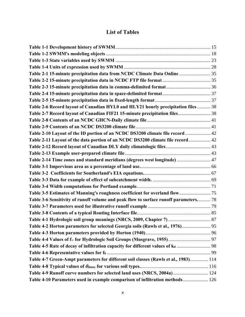
Figure 1-1 Elements of a typical urban drainage system.

• The Atmosphere compartment, which generates precipitation and deposits pollutants onto the Land Surface compartment.

• The Land Surface compartment receives precipitation from the Atmosphere compartment in the form of rain or snow. It sends outflow in the forms of 1) evaporation back to the Atmosphere compartment, 2) infiltration into the Sub-Surface compartment and 3) surface runoff and pollutant loadings on to the Conveyance compartment.

• The Sub-Surface compartment receives infiltration from the Land Surface compartment and transfers a portion of this inflow to the Conveyance compartment as groundwater interflow.

• The Conveyance compartment contains a network of elements (channels, pipes, pumps, and regulators) and storage/treatment units that convey water to outfalls or to treatment facilities. Inflows to this compartment can come from surface runoff, groundwater interflow, sanitary dry weather flow, or from user-defined time series.

Not all compartments need appear in a particular SWMM model. For example, one could model just the Conveyance compartment, using pre-defined hydrographs and pollutographs as inputs. As illustrated in Figure 1-1, SWMM can be used to model any combination of stormwater collection

17

systems, both separate and combined sanitary sewer systems, as well as natural catchment and river channel systems. Figure 1-2 shows how SWMM conceptualizes the physical elements of the actual system depicted in Figure 1-1 with a standard set of modeling objects. The principal objects used to model the rainfall/runoff process are Rain Gages and Subcatchments. Snowmelt is modeled with Snow Pack objects placed on top of subcatchments while Aquifer objects placed below subcatchments are used to model groundwater flow. The conveyance portion of the drainage system is modeled with a network of Nodes and Links. Nodes are points that represent simple junctions, flow dividers, storage units, or outfalls. Links connect nodes to one another with conduits (pipes and channels), pumps, or flow regulators (orifices, weirs, or outlets). Land Use and Pollutant objects are used to describe water quality. Finally, a group of data objects that includes Curves, Time Series, Time Patterns, and Control Rules, are used to characterize the inflows and operating behavior of the various physical objects in a SWMM model. Table 1-2 provides a summary of the various objects used in SWMM. Their properties and functions will be described in more detail throughout the course of this manual.

Figure 1-2 SWMM's conceptual model of a stormwater drainage system.

18

Table 1-2 SWMM's modeling objects

Category Object Type Description

Hydrology Rain Gage Source of precipitation data to one or more subcatchments.

Subcatchment A land parcel that receives precipitation associated with a rain gage and generates runoff that flows into a drainage system node or to another subcatchment.

Aquifer A subsurface area that receives infiltration from the subcatchment above it and exchanges groundwater flow with a conveyance system node.

Snow Pack Accumulated snow that covers a subcatchment.

Unit Hydrograph

A response function that describes the amount of sewer inflow/infiltration generated over time per unit of instantaneous rainfall.

Hydraulics Junction A point in the conveyance system where conduits connect to one another with negligible storage volume (e.g., manholes, pipe fittings, or stream junctions).

Outfall An end point of the conveyance system where water is discharged to a receptor (such as a receiving stream or treatment plant) with known water surface elevation.

Divider A point in the conveyance system where the inflow splits into two outflow conduits according to a known relationship.

Storage Unit A pond, lake, impoundment, or chamber that provides water storage.

Conduit A channel or pipe that conveys water from one conveyance system node to another.

Pump A device that raises the hydraulic head of water.

Regulator A weir, orifice or outlet used to direct and regulate flow between two nodes of the conveyance system.

19

Table 1-2 SWMM’s modeling objects (continued)

Category Object Type Description

Water Quality Pollutant A contaminant that can build up and be washed off of the land surface or be introduced directly into the conveyance system.

Land Use A classification used to characterize the functions that describe pollutant buildup and washoff.

Treatment LID Control A low impact development control, such as a bio-retention cell, porous pavement, or vegetative swale, used to reduce surface runoff through enhanced infiltration.

Treatment Function

A user-defined function that describes how pollutant concentrations are reduced at a conveyance system node as a function of certain variables, such as concentration, flow rate, water depth, etc.

Data Object Curve A tabular function that defines the relationship between two quantities (e.g., flow rate and hydraulic head for a pump, surface area and depth for a storage node, etc.).

Time Series A tabular function that describes how a quantity varies with time (e.g., rainfall, outfall surface elevation, etc.).

Time Pattern A set of factors that repeats over a period of time (e.g., diurnal hourly pattern, weekly daily pattern, etc.).

Control Rules IF-THEN-ELSE statements that determine when specific control actions are taken (e.g., turn a pump on or off when the flow depth at a given node is above or below a certain value).

20

1.3 SWMM’s Process Models Figure 1-3 depicts the processes that SWMM models using the objects described previously and how they are tied to one another. The hydrological processes depicted in this diagram include:

Figure 1-3 Processes modeled by SWMM.

• time-varying precipitation

• snow accumulation and melting

• rainfall interception from depression storage (initial abstraction)

Precipitation

Snowmelt

Evaporation/ Infiltration

Groundwater

Surface Runoff

Channel, Pipe & Storage Routing

Washoff

Sanitary Flows

RDII Treatment / Diversion

Buildup

LID Controls

Initial Abstraction

21

• evaporation of standing surface water

• infiltration of rainfall into unsaturated soil layers

• percolation of infiltrated water into groundwater layers

• interflow between groundwater and the drainage system

• nonlinear reservoir routing of overland flow

• infiltration and evaporation of rainfall/runoff captured by Low Impact Development controls.

The hydraulic processes occurring within SWMM’s conveyance compartment include:

• external inflow of surface runoff, groundwater interflow, rainfall-dependent infiltration/inflow, dry weather sanitary flow, and user-defined inflows

• unsteady, non-uniform flow routing through any configuration of open channels, pipes and storage units

• various possible flow regimes such as backwater, surcharging, reverse flow, and surface ponding

• flow regulation via pumps, weirs, and orifices including time- and state-dependent control rules that govern their operation.

Regarding water quality, the following processes can be modeled for any number of user-defined water quality constituents:

• dry-weather pollutant buildup over different land uses

• pollutant washoff from specific land uses during storm events

• direct contribution of rainfall deposition

• reduction in dry-weather buildup due to street cleaning

• reduction in washoff loads due to BMPs

• entry of dry weather sanitary flows and user-specified external inflows at any point in the drainage system

• routing of water quality constituents through the drainage system

• reduction in constituent concentration through treatment in storage units or by natural processes in pipes and channels.

22

The numerical procedures that SWMM uses to model the hydrologic processes listed above are discussed in detail in subsequent chapters of this volume. SWMM’s hydraulic, water quality, treatment and low impact development processes are described in subsequent volumes of this manual.

1.4 Simulation Process Overview SWMM is a distributed discrete time simulation model. It computes new values of its state variables over a sequence of time steps, where at each time step the system is subjected to a new set of external inputs. As its state variables are updated, other output variables of interest are computed and reported. This process is represented mathematically with the following general set of equations that are solved at each time step as the simulation proceeds:

𝑋𝑋𝑡𝑡 = 𝑓𝑓(𝑋𝑋𝑡𝑡−1, 𝐼𝐼𝑡𝑡, 𝑃𝑃) (1-1)

𝑌𝑌𝑡𝑡 = 𝑔𝑔(𝑋𝑋𝑡𝑡, 𝑃𝑃) (1-2) where

Xt = a vector of state variables at time t, Yt = a vector of output variables at time t, It = a vector of inputs at time t, P = a vector of constant parameters, f = a vector-valued state transition function, g = a vector-valued output transform function.

Figure 1-4 depicts the simulation process in block diagram fashion.

Figure 1-4 Block diagram of SWMM's state transition process.

X0

I1

X1

Y1

Xt--1

It

Xt

Yt

• • •

• • • f(X0, I1, P) f(Xt-1, It, P) g(X1, P) g(Xt, P)

23

The variables that make up the state vector Xt are listed in Table 1-3. This is a surprisingly small number given the comprehensive nature of SWMM. All other quantities can be computed from these variables, external inputs, and fixed input parameters. The meaning of some of the less obvious state variables, such as those used for snow melt, is discussed in later chapters.

Table 1-3 State variables used by SWMM

Process Variable Description Initial Value Runoff d Depth of runoff on a subcatchment surface 0

Infiltration* tp Equivalent time on the Horton curve 0

Fe Cumulative excess infiltration volume 0

Fu Upper zone moisture content 0

T Time until the next rainfall event 0

P Cumulative rainfall for current event 0

S Soil moisture storage capacity remaining User supplied

Groundwater θu Unsaturated zone moisture content User supplied

dL Depth of saturated zone User supplied

Snowmelt wsnow Snow pack depth User supplied

fw Snow pack free water depth User supplied

ati Snow pack surface temperature User supplied

cc Snow pack cold content 0

Flow Routing y Depth of water at a node User supplied

q Flow rate in a link User supplied

a Flow area in a link Inferred from q

Water Quality tsweep Time since a subcatchment was last swept User supplied

mB Mass of pollutant on subcatchment surface User supplied

mP Mass of pollutant ponded on subcatchment 0

cN Concentration of pollutant at a node User supplied

cL Concentration of pollutant in a link User supplied *Only a sub-set of these variables is used, depending on the user’s choice of infiltration method. Examples of user-supplied input variables It that produce changes to these state variables include:

24

• meteorological conditions, such as precipitation, air temperature, potential evaporation rate and wind speed

• externally imposed inflow hydrographs and pollutographs at specific nodes of the conveyance system

• dry weather sanitary inflows to specific nodes of the conveyance system

• water surface elevations at specific outfalls of the conveyance system

• control settings for pumps and regulators. The output vector Yt that SWMM computes from its updated state variables contains such reportable quantities as:

• runoff flow rate and pollutant concentrations from each subcatchment

• snow depth, infiltration rate and evaporation losses from each subcatchment

• groundwater table elevation and lateral groundwater outflow for each subcatchment

• total lateral inflow (from runoff, groundwater flow, dry weather flow, etc.), water depth, and pollutant concentration for each conveyance system node

• overflow rate and ponded volume at each flooded node

• flow rate, velocity, depth and pollutant concentration for each conveyance system link. Regarding the constant parameter vector P, SWMM contains over 150 different user-supplied constants and coefficients within its collection of process models. Most of these are either physical dimensions (e.g., land areas, pipe diameters, invert elevations) or quantities that can be obtained from field observation (e.g., percent impervious cover), laboratory testing (e.g., various soil properties), or previously published data tables (e.g., pipe roughness based on pipe material). A smaller remaining number might require some degree of model calibration to determine their proper values. Not all parameters are required for every project (e.g., the 14 groundwater parameters for each subcatchment are not needed if groundwater is not being modeled). The subsequent chapters of this manual carefully define each parameter and make suggestions on how to estimate its value. A flowchart of the overall simulation process is shown in Figure 1-5. The process begins by reading a description of each object and its parameters from an input file whose format is described in the SWMM 5 UsersManual (US EPA, 2010). Next the values of all state variables are initialized, as is the current simulation time (T), runoff time (Troff), and reporting time (Trpt).

25

Figure 1-5 Flow chart of SWMM's simulation procedure.

Read Input Parameters

Initialize State Variables

T = 0 Troff = 0

Trpt = ∆Trpt

T >= Stop

T1 = T + ∆Trout

Troff < T1 Compute Runoff

Troff = Troff + ∆Troff

Route Flows and Water Quality

Trpt < T1

T = T1

Save Output Results Trpt = Trpt+ ∆Trpt

YES

YES

YES

Legend: T = current elapsed time T1 = new elapsed time Troff = current runoff time Trpt = current reporting time ∆Trout = routing time step ∆Troff = runoff time step ∆Trpt = reporting time step DUR = simulation duration

26

The program then enters a loop that first determines the time T1 at the end of the current routing time step (∆Trout). If the current runoff time Troff is less than T1, then new runoff calculations are repeatedly made and the runoff time updated until it equals or exceeds time T1. Each set of runoff calculations accounts for any precipitation, evaporation, snowmelt, infiltration, ground water seepage, overland flow, and pollutant buildup and washoff that can contribute flow and pollutant loads into the conveyance system. Once the runoff time is current, all inflows and pollutant loads occurring at time T are routed through the conveyance system over the time interval from T to T1. This process updates the flow, depth and velocity in each conduit, the water elevation at each node, the pumping rate for each pump, and the water level and volume in each storage unit. In addition, new values for the concentrations of all pollutants at each node and within each conduit are computed. Next a check is made to see if the current reporting time Trpt falls within the interval from T to T1. If it does, then a new set of output results at time Trpt are interpolated from the results at times T and T1 and are saved to an output file. The reporting time is also advanced by the reporting time step ∆Trpt. The simulation time T is then updated to T1 and the process continues until T reaches the desired total duration. SWMM’s Windows-based user interface provides graphical tools for building the aforementioned input file and for viewing the computed output.

1.5 Interpolation and Units SWMM uses linear interpolation to obtain values for quantities at times that fall in between times at which input time series are recorded or at which output results are computed. The concept is illustrated in Figure 1-6 which shows how reported flow values are derived from the computed flow values on either side of it for the typical case where the reporting time step is larger than the routing time step. One exception to this convention is for precipitation and infiltration rates. These remain constant within a runoff time step and no interpolation is made when these values are used within SWMM’s runoff algorithms or for reporting purposes. In other words, if a reporting time falls within a runoff time step the reported rainfall intensity is the value associated with the start of the runoff time step.

27

Figure 1-6 Interpolation of reported values from computed values.

The units of expression used by SWMM’s input variables, parameters, and output variables depend on the user’s choice of flow units. If flow rate is expressed in US customary units then so are all other quantities; if SI metric units are used for flow rate then all other quantities use SI metric units. Table 1-4 lists the units associated with each of SWMM’s major variables and parameters, for both US and SI systems. Internally within the computer code all calculations are carried out using feet as the unit of length and seconds as the unit of time and then converted back to the user’s choice of unit system.

Time

F L O W

∆Trpt

∆Trout

Computed

Interpolated

28

Table 1-4 Units of expression used by SWMM

Variable or Parameter US Customary Units SI Metric Units

Area (subcatchment) acres hectares

Area (storage surface area) square feet square meters

Depression Storage inches millimeters

Depth feet meters

Elevation feet meters

Evaporation inches/day millimeters/day

Flow Rate cubic feet/sec (cfs) gallons/min (gpm) 106 gallons/day (mgd)

cubic meters/sec (cms) liters/sec (lps) 106 liters/day (mld)

Hydraulic Conductivity inches/hour millimeters/hour

Hydraulic Head feet meters

Infiltration Rate inches/hour millimeters/hour

Length feet meters

Manning’s n seconds/meter1/3 seconds/meter1/3

Pollutant Buildup mass/acre mass/hectare

Pollutant Concentration milligrams/liter (mg/L) micrograms/liter (µg/L) organism counts/liter

milligrams/liter (mg/L) micrograms/liter (µg/L) organism counts/liter

Rainfall Intensity inches/hour millimeters/hour

Rainfall Volume inches millimeters

Storage Volume cubic feet cubic meters

Temperature degrees Fahrenheit degrees Celsius

Velocity feet/second meters/second

Width feet meters

Wind Speed miles/hour kilometers/hour

29

Chapter 2 – Meteorology

2.1 Precipitation

2.1.1 Representation Precipitation is the principal driving force in rainfall-runoff-quality simulation. Stormwater runoff and nonpoint source runoff quality are directly dependent on the precipitation time series. These time series can range from just a few time periods for a single event to thousands of time periods used for a multi-year simulation. Within SWMM, the Rain Gage object is used to represent a source of precipitation data. Any number of Rain Gages may be used, data permitting, to represent spatial variability in precipitation patterns. Precipitation data for a specific Rain Gage is supplied either as a user-defined Time Series or through an external data file. Several different file formats are supported for data distributed by the U.S. National Climatic Data Center and Environment Canada as well as a standard user-prepared format. Because SWMM is a fully dynamic model that accounts for physical processes whose time scales are on the order of minutes or less, SWMM should not be run with either daily average or storm-averaged precipitation data. Note that precipitation is often used synonymously with rainfall, but precipitation data may also include snowfall. Because both are simply reported as incremental intensities or depths, the SWMM program differentiates between rainfall and snowfall by a user-supplied dividing temperature. In natural areas, a surface temperature of 34° to 35° F (1-2° C) provides the dividing line between equal probabilities of rain and snow (Eagleson, 1970; Corps of Engineers, 1956). However, this separation temperature might need to be somewhat lower in urban areas due to warmer surface temperatures.

2.1.2 Single Event v. Continuous Simulation Models might be used to aid in urban drainage design for protection against flooding for a certain return period (e.g., five or ten years), or to protect against pollution of receiving waters at a certain frequency (e.g., only one combined sewer overflow per year). In these contexts, the frequency or return period needs to be associated with a very specific parameter. That is, for rainfall one may speak of frequency distributions of inter-event times, total storm depth, total storm duration or average storm intensity, all of which are different (Eagleson, 1970, pp. 183-190). But for the aforementioned objectives, and in fact, for almost all urban hydrology work, the frequencies of runoff and quality parameters are required, not those of rainfall. Thus, one may speak of the frequencies of maximum flow rate, total runoff volume, or total pollutant loads. These distributions are in no way the same as for similar rainfall parameters, although they may be related

30

through analytical methods (Howard, 1976; Chan and Bras, 1979; Hydroscience, 1979; Adams and Papa, 2000). Finally, for pollution control, the real interest may lie in the frequency of water quality standards violations in the receiving water, which leads to further complications. SWMM is capable of simulating both single rainfall events as well as long-term time histories (e.g. several years or more) of a continuous precipitation record. In fact, the only distinctions between the two as far as SWMM is concerned is the simulation duration requested by the user and the need to supply meaningful initial conditions when only a single event is simulated. Continuous simulation offers an excellent, if not the only method for obtaining the frequency of events of interest, be they related to quantity or quality. But it has the disadvantages of a higher run time and the need for a continuous rainfall record. This has led to the use of a “design storm” or “design rainfall” or “design event” in a single event simulation instead. Of course, this idea long preceded continuous simulation, before the advent of modern computers. However, because of inherent simplifications, the choice of a design event leads to problems.

2.1.3 Temporal Rainfall Variations The required time interval used to describe rainfall variations over time is a function of the catchment response to rainfall input. Small, steep, smooth, impervious catchments have fast response times, while large, flat, pervious catchments have slower response times. As a generality, shorter time increment data are preferable to longer time increment data, but for a large (e.g., 10 mi2 or 26 km2) subcatchment (coarse schematization), even the hourly inputs usually used for continuous simulation may be appropriate. Rainfall data with intervals larger than 1-hour (such as average daily rainfall or event-averaged rainfall) must be suitably disaggregated (Socolofsky et al., 2001) before they can be used in SWMM. The rain gage itself is usually the limiting factor. It is possible to reduce data from 24-hour charts from standard 24-hour, weighing-bucket gages to obtain 7.5-minute or 5-minute increment data, and some USGS float gages produce no better than 5-minute values. Shorter time increment data may usually be obtained only from tipping bucket gage installations. The rainfall records obtained from a gage may be of mixed quality. It may be possible to define some storms down to 1 to 5 minute rainfall intensities, while other events may be of such poor quality (because of poor reproduction of charts or blurred traces of ink) that only 1-hour increments can be obtained.

31

2.1.4 Spatial Rainfall Variations Even for small catchments, runoff and consequent model predictions (and prototype measurements) may be very sensitive to spatial variations of the rainfall. For instance, thunderstorms (convective rainfall) may be highly localized, and nearby gages may have very dissimilar readings. For modeling accuracy (or even more specifically, for a successful calibration of SWMM), it is essential that rain gages be located within and adjacent to the catchment. SWMM accounts for the spatial variability of rainfall by allowing the user to define any number of Rain Gage objects along with their individual data sources, and assign any rain gage to a particular SWMM Subcatchment object (i.e., land parcel) from which runoff is computed. If multiple gages are available, this is a much better procedure than is the use of spatially averaged (e.g., Thiessen weighted) data, because averaged data tend to have short-term time variations removed (i.e., rainfall pulses are “lowered” and “spread out”). In general, if the rainfall is uniform spatially, as might be expected from cyclonic (e.g., frontal) systems, these spatial considerations are not as important. In making this judgment, the storm size and speed in relation to the total study area size must be considered. Storm movement can significantly affect hydrographs computed at the catchment outlet (Yen and Chow, 1968; Surkan, 1974; James and Drake, 1980; James and Shtifter, 1981).When more than one gage is available to apply to the simulation, it is possible to simulate moving storms, as rainfall in one part of the basin may be different from rainfall in another part of the basin. Movement of a storm in the downstream direction increases the hydrograph peak, while movement upstream tends to level out the hydrograph (Surkan, 1974; James and Drake, 1980; James and Shtifter, 1981). For detailed simulation of large cities, radar rainfall data are very useful. Commercial firms specializing in provision of radar rainfall values may be able to place highly spatially and temporally variable rainfall data into a time series format easily input to SWMM (e.g., Hoblit and Curtis, 2002; Meeneghan et al., 2002, 2003; Vallabhaneni, 2002). Radar data are spatially averaged over uniform grid cells of 1 km2 or larger and therefore each cell would cover a number of runoff subcatchments. In this case one could simply use a separate Rain Gage object for each grid cell that overlaps the study area, and assign the nearest cell as the subcatchment’s source of rainfall data. A more sophisticated approach is to define a separate Rain Gage for each subcatchment along with a weighting matrix W whose entries wij represent the fraction of area from subcatchment i that is contained in grid cell j. Then at any time t the vector of subcatchment rainfalls It would equal the vector of cell rainfall values Rt multiplied by the weighting matrix W. These data for each time period could be placed in a standard SWMM user-prepared rainfall file for direct use by SWMM (see below).

32

2.2 Precipitation Data Sources

2.2.1 User-Supplied Data Many SWMM analyses will rely upon rainfall data supplied by the user, on the basis of measurements made at the closest rain gages to the catchment, or on an assumed design storm, either “real” (that is, derived from actual measurements) or “synthetic” (derived from an assumed duration and temporal distribution). Construction of synthetic design storms is described in many texts and manuals, e.g., Chow et al. (1988), King County Department of Public Works (1995), Bedient et al. (2013); SWMM does not supply synthetic design storms automatically, since the emphasis is more properly on use of measured data. Measured data may be from National Weather Service (NWS) or Environment Canada sites, as described below, from local agencies (e.g., utilities), from special monitoring programs (e.g., by the USGS or at a university), or from several other sources, even from home weather stations. Naturally, the quality of any data source should be investigated. User-supplied rainfall data are provided to SWMM using a Rain Gage object. The user specifies the format in which the rainfall data were recorded (as intensity, volume, or cumulative volume), the time interval associated with each rainfall reading (e.g., 15 minutes, 1 hour, etc.), the source of the data (the name of a Time Series object or name of a Rainfall file), and the ID name of the recording station or data source if a file is being used. For rainfall time series, only periods with non-zero precipitation need be included in the series. Using a Time Series object for user-supplied rainfall data makes sense for single-event or short duration simulation periods where there are a limited number of Rain Gage objects. In fact it is possible to create several different time series for a given rain gage in a SWMM project, where each contains a different rainfall event to be analyzed. Then all one needs to do is select the appropriate time series for the scenario of interest. If a Rainfall file is used for user-supplied rainfall data then it must follow SWMM’s standard user-prepared format. Each line of the file contains the station ID, year, month, day, hour, minute, and non-zero precipitation reading, each separated by one or more spaces. There is no need to include time periods with zero readings. An excerpt from a sample user-prepared Rainfall data file might look as follows (i.e., Station STA01 recorded 0.12 inches of rainfall between midnight and one am on June 12, 2004):

33

Using a Rainfall file to provide precipitation data is more convenient when a long-term continuous simulation is being made or when there are many rain gages in a project. Note that it is possible for a single user-prepared Rainfall file to contain data from more than one recording station or external data source as would be the case in the radar data example discussed previously. SWMM’s rainfall Time Series and user-prepared Rainfall files treat the data as “start-of-interval” values, meaning that each rainfall intensity or depth is assumed to occur at the start of its associated date/time value and last for a period of time equal to the gage’s recording interval. Most rainfall recording devices report their readings as “end-of-interval” values, meaning that the time stamp associated with a rainfall value is for the end of the recording interval. If such data are being used to populate a SWMM rainfall time series or user-prepared rainfall file then their date/time values should be shifted back one recording interval to make them represent “start-of-interval” values (e.g., for hourly rainfall, a reading with a time stamp of 10:00 am should be entered into the time series or file as a 9:00 am value).

2.2.2 Data from Government Agencies SWMM can also use rainfall data from files provided directly from US and Canadian government agencies. The National Weather Service (NWS) makes available historical hourly precipitation values (including water equivalent of snowfall depths) for about 5,500 observational stations around the U.S., with the periods of record usually beginning in the late 1940s. Fifteen-minute data are available for over 2,400 stations, with records typically beginning in the early 1970s. The repository for U.S. weather data is the National Oceanic and Atmospheric Administration (NOAA) National Climatic Data Center (NCDC), located in Asheville, North Carolina. Key access information is provided below:

National Climatic Data Center Climate Services Branch 151 Patton Avenue Asheville, NC 28801 Telephone: 828-271-4800 Web: http://www.ncdc.noaa.gov/

STA01 2004 6 12 00 00 0.12 STA01 2004 6 12 01 00 0.04 STA01 2004 6 22 16 00 0.07

34

The NCDC digital data bases that house the precipitation data are designated as DSI-3240 for hourly precipitation and DSI-3260 for 15-minute precipitation. NOAA’s Climate Data Online (CDO) service at http://www.ncdc.noaa.gov/cdo-web provides free access to these archives in addition to station history information. It features an interactive map application that helps locate a recording station closest to a site of interest and allows one to request precipitation data for a stipulated period of record. After a data request has been made through CDO the user receives an email with a link to a web page where the data can be viewed with a web browser. The page can then be saved to file for future use with SWMM. When requesting data from CDO be sure to specify the TEXT format option and not the CSV option so that SWMM can automatically recognize the file format and parse its contents. In addition, select the QPCP precipitation option, not the QGAG option, for 15-minute precipitation and make sure that the data flags are included. Table 2.1 shows 15-minute precipitation data downloaded for station 410427 from Austin, Texas. The column headings represent:

Station: cooperative recording station identifier.

Date: date and time at end of fifteen minute recording period.

QPCP: precipitation amount in hundredths of an inch (where 9999 or 99999 indicates a missing value).

Measurement if present, a flag that denotes either the start or end of an accumulation Flag: period, a deleted period or a missing period.

Quality Flag: if present, a flag that indicates if the data value is erroneous.

Units: a flag indicating the precision of the recorded value where HI is for hundredths and HT for tenths of an inch.

Hourly precipitation has a similar format except that the label ‘HPCP’ (for hourly precipitation) replaces ‘QPCP’ and there is no Units column since the data precision is always HT. These data sets only include periods with non-zero precipitation, use time stamps that mark the end of the recording interval, and use a time of ‘00:00’ to refer to midnight of the previous day. SWMM recognizes these conventions, as well as missing value codes, when it reads a precipitation data file.

35

Table 2-1 15-minute precipitation data from NCDC Climate Data Online

STATION DATE QPCP Measurement Flag Quality Flag Units ----------- -------------- ---------------- ----- ----- ------------COOP:410427 19970729 07:45 10 HT COOP:410427 19970730 16:15 70 HT COOP:410427 19970730 16:30 20 HT COOP:410427 19970730 16:45 30 HT COOP:410427 19970730 17:00 50 HT COOP:410427 19970730 17:15 30 HT COOP:410427 19970730 17:30 10 HT COOP:410427 19970730 18:00 20 HT COOP:410427 19970730 18:15 20 HT COOP:410427 19970730 18:45 10 HT COOP:410427 19970730 19:30 10 HT COOP:410427 19970731 08:30 10 HT

The NOAA-NCDC web site also allows one to access the complete set of hourly and 15-minute precipitation data for a particular station through an FTP server (see http://www.ncdc.noaa.gov/cdo-web/datasets). For each station, there is one file that houses data from 1948 (1971 for 15-minute data) to 1998 and then separate files for each year afterward. Each line in these files contains one day’s worth of precipitation data using the format shown in Table 2.2. Note that the third and fourth lines are “wrapped around” as a continuation of the long second line. These are the same Austin, Texas data listed in Table 2.1 with the addition of an hour ‘2500’ entry on each line that contains the daily total. Also these files use hour ‘2400’ to represent midnight unlike hour ’00:00’ used in the Climate Data Online format.

Table 2-2 15-minute precipitation data in NCDC FTP file format

Earlier online data formats used by NCDC can also be recognized by SWMM. Examples of these formats, for the 15-minute Austin, Texas data, are shown in Tables 2.3 through 2.5. The formats for hourly data are identical, except that HPCP replaces QPCP and time stamps are always for hours only.

15M41042707QPCPHT19970700290020745 00010 2500 00010 15M41042707QPCPHT19970700300111615 00070 1630 00020 1645 00030 1700 00050 1715 00030 1730 00010 1800 00020 1815 00020 1845 00010 1930 00010 2500 00270 15M41042707QPCPHT19970700310020830 00010 2500 00010

36

Long precipitation records are subject to meter malfunctions and missing data (for any reason). The NWS has special codes for its DSI-3240 and DSI-3260 formats denoting these conditions. They are explained in the NCDC documentation for each type. SWMM will note the number of recording periods with missing data, often denoted with a 9999 in the rainfall column. Rainfall time series used by the subcatchment object contain only good, non-zero precipitation data.

Table 2-3 15-minute precipitation data in comma-delimited format

COOPID,CD,ELEM,UN,YEAR,MO,DA,TIME, VALUE,F,F ------,--,----,--,----,--,--,----,------,-,- 410427,07,QPCP,HT,1997,07,29,0745, 00010, , 410427,07,QPCP,HT,1997,07,29,2500, 00010, , 410427,07,QPCP,HT,1997,07,30,1615, 00070, , 410427,07,QPCP,HT,1997,07,30,1630, 00020, , 410427,07,QPCP,HT,1997,07,30,1645, 00030, , 410427,07,QPCP,HT,1997,07,30,1700, 00050, , 410427,07,QPCP,HT,1997,07,30,1715, 00030, , 410427,07,QPCP,HT,1997,07,30,1730, 00010, , 410427,07,QPCP,HT,1997,07,30,1800, 00020, , 410427,07,QPCP,HT,1997,07,30,1815, 00020, , 410427,07,QPCP,HT,1997,07,30,1845, 00010, , 410427,07,QPCP,HT,1997,07,30,1930, 00010, , 410427,07,QPCP,HT,1997,07,30,2500, 00270, , 410427,07,QPCP,HT,1997,07,31,0830, 00010, , 410427,07,QPCP,HT,1997,07,31,2500, 00010, ,

37

Table 2-4 15-minute precipitation data in space-delimited format

COOPID CD ELEM UN YEAR MO DA TIME VALUE F F ------ -- ---- -- ---- -- -- ---- ------ - - 410427 07 QPCP HT 1997 07 29 0745 00010 410427 07 QPCP HT 1997 07 29 2500 00010 410427 07 QPCP HT 1997 07 30 1615 00070 410427 07 QPCP HT 1997 07 30 1630 00020 410427 07 QPCP HT 1997 07 30 1645 00030 410427 07 QPCP HT 1997 07 30 1700 00050 410427 07 QPCP HT 1997 07 30 1715 00030 410427 07 QPCP HT 1997 07 30 1730 00010 410427 07 QPCP HT 1997 07 30 1800 00020 410427 07 QPCP HT 1997 07 30 1815 00020 410427 07 QPCP HT 1997 07 30 1845 00010 410427 07 QPCP HT 1997 07 30 1930 00010 410427 07 QPCP HT 1997 07 30 2500 00270 410427 07 QPCP HT 1997 07 31 0830 00010 410427 07 QPCP HT 1997 07 31 2500 00010

Table 2-5 15-minute precipitation data in fixed-length format

15M41042707QPCPHT19970700290020745 00010 15M41042707QPCPHT19970700290022500 00010 15M41042707QPCPHT19970700300111615 00070 15M41042707QPCPHT19970700300111630 00020 15M41042707QPCPHT19970700300111645 00030 15M41042707QPCPHT19970700300111700 00050 15M41042707QPCPHT19970700300111715 00030 15M41042707QPCPHT19970700300111730 00010 15M41042707QPCPHT19970700300111800 00020 15M41042707QPCPHT19970700300111815 00020 15M41042707QPCPHT19970700300111845 00010 15M41042707QPCPHT19970700300111930 00010 15M41042707QPCPHT19970700300112500 00270 15M41042707QPCPHT19970700310020830 00010 15M41042707QPCPHT19970700310022500 00010

38

SWMM can also automatically recognize and read Canadian precipitation data that are stored in climatologic files available from Environment Canada: (http://www.climate.weather.gc.ca). SWMM accepts hourly data from HLY03 and HLY21 files and 15-minute data from FIF21 files: (http://climate.weather.gc.ca/prods_servs/documentation_index_e.html). Tables 2-6 and 2-7 show the layout of the data records in these files, respectively. The “ELEM” field would contain the code 123 for rainfall, the “S” field is for a numerical sign, the “VALUE” field has units of 0.1 mm, and the “F” and “FLG” fields are for data quality flags. SWMM makes the proper adjustment from “end-of-interval” to “start-of-interval” when processing the Canadian precipitation files. As of this writing, these files are only available through custom requests made to Environment Canada for a fee.

Table 2-6 Record layout of Canadian HYL0 and HLY21 hourly precipitation files

Table 2-7 Record layout of Canadian FIF21 15-minute precipitation files

When a SWMM rain gage object utilizes any of the standard NCDC or Canadian formatted files, the only information required from the user is the name of file that contains the data and a station ID. The latter need not be the same as the station ID referenced in the file. Other user-editable rain gage properties, such as data format, interval, and units are overridden by the values associated with the particular data file. SWMM will also convert the depth units used in the file to the user’s choice of unit system. For example, if an NCDC fifteen-minute rainfall file is used in a SWMM project that employs SI metric units then SWMM knows that the file’s data must first be converted from tenths of an inch per fifteen minute period to mm/hr before they are used for any runoff calculations.

Daily Record of Hourly Data (HLY) - Length 186

| STN ID | YEAR |MO |DY |ELEM |S| VALUE |F| |_|_|_|_|_|_|_|_|_|_|_|_|_|_|_|_|_|_|_|_|_|_|_|_|_|

These fields are repeated 24 times.

Daily Record of 15 Minute Data (FIF) - Length 691

| STN ID | YEAR |MO |DY |ELEM |S| VALUE |F| |FLG| |_|_|_|_|_|_|_|_|_|_|_|_|_|_|_|_|_|_|_|_|_|_|_|_|_| |___|

These fields are repeated 96 times.

39

2.2.3 Rainfall Interface File When precipitation data are supplied to SWMM from one or more external data files, the program first collates the data from these files into a single binary formatted Rainfall Interface file. It is this file that is accessed during the time steps of a SWMM simulation rather than the original rainfall data files. The Rainfall Interface file can be saved to disk and re-used in subsequent runs should the user care to do so. The layout of the interface file is as follows:

The date/time value used here represents the number of decimal days from midnight of December 31, 1899 (i.e., the start of year 1900) expressed as a double precision floating point number. This is the same representation that SWMM uses internally for all date/time values.

2.3 Temperature Data SWMM requires representative air temperature data when simulating snow melt or when using the Hargreaves method to compute potential evapotranspiration. A single set of time-dependent temperatures is applied throughout the study area. These data can come either from a user-generated time series or from a climate file. If a time series is used, then linear interpolation is used to obtain temperature values for times that fall in between those recorded in the time series. The first recorded temperature in the series is used for dates prior to the beginning date of the series while the last recorded temperature is used for dates beyond the end of the series. Temperatures should be in degrees F for SWMM projects built in US units or in degrees C for projects built in metric units.

File stamp ("SWMM5-RAIN") (10 bytes) Number of SWMM rain gages in file (4-byte integer) For each rain gage:

recording station ID (80 bytes) gage recording interval (seconds) (4-byte integer) starting byte of rainfall data in file (4-byte integer) ending byte+1 of rainfall data in file (4-byte integer)

For each rain gage: For each time period with non-zero rainfall:

date/time for start of period (8-byte double) rain depth (inches) (4-byte float)

40

A SWMM climate file contains values for minimum and maximum daily temperatures, (and optionally, evaporation and wind speed). Three climate file formats are supported:

• the current NCDC GHCN-Daily Climate Data Online format • the older NCDC DS3200 (aka TD-3200) format, • Environment Canada’s DLY daily climatologic file format, and • a standard user-prepared format.

The National Climatic Data Center’s Global Historical Climatology Network - Daily (GHCN-Daily) dataset integrates daily climate observations from approximately 30 different data sources for about 30,000 stations across the globe. As with precipitation data, NOAA’s Climate Data Online (CDO) service (http://www.ncdc.noaa.gov/cdo-web) provides free access to these archives. When making an online request for data to be used with SWMM users should do the following:

• select the “Daily Summaries” dataset • select a range of dates to retrieve data from • use the interactive search feature to identify the recording station of interest • select the “Custom GHCN-Daily Text” output format • do not select any of the Station Detail and Data Flag options • select the maximum (TMAX) and minimum (TMIN) air temperature data types • select the average daily wind speed (AWND) and pan evaporation rate (EVAP) data types

if available and if so desired. Some stations will offer 24-hour wind movement (WDMV) instead of average daily wind speed which can be also be selected. Table 2-8 shows the format of the data retrieved for Austin, Texas using the steps listed above. Note that the pan evaporation has units of tenths of millimeters, temperatures are in tenths of a degree Celsius, and 24-hour wind movement is in kilometers. (Had average daily wind speed (AWND) been available it would have units of tenths of meters per second). Data fields with all 9’s in them indicate missing values. SWMM automatically makes the necessary unit conversions when reading this type of climate file. The DS3200 (aka TD-3200) dataset was a predecessor to the GHCN that was discontinued in 2011. SWMM is able to read data files in this older format, an example of which is shown in Table 2-9 for June 1997 for Austin, Texas. Each line of the file begins with “DLY” and contains daily data for an entire month for a specific variable; hence the lines in the table are displayed in wrap around fashion. Table 2-10 describes the format of the ID portion of each record while Table 2-11 does the same for the data portion of the record.

41

Table 2-8 Contents of an NCDC GHCN-Daily climate file

Table 2-9 Contents of an NCDC DS3200 climate file

STATION DATE EVAP TMAX TMIN WDMV ----------------- -------- -------- -------- -------- -------- GHCND:USC00410427 19970706 13 350 228 0.7 GHCND:USC00410427 19970707 15 356 233 0.8 GHCND:USC00410427 19970708 10 344 239 1.0 GHCND:USC00410427 19970709 18 356 217 2.5 GHCND:USC00410427 19970710 61 361 222 1.9 GHCND:USC00410427 19970711 30 356 222 1.0 GHCND:USC00410427 19970712 41 356 222 0.8

DLY41042707EVAPHI19970699990060319 00004 00419 00043 00519 00000 00619 00036 01919 00075 03019 00018 0 DLY41042707TMAX F19970699990300119 00086 00219 00091 00319 00091 00419 00091 00519 00089 00619 00088 00719 00083 00819 00087 00919 00088 01019 00087 01119 00090 01219 00091 01319 00092 01419 00093 01519 00094 01619 00092 01719 00093 01819 00094)N1919 00095 02019 00092 02119 00089 02219 00085 02319 00090 02419 00090 02519 00093 02619 00092 02719 00092 02819 00094 02919 00093 03019 00096 0 DLY41042707TMIN F19970699990330119 00067 00219 00055 00319 00062 00419 00063 00519 00069 00619 00068 00719 00063 00819 00067 00919 00066 01019 00068 01119 00069 01219 00072 01319 00079 01419 00077 01519 00076 01619 00074 01719 00075 01819 00070)N1919 00074 02019 00073 02119 00069 02219 00067 02319 00085 22319 00077)S2419 00082 22419 00073 S2519 00089 22519 00069)N2619 00067 02719 00072 02819 00073 02919 00080 03019 00077 0 DLY41042707WDMV M19970699990300119 00027 00219 00025 00319 00017 00419 00016 00519 00022 00619 00022 00719 00018 00819 00016 00919 00020 01019 00050 01119 00022 01219 00018 01319 00053 01419 00039 01519 00037 01619 00005 01719 00051 01819 00079 01919 99999SS2019 00065A02119 00045 02219 00036 02319 00072 02419 00027 02519 00013 02619 00025 02719 00022 02819 00045 02919 00015 03019 00037 0

42

Table 2-10 Layout of the ID portion of an NCDC DS3200 climate file record

Field Width Record Type (always = DLY) 3

Station ID 8

Element Type. Possible types used by SWMM are: TMAX = daily maximum temperature, deg. F TMIN = daily minimum temperature, deg. F EVAP = daily evaporation, in or 1/100 in WDMV = daily wind movement, miles

4

Element Measurement Units Code 2

Year 4

Month 2

Filler (= 9999) 4

Number of data portions that follow 3

Table 2-11 Layout of the data portion of an NCDC DS3200 climate file record (Repeated as many times as needed to contain one month of data).

Field Width Day of Month 2

Hour of Observation 2

Sign of Measured Value 1

Measured Value 5

Quality Control Flag 1 1

Quality Control Flag 2 1

The record layout of the Canadian DLY daily climatologic files is depicted in Table 2-12. The “ELEM” field contains 001 for daily maximum temperature and 002 for daily minimum temperature, the “S” field is for a numerical sign, the “VALUE” field has units of 0.1 deg C, and the “F” field is for a data quality flag. Note that only a single temperature file is used containing records for both daily maximum and daily minimum temperatures. More information on how to obtain these files from Environment Canada can be found at http://www.climate.weather.gc.ca.

43

Table 2-12 Record layout of Canadian DLY daily climatologic files

A user-prepared climate file is a plain text file where each line contains the following items, each separated by one or more spaces:

• recording station name (no spaces allowed) • 4-digit year, • 2-digit month (Jan =1, Feb = 2, etc), • day of the month, • maximum temperature (deg F or C ), • minimum temperature (deg F or C), • evaporation rate (optional, in/day or mm/day), • wind speed (optional, miles/hr or km/hr).

The units used for the various data items must be compatible with the unit system being used in the SWMM project. For temperatures, this means degrees F for US units or degrees C for metric units. If no data are available for a given item on a particular date, then an asterisk should be entered as its value. Table 2-13 is an example of how the contents of the GHCN-Daily file of Table 2-1 would look in user-prepared format under US units.

Table 2-13 Example user-prepared climate file

410427 1997 07 06 95.0 73.0 0.051 0.7 410427 1997 07 07 96.1 73.9 0.059 0.8 410427 1997 07 08 93.9 75.0 0.039 1.0 410427 1997 07 09 96.1 71.1 0.071 2.5 410427 1997 07 10 97.0 72.0 0.240 1.9 410427 1997 07 11 96.1 72.0 0.118 1.0 410427 1997 07 12 96.1 72.0 0.161 0.8

Whenever a climate file is used in SWMM the user can specify a date, different from the simulation starting date, where the program begins reading from. From this date on the daily values are read from the file sequentially, without regard for what date the simulation clock is actually at. This

Monthly Record of Daily Data (DLY) - Length 233

| STN ID | YEAR |MO |ELEM |S| VALUE |F| |_|_|_|_|_|_|_|_|_|_|_|_|_|_|_|_|_|_|_|_|_|_|_|

These two fields are repeated 31 times.

44

feature is useful if one wants to use a rainfall file that covers one span of years and a climate file that covers another. An error message is issued and the program terminates if this starting date does not fall within the dates contained in the file. The same holds true if no file start date was supplied and the simulation start date does not fall within the dates contained in the climate file. When the simulation reaches a date that falls outside the last date in the file, then he program will keep using the temperature values that were last read from the file. The same convention applies whenever there is a gap of missing days or missing data in the file.

2.4 Continuous Temperature Records When temperature data come from a climate file, a mechanism is needed to convert the daily max-min readings into instantaneous values at any point in time during the day. To do this, the minimum temperature is assumed to occur at sunrise each day, and the maximum is assumed to occur three hours prior to sunset. This scheme obviously cannot account for many meteorological phenomena that would create other temperature-time distributions but is apparently an appropriate one under the circumstances. Given the max-min temperatures and their assumed hours of occurrence, temperatures at any other time between these are found by sinusoidal interpolation, as sketched in Figure 2-2. The interpolation is performed, using three different periods: 1) between the maximum of the previous day and the minimum of the present, 2) between the minimum and maximum of the present, and 3) between the maximum of the present and minimum of the following day.

Figure 2-1 Sinusoidal interpolation of hourly temperatures.

45

The time of day of sunrise and sunset are easily obtained as a function of latitude and longitude of the catchment and the date. Techniques for these computations are explained, for example, by List (1966) and by the TVA (1972). Approximate (but sufficiently accurate) formulas used in SWMM are given in the latter reference. (Snowmelt computations that utilize temperatures are generally insensitive to these effects in SWMM.) Their use is explained briefly below.

The hour angle of the sun, h, is the angular distance between the instantaneous meridian of the sun (i.e., the meridian through which passes a line from the center of the earth to the sun) and the meridian of the observer (i.e., the meridian of the catchment). It may be measured in degrees or radians or readily converted to hours, since 24 hours is equivalent to 360 degrees or 2 π radians. The hour angle is a function of latitude, declination of the earth, and time of day and is zero at noon, true solar time, and positive in the afternoon. However, at sunrise and sunset, the solar altitude of the sun (vertical angle of the sun measured from the earth’s surface) is zero, and the hour angle is computed only as a function of latitude and declination,

cos h = - tan δ · tan φ (2-1) where

h = hour angle at sunrise or sunset, radians, δ = earth’s declination, a function of season (date), radians, and φ = latitude of observer, radians.

The earth’s declination is provided in tables (e.g., List, 1966), but for programming purposes an approximate formula is used (TVA, 1972):

𝛿𝛿 = �23.45 𝜋𝜋

180� 𝑐𝑐𝑐𝑐𝑐𝑐 �

2𝜋𝜋365

(172 − 𝐷𝐷)� (2-2)

where D is number of the day of the year (no leap year correction is warranted) and δ is in radians. Having the latitude as an input parameter, the hour angle is thus computed in hours, positive for sunset, negative for sunrise, as

ℎ = (12 𝜋𝜋)𝑐𝑐𝑐𝑐𝑐𝑐−1(− tan 𝛿𝛿 ∙ tan 𝜑𝜑⁄ ) (2-3)

The computation is valid for any latitude between the Arctic and Antarctic Circles, and no correction is made for obstruction of the horizon.

The hour of sunrise and sunset is symmetric about noon, true solar time. True solar noon occurs when the sun is at its highest elevation for the day. It differs from standard zone time, i.e., the time on clocks) because of a longitude effect and because of the “equation of time”. The latter is of

46

astronomical origin and causes a correction that varies seasonally between approximately ± 15 minutes; it is neglected here. The longitude correction accounts for the time difference due to the separation of the meridian of the observer and the meridian of the standard time zone. These are listed in Table 2-14. Note that time zone boundaries are very irregular and often are quite displaced from what might be expected on the basis of the local longitude, e.g., most of Alaska is much further west than the standard meridian for Alaska time of 135oW. The longitude correction is readily computed as

∆𝑇𝑇𝐿𝐿𝐿𝐿𝐿𝐿𝐿𝐿 = 4𝑚𝑚𝑚𝑚𝑚𝑚𝑚𝑚𝑚𝑚𝑚𝑚𝑐𝑐𝑑𝑑𝑚𝑚𝑔𝑔𝑑𝑑𝑚𝑚𝑚𝑚

(𝜃𝜃 − 𝑆𝑆𝑆𝑆) (2-4)

where ∆TLONG = longitude correction, minutes (of time), θ = longitude of the observer, degrees, and SM = standard meridian of the time zone, degrees, from Table 2-14. Note that ∆TLONG can be either positive or negative, and the sign should be retained. For instance, Boston at approximately 71°W has ∆TLONG = -16 minutes, meaning that mean solar noon precedes EST noon by 16 minutes. (Mean solar time differs from true solar time by the neglected “equation of time.”)

The time of day of sunrise is then

𝐻𝐻𝑆𝑆𝑆𝑆 = 12 − ℎ + ∆𝑇𝑇𝐿𝐿𝐿𝐿𝐿𝐿𝐿𝐿/60 (2-5) and the time of day of sunset is

𝐻𝐻𝑆𝑆𝑆𝑆 = 12 + ℎ + ∆𝑇𝑇𝐿𝐿𝐿𝐿𝐿𝐿𝐿𝐿/60 (2-6) From these times, the hours at which the minimum (Tmin) and maximum (Tmax) temperatures occur are Hmin = HSR and Hmax = HSS – 3, respectively.

47

Table 2-14 Time zones and standard meridians (degrees west longitude)

Time Zone Example Cities Standard Meridian

Newfoundland Std. Time St. Johns’s, Newfoundland 52.5a

Atlantic Std. Time Halifax, Nova Scotia San Juan, Puerto Rico

60

Eastern Std. Time New York, New York Toronto, Ontario

75

Central Std. Time Chicago, Illinois Winnipeg, Manitoba Saskatoon, Saskatchewanb

90

Mountain Std. Time Denver, Colorado Edmonton, Alberta

105

Pacific Std. Time San Francisco, California Vancouver, British Columbia Whitehorse, Yukon

120

Alaska Std. Time Anchorage, Alaska 135

Aleutian Std. Time Hawaiian Std. Time

Atka, Alaska Honolulu, Hawaii

150

aThe time zone of the island of Newfoundland is offset one half hour from other zones. bSaskatchewan summer time is Mountain, winter is Central.

The temperature T at any hour H of the day can now be computed as follows:

1. If H < Hmin then

𝑇𝑇 = 𝑇𝑇𝑚𝑚𝑚𝑚𝑚𝑚 +∆𝑇𝑇1

2 𝑐𝑐𝑚𝑚𝑚𝑚 �

𝜋𝜋(𝐻𝐻𝑚𝑚𝑚𝑚𝑚𝑚 − 𝐻𝐻)𝐻𝐻𝑚𝑚𝑚𝑚𝑚𝑚 + 24 − 𝐻𝐻𝑚𝑚𝑚𝑚𝑚𝑚

� (2-7)

where ∆T1 is the difference between the previous day’s maximum temperature and the current day’s minimum temperature.

2. If Hmin ≤ H ≤ Hmax then

48

𝑇𝑇 = 𝑇𝑇𝑚𝑚𝑎𝑎𝑎𝑎 +∆𝑇𝑇2

𝑐𝑐𝑚𝑚𝑚𝑚 �𝜋𝜋�𝐻𝐻𝑚𝑚𝑎𝑎𝑎𝑎 − 𝐻𝐻�𝐻𝐻𝑚𝑚𝑚𝑚𝑚𝑚 − 𝐻𝐻𝑚𝑚𝑚𝑚𝑚𝑚

� (2-8)

where Tavg is the average of Tmin and Tmax, ∆T is the difference between Tmax and Tmin, and Havg is the average of Hmin and Hmax.

3. If H > Hmax then

𝑇𝑇 = 𝑇𝑇𝑚𝑚𝑚𝑚𝑚𝑚 −∆𝑇𝑇2

𝑐𝑐𝑚𝑚𝑚𝑚 �𝜋𝜋(𝐻𝐻 − 𝐻𝐻𝑚𝑚𝑚𝑚𝑚𝑚)

𝐻𝐻𝑚𝑚𝑚𝑚𝑚𝑚 + 24 − 𝐻𝐻𝑚𝑚𝑚𝑚𝑚𝑚� (2-9)

2.5 Evaporation Data Evaporation can occur in SWMM for standing water on subcatchment surfaces, for subsurface water in groundwater aquifers, for water flowing in open channels, for water held in storage units, and for water held in low impact development controls (e.g., green roofs, rain gardens, etc.). Single event simulations are usually insensitive to the evaporation rate, but evaporation can make up a significant component of the water budget during continuous simulation. SWMM allows evaporation rates to be stated as:

• a single constant value,

• a set of monthly average values,

• a user-defined time series of daily values,

• daily values read from an external climate file,

• daily values computed from the daily temperatures in an external climate file. Monthly and seasonal averages for evaporation are available in NOAA (1974) and Farnsworth and Thompson (1982). Another source of evaporation and evapotranspiration data in the U.S. is the AgriMet program of the U.S. Bureau of Reclamation: (http://www.usbr.gov/pn/agrimet/proginfo.html). However, AgriMet is aimed primarily at agricultural use, containing information on crop water use requirements, for instance. Generally, local evaporation data are difficult to obtain. Fortunately, totals are likely to represent large spatial areas more so than for precipitation. State climate agencies are often useful when searching for weather data. For instance, the Oregon

49

Climate Service (http://www.ocs.orst.edu) includes daily pan evaporation data among its weather archives, and links are provided to other climate agencies regionally and nationwide. The climate file source of evaporation data is the same climate file used to supply daily max-min temperatures that was described in section 2.3. For NCDC GHCN-Daily files one would request that records for the element EVAP be included in the file while for the Canadian DLY files one would do the same for daily pan evaporation (element code 151). For the user-supplied climate file, one simply adds an evaporation rate value after the daily minimum temperature entry in each record. If the file were only being used to supply evaporation and not temperatures one still has to enter asterisks (*) in the max and min temperature fields so that the file is read correctly. Note that both the NCDC and Canadian DLY files report pan evaporation while SWMM expects actual evaporation. SWMM will accept a set of monthly pan coefficients, typically on the order of 0.7, used to convert pan evaporation to actual evaporation (Chow et al., 1988; Bedient et al., 2013). Also SWMM will automatically convert the units used for evaporation in these files into the ft/sec units used internally by SWMM. For all other data sources, the evaporation rate values must be in the same unit system as the rest of the data in a project. For US standard units this is inches/day while for SI metric units it is mm/day. SWMM can also use the Hargreaves method (Hargreaves and Samani, 1985) to compute evaporation rates from the daily max-min temperatures contained in a climate file and the study area’s latitude. The governing equation is:

𝐸𝐸 = 0.0023(𝑅𝑅𝑚𝑚 𝜆𝜆⁄ )𝑇𝑇𝑟𝑟1/2(𝑇𝑇𝑚𝑚 + 17.8) (2-10)

where:

E = evaporation rate (mm/day) Ra = water equivalent of incoming extraterrestrial radiation (MJm-2d-1) Tr = average daily temperature range for a period of days (deg C) Ta = average daily temperature for a period of days (deg C) λ = latent heat of vaporization (MJkg-1) = 2.50 – 0.002361Ta

As noted in Hargreaves and Merkley (1998), for the equation to provide satisfactory results Tr and Ta must be averaged over a period of 5 or more days. SWMM therefore uses a 7-day running average of these variables derived from the record of daily max-min temperatures. The extraterrestrial radiation Ra is computed as:

50

Ra = 37.6dr(wssin(φ) sin(δ) + cos(φ) cos(δ) sin(ws)) (2-11) where:

dr = relative earth-sun distance = 1 + 0.033𝑐𝑐𝑐𝑐𝑐𝑐 �

2𝜋𝜋𝜋𝜋365

�

J = Julian day (1 to 365) ws = sunset hour angle (radians) = 𝑐𝑐𝑐𝑐𝑐𝑐−1(− tan 𝜑𝜑 tan 𝛿𝛿) φ = latitude (radians) δ = solar declination (radians) = 0.4093𝑐𝑐𝑚𝑚𝑚𝑚 �

2𝜋𝜋(284 + 𝜋𝜋)365

�

2.6 Wind Speed Data SWMM uses wind speed to refine the calculation of a melting rate for accumulated snow during times when there is precipitation in the form of rainfall (see Section 6.3.2). There are two options for providing wind speed data to SWMM:

• as an average value for each month of the year (January – December)

• from the same climate file used to supply daily max-min temperature and evaporation. For the first option the same monthly average applies no matter which year is being simulated. The wind speed units are miles/hour for US units or km/hour for metric units. The default monthly values are all 0. The NCDC has compiled average monthly wind speeds for various locations throughout the US which can be found at: http://www.ncdc.noaa.gov/sites/default/files/attachments/wind1996.pdf. For the NCDC GHCN-Daily climate file, one can request that records for the average daily wind speed data element AWND or the 24-hour wind movement data element WDMV, whichever is available, be included in the file. For the user-supplied file, wind speed is added after the field for evaporation in each daily record (remember to place a * in the evaporation field if evaporation data is being supplied from some other source). SWMM automatically converts the units used for wind speed by the NCDC file, but for the user-supplied file they must be in miles/hour for US unit system data sets or in km/hour for metric data sets. The Canadian DLY file does not report daily wind speed.

51

Chapter 3 – Surface Runoff

3.1 Introduction This chapter describes how SWMM converts precipitation excess (rainfall and/or snowmelt less infiltration, evaporation, and initial abstraction) into surface runoff (overland flow). Because SWMM is a distributed model it allows a study area to be subdivided into any number of irregularly shaped subcatchment areas to best capture the effect that spatial variability in topography, drainage pathways, land cover, and soil characteristics have on runoff generation. Generation of runoff is therefore computed on a subcatchment by subcatchment basis. SWMM uses a nonlinear reservoir model to estimate surface runoff produced by rainfall over a subcatchment. The model was first published by Chen and Shubinski (1971) and included in the original release of SWMM (Metcalf and Eddy et al., 1971a). Discussions of ancillary processes that serve as components of the runoff model, such as infiltration and snowmelt, are covered elsewhere in this manual.

3.2 Governing Equations SWMM conceptualizes a subcatchment as a rectangular surface that has a uniform slope S and a width W that drains to a single outlet channel as shown in Figure 3-1. Overland flow is generated by modeling the subcatchment as a nonlinear reservoir, as sketched in Figure 3-2.

Figure 3-1 Idealized representation of a subcatchment.

52

Figure 3-2 Nonlinear reservoir model of a subcatchment.

In this representation, the subcatchment experiences inflow from precipitation (rainfall and snowmelt) and losses from evaporation and infiltration. The net excess ponds atop the subcatchment surface to a depth d. Ponded water above the depression storage depth ds can become runoff outflow q. Depression storage accounts for initial rainfall abstractions such as surface ponding, interception by flat roofs and vegetation, and surface wetting. From conservation of mass, the net change in depth d per unit of time t is simply the difference between inflow and outflow rates over the subcatchment:

𝜕𝜕𝑑𝑑𝜕𝜕𝑚𝑚

= 𝑚𝑚 − 𝑚𝑚 − 𝑓𝑓 − 𝑞𝑞 (3-1)

where:

i = rate of rainfall + snowmelt (ft/s) e = surface evaporation rate (ft/s) f = infiltration rate (ft/s) q = runoff rate (ft/s).

Note that the fluxes i, e, f, and q are expressed as flow rates per unit area (cfs/ft2 = ft/s). Assuming that flow across the subcatchment’s surface behaves as if it were uniform flow within a rectangular channel of width W (ft), height d–ds, and slope S, the Manning equation can be used to express the runoff’s volumetric flow rate Q (cfs) as:

d

ds

Runoff

Infiltration

Evaporation Precipitation

53

𝑄𝑄 =1.49

𝑚𝑚𝑆𝑆1/2𝑅𝑅𝑋𝑋

2/3𝐴𝐴𝑋𝑋 (3-2)

Here n is a surface roughness coefficient, S the apparent or average slope of the subcatchment (ft/ft), Ax the area across the subcatchment’s width through which the runoff flows (ft2), and Rx is the hydraulic radius associated with this area (ft). Referring to Figures 3-1 and 3-2, Ax is a rectangular area with width W and height d-ds. Because W will always be much larger than d it follows that 𝐴𝐴𝑋𝑋 = 𝑊𝑊(𝑑𝑑 − 𝑑𝑑𝑆𝑆) and 𝑅𝑅𝑋𝑋 = 𝑑𝑑 − 𝑑𝑑𝑆𝑆. Substituting these expressions into Equation 3-2 gives:

𝑄𝑄 =1.49

𝑚𝑚𝑊𝑊𝑆𝑆1/2(𝑑𝑑 − 𝑑𝑑𝑆𝑆)5/3 (3-3)

To obtain a runoff flow rate per unit of surface area, q, Equation 3-3 is divided by the surface area of the subcatchment, A (which should not be confused with the cross-section area Ax through which the runoff passes):

𝑞𝑞 =1.49𝑊𝑊𝑆𝑆1/2

𝐴𝐴 𝑚𝑚(𝑑𝑑 − 𝑑𝑑𝑆𝑆)5/3 (3-4)

Substituting this equation into the original mass balance relation 3-1 results in:

𝜕𝜕𝑑𝑑𝜕𝜕𝑚𝑚

= 𝑚𝑚 − 𝑚𝑚 − 𝑓𝑓 − 𝛼𝛼(𝑑𝑑 − 𝑑𝑑𝑆𝑆)5/3 (3-5)

where α is defined as:

𝛼𝛼 =1.49𝑊𝑊𝑆𝑆1/2

𝐴𝐴 𝑚𝑚 (3-6)

Equation 3-5 is an ordinary nonlinear differential equation. For known values of i, e, f, ds and α it can be solved numerically over each time step for ponded depth d. Once d is known, values of the runoff rate q can be found from Equation 3-4. Note that Equation 3-5 only applies when d is greater than ds. When d <= ds, runoff q is zero and the mass balance on d becomes simply:

𝜕𝜕𝑑𝑑𝜕𝜕𝑚𝑚

= 𝑚𝑚 − 𝑚𝑚 − 𝑓𝑓 (3-7)

54

3.3 Subcatchment Partitioning The equation used to generate surface runoff was developed on the basis of an idealized rectangular subcatchment area with uniform properties. Urban areas usually contain a mix of land surface types which can conveniently be divided into two primary categories: pervious surfaces (e.g., lawns, fields, and forested areas) which allow rainfall to infiltrate into the soil and impervious surfaces (e.g., roofs, roads, and parking lots) over which no infiltration occurs. Therefore SWMM allows each subcatchment to have both a pervious and impervious subarea over which Equation 3-5 is solved. The user-supplied parameter Percent Imperviousness determines how much of the total subcatchment is devoted to each type of surface. In addition, it is not uncommon for impervious surfaces to begin generating runoff almost immediately after a rainfall event occurs, well before its depression storage depth fills up. To model this behavior, SWMM allows the impervious area of a subcatchment to be further divided into two subareas: one with depression storage and one without. The input parameter % Zero-Imperv determines what fraction of a subcatchment’s impervious area has no depression storage. Thus overall, a subcatchment can contain three types of subareas as shown in Figure 3-3. Note that under these definitions all impervious area is directly connected to the subcatchment’s outlet point (typically a drainage pipe or channel). How to model indirectly connected areas, such as roof drains that discharge to pervious lawn areas, is discussed in section 3.6 below.

Figure 3-3 Types of subareas within a subcatchment.

Conceptually, these three sub-areas are incorporated into the idealized subcatchment as shown in Figure 3-4. Of course in reality the areas will not align in this fashion nor will they necessarily be compact and connected. The arrangement used here is merely a modeling convenience. Symbols A1, A2, and A3 refer to the pervious subarea and two types of impervious subareas (with and without depression storage), respectively, and they discharge their runoff independently of one another to the same outlet location.

55

Figure 3-4 Idealized subcatchment partitioning for overland flow.

With this refinement the governing differential equation 3-5 for subcatchment runoff is solved individually for each subarea. Thus a separate accounting of the ponded depth d over each subarea is maintained. At the end of each time step, the runoff flows from each subarea are combined together to determine a total runoff flow for the entire subcatchment. The following conventions apply when solving the runoff equation for each subarea individually:

• The same precipitation and evaporation rate applies to each subarea.

• The contribution from snowmelt will vary by subarea. See Chapter 6 for details.

• The infiltration rate f is always zero for the two impervious subareas.

• Different values of depression storage ds can be assigned to the pervious (A1) and impervious area (A2), where by definition ds is zero for the impervious area with no depression storage (A3).

• Different values of the Manning roughness n can be used for the pervious (A1) and impervious areas (A2 and A3).

• The same values of W and S apply for all subareas.

A1

A2

A3

A1: pervious area A2: impervious area

w/depression storage A3: impervious area w/o depression storage

To inlet node of pipe or channel

Width

56

The applicable α-terms to be used in Equation 3-5 for each subarea are:

𝛼𝛼𝑃𝑃 =1.49𝑊𝑊𝑆𝑆1/2

𝐴𝐴1𝑚𝑚𝑃𝑃 for the pervious subarea A1 (3-8)

𝛼𝛼𝑃𝑃 =1.49𝑊𝑊𝑆𝑆1/2

(𝐴𝐴2 + 𝐴𝐴3)𝑚𝑚𝐼𝐼 for both impervious subareas A2 and A3 (3-9)

where nP is the roughness for the pervious area, nI is the roughness for both impervious areas, and Ai is the surface area (ft2) associated with sub-area i. The reason that the same α applies to both impervious subareas even though their areas are different arises from how the W/A term is evaluated for the idealized arrangement shown in Figure 3-4. For area A2, W2 = A2W / (A2 + A3) so that W2 / A2 = W / (A2 + A3). For A3, W3 = A3W / (A2 + A3) which results in W3 / A3 = W / (A2 + A3). Thus both types of impervious areas use the same factor W / (A2 + A3).

3.4 Computational Scheme The detailed computational scheme for computing the runoff generated from each subcatchment within a study area over a single time step of a simulation is presented in the sidebar below.

57

Computational Scheme for Runoff

1. If currently there is no precipitation, no snowmelt, and no runoff occurring within the entire study area then set the current time step ∆t equal to the user-specified dry time step. Otherwise set it to the user-specified wet time step. If necessary, reduce the time step to the next time at which either rainfall or evaporation changes. Guidance on time step selection is provided in section 3.5.

2. For each subcatchment, retrieve its current precipitation rate i and evaporation rate e from the data sources described in Chapter 2.

3. For each subarea within each subcatchment:

a. If snow melt is being simulated, use the procedures described in Chapter 6 to adjust the precipitation rate i to reflect any snow accumulation (which decreases i) or snow melt (which increases i).

b. Set the available moisture volume da to 𝑚𝑚∆𝑚𝑚 + 𝑑𝑑 where d is the current ponded depth and limit the evaporation rate e to be no greater than d/∆t.

c. If the subarea is pervious, then determine the infiltration rate f using the methods described in Chapter 4 and if groundwater is being simulated consider the possible reduction in f that can occur due to fully saturated conditions (see Chapter 5). Otherwise set f = 0.

d. If losses exceed the available moisture volume (i.e.,(𝑚𝑚 + 𝑓𝑓)∆𝑚𝑚 ≥ 𝑑𝑑𝑚𝑚) then d = 0 and the runoff rate q is 0. Otherwise, compute the rainfall excess ix as:

𝑚𝑚𝑋𝑋 = 𝑚𝑚 − 𝑚𝑚 − 𝑓𝑓.

e. If the rainfall excess is not enough to fill the depression storage depth ds over the time step (i.e.,𝑑𝑑 + 𝑚𝑚𝑋𝑋∆𝑚𝑚 ≤ 𝑑𝑑𝑆𝑆) then update d to 𝑑𝑑 + 𝑚𝑚𝑋𝑋∆𝑚𝑚 and set q = 0. Otherwise update d and q by solving Equation 3-5 as described below.

4. Compute the total runoff Q from the subcatchment at the end of the time step:

𝑄𝑄 = � 𝑞𝑞𝑗𝑗𝐴𝐴𝑗𝑗

3

𝑗𝑗=1

where qj is the runoff per unit area in subarea j found in step 3 and Aj is the area of subarea j.

(Continued on next page)

58

3.5 Time Step Considerations SWMM allows the user to specify two different time steps that will be used when evaluating surface runoff during a simulation: a “wet” step and a “dry” step. The wet time step is used when there is precipitation or overland flow on any subcatchment within the study area. The longer dry time step applies when there is both no precipitation input and all depression storage remains unfilled. Typically the wet time step will be an integer fraction of the rainfall interval. Five-minute rainfall might have wet time steps of 1, 2.5 or 5.0 min, for example. If the wet time step is not an integer fraction of or is larger than the rainfall interval, SWMM will automatically reduce the time step so that the rainfall intensity remains constant over the adjusted time step. A smaller wet time step would be desirable when the subcatchment is small and the time of concentration is a fraction of the rainfall interval. When using 1-hour rainfall, wet time steps of 10 min, 15 min or longer can be used by the model, unless subcatchments are very small. The key concept is that the wet step should be less than or equal to the response time of a subcatchment. Time of concentration, tc, is one measure of response time (Eagleson, 1970; Bedient et al., 2013); hence, the wet step should

The solution of Equation 3-5 at step 3.e of this process proceeds as follows:

1. If ponded depth is currently below the depression storage depth (d < ds) and the rainfall excess is positive then determine the time step ∆tx during which the depth will exceed ds: ∆𝑚𝑚𝑋𝑋 = ∆𝑚𝑚 − (𝑑𝑑𝑆𝑆 − 𝑑𝑑)/𝑚𝑚𝑋𝑋 and set d = ds. Otherwise set ∆tx =∆t.

2. Use a standard fifth-order Runge-Kutta integration routine with adaptive step size control (Press et al., 1992) to solve the equivalent of Equation 3-5,

𝜕𝜕𝑑𝑑𝜕𝜕𝑚𝑚

= 𝑚𝑚𝑋𝑋 − 𝛼𝛼𝑑𝑑𝑋𝑋5/3

for d over the time step ∆tx. Here 𝑑𝑑𝑋𝑋 = 𝑑𝑑 − 𝑑𝑑𝑆𝑆 for d > ds and is 0 otherwise while α is α P (Equation 3-8) if the subarea is pervious or is α I (Equation 3-9) if the subarea is impervious.

3. Compute the runoff per unit area q at the end of the time step: 𝑞𝑞 = 𝛼𝛼𝑑𝑑𝑋𝑋5/3where α and dx

are defined as above. Recall that the depression storage ds can have different user-supplied values for subareas A1 (pervious) and A2 (impervious) while it is zero by definition for subarea A3. Also note that initially at time zero the ponded depth d on each subarea of each subcatchment is zero.

59

be no greater than tc. For subcatchments of a few to several acres, wet steps of 1 to 5 min or longer should suffice. But for simulation of very small rain gardens or runoff from individual roofs onto lawns, for instance, values less than 1 min might be necessary. The latter situation could be encountered when simulating low-impact development (LID) options. The dry time step is typically several hours or even days. It is used to update the infiltration parameters, generate groundwater flow, and provide hydrograph continuity for inflow to channels and conduits (i.e., for downstream flow objects) when there is no rainfall or standing water anywhere on the study area. The dry time step may be hours to a day in wet climates and a day or more in very dry climates. Substantial time savings can be achieved with judicious usage of wet and dry time steps for longer simulations. As an example consider the execution time saving using a wet step of 15 min and a dry step of 1 day versus using a single time step of 1 hr for a year. Using Florida rainfall as input (average annual rainfall between 50 and 60 in. [1250 to 1500 mm]) gives 300 wet hours per year, flow for approximately 60 days per year, and 205 completely dry days per year. Assuming overland flow only occurs when it is raining (an underestimate of wet time steps), this translates to 300 x 4 = 1200 wet time steps, plus at least 60 transition (wet) time steps, plus 205 dry time steps for a total of 1465. A constant hourly time step for one year requires 8760 time steps. This is greater than a 500 percent savings in computer time with a better representation of the flow hydrograph due to the 15 min wet time step. A separate, usually much smaller time step is used in SWMM for hydraulic flow routing. Typically, flow routing through channels and conduits requires a much shorter time step than for overland flow, often down to a few seconds when using dynamic wave routing. SWMM will linearly interpolate surface runoff hydrographs computed at longer time steps to obtain the inflows at shorter time steps needed during flow routing.

3.6 Overland Flow Re-Routing Huber (2001) extended SWMM’s traditional surface runoff model to allow overland flow to be re-routed in three different ways:

1. a specified fraction of the runoff from a subcatchment’s impervious areas A2 and A3 can be routed onto its pervious area A1,

2. a specified fraction of runoff from the pervious area A1 can be routed onto the impervious area with depression storage A2,

3. the total runoff from the subcatchment can be routed onto another subcatchment.

60

The first of these schemes is illustrated in Figure 3-5.

Figure 3-5 Re-routing of overland flow (Huber, 2001).

For a given subcatchment, schemes 1 and 2 are mutually exclusive, while scheme 3 can be combined with either 1 or 2 if desired. For internal re-routing, the fraction to be routed is a user-specified input parameter. When flows are re-routed in this manner, the re-routed flow is distributed uniformly over the downstream subarea or subcatchment, in the same manner as rainfall. The flow is also delayed at least one time step longer than it would have been without this extra routing. The modified overland flow algorithm permits routing of flow from the impervious subarea over the pervious subarea of the subcatchment, or vice versa. In the first instance, runoff from a rooftop might flow over a lawn. In the second instance, runoff from a lawn might flow over a sidewalk. This option is especially useful for simulation of “low impact development” (LID) practices (Wright and Heaney, 2001; Wright et al., 2000; Lee, 2003). By routing flow from one subcatchment to another subcatchment, buffer strips or riparian zones may be simulated. Inflow to the downstream subcatchment is distributed uniformly over the downstream subcatchment in the same manner as rainfall. This can be done because of the nonlinear reservoir flow routing method in which there is no spatial variation through the subcatchment. However, it also means that outflow from one subcatchment cannot be directed just

Impervious

Pervious

Width

To channel/pipe, inlet or another subcatchment

61

to the pervious area of a downstream subcatchment that contains both pervious and impervious sub-areas. If such routing were desired, the downstream subcatchment should be separated into two: a pervious subcatchment and an impervious subcatchment. There is no limit on the length of the overland flow “chain” that can be assembled. Outflow from the most downstream subcatchment will flow into a pipe or channel inlet (node), or directly to an outfall node, as usual. To accommodate these options the computational scheme described in section 3.4 is modified as follows:

1. For each subcatchment that receives runoff from one or more other subcatchments, the precipitation rate i for each of its subareas has Qr / A added to it, where Qr is the total runoff (cfs) routed onto it from the contributing subcatchments, as computed at the end of the previous time step, and A is the total surface area of the receiving subcatchment.

2. For subcatchments where a fraction f of impervious runoff is routed internally to the pervious area, the precipitation rate i for the pervious area has 𝑓𝑓(𝑞𝑞2𝐴𝐴2 + 𝑞𝑞3𝐴𝐴3)/𝐴𝐴1 added to it, where qj is the runoff per unit area (ft/sec) from subarea j at the end of the previous time step and Aj is the area of subarea j.

3. For subcatchments where a fraction f of the pervious runoff is routed internally to the impervious area with depression storage, the precipitation rate i for the latter subarea has 𝑞𝑞1𝐴𝐴1/𝐴𝐴2 added to it.

After the runoff from each of its subareas is computed, the total runoff reported for the subcatchment is the flow that actually exits the subcatchment. For example, if 100% of the impervious runoff was directed onto the pervious area, then the reported runoff for the subcatchment would consist only of the computed runoff from the pervious area.

3.7 Subcatchment Discretization Most study areas will require some level of discretization into multiple subcatchments in order to properly characterize the spatial variability in overland drainage pathways, surface properties, and connections into drainage pipes and channels. Discretization begins with the identification of drainage boundaries (drainage divides) using a topographic map, the location of major sewer inlets using a sewer system map, and the selection of channel/pipes to be simulated “downstream” in the model. In an urban area, drainage divides based strictly on topography might not apply, since the subsurface drainage network might transport water in a direction opposite to the surface gradient.

62

Hence, drainage boundaries must be determined with the aid of both a topographic map and sewer plans. For instance, consider the Fisk B Catchment in Portland, Oregon, shown in Figure 3-6 (Portland BES, 1996). The discretization relies upon both surface contours and invert slopes of the collection sewers. Additional detail of Subcatchments 8412 and 9412 (highlighted in Figure 3-6) is shown in Figure 3-7. The surface drainage in Subcatchment 9412 is to the south, but the pipe connecting junctions 412 and 712 drains north! If only the surface contours were considered a quite different catchment response to rainfall would result than what actually exists.

Figure 3-6 Fisk B catchment, Portland, Oregon (Portland BES, 1996).

63

Figure 3-7 Detailed view of two Fisk B subcatchments (Portland BES, 1996).

It is possible with SWMM to provide detail down to the parcel (individual lot) level, if desired and to simulate virtually every drainage pipe or channel (e.g., Huber and Cannon, 2002). The amount of detail actually required depends upon the purpose of the simulation. For screening purposes with continuous simulation, a coarse discretization with a few or just one subcatchment will generally suffice, with one or no channel/pipes. On the other hand, if hydraulic conditions are being studied within the catchment, enough detail in the drainage system and in the subcatchments that feed it must be provided. That is, obviously, a pipe must be simulated in order to study it, and every channel or pipe must have a source of inflow (subcatchment or channel/pipe) at the upstream end. The most upstream end of a series of channel/pipes must have a subcatchment draining to it or it will remain dry (and useless) during the simulation. If the principal interest is in flow at the outlet of the catchment, it is usually acceptable to provide minimal detail (e.g., few or one subcatchment and one or no channel/pipes). The trade-off, however, is that the coarser the schematization, the more decisions must be made on how to aggregate catchment properties. For both single-event and continuous simulations, the amount of detail should be the minimum consistent with requirements for within-catchment information. Obviously, no information can be

64

obtained about upstream surcharging if the upstream conduits are not simulated and subcatchments are not provided to feed them. In addition, sufficient detail needs to be provided to allow within-system control options to be tried for different areas and land uses. If, however, the primary objective is simply to produce a hydrograph and pollutograph at the outlet, using a single rain gage, then one subcatchment will often (but not always) serve as well as many.

3.8 Parameter Estimates

3.8.1 Subcatchment Conceptualization Each subcatchment is schematized as in Figure 3-4, in which three sub-areas A1, A2, and A3 are used to represent different pervious and impervious surfaces. The slope of the idealized subcatchment is in the direction perpendicular to the flow width. The normal option is for outflow from each subarea to move directly to an inlet node of a drainage pipe or channel and not pass over any other subarea. That is, the impervious area is assumed to be directly connected impervious area (DCIA) or hydraulically effective impervious area. Rooftops or other surfaces that drain onto adjacent pervious areas are not directly connected and, if the user wishes, runoff from such non-DCIA surfaces may be directed to the pervious area of the subcatchment and vice versa. All sub-areas are assumed to have the same width perpendicular to the overland flow path. If desired, any subcatchment may consist entirely of any one (or more) types of the three subarea categories. Actual subcatchments seldom exhibit the uniform rectangular geometries shown in Figure 3-4. In terms of runoff generation, all geometrical properties are merely parameters (as explained below) and no inherent “shape” can be assumed in the nonlinear reservoir technique. Parameter selection is aided with reference to Figure 3-2 and Equation 3-5 in which the subcatchment “reservoir” is shown in relation to inflows and outflows (or losses). Subcatchment outflow is a function of the

coefficient 𝛼𝛼 = 1.49𝑊𝑊𝑆𝑆1/2

𝐴𝐴 𝑚𝑚 and the excess in ponded depth above depression storage. Note that the

relative area A, width W, slope S, and roughness n are combined into the single parameter α. Equivalent changes in computed runoff may be caused by appropriate alteration of any of these parameters. Note also that the width and slope are the same for both the pervious and impervious subareas. Manning’s roughness and relative area are the only parameters available to the modeler to characterize the relative contributions of pervious and impervious areas to the outlet hydrograph. (However, see further comments below on the subcatchment width.) The following subsections discuss how values for subcatchment area, imperviousness, width, slope, roughness, and depression storage can be assigned and the implications they entail.

65

3.8.2 Subcatchment Area In principle, the catchment and subcatchment area can be defined by constructing drainage divides on topographic maps. In practice, this may or may not be easy because of the lack of detailed contour information and the presence of unknown inflows and outflows. This may be most noticeably brought to the modeler's attention when the measured runoff volume exceeds the measured rainfall volume, if the latter is correct. Actual storm rainfall is seldom accurately measured over all subcatchments. From the modeling standpoint, there are no upper or lower bounds on subcatchment area. Subcatchments are usually chosen to coincide with different land uses, with drainage divides, and to ease parameter estimation, i.e., homogeneous slopes, soils, etc.

3.8.3 Imperviousness The percent imperviousness of a subcatchment is another parameter that can, in principle, be measured accurately from aerial photos or land use maps. In practice, unless impervious layers are included in a GIS representation of the basin, such work tends to be tedious, and it is common to make careful measurements for only a few representative areas and extrapolate to the rest. Runoff volume and flow rates are strongly sensitive to estimates of imperviousness; hence, care should be taken in imperviousness estimates. One approach to estimating impervious area across large areas with multiple land uses is to associate a percent impervious area with each category of land use. Then by knowing the percentage of each land use within a subcatchment one can calculate its percentage impervious area. Table 3-1 lists estimates of percent impervious area for different land uses taken from EPA’s Rouge River Project (Kluitenberg 1994) and incorporated into EPA technical guidance for MS4 stormwater permitting in Region I (US EPA, 2014).

66

Table 3-1 Impervious area as a percentage of land use.

Land Use Percent Impervious Area Commercial 56

Industrial 76

High density residential 51

Medium density residential 38

Low density residential 19

Institutional 34

Agricultural 2

Forest 1.9

Open Urban Land 11

As mentioned earlier, impervious areas in SWMM are hydraulically (directly) connected to the drainage system – called directly connected impervious areas (DCIA). For instance, if rooftops drain onto adjacent pervious lawn areas, they should not be treated as a hydraulically effective impervious area. Such areas are non-effective impervious areas (Doyle and Miller, 1980). On the other hand, if a driveway drains to a street and then to a stormwater inlet, the driveway would be considered hydraulically connected. Rooftops with downspouts connected directly to a sewer are clearly hydraulically connected. An example of careful measurements and statistics on imperviousness may be found in Field et al. (2000), Lee (2003), and Roy and Shuster (2007). Lee and Heaney (2003) provide detailed comparisons of imperviousness computations and their implications for modeling. Should rooftops be treated as “pervious,” the real surrounding pervious area is subject to more incoming water than rainfall alone and thus might produce runoff sooner than if rainfall alone were considered. In the possible event that this effect is important (a judgment based on infiltration parameters) it can be modeled using the overland flow re-routing option discussed earlier in Section 3.7. For example, if disconnected rooftops comprised 25 percent of the total impervious area of a subcatchment (as opposed to the total DCIA) then one could tell SWMM that this percentage of impervious area should be internally routed onto the pervious sub-area of the subcatchment. Another method of estimating the effective impervious area given measured data is to plot the runoff (in. or mm) vs. rainfall (in. or mm) for small storms. The slope of the regression line is a good estimate of the effective impervious area (Doyle and Miller, 1980).

67

Southerland (2000) has proposed a series of regression equations relating effective impervious area (EIA) to total impervious area (TIA) based on data from over 40 sub-basins collected by the USGS in Oregon. Each equation has the form 𝐸𝐸𝐼𝐼𝐴𝐴 = 𝑎𝑎𝑇𝑇𝐼𝐼𝐴𝐴𝑏𝑏 where the coefficients a and b are listed in Table 3-1. Further information on the concept of directly connected (or “hydraulically effective”) impervious areas is contained in the review article by Shuster et al. (2005).

Table 3-2 Coefficients for Southerland's EIA equations.

a b Condition 0.1 1.5 Average basins served by storm sewers and residential rooftops are not directly

connected to sewers.

0.4 1.2 Highly connected basins with residential rooftops directly connected to storm sewers.

1.0 1.0 Totally connected basins that are completely served by storm sewers to which all impervious surfaces are directly connected.

0.04 1.7 Partly disconnected basins where more 50% of the area is served by grassy swales or roadside ditches instead of storm sewers and residential rooftops are not directly connected to sewers.

0.01 2.0 Highly disconnected basins where only a small percentage of area is served by storm sewers or has 70 percent or more draining to infiltration areas.

3.8.4 Subcatchment Width If overland flow is visualized as running down-slope off of an idealized, rectangular catchment, then the width of the subcatchment is the physical width of overland flow. This may be seen for the idealized catchment shown once again in Figure 3-8 in which the lateral flow per unit width, qL, is computed and multiplied by the width to obtain the total inflow into the channel. (As mentioned previously, the SWMM channel/pipes can only receive a concentrated inflow at their inlet nodes, however, and do not receive inflow distributed along their length.) Note also in Figure 3-8 that for this idealized case, if the two sides of the subcatchment are symmetrical the total width is twice the length of the drainage channel.

68

Figure 3-8 Idealized representation of a subcatchment.

Because real subcatchments will not be rectangular with properties of symmetry and uniformity, it is necessary to adopt other procedures to obtain the width for more general cases. This is of special importance because if the slope and roughness are fixed (see Equation 3-4), the width can be used to alter the hydrograph shape. For example, consider the five different subcatchment shapes shown on Figure 3-9. Catchment hydraulic properties, routing parameters are given in Table 3-3. Outflow hydrographs for continuous rainfall and for rainfall of duration 20 min are shown on Figure 3-10. These were computed using the nonlinear reservoir equation (Section 3.1) with a time step of 5 min. Clearly, as the subcatchment width is narrowed (i.e., the outlet is constricted), the time to equilibrium outflow increases. Thus, equilibrium is achieved quite rapidly for cases A and B and more slowly for cases C, D and E. Two routing effects may be observed. A storage effect is very noticeable, especially when comparing hydrographs A and E for duration of 20 minutes. The subcatchment thus behaves in the familiar manner of a reservoir. For case E, the outflow is constricted (narrow); hence, for the same amount of inflow (rainfall) more water is stored and less released. For case A, on the other hand, water is released rapidly and little is stored. Thus case A has both the fastest rising and recession limbs of the hydrographs. A shape effect is also evident. Theoretically, all the hydrographs peak simultaneously (at the cessation of rainfall). However, a large width (e.g., case A) will cause equilibrium outflow to be achieved rapidly, producing a flat-topped hydrograph for the remainder of the (constant) rainfall. Thus, for a catchment schematized with several subcatchments and subject to variable rainfall, increasing the widths tends to cause peak flows to occur sooner. In general, however, shifting

69

hydrograph peaks in time is difficult to achieve through adjustment of subcatchment flow routing parameters. The time distribution of runoff is by far most sensitive to the time distribution of rainfall.

A

B

C

D

E

L

W

Figure 3-9 Rectangular subcatchments for illustration of shape and width effects.

Shape A (ft2)

Table 3-3 Data for example of effect of subcatchment width.

W (ft)

L (ft)

A B C D E

40,000 40,000 40,000 40,000 40,000

800 400 200 100 50

50 100 200 400 800

Slope = 1% Imperviousness = 100% Depression Storage = 0 n = 0.02 Equilibrium outflow = i*A = 0.926 cfs Δt = 5 min = 300 sec i* = Rainfall excess = 1.0 in./hr = 0.000023148 ft/sec

70

Figure 3-10 Subcatchment hydrographs for different shapes of Figure 3-9.

So what is the best estimate of subcatchment width? If the subcatchment has the appearance of Figure 3-8, then the width is approximately twice the length of the main drainage channel through the catchment. However, if the drainage channel is on the side of the catchment as in Figure 3-9, the width is just the length of the channel. A good estimate for the width can be obtained by determining the average maximum length of overland flow and dividing the area by this length. For example, consider Subcatchment 8412 of the Fisk B Catchment, shown in Figure 3-7. The area of Subcatchment 8412 is approximately 72,820 ft2 (1.67 ac). A crude estimate of the average distance from the street to the drainage divide for overland flow is made by measuring the length on the map ten times (Table 3-4). The street in the lower part of the subcatchment is divided into six equal segments, approximately 57 ft in length. Distances to the boundary (drainage divide) from the centerline of the street are then measured normal to the contours from each of the five internal locations along the street: The width is then estimated as W ≈ 72,820 / 119 = 612 ft. Clearly, the average length estimate can be improved with several additional measurements off the figure. But in practice, this may even be done “by eye,” since width is sometimes used as a calibration parameter. The distances are measured to each side of the street under the assumptions that travel times along the street are

71

much less than off the lots. This may not be true if roof drains are directly connected to the street (unknown for this example).

Table 3-4 Width computations for Portland example.

North side of street to boundary, ft

South side of street to boundary, ft

247 31

247 74

232 74

103 74

74 60

Sum: 1,186 ft; Average: 119 ft

When assigning an overland flow path length, particularly for sites with natural land cover, one must recognize that there is a maximum distance over which true sheet flow prevails. Beyond this, runoff consolidates into rivulet flow with much faster travel times and less opportunity for infiltration. There is no general agreement on what distance should be used as a maximum overland flow path length. The Natural Resources Conservation Service recommends a maximum length of 100 ft (NRCS, 2010) while Denver’s Urban Drainage and Flood Control District uses a maximum of 500 ft. (UDFCD, 2007). Another estimate for the width is twice the length of the main drainage channel, the street in this instance. The street is approximately 360 ft long, which would give an estimate of about 720 ft for the Subcatchment 8412. However, this estimate assumes approximately equal areas on both sides of the drainage channel whereas most real subcatchments will be irregular in shape and have a drainage channel that is off center, as in Figure 3-11. This is especially true of rural or undeveloped catchments. A simple way of handling this case is given by DiGiano et al. (1977). A skew factor may be computed,

𝑍𝑍 = 𝐴𝐴𝑚𝑚 𝐴𝐴⁄ (3-10) where:

Z = skew factor, 0.5 ≤ Z ≤ 1,

Am = larger of the two areas on each side of the channel

A = total area.

72

Figure 3-11 Irregular subcatchment shape for width calculations (DiGiano et al., 1977, p. 165).

If L is the length of the main drainage channel then the width W is simply weighted sum between the two limits of L and 2L:

𝑊𝑊 = 𝐿𝐿 + 2𝐿𝐿(1 − 𝑍𝑍) (3-11) Applying this idea to Subcatchment 8412 of Figure 3-7, the area north of the street centerline is approximately 1.19 ac, and the area of the street and south is approximately 0.48 ac. Hence,

Z = 1.19 / 1.67 = 0.71 and an estimate for the width is,

W = 360 + 2 • 360 • (1 – 0.71) = 567 ft This estimate is not far from the estimate of roughly 610 ft obtained by dividing the area by the average maximum flow length. A more fundamental approach to estimating both subcatchment width and slope has recently been developed by Guo and Urbonas (2007). The idea is to use “shape factors” to convert a natural watershed as pictured in Figure 3-11 into the idealized overland flow plane of Figure 3-8. A shape factor is an index that reflects how overland flows are collected in a watershed. The shape factor X for the actual watershed is defined as 𝐴𝐴 𝐿𝐿2⁄ where A is the watershed area and L is the length of the watershed’s main drainage channel (not necessarily the length of overland flow). The shape factor Y for the idealized watershed is 𝑊𝑊/𝐿𝐿. Requiring that the areas of the actual and idealized watersheds be the same and that the potential energy in terms of the vertical fall along the drainage

73

channel be preserved, Guo and Urbonas (2007) derive the following expression for the shape factor Y of the idealized watershed:

𝑌𝑌 = 2𝑋𝑋(1.5 − 𝑍𝑍)(2𝐾𝐾 − 𝑋𝑋)/(2𝐾𝐾 − 1) (3-12) where K is an upper limit on the watershed shape factor. Guo and Urbonas (2007) recommend that K be between 4 and 6 and note that a value of 4 is used by Denver’s Urban Drainage and Flood Control District. Once Y is determined, the equivalent width W for the idealized watershed is computed as 𝑌𝑌𝐿𝐿. Applying this approach to Subcatchment 8412 (using K = 4) produces the following:

X = (1.67 acres • 43,560 ft2/acre) / (3602) = 0.56

Z = 1.19 / 1.67 = 0.71

Y = (2 • 0.56) • (1.5 – 0.71) • (0.56 – 2•4) / (1 – 2•4) = 0.94

W = 360 • 0.94 = 338 ft.

This width value is considerably lower than those derived from direct estimates of either the longest flow path length or the drainage channel length. As a result, it would most likely produce a longer time to peak for the runoff hydrograph. To reiterate, changing the subcatchment width changes the routing parameter α of Equation 3-5. Thus, identical effects to those discussed above may be created by appropriate variation of the roughness and/or slope.

3.8.5 Slope The subcatchment slope should reflect the average slope along the pathway of overland flow to inlet locations. For a simple geometry (e.g., Figures 3-8 and 3-9) the calculation is simply the elevation difference divided by the length of flow. For more complex geometries, several overland flow pathways may be delineated, their slopes determined, and a weighted slope computed using a path-length weighted average. Such a procedure is described by DiGiano et al. (1977, pp. 101-102). Alternatively it may be sufficient to assume that overland flow occurs along what the user considers to be the hydrological dominant slope for the conditions being simulated. One would then choose the appropriate overland flow length, slope, and roughness for this equivalent plane. The Guo and Urbonas (2007) Shape Factor approach discussed in the previous section computes

74

the slope of this equivalent plane as 𝑆𝑆𝑜𝑜𝐿𝐿 (𝐴𝐴/𝑌𝑌𝐿𝐿 + 𝑌𝑌𝐿𝐿)⁄ where So is the slope of the drainage channel and the other variables are as defined in Section 3.8.4. Finally, if there are clearly two different slopes to consider for the subcatchment, it may be subdivided into two subcatchments and the overland flow re-routing option be used to route flow from the upper subcatchment onto the lower subcatchment.

3.8.6 Manning’s Roughness Coefficient, n Values of Manning’s roughness coefficient, n, are not as well known for overland flow as for channel flow because of the considerable variability in landscape features, transitions between laminar and turbulent flow, very small flow depths, etc. Most studies indicate that for a given surface cover, n varies inversely in proportion to depth, discharge or Reynold’s number. Such studies may be consulted for guidance (e.g., Petryk and Bosmajian, 1975; Chen, 1976; Christensen, 1976; Graf and Chun, 1976; Turner et al., 1978; Emmett, 1978), or generalized values used (e.g., Chow, 1959; Crawford and Linsley, 1966; Huggins and Burney, 1982; French, 1985; Engman, 1986; Yen, 2001). Roughness values used in the Stanford Watershed Model (Crawford and Linsley, 1966) are given in Table 3-5 along with values from Engman (1986) and Yen (2001). Engman also provides values for other agricultural land uses and a good literature review. There is no consensus among the three sources of data in the table, reflecting the uncertainty in these estimates. However, recall the discussion of Equation 3-5 in Section 3.8.1. For SWMM, it is common to fix estimates of slope and Manning’s n and calibrate with the subcatchment width.

3.8.7 Depression Storage Depression (retention) storage (depth dS in Figure 3-2) is a volume that must be filled prior to the occurrence of runoff on both pervious and impervious areas (Viessman and Lewis, 2003). It represents a loss or “initial abstraction” caused by such phenomena as surface ponding, surface wetting, interception and evaporation. In the SWMM rainfall-runoff algorithm (Section 3.1), water stored as depression storage on pervious areas is subject to infiltration (and evaporation), so that available storage capacity is continuously and rapidly replenished. Water stored in depression storage on impervious areas is depleted only by evaporation and therefore it takes much longer to restore such storage to its full capacity.

75

Table 3-5 Estimates of Manning's roughness coefficient for overland flow

Source Ground Cover n Range Crawford and Linsley (1966)a

Smooth asphalt 0.01 Asphalt of concrete paving 0.014 Packed clay 0.03 Light turf 0.20 Dense turf 0.35 Dense shrubbery and forest litter 0.4

Engman (1986)b Concrete or asphalt 0.011 0.010-0.013 Bare sand 0.010 0.01-0.016 Graveled surface 0.02 0.012-0.03 Bare clay-loam (eroded) 0.02 0.012-0.033 Range (natural) 0.13 0.01-0.32 Bluegrass sod 0.45 0.39-0.63 Short grass prairie 0.15 0.10-0.20 Bermuda grass 0.41 0.30-0.48

Yen (2001)c Smooth asphalt pavement 0.012 0.010-0.015 Smooth impervious surface 0.013 0.011-0.015 Tar and sand pavement 0.014 0.012-0.016 Concrete pavement 0.017 0.014-0.020 Rough impervious surface 0.019 0.015-0.023 Smooth bare packed soil 0.021 0.017-0.025 Moderate bare packed soil 0.030 0.025-0.035 Rough bare packed soil 0.038 0.032-0.045 Gravel soil 0.032 0.025-0.045 Mowed poor grass 0.038 0.030-0.045 Average grass, closely clipped sod 0.050 0.040-0.060 Pasture 0.055 0.040-0.070 Timberland 0.090 0.060-0.120 Dense grass 0.090 0.060-0.120 Shrubs and bushes 0.120 0.080-0.180 Business land use 0.022 0.014-0.035 Semi-business land use 0.035 0.022-0.050 Industrial land use 0.035 0.020-0.050 Dense residential land use 0.040 0.025-0.060 Suburban residential land use 0.055 0.030-0.080 Parks and lawns 0.075 0.040-0.120

aObtained by calibration of Stanford Watershed Model. bComputed by Engman (1986) by kinematic wave and storage analysis of measured rainfall-runoff data. cComputed on basis of kinematic wave analysis.

76

Depression storage may be used to simulate interception, the storage of rainfall on vegetation. Perhaps counter-intuitively, a tree, for instance, that intercepts rainfall can be simulated as an impervious surface, with depression storage (interception), whose runoff is onto an adjacent or underlying pervious surface. In this way, the interception capacity is regenerated only by evaporation. As described earlier, a percent “% Zero-Imperv” of the impervious area is assigned zero depression storage in order to promote immediate runoff. Another option to achieve zero depression storage on impervious areas (and thus immediate runoff) is to set % Zero-Imperv to zero, and enter zero values for depression storage for the impervious area of each subcatchment, as desired. Depression storage may be derived from rainfall-runoff data for impervious areas by plotting runoff volume V (depth) as the ordinate against rainfall volume P as the abscissa for several storms. The rainfall intercept at zero runoff is the depth of depression storage ds, i.e., a regression of the form

𝑉𝑉 = 𝐶𝐶(𝑃𝑃 − 𝑑𝑑𝑆𝑆) (3-13) where C is a coefficient. This kind of analysis tends to work better for longer averaging periods than individual storm events, but for storm events will work better for small, more impervious catchments than for larger mixed catchments. The reason is that even for small rainfall amounts, impervious surfaces (DCIA) will generate some runoff (one reason for the % Zero-Imperv parameter). Hence, a depression storage value found as the intercept may be appropriate for a longer term water balance than for simulation of hydrographs. Data obtained in this manner from 18 urban European catchments (Falk and Niemczynowicz, 1978, Kidd, 1978a, Van den Berg, 1978) showed that depression storages ranged between 0.005 and 0.059 inches, depending on slope, with an average of 0.023 inches. Kidd (1978b) presented the following regression for these data:

𝑑𝑑𝑆𝑆 = 0.303𝑆𝑆0.49 (3-14) where ds is depression storage (inches) and S is catchment slope (percent). Viessman and Lewis (2003, p. 140) present a linear relation between depression storage and slope based on four small impervious areas near Baltimore, MD:

𝑑𝑑𝑆𝑆 = 0.136 − 0.032𝑆𝑆 (3-15) where the observed values of ds ranged from 0.06 to 0.11 inches.

77

Separate values of depression storage can be used for the pervious and impervious subareas within a subcatchment. Representative values for the latter can probably be obtained from the European data just discussed. Pervious area measurements are lacking; most reported values are derived from successful simulation of measured runoff hydrographs. Although pervious area values are expected to exceed those for impervious areas, it must be remembered that the infiltration loss, often included as an initial abstraction in simpler models, is computed explicitly in SWMM. Hence, pervious area depression storage might best be represented as an interception loss, based on the type of surface vegetation. Many interception estimates are available for natural and agricultural areas (Linsley et al., 1949; Maidment, 1993; Viessman and Lewis, 2003). For grassed urban surfaces a value of 0.10 inches (2.5 mm) may be appropriate. As mentioned earlier, several studies have determined depression storage values in order to achieve successful modeling results. For instance, Hicks (1944) in Los Angeles used values of 0.20, 0.15 and 0.10 inches (5.1, 3.8, 2.5 mm) for sand, loam and clay soils, respectively, in the urban area. Tholin and Keifer (1960) used values of 0.25 and 0.0625 inches (6.4 and 1.6 mm) for pervious and impervious areas, respectively, for their Chicago hydrograph method. Brater (1968) found a value of 0.2 inches (5.1 mm) for three basins in metropolitan Detroit. Miller and Viessman (1972) give an initial abstraction (depression storage) of between 0.10 and 0.15 inches (2.5 and 3.8 mm) for four composite urban catchments. The American Society of Civil Engineers (1992) suggests depression storage of 1/16 inch for impervious areas and 1/4 inch for pervious areas. The Denver Urban Drainage and Flood Control District (UDFCD, 2007) recommends depression storage losses of 0.1 inches for large paved areas and flat roofs, 0.05 inches for sloped roofs, 0.35 inches for lawn grass, and 0.4 inches for open fields. In SWMM, depression storage may be treated as a calibration parameter, particularly to adjust runoff volumes. If so, extensive preliminary work to obtain an accurate a priori value may be unnecessary since the value will be changed during calibration anyway. Depression storage is most sensitive for small storms; as the depth increases it becomes a smaller and smaller relative component of the water budget.

3.8.8 Parameter Sensitivity Sensitivity of surface runoff volume and peak flow estimates to key surface runoff parameters is listed in Table 3-6. The influence of storm depth is not represented in the table.

78

Table 3-6 Sensitivity of runoff volume and peak flow to surface runoff parameters.

Parameter

Typical effect on

hydrograph

Effect of increase

on runoff volume

Effect of increase

on runoff peak

Comments

Area Significant Increase Increase Less effect for a highly porous catchment

Imperviousness Significant Increase Increase Less effect when pervious areas have low infiltration capacity.

Width Affects shape Decrease Increase For storms of varying intensity, increasing the width tends to produce higher and earlier hydrograph peaks, a generally faster response. Only affects volume to the extent that reduced width on pervious areas provides more time for infiltration.

Slope Affects shape Decrease Increase Same as for width, but less sensitive, since flow is proportional to square root of slope.

Roughness Affects shape Increase Decrease Inverse effect as for width.

Depression storage

Moderate Decrease Decrease Significant effect only for low-depth storms.

Losses (ET, depression storage, infiltration) are relatively less important as the storm depth increases. That is, for flooding the land surface behaves more and more like an impervious surface, which is one reason why urbanization has less impact on high-return period events than on common events. If ground saturation is an important consideration, then the groundwater routines (Chapter 5) might be invoked to allow the water table to rise to the surface, or the maximum infiltration volume option used (Chapter 4). When calibrating for more common (lower depth) events, depression storage becomes more important, especially as the storm depth drops to just a few tenths of an inch. Calibration for small storms is often difficult, since depression storage is difficult to estimate and dependent on initial conditions.

79

3.9 Numerical Example Earlier in section 3.8.4 a numerical example was presented showing the effect that the width parameter had on the runoff hydrographs from a completely impervious subcatchment subjected to constant rainfall intensity. This section presents a more realistic example that highlights the difference in runoff responses between impervious and pervious subcatchments that are subjected to the same design storm hyetograph. Table 3-7 lists the parameters used for each subcatchment. Note that normally a single subcatchment could be used to contain both of these sub-areas, but they are represented here as separate subcatchments so that the runoff from each can be compared more readily.

Table 3-7 Parameters used for illustrative runoff example

Item

Parameter

Impervious Subcatchment

Pervious Subcatchment

Subcatchment Area (acres) 5 5 Percent Impervious 100 0 Percent Slope 0.5 0.5 Width (ft) 140 140 Roughness 0.01 0.1 Depression Storage (in) 0.05 0.05 Percent with No Depression Storage

25 0

Evaporation (in/hr) 0 0 Horton Infiltration Initial Capacity (in/hr) N/A 1.2

Final Capacity (in/hr) N/A 0.1 Decay Coefficient (hr-1) N/A 2.0

Design Storm Duration (hr) 6.0 6.0 Total Depth (in) 2.0 2.0 Time-to-Peak / Duration 0.375 0.375

The two subcatchments were given identical area, slope, width, and depression storage. The roughness of the pervious subcatchment was made ten times higher than the impervious roughness as reflected in Table 3-7. The infiltration parameters for the pervious area are representative of a well-drained sandy loam soil. A description of the Horton infiltration method used in SWMM is supplied in the next chapter. The design storm is a 6-hour, 2-inch event with a triangular-shaped hyetograph.

80

Figure 3-12 shows the runoff hydrographs that result for the example design event. Flow rates are represented on a per unit area basis so that they can be compared against the rainfall intensities. For the impervious area, runoff from the 25% of the area with no depression storage begins immediately, while runoff from the remaining area is delayed by the available depression storage at the start of the storm. After this storage is filled, the impervious runoff hydrograph follows that of the storm hyetograph. About 97% of the rain that falls on the impervious area becomes runoff and there is a slight reduction in peak runoff rate. For the pervious area there is no runoff at all for the first 2 hours of the storm, as the depression storage and available infiltration capacity are sufficient to capture all of the rainfall volume during this period. After this, the remaining infiltration capacity is such that only 30% of the total storm volume becomes runoff. The peak runoff rate is only one third of the peak rainfall rate. When taken together, the total hydrograph (equal to half the sum of the two sub-area hydrographs, since flows are expressed per unit area) reduces the peak storm intensity by 50% and the total storm volume by 64%.

0.00

0.10

0.20

0.30

0.40

0.50

0.60

0.70

0:00 2:00 4:00 6:00 8:00

Rain

fall

or R

unof

f (in

/hr)

Time (hours)

Rainfall Impervious Pervious Total

Figure 3-12 Runoff results for illustrative example.

3.10 Approximating Other Runoff Methods To varying degrees it is possible to have the results of SWMM’s runoff computations approximate those obtained from other well known methods. The following sub-sections describe how to do

81

this for the runoff coefficient method, the SCS Curve Number method, and the unit hydrograph method.

3.10.1 Runoff Coefficient Method This method is sometimes used in preliminary screening-level models to generate runoff flows from long-term rainfall records or rainfall probability distributions with a minimum of site-specific data required (see STORM (Corps of Engineers, 1977); NetSTORM (Heineman, 2004); Adams and Papa, 2000). It computes runoff Q (cfs) after all depression storage has been filled as:

𝑄𝑄 = 𝐶𝐶𝑚𝑚𝐴𝐴 (3-16) where C is a runoff coefficient, i is the rainfall rate (ft/s), and A is the subcatchment area (ft2). If infiltration over the pervious area is considered then

𝑄𝑄 = [𝐶𝐶𝑚𝑚 + (1 − 𝐶𝐶)max (0, 𝑚𝑚 − 𝑓𝑓)]𝐴𝐴 (3-17) where f is a constant infiltration rate (ft/s) and C can be interpreted as the fraction of impervious area. Values of C have been tabulated for various types of land uses (see ASCE, 1992 or UDFCD, 2007).

To implement this approach in SWMM one could do the following:

1. Set the subcatchment’s percent imperviousness to 100C and its percent of imperviousness with no depression storage to 0.

2. Assign the same depression storage depth to both the pervious and impervious areas.

3. Use any values for slope and width, and 0 for both the pervious and impervious Manning’s n.

4. Use the Horton infiltration option (discussed in Chapter 4) and let its maximum and minimum infiltration rates be the same (either a very large value if 3-16 is being used or to f for 3-17).

Setting up a model in this fashion will produce exactly the same results as if Equations 3-16 or 3-17 were implemented directly. When the Manning roughness n is 0, SWMM bypasses Equation 3-1 and simply converts all rainfall excess at each time step into instantaneous runoff. Note that this method completely ignores any storage or delay that overland flow contributes to the shape of a runoff hydrograph as well as the declining rate of infiltration that occurs over time. It can, however, allow one to perform preliminary screening types of analyses relatively quickly with a minimum of site data required.

82

3.10.2 SCS Curve Number Method The SCS (Soil Conservation Service, now known as the Natural Resources Conservation Service) Curve Number method is a widely used procedure for computing runoff from single-event design storms. As implemented in NRCS’s TR-55 manual (NRCS, 1986) it consists of three separate runoff–related computations: one computes total runoff volume for any given rainfall event while the other two estimate a peak discharge and a runoff hydrograph for a synthetic 24-hour design storm with a given return period. These latter two computations utilize a kinematic wave approach to overland flow as well as a standard 24-hour design storm time distribution and are therefore incompatible with SWMM’s approach to generating runoff hydrographs. SWMM can however, approximate the Curve Number method’s estimate of total runoff volume from a subcatchment by doing the following:

1. Set the percent impervious area of the subcatchment to zero.

2. Select the Curve Number method for computing infiltration (see Chapter 4) and use the same curve number that one would use with the SCS method.

3. Set the pervious area depression storage equal to the initial abstraction depth that one would otherwise use with the SCS method.

4. Set the pervious area roughness coefficient to 0 to prevent any delay in runoff flow. As an example, consider a residential area with a Curve Number of 80 subjected to a uniform storm of 4 inches over 4 hours. The SCS method for computing runoff volume (for US units) is:

𝑅𝑅 =(𝑃𝑃 − 𝐼𝐼𝑎𝑎)2

𝑃𝑃 − 𝐼𝐼𝑎𝑎 + 𝑆𝑆 (3-18)

where

𝑆𝑆 =1000𝐶𝐶𝐶𝐶

− 10 (3-19)

and R = cumulative runoff volume (inches) P = cumulative rainfall (inches) Ia = initial abstraction (inches) S = soil moisture storage capacity (inches) CN = curve number.

Using the SCS recommended initial abstraction of 0.2S = 0.5 inches, the resulting SCS runoff volume is 2.04 inches. Running SWMM for a single subcatchment in the manner prescribed above

83

produces a total runoff volume of 1.98 inches. When a roughness of 0.1 (along with a width of 100 ft and slope of 0.5%) is used to allow SWMM to produce a more realistic runoff hydrograph, the total runoff volume drops to 1.67 inches due to the increased time available for ponded water to infiltrate as it flows over the surface.

3.10.3 Unit Hydrograph Method A unit hydrograph (UH) is a linear transfer function used to convert a time series of rainfall excess into a runoff hydrograph. A unit hydrograph can be derived from observed rainfall-runoff records within a specific catchment or be chosen from a number of synthetic unit hydrographs that have been developed over the years. The shapes of synthetic hydrographs have been parameterized with respect to certain geographic and land cover variables. Specific examples include Snyder’s UH, Clark’s UH, the Espey-Altman UH, the SCS (NRCS) Dimensionless UH, the SCS (NRCS) Triangular UH, the Santa Barbara Urban Hydrograph, and the Colorado Urban Hydrograph (see Nicklow et al, 2006 for further details). As an example, the SCS (NRCS) triangular UH is shown in Figure 3-13. The parameters Qp and tp are functions of the catchment’s time of concentration and its area.

Figure 3-13 SCS (NRCS) triangular unit hydrograph (NRCS, 2007).

SWMM normally uses a unit hydrograph approach to empirically model the process by which rainfall causes subsurface inflow into leaky sewer pipes, otherwise known as rainfall dependent inflow/infiltration (RDII). The details are described in Chapter 7. Any location within the drainage system can have a set of RDII UH’s assigned to it. Each set of UH’s can consist of up to three individual triangular UH’s (like the one shown in Figure 3-13). One can therefore use an RDII-

tp 1.67tp

Qp

Flow

Time

84

type analysis to replace SWMM’s normal rainfall-runoff computational scheme by doing the following:

1. For each subcatchment, define a triangular unit hydrograph that represents the subcatchment’s runoff response to rainfall (as opposed to inflow/infiltration into leaky sewer pipes as would normally be the case). Assign the same rain gage to the unit hydrograph as one would otherwise use for the subcatchment. The same unit hydrograph object can be used by multiple subcatchments.

2. Specify the appropriate depression storage (i.e., initial abstraction) as part of each subcatchment’s unit hydrograph description.

3. If the SWMM data set already had subcatchments delineated in it, either delete them or create a dummy rain gage that has no rainfall associated with it and assign this gage to all subcatchments.

4. For each drainage system node that is the outflow point of a subcatchment, designate an external RDII inflow for it that uses the subcatchment’s unit hydrograph and its full area as the sewershed area that contributes to RDII at the node.

After running SWMM with these modifications, the runoff hydrographs for each subcatchment are equivalent to the Lateral Inflow results produced at each subcatchment’s outlet node. There are clearly some limitations to keep in mind when considering this approach. First, SWMM can only utilize triangular shaped unit hydrographs. This might require some approximation if one wishes to use one of the standard synthetic unit hydrographs whose shape is not triangular. Second, any losses from infiltration must be taken into account when the unit hydrographs are constructed. SWMM’s RDII procedure does not account for the details of soil infiltration in the manner that SWMM’s normal runoff modeling does. Finally, in by-passing SWMM’s normal runoff procedure one also loses the ability to model other subcatchment-related phenomena, such as overland flow re-routing as described in section 3.7 or pollutant buildup and washoff.

3.10.4 Using Externally-Generated Runoff Data Finally, it should be mentioned that it is possible to use any set of externally generated runoff data to drive SWMM’s flow and pollutant routing routines. This can be done by placing the runoff time series data in a specially formatted Routing Interface file. This is a text file whose format is described in the SWMM 5.0 Users Manual (EPA, 2013). An excerpt from such a file that supplies runoff hydrographs to two nodes within a drainage network is reproduced in Table 3-8. A Routing Interface file can be used in lieu of defining any subcatchments and rainfall data for a study area. Or it can be used as a replacement for the runoff that would have been generated by SWMM for

85

the subcatchments and rainfall data already defined for the study area. In this case SWMM’s Ignore Rainfall/Runoff option must be invoked to prevent the program from adding any internally computed runoff to that being provided by the interface file.

Table 3-8 Contents of a typical Routing Interface file

File Entry Remarks

SWMM5 Required identifier Example File Data file description (can be blank) 300 Time step for all data ( seconds) 1 Number of variables provided by the file FLOW CFS Name and units of each variable (one per

line) 2 Number of nodes with inflow data N1 N2

Name of each node (one per line)

Node Year Mon Day Hr Min Sec Flow Column headings for data to follow (can be blank)

N1 2002 04 01 00 20 00 0.000000 N2 2002 04 01 00 20 00 0.002549 N1 2002 04 01 00 25 00 0.000000 N2 2002 04 01 00 25 00 0.002549 etc.

Node, year, month, day, hour, minute, second, and value for each time step

86

Chapter 4 – Infiltration

4.1 Introduction Infiltration is the process by which rainfall penetrates the ground surface and fills the pores of the underlying soil (Akan and Houghtalen, 2003). It often accounts for the largest portion of rainfall losses over pervious areas. Theoretically, infiltration is governed by the Richards equation (Richards, 1931) which requires that the relationship between soil permeability and pore water tension as a function of soil moisture content be known. The difficulty in solving this highly nonlinear partial differential equation makes it unsuitable for use in a general purpose model like SWMM, especially for long-term continuous simulations. Engineers have developed several simpler algebraic infiltration models that capture the general dependence of infiltration capacity on soil characteristics and the volume of previously infiltrated water during the course of a storm event. Because there is no universal agreement as to which model is best, SWMM allows the user to choose from among four of the most widely used methods: Horton’s method, a modified Horton method, the Green-Ampt method, and the Curve Number method. No matter which infiltration method is used, the parameters that define the method are highly dependent on the type and condition of the soil being infiltrated. The NRCS (Natural Resources Conservation Service, formerly the Soil Conservation Service or SCS) has classified most soils into Hydrologic Soil Groups, A, B, C, and D, depending on their limiting infiltration capacities. Well drained, sandy soils are “A”; poorly drained, clayey soils are “D,” as described in Table 4-1. Every soil in the United States has an A-D classification, or sometimes a dual classification, such as B/D, meaning drained (artificially) and undrained (natural) condition.

The group assigned to specific types of soils and locations can be found by consulting:

• the Natural Resources Conservation Service’s (NRCS) Field Office Technical Guide

• the NRCS Soil Data Access Web site: http://sdmdataaccess.nrcs.usda.gov/

• the Web Soil Survey Web site: http://websoilsurvey.nrcs.usda.gov/.

Additional soil characterization (physics and chemical) data are available at the aforementioned web sites.

87

Table 4-1 Hydrologic soil group meanings (NRCS, 2009, Chapter 7)

Group Meaning A Low runoff potential. Soils having high infiltration rates even when thoroughly

wetted and consisting chiefly of deep, well to excessively drained sands or gravels.

B Soils having moderate infiltration rates when thoroughly wetted and consisting chiefly of moderately deep to deep, moderately well to well-drained soils with moderately fine to moderately coarse textures. E.g., shallow loess, sandy loam.

C Soils having slow infiltration rates when thoroughly wetted and consisting chiefly of soils with a layer that impedes downward movement of water, or soils with moderately fine to fine textures. E.g., clay loams, shallow sandy loam.

D High runoff potential. Soils having very slow infiltration rates when thoroughly wetted and consisting chiefly of clay soils with a high swelling potential, soils with a permanent high water table, soils with a clay-pan or clay layer at or near the surface, and shallow soils over nearly impervious material.

The best source of information about a particular soil type is the Soil Survey Interpretation, available from a local NRCS office in the U.S. Data for soils in each county are often summarized in a county soil survey document; the latter is often available in a local Soil and Water Conservation District. Because printed versions of these documents are increasingly difficult to obtain, on-line access is more likely (http://soils.usda.gov/survey/). Of particular interest is the “Physical Properties” report that includes parameters of interest regarding infiltration. This report may be downloaded for any soil, as illustrated in Figure 4-1. These data include saturated hydraulic conductivity, for instance. Other potentially useful reports include:

• Water Features, including information such as hydrologic soil group (B for the Woodburn Silt Loam), water table depth, and ponding frequency.

• RUSLE2 Related Attributes, with data for application of the Universal Soil Loss Equation.

• Engineering Properties, including soil horizon depths, soil classifications (USDA, Unified, AASHTO), sieve analysis, liquid limit, and plasticity index.

In short, the NRCS provides an invaluable resource for information on soils and drainage of soils. The agency’s data are ever more valuable as they increasingly reside on-line on the Web.

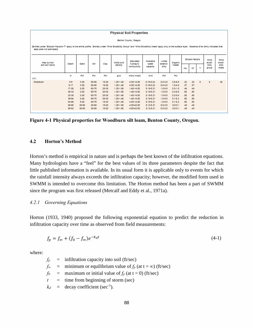
88

Figure 4-1 Physical properties for Woodburn silt loam, Benton County, Oregon.

4.2 Horton’s Method

Horton’s method is empirical in nature and is perhaps the best known of the infiltration equations. Many hydrologists have a “feel” for the best values of its three parameters despite the fact that little published information is available. In its usual form it is applicable only to events for which the rainfall intensity always exceeds the infiltration capacity; however, the modified form used in SWMM is intended to overcome this limitation. The Horton method has been a part of SWMM since the program was first released (Metcalf and Eddy et al., 1971a).

4.2.1 Governing Equations

Horton (1933, 1940) proposed the following exponential equation to predict the reduction in infiltration capacity over time as observed from field measurements:

𝑓𝑓𝑝𝑝 = 𝑓𝑓∞ + (𝑓𝑓0 − 𝑓𝑓∞)𝑚𝑚−𝑘𝑘𝑑𝑑𝑡𝑡 (4-1) where:

fp = infiltration capacity into soil (ft/sec) f∞ = minimum or equilibrium value of fp (at t = ∞) (ft/sec) f0 = maximum or initial value of fp (at t = 0) (ft/sec) t = time from beginning of storm (sec) kd = decay coefficient (sec-1).

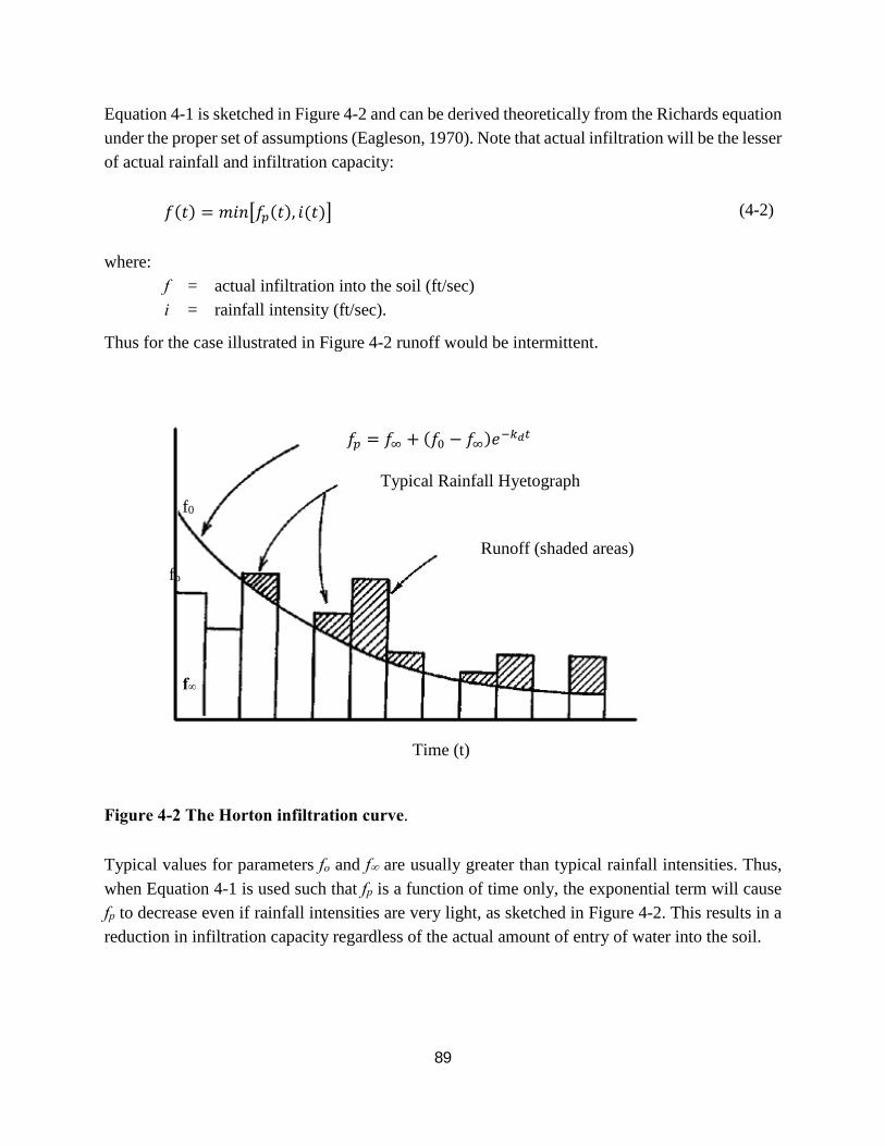
89

Equation 4-1 is sketched in Figure 4-2 and can be derived theoretically from the Richards equation under the proper set of assumptions (Eagleson, 1970). Note that actual infiltration will be the lesser of actual rainfall and infiltration capacity:

𝑓𝑓(𝑚𝑚) = 𝑚𝑚𝑚𝑚𝑚𝑚�𝑓𝑓𝑝𝑝(𝑚𝑚), 𝑚𝑚(𝑚𝑚)� (4-2) where:

f = actual infiltration into the soil (ft/sec) i = rainfall intensity (ft/sec).

Thus for the case illustrated in Figure 4-2 runoff would be intermittent.

Time (t)

fp

f0

f∞

𝑓𝑓𝑝𝑝 = 𝑓𝑓∞ + (𝑓𝑓0 − 𝑓𝑓∞)𝑚𝑚−𝑘𝑘𝑑𝑑𝑡𝑡

Typical Rainfall Hyetograph

Runoff (shaded areas)

Figure 4-2 The Horton infiltration curve. Typical values for parameters fo and f∞ are usually greater than typical rainfall intensities. Thus, when Equation 4-1 is used such that fp is a function of time only, the exponential term will cause fp to decrease even if rainfall intensities are very light, as sketched in Figure 4-2. This results in a reduction in infiltration capacity regardless of the actual amount of entry of water into the soil.

90

To correct this problem, the integrated form of Horton’s equation 4-1 is used in SWMM:

𝐹𝐹�𝑚𝑚𝑝𝑝� = � 𝑓𝑓𝑝𝑝𝑑𝑑𝑚𝑚 = 𝑓𝑓∞𝑚𝑚𝑝𝑝 +(𝑓𝑓0 − 𝑓𝑓∞)

𝑘𝑘𝑑𝑑�1 − 𝑚𝑚−𝑘𝑘𝑑𝑑𝑡𝑡𝑝𝑝�

𝑡𝑡𝑝𝑝

0

(4-3)

where F is the cumulative infiltration capacity at time tp in feet. This function is plotted in Figure 4-3 where it is assumed that actual infiltration has been equal to fp over all time t. As noted before, there will in fact be times when infiltration f is less than fp, so that the true cumulative infiltration will be:

𝐹𝐹(𝑚𝑚) = � 𝑚𝑚𝑚𝑚𝑚𝑚�𝑓𝑓𝑝𝑝, 𝑚𝑚�𝑑𝑑𝑑𝑑𝑡𝑡

0

(4-4)

Equivalent Time

tp tp1 t1

∆t F

∆F

f∞

f0

fp(tp)

fp

Figure 4-3 Cumulative infiltration F as the area under the Horton curve.

Equations 4-3 and 4-4 can thus be used to define the time tp along the Horton curve at which the next value of fp can be found. That is, F is updated with the actual infiltration f over the current time step and then the following equation, with tp as the only unknown, is solved:

91

𝐹𝐹 = 𝑓𝑓∞𝑚𝑚𝑝𝑝 +(𝑓𝑓0 − 𝑓𝑓∞)

𝑘𝑘𝑑𝑑�1 − 𝑚𝑚−𝑘𝑘𝑑𝑑𝑡𝑡𝑝𝑝� (4-5)

Once the new tp is known, the infiltration capacity fp for the next time step can be found from Equation 4-1. An additional optional parameter Fmax can be specified that limits the total volume of water that can infiltrate the soil. When cumulative infiltration exceeds this value, saturation conditions exist, and no more infiltration occurs; the land surface behaves as if it were impermeable. Thus F(t) in Equation 4-4 is not allowed to exceed Fmax.

4.2.2 Recovery of Infiltration Capacity For simulations that consist of multiple storm events over a set period of time, infiltration capacity will be regenerated (recovered) during dry weather periods. With Horton’s method, SWMM performs this function whenever a subcatchment is dry – meaning it receives no precipitation and has no ponded surface water – according to the hypothetical drying curve sketched in Figure 4-4:

𝑓𝑓𝑝𝑝 = 𝑓𝑓0 − (𝑓𝑓0 − 𝑓𝑓∞)𝑚𝑚−𝑘𝑘𝑟𝑟(𝑡𝑡−𝑡𝑡𝑤𝑤) (4-6) where:

kr = decay coefficient for the recovery curve (sec-1) tw = hypothetical projected time at which fp = f∞ on the recovery curve (sec).

New values of tp are then generated as indicated in Figure 4-4 as recovery proceeds. For example, let tpr be the tp value at which recovery begins with fr as the corresponding infiltration capacity. According to the recovery curve,

𝑓𝑓𝑟𝑟 = 𝑓𝑓0 − (𝑓𝑓0 − 𝑓𝑓∞)𝑚𝑚−𝑘𝑘𝑟𝑟�𝑡𝑡𝑝𝑝𝑟𝑟−𝑡𝑡𝑤𝑤� (4-7) one can compute tw as:

𝑚𝑚𝑤𝑤 = 𝑚𝑚𝑝𝑝𝑟𝑟 −1𝑘𝑘𝑟𝑟

𝑙𝑙𝑚𝑚 �𝑓𝑓0 − 𝑓𝑓∞

𝑓𝑓0 − 𝑓𝑓𝑟𝑟� (4-8)

92

Equivalent Time

f0

f∞

fr

f1

tpr tw1 tw tp1

𝑓𝑓𝑝𝑝 = 𝑓𝑓0 − (𝑓𝑓0 − 𝑓𝑓∞)𝑚𝑚−𝑘𝑘𝑟𝑟(𝑡𝑡−𝑡𝑡𝑤𝑤)

∆t

Figure 4-4 Regeneration (recovery) of infiltration capacity during dry time steps.

Then after a recovery time to tw1 = tpr + ∆t, the new infiltration capacity f1 is found from:

𝑓𝑓1 = 𝑓𝑓0 − (𝑓𝑓0 − 𝑓𝑓∞)𝑚𝑚−𝑘𝑘𝑟𝑟(𝑡𝑡𝑤𝑤1−𝑡𝑡𝑤𝑤) (4-9) Finally, the new equivalent time tp1 on the infiltration curve from which the infiltration process would re-start under a wet condition is:

𝑚𝑚𝑝𝑝1 =1

𝑘𝑘𝑑𝑑𝑙𝑙𝑚𝑚 �

𝑓𝑓0 − 𝑓𝑓∞

𝑓𝑓1 − 𝑓𝑓∞� (4-10)

These steps can be combined into the following equation:

𝑚𝑚𝑝𝑝1 =1

𝑘𝑘𝑑𝑑𝑙𝑙𝑚𝑚�1 − 𝑚𝑚−𝑘𝑘𝑟𝑟∆𝑡𝑡�1 − 𝑚𝑚−𝑘𝑘𝑑𝑑𝑡𝑡𝑝𝑝𝑟𝑟�� (4-11)

93

On succeeding time steps, tp1 may be substituted for tpr, and tp2 substituted for tp1, etc. Note that fp has reached its maximum value of f0 when tp = 0. Although this recovery method gives sensible results, it is somewhat unsatisfactory inasmuch as there is no dependence of infiltration recovery on evapotranspiration (ET). Drying of the soil through ET and deep infiltration should influence the recovery of infiltration capacity, but these mechanisms are replaced in SWMM by the more empirical approach just discussed.

4.2.3 Computational Scheme The detailed computational scheme for computing Horton infiltration for each subcatchment within a study area over a single time step of a simulation is presented in the sidebar below.

Computational Scheme for Horton Infiltration The following variables are assumed known at the start of each time step ∆t (sec) for the pervious subarea of each subcatchment:

i = rainfall rate (ft/sec) d = depth of ponded surface water (ft) tp = equivalent time on the Horton curve (sec)

as are the following constants: f0 = maximum (or initial) infiltration capacity (ft/sec) f∞ = minimum (or ultimate) infiltration capacity (ft/sec) kd = infiltration capacity decay coefficient (sec-1) kr = infiltration capacity recovery coefficient (sec-1) Fmax = maximum infiltration volume possible (ft).

Initially at time 0, tp = 0. The computational steps for computing the Horton infiltration rate f for a given subcatchment over a single time step of a simulation proceed as follows:

(Continued on next page)

94

1. Compute the available rainfall rate: 𝑚𝑚𝑚𝑚 = 𝑚𝑚 + 𝑑𝑑/∆𝑚𝑚.

2. If ia = 0, meaning the surface is dry, then update the current time on the Horton infiltration curve tp as follows:

𝑚𝑚𝑝𝑝 ←1

𝑘𝑘𝑑𝑑𝑙𝑙𝑚𝑚�1 − 𝑚𝑚−𝑘𝑘𝑟𝑟∆𝑡𝑡�1 − 𝑚𝑚−𝑘𝑘𝑑𝑑𝑡𝑡𝑝𝑝��

and set the infiltration rate f to 0.

3. Otherwise compute the cumulative infiltration volume from the integrated form of the Horton curve at times tp and t1 = tp + ∆t (Fp and F1, respectively) as follows:

a. If tp >= 16/kd then tp is on the flat portion of the Horton curve so

𝐹𝐹𝑝𝑝 = 𝑓𝑓∞𝑚𝑚𝑝𝑝 + 𝑓𝑓0−𝑓𝑓∞𝑘𝑘𝑑𝑑

and 𝐹𝐹1 = 𝐹𝐹𝑝𝑝 + 𝑓𝑓0∆𝑚𝑚.

b. Otherwise,

𝐹𝐹𝑝𝑝 = 𝑓𝑓∞𝑚𝑚𝑝𝑝 + (𝑓𝑓0−𝑓𝑓∞)𝑘𝑘𝑑𝑑

�1 − 𝑚𝑚−𝑘𝑘𝑑𝑑𝑡𝑡𝑝𝑝� and

𝐹𝐹1 = 𝑓𝑓∞𝑚𝑚1 +(𝑓𝑓0 − 𝑓𝑓∞)

𝑘𝑘𝑑𝑑(1 − 𝑚𝑚−𝑘𝑘𝑑𝑑𝑡𝑡1)

Limit both Fp and F1 to not exceed Fmax if a value for the latter was supplied.

4. Compute the average infiltration rate fp over the time step: 𝑓𝑓𝑝𝑝 = (𝐹𝐹1 − 𝐹𝐹𝑝𝑝)/∆𝑚𝑚.

5. If t1 > 16/kd or fp < ia then update tp to tp + ∆t.

6. Otherwise solve the nonlinear equation

𝐹𝐹𝑝𝑝 + 𝑓𝑓𝑝𝑝∆𝑚𝑚 = 𝑓𝑓∞𝑚𝑚𝑝𝑝 +(𝑓𝑓0 − 𝑓𝑓∞)

𝑘𝑘𝑑𝑑�1 − 𝑚𝑚−𝑘𝑘𝑑𝑑𝑡𝑡𝑝𝑝�

for the updated value of tp using a Newton-Raphson algorithm (Press et al., 1992).

7. Compute the actual infiltration rate f as the lesser of fp and the available rainfall rate: 𝑓𝑓 =𝑚𝑚𝑚𝑚𝑚𝑚�𝑓𝑓𝑝𝑝, 𝑚𝑚𝑚𝑚�.

The Newton-Raphson algorithm used to solve the nonlinear equation at Step 6 is included as a callable subroutine in the SWMM computer code.

95

4.2.4 Parameter Estimates

The parameters that a user must supply for each subcatchment for the Horton infiltration method are:

f0 - the maximum or initial infiltration capacity (in/hr or mm/hr), f∞ - the minimum or equilibrium infiltration capacity (in/hr or mm/hr), kd - the decay coefficient (hr-1), kr - the regeneration coefficient (days-1), and, optionally, Fmax - the maximum infiltration volume (in or mm).

Conversions between the user-supplied units of these parameters (such as in, mm or hr) and those used internally (ft and sec) are handled automatically by the program. Although the Horton equation is probably the best-known of the several infiltration equations available, there is little to help the user select values of parameters f0 and kd for a particular application. (Fortunately, some guidance can be found for the value of f∞.). Since the actual values of f0 and kd (and often f∞.) depend on the soil, vegetation, and initial moisture content, ideally these parameters should be estimated using results from field infiltrometer tests for a number of sites of the watershed and for a number of antecedent wetness conditions. An example of Horton parameters for Georgia soils is given in Table 4-2 (Rawls et al., 1976). Horton’s (1940) estimates are shown in Table 4-3. Skaggs and Khaleel (1982) provide Horton-type decay curves on the basis of theoretical estimates.

Table 4-2 Horton parameters for selected Georgia soils (Rawls et al., 1976)

Soil Type

f∞

in/hr fo

in/hr kd

hr-1

Alpha loamy sand 1.40 19.0 38.29

Carnegie sandy loam 1.77 14.77 19.64

Cowarts loamy sand 1.95 15.28 10.65

Dothan loamy sand 2.63 3.47 1.40

Fuquay pebbly loamy sand 2.42 6.24 4.70

Leefield loamy sand 1.73 11.34 7.70

Robersdale loamy sand 1.18 12.41 21.75

Stilson loamy sand 1.55 8.11 6.55

Tooup sand 1.80 23.01 32.71

96

Table 4-3 Horton parameters provided by Horton (1940)

Soil and Cover

f∞

in/hr fo

in/hr kd

hr-1

Standard agricultural (bare) 0.24 – 8.9 11.4 96

Standard agricultural (turfed) 8.2 – 11.8 36.7 48

Peat 0.82 – 11.8 13.3 108

Fine sandy clay (bare) 0.82 – 1.0 8.6 120

Fine sandy clay (turfed) 4.1 – 1.2 27.4 84 If it is not possible to use field data to find estimates of f0, f∞, and kd for each subcatchment, the following guidelines should be helpful. Often, NRCS data may be used directly. For instance, for the two upper horizons (soil layers) of Woodburn silt loam (Figure 4-1), saturated hydraulic conductivity is listed as 4 - 14 micrometers per second, or 0.6 - 2.0 in/hr (14 - 50 mm/hr). Unfortunately, this wide range in values is commonly encountered among soil survey data. Fortunately, the range also serves as a reminder that infiltration rates are notoriously variable in space as well as in time and should not be considered “exact.” Note that saturated hydraulic conductivity is the more appropriate word for parameter Ks, also termed “permeability” on older soil survey interpretation tables. Minimum Infiltration Capacity (f∞) The Horton parameter f∞ is essentially equal to saturated hydraulic conductivity, Ks, that is, f∞ ≈ Ks. The f∞ value is also the limiting infiltration rate when water is ponded on the surface, at low depths. Generalized estimates for Ks will also be discussed in conjunction with the Green-Ampt infiltration method later in this chapter and are the best source of values for f∞ in the absence of site-specific data. Alternatively, values for f∞ according to Musgrave (1955) are given in Table 4-4. To help select a value within the range given for each soil group, the user should consider the texture of the layer of least hydraulic conductivity in the profile. Depending on whether that layer is sand, loam, or clay, the f∞ value should be chosen near the top, middle, and bottom of the range respectively. For example, the data sheet for Woodburn silt loam identifies it as being in Hydrologic Soil Group B, which puts the estimate of f∞ into the range of 0.15 - 0.30 in/hr (3.8 -7.6 mm/hr), much lower than the Ks value discussed above. Examination of the texture of the layers in the soil profile indicates that they are silty in nature, suggesting that the estimate of the f∞ value should be in the low end of the range, say 0.15 - 0.20 in/hr (3.8 - 5.1 mm/hr). A sensitivity test on the f∞ value will indicate

97

the importance of this parameter to the overall result; in fact, f∞ is usually the most sensitive of the three Horton curve parameters.

Table 4-4 Values of f∞ for Hydrologic Soil Groups (Musgrave, 1955)

Hydrologic Soil Group

f∞

(in/hr)

A 0.45 - 0.30

B 0.30 - 0.15

C 0.15 - 0.05

D 0.05 - 0 Caution should be used in applying values from Table 4-4 to sandy soils (group A) since reported Ks values are often much higher. For instance, sandy soils in Florida can have Ks values from 7 to 18 in/hr (180 - 450 mm/hr) (Carlisle et al., 1981). Unless the water table rises to the surface, minimum infiltration capacity will be very high, and rainfall rates will almost always be less than f∞, leading to little or no overland flow from such soils. Decay Coefficient (kd) For any field infiltration test the rate of decrease (or “decay”) of infiltration capacity from the initial value depends on the initial moisture content. Thus the kd-value determined for the same soil will vary from test to test. It is postulated here that, if f0 is always specified in relation to a particular soil moisture condition (e.g., dry), and for moisture contents other than this the time scale is changed accordingly (i.e., time “zero” is adjusted to correspond with the constant f0), then kd can be considered a constant for the soil independent of initial moisture content. Put another way, this means that infiltration curves for the same soil, but different antecedent conditions, can be made coincident if they are moved along the time axis. Butler (1957) makes a similar assumption. Values of kd found in the literature (Overton and Meadows, 1976; Wanielista, 1978; Maidment, 1993; ASCE, 1996) range from 0.67 to 120 hr-1. Nevertheless most of the values cited appear to be in the range 3 - 6 hr-1. The evidence is not clear as to whether there is any relationship between soil texture and the kd value although several published curves seem to indicate a lower value for sandy soils. If no field data are available, an estimate of 4 hr-1 could be used. Use of such an estimate implies that, under ponded conditions, the infiltration capacity will fall 98 percent of the way towards its minimum value in the first hour, a not uncommon observation. Rates of decay of infiltration for several values of kd are shown in Table 4-5.

98

Table 4-5 Rate of decay of infiltration capacity for different values of kd

kd, hr-1

Percent of decline of infiltration capacity towards limiting value f∞ after 1 hour

2 76

3 95

4 98

5 99 Initial Infiltration Capacity (f0) The initial infiltration capacity, f0 depends primarily on soil type, initial moisture content, and surface vegetation conditions. For example, Linsley et al. (1982) present data that show, for a sandy loam soil, a 60 to 70 percent reduction in the f0 value due to wet initial conditions. They also show that lower f0 values apply for a loam soil than for a sandy loam soil. As to the effect of vegetation, Jens and McPherson (1964, pp. 20.20-20.38) list data that show that dense grass vegetation nearly doubles the infiltration capacities over those measured for bare soil surfaces. For the assumption to hold that the decay coefficient kd is independent of initial moisture content, f0 must be specified for the dry soil condition. For long-term continuous simulations SWMM automatically adjusts the effective f0 value as part of the infiltration capacity regeneration routine. However, for a single-event simulation, the user must specify the f0 value for the storm in question, which may be less than the value for dry soil conditions. Published values of f0 vary depending on the soil, moisture, and vegetation conditions for the particular test measurement. The f0 values listed in Table 4-6 can be used as a rough guide. Interpolation between the values may be required.

99

Table 4-6 Representative values for f0

A. DRY soils (with little or no vegetation): Sandy soils: 5 in/hr Loam soils: 3 in/hr Clay soils: 1 in/hr

B. DRY soils (with dense vegetation): Multiply values given in A by 2 (after Jens and McPherson, 1964).

C. MOIST soils (change from dry f0 value required for single event simulation only): Soils which have drained but not dried out (i.e., field capacity): divide values from A and B by 3. Soils close to saturation: Choose value close to f∞ value. Soils which have partially dried out: divide values from A and B by 1.5-2.5.

Regeneration Coefficient (kr) For continuous simulation, infiltration capacity will be regenerated (recovered) during dry weather according to Equation 4-6. Instead of asking the user to supply a value for kr, SWMM instead asks for an estimate of drying time Tdry in days. This is the time it takes for a saturated soil to fully recover to a dry state. Drying times are typically longer than wetting times, implying kr < kd. On well-drained porous soils (e.g., medium to coarse sands), recovery of infiltration capacity is quite rapid and could well be complete in a couple of days. For heavier soils, the recovery rate is likely to be slower, say 7 to 14 days. The choice of the value can also be related to the interval between a heavy storm and wilting of vegetation. The Green-Ampt method (discussed below in Section 4.4), bases its recovery time solely on the soil’s saturated hydraulic conductivity Ks. Adopting its approach produces the following estimate for Tdry in days:

𝑇𝑇𝑑𝑑𝑟𝑟𝑑𝑑 =3.125�𝐾𝐾𝑠𝑠

(4-12)

where Ks is expressed in in/hr. Thus this equation predicts a drying time of 2 days for a sandy soil with Ks = 2.0 in/hr versus 10 days for a clay soil with Ks of 0.1 in/hr.

100

Since mathematically, the exponential term in Equation 4-6 would require an infinite amount of time to allow infiltration capacity to return to its initial value f0, SWMM considers “full recovery” to occur when 98 percent of the difference between the initial and minimum capacities has been achieved. Thus from Equation 4-6 (for kr in days-1),

0.02(𝑓𝑓0 − 𝑓𝑓∞) = (𝑓𝑓0 − 𝑓𝑓∞)𝑚𝑚−𝑘𝑘𝑟𝑟𝑇𝑇𝑑𝑑𝑟𝑟𝑑𝑑 (4-13)

which leads to the following estimate of kr expressed in days-1:

𝑘𝑘𝑟𝑟 =−ln (0.02)

𝑇𝑇𝑑𝑑𝑟𝑟𝑑𝑑=

3.912𝑇𝑇𝑑𝑑𝑟𝑟𝑑𝑑

(4-14)

This computation of kr from a user-supplied value of Tdry and its subsequent conversion from days-

1 to sec-1 is done internally by SWMM.

4.3 Modified Horton Method A. O. Akan developed a modified version of the Horton infiltration method (Akan, 1992; Akan and Houghtalen, 2003) that has been added as a separate infiltration option in SWMM 5. The method uses the same parameters as the original Horton method but instead of tracking the time along the Horton decay curve it uses the cumulative infiltration volume in excess of the minimum infiltration rate as its state variable. It assumes that part of the infiltrating water will percolate deeper into the soil at the minimum infiltration rate (commonly taken as the soil’s saturated hydraulic conductivity). As a result, it is the difference between the actual and minimum infiltration rates that accumulates just below the surface that causes infiltration capacity to decrease with time. This method is purported to give more accurate infiltration estimates when low rainfall intensities occur.

4.3.1 Governing Equations The modified method starts with the same exponential decay equation as the original Horton method:

𝑓𝑓𝑝𝑝 = 𝑓𝑓∞ + (𝑓𝑓0 − 𝑓𝑓∞)𝑚𝑚−𝑘𝑘𝑑𝑑𝑡𝑡 (4-15)

where all symbols have been previously defined.

101

As with the original Horton method, the actual infiltration rate f is the smaller of fp and the rainfall rate i. Integrating Equation 4-15 from 0 to time t produces the following equation for the cumulative infiltration through time t:

𝐹𝐹 = 𝑓𝑓∞𝑚𝑚 +(𝑓𝑓0 − 𝑓𝑓∞)

𝑘𝑘𝑑𝑑(1 − 𝑚𝑚−𝑘𝑘𝑑𝑑𝑡𝑡) (4-16)

Solving for 𝑚𝑚−𝑘𝑘𝑑𝑑𝑡𝑡 from (4-15) and substituting into (4-16) gives:

𝐹𝐹 = 𝑓𝑓∞𝑚𝑚 +𝑓𝑓0 − 𝑓𝑓𝑝𝑝

𝑘𝑘𝑑𝑑 (4-17)

and solving for fp gives:

𝑓𝑓𝑝𝑝 = 𝑓𝑓0 − 𝑘𝑘𝑑𝑑(𝐹𝐹 − 𝑓𝑓∞𝑚𝑚) (4-18)

The last term in parenthesis is equivalent to∫ (𝑓𝑓 − 𝑓𝑓∞)𝑑𝑑𝑚𝑚𝑡𝑡0 . So one can approximate Eq. (4-18) by

𝑓𝑓𝑝𝑝 = 𝑓𝑓0 − 𝑘𝑘𝑑𝑑𝐹𝐹𝑒𝑒 (4-19)

where 𝐹𝐹𝑒𝑒 = ∑ (𝑓𝑓𝑚𝑚 − 𝑓𝑓∞)∆𝑚𝑚𝑚𝑚𝑚𝑚 and 𝑓𝑓𝑚𝑚 is the actual infiltration over a previous time interval ∆𝑚𝑚𝑚𝑚.

4.3.2 Recovery of Infiltration Capacity Regarding recovery of infiltration capacity during dry periods, one can assume that the instantaneous recovery rate is proportional to the difference between the current capacity and the maximum capacity:

𝑑𝑑𝑓𝑓𝑟𝑟 𝑑𝑑𝑚𝑚⁄ = 𝑘𝑘𝑟𝑟(𝑓𝑓0 − 𝑓𝑓𝑟𝑟) (4-20) where 𝑓𝑓𝑟𝑟 represents the infiltration capacity during recovery and 𝑘𝑘𝑟𝑟 is the same regeneration coefficient (1/sec) used in the conventional Horton method. Integrating this equation starting at some time where the infiltration capacity is 𝑓𝑓𝑟𝑟0 produces the following result for the capacity after a recovery time of t:

𝑓𝑓𝑟𝑟 = 𝑓𝑓0 − (𝑓𝑓0 − 𝑓𝑓𝑟𝑟0)𝑚𝑚−𝑘𝑘𝑟𝑟𝑡𝑡 (4-21)

102

From Eq. 4-19, the cumulative excess infiltration volume corresponding to this capacity,𝐹𝐹𝑒𝑒𝑟𝑟, would be:

𝐹𝐹𝑒𝑒𝑟𝑟 = (𝑓𝑓0 − 𝑓𝑓𝑟𝑟)/𝑘𝑘𝑑𝑑 (4-22)

and substituting 4-21 for 𝑓𝑓𝑟𝑟 gives:

𝐹𝐹𝑒𝑒𝑟𝑟 =(𝑓𝑓0 − 𝑓𝑓𝑟𝑟0)

𝑘𝑘𝑑𝑑𝑚𝑚−𝑘𝑘𝑟𝑟𝑡𝑡 (4-23)

But again from 4-19,

(𝑓𝑓0 − 𝑓𝑓𝑟𝑟0)/𝑘𝑘𝑑𝑑 = 𝐹𝐹𝑒𝑒 (4-24) so the new cumulative volume after recovery is simply:

𝐹𝐹𝑒𝑒𝑟𝑟 = 𝐹𝐹𝑒𝑒𝑚𝑚−𝑘𝑘𝑟𝑟𝑡𝑡 (4-25)

4.3.3 Computational Scheme The detailed computational scheme for computing the Modified Horton infiltration rate for each subcatchment within a study area over a single time step of a simulation is presented in the sidebar titled Computational Scheme for Modified Horton Infiltration.

4.3.4 Parameter Estimates Because the modified Horton method utilizes the same parameters as the original Horton method, the description in section 4.2.4 of how to estimate their values also applies to the modified method.

103

Computational Scheme for Modified Horton Infiltration The following variables are assumed known at the start of each time step ∆t (sec) for the pervious sub-area of each SWMM subcatchment:

i = rainfall rate (ft/sec) d = depth of ponded surface water (ft) Fe = excess infiltrated volume (ft)

as are the following constants: f0 = maximum (or initial) infiltration capacity (ft/sec) f∞ = minimum (or ultimate) infiltration capacity (ft/sec) kd = infiltration capacity decay coefficient (sec-1) kr = infiltration capacity recovery coefficient (sec-1) Fmax = maximum infiltration volume possible (optional) (ft).

Initially at time 0, Fe = 0. The following steps are used to compute the modified Horton infiltration rate f over a single time step of a simulation:

1. Compute the available rainfall rate: ia = i + d / ∆ .t

2. If ia = 0, meaning the surface is dry, then update the current excess infiltrated volume as follows:

𝐹𝐹𝑒𝑒 = 𝐹𝐹𝑒𝑒𝑚𝑚−𝑘𝑘𝑟𝑟Δ𝑡𝑡

and set the infiltration rate f to 0.

3. Else if Fe ≥ Fmax, set fp to 0. Otherwise compute a potential infiltration rate fp from

𝑓𝑓𝑝𝑝 = max (𝑓𝑓0 − 𝑘𝑘𝑑𝑑𝐹𝐹𝑒𝑒 , 𝑓𝑓∞)

4. Compute the actual infiltration rate f as the lesser of fp and the available rainfall rate:

𝑓𝑓 = min (𝑓𝑓𝑝𝑝, 𝑚𝑚𝑚𝑚)

5. If f > f∞ then update the cumulative excess infiltration volume:

𝐹𝐹𝑒𝑒 ← min (𝐹𝐹𝑒𝑒 + (𝑓𝑓 − 𝑓𝑓∞)∆𝑚𝑚, 𝐹𝐹𝑚𝑚𝑚𝑚𝑚𝑚)

104

4.4 Green-Ampt Method

The Green-Ampt equation (Green and Ampt, 1911) has received considerable attention in recent years. The original equation was for infiltration with excess water at the surface at all times. Mein and Larson (1973) showed how it could be adapted to a steady rainfall input and proposed a way in which the capillary suction parameter could be determined. Chu (1978) has shown the applicability of the equation to the unsteady rainfall situation, using data for a field catchment. The Green-Ampt method was added into SWMM III in 1981 by R.G. Mein and W. Huber (Huber et al., 1981).

4.4.1 Governing Equations The Green-Ampt conceptualization of the infiltration process is one in which infiltrated water moves vertically downward in a saturated layer, beginning at the surface (Figure 4-5). In the wetted zone the moisture content θ is at saturation θ s while the moisture content in the un-wetted zone is at some known initial level θ i.

Figure 4-5 Two-zone representation of the Green-Ampt infiltration model (after Nicklow et al., 2006).

The water velocity within the wetted zone is given by Darcy’s Law as a function of the saturated hydraulic conductivity Ks, the capillary suction head along the wetting front ψs, the depth of ponded water at the surface d, and the depth of the saturated layer below the surface Ls:

Ground Surface

Wetted Zone (θ = θs)

Non-wetted Zone (θ = θι)

Wetting Front

Ls

105

𝑓𝑓𝑝𝑝 = 𝐾𝐾𝑠𝑠 �𝑑𝑑 + 𝐿𝐿𝑠𝑠 + 𝜓𝜓𝑠𝑠

𝐿𝐿𝑠𝑠� (4-26)

The depth of the saturated layer Ls can be expressed in terms of the cumulative infiltration, F, and the initial moisture deficit to be filled below the wetting front, θ d = θ s - θi as ds /FL θ= . Substituting this into Equation 4-26 and assuming that d is small compared to the other depths gives the Green-Ampt equation for saturated conditions:

𝑓𝑓𝑝𝑝 = 𝐾𝐾𝑠𝑠 �1 +𝜓𝜓𝑠𝑠𝜃𝜃𝑑𝑑

𝐹𝐹� (4-27)

Equation 4-27 applies only after a saturated layer develops at the ground surface. Prior to this point in time the infiltration capacity will equal the rainfall intensity:

𝑓𝑓𝑝𝑝 = 𝑚𝑚 (4-28) As time increases, one can test whether saturation has been reached by solving 4-27 for F (which will be denoted as Fs) with fp set equal to i and check if this value equals or exceeds the actual cumulative infiltration F:

𝐹𝐹𝑠𝑠 =𝐾𝐾𝑠𝑠𝜓𝜓𝑠𝑠𝜃𝜃𝑑𝑑

𝑚𝑚 − 𝐾𝐾𝑠𝑠 (4-29)

Note that there is no calculation of Fs when i <= Ks, although F still gets updated during such periods. Finally, in this scheme the actual infiltration f is the same as the potential value fp:

𝑓𝑓 = 𝑓𝑓𝑝𝑝 (4-30)

The two equations are illustrated in Figure 4-6 for the situation Ks = 0.25 in/hr, ψs = 6.5 in, and θd = 0.20. The initial, flat portion of the curve corresponds to f = i, up to the point where F = Fs (Equation 4-29). The remainder of the curve corresponds to the potential rate computed with Equation 4-27. Note that the infiltration rate approaches Ks (0.25 in/hr) asymptotically.

106

Figure 4-6 Illustration of infiltration capacity as function of cumulative infiltration for the Green-Ampt method.

Equation 4-27 shows that the infiltration capacity after surface saturation depends on the infiltrated volume, which in turn depends on the infiltration rates in previous time steps. To avoid numerical errors over long time steps, the integrated form of the Green-Ampt equation is more suitable. That is, fp is replaced by dF/dt and integrated to obtain:

𝐹𝐹 = 𝐾𝐾𝑠𝑠 + 𝜓𝜓𝑠𝑠𝜃𝜃𝑑𝑑𝑙𝑙𝑚𝑚 �1 +𝐹𝐹

𝜓𝜓𝑠𝑠𝜃𝜃𝑑𝑑� (4-31)

If F1 is the known cumulative infiltration at the start of the time step and F2 the unknown cumulative infiltration at the end of the time step then one can write:

𝐹𝐹2 = 𝐶𝐶 + 𝜓𝜓𝑠𝑠𝜃𝜃𝑑𝑑𝑙𝑙𝑚𝑚(𝐹𝐹2 + 𝜓𝜓𝑠𝑠𝜃𝜃𝑑𝑑) (4-32)

where 𝐶𝐶 = 𝐾𝐾𝑠𝑠Δ𝑚𝑚 + 𝐹𝐹1 − 𝜓𝜓𝑠𝑠𝜃𝜃𝑑𝑑𝑙𝑙𝑚𝑚(𝐹𝐹1 + 𝜓𝜓𝑠𝑠𝜃𝜃𝑑𝑑) is a known constant. Equation 4-32 can be solved numerically for F2. The average infiltration capacity fp over the time step can then be computed as (𝐹𝐹2 − 𝐹𝐹1)/Δ𝑚𝑚.

0

0.2

0.4

0.6

0.8

1

0 2 4 6 8 10

F (in)

f (in

/hr)

107

4.4.2 Recovery of Infiltration Capacity

Evaporation, subsurface drainage, and moisture redistribution between rainfall events decrease the soil moisture content in the upper soil zone and increase the infiltration capacity of the soil. The processes involved are complex and depend on many factors. In SWMM a simple empirical routine (Huber et al., 1981) is used as outlined below; commonly used units are given in the equations to make the description easier to understand. Note that this procedure suffers from the same lack of relationship to ET as does the Horton recovery, discussed earlier. Infiltration is usually dominated by conditions in the uppermost layer of the soil. The thickness of this layer depends on the soil type; for a sandy soil it could be several inches, for heavy clay it would be less. The equation used to determine the thickness of the layer Lu is:

𝐿𝐿𝑢𝑢 = 4�𝐾𝐾𝑠𝑠 (4-33)

where Lu has units of inches and Ks is expressed in in/hr. Thus for a high Ks of 0.5 in/hr (12.7 mm/hr) the thickness computed by Equation 4-33 is 2.83 inches (71.8 mm). For a soil with a low hydraulic conductivity, say Ks = 0.1 in/hr (2.5 mm/hr), the computed thickness is 1.26 inches (32.1 mm). This constant thickness is different from the saturated zone thickness Ls shown in Figure 4-5 which grows over time as infiltration proceeds. In the Green-Ampt model, the initial soil moisture deficit at the start of a rainfall event determines how much infiltration capacity is available during the event itself. Recall that the moisture deficit θd is the difference between the saturated moisture content θs and the initial moisture content θi. During a dry period the moisture deficit in the upper soil zone, θdu, is regenerated, i.e., its value is increased. Thus SWMM keeps continuous track of this quantity. At the start of a simulation, θdu is set equal to the user-supplied initial value of θdmax. During a wet period when infiltration occurs at a rate f over a time step of ∆t, θdu is decreased according to:

𝜃𝜃𝑑𝑑𝑢𝑢 ← 𝜃𝜃𝑑𝑑𝑢𝑢 −𝑓𝑓Δ𝑚𝑚𝐿𝐿𝑢𝑢

(4-34)

down to a possible limiting value of 0. During a dry period it increases as follows:

𝜃𝜃𝑑𝑑𝑢𝑢 ← 𝜃𝜃𝑑𝑑𝑢𝑢 + 𝑘𝑘𝑟𝑟𝜃𝜃𝑑𝑑𝑚𝑚𝑚𝑚𝑚𝑚Δ𝑚𝑚 (4-35)

up to a maximum possible value of θdmax , where kr is a recovery constant (hr-1).

108

One can assume that the recovery constant is also dependent on Ks, such that tight, clay soils with low Ks take longer to recover than do loose, sandy soils with high Ks. The following relationship is used for kr:

𝑘𝑘𝑟𝑟 =�𝐾𝐾𝑠𝑠

75 (4-36)

where the constant 75 has units of (in-hr)1/2. Note that the time it would take a fully saturated soil to recovery to its maximum capacity is simply:

1𝑘𝑘𝑟𝑟

=75

�𝐾𝐾𝑠𝑠

hours (or 3.125/�𝐾𝐾𝑠𝑠 days). To complete the recovery process it is necessary to define the minimum amount of time that a soil must remain in recovery before any further rainfall would be considered as an independent event. This time Tr (hr) is computed as:

𝑇𝑇𝑟𝑟 =0.06𝑘𝑘𝑟𝑟

=4.5�𝐾𝐾𝑠𝑠

(4-37)

Thus when a new period of rainfall occurs after a recovery interval of at least Tr hours, the two-stage Green-Ampt infiltration process is re-started with θd = θdu and F = 0. Figure 4-7 summarizes the functional dependence of the three internally computed recovery parameters Lu, kr, and Tr on the saturated hydraulic conductivity Ks.

109

Figure 4-7 Green-Ampt recovery parameters as functions of hydraulic conductivity.

4.4.3 Computational Scheme

The detailed computational scheme for computing the Green-Ampt infiltration rate for each subcatchment within a study area over a single time step of a simulation is presented in the sidebar below.

0

2

4

6

8

10

12

14

0.01 0.10 1.00 10.00

Ks (in/hr)

Dep

th (i

n)

1

10

100

1000

Tim

e (h

r)

T

1/kr

Lu

110

Computational Scheme for Green-Ampt Infiltration Note: For ease of presentation the following description uses length units of inches and time

units of hours rather than feet and seconds which are used internally in SWMM. The following variables are assumed known at the start of each time step ∆t (hr) for the pervious subarea of each subcatchment:

i = rainfall rate (in/hr) d = depth of ponded surface water (in) θd = soil moisture deficit at the start of the current rainfall event θdu = soil moisture deficit in the upper soil recovery zone F = cumulative infiltrated volume (in) T = recovery time remaining before the next event can begin (hr).

as are the following constants: Ks = saturated hydraulic conductivity (in/hr) ψs = suction head at the wetting front (in) θdmax = maximum soil moisture deficit Lu = depth of upper soil recovery zone (in) kr = moisture deficit recovery constant (hr-1) Tr = minimum recovery time before a new rainfall event occurs (hr).

The latter three constants are derived from Ks as described previously. Initially at time 0, θd = θdu = θdmax, F = 0, T = 0 and the surface is in an unsaturated state. The computational scheme for evaluating the Green-Ampt infiltration rate f over each time step follows two separate paths, depending on whether the surface layer is in a saturated state or not. The scheme for the unsaturated state proceeds as follows:

1. Compute the available rainfall rate: 𝑚𝑚𝑚𝑚 = 𝑚𝑚 + 𝑑𝑑/Δ𝑚𝑚.

2. Decrease the recovery time remaining before the next storm event: 𝑇𝑇 ← 𝑇𝑇 − ∆𝑚𝑚.

(Continued on next page)

111

3. If the available rainfall rate is zero (ia = 0) then:

a. Set f = 0.

b. Recover upper zone moisture deficit θdu and cumulative infiltration F: ∆𝜃𝜃 = 𝑘𝑘𝑟𝑟𝜃𝜃𝑑𝑑𝑚𝑚𝑚𝑚𝑚𝑚Δ𝑚𝑚 𝜃𝜃𝑑𝑑𝑢𝑢 ← 𝜃𝜃𝑑𝑑𝑢𝑢 + Δ𝜃𝜃 𝐹𝐹 ← 𝐹𝐹 − Δ𝜃𝜃𝐿𝐿𝑢𝑢

c. If the minimum recovery time has expired (T ≤ 0), then set θd = θdu and F = 0 to mark the beginning of a new rainfall event.

4. If the available rainfall rate does not exceed the saturated hydraulic conductivity (ia ≤ Ks) then:

a. Set 𝑓𝑓 = 𝑚𝑚𝑚𝑚.

b. Update cumulative infiltration:

Δ𝐹𝐹 = 𝑚𝑚𝑚𝑚Δ𝑚𝑚 𝐹𝐹 ← 𝐹𝐹 + ∆𝐹𝐹 𝜃𝜃𝑑𝑑𝑢𝑢 ← 𝜃𝜃𝑑𝑑𝑢𝑢 − Δ𝐹𝐹/𝐿𝐿𝑢𝑢

5. If the available rainfall rate ia exceeds Ks then:

a. Set T = Tr.

b. Compute the volume needed to saturate the surface layer, Fs, from Equation 4-29:

𝐹𝐹𝑠𝑠 =𝐾𝐾𝑠𝑠𝜓𝜓𝑠𝑠𝜃𝜃𝑑𝑑

𝑚𝑚𝑚𝑚 − 𝐾𝐾𝑠𝑠

c. If the surface layer is currently saturated (𝐹𝐹 ≥ 𝐹𝐹𝑠𝑠) then use the procedure for saturated conditions described below to compute f.

d. If 𝐹𝐹 + 𝑚𝑚𝑚𝑚∆𝑚𝑚 < 𝐹𝐹𝑠𝑠 (i.e., the surface remains unsaturated) then set f = ia and update F and θdu as in Step 4b above.

(Continued on next page)

112

e. Otherwise the surface becomes saturated during the time step. Solve Equation 4-32 for F2 using Fs for F1 and ∆t – (Fs – F) / ia for ∆t (i.e., the portion of the original time step over which saturated conditions exist). Then set:

∆𝐹𝐹 = 𝐹𝐹2 − 𝐹𝐹 𝐹𝐹 = 𝐹𝐹2 𝜃𝜃𝑑𝑑𝑢𝑢 ← 𝜃𝜃𝑑𝑑𝑢𝑢 − Δ𝐹𝐹/𝐿𝐿𝑢𝑢 𝑓𝑓 = Δ𝐹𝐹/Δ𝑚𝑚

The computational steps used for saturated conditions are as follows:

1. Compute the available rainfall rate: 𝑚𝑚𝑚𝑚 = 𝑚𝑚 + 𝑑𝑑/Δ𝑚𝑚.

2. Reset T = Tr.

3. Solve Equation 4-32 for F2 with F1 = F.

4. Set ∆F = F2 – F.

5. If Δ𝐹𝐹 > 𝑚𝑚𝑚𝑚∆𝑚𝑚 then set ∆𝐹𝐹 = 𝑚𝑚𝑚𝑚∆𝑚𝑚 and change the current surface layer condition to unsaturated.

6. Update the following:

𝐹𝐹 ← 𝐹𝐹 + ∆𝐹𝐹

𝜃𝜃𝑑𝑑𝑢𝑢 ← 𝜃𝜃𝑑𝑑𝑢𝑢 − Δ𝐹𝐹/𝐿𝐿𝑢𝑢

𝑓𝑓 = Δ𝐹𝐹/Δ𝑚𝑚

Note that in both of these paths, θdu is not allowed to drop below 0 nor exceed θdmax. Also, a Newton-Raphson procedure (Press et al., 1992) is used to solve the integrated form of the Green-Ampt Equation 4-32 at Step 5e of the unsaturated procedure and at Step 3 of the saturated procedure.

113

4.4.4 Parameter Estimates

The soil parameters that a user must supply for each subcatchment for the Green-Ampt infiltration method are:

• Ks - the saturated hydraulic conductivity (in/hr or mm/hr),

• ψs - the suction head at the wetting front (in or mm),

• θdmax - the maximum moisture deficit available (volume of dry voids per volume of soil).

Conversions between the user-supplied units of these parameters (in (or mm) and hr) and those used internally (ft and sec) are handled automatically by the program. Saturated Hydraulic Conductivity (Ks) Probably the best single source for estimates of saturated hydraulic conductivity (Ks) and suction head (ψs) for a wide range of soils – and one that makes use of the Green-Ampt method relatively attractive – is the data by Rawls et al. (1983), shown in Table 4-7. These data were derived from measurements made on roughly 5000 soils across the United States and while they will never be truly site specific, they are certainly consistent and defensible. Although there is considerable variation in the parameter estimates, a good first approximation may be made using the table. Values of hydraulic conductivity may also be used for estimates of the Horton parameter f∞. But the range of values shown for porosity and suction head (the authors do not provide ranges for Ks) should be a warning about placing too much faith in such generalized estimates. The NRCS Soil Survey Physical Data (see Figure 4-1) values for hydraulic conductivity could also be used as a preliminary estimate. A better guide for the Ks values is as given for parameter f∞ for the Horton equation; theoretically these parameters (i.e., f∞ and Ks) should be equal for the same soil. Note that, in general, the range of Ks values encountered will be of the order of tenths of an inch per hour. Another source of conductivity estimates is the regression equation developed by Saxton and Rawls (2006) that predicts Ks from the sand, clay and organic matter content of a soil. See Section 5.5.2 of the Groundwater chapter for more details.

114

Table 4-7 Green-Ampt parameters for different soil classes (Rawls et al., 1983) (Numbers in parentheses are ± one standard deviation from the parameter value shown.)

Soil Class

Porosity, φ

Effective

Porosity, φe*

Wetting Front Suction Head,

ψs (in)

Saturated Hydraulic

Conductivity, Ks (in/hr)

Sand 0.437 (0.374–0.500)

0.417 (0.354–0.480)

1.95 (0.38–9.98)

4.74

Loamy sand 0.437 (0.363–0.506)

0.401 (0.329–0.473)

2.41 (0.53–11.00)

1.18

Sandy loam 0.453 (0.351–0.555)

0.412 (0.283–0.541)

4.33 (1.05–17.90)

0.43

Loam 0.463 (0.375–0.551)

0.434 (0.334–0.534)

3.50 (0.52–23.38)

0.13

Silt loam 0.501 (0.420–0.582)

0.486 (0.394–0.578)

6.57 (1.15–37.56)

0.26

Sandy clay loam

0.398 (0.332–0.464)

0.330 (0.235–0.425)

8.60 (1.74–42.52)

0.06

Clay loam 0.464 (0.409–0.519)

0.309 (0.279–0.501)

8.22 (1.89–35.87)

0.04

Silty clay loam

0.471 (0.418–0.524)

0.432 (0.347–0.517)

10.75 (2.23–51.77)

0.04

Sandy clay 0.430 (0.370–0.490)

0.321 (0.207–0.435)

9.41 (1.61–55.20)

0.02

Silty clay 0.479 (0.425–0.533)

0.423 (0.334–0.512)

11.50 (2.41–54.88)

0.02

Clay 0.475 (0.427–0.523)

0.385 (0.269–0.501)

12.45 (2.52–61.61)

0.01

*Effective porosity is the difference between the porosity φ and the residual moisture content φr that remains after a saturated soil is allowed to drain thoroughly.

115

Urban soils are usually highly disturbed (Pitt et al., 1999, 2001; Pitt and Voorhees, 2000). Construction has often occurred on or nearby the locations in question, and soils may be compacted from their natural state. Alternatively, soils are sometimes imported for horticultural purposes. Such imported soils (e.g., for lawns) may exhibit relatively high infiltration rates. The parameter estimates discussed previously are based on data for undisturbed soils, e.g., using Natural Resources Conservation Service (NRCS) data. Parameters for natural, undisturbed soils are likely to overestimate the infiltration characteristics for urban soils. Modelers should bear in mind that only site-specific infiltrometer and/or soil physics tests can determine local infiltration properties, and that high spatial variability is the rule, rather than the exception. Suction Head (ψs) The suction head, ψs (also referred to as capillary tension), is perhaps the most difficult parameter to measure. It can be derived from soil moisture - conductivity data (Mein and Larsen, 1973) of the type shown in Figures 5-5 in Chapter 5 for groundwater. Unfortunately, such detailed data are rare for most soils. Fortunately the results obtained for Green-Ampt infiltration are not highly sensitive to the estimate of ψs (Brakensiek and Onstad, 1977). An excellent local data source can often be found in Soil Science departments at state universities. Tests are run on a variety of soils found within the state, including soil moisture versus soil tension data, from which ψs can be derived. For example, Carlisle et al. (1981) provide such data for Florida soils along with information on Ks, bulk density, and other physical and chemical properties. Approximate values may also be found from several authors: Mein and Larsen (1973), Brakensiek and Onstad (1977), Clapp and Hornberger (1978), Chu (1978), Rawls et al. (1983). Published values vary considerably and conflict; however, a range of 2 to 15 inches (50 to 380 mm) covers virtually all soil textures. But as with Ks, probably the best single source for estimates for capillary suction (ψs) is the data by Rawls et al. (1983) listed in Table 4-7. Brakensiek et al. (1981) noted that ψs was highly correlated with hydraulic conductivity over all soil classes. Using nonlinear regression on the average values for these two variables listed in Table 4-7 produces the following relationship for KS in in/hr and ψs in inches:

𝜓𝜓𝑠𝑠 = 3.237𝐾𝐾𝑆𝑆−0.328 (R2 = 0.9) (4-38)

116

Maximum Moisture Deficit (θdmax) The maximum moisture deficit, θdmax is defined as the difference between the moisture content at saturation and at the start of the simulation. Because this parameter is the most sensitive of the three parameters for estimates of runoff from pervious areas (Brakensiek and Onstad, 1977), some care should be taken in determining the best θdmax value to use. The saturated moisture content is approximately equal to the soil’s porosity φ (i.e., the fraction of voids), assuming one ignores the 5 - 10% of trapped air that typically exists at saturation. After a saturated soil is allowed to drain thoroughly, the residual moisture content that remains is φr. The effective porosity φe is defined as φ −φr and can be used to represent θdmax for dry antecedent conditions. Typical values of φe are included in the Rawls et al. (1983) data set listed in Table 4-7. Sandy soils tend to have lower porosities than clay soils, but drain to lower moisture contents between storms because the water is not held so strongly in the soil pores. Consequently, values of θdmax for dry antecedent conditions tend to be higher for sandy soils than for clay soils. Table 4-8, derived from Clapp and Hornberger (1973), is another source of θdmax values for various soil types.

Table 4-8 Typical values of θdmax for various soil types.

Soil Texture Typical θdmax at Soil Wilting Point

Sand 0.34

Sandy Loam 0.33

Silt Loam 0.32

Loam 0.31

Sandy Clay Loam 0.26

Clay Loam 0.24

Clay 0.21

117

These θdmax values would be suitable for input for long term continuous simulation; the soil type selected should correspond to the surface layer for the particular subcatchment. For single event simulation the values of Table 4-8 would apply only to very dry antecedent conditions. For moist or wet antecedent conditions lower values of θdmax should be used. When estimating the particular value it should be borne in mind that sandy soils drain more quickly than clayey soils, i.e., for the same time since the previous event, the θdmax value for a sandy soil will be closer in value to that of Table 4-8 than it would be for a clayey soil. Another estimate for θdmax may be based on the NRCS Soil Survey Physical Data as “Available Moisture Capacity” in/in of soil (dimensionless fraction), which is defined as the difference between field capacity and the wilting point. Thus, it is an underestimate of the maximum θd value. Furthermore, Available Moisture Capacity values listed may exhibit similar variability (or lack thereof) as for hydraulic conductivity estimates discussed earlier, but these values are at least specific to the soil in question. For instance, for the Woodburn silt loam illustrated in Figure 4-1, θdmax might be at the high end of the range of 0.19 – 0.24 for the surface layer (considerably less than the generic value of 0.32 for silt loam in Table 4-8 or the range of 0.394 to 0.578 given in Table 4-7). Finally, the initial moisture deficit can be related to another very general measure of a soil: its storage capacity, S, which can be expressed as:

𝑆𝑆 = 𝑑𝑑𝑤𝑤𝑡𝑡𝜃𝜃𝑑𝑑𝑚𝑚𝑚𝑚𝑚𝑚 (4-39) where dwt is the depth to the sub-surface water table. Estimates of soil storage capacity, S, are available using the Curve Number method, discussed below. That is, S is a function of the curve number (Section 4.5.4), for which a vast literature is available. If depth to water table is known, or if typical depths are given for a soil on its Soil Survey Interpretation data, then Equation 4-39 may be solved for θdmax.

4.5 Curve Number Method

The Curve Number infiltration method is new to SWMM 5. It is based on the widely used SCS (Soil Conservation Service, now known as the NRCS – Natural Resource Conservation Service) curve number method for evaluating rainfall excess. First developed in 1954, the method is embodied in the widely used TR-20 and TR-55 computer models (NRCS, 1986) as well as most hydrology handbooks and textbooks (e.g., Bedient et al., 2013). It was added into SWMM to take advantage of its familiarity to most practicing engineers and the availability of tabulated curve

118

numbers for a wide range of land use and soil groups. The original curve number method is a combined loss method that lumps together all losses due to interception, depression storage, and infiltration to predict the total rainfall excess from a rainfall event. The SWMM uses a modified, incremental form of the method that accounts only for infiltration losses, since the other abstractions are modeled separately. Other incremental applications of the curve number method have been proposed by Chen (1975), Aron et al. (1977) and Akan and Houghtalen (2003).

4.5.1 Governing Equations In its classic form, the Curve Number model uses the following equation to relate total event runoff Q (in) to total event precipitation P (in) (Haan et al., 1994; McCuen, 1998; Bedient et al., 2013; NRCS, 2004b):

𝑄𝑄 =𝑃𝑃2

𝑃𝑃 + 𝑆𝑆𝑚𝑚𝑚𝑚𝑚𝑚 (4-40)

where Smax = the soil’s maximum moisture storage capacity (inches). Smax can also be thought of as the difference in water volume contained in a fully saturated soil versus a fully drained soil. In this sense it is similar to the maximum moisture deficit parameter θdmax used in the Green-Ampt model, except it is expressed on a volumetric basis rather than as a fraction (see Equation 4-39). Smax is derived from a tabulated “curve number” CN that varies with soil type and antecedent conditions:

𝑆𝑆𝑚𝑚𝑚𝑚𝑚𝑚 =1000𝐶𝐶𝐶𝐶

− 10 (4-41)

It should be emphasized that Equation 4-40 and subsequent equations use units of inches. Curve numbers for various soil types and land covers are tabulated in the NRCS’s National Engineering Handbook (NRCS, 2004a) and in many text books. In the formal SCS method, Equation 4-40 is written with P replaced by P – Ia where Ia is an initial abstraction (in) that accounts for the volume of rainfall captured by vegetative interception, filling of depression storage, and initial soil wetting. Because SWMM already accounts for these phenomena through its depression storage parameter, dp, this refinement is not included here. Assuming that all rainfall that does not run off is lost to infiltration (i.e., P – Q = F), Equation 4-40 can be extended to predict total (cumulative) infiltration F (in) as:

119

𝐹𝐹 = 𝑃𝑃 −𝑃𝑃2

𝑃𝑃 + 𝑆𝑆𝑚𝑚𝑚𝑚𝑚𝑚 (4-42)

For a continuous model like SWMM, Equation 4-42 can be applied in an incremental fashion to compute an infiltration rate f at each time step. Let P1 and F1 be the cumulative precipitation and infiltration, respectively, at the start of the time step. At the end of the time step:

𝑃𝑃2 = 𝑃𝑃1 + 𝑚𝑚Δ𝑚𝑚 (4-43)

and

𝐹𝐹2 = 𝑃𝑃2 −𝑃𝑃2

2

𝑃𝑃2 + 𝑆𝑆𝑒𝑒 (4-44)

where P2 and F2 are the cumulative precipitation and infiltration values, respectively, at the end of a time step ∆t (hr), i (in/hr) is the rainfall rate over the time step, and Se is the moisture storage capacity at the start of the rainfall event to which the time step belongs. For a single event simulation, Se equals Smax but may be lower when moisture storage capacity depletion and recovery occur over a longer simulation period as discussed in the next section. The infiltration rate f (ft/sec) can then be computed as:

𝑓𝑓 = (𝐹𝐹2 − 𝐹𝐹1)/Δ𝑚𝑚 (4-45) and the cumulative values get updated to P1 = P2 and F1 = F2 to prepare for the next time step. Note that as it stands, this model would not allow for any infiltration of ponded water when there is a period of no rainfall within an event. To overcome this limitation it is assumed that the infiltration rate for such periods remains the same as in the immediately preceding period. Also, when overland flow re-routing occurs (see Section 3.6), the rainfall rate i in Equation 4-43 does not include the additional re-routed flow.

4.5.2 Recovery of Storage Capacity As with the other infiltration methods discussed, a soil’s moisture storage capacity is depleted during wet periods and replenished during dry periods. To model this behavior with the Curve

120

Number method, the variable S is introduced to track the remaining storage capacity (i.e., moisture deficit) over time. It is analogous to the state variable θdu used in the Green-Ampt method. Initially, S = Smax. Whenever infiltration at rate f occurs over a time step ∆t, S is reduced by f∆t. During a period with no infiltration S is assumed to be replenished at a rate proportional to Smax:

𝑆𝑆 ← 𝑆𝑆 + 𝑘𝑘𝑟𝑟𝑆𝑆𝑚𝑚𝑚𝑚𝑚𝑚∆𝑚𝑚 (4-46) where kr is a storage capacity recovery constant (hr-1). This recovery expression has the same form as used in the Green-Ampt model and the coefficient kr has a similar meaning in both models. Because the Curve Number method was originally meant to be applied to single, discrete rainfall events, a mechanism is needed to define when separate events occur. At the start of a new event, the cumulative variables P and F are reset to 0 and Se is set equal to the current remaining storage capacity S. Once again borrowing from the Green-Ampt method, a period of Tr hours without rainfall must occur before the next rainfall period is deemed to begin a new event. Tr is assumed to be related to the recovery constant kr through Equation 4-25 which is repeated here:

𝑇𝑇𝑟𝑟 =0.06𝑘𝑘𝑟𝑟

(4-47)

4.5.3 Computational Scheme The detailed computational scheme for computing Curve Number infiltration for each subcatchment within a study area over a single time step of a simulation is presented in the sidebar below.

121

Computational Scheme for Curve Number Infiltration Note: For ease of presentation the following description uses length units of inches and time

units of hours rather than feet and seconds which are used internally in SWMM. The following variables are assumed known at the start of each time step ∆t (hr) for the pervious subarea of each subcatchment:

i = rainfall rate over the current time step (in/hr) d = depth of ponded surface water (in) P1 = cumulative rainfall for the current rainfall event (in) Se = soil moisture storage capacity at the start of the current rainfall event (in) S = soil moisture storage capacity remaining (in) F1 = cumulative infiltration volume (in) T = time since the last period with rainfall (hr).

as are the following constants: Smax = maximum moisture storage capacity as computed from the curve number

(in) kr = storage capacity recovery constant (hr-1) Tr = minimum recovery time before a new rainfall event can occur (hr).

Initially at time 0, P1 = 0, Se = S = Smax, F1 = 0, and T = Tr. The computational steps for computing the Curve Number infiltration rate f for a given subcatchment over a single time step of a simulation proceed as follows:

1. If there is rainfall (i > 0) then:

a. If a new event has begun (𝑇𝑇 ≥ 𝑇𝑇𝑟𝑟) then reset the following variables: P1 = 0, F1 = 0, and Se = S.

b. Reset the time since the last rainfall: T = 0.

c. Compute cumulative rainfall (P2) and infiltration (F2) at the end of the time step:

𝑃𝑃2 = 𝑃𝑃1 + 𝑚𝑚∆𝑚𝑚

𝐹𝐹2 = 𝑃𝑃2 −𝑃𝑃2

2

𝑃𝑃2 + 𝑆𝑆𝑒𝑒

(Continued on next page)

122

4.5.4 Parameter Estimates There are only two parameters required for each subcatchment using the Curve Number infiltration method:

• the curve number

• the drying time (i.e., the time it takes a fully saturated soil to recover to a dry state).

The curve number is used to compute the maximum soil moisture storage capacity (Smax) using Equation 4-41. The drying time Tdry in days is used to compute the regeneration constant kr in hours-1 as:

𝑘𝑘𝑟𝑟 =1

24𝑇𝑇𝑑𝑑𝑟𝑟𝑑𝑑 (4-48)

The minimum inter-event recovery time Tr is then computed from kr using Equation 4-47.

d. Compute a potential infiltration rate:

𝑓𝑓𝑝𝑝 = (𝐹𝐹2 − 𝐹𝐹1)∆𝑚𝑚.

e. Update cumulative rainfall and infiltration:

P1 = P2

F1 = F2.

2. If there is no rainfall then increase the inter-event time (𝑇𝑇 ← 𝑇𝑇 + ∆𝑚𝑚) and set the potential infiltration rate to the rate from the previous time period (fp = f).

3. If there is some potential infiltration (fp > 0) then:

a. Limit the actual infiltration rate to the maximum available rate:

𝑓𝑓 = 𝑚𝑚𝑚𝑚𝑚𝑚�𝑓𝑓𝑝𝑝, 𝑚𝑚 + 𝑑𝑑/∆𝑚𝑚�

b. Reduce the soil moisture storage capacity:

𝑆𝑆 ← 𝑚𝑚𝑎𝑎𝑚𝑚[𝑆𝑆 − 𝑓𝑓∆𝑚𝑚, 0].

4. Otherwise regenerate soil moisture storage capacity:

𝑆𝑆 ← 𝑚𝑚𝑚𝑚𝑚𝑚[𝑆𝑆 + 𝑘𝑘𝑟𝑟𝑆𝑆𝑚𝑚𝑚𝑚𝑚𝑚∆𝑚𝑚, 𝑆𝑆𝑚𝑚𝑚𝑚𝑚𝑚]

123

A highly structured method for estimating curve numbers is provided by the NRCS (NRCS, 2004a; McCuen, 1998, Bedient et al., 2013 and virtually every hydrology text). Such estimates are embedded in engineering practice through Table 4-9 in which curve number values are given as function of land use and soil Hydrologic Soil Group (A through D). Hydrologic Soil Group is provided on the NRCS Soil Survey data discussed in Section 4.1. For instance, the Woodburn silt loam of Figure 4-1 is in Hydrologic Soil Group B. There are several things to keep in mind when using curve numbers from Table 4-9. First, these curve numbers apply only to normal antecedent moisture conditions (AMC II). For AMC I (low moisture) or AMC III (high moisture) the following adjustments can be made to the tabulated values (NRCS, 2004a):

𝐶𝐶𝐶𝐶𝐼𝐼 =4.2𝐶𝐶𝐶𝐶𝐼𝐼𝐼𝐼

10 − 0.058𝐶𝐶𝐶𝐶𝐼𝐼𝐼𝐼 (4-49)

𝐶𝐶𝐶𝐶𝐼𝐼𝐼𝐼𝐼𝐼 =23𝐶𝐶𝐶𝐶𝐼𝐼𝐼𝐼

10 − 0.13𝐶𝐶𝐶𝐶𝐼𝐼𝐼𝐼 (4-50)

where CNi refers to the curve number for antecedent moisture condition i. For long-term simulations the AMC I curve number should be used to allow the soil to reach its maximum possible moisture retention capacity during extended dry periods. Second, the urban land use descriptions included in Table 4-9 lump together the pervious and impervious portions of the subcatchment area to which a curve number is assigned. This means that the subcatchment in question must be modeled as being completely pervious, with no partitioning into separate pervious and impervious areas as is normally done in SWMM (refer to Section 3.3). Otherwise too much runoff will be generated. If one wants to continue to partition their subcatchments into pervious and impervious areas, they will have to either adjust the curve numbers taken from Table 4-9 to remove the effects of imperviousness or find another source of curve numbers, such as from calibration against field measurements (see Shuster and Pappas, 2011).

124

Table 4-9 Runoff curve numbers for selected land uses (NRCS, 2004a) (For antecedent moisture condition II)

Hydrologic Soil Group

Land Use Description A B C D

Cultivated land1

Without conservation treatment 72 81 88 91

With conservation treatment 62 71 78 81

Pasture or range land

Poor condition 68 79 86 89

Good condition 39 61 74 80

Meadow

Good condition 30 58 71 78

Wood or forest land

Thin stand, poor cover, no mulch 45 66 77 83

Good cover2 25 55 70 77

Open spaces, lawns, parks, golf courses, cemeteries, etc.

Good condition: grass cover on 75% or more of the area 39 61 74 80

Fair condition: grass cover on 50 – 75% of the area 49 69 79 84

Commercial and business areas (85% impervious) 89 92 94 95

Industrial districts (72% impervious) 81 88 91 93

Residential3

Average lot size Average % impervious4

1/8 ac or less 65 77 85 90 92

1/4 ac 38 61 75 83 87

1/3 ac 30 57 72 81 86

1/2 ac 25 54 70 80 85

1 ac 20 51 68 79 84

Paved parking lots, roofs, driveways, etc.5 98 98 98 98

Streets and roads

Paved with curbs and storm sewers5 98 98 98 98

Gravel 76 85 89 91

Dirt 72 82 87 89 (Footnotes appear on following page)

125

Estimates of a soil’s drying time have been discussed previously in conjunction with both the Horton regeneration constant in Section 4.2.4 and the Green-Ampt recovery process in Section 4.3.2. It was suggested that the drying time Tdry in days could be related to a soil’s saturated hydraulic conductivity Ks in in/hr as follows:

𝑇𝑇𝑑𝑑𝑟𝑟𝑑𝑑 =3.125�𝐾𝐾𝑠𝑠

(4-51)

where estimates of Ks based on soil type can be found from Table 4-7.

4.6 Numerical Example

Because the four infiltration methods discussed in this chapter have very different formulations, it is interesting to compare the results they produce for a specific set of modeling conditions. Each method was used to simulate infiltration over a relatively flat, completely pervious subcatchment containing a well-drained Group B soil. The subcatchment properties, rainfall event, and infiltration parameters for each method are listed in Table 4-10. The infiltration parameters were chosen to have each method produce about the same amount of runoff for the design storm yet be within the normal ranges discussed in previous sections of this chapter.

Footnotes for Table 4-9: 1. For a more detailed description of agricultural land use curve numbers, refer to the

NRCS (2004a) National Engineering Handbook, Chapter 9, “Hydrologic Soil-Cover Complexes”.

2. Good cover is protected from grazing and litter and brush cover soil. 3. Curve numbers are computed assuming that the runoff from the house and driveway is

directed toward the street with a minimum of roof water directed to lawns where additional infiltration could occur.

4. The remaining pervious areas (lawn) are considered to be in good pasture condition for these curve numbers.

5. In some warmer climates of the country a curve number of 95 may be used.

126

Table 4-10 Parameters used in example comparison of infiltration methods

Item Parameter Value Subcatchment Percent Impervious 0

Percent Slope 0.5

Width (ft) 140

Roughness 0.1

Depression Storage (in) 0.05

Rainfall Event Duration (hr) 6.0

Total Depth (in) 2.0

Time-to-Peak / Duration 0.375

Evaporation (in/hr) 0

Horton Infiltration Initial Capacity (in/hr) 1.2

Ultimate Capacity (in/hr) 0.1

Decay Coefficient (hr-1) 2.0

Drying Time (days) 7.0

Green-Ampt Infiltration Saturated Hydraulic Conductivity (in/hr) 0.1

Suction Head (in) 2.0

Initial Moisture Deficit 0.2

Curve Number Infiltration Curve Number 80

Drying Time (days) 7.0

Figure 4-8 shows the infiltration rates obtained with each infiltration method under these conditions. The numbers in the chart’s legend are the fraction of rainfall that becomes runoff for each method. Even though similar amounts of runoff are produced, the methods display distinctly different infiltration patterns over time. These patterns are influenced not only by the parameters that were chosen for each method, but also by the temporal pattern of rainfall intensity that occurs during an event.

127

Figure 4-8 Infiltration rates produced by different methods for a 2-inch rainfall event. (Numbers in parentheses are the fraction of rainfall that becomes runoff.)

128

Chapter 5 – Groundwater

5.1 Introduction Because SWMM was originally developed to simulate combined sewer overflows in urban catchments, the fate of infiltrated water was considered insignificant. Since its development, however, SWMM has been used on areas ranging from highly urban to completely rural. Many undeveloped, and even some developed areas, especially in areas like south Florida, are very flat with high water tables, and their primary drainage pathway is through the surficial groundwater aquifer and the unsaturated zone above it, rather than by overland flow. In these areas, underlain by permeable sub-soils and dynamic water tables, a storm will cause a rise in the water table and subsequent slow release of groundwater back to the receiving water (Capece et al., 1984). For this case, the fate of the infiltrated water is a highly significant part of the local water cycle. By assuming that the infiltration is lost from the system, an important part of the subsurface flow system is not properly described (Gagliardo, 1986). In unlined channels and natural streams, the complete water balance in the near surface soils needs to be maintained in order to compute baseflow. Saturated zone outflow is a critical component of models such as HSPF (Bicknell et al. 1997) for realistic simulation of streamflow in areas in which overland flow rarely exists, which is characteristic of most non-urban soils except for very clayey areas. Groundwater discharge accounts for the time-delayed recession curve that is prevalent in most non-urban watersheds (Fetter, 1980). This process cannot, however, be satisfactorily modeled by surface runoff methods alone. By modifying infiltration parameters to account for subsurface storage, attempts have been made to overcome the fact that SWMM assumes infiltration is lost from the system (Downs et al., 1986). Although the modeled and measured peak flows matched well, the volumes did not match well, and the values of the infiltration parameters were unrealistic. Some research on the nature of the soil storage capacity has been done in south Florida (SFWMD, 1984). However, it was directed towards determining an initial storage capacity for the start of a storm. Another need is to combine the groundwater discharge hydrograph with the surface runoff hydrograph and determine when the water table will rise to the surface. Additionally, a threshold saturated water zone storage is needed (corresponding to the bottom of a stream channel), below which no saturated zone outflow will occur. This is required to simulate dry watershed conditions. Finally, it is also desirable to simulate bank storage, the movement of water from a stream channel into the saturated groundwater zone when the stream water level is higher than the adjacent groundwater table.

129

To address these needs, a simple, two-zone groundwater routine was incorporated into version 4 of SWMM in 1987 by W. Huber and B. Cunningham, based on Gagliardo’s (1986) MS thesis. The intent was to develop a physically-based model whose parameters were based on readily available soil properties. The current version of SWMM has reformulated and simplified the original model’s governing equations and solution procedure. This section describes the theory and limitations of these methods.

5.2 Governing Equations SWMM analyzes groundwater flow for each subcatchment independently. It represents the subsurface region beneath a subcatchment as consisting of an unsaturated upper zone that lies above a lower saturated zone, illustrated in Figure 5-1. The height of the water table (i.e., the boundary between the two zones) changes with time depending on the rates of inflow and outflow of the saturated lower zone. This variable volume, two-zone configuration is similar to that used by Dawdy and O’Donnell (1965) and serves as an alternative pathway for infiltrated rainfall to pass between a subcatchment and a point in the conveyance system in an attenuated and delayed fashion.

Upper Zone

Lower Zone

dU

dL

EG

EB

fI fE

fE

fL

fU

fG

Figure 5-1 Definitional sketch of the two-zone groundwater model.

Flow from the unsaturated upper zone to the saturated lower zone is controlled by a percolation equation for which parameters may either be estimated or calibrated, depending on the availability of the necessary soils data. The upper zone receives vertical inflow from infiltrating rainfall as described in Chapter 4 and can also lose moisture through evapotranspiration. For time steps where the water table has risen to the surface (reducing the unsaturated zone volume to zero), infiltration ceases and runoff is produced by saturation excess.

130

Losses and outflow from the lower zone consist of deep percolation, saturated zone evapotranspiration, and lateral groundwater flow. The latter is a user-defined power function of water table stage and depth of water in the receiving node of the conveyance system. If the water elevation at the node is higher than the saturated zone water table, back-flow (bank storage) can occur into the saturated zone. This two-zone representation of surface runoff-groundwater interaction is modeled as follows (refer to Figure 5-1). The ground surface has a known elevation (relative to some fixed reference) of EG (ft) and the bottom of the saturated zone has a known elevation of EB (ft). The unsaturated upper zone has a varying moisture content denoted as θ. The lower zone is completely saturated, and therefore its moisture content is fixed at the soil porosity φ. Aside from θ, the other principal unknown is dL, the depth of the saturated zone (i.e., the water table depth). Because the depth from the ground surface to the bottom of the lower zone is fixed, the depth of the unsaturated zone dU is simply 𝐸𝐸𝐿𝐿 − 𝐸𝐸𝐵𝐵 − 𝑑𝑑𝐿𝐿. The depths of the two zones and the water content of the upper zone are controlled by the volumetric water fluxes shown in Figure 5-1. These fluxes, expressed as volume per unit horizontal area per unit time (or ft/sec internally in SWMM), consist of the following:

fI = infiltration from the subcatchment surface, which is the value computed in Chapter 4 multiplied by the fraction of pervious area Fperv.

fEU = evapotranspiration from the upper zone, which is a fixed fraction of the unused surface evaporation, 𝑚𝑚 × 𝐹𝐹𝑝𝑝𝑒𝑒𝑟𝑟𝑎𝑎.

fU = percolation from the upper to lower zone, which depends on the upper zone moisture content θ and upper zone depth dU.

fEL = evapotranspiration from the lower zone, which is a function of the depth of the upper zone dU.

fL = percolation from the lower zone to deep groundwater, which depends on the lower zone depth dL.

fG = lateral groundwater seepage to the conveyance network which depends on the lower zone depth dL as well as the water surface elevation in the receiving node.

Computation of these fluxes will be discussed subsequently, but keep in mind that they are either supplied externally or depend on the unknown variables θ , dU and dL. The conservation of mass equation for the upper zone can be written as:

𝜕𝜕𝑉𝑉𝑈𝑈

𝜕𝜕𝑚𝑚= 𝑓𝑓𝑈𝑈𝑈𝑈 (5-1)

131

where VU is the volume of water per unit area (ft) in the upper zone and fUZ (ft/sec) is the net influx rate to the upper zone. The latter is equal to:

𝑓𝑓𝑈𝑈𝑈𝑈 = 𝑓𝑓𝐼𝐼 − 𝑓𝑓𝐸𝐸𝑈𝑈 − 𝑓𝑓𝑈𝑈 (5-2) The conservation of mass equation for the lower zone is:

𝜕𝜕𝑉𝑉𝐿𝐿

𝜕𝜕𝑚𝑚= 𝑓𝑓𝐿𝐿𝑈𝑈 (5-3)

where VL is the volume of water per unit area (ft) in the lower zone and fLZ is the net influx rate into the lower zone given by:

𝑓𝑓𝐿𝐿𝑈𝑈 = 𝑓𝑓𝑈𝑈 − 𝑓𝑓𝐸𝐸𝐿𝐿 − 𝑓𝑓𝐿𝐿 − 𝑓𝑓𝐿𝐿 (5-4)

A third equation is needed to express the change in lower zone depth as a function of change in lower zone volume:

(𝜙𝜙 − 𝜃𝜃)𝜕𝜕𝑑𝑑𝐿𝐿

𝜕𝜕𝑚𝑚=

𝜕𝜕𝑉𝑉𝐿𝐿

𝜕𝜕𝑚𝑚 (5-5)

This equation accounts for the fact that as the lower zone contracts or expands it is consuming or vacating a portion of upper zone which has a moisture content of θ. For example, if the lower zone expands it absorbs an amount of moisture θ contained in the upper zone. Because the lower zone always has a fixed moisture content of φ, its expansion must be accompanied by a volume increase of φ - θ to make up the difference. Substituting Equation 5-5 into 5-3 results in the following expression for the rate of change of the lower zone depth:

𝜕𝜕𝑑𝑑𝐿𝐿

𝜕𝜕𝑚𝑚=

𝑓𝑓𝐿𝐿𝑈𝑈

(𝜙𝜙 − 𝜃𝜃) (5-6)

And since 𝑉𝑉𝑈𝑈 = 𝜃𝜃𝑑𝑑𝑈𝑈, Equation 5-1 can be expanded as:

𝜕𝜕𝑉𝑉𝑈𝑈

𝜕𝜕𝑚𝑚=

𝜕𝜕(𝜃𝜃𝑑𝑑𝑈𝑈)𝜕𝜕𝑚𝑚

= 𝑑𝑑𝑈𝑈𝜕𝜕𝜃𝜃𝜕𝜕𝑚𝑚

+ 𝜃𝜃𝜕𝜕𝑑𝑑𝑈𝑈

𝜕𝜕𝑚𝑚= 𝑓𝑓𝑈𝑈𝑈𝑈 (5-7)

From the relation 𝑑𝑑𝑈𝑈 = 𝐸𝐸𝐿𝐿 − 𝐸𝐸𝐵𝐵 − 𝑑𝑑𝐿𝐿 and Equation 5-6 one can write:

132

𝜕𝜕𝑑𝑑𝑈𝑈

𝜕𝜕𝑚𝑚= −

𝜕𝜕𝑑𝑑𝐿𝐿

𝜕𝜕𝑚𝑚= −

𝑓𝑓𝐿𝐿𝑈𝑈

(𝜙𝜙 − 𝜃𝜃) (5-8)

Substituting this into 5-7 and solving for t∂∂ /θ gives:

𝜕𝜕𝜃𝜃𝜕𝜕𝑚𝑚

=𝜃𝜃𝑓𝑓𝐿𝐿𝑈𝑈 + (𝜙𝜙 − 𝜃𝜃)𝑓𝑓𝑈𝑈𝑈𝑈

(𝜙𝜙 − 𝜃𝜃)(𝐸𝐸𝐿𝐿 − 𝐸𝐸𝐵𝐵 − 𝑑𝑑𝐿𝐿) (5-9)

Equations 5-6 and 5-9 form a system of ordinary differential equations in θ and dL that can be solved using a standard fifth-order Runge-Kutta integration routine with adaptive step size control (Press et al., 1992). The integration is applied over each runoff time step as the calculation of surface runoff unfolds (see Section 3.4). The initial conditions at time zero are dL = dL0 and θ = θ0

where dL0 is the initial depth of the saturated zone and θ0 is the initial moisture content of the unsaturated zone. Additional conditions that must be honored during each time step ∆t are:

• The volume of infiltration that enters the upper zone over a time step must not exceed the available pore volume, i.e., 𝑓𝑓𝐼𝐼Δ𝑚𝑚 ≤ 𝑑𝑑𝑈𝑈(𝜙𝜙 − 𝜃𝜃) + 𝑓𝑓𝑈𝑈∆𝑚𝑚. Any excess is subtracted off and returned to the surface in the form of a reduced infiltration rate.

• The upper zone moisture content cannot be less than the soil’s wilting point moisture content nor greater than its porosity, i.e., 𝜃𝜃𝑊𝑊𝑃𝑃 ≤ 𝜃𝜃 ≤ 𝜙𝜙 where θWP is the sub-soil wilting point moisture content.

• The depth of the lower layer cannot be greater than the distance from the ground surface to the bottom of the saturated zone, i.e., 𝑑𝑑𝐿𝐿 ≤ 𝐸𝐸𝐿𝐿 − 𝐸𝐸𝐵𝐵

This simple two-zone groundwater model has a number of limitations that the reader should be aware of:

• Since the moisture content of the unsaturated zone is taken as an average over the entire zone, the shape of the moisture profile is totally obscured. Therefore, infiltrated water cannot be modeled more realistically as an expanding volume of saturated soil moving downward through the unsaturated zone (which is the Green-Ampt conceptualization). Furthermore, water from the capillary fringe of the saturated zone cannot move upward by diffusion or capillary suction into the unsaturated zone.

• The simplistic representation of subsurface storage by one unsaturated “tank” and one saturated “tank” limits the ability of the user to match non-uniform soil columns.

• The assumption that the infiltrated water is spread uniformly over the entire catchment area, not just over the pervious area means that mounding under a pervious area cannot be simulated.

133

• Groundwater cannot be routed from the saturated zone under one subcatchment to that of another subcatchment, i.e., lateral groundwater flow within an aquifer system that underlies several subcatchment areas cannot be simulated.

• No attempt is made to model the fate of any water quality constituents entering the groundwater system. The concentration of all pollutants in the water infiltrating into the subsurface zone is set to zero. One can, however, assign a constant concentration to the discharge fG out of the saturated zone. If true quality routing through the subsurface region is needed, a model such as HSPF (Bicknell et al., 1997) might be considered.

5.3 Groundwater Flux Terms

In order to integrate the groundwater conservation of mass equations over a succession of time steps one must compute the various flux terms that transport water into and out of the two sub-surface zones. This section discusses how each of these terms is modeled.

5.3.1 Surface Infiltration (fI)

The surface infiltration flux rate fI is set equal to the runoff infiltration rate f computed as described in Chapter 4, multiplied by the fraction of the subcatchment that is pervious, Fperv. (The groundwater zones extend over the entire subcatchment area while surface infiltration is computed only for the pervious portion of this area.) fI is considered a constant quantity over the current runoff time step ∆t. However, it is not allowed to exceed a rate that would fill up the available pore volume of the upper unsaturated zone by the end of the time step. This rate fImax can be computed as:

𝑓𝑓𝐼𝐼𝑚𝑚𝑚𝑚𝑚𝑚 =𝑑𝑑𝑈𝑈(𝜙𝜙 − 𝜃𝜃)

Δ𝑚𝑚+ 𝑓𝑓𝑈𝑈 (5-10)

where fU is an estimate of the percolation flux rate between the upper and lower zones at the start of the time period and is computed using the equations given in Section 5.3.2 below. Thus if the infiltration computed from the surface runoff calculation, fI, is greater than fImax then fI is set equal to fImax and the infiltration rate used for surface runoff calculations is reduced to fI /Fperv.

134

5.3.2 Upper Zone Evapotranspiration (fEU)

Evapotranspiration (ET) from the upper zone, fEU, represents soil moisture lost via cover vegetation and by direct evaporation from the pervious area of the subcatchment. This ET is a portion of the overall potential evaporation rate for the study area supplied externally to the program using the data sources described in Section 2.5. The order in which this overall rate is allocated to the various types of ET losses is as follows: 1) land surface evaporation, 2) upper zone evapotranspiration, and 3) lower zone transpiration. Upper zone ET is computed as:

𝑓𝑓𝐸𝐸𝑈𝑈 = min (𝑚𝑚𝑚𝑚𝑚𝑚𝑚𝑚 − 𝑚𝑚𝑠𝑠, 𝑈𝑈𝐸𝐸𝐹𝐹 × 𝑚𝑚𝑚𝑚𝑚𝑚𝑚𝑚) (5-11)

where UEF is a fraction of available evaporation that is apportioned to the upper zone, 𝑚𝑚𝑚𝑚𝑚𝑚𝑚𝑚 =𝑚𝑚𝐹𝐹𝑝𝑝𝑒𝑒𝑟𝑟𝑎𝑎, e is the maximum potential evaporation rate (ft/s) available for the current time period supplied externally, Fperv is the fraction of the subcatchment that is pervious, and es is the evaporation loss (ft/s) seen by any rainfall and ponded water on the pervious subcatchment surface. The latter is computed as:

𝑚𝑚𝑠𝑠 = min(𝑚𝑚, 𝑑𝑑𝑚𝑚 ∆𝑚𝑚⁄ )𝐹𝐹𝑝𝑝𝑒𝑒𝑟𝑟𝑎𝑎 (5-12)

where da is the depth of available moisture on the pervious area of the subcatchment (ft). The latter quantity was evaluated at Step 3b of the procedure used to compute surface runoff (see Section 3.4). In addition, fEU is set to 0 whenever the upper zone soil moisture drops below the wilting point or when the infiltration rate fI > 0 (since it is assumed that the resulting vapor pressure will be high enough to prevent any evapotranspiration from the unsaturated zone). Note the need to adjust the surface evaporation rates by Fperv because although evaporation from the groundwater zone extends over the entire subsurface area of the subcatchment it can only be released through the pervious portion of the subcatchment.

5.3.3 Lower Zone Evapotranspiration (fEL)

Lower zone evapotranspiration, fEL, represents the ET, or more properly just the transpiration, lost from the saturated lower zone. It is assumed to vary in direct proportion to the distance that the water table sits above some reference level below which no ET can occur. In equation form:

𝑓𝑓𝐸𝐸𝐿𝐿 = (1 − UEF)𝑚𝑚𝑚𝑚𝑚𝑚𝑚𝑚DEL − dU

DEL (5-13)

135

where DEL is the depth from the ground surface below which no lower zone ET is possible (ft). The fEL value computed from (5-12) is constrained to be non-negative and be no greater than 𝑚𝑚𝑚𝑚𝑚𝑚𝑚𝑚 − 𝑚𝑚𝑠𝑠 − 𝑓𝑓𝐸𝐸𝑈𝑈.

5.3.4 Percolation (fU)

Percolation, fU, represents the flow of water from the unsaturated zone to the saturated zone, and apart from possible bank storage is the only inflow for the saturated zone. The percolation equation is formulated from Darcy’s Law for unsaturated flow, in which the hydraulic conductivity, K, is a function of the moisture content, θ. For one-dimensional, vertical flow, Darcy’s Law may be written as:

𝑣𝑣 = 𝐾𝐾(𝜃𝜃)𝑑𝑑ℎ𝑑𝑑𝑑𝑑

(5-14)

where: v = velocity (specific discharge), positive in the downward direction of z (ft/s), z = vertical coordinate with respect to the ground surface (ft), K(θ) = hydraulic conductivity (ft/s), θ = moisture content (dimensionless), and h = hydraulic potential or head (ft).

The hydraulic potential is the sum of the elevation (gravity) and pressure heads,

ℎ = 𝑑𝑑 + 𝜓𝜓 (5-15)

where ψ = soil water tension (negative pressure head) in the unsaturated zone. Note that the wetting front suction, ψS, used in the Green-Ampt equations is simply the average value of ψ along the wetting front during the infiltration process. Equating vertical velocity to percolation, and differentiating the hydraulic potential, h, yields:

𝑓𝑓𝑈𝑈 = 𝐾𝐾(𝜃𝜃)(1 +𝑑𝑑𝜓𝜓𝑑𝑑𝑑𝑑

) (5-16)

A choice is customarily made between using the tension, ψ, or the moisture content, θ, as parameters in equations for unsaturated zone water flow. Since the quantity of water in the

136

unsaturated zone is identified by θ in previous equations, it is the choice here. Parameter ψ can be related to θ if the characteristics of the unsaturated soil are known. Thus, for use in Equation 5-16, the derivative is:

𝑑𝑑𝜓𝜓𝑑𝑑𝑑𝑑

=𝑑𝑑𝜓𝜓𝑑𝑑𝜃𝜃

𝑑𝑑𝜃𝜃𝑑𝑑𝑑𝑑

(5-17)

However, since θ is assumed constant throughout the upper zone, 𝑑𝑑𝜃𝜃 𝑑𝑑𝑑𝑑 = 0⁄ and the percolation flux becomes simply:

𝑓𝑓𝑈𝑈 = 𝐾𝐾(𝜃𝜃) (5-18)

The hydraulic conductivity K as a function of moisture content θ is approximated functionally in the moisture range of interest as:

𝐾𝐾(𝜃𝜃) = 𝐾𝐾𝑠𝑠𝑚𝑚−(𝜙𝜙−𝜃𝜃)𝐻𝐻𝐻𝐻𝐿𝐿 (5-19)

where KS is the saturated hydraulic conductivity (ft/s) and HCO is a calibration parameter. Estimates of HCO can be made from soil test data and some examples will be given in section 5.4 below. Substituting 5-19 into 5-16 yields the final form of the percolation rate expression:

𝑓𝑓𝑈𝑈 = 𝐾𝐾𝑠𝑠𝑚𝑚−(𝜙𝜙−𝜃𝜃)𝐻𝐻𝐻𝐻𝐿𝐿 (5-20)

If the moisture content θ is less than or equal to field capacity θ FC, then the percolation rate becomes zero. This limit is in accordance with the concept of field capacity as the drainable soil water that cannot be removed by gravity alone (Hillel, 1982, p. 243). Once θ drops below field capacity, it can only be further reduced by upper zone evapotranspiration (to a lower bound of the wilting point moisture content).

5.3.4 Deep Percolation (fL)

Deep percolation, fL, represents a lumped sink term for un-quantified losses from the saturated zone. The two primary losses are assumed to be percolation through the confining layer and lateral outflow to somewhere other than the conveyance system. The arbitrarily chosen equation for deep percolation is:

137

𝑓𝑓𝐿𝐿 = 𝐷𝐷𝑃𝑃𝑑𝑑𝐿𝐿

𝐸𝐸𝐿𝐿 − 𝐸𝐸𝐵𝐵 (5-21)

where DP is a recession coefficient derived from inter-event water table recession curves. The dependence of fL on dL allows it to be a function of the static pressure head above the confining layer.

5.3.5 Groundwater Discharge (fG)

Groundwater discharge, fG, (lateral flow per horizontal area of the groundwater region or cfs/ft2) represents lateral flow from the saturated zone to elements in the conveyance system. The latter can take the form of an adjacent stream or channel or under-drains in the groundwater region, with the recognition that groundwater discharge in SWMM is actually to (and from) nodes, not directly to channels or pipes. (If need be, refer back to Section 1.2 for a description of how SWMM represents a conveyance system as a network of links and nodes.) If a channel receives groundwater, then its upstream node is used instead. The flux equation for groundwater discharge takes on the following general form:

𝑓𝑓𝐿𝐿 = 𝐴𝐴1(𝑑𝑑𝐿𝐿 − ℎ∗)𝐵𝐵1 − 𝐴𝐴2(ℎ𝑆𝑆𝑊𝑊 − ℎ∗)𝐵𝐵2 + 𝐴𝐴3𝑑𝑑𝐿𝐿ℎ𝑆𝑆𝑊𝑊 (5-22)

where: fG = groundwater flow rate (cfs/ft2), hSW = height of surface water above the bottom of the groundwater zone (ft), h* = reference height above the bottom of the groundwater zone (ft), A1, B1 = groundwater flow coefficient and exponent, A2, B2 = surface water flow coefficient and exponent, A3 = surface-groundwater interaction coefficient.

Figure 5-2 illustrates the meaning of each of the water depths used in this expression. The reference height h* is typically chosen as the height to the bottom of the conveyance system node, but other choices are possible. The coefficients A1, A2, and A3 are units-dependent. As shown here A1 has units of ft(1-B1)/s, A2 has units of ft(1-B2)/s, while A3 is in (ft-s)-1. In an actual SWMM input data set the user would use coefficients that produce flow rates measured in cfs/ac for US units or cms/ha for metric units. SWMM automatically converts these input coefficients so that Equation 5-22 is evaluated internally using cfs/ft2. The particular function form of Equation 5-22 was selected in order to approximate various horizontal flow conditions as will be illustrated later. The reference height h* sets the minimum elevation at which groundwater flow is possible (i.e., fG becomes 0 when either dL or hSW is below

138

h*). If h* is not explicitly set by the user it defaults to the height of the receiving node’s invert as shown in Figure 5-2. Also note that the conveyance system node receiving groundwater flow need not be the same node that receives runoff from the subcatchment that lies above the groundwater zones.

Upper Zone

Lower Zone

Receiving Node

dL hSW h*

fG

Figure 5-2 Heights used to compute lateral groundwater flow rate.

The effects of channel water on groundwater flow can be dealt with in two different ways. The first option entails setting hSW (water surface height in the receiving node) to a constant value greater than or equal to h* and A2, B2 and/or A3 to values greater than zero. If this method is chosen, then the user is specifying an average tailwater influence over the entire run to be used at each time step. The second option uses the actual water surface height at the receiving node, as determined during the flow routing calculations for the conveyance system (flow routing is discussed in Volume II of this manual). In this case hSW can vary over time and the value used in Equation 5-22 is the flow routing result at the start of the current time step. Note that when conditions warrant, the groundwater flux, fG, can be negative, simulating flow into the aquifer from the channel, in the manner of bank storage. An exception occurs when A3 ≠ 0, since the surface water – groundwater interaction term is usually derived from groundwater flow models that assume unidirectional flow (examples are provided below). Otherwise, to ensure that negative fG values will not occur, one can make A1 greater than or equal to A2, B1 greater than or equal to B2, and A3 equal to zero. More examples of adjusting the flow coefficients and exponents to reproduce specific physical conditions are provided in section 5.5 on Parameter Estimation.

139

5.3.6 User-Defined Flux Equations SWMM also has the ability to employ custom user-defined equations for the lateral groundwater discharge flux (fG) and the deep percolation flux (fL). These can be any well-formed mathematical expression relating fG (in cfs/acre or cms/ha) or fL (in in/hr or mm/hr) to any of several pre-defined variables. More details can be found in the SWMM 5 User’s Manual (US EPA, 2010). For example, a two-stage linear reservoir model for lateral groundwater outflow could be expressed as:

fG = 0.001*Hgw + 0.05*(Hgw–5)*STEP(Hgw–5)

where Hgw is the pre-defined variable name used for height of the groundwater table (i.e., dL as used here) and STEP is a special cutoff function pre-defined as STEP(x) = 0 if x < 0 and is 1 otherwise. The expression says that there is some small background flow out of the aquifer that is proportional to the height of the saturated zone plus a second larger source of outflow that only occurs when the saturated zone height exceeds 5. It would not be possible to express this type of behavior using just the standard discharge equation 5-21. An example for deep percolation flux might be

fL = 2.5*Hgw – 0.1

which is equivalent to expressing fL through Darcy’s Law as:

𝑓𝑓𝐿𝐿 = 𝐾𝐾𝑐𝑐(𝑑𝑑𝐿𝐿 − 𝐻𝐻𝑐𝑐)/𝑑𝑑𝑐𝑐

where Kc is the hydraulic conductivity of the confining layer beneath the shallow aquifer, dc is the thickness of this layer, and Hc is the hydraulic head below the layer. The values 2.5 and 0.1 in the user-defined expression would come from knowing specific values of Kc, dc, and Hc.

140

5.4 Computational Scheme

Groundwater computations are a sub-procedure implemented as part of SWMM’s runoff calculations. They are made at each runoff time step, for each subcatchment that has a groundwater component, immediately after infiltration over the subcatchment’s pervious area has been computed. This is at Step 3c of the runoff procedure described in Section 3.4. The detailed steps involved are described in the sidebar below.

Computational Scheme for Groundwater The following variables are assumed known at the start of each time step of length ∆t (sec) for each subcatchment with a defined groundwater component:

Available from surface runoff calculations:

f = infiltration rate from pervious surface of subcatchment (ft/sec) e = maximum potential evapotranspiration rate at the land surface (ft/sec) da = depth of available moisture on the pervious area of the subcatchment (ft) Fperv = fraction of subcatchment area that is pervious

Available from conveyance system flow routing calculations:

VN = inflow + stored volume of water at the node receiving groundwater flow (ft3) hSW = water surface elevation at the node receiving groundwater flow (ft)

Groundwater state variables:

θ = moisture content of the upper unsaturated groundwater zone (ratio) dL = depth of the lower saturated groundwater zone (ft)

In addition, the following constants are also assumed known for each subcatchment:

Soil properties:

φ = porosity (ratio) θ FC = field capacity moisture content (ratio) θ WP = wilting point moisture content (ratio) KS = saturated hydraulic conductivity (ft/sec) HCO = coefficient used in conductivity versus soil moisture curve UEF = fraction of available ET that is apportioned to the upper zone DEL = maximum depth below ground where ET can occur (ft) DP = recession coefficient for percolation to deep groundwater.

(Continued on next page)

141

Elevations:

Groundwater flow constants:

EG = ground surface elevation (ft) EB = elevation of bottom of lower groundwater zone (ft) h* = minimum water table height for groundwater flow to occur (ft)

A1, B1, A2, B2, and A3 as described in section 5.3.5. Note that at time 0 the state variables θ and dL are initialized with user-supplied values. With the above information in hand, the following steps are used to update each subcatchment’s groundwater system:

1. Determine the maximum limit on the upper zone percolation rate, fUmax, as:

𝑓𝑓𝑈𝑈𝑚𝑚𝑚𝑚𝑚𝑚 = 𝑑𝑑𝑈𝑈(𝜃𝜃 − 𝜃𝜃𝐹𝐹𝐻𝐻)/Δ𝑚𝑚

where dU = EG – EB – dL.

2. Compute the portion of evaporation consumed by ponded surface water, es:

𝑚𝑚𝑠𝑠 = 𝑚𝑚𝑚𝑚𝑚𝑚[𝑚𝑚, 𝑑𝑑𝑚𝑚/Δ𝑚𝑚]𝐹𝐹𝑝𝑝𝑒𝑒𝑟𝑟𝑎𝑎

3. Make an initial estimate of the upper zone percolation rate, fU, using Equation 5-19 and limit fU to be no greater than fUmax.

4. Determine the maximum limit on the infiltration rate fImax as:

𝑓𝑓𝐼𝐼𝑚𝑚𝑚𝑚𝑚𝑚 =𝑑𝑑𝑈𝑈(𝜙𝜙 − 𝜃𝜃)

Δ𝑚𝑚− 𝑓𝑓𝑈𝑈

and set fI to the smaller of 𝑓𝑓 × 𝐹𝐹𝑝𝑝𝑒𝑒𝑟𝑟𝑎𝑎 (as computed by the infiltration routine) and fImax. If fI

= fImax then reduce f to 𝑓𝑓𝐼𝐼/𝐹𝐹𝑝𝑝𝑒𝑒𝑟𝑟𝑎𝑎 for use in the runoff routine after it returns from the groundwater calculations.

5. Estimate maximum and minimum bounds on lateral groundwater flow fG as follows:

𝑓𝑓𝐿𝐿𝑚𝑚𝑚𝑚𝑚𝑚 = 𝑑𝑑𝐿𝐿𝜙𝜙/Δ𝑚𝑚 (cannot release more than what is stored)

𝑓𝑓𝐿𝐿𝑚𝑚𝑚𝑚𝑚𝑚1 = −𝑑𝑑𝑈𝑈(𝜙𝜙 − 𝜃𝜃)/Δ𝑚𝑚 (cannot accept more than can be stored)

(Continued on next page)

142

𝑓𝑓𝐿𝐿𝑚𝑚𝑚𝑚𝑚𝑚2 = (𝑉𝑉𝐿𝐿/Δ𝑚𝑚)/𝐴𝐴 (cannot accept more than node can release)

𝑓𝑓𝐿𝐿𝑚𝑚𝑚𝑚𝑚𝑚 = 𝑚𝑚𝑎𝑎𝑚𝑚[𝑓𝑓𝐿𝐿𝑚𝑚𝑚𝑚1, 𝑓𝑓𝐿𝐿𝑚𝑚𝑚𝑚𝑚𝑚2] (the maximum is used because 𝑓𝑓𝐿𝐿𝑚𝑚𝑚𝑚𝑚𝑚is negative)

where A is the total area of the subcatchment.

6. Use a standard fifth-order Runge-Kutta integration routine (RK5) with adaptive step size control (Press et al., 1992) to solve the following equations simultaneously:

𝜕𝜕𝜃𝜃𝜕𝜕𝑚𝑚

=𝜃𝜃𝑓𝑓𝐿𝐿𝑈𝑈 + 𝜙𝜙𝑓𝑓𝑈𝑈𝑈𝑈

𝜙𝜙(𝐸𝐸𝐿𝐿 − 𝐸𝐸𝐵𝐵 − 𝑑𝑑𝐿𝐿)

𝜕𝜕𝑑𝑑𝐿𝐿

𝜕𝜕𝑚𝑚=

𝑓𝑓𝐿𝐿𝑈𝑈

𝜙𝜙

where 𝑓𝑓𝑈𝑈𝑈𝑈 = 𝑓𝑓𝐼𝐼 − 𝑓𝑓𝑈𝑈𝐸𝐸 − 𝑓𝑓𝑈𝑈 and 𝑓𝑓𝐿𝐿𝑈𝑈 = 𝑓𝑓𝑈𝑈 − 𝑓𝑓𝐸𝐸𝐿𝐿 − 𝑓𝑓𝐿𝐿 − 𝑓𝑓𝐿𝐿 . The solution updates the values of θ and dL at time t to new values at time t + ∆t. The RK5 routine requires that the right-hand sides of these equations be evaluated at intermediate values of θ and dL. The equations used to evaluate the flux terms that comprise fUZ and fLZ are summarized below:

Term Equation Constraints fI Step 4 above

fEU 5-11 0 when θ ≤ θWP or fI > 0

fEL 5-13 between 0 and emax - es - fEU

fU 5-20 0 when θ ≤ θFC ; otherwise between 0 and fUmax

fL 5-21 or user-supplied between 0 and DP (for Eq. 5-21)

fG 5-22 or user-supplied between fGmin and fGmax

7. To avoid numerical issues (such as division by zero), adjust the new value of θ so that it is no lower than θWP and no higher than φ - XTOL where XTOL is a tolerance factor of 0.001. Likewise, adjust dL so that it does not drop below 0 and does not exceed EG – EB – XTOL.

8. Re-evaluate the groundwater flow term fG at the updated value of dL and save fGA, where A is the subcatchment area, for use as lateral inflow to the receiving node when the next conveyance system flow routing solution is found.

143

5.5 Parameter Estimates Estimates of the following constants are required in order to implement the two-zone groundwater model:

• soil moisture limits (φ, θ FC, and θ WP)

• percolation parameters (KS, HCO, and DP)

• ET coefficients (UEF and DEL)

• groundwater discharge constants (A1, B1, A2, B2, and A3). SWMM uses an Aquifer object to bundle together a common set of soil moisture limits, ET coefficients, and percolation parameters that can be shared by any number of subcatchments. This helps to reduce the amount of input values that must be supplied to the program. Multiple Aquifer objects can be defined to accommodate variations in subsurface conditions across the study area. On the other hand, a distinct set of groundwater discharge constants must be supplied for each subcatchment that experiences groundwater flow.

5.5.1 Soil Moisture Limits Porosity (φ) is defined as the volumetric water content of a soil (volume of water per total volume) when its pore spaces are at saturation. No distinction is made here between the actual porosity and the apparent porosity, which includes trapped air, since no mechanism exists for adjusting for the latter and the difference is usually minor (5-10 %). Porosity is a critical parameter because of its role in determining moisture storage. Field capacity (θFC) is usually considered to be the amount of water a well-drained soil holds after free water has drained off, or the maximum amount it can hold against gravity (Linsley et al., 1982; SCS, 1991). This occurs at soil moisture tensions of from 0.1 to 0.7 atmospheres, depending on soil texture. Moisture content at a tension of 1/3 atmosphere is often used. The wilting point (or permanent wilting point) (θ WP), is the soil moisture content at which plants can no longer obtain enough moisture to meet transpiration requirements; they wilt and die unless water is added to the soil. The moisture content at a tension of 15 atmospheres is accepted as a good estimate of the wilting point (Linsley et al., 1982; Jensen et al., 1990; SCS, 1991). The field capacity must be greater than the wilting point and less than the porosity. The general relationship among soil moisture parameters is shown in Figure 5-3.

144

Figure 5-3 Relation between soil moisture limits and soil texture class (Schroeder et al., 1994).

Data for soil moisture limits are available from the NRCS, agricultural extension offices and university soil science departments. Generalized values for porosity, field capacity, and wilting point are available from several published sources. Tables 5-1 and 5-2 contain representative values of field capacity and wilting point from Linsley et al. (1982) and the U.S. Army Corps of Engineers (1956), respectively. Table 5-3 is a summary of average parameter values for different soil types presented by Rawls et al. (1983). These data were published primarily to provide estimates of the Green-Ampt infiltration parameters that were listed previously in Table 4-7, but also included values for field capacity and wilting point.

145

Table 5-1 Volumetric moisture content at field capacity and wilting point (derived from Linsley et al., 1982)

Soil Type Field Capacity (ft3/ft3)

Wilting Point (ft3/ft3)

Sand 0.08 0.03

Sandy loam 0.17 0.07

Loam 0.26 0.14

Silt loam 0.28 0.17

Clay loam 0.31 0.19

Clay 0.36 0.26

Peat 0.56 0.30

*Fraction moisture content = fraction dry weight × dry density / density of water.

Table 5-2 Volumetric moisture content at field capacity and wilting point (U.S. Army Corps of Engineers, 1956)

Soil Type

Field Capacity (ft3/ft3)

Wilting Point (ft3/ft3)

Sand 0.10 0.03

Fine sand 0.12 0.03

Sandy loam 0.16 0.05

Fine sandy loam 0.22 0.07

Silty loam 0.28 0.12

Light clay loam 0.30 0.13

Clay loam 0.32 0.15

Heavy clay loam 0.33 0.18

Clay 0.33 0.21

146

Table 5-3 Average moisture limits and saturated hydraulic conductivity for different soil types (Rawls et al., 1983)

Saturated Soil Type

Porosity (ft3/ft3)

Field Capacity

(ft3/ft3)

Wilting Point

(ft3/ft

3)

Hydraulic Conductivity

(in/hr) Sand 0.437 0.062 0.024 4.74

Loamy sand 0.437 0.105 0.047 1.18

Sandy loam 0.453 0.190 0.085 0.43

Loam 0.463 0.232 0.116 0.13

Silt loam 0.501 0.284 0.135 0.26

Sandy clay loam 0.398 0.244 0.136 0.06

Clay loam 0.464 0.310 0.187 0.04

Silty clay loam 0.471 0.342 0.210 0.04

Sandy clay 0.430 0.321 0.221 0.02

Silty clay 0.479 0.371 0.251 0.02

Clay 0.475 0.378 0.265 0.01 Schroeder et al. (1994) developed more extensive tables of soil moisture limits that were used to provide default parameter values for the U.S. EPA HELP (Hydrological Evaluation of Landfill Performance) model. They were derived from the large data base of soil measurements reported by Rawls et al. (1982). Table 5-4 contains a version of the HELP table for uncompacted, low-density soils while Table 5-5 does the same for compacted, moderate-density soils. The soils in these tables are referred to by both their USDA and Unified Soil Classification System (USCS) textures. Table 5-6 explains the abbreviations used for these classifications.

147

Table 5-4 Default properties of low-density soils used in the EPA HELP model (from Rawls et al. (1982) as reported in Schroeder et al. (1994))

Soil Texture Class

Porosity (ft3/ft3)

Field Capacity (ft3/ft3)

Wilting Point (ft3/ft3)

Saturated Hydraulic

Conductivity, in/hr

USDA

USCS

CoS SP 0.417 0.045 0.018 14.173

S SW 0.437 0.062 0.024 8.220

FS SW 0.457 0.083 0.033 4.394

LS SM 0.437 0.105 0.047 2.409

LFS SM 0.457 0.131 0.058 1.417

SL SM 0.453 0.190 0.085 1.020

FSL SM 0.473 0.222 0.104 0.737

L ML 0.463 0.232 0.116 0.524

SiL ML 0.501 0.284 0.135 0.269

SCL SC 0.398 0.244 0.136 0.170

CL CL 0.464 0.310 0.187 0.091

SiCL CL 0.471 0.342 0.210 0.060

SC SC 0.430 0.321 0.221 0.047

SiC CH 0.479 0.371 0.251 0.035

C CH 0.475 0.378 0.251 0.035

148

Table 5-5 Default properties of moderate-density soils used in the EPA HELP model (Schroeder et al. (1994))

Soil Texture Class

Porosity (ft3/ft3)

Field Capacity (ft3/ft3)

Wilting Point (ft3/ft3)

Saturated Hydraulic

Conductivity(in/hr)

USDA

USCS

L ML 0.419 0.307 0.180 0.027

SiL ML 0.461 0.360 0.203 0.013

SCL SC 0.365 0.305 0.202 0.004

CL CL 0.437 0.373 0.266 0.005

SiCL CL 0.445 0.393 0.277 0.003

SC SC 0.400 0.366 0.288 0.001

SiC CH 0.452 0.411 0.311 0.002

C CH 0.451 0.419 0.332 0.001

Table 5-6 Soil texture abbreviations

USDA Soil Texture Unified Soil Classification System

Symbol Meaning Symbol Meaning S Sand S Sand

Si Silt M Silt

C Clay C Clay

L Loam (mixture of sand, silt, clay and humus)

P Poorly graded

Co Coarse W Well graded

F Fine H High plasticity or compressibility

L Low plasticity or compressibility More specific soil parameter estimates can be obtained from the NRCS Soil Survey reports available for each county in the U.S. These were discussed previously in Section 4.1. An excerpt from the Physical Properties portion of one such report was displayed in Figure 4-1. Using the bulk density ρb value provided in these reports, an estimate of the porosity can be derived from:

149

𝜙𝜙 = 1 − 𝜌𝜌𝑏𝑏 𝜌𝜌𝑠𝑠⁄ (5-23) where:

φ = porosity, ρb = bulk density (mass of dried soil to total volume of soil and voids), g/cm3, ρs = soil particle density, typically in range 2.6-2.7 g/cm3 for quartz particles.

As an example, the bulk density for the Woodburn silt loam listed in Figure 4-1 is 1.35 g/cm3 and using a ρs = 2.65 g/cm3 in Equation 5-23 yields a φ = 0.49. This corresponds well with the general value of 0.501 for silt loam given in Tables 5-4 and 5-5. Carrying the example further, when Primary Characterization Data are obtained for Woodburn silt loam (Benton County, Oregon) from the NRCS web site, the moisture content at 1500 kPa (15 atm) for the surface layer is 13.7 percent, a good estimate for the wilting point for this soil (Jensen et al., 1990). Similarly, the moisture content listed at 33 kPa (0.33 atm) representing the field capacity is about 28 percent. Another approach to estimating soil moisture limits are the empirical equations developed by Saxton and Rawls (2006) from a data base of over 2,000 soil samples. These utilize the standard soil grain size classification of percent sand, silt, and clay along with organic content to estimate a soil’s porosity, field capacity and wilting point. Sand and clay percentages should be determined using a grain size distribution chart and particle sizes defined by the U.S. Department of Agriculture textural soil classification system. According to this system, sand particles range in size from 0.05 mm to 2.0 mm, silt particles from 0.002 mm to 0.05 mm, and clay particles are less than 0.002 mm. The relevant equations are listed in Table 5-7. The SPAW computer model (http://hydrolab.arsusda.gov/SPAW), used to analyze the hydrology of agricultural fields, contains a stand-alone calculator that implements these equations within a graphical user interface and also makes adjustments for salinity, gravel content and degree of compaction (see Figure 5-4). Table 5-8 shows the results from this calculator for the same soil classes listed previously in Table 5-3. For the Woodburn silt loam discussed earlier, the program yields moisture limits of 13.7, 32.1 and 48.2 percent for the wilting point, field capacity, and porosity, respectively.

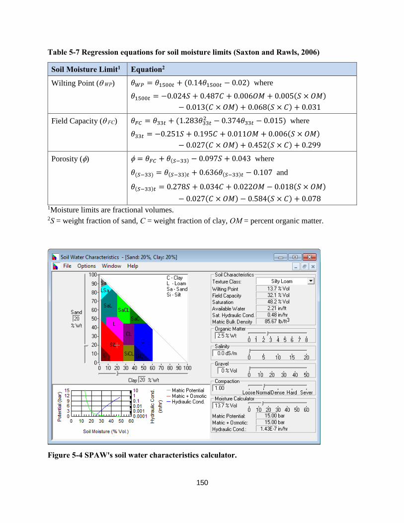
150

Table 5-7 Regression equations for soil moisture limits (Saxton and Rawls, 2006)

Soil Moisture Limit1 Equation2

Wilting Point (θ WP) 𝜃𝜃𝑊𝑊𝑃𝑃 = 𝜃𝜃1500𝑡𝑡 + (0.14𝜃𝜃1500𝑡𝑡 − 0.02) where

𝜃𝜃1500𝑡𝑡 = −0.024𝑆𝑆 + 0.487𝐶𝐶 + 0.006𝑂𝑂𝑆𝑆 + 0.005(𝑆𝑆 × 𝑂𝑂𝑆𝑆)− 0.013(𝐶𝐶 × 𝑂𝑂𝑆𝑆) + 0.068(𝑆𝑆 × 𝐶𝐶) + 0.031

Field Capacity (θ FC) 𝜃𝜃𝐹𝐹𝐻𝐻 = 𝜃𝜃33𝑡𝑡 + (1.283𝜃𝜃33𝑡𝑡2 − 0.374𝜃𝜃33𝑡𝑡 − 0.015) where

𝜃𝜃33𝑡𝑡 = −0.251𝑆𝑆 + 0.195𝐶𝐶 + 0.011𝑂𝑂𝑆𝑆 + 0.006(𝑆𝑆 × 𝑂𝑂𝑆𝑆)− 0.027(𝐶𝐶 × 𝑂𝑂𝑆𝑆) + 0.452(𝑆𝑆 × 𝐶𝐶) + 0.299

Porosity (φ) φ = 𝜃𝜃𝐹𝐹𝐻𝐻 + 𝜃𝜃(𝑆𝑆−33) − 0.097𝑆𝑆 + 0.043 where

𝜃𝜃(𝑆𝑆−33) = 𝜃𝜃(𝑆𝑆−33)𝑡𝑡 + 0.636𝜃𝜃(𝑆𝑆−33)𝑡𝑡 − 0.107 and

𝜃𝜃(𝑆𝑆−33)𝑡𝑡 = 0.278𝑆𝑆 + 0.034𝐶𝐶 + 0.022𝑂𝑂𝑆𝑆 − 0.018(𝑆𝑆 × 𝑂𝑂𝑆𝑆)− 0.027(𝐶𝐶 × 𝑂𝑂𝑆𝑆) − 0.584(𝑆𝑆 × 𝐶𝐶) + 0.078

1Moisture limits are fractional volumes. 2S = weight fraction of sand, C = weight fraction of clay, OM = percent organic matter.

Figure 5-4 SPAW's soil water characteristics calculator.

151

Table 5-8 Regression estimates of soil moisture limits from the SPAW calculator*

Soil Type

Porosity (ft3/ft3)

Field Capacity

(ft3/ft3)

Wilting Point

(ft3/ft3)

Saturated Hydraulic

Conductivity (in/hr)

Sand 0.463 0.094 0.050 4.49

Loamy sand 0.457 0.121 0.057 3.59

Sandy loam 0.450 0.179 0.081 1.98

Loam 0.458 0.267 0.126 0.73

Silt loam 0.482 0.321 0.137 0.48

Sandy clay loam 0.432 0.283 0.183 0.31

Clay loam 0.472 0.350 0.213 0.18

Silty clay loam 0.510 0.379 0.210 0.23

Sandy clay 0.440 0.371 0.260 0.03

Silty clay 0.532 0.416 0.278 0.15

Clay 0.488 0.420 0.299 0.03 *For 2.5% organic matter content by weight.

5.5.2 Percolation Parameters The two parameters that govern the percolation rate between the upper and lower groundwater zones are the soil’s saturated hydraulic conductivity KS and the coefficient HCO that characterizes the exponential decrease in hydraulic conductivity with decreasing moisture content. The most accurate way of estimating these parameters is from laboratory tests that measure hydraulic conductivity K as a function of soil moisture content θ for the particular soil under consideration. Such data for three particular soils – sand, sandy loam, and silty loam – are shown in Figure 5-5. They were generated from disturbed soil samples under desaturation (draining) conditions (see Brooks and Corey (1964) and Laliberte et al. (1966)). In some cases (e.g., sand), K(θ) may range through several orders of magnitude. Soils data of this type are becoming more readily available; for example, soil science departments at universities often publish such information (e.g., Carlisle et al., 1981).

152

Figure 5-5 Measured hydraulic conductivity for three soils.

When soil data like this are available, KS and HCO can be estimated by fitting Equation 5-20 to the data, i.e., fitting a straight line to the plot of the logarithm of K versus θ. The fits are not

153

optimal over the entire data range because the fit is only performed for the high moisture content region between field capacity and porosity. When laboratory data are not available general estimates of KS based on soil texture class can be obtained from Tables 5-3, 5-4, and 5-5. Another alternative is the regression equation derived by Saxton and Rawls (2006) from the same soils data base used to derive the moisture limit equations listed in Table 5-7. The equation for KS (in/hr) is:

𝐾𝐾𝑠𝑠 = 76(𝜙𝜙 − 𝜃𝜃𝐹𝐹𝐻𝐻)(3−𝜆𝜆) (5-24)

where 𝜆𝜆 = 0.262𝑙𝑙𝑚𝑚 � 𝜃𝜃𝐹𝐹𝐹𝐹𝜃𝜃𝑊𝑊𝑊𝑊

� and φ = soil porosity, θFC = field capacity and θWP = the wilting point.

This equation is also included in the SPAW soil water characteristics calculator described in the previous section and shown in Figure 5-4. The estimates of KS it produces for the different soil classes are shown in Table 5-8. For the Woodburn silt loam soil in Section 5.5.1, it estimates a saturated hydraulic conductivity of 0.48 in/hr (see Figure 5-4). This value falls within the range of 0.2 - 2.0 in/hr (1.4 - 14 µm/sec) listed in the Physical Properties report of Figure 4-1. HCO can be estimated by utilizing Campbell’s theoretical power law relation (Campbell, 1974) as described in Saxton and Rawls (2006):

𝐾𝐾(𝜃𝜃) = 𝐾𝐾𝑆𝑆 �𝜃𝜃𝜙𝜙

�3+2/𝜆𝜆

(5-25)

One can then estimate a value for HCO that gives a best fit between Equation 5-19 and Equation 5-25 as θ ranges between φ and θFC. Figure 5-6 shows one such fit for the soil limits associated with the Woodburn Silt Loam discussed earlier (φ = 0.482, θFC = 0.321, and θWP = 0.137). The data points come from evaluating Equation 5-25 for a series of different moisture levels θ. The line of best fit that passes through the origin has a slope of 28.864 which would be the estimate of HCO for this soil.

154

Figure 5-6 Fitting SWMM's hydraulic conductivity equation to a power law equation.

Repeating this fitting process for the sand and clay content of the various standard soil classes under a variety of organic contents, using the SPAW calculator to estimate the associated moisture limits, produced the following regression estimate for HCO:

𝐻𝐻𝐶𝐶𝑂𝑂 = 0.48(%𝑆𝑆𝑎𝑎𝑚𝑚𝑑𝑑) + 0.85(%𝐶𝐶𝑙𝑙𝑎𝑎𝐶𝐶) R2 = 0.99 (5-26)

The resulting HCO values for the different soil classes are shown in Table 5-9. A third percolation parameter, DP, governs the rate of at which water is lost from the lower saturated zone by seepage through a confining layer into a deeper groundwater aquifer. DP essentially represents the saturated hydraulic conductivity of this confining bottom layer and will therefore typically have very low values, similar to those for compacted clay soils. If water table measurements are available, DP can also be estimated from the rate at which the water table elevation drops over a prolonged dry period.

155

Table 5-9 Estimated HCO for different soil types

Soil Type Percent Sand Percent Clay HCO Sand 92 5 48

Loamy sand 82 6 44

Sandy loam 65 10 40

Loam 42 18 35

Silt loam 20 20 27

Sandy clay loam 60 28 53

Clay loam 33 34 45

Silty clay loam 10 34 34

Sandy clay 52 42 61

Silty clay 7 47 43

Clay 30 50 57

5.5.3 ET Parameters The two evapotranspiration parameters used by the groundwater routine are CET, the fraction of the available evaporation apportioned to the upper unsaturated zone, and DET, the depth from the ground surface below which no lower zone ET is possible (ft). The total rate available for subsurface evaporation is the external evaporation rate supplied to the program for the current month or day (see Section 2.5) minus the rate used for surface evaporation (Equation 5-12). The CET parameter determines what fraction of this remaining evaporation rate is used in the upper subsurface zone. In general, higher CET values will be associated with looser soils, lower water table elevations, and surface vegetation with shallow root zones. The amount of ET available to the saturated lower zone is 1 – CET of the total subsurface available ET. The fraction of this amount actually utilized is proportional to the height that the water table rises above a depth DET measured from the ground surface. DET is the maximum depth from which water may be removed by evapotranspiration. Because the lower zone is saturated, ET losses reflect mainly plant transpiration. Where surface vegetation is present, DET should at least equal the expected average depth of root penetration. The influence of plant roots usually extends somewhat below the depth of root penetration because of capillary suction to the roots. The depth of capillary draw to the surface without vegetation may be 4 to 8 inches for sands, about 8 to 18 inches in silts, and in clays about 12 to 60 inches. Rooting depth is dependent on many factors --

156

species, moisture availability, maturation, soil type, and plant density. In humid areas where moisture is readily available near the surface, grasses may have rooting depths of 6 to 24 inches. In drier areas, the rooting depth is very sensitive to plant species and to the depth to which moisture is stored and may range from 6 to 48 inches. The evaporative zone depth would be somewhat greater than the rooting depth. The local Agricultural Extension Service office can provide information on characteristic rooting depths for vegetation in specific areas. Table 5-10 presents values of DET for different combinations of soil type and ground cover that were derived from unsaturated-saturated flow simulations (Shah et al., 2007).

Table 5-10 DET (in feet) for different soil types and land cover (Shah et al., 2007)

Soil Type Bare Soil Grass Forest Sand 2 5 8

Loamy Sand 2 6 9

Sandy Loam 4 8 11

Sandy clay loam 7 10 13

Sandy clay 7 10 13

Loam 9 12 15

Silty clay 11 14 17

Clay loam 13 17 20

Silt loam 14 17 20

Silt 14 17 21

Silty clay loam 15 18 21

Clay loam 20 23 27

5.5.4 Groundwater Discharge Constants The groundwater discharge constants A1, B1, A2, B2, and A3 appear in Equation 5-22 and determine the rate of groundwater exchange with a specific node in the conveyance system. The equation is repeated here for easy reference:

𝑓𝑓𝐿𝐿 = 𝐴𝐴1(𝑑𝑑𝐿𝐿 − ℎ∗)𝐵𝐵1 − 𝐴𝐴2(ℎ𝑆𝑆𝑊𝑊 − ℎ∗)𝐵𝐵2 + 𝐴𝐴3𝑑𝑑𝐿𝐿ℎ𝑆𝑆𝑊𝑊 (5-27)

157

where the heights dL, hSW, and h* are defined in Figure 5-2. Because of its general nature this equation can assume a variety of functional forms. Several specific examples will now be discussed. Linear Reservoir The saturated groundwater zone can be thought of as a storage reservoir whose lateral outflow is linearly proportional to the water table depth dL. Two cases are possible – with and without surface water interaction. Without surface water interaction, the groundwater flow rate is simply:

𝑓𝑓𝐿𝐿 = 𝐴𝐴1(𝑑𝑑𝐿𝐿 − ℎ∗) (5-28)

In terms of Equation 5-27 this implies that A1 > 0, B1 = 1, and A2 = A3 = 0. Note that the user-supplied value of A1 would be expressed as cfs/ac-ft for US units and cms/ha-m for metric units. With surface water interaction, the groundwater flow rate is proportional to the difference between the groundwater table height and the surface water height:

𝑓𝑓𝐿𝐿 = 𝐴𝐴1(𝑑𝑑𝐿𝐿 − ℎ𝑆𝑆𝑊𝑊) (5-29)

which can be achieved with A1 = A2 > 0, B1 = B2 = 1, and A3 = 0. A1 would have the same units as before (cfs/ac-ft or cms/ha-m). Because both of these cases are empirical simplifications, A1 would have to be determined through model calibration against observed groundwater table and conveyance system head measurements. Dupuit-Forcheimer Lateral Seepage Under the assumption of uniform infiltration and horizontal flow by the Dupuit-Forcheimer approximation, the relationship between water table elevation and groundwater flow rate for the configuration shown in Figure 5-7 is (Bouwer, 1978, p.51):

𝑓𝑓𝐿𝐿 =𝐾𝐾𝑆𝑆

2𝐿𝐿2 (ℎ12 − ℎ2

2) (5-30)

where KS is the saturated hydraulic conductivity and the other parameters are defined in Figure 5-7. While h2 is the same as the surface water height hSW, h1 is the maximum groundwater table height. The height dL that SWMM computes is only an average over the catchment. One can, however, assume this average is equivalent to the average of h1 and h2, i.e.:

158

𝑑𝑑𝐿𝐿 =ℎ1 + ℎ2

2 (5-31)

so that ℎ1 = 2𝑑𝑑𝐿𝐿 − ℎ2. Substituting this and ℎ2 = ℎ𝑆𝑆𝑊𝑊 into Equation 5-30 and simplifying terms results in:

Figure 5-7 Definition sketch for Dupuit-Forcheimer seepage to an adjacent channel.

𝑓𝑓𝐿𝐿 = �2𝐾𝐾𝑆𝑆

𝐿𝐿2 � 𝑑𝑑𝐿𝐿2 − �

2𝐾𝐾𝑆𝑆

𝐿𝐿2 � 𝑑𝑑𝐿𝐿ℎ𝑆𝑆𝑊𝑊 (5-32)

Comparing Equation 5-32 with Equation 5-27 shows that the two will be equivalent if A1 = -A3 = 2KS / L2, A2 = 0, B1 = 2, and h* = 0. Note that Equation 5-30 is only valid for unidirectional flow into the receiving node, but because A3 ≠ 0, SWMM will set fG to 0 should dL drop below hSW. Hooghoudt’s Equation for Tile Drainage The geometry of a tile drainage installation is illustrated in Figure 5-8. Hooghoudt’s relationship (Bouwer, 1978, p. 295) among the indicated parameters is

𝑓𝑓𝐿𝐿 = (2𝐷𝐷𝑒𝑒 + 𝑚𝑚)4𝐾𝐾𝑆𝑆 𝑚𝑚 𝐿𝐿2⁄ (5-33)

159

where De = effective depth of the impermeable layer below the drain center, and the other parameters are defined in Figure 5-8. De is less than or equal to b0 in Figure 5-8 and is a function of b0, drain diameter, and drain spacing L; the complicated relationship is given by Bear (1972, p. 412) and graphed by Bouwer (1978, p. 296).

Figure 5-8 Definition sketch for Hooghoudt’s method for flow to circular drains.

From Figure 5-8, the maximum rise of the water table, m, is:

𝑚𝑚 = ℎ1 − 𝑏𝑏0 (5-34)

Once again approximating the average water table depth above the impermeable layer by:

𝑑𝑑𝐿𝐿 =ℎ1 + 𝑏𝑏0

2 (5-35)

results in:

𝑚𝑚 = 2(𝑑𝑑𝐿𝐿 − 𝑏𝑏0) (5-36)

Substituting 5-36 into 5-33 gives:

𝑓𝑓𝐿𝐿 = �16𝐾𝐾𝑆𝑆

𝐿𝐿2 � [(𝑑𝑑𝐿𝐿 − 𝑏𝑏0)2 − 𝐷𝐷𝑒𝑒𝑏𝑏0 + 𝐷𝐷𝑒𝑒𝑑𝑑𝐿𝐿] (5-37)

160

This can be written in a format compatible with the general groundwater discharge equation 5-27 as follows:

𝑓𝑓𝐿𝐿 = 𝐴𝐴1(𝑑𝑑𝐿𝐿 − ℎ∗)2 − 𝐴𝐴2 + 𝐴𝐴3𝑑𝑑𝐿𝐿ℎ𝑆𝑆𝑊𝑊 (5-38)

where 𝐴𝐴1 = 16𝐾𝐾𝑆𝑆/𝐿𝐿2,

𝐵𝐵1 = 2,

𝐴𝐴2 = 𝐴𝐴1𝐷𝐷𝑒𝑒𝑏𝑏0,

𝐵𝐵2 = 0,

𝐴𝐴3 = 𝐴𝐴1(𝐷𝐷𝑒𝑒 𝑏𝑏0⁄ ),

h* is set equal to b0 and a constant value of hSW only slightly higher than b0 is used. The internal units of both A1 and A3 are (ft-s)-1 while A2 has units of ft/s. In terms of the program input though, where fG is expressed as flow per acre (or per hectare), the units on A1 and A3 would be would be ft/s/ac (or m/s/ha) and for A2 would be ft3/s/ac (or m3/s/ha). Since A3 ≠ 0, flow back into the groundwater zone would not be allowed should dL drop below b0. The mathematics of drainage to ditches or circular drains is complex; several alternative formulations are described by van Schilfgaarde (1974).

5.6 Numerical Example

A simple numerical example will help illustrate the effect that groundwater can have on the runoff generated from a subcatchment. It is a variation of the runoff example used in Section 3.10 which consists of a single relatively flat, completely pervious subcatchment containing a well-drained Group B soil that is subjected to a 2-inch, 6-hour rain event. The subsurface zone beneath the subcatchment extends to a depth of 6 feet and its initial water table height is 3.5 feet. Because a conveyance node is required to complete a groundwater model, a single such node is included that receives both the surface runoff and the groundwater flow from the subcatchment. Its invert elevation is 0.5 feet above the initial water table level. The Linear Reservoir form of the groundwater discharge equation without surface water interaction is used. Table 5-11 summarizes the pertinent parameters for this example. The initial moisture content of the unsaturated zone is 0.4, midway between fully saturated and fully drained.

161

Table 5-11 Parameters used in groundwater example

Item Parameter Value Subcatchment Percent Impervious 0

Percent Slope 0.5 Width (ft) 140 Roughness 0.1 Depression Storage (in) 0.05

Rainfall Event Duration (hr) 6.0 Total Depth (in) 2.0 Time-to-Peak / Duration 0.375 Evaporation Rate (in/hr) 0.0

Horton Infiltration Initial Capacity (in/hr) 1.2 Ultimate Capacity (in/hr) 0.1 Decay Coefficient (hr-1) 2.0

Groundwater Porosity 0.5 Field Capacity 0.3 Wilting Point 0.15 Saturated Hydraulic Conductivity (in/hr) 0.1 Conductivity Curve Parameter (HCO) 12.0 Deep Percolation Constant (DP) 0.002 Reference Depth (h*) (ft) 4.0 GW Flow Coefficient (A1) (cfs/ac-ft) 0.5 GW Flow Exponent (B1) 1.0 A2, A3 and B2 0.0

The surface runoff and the groundwater flow seen by the outlet node over a 24-hour simulation period are shown in Figure 5-9. The surface runoff is unaffected by inclusion of the subsurface zones, since the upper zone never fully saturates. Its hydrograph looks the same as for the example in Section 3.10 (see the pervious curve in Figure 3-12). However, as the infiltrated water percolates through the upper soil zone, the depth of the lower saturated zone rises and begins to produce groundwater outflow into the receiving node. This outflow continues long after the surface runoff ceases, creating an extended recession limb on the total outflow hydrograph.

162

0

0.1

0.2

0.3

0.4

0.5

0.6

0.7

0 4 8 12 16 20 24

Rain

fall

or F

low

(in/

hr)

Time (hours)

Rainfall Surface Runoff Groundwater Flow Total Outflow

Figure 5-9 Surface runoff and groundwater flow for the illustrative groundwater example.

163

Chapter 6 – Snowmelt

6.1 Introduction

Snowmelt is an additional mechanism by which urban runoff may be generated. Although flow rates are typically low, they may be sustained over several days and remove a significant fraction of pollutants deposited during the winter. Rainfall events superimposed upon snowmelt baseflow may produce higher runoff peaks and volumes as well as add to the melt rate of the snow. In the context of long term continuous simulation, runoff and pollutant loads are distributed quite differently in time between the cases when snowmelt is and is not simulated. The water and pollutant storage that occurs during winter months in colder climates cannot be simulated without including snowmelt. As part of a broad program of testing and adaptation to Canadian conditions, a snowmelt routine was placed in SWMM for single event simulation by Proctor and Redfern, Ltd. and James F. MacLaren, Ltd., abbreviated PR-JFM (1976a, 1976b, 1977), during 1974-1976. The basic melt computations were based on routines developed by the U.S. National Weather Service, NWS (Anderson, 1973). The current SWMM implementation utilizes the Canadian SWMM snowmelt routines as a starting point and extends their capabilities to model long term continuous simulations. In addition, features were added to adapt the snowmelt process to urban conditions, since the snowmelt routines used in other watershed runoff models are aimed primarily at simulation of spring melts in large river basins. The work of the National Weather Service (Anderson, 1973, 2006) as reflected in their SNOW-17 model was heavily utilized, especially for the extension to continuous simulation and the resulting inclusion of cold content, variable melt coefficients, and areal depletion. Several hydrologic models include snowmelt computations, e.g., Stanford Watershed Model (Crawford and Linsley, 1966), HSPF (Bicknell et al., 1997), NWS (Anderson, 1973, 1976), STORM (Corps of Engineers, 1977; Roesner et al., 1974), SSARR (Corps of Engineers, 1971), and PRMS (Leavesley et al., 1983). Useful summaries of snowmelt modeling techniques are available in texts by Eagleson (1970), Gray (1970), Fleming (1975), Linsley et al. (1975), Bedient et al. (2013), and Viessman and Lewis (2003). All of these draw upon the classic work, Snow Hydrology, of the Corps of Engineers (1956). A review of snowmelt components of urban drainage models has been performed by Semádeni-Davies (2000). Three models were reviewed in some detail: SWMM (version 4), MouseNAM (Danish Hydraulic Institute, 1994), and HBV (Bergström, 1976; Lindström et al., 1997). Semádeni-Davies (2000) concludes that urban snowmelt routines (including those in SWMM)

164

have been adapted directly from models developed for rural situations and therefore may not represent urban conditions well. Degree-day methods are used in all three models that she reviewed, and only limited information is available regarding coefficients in urban areas. Plowing and piling of snow in urban areas, and the change in the nature of its albedo and density are also important considerations, for which SWMM includes options for their representation. Overall, SWMM appears to be no better – and no worse – than the other two models reviewed. The descriptions of SWMM snowmelt algorithms that follow do not reflect any general improvements recommended by Semádeni-Davies (2000).

6.2 Preliminaries

6.2.1 Snow Depth SWMM treats all snow depths as “depth of water equivalent” to avoid specification of the specific gravity of the snow pack, which is highly variable with time. The specific gravity of new snow is of the order of 0.09; an 11:1 or 10:1 ratio of snow pack depth to water equivalent depth is often used as a rule of thumb. With time, the pack compresses until the specific gravity can be considerably greater, to 0.5 and above. In urban areas, lingering snow piles may resemble ice more than snow with specific gravities approaching 1.0. Although snow pack heat conduction and storage depend on specific gravity, sufficient accuracy may be obtained without involving specific gravity. It is adequate to maintain continuity through the use of depth of water equivalent. Most input parameters are in units of inches or mm of water equivalent (in w.e., or mm w.e.). For all internal computations, conversions are made to feet of water equivalent.

6.2.2 Meteorological Inputs Snowfall rates are determined directly from precipitation inputs by using a dividing temperature SNOTMP. If the current air temperature is at or below SNOTMP, the precipitation falls as snow. Otherwise it falls as rain. In natural areas, a surface temperature of 34° to 35°F (1-2°C) provides the dividing line between equal probabilities of rain and snow (Eagleson, 1970; Corps of Engineers, 1956). However, this separation temperature might need to be somewhat lower in urban areas due to warmer surface temperatures. Precipitation gages tend to produce inaccurate snowfall measurements because of the complicated aerodynamics of snowflakes falling into the gage. Snowfall totals are generally underestimated as a result, by a factor that varies considerably depending upon gage exposure, wind velocity and whether or not the gage has a wind shield. The program includes a multiplier for each Rain gage

165

object, the Snow Catch Factor (SCF), which adjusts for these effects. The SCF is only applied when precipitation falls as snow. Although it will vary considerably from storm to storm, SCF acts as a mean correction factor over a season in the model. Anderson (1973) provides typical values of SCF as a function of wind speed, as shown in Figure 6-1, which may be helpful in establishing an initial estimate. The value of SCF can also be used to account for other factors, such as losses of snow due to interception and sublimation not accounted for in the model. Anderson (1973) states that both losses are usually small compared to the gage catch deficiency. As discussed in Section 2.3, air temperature data is supplied to a SWMM data set from either a user-generated time series or from a climate file. If a time series is used, the entries represent instantaneous temperature readings at given points in time. Linear interpolation is used to obtain temperature values for times that fall in between those recorded in the time series. If a climate file is used, then a continuous record of maximum and minimum daily temperatures is provided. The sinusoidal interpolation method described in Section 2.4 is used to obtain an instantaneous value at any point in time during a day based on the day’s max-min values. (Any missing days in the record are filled in with the max-min values from the previous day). During the simulation, melt is generated at each time step using a degree-day type equation during dry weather and a heat balance equation during rainfall periods. The latter equation makes an adjustment for wind speed (higher melt rates at higher wind speeds). The input of wind speed data to the program was discussed in Section 2.4. There are two options: 1) as average values for each month of the year, or 2) as daily values from the same climate file used to supply daily max-min temperatures. Should wind speed data not be available, the adjustment to the melt equation is simply ignored. The coefficients used in the degree-day melt equation vary sinusoidally, from a maximum on June 21 to a minimum on December 21. In addition, a record of the cold content of the snow is maintained. Thus, before melt can occur, the pack must be “ripened,” that is, heated to a specified base temperature. Specified, constant areas of each subcatchment may be designated as snow covered, or, following the practice of melt computations in natural basins, “areal depletion curves” may be used to describe the spatial extent of snow cover as the pack melts. For instance, shaded areas would be expected to retain a snow cover longer than exposed areas. Thus, the snow covered area of each subcatchment changes with time during the simulation. Melt, after routing through the remaining snow pack, is combined with rainfall to form the spatially weighted “effective rainfall” for overland flow routing.

166

Figure 6-1 Typical gage catch deficiency correction (Anderson, 2006, p. 8).

6.2.3 Subcatchment Partitioning Just as it was convenient to partition a subcatchment into three distinct areas for computing runoff (a pervious area and impervious areas both with and without depression storage – see Section 3.2), the same is true for snowmelt. The partitioning is made to facilitate the modeling of both snow removal (i.e. plowing) operations and the areal depletion phenomenon. It uses the same fractions of pervious and total impervious areas as for runoff, but instead of dividing the impervious area on the presence or absence of depression storage, it does so based on snow removal capability. That is, one fraction of the impervious area can be subjected to snow removal but not areal depletion while the reverse is true for the remaining fraction. Streets, sidewalks, and parking lots would fall into the first category, which can be considered almost normally bare of snow. Rooftops would better fit the second. Figure 6-2 illustrates the subcatchment partitioning used for snowmelt and compares it with the one used for runoff.

167

SA1

SA3

SA2 A1

A2 A3

Snowmelt Sub-Areas: SA1 = pervious SA2 = plowable impervious SA3 = remaining impervious

Runoff Sub-Areas: A1 = pervious (= SA1) A2 = impervious w/ depression storage A3 = impervious w/o depression storage

Figure 6-2 Subcatchment partitionings used for snowmelt and runoff.

A separate accounting is kept for snow accumulation and melting from each of these fractions (pervious, plowable impervious, and remaining impervious). After snowmelt calculations are made at the start of each time step, the net precipitation over the plowable and remaining impervious areas are summed together and then, for the purpose of computing runoff, are re-distributed between the fractions of impervious areas with and without depression storage. Because the pervious areas for runoff and snowmelt are the same, the snowmelt result over this sub-area can be used directly for computing pervious area runoff.

168

6.2.4 Redistribution and Snow Removal Snow removal practices form a major difference between the snow hydrology of urban and rural areas. Much of the snow cover may be completely removed from heavily urbanized areas, or plowed into windrows or piles, with melt characteristics that differ markedly from those of undisturbed snow. Management practices in cities vary according to location, climate, topography and the storm itself; they are summarized in Table 6.1. It is probably not possible to treat them all in a simulation model. However, provision is made to simulate approximately some of these practices.

6.2.5 Effect on Infiltration A snow pack tends to insulate the surface beneath it. If ground has frozen prior to snowfall, it will tend to remain so, even as the snow begins to melt. Conversely, unfrozen ground is generally not frozen by subsequent snowfall. The infiltration characteristics of frozen versus unfrozen ground are not well understood and depend upon the moisture content at the time of freezing. For these and other reasons, SWMM assumes that snow has no effect on infiltration or other parameters, such as surface roughness or detention storage (although the latter is altered in a sense through the use of the free water holding capacity of the snow). In addition, all heat transfer calculations cease when the water becomes “net runoff”. Thus, water in temporary surface storage during the overland flow routing will not refreeze as the temperature drops and is also subject to evaporation beneath the snow pack. It is assumed that all snow subject to “redistribution”, (e.g., plowing) resides on a user-specified fraction of the total impervious area (area SA2 in Figure 6-2) that might consist of streets, sidewalks, parking lots, etc. (The desired degree of definition may be obtained by using several subcatchments, although a coarse schematization, e.g., one or two subcatchments, may be sufficient for some continuous simulations.) The following five parameters, which can vary by subcatchment, govern how snow is removed or re-distributed from this sub-area:

Fimp: fraction of current snow transferred to the remaining impervious sub-area (SA3)

Fperv: fraction of current snow transferred to the pervious area (SA1)

Fsub: fraction of current snow transferred to the pervious area of another designated subcatchment.

Fout: fraction of current snow transferred out of the watershed

Fimelt: fraction of current snow converted into immediate melt

169

An instantaneous redistribution of the current snow depth begins when the latter exceeds the user-supplied parameter WEPLOW. Fimp or Fperv are used if snow is usually windrowed onto adjacent impervious or pervious areas. If it is trucked to the pervious area of another subcatchment, the fraction Fsub will so indicate, or Fout can be used if the snow is removed entirely from the simulated watershed. In the latter case, such removals are tabulated and included in the final continuity check. Finally, excess snow may be immediately “melted” (i.e., treated as rainfall), using Fimelt. The five fractions can sum to less than 1.0 in which case some residual snow will remain on the surface. See Table 6-1 for guidelines on typical levels of service for snow and ice control (Richardson et al., 1974). The snow redistribution process does not account for snow management practices that use chemicals, such as roadway salting. This is handled using the melt equations, as described subsequently. No pollutants are transferred with the snow. The transfers listed above are assumed to have no effect on pollutant washoff and regeneration. In addition, all the redistribution parameters remain constant throughout the simulation and can only represent averages over a snow season.

6.3 Governing Equations

6.3.1 Overview Excellent descriptions of the processes of snowmelt and accumulation are available in several texts and simulation model reports and in the well-known 1956 Snow Hydrology report by the Corps of Engineers. The important heat budget and melt components are mentioned briefly here; any of the above sources may be consulted for detailed explanations. A brief justification for the techniques adopted for snowmelt calculations in SWMM is presented below.

170

Table 6-1 Guidelines for level of service in snow and ice control (Richardson et al., 1974)

Road Classification Level of Service

Snow Depth to Start Plowing (Inches)

Max. Snow Depth on Pavement (Inches)

Full Pavement Clear of Snow After Storm (Hours)

Full Pavement Clear of Ice After Storm (Hours)

Low-Speed Multilane Urban Expressway

Roadway routinely patrolled during storms All traffic lanes treated with chemicals All lanes (including breakdown lanes) operable at all times but at reduced speeds Occasional patches of well sanded snow pack Roadway repeatedly cleared by echelons of plows to minimize traffic disruption Clear pavement obtained as soon as possible

0.5 to 1 1 1 12

High Speed 4-Lane Divided Highways; Interstate System; ADT greater than 10,000a

Roadway routinely patrolled during storms Driving and passing lanes treated with chemicals Driving lane operable at all times at reduced speeds Passing lane operable depending on equipment availability Clear pavement obtained as soon as possible

1 2 1.5 12

Primary Highways; Undivided 2 and 3 lanes; ADT 500-5000a

Roadway is routinely patrolled during storms Mostly clear pavement after storm stops Hazardous areas receive treatment of chemicals or abrasive Remaining snow and ice removed when thawing occurs

1 2.5 2 24

Secondary Roads ADT less than 500a

Roadway is patrolled at least once during a storm Bare left-wheel track with intermittent snow cover Hazardous areas are plowed and treated with chemicals or abrasives as a first order of work Full width of road is cleared as equipment becomes available

2 3 3 48

aADT – average daily traffic Snowpack Heat Budget

171

Heat may be added or removed from a snowpack by the following processes:

• Absorbed solar radiation (addition). • Net long wave radiation exchange with the surrounding environment (addition or removal). • Convective (diffusive) transfer of sensible heat from/to air (addition or removal). • Release of latent heat of vaporization by condensate (addition) or, the opposite, its removal

by sublimation (removing the latent heat of vaporization plus the latent heat of fusion). • Advection of heat by rain (addition) plus addition of the heat of fusion if the rain freezes. • Conduction of heat from underlying ground (removal or addition).

The terms may be summed, with appropriate signs, and equated to the change of heat stored in the snowpack to form a conservation of heat equation. All of the processes listed above vary in relative importance with topography, season, climate, local meteorological conditions, etc., but items 1-4 are the most important. Item 5 is of less importance on a seasonal basis, and item 6 is often neglected. A snow pack is termed “ripe” when any additional heat will produce liquid runoff. Rainfall (item 5) will rapidly ripen a snowpack by release of its latent heat of fusion as it freezes in subfreezing snow, followed by quickly filling the free water holding capacity of the snow. Melt Prediction Techniques Prediction of melt follows from prediction of the heat storage of the snow pack. Energy budget techniques are the most exact formulation since they evaluate each of the heat budget terms individually, requiring as meteorological input quantities such as solar radiation, air temperature, dew point or relative humidity, wind speed, and precipitation. Assumptions must be made about the density, surface roughness and heat and water storage (mass balance) of the snow pack as well as on related topographical and vegetative parameters. Further complications arise in dealing with heat conduction and roughness of the underlying ground and whether or not it is permeable. Several models treat some or all of these effects individually, for instance, the NWS river forecast system developed by Anderson (1976). Interestingly, under many conditions he found that results obtained using his energy balance model were not significantly better than those obtained using simpler (e.g., degree-day or temperature-index) techniques in his earlier model (Anderson, 1973). The more open and variable the condition, the better is the energy balance technique. Closest agreement between his two models was for heavily forested watersheds. The minimal data needed to apply an energy balance model are a good estimate of incoming solar radiation, plus measurements of air temperature, vapor pressure (or dew point or relative humidity) and wind speed. All of these data, except possibly solar radiation, are available for at least one location (e.g., the airport) for almost all reasonably sized cities. Even solar radiation measurements

172

are taken at several locations in most states. Predictive techniques are also available, for solar radiation and other parameters, based on available measurements (TVA, 1972; Franz, 1974). Choice of Predictive Method Two major reasons suggest that simpler, e.g., temperature-index, techniques should be used for simulation of snowmelt and accumulation in urban areas. First, even though required meteorological data for energy balance models are likely to be available, there is a large local variation in the magnitude of these parameters due to the urbanization itself. For example, radiation melt will be influenced heavily by shading of buildings and albedo (reflection coefficient) reduced by urban pollutants. In view of the many unknown properties of the snowpack itself in urban areas, it may be overly ambitious to attempt to predict melt at all! But at the least, simpler techniques are probably all that are warranted. They have the added advantage of considerably reducing the already extensive input data to a model such as SWMM. Second, the objective of the modeling should be examined. Although it may contribute, snowmelt seldom causes flooding or hydrologic extremes in an urban area itself. Hence, exact prediction of flow magnitudes does not assume nearly the importance it has in the models of, say, the NWS, in which river flood forecasting for large mountainous catchments is of paramount importance. For planning purposes in urban areas, exact quantity (or quality) prediction is not the objective in any event; rather, these efforts produce a statistical evaluation of a complex system and help identify critical time periods for more detailed analysis. For these and other reasons, simple snowmelt prediction techniques are incorporated into SWMM. Anderson’s NWS (1973) temperature-index method is also well documented and tested, and is used in SWMM. As described subsequently, the snowmelt modeling follows Anderson’s work in several areas, not just in the melt equations. It may be noted that the STORM model (Corps of Engineers, 1977; Roesner et al., 1974) also uses the temperature-index method for snowmelt prediction, in a considerably less complex manner than is programmed in SWMM.

6.3.2 Melt Equations Anderson’s NWS model (1973) treats two different melt situations: with and without rainfall. When there is rainfall (greater than 0.1 in/hr or 2.5 mm/hr in the NWS model, (greater than 0.02 in/hr or 0.51 mm/hr in SWMM), accurate assumptions can be made about several energy budget terms. These are: zero solar radiation, incoming long wave radiation equals blackbody radiation at the ambient air temperature, the snow surface temperature is 32° F (0° C), and the dew point and

173

rain water temperatures equal the ambient air temperature. Anderson combines the appropriate terms for each heat budget component into one equation for the melt rate SMELT:

𝑆𝑆𝑆𝑆𝐸𝐸𝐿𝐿𝑇𝑇 = (0.001167 + 7.5𝛾𝛾𝑈𝑈𝐴𝐴 + 0.007𝑚𝑚)(𝑇𝑇𝑚𝑚 − 32) + 8.5𝑈𝑈𝐴𝐴(𝑚𝑚𝑚𝑚

− 0.18) (6-1)

where SMELT = melt rate (in/hr) Ta = air temperature (° F) γ = psychrometric constant (in Hg/° F) UA = wind speed adjustment factor (in/in Hg – hr) i = rainfall intensity (in/hr) ea = saturation vapor pressure at air temperature (in Hg).

The origin of the numerical constants found in Equation 6-1 is given by Anderson (1973), and reflect units conversions as well as U.S. customary units for physical properties. The psychrometric constant, γ, is calculated as:

𝛾𝛾 = 0.000359𝑃𝑃𝑚𝑚 (6-2)

where Pa is the atmospheric pressure (in Hg). The latter, in turn, is calculated as a function of elevation, z:

𝑃𝑃𝑚𝑚 = 29.9 − 1.02(𝑑𝑑 1000) + 0.0032(𝑑𝑑 1000)⁄ 2.4⁄ (6-3)

where z is the average catchment elevation (ft). The wind adjustment factor, UA, accounts for turbulent transport of sensible heat and water vapor. Anderson (1973) gives:

𝑈𝑈𝐴𝐴 = 0.006𝑈𝑈 (6-4) where U is the average wind speed 1.64 ft (0.5 m) above the snow surface (mi/hr). In practice, available wind data are used and are seldom corrected for the actual elevation of the anemometer. Section 6.2.2 (as well as Section 2.6) discusses how wind data are supplied to SWMM. If no such data are available on a particular date then UA is set equal to 0. Finally, the saturation vapor pressure, ea, is given accurately by the convenient exponential approximation:

𝑚𝑚𝑚𝑚 = 8.1175 × 106𝑚𝑚𝑚𝑚𝑒𝑒 �−7701.544

𝑇𝑇𝑚𝑚 + 405.0265� (6-5)

174

During non-rain periods, melt is calculated as a linear function of the difference between the air temperature, Ta, and a base temperature, Tbase, using a degree-day or temperature-index type equation:

𝑆𝑆𝑆𝑆𝐸𝐸𝐿𝐿𝑇𝑇 = 𝐷𝐷𝐻𝐻𝑆𝑆(𝑇𝑇𝑚𝑚 − 𝑇𝑇𝑏𝑏𝑎𝑎𝑐𝑐𝑚𝑚) (6-6)

where: SMELT = melt rate (in/hr), Ta = air temperature (° F) Tbase = base melt temperature (° F) DHM = melt coefficient (in/hr-° F)

Different values of Tbase and DHM may be used for each of the three types of snow surfaces within a subcatchment. For instance, these parameters may be used to account for street salting, which lowers the base melt temperature. If desired, rooftops could be simulated using a lower value of Tbase to reflect heat transfer vertically through the roof. Suggested values for Tbase and DHM are provided in the Parameter Estimates section (6.7) below. During the simulation, Tbase remains constant, but DHM is allowed a seasonal variation, as illustrated in Figure 6-3. Following Anderson (1973), the minimum melt coefficient is assumed to occur on December 21 and the maximum on June 21. Parameters DHMIN and DHMAX are supplied as input for the three snowpack areas of each subcatchment, and sinusoidal interpolation is used to produce a value of DHM that is constant over each day of the year:

𝐷𝐷𝐻𝐻𝑆𝑆 = �𝐷𝐷𝐻𝐻𝑆𝑆𝐴𝐴𝑋𝑋 + 𝐷𝐷𝐻𝐻𝑆𝑆𝐼𝐼𝐶𝐶

2� + �

𝐷𝐷𝐻𝐻𝑆𝑆𝐴𝐴𝑋𝑋 − 𝐷𝐷𝐻𝐻𝑆𝑆𝐼𝐼𝐶𝐶2

� 𝑐𝑐𝑚𝑚𝑚𝑚 �𝜋𝜋

182(𝑑𝑑𝑎𝑎𝐶𝐶 − 81)�

(6-7)

where DHMIN = minimum melt coefficient, occurring Dec. 21 (in/hr-°F) DHMAX = maximum melt coefficient, occurring June 21 (in/hr-°F) day = number of the day of the year.

No special allowance is made for leap year. However, the correct date (and day number) is maintained.

175

Figure 6-3 Seasonal variation of melt coefficients.

6.3.3 Snow Pack Heat Exchange During subfreezing weather, the snow pack does not melt, and heat exchange with the atmosphere can either warm or cool the pack. The difference between the heat content of the subfreezing pack and the (higher) base melt temperature is taken as positive and termed the “cold content” of the pack. No melt will occur until the cold content is reduced to zero. It is maintained in inches (or feet) of water equivalent. That is, a cold content of 0.1 in. (2.5 mm) is equivalent to the heat required to melt 0.1 in. (2.5 mm) of snow. Following Anderson (1973), the heat exchange altering the cold content within each 6-hour period is proportional to the difference between the air temperature, Ta, and an antecedent temperature index, ATI, indicative of the temperature of the surface layer of the snow pack. The value of ATI is updated at the start of each time step as follows:

𝐴𝐴𝑇𝑇𝐼𝐼 ← 𝐴𝐴𝑇𝑇𝐼𝐼 + 𝑇𝑇𝐼𝐼𝑃𝑃𝑆𝑆𝑡𝑡(𝑇𝑇𝑚𝑚 − 𝐴𝐴𝑇𝑇𝐼𝐼) (6-8)

where TIPMt is given by (Anderson, 2006):

𝑇𝑇𝐼𝐼𝑃𝑃𝑆𝑆𝑡𝑡 = 1 − (1 − 𝑇𝑇𝐼𝐼𝑃𝑃𝑆𝑆)∆𝑡𝑡/6 (6-9)

for a time step ∆t in hours. TIPM is a 6-hour weighting factor whose value lies between 0 and 1.0. The value of ATI is not allowed to exceed Tbase, and when snowfall is occurring, ATI takes on the current air temperature.

176

The weighting factor TIPM is a user-supplied constant that applies over the entire watershed. It is an indication of the thickness of the “surface” layer of snow. Values less than 0.1 give significant weight to temperatures over the past week or more and would thus indicate a deeper layer than values greater than, say, 0.5, which would essentially only give weight to temperatures during the past day. In other words, the pack will both warm and cool more slowly with low values of TIPM. Anderson states that TIPM = 0.5 has given reasonable results in natural watersheds, although there is some evidence that a lower value may be more appropriate. No calibration has been attempted on urban watersheds. After the antecedent temperature index is calculated, the cold content COLDC is changed by an amount

∆𝐶𝐶𝐶𝐶 = 𝑅𝑅𝐶𝐶𝑆𝑆 × 𝐷𝐷𝐻𝐻𝑆𝑆 × (𝐴𝐴𝑇𝑇𝐼𝐼 − 𝑇𝑇𝑚𝑚) × ∆𝑚𝑚 (6-10)

where ∆CC = change in cold content (inches water equivalent) RNM = ratio of negative melt coefficient to melt coefficient, DHM = melt coefficient (in/hr-° F) ATI = antecedent temperature index (°F) Δt = time step (hr).

Note that the cold content is increased, (∆CC is positive) when the air temperature is less (colder) than the antecedent temperature index. Since heat transfer during non-melt periods is less than during melt periods, Anderson uses a “negative melt coefficient” in the heat exchange computation. SWMM computes this simply as a fraction, RNM, of the melt coefficient, DHM. Hence, the negative melt coefficient, i.e., the product DHMRNM × also varies seasonally. As with TIPM, a single user-supplied value of RNM is used throughout the study area. A typical value is 0.6. During melting periods, cold content of the pack is reduced by an amount:

∆𝐶𝐶𝐶𝐶 = −𝑆𝑆𝑆𝑆𝐸𝐸𝐿𝐿𝑇𝑇 × 𝑅𝑅𝐶𝐶𝑆𝑆 × ∆𝑚𝑚 (6-11)

with an equal reduction made in SMELT. Thus no liquid melt actually occurs until the snow pack cold content is reduced to 0. Even then, runoff will not occur, until the “free water holding capacity” of the snow pack is filled. This is discussed subsequently. The value of COLDC is in units of inches of water equivalent over the area in question. The cold content “volume,” equivalent to calories or BTUs, is obtained by multiplying by the area. Finally, an adjustment is made to Equations 6-10 and 6-11 depending on the areal extent of snow cover. This is discussed below.

177

6.4 Areal Depletion The snow pack on a catchment rarely melts uniformly over the total area. Rather, due to shading, drifting, topography, etc., certain portions of the catchment will become bare before others, and only a fraction, ASC, will be snow covered. This fraction must be known in order to compute the snow covered area available for heat exchange and melt, and to know how much rain falls on bare ground. Because of year to year similarities in topography, vegetation, drift patterns, etc., the fraction, ASC, is primarily a function of the amount of snow on the catchment at a given time; this function, called an “areal depletion curve”, is discussed below. These functions are used as an option to describe the seasonal growth and recession of the snow pack. For short, single event simulation, fractions of snow covered area may be fixed for the pervious and impervious areas of each subcatchment. As used in most snowmelt models, it is assumed that there is a depth, SI, above which there will always be 100 percent cover. In some models, the value of SI is adjusted during the simulation; in SWMM it remains constant. The amount of snow present at any time is indicated by the state variable WSNOW, which is the depth (water equivalent) over each of the three possible snow covered areas of each subcatchment (see Figure 6-2). This depth is made non-dimensional by dividing it by SI for use in calculating ASC. Thus, an areal depletion curve (ADC) is a plot of WSNOW / SI versus ASC; a typical ADC for a natural catchment is shown in Figure 6-4. For values of the ratio AWESI = WSNOW / SI greater than 1.0, ASC = 1.0, that is, the area is 100 percent snow covered.

178

Figure 6-4 Typical areal depletion curve for natural area (Anderson, 1973, p. 3-15) and temporary curve for new snow.

Some of the implications of different functional forms of the ADC may be seen in Figure 6-5. Since the program maintains snow quantities, WSNOW, as the depth over the total area, AT, the actual snow depth, WS, and actual area covered, AS, are related by continuity:

𝑊𝑊𝑆𝑆𝐶𝐶𝑂𝑂𝑊𝑊 × 𝐴𝐴𝑇𝑇 = 𝑊𝑊𝑆𝑆 × 𝐴𝐴𝑆𝑆 (6-12)

where: WSNOW = depth of snow over total area (inches water equivalent) AT = total area (ft2), WS = actual snow depth (inches water equivalent), and AS = snow covered area (ft2).

In terms of parameters shown on the ADC, this equation may be rearranged to read:

179

𝐴𝐴𝑊𝑊𝐸𝐸𝑆𝑆𝐼𝐼 = 𝑊𝑊𝑆𝑆𝐶𝐶𝑂𝑂𝑊𝑊 𝑆𝑆𝐼𝐼 = (𝑊𝑊𝑆𝑆 𝑆𝑆𝐼𝐼⁄ )(𝐴𝐴𝑆𝑆 𝐴𝐴𝑇𝑇⁄ ) = (𝑊𝑊𝑆𝑆 𝑆𝑆𝐼𝐼⁄ )𝐴𝐴𝑆𝑆𝐶𝐶⁄ (6-13) This equation can be used to compute the actual snow depth, WS, from known ADC parameters, if desired. It is unnecessary to do this in the program, but it is helpful in understanding the curves of Figure 6-5. Thus:

𝑊𝑊𝑆𝑆 = (𝐴𝐴𝑊𝑊𝐸𝐸𝑆𝑆𝐼𝐼 𝐴𝐴𝑆𝑆𝐶𝐶⁄ ) 𝑆𝑆𝐼𝐼 (6-14)

Consider the three ADC curves B, C and D of Figure 6-5. For curve B, AWESI is always less than ASC; hence WS is always less than SI as shown in Figure 6-5d. For curve C, AWESI = ASC, hence WS = SI, as shown in Figure 6-5e. Finally, for curve D, AWESI is always greater than ASC; hence, WS is always greater than SI, as shown in Figure 6-5f. Constant values of ASC at 100 percent cover and 40 percent cover are illustrated in Figure 6-5c, curve A, and Figure 6-5g, curve E, respectively. At a given time (e.g., t1 in Figure 6-5), the area of each snow depth versus area curve is the same and equal to 𝐴𝐴𝑊𝑊𝐸𝐸𝑆𝑆𝐼𝐼 × 𝑆𝑆𝐼𝐼, (e.g., 0.8 SI for time t1). Curve B on Figure 6-5a is the most common type of ADC occurring in nature, as shown in Figure 6-4. The convex curve D requires some mechanism for raising snow levels above their original depth, SI. In nature, drifting provides such a mechanism; in urban areas, plowing and windrowing could cause a similar effect. A complex curve could be generated to represent specific snow removal practices in a city. However, the program uses only one ADC curve for all impervious areas (e.g., area SA3 of Figure 6-2 for all subcatchments) and only one ADC curve for all pervious areas (e.g., area SA1 of Figure 6-2 for all subcatchments). This limitation should not hinder an adequate simulation since the effects of variations in individual locations are averaged out in the city-wide scope of most continuous simulations. The program does not require the ADC curves to pass through the origin, AWESI = ASC = 0; they may intersect the abscissa at a value of ASC > 0 in order to maintain some snow covered area up until the instant that all snow disappears (see Figure 6-4). However, the curves may not intersect the ordinate, AWESI > 0 when ASC = 0. The preceding paragraphs have centered on the situation where a depth of snow greater than or equal to SI has fallen and is melting. (The ADC curves are not employed until WSNOW becomes less than SI.) The situation when there is new snow needs to be discussed, starting from both zero and non-zero initial cover. The SWMM procedure again follows Anderson’s NWS method (1973).

180

Figure 6-5 Effect of snow cover on areal depletion curves.

When there is new snow and WSNOW is already greater than or equal to SI, ASC remains unchanged at 1.0. However, when there is new snow on bare or partially bare ground, it is assumed that the total area is 100 percent covered for a period of time, and a “temporary” ADC is established as shown in Figure 6-4. This temporary curve returns to the same point on the ADC as the snow melts. Let the depth of new snow be SNO, measured in equivalent inches of water. Then the value of AWESI will be changed from an initial value of AWE to a new value of SNEW by:

181

𝑆𝑆𝐶𝐶𝐸𝐸𝑊𝑊 = 𝐴𝐴𝑊𝑊𝐸𝐸 + 𝑆𝑆𝐶𝐶𝑂𝑂 𝑆𝑆𝐼𝐼⁄ (6-15)

It is assumed that the areal snow cover remains at 100 percent until 25 percent of the new snow melts. This defines the value of SBWS of Figure 6-4 as:

𝑆𝑆𝐵𝐵𝑊𝑊𝑆𝑆 = 𝐴𝐴𝑊𝑊𝐸𝐸 + 0.75(𝑆𝑆𝐶𝐶𝑂𝑂 𝑆𝑆𝐼𝐼⁄ ) (6-16)

Anderson (1973) reports low sensitivity of model results to the arbitrary 25 percent assumption. When melt produces a value of AWESI between SBWS and AWE, linear interpolation of the temporary curve is used to find ASC until the actual ADC curve is again reached. When new snow has fallen, the program thus maintains values of AWE, SBA and SBWS (Figure 6-4). The interactive nature of melt and fraction of snow cover is not accounted for during each time step. It is sufficient to use the value of ASC at the beginning of each time step, especially with a short (e.g., one-hour) time step for the simulation. The fraction of area that is snow covered, ASC, is used to adjust 1) the volume of melt that occurs, and 2) the “volume” of cold content change, since it is assumed that heat transfer occurs only over the snow covered area. The melt rate is computed from either of the two equations for SMELT. The snow depth is then reduced by an amount ∆WSNOW which equals:

∆𝑊𝑊𝑆𝑆𝐶𝐶𝑂𝑂𝑊𝑊 = 𝑆𝑆𝑆𝑆𝐸𝐸𝐿𝐿𝑇𝑇 × 𝐴𝐴𝑆𝑆𝐶𝐶 × ∆𝑚𝑚 (6-17) and includes appropriate continuity checks to avoid melting more snow than is there, etc. Cold content changes are also adjusted by the value of ASC. Thus, using Equation 6-10, cold content, COLDC, is changed by an amount ∆CC given by:

∆𝐶𝐶𝐶𝐶 = 𝑅𝑅𝐶𝐶𝑆𝑆 × 𝐷𝐷𝐻𝐻𝑆𝑆 × (𝐴𝐴𝑇𝑇𝐼𝐼 − 𝑇𝑇𝑚𝑚) × ∆𝑚𝑚 × 𝐴𝐴𝑆𝑆𝐶𝐶 (6-18)

where variables are as previously defined. Again there are program checks for negative values of COLDC, etc.

182

6.5 Net Runoff Production of melt does not necessarily mean that there will be liquid runoff at a given time step since a snow pack, acting as a porous medium with a “porosity,” has a certain “free water holding capacity” at a given instant in time. Conway and Benedict (1994) describe the physics of the various processes underway as melt infiltrates into a snowpack. Following PR-JFM (1976a, 1976b), this capacity is taken to be a constant fraction, FWFRAC, of the variable snow depth, WSNOW, at each time step. This volume (depth) must be filled before runoff from the snow pack occurs. The program maintains the depth of free water, FW, inches of water, for use in these computations. When WSNOWFWFRACFW ×= , the snow pack is fully ripe. The procedure is sketched in Figure 6-6.

Figure 6-6 Schematic of liquid water routing through snow pack.

183

The inclusion of the free water holding capacity via this simple reservoir-type routing delays and somewhat attenuates the appearance of liquid runoff. When rainfall occurs, it is added to the melt rate entering storage as free water. No free water is released when melt does not occur, but remains in storage, available for release when the pack is again ripe. This re-frozen free water is not included in subsequent cold content or melt computations. Melt from snow covered areas and rainfall on bare surfaces is area weighted and combined to produce net runoff onto the surface as follows:

𝑅𝑅𝐼𝐼 = 𝐴𝐴𝑆𝑆𝐶𝐶 × 𝑆𝑆𝑆𝑆𝐸𝐸𝐿𝐿𝑇𝑇 + (1.0 − 𝐴𝐴𝑆𝑆𝐶𝐶) × 𝑚𝑚 (6-19)

where RI is the net equivalent precipitation input onto the subcatchment surface (in/hr) and i is the liquid rainfall intensity (in/h). RI is used in place of the externally supplied rainfall value in subsequent overland flow and infiltration calculations. If immediate melt is produced through the use of the snow redistribution fraction Fimelt it is added to the last equation. Furthermore, all melt calculations are ended when the depth of snow water equivalent becomes less than 0.001 in. (0.025 mm), and any remaining snow and free water are converted to immediate melt and added to Equation 6-19.

6.6 Computational Scheme Snowmelt computations are a sub-procedure implemented as part of SWMM’s runoff calculations. They are made at each runoff time step, for each subcatchment that has snow pack parameters assigned to it, immediately after atmospheric precipitation has been determined. This is at Step 3a of the runoff procedure described in Section 3.4. The snowmelt routine returns an adjusted precipitation rate (in/h), consisting of liquid rainfall and/or snowmelt, over each runoff sub-area of the subcatchment. These rates serve as the actual precipitation input used in the remainder of the surface runoff computation. The steps used to compute snow accumulation and snowmelt are listed in the sidebar below.

184

Computational Scheme for Snowmelt The following variables are assumed known at the start of the time step of length ∆t (h) for each subcatchment: Externally supplied time series variables:

Ta = air temperature (°F) U = wind speed (mi/h) i = precipitation rate (in/h).

State variables for the snow pack on each snow surface:

WSNOW = snow pack depth (inches water equivalent) COLDC = cold content depth (inches water equivalent) FW = free water depth (inches water equivalent) ATI = antecedent temperature index (°F).

In addition, the following constant parameters have been supplied by the user: Constants defined for each subcatchment assigned a Snow Pack object:

SNN = fraction of impervious area that is plowable (i.e., SA2) Tbase = temperature at which snow begins to melt (°F) DHMIN = melt coefficient for December 21 (in/hr-°F) DHMAX = melt coefficient for June 21 (in/hr-°F) SI = depth at which surface remains 100% snow covered (inches) FWFRAC = free water fraction that produces liquid runoff from the snow pack.

Snow redistribution constants for each subcatchment with a plowable sub-area SA2:

WEPLOW = depth that initiates snow redistribution (inches) Redistribution fractions Fimp, Fperv, Fsub, Fout, and Fimelt as defined in Section 6.2.5.

Constants defined for the entire study area:

SNOTMP = dividing temperature between snowfall and rainfall (°F) SCF = rain gage snow capture factor (ratio) TIPM = ATI weighting factor (fraction) RNM = negative melt ratio (fraction) Areal depletion curves (ASC as a function of AWE) for both pervious and impervious areas.

Initially (at time 0) COLDC =AWE = 0, ATI = Tbase, and both WSNOW and FW are user-supplied. The snowmelt computations are comprised of the following 11 steps:

(Continued on next page)

185

1. Compute the melt coefficient DHM for each snow pack surface (SA1, SA2, and SA3) for the current day of the year using Equation 6-7 and set the immediate melt IMELT on each surface to 0.

2. If Ta <= SNOTMP then precipitation is in the form of snow so update the snow pack depth on each snow surface:

𝑊𝑊𝑆𝑆𝐶𝐶𝑂𝑂𝑊𝑊 ← 𝑊𝑊𝑆𝑆𝐶𝐶𝑂𝑂𝑊𝑊 + 𝑚𝑚 × 𝑆𝑆𝐶𝐶𝐹𝐹 × ∆𝑚𝑚

3. For the plowable impervious snow surface (SA2), if WSNOW > WEPLOW then WSNOW is reduced to reflect the redistributions produced by the fractions Fimp, Fperv, Fsub, Fout, and Fimelt. If Fimelt > 0 then the immediate melt for surface SA2 is set to:

𝐼𝐼𝑆𝑆𝐸𝐸𝐿𝐿𝑇𝑇 = 𝐹𝐹𝑚𝑚𝑚𝑚𝑚𝑚𝑙𝑙𝑚𝑚 × 𝑊𝑊𝑆𝑆𝐶𝐶𝑂𝑂𝑊𝑊 ∆𝑚𝑚⁄

4. If the snow pack depth over a snow surface is below 0.001 inches then convert the entire pack for that surface into immediate melt:

𝐼𝐼𝑆𝑆𝐸𝐸𝐿𝐿𝑇𝑇 ← 𝐼𝐼𝑆𝑆𝐸𝐸𝐿𝐿𝑇𝑇 + (𝑊𝑊𝑆𝑆𝐶𝐶𝑂𝑂𝑊𝑊 + 𝐹𝐹𝑊𝑊) ∆𝑚𝑚⁄

and reset the pack’s state variables to 0.

5. Use the Areal Depletion Curves supplied for the pervious (SA1) and non-plowable impervious (SA3) snow surfaces to compute a new areal snow coverage ratio ASC for these surfaces (ASC for the plowable impervious surface is always 1.0). The details are supplied below.

6. Compute a snowmelt rate SMELT for the snow pack on each surface:

a. If rain is falling (Ta > SNOTMP and i > 0.02 in/h) use the heat budget equation, Equation 6-1, converted from a 6-hour to a 1-hour time base.

b. Otherwise, if Ta >= Tbase, use the degree-day equation, Equation 6-6.

c. Otherwise set SMELT to 0.

d. Multiply SMELT by its respective surface’s ASC value to account for any areal depletion.

7. For each snow pack surface, if SMELT is 0, then update the pack’s cold content as follows:

a. If snow is falling (Ta <= SNOTMP and i > 0), set ATI to Ta. Otherwise set ATI to the smaller of Tbase and the result of Equation 6-8.

b. Use Equation 6-10 with the updated ATI value to compute ∆CC and add ∆𝐶𝐶𝐶𝐶 ×𝐴𝐴𝑆𝑆𝐶𝐶 to COLDC.

(Continued on next page)

186

c. Limit COLDC to be no greater than 0.007 𝑊𝑊𝑆𝑆𝐶𝐶𝑂𝑂𝑊𝑊(𝑇𝑇𝑏𝑏𝑎𝑎𝑐𝑐𝑚𝑚 − 𝐴𝐴𝑇𝑇𝐼𝐼) which assumes a specific heat of snow of 0.007 inches water equivalent per °F.

8. For each snow pack surface under melting conditions (SMELT > 0) reduce both the cold content COLDC and the melt rate SMELT for each snow surface as follows:

∆𝐶𝐶𝐶𝐶 = 𝑆𝑆𝑆𝑆𝐸𝐸𝐿𝐿𝑇𝑇 × 𝑅𝑅𝐶𝐶𝑆𝑆 × ∆𝑚𝑚

𝐶𝐶𝑂𝑂𝐿𝐿𝐷𝐷𝐶𝐶 ← 𝐶𝐶𝑂𝑂𝐿𝐿𝐷𝐷𝐶𝐶 − ∆𝐶𝐶𝐶𝐶

𝑆𝑆𝑆𝑆𝐸𝐸𝐿𝐿𝑇𝑇 ← 𝑆𝑆𝑆𝑆𝐸𝐸𝐿𝐿𝑇𝑇 − ∆𝐶𝐶𝐶𝐶

limiting both COLDC and SMELT to be >= 0.

9. Update the snow depth and free water content of the snow pack on each snow surface:

𝑊𝑊𝑆𝑆𝐶𝐶𝑂𝑂𝑊𝑊 ← 𝑊𝑊𝑆𝑆𝐶𝐶𝑂𝑂𝑊𝑊 − 𝑆𝑆𝑆𝑆𝐸𝐸𝐿𝐿𝑇𝑇 × ∆𝑚𝑚

𝐹𝐹𝑊𝑊 ← 𝐹𝐹𝑊𝑊 + (𝑆𝑆𝑆𝑆𝐸𝐸𝐿𝐿𝑇𝑇 + 𝑚𝑚𝑆𝑆𝐴𝐴𝐼𝐼𝐿𝐿)∆𝑚𝑚

where 𝑚𝑚𝑆𝑆𝐴𝐴𝐼𝐼𝐿𝐿 = 𝑚𝑚 if precipitation falls as rain or 0 otherwise.

10. Check each snow surface to see if the free water content is high enough to produce liquid runoff, i.e., if 𝐹𝐹𝑊𝑊 ≥ 𝐹𝐹𝑊𝑊𝐹𝐹𝑅𝑅𝐴𝐴𝐶𝐶 × 𝑊𝑊𝑆𝑆𝐶𝐶𝑂𝑂𝑊𝑊 then set:

∆𝐹𝐹𝐹𝐹 = 𝐹𝐹𝑊𝑊 − 𝐹𝐹𝑊𝑊𝐹𝐹𝑅𝑅𝐴𝐴𝐶𝐶 × 𝑊𝑊𝑆𝑆𝐶𝐶𝑂𝑂𝑊𝑊

𝐹𝐹𝑊𝑊 ← 𝐹𝐹𝑊𝑊 − ∆𝐹𝐹𝐹𝐹

𝑆𝑆𝑆𝑆𝐸𝐸𝐿𝐿𝑇𝑇 = ∆𝐹𝐹𝐹𝐹

Otherwise set SMELT = 0.

11. Compute the overall equivalent precipitation input RI (in/h) for each snow surface as:

𝑅𝑅𝐼𝐼 = 𝑆𝑆𝑆𝑆𝐸𝐸𝐿𝐿𝑇𝑇 + 𝐼𝐼𝑆𝑆𝐸𝐸𝐿𝐿𝑇𝑇 + 𝑚𝑚𝑆𝑆𝐴𝐴𝐼𝐼𝐿𝐿 × (1 − 𝐴𝐴𝑆𝑆𝐶𝐶)

Use these values to return an adjusted precipitation rate i (in/h) to each of the sub-areas used to compute runoff:

𝑚𝑚 = 𝑅𝑅𝐼𝐼[𝑆𝑆𝐴𝐴1] for the pervious area A1 and

𝑚𝑚 = 𝑆𝑆𝐼𝐼[𝑆𝑆𝐴𝐴2]𝐴𝐴𝑆𝑆2+𝑆𝑆𝐼𝐼[𝑆𝑆𝐴𝐴3]𝐴𝐴𝑆𝑆3𝐴𝐴𝑖𝑖𝑖𝑖𝑝𝑝𝑖𝑖𝑟𝑟𝑖𝑖

for both impervious areas A2 and A3,

where RI[SAj] is the value of RI for snow surface SAj, ASj is the area of snow surface j, and Aimperv is the total impervious area.

187

Step 5 of the snowmelt process uses Areal Depletion curves to compute the fraction of snow covered area (ASC) for both the pervious (SA1) and impervious (SA3) areas subject to areal depletion. Note that at this stage of the calculations any snow that has fallen during the time step has already been added on to the accumulated snow depth WSNOW. The scheme used to update the fraction of snow covered area is described in the sidebar below.

Computational Scheme for Snow Covered Area There are four different cases that can arise when computing the fraction of snow covered area ASC during the snowmelt calculations at a particular time step:

1. There is no snow accumulation (WSNOW = 0). Set ASC = 0.0 and re-set AWE to 0.

2. The updated snow accumulation WSNOW is greater than SI. In this case both ASC and AWE are set to 1.0.

3. There was snowfall during the time step (Ta <= SNOTMP and i > 0). ASC is set to 1.0 and the parameters of a temporary linear ADC are computed as follows:

a. Find the AWE value for the accumulated depth at the start of the time step:

𝐴𝐴𝑊𝑊𝐸𝐸 = 𝑊𝑊𝑆𝑆𝐶𝐶𝑂𝑂𝑊𝑊1 𝑆𝑆𝐼𝐼⁄

where WSNOW1 is the accumulated depth before the new snowfall was added on.

b. Use the ADC to look up the areal coverage SBA for this prior AWE value.

c. Compute the relative depth SBWS at which 75% of the new snow still remains (i.e., 25% has melted):

𝑆𝑆𝐵𝐵𝑊𝑊𝑆𝑆 = 𝐴𝐴𝑊𝑊𝐸𝐸 + 0.75 (𝑊𝑊𝑆𝑆𝐶𝐶𝑂𝑂𝑊𝑊 − 𝑊𝑊𝑆𝑆𝐶𝐶𝑂𝑂𝑊𝑊1)/𝑆𝑆𝐼𝐼

and save AWE, SBA, and SBWS for use with the fourth case described next.

4. The accumulated snow depth WSNOW is below SI and there is no snowfall. Define AWESI as the current ratio of WSNOW to SI. Three conditions are possible:

a. If AWESI < AWE the original ADC applies so set ASC to the curve value for AWESI and set AWE to 1.0.

b. If AWESI >= SBWS the limit of the temporary ADC for new snowfall has been reached so set ASC to 1.0.

c. Otherwise compute ASC from the temporary ADC as follows:

𝐴𝐴𝑆𝑆𝐶𝐶 = 𝑆𝑆𝐵𝐵𝐴𝐴 + (1 − 𝑆𝑆𝐵𝐵𝐴𝐴)(𝐴𝐴𝑊𝑊𝐸𝐸𝑆𝑆𝐼𝐼 − 𝐴𝐴𝑊𝑊𝐸𝐸)/(𝑆𝑆𝐵𝐵𝑊𝑊𝑆𝑆 − 𝐴𝐴𝑊𝑊𝐸𝐸)

188

6.7 Parameter Estimates Table 6-2 summarizes the parameters used by the snowmelt routine as well as their typical range of values. The first four entries (SNOTMP, SCF, TIPM, and RNM) are system-wide parameters that apply to the entire study area. Values for the remaining parameters are specified for each snow surface within each subcatchment where snowmelt can occur. SWMM uses a Snow Pack object to bundle together a common set of these parameters that can be applied to an entire group of subcatchments. This helps reduce the amount of input that a user must provide.

Table 6-2 Summary of snowmelt parameters (in US customary units)

Parameter Meaning Typical Range SNOTMP dividing temperature between snowfall and rainfall (°F) 32 to 36

SCF rain gage snow capture factor (ratio) 1 to 2

TIPM ATI weighting factor (fraction) 0.5

RNM negative melt ratio (fraction) 0.6

WEPLOW depth at which snow redistribution begins (inches) 0.5 to 2

Tbase temperature at which snow begins to melt (°F) 25 to 32

DHMIN melt coefficient for December 21 (in/hr-°F) 0.001 to 0.003

DHMAX melt coefficient for June 21 (in/hr-°F) 0.006 to 0.007

SI depth at which surface remains 100% snow covered (inches)

1 to 4

FWFRAC free water fraction to produce liquid runoff from pack 0.02 to 0.10 Snowmelt results will be sensitive to the values used for the degree-day melt coefficient DHM. In rural areas, the melt coefficient ranges from 0.03 - 0.15 in/day-°F (1.4 - 6.9 mm/day-°C) or from 0.001 - 0.006 in/h-°F (0.057 - 0.29 mm/h-°C). Gray and Prowse (1993) provide a useful summary of such equations. In urban areas, values may tend toward the higher part of the range due to compression of the pack by vehicles, pedestrians, etc. and due to reflection of radiation onto the snow from adjacent buildings (Semádeni-Davies, 2000). Most of the available data are summarized by Semádeni-Davies (2000). Bengtsson (1981) and Westerström (1981) describe results of urban snowmelt studies in Sweden, including degree-day coefficients, which range from 3 to 8 mm/°C-day (0.07 - 0.17 in/°F-day). Additional data for snowmelt on an asphalt surface (Westerström, 1984) gave degree-day coefficients of 1.7 - 6.5 mm/°C-day (0.04 - 0.14 in/°F-day). Values of Tbase will probably range between 25 and 32 °F (-4 and 0 °C). Unfortunately, few urban area data exist to define adequately appropriate modified values for Tbase and DHM, and they may be considered calibration parameters.

189

The value of FWFRAC will normally be less than 0.10 and usually between 0.02 - 0.05 for deep snow packs (WSNOW > 10 inches or 254 mm water equivalent). However, Anderson (1973) reports that a value of 0.25 is not unreasonable for shallow snow packs that may form a slush layer. An additional set of parameters not listed in Table 6-2 are those used to characterize the Areal Depletion Curves (ADCs). An ADC is characterized in SWMM by providing values of ASC (fraction of area with snow cover) for snow depth ratios (ratio of depth to depth at 100% areal coverage) that range from 0.0 to 0.9 in 0.1 increments. (By definition ASC is 1.0 for a snow depth ratio of 1.0). Table 6.3 lists the points of the ADC shown previously in Figure 6-4 that is typical of natural areas. Two ADC curves, one for pervious area and one for impervious areas, are assumed to apply across the entire watershed. The curves are not required to pass through the origin, AWE = ASC = 0; they may intersect the abscissa at a value of ASC > 0 in order to maintain some snow covered area up until the instant that all snow disappears (see Figure 6-4). However, the curves may not intersect the ordinate, AWE must be greater than 0 when ASC = 0. A curve whose ASC values are all 1.0 causes the areal depletion phenomenon to be ignored.

Table 6-3 Typical areal depletion curve for natural areas

Depth Ratio ASC 0.0 0.10

0.1 0.35

0.2 0.53

0.3 0.66

0.4 0.75

0.5 0.82

0.6 0.87

0.7 0.92

0.8 0.95

0.9 0.98

190

6.8 Numerical Example The following numerical example illustrates the dynamic nature of snow accumulation, snow melt, and subsequent runoff. A one acre, completely impervious subcatchment is modeled over an 18 day period during which temperature fluctuates between 0 and 50 °F. The simulation begins with 1 inch of snow accumulation over the subcatchment. Table 6-4 lists the relevant subcatchment and snowpack parameters, while Tables 6-5 and 6-6 list the daily temperatures and hourly precipitation, respectively, used in the simulation. The meteorological conditions are recorded data for Raleigh, NC. Neither snow removal nor areal depletion is considered.

Table 6-4 Subcatchment and snow pack parameters for illustrative snowmelt example

Parameter Value Area (acres) 1

Width (ft) 140

Slope (%) 0.5

Percent Impervious 100

Roughness Coefficient 0.01

Depression Storage (in) 0.25

Minimum Melt Coefficient (in/h/°F) 0.001

Maximum Melt Coefficient (in/h/°F) 0.006

Base Temperature (Tbase) (°F) 30

Free Water Fraction (FWFRAC) 0.05

Initial Snow Depth (in) 1.0

Initial Free Water (in) 0.2

Dividing Temperature (SNOTMP) (°F) 34

ATI Weighting Factor (TIPM) 0.5

Negative Melt Ratio (RNM) 0.6

Latitude (°) 42

191

Table 6-5 Daily temperatures for illustrative snowmelt example

Month/Day Maximum Temperature (°F)

Minimum Temperature (°F)

1/24 49 30

1/25 50 32

1/26 46 28

1/27 50 27

1/28 45 24

1/29 36 14

1/30 46 21

1/31 51 22

2/1 46 26

2/2 27 -5

2/3 29 -7

2/4 42 27

2/5 46 18

2/6 54 19

2/7 45 28

2/8 41 20

2/9 51 20

2/10 45 25

192

Table 6-6 Periods of precipitation for illustrative snowmelt example

Date Time Precipitation (in) 01/26 04:00:00 0.26

01/29 18:00:00 0.11

01/29 19:00:00 0.01

01/29 20:00:00 0.08

02/01 23:00:00 0.02

02/02 00:00:00 0.06

02/02 01:00:00 0.08

02/02 02:00:00 0.14

02/02 03:00:00 0.19

02/02 04:00:00 0.09

02/02 05:00:00 0.01

02/02 22:00:00 0.02

02/02 23:00:00 0.06

02/03 00:00:00 0.12

02/03 01:00:00 0.22

02/03 02:00:00 0.17

02/03 03:00:00 0.05

02/03 12:00:00 0.02

02/03 13:00:00 0.00

02/03 14:00:00 0.02

02/09 00:00:00 0.01

02/09 01:00:00 0.02

02/09 02:00:00 0.00

02/09 03:00:00 0.00

02/09 04:00:00 0.00

02/09 05:00:00 0.06

193

Figures 6-7 through 6-10 show the resulting temperature, precipitation, snow depth and runoff amounts, respectively produced by SWMM for this example. The original inch of snow takes about four days to melt completely. Runoff during this time is sporadic, due to the fluctuation in temperature around the base melt temperature. The first storm event arrives just before the end of day 2 and falls mainly as snow. This bumps up the snow cover during its 3-hour duration as shown in Figure 6-9. Snow levels rise again with the arrival of the second storm during the morning of day 5, when temperatures are below freezing. By day 6, temperatures again rise above the base melt temperature (30 °F) for part of the day and the snow from the second storm is completely melted by the start of day 7. The next storm arrives at noon of day 8 and lasts for 7 hours. The runoff spike of 0.15 in/hr seen in Figure 6-10 occurs during the first hour of this event when the temperature is still above freezing. The remainder of the storm falls as snow and starts the buildup of a snow pack once again. The next two storms add onto the pack, and no melting occurs until day 10, when temperatures again rise above the base melt value for portions of the day. Runoff from the melting pack is delayed until its free water fraction is exceeded. The pack takes another 6 days to melt during which time the runoff is sporadic as the temperature fluctuates above and below the base melt level.

Figure 6-7 Continuous air temperature for illustrative snowmelt example.

Elapsed Time (days)20181614121086420

Tem

pera

ture

(deg

F)

60.0

50.0

40.0

30.0

20.0

10.0

0.0

194

Figure 6-8 Precipitation amounts for illustrative snowmelt example.

Figure 6-9 Snow pack depth for illustrative snowmelt example.

Elapsed Time (days)20181614121086420

Prec

ipita

tion

(in/h

r)

0.25

0.2

0.15

0.1

0.05

0.0

Elapsed Time (days)20181614121086420

Snow

Dep

th (i

n)

1.2

1.0

0.8

0.6

0.4

0.2

0.0

195

Figure 6-10 Runoff time series for illustrative snowmelt example.

Elapsed Time (days)20181614121086420

Run

off (

in/h

r)0.06

0.05

0.04

0.03

0.02

0.01

0.0

196

Chapter 7 – Rainfall Dependent Inflow and Infiltration

7.1 Introduction Rainfall dependent (or rainfall-derived) inflow and infiltration (RDII) are stormwater flows that enter sanitary or combined sewers due to "inflow" from direct connections of downspouts, sump pumps, foundation drains, etc. as well as "infiltration" of subsurface water through cracked pipes, leaky joints, poor manhole connections, etc. RDII can be a significant cause of sanitary sewer overflows (SSOs) of untreated wastewater into basements, streets and other properties, as well as receiving streams. It can also cause significant flow increases to wastewater treatment plants resulting in hydraulic overloading and disruption of plant processes. SWMM treats RDII as a separate category of external inflows that enters the conveyance system at specific user-designated nodes. It is computed independently of the surface runoff, infiltration, snowmelt and groundwater processes described in previous chapters of this manual. RDII flow is added onto the other inflow categories (such as dry weather sanitary flow, overland runoff, and groundwater interflow) during each time step of a simulation. RDII calculations were added to version 4 of SWMM by C. Moore of CDM in 1993. This chapter describes how these RDII flows are computed from the precipitation records supplied to a SWMM data set.

7.2 Governing Equations Figure 7-1 depicts the three major components of wet-weather wastewater flow within a sanitary sewer system (Vallabhaneni et al., 2007). These are base sanitary flow (BSF), groundwater infiltration (GWI), and RDII. BSF is the flow discharged to sanitary sewers by homes, businesses, institutions, and industrial water users throughout the normal course of a day. It exhibits a typical diurnal pattern, with higher flows during the morning and early evening hours and lower flows overnight. The average daily BSF remains more or less constant during the week, but can vary by both month and season. GWI consists of groundwater that enters the collection system through cracked pipes, pipe joints and manhole walls during extended periods of time when water table levels are high, even in the absence of any rainfall. It is different from RDII because it does not occur as a direct response to a rainfall event. GWI varies throughout the year, with the highest rates in late winter and spring as groundwater levels rise, and the lowest rates (or no GWI at all) during late summer or after an extended dry period.

197

RDII is the flow that can be directly attributed to a rainfall event. This flow is zero before the start of the event, increases during the event, and declines back to zero sometime after the event is over. The start of the RDII response may be delayed during the time it takes for surfaces to capture a portion of the initial rainfall and for soils to become saturated. If the event is small enough, then no RDII at all may be generated. The maximum volume of rainfall that does not produce any RDII response is referred to as “initial abstraction” (Vallabhaneni et al., 2007).

Figure 7-1 Components of wet-weather wastewater flow.

Quantitative estimates of RDII are almost always derived from actual wastewater flow records as opposed to attempting to model the distributed set of small scale physical processes directly responsible for RDII. Methods for modeling RDII are reviewed by Bennet et al. (1999) and Lai (2008). SWMM uses the RTK unit hydrograph approach, which is among the most flexible and widely used RDII methods (Vallabhaneni et al., 2007). (The initials RTK stand for the three parameters that characterize the unit hydrographs used by the method.) The RTK unit hydrograph method was first developed by CDM-Smith consultants in an RDII study for the East Bay Municipal Utility District in Oakland, CA (Giguere and Riek, 1983). It represents the response of a sewershed to a rainfall event through a series of up to three triangular

Time

Flow

RDII

BSF

GWI

Precipitation

Time

Flow

RDII

BSF

GWI

Precipitation

198

unit hydrographs. These unit hydrographs can be applied to any particular storm event to produce a resulting time history of RDII flow rates. Figure 7-2 shows a single triangular unit hydrograph assumed to represent the RDII flow induced by one unit of rainfall over a unit of time. This unit hydrograph is characterized by the following parameters:

R: the fraction of rainfall volume that enters the sewer system and equals the volume under the hydrograph

T: the time from the onset of rainfall to the peak of the unit hydrograph

K: the ratio of time to recession of the unit hydrograph to the time to peak

Qpeak: peak flow (per unit area) on the unit hydrograph.

TIME

Q

Qpeak

T T + KT

Volume = R

Figure 7-2 Example of an RDII triangular unit hydrograph.

199

Figure 7-3 shows how this single unit hydrograph would be applied to a storm that consists of three time periods of varying rainfall volume. The original unit hydrograph is replicated for each rainfall time period, with its origin offset by the time period and its ordinates multiplied by the rainfall volume for that period. The overall response to the storm is the hydrograph obtained by summing the ordinates of the volume-adjusted hydrographs at each time point. The volumetric RDII inflow into the conveyance system is the ordinate of the composite hydrograph multiplied by the contributing area of the affected sewershed. This process of adding together the rainfall-adjusted, time-shifted hydrographs is known as convolution (Chow et al, 1988) and is expressed mathematically as:

𝑄𝑄𝑡𝑡 = � 𝑈𝑈𝑡𝑡−𝑗𝑗+1𝑃𝑃𝑗𝑗

𝑡𝑡

𝑗𝑗=1

(7-1)

where:

Qt = RDII flow per unit area during time period t, Ut = ordinate of the unit hydrograph for time period t, Pj = depth of rainfall for time period j.

Figure 7-3 Application of a unit hydrograph to a storm event.

TIME

Q

UH for P1

UH for P2

UH for P3

Resultant RDII flow per unit area

P1 P2 P3

200

The ordinate value Uj for time period j is determined from the shape parameters R, T, and K of the unit hydrograph as follows. One can write:

𝑈𝑈𝑗𝑗 = 𝑓𝑓𝑗𝑗𝑄𝑄𝑝𝑝𝑒𝑒𝑚𝑚𝑘𝑘 (7-2)

where fj is the fraction of the rising limb (or falling limb) that corresponds to time period j. Because the area under the unit hydrograph is R, the value of Qpeak is:

𝑄𝑄𝑝𝑝𝑒𝑒𝑚𝑚𝑘𝑘 =2𝑅𝑅

𝑇𝑇 + 𝐾𝐾𝑇𝑇 (7-3)

Thus Uj can be expressed as:

𝑈𝑈𝑗𝑗 =2𝑅𝑅𝑓𝑓𝑗𝑗

𝑇𝑇 + 𝐾𝐾𝑇𝑇 (7-4)

By convention, the time τj on the unit hydrograph base corresponding to time period j is taken as the midpoint between either ends of the time interval:

𝑑𝑑𝑗𝑗 = (𝑗𝑗 − 0.5)Δ𝑑𝑑 (7-5)

where ∆τ is the time interval over which precipitation is recorded. The fraction fj is then determined as:

𝑓𝑓𝑗𝑗 =𝑑𝑑𝑗𝑗

𝑇𝑇 for τj <= T (7-6)

𝑓𝑓𝑗𝑗 = 1 −𝑑𝑑𝑗𝑗−𝑇𝑇

𝐾𝐾𝑇𝑇 for T < τj <= T + KT (7-7)

𝑓𝑓𝑗𝑗 = 0 for τj > T + KT (7-8)

Because actual RDII hydrographs have complex shapes, three different hydrographs of increasing durations are typically used to represent the overall RDII unit response (Vallabhaneni et al., 2007). The first hydrograph models the most rapidly responding inflow component usually caused by direct sources of inflow, and has a time to peak T of one to three hours. The second includes both rainfall-derived inflow and infiltration, and has a longer T value. The third represents infiltration that may continue long after the storm event has ended and has the longest T value. Figure 7-4 depicts how the three unit hydrographs are summed together to produce a total RDII hydrograph in response to a unit of rainfall over one unit of time. Equation 7-1 is still used to compute the overall RDII hydrograph to any given storm event, with a separate Qt computed for

201

each of the three unit hydrographs. These are then added together to produce the total flow per unit area for time period t.

Figure 7-4 Use of three unit hydrographs to represent RDII (Vallabhaneni et al., 2007).

Not all storms will result in measurable inflow/infiltration. Just as with ordinary runoff, a certain initial volume of rainfall will be captured by surface ponding, interception by flat roofs and vegetation, and surface wetting and will not contribute to RDII. This phenomenon is represented in SWMM by three user-supplied “initial abstraction” (IA) parameters that accompany each RDII unit hydrograph. IAmax (in or mm) is the maximum depth of initial abstraction capacity available for the sewershed. IA0 (in or mm) is the amount of that capacity already used up at the start of the simulation. IAr (in/day or mm/day) is the rate at which capacity becomes available again during periods of no rainfall. During storm events, the volume of rainfall applied to the unit hydrograph convolution formula, Equation 7-1, is reduced by the amount of initial abstraction capacity remaining. During dry periods, this capacity is regenerated based on the user-supplied recovery rate.

202

7.3 Computational Scheme SWMM generates RDII inflows for specific nodes of a sewer system. Recall from Section 1.2 that SWMM uses a network of links and nodes to represent the conveyance portion of a drainage area. For RDII applications this network would be the sewer system (either sanitary or combined), the links are the sewer pipes and the nodes are points where pipes connect to one another (e.g., manholes or pipe fittings). It should be noted once again that RDII is computed independently from any surface runoff or groundwater flow generated from the subcatchments contained in a SWMM model. The sewershed that produces RDII flow for a specific sewer system node is not represented explicitly in SWMM and need not correspond to any of the runoff subcatchments defined for the study area. In fact it is perfectly acceptable (and quite common for sanitary sewer systems) to conduct an RDII analysis without including any subcatchments in the model. In this case the model would consist of a set of Rain Gage objects (and their data sources), the node and link objects that make up the sewer network and sets of user-supplied time series that describe groundwater (GWI) and sanitary (BSF) flows. SWMM computes all RDII inflow time series prior to the start of a simulation and saves these inflow values to an interface file. Each line of the file contains, in chronological order, a node ID name, a date, a time of day, and the RDII inflow value for that node. Dates with no RDII inflows are not recorded. To compute the entries of this file the following quantities are assumed known for each node of the conveyance system node that receives RDII inflows:

• the area (A) of the sewershed that contributes RDII to the node,

• the R-T-K parameters for each of three RDII unit hydrographs,

• the initial abstraction parameters (IAmax, IA0, and IAr) associated with each RDII unit hydrograph,

• the time series of rain volumes that fall on the sewershed and their recording interval ∆τ (sec) as provided by a SWMM Rain Gage object.

The steps used to process a precipitation record against a set of unit hydrographs to produce a record of RDII inflows for a specific conveyance node are described in the sidebar shown below.

203

Computational Scheme for RDII First define the following variables:

Ttot = total elapsed time (sec) Tgage = total time elapsed time for the rainfall record (sec) Tbase = time base of a unit hydrograph, = T + KT (sec) Tdry = time since the last rainfall (sec) ∆tWET = wet time step used for runoff computations (sec) (see Section 3.6) P = vector of past rainfall volumes (ft)

Then do the following for each conveyance system node designated to receive RDII flow:

1. Initialize the following quantities: Ttot = 0 Tgage = 0 Tdry = Tbase + 1 IA = IAmax - IA0

P = 0

2. Repeat the following sub-steps until Tgage > Ttot:

a. retrieve the rain volume v over the rain gage recording interval at time Tgage

b. if there is any rainfall, reduce it by any available initial abstraction; otherwise recover initial abstraction over the time step ∆τ

c. if there is still rainfall excess and Tdry > Tbase then begin a new RDII event by setting all entries in P to 0 and set Tdry = 0; otherwise add ∆τ to Tdry

d. save the rain volume in the next available entry in P

e. add ∆τ to Tgage.

3. If Tdry < Tbase then apply convolution to the vector of past rainfall volumes and the unit hydrograph ordinates to compute an RDII flow per unit of sewershed area.

4. If the RDII flow is non-zero, multiply it by the node’s sewershed area and save the current date at Ttot and the RDII flow value to the interface file.

5. Add ∆tWET to Ttot and return to Step 2 if Ttot is less than the total duration.

(Continued on next page)

204

7.4 Parameter Estimates To use SWMM’s RDII option a user must supply estimates of the three parameters (R, T, and K) that define each of three unit hydrographs for each node where RDII enters the sewer system. Each unit hydrograph can also have a set of initial abstraction parameters (Ia0, Iamax, and Iar). SWMM also allows one to specify different sets of unit hydrographs and initial abstraction parameters for different months of the year. In addition, the area of the RDII contributing sewershed must also be specified. R-T-K parameters are derived from site-specific flow monitoring data. There are no general values that can be applied in the absence of actual field data. All of these parameters require that a continuous flow monitoring program be implemented at strategic points in the sewer system. As described in Vallabhaneni et al., 2007, estimating the RDII unit hydrograph parameters for a sewershed involves the following activities:

1. Identify the sewershed areas that are tributary to the flow monitor (see Figure 7-5). 2. Extract the RDII portion of the recorded flow at the monitoring station during a wet weather

event (see Figure 7-6).

Note that RDII flows are computed for each runoff wet time step but that precipitation records and the RDII convolution are processed at the rain gage recording interval time step. The application of the initial abstraction at Step 2b of this process proceeds as follows:

1. If v > 0 then:

a. if IA > v then IA = IA – v and v = 0;

b. else if IA > 0 then v = v – IA and IA = 0.

2. If v = 0 then IA = min(IAmax, IA + IAr∆τ)

Calculation of the RDII flow at Step 3 is carried out by adding together the products UjPi for each of the unit hydrographs as the hydrograph index j is incremented from 1 to the number of hydrograph intervals (equal to Tbase / ∆τ ) while the rainfall index i is decreased from the current period back an equal number of time intervals. Equations 7-2 through 7-7 are used to compute Uj for each of the three unit hydrographs.

205

3. Estimate the R-T-K values for each of three unit hydrographs whose resultant hydrograph best matches the RDII flow extracted from the flow record (see Figure 7-7).

Figure 7-5 Sewershed delineation (Vallabhaneni et al., 2007).

206

Figure 7-6 Extracting RDII flow from a continuous flow monitor (Vallabhaneni et al., 2007).

Figure 7-7 Fitting unit hydrographs to an RDII flow record (Vallabhaneni et al., 2007).

207

7.5 Numerical Example A simple example illustrates how SWMM constructs an RDII interface file for use within a hydraulic simulation. Assume there is a single rain gage whose rainfall time series is shown in Table 7-1. Note that the recording interval is 1 hour, and that there are two events separated by 22 hours. SWMM will use data from this gage to construct a time series of RDII flows for a node named N1 in the conveyance system that services an area of 10 acres. There is a single group of 3 unit hydrographs used to derive RDII from the rain gage data. The shapes and parameters of the unit hydrographs (UH1, UH2, and UH3) are shown in Figure 7-8. Note that the R-values of this set of unit hydrographs sum to 0.36, implying that 36 percent of total rainfall volume winds up as RDII. To keep things simple, initial abstraction is not considered in this example.

Table 7-1 Rainfall time series for the illustrative RDII example

Hour Rainfall (inches) 0:00 0.0

1:00 0.25

2:00 0.5

3:00 0.8

4:00 0.4

5:00 0.1

6:00 0.0

27:00 0.0

28:00 0.4

29:00 0.2

30:00 0.0

208

Figure 7-8 Unit hydrographs used for the illustrative RDII example.

The resulting RDII flows are depicted in Figure 7-9. SWMM places these flows into an RDII interface file, a portion of which is displayed in Figure 7-10. This file is accessed during the flow routing portion of a SWMM run to add RDII inflow into node N1 at each time step of the routing process.

Figure 7-9 Time series of RDII flows for the illustrative RDII example.

0.00

0.02

0.04

0.06

0.08

0.10

0 2 4 6 8 10 12 14 16 18 20

Hour

UH1 UH2 UH3 UH-Total

R T K UH1 0.06 0.5 3 UH2 0.10 1.0 4 UH3 0.20 10.0 1

0.0

0.2

0.4

0.6

0.8

1.0

1.2

1 8 15 22 29 36 43

Hour

RDII

(cfs

)

Rain

fall

(in/h

)RDII Rainfall

209

SWMM5 Interface File 900 - reporting time step in sec 1 - number of constituents as listed below: FLOW CFS 1 - number of nodes as listed below: N1 Node Year Mon Day Hr Min Sec FLOW N1 2002 02 02 01 15 00 0.204195 N1 2002 02 02 01 30 00 0.204195 N1 2002 02 02 01 45 00 0.204195 N1 2002 02 02 02 00 00 0.204195 N1 2002 02 02 02 15 00 0.554604 N1 2002 02 02 02 30 00 0.554604 N1 2002 02 02 02 45 00 0.554604 N1 2002 02 02 03 00 00 0.554604 N1 2002 02 02 03 15 00 1.021479 N1 2002 02 02 03 30 00 1.021479 N1 2002 02 02 03 45 00 1.021479 N1 2002 02 02 04 00 00 1.021479 N1 2002 02 02 04 15 00 1.001312 N1 2002 02 02 04 30 00 1.001312 N1 2002 02 02 04 45 00 1.001312 N1 2002 02 02 05 00 00 1.001312 N1 2002 02 02 05 15 00 0.703842 N1 2002 02 02 05 30 00 0.703842 N1 2002 02 02 05 45 00 0.703842 N1 2002 02 02 06 00 00 0.703842

Figure 7-10 Excerpt from the RDII interface file for the illustrative RDII example.

210

References Adams, B.J. and F. Papa, Urban Stormwater Management Planning, with Analytical Probabilistic Models, John Wiley and Sons, New York, 2000. Akan, A.O., “Horton Infiltration Formula Revisited”, Journal of Irrigation and Drainage Engineering, ASCE, 118:828-830, 1992. Akan, A.O. and R.J. Houghtalen, Urban Hydrology, Hydraulics, and Stormwater Quality, John Wiley & Sons, Inc., 2003. American Society of Civil Engineers (ASCE), Design and Construction of Urban Stormwater Management Systems, American Society of Civil Engineers, New York, NY, 1992. American Society of Civil Engineers, Hydrology Handbook, ASCE Manuals and Reports on Engineering Practice No. 28, Reston, VA, Second Edition, 1996. Anderson, E.A., “National Weather Service River Forecast System – Snow Accumulation and Ablation Model, NOAA Tech. Memo NWS HYDRO-17, U.S. Department of Commerce, Washington, DC, 1973. Anderson, E.A., “A Point Energy and Mass Balance Model of a Snow Cover”, NOAA Tech. Report NWS 19, U.S. Department of Commerce, Washington, DC, 1976. Anderson, E., “Snow Accumulation and Ablation Model – SNOW-17”, NWSRFS User Manual Documentation, Chapter II.2: Snow Models, National Weather Service, NOAA, Washington, DC January, 2006. (http://www.nws.noaa.gov/oh/hrl/nwsrfs/users_manual/htm/xrfsdocpdf.php). Aron, G.M., A.C. Miller and D.F. Lakatos, “Infiltration formula based on SCS curve number”, Journal of Irrigation and Drainage Division, ASCE, 103(4), pp. 419-427, 1977. Bear, J., Dynamics of Fluids in Porous Media, Elsevier, New York, 1972. Bedient, P.B., W.C. Huber and B.E. Vieux, Hydrology and Floodplain Analysis, Prentice-Hall, Inc., Upper Saddle River, NJ, Fifth Edition, 2013. Bengtsson, L., “Snowmelt-Generated Runoff in Urban Areas” in Urban Stormwater Hydraulics and Hydrology, B.C. Yen, ed., Proc. Second International Conference on Urban Storm Drainage, Urbana, IL, Water Resources Publications, Littleton, CO, June, 1981, Vol. I, pp. 444-451.

211

Bennett, D., Rowe, R., Strum, M., Wood, D., Using Flow Prediction Technologies to Control Sanitary Sewer Overflows, Water Environment Research Foundation (WERF), Project 97-CTS-8, 1999. Bergström, S., “Development and Application of a Conceptual Runoff Model for Scandinavian Catchments,” Hydrologi och Oceanografi, No. RHO 7, SMI, Norrköping, Sweden, 1976. Betson, R.P., “What Is Watershed Runoff?”, Journal of Geophysical Research, Vol. 69, 1964, pp. 1541-1522. Bicknell, B.R., Imhoff, J.C., Kittle, J.L., Jr., Donigian, A.S., Jr. and R.C. Johanson, Hydrologic Simulation Program – Fortran: User’s Manual for Release 11, U.S. Environmental Protection Agency, Office of Research and Development, Athens, GA, 1997. Bouwer, H. Groundwater Hydrology, McGraw-Hill, New York, 1978. Brakensiek, D.L. and C.A. Onstad, “Parameter Estimation of the Green-Ampt Equations”, Water Resources Research, Vol. 13, No. 6, December, 1977, pp. 1009-1012. Brakensiek, D. L., Engleman, R. L., and Rawls, W. J. “Variation within Texture Classes of Soil Water Parameters.” Transactions of the ASAE, Vol. 24, No. 2, 1981, pp. 335-39. Brater, E.F., “Steps Toward a Better Understanding of Urban Runoff Processes”, Water Resources Research, Vol. 4, No. 2, April, 1968, pp. 335-347. Brooks, R.H., and A.T. Corey, “Hydraulic properties of porous media”, Hydrology Paper No. 3, Colorado State Univ., Ft. Collins, CO, 1964. Butler, S.S., Engineering Hydrology, Prentice-Hall, New York, 1957. Campbell, G.S., “A simple method for determining unsaturated conductivity from moisture retention data”, Soil Sci., Vol. 117, 1974, pp. 311–314. Capece, J.C., J.C. Cambell and L.B. Baldwin, “Estimating Peak Rates and Volumes from Flat, High-water-table Watersheds”, paper No. 84-2020, American Society of Agricultural Engineers, St. Joseph, MI, June 1984.

212

Carlisle, V.W., C.T. Hallmark, F. Sodek III, R.E. Caldwell, L.C. Hammond, and V.E. Berkheiser, “Characterization Data for Selected Florida Soils”, Soil Science Research Report No. 81-1, Soil Science Department, University of Florida, Gainesville, June 1981. Chan, S. and R.L. Bras, “Urban Storm Water Management: Distribution of Flood Volumes”, Water Resources Research, Vol. 15, No. 2, April 1979, pp. 371-382. Chen, C.N., “Design of Sediment Retention Basins,” Proceedings National Symposium on Urban Hydrology and Sediment Control, Publication UKY BU109, University of Kentucky, Lexington, July 1975, pp. 285-298. Chen, C., “Flow Resistance in Broad Shallow Grassed Channels”, Journal of the Hydraulics Division, ASCE, Vol. 102, No. HY3, March 1976, pp. 307-322. Chen, C.W. and Shubinski, R.P., “Computer Simulation of Urban Storm Water Runoff”, J. Hydraul. Div., Proc. ASCE, 97(HY2):289-301, 1971. Chow, V.T., Open-Channel Hydraulics, McGraw-Hill, New York, 1959. Chow, V.T., Maidment, D.R. and L.W. Mays, Applied Hydrology, McGraw-Hill, New York, 1988. Christensen, B.A., “”Hydraulics of Sheet Flow in Wetlands”, Symposium on Inland Waterways for Navigation, Flood Control and Water Diversions, Colorado State University, ASCE, New York, August 1976, pp. 746-759. Chu, S.T., “Infiltration During an Unsteady Rain”, Water Resources Research, Vol. 14, No. 3, June 1978, pp. 461-466. Clapp, R.B. and G.M. Hornberger, “Empirical Equations for Some Soil Properties”, Water Resources Research, Vol. 14, No. 4, August 1978, pp. 601-604. Conway, H. and R. Benedict, “Infiltration of Water into Snow,” Water Resources Research, Vol. 30, No. 3, March 1994, pp. 641-649. Corps of Engineers, “Snow Hydrology”, NTIS PB-151660, North pacific Division, U.S. Army Corps of Engineers, Portland, OR, 1956. Corps of Engineers, “Runoff Evaluation and Streamflow Simulation by Computer”, Tech. Report, North Pacific Division, U.S. Army Corps of Engineers, Portland, OR, 1971.

213

Corps of Engineers, “Storage, Treatment, Overflow, Runoff Model, STORM,” User’s Manual, Generalized Computer Program 723-S8-L7520, Hydrologic Engineering Center, U.S. Army Corps of Engineers, Davis, CA, August 1977. Crawford, N.H. and R.K. Linsley, “Digital Simulation in Hydrology: Stanford Watershed Model IV”, Tech Report No. 39, Civil Engineering Department, Stanford University, Palo Alto, CA, July 1966. Danish Hydraulic Institute, MouseNAM Reference Manual 1.0, Hørsholm, Denmark, 1994. Dawdy, D.R. and T. O’Donnell, “Mathematical Models of Catchment Behavior”, Journal of the Hydraulics Division, Proc. ASCE, Vol. 91, No. HY4, July 1965, 123-137. Urban Drainage and Flood Control District (UDFCD) (2007). “Drainage Criteria Manual, Chapter 5 – Runoff”, Urban Drainage and Flood Control District, Denver, CO. (http://www.udfcd.org/downloads/down_critmanual_volI.htm). DiGiano, F.A., D.D. Adrian, and P.A. Mangarella, Eds., “Short Course Proceddings – Applications of Stormwater Management Models, 1976”, EPA-600/2-77-065 (NTIS PB-265321), U.S. Environmental Protection Agency, Cincinnati, OH, March 1977. Dingman, S. L., Physical Hydrology, Prentice-Hall, Inc., Upper Saddle River, NJ, Second Edition, 2002. Downs, W.C., J.P. Dobson, and R.E. Wiles, “The Use of SWMM to Predict Runoff from Natural Watersheds in Florida”, Proceedings of Stormwater and Water Quality Model Users Group, Meeting, Orlando, Floroda, EPA-600/9-86/023 (NTIS PB87-117438/AS), U.S. Environmental Protection Agency, Athens, GA, March 1986. Doyle, H.W. and J.E. Miller, “Calibration of a Distributed Routing-Runoff Model at Four Urban Sites Near Miami, Florida”, Water Resources Investigations 80-1, U.S. Geological Survey, NSTL Station, MS, February 1980. Eagleson, P.S., Dynamic Hydrology, McGraw-Hill, New York, 1970 Emmett, W.W., “Overland Flow”, M.J. Kirby ed., Hillslope Hydrology, John Wiley and Sons,New York, 1978.

214

Engman, E.T., “Roughness Coefficients for Routing Surface Runoff”, Journal of Irrigation and Drainage Engineering, ASCE, Vol. 112, No. 1, February 1986, pp. 39-53. Falk, J. and J. Niemczynowicz, “Characteristics of the Above-Ground Runoff in Sewered catchments”, Urban Storm Drainage, Proceedings International Conference on Urban Storm Drainage, University of Southampton, April 1978, P.R. Helliwell, ed., Pentech Press, London, 1978. Farnsworth, R.K. and Thompson, E.S., “Mean Monthly, Seasonal, and Annual Pan Evaporation for the United States,” NOAA Technical Report NWS 34, Office of Hydrology, National Weather Service, Washington, DC, December 1982. Fetter, C.W. Jr., Applied Hydrogeology, Charles E. Merrill, Columbis, OH, 1980. Field, R.I., Heaney, J.P. and R. Pitt, Innovative Urban Wet-Weather Flow Management Systems, Technomic Publishing Co., Lancaster, PA, 2000. Fleming, G., Computer Simulation Techniques in Hydrology, American Elsevier Publishing Co., New York, 1975. Franz, D.D, “Prediction for Dew Point Temperature, Solar Radiation and Wind Movement Data for Simulation and Operations Research Models”, Report for Office of Water Resources Research, Hydrocomp, Inc., Palo Alto, CA, April 1974. French, R.H., Open-Channel Hydraulics, McGraw-Hill, New York, 1985. Gagliardo, V., “A Subsurface Drainage Model for Florida Conditions”, M.E. Project Report (unpublished), Dept. of Environmental Engineering Sciences, University of Florida, Gainesville, FL, 1986. Giguere, P.R. and Riek, G.C., “Infiltration/Inflow Modeling for the East Bay (Oakland-Berkeley Area) I/I Study.” Proceedings of the 1983 International Symposium on Urban Hydrology, Hydraulics and Sediment Control. University of Kentucky, July 25-28, 1983, Lexington, KY, 1983. Gironás, J., L.A. Roesner, and J. Davis, “Storm Water Management Model Applications Manual”, EPA/600/R-09/077, U.S. Environmental Protection Agency, Cincinnati, OH, July, 2009.

215

Graf, W.H. and V.H. Chun, “Mannings Roughness for Artificial Grasses”, Journal of the Irrigation and Drainage Division, ASCE, Vol. 102, No. IR4, December 1976, pp. 413-423. Gray, D.M., ed., Handbook on the Principles of Hydrology, Water Information Center, Port Washington, NY, 1970. Gray, D.M. and T.D. Prowse, “Snow and Floating Ice,” Chapter 7 in Handbook of Hydrology, D.R. Maidment, ed., McGraw-Hill, New York, 1993. Green, W.H. and G.A. Ampt, “Studies on Soil Physics, 1. The Flow of Air and Water Through Soils”, Journal of Agricultural Sciences, Vol. 4, 1911, pp. 11-24. Guo, J.C.Y. and Urbonas, B., “Conversion of Natural Watershed to Kinematic Wave Cascading Plane”, Journal of Hydrologic Engineering, Vol. 14, No. 8, pp. 839-846, July/August 2009. Haan, C.T., Barfield, B.J. and J.C. Hayes, Design Hydrology and Sedimentology for Small Catchments, Academic Press, New York, 1994. Hargreaves, G.H. and Z.A. Samani, “Reference Crop Evapotranspiration from Temperature”, Applied Engineering in Agriculture, 1(2):96-99, 1985. Hargreaves, G.H and G.P. Merkley, Irrigation Fundamentals, Water Resources Publications, LLC, Highlands Ranch, CO, 1998. Heaney, J.P., W.C. Huber, H. Sheikhv, M.A. Medina, J.R. Doyle, W.A. Peltz, and J.E. Darling, “Urban Stormwater Management Modeling and Decision Making”, EPA-670/2-75-022 (NTIS PB-242290), U.S. Environmental Protection Agency, Cincinnati, OH, 1975. Heineman, M.C., “NetSTORM - A Computer Program for Rainfall-Runoff Simulation and Precipitation Analysis”, Critical Transitions in Water and Environmental Resources Management, G. Sehlke, D. F. Hayes, and D.K. Stevens, eds., Proceedings of the 2004 World Water and Environmental Resources Congress, American Society of Civil Engineers, Reston, VA, 2004. Hicks, W.I., “A Method of Computing Urban Runoff”, Transactions ASCE, Vol. 109, 1944, pp. 1217-1253. Hillel, D., Introduction to Soil Physics, Academic Press, Orlando, FL, 1982.

216

Hoblit, B.C. and D.C. Curtis, “Integration of Radar Rainfall into Hydrologic Models” In Global Solutions for Urban Drainage, Proc. Ninth International Conference on Urban Drainage, E.W. Strecker and W.C. Huber, eds., Portland, OR, American Society of Civil Engineers, Reston, VA, CD-ROM, September (2002). Horton, R.E., “The Role of Infiltration in the Hydrologic Cycle”, Transactions American Geophysical Union, Vol. 14, 1933, pp. 446-460. Horton, R.E., “An Approach Toward a Physical Interpretation of Infiltration Capacity”, Proceeding Soil Science of America, Vol. 5, 1940, pp. 399-417. Howard, C.D.D., “Theory of Storage and Treatment-Plant Overflows”, Journal of the Environmental Engineering Division, ASCE, Vol. 102, No. EE4, August 1976, pp. 709-722. Huber, W.C., J.P. Heaney, M.A. Medina, W.A. Peltz, H. Sheikh, and G.F. Smith, “Storm Water Management Model User’s Manual - Version II,” EPA-670/2-75-01· (NTIS PB-257809), U.S. Environmental Protection Agency, Cincinnati, OH, March 1975. Huber, W.C., J.P. Heaney, S.J. Nix, R.E. Dickinson, and D.J. Polmann, “Storm Water Management Model User’s Manual, Version III,” EPA-600/2-84-109a (NTIS PB84-198423), U.S. Environmental Protection Agency, Cincinnati, OH, November 1981. Huber, W.C., and R.E. Dickinson, Storm Water Management Model, Version 4, User's Manual, EPA/600/3-88/001a (NTIS PB88-236641/AS), U.S. Environmental Protection Agency, Athens, GA, 1988. Huber, W.C., “New Options for Overland Flow Routing in SWMM,” Urban Drainage Modeling, R.W. Brashear and C. Maksimovic, eds., Proc. of the Specialty Symposium of the World Water and Environmental Resources Conference, ASCE, Environmental and Water Resources Institute, Orlando, FL, May 2001, pp. 22-29. Huber, W.C. and L. Cannon, “Modeling Non-Directly Connected Impervious Areas in Dense Neighborhoods,” In Global Solutions for Urban Drainage, Proc. Ninth International Conference on Urban Drainage, E.W. Strecker and W.C. Huber, eds., Portland, OR. American Society of Civil Engineers, Reston, VA, CD-ROM, September 2002. Huber, W.C. and L. Roesner, "The History and Evolution of the EPA SWMM" in Fifty Years of Watershed Modeling - Past, Present And Future, A.S. Donigian and R. Field, eds., ECI Symposium Series, Volume P20, 2013. http://dc.engconfintl.org/watershed/29

217

Huggins, L.F. and J.R. Burney, “Surface Runoff, Storage and Routing,” Hydrologic Modeling of Small Watersheds, C.T. Haan, H.P. Johnson and D.L. Brakensiek, eds., American Society of Agricultural Engineers, St. Joseph, MI, 1982, Chapter 5, pp. 169-225. Hydroscience, Inc., “A Statistical Method for the Assessment of Urban Stormwater,” EPA-440/3-79-023, Environmental Protection Agency, Washington, DC, May 1979. James, W. and J.J. Drake, “Kinematic Design Storms Incorporating Spatial and Time Averaging,” Proceedings Storm Water Management Model User’s Group Meeting, June 1980, EPA-600/9-80-064 (PB81-173858), U.S. Environmental Protection Agency, Athens, GA, December 1980, pp. 133-149. James, W. and Shtifter, Z., “Implications of Storm Dynamics on Design Storm Inputs,” Proceedings, Stormwater and Water Quality Management Modeling and SWMM Users Group Meeting, September 28-29, 1981, USEPA and Ontario Ministry of the Environment, Dept. of Civil Engineering, McMaster University, Hamilton, Ontario, September 1981, pp. 55-78. Jens, S.W. and McPherson, M.B., “Hydrology of Urban Areas,” in Handbook of Applied Hydrology, V.T. Chow, ed., McGraw-Hill, New York, 1964. Jensen, M.E., Burman, R.D. and R.G. Allen, eds., Evapotranspiration and Irrigation Water Requirements, ASCE Manuals and Reports on Engineering Practice No. 70, American Society of Civil Engineers, Reston, VA, 1990. Kidd, C.H.R., “A Calibrated Model for the Simulation of the Inlet Hydrograph for Fully Sewered Catchments,” in Urban Storm Drainage, Proceedings International Conference on Urban Storm Drainage, University of Southampton, April 1978, Helliwell, P.R., ed., Pentech Press, London, 1978a, pp. 172-186. Kidd, C.H.R., “Rainfall-Runoff Processes Over Urban Surfaces,” Proceedings International Workshop held at the Institute of Hydrology, Wallingford, Oxon, England, April 1978b. King County Department of Public Works. 1995. King County Public Rules Department of Department and Environmental Services. http://your.kingcounty.gov/ddes/pub_rule/acrobat/16-04basics.pdf

218

Kluitenberg, E., “Determination of Impervious Area and Directly Connected Impervious Area”, Supplemental Report, Rouge River National Wet Weather Demonstration Project, August 1994 (http://www.rougeriver.com/pdfs/modeling/RPO-MOD-SR35.pdf). Lai, F-h., “Review of Sewer Design Criteria and RDII Prediction Methods”, EPA/600/R-08/010, U.S. Environmental Protection Agency, Cincinnati, OH, January, 2008. Laliberte, G.E., Corey, A.T. and Brooks, R.H., “Properties of Unsaturated Porous Media,” Hydrology Paper No. 17, Colorado State University, Fort Collins, CO, November 1966. Leavesley, G.H., Lichty, R.W., Troutman, B.M., and Saindon, L.G., Precipitation-Runoff Modeling System: User's Manual, U.S. Geological Survey Water-Resources Investigations Report 83-4238, 1983. Lee, J.G., Process Analysis and Optimization of Distributed Urban Stormwater Management Strategies, Ph.D. Thesis, Department of Civil, Environmental and Architectural Engineering, University of Colorado, Boulder, 2003. Lee, J.G. and J.P. Heaney, “Estimation of Urban Imperviousness and its Impacts on Storm Water Systems,” Journal of Water Resources Planning and Management, Vol. 129, No. 5, 2003, pp. 419-426. Linsley, R.K., Jr., Kohler, M.A. and Paulhus, J.L.H., Applied Hydrology, McGraw-Hill, New York, 1949. Linsley, R.K., M.A. Kohler and J.L.H Paulus, Hydrology for Engineers, McGraw-Hill, New York, Second Edition, 1975. Linsley, R.K., Kohler, M.A. and Paulhus, J.L.H., Hydrology for Engineers, McGraw-Hill, New York, Third Edition, 1982. Lindström, G., Johansson, B., Persson, M., Gardelin, M. and S. Bergström, “Development and Test of the Distributed HBV-96 Hydrological Model,” Journal of Hydrology, Vol. 201, 1997, pp. 272-288. List, R.J., ed., Smithsonian Meteorological Tables, Smithsonian Institution, Washington, DC, Sixth Revised Edition, 1966. Maidment, D.R., ed., Handbook of Hydrology, McGraw-Hill, New York, 1993.

219

Marsalek, J., “Synthesized and Historical Storms for Urban Drainage Design,” in Urban Storm Drainage, Proceedings International Conference on Urban Storm Drainage, University of Southampton, April 1978, Helliwell, P.R., ed., Pentech Press, London, 1978a, pp. 87-99. McCuen, R.H., Hydrologic Analysis and Design, Prentice-Hall, Inc., Upper Saddle River, NJ, Second Edition, 1998. Meeneghan, T.J., Loehlein, M.D., Dickinson, R.E., Myers, R.D. and T. Prevost, “Impacts of Rainfall Data on Model Refinement in the Greater Pittsburgh Area,” In Global Solutions for Urban Drainage, Proc. Ninth International Conference on Urban Drainage, E.W. Strecker and W.C. Huber, eds., Portland, OR, American Society of Civil Engineers, Reston, VA, CD-ROM, September 2002. Meeneghan, T.J., Loehlein, M.D., Dickinson, R.E., and T. Prevost, “Model Calibration of a Large Urban Sewer System Using Radar Precipitation Information,” Chapter 11 in James, W., ed., Practical Modeling of Urban Water Systems, Monograph 11, Proceedings of Conference on Urban Water Systems Modeling, Toronto, 2002, Computational Hydraulics International, Guelph, ON, 2003, pp. 199-216. Mein, R.G. and Larson, C.L., “ Modeling Infiltration During a Steady Rain,” Water Resources Research, Vol. 9, No. 2, April 1973, pp. 384-394. Metcalf and Eddy, Inc., University of Florida, and Water Resources Engineers, Inc., “Storm Water Management Model, Volume I - Final Report,” EPA Report 11024 DOC 07/71 (NTIS PB-203289), U.S. Environmental Protection Agency, Washington, DC, July 1971a. Metcalf and Eddy, Inc., University of Florida, and Water Resources Engineers, Inc., “Storm Water Management Model, Volume II - Verification and Testing,” EPA Report 11024 DOC 08/71 (NTIS PB-203290), U.S. Environmental Protection Agency, Washington, DC, August 1971b. Metcalf and Eddy, Inc., University of Florida, and Water Resources Engineers, Inc., “Storm Water Management Model, Volume III - User’s Manual,” EPA-11024 DOC 09/71 (NTIS PB-203291), U.S. Environmental Protection Agency, Washington, DC, September 1971c. Metcalf and Eddy, Inc., University of Florida, and Water Resources Engineers, Inc., “Storm Water Management Model, Volume IV - Program Listing,” EPA Report 11024 DOC 10/71 (NTIS PB-203292), U.S. Environmental Protection Agency, Washington, DC, October 1971d.

220

Miller, C.R. and W. Viessman, Jr., “Runoff Volumes from Small Urban Watersheds,” Water Resources Research, Vol. 8, No. 2, April 1972, pp. 429-434. Musgrave, G.W., “How Much Water Enters the Soils,” U.S.D.A. Yearbook, U.S. Department of Agriculture, Washington, DC, 1955, pp. 151-159. Nicklow, J.W., Boulos, P.F., and Muleta, M.K., Comprehensive Urban Hydrologic Modeling Handbook for Engineers and Planners, MWH Soft, Inc., Pasadena, CA, 2006. National Oceanic and Atmospheric Administration, Climates of the States, Volumes I and II, Water Information Center, Inc., Port Washington, NY, 1974. Natural Resource Conservation Service (NRCS), Urban Hydrology for Small Watersheds, Technical Release 55, Second Ed., U.S. Department of Agriculture, Washington, DC, June, 1986. Natural Resource Conservation Service (NRCS), “Hydrologic Soil-Cover Complexes”, National Engineering Handbook, Part 630, Chapter 9, U.S. Dept. of Agriculture, Washington, DC, July, 2004a. Natural Resource Conservation Service (NRCS), “Estimation of Direct Runoff from Storm Rainfall”, National Engineering Handbook, Part 630, Chapter 10, U.S. Dept. of Agriculture, Washington, DC, July, 2004b. Natural Resource Conservation Service (NRCS), “Hydrographs”, National Engineering Handbook, Part 630, Chapter 7, U.S. Dept. of Agriculture, Washington, DC, March, 2007. Natural Resource Conservation Service (NRCS), “Hydrologic Soil Groups”, National Engineering Handbook, Part 630, Chapter 7, U.S. Dept. of Agriculture, Washington, DC, January, 2009. Natural Resource Conservation Service (NRCS), “Time of Concentration”, National Engineering Handbook, Part 630, Chapter 15, U.S. Dept. of Agriculture, Washington, DC, May, 2010. Overton, D.E. and Meadows, M.E., Stormwater Modeling, Academic Press, New York, 1976. Petryk, S. and Bosmajian, G, “Analysis of Flow Through Vegetation,” Journal of the Hydraulics Division, ASCE, Vol. 101, No. HY7, July 1975, pp. 871-884.

221

Pitt, R.E. and J. Voorhees, The Source Loading and Management Model (SLAMM), A Water Quality Management Planning Model for Urban Stormwater Runoff, University of Alabama, Department of Civil and Environmental Engineering, Tuscaloosa, AL, 2000. Pitt, R., Lantrip, J., Harrison, R., Henry, C.L., and D. Xue, Infiltration Through Disturbed Urban Soils and Compost-Amended Soil Effects on Runoff Quality and Quantity, EPA/600/R-00/016, Environmental Protection Agency, Cincinnati, OH, December 1999. Pitt, R., Chen, S-E., Ong, C.K., and S. Clark, “Measurements of Infiltration Rates in Compacted Urban Soils,” in Linking Stormwater BMP Designs and Performance to Receiving Water Impact Mitigation, B.R. Urbonas, ed., Proceedings of Engineering Foundation Conference, Snowmass, CO, American Society of Civil Engineers, Reston, VA, 2001, pp. 534-538. Portland Bureau of Environmental Services, SWMM Modeling Training Manual, BES Design Staff Edition, City of Portland, Bureau of Environmental Services, Portland, OR, 1996. Press, W.H., Teukolsky, S.A., Vetterling, W.T. and B.P. Flannery, Numerical Recipes in C, The art of Scientific Computing, Cambridge University Press, New York, Second Edition, 1992. Proctor and Redfern, Ltd. and James F. MacLaren, Ltd., “Stormwater Management Model Study - Vol. I, Final Report,” Research Report No. 47, Canada-Ontario Research Program, Environmental Protection Service, Environment Canada, Ottawa, Ontario, September 1976a. Proctor and Redfern, Ltd. and James F. MacLaren, Ltd., “Storm Water Management Model Study - Volume II, Technical Background,” Research Report No. 48, Canada-Ontario Research Program, Environmental Protection Service, Environment Canada, Ottawa, Ontario, September 1976b. Proctor and Redfern, Ltd. and James F. MacLaren, Ltd., “Storm Water Management Model Study - Volume III, User’s Manual,” Research Report No. 62, Canada-Ontario Research Program, Environmental Protection Service, Environment Canada, Ottawa, Ontario, 1977. Rawls, W.J., P. Yates and L. Asmussen, Calibration of Selected Infiltration Equations for the Georgia Coastal Plain, Report ARS-S-113, U.S. Department of Agriculture, Agricultural Research Service, Washington, DC, 1976. Rawls, W.J., and D.L. Brakensiek, "Estimating Soil Water Retention from Soil Properties.", Journal of Irrigation and Drainage ASCE, vol.108, no 2:166-71, 1982.

222

Rawls, W.J., D.L. Brakensiek, and N. Miller, “Green-Ampt Infiltration Parameters from Soils Data”, Journal of Hydraulic Engineering, vol. 109, no 1:62-70, 1983. Richards, L.A., "Capillary conduction of liquids through porous mediums". Physics 1 (5): 318–333, 1931. Richardson, D.L., Terry, R.C., Metzger, J.B., Carroll, R.J. and Little, A.D., “Manual for Deicing Chemicals: Application Practices,” EPA-670/2-74-045 (NTIS PB-236152), U.S. Environmental Protection Agency, Cincinnati, OH, December 1974. Roesner, L.A., Nichandros, H.M., Shubinski, R.P., Feldman, A.D., Abbott, J.W. and Friedland, A.O., “A Model for Evaluating Runoff-Quality in Metropolitan Master Planning,” ASCE Urban Water Resources Research Program Tech. Memo No. 23 (NTIS PB-234312), ASCE, New York, NY, April 1974. Roesner, L.A., Aldrich, J.A. and R.E. Dickinson, Storm Water Management Model, Version 4, User's Manual: Extran Addendum, EPA/600/3-88/001b (NTIS PB88-236658/AS), Environmental Protection Agency, Athens, GA, 1988. Roy, A.H. and Shuster, W.D., “Assessing Impervious Surface Connectivity and Applications for Watershed Management”, Journal of the American Water Resources Association, Vol. 45, No. 1, February 2007, pp. 198–209. Saxton, K.E. and W.J. Rawls, “Soil Water Characteristic Estimates by Texture and Organic Matter for Hydrologic Solutions”,Soil Science American Journal. 70:1569-1578. 2006. Schroeder, P. R., Aziz, N. M., Lloyd, C. M. and Zappi, P. A., "The Hydrologic Evaluation of Landfill Performance (HELP) Model: User’s Guide for Version 3," EPA/600/R-94/168a, U.S. Environmental Protection, Washington, DC, September 1994. Shah, N., Nachabe, M. and Ross, M., “Extinction Depth and Evapotranspiration from Ground Water under Selected Land Covers”, Groundwater, Vol. 45, No. 3, May-June 2007, pp. 329-338. Shuster, W.D., Bonta, J., Thurston, H., Warnemuende, E., and Smith, D.R., “Impacts of impervious surface on watershed hydrology: A review”, Urban Water Journal, Vol. 2, No. 4, 2005, pp. 263-275.

223

Shuster, W. and Pappas, E., “Laboratory Simulation of Urban Runoff and Estimation of Runoff Hydrographs with Experimental Curve Numbers Implemented in USEPA SWMM.” J. Irrig. Drain Eng., Vol. 137, No.6, 2011, pp. 343–351. Soil Conservation Service (SCS), “Soil-Plant-Water Relationships”, National Engineering Handbook, Section 15, Chapter 1, U.S. Dept. of Agriculture, Washington, DC, December, 1991. Semádeni-Davies, S., “Representation of Snow in Urban Drainage Models,” Journal of Hydrologic Engineering, Vol. 5, No. 4, October 2000, pp. 363-370. Singh, V.P., ed., Computer Models of Watershed Hydrology, Water Resources Publications, Highlands Ranch, CO, 1995. Skaggs, R.W. and R. Khaleel, “Infiltration,” Chapter 4 in , “Infiltration,” Chapter 4 in Hydrologic Modeling of Small Watersheds, ASAE Monograph No. 5, American Society of Agricultural Engineers, St. Joseph, MI, 1982. Socolofsky, S., Adams, E., and Entekhabi, D., “Disaggregation of Daily Rainfall for Continuous Watershed Modeling.” Journal of Hydrologic Engineering, 6(4), 300–309, 2001. South Florida Water Management District (SFWMD), “Permit Information Manual, Volume IV, Management and Storage of Surface Waters,” South Florida Water Management District, West Palm Beach, FL, January 1984. Southerland, R.C., “Methods for Estimating Effective Impervious Cover” Article 32 in The Practice of Watershed Protection, Center for Watershed Protection, Ellicott City, MD, 2000. Surkan, A.J., “Simulation of Storm Velocity Effects of Flow from Distributed Channel Networks,” Water Resources Research, Vol. 10, No. 6, December 1974, pp. 1149-1160. Tholin, A.L. and Keifer, C.J., “Hydrology of Urban Runoff,” with discussions, Transactions ASCE, Paper No. 3061, Vol. 125, 1960, pp. 1308-1355. Turner, A.K., Langford, K.J., Win, M. and Clift, T.R., “Discharge-Depth Equation for Shallow Flow,” Journal of the Irrigation and Drainage Division, ASCE, Vol. 104, No. IR1, March 1978, pp. 95-110.

224

Tennessee Valley Authority (TVA), “Heat and Mass Transfer Between a Water Surface and the Atmosphere,” Water Resources Research Lab, Report No. 14, Engineering Laboratory, Norris, TN, April 1972. U.S. Environmental Protection Agency, “SWMM 5 Applications Manual”, EPA/600/R-09/000, National Risk Management Research Laboratory, Office of Research and Development, Cincinnati, OH, 2009. U.S. Environmental Protection Agency, “SWMM 5 User’s Manual”, EPA/600/R-05/040, National Risk Management Research Laboratory, Office of Research and Development, Cincinnati, OH, 2010. U.S. Environmental Protection Agency, “Estimating Change in Impervious Area (IA) and Directly Connected Impervious Areas (DCIA) for New Hampshire Small MS4 Permit”, Small MS4 Permit Technical Support Document, U.S. Environmental Protection Agency Region I, Boston, MA, 2014 (http://www.epa.gov/region1/npdes/stormwater/nh/NHDCIA.pdf). Vallabhaneni, S., Vieux, S.B.E., Donovan, S. and S. Moisio, “Interpretation of Radar and Rain Gauge Measurements for Sewer System Modeling,” In Global Solutions for Urban Drainage, Proc. Ninth International Conference on Urban Drainage, E.W. Strecker and W.C. Huber, eds., Portland, OR, American Society of Civil Engineers, Reston, VA, CD-ROM, September 2002. Vallabhaneni, S., Chan, C.C, and Burgess, E.H., “Computer Tools for Sanitary Sewer System Capacity Analysis and Planning”, EPA/600/R-07/111, U.S. Environmental Protection Agency, Cincinnati, OH, October, 2007. Van den Berg, J.A., “Quick and Slow Response to Rainfall by an Urban Area,” in Urban Storm Drainage, Proceedings International Conference on Urban Storm Drainage, University of Southampton, April 1978, Helliwell, P.R., ed., Pentech Press, London, 1978, pp. 705-712. Van Schilfgaarde, J., ed., Drainage for Agriculture, Agronomy Series No. 17, American Society of Agronomy, Madison, WI, 1974. Viessman, W., Jr. and G.L. Lewis, Introduction to Hydrology, Prentice-Hall, Upper Saddle River, NJ, Fifth Edition, 2003. Wanielista, M.P., Stormwater Management - Quantity and Quality, Ann Arbor Science Publishers, Ann Arbor, MI, 1978.

225

Westerström, G., “Snowmelt Runoff from Urban Plot,” in Urban Stormwater Hydraulics and Hydrology, B.C. Yen, ed., Proc. Second International Conference on Urban Storm Drainage, Urbana, IL, Water Resources Publications, Littleton, CO, June 1981, pp. 452-459. Westerström, G., 1984. “Snowmelt runoff from Porsön residential area. Luleå, Sweden.” 3rd International Conference on Urban Storm Drainage, Gothenburg, Sweden, pp. 315–323. Wright, L.T., Heaney, J.P., and N. Weinstein, “Modeling of Low Impact Development Stormwater Practices,” Proc. ASCE Conf. on Water Resources Engineering and Water Resources Planning and Management (CD-ROM), Minneapolis, MN. ASCE, Reston, VA, 2000, 10 pp. Wright, L.T. and J.P. Heaney, “Design of Distributed Stormwater Control and Reuse Systems,” Chapter 11 in Mays, L. (ed.) Stormwater Collection Systems Design Handbook, McGraw-Hill, New York, 2001. Yen, B.C., “Hydraulics of Sewer Systems,” Chapter 6 in Stormwater Collection Systems Design Handbook, L.M. Mays, ed., McGraw-Hill, New York, 2001. Yen, B.C. and Chow, V.T., “A Study of Surface Runoff Due to Moving Rainstorms,” Hydraulic Engineering Series Report No. 17, Dept. of Civil Engineering, University of Illinois, Urbana, June 1968.

226

Glossary A Aquifer – as defined in SWMM, it is the underground water bearing layer below a land surface, containing both an upper unsaturated zone and a lower saturated zone. Areal Depletion - the process by which the land area covered by snow decreases as the total volume of snow decreases due to melting. C Capillary Suction Head - the soil water tension at the interface between a fully saturated and partly saturated soil. Climate Data Online - an interactive web based data retrieval service operated by NOAA’s National Climatologic Data Center for retrieving historical rainfall and climate data. Cold Content - the difference between the heat content of a frozen snow pack and its base melt temperature. Continuous Simulation - refers to a simulation run that extends over more than just a single rainfall event. Curve Number - a factor, dependent on land cover, used to compute a soil’s maximum moisture storage capacity. Curve Number Method - a method that uses a soil’s maximum moisture storage capacity as derived from its curve number to determine how cumulative infiltration changes with cumulative rainfall during a rainfall event. Not to be confused with the NRCS (formerly SCS) Curve Number runoff method as embodied in TR-55. D Darcy’s Law - states that flow velocity of water through a porous media equals the hydraulic conductivity of the media times the gradient of the hydraulic head it experiences.

227

Depression Storage – the volume over a surface that must be filled prior to the occurrence of runoff. It represents such initial abstractions as surface ponding, interception by flat roofs and vegetation, and surface wetting. Design Storm - a rainfall hyetograph of a specific duration whose total depth corresponds to a particular return period (or recurrence interval), usually chosen from an IDF curve. Directly Connected Impervious Area - impervious area whose runoff flows directly into the collection system without the opportunity to run onto pervious areas such as lawns. Dividing Temperature - the temperature below which precipitation falls in the form of snow. F Field Capacity - the amount of water a well-drained soil holds after free water has drained off, or the maximum soil moisture held against gravity. Usually defined as the moisture content at a tension of 1/3 atmospheres. G Global Historical Climatology Network - a data base administered by NOAA’s National Climatic Data Center that archives daily climate observations from approximately 30 different sources for about 30,000 stations across the globe. Green-Ampt Method - a method for computing infiltration of rainfall into soil that is based on Darcy’s Law and assumes there is a sharp wetting front that moves downward from the surface, separating saturated soil above from drier soil below. H Hargreaves Method - an empirical formula for estimating daily evaporation that depends on air temperature and solar radiation. Horton Curve - an empirical curve that describes the exponential decrease in infiltration rate with time during a rainfall event. Horton Method - a method for computing infiltration of rainfall into soil that uses the Horton Curve to relate infiltration rate to time, with modifications made to consider times where the rainfall rate is less than the curve’s infiltration rate.

228

Hydraulic Conductivity - the rate of water movement through soil under a unit gradient of hydraulic head. Its value increases with increasing soil moisture, up to a maximum for a completely saturated soil (known as the saturated hydraulic conductivity or Ksat). Hydrograph - a plot that shows how runoff flow varies with time. Hydrologic Soil Group - a classification that indicates a soil’s ability to infiltrate water. Hyetograph - a plot that shows how rainfall rate varies with time. I IDF Curves – a series of curves that determine the average rainfall intensity (I) for a given duration of storm (D) that occurs at a specific annual frequency (F), e.g., the intensity of a 6-hour storm that occurs once every 10 years. Impervious Surface – a surface that does not allow infiltration of rain water, such as a roof, roadway or parking lot. Infiltration – the process by which rainfall penetrates the ground surface and fills the pores of the underlying soil. Infiltrometer - a device used to measure the rate of water infiltration into soil or other porous media. Initial Abstraction – precipitation that is captured on vegetative cover or within surface depressions that is not available to become runoff and is removed by either infiltration or evaporation. L LID Control – a low impact development practice that provides detention storage, enhanced infiltration and evapotranspiration of runoff from localized surrounding areas. Examples include rain gardens, rain barrels, green roofs, vegetative swales, and bio-retention cells. Link – a connection between two nodes of a SWMM conveyance network that transports water. Channels, pipes, pumps, and regulators (weirs and orifices) are all represented as links in a SWMM model.

229

M Manning Equation – the equation that relates flow rate to the slope of the hydraulic grade line for gravity flow in open channels. Manning Roughness – a coefficient that accounts for friction losses in the Manning flow equation. Modified Horton Method – a modified form of the Horton infiltration method that tracks cumulative infiltration volume instead of time along the Horton curve to determine how infiltration rate changes with time during a rainfall event. Moisture Deficit – the difference between a soil’s current moisture content and its moisture content at saturation. N Newton-Raphson Method – a commonly used iterative numerical method for solving nonlinear equations that makes use of the derivative of the equation with respect to the unknown variable. Node – a point in a runoff conveyance system that receives runoff and other inflows, that connects conveyance links together, or that discharges water out of the system. Nodes can be simple junctions, flow dividers, storage units, or outfalls. Every conveyance system link is attached to both an upstream and downstream node. Nonlinear Reservoir Model – a simple conceptual model of a storage reservoir where the change in volume with respect to time equals the difference between a known inflow rate and an outflow rate that is a nonlinear function of the current stored volume. O Overland Flow Path – the path that runoff follows as it flows over the surface of a catchment area until it reaches a collection channel or storm drain. P Pervious Surface – a surface that allows water to infiltrate into the soil below it, such as a natural undeveloped area, a lawn or a gravel roadway. Pollutograph – a plot of the concentration of a pollutant in runoff versus time.

230

Porosity - the fraction of void (or air) space in a volume of soil. R Rainfall File – an external text file that contains rainfall data for a single rain gage in one of the several different formats that SWMM can recognize. Rainfall Interface File – a binary file generated by SWMM that contains the rainfall time series used in a simulation for all of the rain gages in the project. This file can be used to input rainfall in subsequent simulation runs. Rain Gage – a SWMM object that provides precipitation data, either as an internal time series or through an external data file, to one or more subcatchment areas in a SWMM model. RDII – rainfall dependent inflow and infiltration are stormwater flows that enter sanitary or combined sewers due to "inflow" from direct connections of downspouts, sump pumps, foundation drains, etc. as well as "infiltration" of subsurface water through cracked pipes, leaky joints, poor manhole connections, etc. Richards Equation – the nonlinear partial differential equation that describes the physics of water flow in unsaturated soil as a function of moisture content and moisture tension. Routing Interface File – a text file that contains the time history of external flow and water quality inflow to different locations of the conveyance network of a SWMM model. It can be generated from a previous SWMM run or can serve as a replacement for SWMM’s runoff calculations. RTK Unit Hydrograph – a triangular unit hydrograph that represents the time pattern of rainfall entering a sewer system as RDII. R is the fraction of total rainfall entering the system (i.e., the area under the hydrograph), T is the time at the hydrograph peak, and K is the ratio of the length of the receding limb of the hydrograph to the time to peak. Runge-Kutta Method – a numerical method for solving systems of ordinary differential equations over a series of sequential time steps. Runoff Coefficient – the ratio of total runoff to total rainfall over a study area.

231

S Shape Factor – the ratio of a watershed’s area to the length of its main drainage channel squared. It is used to estimate the runoff width of a catchment area. Snow Catch Factor – a multiplier used to correct for inaccurate snowfall measurements due to wind blowing snow away from the precipitation gage. Snow Pack – the accumulation of snow cover that blankets an area. Snow pack depth increases as new snow falls and decreases as snow melts. Subcatchment – a sub-area of a larger catchment area whose runoff flows into a single drainage pipe or channel (or onto another subcatchment). Subcatchment Discretization – the process of dividing a study area into subcatchments that properly characterize the spatial variability in overland drainage pathways, surface properties and connections into drainage pipes and channels. T Two-Zone Groundwater Model – a conceptual model that represents the subsurface region beneath a subcatchment as consisting of an unsaturated upper zone that lies above a lower saturated zone. The extent of each zone and the moisture content of the upper zone can change in response to variations in surface infiltration, evapotranspiration, and groundwater outflow. U Unit Hydrograph – represents the unit response of a watershed (in terms of runoff volume and timing) to a unit input of rainfall. Unit hydrographs are specific to particular catchments and typically have either a triangular or bell curve shape. W Wilting Point - the soil moisture content at which plants can no longer extract moisture to meet their transpiration requirements. Usually defined as the moisture content at a tension of 15 atmospheres.