Hindcasting of storm waves using neural networks

Technical note

Hindcasting of storm waves using neural networks

Subba Raoa,*, S. Mandalb

aDepartment of Applied Mechanics and Hydraulics, National Institute of Technology Karnataka,

Surathkal, Srinivasnagar 575 025, IndiabOcean Engineering Division, National Institute of Oceanography, Dona Paula Goa, India

Received 17 April 2004; accepted 1 September 2004

Available online 5 January 2005

Abstract

Cyclone generated waves play a significant role in the design of coastal and offshore structures.

Instead of conventional numerical models, neural network approach is used in the present study to

estimate the wave parameters from cyclone generated wind fields. Eleven cyclones, which crossed

the southern east coast of India between 1962 and 1979, are considered for analysis in this paper. The

parametric hurricane wave prediction model by Young (1988) [Young, I.R., 1988. Parametric

hurricane wave prediction model. Journal of Waterways Port Coastal and Ocean Engineering 114(5),

637–652] is used for hindcasting the wave heights and periods. Estimation of wave heights and

periods is carried out using back propagation neural network with three updated algorithms, namely

Rprop, Quickprop and superSAB. In neural network, the estimation is carried out using (i) difference

between central and peripheral pressure, radius of maximum wind and speed of forward motion of

cyclone as input nodes and the wave heights and periods as output nodes and (ii) wind speed and

fetch as input nodes and wave heights and periods as output nodes. The estimated values using neural

networks match well with those estimated using Young’s model and a high correlation is obtained

namely (0.99).

q 2005 Elsevier Ltd. All rights reserved.

Keywords: Hindcasting; Neural network; Storm waves; Back propagation; Wind speed; Fetch

Ocean Engineering 32 (2005) 667–684

www.elsevier.com/locate/oceaneng

0029-8018/$ - see front matter q 2005 Elsevier Ltd. All rights reserved.

doi:10.1016/j.oceaneng.2004.09.003

* Corresponding author. Tel.: C91 824 2475984x408; fax: C91 824 2476090.

E-mail addresses: [email protected] (S. Rao), [email protected] (S. Rao).

http://www.elsevier.com/locate/oceaneng

Nomenclature

ANN artificial neural network

CC correlation co-efficient

E global error function

Ep error of pth pattern

I2H2O2 neural network structure with two input nodes (I2), two hidden nodes (H2)

and two output nodes (O2)

I3H2O2 neural network structure with three input nodes (I3), two hidden nodes (H2)

and two output nodes (O2)

IMD Indian Meteorological Department

NN neural network

neti weighted sum of the inputs of neuron i

ok network output at kth output node

P total number of training pattern

si output of neuron i

tk target output at kth output node

wij weight from neuron j to neuron i

YM Young’s model

h a factor

Dij update value of weight from neuron i to j

Dwij weight increment from neuron i to j

3ij sign-dependent learning-rate adaptation

m momentum factor

S. Rao, S. Mandal / Ocean Engineering 32 (2005) 667–684668

1. Introduction

Severe storms occur in Bay of Bengal and Arabian Sea generally during and after the

monsoon. They give rise to very high seas, and during the summer monsoon seas are

generally rough. The voluntary reporting ships do not note these high seas since ships

usually avoid storms. Despite their obvious importance, the complex process active in

their generation is only beginning to be understood.

Long-term wave data is necessary for computing extreme wave conditions or design

wave statistics. As far as Indian seas are concerned recorded wave data is available for

short periods for some places along the coasts. The spatial wave information of numerical

wave forecasting schemes is useful and attractive in many applications, but it needs

elaborate meteorological and oceanographic data and involves an enormous amount of

computational effort. Hindcasting storm seas using past storm wind fields can overcome

this deficiency.

Wave hindcasting is the prediction of waves based upon the past meteorological and

oceanographic data. Wave hindcasting is extremely useful in the planning and

maintenance of marine activities. Wave hindcasting is a non-real time application of

numerical wave models in the broad field of climatology. Just as weather conditions,

S. Rao, S. Mandal / Ocean Engineering 32 (2005) 667–684 669

the wave conditions will change from year to year, thus a proper statistical and

climatological treatment requires several years of wave data and quite often from many

locations simultaneously.

Wave hindcasting is useful for the design studies for harbours, coastal structures,

offshore structures such as oil platforms, defense purposes, planning or operations, coastal

erosion and sediment transport, environmental studies and wave energy estimation. Wave

hindcasting calls for large amount of data and the computational effort involved is more.

Also there is an element of uncertainty when wind fields are used for the hindcasting of

waves.

Neural networks have the ability to recognize the hidden pattern in the data and

accordingly estimate the values. Provision of model-free solutions, data error tolerance,

built in dynamism and lack of any exogenous input requirement makes the network

attractive. A neural network is an information processing system modeled on the structure

of the human brain. Its merit is the ability to deal with fuzzy information whose

interrelation is ambiguous or whose functional relation is not clear.

The use of neural network in the field of civil and ocean engineering is increasing.

Some examples of the use of neural network in the civil engineering field are forecasting

of rainfall (French et al., 1992), forecasting of runoff (Crespo and Mora, 1993), concrete

strength (Kasperkiewicz et al., 1995). The uses of neural network in the coastal

engineering are sea level prediction (Vaziri, 1997), estuarine instabilities (Grubert, 1995),

stability analysis of rubble mound breakwaters (Mase et al., 1995), wave forecasting (Deo

and Naidu, 1999; Rao et al., 2001) and tide prediction (Deo and Chaudhari, 1998; Mandal,

2001).

2. Neural network

The word Neural Network (NN) is used to normally describe the ‘Artificial Neural

Network’ (ANN). Biological neural networks are much more complicated in their

elementary structures than the mathematical models, which we use for ANN’s. An ANN is

a network of many very simple processors (‘units’), each possibly having a (small amount

of) local memory. The units are connected by unidirectional communication channels

(‘connections’), which carry numeric (as opposed to symbolic) data. The units operate

only on their local data and on the inputs they receive through the connections. The easy

adaptability to the solution is what distinguishes neural networks from other mathematical

techniques. The feed forward neural networks will work as described below.

3. Feed forward neural networks

Normally in a feed forward network there will be three layers namely the input layer,

the hidden layer and the output layer. The inputs to the network are given at the input layer.

The number of input nodes would be equal to the number of input parameters. So the input

nodes receive the data and pass them on to the hidden layer nodes. These nodes

individually sum up the received values after multiplying each input value by a weight.


Then they attach a bias to this sum and pass on the result through non-linearity such as the

sigmoid transfer function. This forms the input to the output layer that operates identically

with the hidden layer nodes. Resulting transformed output from each output node forms

the network output. In the present work the back propagation feed forward type network is

used. The objective is to minimize the global error given as

E Z1

P

XEp (1)

and

E Z 0:5X

ðok K t2k Þ (2)

where

P
total number of training patterns;
Ep
error for pth pattern;
ok
network output at kth output node;
tk
target output at kth output node.
In the back propagation networks, the error between the target output and the network

output is calculated and this will be back propagated using the steepest descent or gradient

descent approach. The network weights and biases are adjusted by moving a small step in

the direction of negative gradient of the error function during each iteration. The iterations

are repeated until a specified convergence is reached. Due to the fixed step size it

converges slowly and may exhibit oscillatory behavior and hence the back propagation

networks with updated algorithms are used in the present paper. The algorithms used are

Quickprop, Rprop and superSAB. A little description about the working of a back

propagation neural network and algorithms is given below.

3.1. Back propagation learning

Back propagation is the most widely used algorithm for supervised learning with multi-

layer feedforward networks. The idea of the back propagation learning algorithm is the

repeated application of the chain rule to compute the influence of each weight in the

network with respect to an arbitrary error function E:

vE

vwij

ZvE

vsi

vsi

vneti

vneti

vwij

(3)

In this, wij is the weight from neuron j to neuron i, si is the output, and net i is the weighted

sum of the inputs of neuron i. Once the partial derivative for each weight is known, the aim

of minimizing the error function is achieved by performing a simple gradient descent:

wijðt C1Þ Z wijðtÞK3vE

vwij

ðtÞ (4)


3.2. Quickprop

The Quickprop algorithm is developed from the Newton’s method, but it is more

heuristic than formal. The method is similar to normal back propagation, but the variation

is that for each weight this process keeps storing the error derivative computed during the

previous training epoch, along with the difference between the current and previous values

of this weight. The value for the current training epoch is also available at weight update

time (Fahlman, 1988). The estimates of the position of the minimum for each weight are

obtained by solving the equation given below

DwijðtÞ ZvE

vwijðtÞ

vEvwij

ðt K1ÞK vEvwij

ðtÞDwðt K1Þ (5)

3.3. Rprop

Rprop stands for ‘resilient propagation’ and is an efficient new learning scheme that

performs a direct adaptation of the weight step based on local gradient information. In

crucial difference to previously developed adaptation techniques, the effort of adaptation is

not blurred by gradient behavior whatsoever. To achieve this, they introduce for each

weight its individual update value Dij, which solely determines the size of the weight

update. This adaptive update value evolves during the learning process based on its local

sight on the error function E, according to the following learning rule: (Reidmiller and

Braun, 1993).

DðtÞij Z

hCDðtK1Þij ; if

vEðtK1Þ

vwij

vEtK1

vwij

O0

hKDðtK1Þij ; if

vEðtK1Þ

vwij

vEtK1

vwij

!0

DðtK1Þij ; else

8>>>>><>>>>>:

9>>>>>=>>>>>;

(6)

where 0!hK!1!hC.

The adaptation rule works as follows. Every time the partial derivative of the

corresponding weight wij changes its sign, which indicates that the last update was too big

and the algorithm has jumped over a local minimum, the update value Dij is decreased by

the factor h. If the derivative is positive (increasing error), the weight is decreased by its

update value, if the derivative is negative, the update value is added.

DwðtÞij Z

KDðtÞij ; if

vEðtÞ

vwij

O0

CDðtÞij ; if

vEðtÞ

vwij

!0

0; else

8>>>><>>>>:

9>>>>=>>>>;

(7)

wðtC1Þij Z wðtÞ

ij CDwðtÞij (8)


3.4. SuperSAB

SuperSAB is based on the idea of sign-dependent learning-rate adaptation. The basic of

the function is to change its learning-rate exponentially instead of linearly. This is done to

take the wide range of temporarily suited learning-rates into account (Riedmiller, 1994).

In case of a change in sign of two successive derivatives, the previous weight is

reversed. SuperSAB is considered to be fast converging algorithm. One of the problem

with SuperSAB is the large number of parameters that need to be determined in order to

achieve good convergence times, i.e. the initial learning-rate, the momentum factor, and

the increase (or decrease) factors. Also one more drawback is inherent to all learning-rate

adaptation algorithms, is the remaining influence of the size of the partial derivative on the

weight step.

DwijðtÞ ZK3ijðtÞvE

vwij

ðtÞCmDwijðt K1Þ (9)

4. Young’s model

The storm field variables namely central pressure, radius of maximum wind, storm

speed, direction of movement of storm, latitude and longitude are extracted for each

cyclone from the isobaric charts available with the archives of the Indian Meteorological

Department (IMD) at 3 or 6 h time intervals. The method based on standard hydrometer

pressure profile, presented by Varkey et al. (1996), is used for the hindcast of storm wind

fields.

Young’s model (YM) is used in the estimation of wave characteristics for the cyclones

considered (Young, 1988). The input parameters to the model are radius of maximum

wind, the maximum wind speed and the speed of forward motion. Using the JONSWAP

fetch-limited growth relationship, the model estimates the maximum significant wave

height and the spectral peak period of the maximum waves in the storm.

5. Results and discussions

The 11 dominant tropical cyclones crossed East Coast of India from 1962 to 1979 are

considered in the present study. The cyclones considered are:

C1
27–29 November 1962
C2
20–23 December 1964
C3
31 December 1965–3 January 1966
C4
29 April–1 May 1966
C5
06–07 December 1967
C6
C7
28–31 October 1977
C8

Fig. 1. Tracks of cyclones.


C9
C10
C11
07–12 May 1979
The tracks of the cyclones are presented in Fig. 1. Out of the above 11 cyclones C2, C3

and C9 cyclone data are considered to train the neural network. The remaining eight

cyclones data is used for testing the neural network.

The professional version of the backprop NN software developed by Tveter (2000) is

used in the present study. This software supports various update algorithms namely Rprop,

Quickprop, superSAB which are used for this work.

For all the cyclones considered in this study, various parameters of winds and waves are

available in the technical report (Sanil Kumar et al., 2001). First the estimation of wave

parameters is carried using the radius of maximum wind, speed of forward motion of

cyclone and central pressure as inputs to the neural networks. The outputs are the

significant wave height and spectral peak period. Next the input parameters are changed to

wind speed and fetch and again the estimation is carried out to obtain the wave heights and

periods. So, for the first estimation the NN structure used is I3H2O2 where I3, three input

neurons (difference between central and peripheral pressure, radius of maximum wind

Fig. 2. Neural network structures.


and speed of forward motion), H2, two hidden neurons and O2, two output neurons (wave

height and wave period). For the second one the NN structure used is I2H2O2, where I2,

two input neurons (wind speed and fetch), H2, two hidden neurons and O2, two output

neurons (wave height and wave period). The network structures used in the present study

are shown in Fig. 2.

5.1. Comparison of wave heights and periods estimated by NN with YM for the cyclone

C1 (27–29 November 1962)

The storm variables such as central pressure, radius of maximum wind and storm speed

are estimated from isobaric charts available for 3 h interval. The input parameters

considered are the difference between central and peripheral pressure, radius of maximum

wind and speed of forward motion (I3H2O2). The wave heights and periods estimated using

the neural networks (I3H2O2) are presented in Fig. 3 together with those estimated using

Young’s model as a function of time. The correlation coefficients for wave height and

wave period are also presented in the figure. The results obtained using the three update

(Quickprop, Rprop, SuperSAB) algorithms are presented in the same figure. The NN

estimated values match almost exactly with those estimated using the Young’s model.

A very high correlation coefficient of above 0.99 is obtained with Rprop and SuperSAB

Fig. 3. Estimation of wave heights and periods of November 1962 cyclone (I3H2O2).


and with Quickprop it is slightly less. The maximum wave height and period obtained

from Rprop (5.48 m, 10.162 s) matches reasonably well with those estimated from

Young’s model (5.68 m, 10.59 s). The percentage deviation from Young’s model

estimated data is 3% for wave height and 4% for wave period.

The wave heights and periods are also estimated using the maximum wind speed and

fetch as inputs (I2H2O2). The results obtained using the three update algorithms are shown

in Fig. 4. The rise and fall tendencies are promptly picked up by NN. The values are almost

Fig. 4. Estimation of wave heights and periods of November 1962 cyclone (I2H2O2).


matching when Quickprop and Rprop are used but there is a slight deviation from the

Young’s model estimated values when SuperSAB is used which can be seen from the

figure. Estimation using this set of input parameters (I2H2O2) gave a better correlation than

the previous one (I3H2O2). This may be due to the more random nature of waves and


the complex relationship between the input and output parameters. The maximum wave

height and its period estimated using Rprop (5.72 m, 10.46 s) closely match with those

estimated using Young’s model (5.68 m, 10.59 s). The percentage deviation from Young’s

model estimated data is 0.6% for wave height and 1.22% for wave period.

Similar comparisons are made for other storms also. It is found that the significant wave

heights and spectral peak periods estimated using neural networks closely match with

Fig. 5. Correlation between wave heights estimated using NN and Young’s Model (I3H2O2).


those estimated using Young’s model. The percentage variation of wave heights between

Young’s model and NN data is observed to be between 0.3 and 3% and for wave period is

0.2 and 4%.

5.2. Correlation between wave heights estimated using YM and NN

The correlation between the estimated wave heights by NN and by Young’s model for

network structure I3H2O2 is shown in Fig. 5. A little deviation from the best-fit line is

observed when Quickprop algorithm is used and with Rprop and SuperSAB the scatter is

very less. The high correlation coefficient obtained confirms this. Table 1 gives the

comparison between the correlation coefficients obtained for wave heights using the three

algorithms for both the cases considered for I3H2O2. From the table it can be seen that the

correlations obtained when Rprop is used are higher than the correlations obtained with the

other two algorithms. Similarly the correlation between NN estimated wave heights and

Young’s model estimated wave heights are presented in Fig. 6 for the I2H2O2 network

structure. The scatter observed is somewhat more when SuperSAB is used but with the

other two algorithms the values are almost on the best-fit line. Table 1 also gives the

comparison between correlation coefficients obtained for various cyclones with the three

algorithms for I2H2O2.

5.3. Correlation between wave periods estimated using YM and NN

The correlation between the wave periods estimated using NN and Young’s model is

shown in Figs. 7 and 8. From the figures it can be seen that there is some scattering when

the Quickprop algorithm is used. The scatter is not much for the best fit lines when the

other two algorithms (Rprop, superSAB) are used. The correlation coefficient obtained

also confirms this. Table 2 gives the comparison between the correlation coefficients

obtained for wave periods using the three algorithms for both the cases considered. From

the table it can be seen that the correlations obtained when superSAB algorithm is used,

are higher than the correlation obtained with other two algorithms.

Table 1

Comparison of correlation coefficients obtained for wave heights

Cyclone I3H2O2 I2H2O2

Quickprop Rprop SuperSAB Quickprop Rprop SuperSAB

C1 0.9850 0.9986 0.9958 0.9919 0.9980 0.9952

C4 0.9950 0.9521 0.9464 0.9952 0.9948 0.9949

C5 0.9161 0.9947 0.9947 0.9534 0.9865 0.9422

C6 0.9570 0.9759 0.9751 0.989 0.9964 0.9862

C7 0.9752 0.9400 0.9474 0.9888 0.9855 0.9901

C8 0.9847 0.9925 0.9932 0.9966 0.9928 0.9956

C10 0.9651 0.9835 0.9857 0.9914 0.9976 0.9823

C11 0.9959 0.9947 0.9946 0.9961 0.9995 0.9957

Fig. 6. Correlation between significant wave height (Hs) estimated using NN and Young’s Model (I2H2O2).


5.4. Joint distribution for YM and NN estimated data

The correlation between wave heights and periods estimated using NN and YM are

presented in Fig. 9 for I3H2O2 and Fig. 10 for I2H2O2. From Fig. 9, it can be observed that

for wave heights greater than 4.5 m the NN estimated periods are on the lower side of YM

estimated periods whereas for wave heights less than 4.5 m the NN estimated periods are

on the higher side of YM estimated periods. However, the estimated NN values are almost

on the best-fit line but a bit of scatter is noticed when Quickprop is used. From Fig. 10, it

can be clearly seen that the best fit lines for both NN estimated values and Young’s model

estimated values are very close and the data points are matching well.

Fig. 7. Correlation between spectral peak period estimated using NN and Young’s Model (I3H2O2).


6. Conclusions

Based on the present investigation the following conclusions are drawn

†
The significant wave heights and spectral peak periods estimated using neural networks
closely match with those estimated using Young’s model.

†
The very high correlation coefficient of about 0.99 obtained in all cases confirms that
neural networks can be effectively used for the cyclonic wind waves estimation.

Fig. 8. Correlation between spectral peak period estimated using NN and Young’s Model (I2H2O2).


†
The percentage variation of wave heights between Young’s model and NN data is
observed to be between 0.3 and 3% and for the wave periods is 0.2 and 4%.

†
Joint distribution obtained with NN is having the same trend with that of Young’s
model data.

†
Wave heights and periods estimated using wind speed and fetch as input parameters
match more closely with Young’s model values than with those estimated using

Table 2

Comparison of correlation coefficients of wave periods for I3H2O2

Cyclone I3H2O2 I2H2O2

Quickprop Rprop SuperSAB Quickprop Rprop SuperSAB

C1 0.9531 0.9982 0.9940 0.9997 0.9988 0.9779

C4 0.8836 0.9665 0.9714 0.9999 0.9990 0.9995

C5 0.9628 0.9516 0.9520 0.9972 0.9850 0.9998

C6 0.9416 0.9441 0.9459 0.9994 0.9949 0.9904

C7 0.9517 0.9077 0.9467 0.9998 0.9997 0.9994

C8 0.9959 0.9911 0.9917 0.9996 0.9990 0.9995

C10 0.9478 0.9399 0.9822 0.9962 0.9982 0.9935

C11 0.9738 0.9388 0.9808 0.9979 0.9973 0.9978

Fig. 9. Correlation between significant wave height and spectral peak period (I3H2O2).


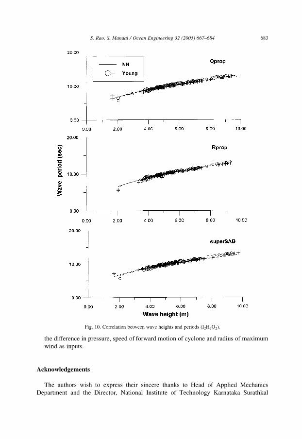
Fig. 10. Correlation between wave heights and periods (I2H2O2).


the difference in pressure, speed of forward motion of cyclone and radius of maximum

wind as inputs.

Acknowledgements

The authors wish to express their sincere thanks to Head of Applied Mechanics

Department and the Director, National Institute of Technology Karnataka Surathkal


and also Head, Ocean Engineering Division, and the Director, National Institute of

Oceanography, GOA for providing all facilities and permitting to publish the results.

References

Crespo, J.L., Mora, E., 1993. Drought estimation with neural networks. Advances in Engineering Software 18,

167–170.

Deo, M.C., Chaudhari, G., 1998. Tide prediction using neural networks. Computer Aided Civil and Infrastructure

Engineering 13, 113–120.

Deo, M.C., Naidu, C.S., 1999. Real time wave forecasting using neural networks. Ocean Engineering 26, 191–

203.

Fahlman, S.E., 1988. An empirical study of learning speed in back propagation networks. Technical Report,

CMU-CS-88-161, Carnegie-Mellon University, Computer Science Dept, Pittsburgh, PA.

French, M.N., Krajewski, W.F., Cuykendall, R.R., 1992. Rainfall forecasting in space and time using a neural

network. Journal of Hydrology 137, 1–29.

Grubert, J.P., 1995. Prediction of estuarine instabilities with artificial neural networks. ASCE Journal of

Computing in Civil Engineering 9 (4), 266–274.

Kasperkiewicz, J., Racz, J., Dubrawski, A., 1995. HPC strength prediction using neural networks. ASCE Journal

of Computing in Civil Engineering 9 (4), 279–284.

Mandal, S., 2001. Back propagation neural network in tidal level forecasting. Journal of Waterway, Port, Coastal

and Ocean Engineering 127 (1), 54–55.

Mase, H., Sakamoto, M., Sakai, T., 1995. Neural network for stability analysis of rubble-mound breakwaters.

Journal of Waterway, Port, Coastal and Ocean Engineering 121 (6), 294–299.

Rao, S., Mandal, S., Prabhaharan, N., 2001. Wave forecasting in near real time basis using neural networks,

Proceedings of International Conference in Ocean Engineering, ICOE-2001, Ocean Engineering Centre, IIT

Madras 2001 pp. 103–108.

Reidmiller, M., 1994. Advanced supervised learning in multi-layer perceptrons—from backpropagation to

adaptive learning algorithms. Computers Standards and Interfaces, Special issue on Neural Networks, (5).

Reidmiller, M., Braun, H., 1993. A direct adaptive method for faster back propagation learning: the Rprop

algorithm. Proceedings of International Conference in Neural Networks, San Francisco, CA 1993.

Sanil Kumar. V., Mandal S., Manish A. Mulik., Rupali S. Patgoankar., 2001. Estimation of wind speeds and wave

heights from tropical cyclones during 1961 to 1982. Technical Report, NIO/TR-3/2001, National Institute of

Oceanography, Goa.

Tveter, D.R., 2000. Professional Basis of AI backprop, http://www.donveter.com/profbp

Varkey, M.J., Vaithiyanathan, R., Santanam, K., 1996. Wind fields of storms from surface isobars for wave

hindcasting. Proceedings of International Conference in Ocean Engineering (ICOE’96), 502–506.

Vaziri, M., 1997. Predicting Caspian sea surface water level by ANN and ARIMA models. Journal of Waterway,

Port, Coastal and Ocean Engineering 123 (4), 158–162.

Young, I.R., 1988. Parametric Hurricane wave prediction model. Journal of Waterways Port Coastal and Ocean

Engineering 114 (5), 637–652.

http://www.donveter.com/profbp

Hindcasting of storm waves using neural networks

Documents

Transcript of Hindcasting of storm waves using neural networks