
Bid Document For Storm Water Drainage Scheme for Saharsa ...
Upload
khangminh22Category
view
0download
0
Review of Storm Water Models
By Christopher Zoppou
C S I R O L A N D a nd WAT E R
CSIRO Land and Water, Canberra
Technical Report 52/99 December 1999

Review of Storm Water Models
by Christopher Zoppou
ISBN 0 643 06075 8
Technical Report No 52/99December 1999
Integrated Water Management GroupChristian LaboratoryCSIRO Land and WaterCanberra ACT Australia

i
ABSTRACT
This report is part of the CSIRO’s Urban Water Project and it is intended to provide a review of themethods used by models for simulating storm water quantity and quality in an urban environment. Thishas been achieved by examining a number of storm water models in current use. These models representa wide range of capabilities and spatial and temporal resolution. The important features of these modelshave been described in this report. Specific topics covered are: Identifying important urban water qualityparameters. The classification of modelling approaches. Modelling approaches used to estimate waterquantity and quality. These include statistical, empirical, hydraulic and hydrological models. Waterresources management and planning tools, that are included in some urban storm water models, such aseconomic analysis, optimisation and risk analysis are also discussed.
Features of twelve storm water models have been summarised. These models have been chosen becausethey demonstrate how components that are important in managing urban storm water have beenincorporated in a modelling framework. These models have been categorised in terms of theirfunctionality, accessibility, water quantity and quality components included in the model and theirtemporal and spatial scale.
This report is useful to planners, managers and modellers. It will provide planners and managers with anoverview of modelling approaches that have been used to simulate storm water quantity and quality. Inparticular, this review provides managers with an appreciation of the limitations and assumptions made invarious modelling approaches. This review will also benefit modellers by providing a comprehensivesummary of approaches and capabilities of a number of storm water models in current use. This reviewhas also been used to identify potential urban storm water research opportunities.
i
TABLE O F CONTENTS
LIST OF TABLE S................................................................................................................. iii
LIST OF FIGURES ............................................................................................................... iii
LIST OF SYMBOL S ............................................................................................................. iv
1. INTRODUCTION .............................................................................................................1
2. URBAN HYDROLOG Y....................................................................................................2
3. MODELLING APPROACHE S .........................................................................................4
3.1 The Quantity of Storm W ater .........................................................................................................6
3.2 The Quality of Storm Wate r ............................................................................................................7
3.3 Approaches t o Storm Wate r Quantity Estimatio n ....................................................................9
3.3.1 Statistical an d Empirical Model s .............................................................................................103.3.2 Deterministic Models ................................................................................................................................ 11
3.3.2.1 Hydraulic Models .............................................................................................................................. 123.3.2.1.1 Shallow Water Wave Equations .................................................................................................. 123.3.2.1.2 Kinematic Wave Model................................................................................................................. 163.3.2.1.3 Diffusion Wave Model................................................................................................................... 17
3.3.2.2 Hydrological Models ......................................................................................................................... 183.3.2.2.1 Unit Hydrograph............................................................................................................................. 193.3.2.2.2 Lumped Continuity or Storage Models....................................................................................... 193.3.2.2.3 Muskingum Method....................................................................................................................... 203.3.2.2.4 Nonlinear Storage ......................................................................................................................... 20
3.4 Approaches t o Storm Wate r Quality Modellin g ......................................................................203.4.1 Statistical and Empirical Approaches .................................................................................................... 213.4.2 Mass Transport Equation ........................................................................................................................ 223.4.3 Completely Mixed Flow............................................................................................................................ 233.4.4 Plug Flow ................................................................................................................................................... 24
4. OTHER ASPECTS OF URBAN STORM WATER MODELLIN G ..................................24
4.1 Optimisatio n .....................................................................................................................................244.1.1 Linear Programming................................................................................................................................. 254.1.2 Dynamic Programming ............................................................................................................................ 254.1.3 Nonlinear Programming ........................................................................................................................... 26
4.2 Uncertai nty Analysi s ......................................................................................................................264.2.1 Sensitivity Analysis ................................................................................................................................... 274.2.2 Mean Value First-order Second Moment Analysis .............................................................................. 274.2.3 Monte Carlo Simulation............................................................................................................................ 28
4.3 Economic Analysi s .........................................................................................................................28
5. URBAN STORM WATER MODEL S..............................................................................29
6. OTHER URBAN STORM WATER QUANTITY AND QUALITY MODELS................... .38
7. OTHER MODELS CAPABLE OF SIMULATING URBAN STORM WATER QUANTITY
AND QUALIT Y ..............................................................................................................39

Review of Storm Water Models
CSIRO Land and Water Technical Report No. 52/99, December 1999
ii
8. SUMMARY.....................................................................................................................42
9. OPPORTUNITIES IN STORM WATER MODELLING...................................................46
10. REFERENCES............................................................................................................48

Review of Storm Water Models
CSIRO Land and Water Technical Report No. 52/99, December 1999
iii
LIST OF TABLES
Table 2.1 Limits of Water Uses Due to Water Quality Degradation (adapted from Chapman 1992 and Dinius 1987)........ 3
Table 2.2 Sources of Non-point Urban Runoff Pollutants (adapted from Whipple et al. 1983) ........................................... 3
Table 2.3 Typical concentrations of pollutants (adapted from Train 1979, Moore and Ramamoorthy 1984, Ellis 1986,
Tchobanoglous et al. 1987, Chapman 1992, Huber 1992a, Sewards and Williams 1995, Duncan 1995) .................... 4
Table 3.1 Sources, Health and Environmental Consequences of various Contaminants .................................................... 10
Table 5.1 Functionality of Representative Models.............................................................................................................. 32
Table 5.2Components in the Quantity Analysis in Representative Models ........................................................................ 32
Table 5.3 Characteristics of Representative Models (adapted from Nix 1991)................................................................... 33
Table 5.4 Water Quality Parameters Modelled ................................................................................................................... 34
Table 7.1 Basic Processes Influencing Constituents ........................................................................................................... 42
Table 7.2. Interdependence of Constituents (WQRRS) ...................................................................................................... 43
LIST OF FIGURES
Figure 1 Overview of Processes Incorporated in a Storm Water Model ............................................................................... 6
Figure 2 Discharge Hydrograph Used as the Upstream Boundary Condition in the Hypothetical Example ...................... 15
Figure 3 Magnitude of the Individual Terms in the Momentum Equation.......................................................................... 15
Review of Storm Water Models
CSIRO Land and Water Technical Report No. 52/99, December 1999
iv
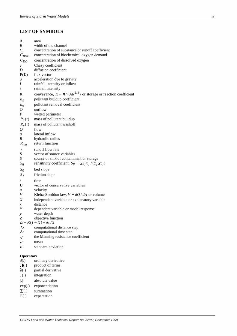
LIST OF SYMBOLS
A areaB width of the channelC concentration of substance or runoff coefficientCBOD concentration of biochemical oxygen demandCDO concentration of dissolved oxygenc Chezy coefficientD diffusion coefficientF(U) flux vectorg acceleration due to gravityI rainfall intensity or inflowi rainfall intensity
K conveyance, K AR K / ( )2/3 or storage or reaction coefficientkB pollutant buildup coefficientkw pollutant removal coefficientO outflowP wetted perimeterP tB ( ) mass of pollutant buildupP tw( ) mass of pollutant washoffQ flowq lateral inflowR hydraulic radiusRi mi, return function
r runoff flow rateS vector of source variablesS source or sink of contaminant or storageSij sensitivity coefficient, S Y x Y xij j j j j ' '/ ( )
S0 bed slopeSf friction slope
t timeU vector of conservative variablesu velocityV Kleitz-Sneddon law, V dQ dA / or volumeX independent variable or explanatory variablex distanceY dependent variable or model responsey water depthZ objective functionD � �K I X t( ) /' 2'x computational distance step't computational time stepK the Manning resistance coefficientP meanV standard deviation
Operatorsd(.) ordinary derivative3(.) product of terms�(.) partial derivative(.)I integration
|.| absolute valueexp(.) exponentiation
(.)Ç summationE[.] expectation
Review of Storm Water Models 1
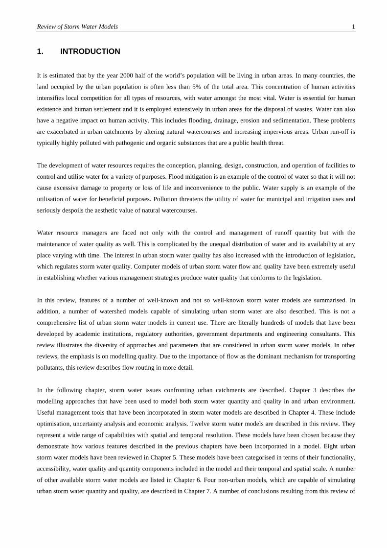
1. INTRODUCTION
It is estimated that by the year 2000 half of the world’s population will be living in urban areas. In many countries, the
land occupied by the urban population is often less than 5% of the total area. This concentration of human activities
intensifies local competition for all types of resources, with water amongst the most vital. Water is essential for human
existence and human settlement and it is employed extensively in urban areas for the disposal of wastes. Water can also
have a negative impact on human activity. This includes flooding, drainage, erosion and sedimentation. These problems
are exacerbated in urban catchments by altering natural watercourses and increasing impervious areas. Urban run-off is
typically highly polluted with pathogenic and organic substances that are a public health threat.
The development of water resources requires the conception, planning, design, construction, and operation of facilities to
control and utilise water for a variety of purposes. Flood mitigation is an example of the control of water so that it will not
cause excessive damage to property or loss of life and inconvenience to the public. Water supply is an example of the
utilisation of water for beneficial purposes. Pollution threatens the utility of water for municipal and irrigation uses and
seriously despoils the aesthetic value of natural watercourses.
Water resource managers are faced not only with the control and management of runoff quantity but with the
maintenance of water quality as well. This is complicated by the unequal distribution of water and its availability at any
place varying with time. The interest in urban storm water quality has also increased with the introduction of legislation,
which regulates storm water quality. Computer models of urban storm water flow and quality have been extremely useful
in establishing whether various management strategies produce water quality that conforms to the legislation.
In this review, features of a number of well-known and not so well-known storm water models are summarised. In
addition, a number of watershed models capable of simulating urban storm water are also described. This is not a
comprehensive list of urban storm water models in current use. There are literally hundreds of models that have been
developed by academic institutions, regulatory authorities, government departments and engineering consultants. This
review illustrates the diversity of approaches and parameters that are considered in urban storm water models. In other
reviews, the emphasis is on modelling quality. Due to the importance of flow as the dominant mechanism for transporting
pollutants, this review describes flow routing in more detail.
In the following chapter, storm water issues confronting urban catchments are described. Chapter 3 describes the
modelling approaches that have been used to model both storm water quantity and quality in and urban environment.
Useful management tools that have been incorporated in storm water models are described in Chapter 4. These include
optimisation, uncertainty analysis and economic analysis. Twelve storm water models are described in this review. They
represent a wide range of capabilities with spatial and temporal resolution. These models have been chosen because they
demonstrate how various features described in the previous chapters have been incorporated in a model. Eight urban
storm water models have been reviewed in Chapter 5. These models have been categorised in terms of their functionality,
accessibility, water quality and quantity components included in the model and their temporal and spatial scale. A number
of other available storm water models are listed in Chapter 6. Four non-urban models, which are capable of simulating
urban storm water quantity and quality, are described in Chapter 7. A number of conclusions resulting from this review of

Review of Storm Water Models
CSIRO Land and Water Technical Report No. 52/99, December 1999
2
storm water models are listed in Chapter 8. Potential urban storm water research opportunities have been identified and
are described in Chapter 9.
2. URBAN HYDROLOGY
Rain falling over a watershed will fall on either an impervious or a pervious area. On a pervious area, some rainfall may
infiltrate the sub-surface and the remainder is surface runoff. Surface runoff and perhaps infiltration will eventually flow
into a watercourse or a receiving water body. This is not the case for an impervious area, where nearly all the rainfall
becomes runoff. An urban area is by definition an area of concentrated human activity, which is characterised by
extensive impervious areas and man made watercourses. The result is an increase in runoff volume and flow that can
result in flooding, watercourse and habitat destruction.
Pollutants are also transported through the urban watershed. Rainfall precipitates atmospheric pollutants. The impact of
rainfall will dislodge particles on the surface of the ground. Many pollutants adhere to these particles and are conveyed
along with soluble pollutants by the runoff. The momentum associated with the runoff dislodges other contaminant-laden
particles. These are transported to a watercourse by the flowing water and progress through the urban watershed.
Pollutants generated on and discharged from land surfaces as the result of the action of precipitation on and the
subsequent movement of water over the land surface, are commonly referred to as non-point pollutants or dispersed
pollutants. Pollutants resulting from the application of water to the land by human activity augment these pollutants.
Depending on the type of activity on the land, the volume of runoff and the amount and types of pollutants carried with it
will vary. The intensity and duration of precipitation and the time since the last precipitation event also affect the quantity
and transport of pollutants generated. Failures in the urban infrastructure (sewer infiltration, leachate from landfills, direct
connection of sanitary sewers to storm water drains) represent another source of pollutant. The diversity in the source and
type of pollutants encountered on an urban catchment makes managing storm water very complicated.
When pollutants discharged into receiving water bodies exceed the assimilation capacity of these bodies, a myriad of
problems can result. Types of biological effects that these water quality problems may cause include; infection of
organisms by bacteria and viruses, death from chronic toxicity exposure and alteration to natural habitat cycles and
breeding. Pollution and water quality degradation can also interfere with the range of legitimate water uses, as shown in
Table 2.1. A similar table can be found in US Environmental Protection Agency (1979). Some types of water uses are
more adversely affected by water quality than others. Many of these problems can be considered as natural phenomena,
which have been exacerbated by man’s activities. The variety of pollutants that can be expected from various non-point
sources in an urban environment are indicated in Table 2.2. Typical concentrations of some of these pollutants are given
in Table 2.3. Pollution from human activity produces waste water and storm water quality that can be detrimental to
human health and to aquatic organisms. Therefore, urban storm water can cause both quality and quantity problems in
receiving waters.

Review of Storm Water Models
CSIRO Land and Water Technical Report No. 52/99, December 1999
3
Table 2.1 Limits of Water Uses Due to Water Quality Degradation
(adapted from Chapman 1992 and Dinius 1987)
Use
Pollutant
Drin
king
Wat
er
Aqu
atic
Wild
life,
Fis
herie
s
Rec
reat
ion
Irrig
atio
n
Indu
stria
l Use
Pow
erG
ener
atio
n
Tra
nspo
rt
Pathogens xx 0 xx x xx1
Suspended Solids xx xx xx x x x2 xx3
Organic Matter xx x xx + xx4 x5
Algae x5,6 x7 xx + xx4 x5 x8
Nitrate xx x + xx1
Salts9 xx xx xx xx10
Trace Elements xx xx x x xOrganic pollutants xx xx x x ?Temperature x xx x x xAcidification x xx x ? x x
xx Marked impairment causing major treatment orexcluding the desired usex Minor impairment0 No impairment+ Degraded water quality may be beneficial for thisspecific use? Effects not yet fully realised
1 food industries2 abrasion
3 sediment settling in channels4 electronic industries5 filter clogging6 odour, taste7 in fish ponds higher algae biomasscan be accepted8 development of water Hyacinth(Eichhomia crassipes)9 also includes boron, fluoride etc.10 Ca, Fe, Mn in textile industries etc.
Table 2.2 Sources of Non-point Urban Runoff Pollutants
(adapted from Whipple et al. 1983)
Source
Vehicles
Pollutant
Soi
l Ero
sion
Wea
r
Exh
aust
Indu
stria
l Was
tes
Fos
sil F
uels
Law
n an
d G
arde
nC
hem
ical
s
Ani
mal
Was
tes
Suspended solids M M MOrganic material M M m MNutrients Nitrogen m M m M M Phosphorus M m M MPetroleumsubstances
M M M
Micro-organisms MHeavy Metals Iron M Manganese M Zinc m M m M Lead M M Copper M M Chromium M M Nickel m M Mercury M Cadmium m MSulfur m M M MAcids Nitric M M Sulfuric M MPesticides M
M major source m minor source
Review of Storm Water Models
CSIRO Land and Water Technical Report No. 52/99, December 1999
4
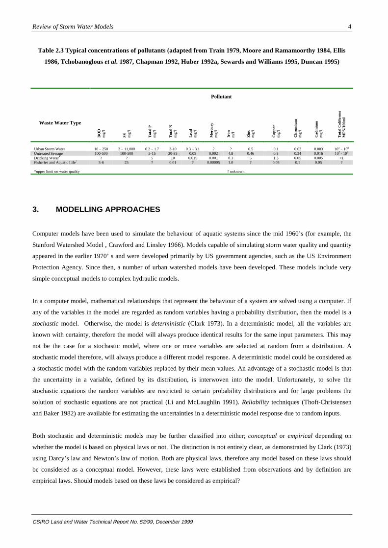
Table 2.3 Typical concentrations of pollutants (adapted from Train 1979, Moore and Ramamoorthy 1984, Ellis
1986, Tchobanoglous et al. 1987, Chapman 1992, Huber 1992a, Sewards and Williams 1995, Duncan 1995)
Pollutant
Waste Water Type
BO
Dm
g/l
SS
mg/
l
Tot
al P
mg/
l
Tot
al N
mg/
l
Lead
mg/
l
Mer
cury
mg/
l
Iron
m/l
Zin
cm
g/l
Cop
per
mg/
l
Chr
omiu
mm
g/l
Cad
miu
mm
g/l
Tot
al C
olifo
rms
MP
N/1
00m
l
Urban Storm Water 10 – 250 3 – 11,000 0.2 – 1.7 3-10 0.3 – 3.1 ? ? 0.5 0.1 0.02 0.003 103 – 108
Untreated Sewage 100-500 100-500 5-15 20-85 0.05 0.002 4.8 0.46 0.3 0.34 0.016 107 - 109
Drinking Water* ? ? 5 10 0.015 0.001 0.3 5 1.3 0.05 0.005 <1Fisheries and Aquatic Life* 3-6 25 ? 0.01 ? 0.00005 1.0 ? 0.03 0.1 0.05 ?
*upper limit on water quality ? unknown
3. MODELLING APPROACHES
Computer models have been used to simulate the behaviour of aquatic systems since the mid 1960’s (for example, the
Stanford Watershed Model , Crawford and Linsley 1966). Models capable of simulating storm water quality and quantity
appeared in the earlier 1970’ s and were developed primarily by US government agencies, such as the US Environment
Protection Agency. Since then, a number of urban watershed models have been developed. These models include very
simple conceptual models to complex hydraulic models.
In a computer model, mathematical relationships that represent the behaviour of a system are solved using a computer. If
any of the variables in the model are regarded as random variables having a probability distribution, then the model is a
stochastic model. Otherwise, the model is deterministic (Clark 1973). In a deterministic model, all the variables are
known with certainty, therefore the model will always produce identical results for the same input parameters. This may
not be the case for a stochastic model, where one or more variables are selected at random from a distribution. A
stochastic model therefore, will always produce a different model response. A deterministic model could be considered as
a stochastic model with the random variables replaced by their mean values. An advantage of a stochastic model is that
the uncertainty in a variable, defined by its distribution, is interwoven into the model. Unfortunately, to solve the
stochastic equations the random variables are restricted to certain probability distributions and for large problems the
solution of stochastic equations are not practical (Li and McLaughlin 1991). Reliability techniques (Thoft-Christensen
and Baker 1982) are available for estimating the uncertainties in a deterministic model response due to random inputs.
Both stochastic and deterministic models may be further classified into either; conceptual or empirical depending on
whether the model is based on physical laws or not. The distinction is not entirely clear, as demonstrated by Clark (1973)
using Darcy’s law and Newton’s law of motion. Both are physical laws, therefore any model based on these laws should
be considered as a conceptual model. However, these laws were established from observations and by definition are
empirical laws. Should models based on these laws be considered as empirical?
Review of Storm Water Models
CSIRO Land and Water Technical Report No. 52/99, December 1999
5
Distributed and lumped models are also used to classify models. These describe how the model treats spatial variability.
A lumped model takes no account of the spatial distribution of the input, whereas distributed models include spatial
variability. Most urban runoff models are deterministic-distributed models (Nix 1994).
Catchment models can be further classified as either event or continuous process driven. Event models are short-term
models used for simulating a few or individual storm events. Continuous models simulate of a catchment’s overall water
balance over a long period of time, involving monthly or seasonal predictions, and form the basis of a planning model for
water resources. Planning models are usually used to estimate the costs associated with different infrastructure
configurations over the life of the infrastructure. Event driven models are suitable for the design of storm water
infrastructure and as operational models. Models that are required to control, operate or allocate water resources in real
time are known as operational models. Flood forecasting models, models used to control weirs and locks in an irrigation
channel and models used to establish what level water is extracted from a reservoir to meet certain water quality
requirements are examples of operational models. Design models refer to models that can be used to model in detail the
flow through the storm water infrastructure.
There will be circumstances where a model can be used for planning, operations and design. The essential difference in
the modelling approaches is the amount of data required, the information that can be obtained from the model, the
sophistication of the analysis performed and the simulation period. For example, a planning model may involve an
optimisation component. Due to the computational effort required in such a model, detailed hydraulic analysis of the
infrastructure is not generally performed. In addition, if infrastructure life cycle costs are modelled, then the simulation
period is of the order of years. Hydraulic modelling at this scale is prohibitive. Urban storm water models have been
adapted for use as operational tools. However, they are more commonly used as either planning or design tools.
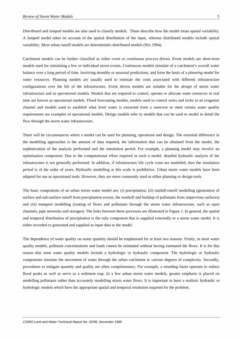
The basic components of an urban storm water model are; (i) precipitation, (ii ) rainfall-runoff modelling (generation of
surface and sub-surface runoff from precipitation excess, the washoff and buildup of pollutants from impervious surfaces)
and (iii ) transport modelling (routing of flows and pollutants through the storm water infrastructure, such as open
channels, pipe networks and storages). The links between these processes are illustrated in Figure 1. In general, the spatial
and temporal distribution of precipitation is the only component that is supplied externally to a storm water model. It is
either recorded or generated and supplied as input data to the model.
The dependence of water quality on water quantity should be emphasised for at least two reasons. Firstly, in most water
quality models, pollutant concentrations and loads cannot be estimated without having estimated the flows. It is for this
reason that most water quality models include a hydrologic or hydraulic component. The hydrologic or hydraulic
components simulate the movement of water through the urban catchment to various degrees of complexity. Secondly,
procedures to mitigate quantity and quality are often complimentary. For example, a retarding basin operates to reduce
flood peaks as well as serve as a sediment trap. In a few urban storm water models, greater emphasis is placed on
modelling pollutants rather than accurately modelling storm water flows. It is important to have a realistic hydraulic or
hydrologic models which have the appropriate spatial and temporal resolution required for the problem.
Review of Storm Water Models
CSIRO Land and Water Technical Report No. 52/99, December 1999
6
3.1 The Quantity of Storm Water
The hydrological cycle begins with precipitation. Precipitation in the form of rain falling on the land surface is subject to
evaporation and initial loss due to interception by vegetation. The excess rainfall is available for infiltration, overland
flow and depression storage. Depression storages are small pore and depressions on the land surface, which temporarily
store water. Infiltrated water may flow through the upper layer of the soil which is generally the unsaturated zone of the
soil, or flow deeper into the soil reaching the groundwater, or saturated zone. Water, which has infiltrated the soil and
moves through the unsaturated zone and later becomes surface water, is known as interflow. In some urban storm water
models, sub-surface flows are not modelled. One reason why sub-surface hydrology is not included in some urban storm
water models is that a large proportion of the urban catchment is impervious, with little or no sub-surface flows.
Unfortunately, accurate representation of the hydrological cycle is important for the accurate simulation of both runoff
and its quality.
The two most important problems associated with the quantity of water are; flooding and water supply. These problems
are relevant in varying degrees to both urban and rural catchments. Alterations to the form of the landscape by human
Figure 1. Overview of Processes Incorporated in a Storm Water Model
Rainfall hyetograph
I
t
Overland FlowRouting
System
Through DrainageFlow Routing
Receiving Waters
Quality ofOverland Flow
Through DrainageQuality Routing
Rainfall-Runoff Module
Transport Module
Q
t
Q
t
C
t
C
t
System
Review of Storm Water Models
CSIRO Land and Water Technical Report No. 52/99, December 1999
7
activity results in increasing runoff volumes, reduced times for flows to reach their maximum and the increase in peak
flow rates. Consequently, urban areas are more susceptible to flooding affecting all land use activities. Provision of storm
water infrastructure, which may consist of a network of drainage pipes, channels and retarding basins is essential to
protect both property and lives from flooding. In many instances, the infrastructure is only designed for a particular
storm event, usually the 1 in 10 year storm event.
The concentration of human activity in a small area also creates problems for supplying water of suitable quality. Water
supply problems relate to the allocation of available water to satisfy various types of water uses, such as industrial,
residential and agricultural. This involves the design of a supply and treatment infrastructure such as reservoirs, pumps,
pipes, reticulation systems and water treatment plants to meet the required demands. Therefore, models developed to
simulate storm water flows from urban areas differ from models developed to estimate flows in rural areas. Models of
urban areas are generally more complicated because they must include additional factors such as gutters, streets, sewers,
overflows, surcharging, closed conduits under pressure, storm water drainage networks, culverts, open channels, roof top
storage, open and natural watercourses and storages. Surcharges occur when a closed conduit, which would normally act
as an open channel, becomes full and acts a conduit under pressure. Under some circumstances, this is desirable because
it has the potential to increase the capacity of the storm water drain. If there is sufficient pressure so that the water rises
above the ground level, then overflow occurs where the excess volume of flow becomes surface runoff. Urban catchments
respond considerably faster to rainfall than rural catchments. Therefore, models developed for an urban catchment must
be able to capture the rapid response of the catchment to storm events.
Another main objective of the analysis of storm water flows is to determine inputs of pollutants to receiving waters.
Flowing water is the main mechanism, along with the impact of rain for transporting pollutants in the urban catchment.
3.2 The Quality of Storm Water
The five natural processes, which affect the movement and transformation of pollutants in an urban catchment are;
chemical, physicochemical, biological, ecological and physical. Chemical processes involve the reaction of two or more
compounds with each other to form one or more different compounds. An example of a chemical process in a natural
system is the transformation of SO2 into SO3 and eventually H2SO4 (sulfuric acid) in the atmosphere. Biochemical
processes are a result of chemical transformations taking place within a biological organism, such as bacterial
decomposition of organic material and photosynthesis. Physicochemical processes involve the chemistry and physics of
molecules interacting with their surroundings. The most important physicochemical processes are; adsorption, desorption
and absorption. Adsorption is the adhesion of a substance to the surface of a solid or liquid. Adsorption is an important
process because many pollutants such as nitrogen, phosphorous, various pesticides and heavy metals attach themselves to
sediment particles and are in turn transported with the particles in flowing water. The quantities of pollutants that become
attached to sediment particles are a function of the concentration of pollutants in the runoff and temperature. Desorption
is the release of pollutants from sediment particles. Absorption is the penetration of a substance into or through another. It
usually takes place at the air-water interface where gases are absorbed into water. This is the primary mechanism whereby
receiving water bodies obtain oxygen. Ecological processes involve interactions between different organisms in the food

Review of Storm Water Models
CSIRO Land and Water Technical Report No. 52/99, December 1999
8
chain. This includes consumption, growth, mortality and respiration from organisms. Transport or physical processes
describe the movement of pollutants by fluid motion. This is primarily by the action of advection, the fluid moving and
diffusion, the motion of molecules and turbulent fluctuations in the fluid dispersing material. The transport process acts
independently of the transformations of nonconservative substances and is equally valid for both conservative and
nonconservative substances. Materials that are not transformed chemically while being transported are termed
conservative substances, otherwise they are nonconservative substances. For example, dissolved salts are conservative
because, generally they do not interact with other substances. Nitrogen, in its ionic state will undergo chemical,
physicochemical and biological transformation in a water body.
Major water quality problems in urban storm water are produced by; salinity, temperature, sedimentation, dissolved
oxygen, toxic substances and biological effects. Temperature has impacts on; physicochemical reactions, biochemical
reactions, biological processes and on the behavioural pattern of organisms. Temperature can also result in synergistic
effects. For example, higher water temperatures exacerbate the adverse effects of low dissolved oxygen concentrations.
Salinity problems are associated with high concentrations of total dissolved salts. Salinity affects aquatic organisms as
well as uses of water withdrawn from receiving water. Sedimentation is a natural process, which has been accelerated in
many areas by man’s activities. Suspended sediments in high concentrations diminish light penetration, thereby inhibiting
photosynthesis by aquatic organisms. Sediments that are deposited can smother plants and organisms and destroy fish
spawning grounds. Sediments entering receiving waters can also carry attached nutrients, pesticides and heavy metals.
Sediments can also clog water treatment plant filters, block channels and pipes. Dissolved oxygen is important as an
indicator of water quality. Organisms in aquatic systems must have oxygen to survive. The primary demand for oxygen in
receiving waters is by decomposing organic material. Three indicators used in relation to oxygen demand are;
biochemical oxygen demand (BOD), chemical oxygen demand (COD) and total organic carbon (TOC). TOC and COD
are an indicator of the total amount of organic material present. BOD is a measure of the total amount of oxygen required
to biochemically oxidise organic matter at a specific temperature and time. It is generally considered a major indicator of
the health of a water body. Toxic substances include; herbicides, insecticides, pesticides, heavy metals, radioactive
materials, oils and reduced ions. The sources, health and environmental consequences of a variety of pollutants that can
occur in urban storm water are given in Table 3.1.
The rates at which chemical, physicochemical and biochemical reactions occur are important in understanding ambient
water quality. However, due to the short response times in urban runoff, impacts of chemical and biochemical processes
on urban runoff quality are usually negligible, the only exception being storages that are used as wetlands. Hence, these
processes are neglected in most urban runoff models.
Modifications which man has made to the land surface have exacerbated physicochemical and transport processes in
many regions, thereby increasing the quantity of pollutants and altering both the types of pollutants and the time pattern
of flows. Consequently, in order to estimate the quantity and quality of water from an urban area, these processes must be
included in a storm water model.
Review of Storm Water Models
CSIRO Land and Water Technical Report No. 52/99, December 1999
9
3.3 Approaches to Storm Water Quantity Estimation
Nix (1994) uses three categories (i) simple, (ii ) simple routing and (iii ) complex routing models to categorise models.
Each category has different demands on data and computing resources and provides results at different time scales and
spatial resolution. In simple models, no routing is performed, little data is required, calculations are not repetitive and a
computer may not be required to perform the calculations. These models provide very little detail of the behaviour of the
flow or pollutant. In general, these models are used to provide long-term averages or peak values. They are specific to a
particular site and catchment behaviour. Empirical models could be considered as simple models. Although some
statistical models are based on complicated techniques, they only reflect the current behaviour of a catchment at a
particular site. Some empirical models involve very simple expressions that do not require the use of a computer. Both
simple and complex routing models are based on physical laws describing the flow within the catchment. Although, they
are deterministic models, they describe the behaviour of the catchment at different complexities. The complexity of a
model has implications on the computational resources required, limitations of the model and the reliability of the results
produced by the model.
The most sophisticated models are capable of producing the same information as simpler models at a price, however the
converse is not generally true. Simple storm water models do not simulate some important processes. For example, the
commonly used storage routing technique is a lumped model. Processes that are time dependent, such as the decay of
some pollutants cannot be modelled because processes are assumed to occur instantaneously. To overcome this problem,
models incorporate time, such as a lag in the routing process. This introduces another subjective parameter for the user to
estimate and this approach is independent of the behaviour of the process being modelled. Lumped models are usually
used in planning models where the time steps are much larger than the time scale of the transients that occur through the
system. Therefore, they use average values for the various processes. This ignores the temporal and spatial variability of
the system, which are required to test the integrity of the storm water system. The spatial and temporal variability must be
artificially introduced into the modelling process. For example, a planning model for allocating potable water may use an
average monthly demand to test a water allocation strategy. However, peak demands are required to test the integrity of
the water supply infrastructure. The assessment of the integrity of the infrastructure is integral to the success of the water
allocation strategy and cannot be performed independent of the water allocation analysis. Therefore, an empirical
relationship between peak and average demands must be established. This adds additional subjectivity and uncertainty in
the modelling process. These problems could be overcome by using models that are more complicated, but at a cost.
The importance of selecting a quantity model with the appropriate temporal and spatial resolution is not emphasised in
other reviews. If flow is not modelled adequately, then water quality predictions will not reflect the true behaviour of the
catchment.
Review of Storm Water Models
CSIRO Land and Water Technical Report No. 52/99, December 1999
10
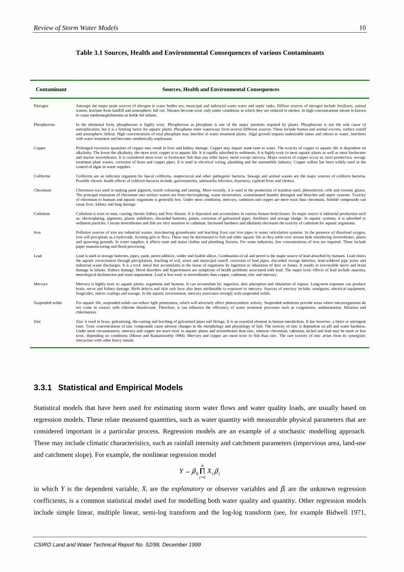
Table 3.1 Sources, Health and Environmental Consequences of various Contaminants
Contaminant Sources, Health and Environmental Consequences
Nitrogen Amongst the major point sources of nitrogen in water bodies are; municipal and industrial waste water and septic tanks. Diffuse sources of nitrogen include fertilisers, animalwastes, leachate from landfill and atmospheric fall out. Nitrates become toxic only under conditions in which they are reduced to nitrites. In high concentrations nitrate is knownto cause methemoglobinemia in bottle fed infants.
Phosphorous In the elemental form, phosphorous is highly toxic. Phosphorous as phosphate is one of the major nutrients required by plants. Phosphorous is not the sole cause ofeutrophication, but it is a limiting factor for aquatic plants. Phosphates enter waterways from several different sources. These include human and animal excreta, surface runoffand atmospheric fallout. High concentrations of total phosphate may interfere in water treatment plants. Algal growth imparts undesirable tastes and odours to water, interfereswith water treatment and becomes aesthetically unpleasant.
Copper Prolonged excessive quantities of copper may result in liver and kidney damage. Copper may impart some taste to water. The toxicity of copper to aquatic life is dependent onalkalinity. The lower the alkalinity, the more toxic copper is to aquatic life. It is rapidly adsorbed to sediments. It is highly toxic to most aquatic plants as well as most freshwaterand marine invertebrates. It is considered more toxic to freshwater fish than any other heavy metal except mercury. Major sources of copper occur in; steel production, sewagetreatment plant wastes, corrosion of brass and copper pipes. It is used in electrical wiring, plumbing and the automobile industry. Copper sulfate has been widely used in thecontrol of algae in water supplies.
Coliforms Coliforms are an indicator organism for faecal coliforms, steptococcal and other pathogenic bacteria. Sewage and animal wastes are the major sources of coliform bacteria.Possible chronic health effects of coliform bacteria include; gartroenteritis, salmonella infection, dysentery, typhoid fever and cholera.
Chromium Chromium was used in making paint pigment, textile colouring and tanning. More recently, it is used in the production of stainless steel, photoelectric cells and ceramic glazes.The principal emissions of chromium into surface waters are from electroplating, waste incineration, contaminated laundry detergent and bleaches and septic systems. Toxicityof chromium to humans and aquatic organisms is generally low. Under most conditions, mercury, cadmium and copper are more toxic than chromium. Soluble compounds cancause liver, kidney and lung damage.
Cadmium Cadmium is toxic to man, causing chronic kidney and liver disease. It is deposited and accumulates in various human body tissues. Its major source is industrial production suchas; electroplating, pigments, plastic stabilisers, discarded batteries, paints, corrosion of galvanised pipes, fertilisers and sewage sludge. In aquatic systems, it is adsorbed tosediment particles. Certain invertebrates and fish are very sensitive to cadmium. Increased hardness and alkalinity decreases the toxicity of cadmium for aquatic organisms.
Iron Pollution sources of iron are industrial wastes, iron-bearing groundwater and leaching from cast iron pipes in water reticulation systems. In the presence of dissolved oxygen,iron will precipitate as a hydroxide, forming gels or flocs. These may be detrimental to fish and other aquatic life as they settle over stream beds smothering invertebrates, plantsand spawning grounds. In water supplies, it affects taste and stains clothes and plumbing fixtures. For some industries, low concentrations of iron are required. These includepaper manufacturing and flood processing.
Lead Lead is used in storage batteries, pipes, paint, petrol additive, solder and fusible alloys. Combustion of oil and petrol is the major source of lead absorbed by humans. Lead entersthe aquatic environment through precipitation, leaching of soil, street and municipal runoff, corrosion of lead pipes, discarded storage batteries, lead-soldered pipe joints andindustrial waste discharges. It is a toxic metal that accumulates in the tissue of organisms by ingestion or inhalation of dust or fumes. It results in irreversible nerve and braindamage in infants. Kidney damage, blood disorders and hypertension are symptoms of health problems associated with lead. The major toxic effects of lead include anaemia,neurological dysfunction and renal impairment. Lead is less toxic to invertebrates than copper, cadmium, zinc and mercury.
Mercury Mercury is highly toxic to aquatic plants, organisms and humans. It can accumulate by; ingestion, skin adsorption and inhalation of vapour. Long-term exposure can producebrain, nerve and kidney damage. Birth defects and skin rash have also been attributable to exposure to mercury. Sources of mercury include; amalgams, electrical equipment,fungicides, mirror coatings and sewage. In the aquatic environment, mercury associates strongly with suspended solids.
Suspended solids For aquatic life, suspended solids can reduce light penetration, which will adversely affect photosynthetic activity. Suspended sediments provide areas where microorganisms donot come in contact with chlorine disinfectant. Therefore, it can influence the efficiency of water treatment processes such as coagulation, sedimentation, filtration andchlorination.
Zinc Zinc is used in brass, galvanising, die-casting and leaching of galvanised pipes and fittings. It is an essential element in human metabolism. It has however, a bitter or astringenttaste. Toxic concentrations of zinc compounds cause adverse changes in the morphology and physiology of fish. The toxicity of zinc is dependent on pH and water hardness.Under most circumstances, mercury and copper are more toxic to aquatic plants and invertebrates than zinc, whereas chromium, cadmium, nickel and lead may be more or lesstoxic, depending on conditions (Moore and Ramamoorthy 1984). Mercury and copper are more toxic to fish than zinc. The rare toxicity of zinc arises from its synergisticinteraction with other heavy metals.
3.3.1 Statistical and Empirical Models
Statistical models that have been used for estimating storm water flows and water quality loads, are usually based on
regression models. These relate measured quantities, such as water quantity with measurable physical parameters that are
considered important in a particular process. Regression models are an example of a stochastic modelling approach.
These may include climatic characteristics, such as rainfall intensity and catchment parameters (impervious area, land-use
and catchment slope). For example, the nonlinear regression model
Y Xii
n ·
E E01
i
in which Y is the dependent variable, Xi are the explanatory or observer variables and βi are the unknown regression
coefficients, is a common statistical model used for modelling both water quality and quantity. Other regression models
include simple linear, multiple linear, semi-log transform and the log-log transform (see, for example Bidwell 1971,

Review of Storm Water Models
CSIRO Land and Water Technical Report No. 52/99, December 1999
11
Jewell and Adrian 1981). Examples of statistical models used in urban watershed modelling can be found in Jewell and
Adrian (1981), Driver and Tasker (1988) and Yao and Terakaura (1999). It is recognised that linear regression is
inadequate in urban catchment modelling (Jewell and Adrian 1981). The most important limitation of statistical models is
that the statistical relationship developed from a given set of data reflects a particular spatial arrangement. For any
markedly different spatial patterns and processes, new data and a new statistical relationship must be developed. Because
of these limitations, the statistical approach has been primarily used only for crude analysis or in situations where
deterministic approaches cannot be used because of insufficient data or resources. Driver and Tasker (1988) describe
regression models as sufficient for planning purposes only.
An example of a regression method for analysing runoff is based on the antecedent precipitation index (API). It is the
most frequently used and important explanatory variable in surface water runoff. The antecedent precipitation index is
essentially the summation of the precipitation amounts occurring prior to the storm, weighted according to the time of
occurrence. An example of a quantity antecedent regression model is (Betson et al. 1969)
C c a dS bA � � �( ) exp( ) ,
Q i C Cn n n � �( ) /1
in which Q is the surface runoff, C runoff coefficient, S a seasonal index parameter, A antecedent precipitation index, i
rainfall and a, b, c, d and n are model coefficients to be determined from the data using regression analysis.
Empirical models involve a functional relationship between a dependent variable and variables that are considered
germane to the process. These variables are chosen from knowledge of the physical processes involved and from
empirical measurements. An example of an empirical approach for estimating runoff is the rational formula
Q CiA .
The rational method is the simplest approach to modelling peak runoff volumes, which are important for storm water
infrastructure design. The rational method is a simple relationship between flow Q, the catchment area A, the rainfall
intensity i, and a runoff coefficient C where 0 ≤ C ≤ 1.
3.3.2 Deterministic Models
Deterministic models are based on conservation laws, which govern the behaviour of a fluid. These laws generally
involve the conservation of flow, known as continuity, the conservation of momentum or the conservation of energy. In
almost all cases, one-dimensional flow analysis is undertaken. Deterministic models used in storm water modelling can
be classified as either hydrologic or hydraulic models. Hydrologic models usually satisfy the continuity equation only.
Hydraulic models solve the continuity equation as well as either the momentum or the energy equations as a coupled
system of equations. The major difference between these modelling approaches is that hydraulic models describe the
spatial behaviour of a process. It is the momentum equation that defines the speed at which a process can occur.
Many engineers in Australia do not make this distinction. The distinction between hydrology and hydraulics is
determined by the process that is being modelled. For example, rainfall-runoff process is considered as a hydrological
process and modelling flows through open channels is a hydraulic problem. This distinction is due to the historical
development of models used to simulate overland and open channel flows. Traditionally, due to the complexity of
Review of Storm Water Models
CSIRO Land and Water Technical Report No. 52/99, December 1999
12
overland flow, only the continuity equation was solved. The dynamic equations (momentum or energy) are considered of
secondary importance. As techniques emerge for simulating overland flow by solving simultaneously the continuity and
dynamic equations, this distinction is not clear. Therefore in this report, the distinction between hydrologic and hydraulic
models is based on the equations that are used to describe a process and not the process that is being modelled.
3.3.2.1 Hydraulic Models
For very simple problems, analytical solutions are available for the solution of the governing equations. Generally,
numerical schemes are used to solve these equations. Hydrological methods have a greater scope for solution using
analytical methods. In complicated problems, numerical schemes such as finite differences, finite elements or the method
of characteristics are used. Finite differences are the most commonly used approach and these can be either implicit or
explicit schemes. In explicit schemes, a single unknown value can be written in terms of known values. This produces a
large number of simple linear equations that can be solved directly for the unknown. In implicit schemes, a number of
unknowns at a particular time are written in terms of the knowns, established previously as well as unknowns at the
current time. This results in a system of coupled simultaneous equations that must be solved. The major advantage with
implicit schemes is that they are unconditionally stable. They are stable for any computational time step used in the
model. Therefore, the additional computational effort required to solve a system of equations is compensated for by a
relaxation in the restriction in the time step that can be used in the simulation. However, the adequate description of
boundary conditions and truncation errors, due to the finite difference approximations, may preclude the use of very large
time steps in an implicit finite difference scheme. This is in contrast to explicit schemes, where there is a severe
restriction on the time step that may be employed. Although the time step restriction is directly proportional to the speed
of the transients being modelled, this may not be a disadvantage in modelling rapidly varying transients. Here a small
time step is required to adequately capture the behaviour of the transient. Rapidly varying transients are common in urban
watershed problems, such as overland flow and flash flooding.
3.3.2.1.1 Shallow Water Wave Equations
The conservative form of the one-dimensional continuity and momentum equations can be written as
�
���
�
U FS
t x(1)
where U is a vector of conservative variables
U �!
"$#
A
Q
F is the flux vector
F U( ) �
�
!
"
$##
Q
Q
AgI
2
1
and S represents the source vector
Review of Storm Water Models
CSIRO Land and Water Technical Report No. 52/99, December 1999
13
S � �
�!
"$#
qA
gA S S gIf( )0 2
in which A is the water depth, Q is the discharge, q is the lateral inflow, x is the distance, t is the time, g is the acceleration
due to gravity, S0 is the bed slope, Sf is the friction slope and I2 is given by
I y x B dy x
10
= −I ( ( ) ) ( ) .( )
ξ ξ ξ
The effects of forces exerted by contraction or expansion of the channel walls on the flow is described by
I y xB
x y x yd
y x
2
00
��
�
I�!
"$#
( ( ) )( )
( )
( )
[[
[
which is zero for a uniform channel, where, B is the width of the channel, y is the water depth and y0 is a constant water
depth. These equations are known as the shallow water wave equations or the St. Venant equations.
The shallow water wave equations written in non-conservative form with the flow velocity u = Q/A and y as the
dependent variables are; for the continuity equation
�
���
�
y
t
uy
xq
( )(2)
and for the momentum equation
10g
u
t
u
g
u
x
y
xS S
q
g
u
yf�
��
�
���
� � � . (3)
The friction slope Sf , is approximated using either the Manning or Chezy equations. The Manning equation is given by
S K Qu u
Rf
2 22
4 3| |
/
K
in which K is the Manning resistance coefficient and R is the hydraulic radius, defined by R = A/P with P the wetted
perimeter and K is known as the conveyance. The Chezy equation is given by
Su u
cRf
| |
in which c is the Chezy resistance coefficient. In both equations, the absolute sign for the velocity will ensure that the
friction always opposes the flow.
The continuity equation, (2) is based on the law of conservation of mass in a fluid element. It simply states that the rate of
change in water depth with time in a fluid element is equal to the net inflow into the fluid element. The momentum
equation, (3) is a mathematical expression for the conservation of momentum within a fluid element. It simply states that
the rate of change in momentum of a fluid element is equal to the sum of forces acting on the element. It is the
momentum equation that determines the velocity or speed of the fluid element.
The shallow water wave equations are hyperbolic and it is this feature that distinguishes them from other methods of
routing, which are generally sub-sets of these equations. The distinguishing feature of the shallow water wave equations
is that they have two characteristics. These characteristics represent the directions that information can travel. In the case
of the shallow water wave equations, depending on the flow conditions, information can propagate both upstream and
Review of Storm Water Models
CSIRO Land and Water Technical Report No. 52/99, December 1999
14
downstream. This is important because downstream obstructions will influence the flow upstream of the obstruction. For
example, flow upstream of a weir will be influenced by the weir. This influence can only be simulated if there is an
interaction of information travelling both upstream and downstream of the weir or obstruction to the flow.
The shallow water wave equations can be used to simulate unsteady one-dimensional gradually and rapidly varying
flows, if (1) is used (see, for example Zoppou and Roberts 1999) in open and natural channels and in pressurised closed
conduits using the Priessmann slot (Abbott 1979). Two-dimensional overland flows can also be simulated using the
shallow water wave equations.
Under steady flow conditions, the continuity equation is simply Q = q, and the momentum equation becomes
S Sd y u g
dxf �
�
0
2 2/2 7(4)
which is used to calculate the water surface profile in an open channel upstream of an obstacle? This type of analysis is
referred to as backwater analysis and it involves the solution of (4) using an iterative scheme (see, for example
Henderson 1966).
In (3) the local acceleration slope, 1/g ∂u/∂t is the same order of magnitude but opposite in sign to the convective
acceleration slope, u/g ∂u/∂x. Both of these terms are generally an order of magnitude smaller than the pressure slope,
∂y/∂x.
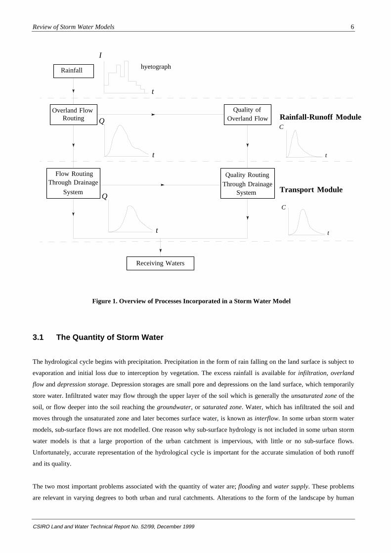
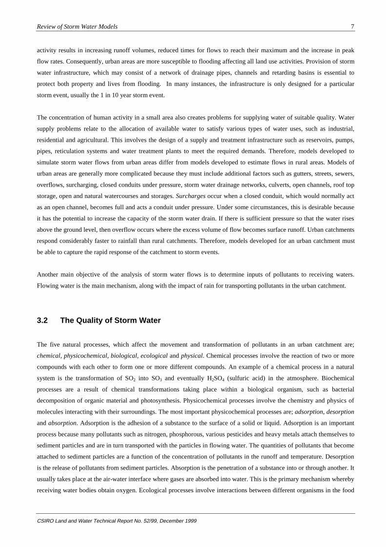
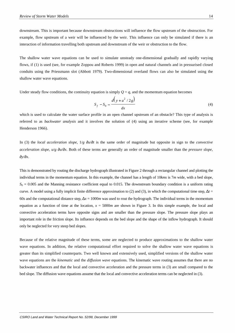
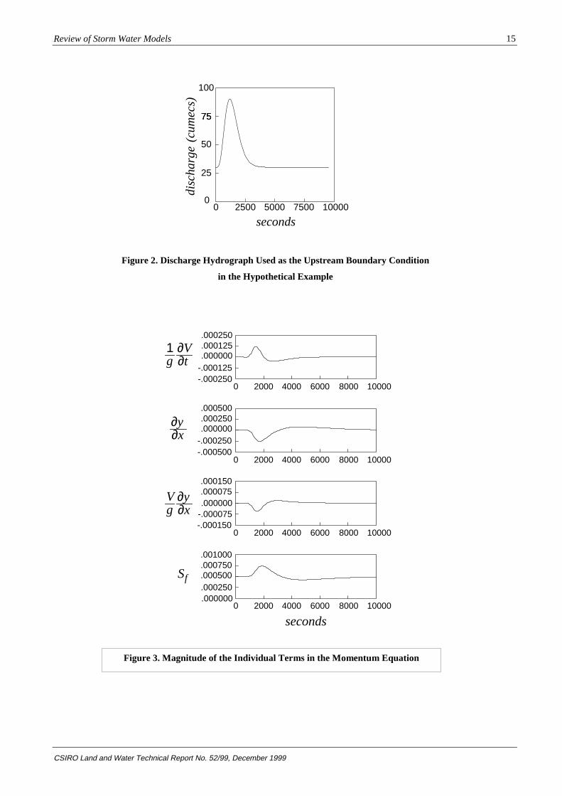
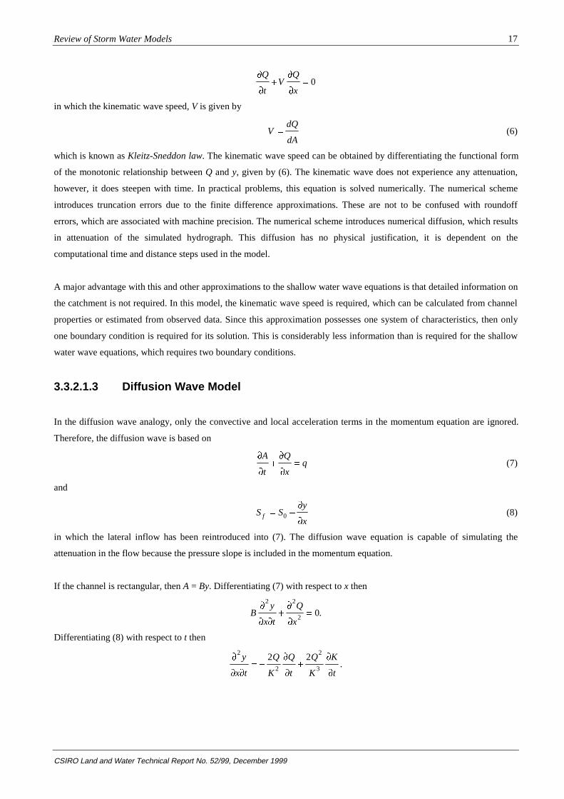
This is demonstrated by routing the discharge hydrograph illustrated in Figure 2 through a rectangular channel and plotting the
individual terms in the momentum equation. In this example, the channel has a length of 10kms is 7m wide, with a bed slope,
S0 = 0.005 and the Manning resistance coefficient equal to 0.015. The downstream boundary condition is a uniform rating
curve. A model using a fully implicit finite difference approximation to (2) and (3), in which the computational time step, ∆t =
60s and the computational distance step, ∆x = 1000m was used to rout the hydrograph. The individual terms in the momentum
equation as a function of time at the location, x = 5000m are shown in Figure 3. In this simple example, the local and
convective acceleration terms have opposite signs and are smaller than the pressure slope. The pressure slope plays an
important role in the friction slope. Its influence depends on the bed slope and the shape of the inflow hydrograph. It should
only be neglected for very steep bed slopes.
Because of the relative magnitude of these terms, some are neglected to produce approximations to the shallow water
wave equations. In addition, the relative computational effort required to solve the shallow water wave equations is
greater than its simplified counterparts. Two well known and extensively used, simplified versions of the shallow water
wave equations are the kinematic and the diffusion wave equations. The kinematic wave routing assumes that there are no
backwater influences and that the local and convective acceleration and the pressure terms in (3) are small compared to the
bed slope. The diffusion wave equations assume that the local and convective acceleration terms can be neglected in (3).
Review of Storm Water Models
CSIRO Land and Water Technical Report No. 52/99, December 1999
15
Figure 3. Magnitude of the Individual Terms in the Momentum Equation
0 2000 4000 6000 8000 10000
.000250
.000125
.000000-.000125-.000250
-.000075
0 2000 4000 6000 8000 10000
0 2000 4000 6000 8000 10000
0 2000 4000 6000 8000 10000
seconds
.001000
.000750
.000500
.000250
.000000
.000500
.000250
.000000-.000250-.000500
.000150
.000075
.000000
-.000150
1 ∂Vg ∂t
∂y∂x
V ∂yg ∂x
Sf
100
7575
50
25
00 2500 5000 7500 10000
dis
cha
rge
(cu
me
cs)
seconds
Figure 2. Discharge Hydrograph Used as the Upstream Boundary Condition
in the Hypothetical Example

Review of Storm Water Models
CSIRO Land and Water Technical Report No. 52/99, December 1999
16
Approximations to the shallow water wave equations only possess one set of characteristics, which always travel
downstream. For example, the influence of a weir on the upstream water level and flow cannot be simulated by the
kinematic or diffusion wave equations. This may have serious implications in the design of storm water infrastructure.
Transients can move rapidly through an urban catchment. To accurately capture these transients using the shallow water
wave equation, very small time steps may be required of the order of seconds, minutes or hours. For larger time steps,
days, weeks or months, transients may have passed through the system. The computational effort required to solve the
shallow water wave equation for a complicated network of channels or pipes can be resource intensive. Therefore,
hydraulic models based on the solution of the shallow water wave equations are usually restricted to event based or
operation modelling. Solving the shallow water wave equations provides detailed information on the behaviour of the
watershed and produces a more accurate representation of the interaction of the flow and the water depth than other
approximate models. The water depth and flow are parameters that are important in the detailed design of storm water
infrastructure. However, simplified and hydrological models only provide information about one of these variables,
which is usually flow. To obtain the water depth from the flow, an empirical relationship between flow and water depth is
required. For gradually varying flows, this relationship is not unique and can represent a significant source of error (see,
for example Henderson 1966). Therefore, models, which solve the shallow water wave equations, are generally used to
design storm water infrastructure.
Data required for the solution of the shallow water wave equations includes cross-sectional information, roughness
coefficients, boundary conditions and any internal structures. For some catchments, this information may not be
available. Generally, approximations to the shallow water wave equations will require less demanding data requirements.
3.3.2.1.2 Kinematic Wave Model
The kinematic wave model assumes that the local, convective and pressure slopes in the momentum equation can be
neglected. It assumes that the friction slope balances the bed slope only, so that Sf = S0. This assumption is generally valid
for overland flow only. With a monotonic relationship between flow and water depth the kinematic wave is based on the
solution of
�
���
�
A
t
Q
x0 (5)
and
Q f y ( ).
The continuity equation, (5) can be written as
�
��
�
�
Q
t
dQ
dA
Q
x0.
Recalling that
∂∂
+ ∂∂
=Q
t
dx
dt
Q
x
dQ
dt
then the kinematic wave equation is given by
Review of Storm Water Models
CSIRO Land and Water Technical Report No. 52/99, December 1999
17
�
��
�
�
Q
tV
Q
x0
in which the kinematic wave speed, V is given by
VdQ
dA (6)
which is known as Kleitz-Sneddon law. The kinematic wave speed can be obtained by differentiating the functional form
of the monotonic relationship between Q and y, given by (6). The kinematic wave does not experience any attenuation,
however, it does steepen with time. In practical problems, this equation is solved numerically. The numerical scheme
introduces truncation errors due to the finite difference approximations. These are not to be confused with roundoff
errors, which are associated with machine precision. The numerical scheme introduces numerical diffusion, which results
in attenuation of the simulated hydrograph. This diffusion has no physical justification, it is dependent on the
computational time and distance steps used in the model.
A major advantage with this and other approximations to the shallow water wave equations is that detailed information on
the catchment is not required. In this model, the kinematic wave speed is required, which can be calculated from channel
properties or estimated from observed data. Since this approximation possesses one system of characteristics, then only
one boundary condition is required for its solution. This is considerably less information than is required for the shallow
water wave equations, which requires two boundary conditions.
3.3.2.1.3 Diffusion Wave Model
In the diffusion wave analogy, only the convective and local acceleration terms in the momentum equation are ignored.
Therefore, the diffusion wave is based on
�
���
�
A
t
Q
xq (7)
and
S Sy
xf �
�
�0 (8)
in which the lateral inflow has been reintroduced into (7). The diffusion wave equation is capable of simulating the
attenuation in the flow because the pressure slope is included in the momentum equation.
If the channel is rectangular, then A = By. Differentiating (7) with respect to x then
By
x t
Q
x
�
� ���
�
2 2
2 0.
Differentiating (8) with respect to t then
�
� � �
�
��
�
�
2
2
2
3
2 2y
x t
Q
K
Q
t
Q
K
K
t.
Review of Storm Water Models
CSIRO Land and Water Technical Report No. 52/99, December 1999
18
Eliminating the second derivative of the flow depth between these equations yields
�
�
�
��
�
�
2
2 2
2
32 2Q
xQBK
Qt
Q BK
Kt
. (9)
Using the continuity equation then
�
�
�
� �
�
�
���
���
K
t
dK
dy
y
t
dK
dy
q
B B
Q
x
1
and substituting into (9) results in an equation in terms of Q as
�
��
�
�
�
��
Q
tV
Q
xD
Q
xS
2
2
in which V is the wave speed and D is a diffusion coefficient, has the form of an advective-diffusion model. The
coefficients are given by
and VQ
KB
dK
dyD
K
QBS
q
KB
dK
dy , .
2
2
For nearly prismatic channels, with the assumption that the pressure slope is small, then V is given by the Kleitz-Sneddon
law and the diffusion equation is simply given by (6).
Price (1973) provides values for these coefficients for an irregular channel, which are functions of the channel properties.
The diffusion wave equation is capable of approximating the physical attenuation experienced by the flow because the
pressure slope is included in the momentum equation.
Cunge (1969) showed that an implicit finite difference approximation of the kinematic wave equation is a second-order
approximation of the diffusion equation. He equated the numerical diffusion and wave speed in the kinematic wave
approximation with the corresponding coefficients in the diffusion equation using a Taylor series expansion of the finite
difference equations. This provides expressions for the computational distance step and a finite difference weighting
coefficient in terms of channel parameters and the computational time step used in the model. This produced the well-
known Muskingum-Cunge method.
3.3.2.2 Hydrological Models
Hydrological methods ignore the spatial variability in the problem. They are generally based on the conservation of mass
only. The unit hydrograph, lumped continuity or storage models, the Muskingum method and nonlinear storage are
considered here to be hydrological methods. Some hydrological models can be interpreted as hydraulic models. The
Muskingum method is one approach that can be described as an approximation to the shallow water wave equations or in
terms of the conservation of mass.

Review of Storm Water Models
CSIRO Land and Water Technical Report No. 52/99, December 1999
19
3.3.2.2.1 Unit Hydrograph
For a storm of given duration, the unit hydrograph is defined as the hydrograph resulting from direct runoff produced by a
unit of rainfall excess over a catchment. Hydrographs for storms of the same duration but different intensity can be
obtained from the unit hydrograph by assuming a linear relationship between the hydrographs. The ordinates of the unit
hydrograph are multiplied by the actual excess runoff depth for the storm. These unit hydrographs can be measured from
individual catchments. More commonly, the unit hydrograph is obtained using analytical techniques. For example, the
linear instantaneous unit hydrograph assumes that the catchment acts as a reservoir and the outflow is a linear function of
storage, so that
S KO
in which S is the storage, O is the outflow and K > 1 is a constant storage coefficient. Combined with the continuity
equation for the reservoir
dS
dtI O �
where I is the inflow, the exponential form of the instantaneous unit hydrograph for a single linear storage is (Chow
1964)
O tK
t K( ) exp( / ). �1
A large catchment can be subdivided into equal sub-catchments with each sub-catchment considered as a separate linear
storage. The instantaneous unit hydrograph for a cascade of n linear reservoirs is given by (Nash 1957)
O tK n
t
Kt K
n
( )( )!
exp( / ) �
����
���
�
1
1
1
which resembles a Gamma function. This model is linear because K is constant and does not consider translation of the
flow. Nonlinear models (Kulandaiswamy 1964) and models which include translation, (Dooge 1959) have been
developed.
3.3.2.2.2 Lumped Continuity or Storage Models
Lumped continuity or storage models simply satisfy the conservation of mass. The catchment response is instantaneous
because the momentum equation is completely ignored. Replacing the spatial derivatives in (5) with finite differences so
that � � �Q x I O x/ /1 6 ' then
dS
dtI O �
in which the storage S A x ' . This equation is known as the storage equation which is used in simple routing methods.
If the flow is assumed to be steady, then dS/dt = 0 and the flow model is simply a mass balance (I = O).
The Modified Puls method solves the storage equation, which is expressed over a finite time interval, ∆t as
' ' 't I I S S tO( ) / 21 2 1 1 2 2 .� � � �tO / 2 (10)

Review of Storm Water Models
CSIRO Land and Water Technical Report No. 52/99, December 1999
20
All the unknowns are on the right hand side of the equation. This method only requires the construction of two curves, S
and S + ∆tO/2 as a function of O. For an initial outflow O1, the storage S1 is obtained from the S – O curve and the
quantity S1 – ∆tO1/2 can be computed. The average inflow plus the quantity S1 + ∆tO1/2 gives the quantity S2 + ∆tO2/2.
Thus the outflow O2 corresponding to S2 – ∆tO2/2 can be determined from the S + ∆tO/2 – O curve. Colon and McMahon
(1987) found that this routing method produced significant errors in the simulated reservoir water depth, the discharge
from the reservoir and in the duration of a flood. This was most pronounced under severe flood or reservoir release and
during non-uniform spatial and temporal precipitation distributions. Under these conditions, the solution of the shallow
water wave equations would be more appropriate.
3.3.2.2.3 Muskingum Method
In the Muskingum method, it is recognised that the storage in a river or reservoir depends on the inflow as well as the
outflow. It is assumed that the storage is a linear function of inflow and outflow, such that
S K XI 1 X O � �( ( ) )
in which K and X are empirical constants to be determined by trial and error. Substituting into (9) and after simplifying
O C I C I C O2 1 2 2 1 3 1 � �
in which
CKX - t / 2
, C
KX t /
, C
KX - t /
K(1 X) t / .1 2 3
� � �
' ' ''
D D DD
2 2and 2
3.3.2.2.4 Nonlinear Storage
In the nonlinear storage methods, the storage is expressed as a nonlinear function of outflow so that
S KOwm
where
O XI X Ow � �( )1
and m is some power. Substituting into the discretised storage equation (9), then
O t KO I I O t KOwm
wm
2 2 1 12 22 1
' '� � � �( ) .
All the terms on the right hand side are known. Since this equation is nonlinear, an iterative scheme is required for its
solution. If m = 1 then the model is identical to the linear Muskingum method.
3.4 Approaches to Storm Water Quality Modelling
Water quality modelling approaches are very similar to those used to model water quantity. Statistical and empirical
models are also relevant for the modelling of pollutants. In deterministic models however, the transport of pollutants is
modelled using a single equation, the conservation of mass, which includes the two fundamental transport processes,
advection and diffusion. Advection describes the process by which pollutants are conveyed by moving water. Diffusion is

Review of Storm Water Models
CSIRO Land and Water Technical Report No. 52/99, December 1999
21
the transportation of pollutants in the direction of decreasing gradient by molecular processes or turbulent fluctuations in
the water. This process can occur in quiescent fluid. In general, turbulent diffusion is much larger than molecular
diffusion. The transport of pollutants is dominated by the advection by flowing water. Diffusion is a secondary process. A
one-dimensional analysis of the transport of pollutants is usually undertaken in urban catchments where the
concentrations represent cross-sectional averages (Fisher et al. 1979).
In storm water modelling, pollutants are treated as neutrally buoyant material, which are transported by fluid motion. The
behaviour of the fluid is assumed to be unaffected by the pollutant and can therefore be calculated independently of the
pollutant transformations. This is not the case for example, with a thermal power station discharging highly saline water
into a freshwater body. The difference in density between the two bodies of water may induce density currents in the
flow. In this case, the flow and pollutant models are coupled and must be solved simultaneously. Sediment transport is
another example where the flow and sediment transport should be modelled as a coupled system. However, this is seldom
done.
3.4.1 Statistical and Empirical Approaches
Statistical models for estimating storm water quality are also based on regression analysis between water quality and
relevant explanatory variables (see, for example Driscoll et al. 1979 and Driver and Tasker 1990, Driver and Troutman
1989). Regression models have been widely used to describe event mean concentrations (EMC) and total storm event
load (Huber 1992a).
An important phenomenon relating to solids accumulation and to pollutant generation and discharge from impervious
surfaces is the first flush. The first flush relates to the high concentrations of pollutants, especially solids, which often
occur in the early portion of a runoff event. Material that has accumulated on a surface during dry weather and material
that has previously been deposited in channels and pipes and is scoured by the flow are primary sources of pollutants in
the first flush. The impact of higher rainfall intensities at the beginning of a storm dislodges particles and as the storm
continues, less pollutant is available to be conveyed by the runoff. This also contributes to the first-flush effect. The
wash-off of pollutants is therefore greater near the beginning of a storm. Between storm events, pollutants accumulate on
impervious surfaces. This is known as the buildup process. Urban runoff quality models attempt to incorporate the build
up and wash-off process using an empirical exponential washoff and the buildup functions. In the washoff model, the rate
at which a pollutant is washed off the surface is assumed to be proportional to the availability of the pollutant on that
surface. A typical washoff function is
dP
dtk rPw
w w= −
in which Pw(t) is the mass of pollutant at time t, kw is an empirical pollutant removal coefficient and r is the runoff flow
rate. It has the following solution
P t P k rtw w w( ) ( )exp( )= −0
where PW(0) is the initial pollutant concentration. The buildup function suggested by Novotny (1995) is
dP
dtI k PB
B B= −
Review of Storm Water Models
CSIRO Land and Water Technical Report No. 52/99, December 1999
22
which has the following analytical solution
P t I k t k P k tB B B B B( ) ( exp( )) / ( )exp( )= − − + −1 0
in which PB(t) is the buildup of pollutant load at time t, I is the accumulation of pollutant between storms and kB is the
coefficient of pollutant buildup. The coefficients for both functions are determined from measured concentrations.
3.4.2 Mass Transport Equation
The basic equations that incorporates the advection and diffusion processes and is used to describe the behaviour of a
pollutant in a stream, is the one-dimensional conservative advective-diffusion equation
�
�
�
�
�
��
�
�¹ �
���
���
(A C)
t xA D
C
x xuA C S(C,x,t)x
x x x1 6
in which, C is the thermal energy or constituent concentration, t the time, x is distance, u is the advection velocity, Ax the
cross-sectional area, Dx the diffusion coefficient and S(C,x,t) are all sources and sinks. This equation includes the
advection of pollutant by the flowing water, diffusion of pollutant in the stream, constituent reactions, interactions and
sources and sinks. Assuming that Ax and Dx are constant and using the flow continuity equation
∂
∂+
∂
∂=
(A C)
t xuAx
x1 6 0
then
�
�
�
��
�
��
C
tD
C
zu
C
zSx
2
2
which is the form of the advective-diffusion equation used in models like HEC – 5Q and WQRRS which are included in
this review. The source term includes sinks and sources for conservative pollutants. For non-conservative pollutants, it
can also include a production or loss of a pollutant, with or without interaction with another pollutant. This is known as a
kinetic process. These include the chemical and physicochemical processes. The general form of such terms is
dC
dtC T jj
iif C �( , , )
in which the rate of change in pollutant Ci is dependent on Ci and other pollutants Cj and temperature T. Generally kinetic
processes are adequately described by first-order relationships of the form
dC
dt �KC
in which K is the first-order rate coefficient and the negative sign indicates decay or loss. Zero-order processes are
described by expressions of the form, dC/dt = -K. Second-order processes involve dC/dt ∝ C2. Higher-order or more
complicated expressions could also be used. Chemical reactions can be described by zero-order, first-order, second-order
or third-order processes. Generally, first-order processes are used. Due to the complex interactions in ecological
processes, (see for example Jogenson 1982,1988) second and third-order kinetics is used to describe them.
Some pollutants are usually coupled, that is when one pollutant decays another may be formed or degrade. This will lead
to a set of simultaneous equations. The advantage of first-order processes, which are coupled, is that the overall first-
order rate coefficient is the sum of the first-order rates for the individual pollutants. The dissolved oxygen sag is a good

Review of Storm Water Models
CSIRO Land and Water Technical Report No. 52/99, December 1999
23
example. Receiving water experiences a depletion of dissolved oxygen due to the inflow of organic material. The sag
curve is due to two competing processes. BOD causes the level of dissolved oxygen to drop and re-aeration replaces
dissolved oxygen from the atmosphere. Therefore, two interacting relationships are required to model the sag curve. The
advective diffusion equation is written for each pollutant. These are
�
�
�
��
�
�� �
C
tD
C
zu
C
zSBOD
xBOD BOD
BOD
2
2
dC
dt
BOD
�
�
�
�
�
�� �
C
tD
C
z- u
C
zSDO
xDO DO
DO
2
2
dC
dt
DO
in which CBOD is the concentration of BOD, CDO is the concentration of DO and S represents sources or sinks. The term
dC/dt represents kinetic processes. Generally, these are described by first-order kinetic relationships. The time rate of
change in BOD is assumed to be governed by
dCKBOD
dtK CBOD= − +( 1 3)
in which K1 is the first-order BOD reaction coefficient and K3 is the first-order decay coefficient for the removal of BOD
by sedimentation and adsorption. The term -K1CBOD governs the rate of removal of BOD which is exactly equal to the rate
of removal of dissolved oxygen. In addition, there is a saturation threshold for dissolved oxygen. Therefore, a suitable
first-order reaction for DO is
dCK Cs KDO
DOdt
C CDO DO � � �2 1( )
in which K2 is the first-order re-aeration coefficient and Cs is the saturated dissolved oxygen concentration. The equation
for BOD concentration can be solved independently of the DO equation. However, the DO equation cannot be solved
until CBOD is known. Therefore, the equations can be solved either simultaneously, using an implicit finite difference
scheme or in a two step process using an explicit finite difference scheme, solving for BOD then for DO.
This simple example illustrates a way in which chemical and the transport process are combined. This is a common
approach adopted in many water quality models.
The above transformations are not restricted to the advective-diffusion equation. They can be used with any transport
equations. As with the hydraulic analysis, many water quality models use simplifications to the advective diffusion
equation. These include completely mixed reactor and plug flow.
3.4.3 Completely Mixed Flow
A completely mixed reactor flow is based on the continuity equation only. This simplification is analogous to the storage
equation in the hydraulic analysis. Complete mixing occurs instantaneously. The rate of change in mass of a pollutant is
given by
VC
t
QC
xKCV S
�
� �
�� �
( )
in which V is the volume of the conduit and the equation contains a first-order decay and source term.

Review of Storm Water Models
CSIRO Land and Water Technical Report No. 52/99, December 1999
24
3.4.4 Plug Flow
Plug flow satisfies the continuity equation and includes travel time in the transport process. This is achieved by assuming
that the input of flow over any time step behaves as a plug of fluid with homogenous quality travelling through a storage
or along a channel. The storage consists of a series of these plugs and their retention time in the storage is determined by
the amount of outflow from the storage. Changes in concentration between the plugs can occur during the retention time.
The rate of change with time of a pollutant in plug flow is given by (Tchobanoglous and Schroeder 1987)
∂
∂= −
∂
∂− ±
C
t
Q
A
C
xKC S
4. OTHER ASPECTS OF URBAN STORM WATER MODELLING
Water resources management planning involves the identification and evaluation of various management alternatives that
satisfy certain objectives. These objectives might involve (i) economic factors, often expressed in terms of costs and (ii )
water quality goals, which are often water quality standards imposed by regulatory authorities. Water resources
management models usually include a water quality and quantity modelling component. In addition to describing the
behaviour of the flow and water quality in a catchment, they may also include cost functions for alternative management
strategies. Given the large number of alternative management strategies and constraints that must be satisfied, some
models include an optimisation technique. Optimisation is used to determine optimum values for a given set of decision
variables that will maximise or minimise an objective function, usually cost.
Planning decisions are greatly enhanced if confidence limits, which reflects the uncertainty in the decision making
process can be placed on the results of a model. This uncertainty may arise from; (i) natural or inherent uncertainty
(random variability in the hydrological processes or in costs), (ii ) model uncertainty (from the use of a simplified model
to describe a complex physical process) and (iii ) parameter uncertainty (model parameters are not known with certainty).
Uncertainty analysis is a technique that can be used to quantify uncertainty in the modelling results. Uncertainty analysis
can be used to identify the dominant sources of uncertainty affecting the reliability of the results from a model. This will
focus both data gathering and research activities in an attempt to reduce the uncertainty in these parameters and in the
modelled results.
4.1 Optimisation
Optimisation provides a mechanism to automate a systematic series of executions of a model in search of an optimum
solution from a range of possible outcomes. The best solution may be a minimum in the least cost sense or the largest
improvement for a given investment. This is defined mathematically by the objective function. The coupling of a storm
water model with an optimisation technique represents an important and powerful tool for the management of urban
storm water. Optimisation techniques available include; (i) linear programming, (ii ) nonlinear programming, (iii ) dynamic
programming and (iv) simulated annealing. Simulated annealing (Kirkpatrick et al. 1983) is not commonly employed in
Review of Storm Water Models
CSIRO Land and Water Technical Report No. 52/99, December 1999
25
water resources problems, with other approaches being more common. Examples in water resources projects where
optimisation techniques have been reported are; Allen and Bridgeman (1986), Behera et al. (1999), Brendecke et al.
(1989), Carriaga and Mays (1995), Chu and Yeh (1978), Chung et al. (1989), Diaz and Fontane (1989), Ford et al.
(1981), Labadie et al. (1980), Lansey and Basnet (1991), Lindell et al. (1987), Martin (1983, 1987), Nitivattananon et al.
(1996) and Ostfeld and Shamir (1996).
Optimisation is also used in some models to calibrate model parameters. This is a process whereby the model response is
fitted to an observed catchment response by adjusting a number of model parameters. This is done in an automatic and
systematic way using an optimisation procedure.
4.1.1 Linear Programming
The general form of the linear programming problem is as follows
minimize (or maximize)
subject to for
and for
Z c x
a x b i 1,2,... ,m
x 0 j 1,2,... ,n
j jj 1
n
ij j ij 1
n
j
Ç
� Ç
�
�
in which Z is the objective function, xj are the decision variables, cj, aij and bi are constants, n is the number of decision
variables and m is the number of constraints. The problem consists of minimising a linear objective function subject to a
set of linear constraints. Their advantage is that simple and efficient solution algorithms exist, such as the simplex
algorithm (Press et al. 1992). It is relatively simple to include the nonegativity constraint. This is important when dealing
with physical quantities, for example, the number of pipes must have a positive value. The linearity restriction of linear
programming restricts its applicability. Nevertheless, many water resources problems can be described realistically by
linear objective functions and constraints.
4.1.2 Dynamic Programming
The dynamic programming approach involves decomposing a complex problem into a series of simpler sub-problems,
which are solved sequentially by transferring information from one level to the next level of the computations. These
stages can represent different points in space or time or activities with a decision required at each stage. For an N-stage
problem, the order of the forward computation is
f x f x f x f x f xi i i i N N1 1 2 2 1 1( ) ( ) ( ) ( ) ( )� � ¹¹ ¹ � � � ¹¹ ¹ �� �
in which fi(xi) is the cumulative optimum return for stages 1,2,…, and i given the state of the system is xi. This pattern can
be written as a recursive equation relating the states fi(xi) to fi-1(xi-1) as
f x Rm
c x
m
m
1 1 11
1 1 1
1( ) max { }
,
,
�
and

Review of Storm Water Models
CSIRO Land and Water Technical Report No. 52/99, December 1999
26
f x R f x c i Ni im
c x
i m i i i mi
i mi i
i i( ) max { ( )}, ,2, ... ,
,
, , � �
�
�1 1
in which ci mi, is the penalty for alternative mi for state i and Ri mi, is the return function of a decision. The conversion from
xi-1 to xi is usually referred to as state transformation. Each stage must have a number of other states associated with it.
The states describe the possible conditions in which the system might be at that stage of the computations. The effect of a
decision at each stage of the problem is to transform the current state of the system into a state associated with the next
stage. The connection between various states is defined by a decision. The state of the system represents the link between
successful stages so that when each stage is optimised separately, the resulting decision is automatically feasible for the
entire problem. It also allows for the optimum decision to be made for the remaining stages without checking the effect
future decisions have on decisions made previously. A return function is the utility or cost of each potential state
transformation. The optimality of the decision required at the current stage is judged in terms of its impact on the return
function for the current stage and all subsequent stages.
The recursive equations are the only unifying theory for dynamic programming, it does not provide details on how the
optimisation for each sub-problem is solved. In addition, there is no guarantee that each sub-problem can be solved.
Dynamic programming, although considered as a powerful technique, is generally more difficult to learn and understand
than linear programming.
4.1.3 Nonlinear Programming
Many problems in water resources are nonlinear. In some instances, the problem may be linearised and linear
programming is employed in an iterative scheme where the solution is refined with each iteration. Robust methods are
available for optimising nonlinear functions. Nonlinear optimisation algorithms can be classified broadly as search
methods. The algorithm systematically and automatically searches through all feasible solutions and finds a solution,
which satisfies the objective function. Search techniques such as conjugate gradient and pattern search methods, are
simple to implement with complex models. In many nonlinear programming techniques, the search direction is governed
by the local slope of the function being optimised. Successful moves are generally in a downhill direction. Unfortunately,
this strategy may only locate a local and not the global minimum and the iterative nature of the approach means that
nonlinear programming can be computationally expensive.
4.2 Uncertainty Analysis
Uncertainty analysis can be performed analytically or numerically. For complex problems, numerical techniques are
exclusively used. Numerical reliability techniques include, in order of accuracy; (i) sensitivity analysis, (ii ) mean value
first-order second moment analysis (iii ) point estimate method, (vi) Monte Carlo simulation and (v) Mellin transform.
There are very few applications of the point estimate and Mellin transform to water resources problems. The point
estimate is a relatively new technique and the Mellin transform is restricted to certain functional relationships not
generally satisfied in complicated models. Examples of the application of uncertainty analysis to water resources
problems can be found in Burges and Lettenmaier (1975), Chatterton et al. (1982), Jaffe and Parker (1984), Melching and
Review of Storm Water Models
CSIRO Land and Water Technical Report No. 52/99, December 1999
27
Yoon (1996), Melching et al. (1991), Scavia et al. (1981), Reddy et al. (1996), Tung (1987, 1989,1990), Warwick and
Wilson (1990), Willey (1986), Xu and Goulter (1998), Yeh and Tung (1993) and Zoppou and Li (1992, 1993).
4.2.1 Sensitivity Analysis
Sensitivity analysis is simply establishing the change in model response, Y due to a small perturbation in each k
independent model variables x = (x1,…,xk). The model is considered most sensitive to the parameters that produce the
greatest model response. This is equivalent to estimating the derivative
∂
∂∀
Y
x i.
j
i
Greater resources should be allocated to those parameters that produce the greatest model response. To effectively
compare the sensitivity of a model to various parameters the derivative must be normalised. Therefore, the normal
sensitivity coefficient Sij for output Yj to input xi is given by
SY / Y
x / xij
j j
j j
'
'
in which ∆x and ∆y are the magnitudes of the perturbations and xj and Yi are the reference values for the output and input
variables respectively. Sensitivity analysis does not consider the variability in a parameter. A highly sensitive parameter
that is relatively well defined may have less influence on the reliability of the results from a model than a much less
sensitive parameter that has large uncertainties. In this case, parameter uncertainty must be considered.
4.2.2 Mean Value First-order Second Moment Analysis
Consider a model response that is a function of a single variable, x so that Y = f(x). The function can be expanded as a
Taylor series around x = µx, where µx is the mean value of x to give
Y fdf
dxx
d f
dxxx x x � � � � � ¹ ¹ ¹( ) ( ) ( )P P P
1
2
2
2
where the derivatives df/dx, d2f/dx2,… are evaluated at x = µx. If second and higher-order terms are neglected, the
resulting first-order expression for Y is
Y fdf
dxxx x� � �( ) ( ).P P
Taking the expectation of both sides, then
P PY xE Y f [ ] ( )
That is the expected value of E[Y] is the mean value of Y and is obtained by evaluating f(x) using the mean value of x =
µx. Combining the above results, the variance of Y defined by
V PY xE Y2 2 �[( ) ]
can be approximated by
V P VY x xEdf
dxx
df
dx
22 2
2� �
���
���
�
!
"
$##
���
���( )
Review of Storm Water Models
CSIRO Land and Water Technical Report No. 52/99, December 1999
28
in which σx2 is the variance of x. If Y is dependent on k mutually independent variables x = (x1,…,xk) it can be shown that
P P P V VY x x Yii
k
xfdf
dxk i
��
��Ç
( , ... , )1
22
1
2 and
The components of the output variance represent weights of the input variances multiplied by the square of the sensitivity
of the model output to the input. Therefore, it is relatively simple to extend sensitivity analysis to perform mean value
first-order second moment analysis. The only additional information that is required is the standard deviation of the input
variables, which is a measure of what is not known about the variable. Correlated random variables can be considered in
first-order second moment analysis. Implicit in mean value first-order second moment analysis is that the model response
is linear or approximately linear near the perturbed values. Since only the mean and variance of the model response is
provided in mean value first-order second moment analysis, only a two parameter distribution can be fitted to the model
response so that confidence limits can be inferred from the fitted distribution.
4.2.3 Monte Carlo Simulation
In Monte Carlo simulation, variables are sampled at random from pre-defined probability distributions, with or without
correlation and the distribution of the model response is obtained from repeated simulations. The validity of this model is
not affected by non-linearities in the water quality model. Comparing the standard deviation estimates from Monte Carlo
simulations with those from first-order second moment analysis, provides an indication of the model non-linearity. The
major drawback with Monte Carlo simulation is that the probability distribution of the uncertain parameters must be
known or assumed. This may not be possible if there is insufficient data to establish these distributions. The other major
problem with Monte Carlo simulation is that it can be computationally expensive. In some problems 1000’s of repeated
simulations of the model are required.
Monte Carlo simulation has the advantage of estimating model frequency distributions, but it is computationally
expensive if a large number of random variables are involved in the problem. The cumulative frequency distribution of
the model response is useful in evaluating overall dispersion in the model predictions and in assessing the likelihood of
violating a water quality standard.
The US Environmental Protection Agency (Salhotra et al. 1988) has developed a generic Monte Carlo module for use
with any transport model. The generator can sample from, Normal, log Normal, uniform, exponential, empirical,
triangular and Johnson SB and SU distributions. Correlated random variables can also be generated.
4.3 Economic Analysis
Water resources managers must be able to identify the best management strategy from a number of alternative scenarios.
The best management strategy could be chosen from those alternatives that do not compromise the storm water
infrastructure using hydraulic analysis. Water quality objectives could be used to select the best management strategy.
Economic analysis provides another method for assessing alternative storm water management options. Traditionally,

Review of Storm Water Models
CSIRO Land and Water Technical Report No. 52/99, December 1999
29
economic analysis generally involved a cost-benefit analysis. The use of cost-benefit criteria as a decision-making tool is
a matter of expediency, since they primarily deal with tangible and quantifiable factors and hence they can be analysed
objectively. These tangible factors are commonly referred to as life-cycle costs and include such things as: maintenance,
capital, operating, replacement, disposal and land acquisition costs.
Economists often lump criteria that are difficult to assign a monetary value as externalities. Externalities might include
social well being, national security, regional growth and stability, preservation of natural areas and risk management
costs. It is clear that society also has constraints it wants to impose on projects that do not necessarily have a monetary
value. Traditional cost-benefit analysis does not consider these factors. The problem is that externalities are intangible
and non-quantifiable, hence would be treated rather subjectively. The real question is not whether externalities should be
considered as a planning objective, but rather how they should be considered objectively within the planning framework.
These objectives are not mutually exclusive, in fact they are often conflicting. Contributions to one may only be made at
the expense of the other. For example, the cost of increasing the capacity of a waste water infrastructure to eliminate
overflows may be significantly greater than the cost associated with the overflow. Using cost-benefit analysis to eliminate
overflows in a design may not be economically feasible. However, social acceptance of overflows may reverse the
decision based on a cost-benefit analysis alone. The problem is how a trade-off should occur. Does an intangible social
dis-benefit, in terms of environmental degradation for example, provide sufficient justification for rejecting a project,
irrespective of the cost-benefit objective?
Fortunately, planners do not make the final decision, nor do they pass legislation that may influence planning decisions.
The real decision-making lies with politicians. Planners do however, demonstrate the cost-effectiveness, the social,
environmental and technical feasibility of a project. Therefore, the impacts of life-cycle costs and externalities should be
considered in project design and ranking. An economic analysis of various management strategies can be misleading if
the infrastructure modelling is inadequate.
5. URBAN STORM WATER MODELS
There are literally hundreds of models developed by academic institutions, regulatory authorities, government
departments and engineering consultants that are capable of simulating water quality and quantity in an urban catchment.
The twelve models chosen represent a wide range of capabilities, spatial and temporal resolutions. In addition, they have
been chosen to demonstrate how the features described in the previous sections, have been incorporated into stormwater
models. Eight models were specifically designed to simulate urban storm water quantity and quality. DR3M – QUAL
(Alley and Smith 1982a, 1982b), HSPF (Bicknell et al. 1993, Johanson et al. 1980, Johanson et al. 1984), MIKE –
SWMM, QQS (Geiger and Dorsch 1980), STORM (Hydrologic Engineering Center 1977), SWMM (Huber and
Dickinson 1988, Huber et al. 1984, Roesner et al. 1988), SWMM Level 1 (Heaney et al. 1976) and the Wallingford
Model (Bettess et al. 1978, Price 1978, Price and Kidd 1978). The remaining four models are capable of being adapted
for use in urban storm water problems, and are; BRASS (Colon and McMahon 1987, McMahon et al. 1984), HEC – 5Q
(Hydrologic Engineering Center 1986), QUAL2E – UNCAS (Brown and Barnwell 1987) and WQRRS (Hydrologic
Engineering Center 1978).

Review of Storm Water Models
CSIRO Land and Water Technical Report No. 52/99, December 1999
30
These models have been classified according to (a) the type of modelling that the model can perform, (b) how the water
quality and quantity components are simulated in the model, (c) the water quality constituents that are modelled, (d)
additional features that a model may posses and (e) the accessibility of the model.
(a) Modelling Scale
Table 5.1 indicates which models can be used as planning, operational and design models. Models which are
capable of simulating single or continuous events are shown in Table 5.3.
(b) Water Quantity and Quality Components
The models that are capable of simulating flows in common infrastructure components, such as pipes, open
channel, retarding basins and natural channels are given in Table 5.2. Other infrastructure components that can
be simulated by these models are also given in Table 5.2. Most of the models simulate the rainfall runoff
process, see Table 5.2. The type of routing that is employed in a model; simple storage, hydrologic and hydraulic
routing is given in Table 5.3. The transport processes that are used by each model to rout pollutants are shown in
Table 5.3. These include the use of the advective diffusion equations, plug flow or assuming that complete
mixing has occurred. The method used in the model for transforming pollutants include; empirical, using a
buildup and washoff processes or modelling the adsorption and desorption with sediment (soil loss).
(c) Water Quality Constituents
The types of pollutants that are modelled are shown in Table 5.4. Although not explicitly included in this table,
heavy metals are generally modelled as conservative pollutants adsorbing to suspended and settleable solids.
(d) Other Model Characteristics
Several models also have the capability of undertaking uncertainty analysis, optimisation and costs. Of the
models reviewed, those capable of performing these functions are shown in Table 5.3. None of the models
considered includes all these capabilities. None of the urban storm water models includes uncertainty analysis
and only two consider cost as an important component in urban storm water management. Two models include
parameter optimisation.
(e) Accessibility
Most of the models have been developed by United States government funded agencies. These models are made
available at a nominal cost with very little support. However, some of these models have gained wide acceptance
with user groups formed to overcome the poor documentation and support. These groups are a valuable source
of information experience on the use of these models. In contrast, commercially available models are supported

Review of Storm Water Models
CSIRO Land and Water Technical Report No. 52/99, December 1999
31
by their developers, but they are expensive. In general, source code for public domain software is available.
Commercial software is distributed as executable files. This makes it very difficult to modify, enhance and
develop interfaces with commercial software.
A more detailed description of the capabilities of these models is provided below.
DR3M - QUAL (Alley and Smith 1982a, 1982b)
In US Geological Survey’s Distributed Routing Rainfall-Runoff model (DR3M) an urban drainage basin is represented by
an overland flow element, a channel element, pipe elements and reservoirs. Soil moisture conditions between storms are
considered in the rainfall runoff modelling. Interflow and base flows are not simulated. Rainfall excess is calculated using
soil moisture, evaporation, pervious and impervious areas, length and slope of the subcatchment and parameter
optimisation. Kinematic wave, which is used to route overland and channel segments is solved using either,
characteristics, implicit or explicit finite difference schemes with time steps as small as a minute. Two soil types can be
defined, each with up to six soil moisture and infiltration parameters. Reservoir storage is simulated using linear storage
or the modified Puls method. Up to 99 flow planes, 3 rainfall gauges and up to 60 storms, spanning up to 20 years can be
accommodated by the model. Channels, pipes, reservoirs and junctions may be used to define the catchment. Surcharges
in pipe networks are also handled. Quality is simulated for arbitrary parameters using exponential build-up and wash-off
functions. Removal of accumulated surface pollutants can occur in dry weather by street cleaning. Erosion is simulated
using empirical equations relating sediment yield to peak runoff and its volume. Up to four pollutants can be simulated,
however interactions between pollutants are not permitted. Concentrations of other pollutants are assumed proportional to
the sediment concentration. Plug flow with no decay is used to rout pollutants through the drainage network and storage
basins. The model can be executed using any time step over any time.
HSPF (Bicknell et al. 1993, Johanson et al. 1980, Johanson et al. 1984)
The US Environmental Protection Agency, Hydrological Simulation Program – Fortran (HSPF) was developed in the mid
1970’s to model a broad range of hydrologic and water quality processes in agricultural and rural watersheds. Urban
watersheds can also be simulated. It is considered the most comprehensive and flexible model of watershed hydrology
and water quality available. It is a continuous watershed hydrology and water quality simulation package using hourly
time steps. Land and soil contaminant runoff processes and in-stream hydraulic and sediment-chemical interactions are
simulated.
For overland flow temperature, DO, CO2, (at saturation levels) coliform, nitrogen, phosphorus, pesticides and arbitrary
conservative pollutants are modelled using empirical relationships between pollutant and water as well as sediment yield.
Rainfall-runoff modelling includes snowmelt, water balance in the upper and lower soil storage and groundwater storage
for both pervious and impervious surfaces. Interception, evaporation and evapotranspiration are included in the water
balance along with displacement of soil by rainfall. Deep groundwater storage can become base flow to a stream. Total
stream flow is a combination of overland and base flow. Washoff quality is estimated using linear buildup with washoff

Review of Storm Water Models
CSIRO Land and Water Technical Report No. 52/99, December 1999
32
Table 5.1 Functionality and Accessibility of Representative Models
Functionality Accessibility
Program Name
Planning Operational Design Public Domain Commercial
Urban Models
DR3M – QUAL ✔ ✔ ✔HSPF ✔ ✔ ✔MIKE – SWMM ✔ ✔ ✔ ✔QQS ✔ ✔ ?STORM ✔ ✔SWMM ✔ ✔ ✔SWWM Level 1 ✔ ✔Wallingford Model ✔ ✔ ✔ ✔
Non-Urban Models
BRASS ✔ ✔ ?HEC – 5Q ✔ ✔ ✔QUAL2E – UNCAS ✔ ✔WQRRS ✔ ✔ ✔
✔
Table 5.2 Components in the Quantity Analysis in Representative Models
Model Quantity Component
Program Name
Pip
es
Ope
n C
hann
el
Ret
ardi
ng B
asin
s
Oth
ers
Nat
ural
Str
eam
s
Rai
nfal
l Run
off
Urban Models
DR3M – QUAL ✔ ✔ ✔ ✔ ✔HSPF ✔ ✔ 1 ✔ ✔MIKE – SWMM ✔ ✔ ✔ 2-7 ✔ ✔QQS 3 ✔ ✔ 2 ✔STORM
SWMM ✔ ✔ ✔ 4 ✔SWMM Level 1 ✔Wallingford Model 4 ✔ ✔ 2-5 ✔
Non Urban Models
BRASS ✔ 1 7 ✔ ✔HEC – 5Q 1 ✔QUAL2E – UNCAS ✔WQRRS ✔ 1 ✔ ✔
1 reservoir module2 weirs and pumps3 pressurised pipes
4 gutter and pumps5 surcharges6 bridges7 overland flow

Review of Storm Water Models
CSIRO Land and Water Technical Report No. 52/99, December 1999
33
Table 5.3 Characteristics of Representative Models (adapted from Nix 1991)
Model Characteristics
Routing LevelTime
ModellingScale
Pollutant PredictiveMethod Pollution Transport Optimisation
UncertaintyAnalysis Costs
Model
Sim
ple
Sto
rage
Hyd
rolo
gic
Hyd
raul
ic
Con
tinuo
us
Eve
nt
Em
piric
al
Bui
ldup
and
Was
hoff
Soi
l Los
s
Adv
ectiv
e D
iffus
ion
Equ
atio
n
Com
plet
ely
Mix
ed R
eact
or
Plu
g F
low
Ana
lytic
al
Lin
ear
Pro
gram
min
g
Non
-Lin
ear
Pro
gram
min
g
Dyn
amic
Pro
gram
min
g
Sen
sitiv
ity A
naly
sis
Firs
t-O
rder
Sec
ond
Mom
ent
Mon
te C
arlo
Life
Cyc
le
Ext
erna
litie
s
Urban Models
DR3M – QUAL ✔ ✔ ✔ ✔ ✔ ✔ ✔ ✔ ✔
HSPF ✔ ✔ ✔ ✔ ✔ ✔ ✔ ✔ ✔
MIKE – SWMM ✔ ✔ ✔ ✔ ✔ ✔ ✔ ✔ ✔ ✔ ✔
QSS ✔ ✔ ✔ ✔ ✔ ✔ ✔ ✔ ✔
STORM ✔ ✔ ✔ ✔ ✔
SWMM Level 1 ✔ ✔ ✔ ✔
SWMM 2 ✔ 3 ✔ ✔ ✔ ✔ ✔ ✔ ✔
Wallingford Model ✔ ✔ ✔ ✔ ✔ ✔ ✔ 4 ✔ 5
Non-Urban Models
BRASS ✔ ✔ ✔
HEC – 5Q ✔ ✔ ✔ ✔ ✔ ✔ ✔ 1
QUAL2E – UNCAS ✔ ✔ ✔ ✔ ✔ ✔ ✔
WQRRS ✔ ✔ ✔ ✔ ✔ ✔ ✔
1 flood damages2 flow balance only3 with EXTRAN module
4. advection only5 labour, material and plant costs
rates directly proportional to runoff. Separate washoff functions are used for each pollutant. Pollutants that can be
simulated with the runoff include; temperature, pesticides, sediments, nitrogen, phosphorous, ammonia and conservative
pollutants. Absorption and desorption of pollutants between bed sediments and water is allowed. Settling and re-
suspension of sand, clay and silt sediments are possible. Re-suspension and settling of silts and clays are based on bed
shear stress. Absorption and desorption of many of these pollutants is optional via first-order kinetics. For impervious
surfaces, empirical relationships are used for the washoff, which is a function of runoff and street cleaning. The advection
of pollutant is estimated using plug flows and complete mixing in storages. Overland flow, open and closed channel flow
and sewer routing is with the modified kinematic wave equation incorporating the Manning equation. It flags surcharges
in the sewer system and reservoir routing can be included. Total dissolved solids, chlorides, pesticides, temperature,

Review of Storm Water Models
CSIRO Land and Water Technical Report No. 52/99, December 1999
34
sediment scour and deposition, pH, CO2, algae, nitrate, nitrite, orthophosphorous, total inorganic carbon, DO, BOD,
ammonia, photoplankton, zooplankton and attached algae can be modelled in streams and in storages.
Table 5.4 Water Quality Parameters Modelled
Water Quality Parameter
Model
Tem
pera
ture
Ino
rgan
ic S
uspe
nded
Sol
ids
Org
anic
Sed
imen
t
In
orga
nic
Sed
imen
t
BO
D
Tot
al C
olifo
rm
Tot
al In
orga
nic
Car
bon
Am
mon
ia
Tot
al N
Tot
al P
Dis
solv
ed O
xyge
n
Alk
alin
ity
pH
Sus
pend
ed S
olid
s
Soi
l Ero
sion
Tot
al D
isso
lved
Sol
ids
Oth
ers
Urban Models
DR3M – QUAL 7,9
HSPF ✔ ✔ ✔ ✔ ✔ ✔ ✔ ✔ ✔ ✔ ✔ ✔ ✔ ✔ ✔ 1,2,7,9,10
MIKE - SWMM ✔ ✔ ✔ ✔ ✔ ✔ ✔ ✔ ✔ ✔ ✔ ✔ 10
QQS ✔ ✔ ✔ ✔ 7 9
STORM ✔ ✔ ✔ 6 7
SWMM ✔ ✔ ✔ ✔ ✔ ✔ 3,7,8
SWMM Level 1 ✔ ✔ ✔ 5
Wallingford Model ✔ ✔ ✔ ✔ 3 7 9
Non Urban Models
BRASS 11
HEC – 5Q ✔ 3 ✔ 1 2 ✔ 9,10
QUAL2E – UNCAS ✔ ✔ ✔ 4 1 2 ✔ 9,10
WQRRS ✔ ✔ ✔ ✔ ✔ ✔ ✔ ✔ 1 2 ✔ ✔ ✔ ✔ 9,10
1 nitrates and nitrites2 phosphorous3 CBOD4 ammonia as N5 suspended and volatile solids
6 orthophosphates7 suspended and settleable solids8 oil/grease9 arbitrary pollutants10 aquatic organisms11 no water quality modelled
MIKE - SWMM
This package combines MIKE 11 (Havno et al. 1995) and the well known SWMM (Huber et al. 1984, Huber and
Dickinson 1988, Roesner et al. 1988) models. The merger is intended to use the strengths of MIKE 11 in one-dimensional
unsteady flow modelling, which solves the shallow water wave equations using an implicit finite difference scheme,
replacing the temperamental EXTRAN module in SWMM. The combined model can perform hydrologic, hydraulic and
water quality analysis of storm water and waste water drainage systems, including sewage treatment plants and water

Review of Storm Water Models
CSIRO Land and Water Technical Report No. 52/99, December 1999
35
quality control devices. Pipes, pumps, culverts, retarding, detention ponds, pressurised flow in looped connections and
overflows from sewers can be modelled.
Mass balance is used for runoff computations, which include surface detention, lower soil storage and upper and lower
groundwater storage. Runoff consists of overland and base flow. Two-dimensional overland flooding can also be
simulated using the shallow water wave equation. A sediment budget accounts for erosion and deposition. The advective
diffusion equation is used to simulate the transport of pollutants, which are subject to first-order kinetics. It is also solved
using an implicit finite difference scheme. Dissolved and suspended sediments, BOD, DO, nutrients, macrophytes and
plankton can be simulated.
MIKE – SWMM can interface with the full suite of Danish Hydraulic Institute models. They have been linked with
STORMPAC, a rainfall generation program, the urban sewer network model, MOUSE (Lindberg et al. 1989), MIKE 21
(Dudley et al. 1994) for modelling of estuaries, lagoons and coastal areas, including water quality and STOAT to assess
treatment plant performance. Water quality parameters include; total coliform, total P, total N, DO, temperature,
ammonia, nitrate, heavy metals using kinetic descriptions of absorption/desorption to particles, suspended sediments and
bed sediments and BOD as both dissolved and attached to suspended sediments. Sediments are defined as either cohesive
or non-cohesive according to their size and behaviour. The dynamics of primary production by photoplankton and the
grazing by zooplankton are described. Primary production by benthic vegetation can also be modelled. MOUSE can
perform real-time control simulations and sediment transport in pipe networks. All these models are capable of simulating
water quality and quantity at any temporal and spatial scale. They can be used in design, management and operation of a
diverse range of water resource problems.
QQS (Geiger and Dorsch 1980)
The Quality-Quantity Simulator (QQS) can perform continuous or single event simulation using five-minute time
intervals. It can simulate flows in pipes and channels using an implicit finite difference approximation of the kinematic
wave equations, storage routing, backwater analysis and pipes under pressure. Looped networks, weirs and pumps can be
simulated. Dry weather flow and quality based on empirical relationships, have a diurnal and population dependency.
Washoff function is dependent on the accumulation of dust and the time interval between storms and street sweeping.
Quality routing through channels and pipes, storage units and receiving water is performed using plug flow. Up to four
arbitrary conservative pollutants can be routed. Empirical washoff functions are available for BOD, COD, suspended
solids, settleable solids, total nitrogen, total P and faecal coliform.
STORM: (Hydrologic Engineering Center 1977)
The US Corps of Engineers, Storage, Treatment, Overflow, Runoff Model is capable of simulating runoff and pollutant
loads from urban and rural watersheds in response to precipitation. It is a continuous model using hourly time steps and it
can be used for single events. Using hourly precipitation, runoff from a catchment is simply the accumulation of runoff
from upstream sub-catchment. There is no attempt to rout the runoff through the catchment. Three methods are available
for calculating the hourly runoff; coefficient method, soil-complex-cover method and the unit hydrograph method. The
Review of Storm Water Models
CSIRO Land and Water Technical Report No. 52/99, December 1999
36
runoff coefficient method is identical to that used in SWMM Level 1. Runoff is a linear relationship between runoff and
the precipitation minus rainfall interception. However, here the impervious and pervious runoff coefficients and the
fraction of impervious area are variable and not fixed. Erosion is estimated using an empirical relationship. Two methods
are available to simulate pollutant accumulation. The pollutant accumulation is proportional to the dust and dirt
accumulated or a simpler linear function of time. Washoff is proportional to the amount of pollutant remaining. Pollutants
that are treated as conservative include; suspended and settleable solids, BOD, total nitrogen and orthophosphates.
Coliforms are also modelled. No treatment is assumed to occur in a storage.
SWMM (Huber et al. 1984, Huber and Dickinson 1988, Roesner et al. 1988)
SWMM simulates both water quality and quantity of urban storm water runoff and combined sewer overflow. This is
both a continuous and single event models. Surface runoff is based on rainfall intensities and antecedent moisture
conditions, land use and topography. A simple nonlinear reservoir storage is used to simulate the rainfall-runoff process,
which includes infiltration depression storage, evaporation and surface runoff. Infiltration is routed through upper and
lower subzones and may return as runoff. Surface pollutant allows both linear and nonlinear accumulation with time.
Washoff is simulated as a simple function of runoff or as a first-order decay relationship. Sewer flows are generated using
land use, population density and other factors. Infiltration into the sewer system is dependent on the sewer condition and
groundwater levels. Flows and pollutants are routed through the sewer system using a modified kinematic wave
approximation and assuming complete mixing. Hydrographs along the sewer system are modified to represent storage
and treatment effects. This includes retention time, treatment efficiency as well as estimating costs. Surcharging is not
included. Pollutants in storage systems can be modelled as either complete mixing or plug flow. The stand-alone module
EXTRAN permits SWMM to rout inflow hydrographs through open channel and a closed conduit system using an
explicit numerical solution of the shallow water wave equations. Unfortunately, routing of pollutant loads, sewer
infiltration and dry-weather flows are not currently modelled. Eight conservative pollutants are; suspended solids,
settleable solids, BOD, COD, total nitrogen, total P, oil/grease, total coliforms as well as an arbitrary pollutant and
erosion simulated in surface runoff.
SWMM Level 1: (Heaney et al. 1976)
SWMM Level 1 estimates average annual runoff from a watershed with the minimum of input data. The average annual
runoff is a simple linear function of the average annual precipitation. Losses from rainfall interception are considered.
The runoff coefficient is a function of pervious and impervious areas, with the latter a function of population. Simple
relationships are used to estimate the annual load of pollutant. The pollutants are treated as independent and they are
directly proportional to the average annual precipitation, population density, the effectiveness of street sweeping and the
catchment area. Land uses considered are residential, commercial, industrial and other developed areas. Pollutants
considered are; BOD, suspended solids, volatile solids, total P and total N. Preliminary estimates for costs of storing and
treating storm water pollutants have been included in SWMM Level 1. This is a simple linear function with constant
costs for treatment and storage. The simple cost function is solved analytically to provide a function representing the least

Review of Storm Water Models
CSIRO Land and Water Technical Report No. 52/99, December 1999
37
cost combination of storage and treatment required satisfying a certain level of pollutant removal. SWMM Level 1 is not
implemented on a computer, it is applied with tables and nomographs. It is part of the EPA’s SWMM package.
Wallingford Model (Price 1978, Price and Kidd 1978, Bettess et al. 1978)
The Wallingford model is a suite of models developed at the Hydraulics Research Institute, Wallingford, United
Kingdom. It includes a rainfall-runoff model (WASSP), a simple (WALLRUS) and full dynamic pipe routing model
(SPIDA) and a water quality module (MOSQITO). The model can be applied to storm water or sewer systems or to the
combined system using 15 minute time steps. It has been used for real time operational, design and planning simulations.
Hyetographs can be defined as input if required. Alternatively, synthetic rain storms can be generated using a variety of
techniques including; depth-duration-frequency relationships and the modified Chicago method. An empirical
relationship is used to determine the average spatial rainfall over a catchment using rainfall intensity and a spatial
smoothing factor. The rainfall-runoff model employs a modified rational method, which is essentially the same as the
rational method with the inclusion of a routing coefficient. The routing coefficient incorporates the proportion of
impervious area, soil type, evapotranspiration and antecedent conditions. Five antecedent moisture models are provided.
The runoff is estimated by distributing rainfall between impervious, roofs and pervious areas. The amount of runoff from
these areas is based on area type, catchment slope, initial loss to depression storage and continuing loss by infiltration.
The attenuation caused by surface storage is simulated by a non-linear reservoir storage model. Two empirical runoff
routing models available. One is for catchments up to 1ha and up to 100ha. The latter relationship is nonlinear
relationship and uses area, slope and length of the catchment. Due to the size of a large catchment, the runoff is also
lagged. The time delay is also a nonlinear empirical relationship based on area, bed slope and length of the catchment.
For small catchments, overland flow is routed using two equal linear reservoirs in series with routing coefficients
dependent on rainfall intensity, contributing area and surface slope. The use of SWMM’s runoff model is optional. Four
other runoff modelling approaches are available which utilise simple storages. A time delay is also introduced so that the
peak runoff lags the peak rainfall.
The Muskingum-Cunge method and the solution of the full shallow water wave equations are options for routing flows
through the storm water network. Both defined and user-specified pipes and channels are options. Pressurised pipes are
modelled with either the St. Venant equations using a Preissmann slot or the St. Venant equations with the local
acceleration term neglected. An implicit finite difference scheme is used to solve the equations. The advection equation is
used in the pollution transport process, while diffusion is ignored. Erosion and deposition processes are modelled,
including sedimentation in pipes. Manholes, overflows, tanks, pump wells or storages can be modelled in the pipe
network. Suspended sediments in tanks are assumed to be well mixed with a layer of cleaner water available at the top of
the tank for overflow. Water quality pollutants that can be modelled are BOD, COD, ammonia, kjeldahl nitrogen, total P
and four arbitrary conservative pollutants that may be attached to sediments or in solution.
Buildup of pollutants on impervious surfaces is an empirical relationship, which is based on time. Washoff is also a first-
order decay model that is a function of rainfall intensity. Pollutants that are available to be washed off impervious

Review of Storm Water Models
CSIRO Land and Water Technical Report No. 52/99, December 1999
38
surfaces are BOD, COD, total N, ammonia, total P and four arbitrary pollutants. Washoff pollutants can be transported by
absorption to sediments or in solution.
A dynamic programming technique is used to determine the minimum construction costs of a storm water network using
pipe diameter, trench depth and gradient as the optimised variables. Both existing and proposed designs can be simulated
by taking into account; storm water overflows, on-line and off-line detention storages and pumping stations. The
Wallingford model includes a module for calculating life cycle costs. The cost modelling includes, labour, plant and
materials costs. A number of construction costs such as; excavations, pavement destruction, bedding, backfill etc. are
included in the labour costs.
6. OTHER URBAN STORM WATER QUANTITY AND QUALITY MODELS
A number of publications have compared and summarised the capability of a number of urban storm water models. These
include (Brandstetter 1976, Chu and Bowers 1977, Dendrou 1982, DeVries and Hromadka 1992, Hall 1984, Huber 1986,
1992b, Huber and Heaney 1982, Reckhow et al. 1985, Whipple et al. 1983 and Wurbs 1994). A useful bibliography on
urban storm water modelling can be found in Duncan (1995).
This review is by no means a comprehensive list of urban storm water models. It is meant to provide a brief summary of
the capability and approaches adopted to simulate storm water quantity and quality by a few well, and not so well known
models.
Other urban storm water models include;
(a) Simple models
Regional Hydrologic Regression and Network Analysis Using Generalised Least Squares (GLSNET) (Tasker and
Stedinger 1989)
(b) Continuous models
• Precipitation-Runoff Modelling Systems (PRMS) (Leavesley et al. 1983)
• The Hydrologic Modeling System (HEC-HMS) (Charley et al. 1995)
(c) Single event models
• US Geological Survey Rainfall Runoff Model for Peak Flow Synthesis (Dawdy et al. 1972, Dawdy and O’Donnell
1965)
• Kinematic Wave Generation Model (Woolhiser 1977, Rovey and Woolhiser 1977)
• Battelle Urban Wastewater Management Model (Brandstetter et al. 1973, Brandstetter 1976)

Review of Storm Water Models
CSIRO Land and Water Technical Report No. 52/99, December 1999
39
• Computer Augmented Treatment and Disposal System (Leiser 1974)
• Distributed Routing Rainfall-Runoff Model: Version II (Alley and Smith 1982a)
• Illinois Storm Sewer System Simulation Model (Sevuk et al. 1973)
• Illinois Urban Drainage Area Simulator (ILLDAS) (Terstriep and Stall 1974)
• SOGREAH (SOGREAH 1977)
• Sacramento Catchment Model (Peck 1976)
• TOMCAT (Brown, 1986)
• KINEROS – A Kinematic Runoff and Erosion Model (Woolhiser et al. 1990)
• MIKE – SHE (Danish Hydraulics Institute 1990)
7. OTHER MODELS CAPABLE OF SIMULATING URBAN STORM WATER QUANTITY
AND QUALITY
The models described above have been developed specifically for the modelling of water quality and quantity in an urban
environment. There are other water quality and quantity models of watersheds that are capable of modelling various
components of the urban water problem. Some of these models are described as follows.
BRASS (McMahon et al. 1984, Colon and McMahon 1987)
The Basin Runoff and Streamflow Simulation (BRASS) was developed by the US Army Corps of Engineers to provide
flood management decision support for the operation of a reservoir system in both real-time and as a design model.
Continuous and event based simulations can be performed. It is an interactive hydrologic/hydraulic simulation model,
which includes rainfall-runoff modelling, storage routing through regulated reservoirs and dynamic streamflow routing
capabilities. BRASS incorporates the National Weather Service Operational Dynamic Wave Model (DWOPER) (Fread
1978) which computes unsteady flows in open channels and due to dam failures. It can be used as a continuous or event
based model for design and real time simulations. The model can handle 15 rivers or tributaries, 90 sub-areas and it can
provide hourly runoff and routing for up to 30 days. In continuous simulation, 100 days of rainfall records from a total of
20 rainfall gauges can be simulated. The rainfall-runoff modelling incorporates; evaporation, infiltration, baseflow,
spatial and temporal rainfall distribution. It requires user specified unit hydrographs and infiltration losses to determine
runoff hydrographs from sub-catchments. Infiltration is a function of rainfall, evaporation and soil moisture. Baseflow is
a simple exponential recession, which is a function of time. Storage routing is used to rout sub-area outflows and shallow
water wave equations are used to rout these flows through river channels. The full dynamic analysis includes; bridges,
embankments overtopping and flows through control structures and through a dentric system. The shallow water wave
equations are solved using the stable implicit finite difference scheme. Missing rainfall data is accommodated in BRASS
by interpolation from neighbouring rainfall gauges. No water quality modelling is performed by BRASS.

Review of Storm Water Models
CSIRO Land and Water Technical Report No. 52/99, December 1999
40
HEC – 5Q (Hydrologic Engineering Center 1986)
The Simulation of Flood Control and Conservation Systems (Including Water Quality Analysis) model, HEC – 5Q, has
the ability to decide how to regulate a complex network of reservoirs. The model will define the optimum system
operation for water quality and quantity. The decision criteria consider flood control, hydropower, instream flow
(municipal, industrial, irrigation, water supply, fish habitat) and water quality requirements. The model uses linear
programming to evaluate the optimum reservoir operating rules. Up to ten reservoirs and up to thirty control points can be
considered. Temperature and up to three conservative and three non conservative water quality constituents can be
modelled using
VC
txQ
C
xxA D
C
xQ C Q C VS.x x c i i
�
�
�
��
�
�� � �
2
2' ' 0
A phytoplankton option requires eight constituents; temperature, total dissolved solids, nitrate nitrogen, phosphate
phosphorous, CBOD, ammonia nitrogen and dissolved oxygen. Non-conservative constituents are replaced by first-order
kinetic decay formulations. The model simulates either daily or monthly data. Therefore, its use is restricted to large
catchments. Hydrological streamflow routing methods such as modified Puls and Muskingum are used in HEC – 5Q.
This model also includes the capability to modify the flows to improve water quality at control points using linear
programming. HEC – 5Q provide economic evaluation capabilities for computing average flood damage.
QUAL2E - UNCAS (Brown and Barnwell 1987)
This is a US Environmental Protection Agency model for simulating stream water quality. It was intended for use as a
planning tool and can simulate steady and unsteady transport of pollutants. However, it assumes steady flow. It can
simulate the interaction of up to 15 water quality constituents. These include; dissolved oxygen, BOD, temperature, algae
as chlorophyll a, organic nitrogen as N, ammonia as N, nitrite as N, nitrate as N, organic phosphorous as P, dissolved
phosphorous as P, coliforms, arbitrary non-conservative constituent and three conservative constituents. All parameters
can be simulated as either steady state or dynamic conditions. Diurnal variations in meteorological data on water quality
only can be studied. Other dynamic forcing functions such as flow variations cannot be modelled. Uncertainty analysis
can be performed. This includes sensitivity analysis, first-order and Monte Carlo analysis. This is only applied to the
steady state simulations. A maximum of 25 river reaches containing no more than 20 computational elements per reach
are permitted. Only six river junctions and seven headwater elements and up to 25 input and withdrawal nodes are
allowed. Flow balance is the only routing that is performed by this model. Storage within an element is ignored and flow
is considered as steady. The water depth is estimated by solving the Manning equation.
The basic equation that is used to describe the behaviour of a pollutant in a stream is the one-dimensional conservative
advective-diffusion equation
AC
t xA D
C
x xuA C
dC
dtS C,x,tx x c x
�
�
�
�
�
��
�
�� �
���
��� 1 6 ( )
in which, C is the thermal energy or constituent concentration, t the time, x is distance, u is the advection velocity, Ax the
cross-sectional area, Dx the diffusion coefficient, S(C,x,t) are all sources and sinks and the term dC/dt defines the first-
order kinetics for non-conservative constituents. Coliforms are modelled as non-conservative constituents. These and

Review of Storm Water Models
CSIRO Land and Water Technical Report No. 52/99, December 1999
41
arbitrary non-conservative constituents are modelled as first-order decaying constituents dependent on temperature and do
not interact with other constituents. Sensitivity analysis of model to individual parameters can be performed using the
UNCAS extension to QUAL2E. In first-order analysis and Monte Carlo simulations, the variables are assumed to be
independent.
WQRRS (Hydrologic Engineering Center 1978)
The US Army Corps of Engineers, Water Quality for River-Reservoir Systems (WQRRS) was designed to model water
quality and quantity within an entire catchment. It consists of three independent modules; a reservoir module
(WQRRSR), a stream hydraulic module (SHP) (Hydrologic Engineering Center 1988) and the stream quality module
(WQRRSQ), that can be coupled if necessary. The model is capable of simulating 18 different physical, chemical and
biological water quality parameters in a river or reservoir or a river-reservoir system. It has the capability to rout flows on
open channels using the shallow water wave equations, kinematic wave equations, Muskingum method or using the
modified Puls method. Steady flows using either stage-flow relationships or backwater analysis can also be performed.
Conservative water quality parameters are modelled using the advective diffusion equation
VC
txQ
C
zxA Dc
C
xQ C Q C VSx x i i
�
�
�
��
�
�� � �' '
2
02
in which, C is the thermal energy or constituent concentration, V is the volume, t is the time, x is the space coordinate
(vertical for the reservoir and horizontal for the stream), Qx is the advective flow, Ax is the surface area, Dc is the effective
diffusion coefficient, Qi is the lateral inflow, Ci is the inflow thermal or concentration, Q0 is the lateral outflow and S are
all the sources and sinks. It is interesting to note that this equation is not conservative unless the advection is assumed to
be constant. The source and sink term is limited to external heat fluxes for temperature. It includes settling, first-order
decay, reaeration, chemical transformation, biological uptake and release, growth, respiration and mortality including
predation. For constituents that affix to the bottom or are mobile, their transformation is governed by
VC
tVS
�
� �
The biological and chemical constituents considered are; fish, aquatic insects, benthic animals, zooplankton,
phytoplankton, benthic algae, detritus, organic sediments, inorganic suspended solids, inorganic sediments, dissolved
phosphate, total inorganic carbon, dissolved ammonia, dissolved nitrates, dissolved nitrates, BOD, coliform bacteria, total
alkalinity, total dissolved solids, pH and unit alkalinity. All chemical and biological rate processes occur in an aerobic
environment. In addition to the transport processes, advection and dispersion, other processes included in WQRRS are
shown in Table 7.1. The interdependence of constituents as represented in WQRRS are given in Table 7.2.
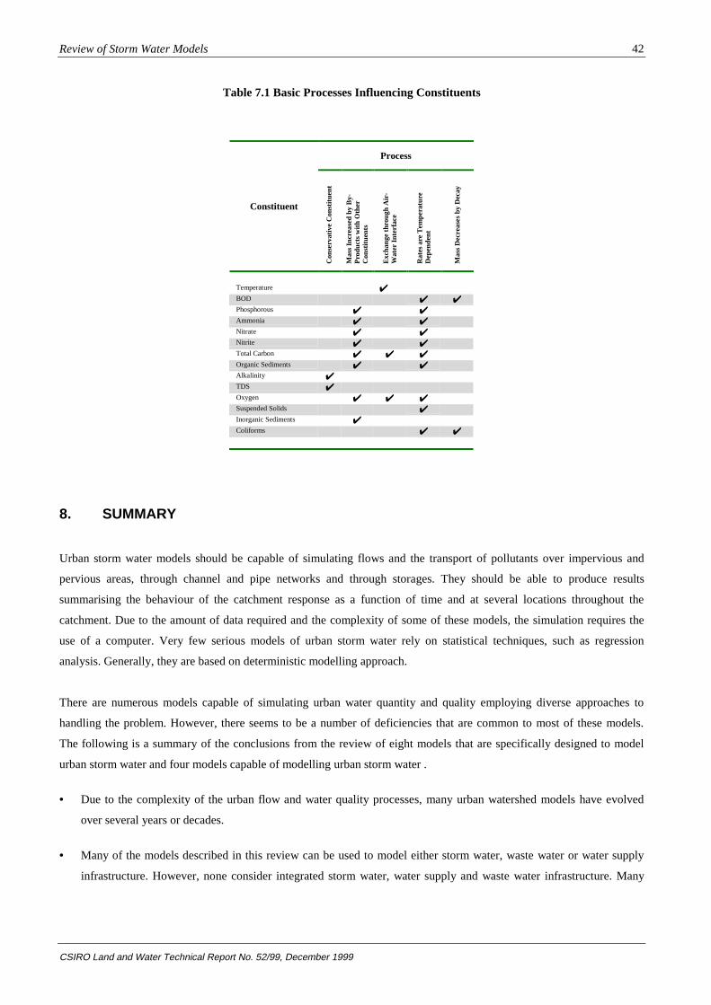
Review of Storm Water Models
CSIRO Land and Water Technical Report No. 52/99, December 1999
42
Table 7.1 Basic Processes Influencing Constituents
Process
Constituent
Con
serv
ativ
e C
onst
ituen
t
Mas
s In
crea
sed
by B
y-P
rodu
cts
with
Oth
erC
onst
ituen
ts
Exc
hang
e th
roug
h A
ir-W
ater
Inte
rfac
e
Rat
es a
re T
empe
ratu
reD
epen
dent
Mas
s D
ecre
ases
by
Dec
ay
Temperature ✔BOD ✔ ✔Phosphorous ✔ ✔Ammonia ✔ ✔Nitrate ✔ ✔Nitrite ✔ ✔Total Carbon ✔ ✔ ✔Organic Sediments ✔ ✔Alkalinity ✔TDS ✔Oxygen ✔ ✔ ✔Suspended Solids ✔Inorganic Sediments ✔Coliforms ✔ ✔
8. SUMMARY
Urban storm water models should be capable of simulating flows and the transport of pollutants over impervious and
pervious areas, through channel and pipe networks and through storages. They should be able to produce results
summarising the behaviour of the catchment response as a function of time and at several locations throughout the
catchment. Due to the amount of data required and the complexity of some of these models, the simulation requires the
use of a computer. Very few serious models of urban storm water rely on statistical techniques, such as regression
analysis. Generally, they are based on deterministic modelling approach.
There are numerous models capable of simulating urban water quantity and quality employing diverse approaches to
handling the problem. However, there seems to be a number of deficiencies that are common to most of these models.
The following is a summary of the conclusions from the review of eight models that are specifically designed to model
urban storm water and four models capable of modelling urban storm water .
• Due to the complexity of the urban flow and water quality processes, many urban watershed models have evolved
over several years or decades.
• Many of the models described in this review can be used to model either storm water, waste water or water supply
infrastructure. However, none consider integrated storm water, water supply and waste water infrastructure. Many

Review of Storm Water Models
CSIRO Land and Water Technical Report No. 52/99, December 1999
43
simply consider only one component, although in the United States, storm water and waste water can share the same
infrastructure and are modelled as a combined system.
Table 7.2. Interdependence of Constituents (WQRRS)
Constituent
Constituent
Tem
pera
ture
Fis
h
Ben
thic
Ani
mal
s
Zoo
pla
nkt
on
Aqu
atic
Inse
cts*
Phy
topl
ankt
on
Ben
thic
Alg
ae*
Det
ritus
Tox
icity
*
Inor
gani
c S
uspe
nded
Sol
ids
Org
anic
Sed
imen
t
Inor
gani
c S
edim
ent
BO
D
Col
iform
Bac
teria
Tot
al In
orga
nic
Car
bon
Am
mon
ia
Nitr
ate
Nitr
ite
Pho
spha
te
Oxy
gen
Alk
alin
ity a
nd
Car
bon
Dio
xide
pH
Temperature K K K K GFish D D D D I D GBenthic Animals L I D GZooplankton L D I GAquatic Insects* L D D I D D D D DPhytoplankton L I D D D DBenthic Algae* L L IDetritus E E,L E J JInorganic Suspended Solids JOrganic Sediments A E JInorganic Sediments J JBOD A GColiform Bacteria ATotal Inorganic Carbon B B B B B B B B G MAmmonia A B B B B B B BNitrate A B GNitrite A B GPhosphate B B B B B B BOxygen F C C C C C C C C C CAlkalinity and TDSCarbon Dioxide F,H M H MpH H H H H
A affects rate of decay, respiration, growth or mortalityB by-Product of decay or respirationC consumed by decay and respirationD prey or nutrients required for growthE by-product of growthF affects reaeration rates and saturationG limits growth or decay if out of acceptable range
H affects chemical EquilibriumI affects mortalityJ source through sedimentation or scourK limits energy input by affecting lightpenetrationL consumed by growth of other constituentsM at chemical equilibrium with otherconstituents* stream module only
• All the urban storm water models can be used as planning models with some as design tools and very few as
operational tools, see Table 5.1. A reason why few urban storm water models are designed as operational models is
that in an urban environment, the transients are very rapid, making it difficult to implement complicated models and
collect data in real-time. Most of the models are capable of simulating single events, see Table 5.3. Those that are
capable of simulating continuous and single events are also used to design urban storm water infrastructure.
• Planning models are continuous models that use simple hydrological approaches to simulate the behaviour of flows
in an urban catchment.

Review of Storm Water Models
CSIRO Land and Water Technical Report No. 52/99, December 1999
44
• All urban storm water models incorporate a rainfall runoff model.
• Spatial distribution of rainfall is not considered in many of these models. Rainfall is assumed to be uniformly
distributed in a subcatchment. The development of a model to interpolate, both spatially and temporally, rainfall data
collected at rainfall gauges, which are sparsely distributed within a catchment, would be a huge advancement in
rainfall runoff modelling.
• For overland flow, the linear storage method is the most popular approach. The shallow water wave equations or
their approximations are seldom employed, although their popularity is increasing.
• Washoff and buildup of pollutants on impervious areas is described by empirical relationship based on first-order
kinetic type relationships.
• Buildup and washoff of pollutants is not very well understood. The simple exponential relationship that is generally
used is not reliable and there are very few data sets available to verify or establish new empirical relationships. More
studies, such as those undertaken by Mackay (1999) are required to establish new or verify these relationships.
• In general, water quality modelling involves first-order kinetics, with adsorption to sediments being a major
component. Very few models have a sediment transport model. This is a conservation of sediment equations which is
solved simultaneously with the shallow water wave equations.
• Simple storage is the most common approach to routing flows. There is a trend towards the use of hydraulic analysis
of storm water infrastructure, with many of the more recently developed models including a number of hydraulic
routing techniques as options.
• The most common water quality parameters that are modelled in urban water storm water models are: BOD, total
coliforms, total P and N and both suspended and bed sediment transport. The non-urban models include arbitrary
conservative pollutants and the modelling of aquatic organisms. Because the effect of pollutants on organisms is
important, temperature, DO and ammonia are also included in non-urban models.
• Design models employ hydraulic modelling for runoff simulation and model the behaviour of storm water flows.
More recently, the St. Venant equations have been solved. This is not due to new techniques being developed to
solve these equations but to the availability of cheaper and more powerful computers making the solution of large
systems of equations more tractable.
• Very few of the models examined have the capability of modelling flash flooding in urban areas. Only MIKE –
SWMM seem to be capable of modelling two-dimensional overland flow.
• Very few model reviews mention the implications of using approximations to the shallow water wave equations. The
shallow water wave equations are capable of simulating the effect of obstacles to the flow, loops in the network and

Review of Storm Water Models
CSIRO Land and Water Technical Report No. 52/99, December 1999
45
pressurised pipe flows. The diffusion wave and kinematic wave equations possess one set of characteristics which
travel downstream. Therefore, these models are not capable of simulating backwater effects from channel and pipe
junctions and obstacles to the flow. In addition, the kinematic wave is not capable of simulating the attenuation in the
flow. The diffusion wave equation approximates the physical attenuation of the flow. This may be a serious
limitation if these models are being used to design storm water infrastructure. Lumped models, which include many
hydrological models, ignore the spatial variability of the problem. This approach assumes that the behaviour of the
catchment is instantaneous. This has serious implications in water quality modelling and other processes that are time
dependent.
• Only one of the urban storm water models solves the advective diffusion equation for the transport of pollutants in
pipes, channels or storages. All the others use simpler techniques, such as plug flow or assuming simply that the
pollutant is completely mixed. This is in contrast to the non-urban models which all use the advective diffusion
equation for the transport of contaminants. Two reasons why the advective-diffusion equation is not solved for urban
problems are: Due to the rapid response of an urban catchment, the transport of contaminants by diffusion is
considered to be insignificant compared to the influence of advection in the transport of these contaminants. Urban
storm water infrastructure networks are generally more complicated than river networks. The numerical solution of
the advective-diffusion equation for complicated networks may be computationally expensive.
• Reliability is another aspect of modelling that is very seldom found in watershed modelling. In view of the
uncertainties in estimating empirical coefficients and the assumed water quality transformation, placing confidence
limits on the model outputs due to these uncertainties should be important and should be an integral part of the
decision making process. Beven (1989) suggests that reliability estimation is a requirement for watershed models.
Risk analysis is a relatively new development in water resources models. The most popular approach is sensitivity
analysis followed by first-order analysis and Monte Carlo simulation.
• Very few storm water models include an economic analysis of alternative storm water strategies. Those that do
include an economic analysis are based only on life cycle costs, externalities are ignored.
• A number of models incorporate an optimisation technique. These are generally used for parameter estimation.
Nonlinear and dynamic programming are almost exclusively used in water resources problems. Only one model
examined uses optimisation to design storm water infrastructure.
• Orlob (1982) commented, that in the late 1970s the technology of modelling, at least that of water quality, reached a
point where advancement seems to depend more on the availability of reliable data from the field than on the
ingenuity of the modeller or on the computer. It seems that this situation has not improved.

Review of Storm Water Models
CSIRO Land and Water Technical Report No. 52/99, December 1999
46
9. OPPORTUNITIES IN STORM WATER MODELLING
This review has highlighted potential research opportunities in storm water modelling, process understanding and data
management. The implementation of many of these research opportunities in a modelling framework is currently
achievable.
(a) Modelling
• Rapidly Varying Flows and Flows over a Dry Bed
One-dimensional unsteady flow models have matured and there have been very few innovative advancements in these
models over the past few years. They are robust, efficient and suitable for simulating gradually varied flows in well
defined channels or conduits. This is not the case for rapidly varying flows and unsteady flows over a dry bed. One and
two-dimensional algorithms for handling these type of flows are emerging. The simulation of flash flooding and storm
water infrastructure failure, which are increasing problems in urban areas, can be modelled with such algorithms.
Accurate modelling of two-dimensional unsteady flows over steep slopes and dry beds is an emerging area of research.
These models will also gain prominence in modelling two-dimensional overland flow.
• Sediment Transport
Adsorption to sediments is a major component in the transport of pollutants. Some models use algorithms that are
abstract. Whilst these may be intuitive, they are often difficult to relate to physical measurements. Sediment transport
models should be more physically based. Sediment transport and flow are co-dependent, therefore the sediment and flow
equations should be solved simultaneously. Very few models solve these equations simultaneously.
• Rainfall Interpolation
Failures in storm water infrastructure are generally associated with high intensity rainfall. The spatial and temporal
variability in rainfall is not adequately considered in rainfall-runoff models. Tools that can accurately interpolate both
spatial and temporal variability in rainfall would provide more reliable estimates of point rainfall and consequently
runoff.
• Integrated Water System
Storm water is only one component of the urban water system. Very few models integrate water resources systems. They
do not include storm water, waste water and potable water systems. Therefore, it is not possible to consider water reuse in
options or the impact of one system on another.
• Economic Analysis
The few storm water models that include economic analysis are based only on life cycle costs. Externalities are ignored.
The occurrence of rare events that result in the failure of urban infrastructure is another emerging aspect of urban storm
water management. Assessing the costs associated with infrastructure failure is seldom included in an economic analysis
of urban systems. For example, flash flooding is disruptive, destructive and places life and property at risk. Recent events
in major city centres in Australia have demonstrated the huge costs associated with the inadequacy of urban infrastructure

Review of Storm Water Models
CSIRO Land and Water Technical Report No. 52/99, December 1999
47
to convey storm water. The costs associated with infrastructure failure are seldom included in the cost of storm water
infrastructure.
• Risk analysis
Uncertainty analysis is not adequately addressed in modelling. Placing confidence limits on the model results, which
reflect the uncertainties in a model, is extremely important. With the model uncertainties quantified, its results can be
viewed in perspective.
• Optimisation
Optimisation has been used in urban storm water models for a number of years. However, they are generally used for
model parameter estimation. There are opportunities for the use of optimisation for the selection of storm water
infrastructure. An obvious example is the use of simulated annealing to size storm water infrastructure.
(b) Process Understanding
• Head Losses in Manholes
Manholes and drop structures in a storm water network can have a significant impact on the behaviour of flow through
these systems. Hydraulic models generally treat these structures as internal boundary conditions. However, their
behaviour under varying flow is not well understood. Laboratory experiments are required to establish the empirical
relationships that accurately reflect the impact of these structures on the flow.
• Buildup and Washoff Function
Most model development activity has been devoted to porting models to personal computers, improving the numerical
procedures or improving their “user friendliness”. This diverts effort from enhancing our understanding of urban runoff
and of better ways to model it. This is particularly true for the accumulation and subsequent transport of pollutants by
runoff. There is a limited knowledge of buildup and washoff of pollutants and methods for simulating the accumulation
and washoff of surface pollutants have not been verified (Nix 1994). The simple exponential relationship that is generally
used is not reliable and there are very few data sets available to verify or establish new empirical relationships. More
studies, such as those undertaken by Mackay (1999), are required to establish new or verify existing relationships.
• Water Quality Interactions
There are numerous algorithms to handle various facets of water quality modelling. Few, if any, are capable of studying a
particular facet with scientific rigour. The interaction of various water quality parameters may have a more significant
influence on an aquatic system that the individual parameters in isolation. Most water quality models ignore or restrict the
interaction of water quality parameters. A greater understanding of the significance of the interaction between water
quality parameters is necessary before reliable algorithms can be developed to describe these interactions.
Review of Storm Water Models
CSIRO Land and Water Technical Report No. 52/99, December 1999
48
(b) Data Management
• Expert System for Model Selection
There are numerous urban storm water models. The level of apparent detail in a model may lead some user to believe that
the results are equally impressive. This is simply not the case. What is required is an expert system that can be used to
assist the user in selecting a model that will balance the modelling effort with the needs of the study.
• Data Archives
Models move ahead of the database available to support them (Nix 1994). Large runoff models require large amounts of
expensive data. What is lacking is an intelligent system that streamlines the management of data. The provision of
interfaces with popular data base management software and spreadsheets will increase the utility of existing models and
data.
10. REFERENCES
Abbott, M.B., (1979) A Modelling System for the Design and Operation of Storm-Sewer Networks, Computational
Hydraulics, Ed. M.B. Abbott, Pitman, Chapter 2, 1, 11-39.
Allen, R.B. and Bridgeman, S.G., (1986) Dynamic Programming in Hydropower Scheduling, Journal of Water Resources
Planning and Management, American Society of Civil Engineers, 112(3), 339-353.
Alley, W.M. and Smith, P.E., (1982a) Distributed Routing Rainfall-Runoff Model: Version II, US Geological Survey,
Geological Survey Open File Report 82-344.
Alley, W.M. and Smith, P.E., (1982b) Multi-Event Urban Runoff Quality Model, US Geological Survey, Open File
Report 82-764, Reston , Virginia.
Behera, P.K., Papa, F. and Adams, B.J., (1999) Optimisation of Regional Storm-Water Management Systems, Journal of
Water Resources Planning and Management, American Society of Civil Engineers, 125(2), 107-114.
Betson, R.P., Tucker, R.L. and Haller, F.M., (1969) Using Analytical Methods to Develop a Surface-Runoff Model,
Water Resources Research, 5(1), 103-111.
Bettess, R., Pitfield, R.A. and Price, R.K., (1978) A Surcharging Model for Storm Sewer Systems, Urban Storm
Drainage, Ed. P.R. Halliwell, Pentech Press, London, 306-316.
Beven, K.J., (1989) Changing Ideas in Hydrology: The Case of Physically Based Models, Journal of Hydrology, 105,
157-172.

Review of Storm Water Models
CSIRO Land and Water Technical Report No. 52/99, December 1999
49
Bicknell, B.R., Imhoff, J.C., Kittle, J.L., Donigan, A.S. and Johanson, R.C., (1993) Hydrologic Simulation Program:
Fortran User’s Manual for Release 10, US Environmental Protection Agency, Athens, Georgia, Report EPA/600/R-
93/174.
Bidwell, V.J., (1971) Regression Analysis of Nonlinear Catchment Systems, Water Resources Research, 7(5), 1118-
1126.
Brandstetter, A.B., (1976) Assessment of Mathematical Models for Storm and Combined Sewer Management, US
Environmental Protection Agency, Cincinnati, Ohio, Report EPA/600/2-76-175a.
Brandstetter, A.B., Engel, R.L. and Cearlock, D.B., (1973) A Mathematical Model for Optimum Design and Control of
Metropolitan Wastewater Management Systems, Water Resources Bulletin, 9(6), 1188-1200.
Brendecke, C.M., DeOreo, W.B., Payton, E.A. and Rozaklis, L.T., (1989) Network Modes of Water Rights and System
Operations, Journal of Water Resources Planning and Management, American Society of Civil Engineers, 115(5), 684-
696.
Brown, L.C. and Barnwell, T.O., (1987) The Enhanced Stream Water Quality Models QUAL2E and QUAL2e-UNCAS:
Documentation and Users Manual, US Environmental Protection Agency, Athens, Georgia, Report EPA/600/3-87/007.
Brown, S.R., (1986) TOMCAT: A Computer Model Designed Specifically for Catchment Quality Planning Within the
Water Industry, International Conference on Water Quality Modelling in the Inland Natural Environment, British
Hydraulic Research Association, Cranfield, England, 37-49.
Burges, S.J. and Lettenmaier, D.P., (1975) Probabilistic Methods in Stream Quality Management, Water Resources
Bulletin, 11(1), 242-247.
Carriaga, C.C. and Mays, L.W., (1995) Optimisation Modeling for Sedimentation in Alluvial Rivers, Journal of Water
Resources Planning and Management, American Society of Civil Engineers, 121(3), 251-259.
Chapman, D., (1992) Water Quality Assessments: A Guide to the Use of Biota, Sediments and Water in Environmental
Monitoring, Chapman Hall, London.
Charley, W., Pabst, A. and Peters, J., (1995) The Hydrologic Modeling System (HEC-HMS): Design and Development
Issues, Hydrological Engineering Center, US Army Corps of Engineers, Technical Paper No. 149.
Chatterton, R.A., Miller, A.C. and McDonnell, A.J., (1982) Uncertainty Analysis of Dissolved Oxygen Model, Journal of
the Environmental Engineering Division, American Society of Civil Engineers, 108(EE5), 1003-1013.

Review of Storm Water Models
CSIRO Land and Water Technical Report No. 52/99, December 1999
50
Chow, V.T., (1964) Handbook of Applied Hydrology, McGraw-Hill Cook Co., New York.
Chu, C.S. and Bowers, C.E., (1977) Computer Programs in Water Resources, Water Resources Research Center,
University of Minnesota, WRRC Bulletin 97.
Chu, W.S. and Yeh, W.W.G., (1978) A Nonlinear Programming Algorithm for Real Time Hourly Reservoir Operations,
Water Resources Bulletin, 14(5), 1048-1063.
Chung, F.I., Archer, M.C. and DeVries, J.J., (1989) Network Flow Algorithm Applied to California Aqueduct
Simulation, Journal of Water Resources Planning and Management, American Society of Civil Engineers, 115(2), 131-
147.
Clark, R.T., (1973) Mathematical Models in Hydrology, Irrigation and Drainage Paper, Food and Agriculture
Organization of the United Nations, Rome.
Colon, R. and McMahon, G.F., (1987) BRASS Model: Application to Savannah River System Reservoirs, Journal of
Water Resources Planning and Management, American Society of Civil Engineers, 113(2), 177-190.
Crawford, N.H. and Linsley, R.K., (1966) Digital Simulation in Hydrology, Stanford Watershed Model, Department of
Civil Engineers, Stanford University, Technical Report No. 39.
Cunge, J.A., (1969) On the Subject of a Flood Propagation Method, Journal of Hydraulic Research, 7(2), 205-230.
Danish Hydraulic Institute (1990) MIKE 11 – A Microcomputer Based Modelling System for Rivers and Channels, Users
Manual, Danish Hydraulic Institute, Horsholm, Denmark.
Dawdy, D.R. and O’Donnell, T., (1965) Mathematical Models of Catchment Behaviour, Journal of the Hydraulics
Division, Proceedings of the American Society of Civil Engineers, 91(HY4), 123-137.
Dawdy, D.R., Lichty, R.W. and Bergman, J.M., (1972) A Rainfall-Runoff Simulation Model for Estimation of Flood
Peaks for Small Drainage Basins, US Geological Survey, Professional Paper 506-B.
Dendrou, S.A., (1982) Overview of Urban Stormwater Models, Urban Stormwater Hydrology, Ed., D.F. Kibler,
American Geophysical Union, Washington, DC, 219-247.
DeVries, J.J. and Hromadka. T.V., (1992) Computer Models for Surface Water, Handbook of Hydrology, Ed. D.R.
Maidment, Chapter 12.
Diaz, G.E. and Fontane, D.G., (1989) Hydropower Optimisation via Sequential Quadratic Programming, Journal of
Water Resources Planning and Management, American Society of Civil Engineers, 115(6), 715-734.

Review of Storm Water Models
CSIRO Land and Water Technical Report No. 52/99, December 1999
51
Dinius, S.H., (1987) Design of an Index of Water Quality, Water Resources Bulletin, 23(5), 833-843.
Dooge, J.C.I., (1959) A General Theory of the Unit Hydrograph, Journal of Geophysical Research, 64(1), 241-256.
Driscoll, D., Toro, D.M.D. and Thomann, R.V., (1979) A Statistical Method for Assessment of Urban Runoff, US
Environmental Protection Agency, Washington, DC, Report EPA/440/3-79-023.
Driver, N.E. and Tasker, G.D., (1988) Techniques for Estimation of Storm-Runoff Loads, Volumes, and Selected
Constituent Concentrations in Urban Watersheds in the United States, US Geological Survey, Open File Report 88-191.
Driver, N.E. and Tasker, G.D., (1990) Techniques for Estimation of Storm-Runoff Loads, Volumes, and Selected
Constituent Concentrations in Urban Watersheds in the United States, US Geological Survey, Water Supply Paper 2363.
Driver, N.E. and Troutman, B.M., (1989) Regression Models for Estimating Urban Storm-Runoff Quality and Quantity in
the United States, Journal of Hydrology, 109, 221-236.
Dudley, J., Bryan, D. and Chambers, B., (1994) STOAT – Development and Application of a Fully Dynamic Sewage
Treatment Works Model, International User Group Meeting: Computer Aided Analysis and Operation in Sewage
Transport and Treatment Technology, Goteborg, Sweden.
Duncan, H.P., (1995) A Bibliography of Urban Stormwater Quality, Cooperative Research Centre for Catchment
Hydrology, Report 95/8.
Ellis, J.B., (1986) Pollutional Aspects of Urban Runoff, Urban Runoff Pollution, Eds. H.J. Marsalek and M. Desbordes,
NATA ASI Series, Series G: Ecological Sciences, Vol. 10, Springer-Verlag, Berlin.
Fisher, H.B., List, E.J., Koh, R.C.Y., Imberger, J. and Brooks, N.H., (1979) Mixing in Inland and Coastal Waters,
Academic Press, Boston.
Ford, D.T., Garland, R. and Sullivan, C., (1981) Operation Policy Analysis: Sam Rayburn Reservoir, Journal of Water
Resources Planning and Management, American Society of Civil Engineers, 107(WR2), 339-350.
Fread, D.L., (1978) NWS Operational Dynamic Wave Model, Proceedings of the Specialty Conference on Verification of
Mathematical and Physical Models in Hydraulic Engineering, American Society of Civil Engineers, College Park,
Maryland, 455-464.
Geiger, W.P. and Dorsch, H.R., (1980) Quantity-Quality Simulation (QQS): A Detailed Continuous Planning Model for
Urban Runoff Control, Volume 1, Model Description, Testing and Applications, US Environmental Protection Agency,
Cincinnati, Ohio, Report EPA/600/2-80-011.

Review of Storm Water Models
CSIRO Land and Water Technical Report No. 52/99, December 1999
52
Hall, M.J., (1984) Urban Hydrology, Elsevier Applied-Science, New York.
Havno, K., Madsen, M.N. and Dorge, J., (1995) MIKE 11 – A Generalised River Modelling Package, Computer Models
of Watershed Hydrology, Ed. V.P. Singh, Water Resources Publications, Colorado, 733-782.
Heaney, J.P., Huber, W.C. and Nix, S.J., (1976) Storm Water Management Model: Level 1 – Preliminary Screening
Procedures, US Environmental Protection Agency, Cincinnati, Ohio, Report EPA/600/2-77-083.
Henderson, F.M., (1966) Open Channel Flow, MacMillan and Co., New York.
Huber, W.C., (1986) Deterministic Modeling of Urban Runoff Quality, Urban Runoff Pollution, Eds., H. Torno, J.
Marsalek and M. Desbordes, NAT0 ASI Series, Series G: Ecological Sciences, 10, Springer-Verlag, Berlin, 166-242.
Huber, W.C., (1992a) Contaminant Transport in Surface Water, Handbook of Hydrology, Ed. D.R. Maidment, Chapter
14, McGraw-Hill, New York.
Huber, W.C., (1992b) Prediction of Urban Nonpoint Source Water Quality Methods and Models, International
Symposium on Urban Stormwater Management, Sydney, The Institution of Engineers, Australia, 1-17.
Huber, W.C. and Dickinson, R.E., (1988) Storm Water Management Model, Version 4, User’s Manual, US
Environmental Protection Agency, Athens, Georgia, Report EPA/600/3-88-001a.
Huber, W.C. and Heaney, J.P, (1982) Analyzing Residuals Discharge and Generation from Urban and Non-Urban
Surfaces, US Environmental Protection Agency, Athens, Georgia, Report EPA/600/3-83-046.
Huber, W.C., Heaney, J.P, Nix, S.J., Dickinson, R.E. and Polmann, D.J., (1984) Storm Water Management Model, User’s
Manual, Version III, US Environmental Protection Agency, Athens, Georgia, Report EPA/600/2-84-109a.
Hydrologic Engineering Center, (1977) Storage, Treatment, Overflow, Runoff Model, STORM, Generalised Computer
Program 723-58-L7520, Hydrologic Engineering Center, US Corps of Engineers, Davis, California.
Hydrologic Engineering Center, (1978) WQRRS Water Quality for River-Reservoir Systems: User’s Manual, Hydrologic
Engineering Center, US Army Corps of Engineers, Report CPD-8.
Hydrologic Engineering Center, (1986) HEC – 5Q Simulation of Flood Control and Conservation Systems: Appendix on
Water Quality Analysis, Hydrologic Engineering Center, US Army Corps of Engineers, Report CPD-5Q.
Hydrologic Engineering Center, (1988) SHP Stream Hydraulics Package, Hydrologic Engineering Center, US Army
Corps of Engineers, Report CPD-54.

Review of Storm Water Models
CSIRO Land and Water Technical Report No. 52/99, December 1999
53
Jaffe, P.R. and Parker, F.L., (1984) Uncertainty Analysis of First Order Decay Model, Journal of Environmental
Engineering, American Society of Civil Engineers, 110(1), 131-140.
Jewell, T.K. and Adrian, D.D., (1981) Development of Improved Stormwater Quality Models, Journal of the
Environmental Engineering Division, Proceedings of the American Society of Civil Engineers, 107(EE5), 957-974.
Johanson, R.C., Imhoff, J.C. and Dana, H., (1980) Users Manual for Hydrological Simulation Program – Fortran (HSPF),
US Environmental Protection Agency, Report EPA/9-80-015, Athens Georgia.
Johanson, R.C., Imhoff, J.C. and Davis, H.H., (1984) User’s Manual for Hydrological Simulation Program: Fortran.
HSPF: User’s Manual Release 8.0, US Environmental Protection Agency, Athens, Georgia , Report EPA/600/3-84-066.
Jorgensen, S.E., (1982) Modeling the Ecological Processes, Mathematical Modeling of Water Quality: Streams, Lakes,
and Reservoirs, Ed. G.T. Orlob, John Wiley and Sons, Chichester, 116-149.
Jorgensen, S.E., (1988) Fundamentals of Ecological Modelling, Developments in Environmental Modelling 9, Elsevier,
Amsterdam.
Kirkpatrick, S., Gelatt, C.D. and Vecchi, M.P., (1983) Optimisation by Simulated Annealing, Science, 220(4598), 671-
680.
Kulandaiswamy, V.C., (1964) A Basic Study of the Rainfall Excess-Surface Runoff Relationship in a Basin System, Ph.D
thesis, University of Illinois, Urbana, Illinois.
Labadie, J.W., Morrow, D.M. and Chen, Y.H., (1980) Optimal Control of Unsteady Combined Sewer Flow, Journal of
the Water Resources Planning and Management Division, American Society of Civil Engineers, 106(WR1), 205-223.
Lansey, K.E. and Basnet, C., (1991) Parameter Estimation for Water Distribution Networks, Journal of Water Resources
Planning and Management, American Society of Civil Engineers, 117(1), 126-144.
Leavesley, G.H., Lichty, R.W., Troutman, B.M. and Saindon, L.G., (1983) Precipitation-Runoff Modeling System:
User’s Manual, US Geological Survey, Water Resources Investigations Report 83-4238.
Leiser, C.P., (1974) Computer Management of a Combined Sewer System, US Environmental Protection Agency,
Cincinnati, Ohio, Report EPA/670/2-74-022.
Li, S.G. and McLaughlin, D., (1991) A Nonstationary Spectral Method for Solving Stochastic Groundwater Problems:
Unconditional Analysis, Water Resources Research, 27(7), 1589-1605.
Review of Storm Water Models
CSIRO Land and Water Technical Report No. 52/99, December 1999
54
Lindberg, S., Nielson, J.B. and Carr, R., (1989) An Integrated PC-Modelling System for Hydraulic Analysis of Drainage
Systems, The First Australian Conference on Technical Computing in the Water Industry, WATERCOMP ’89, The
Institution of Engineers, Australia, Melbourne, 127-130.
Lindell, E.O., Houck, M.H. and Delleur, J.W., (1987) Design of Dual-Purpose Systems Using Dynamic Programming,
Journal of Water Resources Planning and Management, American Society of Civil Engineers, 113(4), 471-484.
Mackay, S., (1999) Sediment, Nutrient and Heavy Metal Characteristics of Urban Stormwater Runoff, Urban Water
Research Association of Australia, Research Report No 139.
Martin, Q.W., (1983) Optimal Operation of Multiple Reservoir Systems, Journal of Water Resources Planning and
Management, American Society of Civil Engineers, 109(1), 58-74.
Martin, Q.W., (1987) Optimal Daily Operation of Surface-Water Systems, Journal of Water Resources Planning and
Management, American Society of Civil Engineers, 113(4), 453-470.
McMahon, G.F. and Fitzgerald, R. and McCarthy, B., (1984) BRASS Model: Practical Aspects, Journal of Water
Resources Planning and Management, American Society of Civil Engineers, 110(1), 75-89.
Melching, C.S., Yen, B.C. and Wenzel, H.G., (1991) Output Reliability as a Guide for Selection of Rainfall-Runoff
Models, Journal of Water Resources Planning and Management, American Society of Civil Engineers, 117(3), 383-398.
Melching, C.S. and Yoon, C.G., (1996) Key Sources of Uncertainty in QUAL2E Model of Passaic River, Journal of
Water Resources Planning and Management, American Society of Civil Engineers, 122(2), 105-113.
Moore, J.W. and Ramamoorthy, S., (1984) Heavy Metals in Natural Waters: Applied Monitoring and Impact Assessment,
Springer-Verlag, New York.
Nash, J.E., (1957) The Form of the Instantaneous Unit Hydrograph, International Association of Scientific Hydrology,
Publication 45(3), 114-121.
Nitivattananon, V., Sadowski, E.C. and Quimpo, R.G., (1996) Optimisation of Water Supply System Operation, Journal
of Water Resources Planning and Management, American Society of Civil Engineers, 122(5), 374-384.
Nix, S.J., (1991) Applying Runoff Models, Water Environmental Technology, 3(6), 47-49.
Nix, S.J., (1994) Urban Stormwater Modelling and Simulation, Lewis Publishers, Boca Raton.
Novotny, V., (1995) Non-Point Pollution and Urban Stormwater Management, Water Quality Management Library, 9,
Technomic Publishing Co.

Review of Storm Water Models
CSIRO Land and Water Technical Report No. 52/99, December 1999
55
Orlob, G.T., (1982) Introduction, Mathematical Modeling of Water Quality: Streams, Lakes, and Reservoirs, Ed. G.T.
Orlob, John Wiley and Sons, Chichester, 1-10.
Ostfeld, A. and Shamir, U., (1996) Design of Optimal Reliable Multiquality Water-Supply Systems, Journal of Water
Resources Planning and Management, American Society of Civil Engineers, 122(5), 322-333.
Peck, E.L., (1976) Catchment Modeling and Initial Parameter Estimation for the National Weather Service River
Forecasting System, US National Weather Service, NOAA Technical Memorandum NWS Hydro-31.
Press, W.H., Teukolsky, S.A., Vetterling, W.T. and Flannery, B.P., (1992) Numerical Recipes in Fortran: The Art of
Scientific Computing, Cambridge University Press.
Price, R.K., (1973) Flood Routing Methods in British Rivers, Hydraulic Research Station, Wallingford, Report No. INT
111.
Price, R.K., (1978) Design of Storm Sewers for Minimum Construction Costs, International Conference on Urban Storm
Drainage, Ed. P.R. Halliwell, Pentech Press, London, 636-647.
Price, R.K. and Kidd, C.H.R., (1978) A Design and Simulation Method for Storm Sewers, International Conference on
Urban Storm Drainage, Ed. P.R. Halliwell, Pentech Press, London, 327-337.
Reckhow, K.H., Butcher, J.B. and Marin, C.M., (1985) Pollutant Runoff Models: Selection and Use in Decision Making,
Water Resources Bulletin, 21(2), 185-195.
Reddy, P.V.N., Sridharan, K. and Rao, P.V., (1996) WLS Method for Parameter Estimation in Water Distribution
Networks, Journal of Water Resources Planning and Management, American Society of Civil Engineers, 122(3), 157-
164.
Roesner, L.A., Aldrich, J.A. and Dickinson, R.E., (1988) Storm Water Management Model, User’s Manual, Version 4:
Addendum I, EXTRAN, US Environmental Protection Agency, , Athens, Georgia, Report EPA/600/3-88-001b.
Rovey, E.W. and Woolhiser, D.A., (1977) Urban Storm Runoff Model, Journal of the Hydraulics Division, American
Society of Civil Engineers, 103(HY11), 1339-1351.
Salhotra, A.M., Schanz, R., and Mineart, P., (1988) A Generic Monte Carlo Simulation Shell for Uncertainty Analysis of
Contaminant Transport Models, Environmental Research Laboratory, Office of Research and Development, US
Environmental Protection Agency, Athens, Georgia, Report 8720123-AB.

Review of Storm Water Models
CSIRO Land and Water Technical Report No. 52/99, December 1999
56
Sevuk, A.S., Yen, B.C. and Peterson, G.E., (1973) Illinois Storm Sewer System Simulation Model: User’s Manual, Water
Resources Center, University of Illinios, Research Report No. 73.
Sewards, G.J. and Williams, G.C.H., (1995) Intermittently Decanted Extended Aeration Process, Modern Techniques in
Water and Wastewater Treatment, Eds. L.O. Kolarik and A.J. Priestley, CSIRO Publishing, Melbourne, 107-113.
Scavia, D., Powers, W.F., Canale, R.P. and Moody, J.L., (1981) Comparison of First-Order Error Analysis and Monte
Carlo Simulation in Time-Dependent Lake Eutrophication Models, Water Resources Research, 17(4), 1051-1059.
SOGREAH, (1977) Mathematical Model of Flow in an Urban Drainage Programme, SOGREAH, Greoble France,
SOGREAH Brochure 06-77-33-05-A.
Tasker, G.D. and Stedinger, J.R., (1989) An Operational GLS Model for Hydrologic Regression, Journal of Hydrology,
111, 361-375.
Tchobanoglous, G. and Schroeder, E.D., (1987) Water Quality: Characteristics Modeling Modification, Addison Wesley,
Reading, Massachusetts.
Terstriep, M.L. and Stall, J.B., (1974) The Illinois Urban Drainage Simulator ILLDAS, Illinios State Water Survey,
Urban Illinios, Bulletin 58.
Thoft-Christensen, P. and Baker, M.J., (1982) Structural Reliability Theory and Its Applications, Springer-Verlag, Berlin.
Train, R.E., (1979) Quality Criteria for Water, Castle House Publications, Great Britain.
Tung, Y.K., (1987) Uncertainty Analysis of National Weather Service Rainfall Frequency Atlas, Journal of the
Hydraulics Division, American Society of Civil Engineers, 113(2), 893-913.
Tung, Y.K., (1989) Uncertainty on Travel Time in Kinematic Wave Channel Routing, Proceedings of the International
Conference on Channel Flow and Catchment Runoff: Centennial of Manning’s formula an Kuichling’s Rational
Formula, American Society of Civil Engineers, Ed. B.C. Yen, 767-781.
Tung, Y.K., (1990) Mellin Transform Applied to Uncertainty Analysis in Hydrology/Hydraulics, Journal of Hydraulic
Engineering, American Society of Civil Engineers, 116(5), 659-674.
US Environmental Protection Agency, (1979) Benefit Analysis for Combined Sewer Overflow Control, US
Environmental Protection Agency, Environment Research Information Center, Cincinnati, Ohio, Report EPA/625/4-79-
013.
Review of Storm Water Models
CSIRO Land and Water Technical Report No. 52/99, December 1999
57
Warwick, J.J. and Wilson, J.S., (1990) Estimating Uncertainty of Stormwater Runoff Computations, Journal of Water
Resources Planning and Management, American Society of Civil Engineers, 116(2), 187-203.
Whipple, W., Grigg, S., Gizzard, T., Randall, C.W., Shubinski, R.P. and Tucker, L.S., (1983) Stormwater Management in
Urbanizing Areas, Prentice-Hall, Englewood Cliffs, New Jersey.
Willey, R.G., (1986) Kanawha River Basin Water Quality Modeling, Hydrologic Engineering Center, US Army Corps of
Engineers, Special Projects Report No. 86-5.
Woolhiser, D.A., (1977) Numerical Simulation of Direct Surface Runoff from a Small Watershed Using Program
KINGEN, Mathematical Models for Surface Water Hydrology, Eds. T.A. Ciriani, U. Maione and J.R. Wallis, Wiley, New
York.
Woolhiser, D.A., Smith, R.E. and Goodrich, D.C., (1990) KINEROS, A Kinematic Runoff and Erosion Model:
Documentation and User Manual, US Department of Agriculture, Agricultural Research Service, Report ARS-77.
Wurbs, R.A., (1994) Computer Models for Water Resources Planning and Management, Institute for Water Resources,
US Army Corps of Engineers, Alexandria, Virginia, Report 94-NDS-7.
Xu, C. and Goulter, I.C., (1998) Probabilistic Model for Water Distribution Reliability, Journal of Water Resources
Planning and Management, American Society of Civil Engineers, 124(4), 218-228.
Yao, H. and Terakaura, A., (1999) Distributed Hydrological Model for Fuji River basin, Journal of Hydrologic
Engineering, American Society of Civil Engineers, 4(2), 108-116.
Yeh, K.C. and Tung, Y.K., (1993) Uncertainty and Sensitivity Analysis of Pit-Migration Model, Journal of Hydraulic
Engineering, American Society of Civil Engineers, 119(2), 262-283.
Zoppou, C. and Li, K.S., (1992) Estimation of Uncertainty in Hydrology Using Reliability Theory, Department of Civil
and Maritime Engineering, University College, University of New South Wales, Canberra, Australia, Research Report
R127.
Zoppou, C. and Li, K.S., (1993) New Point Estimate Method for Water Resources Modeling, Journal of Hydraulic
Engineering, American Society of Civil Engineers, 119(11), 1300-1307.
Zoppou, C. and Roberts, S., (1999) Catastrophic Collapse of Water Supply Reservoirs in Urban Areas, Journal of
Hydraulic Engineering, American Society of Civil Engineers, 125(7), 686-695.
Copyright © 2022 FDOKUMEN