arX

iv:0

902.

3966

v1 [

cond

-mat

.sta

t-m

ech]

23

Feb

2009

Molecular Physics, volume 103 pp. 1-5 (2005) http://dx.doi.org/10.1080/00268970412331293820

RESEARCH NOTE

The range of meta stability of ice-water melting for two simple

models of water.

Carl McBride,1 Carlos Vega,1 Eduardo Sanz,1 Luis G. MacDowell,1 and Jose L. F. Abascal1

1 Departamento de Quımica Fısica. Facultad de Ciencias Quımicas. Universidad

Complutense de Madrid. Ciudad Universitaria 28040 Madrid, Spain.

(Dated: July 30, 2004)

Abstract

A number of crystal structures of water have been ‘superheated’ in Monte Carlo simulations.

Two well known models for water were considered; namely the TIP4P model and the SPC/E

model. By comparing the fluid-solid coexistence temperature to the temperature at which the

solid becomes mechanically unstable and melts it is possible to determine the typical range of

temperatures over which is possible to superheat the ice phases in conventional simulation studies.

It is found that the ice phases can be superheated to approximately 90K beyond the fluid-solid

coexistence temperature. Beyond this limit they spontaneously melt. This limit appears to depend

weakly both on the type of ice phase considered and on the chosen model. Obviously only rigorous

free energy calculations can determine the equilibrium fluid-solid coexistence of a model. However,

a “rule of thumb” is that, by subtracting 90K from the mechanically stability limit of the the ice

phase one is provided with a first guess as to the equilibrium fluid-solid coexistence temperature.

1

INTRODUCTION

Ever since the advent of statistical mechanical ‘experiments’ on fast computing machines

it was realized that performing computer simulations of water would be of the utmost

importance to the understanding of what must be one of the most important molecules

known to man. Pioneering studies of such nature were performed by Barker and Watts [1]

and by Rahman and Stillinger [2]. Since then, thousands of computer simulation studies

have been carried out. However, the possibility of determining the water phase diagram by

computer simulation has not received such widespread attention. This is surprising since

the phase diagram for a number of molecular models such as spherocylinders [3, 4], linear

tangent hard spheres [5, 6] and Gay Berne [7, 8] models are well known. Although several

studies have examined the vapor-liquid equilibria of different model potentials of water [9],

the fluid-solid equilibria has been investigated in just a few cases [10]. Recently we have

determined the phase diagram of two of the most popular model potentials of water [11, 12],

namely the SPC/E [13] and the TIP4P [14] models (note that for a theoretical description,

simpler models may be required, based either on associating site potentials [15, 16, 17]

or on polar convex bodies [18, 19]). In this way it was possible to show that the simple

TIP4P model is able to provide a qualitatively correct view of the phase diagram of water.

In order to determine the phase diagram, hundreds of NpT simulations were performed,

leading to an equation of state for both the fluid and solid phases. It was also necessary

to compute the free energy of the fluid phase (via thermodynamic integration) and the free

energy of the solid phase (via Einstein crystal calculations [20]). Once a single point on the

coexistence line was determined, Gibbs-Duhem integration [21] was used to obtain the full

saturation line. Such calculations have allowed the authors to determine the phase diagram

of the potential models TIP4P and SPC/E and to establish their ability to reproduce the

experimental phase diagram of water [11]. It is fair to say that the determination of the

phase diagram of a given model potential of water is a cumbersome task. One may naively

wonder as to whether NpT runs could be sufficient in order to obtain directly the fluid-solid

equilibria of a simple model. Unfortunately this is not possible. When a “molecular liquid”

is cooled to below the freezing temperature at constant pressure in an NpT simulation, one

usually obtains a supercooled liquid. It is very difficult to observe in computer simulations

the formation of a perfect crystal (also in experiments one often finds supercooled liquids).

2

What is the behavior of the solid phase when heated at constant pressure? Experimen-

tally, when a solid is heated at constant pressure it melts at the melting temperature, because

the surface acts as a nucleation site. It is therefore not possible to superheat a solid above

the melting temperature. This sounds good since it suggests a procedure to determine the

melting temperature from computer simulations; one simply heats the solid until it melts.

However, in practice this is not the case. In computer simulations (in contrast to real ex-

periments) one may superheat the solid before it melts. This is well known for hard spheres

[22] (with pressure being the thermodynamic variable in question) and for Lennard-Jones

(LJ) particles [23, 24]. In NpT runs it is found that the solid melts at pressures below

the equilibrium melting pressure (for hard spheres), or at temperatures above the melting

temperature (for the Lennard-Jones system).

Since the rigorous phase diagram of water of two simple models is now available, it is

possible, for the first time, to analyze the typical range of temperatures over which the

solid phases of water (ices) can be superheated in a computer simulation before spontaneous

melting occurs. The probability of melting once the ice is superheated obviously depends on

the size of the system and on the length of the run. However, here our intention is to provide

‘ball-park’ figures of the stability range of the ice phases. The numbers obtained may prove

to be useful when designing new potential models which lead to a better description of the

phase diagram of water.

SIMULATION DETAILS

The initial solid configurations were constructed using crystallographic data (taken from

Ref. [25] and references therein). In the case of the proton ordered ices (i.e. II and VIII).

this is all that is required. However, for the proton disordered ices (i.e. I, VI and VII),

while the oxygens were situated on the lattice points, the hydrogen atoms were located in

disordered configurations such that the net dipole moment was zero as well as at the same

time satisfying the ice rules [26]. This was done by using the algorithm of Buch et al. [27].

For ices III and V, which present a certain degree of proton ordering the Buch algorithm

was generalized in order to produce initial configurations having biased occupation of the

hydrogen positions.

Anisotropic NpT Monte Carlo simulations (Rahman–Parrinello like) were used for the

3

solid phases [28]. The pair potential was truncated for all phases at 8.5 A. Standard long

range corrections to the LJ energy were added. Ewald sums were employed for electrostatic

interactions.

The number of particles used in the simulations is presented in Table I (chosen for each

solid phase so as to allow for at least twice the cutoff distance in each direction).

The melting transition is monitored by following the progress of the structure factor of

the system. The structure factor for the Bragg reflection of the planes hkl of the crystal is

given by:

Fhkl =1

N

i=N∑

i=1

fi exp (2πi(hxi + kyi + lzi)) (1)

The intensity of a given line is given by

Ihkl = |Fhkl|2 = FhklF

∗

hkl(2)

It should be mentioned that only oxygens were used when computing the structure factor

in equation 1. The factor fi of oxygen was arbitrarily set to one. For each solid structure

(ice I, II, III, V, VI) the combination of hkl values that provided the most intense line were

used to detect the melting transition.

The runs were performed by taking an initial crystalline configuration under thermo-

dynamic conditions corresponding to that of the solid phase. This initial state was then

simulated in intervals of 10 K with runs of 8 × 104 cycles per temperature. One cycle is

defined as a trial move per particle (translation or rotation) plus a trial volume change. Each

subsequent simulation was started from the final configuration of the previous run. When

the structure factor was seen to fall to zero then the previous temperature was re-run up to

three times in order to see whether this state too would melt.

RESULTS

A typical fall in the structure factor of an ice phase is shown in figure 1 (in this case for

the melting of TIP4P–ice V at T =310 K and 0.5 GPa). As can be seen, once the structure

factor falls below a certain value the melting proceeds rapidly and irreversibly. Results for

the other ice phases and models are similar.

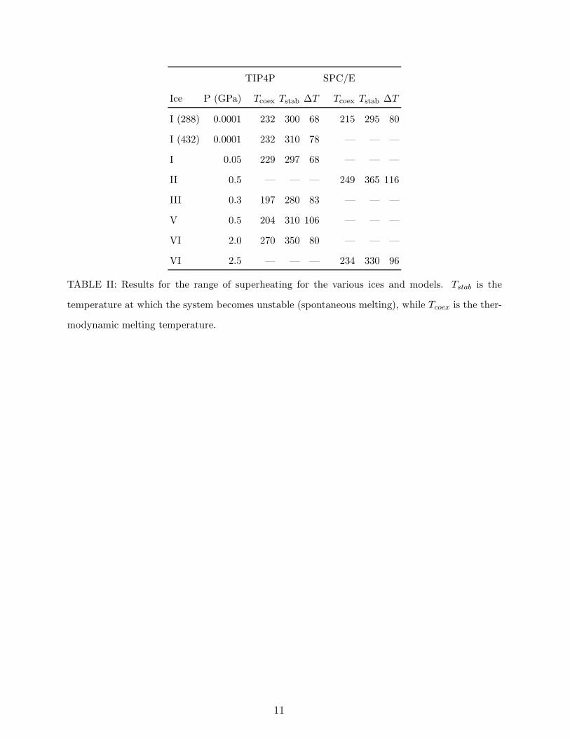
Table II presents the first temperature for which spontaneous melting of ices was found

(see the column labeled as Tstab). It should be noted that in all cases, simulation runs of up

4

to 2.4×105 cycles were performed for a lower temperature (by 5 or 10 K) without success in

melting the ice. In table II, the melting temperatures of the corresponding ice phase for the

TIP4P and SPCE models are also shown for comparison (column denoted as Tcoex). The

latter values are taken from [11] and were calculated by determining the free energies of the

fluid and solid phases. ∆T (we shall denote this value as the meta stability range) represents

the difference between Tstab and Tcoex and is also given in Table II. For ice I the stability

range depends only weakly on pressure (for the two pressures considered the range is about

∆T = 68K). The stability range of different ices of a certain model are slightly different,

although these differences are never large. For the TIP4P, we may state that 80 K is the

typical range of meta stability of the different ice phases. For the SPC/E model the meta

stability range appears to be about 90 K (i.e., 10 K larger than that of the SPC/E). This is

not surprising since the internal energies of the solids are always lower in the SPC/E model

than in the TIP4P model (the hydrogen bonding is slightly stronger in the SPC/E model

when compared with the TIP4P model). In any case, differences in the stability range of

both models (SPC/E and TIP4P) are small. In this respect, the numbers presented here

represent the typical values of the stability range that would be expected to be found in

simulations of other realistic models of water. Although a systematic study of the system

size dependence of Tstab has not been performed, we have studied the behavior of Tstab for

ice Ih of the TIP4P model at p = 0.1 MPa for two system sizes: 288 molecules and 432

molecules. The 50% increase in system size delays the onset of melting by about 10 K.

Finally, figures 2 and 3 show the location of the stability temperature (symbols) of the

different ices for both the TIP4P (figure 2) and for the SPC/E (figure 3). The phase diagram

as obtained from free energy calculations is also shown (lines). It can be seen that the degree

of superheating is of the order of 85 K. Interestingly the stability temperatures reflects the

trends found in the equilibrium coexistence lines. This suggests that a first rough estimate

of the melting temperature of ices can be obtained from the NpT simulations. Although

for the SPC/E model ice III and V (and also ice Ih!) are not thermodynamically stable

phases (i.e for any given p and T another ice always exists with lower Gibbs free energy)

they are mechanically stable and it is possible to perform simulations of these phases [11].

The stability limit has been studied only for the thermodynamically stable phases of the

TIP4P and SPC/E models. However it is also possible to determine Tstab for ices which

are metastable with respect to other solid structures. For example for ice III in the SPC/E

5

model at p = 0.5 GPa it was found that Tstab = 270 K, which is substantially lower than the

value obtained for ice II (the thermodynamically stable phase of the SPC/E at this pressure)

at the same pressure, having Tstab = 365 K.

ACKNOWLEDGMENTS

Financial support from project numbers FIS2004-06227-C02-02 and BFM-2001-1017-C03-

02 of the MCYT (Ministerio de Ciencia y Tecnologıa) is acknowledged. C.M., would like

to thank the Comunidad de Madrid for the award of a post-doctoral research grant (part

funded by the European Social Fund). E.S. would like to thank MEC for a predoctoral

grant. L.G. MacDowell would like to thank the Universidad Complutense de Madrid and

MCYT for the award of a Ramon y Cajal fellowship.

6

[1] J. A. Barker and R. O. Watts, Chem. Phys. Lett. 3, 144 (1969).

[2] A. Rahman and F. H. Stillinger, J. Chem. Phys. 55, 3336 (1971).

[3] S. C. McGrother, D. C. Williamson, and G. Jackson, J. Chem. Phys. 104, 6755 (1996).

[4] P. Bolhuis and D. Frenkel, J. Chem. Phys. 106, 666 (1997).

[5] M. R. Wilson, Molec. Phys. 85, 193 (1995).

[6] C. Vega, C. McBride, and L. MacDowell, J. Chem. Phys. 115, 4203 (2001).

[7] E. de Miguel and C. Vega, J. Chem. Phys. 117, 6313 (2002).

[8] M. R. Wilson, J. Chem. Phys. 107, 8654 (1997).

[9] G. C. Boulougouris, I. G. Economou, and D. N. Theodorou, J. Phys. Chem. B 102, 1029

(1998).

[10] L. A. Baez and P. Clancy, J. Chem. Phys. 103, 9744 (1995).

[11] E. Sanz, C. Vega, J. L. F. Abascal, and L. G. MacDowell, Phys. Rev. Lett. 92, 255701 (2004).

[12] E. Sanz, C. Vega, J. L. F. Abascal, and L. G. MacDowell, J. Chem. Phys. 121, 1165 (2004).

[13] H. J. C. Berendsen, J. R. Grigera, and T. P. Straatsma, J. Phys. Chem. 91, 6269 (1987).

[14] W. L. Jorgensen, J. Chandrasekhar, J. D. Madura, R. W. Impey, and M. L. Klein, J. Chem.

Phys. 79, 926 (1983).

[15] I. Nezbeda, J. Molec. Liq. 73, 317 (1997).

[16] A. Gil-Villegas, A. Galindo, and G. Jackson, Molec. Phys. 99, 531 (2001).

[17] A. Galindo, A. Gil-Villegas, G. Jackson, and A. N. Burgess, J. Phys. Chem. B 103, 10272

(1999).

[18] J. Janecek and T. Boublk, Phys. Chem. Chem. Phys. 5, 2391 (2003).

[19] T. Boublik, Molec. Phys. 76, 327 (1992).

[20] D. Frenkel and A. J. C. Ladd, J. Chem. Phys. 81, 3188 (1984).

[21] D. A. Kofke, J. Chem. Phys. 98, 4149 (1993).

[22] M. P. Allen and D. J. Tildesley, Computer Simulation of Liquids (Oxford University Press,

1987).

[23] G. E. Norman and V. V. Stegailov, Doklady Physics 47, 667 (2002).

[24] S.-N. Luo, A. Strachan, and D. C. Swift, J. Chem. Phys. 120, 11640 (2004).

[25] V. F. Petrenko and R. W. Whitworth, Physics of Ice (Oxford University Press, 1999).

7

[26] L. Pauling, J. Am. Chem. Soc. 57, 2680 (1935).

[27] V. Buch, P. Sandler, and J. Sadlej, J. Phys. Chem. B 102, 8641 (1998).

[28] D. Frenkel and B. Smit, Understanding Molecular Simulation (Academic Press, London, 1996).

8

Captions to the figures:

Figure 1: A plot of the intensity of the structure factor, Ihkl, for the TIP4P model

of ice V at 310 K and 0.5GPa. This plot is representative of the sudden fall in the intensity

of the structure factor associated with melting.

Figure2: Plot of the phase diagram of water for the TIP4P model. Points are the

temperatures at which the solid melted under constant pressure. � ice I (288 molecules),

� ice I (432 molecules), H ice III, � ice V, and N ice VI.

Figure 3: Plot of the phase diagram of water for the SPC/E model. Points are the

temperatures at which the solid melted under constant pressure. � ice I, • ice II, and N ice

VI.

9

Ice No. of molecules

I(Ih) 288

I(Ih) 432

II 432

III 324

V 504

VI 360

TABLE I: Relation between the number of molecules in the simulation box and the ice structure

simulated for both the SPC/E and the TIP4P models.

10

TIP4P SPC/E

Ice P (GPa) Tcoex Tstab ∆T Tcoex Tstab ∆T

I (288) 0.0001 232 300 68 215 295 80

I (432) 0.0001 232 310 78 — — —

I 0.05 229 297 68 — — —

II 0.5 — — — 249 365 116

III 0.3 197 280 83 — — —

V 0.5 204 310 106 — — —

VI 2.0 270 350 80 — — —

VI 2.5 — — — 234 330 96

TABLE II: Results for the range of superheating for the various ices and models. Tstab is the

temperature at which the system becomes unstable (spontaneous melting), while Tcoex is the ther-

modynamic melting temperature.

11

0

0.05

0.1

0.15

0.2

0.25

0.3

0.35

0.4

0.45

0.5

0 10000 20000 30000 40000 50000 60000 70000

I hlk

Monte Carlo steps

12

0.0001

0.001

0.01

0.1

1

10

100 150 200 250 300 350 400 450

Pre

ssur

e (G

Pa)

Temperature (K)

I

II

VI

VIII VII

liquid

V

III

13

0.01

0.1

1

10

100 150 200 250 300 350 400 450

Pre

ssur

e (G

Pa)

+ 0

.1

Temperature (K)

I

II

VI

VIIIVII

liquid

14