JOURNAL OF GEOPHYSICAL RESEARCH, VOL. 97, NO. Cll, PAGES 17,729-17,738, NOVEMBER 15, 1992

Sea Ice Melting and Floe Geometry in a Simple Ice-Ocean Model

MICHAEL STEELE

Polar Science Center, Applied Physics Laboratory, College of Ocean and Fishery Sciences, University of Washington, Seattle

A coupled sea ice-ocean numerical model has been developed that addresses the role of floe geometry dur- ing summertime melting. The model contains a diagnostic equation for average floe diameter in addition to the usual prognostic equations for ice volume per unit area and ice concentration. The partition between melt- ing on the top, bottom, and lateral (side) surfaces of floes is examined using time-dependent simulations with differing initial average floe diameters. The different parameterizations for bottom and lateral melting in the literature are also compared and found to vary significantly. The results show that lateral melting is important only for floes with diameters less than 0(30 m), given atmospheric thermal forcing typical of the central Arc- tic in summer. This means that the decrease in ice concentration over the summer is a strong function of floe diameter, in keeping with simple geometrical arguments. In all cases, about 80% of the net thermal energy that enters the ocean through leads goes toward melting ice, while the rest warms the ocean.

1. INTRODUCTION

The summer sea ice cover is a jumbled ensemble of floes of various sizes and shapes floating on the ocean surface. Figure 1 shows an example, a digitized photomosaic obtained during the Arctic Ice Dynamics Joint Experiment (AIDJEX) in the Beaufort Sea [Rothrock and Thorndike, 1984]. The volume of ice in a par- ticular region is usually given by the distribution function g (H), which describes the fractional cover of ice of thickness H

[Thorndike el al., 197:5]. More commonly, numerical models use two state parameters for the amount of ice in a given region: h, the "equivalent thickness" (volume of ice divided by the surface area of the region), and A, the areal concentration of ice of thick- ness greater than some threshold h0 (usually taken as 0.5 m) [Hibler, 1979, hereinafter "H79"]. These parameters are ade- quate to describe exchange processes in the air-ice-ocean system if one considers only the top and bottom surfaces of the floes. However, transfer also occurs at the edges of floes. Steele et al. [1989a], for example, discuss how lateral stresses affect floe velo- city. Similarly, floe melt rates are affected by heat transfer on the top, bottom, and lateral faces. This paper describes a numerical model that considers this heat partition for a simple case.

Consider the idealized states depicted in Figures 2a and 2b, in which the sea ice cover consists of uniform floes of a given diam- eter. The areal coverage is approximately the stone in both cases. Assume that the floe thicknesses are also identical. Now ask,

"For the same (atmospheric) thermal forcing, how will the melt rates differ for Figures 2a and 2b?" Intuitively, we expect more melting for Figure 2a because the total perimeter, or lateral sur- face area, is greater than in Figure 2b although the top and bob tom surface areas are the same. Thus the areal coverage should decrease faster for Figure 2a.

The numerical models of sea ice presently in use are unable to distinguish between the states shown in Figures 2a and 2b [e.g., H79; Melior and Kantha, 1989, hereinafter "MK89"]. These models do not contain an explicit treatment of floe geometry such as an equation for the floe diameter. Half the heat that enters tlm ocean through leads is assumed to cause a decrease in ice concen- tration, while the other half decreases ice thickness. This relation-

ship is fixed for all time in these models. In the model described here, the melt rates on the top, bottom,

and lateral floe surfaces are calculated independently. The heat

Copyright 1992 by the American Geophysical Union.

Paper number 92JC01755. 0148-0227/92/92JC-01755505.00

balances on each ice surface are computed using the observations and models of Maykut and Perovich [1987] (hereinafter "MP87") on the heat budget of summer leads. The role of the molecular sublayer at the ice-ocean interface [McPhee et al., 1987] is also included. For leads less than several hundred meters wide, MP87 found that the total melt rate, as well as the

partition between top, bottom, and lateral melting, depended on the initial width of the lead. Their results were expressed in terms of the growth rate of a single lead's width during a period of solar heating. With a view toward larger-scale modeling, the results here are expressed in terms of an ensemble of floes that experience changes in thickness and diameter. In this context we ask the question, "How important is lateral melting in the overall melt rate of the sea ice cover?"

The equations for the ice and ocean models are discussed in section 2, along with the heat, salt, and momentum coupling between the models. The numerical simulations and their results

are presented in section 3. Section 4 contains a discussion of the results.

2. THEORY

2.1. Sea Ice Model

To estimate the partition of fluxes between top, bottom, and lateral ice floe surfaces, we need to know the relative amount of

each type of surface area. The first step is to find a horizontal length scale for a floe that can be related to these surface areas. Following Rothrock and Thorndike [1984], we define the "mean caliper diameter" L as the average over all angles of the distance between two parallel lines (or calipers) that are set against the floe's sidewalls. For a circle, L is the diameter as usually defined; for a square, L is intermediate between the length of a side and the diagonal.

The top surface area of each floe will be referred to as the "horizontal surface area" (equal to the bottom surface area), in contrast to the "lateral surface area" around the sides of the floe.

The concept of mean caliper diameter allows us to use the gen- eral result that

p =nL (1)

for any convex shape, where p is the perimeter. RotMock and Thorndike found that for Figure 1 the ratio p/L had a mean of 3.17 and standard deviation of only 0.04; i.e., floes were largely convex. Note, however, that the smallest floes they digitized from the photomosaic were approximately 1 km in diameter. It is assumed in this paper that the geometrical properties found by

17,729

17,730 STEELE: SEA ICE MELTING AND FLOE GEOMETRY

Rothrock and Thorndike for Figure 1 extend to smaller scales. This seems reasonable considering their discussion of the scale invariance of floe geometry (see their Figure 4), but also suggests the need for further observations.

Unfortunately, there is no simple relation like (1) for s, the horizontal surface area. Rothrock and Thorndike found that

s =aL 2 (2)

where the mean value of ot = 0.66 (and standard devia- tion = 0.05). This is the value used here; sensitivity experiments are discussed in section 3.

If we assume that melting occurs uniformly at a rate W ia t around the perimeter of the flow,

ds - WlatP (3)

dt

Substituting from (1) and (2) then gives

dt 2o•

km

IO0

80

60

40

--w•at (4) 20

which relates the loss of average floe diameter dL/dt to the sidewall melt rate w]at.

We now turn our attention from the geometry of single floes to parameters that describe an ensemble of such floes in a given region. The areal concentration a is the ratio of ice-covered hor- izontal area containing n floes of a particular diameter to the total horizontal surface area Stot in a region; i.e.,

a = (5) s tot

The total concentration A is the sum. of a over all diameters. For a region containing floes with only a single diameter L,

A = --n--ns(L) (6a) S tot

n• 2 (6b) tot

Ao L2

A- Lø • (6c) where the subscript "0" in (6c) refers to the initial condition and n is assumed to be constant. The analogous quantity for the ratio of lateral surface area to total horizontal surface area is

At. = A r•H /otL, where H is the ice thickness. In this paper, the sea ice cover is assumed to be well described

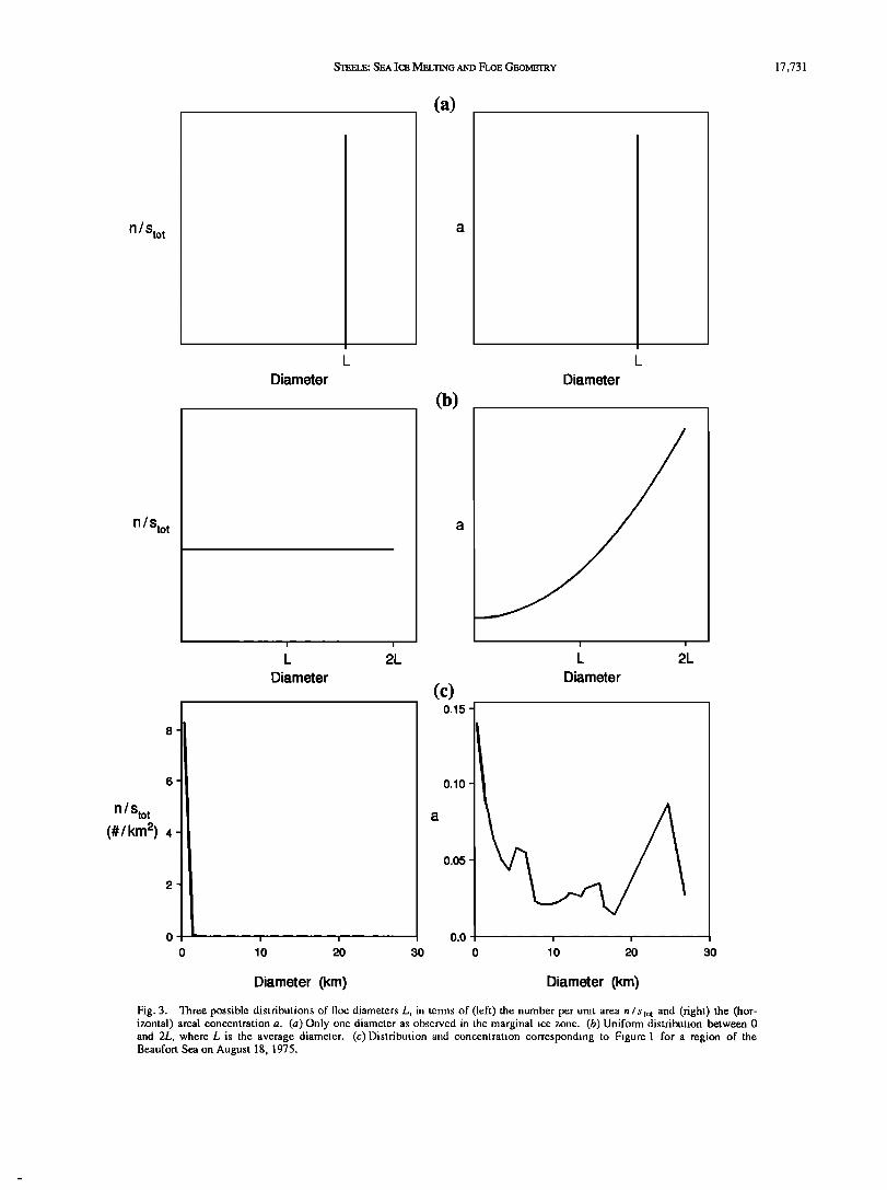
by a single "average diameter." Figure 3 illustrates several pos- sible distributions of n/Stot with respect to floe diameter. In Figure 3a a delta function at L represents a field of floes with identical diameters, such as observed in parts of the marginal ice zone (MIZ) [Wadhams et al., 1988]. Figure 3b illustrates a uni- form distribution of diameters from 0m to twice the average value L. This is analogous to the distribution assumed by H79 for ice thickness during melting. In this case, concentration a varies as the square of diameter. Figure 3c shows the distribution that corresponds to Figure 1; for this plot, the floes in Figure 1 were digitized down to about 30 m diameter (D. A. Rothrock, personal communication, 1992). This distribution is a strong function of diameter; i.e., there are many more small floes than large ones; in this case, ice concentration a is a weakly decreasing function of

60 80 100 120 140 krn

Fig. 1. Digitized floe boundaries from a mosaic of aerial photographs of summer pack ice in the Beaufort Sea [Rothrock and Thorndike, 1984].

100 km

(a)

L1 << L2

(b)

Fig. 2. An idealized pair of sea ice states (plan view). Solar heating of the ice-ocean system leads to a different response for each state, depend- ing on the total ice floe perimeter. Standard numerical models cannot differentiate between states (a)and (b).

diameter. The concept of "average diameter" is most obviously applicable to Figures 3a and 3b. An average diameter may, of course, also be defined for Figure 3c, but it is not sufficient to describe the distribution completely [Rothrock and Thorndike, 1984]. The applicability of the present model to this case is dis- cussed further in section 3.

We consider here the changes in the sea ice state due to melt- ing only. When other processes such as advection, internal ice stress, and freezing are neglected, the prognostic equations for sea ice volume AH and total concentration A in a given region

and

reH (AH) = A [wtq, + Wt,ot + '•-w]•, ] (7)

dA nH

H '•- =A -•- w,,.t (8)

STEELE: SEA ICE MELTING AND FLOE GEOMETRY 17,731

(a)

n / Sto t

L L

Diameter Diameter

n/Stot

8

6

n/Sto t (#/km 2) 4

2

0 ,

0 10

I I I I

L 2L L 2L

Diameter Diameter

(c)

i

20 30

0.15

0.10

0.05

0.0

0 10 20 30

Diameter (km) Diameter (km)

Fig. 3. Three possible distributions of floe diameters L, in terms of (left) the number per unit area n / $tot and (right) the (hor- izontal) areal concentration a. (a)Only one diameter as observed in the marginal ice zone. (b) Uniform distribution between 0 and 2L, where L is the average diameter. (c) Distribution and concentration corresponding to Figure 1 for a region of the Beaufort Sea on August 18, 1975.

17,732 STEELE: SEA ICE MELTING AND FLOE GEOMETRY

where w is the melt rate on each ice surface. Figure 4 illustrates the heat and salt fluxes (described below) associated with each melt rate. Note that in (7) the role of lateral melting is negligible for rcH/ct.L < < 1; i.e., large floes melt mostly from top and bot- tom surfaces and produce little change in areal concentration. Equation (8) follows from differentiation of (6a) with respect to time and substitution from (1), (3), and (6b). The main difference between prognostic equations (7) and (8) and those used in models such as H79's and MK89's without an explicit treatment of floe geometry is in the lateral melting terms. Instead of the w•.• t term, those models use an expression that is proportional to the total heat flux at the ocean surface. MK89 partition this flux equally between sink terms for ice thickness and ice concentra- tion via their parameter (I) m, to which their results were fairly sensitive. H79 assumes a uniform distribution of ice thicknesses during melting, which leads to sink terms similar (although not identical) to those of MK89. This assumption can be compared with the rather complex seasonal thickness distributions observed in the Arctic by Bourke and Garrett [ 1987].

I Ftop • .. / lead I' fi•.w,. , •

\\ • • Glat Gbot _•...• • • '---"---*----•-• G tø P •.,..'"• ocean • • model

levels

Z n ----

Fig. 4. Heat fluxes F and salt fluxes G in the ice-ocean model defined in the text. The heat (salt) flux is positive (negative) in the direction of the arrows. The air-water heat flux F•,• is a function of depth (denoted by dashed arrow) because of subsurface absorption of shortwave radiation. The numerical grid is also shown. qhe first level of the model lies below the ice bottom; i.e., we assume that the water above this point is Uni- formly well mixed.

Following MP87, the conductive heat flux through the ice is neglected in the "high summer" simulations discussed here. This means that the ice surface melt rate w to P is proportional to the net air-ice heat flux Fro p via wt,,p = -Ftop/PiQ, where Pi is ice density (= 910 kg m -3) and Q is the latent heat of fusion for sea ice. The latter quantity is a moderate function of' the ice salinity [McPhee and Untersteiner, 1982], which varies with depth in thick ice. In the interest of simplicity, we use a fixed value of Q = 2.92 x 105 J kg -•, which corresponds to an ice salinity of 4 psu. The surface flux Fro p is a combination of sensi- ble, latent, and radiative contributions. We use the parameteriza- tions of MP87 and the constants appropriate for their "cloudy, central Arctic" case, with the following exceptions. The incom- ing shortwave flux and surface air temperature are taken as the average values of the July and August observations by May/cut

[1982], or 181.75W m -2 and-IøC, respectively; these values remain constant with respect to time over the integration. Also, a fixed wind speed of 6 m s -• is used in the turbulent flux formulas. The ice albedo for ice thicker than 1.1 m is set to 0.64, which is the value for July used by Maykut and Untersteiner [1971] in their study of multiyear ice. The albedo decreases as the ice thins, in accord with the formula of Perovich [1983], down to a value of 0.48 at H = 0.2 m. Also, the ice temperature is set to -1 øC. The decrease in ice thickness AH over a time step At due to surface melting is given by AH = TAt Wtop, where Tis the frac- tion of surface melt that is lost to runoff. (The rest remains on the surface as melt ponds and refreezes in the fall.) Following May- /cut and Untersteiner [1971], we set T = 0.5.

Similarly, the ice bottom melt rate w t,,,t is proportional to the ice-water heat flux at the ice bottom via w•,t = -F•,t / PiQ. The flux Fbot is found by solving a system of ice-ocean boundary equations as described by Mellor et al. [1986], McPhee et al. [1987], and Steele et al. [1989b]. The solution assumes the existence of a molecular sublayer at the rough ice-ocean interface in which turbulent exchange is suppressed and molecular diffusion is dominant. The resulting melt rates for a given water temperature are reduced relative to the fully turbulent case. A simpler parameterization for bottom melting described by McPhee [1992] was also tested and yielded results similar to the full boundary layer solution.

The ice lateral melt rate w• t is likewise proportional to the ice-water heat flux at floe edges via w•.•t = -Flat / piQ. However, this process is poorly understood in comparison with bottom melting. Several parameterizations for lateral melting are com- pared in Table 1. The table also shows the molecular sublayer formula used for bottom melting, which is based on laboratory experiments and has been tested both in the field [McPhee et al., 1987] and in numerical models tRiedlinger and Warn-Varnas, 1990]. Table 1 shows that the simple McPhee [1992] formula produces results that are very similar to the full sublayer solution. The laboratory experiments of Josberger and Martin [1981] predict an order of magnitude less ablation than that given by the molecular sublayer formula. The Perovich [1983] model predicts lateral melt rates that are quite close to those of the molecular sublayer formula, and the MP87 formula predicts melt rates that are about 2.5 times stronger.

It is not immediately obvious how lateral melting relates to bottom melting. However, the fresh, buoyant meltwater behaves

TABLE 1. Lateral and Bottom Melt Parameterizations

Sample Value, Reference Melt Rate Formula cm d -•

Josberger and Martin [ 1981 ] Wl•t m • AT m3 0.28

Perovich [1983] wt•t m2AT m3 1.55

Maykut and Perovich [ 1987] W•at m • u• AT m4 4.61 1

Steele et al. [1989a] Wbo t •TT UXAT/Q ' 1.78 McPhee [1992] Wbot cnu•aT/Q' 1.59

Parameterizations depend on the elevation of the water temperature above the freezing point, AT, and the skin friction velocity ux, which in the final column are set to 0.2øC and 1 cm s -• , respectively. The first for- mula for lateral melting and the first for bottom melting are from labora- tory experiments; the others are from field data. The empirical constants (m•, m2)= (0.3, 1.6)x 10 -6, (m3, m4)= (1.36, 1.30), and ch = 0.0058. The normalized latent heat is defined as Q '-- rQ / c•, where r = 0.9 is the ratio of ice to water density and c• = 4218 J kg -• øC-• is the heat capa- city of water. The molecular sublayer factor 1/AT is a function of the sub- layer Reynolds and Prandtl numbers [Steele et al., 1989a].

STEELE: SEA ICE MELTING AND FLOE GEOMETRY 17,733

very differently in the two situations. During lateral melting, the more buoyant meltwater will rise along the vertical ice-water interface, allowing new, warm water to influence the ice. During bottom melting, the melt water is trapped at the horizontal ice- water interface; this trapping can be enhanced by the under-ice topography. Thus it seems reasonable to expect that lateral melt rates may be larger than bottom melt rates for the same thermal forcing. The additional effect of relative ice-ocean motion would tend to increase the flushing rate on both surfaces. In the simula- tions discussed in section 3, we compare results obtained by using (l) Wla t : Wbot, where Wbot is given by the molecular sublayer, and (2) Wlat as given by the formula of MP87.

Like MP87, we assume that lateral melting occurs uniformly over the entire lateral face of the ice lloes (which we distribute over the thickness H, not just the draft D = pill / Pw, where p•, is the water density). This will be true only k)r thermally well mixed leads, which, the observations of MP87 aside, may be more of a numerical convenience than a physical reality.

In summary, the sea ice equations of state comprise (7) and (8), which are prognostic equations for AH and A, along with the diagnostic equation (6c) for L. The thickness H is obtained by subtracting (8) from (7).

2.2. Ocean Model

The equations for ocean current u, temperature 7; and salinity S are

at -i + Tzz (9a)

aT 3 [ aT at - 3z Kh 3--7- + F,,•/p•c• (9b)

3t - 3z Kh • (9c)

where c•, = 4218 J kg -1 øC-1 is the heat capacity of water. The current is given in complex notation as u = (ux, iuy) and is com- puted only in order to obtain values for K,,, and Kh. The latter are the viscosity and diffusivity coefficients, respectively, and are composed of turbulent and molecular contributions. The molecu- lar effects become important only at the ice-ocean interface, as discussed by Steele et al. [1989a]. The turbulent coefficients are obtained via the level 2.5 turbulence-closure scheme of Mellor

and Yamada [1982]. The procedure involves solving prognostic equations for the turbulent kinetic energy and turbulent length scale. This results in K,,, and K h that are functions of both depth and time (see Steele et al. [1989a] and Meltor and Yamada [1982] for details). An alternate method was also tested in which K,, and Kh were functions only of the surface stress [Steele et al., 1989b], but this yielded unrealistically deep mixing in the pres- ence of stabilizing melt fluxes. The Coriolis parameter is f = 1.43 x 10 -'• s -1 , corresponding to a latitude of 80 ø.

The flux of shortwave energy that penetrates through the ice and into the leads is given by F•,. The part penetrating the ice has been neglected in these simulations, since it is less than 1% of the flux predicted at the ice top surface when using the MP87 parameterization for 2- to 3-m-thick ice. The flux in the lead is a function of depth, with the surface value given by F•,,,(0)= (1- ot•,)F•, where eta, = 0.1 is the water albedo and F• is the incoming shortwave flux (= 181.75 W m-2). The flux at levels below the surface is reduced by a logarithmic factor given by

MP87 for cloudy, central Arctic conditions. The flux at 3-m depth, for example, is about 38% of the surface value. Sensi- tivity studies showed that if the shortwave flux was assumed to occur only at the surface, melt rates were enhanced by about 10% and warming of the ocean column was reduced by about 35%.

2.3. Ocean Surface Boundary Conditions

The ocean surface stress is fixed at 0.1 N m -2 for all time, since we are not concerned here with the details of the momentum

transfer between air, ice, and water.

The ocean surface heat flux F.,.•r is given by

Fsurf= [(1-A)Fa,,, ] +A (10)

where F aw is the net air-water heat flux in leads (including the shortwave flux F•,,,(0)), as given by the parameterizations of MP87 with the modifications described previously. The shortwave flux dominates the air-water heat balance. Tile ice

bottom and lateral fluxes Fbo t and Fla t have been described previ- ously. All of these fluxes are illustrated in Figtire 4. The first term on the right-hand side of (10) represents the heat source for the ocean surface, and the terms in the second set of square brackets represent the heat sinks. Ocean heating restilts when the rate at which heat is input to the ocean surface is greater than the rate at which heat is lost as ice melts.

The ocean surface salt flux G •=f is given by

G,o•f = A G top + G hot + q.L lat (11 )

where G to p is the salt flux associated with runoff from the ice top surface, and Cbo t and Sla t are the salt fluxes associated with ice melting on the bottom and lateral surfaces, respectively. These fluxes are shown in Figure 4. Each of the ternas on the right-hand side of (11) represents a freshwater flux to the ocean during the summer melt season.

The fluxes on the right-hand side of (11) are given by Gj = 10-3piTjASwi, where j = (top, bot, lat), Tj = (0.5, 1, 1), and AS --S1 -Si. The salinities S• and Si are defined as those at the uppermost grid point of the ocean model and in the sea ice, respectively. We set the latter to 4 psu. The density of sea ice Pi is 910kgm -3. The factor ?• = 0.5 accounts for runoff, as described previously. The units of salt flux are kilograms of salt per meter squared per second; fluxes are negative when ice melts.

2.4. Numerical Scheme

The numerical simulations assume horizontal homogeneity; thus the grid consists simply of 60 depth levels down to 100 m, which is deeper than the neutral Ekman layer depth for the given 0.1 N m -2 surface stress. Ocean properties (currents, tempera- ture, and salinity) are staggered with respect to their fluxes (including the turbulence quantities such as the viscosity and diffusion coefficients K,,, and Kh). The flux grid starts at a depth below the surface equal to the ice draft D plus the average sea ice roughness length z0 (0.06 m) and increases in spacing exponen- tially fi'om 0.01 m to 12 m (at the bottom). The property grid is defined at the midpoints of the flux grid. The integration is car- ried out for 60 simulation days, with a 30-min time step. Figure 4 illustrates the grid spacing in relation to the lead. We implicitly assume in this model that the water in the lead is homogeneous and is in fact well mixed with the water just under the ice bottom.

17,734 STEELE: SEA ICE MELTING AND FLOE GEOMETRY

3. EXI)ERIMENrI'S AND RESULTS

The following numerical simulations are designed to simulate the decay of the sea ice cover during the height of the arctic sum- mer. The simulations are run for 60 days corresponding to the months of July and August. The initial ice cover is specified as having an areal concentration of 90% and a thickness of 3 m. The initial floe diameter L0 varies. The initial ocean state is quiescent, with a uniform salinity of 32 psu and a temperattire at the freezing point. Motion is induced by linearly ramping tip the ocean surface stress over the first inertial period, which reduces inertial ringing. The thermal forcing is similarly ramped tip from inertial period 3 to period 4.

Each set of simulations described here consists of three cases, defined by an initial average floe diameter L0 of 30 m, 300 m, and 3000 m. The geometrical factor •H/q/., (equations (7) and (8)) for these cases is 0.476, 0.048, and 0.005, respectively. As a control, an additional simulation was performed in which lateral melting was not allowed, so that only ice thickness changed with time.

In the simulations, wl• t was given by either (1) the formula of MP87 (Table 1), or (2) Wbot using the moleculm' sublayer lbr- mula. Results are shown only [br the former case. This is because changes in the thickness of the top and bottom surfaces were similar in both cases. Changes in floe diameter and concentration were not similar, however; the changes predicted for case 2 (wl,•t = Wbot) can be obtained from (4) and (6c), respectively, given the change in thickness due to bottom melting.

Figure 5 shows the change in sea ice state parameters as a function of time. The change in ice concentration is a strong function of L0. This is analogous to Figure 8 of MP87, in which the change in ice concentration is a strong function of the initial lead width. Thickness changes are partitioned aLx)ut equally between bottom and top melting (which means that the top melt- ing rate is actually twice as fast as tile bottom when the factor T is taken into account; see section 2.1). Average values of dL/dt in Figure 5 are 1.7 cm d -1, which corresponds to wl,•t = 0.7 cm ct -1 using (4). That is, the rate at which a floe melts back laterally at any point along its perimeter is generally less than a centimeter per day. MP87 and Ilall and Rolhrock [1987] observed a variety of lateral melt rates in the warm (generally greater than 0øC) water of the MIZ, including short periods with rates as high as 40 cm d -1 . Melt rates were generally less than 10 cm d -1, how- ever.

When w•.• t is set equal to w•,t, the changes in thickness are similar to those shown in Figure 5, with the same equal partition between top and bottom melting. On the other hand, tile decrease in floe diameter at 60 days is less, about 0.5 m for all initial L0' the decrease in concentration is (0.0286, 0.0029, 0.0003) for L0 = (30, 300, 3000)m. These values may also be derived simply from (4) and (6c), given that the floes melt about 0.2 m from the bottom in all cases.

The geometrical factor IcH/0:L gives the ratio between lateral and horizontal ice surface area. Sensitivity studies were run with 0:=0.785 (perfectly circular floes) and with 0:=0.463 (3 x 1 rec- tangular floes). The rate of concentration decrease is an inverse function of 0: via (8); however, the difference in ice concentration at 60 days between the two cases was only about 0.01 for L0 = 30 m. Qualitatively, we expect that, in the absence of mechanical forcing, ice floes would become more circular as the 5 , melt and the rate of concentration decrease would slow down.

Figure 6 shows the oceanic response in terms of the tempera- ture and salinity of the mixed layer. There is a layer of warmer, fresher water about 20 m deep embedded within the uniform ini- tial ocean state which is produced by aunospheric heating and the

0.92

0.90

0.88

=o

• 086 (D '

0 o

0.84

0.82

0.80

, I I I i I

Lo = 3000 rn ',

Lo = 300 rn --

--

............ Lo = 30 rn

dL/dt = 0 i i ! !

0 10 20 30 40 50 60

(a)

3.0 -

2.2 -

2.0

-2

-3

I I I I I

Lo = 3000 rn

Lo = 300 rn

............ Lo = 30 rn

dL/dt = 0

I I I I I

0 10 20 30 40 50 I I I I i

.............. _ ............... _

Lo = 3000 rn

- Lo = 300 rn _

............ Lo = 30 rn

dL/dt = 0

I I I I m

0 10 20 30 40 50 60

(b)

(c)

time (days)

Fig. 5. Temporal changes in (a) ice concentration, (b) ice thickness, and (c) floe diameter. The ice concentration decreases most dramatically for small floes.

resulting ice melting. Its depth is defined here as the level at which the turbulent kinetic energy is reduced to 10% of its sur- face value [Martin, 1985]. Note from Figure 6 that the mixed layer is coldest and freshest when L0 = 30m. More melting occurs here than in the other cases because of the larger amount of ice-ocean interface.

S•E: SE^ IC• MELTING AND FLOE GEOMETRY 17,735

-1.4

-1.8

0

I I

Lo = 3000 m

Lo = 300 m

Lo = 30 m

dL/dt= 0

I I

(a)

I I I I I

10 20 30 40 50 60

32.1 • • I I (b) ..... Lo = 3000 m

32.0 - Lo = 300 rn _

• ............ Lo -- 30 m •_ 31.9 dL/dt=O

.• 31.8

.•_

-• 31.6 " '-

.x_

• 31.5

31.4

31.3 i i • • ,

0 10 20 30 40 50 60

time (days)

Fig. 6. Temporal changes in (a) temperature and (b) salinity of the oce- anic mixed layer. Atmospheric heating and resuhing ice inching lead to a relatively warm, fresh mixed layer.

Let us now consider the heat and salt budgets in the ocean. Using (10) and integrating (9b) over the depth of our domain, we obtain

rcH

(1 -A )f(O) = •'-A(wt, o, + •-wlat) (12)

where, following the notation of MK89 and H79, f(0)-- Fa,(O)/piQ, where F**(0) is the air-water heat flux at the ocean surface. The temporal change in the heat content of the water column, divided by the factor piQ, is given by •. Note that the heat flux at the bottom of the numerical domain (100 m depth) is set to zero. We see from (12) that the total heating contributes to three processes: ocean warming, bottom melting, and lateral melting. Figures 7b and 8b compare these processes for initial floe diameters of 30 m and 300 m, normalized by the total heat- ing. Figures 7a and 8a show the total heating, given by the left- hand side of (12), which increases with time as A decreases owing to lateral melting. Figures 7c and 8c show the freshwater fluxes due to melting from top, bottom, and lateral ice surfaces, normalized by the total at each time step.

Lateral melting plays a major role only for the smaller floes. Approximately 20% of the net forcing goes into warming the ocean. (This is reduced to about 10% when the shortwave flux is assumed to occur only at the ocean surface.) This result is in con- trast to many ocean models which assume that the ocean remains at the freezing point as long as ice exists in the domain (i.e., /•, =- 0 for all time). Also note that, for larger floes, the freshwater fluxes (Figures 7c and 8c) are about equally distributed between top and bottom melting.

To examine these issues further, we divide (12) by the left- hand side (1 -A )f (0) to obtain two nondimensional quantities,

A w bot A I'I bot (I)•ot = (1 - A)f (0) = (1 - A )f (0) (13a)

and

A L W lat tl, l•t (1 -A)f(O) (1 -A)f(O) (13b)

where tl)bot and (•lat are the fraction of incoming heat at the ocean surface that is used in bottom and lateral melting, respectively. The lateral surface concentration At. was defined just after (6). The second equalities in (13a) and (13b) use (7) and (8), where the dot indicates time rate of change. The results are plotted in Figure 9 for the same L0 shown in Figures 7 and 8. Note that 4)v.t is equivalent to the parameter (I),,, of MK89. In lieu of an explicit parameterization for ice floe geometry such as presented here, the MK89 and H79 models assign a fixed value of tl)bot = (1)•t = 0.5 (considering only the part of their versions of (7) and (8) that depends on atmospheric heat flux f (0)). For comparison, the value (I) = 0.5 is plotted in Figure 9. The partition is about 50:50 only for the smallest floes. For larger 11oes, much more heat is lost via bottom melting than via lateral melting because of the relative amounts of horizontal and lateral surface areas.

Because MP87 included no explicit ocean model, they neces- sarily defined a constant R that described the percentage of heat in the water column that returns to the ice bottom per unit time. In terms of (12), R -=-Awbo t / E. The R values calculated for the present simulation are shown in Figure 10 in units of percent per day for wv, t given by the MP87 parameterization. The results are similar when Wl, t is given by the molecular sublayer formula. MP87 used R = 50% d -• . The model discussed here indicates that MP87 overestimated the rate at which oceanic heat is transferred

to the ice bottom; McPhee et al. [1987] also found this to be the case when the molecular sublayer was neglected. In fact, a sim- ple estimate for R is easily obtained using the McPhee [1992] parameterization (Table 1) for Fbot ( = piQwb,,t ),

AChtt x R-

MLDr (14)

where the heat in the water colunto E/piQ has been parameter- ized for the sake of this argument as nonzero only within a ther- mal mixed layer MLDr. (This is deeper than the usual mixed layer owing to subsurface absorption of shortwave energy.) For A=0.9, cn =0.0058, ux=0.01ms -•, and MLDr=40m, R= 11%d -• .

4. D•SCUSS•ON

We return now to our original question: "How important is lateral melting in the total volume melted from sea ice floes?" Figure 11 shows the melting from top, bottom, and lateral sur- faces over the 60-day integrations. Lateral melting is important

Ocean heating 40 I I I I I .

a

30- _

x 20- _

10- _

0 - I I I I I

0 10 20 30 40 50 60

time (Days)

Thermal response (normalized)

Ocean warming b

0.4

t"'"" "':' :". ß ß ß ß ß A.' "• i••._.:ii•i ................. •':'='=•':•:•.,•i:...':•i r- '"'-"ii' ';. ß ß ß . .• :;:•,' :.;:•:_;:! .....

•?• •f iii !il iii •ii•;..."i:: .................. •:•:•!•••'.."i!i ß :.: •._-• , '.: ,.: _• •:_•'.;:; ,.-...-..-.-.-.-.-•;.;o;.;.;.-..;.;.;.;,

0.0 • ...... 0 10 20 30 40 50 60

time (Days)

Freshwater fluxes (normalized)

c

0.8 Runoff

0.4-

0.2 - .:i:i::'"' ,•

0.0 • , , , • 0 10 20 30 40 50 60

time (Days)

Fig. '7. Ocean heat and salt budgets œor initial floe diameter L0 = 30 m. (a) Total heating, which increases with time as ice concentration decreases. (b) 'lTlcrmal response normalized by the iota! input i'rom Figure ?• and stocked vertically to sum to •.0. Ocean wan•in8 takes a•ut 20% o[ the incomJn• cncr•y, and lateral meldn• a•ut 50%. (c) Freshwater fluxes due to top, bouom, and lateral mclfin• normalized by the total at each dmc.

Ocean heating 40 I I I I I

30- -

E

x 20- -

10- _

0 - I I I I I

0 10 20 30 40 50 60

time (Days)

Thermal response (normalized)

Ocean warming b

0.8 - •,,--::-•.: :'• ;-..' .-•..•:= A¾..:_...-:.• ..'•...-•...::• - j,.. --...• _.•_.• ..••••• .•-- .• • ._-•••,,•,__. ,,••...•• / .•'•'*•"•.....•"•.•.•........•.•.•.•.•.•.•.•.•.•`.`••:••••........:..i•i ß ::::::::::.' ............. -.-.-.-.- - - O. 6 - ..:.:.:.. ...... -' '-'- -'-'-'-'- -'--- -' ß ß ß ß ß '-'-.---.-.-.-.-.-.-•;'•.;.•:;•.••:.;•:-_.,,

• ..:•i• ................................................ •:':•:••i••...'_i..'_.ii '• ... '-.'..-:--.'___,_.'::•_.'_,:•.'.,- ............ ', .......... '-'-'-'-••'•'.'.•..'.•.•••...':•'-'.•'•'-•.',:.x•:•:•: •- / •" ....................... -"'"'"''' ' -•'"'"'""•"'"•: '"'-•-'ø-'-"•':•::••._."iiil ß .-.-.-. ........... ._._ _ _ _•.._._._._._._._._._•;.;.;.•.;.;•..._;..•._.•:• 0.4-

./•'"""-'-'-'-'-•'"'"'•':':••••:.'..• Bottom melt '"'-'-'-'-•"-'•'•:':•::••i•iii:--"i liE" ............. - ......... •'-"- ............... -'-•'"":•:•••:•-;i:-..'•i • ............ :....,-.-...-_-.-.-.-.---------------•.,.-.-.-.-.-.-.-.-.-•,.:.,•••:••••! •. ....................................................... . .,:_._.___._._..-.•.,.,..-.•:•.•t•...•.-.:iiii •' ................... -'-'-'-'-'-'-'-'-'-'-'-'-'- - - - - - •- - - - - - -•'-'-'-'-'-'-'-'-'-'-•'"'"•.':•'•i..•i.',: O. 2 ,._:::::_.:,:,: ........... -.-m-.-.-.-.-.-.,-m-.-.- - - - - - - - - - -•.-.-.-•:-.-.-.-.-.-•;.;.;.•;•.;•.;:.;::....;.. -- '• :;_.-•:_•:• .•_;:_;:_;•,• ' ' ' ' ' ' ' ' ' ' ' ' ' ' ' ' ' ' ' ß ' ' ' ' '•.'.'.'.'.'."."."."•:.:.:•:•::::::::.;.' jl•,...............• ............. :.-.-•.,:.:..:•:.....:••..:.....-:• ......... ., .............. ,.-.....,.•••:•.-_,:_,:_,: --'""•"•-•. ............................. •;----------•'-'-"-'-'-'-'-'-'-•'""•..:..•':.••::•..'i

•,•,,-•m-,-,- .......... -.•-.-.-.-.-.-.;.-.••.;.:.•:;:.•:•._-• ,'- -, ,•_q,:.',,•-,-,• ,.•,j•,:•...•. •,,:.•,:_,•:_.'.•

•,•'•' '• ............. .'• ....... • .... 0.0 '•-'-'-'-'-'-';'•--'" ..... '- .... :;' .... • ..... •-•';'-'-'-•-q'•'-•'•'••':;•:'"-;::'";,•

I I I I I

0 10 20 30 40 50 60 time (Days)

Freshwater fluxes (normalized)

c

0.8- _

Runoff

0.6- _ x

• . . .: ! ! .• ! . . .-.-.-.-.-.-.-.;.'.'

• •i::i:: Late•ai melt u) ::::::::::::::::::::::::::::::::::: .... "'"'"""'"" ' ' ' •., '•.......j•,....j --

, .-.-.-.-.-.-.•;.;.;•;:•.:•:;:..;::....: 0.2 - '-'""•'"'•'•'••.•.•.;::'.'.;:

•..;.;:;•;•..., .-..;:.;:.;:.; ........ .... -.-.-.-.-.-.-... •,. ,.;.;.;.•:;_ _ _ _ _ _ ..;..;:;:;:;:

•..............•:.:.•::•...•:.•..• ....... .-.-.-, -..-.-._._._._.....•...;••:;:.•..;...:. ;..;:•

r'"""'"'"" """' '-'-'--------"'"'""'"'"'"" '-'•'-'•'•••"•••••••'.._•.'.:•.; o. o •"'"'•'••••.•.•i ........................... ' ' , '; ........... 'i" :*:'" :'"':':

0 10 20 30 40 50 60 time (Days)

Fig. 8. Same as Figure7, but for initial floe diameter L0 = 30Ore. Lateral melting is much less signi ticant than in Figure 7.

STEELE: SEA ICE MELTING AND FLOE GEOMETRY 17,737

(a) ............... Lo = 30 rn

Lo = 300 rn

0.8 - - ...... Lo = 3000 rn

0.6 - -

0.4 - :

;

0.2 - : -

/ .,.....,... __..,.....,.. ...........

0.0 --- ' -'•--' , , , ,

0 10 20 30 40 50 60

Z;' i'

- ..,.... ........ - ........ • ............ ..,...........,,, ......

_ - .............. Lo = 30 m .

Lo = 300 m

Lo = 3000 m ,

I I I I I

(b)

0.8

0.6

o

0.4

0.2

0.0

0 10 20 30 40 50 60

Time (days)

Fig. 9. The fraction of incoming heat at the ocean surface that goes (a) to lateral melting (el)]at) and (b)to bottom melting (tl•,,t). For com- parison, the value used by many ice-ocean models is plotted at 0.5. The partition between lateral and bottom melting is a strong function of floe diameter.

only for L0 = 30 m. (It was even less when the molecular sub- layer parameterization was used for w]at, not shown.) Top surface melting is roughly equal to bottom surface melting for the larger floes, although this is sensitive to the runoff factor T. (When ? = 0 following MP87, top melting is atx•ut twice bottom melting, in accord with the results shown in their Table 3.) The total amount of ice melted in each case is an inverse function of the initial floe diameter.

Figure 5 showed that the change in ice concentration A over the 60-day simulation was a strong function of L0, the initial average floe diameter. A field of uniformly small floes, such as can be observed in the MIZ, will melt faster (with restyect to a decrease in A) than one of large floes. This also applies to a uni- form distribution of floe sizes (Figure 3b), where L0 is taken to mean the initial average diameter. Note that the atmospheric thermal forcing used here was typical of conditions in the central Arctic; in the MIZ, the atmospheric forcing will be stronger and will be enhanced by the presence of warm ocean currents.

2O

18 -

16

14

12

v

n- 8

6

4

I I I I I

I Lo • 3000 rT1 Lo = 300 m -

............ Lo = 30 m • dlddt = 0

I I I I I 0 10 20 30 40 50 60

time (days) Fig. 10. The percent of thermal energy in the ocean that is lost to ice bottom melting per day, R. The molecular sublayer slows down this pro- cess relative to a fully turbulent simulation.

lOO

80 -

60 -

40 -

20 -

Top

........ Bottom

Lateral

I I I

I I I I

1.0 1.5 2.0 2.5 3.0 3.5 4.0

log 10 (initial diameter)

Fig. 11. The percent of inching from each ice floe surface (top, bottom, and lateral) that occurs over the course of the 60-day simulation as a function of initial diameter. Surface mehing is strongest, followed by bottom and then lateral melting for all but the smallest floes. qhe total melting during each simulation can be expressed in terms of the change in ice volume per unit area A(tlA) over the 60-day integration. For initial floe diameters L0 of 30 m, 300 m, and 3000 m, these are 0.54 m, 0.47 m, and 0.42 m, respectively. More total melting occurs when Iloes are small.

In the distribution calculated from Figtire 1 for a region in the Beaufort Sea (Figure 3c), there were many more small floes than large floes; however, the concentration of floes with diameters from 30 m to 300 m is only about 5%. Thus the change in total concentration A due to lateral melting would be small, even if these floes melted completely away. A more realistic estimate can be obtained by differentiating (6c) with respect to time and using AL = 2 m and an average diameter of 30 m; this yields a

17,738 ST•EL•: SEA ICE MELTING AND FLOE GEOMETRY

concentration change of about 0.007, i.e., less than 1%. Note that floes with diameters smaller than 30 m were not digitized from Figure 1 and thus are not included in these results. They consti- tute at most 12% of the area, given that the ice concentration for floes with diameters greater than 30 m is about 88%.

Figure 1 is, of course, just one realization of the floes in a cer- tain part of the Arctic on a particular day. It is likely that the dis- tribution as well as the geometrical factors used in (1) and (2) may change during the course of the summer. Regional differences may also be important. Finally, the role of mechani- cal breaking (by floe-floe interaction) has been neglected in these simulations. The process has been modeled by Lensu [1989]. As was noted by Thorndike et al. [1975, p. 4501], "The thermo- dynamics seeks the mean and the mechanics [seeksl the extremes." In the present context, this means that melting acts as a sink for smaller floes, while mechanical breaking offsets this effect to some degree by redistributing the larger floes into smaller floes. Thus the scene in Figure 1 could be maintained by a strong source of very small floes with diameters of only a few meters or less (mechanical breaking) working simultaneously with a large sink (melting). These processes might be separated by studying successive images taken during and after a storm. The mechanical forcing would presumably create many small floes which would then melt over the next several days.

It is often assumed by numerical modelers that no heat contri- butes to warming the ocean until all the ice in a grid cell disap- pears [e.g., Lemke et al., 1990]; this is at odds with the observa- tions of MP87 and with the results of the present simulations. Leads, in fact, rise above the freezing point in the summer, and this affects both melt rates and the air-water energy balance. The present model predicts that about 20% of the atmospheric heat flux is stored in the water column during ice melting.

Finally, note that the present model may underestimate the amount of heat that goes into decreasing the concentration A, by assuming that the water in leads and under the floes is well mixed. If the wind stress is low and the floes are large, the water in leads will be stratified [Perovich, 1983], and heat may be pre- ferentially deposited on floe edges. Also, surface waves in leads can accelerate lateral melting near the floe surface. If the water in the lead is thermally stratified, lateral melting will be nonuni- form, resulting in an ice face that departs significantly from the vertical (MP87). This effect is no doubt enhanced by the sub- freezing temperatures observed near the surface of thick ice in early summer, which delays ice melting there.

Ackno}vledgmenls. I thank two anonymous reviewers for their careful readings of the original manuscript. Discussions with Jamie Mot/son, }larry Stem, and Drew Rothrock also provided valuable insight. This work was supported by the Office of Naval Research under grant N00014-90-J- 1227.

REFERENCES

Bourke, R. H., and R. P. Garrett, Sea ice thickness distribution in the Arc- tic Ocean, Cold Reg. $ci. Technol., 13, 259-280, 1987.

Hall, R.T., and D.A. Rothrock, Photogrammetric observations of the lateral melt of sea ice floes, J. Geophys. Res., 92, 7045-7048, 1987.

Hibler, W.D., A dynamic thennodyna•nic sea ice model, J. Phys. Oceanogr., 9, 815-846, 1979.

Josberger, E.G., and S. Martin, A laborator), and theoretical study of the boundar), layer adjacent to a vertical melting ice wall in salt water, J. Fluid Mech., 111,439-473, 1981.

Lemke, P., W.B. Owens, and W.D. Itibler, A coupled sea ice-mixed layer-pycnocline model for the Weddell Sea, J. Geophys. Res., 95, 9513-9525, 1990.

Lensu, M., The random breakage of ice, in Regional and Mesoscale Modelling of Ice Covered Oceans, NRSC Conf. Rep. 3, Nansen Remote Sens. Cent., Bergen, Norway, 1989.

Martin, P., Simulation of the mixed layer at OWS Nove•nber and Papa with several models, J. Geophys. Res., 90, 903-916, 1985.

Maykut, G.A., Large-scale heat exchange and ice production h• the cen- tral Arctic, J. Geophys. Res., 87, 7971-7984, 1982.

Maykut, G. A., and D.K. Perovich, The role of shortwave radiation in the summer decay of a sea ice cover, J. Geophys. Res., 92, 7032-7044, 1987.

Maykut, G. A., and N. Untersteiner, Some results from a time-dependent thermodynamic •nodel of sea ice, J. Geophys. Res., 76, 1550-1575, 1971.

McPhee, M.G., Turbulent heat tlux in the upper ocean under sea ice, J. Geophys. Res., 97, 5365-5379, 1992.

McPhee, M.G., and N. Unterstciner, Using sea ice to measure vertical heat flux in the ocean, J. Geophys. Res., 87, 2071-2074, 1982.

McPhee, M. G., G. A. Maykut, and J. tt. Morison, Dynamics and thermo- dynamics of the ice/upper ocean system in the marginal ice zone of the Greenland Sea, J. Geophys. Res., 92, 7017-7031, 1987.

Mellor, G.L., and L. Kantha, An ice-ocean coupled model, J. Geophys. Res., 94, 10,937-10,954, 1989.

Mellor, G.L., and T. Yamada, Development of a turbulence closure for geophysical fluid problems, Rev. Geophys., 20, 851-875, 1982.

Mellor, G. L., M. G. McPhee, and M. Steele, Ice-seawater turbulent boun- dary layer interaction with melting or freezing, J. Phys. Oceanogr., 16, 1829-1946, 1986.

Perovich, D. K., On the summer decay of a sea ice cover, Ph.D. disserta- tion, Univ. of Wash., Seattle, 1983.

Riedlinger, S.H., and A. Wam-Vamas, Predictions and studies with a one-dimensional ice-ocean model, J. Phys. Oceanogr., 20, 1545-1562, 1990.

Rothrock, D. A., and A.S. Thomdike, Measuring the sea ice floe size dis- tribution, J. Geophys. Res., 89, 6477-6486, 1984.

Steele, M., G.L. Melior, and M.G. McPhee, The role of the molecular sub-layer in the melting or freezing of sea ice, J. Phys. Oceanogr., 19, 139-147, 1989a.

Steele, M., J.H. Morison, and N. Untersteiner, The partition of air-ice- ocean momentum exchange as a function of ice concentration, floe size, and draft, J. Geophys. Res., 94, 12,739-12,750, 1989b.

Thomdike, A.S., D.A. Rothrock, G.A. Maykut, and R. Colony, The thickness distribution of sea ice, J. Geophys. Res., 80, 4501-4513, 1975.

Wadhams, P., V.A. Squire, D.J. Goodman, A.M. Cowan, and S.C. Moore, The attenuation rates of ocean waves in the marginal ice zone, J. Geophys. Res., 93, 6799-6818, 1988.

M. Steele, Polar Science Center, Applied Physics Laboratory, HN-10, University of Washington, 1013 NE 40th Street, Seattle, WA 98105- 6698.

(Received August 20, 1991; revised June 26, 1992;

accepted July 18, 1992.)