arX

iv:0

901.

1803

v1 [

cond

-mat

.mtr

l-sc

i] 1

3 Ja

n 20

09

Faraday Discussiosn, volume 141, 251-276, (2009)

What ice can teach us about water interactions: a critical

comparison of the performance of different water models

C. Vega*, J. L. F. Abascal, M. M. Conde and J. L. Aragones

Departamento de Quımica Fısica,

Facultad de Ciencias Quımicas,

Universidad Complutense de Madrid,

28040 Madrid, Spain ,

*) cvega@quim.ucm.es

(Dated: January 13, 2009)

Abstract

The performance of several popular water models (TIP3P, TIP4P, TIP5P and TIP4P/2005) is

analysed. For that purpose the predictions for ten different properties of water are investigated,

namely: 1. vapour-liquid equilibria (VLE) and critical temperature; 2. surface tension; 3. densities

of the different solid structures of water (ices); 4. phase diagram; 5. melting point properties; 6.

maximum in density at room pressure and thermal coefficients α and κT ; 7. structure of liquid

water and ice; 8. equation of state at high pressures; 9. diffusion coefficient; 10. dielectric constant.

For each property, the performance of each model is analysed in detail with a critical discussion

of the possible reason of the success or failure of the model. A final judgement on the quality of

these models is provided. TIP4P/2005 provides the best description of almost all properties of the

list, with the only exception of the dielectric constant. In the second position, TIP5P and TIP4P

yield an overall similar performance, and the last place with the poorest description of the water

properties is provided by TIP3P. The ideas leading to the proposal and design of the TIP4P/2005

are also discussed in detail. TIP4P/2005 is probably close to the best description of water that

can be achieved with a non polarizable model described by a single Lennard-Jones (LJ) site and

three charges.

Keywords:

1

I. INTRODUCTION

Water is probably the most important molecule in our relation to nature. It forms the

matrix of life,1 it is the most common solvent for chemical processes, it plays a major

role in the determination of the climate on earth, and also it appears on planets, moons

and comets.2 Water is interesting not only from a practical point of view, but also from a

fundamental point of view. In the liquid phase water presents a number of anomalies when

compared to other liquids.3,4,5,6,7 In the solid phase it exhibits one of the most complex phase

diagrams, having fifteen different solid structures.3 Due to its importance and its complexity,

understanding the properties of water from a molecular point of view is of considerable

interest. The experimental study of the phase diagram of water has spanned the entire

20th century, starting with the pioneering works of Tammann8 and Bridgman9 up to the

recent discovery of ices XII, XIII and XIV.10,11 The existence of several types of amorphous

phases at low temperatures,12,13,14 the possible existence of a liquid-liquid phase transition

in water15,16 , the properties of ice at a free surface17,18,19,20,21,22,23 and the interaction with

hydrophobic molecules24,25 have also been the focus of much interest in the last two decades.

Computer simulations of water started their road with the pioneering papers by Watts

and Barker26 and by Rahman and Stillinger27 about forty years ago. A key issue when

performing simulations of water is the choice of the potential model used to describe the

interaction between molecules.28,29,30,31,32 A number of different potential models have been

proposed. An excellent survey of the predictions of the different models proposed up to 2002

was made by Guillot.33. Probably the general feeling is that no water potential model is

totally satisfactory and that there are no significant differences between water models.

In the recent years the increase in the computing power has allowed the calculation of new

properties which can be used as new target quantities in the fit of the potential parameters.

More importantly, some of these properties have revealed as a stringent test of the water

models. In particular, recently we have determined the phase diagram for different water

models and we have found that the performance of the models is quite different.34,35,36 As

a consequence, new potentials have been proposed. In this paper we want to perform a

detailed analysis of the performance of several popular water models including the recently

proposed TIP4P/2005, and including in the comparison some properties of the solid phases,

thus extending the scope of the comparison performed by Guillot33. The importance of

2

including solid phase properties in the test of water models was advocated by Morse and

Rice37 and Whalley38 , among others, and Monson suggested that the same should be true

for other substances39,40.

It must be recognised that water is flexible and polarizable. That should be taken into

account in the next generation of water models.41,42 However, it is of interest at this stage

to analyse how far it is possible to go in the description of real water with simple (rigid,

non-polarizable) models. For this reason we will restrict our study to rigid non-polarizable

models. Besides, in case a certain model performs better than others, it would be of interest

to understand why is this so since this information can be useful in the development of future

models. As commented above, the study of the phase diagram of water can be extremely

useful to discriminate among different water models. Thus, in the comparison between water

models, we incorporate not only properties of liquid water but also properties of the solid

phases of water. The scheme of this paper is as follows. In Section II, the potential models

used in this paper are described. In Section III, we present the properties that will be used

in the comparison between the different water models. Section IV gives some details of the

calculations of this work. Section V presents the results of this paper. Finally, in Section

VI, the main conclusions will be discussed.

II. WATER POTENTIAL MODELS

In this work we shall focus on rigid, non-polarizable models of water. All the models

we are considering locate the positive charge on the hydrogen atoms and a Lennard-Jones

interaction site on the position of the oxygen. What are the differences between them? They

do differ in three significant aspects:

• The bond geometry. By bond geometry we mean the choice of the OH bond length

and H-O-H bond angle of the model.

• The charge distribution. All the models place one positive charge at the hydrogens

but differ in the location of the negative charge(s).

• The target properties. By target properties we mean the properties of real water

that were used to fit the potential parameters (forcing the model to reproduce the

experimental properties).

3

In this paper we compare the performance of the following potential models: TIP3P43,

TIP4P43, TIP5P44 and TIP4P/200536. This selection presents an advantage. All these

models exhibit the same bond geometry (the dOH distance and H-O-H angle in all these

models are just those of the molecule in the gas phase, namely 0.9572 A and 104.52 degrees,

respectively). Therefore, any difference in their performance is due to the difference in their

charge geometry and/or target properties. Let us now present each of these models.

A. TIP3P

TIP3P was proposed by Jorgensen et al.43. In the TIP3P model the negative charge is

located on the oxygen atom and the positive charge on the hydrogen atoms. The parameters

of the model (i.e, the values of the LJ potential σ and ǫ and the value of the charge on the

hydrogen atom) were obtained by reproducing the vaporization enthalpy and liquid density

of water at ambient conditions. TIP3P is the model used commonly in certain force fields

of biological molecules. A model similar in spirit to TIP3P is SPC45. We shall not discuss

in this paper SPC model so extensively, since we want to keep the discussion within TIPnP

geometry (by TIPnP geometry we mean that dOH adopts the value 0.9572 A and the H-O-H

angle is 104.52 degrees). In the SPC model the OH bond length is 1 A and the H-O-H is

109.47 degrees (the tetrahedral value). The parameters of SPC were obtained in the same

way as those of TIP3P. Thus TIP3P and SPC are very much similar models. Nine distances

must be computed to evaluate the energy between two TIP3P (or SPC) water models so

that their computational cost is proportional to 9.

B. TIP4P

The key feature of this model is that the site carrying the negative charge (usually denoted

as the M site) is not located at the oxygen atom but on the H-O-H bisector at a distance

of 0.15 A. This geometry was already proposed in 1933 by Bernal and Fowler.46. TIP4P

was proposed by Jorgensen et al.43 who determined the parameters of the potential to also

reproduce the vaporization enthalpy and liquid density of liquid water at room temperature.

It is fair to say that TIP4P, although quite popular, is probably less often used than TIP3P or

SPC/E. The reader may be surprised to learn that the reasons for that are the appearance of

4

a massless site (the M center) and the apparently higher computational cost. To deal with a

massless site within a MD package one must either solve the orientational equations of motion

for a rigid body (for instance, using quaternions) or using constraints after distributing the

force acting on the M center among the rest of the atoms of the system. These options should

be incorporated in the MD package and this is not always the case. Also the computational

cost of TIP4P is proportional to 16 when no trick is made (due to the presence of four

interaction sites) but it can be reduced to 10 by realizing that one must only compute the

O-O distance to compute the LJ contribution, plus 9 distances to compute the Coulombic

interaction. Thus, for some users TIP4P is not a good choice as a water model either because

is slower than TIP3P in their molecular dynamics package or because the package may have

problems in dealing with a massless site. These are methodological rather than scientifical

reasons but they appear quite often. Some modern codes as GROMACS47 (just to mention

one example) solve these two technical aspects quite efficiently.

C. TIP5P

TIP5P is a relatively recent potential: it was proposed in 2000 by Mahoney and

Jorgensen.44 This model is the modern version of the models used in the seventies (ST2)

in which the negative charge was located at the position of the lone pair electrons.48 Thus

instead of having one negative charge at the center M, this model has two negative charges

at the L centres. Concerning the target properties this model reproduces the vaporization

enthalpy and density of water at ambient conditions. This is in common with TIP3P and

TIP4P. However, TIP5P incorporates a new target property: the density maximum of liq-

uid water. The existence of a maximum in density at approximately 277 K is one of the

fingerprints properties of liquid water. Obtaining density maxima in constant temperature-

constant pressure (NpT) simulations of water models is not difficult from a methodological

point of view.31,49,50 However, very long runs are required (of the order of several millions

time steps (MD) or cycles (MC)) to determine accurately the location of the density max-

imum. Thus, it is not surprising that the very first model able to reproduce the density

maximum was proposed in 2000 when the computing power allowed an accurate calculation

of the temperature and density at the maximum. Since TIP5P consists of five interaction

sites, it apparently requires the evaluation of 25 distances. However, using the trick described

5

for TIP4P, it is possible to show that one just requires the evaluation of 17 distances.

D. SPC/E

In this paper we shall focus mainly on TIPnP like models. However, it is worth to

introduce SPC/E,51 considered by many as one of the best water models. SPC/E has the

same bond geometry as SPC. Concerning the charge distribution, it locates the negative

charge at the oxygen atom, as SPC and TIP3P. The target properties of SPC/E were

the density and the vaporization enthalpy at room temperature. So far everything seems

identical to SPC. The key issue is that SPC/E only reproduces the vaporization enthalpy of

real water when a polarization energy correction is included. Berendsen et al.51 pointed out

that, when using non-polarizable models, one should include a polarization correction before

comparing the vaporization enthalpy of the model to the experimental value. This is because

the dipole moment is enhanced in these type of models in order to account approximately

for the neglected many body polarization forces. Thus, when the vaporization enthalpy

is calculated one compares the energy of the liquid with that of a gas with the enhanced

dipole moment. It is then necessary to correct for the effect of the difference between the

dipole moment of the isolated molecule and that of the effective dipole moment used for the

condensed phase. The correction term is given by:

Epol

N=

(µ − µgas)2

2αp(1)

where αp is the polarizability of the water molecule, µgas is the dipole moment of the molecule

in the gas phase and µ is the dipole moment of the model. SPC/E reproduces the vaporiza-

tion enthalpy of water only if the correction given by Eq.1 is used. The introduction of the

polarization correction is the essential feature of SPC/E.

E. TIP4P/2005

The TIP4P/2005 was recently proposed by Abacal and Vega36 after evaluating the phase

diagram for the TIP4P and SPC/E models of water.34,52 It was found that TIP4P provided

a much better description of the phase diagram of water than SPC/E. Both models yielded

rather low melting points.53 For this reason, it was clear that the TIP4P could be slightly

6

modified, while still predicting a correct phase diagram but improving the description of the

melting point. The TIP4P/2005 has the same bond geometry as the TIP4P family. Be-

sides TIP4P/2005 has the same charge distribution as TIP4P (although the distance from

the M site to the oxygen atom is slightly modified). The main difference between TIP4P

and TIP4P/2005 comes from the choice of the target properties used to fit the potential

parameters. TIP4P/2005 not only uses a larger number of target properties than any of the

water models previously proposed but also they represent a wider range of thermodynamic

states. As it has become traditional, the first of the target properties is the density of water

at room temperature and pressure (but in TIP4P/2005 we have also tried to account for

the densities of the solid phases). More significantly, TIP4P/2005 incorporated as target

properties those used in the succesfull SPC/E and TIP5P models. As in SPC/E, the po-

larization correction is included in the calculation of the vaporization enthalpy. Secondly

(as in TIP5P) the maximum in density of liquid water at room pressure (TMD) was used

as a target property. Finally, completely new target properties are the melting temperature

of the hexagonal ice (Ih) and a satisfactory description of the complex region of the phase

diagram involving different ice polymorphs.

In Table I the parameters of the models SPC, SPC/E, TIP4P, TIP5P and TIP4P/2005

are shown. The dipole moment and the three values of the traceless quadrupolar tensor are

given in Table II. There, we also present the values of the quadrupole moment QT which is

defined as QT = (Qxx − Qyy)/2. We have chosen the H-O-H bisector as the Z axis, the X

axis in the direction of the line joining the hydrogen atoms so that the y axis is perpendicular

to the molecular plane. It can be shown that, for models consisting of just three charges,

the value of QT is independent of the origin (when the z axis is located along the H-O-H

bisector).54,55,56 An interest feature appears in Table II. Although for most of water models

the dipole moment is close to 2.3 Debyes, they differ significantly in their values of the

quadrupole moment. Notice that neither the dipole nor the quadrupole moment were used

as target properties by any of the water models discussed here. Thus the charge distribution

determines the aspect of the quadrupolar tensor. One may suspect that, since quadrupolar

forces induce a strong orientational dependence, the differences in the quadrupolar tensor

between different water models will be manifested significantly in the solid phases where the

relative orientation of the molecules is more or less fixed by the structure of the solid. The

coupling between dipolar and quadrupolar interactions is well known since some time ago due

7

to early studies about the behavior of hard spheres with dipole and quadrupole moments.57

However, the role of the quadrupole in the properties of water has been probably overlooked

although there were some clear warnings about its importance.58,59,60

III. AN EXAM FOR WATER MODELS

Guillot presented in 200233 a study of the performance of water models to describe sev-

eral properties of water. Although this is only six years ago there are several reasons to

perform this study once again. At that time TIP5P was just released. TIP4P/2005 was

proposed three years later. In these years a more precise determination of some properties

of the water models (surface tension, temperature of maximum density) has been obtained.

More importantly, the calculation in the last years of water properties that were almost

completely unknown before (as, for instance, predictions for the solid phases of water, the

determination of the melting points and the phase diagram calculations) make interesting

a new comparative of the performance of the models. It is necessary to select some prop-

erties to establish the comparison. The selected properties should be as many as possible

but representative of the different research communities with interest in water. We will

not include in the comparison properties of the gas phase (second virial coefficients, vapour

densities) because only a polarizable model can be successful in describing all the phases of

water. Non-polarizable models can not describe simultaneously the vapour phase and the

condensed phases. Thus, the models described above fail in describing vapour properties

because they ignore the existence of the molecular polarizability.61,62 Therefore, here we will

focus only in the properties of the condensed phases (liquid and solids). The ten properties

of the test will be the following ones:

• 1. Vapour-liquid equilibria (VLE) and critical point.

• 2. Surface tension.

• 3. Densities of the different ice polymorphs.

• 4. Phase diagram calculations.

• 5. Melting temperature and properties at the melting point.

8

• 6. Maximum in density of water at room pressure (TMD). Values of the thermal

expansion coefficient, α, and the isothermal compressibility, κT .

• 7. Structure of water and ice Ih.

• 8. Equation of state at high pressures.

• 9. Self-diffusion coefficient.

• 10. Dielectric constant.

In order to give an assessment of the quality of the predictions we will assign a score

to each of properties depending on the predictions of the model. We recognise that any

score is rather arbitrary. We do not pretend to give an absolute test but rather to give a

qualitative idea of the relative performance of these water models. So we have devised a

simple scoring scheme: for each property we shall assign 0 points to the model with the

poorest performance, 1 to the second, 2 to the third and 3 points to the model showing the

best performance.

IV. CALCULATION DETAILS

In this work we compare the performance of TIP3P, TIP4P, TIP5P and TIP4P/2005. To

perform the comparison we shall use data taken from the literature, either from our previous

works or from other authors. For the cases where no results are available we have carried

out new simulations to determine them. In all the calculations of this work the LJ part

of the potential has been truncated and standard long range corrections are used. Unless

stated otherwise all calculations of this work were obtained by truncating the LJ part of the

potential at 8.5 A. The importance of an adequate treatment of the long range Coulombic

forces when dealing with water simulations has been pointed out in recent studies.63,64,65,66

In fact, in the case of water, the simple truncation of the Coulombic part of the potential

causes a number of artifacts.63,64,65,66 In our view, for water, the simple truncation of the

Coulombic part of the potential should be avoided and one should use a technique treating

adequately the long range Coulombic interactions (as for instance Ewald sums or Reaction

Field67,68,69). The Ewald sums are especially adequate for phase diagram calculations since

they can be used not only for the fluid phase but also for the solid phase. Because of this,

9

the Ewald summation technique68 has been employed in this work for the calculation of

the long range electrostatic forces. NpT and phase diagram calculations were done with

our Monte Carlo code. Transport properties were determined by using GROMACS 3.3.47

Isotropic NpT simulations were used for the liquid phase (and cubic solids) while anisotropic

Monte Carlo simulations (Parrinello-Rahman like)70,71 were used for the solid phases.

Recently, we have computed the phase diagram for the TIP4P model by means of free

energy calculations. For the solid phases, the Einstein crystal methodology proposed by

Frenkel and Ladd was used.72 Further details about these free energy calculations can be

found elsewhere.73 For the fluid phase, the free energy was computed by switching off the

charges of the water model to arrive to a Lennard Jones model for which the free energy is well

known.74 The free energy calculations for the fluid and solid phases lead to the determination

of a single coexistence point for each coexistence line. Starting at this coexistence point,

the complete coexistence lines were obtained by using Gibbs Duhem integration.75 The

Gibbs Duhem integration (first proposed by Kofke) is just the numerical integration of the

Clapeyron equation:dp

dT=

sII − sI

vII − vI

=hII − hI

T (vII − vI)(2)

where we use lower case for thermodynamic properties per particle, and the two coexistence

phases are labelled as I and II respectively. Since the difference in enthalpy and volume

between two phases can be easily determined in computer simulations, the equation can

be integrated numerically. Therefore, a combination of free energy calculations and Gibbs

Duhem integration allowed us to determine the phase diagram of the TIP4P model.

In this work we have also computed the phase diagram for the TIP3P and TIP5P models.

Instead of using the free energy route to obtain the initial coexistence point we have used

Hamiltonian Gibbs Duhem integration76 which we briefly summarise. Let us introduce a

coupling parameter,λ, which transforms a potential model A into a potential model B (by

changing λ from zero to one):

U(λ) = λUB + (1 − λ) UA. (3)

It is then possible to write a generalized Clapeyron equation as

dT

dλ=

T (< uB − uA >IIN,p,T,λ − < uB − uA >I

N,p,T,λ)

hII − hI(4)

where uB is the internal energy per molecule when the interaction between particles is

described by UB (and a similar definition for uA). If a coexistence point is known for the

10

system with potential A, it is possible to determine the corresponding coexistence point for

the system with potential B (by integrating the previous equations changing λ from zero

to one). In this way, the task of determining an initial point of the coexistence lines of the

phase diagram of system B is considerably simplified. The initial coexistence properties for

the system A (i.e., the reference system) must be known. We have used TIP4P as reference

system because its coexistence lines are now well known.34,52 The phase diagram for TIP3P

and TIP5P reported in this work has been obtained by means of the Hamiltonian Gibbs

Duhem integration starting from the known coexistence points of the TIP4P model. Again,

the rest of the coexistence lines have been calculating using the usual Gibbs-Duhem (Eq. 2)

integration.

V. RESULTS

1. Vapor-liquid equilibria (VLE) and critical point.

The vapour-liquid equilibria of TIP4P and TIP5P has been reported by Nezbeda et

al.64,77,78 Besides, we have recently calculated the VLE of TIP4P/2005.79 However, pre-

dictions of the vapour-liquid equilibria for the rigid TIP3P model were not found after a

literature search (although it was possible to find results80 for a flexible TIP3P model). For

this reason we proceeded to evaluate the VLE of the TIP3P model. Firstly, we used Hamil-

tonian Gibbs Duhem integration to obtain an initial coexistence point for the TIP3P model

at 450 K. As initial reference point, we used the coexistence data reported by Lisal et al.77 of

the TIP4P model at 450 K. The LJ part of the potential was truncated at a distance slightly

smaller than half the box length (both for the liquid and for the vapour phase). Once the

coexistence point at 450 K was obtained for the TIP3P model, the rest of the coexistence

line was obtained from Gibbs-Duhem simulations. The coexistence points are presented in

Table III. The critical properties of all TIPnP models are given in Table IV and Figure 1

shows the vapour-liquid equilibria for TIP3P, TIP4P, TIP4P/2005 and TIP5P.

The lowest critical temperature corresponds to that of the TIP5P model followed by that

of the TIP3P and TIP4P. TIP4P/2005 provides a critical point in very good agreement with

experiment. As it can be seen in Fig. 1 TIP4P/2005 also provides an excellent description of

the coexistence densities along the orthobaric curve. The description of the critical pressure

is not good for any of the models, which suggest that the inclusion of polarizability is proba-

11

bly required to reproduce the experimental value of the critical pressure. Notice that models

reproducing the vaporization enthalpy of water without the addition of the polarization term

(TIP3P, TIP4P and TIP5P) tend to predict too low critical temperatures. The difference

between TIP3P and TIP4P is quite small suggesting that three charge models yield a critical

point around 580 K when forced to reproduce the vaporization enthalpy. This idea is further

reinforced by the critical temperature of SPC, which is of about 590 K81. The results for

TIP5P indicate that the location of the negative charge at the lone pairs leads does not solve

the problem and this model gives the worst predictions for both the critical temperature and

pressure. The success of TIP4P/2005 in estimating the critical point seems to be related to

the fact that this model does reproduces the vaporization enthalpy only after the inclusion of

the polarization correction (as given by Eq.1). Further evidence of this is obtained from the

fact that SPC/E (which also incorporates the polarization correction) does also reproduces

reasonably well the critical temperature of water.

The correlation between the critical point and the vaporization enthalpy was first pointed

out by Guillot.33 It is obvious that the value of the vaporization enthalpy is related to

the strength of the hydrogen bond in the model. One may try to relate the strength of

the hydrogen bond to the magnitude of the dipole and quadrupole moments. The dipole

moments of TIP3P, TIP4P, TIP4P/2005 and TIP5P are rather similar. But their quadrupole

moments differ significantly. TIP5P has the lowest quadrupole moment and TIP4P/2005

has the highest one and this also true for the critical temperatures. However the SPC/E

model, which has a relatively low value of the quadrupole moment, yields a satisfactory

critical temperature. Obviously the strength of the hydrogen bond depends not only on the

multipole moments but also on the parameters of the LJ potential and on the bond geometry.

From the results of the vapour-liquid equilibria, we assign 3 points to TIP4P/2005, 2 points

to TIP4P, 1 point to TIP3P and 0 points to TIP5P.

2. Surface tension.

The values of the surface tension, γ, for TIP4P and TIP4P/2005 have been reported

recently.82 For these models the surface tension was obtained using the mechanical route83

(from the normal and perpendicular components of the pressure tensor) and the test area

method84 (where the Boltzmann factor of a perturbation that changes the interface area but

keeps constant the total volume is evaluated). Results obtained from these two methodolo-

gies were in good agreement. For TIP5P, results of the surface tension has been reported

12

recently by Chen and Smith.85 In this work we have calculated the surface tension for TIP3P

using both the mechanical route and the test area method. Simulations were performed

with GROMACS 3.347 for 1024 water molecules with an interface area of about ten by ten

molecular diameters. The length of the runs was 2 ns. The LJ part of the potential was

truncated at 13 A. Long range corrections to the surface tension were included as described

in Ref. [82]. The results for TIP3P are presented in Table V. The surface tension of TIP3P

can be described quite well by the following expression86:

γ = c1 (1 − T/Tc)11/9 [1 − c2 (1 − T/Tc)] (5)

This expression is used by the IAPWS (International Association for Properties of Water

and Steam) to describe the experimental values of the surface tension of water.6,87 A fit

of the surface tension results for TIP3P furnishes the parameters Tc = 578.17 K, c1 =

176.42 mN/m, c2 = 0.57857. The critical temperature obtained in this way is in good

agreement with that obtained from Gibbs Duhem calculations. Figure 2 shows the surface

tension for TIP3P, TIP4P, TIP4P/2005 and TIP5P. The lowest values of the surface tension

correspond to the TIP5P model followed by TIP3P and TIP4P. Again, models reproducing

the vaporization enthalpy of water give rather low values of the surface tension. This is

consistent with the lower critical temperature of these models. It seems that the TIP4P

charge distribution provides a slightly higher value of the surface tension when compared to

TIP3P and TIP5P. The predictions of the surface tension of the TIP4P/2005 are in excellent

agreement with experiment82,88. How to explain the performance of the different models?

Since the surface tension of SPC is similar to that of TIP3P, and that of SPC/E is similar

to that of TIP4P/2005 (although the predictions of TIP4P/2005 are even better82,89 than

those of SPC/E) the use of the polarization correction for the vaporization enthalpy seems

to be responsible of the improvement of TIP4P/2005 with respect to the TIP3P, TIP4P and

TIP5P models. Thus, the use of the polarization correction of Berendsen et al.51 seems to

be a prerequisite to obtain models with a good description of the surface tension of water

(in non-polarizable models). From the results for the surface tension, we give 3 points to

TIP4P/2005, 2 points to TIP4P, 1 point to TIP3P and 0 points to TIP5P. Not surprisingly,

the scores of the models are identical to those obtained for the vapour-liquid equilibria.

3. Densities of the different ice polymorphs.

In the book The Physics of Ice,4 Petrenko and Whitworth reported the density for several

13

solid phases of water at a certain thermodynamic state. These states are used often to test

the performance of water models34,36,90. Simulation results34,35,36,91 indicate that TIP5P

overestimates the density of the ices by about seven per cent whereas TIP4P overestimates

the densities by less than three per cent and TIP4P/2005 gives an error of less than one

per cent. The failure of TIP5P is probably a consequence of a too short distance between

the oxygens when the hydrogen bond is formed.92 This might also be related to the fact

that the negative charge is too far away from the oxygens in TIP5P. In this work we have

obtained the predictions for the TIP3P and SPC models which have not been reported yet.

We have carried out NpT simulations with anisotropic scaling. For the initial configurations

we used the structural data obtained from diffraction experiments. This is all what is needed

for ices in which the protons are ordered (II, IX, XI, VIII, XIII, XIV). For ices with proton

disorder the oxygens were located using crystallographic information and a proton disordered

configuration (with no net dipole moment and satisfying the Bernal-Fowler rules46,93,94) was

generated with the algorithm proposed by Buch et al.95. Notice that, although we use

experimental information to generate the initial solid configuration, the system can relax

since we are using the anisotropic NpT scaling in the simulations.

The ice densities for the TIP3P and SPC models are given in Table VI. SPC yields errors

of about 2.2%. In general all solid phases were mechanically stable with the SPC model, the

only exception being ice XII that melted spontaneously at the simulated temperature. The

situation is much worse for the TIP3P model for which several of the solid phases melted

spontaneously (in particular ice Ih, III, V and XII). As it will be discussed later this is related

to the extremely low melting points of solid phases for the TIP3P model.53 Table VI also

reports the internal energies for the different crystalline phases of TIP3P and SPC (those

for other models can be found elsewhere36,96,97).

Figure 3 represents the average deviation from experiment for several ice polymorphs.

For the experimental density of ice II we are using the value recently reported by Fortes et

al.,98 which evidenced that the value of Kamb99 could be distorted by the presence of helium

inside the ice II structure (see also the discussion in Ref. [97]). In fact, the simulation results

agree much better with the new reported data of Fortes et al. reinforcing the idea that the

value reported by Kamb is probably incorrect.

According to the results of Fig. 3, we assign 3 points to the performance of TIP4P/2005,

2 points to TIP4P, 1 point to TIP5P and 0 points to TIP3P (the low score of TIP3P is due

14

to the fact that several ices melt well below their experimental melting temperatures so that

this model is not useful to study the behaviour of the solid phases of water).

4. Phase diagram calculations.

The phase diagram of TIP4P, SPC/E and TIP4P/2005 has been determined in previous

work.34,36,52,100 The phase diagram for TIP3P has not been determined so far. In this work we

have used Hamiltonian Gibbs-Duhem integration to compute it and to complete the previous

calculations for TIP5P. The results are presented in Figure 4. The predictions of TIP3P

and TIP5P are quite poor. Ice Ih is thermodynamically stable only at negative pressures.

The stable phase at the normal melting point for both models is ice II. This surprising

result has been confirmed recently by evaluating the properties of ices at zero temperature

and pressure.96 The performance of TIP4P/2005 is quite good (Figure 5). The overall

performance of TIP4P is also quite good although somewhat shifted to lower temperatures

as compared to TIP4P/2005.

What is the origin of the success of TIP4P/2005 and TIP4P? Certainly, it can not be

related to the the value of the vaporization enthalpy. This is clear since TIP4P/2005 and

TIP4P give good phase diagram predictions and the first use the polarization correction

whereas the second does not. Since the bond geometry of all models is the same, the

different performance between them should be related to the differences in the charge distri-

bution. It is not surprising that the solid phases provide information about the orientational

dependence of the pair potential in the molecule of water. After all, in the solid phase the

molecules adopt certain relative orientations which define the structure of the crystal. Polar

forces are strongly dependent on the orientation. Since the dipole moment is similar for

TIP3P, TIP4P, TIP4P/2005 and TIP5P, the different predictions found in Figs. 4 and 5

must be related to differences in higher multipolar moments. In fact, as it was discussed

above, the quadrupole moments for these water models are quite different. We have recently

reported that the ratio of the dipole to quadrupole moment seems to play a crucial role in

the quality of the phase diagram predicted by the different water models.55 As it can be seen

in Table II, the ratio µ/QT for TIP4P and TIP4P/2005 is about one whereas for TIP3P it

increases to 1.33. For the TIP5P model the ratio is even larger. In summary, a qualitatively

good description of the phase diagram of water requires a reasonable balance between dipo-

lar and quadrupolar forces, and the factor affecting this ratio is just the charge distribution.

Not surprisingly, the phase diagram prediction for SPC/E (with a charge distribution similar

15

to that of TIP3P) is also quite poor. Therefore, we assign 3 points to TIP4P/2005, 2 points

to TIP4P, 1 point to TIP5P and 0 points to TIP3P.

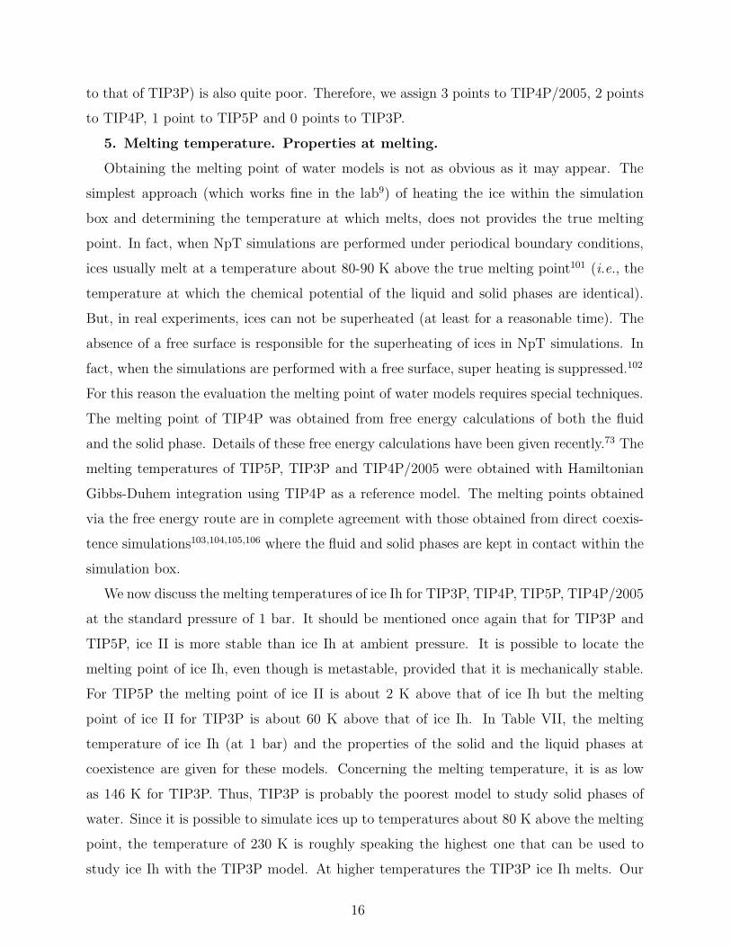
5. Melting temperature. Properties at melting.

Obtaining the melting point of water models is not as obvious as it may appear. The

simplest approach (which works fine in the lab9) of heating the ice within the simulation

box and determining the temperature at which melts, does not provides the true melting

point. In fact, when NpT simulations are performed under periodical boundary conditions,

ices usually melt at a temperature about 80-90 K above the true melting point101 (i.e., the

temperature at which the chemical potential of the liquid and solid phases are identical).

But, in real experiments, ices can not be superheated (at least for a reasonable time). The

absence of a free surface is responsible for the superheating of ices in NpT simulations. In

fact, when the simulations are performed with a free surface, super heating is suppressed.102

For this reason the evaluation the melting point of water models requires special techniques.

The melting point of TIP4P was obtained from free energy calculations of both the fluid

and the solid phase. Details of these free energy calculations have been given recently.73 The

melting temperatures of TIP5P, TIP3P and TIP4P/2005 were obtained with Hamiltonian

Gibbs-Duhem integration using TIP4P as a reference model. The melting points obtained

via the free energy route are in complete agreement with those obtained from direct coexis-

tence simulations103,104,105,106 where the fluid and solid phases are kept in contact within the

simulation box.

We now discuss the melting temperatures of ice Ih for TIP3P, TIP4P, TIP5P, TIP4P/2005

at the standard pressure of 1 bar. It should be mentioned once again that for TIP3P and

TIP5P, ice II is more stable than ice Ih at ambient pressure. It is possible to locate the

melting point of ice Ih, even though is metastable, provided that it is mechanically stable.

For TIP5P the melting point of ice II is about 2 K above that of ice Ih but the melting

point of ice II for TIP3P is about 60 K above that of ice Ih. In Table VII, the melting

temperature of ice Ih (at 1 bar) and the properties of the solid and the liquid phases at

coexistence are given for these models. Concerning the melting temperature, it is as low

as 146 K for TIP3P. Thus, TIP3P is probably the poorest model to study solid phases of

water. Since it is possible to simulate ices up to temperatures about 80 K above the melting

point, the temperature of 230 K is roughly speaking the highest one that can be used to

study ice Ih with the TIP3P model. At higher temperatures the TIP3P ice Ih melts. Our

16

estimates for the melting temperature of TIP4P, TIP4P/2005 and TIP5P are approximately

232 K, 252 K, and 274 K, respectively. The result for TIP4P is in good agreement with

the value reported by Gao et al.107 and Koyama et al108. Another interesting quantity

is the ratio of the normal melting temperature to the critical temperature, Tm/Tc. Since

the difference between the normal melting temperature and the triple point temperature

is of about 0.01 K, this ratio determines the range of existence of the liquid phase for the

considered model. Experimentally, Tm/Tc=0.42. The value of the ratio for TIP4P models

(TIP4P and TIP4P/2005) is essentially the same, 0.394, but it increases to 0.525 for TIP5P.

Thus TIP4P models describe significantly better the experimental range of existence of the

liquid phase for water. For TIP3P the ratio is considerably lower, 0.25, when the melting

temperature of ice Ih (146 K) is considered. But it increases to 0.36 using 210 K as the

melting temperature for the stable phase at normal melting for the TIP3P model which is

ice II.

Table VII also presents the coexistence properties (densities at coexistence, slope of the

melting curve dp/dT and enthalpy of melting). TIP4P/2005 provides the best estimates of

the coexistence densities and TIP5P gives a poor estimate of the density of ice Ih, and a

completely wrong prediction of the slope dp/dT . This is because, for TIP5P, the densities

of ice Ih and of the liquid are quite similar. On the other hand, no model is able to

reproduce the melting enthalpy. It is too small (three times lower) for TIP3P. The TIP4P

and TIP4P/2005 models do also underestimate the melting enthalpy but the errors are

much smaller, about 30% and 20%, respectively. Finally, TIP5P overestimates the melting

enthalpy by approximately a 20%.

Let us now try to provide a rational basis for the previous results. For three charge

models (TIP3P, TIP4P and TIP4P/2005) there is a clear correlation between the melting

temperature of ice Ih and the quadrupole moment of the molecule.54,56 Our conclusion is that

models locating the negative charge on the oxygen atom have low melting point temperatures

for ice Ih. Locating the negative charge shifted from the oxygen along the H-O-H bisector

increases the melting temperature. The improvement is better if the polarization correction

is used in the calculation of the vaporization enthalpy as a target property. When this is

done (as in TIP4P/2005) the melting point is about 20 K below the experimental value.

This is the closest you can get for the melting point of ice Ih with a three charge model

while still describing the vaporization enthalpy with the polarization correction of Berendsen

17

et al.51. The only way of reproducing the experimental melting point of ice Ih within three

charge models is to sacrify the vaporization enthalpy as a target property. In fact, we have

developed a model (denoted as TIP4P/Ice)35 which reproduces the melting point of ice Ih

but overestimates the vaporization enthalpy. The behaviour of TIP5P is different, it yields

a good prediction for the melting temperature in spite of having a low quadrupole moment.

Probably the fact that there are two negative charges instead of just one is the responsible

of this different behaviour. It is likely that locating the negative charge on the lone pair

electrons enhances the formation of hydrogen bonds in the solid phases provoking an increase

in the melting point.

TIP5P reproduces the melting temperature of water. But this is not for free, since

the estimate of the coexistence density of ice and of the dp/dT slope becomes then quite

poor. Conversely, TIP4P/2005 predicts a rather low melting temperature but it gives quite

reasonable estimates for the properties at melting. For this reason, there is no clear winner

in this test so we have decided to assign 2.5 points to both TIP5P and TIP4P/2005, 1 point

to TIP4P and 0 points to TIP3P.

6. Temperature of maximum density. Thermal coefficients α and κT .

The density of liquid water for the room pressure isobar as a function of the temperature

for TIP3P, SPC and TIP4P with a simple truncation of the Coulombic forces have been

reported by Jorgensen and Jenson.109. Recently, we have also calculated the liquid densities

at normal pressure36,50 for TIP3P, TIP4P, TIP5P and TIP4P/2005 using Ewald sums to

deal with long range Coulombic forces. Good agreement between our results and those

reported by Paschek was found.31 Our results are shown in Figure 6. All models do exhibit

a maximum in the density of water along the isobar. For some time it was believed that

TIP3P did not exhibit this maximum but it is now clear that the maximum also exists

for this model (although located at very low temperatures). In Table VIII, the location of

the TMD and the values of the thermal expansion coefficient (α ) and of the isothermal

compressibility (κT ) at room temperature and pressure are presented. It is clear that the

poorest description of the TMD is provided by TIP3P. The behaviour of TIP4P is noticeably

better. TIP4P/2005 reproduces nicely the density of water (and its maximum) for all the

temperatures along the room pressure isobar. We have shown recently50 that, —for three

charge models as TIP3P, TIP4P and TIP4P/2005— the difference between the TMD and

the melting temperature of ice is around 25 K (the experimental difference is 4 K). For

18

this reason, the location of the TMD correlates very well with the melting temperature.

TIP5P also reproduces the temperature at which the maximum density in water occurs.

For the TIP5P the difference between the melting point of ice Ih and the temperature of

the maximum in density is about 11 K. In Fig.6 the densities of TIP5P as obtained from

simulations using Ewald summation are presented. Notice that TIP5P does not reproduce

the experimental densities when Ewald summation is used. In the original paper where the

TIP5P model was proposed by Mahoney and Jorgensen the potential was truncated at 9 A.

In these conditions TIP5P reproduces the density of water at the maximum. It has been

noticed by other authors that in general, lower densities are obtained when Ewald sums are

implemented than when the electrostatic potential is merely truncated at a given distance.

The decrease in density is particularly noticeable in the case of the TIP5P model. For this

reason the maximum in density of the TIP5P model occurs at 285 K when Ewald sums are

used50,64 whereas the maximum takes place at 277 K when the potential is truncated at 9 A.

Fig.6 shows that for the TIP5P model when the whole normal pressure isobar is considered

(not just the maxima), the curvature is not correct. In other words, the dependence of the

density with temperature at constant pressure (given by the thermal expansion coefficient α)

is not properly predicted by TIP5P (see Table VIII). Importantly, this is also true when the

potential is truncated at 9 A. Therefore, TIP5P does not reproduces correctly α, neither with

the potential truncated at 9 A nor with Ewald sums. In summary, both TIP4P/2005 and

TIP5P reproduces the temperature at which the density maximum occurs. This is by design

since the TMD was used as a target property in both models. However, the description of the

complete room pressure isobar is much better in the TIP4P/2005 which reproduces nicely

the whole curve providing a very good estimate of the coefficient α. Also the estimate of κT

is better for TIP4P/2005. The excellent description of the densities along the isobar has an

interesting consequence. Since the vapour pressure of water is quite small up to relatively

high temperatures, orthobaric densities are essentially identical to those obtained from the

room pressure isobar. Therefore, a model describing correctly the equation of state along the

room pressure isobar will also provide reliable estimates of the orthobaric densities(at least,

at temperatures not too close to the critical one). Thus the good description of the ambient

pressure isobar of TIP4P/2005 explains in part the good description of the coexistence curve

presented previously. Although TIP5P estimates correctly the location of the TMD (when

using a cutoff for the electrostatic interactions), it does not yield satisfactory densities for

19

the the rest of the the room pressure isobar and this explains the poor performance in

describing orthobaric coexistence densities. Thus, using the TMD as a target property is a

good idea, but it is far better to use the complete room pressure isobar (of course including

the maximum) as a target property. For future developments of water potentials we do

really recommend to use the complete room pressure isobar as a target property. According

to the discussion above, we give 3 points to TIP4P/2005, 2 points to TIP5P, 1 point to

TIP4P and 0 points to TIP3P.

7. Structure of liquid water and ice.

The experimental oxygen-oxygen radial distribution function for liquid water and for ice

Ih will be compared to the predictions from the simulations. In Figure 7 the comparison is

made for liquid water. Experimental results are taken from Soper.110 TIP5P provides the

best estimate of the radial distribution function. The predictions of TIP4P/2005 are good

but the first peak is too high. TIP4P gives quite acceptable predictions but not as good

as the previous models. Once again, the discrepancy between the results for TIP3P and

experiment are notorious. In figure 8 the comparison is made for ice Ih at 77 K and 1 bar.

Experimental results are taken from Narten et al.111 The predictions of TIP4P/2005 are now

the best (although it overestimates again the height of the first peak). The results for TIP4P

are also very good. Both TIP5P and TIP3P fail in the description of the structure of the

solid beyond the first coordination shell. TIP4P/2005 provides good estimates of the radial

distribution functions but it overestimates the height of the first peak. It is likely than

quantum effects (which could be determined by using path integral simulations) may be

significant to understand the amplitude of the first maximum. Indeed, this has been shown

to be the case not only for liquid water112,113 but also for ice Ih as reported by Kusalik and

de la Pena114,115. Further work on this point is probably needed. There is no clear winner

concerning structural predictions (TIP5P performs better for water and TIP4P/2005 for ice

Ih). For this reason we have decided to give 2.5 points to both TIP5P and TIP4P/2005,

one point to TIP4P and zero points to TIP3P.

8. Equation of state of liquid water at high pressures.

In a number of geological applications the equation of state (EOS) of water at high

temperatures and pressures is needed. Therefore it is of interest to analyse the capacity of

these models to predict the behaviour of liquid water at high pressure. Figure 9 displays the

EOS for TIP3P, TIP4P, TIP4P/2005 and TIP5P along the 373 K isotherm for pressures up

20

to 24000bar (obtained with 360 water molecules). Experimental results are taken from the

EOS of Wagner116 and from the experimental measurements of Brown et al.117. TIP4P/2005

provides an excellent description of the EOS. The differences with experimental data increase

for TIP3P followed by TIP4P. The performance of TIP5P is quite poor. We thus assign 3

points to TIP4P/2005, 2 points to TIP3P, 1 point to TIP4P and 0 points to TIP5P.

9. Self-diffusion coefficient. We have computed the self-diffusion coefficient as a

function of temperature (at 1 bar) for TIP3P, TIP5P, TIP4P and TIP4P/2005. Simulations

were performed with the GROMACS47 package and the diffusion coefficients were determined

from the slope of the mean square displacement versus time (using 360 molecules). A

relaxation time of 5 ps was used for the thermostat and for the barostat. Results are

presented in Table IX. The diffusion coefficient of TIP3P is too high at all the temperatures

investigated. This suggests that the hydrogen bonding for this model is probably too weak.

Likely, the weakness of the hydrogen bond is also responsible of the low ice Ih melting

temperature and the loss of structure for the liquid phase beyond the first coordination

shell. This may be a big concern in simulation studies of proteins where there must be

a competition between intramolecular and intermolecular hydrogen bonds. The diffusion

coefficients of TIP4P are closer to experiment but they are still too high reflecting the fact

that using the vaporization enthalpy as a target property leads to highly diffusive water

models. TIP5P yields results in agreement with experimental data in the vicinity of 300

K but the departures from experiment greatly increase as the temperature moves away

from the ambient one. In fact, at 318 K the result furnished by TIP5P is almost the same

as that for TIP4P. Figure 10 shows that the slope of the line log D vs 1/T is quite poor

(TIP4P and even TIP3P are superior in this aspect). This seems to reflect the overall

results of TIP5P: good results at ambient conditions but becoming increasingly bad as one

moves away from that point. The best predictions are those of TIP4P/2005. Although a

little bit below the experimental values they show the correct trend in its dependence with

temperature. Within three charge models, the use of the polarization correction to describe

the vaporization enthalpy leads to water models with improved diffusion properties. That

was already true for SPC/E (which provides much better diffusion coefficients than SPC)

and seems also to be true for TIP4P/2005 (which provides much better estimates of the

diffusion coefficients than TIP4P). We give then 3 points to both TIP4P/2005, 2 points to

TIP5P, 1 point to TIP4P and zero points to TIP3P.

21

10. Dielectric constant.

Let us finish by presenting results for the dielectric constant of liquid water at room tem-

perature and pressure. Again, simulations were performed with the package GROMACS47

at room temperature and pressure. The simulations lasted 8 ns, and the system consisted of

360 molecules. The value of the dielectric constant is presented in Table X. TIP5P provides

the best estimate of the dielectric constant followed by TIP3P. TIP4P yields the worse value

for the dielectric constant. TIP4P/2005 predicts a better dielectric constant than TIP4P but

it is still far from the experimental value. It is obvious that the TIP4P charge distribution

tends to give low dielectric constants. This is the only property for which the TIP4P charge

distribution is in trouble against charge distributions with the negative charge located at

the oxygen atom. In fact, the dielectric constants of SPC and SPC/E are better than those

of TIP4P and TIP4P/2005, respectively, indicating that locating the charge on the oxygen

tends to give better predictions for the dielectric constant. Recently, Rick65 has studied in

detail the behaviour of the dielectric constant as a function of the dipole and quadrupole

moments for different water models. He has shown that a larger dipole increases the value

of the dielectric constant whereas a larger quadrupole decreases it. He proposed an equation

to correlate the dielectric constant of water models with these multipole moments:

ǫ = −85 + 98µ − 35.7QT (6)

where the dipole moment is given in Debye and QT in (Debye A). The dipole moments

of all water models are quite similar. However they differ significantly in the value of the

quadrupole moment. Thus, the lower value of the dielectric constant for TIP4P models is

a direct consequence of the higher quadrupole moment of these type of models. The higher

quadrupole moment of TIP4P/2005 was quite good to improve predictions for melting point

and phase diagram. Unfortunately, it also seems responsible for the low dielectric constant

of the model.

The dielectric constant is given by the fluctuations of the dipole moment of the sample. It

is thus related to the instantaneous values of the polarization of the sample. Non-polarizable

models attempt to incorporate (in a mean field way) the effect of the polarizability. Thus,

the dipole moments of non-polarizable models are higher than those of the gas phase. It

is likely that a property as the dielectric constant, depending so dramatically on just the

dipole moment fluctuations, can be hardly reproduced by an effective potential in which

22

the molecular charge cannot fluctuate. In fact, polarizable models tend to have higher

dielectric constants41 than their non-polarizable counterparts. If this is the case, the good

agreement of TIP3P and TIP5P may be somewhat forced. Probably, polarizable versions of

TIP3P and TIP5P will tend to give too high dielectric constants whereas the introduction of

polarizability will improve the predictions of models based on the TIP4P charge distribution.

Further work is required to analyse this issue in more detail since it is difficult at this stage

to establish definitive conclusions. Concerning the dielectric constant predictions, we give 3

points to TIP5P, 2 points to TIP3P, 1 point to TIP4P/2005 and 0 points to TIP4P.

VI. CONCLUSIONS

Table XI summarizes the scores obtained by the models for each of the test properties.

The final result is that TIP4P/2005 has obtained 27 points, TIP5P 14, TIP4P 13 and TIP3P

6 over a maximum possible number of 30 points. For most of the properties TIP4P/2005

yielded the best performance. The main exception is the dielectric constant for which

TIP4P/2005 yields a too low value. For the second position, TIP5P and TIP4P obtained

very similar scores. TIP5P improves the melting point predictions, TMD, dielectric constant

and diffusivity with respect to TIP4P, but it is clearly worse in phase diagram predictions,

critical point, density of ices, and high pressure behaviour. In that respect TIP5P and

TIP4P yielded a similar performance and the choice for the one or the other potential may

depend on the considered property to study. The less satisfactory model, well below any

of the others is TIP3P (see Table XI). Somewhat surprisingly TIP3P is probably the most

used model in simulations of biomolecules. In our opinion the only reason to continue using

TIP3P is that certain force fields were optimized to be used with TIP3P water. It is not fully

obvious whether the force fields must be used with a given water model. Some researchers

have challenged this idea.118 In any case, it is clear that new force fields should also be built

around better water models.

We have not included in the comparison SPC or SPC/E models. The performance of SPC

is certainly better than that of TIP3P. This is due to the fact, that if the negative charge is

located on the oxygen, the larger OH bond length of SPC, and the tetrahedral bond angle

increases the values of the quadrupole moment and this improves the performance of the

model. However, SPC/E yields an overall better performance than SPC. In fact, it improves

23

the prediction of almost all of the properties. The performance of SPC/E, in case it would

have been included in the test, would have been better than that of TIP5P and TIP4P but

well below that of TIP4P/2005. The number of points obtained by SPC/E would have been

about 21 points (3 for vapour-liquid equilibria, 2 points for surface tension, 2 points for the

density of ices, 1 point for the phase diagram, 1 point for the melting properties, 1 point for

the TMD, α and κT , 2 points for structure predictions, 3 points for the equation of state at

high pressures, 3 points for the diffusion coefficient and 3 points for the dielectric constant).

Thus, overall SPC/E improves the predictions with respect to TIP4P and TIP5P but it is

well below the number of points obtained by TIP4P/2005.

Why the performance of TIP4P/2005 is in general so good? TIP4P/2005 is just a TIP4P

model with the hydrogen charge augmented from 0.52 e to 0.556 e and with the value

of ǫ/kB increased from 73 K to 93 K (the values of σ and dOM are quite similar in both

models). It has taken more than twenty years to realize that these two small changes improve

dramatically the performance of the model. The steps leading to TIP4P/2005 are basically

three. First, the realization of the fact that TIP4P provided a better phase diagram than

SPC/E. Secondly, the attempt to improve the prediction of the melting temperature could

not be done without accepting the idea of introducing a correction term in the calculation

of the vaporization enthalpy. The idea, first introduced by Berendsen51 et al., enabled them

to transform SPC into SPC/E which, in our opinion, is a much better model than SPC. The

same could also be useful within the TIP4P geometry, and the final result is TIP4P/2005.

But there was an additional refinement. Using the TMD as a target property (as first

done by TIP5P) or, even better, fitting the whole room pressure isobar could improve the

overall performance. Thus, TIP4P/2005 incorporated this property as a target property. In

summary, TIP4P/2005 takes from TIP4P the charge distribution (which yields a reasonable

prediction of the phase diagram of water), from SPC/E the use of Berendsen et al. correction

to the vaporization enthalpy, and from TIP5P the use of the TMD as a target property. The

resulting model, predicts quite nicely the orthobaric densities, critical temperature, surface

tension, densities of the different solid phases of water, phase diagram, melting properties

(with a reasonable prediction of the melting point about 20 K below the experimental value),

TMD, isothermal compressibility, coefficient of thermal expansion, structure of water and

ice. The properties analysed here cover a temperature range from 120 to 640 K and pressures

up to 30 000 bar.

24

Obviously TIP4P/2005 is not the last word in water potentials and have some deficiencies.

It fails in the prediction of the vapour properties (vapour pressure, dew densities, critical

pressure, second virial coefficient) and in the prediction of the dielectric constant in the

liquid phase. However, it really points out clearly the limits that can be achieved by rigid

non-polarizable models. We believe that inclusion of polarizability within a TIP4P/2005-like

model (with an adequate fitting of the parameters) would yield further improvement. The

extreme sensitivity of phase diagram to the water potential model may help in developing

new potential models for water. Now that it is possible to evaluate phase diagrams (both

vapour-liquid and fluid-solid) or the TMD on relatively routine basis, it sounds a good idea

to extend the incorporation of the phase diagram and the room pressure isobar as target

properties in the fitting (and/or checking) of new water models. Although there may be a

current of opinion suggesting that polarizable models have not yet improved the performance

of non-polarizable models, it is our belief that we have not worked hard enough to refine a

reliable polarizable model for water. For the time being, TIP4P/2005 can be considered as a

reliable and cheap model of water offering good performance over a wide range of conditions.

Since TIP4P/2005 is a minor modification of the model proposed by Bernal and Fowler46

in 1933, one may say that we have spend seventy five years in refining their parameters to

finally obtain a reliable model of water for the condensed phases.

Acknowledgments

It is a pleasure to acknowledge to L. G. MacDowell, E.G.Noya, C. McBride, and R. G.

Fernandez for many helpful discussions and for their contribution to different parts of this

work. Discussions with E.de Miguel (Huelva), A.Patrykiejew (Lublin), I.Nezbeda (Prague)

are also gratefully acknowledged. This work has been funded by grants FIS2007-66079-C02-

01 from the DGI (Spain), S-0505/ESP/0229 from the CAM, MTKD-CT-2004-509249 from

the European Union and 910570 from the UCM.

1 P. Ball, Life’s Matrix. A biography of Water (University of California Press, Berkeley, 2001).

2 J. P. Poirier, Nature 299, 683 (1982).

25

3 D. Eisenberg and W. Kauzmann, The Structure and Properties of Water (Oxford University

Press, London, 1969).

4 V. F. Petrenko and R. W. Whitworth, Physics of Ice (Oxford University Press, 1999).

5 J. L. Finney, Phil.Trans.R.Soc.Lond.B 359, 1145 (2004).

6 M. Chaplin, http://www.lsbu.ac.uk/water/ (2005).

7 J. L. Finney, J. Molec. Liq. 90, 303 (2001).

8 G. Tammann, Kristallisieren und Schmelzen (Johann Ambrosius Barth, Leipzig, 1903).

9 P. W. Bridgman, Proc. Am. Acad. Sci. Arts 47, 441 (1912).

10 C. Lobban, J. L. Finney, and W. F. Kuhs, Nature 391, 268 (1998).

11 C. G. Salzmann, P. G. Radaelli, A. Hallbrucker, E. Mayer, and J. L. Finney, Science 311, 1758

(2006).

12 C. G. Venkatesh, S. A. Rice, and A. H. Narten, Science 186, 927 (1974).

13 P. G. Debenedetti, J. Phys. Cond. Mat. 15, R1669 (2003).

14 O. Mishima, L. D. Calvert, and E. Whalley, Nature 310, 393 (1984).

15 P. H. Poole, F. Sciortino, U. Essmann, and H. E. Stanley, Nature 360, 324 (1992).

16 O. Mishima and H. E. Stanley, Nature 396, 329 (1998).

17 G. J. Kroes, Surface Science 275, 365 (1992).

18 M. T. Suter, P. U. Andersson, and J. B. C. Petterson, J. Chem. Phys. 125, 174704 (2006).

19 J. G. Dash, A. W. Rempel, and J. S. Wettlaufer, Reviews of Modern Physics 78, 695 (2006).

20 H. Bluhm, D. F. Ogletree, C. S. Fadley, Z. Hussain, and M. Salmeron, J.Phys.Conden.Matter

14, L227 (2002).

21 F. Paesani and G. A. Voth, J.Phys.Chem.C 112, 324 (2008).

22 P. Jedlovszky, L. Partay, P. N. M. Hoang, S. Picaud, P. von Hessberg, and J. N. Crowley, J.

Am. Chem. Soc. 128, 15300 (2006).

23 V. Buch, H. Groenzin, I. Li, M. J. Shultz, and E. Tosatti, Proc. Am. Acad. Sci. Arts 105, 5969

(2008).

24 D. Chandler, Nature 437, 640 (2005).

25 S. J. Wierzchowski and P. A. Monson, J. Phys. Chem. B 111, 7274 (2007).

26 J. A. Barker and R. O. Watts, Chem. Phys. Lett. 3, 144 (1969).

27 A. Rahman and F. H. Stillinger, J. Chem. Phys. 55, 3336 (1971).

28 R. M. Lynden-Bell, J. C. Rasaiah, and J. P. Noworyta, Pure Appl. Chem. 73, 1721 (2001).

26

29 K. M. Aberg, A. P. Lyubartsev, S. P. Jacobsson, and A. Laaksonen, J. Chem. Phys. 120, 3770

(2004).

30 M. Ferrario, G. Ciccotti, E. Spohr, T. Cartailler, and P.Turq, J. Chem. Phys. 117, 4947 (2002).

31 D. Paschek, J. Chem. Phys. 120, 6674 (2004).

32 C. R. W. Guimaraes, G. Barreiro, C. A. F. de Oliveria, and R. B. de Alencastro, Brazil. J.

Phys. 34, 126 (2004).

33 B. Guillot, J. Molec. Liq. 101, 219 (2002).

34 E. Sanz, C. Vega, J. L. F. Abascal, and L. G. MacDowell, Phys. Rev. Lett. 92, 255701 (2004).

35 J. L. F. Abascal, E. Sanz, R. G. Fernandez, and C. Vega, J. Chem. Phys. 122, 234511 (2005).

36 J. L. F. Abascal and C. Vega, J. Chem. Phys. 123, 234505 (2005).

37 M. D. Morse and S. A. Rice, J. Chem. Phys. 76, 650 (1982).

38 E. Whalley, J. Chem. Phys. 81, 4087 (1984).

39 P. A. Monson and D. A. Kofke, in Advances in Chemical Physics, edited by I. Prigogine and

S. A. Rice (John Wiley and Sons, 2000), vol. 115, p. 113.

40 P. A. Monson, AIChE J 54, 1122 (2008).

41 P. Paricaud, M. Predota, A. A. Chialvo, and P. T. Cummings, J. Chem. Phys. 122, 244511

(2005).

42 B. Chen, J. Xing, and J. I. Siepmann, J. Phys. Chem. B 104, 2378 (2000).

43 W. L. Jorgensen, J. Chandrasekhar, J. D. Madura, R. W. Impey, and M. L. Klein, J. Chem.

Phys. 79, 926 (1983).

44 M. W. Mahoney and W. L. Jorgensen, J. Chem. Phys. 112, 8910 (2000).

45 H. J. C. Berendsen, J. P. M. Postma, W. F. van Gunsteren, and J. Hermans, Intermolecular

Forces, ed. B. Pullman, page 331 (Reidel, Dordrecht, 1982).

46 J. D. Bernal and R. H. Fowler, J. Chem. Phys. 1, 515 (1933).

47 E. Lindahl, B. Hess, and D. van der Spoel, J. Molecular Modeling 7, 306 (2001).

48 F. H. Stillinger and A. Rahman, J. Chem. Phys. 60, 1545 (1974).

49 L. A. Baez and P. Clancy, J. Chem. Phys. 101, 9837 (1994).

50 C. Vega and J. L. F. Abascal, J. Chem. Phys. 123, 144504 (2005).

51 H. J. C. Berendsen, J. R. Grigera, and T. P. Straatsma, J. Phys. Chem. 91, 6269 (1987).

52 E. Sanz, C. Vega, J. L. F. Abascal, and L. G. MacDowell, J. Chem. Phys. 121, 1165 (2004).

53 C. Vega, E. Sanz, and J. L. F. Abascal, J. Chem. Phys. 122, 114507 (2005).

27

54 J. L. F. Abascal and C. Vega, Phys. Chem. Chem. Phys. 9, 2775 (2007).

55 J. L. F. Abascal and C. Vega, Phys. Rev. Lett. 98, 237801 (2007).

56 J. L. F. Abascal and C. Vega, J. Phys. Chem. C 111, 15811 (2007).

57 G. N. Patey and J. P. Valleau, J. Chem. Phys. 64, 170 (1976).

58 J. L. Finney, J. E. Quinn, and J. O. Baum, in Water Science Reviews 1, edited by F. Franks

(Cambridge University Press, Cambridge, 1985).

59 K. Watanabe and M. L. Klein, Chem. Phys. 131, 157 (1989).

60 G. A. Tribello and B. Slater, Chem. Phys. Lett. 425, 246 (2006).

61 K. M. Benjamin, A. J. Schultz, and D. A. Kofke, J.Phys.Chem.C 111, 16021 (2007).

62 K. M. Benjamin, J. K. Singh, A. J. Schultz, and D. A. Kofke, J.Phys.Chem.B 111, 11463

(2007).

63 D. van der Spoel, P. J. van Maaren, and H. J. C. Berendsen, J. Chem. Phys. 108, 10220 (1998).

64 M. Lısal, J. Kolafa, and I. Nezbeda, J. Chem. Phys. 117, 8892 (2002).

65 S. W. Rick, J. Chem. Phys. 120, 6085 (2004).

66 Y. Yonetani, J. Chem. Phys. 124, 204501 (2006).

67 M. P. Allen and D. J. Tildesley, Computer Simulation of Liquids (Oxford University Press,

1987).

68 D. Frenkel and B. Smit, Understanding Molecular Simulation (Academic Press, London, 2002).

69 B. Garzon, S. Lago, and C. Vega, Chem. Phys. Lett. 231, 366 (1994).

70 M. Parrinello and A. Rahman, J. Appl. Phys. 52, 7182 (1981).

71 S. Yashonath and C. N. R. Rao, Molec. Phys. 54, 245 (1985).

72 D. Frenkel and A. J. C. Ladd, J. Chem. Phys. 81, 3188 (1984).

73 C. Vega, E. Sanz, E. G. Noya, and J. L. F. Abascal, J. Phys. Condens. Matter 20, 153101

(2008).

74 J. K. Johnson, J. A. Zollweg, and K. E. Gubbins, Molec. Phys. 78, 591 (1993).

75 D. A. Kofke, J. Chem. Phys. 98, 4149 (1993).

76 D. A. Kofke, Phys. Rev. Lett. 74, 122 (1995).

77 M. Lisal, W. R. Smith, and I. Nezbeda, Fluid Phase Equilib. 181, 127 (2001).

78 M. Lisal, I. Nezbeda, and W. R. Smith, J. Phys. Chem. B 108, 7412 (2004).

79 C. Vega, J. L. F. Abascal, and I. Nezbeda, J. Chem. Phys. 125, 034503 (2006).

80 C. C. Liew, H. Inomata, and K. Arai, Fluid.Phase.Equilibria 144, 287 (1998).

28

81 J. R. Errington and A. Z. Panagiotopoulos, J. Phys. Chem. B 102, 7470 (1998).

82 C. Vega and E. de Miguel, J. Chem. Phys. 126, 154707 (2007).

83 J. S. Rowlinson and B. Widom, Molecular Theory of Capillarity (Clarendon Press, Oxford,

1982).

84 G. J. Gloor, G. Jackson, F. J. Blas, and E. de Miguel, J. Chem. Phys. 123, 134703 (2005).

85 F. Chen and P. E. Smith, J. Chem. Phys. 126, 221101 (2007).

86 G. W. Robinson, S. Singh, S. B. Zhu, and M. W. E. (editors), Water in biology, chemistry and

physics: Experimental Overviews and Computational Methodologies (Singapore:World Scien-

tific, 1996).

87 H. J. White, J. V. Sengers, D. B. Neumann, and J. C. Bellows, IAPWS Release on the Surface

Tension of Ordinary Water Substance (1995).

88 A. Ghoufi, F. Goujon, V. Lachet, and P. Malfreyt, J. Chem. Phys. 128, 154716 (2008).

89 J. Lopez-Lemus, G. A. Chapela, and J. Alejandre, J. Chem. Phys. 128, 174703 (2008).

90 A. Baranyai, A. Bartok, and A. A. Chialvo, J. Chem. Phys. 123, 54502 (2005).

91 C. Vega, C. McBride, E. Sanz, and J. L. Abascal, Phys. Chem. Chem. Phys. 7, 1450 (2005).

92 T. James, D. J. Wales, and J. Hernandez-Rojas, Chem. Phys. Lett. 415, 302 (2005).

93 L. Pauling, J. Am. Chem. Soc. 57, 2680 (1935).

94 L. G. MacDowell, E. Sanz, C. Vega, and L. F. Abascal, J. Chem. Phys. 121, 10145 (2004).

95 V. Buch, P. Sandler, and J. Sadlej, J. Phys. Chem. B 102, 8641 (1998).

96 J. L. Aragones, E. G. Noya, J. L. F. Abascal, and C. Vega, J. Chem. Phys. 127, 154518 (2007).

97 E. G. Noya, C. Menduina, J. L. Aragones, and C. Vega, J. Phys. Chem. C 111, 15877 (2007).

98 A. D. Fortes, I. G. Wood, M. Alfredsson, L. Vocadlo, and K. S. Knight, J. Appl. Cryst. 38,

612 (2005).

99 B. Kamb, Acta Cryst. 17, 1437 (1964).

100 C. Vega, J. L. F. Abascal, E. Sanz, L. G. MacDowell, and C. McBride, J. Phys. Cond. Mat.

17, S3283 (2005).

101 C. McBride, C. Vega, E. Sanz, L. G. MacDowell, and J. L. F. Abascal, Molec. Phys. 103, 1

(2005).

102 C. Vega, M. Martin-Conde, and A. Patrykiejew, Molec. Phys. 104, 3583 (2006).

103 O. A. Karim and A. D. J. Haymet, J. Chem. Phys. 89, 6889 (1988).

104 R. G. Fernandez, J. L. F. Abascal, and C. Vega, J. Chem. Phys. 124, 144506 (2006).

29

105 J. Wang, S. Yoo, J. Bai, J. R. Morris, and X. C. Zeng, J. Chem. Phys. 123, 036101 (2005).

106 D. Quigley and P. M. Rodger, J. Chem. Phys. 128, 154518 (2008).

107 G. T. Gao, X. C. Zeng, and H. Tanaka, J. Chem. Phys. 112, 8534 (2000).

108 Y. Koyama, H. Tanaka, G. Gao, and X.C.Zeng, J. Chem. Phys. 121, 7926 (2004).

109 W. L. Jorgensen and C. Jenson, J. Comput. Chem. 19, 1179 (1998).

110 A. K. Soper, Chem. Phys. 258, 121 (2000).

111 A. H. Narten, C. G. Venkatesh, and S. A. Rice, J. Chem. Phys. 64, 1106 (1976).

112 H. A. Stern and B. J. Berne, J. Chem. Phys. 115, 7622 (2001).

113 L. Hernandez de la Pena and P. G. Kusalik, J. Chem. Phys. 121, 5992 (2004).

114 L. Hernandez de la Pena and P. G. Kusalik, J. Am. Chem. Soc. 127, 5246 (2005).

115 L. Hernandez de la Pena, M. S. Gulam Razul, and P. G. Kusalik, J. Chem. Phys. 123, 144506

(2005).

116 W. Wagner, A. Saul, and A. Pruss, J. Phys. Chem. Ref. Data 23, 515 (1994).

117 E. H. Abramson and J. M. Brown, Geochimica et Cosmochimica Acta 68, 1827 (2004).

118 D. R. Nutt and J. C. Smith, J. Chem. Theory and Comput. 3, 1550 (2007).

119 R. J. Hemley, A. P. Jephcoat, H. K. Mao, C. S. Zha, L. W. Finger, and D. E. Cox, Nature

330, 737 (1987).

120 W. L. Jorgensen and J. Tirado-Rives, Proc. Am. Acad. Sci. Arts 102, 6665 (2005).

121 A. D. Fortes, I. G. Wood, J. P. Brodholt, and L. Vocadlo, J. Chem. Phys. 119, 4567 (2003).

122 B. Kamb, W. C. Hamilton, S. J. LaPlaca, and A. Prakash, J. Chem. Phys. 55, 1934 (1971).

30

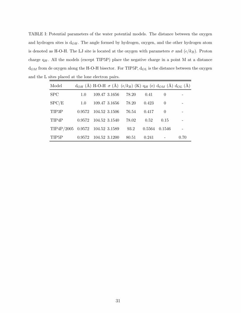
TABLE I: Potential parameters of the water potential models. The distance between the oxygen

and hydrogen sites is dOH . The angle formed by hydrogen, oxygen, and the other hydrogen atom

is denoted as H-O-H. The LJ site is located at the oxygen with parameters σ and (ǫ/kB). Proton

charge qH . All the models (except TIP5P) place the negative charge in a point M at a distance

dOM from de oxygen along the H-O-H bisector. For TIP5P, dOL is the distance between the oxygen

and the L sites placed at the lone electron pairs.

Model dOH (A) H-O-H σ (A) (ǫ/kB) (K) qH (e) dOM (A) dOL (A)

SPC 1.0 109.47 3.1656 78.20 0.41 0 -

SPC/E 1.0 109.47 3.1656 78.20 0.423 0 -

TIP3P 0.9572 104.52 3.1506 76.54 0.417 0 -

TIP4P 0.9572 104.52 3.1540 78.02 0.52 0.15 -

TIP4P/2005 0.9572 104.52 3.1589 93.2 0.5564 0.1546 -

TIP5P 0.9572 104.52 3.1200 80.51 0.241 - 0.70

31

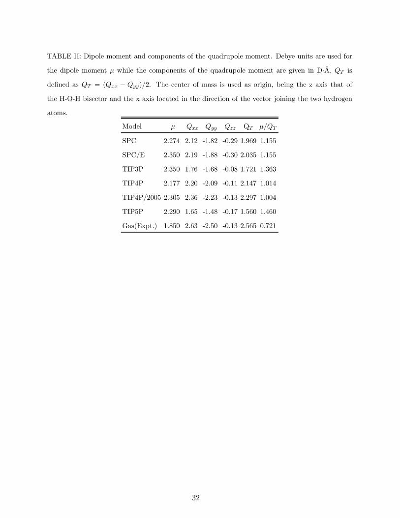
TABLE II: Dipole moment and components of the quadrupole moment. Debye units are used for

the dipole moment µ while the components of the quadrupole moment are given in D·A. QT is

defined as QT = (Qxx − Qyy)/2. The center of mass is used as origin, being the z axis that of

the H-O-H bisector and the x axis located in the direction of the vector joining the two hydrogen

atoms.

Model µ Qxx Qyy Qzz QT µ/QT

SPC 2.274 2.12 -1.82 -0.29 1.969 1.155

SPC/E 2.350 2.19 -1.88 -0.30 2.035 1.155

TIP3P 2.350 1.76 -1.68 -0.08 1.721 1.363

TIP4P 2.177 2.20 -2.09 -0.11 2.147 1.014

TIP4P/2005 2.305 2.36 -2.23 -0.13 2.297 1.004

TIP5P 2.290 1.65 -1.48 -0.17 1.560 1.460

Gas(Expt.) 1.850 2.63 -2.50 -0.13 2.565 0.721

32

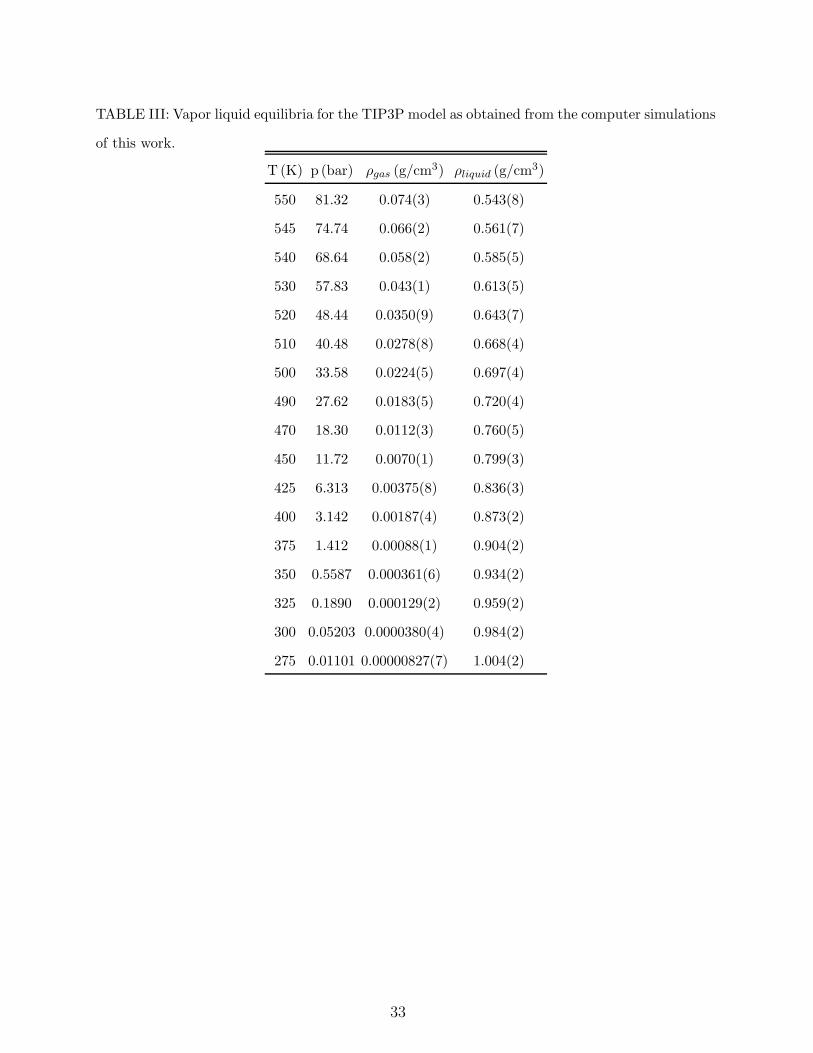
TABLE III: Vapor liquid equilibria for the TIP3P model as obtained from the computer simulations

of this work.

T (K) p (bar) ρgas (g/cm3) ρliquid (g/cm3)

550 81.32 0.074(3) 0.543(8)

545 74.74 0.066(2) 0.561(7)

540 68.64 0.058(2) 0.585(5)

530 57.83 0.043(1) 0.613(5)

520 48.44 0.0350(9) 0.643(7)

510 40.48 0.0278(8) 0.668(4)

500 33.58 0.0224(5) 0.697(4)

490 27.62 0.0183(5) 0.720(4)

470 18.30 0.0112(3) 0.760(5)

450 11.72 0.0070(1) 0.799(3)

425 6.313 0.00375(8) 0.836(3)

400 3.142 0.00187(4) 0.873(2)

375 1.412 0.00088(1) 0.904(2)

350 0.5587 0.000361(6) 0.934(2)

325 0.1890 0.000129(2) 0.959(2)

300 0.05203 0.0000380(4) 0.984(2)

275 0.01101 0.00000827(7) 1.004(2)

33

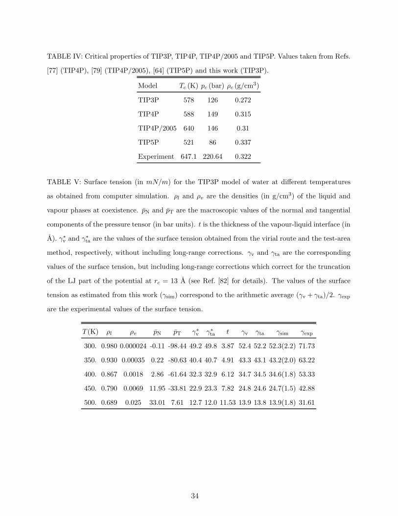
TABLE IV: Critical properties of TIP3P, TIP4P, TIP4P/2005 and TIP5P. Values taken from Refs.

[77] (TIP4P), [79] (TIP4P/2005), [64] (TIP5P) and this work (TIP3P).

Model Tc (K) pc (bar) ρc (g/cm3)

TIP3P 578 126 0.272

TIP4P 588 149 0.315

TIP4P/2005 640 146 0.31

TIP5P 521 86 0.337

Experiment 647.1 220.64 0.322

TABLE V: Surface tension (in mN/m) for the TIP3P model of water at different temperatures

as obtained from computer simulation. ρl and ρv are the densities (in g/cm3) of the liquid and

vapour phases at coexistence. pN and pT are the macroscopic values of the normal and tangential

components of the pressure tensor (in bar units). t is the thickness of the vapour-liquid interface (in

A). γ∗

v and γ∗

ta are the values of the surface tension obtained from the virial route and the test-area

method, respectively, without including long-range corrections. γv and γta are the corresponding

values of the surface tension, but including long-range corrections which correct for the truncation

of the LJ part of the potential at rc = 13 A (see Ref. [82] for details). The values of the surface

tension as estimated from this work (γsim) correspond to the arithmetic average (γv + γta)/2. γexp

are the experimental values of the surface tension.

T (K) ρl ρv pN pT γ∗

v γ∗

ta t γv γta γsim γexp

300. 0.980 0.000024 -0.11 -98.44 49.2 49.8 3.87 52.4 52.2 52.3(2.2) 71.73

350. 0.930 0.00035 0.22 -80.63 40.4 40.7 4.91 43.3 43.1 43.2(2.0) 63.22

400. 0.867 0.0018 2.86 -61.64 32.3 32.9 6.12 34.7 34.5 34.6(1.8) 53.33

450. 0.790 0.0069 11.95 -33.81 22.9 23.3 7.82 24.8 24.6 24.7(1.5) 42.88

500. 0.689 0.025 33.01 7.61 12.7 12.0 11.53 13.9 13.8 13.9(1.8) 31.61

34

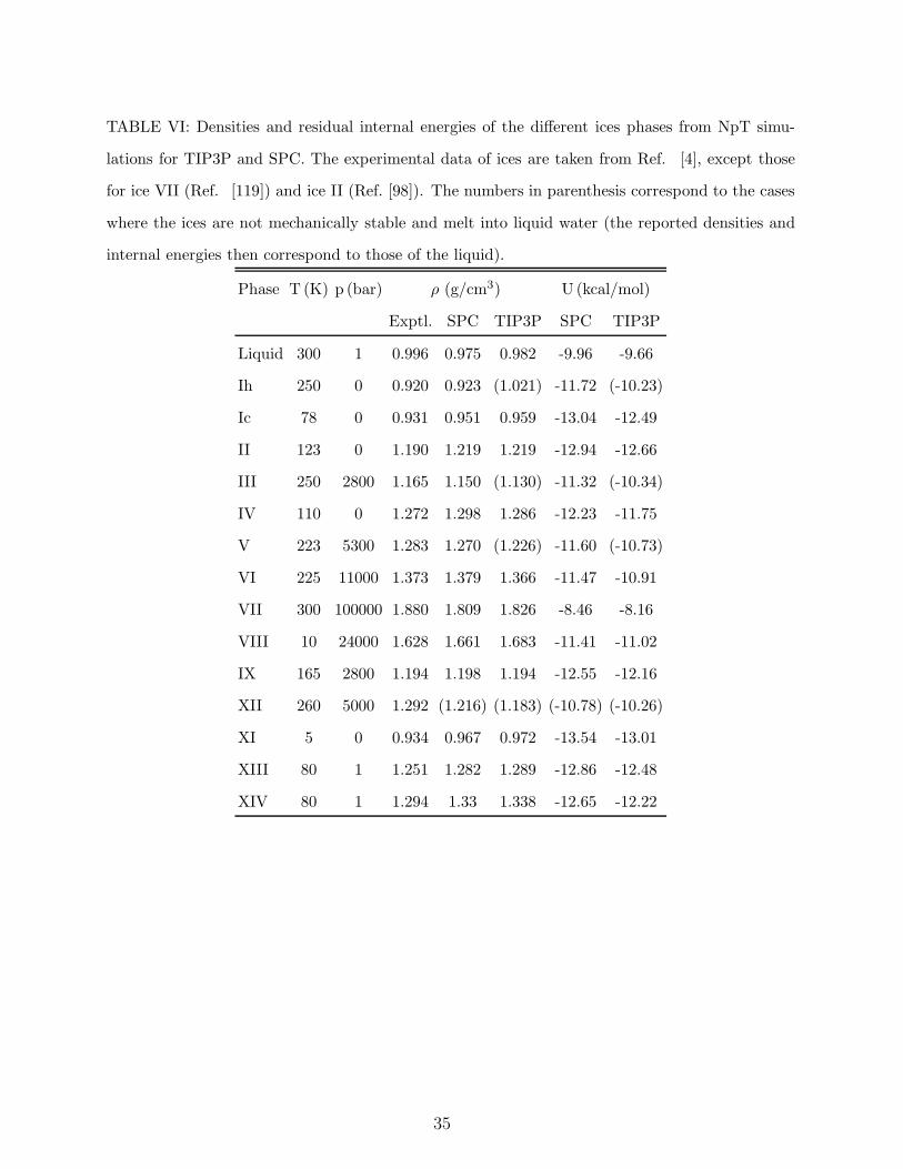
TABLE VI: Densities and residual internal energies of the different ices phases from NpT simu-

lations for TIP3P and SPC. The experimental data of ices are taken from Ref. [4], except those

for ice VII (Ref. [119]) and ice II (Ref. [98]). The numbers in parenthesis correspond to the cases

where the ices are not mechanically stable and melt into liquid water (the reported densities and

internal energies then correspond to those of the liquid).

Phase T (K) p (bar) ρ (g/cm3) U (kcal/mol)

Exptl. SPC TIP3P SPC TIP3P

Liquid 300 1 0.996 0.975 0.982 -9.96 -9.66

Ih 250 0 0.920 0.923 (1.021) -11.72 (-10.23)

Ic 78 0 0.931 0.951 0.959 -13.04 -12.49

II 123 0 1.190 1.219 1.219 -12.94 -12.66

III 250 2800 1.165 1.150 (1.130) -11.32 (-10.34)

IV 110 0 1.272 1.298 1.286 -12.23 -11.75

V 223 5300 1.283 1.270 (1.226) -11.60 (-10.73)

VI 225 11000 1.373 1.379 1.366 -11.47 -10.91

VII 300 100000 1.880 1.809 1.826 -8.46 -8.16

VIII 10 24000 1.628 1.661 1.683 -11.41 -11.02

IX 165 2800 1.194 1.198 1.194 -12.55 -12.16

XII 260 5000 1.292 (1.216) (1.183) (-10.78) (-10.26)

XI 5 0 0.934 0.967 0.972 -13.54 -13.01

XIII 80 1 1.251 1.282 1.289 -12.86 -12.48

XIV 80 1 1.294 1.33 1.338 -12.65 -12.22

35

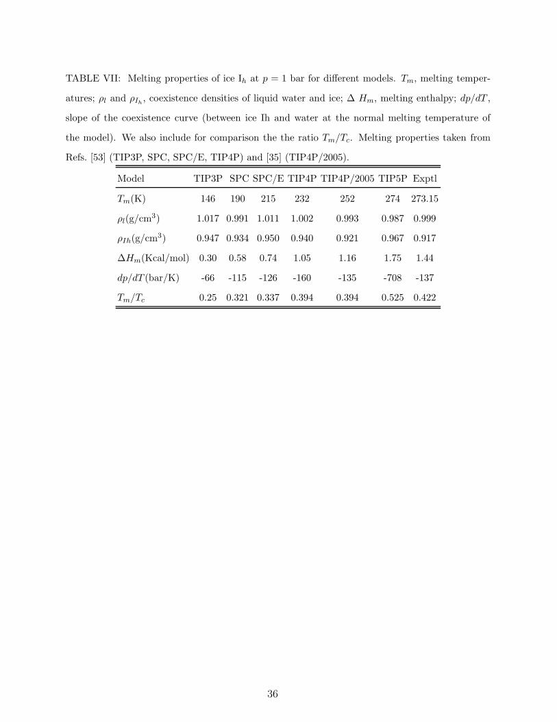
TABLE VII: Melting properties of ice Ih at p = 1 bar for different models. Tm, melting temper-

atures; ρl and ρIh, coexistence densities of liquid water and ice; ∆ Hm, melting enthalpy; dp/dT ,

slope of the coexistence curve (between ice Ih and water at the normal melting temperature of

the model). We also include for comparison the the ratio Tm/Tc. Melting properties taken from

Refs. [53] (TIP3P, SPC, SPC/E, TIP4P) and [35] (TIP4P/2005).

Model TIP3P SPC SPC/E TIP4P TIP4P/2005 TIP5P Exptl

Tm(K) 146 190 215 232 252 274 273.15

ρl(g/cm3) 1.017 0.991 1.011 1.002 0.993 0.987 0.999

ρIh(g/cm3) 0.947 0.934 0.950 0.940 0.921 0.967 0.917

∆Hm(Kcal/mol) 0.30 0.58 0.74 1.05 1.16 1.75 1.44

dp/dT (bar/K) -66 -115 -126 -160 -135 -708 -137

Tm/Tc 0.25 0.321 0.337 0.394 0.394 0.525 0.422

36

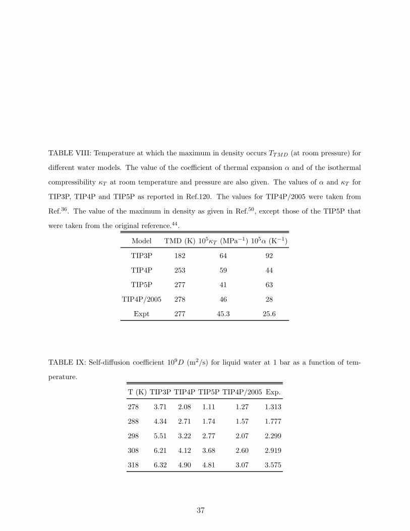
TABLE VIII: Temperature at which the maximum in density occurs TTMD (at room pressure) for

different water models. The value of the coefficient of thermal expansion α and of the isothermal

compressibility κT at room temperature and pressure are also given. The values of α and κT for

TIP3P, TIP4P and TIP5P as reported in Ref.120. The values for TIP4P/2005 were taken from

Ref.36. The value of the maximum in density as given in Ref.50, except those of the TIP5P that

were taken from the original reference.44.

Model TMD (K) 105κT (MPa−1) 105α (K−1)

TIP3P 182 64 92

TIP4P 253 59 44

TIP5P 277 41 63

TIP4P/2005 278 46 28

Expt 277 45.3 25.6

TABLE IX: Self-diffusion coefficient 109D (m2/s) for liquid water at 1 bar as a function of tem-

perature.

T (K) TIP3P TIP4P TIP5P TIP4P/2005 Exp.

278 3.71 2.08 1.11 1.27 1.313

288 4.34 2.71 1.74 1.57 1.777

298 5.51 3.22 2.77 2.07 2.299

308 6.21 4.12 3.68 2.60 2.919

318 6.32 4.90 4.81 3.07 3.575

37

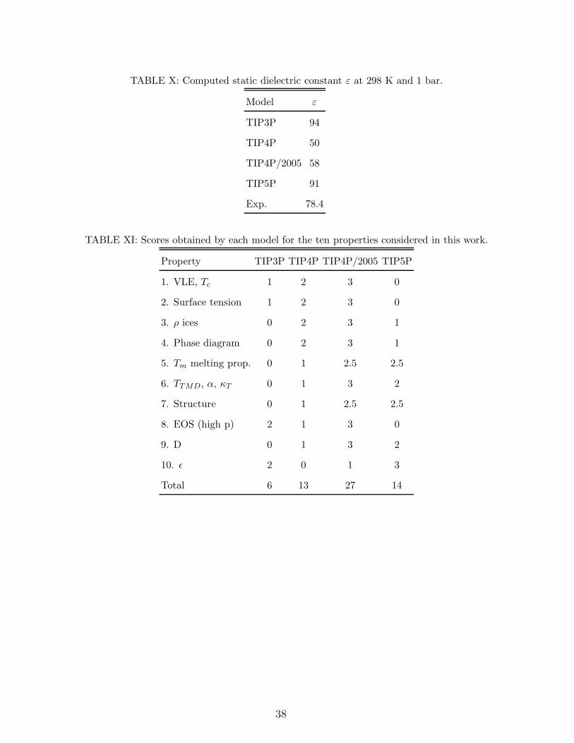
TABLE X: Computed static dielectric constant ε at 298 K and 1 bar.

Model ε

TIP3P 94

TIP4P 50

TIP4P/2005 58

TIP5P 91

Exp. 78.4

TABLE XI: Scores obtained by each model for the ten properties considered in this work.

Property TIP3P TIP4P TIP4P/2005 TIP5P

1. VLE, Tc 1 2 3 0

2. Surface tension 1 2 3 0

3. ρ ices 0 2 3 1

4. Phase diagram 0 2 3 1

5. Tm melting prop. 0 1 2.5 2.5

6. TTMD, α, κT 0 1 3 2

7. Structure 0 1 2.5 2.5

8. EOS (high p) 2 1 3 0

9. D 0 1 3 2

10. ǫ 2 0 1 3

Total 6 13 27 14

38

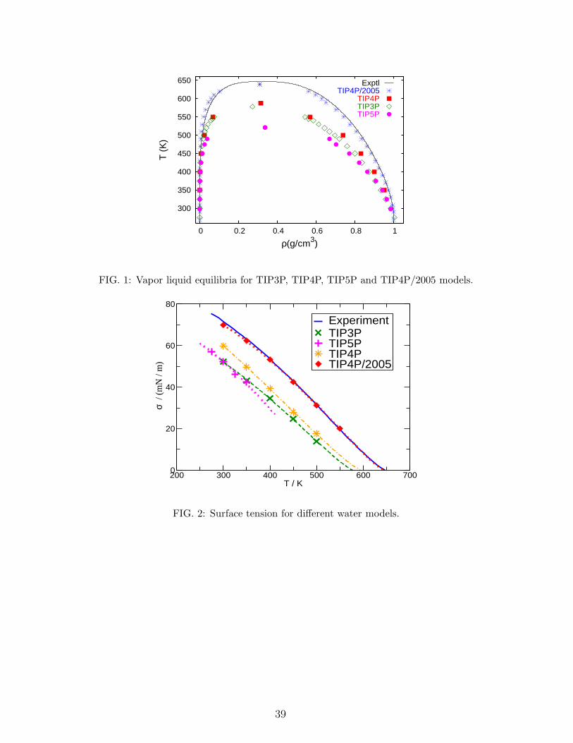
300

350

400

450

500

550

600

650

0 0.2 0.4 0.6 0.8 1

T (

K)

ρ(g/cm3)

ExptlTIP4P/2005

TIP4PTIP3PTIP5P

FIG. 1: Vapor liquid equilibria for TIP3P, TIP4P, TIP5P and TIP4P/2005 models.

200 300 400 500 600 700T / K

0

20

40

60

80

σ /

(mN

/ m

)

Experiment TIP3PTIP5PTIP4PTIP4P/2005

FIG. 2: Surface tension for different water models.

39

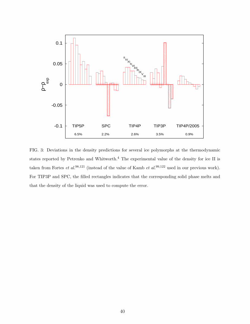
-0.1

-0.05

0

0.05

0.1ρ−

ρ

TIP5P SPC TIP4P TIP3P TIP4P/2005

exp

6.5% 2.2% 2.6% 3.5% 0.9%

IIIV

XIIc

VIXII

IhIX

VIII

FIG. 3: Deviations in the density predictions for several ice polymorphs at the thermodynamic

states reported by Petrenko and Whitworth.4 The experimental value of the density for ice II is

taken from Fortes et al.98,121 (instead of the value of Kamb et al.99,122 used in our previous work).

For TIP3P and SPC, the filled rectangles indicates that the corresponding solid phase melts and

that the density of the liquid was used to compute the error.

40

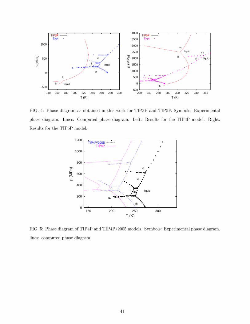
-500

0

500

1000

140 160 180 200 220 240 260 280 300

p (

MP

a)

T (K)

liquid

Ih

II

V

liquidIh

II

TIP3PExpt

-500

0

500

1000

1500

2000

2500

3000

3500

4000

220 240 260 280 300 320 340 360

p (

MP

a)

T (K)

liquid

Ih

II

VI

liquidVI

VII

TIP5PExpt

FIG. 4: Phase diagram as obtained in this work for TIP3P and TIP5P. Symbols: Experimental

phase diagram. Lines: Computed phase diagram. Left. Results for the TIP3P model. Right.

Results for the TIP5P model.

0

200

400

600

800

1000

1200

150 200 250 300

p (M

Pa)

T (K)

liquid

Ih

IIIII

V

VI

TIP4P/2005TIP4P

FIG. 5: Phase diagram of TIP4P and TIP4P/2005 models. Symbols: Experimental phase diagram,

lines: computed phase diagram.

41

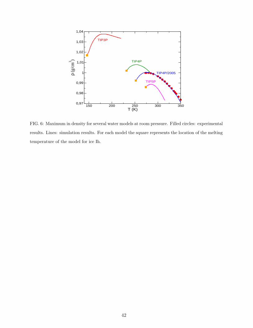
150 200 250 300 350T (K)

0,97

0,98

0,99

1

1,01

1,02

1,03

1,04

ρ (g

/cm

3 )

TIP3P

TIP4P/2005

TIP5P

TIP4P

FIG. 6: Maximum in density for several water models at room pressure. Filled circles: experimental

results. Lines: simulation results. For each model the square represents the location of the melting

temperature of the model for ice Ih.

42

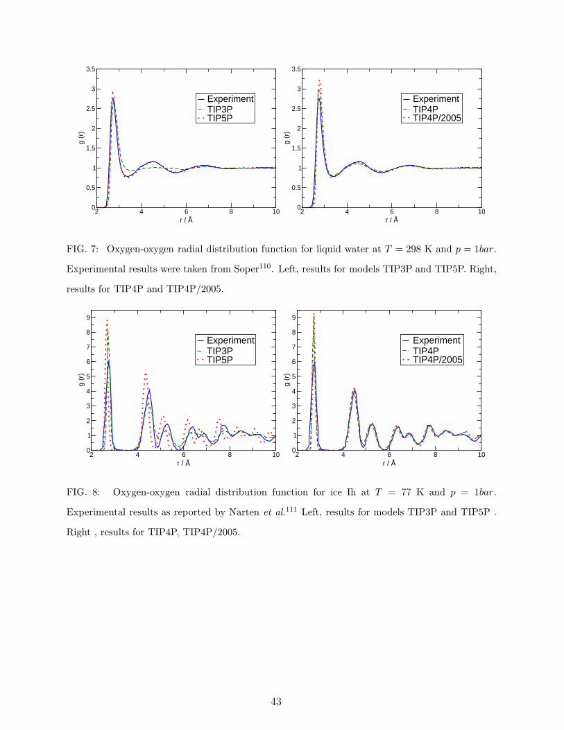
2 4 6 8 10r / Å

0

0.5

1

1.5

2

2.5

3

3.5

g (r

)

Experiment TIP3PTIP5P

2 4 6 8 10r / Å

0

0.5

1

1.5

2

2.5

3

3.5

g (r

)

Experiment TIP4PTIP4P/2005

FIG. 7: Oxygen-oxygen radial distribution function for liquid water at T = 298 K and p = 1bar.

Experimental results were taken from Soper110. Left, results for models TIP3P and TIP5P. Right,

results for TIP4P and TIP4P/2005.

2 4 6 8 10r / Å

0

1

2

3

4

5

6

7

8

9

g (r

)

Experiment TIP3PTIP5P

2 4 6 8 10r / Å

0

1

2

3

4

5

6

7

8

9

g (r

)

Experiment TIP4PTIP4P/2005

FIG. 8: Oxygen-oxygen radial distribution function for ice Ih at T = 77 K and p = 1bar.

Experimental results as reported by Narten et al.111 Left, results for models TIP3P and TIP5P .

Right , results for TIP4P, TIP4P/2005.

43

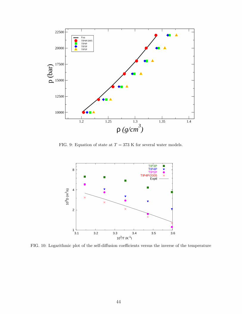
1.2 1.25 1.3 1.35 1.4

ρ (g/cm3)

10000

12500

15000

17500

20000

22500

p (b

ar)

Exp.

TIP4P/2005TIP4PTIP3PTIP5P

FIG. 9: Equation of state at T = 373 K for several water models.

1

2

4

8

3.1 3.2 3.3 3.4 3.5 3.6

109 D

(m

2 /s)

103/T (K-1)

TIP3PTIP4PTIP5P

TIP4P/2005Exptl

FIG. 10: Logarithmic plot of the self-diffusion coefficients versus the inverse of the temperature

44