Essays in Applied Econometrics and Education

CitationBarrios, Thomas. 2014. Essays in Applied Econometrics and Education. Doctoral dissertation, Harvard University.

Permanent linkhttp://nrs.harvard.edu/urn-3:HUL.InstRepos:12274546

Terms of UseThis article was downloaded from Harvard University’s DASH repository, and is made available under the terms and conditions applicable to Other Posted Material, as set forth at http://nrs.harvard.edu/urn-3:HUL.InstRepos:dash.current.terms-of-use#LAA

Share Your StoryThe Harvard community has made this article openly available.Please share how this access benefits you. Submit a story .

Accessibility

Essays in Applied Econometrics and Education

A dissertation presented

by

Thomas Barrios

to

The Department of Economics

in partial fulfillment of the requirements

for the degree of

Doctor of Philosophy

in the subject of

Economics

Harvard University

Cambridge, Massachusetts

April 2014

c© 2014 Thomas Barrios

All rights reserved.

Dissertation Advisors:Professor Edward GlaeserProfessor Lawrence Katz

Author:Thomas Barrios

Essays in Applied Econometrics and Education

Abstract

This dissertation consists of three essays. First, we explore the implications of correlations that do

not vanishing for units in different clusters for the actual and estimated precision of least squares

estimators. Our main theoretical result is that with equal-sized clusters, if the covariate of interest is

randomly assigned at the cluster level, only accounting for nonzero covariances at the cluster level,

and ignoring correlations between clusters as well as differences in within-cluster correlations, leads

to valid confidence intervals. Next, we examine the choice of pairs in matched pair randomized

experiments. We show that stratifying on the conditional expectation of the outcome given baseline

variables is optimal in matched-pair randomized experiments. Last, we measure the effect of decreased

course availability on grades, degree attainment, and transfer to four-year colleges using a regression

discontinuity from course enrollment queues due to oversubscribed courses. We find that in the short

run students substitute unavailable courses with others.

iii

Contents

Abstract . . . . . . . . . . . . . . . . . . . . . . . . . . . . . . . . . . . . . . . . . . . . iiiAcknowledgments . . . . . . . . . . . . . . . . . . . . . . . . . . . . . . . . . . . . . . . ix

Introduction 1

1 Clustering, Spatial Correlations and Randomization Inference 31.1 Introduction . . . . . . . . . . . . . . . . . . . . . . . . . . . . . . . . . . . . . . . 31.2 Framework . . . . . . . . . . . . . . . . . . . . . . . . . . . . . . . . . . . . . . . 51.3 Spatial Correlation Patterns in Earnings . . . . . . . . . . . . . . . . . . . . . . . . 81.4 Randomization Inference . . . . . . . . . . . . . . . . . . . . . . . . . . . . . . . . 171.5 Randomization Inference with Cluster-level Randomization . . . . . . . . . . . . . . 191.6 Variance Estimation Under Misspecification . . . . . . . . . . . . . . . . . . . . . . 211.7 Spatial Correlation in State Averages . . . . . . . . . . . . . . . . . . . . . . . . . . 231.8 A Small Simulation Study . . . . . . . . . . . . . . . . . . . . . . . . . . . . . . . 261.9 Conclusion . . . . . . . . . . . . . . . . . . . . . . . . . . . . . . . . . . . . . . . 29

2 Optimal Stratification in Randomized Experiments 302.1 Introduction . . . . . . . . . . . . . . . . . . . . . . . . . . . . . . . . . . . . . . . 302.2 Main Result . . . . . . . . . . . . . . . . . . . . . . . . . . . . . . . . . . . . . . . 34

2.2.1 General solution to the matching problem . . . . . . . . . . . . . . . . . . . 412.3 Matching in Practice . . . . . . . . . . . . . . . . . . . . . . . . . . . . . . . . . . 432.4 Inference in Matched Pair Randomization . . . . . . . . . . . . . . . . . . . . . . . 45

2.4.1 Treatment Compliance . . . . . . . . . . . . . . . . . . . . . . . . . . . . . 462.5 Model Selection and Prediction Methods . . . . . . . . . . . . . . . . . . . . . . . . 46

2.5.1 AIC and BIC . . . . . . . . . . . . . . . . . . . . . . . . . . . . . . . . . . 472.5.2 Ridge and Lasso . . . . . . . . . . . . . . . . . . . . . . . . . . . . . . . . 50

2.6 Data and Simulations . . . . . . . . . . . . . . . . . . . . . . . . . . . . . . . . . . 512.6.1 Dataset descriptions . . . . . . . . . . . . . . . . . . . . . . . . . . . . . . 512.6.2 Data generating process . . . . . . . . . . . . . . . . . . . . . . . . . . . . 532.6.3 Benchmark performance . . . . . . . . . . . . . . . . . . . . . . . . . . . . 56

iv

2.6.4 Choice of matching variable . . . . . . . . . . . . . . . . . . . . . . . . . . 572.6.5 Are standard errors the correct size? . . . . . . . . . . . . . . . . . . . . . . 572.6.6 Performance with smaller training set . . . . . . . . . . . . . . . . . . . . . 592.6.7 Performance in small experiments . . . . . . . . . . . . . . . . . . . . . . . 592.6.8 Performance in large experiments . . . . . . . . . . . . . . . . . . . . . . . 60

2.7 Literature . . . . . . . . . . . . . . . . . . . . . . . . . . . . . . . . . . . . . . . . 612.7.1 Extensions to other randomization settings . . . . . . . . . . . . . . . . . . 66

2.8 Conclusion . . . . . . . . . . . . . . . . . . . . . . . . . . . . . . . . . . . . . . . 68

3 Course Availability and College Enrollment: Evidence from administrative data andenrollment discontinuities 693.1 Introduction . . . . . . . . . . . . . . . . . . . . . . . . . . . . . . . . . . . . . . . 693.2 Institutional Background and Data . . . . . . . . . . . . . . . . . . . . . . . . . . . 72

3.2.1 Course Enrollment . . . . . . . . . . . . . . . . . . . . . . . . . . . . . . . 733.2.2 Instrument Construction . . . . . . . . . . . . . . . . . . . . . . . . . . . . 74

3.3 Identification and Reduced-Form Evidence . . . . . . . . . . . . . . . . . . . . . . 773.3.1 Identification . . . . . . . . . . . . . . . . . . . . . . . . . . . . . . . . . . 773.3.2 First Stage . . . . . . . . . . . . . . . . . . . . . . . . . . . . . . . . . . . 803.3.3 Validity Checks . . . . . . . . . . . . . . . . . . . . . . . . . . . . . . . . . 823.3.4 No Sorting Across Wait List Position . . . . . . . . . . . . . . . . . . . . . 833.3.5 Reduced Form Evidence . . . . . . . . . . . . . . . . . . . . . . . . . . . . 85

3.4 IV Results . . . . . . . . . . . . . . . . . . . . . . . . . . . . . . . . . . . . . . . . 873.4.1 Course Enrollment . . . . . . . . . . . . . . . . . . . . . . . . . . . . . . . 883.4.2 GPA and Persistence . . . . . . . . . . . . . . . . . . . . . . . . . . . . . . 913.4.3 Enrollment at 4-year and other 2-year colleges . . . . . . . . . . . . . . . . 91

3.5 Subgroup Analysis and Robustness Checks . . . . . . . . . . . . . . . . . . . . . . 923.6 Conclusions . . . . . . . . . . . . . . . . . . . . . . . . . . . . . . . . . . . . . . . 95

References 96

Appendix A Appendix to Chapter 1 104A.1 Supplementary Results . . . . . . . . . . . . . . . . . . . . . . . . . . . . . . . . . 104

Appendix B Appendix to Chapter 2 111B.1 Supplementary Results . . . . . . . . . . . . . . . . . . . . . . . . . . . . . . . . . 111B.2 Supplementary Tables . . . . . . . . . . . . . . . . . . . . . . . . . . . . . . . . . . 121

Appendix C Appendix to Chapter 3 125C.1 Supplementary Tables . . . . . . . . . . . . . . . . . . . . . . . . . . . . . . . . . . 125

v

List of Tables

1.1 Sample Sizes . . . . . . . . . . . . . . . . . . . . . . . . . . . . . . . . . . . . . . 81.2 Summary Statistics . . . . . . . . . . . . . . . . . . . . . . . . . . . . . . . . . . . 91.3 Estimates for Clustering Variances for Demeaned Log Earnings . . . . . . . . . . . 131.4 p-values for Mantel Statistics, based on 10,000,000 draws and one-sided alternatives 251.5 Size of t-tests (in %) using different variance estimators (500,000 draws). . . . . . . 28

2.1 Counter example where treatment effect not independent of (X, ε) . . . . . . . . . . 412.2 Dataset Summary Statistics . . . . . . . . . . . . . . . . . . . . . . . . . . . . . . 552.3 DGP Descriptions 1-3 . . . . . . . . . . . . . . . . . . . . . . . . . . . . . . . . . 562.4 DGP Descriptions 4-6 . . . . . . . . . . . . . . . . . . . . . . . . . . . . . . . . . 572.5 Mean Squared Error for Multiple Randomization Methods . . . . . . . . . . . . . . 582.6 Size control for Multiple Randomization Methods . . . . . . . . . . . . . . . . . . 582.7 Power for Multiple Randomization Methods . . . . . . . . . . . . . . . . . . . . . 59

3.1 Hypothetical Enrollment Log . . . . . . . . . . . . . . . . . . . . . . . . . . . . . . 753.2 Summary Statistics: Race . . . . . . . . . . . . . . . . . . . . . . . . . . . . . . . . 763.3 Summary Statistics: Demographics . . . . . . . . . . . . . . . . . . . . . . . . . . . 773.4 First Stage OLS Regressions . . . . . . . . . . . . . . . . . . . . . . . . . . . . . . 823.5 TSLS Estimates of Effects on Course Enrollment . . . . . . . . . . . . . . . . . . . 893.6 TSLS Estimates of Effects on Course Enrollment (CCT) . . . . . . . . . . . . . . . 903.7 TSLS Estimates of Effects on GPA and Persistence (CCT) . . . . . . . . . . . . . . 913.8 TSLS Estimates of Effects on Four-Year College and Two-Year College Enrollment

(CCT) . . . . . . . . . . . . . . . . . . . . . . . . . . . . . . . . . . . . . . . . . . 92

B.1 Mean Squared Error for Multiple Randomization Methods 1 . . . . . . . . . . . . . 121B.2 Size control for Multiple Randomization Methods 1 . . . . . . . . . . . . . . . . . . 121B.3 Power for Multiple Randomization Methods 1 . . . . . . . . . . . . . . . . . . . . . 122B.4 Mean Squared Error for Multiple Randomization Methods 2 . . . . . . . . . . . . . 122B.5 Size control for Multiple Randomization Methods 2 . . . . . . . . . . . . . . . . . . 122B.6 Power for Multiple Randomization Methods 2 . . . . . . . . . . . . . . . . . . . . 123B.7 Mean Squared Error for Multiple Randomization Methods 3 . . . . . . . . . . . . . 123

vi

B.8 Size control for Multiple Randomization Methods 3 . . . . . . . . . . . . . . . . . . 123B.9 Power for Multiple Randomization Methods 3 . . . . . . . . . . . . . . . . . . . . 124

C.1 Cubic Local Polynomial Results, (CCT) . . . . . . . . . . . . . . . . . . . . . . . . 126C.2 Local Linear TSLS, with control variables (BW of 5) . . . . . . . . . . . . . . . . . 127C.3 Local Linear TSLS, with more extensive control variables (BW of 5) . . . . . . . . 128C.4 Local Linear TSLS, with more extensive control variables (BW of 3) . . . . . . . . 129

vii

List of Figures

1.1 Covariance of Demeaned Log(Earnings) by Distance Between Individuals . . . . . . 111.2 Covariance of Demeaned Log(Earnings) by Distance Between Individuals . . . . . . 121.3 States with minimum wage higher than federal minimum wage . . . . . . . . . . . . 151.4 New England/East North Central States . . . . . . . . . . . . . . . . . . . . . . . . 16

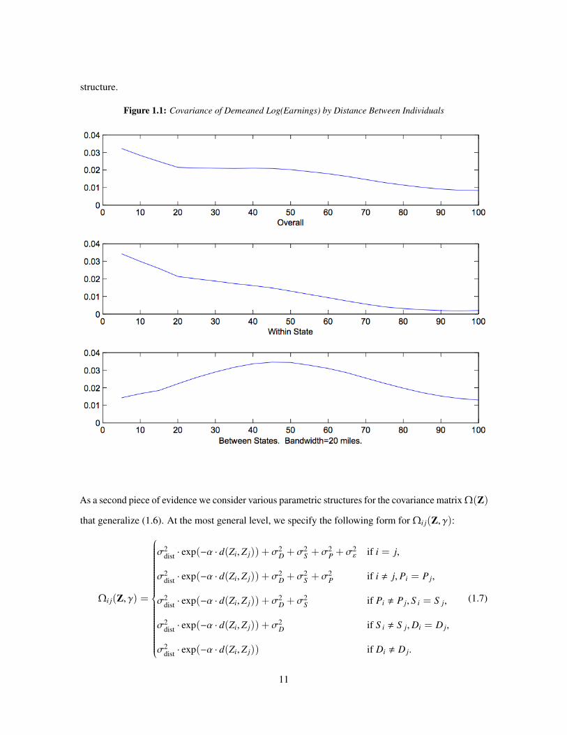
2.1 Counter example where treatment effect not independent of (X, ε) . . . . . . . . . . 422.2 How auxiliary data is used in Matched Pair Randomization . . . . . . . . . . . . . . 44

3.1 First Stage: Mean Enrollment in Wait-listed Section as a Function of Relative WaitList Position . . . . . . . . . . . . . . . . . . . . . . . . . . . . . . . . . . . . . . . 81

3.2 Smoothness on Covariates: Race and Citizenship Indicators . . . . . . . . . . . . . . 833.3 Smoothness on Covariates: Age, Gender, a priori Education . . . . . . . . . . . . . . 843.4 No Sorting Across Wait-list position . . . . . . . . . . . . . . . . . . . . . . . . . . 853.5 Enrollment in Other Sections, all subjects, concurrent term . . . . . . . . . . . . . . 863.6 Enrollment in Other Sections in the same subject, concurrent term . . . . . . . . . . 873.7 Stayed in School, 1 year . . . . . . . . . . . . . . . . . . . . . . . . . . . . . . . . 88

viii

Acknowledgments

Financial support for research in the first chapter was generously provided through NSF grant 0820361.

My coauthors and I are grateful for comments by participants in the econometrics lunch seminar at

Harvard University, and in particular for discussions with Gary Chamberlain. I am grateful to my Ph.D.

advisers Gary Chamberlain, Ed Glaeser, Guido Imbens, and Larry Katz for their generous guidance

in writing the second chapter. I thank Don Rubin, Max Kasy, Claudia Goldin, Stefano DellaVigna,

Roland Fryer, Michael Kremer, Sendhil Mullainathan, Jose Montiel Olea, Raj Chetty, Rick Hornbeck,

Nathaniel Hilger, and Silvia Robles for helpful comments. I am grateful to seminar participants at the

Harvard Labor, Development, and Econometrics workshops and at the MIT Development workshop.

Financial support for research in the second chapter was generously provided through an Education

Innovation Lab Research Fellowship. My coauthors and I thank Larry Katz and Ed Glaeser for helpful

comments on the third chapter. We thank Dean Jerry Rosenberg for helpful information on registration

and wait lists.

ix

To my parents, Susan Ipongi, Greg Butler, Gail Bunch, Michele Thompson, RichardRankins, Robert Lawson, Moori Schiesel-Manning, Richard Nolan, David Lee, andTheresa Olele.

x

Introduction

This dissertation consists of three chapters. The first examines clustering, spatial correlation and

randomization inference. The second explores optimal stratification in matched pair randomized

experiments. The third uses evidence from administrative data and enrollment discontinuities to

examine the effect course availability on college enrollment.

The first chapter is motivated by the observation that it is standard practice in empirical work to allow

for clustering in the error covariance matrix if the explanatory variables of interest vary at a more

aggregate level than the units of observation. Often, however, the structure of the error covariance

matrix is more complex, with correlations varying in magnitude within clusters, and not vanishing

between clusters. Here we explore the implications of such correlations for the actual and estimated

precision of least squares estimators. We show that with equal sized clusters, if the covariate of interest

is randomly assigned at the cluster level, only accounting for non-zero covariances at the cluster level,

and ignoring correlations between clusters, leads to valid standard errors and confidence intervals.

However, in many cases this may not suffice. For example, state policies exhibit substantial spatial

correlations. As a result, ignoring spatial correlations in outcomes beyond that accounted for by the

clustering at the state level, may well bias standard errors. We illustrate our findings using the 5%

public use census data. Based on these results we recommend researchers assess the extent of spatial

correlations in explanatory variables beyond state level clustering, and if such correlations are present,

take into account spatial correlations beyond the clustering correlations typically accounted for.

The second chapter is motivated by the question of how best to randomize with many baseline

1

covariates. We show that stratifying on the conditional expectation of the outcome given baseline

variables is optimal in matched-pair randomized experiments. The assignment minimizes the variance

of the post-treatment difference in mean outcomes between treatment and controls. Optimal pairing

depends only on predicted values of outcomes for experimental units, where the predicted values

are the conditional expectations. After randomization, both frequentist inference and randomization

inference depend only on the actual strata chosen and not on estimated predicted values. This gives

experimenters a way to use big data (possibly more covariates than the number of experimental units)

ex-ante while maintaining simple post-experiment inference techniques. Optimizing the randomization

with respect to one outcome allows researchers to credibly signal the outcome of interest prior to the

experiment. Inference can be conducted in the standard way by regressing the outcome on treatment

and strata indicators. We illustrate the application of the methodology by running simulations based

on a set of field experiments. We find that optimal designs have mean squared errors 23% less than

randomized designs, on average. In one case, mean squared error is 43% less than randomized

designs.

The third chapter examines the effect course availability on college enrollment. Community colleges

serve close to half of the undergraduate students in the United States and tuition at two-year public/non-

profit colleges is mostly a public expenditure. We measure the effect of decreased course availability

on grades, degree attainment, and transfer to four-year colleges using a regression discontinuity from

course enrollment queues due to oversubscribed courses. Using a panel from a large California

community college and the National Student Clearinghouse we find that in the short run students

substitute unavailable courses with others. We find no significant effects on later outcomes, given the

precision of our tests, however we cannot rule out economically significant effects.

2

Chapter 1

Clustering, Spatial Correlations and

Randomization Inference1

1.1 Introduction

Many economic studies that analyze the effects of interventions on economic behavior study inter-

ventions that are constant within clusters whereas the outcomes vary at a more disaggregate level. In

a typical example, and the one we focus on in this paper, outcomes are measured at the individual

level, whereas interventions or treatments vary only at the state (cluster) level. Often, the effect of

interventions is estimated using least squares regression. Since the mid-eighties (Liang and Zeger,

1986; Moulton, 1986), empirical researchers in social sciences have generally been aware of the

implications of within-cluster correlations in outcomes for the precision of such estimates. The typical

approach is to allow for correlation between outcomes in the same cluster in the specification of the

error covariance matrix. However, there may well be more complex correlation patterns in the data.

1Co-authored with Rebecca Diamond, Guido W. Imbens, and Michal Kolesar

3

Correlation in outcomes between individuals may extend beyond state boundaries, it may vary in

magnitude between states, and it may be stronger in more narrowly defined geographical areas.

In this paper we investigate the implications, for the repeated sampling variation of least squares

estimators based on individual-level data, of the presence of correlation structures beyond those which

are constant within and identical across states, and which vanish between states. First, we address the

empirical question whether in census data on earnings with states as clusters such correlation patterns

are present to a substantially meaningful degree. We estimate general spatial correlations for the

logarithm of earnings, and find that, indeed, such correlations are present, with substantial correlations

within groups of nearby states, and correlations within smaller geographic units (specifically pumas,

public use microdata areas) considerably larger than within states. Second, we address whether

accounting for such correlations is important for the properties of confidence intervals for the effects of

state-level regulations. We report theoretical results, as well as demonstrate their relevance both using

illustrations based on earnings data and state regulations, and Monte Carlo evidence. The theoretical

results show that if covariate values are as good as randomly assigned to clusters, implying there is

no spatial correlation in the covariates beyond the clusters, variance estimators that incorporate only

cluster-level outcome correlations remain valid despite the misspecification of the error-covariance

matrix. Whether this theoretical result is useful in practice depends on the magnitude of the spatial

correlations in the covariates. We provide some illustrations that show that, given the spatial correlation

patterns we find in the individual-level variables, spatial correlations in state level regulations can have

a substantial impact on the precision of estimates of the effects of interventions.

The paper draws on three strands of literature that have largely evolved separately. First, it is related

to the literature on clustering and difference-in-differences estimation, where a primary focus is on

adjustments to standard errors to take into account clustering of explanatory variables. See, e.g., Liang

and Zeger (1986), Moulton (1986), Bertrand, Duflo, and Mullainathan (2004), Hansen (2009), and

the textbook discussions in Angrist and Pischke (2009), Diggle, Heagerty, Liang, and Zeger (2002),

and Wooldridge (2002). Second, the current paper draws on the literature on spatial statistics. Here a

major focus is on the specification and estimation of the covariance structure of spatially linked data.

4

For a textbook discussion see Schabenberger and Gotway (2004). In interesting recent work Bester,

Conley and Hansen (2009) and Ibragimov and Müller (2009) link some of the inferential issues in the

spatial and clustering literatures. Finally, we use results from the literature on randomization inference

going back to Fisher (1925) and Neyman (1923). For a recent discussion see Rosenbaum (2002).

Although the calculation of Fisher exact p-values based on randomization inference is frequently

used in the spatial statistics literature (e.g., Schabenberger and Gotway, 2004), and sometimes in the

clustering literature (Bertrand, Duflo and Mullainathan, 2004; Abadie, Diamond, and Hainmueller,

2009), Neyman’s approach to constructing confidence intervals using the randomization distribution is

rarely used in these settings. We will argue that the randomization perspective provides useful insights

into the interpretation of confidence intervals in the context of spatially linked data.

The paper is organized as follows. In Section 1.2 we introduce the basic set-up. Next, in Section 1.3,

using census data on earnings, we establish the presence of spatial correlation patterns beyond the

constant-within-state correlations typically allowed for. In Section 1.4 we discuss randomization-based

methods for inference, first focusing on the case with randomization at the individual level. Section

1.5 extends the results to cluster-level randomization. In Section 1.6, we present the main theoretical

results. We show that if cluster-level covariates are randomly assigned to the clusters, the standard

variance estimator based on within-cluster correlations can be robust to misspecification of the error-

covariance matrix. Next, in Section 1.7 we show, using Mantel-type tests, that a number of regulations

exhibit substantial regional correlations, suggesting that ignoring the error correlation structure may

not be justified. Section 1.8 reports the results of a small simulation study. Section 1.9 concludes.

Proofs are collected in an appendix.

1.2 Framework

Consider a setting where we have information on N units, say individuals in the United States, indexed

by i = 1, . . . , N. Associated with each unit is a location Zi, measuring latitude and longitude for

individual i. Associated with a location z are a unique puma P(z) (public use microdata area, a

5

census-defined area with at least 100,000 individuals), a state S (z), and a division D(z) (also a census

defined concept, with nine divisions in the United States). In our application the sample is divided

into 9 divisions, which are then divided into a total of 49 states (we leave out individuals from Hawaii

and Alaska, and include the District of Columbia as a separate state), which are then divided into

2,057 pumas. For individual i, with location Zi, let Pi, S i, and Di, denote the puma, state, and division

associated with the location Zi. The distance d(z, z′) between two locations z and z′ is defined as

the shortest distance, in miles, on the earth’s surface connecting the two points. To be precise, let

z = (zlat, zlong) be the latitude and longitude of a location. Then the formula for the distance in miles

between two locations z and z′ we use is

d(z, z′) = 3, 959 × arccos(cos(zlong − z′long) · cos(zlat) · cos(z′lat) + sin(zlat) · sin(z′lat)).

In this paper, we focus primarily on estimating the slope coefficient β in a linear regression of some

outcome Yi (e.g., the logarithm of individual level earnings for working men) on a binary intervention

Wi (e.g., a state-level regulation), of the form

Yi = α+ β ·Wi + εi. (1.1)

A key issue is that the explanatory variable Wi may be constant withing clusters of individuals. In our

application Wi varies at the state level.

Let ε denote the N-vector with typical element εi, and let Y, W, P, S, and D, denote the N-vectors

with typical elements Yi, Wi, Pi, S i, and Di. Let ιN denote the N-vector of ones, let Xi = (1, Wi), and

let X and Z denote the N × 2 matrices with ith rows equal to Xi and Zi, respectively, so that we can

write in matrix notation

Y = ιN · α+ W · β+ ε = X(α β

)′+ ε. (1.2)

Let N1 =∑N

i=1 Wi, N0 = N − N1, W = N1/N, and Y =∑N

i=1 Yi/N. We are interested in the

distribution of the ordinary least squares estimators:

βols =

∑Ni=1(Yi − Y) · (Wi −W)∑N

i=1(Wi −W)2, and αols = Y − βols ·W.

6

The starting point is the following model for the conditional distribution of Y given the location Z and

the covariate W:

Assumption 1. (Model)

Y∣∣∣∣∣ W = w, Z = z ∼ N(ιN · α+ w · β, Ω(z)).

Under this assumption we can infer the exact (finite sample) distribution of the least squares estimator,

conditional on the covariates X, and the locations Z.

Lemma 1. (Distribution of Least Squares Estimator) Suppose Assumption 1 holds. Then βols is

unbiased and Normally distributed,

E[βols

∣∣∣ W, Z]= β, and βols

∣∣∣∣∣ W, Z ∼ N (β, VM(W, Z)) , (1.3)

where

VM(W, Z) =1

N2 ·W2· (1 −W)2

(W −1

) (ιN W

)′Ω(Z)

(ιN W

) W

−1

. (1.4)

We write the model-based variance VM(W, Z) as a function of W and Z to make explicit that this

variance is conditional on both the treatment indicators W and the locations Z. This lemma follows

directly from the standard results on least squares estimation and is given without proof. Given

Assumption 1, the exact distribution for the least squares coefficients (αols, βols)′ is Normal, centered

at (α, β)′ and with covariance matrix (X′X)−1 (X′Ω(Z)X) (X′X)−1. We then obtain (1.4) by writing

out the component matrices of the joint variance of (αols, βols)′.

It is also useful to consider the variance of βols, conditional on the locations Z, and conditional on

N1 =∑N

i=1 Wi, without conditioning on the entire vector W. With some abuse of language, we refer

to this as the unconditional variance VU(Z) (although it is still conditional on Z and N1). Because the

conditional and unconditional expectation of βols are both equal to β, it follows that the unconditional

7

variance is simply the expected value of the conditional variance:

VU(Z) = E[VM(W, Z) | Z]

=N2

N20 · N

21

·E [(W − N1/N · ιN)′Ω(W − N1/N · ιN)∣∣∣ Z] .

(1.5)

1.3 Spatial Correlation Patterns in Earnings

In this section we provide some evidence for the presence and structure of spatial correlations, that

is, how Ω varies with Z. Specifically we show in our application, first, that the structure is more

general than the state-level correlations that are typically allowed for, and second, that this matters for

inference. We use data from the 5% public use sample from the 2000 census outlined in Table 1.1.

Table 1.1: Sample Sizes

Number of observation in the sample 2,590,190

Number of PUMAs in the sample 2,057Average number of observations per PUMA 1,259Standard deviation of number of observations per PUMA 409

Number of states (incl DC, excl AK, HA, PR) in the sample 49Average number of observations per state 52,861Standard deviation of number of observations per state 58,069

Number of divisions in the sample 9Average number of observations per division 287,798Standard deviation of number of observations per division 134,912

Our sample consists of 2,590,190 men at least 20 and at most 50 years old, with positive earnings.

We exclude individuals from Alaska, Hawaii, and Puerto Rico (these states share no boundaries with

other states, and as a result spatial correlations may be very different than those for other states), and

treat DC as a separate state, for a total of 49 “states”. Table 1.2 presents some summary statistics for

the sample. Our primary outcome variable is the logarithm of yearly earnings, in deviations from the

overall mean, denoted by Yi. The overall mean of log earnings is 10.17, the overall standard deviation

8

is 0.97. We do not have individual level locations. Instead we know for each individual only the puma

(public use microdata area) of residence, and so we take Zi to be the latitude and longitude of the center

of the puma of residence.

Table 1.2: Summary Statistics

log earnings years of educ hours worked

Average 10.17 13.05 43.76Stand Dev 0.97 2.81 11.00

Average of PUMA Averages 10.17 13.06 43.69Stand Dev of PUMA Averages 0.27 0.95 1.63

Average of State Averages 10.14 13.12 43.94Stand Dev of State Averages 0.12 0.33 0.75

Average of Division Averages 10.17 13.08 43.80Stand Dev of Division Averages 0.09 0.31 0.48

Let Y be the variable of interest, in our case log earnings in deviations from the overall mean. Suppose

we model the vector Y as

Y | Z ∼ N(0, Ω(Z, γ)).

If researchers have covariates that vary at the state level, the conventional strategy is to allow for

correlation at the same level of aggregation (“clustering by state”), and model the covariance matrix

as

Ωi j(Z, γ) = σ2ε · 1i= j + σ2

S · 1S i=S j =

σ2

S + σ2ε if i = j

σ2S if i , j, S i = S j

0 otherwise,

(1.6)

where Ωi j(Z, γ) is the (i, j)th element of Ω(Z, γ). The first variance component, σ2ε, captures

the variance of idiosyncratic errors, uncorrelated across different individuals. The second variance

component, σ2S captures correlations between individuals in the same state. Estimating σ2

ε and σ2S on

our sample of 2,590,190 individuals by maximum likelihood leads to σ2ε = 0.929 and σ2

S = 0.016.

The question addressed in this section is whether the covariance structure in (1.6) provides an accurate

9

approximation to the true covariance matrix Ω(Z). We provide two pieces of evidence that it is

not.

The first piece of evidence against the simple covariance matrix structure is based on simple descriptive

measures of the correlation patterns as a function of distance between individuals. For a distance d (in

miles), define the overall, within-state, and out-of-state covariances as

C(d) = E[Yi · Y j

∣∣∣ d(Zi, Z j) = d]

,

CS (d) = E[Yi · Y j

∣∣∣ S i = S j, d(Zi, Z j) = d]

,

and

CS (d) = E[Yi · Y j

∣∣∣ S i , S j, d(Zi, Z j) = d]

.

If the model in (1.6) was correct, then CS (d) should be constant (but possibly non-zero) as a function

of the distance d, and CS (d) should be equal to zero for all d.

We estimate these covariances using averages of the products of individual level outcomes for pairs of

individuals whose distance is within some bandwidth h of the distance d:

C(d) =∑i< j

1|d(Zi,Z j)−d|≤h · Yi · Y j

/∑i< j

1|d(Zi,Z j)−d|≤h,

CS (d) =∑

i< j,S i=S j

1|d(Zi,Z j)−d|≤h · Yi · Y j

/ ∑i< j,S i=S j

1|d(Zi,Z j)−d|≤h,

and

CS (d) =∑i< j

1S i,S j · 1|d(Zi,Z j)−d|≤h · Yi · Y j

/ ∑i< j,S i,S j

1|d(Zi,Z j)−d|≤h.

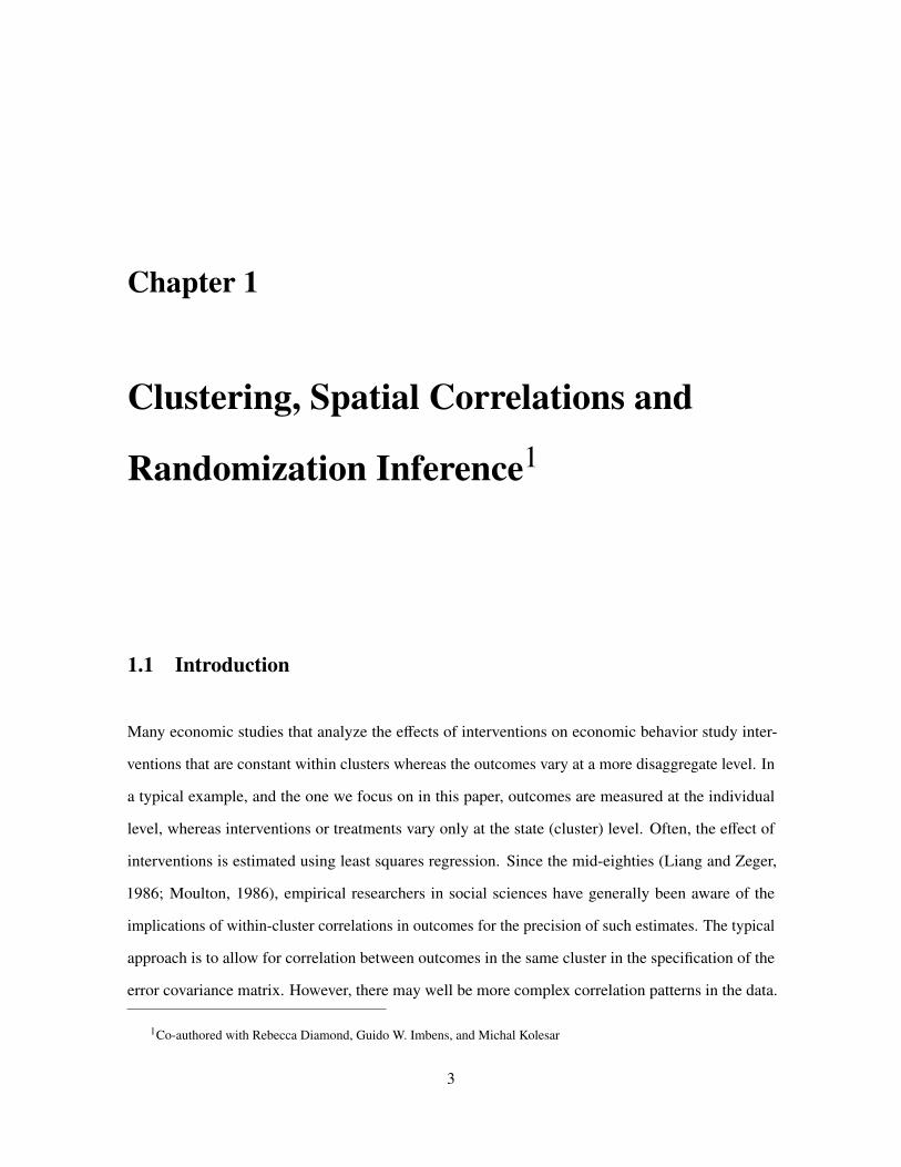
Figures 1.1 and 1.2 show the covariance functions for two choices of the bandwidth, h = 20 and

h = 50 miles, for the overall, within-state, and out-of-state covariances. The main conclusion from the

center panels of the figures is that within-state correlations decrease with distance. The lower panels

of the figures suggest that correlations for individuals in different states are non-zero, also decrease

with distance, and are of a magnitude similar to within-state correlations. Thus, these figures suggest

that the simple covariance model in (1.6) is not an accurate representation of the true covariance

10

structure.

Figure 1.1: Covariance of Demeaned Log(Earnings) by Distance Between Individuals

As a second piece of evidence we consider various parametric structures for the covariance matrix Ω(Z)

that generalize (1.6). At the most general level, we specify the following form for Ωi j(Z, γ):

Ωi j(Z, γ) =

σ2dist · exp(−α · d(Zi, Z j)) + σ2

D + σ2S + σ2

P + σ2ε if i = j,

σ2dist · exp(−α · d(Zi, Z j)) + σ2

D + σ2S + σ2

P if i , j, Pi = P j,

σ2dist · exp(−α · d(Zi, Z j)) + σ2

D + σ2S if Pi , P j, S i = S j,

σ2dist · exp(−α · d(Zi, Z j)) + σ2

D if S i , S j, Di = D j,

σ2dist · exp(−α · d(Zi, Z j)) if Di , D j.

(1.7)

11

Figure 1.2: Covariance of Demeaned Log(Earnings) by Distance Between Individuals

Beyond state level correlations this specification allows for correlations at the puma level (captured by

σ2P) and at the division level (captured by σ2

D). In addition we allow for spatial correlation as a smooth

function geographical distance, declining at an exponential rate, captured by σ2dist · exp(−α · d(z, z′)).

Although more general than the typical covariance structure allowed for, this model still embodies

important restrictions, notably that correlations do not vary by location. A more general model might

allow variances or covariances to vary directly by the location z, e.g., with correlations stronger or

weaker in the Western versus the Eastern United States, or in more densely or sparsely populated parts

of the country.

Table 1.3 gives maximum likelihood estimates for the covariance parameters γ given various re-

12

Table 1.3: Estimates for Clustering Variances for Demeaned Log Earnings

σ2ε σ2

D σ2S σ2

P σ2dis a LLH s.e.(β)

Min Wage NE/ENC

0.9388 0 0 0 0 0 1213298.1 0.0015 0.0015[0.0008 ]

0.9294 0 0.01610 0 0 0 1200407.0 0.0700 0.057[0.0008 ] [0.0018 ]

0.8683 0 0.0111 0.0659 0 0 1116976.4 0.0679 0.049[0.0008 ] [0.0029] [0.0022]

0.9294 0.0056 0.0108 0 0 0 1200403.1 0.0909 0.081[0.0008 ] [0.0020 ] [0.0020 ]

0.8683 0.0056 0.0058 0.0660 0 0 1116972.0 0.0805 0.0760[0.0008 ] [0.0033 ] [0.0021] [0.0021]

0.8683 0.0080 0.0008 0.0331 0.0324 0.0468 1603400.9 0.0860 0.0854[0.0008 ] [0.0049] [0.0012] [0.0021] [0.0030] [0.0051]

13

strictions, based on the log earnings data, with standard errors based on the second derivatives of

the log likelihood function. To put these numbers in perspective, the estimated value for α in the

most general model, α = 0.0293, implies that the pure spatial component, σ2dist · exp(−α · d(z, z′)),

dies out fairly quickly: at a distance of about twenty-five miles the spatial covariance due to the

σ2dist · exp(−α · d(z, z′)) component is half what it is at zero miles. The covariance of log earnings for

two individuals in the same puma is 0.080/0.948 = 0.084. For these data, the covariance between log

earnings and years of education is approximately 0.3, so the within-puma covariance is substantively

important, equal to about 30% of the log earnings and education covariance. For two individuals in the

same state, but in different pumas and ignoring the spatial component, the total covariance is 0.013. The

estimates suggest that much of what shows up as within-state correlations in a model that incorporates

only within-state correlations, in fact captures much more local, within-puma, correlations.

To show that these results are typical for the type of correlations found in individual level economic

data, we calculated results for the same models as in Table 1.3 for two other variables collected in the

census, years of education and hours worked. Results for those variables are reported in an earlier

version of the paper that is available online. In all cases puma-level correlations are a magnitude larger

than within-state, out-of-puma level correlations, and within-division correlations are of the same order

of magnitude as within-state correlations.

The two sets of results, the covariances by distance and the model-based estimates of cluster contribu-

tions to the variance, both suggest that the simple model in (1.6) that assumes zero covariances for

individuals in different states, and constant covariances for individuals in the same state irrespective of

distance, is at odds with the data. Covariances vary substantially within states, and do not vanish at

state boundaries.

Now we turn to the second question of this section, whether the magnitude of the correlations we

reported matters for inference. In order to assess this we look at the implications of the models for the

correlation structure for the precision of least squares estimates. To make this specific, we focus on

the model in (1.1), with log earnings as the outcome Yi, and Wi equal to an indicator that individual i

lives in a state with a minimum wage that is higher than the federal minimum wage in the year 2000.

14

This indicator takes on the value one for individuals living in nine states in our sample, California,

Connecticut, Delaware, Massachusetts, Oregon, Rhode Island, Vermont, Washington, and DC, and

zero for all other states in our sample (see Figure 1.3 for a visual impression). (The data come from the

website http://www.dol.gov/whd/state/stateMinWageHis.htm. To be consistent with the 2000 census,

we use the information from 2000, not the current state of the law.)

Figure 1.3: States with minimum wage higher than federal minimum wage

In the second to last column in Table 1.3, under the label “Min Wage,” we report in each row the

standard error for βols based on the specification for Ω(Z, γ) in that row. To be specific, if Ω = Ω(Z, γ)

is the estimate for Ω(Z, γ) in a particular specification, the standard error is

s.e.(βols) =

1

N2W2(1 −W)2

W

−1

′ (

ιN W)′

Ω(Z, γ)(ιN W

) W

−1

1/2

.

With no correlation between units at all, the estimated standard error is 0.002. If we allow only for

state level correlations, Model (1.6), the estimated standard error goes up to 0.080, demonstrating

the well known importance of allowing for correlation at the level that the covariate varies. There

are two general points to take away from the column with standard errors. First, the biggest impact

15

Figure 1.4: New England/East North Central States

on the standard errors comes from incorporating state-level correlations (allowing σ2S to differ from

zero), even though according to the variance component estimates other variance components are

substantially more important. Second, among the specifications that allow for σ2S , 0, however, there

is still a substantial amount of variation in the implied standard errors. Incorporating only σ2S leads to

a standard error around 0.0870, whereas also including division-level correlations (σ2D , 0) increase

that to approximately 0.090, an increase of 15%. We repeat this exercise for a second binary covariate,

with the results reported in the last column of Table 1.3. In this case the covariate takes on the value

one only for the New England (Massachusetts, Rhode Island, Connecticut, Vermont, New Hampshire)

and East-North-Central states (Wisconsin, Michigan, Illinois, Indiana, and Ohio, corresponding to

more geographical concentration than for the minimum wage states (see Figure 1.4). In this case the

impact on the standard errors of mis-specifying the covariance structure is even bigger, with the most

general specification leading to standard errors that are almost 50% bigger than those based on the

state-level correlations specification (1.6). In the next three sections we explore theoretical results that

provide some insight into these empirical findings.

16

1.4 Randomization Inference

In this section we consider a different approach to analyzing the distribution of the least squares

estimator, based on randomization inference (e.g., Rosenbaum, 2002). Recall the linear model

(1.1),

Yi = α+ β ·Wi + εi, with ε|W, Z ∼ N(0, Ω(Z)).

In Section 1.2 we analyzed the properties of the least squares estimator βols under repeated sampling.

To be precise, the sampling distribution for βols was defined by repeated sampling in which we keep

both the vector of treatments W and the location Z fixed on all draws, and redraw only the vector of

residuals ε for each sample. Under this repeated sampling thought-experiment, the exact variance of

βols is VM(W, Z) as given in Lemma 1.

It is possible to construct confidence intervals in a different way, based on a different repeated sampling

thought-experiment. Instead of conditioning on the vector W and Z, and resampling the ε, we can

condition on ε and Z, and resample the vector W. To be precise, let Yi(0) and Yi(1) denote the potential

outcomes under the two levels of the treatment Wi, and let Y(0) and Y(1) denote the corresponding

N-vectors. Then let Yi = Yi(Wi) be the realized outcome. We assume that the effect of the treatment

is constant, Yi(1) − Yi(0) = β. Defining α = E[Yi(0)], the residual is εi = Yi − α − β ·Wi. In this

section we focus on the simplest case, where the covariate of interest Wi is completely randomly

assigned, conditional on∑N

i=1 Wi = N1.

Assumption 2. Randomization

pr(W = w | Y(0), Y(1), Z) = 1/ N

N1

, for all w s.t.N∑

i=1

wi = N1.

Under this assumption we can infer the exact (finite sample) variance for the least squares estimator

for βols conditional on Z and (Y(0), Y(1)):

Lemma 2. Suppose that Assumption 2 holds and that the treatment effect Yi(1)−Yi(0) = β is constant

17

for all individuals. Then (i), βols conditional on (Y(0), Y(1)) and Z is unbiased for β,

E[βols

∣∣∣ Y(0), Y(1), Z]= β, (1.8)

and, (ii), its exact conditional (randomization-based) variance is

VR(Y(0), Y(1), Z) = V(βols

∣∣∣ Y(0), Y(1), Z)=

NN0 · N1 · (N − 2)

N∑i=1

(εi − ε)2 , (1.9)

where ε =∑N

i=1 εi/N.

Note that although the variance is exact, we do not have exact Normality, unlike the result in Lemma

1.

In the remainder of this section we explore two implications of the randomization perspective. First of

all, although the model and randomization variances VM and VR are exact if both Assumptions 1 and

2 hold, they differ because they refer to different conditioning sets. To illustrate this, let us consider

the bias and variance under a third repeated sampling thought experiment, without conditioning on

either W or ε, just conditioning on the locations Z and (N0, N1), maintaining both the model and the

randomization assumption.

Lemma 3. Suppose Assumptions 1 and 2 hold. Then (i), βols is unbiased for β,

E[βols

∣∣∣ Z, N0, N1]= β, (1.10)

(ii), its exact unconditional variance is:

VU(Z) =(

1N − 2

trace(Ω(Z)) −1

N · (N − 2)ι′NΩ(Z)ιN

)·

NN0 · N1

, (1.11)

and (iii),

VU(Z) = E [VR(Y(0), Y(1), Z)|Z, N0, N1] = E [VM(W, Z)|Z, N0, N1] .

For the second point, suppose we had focused on the repeated sampling variance for βols conditional

on W and Z, but possibly erroneously modeled the covariance matrix as constant times the identify

matrix, Ω(Z) = σ2 · IN . Under such a model one would have concluded that the exact sampling

18

distribution for βols would be

βols∣∣∣ W, Z ∼ N

(β,σ2 ·

NN0 · N1

), (1.12)

If the covariate was randomly assigned to the states, the normalized version of this variance would

converge to VR in (1.9). Hence, and this is a key insight of this section, if the assignment W is

completely random, and the treatment effect is constant, one can ignore the off-diagonal elements

of Ω(Z), and (mis-)specify Ω(Z) as σ2 · IN . Although the resulting variance estimator will not be

estimating the variance under the repeated sampling thought experiment that one may have in mind,

(namely VM(W, Z)), it leads to valid confidence intervals under the randomization distribution. The

result that the mis-specification of the covariance matrix need not lead to inconsistent standard errors

if the covariate of interest is randomly assigned has been noted previously. Greenwald (1983) writes:

“when the correlation patterns of the independent variables are unrelated to those across the errors, then

the least squares variance estimates are consistent.” Angrist and Pischke (2009) write, in the context

of clustering, that: “if the [covariate] values are uncorrelated within the groups, the grouped error

structure does not matter for standard errors.” The preceding discussion interprets this result formally

from a randomization perspective.

1.5 Randomization Inference with Cluster-level Randomization

Now let us return to the setting that is the main focus of the paper. The covariate of interest, Wi, varies

only between clusters (states), and is constant within clusters. Instead of assuming that Wi is randomly

assigned at the individual level, we now assume that it is randomly assigned at the cluster level. Let M

be the number of clusters, M1 the number of clusters with all individuals assigned Wi = 1, and M0 the

number of clusters with all individuals assigned to Wi = 0. The cluster indicator is

Cim = 1S i=m =

1 if individual i is in cluster/state m,

0 otherwise,

19

with C the N ×M matrix with typical element Cim. For randomization inference we condition on Z, ε,

and M1. Let Nm be the number of individuals in cluster m. We now look at the properties of βols over

the randomization distribution induced by this assignment mechanism. To keep the notation precise, let

W be the M-vector of assignments at the cluster level, with typical element Wm. Let Y(0) and Y(1) be

M-vectors, with m-th element equal to Ym(0) =∑

i:Cim=1 Yi(0)/Nm, and Ym(1) =∑

i:Cim=1 Yi(1)/Nm

respectively. Similarly, let ε be an M-vector with m-th element equal to εm =∑

i:Cim=1 εi/Nm, and let

ε =∑M

m=1 εm/M.

Formally the assumption on the assignment mechanism is now:

Assumption 3. (Cluster Randomization)

pr(W = w|Z = z) = 1/ M

M1

, for all w, s.t.M∑

m=1

wm = M1, and 0 otherwise.

We also make the assumption that all clusters are the same size:

Assumption 4. (Equal Cluster Size) Nm = N/M for all m = 1, . . . , M.

Lemma 4. Suppose Assumptions 3 and 4 hold, and the treatment effect Yi(1) − Yi(0) = β is constant.

Then (i), the exact sampling variance of βols, conditional on Z and ε, under the cluster randomization

distribution is

VCR(Y(0), Y(1), Z) =M

M0 ·M1 · (M − 2)

M∑m=1

(εm − ε

)2, (1.13)

(ii) if also Assumption 1 holds, then the unconditional variance is

VU(Z) =M2

M0 ·M1 · (M − 2) · N2 · (M · trace (C′Ω(Z)C) − ι′Ω(Z)ι) . (1.14)

The unconditional variance is a special case of the expected value of the unconditional variance in (1.5),

with the expectation taken over W given the cluster-level randomization. This result can be generalized

by allowing the random assignment to clusters to hold only conditional on covariates.

20

1.6 Variance Estimation Under Misspecification

In this section we present the main theoretical result in the paper. It extends the result in Section 1.4 on

the robustness of model-based variance estimators under complete randomization to the case where the

model-based variance estimator accounts for clustering, but not necessarily for all spatial correlations,

and that treatment is randomized at cluster level.

Suppose the model generating the data is the linear model in (1.1), with a general covariance matrix

Ω(Z), and Assumption 1 holds. The researcher estimates a parametric model that imposes a potentially

incorrect structure on the covariance matrix. Let Ω(Z, γ) be the parametric model for the error

covariance matrix. The model is misspecified in the sense that there need not be a value γ such that

Ω(Z) = Ω(Z, γ). The researcher then proceeds to calculate the variance of βols as if the postulated

model is correct. The question is whether this implied variance based on a misspecified covariance

structure leads to correct inference.

The example we are most interested in is characterized by a clustering structure by state. In that case

Ω(Z, γ) is the N × N matrix with γ = (σ2ε,σ

2S )′, where

Ωi j(Z,σ2ε,σ

2S ) =

σ2ε + σ2

S if i = j

σ2S if i , j, S i = S j,

0 otherwise.

(1.15)

Initially, however, we allow for any parametric structure Ω(Z, γ). The true covariance matrix Ω(Z)

may include correlations that extend beyond state boundaries, and that may involve division-level cor-

relations or spatial correlations that decline smoothly with distance as in the specification (1.7).

Under the (misspecified) parametric model Ω(Z, γ), let γ be the pseudo true value, defined as the

value of γ that maximizes the expectation of the logarithm of the likelihood function,

γ = arg maxγ

E

[−

12· ln (det (Ω(Z, γ))) −

12·Y′Ω(Z, γ)−1Y

∣∣∣∣∣ Z].

Given the pseudo true error covariance matrix Ω(γ), the corresponding pseudo-true model-based

21

variance of the least squares estimator, conditional on W and Z, is

VM(Ω(Z, γ), W, Z) =1

N2W2(1 −W)2

W

−1

′ (ιN W

)′Ω(Z, γ)

(ιN W

) W

−1

.

Because for some Z the true covariance matrix Ω(Z) differs from the misspecified one, Ω(Z, γ), it

follows that in general this pseudo-true conditional variance VM(Ω(Z, γ), W, Z) will differ from

the true variance VM(Ω(Z), W, Z). Here we focus on the expected value of VM(Ω(Z, γ), W, Z),

conditional on Z, under assumptions on the distribution of W. Let us denote this expectation by

VU(Ω(Z, γ), Z) = E[VM(Ω(Z, γ), W, Z)|Z]. The question is under what conditions on the specifi-

cation of the error-covariance matrix Ω(Z, γ), in combination with assumptions on the assignment

process, this unconditional variance is equal to the expected variance with the expectation of the

variance under the correct error-covariance matrix, VU(Ω(Z), Z) = E[VM(Ω(Z), W, Z)|Z].

The following theorem shows that if the randomization of W is at the cluster level, then solely

accounting for cluster level correlations is sufficient to get valid confidence intervals.

Theorem 1. (Clustering withMisspecified Error-CovarianceMatrix)

Suppose that Assumptions 1, 3, and 4 hold, and suppose that that Ω(Z, γ) is specified as in (1.15).

Then VU(Ω(Z, γ), Z) = VU(Ω(Z), Z).

This is the main theoretical result in the paper. It implies that if cluster level explanatory variables

are randomly allocated to clusters, there is no need to consider covariance structures beyond those

that allow for cluster level correlations. In our application, if the covariate (state minimum wage

exceeding federal minimum wage) were as good as randomly allocated to states, then there is no need

to incorporate division or puma level correlations in the specification of the covariance matrix. It is

in that case sufficient to allow for correlations between outcomes for individuals in the same state.

Formally the result is limited to the case with equal sized clusters. There are few exact results for the

case with variation in cluster size, although if the variation is modest, one might expect the current

results to provide some guidance.

In many econometric analyses researchers specify the conditional distribution of the outcome given

22

some explanatory variables, and ignore the joint distribution of the explanatory variables. The result in

Theorem 1 shows that it may be useful to pay attention to this distribution. Depending on the joint

distribution of the explanatory variables, the analyses may be robust to mis-specification of particular

aspects of the conditional distribution. In the next section we discuss some methods for assessing the

relevance of this result.

1.7 Spatial Correlation in State Averages

The results in the previous sections imply that inference is substantially simpler if the explanatory

variable of interest is randomly assigned, either at the unit or cluster level. Here we discuss tests

originally introduced by Mantel (1967) (see, e.g., Schabenberger and Gotway, 2004) to analyze

whether random assignment is consistent with the data, against the alternative hypothesis of some

spatial correlation. These tests allow for the calculation of exact, finite sample, p-values. To implement

these tests we use the location of the units. To make the discussion more specific, we test the random

assignment of state-level variables against the alternative of spatial correlation.

Let Ys be the variable of interest for state s, for s = 1, . . . , S , where state s has location Zs (the centroid

of the state). In the illustrations of the tests we use an indicator for a state-level regulation, and the

state-average of an individual-level outcome. The null hypothesis of no spatial correlation in the

Ys can be formalized as stating that conditional on the locations Z, each permutation of the values

(Y1, . . . , YS ) is equally likely. With S states, there are S ! permutations. We assess the null hypothesis

by comparing, for a given statistic M(Y, Z), the value of the statistic given the actual Y and Z, with

the distribution of the statistic generated by randomly permuting the Y vector.

The tests we focus on in the current paper are based on Mantel statistics (e.g., Mantel, 1967; Schaben-

berger and Gotway, 2004). These general form of the statistics we use is Geary’s c (also known as a

Black-White or BW statistic in the case of binary outcomes), a proximity-weighted average of squared

23

pairwise differences:

G(Y, Z) =S−1∑s=1

S∑t=s+1

(Ys − Yt)2· dst, (1.16)

where dst = d(Zs, Zt) is a non-negative weight monotonically related to the proximity of the states

s and t. Given a statistic, we test the null hypothesis of no spatial correlation by comparing the

value of the statistic in the actual data set, Gobs, to the distribution of the statistic under random

permutations of the Ys. The latter distribution is defined as follows. Taking the S units, with values for

the variable Y1, . . . , YS , we randomly permute the values Y1, . . . , YS over the S units. For each of the

S ! permutations g we re-calculate the Mantel statistic, say Gg. This defines a discrete distribution with

S ! different values, one for each allocation. The one-sided exact p-value is defined as the fraction of

allocations g (out of the set of S ! allocations) such that the associated Mantel statistic Gg is less than

or equal to the observed Mantel statistic Gobs:

p =1S !

S !∑g=1

1Gobs≥Gg. (1.17)

A low value of the p-value suggests rejecting the null hypothesis of no spatial correlation in the variable

of interest. In practice the number of allocations is often too large to calculate the exact p-value

and so we approximate the p-value by drawing a large number of allocations, and calculating the

proportion of statistics less than or equal to the observed Mantel statistic. In the calculations below we

use 10, 000, 000 draws from the randomization distribution.

We use six different measures of proximity. First, we define the proximity dst as states s and t sharing

a border:

dBst =

1 if s, t share a border,

0 otherwise.(1.18)

Second, we define dst as an indicator for states s and t belonging to the same census division of states

(recall that the US is divided into 9 divisions):

dDst =

1 if Ds = Dt,

0 otherwise.(1.19)

The last four proximity measures are functions of the geographical distance between states s and

24

t:

dGDst = −d (Zs, Zt) , and dαst = exp (−α · d (Zs, Zt)) (1.20)

where d(z, z′) is the distance in miles between two locations z and z′, and Zs is the latitude and

longitude of state s, measured as the latitude and longitude of the centroid for each state. We use

α = 0.00138, α = 0.00276, and α = 0.00693. For these values the proximity index declines by 50%

at distances of 500, 250, and 100 miles.

We calculate the p-values for the Mantel test statistic based on three variables. First, an indicator for

having a state minimum wage higher than the federal minimum wage. This indicator takes on the

value 1 in nine out of the forty nine states in our sample, with these nine states mainly concentrated in

the North East and the West Coast. Second, we calculate the p-values for the average of the logarithm

of yearly earnings. Third, we calculate the p-values for the indicator for NW and ENC states. The

results for the three variables and six statistics are presented in Table 1.4. All three variables exhibit

considerable spatial correlation. Interestingly the results are fairly sensitive to the measure of proximity.

From these limited calculations, it appears that sharing a border is a measure of proximity that is

sensitive to the type of spatial correlations in the data.

Table 1.4: p-values for Mantel Statistics, based on 10,000,000 draws and one-sided alternatives

Proximity −→ Border Divison −d(Zs, Zt) exp(−α · d(Zs, Zt))α = 0.00138 α = 0.00276 α = 0.00693

Minimum wage 0.0002 0.0032 0.0087 0.2674 0.0324 0.0033

Log wage 0.0005 0.0239 0.0692 0.0001 < 0.0001 < 0.0001

Education < 0.0001 0.0314 0.0028 < 0.0001 < 0.0001 < 0.0001

Hours Worked 0.0055 0.8922 0.0950 0.0243 0.0086 0.0182

Weeks Worked 0.0018 0.5155 0.1285 0.0217 0.0533 0.3717

25

1.8 A Small Simulation Study

We carried out a small simulation study to investigate the relevance of the theoretical results from

Section 1.6. In all cases the model was

Yi = α+ β ·Wi + εi,

with N = 2, 590, 190 observations to mimic our actual data. In our simulations every state has the

same number of individuals, and every puma within a given state has the same number of individuals.

We considered three distributions for Wi. In all cases Wi varies only at the state level. In the first case

Wi = 1 for individuals in nine randomly chosen states. In the second case Wi = 1 for the the nine

minimum wage states. In the third case Wi = 1 for the eleven NE and ENC states. The distribution

for ε is in all cases Normal with mean zero and covariance matrix Ω. The general specification we

consider for Ω is

Ωi j(Z, γ) =

σ2D + σ2

S + σ2P + σ2

ε if i = j,

σ2D + σ2

S + σ2P if i , j, Pi = P j,

σ2D + σ2

S if Pi , P j, S i = S j,

σ2D if S i , S j, Di = D j,

We look at two different sets of values for (σ2ε,σ

2P,σ2

S ,σ2D), (0.9294, 0, 0.0161, 0) (only state level cor-

relations) and (0.8683, 0.0056, 0.0058, 0.0660) (puma, state and division level correlations), motivated

by estimates in Section 1.3.

Given the data, we consider five methods for estimating the variance of the least squares estima-

tor βols, and thus for constructing confidence intervals. The first is based on the randomization

distribution:

VCR(Y(0), Y(1), Z) =M

M0 ·M1 · (M − 2)

M∑m=1

ˆε2m,

where ˆεm is the average value of the residual εi = Yi − αols − βols ·Wi over cluster m. The second, third

26

and fourth variances are model-based:

ˆmmvM(Ω(Z), W, Z) =1

N2 ·W2· (1 −W)2

(W − 1)(ιN W

)′Ω(Z)

(ιN W

) W

−1

,

using different estimates for Ω(Z). First we use an infeasible estimator, namely the true value for

Ω(Z). Second, we specify

Ωi j(Z, γ) =

σ2

S + σ2ε if i = j,

σ2S if i , j, S i = S j.

We estimate σ2P and σ2

S by maximum likelihood and plug that into the expression for the covariance

matrix. For the third variance estimator in this set of three variance estimators we specify

Ωi j(Z, γ) =

σ2D + σ2

S + σ2P + σ2

ε if i = j,

σ2D + σ2

S + σ2P if i , j, Pi = P j,

σ2D + σ2

S if Pi , P j, S i = S j,

σ2D if S i , S j, Di = D j,

and again use maximum likelihood estimates.

The fifth and last variance estimator allows for more general variance structures within states, but

restricts the correlations between individuals in different states to zero. This estimator assumes Ω is

block diagonal, with the blocks defined by states, but does not impose constant correlations within the

blocks. The estimator for Ω takes the form

ΩSTATA,i j(Z) =

ε2i if i = j,

εi · ε j if i , j, S i = S j,

0 otherwise,

27

leading to

VS T AT A =1

N2 ·W2(1 −W)2

· (W − 1)(ιN W

)′ΩSTATA(Z)

(ιN W

) W

−1

.

This is the variance estimator implemented in STATA.

Table 1.5: Size of t-tests (in %) using different variance estimators (500,000 draws).

Treatment type Random Min. Wage NE/ENC

Shock type S S PD S S PD S S PD

VCR(Y(0), Y(1), Z) 5.6 5.6 5.6 16.2 5.6 26.3VM(Ω(Z), W, Z) 5.0 5.0 5.0 5.0 5.0 5.0VM(Ω(σ2

ε , σ2S ), W, Z) 6.1 6.1 6.1 17.1 6.1 27.2

VM(Ω(σ2ε , σ

2P, σ2

S , σ2D), W, Z) 6.1 6.5 5.7 9.0 5.4 13.8

Stata 7.6 7.6 8.5 18.5 7.7 30.4

In Table 1.5 we report the actual level of tests of the null hypothesis that β = β0 with a nominal level

of 5%. First consider the three columns with random assignment of states to the treatment. In that

case all variance estimators lead to tests that perform well, with actual levels between 4.9 and 7.6%.

Excluding the STATA variance estimator the actual levels are below 6.4%. The key finding is that

even if the correlation pattern involves pumas as well as divisions, variance estimators that ignore the

division level correlations do very well.

When we do use the minimum wage states as the treatment group the assignment is no longer

completely random. If the correlations are within state, all variance estimators still perform well.

However, if there are correlations at the division level, now only the variance estimator using the true

variance matrix does well. The estimator that estimates the division level correlations does best among

the feasible estimators, but because the data are not informative enough about these correlations to

precisely estimate the variance components even this estimator exhibits substantial size distortions.

The same pattern, but even stronger, emerges with the NE/ENC states as the treatment group.

28

1.9 Conclusion

In empirical studies with individual level outcomes and state level explanatory variables, researchers

often calculate standard errors allowing for within-state correlations between individual-level outcomes.

In many cases, however, the correlations may extend beyond state boundaries. Here we explore the

presence of such correlations, and investigate the implications of their presence for the calculation

of standard errors. In theoretical calculations we show that under some conditions, in particular

random assignment of regulations, correlations in outcomes between individuals in different states

can be ignored. However, state level variables often exhibit considerable spatial correlation, and

ignoring out-of-state correlations of the magnitude found in our application may lead to substantial

underestimation of standard errors.

In practice we recommend that researchers explicitly explore the spatial correlation structure of both

the outcomes as well as the explanatory variables. Statistical tests based on Mantel statistics, with

the proximity based on shared borders, or belonging to a common division, are straightforward to

calculate and lead to exact p-values. If these test suggest that both outcomes and explanatory variables

exhibit substantial spatial correlation, we recommend that one should explicitly account for the spatial

correlation by allowing for a more flexible specification than one that only accounts for state level

clustering.

29

Chapter 2

Optimal Stratification in Randomized

Experiments

2.1 Introduction

Experimenters often face the following situation: they are ready to assign treatment to some subset

of units in an experimental group, they have a rich amount of information about each unit –from a

baseline survey, a pilot, or administrative records– and they would like to ensure that the treatment

and control groups are similar with respect to these variables. They can pick one or two variables and

stratify on those, making those variables more balanced after randomization, but what about the rest?

Furthermore, on which of the variables should they stratify?

Let’s take for example state prison administrators who want to test interventions that reduce recidivism.

Their goal is to have released inmates complete a successful twelve-month post-release supervision

regime1. For the experiment, they have drawn a sample of sixty inmates with six months remaining on

their sentences, thirty of whom will receive an intervention. Detailed state administrative records have

1Presently, a large portion of released inmates re-enter prison because of technical violations during the twelve monthsof post-release supervision.

30

been kept for each inmate starting from the point of arrest. At the beginning of the study, researchers

have a large set of baseline variables: past criminal record, prison behavior, family history, and

education.

With only sixty units in the experiment, complete random assignment may produce treatment and

control groups that are not comparable2. Researchers in our example have thus decided on a matched-

pair randomization; they will put the sixty inmates into thirty pairs, and one of the two people in

each pair will be assigned treatment. This paper shows that an optimal way to choose the thirty

pairs is to (1) use all available baseline information to predict whether each inmate will successfully

complete post-release supervision, (2) rank inmates according to this prediction, and (3) match pairs

by assigning the two highest ranked inmates to one pair, the next two highest to the second pair, and so

on until the two lowest ranked inmates are assigned to the last pair. This will require data to estimate

prediction functions. In this example, the estimation can be done using information from previous

inmate cohorts.

This paper considers the gain in efficiency3 from effective stratification. We show that stratifying, in the

case of matched pairs, leads to significant efficiency gains, that gains will be large if baseline variables

are good predictors of the outcome of interest, and that it is optimal to stratify on the conditional

expectation of the outcome given baseline variables. Simulations show that the gain in efficiency is

comparable to having controlled for covariates in the analysis after randomization. That is, given a set

of covariates X, matching on predictions based on X and estimating the difference in means ex-post

gives estimators with mean squared error of the same size as performing a complete randomization

and controlling for X with regression ex-post. This paper focuses on the difference in means since this

estimate is typically the key finding from a randomized experiment (Angrist and Pischke, 2010). Thus

this method is helpful to modern researchers who, according to Angrist and Pischke (2010) “often

2More precisely, a significant portion of treatment assignments may produce groups that, absent the treatment, expectto have significant differences in the average outcome, and that the magnitude of these differences will be large relative toexpected treatment effect sizes.

3Stratification is generally done for one of two reasons: to estimate heterogeneous treatment effects across strata or tomake standard errors smaller. This paper considers the latter.

31

prefer simpler estimators though they might be giving up asymptotic efficiency” (p. 12). This paper

keeps the estimator simple and shows how optimal matching can regain lost efficiency via stratification.

Simple estimators also aid in the delivery of research findings to policy makers. Dean Karlan offers

the following on scaling up interventions:

How do we make it easy for government to make the right choices? How do we makeit easy for N.G.O.s to choose the right thing? ... You can, the fact that you can put upa simple bar chart makes it easy for people to get it. Okay, treatment is here, control isthere, I see the impact. The minute you have really fancy econometrics with lots of GreekLetters, you are not making it easy for policy makers to understand and decipher what thelessons are from a research paper. (Karlan, 2013)

The method used here is especially useful when the number of baseline covariates is very large, since the

conditional expectation function collapses multi-dimensional covariates onto a single dimension. This

gives experimenters a way to use big data (possibly more covariates than the number of experimental

units) ex-ante and maintain simple post-experiment inference techniques. It leverages both the large

amount of available baseline information and the tools of predictive analysis (Hastie, Tibshirani, and

Friedman 2009) that are increasingly being developed in the field of statistical learning to inform

experimental design.

Large detailed datasets are becoming increasingly available to experimenters. Beyond the example

above, experimenters partnered with private firms may be able to use the firm’s administrative records

to inform the design of randomized trials. For example, there have been trials to measure the effects

of working from home on productivity (Bloom et al., 2013), peer saving habits on contributions

to retirement plans (Beshears et al., 2011), and streamlined college application materials on high-

performing, low-income student enrollment at selective colleges (Hoxby and Turner, 2013).

Whether the experiment is set at a Chinese travel agency (Bloom et al., 2013), an American manu-

facturing firm (Beshears et al., 2011), or a non-profit entrance exam association (Hoxby and Turner,

2013), rich information is increasingly available not only for the units in the experiment but also for

the population from which these units are drawn and for comparable past populations. In the public

sphere, Medicare and Medicaid programs store information on services to participants, and public

32

school districts keep detailed records of student academic outcomes, teachers, and classrooms. These

agencies have recently allowed academic researchers to evaluate programs in cases where lotteries

have been used for limited numbers of program spots (Finkelstein et al. 2012, Angrist et al. 2013).

It is not implausible that in the future, researchers will be brought in earlier and have input in the

design of randomizations explicitly to increase the amount of information gleaned from these program

evaluations (e.g. Kane et al., 2013).

The main worry with using many control variables in the analysis after an experiment is that the data

generating process will be unknown, and researchers have a variety of ways to add controls. Controls

are often tried in many specifications. With a large number of specifications, experimenters may

report only those with significant results. A set of controls, X, can be outlined in a pre-analysis plan

(Casey et al., 2011). But specification searches can still be done by selectively including or excluding

controls not in X. Even within X, linear models can be specified in X1, .., Xk, X1, X21 .., Xk, X2

k ,

X1, X21 , X1 · X2, ..., X2

k , or any other set of linear controls that take the elements of X as primitive

variables. In contrast, the method in this paper suggests a unique set of controls, the set of pair

indicators. While an analysis can include other additional controls, perhaps as robustness checks4, a

report of the difference in means with standard errors of correct size will be expected and our set of

controls provide exactly that for the difference in means estimator.

Another worry is that researchers will look for treatment effects across many outcomes. Optimizing

the randomization with respect to one outcome allows researchers to credibly signal the outcome of

interest prior to the experiment5. If there is interest in a variety of related outcomes then researchers

could designate a broad index as the main outcome of the experiment (e.g. Ludwig et al., 2012).

The next section formalizes the main result. Section 3 describes how the method can be used in

practice. Section 4 will go over the ex-post analysis and show how standard methods apply. Section

5 will review model selection methods used in prediction and how they have been used here. To

4For example matching has been coupled with regression adjustment (Rubin, 1973).

5Casey et al., (2011) discuss the practice of having experiment pre-analysis plans and how these plans add credibility toprogram analyses by designating controls and outcomes at the design stage of the experiment.

33

demonstrate those methods, section 6 revisits a set of field-experiment based simulations by Bruhn and

McKenzie (2011) and shows how experimenters could have used information available at baseline to

estimate conditional expectation functions of outcomes given baseline covariates. Section 7 turns to

the literature and compares this method to others.

2.2 Main Result

Set-up

We first lay out the primitives of the experiment. The subjects in the experiment are sampled from an

underlying population. For each subject, we observe a vector of covariates before the experiment is

conducted. After the experiment we observe a real valued outcome. The outcome we observe will

depend on whether or not the individual was treated. We can think of each individual having a pair of

potential outcomes that correspond to the two different exposures to treatment. We refer to exposure

to treatment as treatment, and withholding of the treatment or exposure to a placebo as control. This

set of primitives is commonly referred to as Rubin’s causal model. Within this framework we are

interested in the average causal effect of treatment on the outcome.

A key condition will be that, for every individual, treatment assignment is independent of potential

outcomes. Pairing experimental units will not change this independence. What pairing changes is the

correlation of treatment across individuals. More explicitly, it makes treatment assignment perfectly

negatively correlated between pairs. Across pairs treatment assignment remains independent.

Throughout we will consider the following setup.

Assumption 1

1. Sampling from a population: We randomly sample N units i = 1, .., N, where N is even, from

some population. Units of observation are characterized by a vector of covariates Xi ∈ RK as

well as a potential outcome function Yi(·) : 0, 1 7→ R. At this point only the covariate column

vector Xi is observed.

34

2. Treatment assignment: We assign treatment Ti to unit i as a function of the matrix of covariates

X = (X′i , ..., X′N)′. Let Yi(1), Yi(0) y T j | X ∀i, j.

3. Realization of outcomes: The observed outcome is the potential outcome corresponding to the

assigned treatment level: Yi = Yi(Ti)

Note that the second part of Assumption 1.2 encompasses SUTVA, the “stable unit treatment value

assumption”, (Angrist et al., 1996)). SUTVA states that given individual treatment assignment,

potential outcomes are independent of other treatment assignments. More formally θi y T\Ti.

Treatment Effects, Average Treatment Effect (ATE), and Prognostic Score

Our parameter of interest, or target, is the population average causal effect of treatment. Note

that in drawing notation for this parameter we are implicitly assuming this population moment exists.

Individual causal (treatment) effects are defined as differences in individuals’ potential outcomes. These,

of course, are unobservable since only one potential outcome per individual is ever observed.

We can form expectations for each potential outcome conditional on the observed covariates. At

the introduction of a new treatment there exists information about how outcomes evolve absent the

treatment. This is formalized by the prognostic score, i.e. the conditional expectation of the outcome

in the absence of treatment. The prognostic score tells us what is expected, or predicted, to happen

in a world where treatment does not yet exist. Errors from these predictions encompass unobserved

determinants of the outcome.

Definition 1

1. Denote the average treatment effect (ATE) θ ≡ E(Yi(1) − Yi(0)).

2. For unit i denote the treatment effect θi ≡ Yi(1) − Yi(0), i = 1, ..., N.

3. Denote the sample average treatment effect (SATE) θS AT E ≡1N

∑Ni=1 θi.

4. Denote the prognostic score r(Xi) ≡ E (Yi(0)∣∣∣Xi) and let εi ≡ Yi(0) − r(Xi).

35

Now we can describe the relationships between potential outcomes, treatment, prognostic score, and

prediction error. The potential outcome, absent treatment, is the sum of the prognostic score and

prediction error. The addition of a treatment effect gives the potential outcome under exposure to

treatment. The observed outcome is given by the sum of prognosis, prediction error, and, if treated,

treatment effect. More formally, Definition 1 gives us that

Yi(0) = r(Xi) + εi

Yi(1) = θi + r(Xi) + εi

Yi = Tiθi + r(Xi) + εi

Re-indexing and matched pairs

The paired nature of the experimental units makes it useful for reorder their index i so that units in the

same pair are adjacent to each other. This will allow us to discuss a particular pair by referring to the

individuals’ index. Here we do this so that the kth pair is units 2k − 1 and 2k. This also allows us to

parsimoniously describe treatment assignments.

Let the index i be re-ordered in a matched pairs randomization scheme where Ti = 1 − Ti+1 for i odd,

and Ti ∼iid Bernoulli(1/2) for i odd.

With units and treatment assignments as described above we can establish notation for within pair

differences. The average of within pair differences is the difference of averages between treatment and

control units, our statistic of interest.

Definition 2 (Estimator and within pair differences)

1. Denote the within pair differences

Dk = T2k−1 [Y2k−1(1) − Y2k(0)] + (1 − T2k−1) [Y2k(1) − Y2k−1(0)]

for k = 1, ..., N2

36

2. Denote the sample average D ≡ 2N

∑ N2k=1 Dk.

Proposition 1 Unbiasedness: Given Assumption 1 and taking expectations over the distribution

of treatment assignments, then D is an unbiased estimator of the sample average treatment effect,

θS AT E .

proof: Given assumption 1 and definitions 1 and 2, by iterated expectations

E(Dk|Y(1), Y(0)) = E(Dk|Yi(1), Yi(0))

=12[Y2k−1(1) + Y2k(1) − Y2k−1(0) − Y2k(0)]

=12[θ2k−1 + θ2k]

By definition 2

E[D|Y(1), Y(0)] =2N

N2∑

k=1

12[θ2k−1 + θ2k]

=1N

N∑i=1

θi

= θS AT E

Corollary 1 It follows, by taking expectations over the distribution of X described in Assumption 1.1,

that D is an unbiased estimator of the average treatment effect. It further follows, by taking expectations

over the conditional distribution of potential outcomes holding covariates fixed, that D is an unbiased

estimator of the conditional average treatment effect, 1N

∑Ni=1 E[Yi(1) − Yi(0)|X].

Now we can evaluate the variance of this statistic as follows.

By Definition 2 we have

var(D|X

)=

(2N

)2

N2∑

k=1

var(Dk|X) +∑h,k

cov(Dk, Dh|X)

(2.1)

37

Next, we find expressions for each component of the sum in equation 2.1

Proposition 2: If Assumption 1 holds, θi|X, ε are independent, and E(θi|X, ε) = θ then

var(Dk|X) =12[var(θ2k−1|X) + var(θ2k|X)] (2.2)

+ var(ε2k−1|X) + var(ε2k|X)

+ [r(X2k−1) − r(X2k)]2, ∀k,

and

cov(Dk, Dh|X) = 0, ∀h , k. (2.3)

These give

var(D|X)(2N

)2 =N∑

i=1

[12

var(θi|X) + var(εi|X)]+

N2∑

k=1

(r(X2k−1) − r(X2k))2 (2.4)

proof: Given in Appendix.

The main result is that of all possible ways to pick pairs the optimal way depends on covariates only

through their prediction. First we need to formally define a pairing and relate it to our potential

outcome notation.

Definition 3 (Pairing)

For N even, a pairing, p, is a permutation of the set 1, ..., N. The pairs defined by p are p(2k −

1), p(2k)N2k=1. Two pairings, p and p′, are different if and only if there exist k and h s.t. p(2k −

1), p(2k) ∩ p′(2h − 1), p′(2h) , ∅, and p(2k − 1), p(2k) , p′(2h − 1), p′(2h).

This definition gives an equivalence relation on the set of permutations, i.e. two pairings are equivalent

if at least one experimental unit assigned differently between pairings. The set of equivalence classes

produced by this relation is what we call the set of pairings. Our goal is to find the pairing that

minimizes equation 2.1.

38

Proposition 3: Let ri ≡ r(Xi) ∀i, and let r(1), r(2), ..., r(N) denote the order statistics of r1, r2, ..., rN . If

Assumption 1 holds and θi|X, ε are i.i.d with E(θi|X, ε) = θ, then var(D|X) is minimized by the pairing

(1), (2), ..., (N). This pairing is a permutation of 1, .., N. The pairs are (2k − 1), (2k)N2k=1.

proof:

By Proposition 1 var(D|X) depends on pairs only via

N2∑

k=1

r(2k−1)r(2k).

So we must showN2∑

k=1

r(2k−1)r(2k) ≥

N2∑

k=1

rp(2k−1)rp(2k)

for all other pairings p.

Suppose for the purposes of deriving a contradiction that p is maximal for

N2∑

k=1

rp(2k−1)rp(2k)

and there exists subset a1, a2, a3, a4 ⊆ r1, ..., rN where a1 ≤ a2 ≤ a3 ≤ a4 and are not paired in

order under p. If a1 = a2 = a3 = a4 then it is not possible to pair the subset out of order. Likewise

it is not possible if a1 < a2 = a3 = a4 or a1 = a2 = a3 < a4. Suppose a1 = a2 < a3 = a4,

then it must be that under p the pairs are a1, a3 and a2, a4. Now consider a1a3 + a2a4, we will

show that a1a2 + a3a4 is larger and thus p is not maximal. We have a1a3 + a2a4 = 2a1a3 and

a1a2 + a3a4 = a21 + a2

3 . Suppose for contradiction that a21 + a2

3 ≤ 2a1a3 ⇐⇒ a21 + a2

3 − 2a1a3 ≤ 0,

but a21 + a2

3 − 2a1a3 = (a1 − a3)2 > 0. Thus it must be that a1, a2, a3, a4 has at least three distinct

elements.

• Case 1: a1 = a2 < a3 < a4. Under p the pairs must be a1, a3 and a2, a4 since a1 = a2. Under

p we obtain a1a3 + a2a4 = a1a3 + a1a4 compared to the alternative pairing a1, a2 and a3, a4

where we obtain a1a2 + a3a4 = a1a1 + a3a4 . Now suppose a1a3 + a1a4 ≥ a1a1 + a3a4 ⇐⇒

39

a1(a3 − a1) ≥ (a3 − a1)a4 ⇐⇒ a1 ≥ a4 since a3 > a1. But a1 < a4 by transitivity.

• Case 2: a1 < a2 = a3 < a4. Under p it must be a1, a4 and a2, a3 are paired. Under p we

obtain a1a4 + a2a2 whereas under the alternative a1, a2 and a3, a4 we obtain a1a2 + a2a4.

Now suppose a1a4 + a2a2 ≥ a1a2 + a2a4 ⇐⇒ a1(a4 − a2) ≥ a2(a4 − a2) ⇐⇒ a1 ≥ a2, but

a1 < a2.

• Case 3: a1 < a2 < a3 = a4. Under p it must be that a1, a3 and a2, a4 are paired and we

obtain a1a3 + a2a3. Consider the alternative a1, a2 and a3, a4 where we obtain a1a2 + a3a3.

Suppose a1a3 + a2a3 ≥ a1a2 + a3a3 ⇐⇒ a1(a3 − a2) ≥ a3(a3 − a2) ⇐⇒ a1 ≥ a3, but

a3 > a1.

• Case 4: a1 < a2 < a3 < a4. Under p either a1 is paired with a3 or it is paired with a4. First, say

a1 and a3 are paired. Then we obtain a1a3 + a2a4. Let us compare that to a1a2 + a3a4. Suppose

a1a3 + a2a4 ≥ a1a2 + a3a4 ⇐⇒ a1(a3 − a2) ≥ a4(a3 − a2) ⇐⇒ a1 ≥ a4 a contradiction.

Instead say a1 and a4 are paired under p, then we obtain a1a4 + a2a3. Let us compare that to

a1a2 + a3a4. Suppose a1a4 + a2a3 ≥ a1a2 + a3a4 ⇐⇒ a1(a4 − a2) ≥ a3(a4 − a2) ⇐⇒ a1 ≥

a3, a contradiction.

Remarks Use empirical process notation: En[ f (ωi)] ≡1n∑n

i=1 f (ωi). Proposition 2 gives

N2

var(D|X) = EN [var(θi|X)] + 2EN [var(εi|X)] + E N2[(r(X2k−1) − r(X2k))

2] (2.5)

where the first two terms of this equation are irreducible error, and

E N2[(r(X2k−1) − r(X2k))

2]

40

is the error from within pair differences in r(Xi). If pairs do not match on the vectors Xi, but all pairs

match on the scalars r(Xi) then E N2[(r(X2k−1) − r(X2k))2] = 0, and equation 2.5 would only involve

irreducible error. This provides some intuition for this paper’s main results.

Other than Assumption 1 the proof of optimality required that treatment effects be independent of

(X, ε). A requirement, like this one, restricting the relationship between the conditional expectations of

potential outcomes is necessary for matching based on the prognostic score to be optimal. Consider the

following counter example where we do away with this type of requirement and allow E(Yi(1)|Xi = x)

and E(Yi(0)|Xi = x) to be unrestricted. Let potential outcomes be deterministic functions of a

univariate X, and let X take on the following values in a sample of four. The data could come from

four draws from the functions in Figure 2.1.

Table 2.1: Counter example where treatment effect not independent of (X, ε)

E(Yi(1)|xi) E(Y(0)i|xi) xi i1 1 1 14 2 2 29 3 3 32 4 4 4

The assumptions in Propositions 2 and 3 imply that the average treatment effect conditional on

covariates is constant for all values of the potential outcomes. In this counter example, that would

require the graphs in Figure 2.1 to differ by at most a vertical shift. In this deviation from that

assumption the optimal pairing depends on more than the order given by either conditional expectation

function.

Pairing on the prognostic score would pair units 1, 2 and 3, 4, and Var(D|X) would be 52/16. Pairs

matched on the predicted outcome for treatment would give 1, 4 and 2, 3 with Var(D|X) of 37/16.

The optimal pairs in this case are 1, 3 and 2, 4, they give Var(D|X) of 36/16.

2.2.1 General solution to the matching problem

Without making any assumptions we have the following formula for the variance:

41

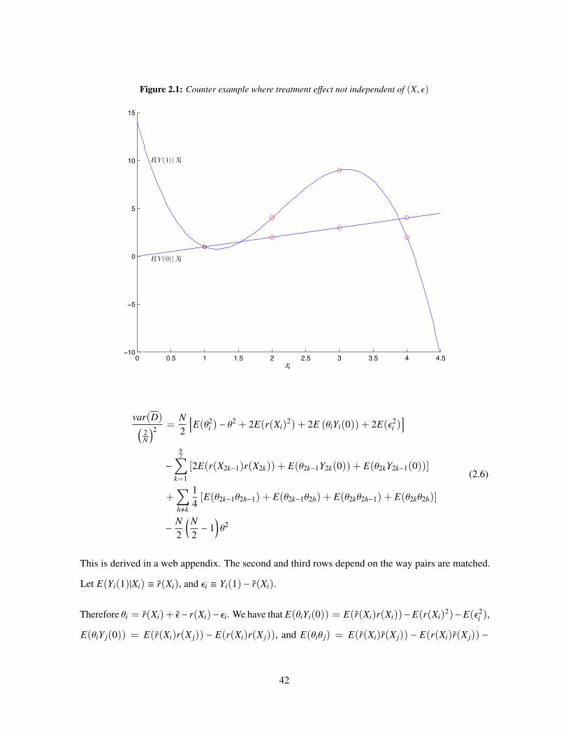
Figure 2.1: Counter example where treatment effect not independent of (X, ε)

0 0.5 1 1.5 2 2.5 3 3.5 4 4.5−10

−5

0

5

10

15Exampl e: Esti mates of E(Y(0) |X) and E(Y(1) |X)

xi

E(Y (0) |X)

E(Y (1) |X)

var(D)(2N

)2 =N2

[E(θ2

i ) − θ2 + 2E(r(Xi)

2) + 2E (θiYi(0)) + 2E(ε2i )

]

−

N2∑

k=1

[2E(r(X2k−1)r(X2k)) + E(θ2k−1Y2k(0)) + E(θ2kY2k−1(0))]

+∑h,k

14[E(θ2k−1θ2h−1) + E(θ2k−1θ2h) + E(θ2kθ2h−1) + E(θ2kθ2h)]

−N2

(N2− 1

)θ2

(2.6)

This is derived in a web appendix. The second and third rows depend on the way pairs are matched.

Let E(Yi(1)|Xi) ≡ r(Xi), and εi ≡ Yi(1) − r(Xi).

Therefore θi = r(Xi)+ ε − r(Xi)− εi. We have that E(θiYi(0)) = E(r(Xi)r(Xi))−E(r(Xi)2)−E(ε2i ),

E(θiY j(0)) = E(r(Xi)r(X j)) − E(r(Xi)r(X j)), and E(θiθ j) = E(r(Xi)r(X j)) − E(r(Xi)r(X j)) −

42

E(r(Xi)r(X j)) + E(r(Xi)r(X j)). Each of which are functions of X. Since the set of possible matches

is finite then for every possible realization of X optimization of equation 6 can be done by exhaustive

search over this set.

2.3 Matching in Practice

In practice the conditional expectation function–also referred to as the ‘prognosis score’ (Hansen,

2008)–is not known and will have to be estimated with data. This data can come from any sample

from the same population, for example a previous experiment, a rich baseline survey, an existing

observational study, or administrative data. This initial prediction can be based on many baseline

covariates. Since we will be using covariates to predict the outcome of interest, the goal is to use

them to make predictions with the best out of sample performance. To this end there are many

model selection procedures available, such as, AIC, BIC, Lasso, or ridge regression. This paper

provides some guidance on how to estimate the best predictors in the examples and compares their

performance.

Figure 2.2 shows each of the steps present in the matching procedure. The process starts with collection

of baseline covariates for the units in the experiment, in addition to collection of auxiliary (training)

covariates and outcome data from the same population. Next the training data is used to estimate a

prediction function. This function, coupled with the baseline covariates from the experiment group

form the procedure’s predicted outcomes. Matched pairs are based on these predictions. The pair

assignments are then operationalized as a set of pair indicators. Next, randomization produces a

treatment variable. After the experiment is conducted, an outcome variable is measured. The analysis

of this experiment, however, will use just the pair indicators, outcome, and treatment variable.

To build intuition for the procedure and to draw important distinctions, it is useful to compare the

present method with well known propensity score methods. In practice, the two steps for optimal

matched pairs randomization are analogous to matching procedures in observational studies based on

the propensity score (Rubin, 1983). In the first step, rather than estimating a propensity score (which

43

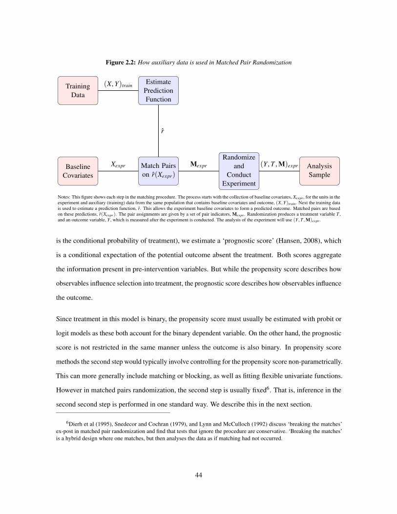
Figure 2.2: How auxiliary data is used in Matched Pair Randomization

TrainingData

BaselineCovariates

EstimatePredictionFunction

Match Pairson r(Xexpr)

Randomizeand

ConductExperiment

AnalysisSample

(X, Y)train

Xexpr

r

Mexpr (Y , T , M)expr

Notes: This figure shows each step in the matching procedure. The process starts with the collection of baseline covariates, Xexpr , for the units in theexperiment and auxiliary (training) data from the same population that contains baseline covariates and outcome, (X, Y)train. Next the training datais used to estimate a prediction function, r. This allows the experiment baseline covariates to form a predicted outcome. Matched pairs are basedon these predictions, r(Xexpr). The pair assignments are given by a set of pair indicators, Mexpr . Randomization produces a treatment variable T ,and an outcome variable, Y , which is measured after the experiment is conducted. The analysis of the experiment will use (Y , T , M)expr .

is the conditional probability of treatment), we estimate a ‘prognostic score’ (Hansen, 2008), which

is a conditional expectation of the potential outcome absent the treatment. Both scores aggregate

the information present in pre-intervention variables. But while the propensity score describes how

observables influence selection into treatment, the prognostic score describes how observables influence

the outcome.

Since treatment in this model is binary, the propensity score must usually be estimated with probit or

logit models as these both account for the binary dependent variable. On the other hand, the prognostic

score is not restricted in the same manner unless the outcome is also binary. In propensity score

methods the second step would typically involve controlling for the propensity score non-parametrically.

This can more generally include matching or blocking, as well as fitting flexible univariate functions.

However in matched pairs randomization, the second step is usually fixed6. That is, inference in the

second second step is performed in one standard way. We describe this in the next section.

6Dierh et al (1995), Snedecor and Cochran (1979), and Lynn and McCulloch (1992) discuss ‘breaking the matches’ex-post in matched pair randomization and find that tests that ignore the procedure are conservative. ‘Breaking the matches’is a hybrid design where one matches, but then analyses the data as if matching had not occurred.

44

2.4 Inference in Matched Pair Randomization

After randomization, both frequentist inference and randomization inference depend only on the actual

strata chosen and not on estimated predicted values. Covariates are used to form predictions which

are then used to choose pairs. Ex-post analysis is done conditionally on the chosen pairs; thus it is

unaffected by the process used to pick pairs. However, so long as good predictors of the outcome are

used, significant gains in efficiency will most likely be realized.

A standard way to obtain the difference in means estimator is from the following linear regression

model (Duflo et al., 2006),

E(Yi j|Ti j, M j) = α+ βTi j + δ jM j (2.7)

where i indexes individuals, j indexes pairs, Ti j is a treatment indicator, and M j is a pair indica-

tor.

Frequentist inference can be done using either the standard or robust estimates of the least squares

variance. In the case of matched pairs, there is also another procedure available, i.e. the paired

difference test (Rubin, 1973). The simplest way to think of the paired t-test is to construct within pair

differences, D j ≡ Y1 j − Y2 j (indexed so that the first unit is treated). This gives one difference for

each pair. The rest of the procedure amounts to estimating the mean with the sample average of the

differences, D = 1n∑

j D j, where n is the number of pairs. Standard errors for the test come from the

appropriately normalized sample variances of the differences, SE=√

1n

1n−1

∑j(D j − D)2. A t-statistic,

D/SE, is formed and compared to a critical value from the t-distribution with n− 1 degrees of freedom.

The test can be justified either asymptotically given a central limit theorem holds or in finite samples

with the assumption of normal errors.

Thus given a matched pair randomization one can view the data as a set of N outcome measurements

from the experimental units, where N/2 have been treated. One can then proceed with analysis by

regressing the outcome on a treatment indicator alongside a set of N/2 pair indicators. Alternatively

one can view the data as a set of n = N/2 within pair differences wherein the statistician is estimating

45

the simple mean of the n within pair differences7.

Randomization inference can also be conducted ex-post. The method, in general, considers a test

statistic and a sharp null hypothesis. The test statistic is evaluated at all possible counter-factual

assignments that could have been realized by the experiment. A sharp null hypothesis then specifies

exactly what the treatment effect is for every experimental unit and allows counter-factual potential

outcomes to be computed for every unit. It is commonly the case that the sharp null hypothesizes

exactly zero effect of treatment for every unit. Under this null both potential outcomes are identical for

each unit, so that outcomes would be the same under any treatment assignment. In a matched pairs

experiment with N/2, pairs there would be 2N/2 possible assignments and the distribution of a test

statistic can be computed over this distribution. Inference would then be conducted by comparing the

value of the statistic to the proportion of more extreme values in the underlying distribution.

2.4.1 Treatment Compliance

Often in experiments not all treatment assignments are followed. For example experimenters may

randomize admission into a work-training program, but not all admitted applicants may enroll. Fur-

thermore, some applicants who were randomized out of the program may be admitted after reapplying.

In these cases one can use the original treatment assignments to estimate the effect of Intent To

Treat (ITT) by redefining Ti in this model’s set-up to denote treatment assignment instead of actual

treatment.

2.5 Model Selection and Prediction Methods

In this section we present and discuss four model selection methods: AIC, the Akaike Information

Criterion; BIC, Bayes’ Information Criterion; Lasso, the least absolute shrinkage and selection

7Two interesting but non critical observations are described in appendix A.

46

operator; and Ridge regression. This paper uses each of these four methods to select models in

simulations.

2.5.1 AIC and BIC

The Akaike (1974) Information Criterion comes from a correction for over-fitting in a maximum

likelihood model. In the likelihood model, this means that the Kullback-Leiber distance between

the selected model and the true model is smaller than would be expected. The expected bias is then

computed and the estimate is subtracted out. AIC is a transformation of the bias corrected distance

between the true model and the given model. On the other hand, the Bayes’ Information Criterion (BIC)

comes from a Laplace approximation of the probability of observing a given set of data conditional on

a particular model. Both AIC and BIC have a long history of application in time series where one of

the main questions is regarding how to select the order of AR and ARMA models (c.f. Shibata, 1976

and Brockwell and Davis, 2002). Researchers with access to long panel data sets, such as semester

grades from kindergarten to tenth grade, may find AR models useful for predicting class 11 grades.

The methods noted above are more generally useful in classifying how well different models fit a

dataset.

We use the AIC in the case of independent identically distributed data. This derivation follows Claskens

and Hjort (2008). Let Y1, ..., Yn be i.i.d. from an unknown density g. Consider a parametric model with

density fθ(y) = f (y, θ) where θ = (θ1, ..., θp)′ belongs to some subset of Rp. MLE minimizes the

Kullback-Leibler distance (KL) between the fitted and true model,

KL =

∫g(y) log g(y)dy −

∫g(y) log f (y, θ)dy.

The first term is constant across models fθ so consider

Rn =

∫g(y) log f (y, θ)dy.

47

This is a random variable, dependent on the data via θ. Now consider it’s expected value

Qn = Eg[Rn] = Eg

[∫g(y) log f (y, θ)dy

].

and estimate Qn from data via

Qn =1n

n∑i=1

log f (Yi, θ) =1n

ln,max.

We can show that Qn is higher than Qn on average, and the bias is

E(Qn − Qn) ≈ p∗/n, where p∗ = trace(J−1K)

where

J = −Eg

[∂2 log f (Y , θ0)

∂θ∂θ′

], K = Varg

[∂ log f (Y , θ0)

∂θ

].

If g = fθ0 then J = K. A bias-corrected estimator of Qn is

Qn − p∗/n = (1/n)(ln,max − p∗).

When the model actually holds, i.e.

g(y) = f (y, θ0),

then K = J is the Fisher information matrix of the model, and

p∗ = tr(J−1K) = p = dim(θ).

If we take p∗ = p, the number of parameters in the model, this gives the AIC criterion

AIC = −2ln,max + 2p

In the normal linear model Yi|xi ∼ N(xiβ,σ2I) we have that −2ln,max = nlog( S S Rn ), where S S R =∑n

i=1(yi − y)2 so AIC = n log( S S Rn ) + 2p.

The BIC comes from comparing the posterior probability that a model is the true model. We have that

M1, M2, ... are potential models. The probability that data come from model M j given the observation

48

of data, Y , is

P(M j|Y) =P(M j)

f (Y)

∫Θ

f (Y |M j|θ)π(θ|M j)dθ

where P(M j) is the prior probability that data come from M j, and f (Y) is the unconditional likelihood

of observing data Y . For selecting among models using the same data, f (Y) is fixed. We also give

each model equal prior by fixing P(M j). Now we can rewrite∫

Θ f (Y |M j|θ)π(θ|M j)dθ as∫Θ

exp(n1n

ln, j(θ))π(θ)dθ

and apply a Laplace transformation to give the approximation(2πn

)p/2

exp(n1n

ln, j(θ))[π(θ)|J(θ)|−1/2

]= (2π)p/2n−p/2 f (Y |M j)π(θ)|J(θ)|−1/2

where p is the dimension of the parameters in model j. The BIC that we use comes from the first two

dominant terms after taking the log of this expression. Taking the log gives

p2

log(2π) −p2

log(n) + ln, j(θ) + log(π(θ)) −12

log|J(θ)|

and the two dominant terms are

−p2

log(n) + ln, j(θ)

since they get arbitrarily large with n. The BIC for model j is this expression multiplied by −2.

BIC = p log(n) − 2ln, j(θ).

For the normal linear model we have that

BIC = n log(S S R

n

)+ p log(n).

Models are compared with BIC or AIC by taking the set of models under consideration, and then

computing AIC and BIC values for each one. Since the penalty term p log(n) is higher for BIC than

for AIC (which has a penalty of p2), BIC will have a tendency to select lower dimensional models. As

49

the number of models grows large, evaluating each model individually becomes burdensome. In the

next section we turn to model selection methods that choose models without the need to compute a

value for each.

2.5.2 Ridge and Lasso

Ridge and Lasso are methods that select from many possible models simultaneously. Here we describe

Lasso and Ridge and follow Hastie, Tibshirani, and Friedman (2009). Although more amenable to

large parameter spaces (models can be estimated with more covariates than observations), Ridge and

Lasso are defined for linear models. Instead of introducing a penalty term after model parameters have

been estimated, these shrinkage methods include a penalty within a modified least squares optimization

problem. Solving the optimization problem produces the best model.

For comparison recall the OLS estimator

β = arg minβ(y − xβ)′(y − xβ)

where y is an N × 1 vector of outcomes, x is a N × k matrix of covariates that includes a constant in the

first column, and β is a k × 1 parameter vector. Let us decompose the covariates into the constant and

the remaining columns x = [1, x], and let us do the same for the parameters β = (β0, β′)′. Now we

can write down the ridge estimator as

arg minβ

[(y − xβ)′(y − xβ) + λβ′β] .

Instead of minimizing the sum of squared residuals as in OLS, the Ridge estimator is minimizing

the sum of squared residuals plus a linear penalty in the sum of the squares of the coefficients. One

drawback of this method is that changes in the scale of the inputs have non-trivial effects on the

estimand. This paper follows standard practices and normalizes covariates to have mean zero and

variance one before we estimate both Ridge and Lasso models.

Ridge can also be reconciled in the following Bayesian model. Let yi ∼ N(xβ,σ2) i.i.d. for all i and

50

let β j ∼ N(0, τ2) i.i.d. for all j. Then the posterior density of β with σ and τ known is

f (β|y, x) ∝ exp(−

12σ2 [(y − xβ)′(y − xβ) + λβ′β]

)where λ = σ2/τ28.

Lasso follows a similar optimization to Ridge but changes the penalty so that it is linear in the sum

of absolute deviations of the coefficients instead of linear in the sum of the squares like Ridge. More

formally the estimator is described by

arg minβ

(y − xβ)′(y − xβ) + λ

k∑j=1

|β j|

.

The effect of changing the penalty on estimated coefficients is substantial. Lasso can produce models

with coefficients set to zero. In this way, it can be interpreted as doing subset selection over the set of

covariates.

Ridge and Lasso estimates will depend on the magnitude of the penalty coefficient, λ. Our choice of

this parameter starts by estimating models for various values of λ. For each model we estimate the

mean squared error using ten-fold cross validation, then we chose the value λ with the lowest estimated

mean squared error.

2.6 Data and Simulations

2.6.1 Dataset descriptions

Using data from Bruhn and McKenzie (2011), I conduct simulations in six cases. In some cases,

the data come from actual field experiments. In others, the data is observational and the outcome

and baseline variables are chosen to represent a hypothetical field experiment. Data come from four

8This Bayesian interpretation of the Ridge model suggests a two step procedure as an alternative to the standard practiceof normalizing the variance of covariates to one. In the first step, if k < N one can orthonormalize the covariates and estimatethe full model to obtain measures of the precision of the coefficients and an initial measure of σ. In the second step Ridge isestimated with λ set to σ2.

51

sources: Mexico’s national labor survey, a Sri Lankan micro-enterprise survey, a Pakistan education

survey, and Indonesia’s Family Life survey. Table 2.2 gives summary statistics for variables in the six

samples.

The Mexican survey has data on monthly income9 and weekly work hours for households surveyed by

the Mexican Encuesta Nacional de Empleo (ENE). This was Mexico’s national labor survey from 1988

to 2005. The ENE sample we use is for household heads between 20 and 65 who were first interviewed

in the second quarter of 2002 and who were reinterviewed in the next four quarters. We keep only

those at the initial interview and imagine a treatment aimed at increasing their income.

Sri Lankan data is on small enterprises and measures monthly profits and sales, weekly work hours,

capital assets, demographic information on the business owner, and whether the business was affected

by the 2004 Indian ocean earthquake and accompanying tsunami. Data collection was done in 2005 by

De Mel, McKenzie, and Woodruff (2008), who also randomly assigned grants of 10,000 or 20,000

rupees (LKR) to Sri Lankan micro-enterprises. They surveyed firms with less than 100,000 LKR

(US$1,000) in capital other than land and buildings. We imagine an experiment aimed at increasing

firm profits.

The sample of micro-enterprise firms is roughly evenly split between retail sales and manufacturing.

Retail firms tend to be small grocery stores. Manufacturing firms range from clothing manufacturing

to bicycle repair. The household asset index is the first principal component of a set of indicators or

ownership of durable assets10. The Capital variable measures the value of assets in the firm excluding

land and buildings.

We run simulations in two cases with data on test scores and child height from Pakistan (Andrabi

et al., 2008). Andrabi et al. study teacher value added estimates with three years of data from the

Learning and Educational Achievement in Punjab Schools (LEAPS) project, an ongoing survey of

9Income is measured in pesos (MX$1=US$0.1)

10The asset index uses seventeen indicators: cell phone; land-line phone; household furniture; clocks and watches;kerosene, gas or electric cooker; iron and heaters; refrigerator or freezer; fans; sewing machines; radios; television sets;bicycles; motorcycles; cars and vans; cameras; pressure lamps; and gold jewelry.

52

learning in Pakistan. The sample comes from 112 villages in 3 Punjabi districts. Villages were chosen

from the set of villages with at least one private school. Thus the sample has higher income and

more education than the average rural village in the districts. The initial panel consisted of 13,735

third graders who were tested in Urdu, math, and English. These children were subsequently tested

in fourth and fifth grade. We use a subsample of 6,379 children who were additionally surveyed on

anthropometrics (height, weight) and detailed family characteristics. Variables include a family wealth

index, an indicator for having a high education mother, and district private school dummies. Math

test scores are given as “knowledge scores” which range from zero to 1000 on the LEAPS exam. The

variable wealth index is from a principal component analysis of twenty household assets.

The last dataset comes from the Indonesian Family Life Survey (IFLS), an on-going longitudinal

survey in Indonesia. The first wave was conducted jointly in 1993 by RAND and Lembaga Demografi,

University of Indonesia. We use data from 1997 and 2000, the second and third waves respectively.

In one sample we use children in 6th grade during the first survey and simulate a survey that keeps

them in school. Our outcome is Child Schooling, an indicator for whether the child was in school in

2000. In the second sample we use household per capita expenditure data as an outcome and simulate

a treatment that increases this outcome variable for households. The variable Household expenditure

represents the log of household expenditures per capita.

2.6.2 Data generating process

In order to allow an arbitrary number of draws to be taken, and so that the true data generating process

is known and can be used as a benchmark for each dataset, I first regress the outcome on a set of

covariates chosen by Bruhn and McKenzie (2011)11. Next, I take the estimated coefficients and the

mean squared error from this regression in each dataset and treat these estimates as the true parameters,

(β,σ2) in a normal linear model y|x ∼ N(xβ,σ2I). Tables 2.3 and 2.4 describe the regressions used

for the data generating process and present the coefficients and MSE for each dataset. To generate

11Bruhn and McKenzie call these “balancing variables” and each of the six datasets has seven of these covariates. Eachdataset from Bruhn and McKenzie (2011) has three hundred observations.

53

observations I draw covariate vectors xi from those that are in the BM samples. That is, I take the joint

distribution of xi, Fx, to be the sample distribution in the BM data.

A simulated experiment draws two independent samples from this distribution, a training sample and

an experiment sample. With the experiment sample it estimates prediction functions using the four

methods from section 5, AIC, BIC, Ridge, and Lasso.

Ridge uses ridge regression (Tibshirani, 1996) where the penalty term is chosen to minimize the mean

squared error under ten-fold cross validation. LAS S O uses the least absolute shrinkage and selection

operator (Tibshirani, 1996) where the penalty term is chosen to minimize the mean squared error under

ten-fold cross validation. AIC uses the model among the 27 sub-models that has the lowest value of

the Akaike information criterion (Akaike, 1974). BIC uses the model among the 27 sub-models that

has the lowest value of the Bayes information criterion (Schwarz, 1978). In each of the four methods

the full model is linear in a constant and the seven “balancing variables” and corresponds to the data

generating process. After this is done the training data is discarded and only the estimated prediction

functions are kept. These are used to form predictions of the outcome in the experiment sample.

We investigate how matching pairs according to the predicted outcome performs against complete

randomization, and against matching pairs according to the baseline outcome12. We are interested

in the lagged outcome because this covariate is highlighted by Bruhn and McKenzie and performs

well in their simulations. For matching according to the predicted outcome we compare the four

methods of forming predictions from section 5. Our benchmark estimates draw a training sample of

2000 observations of the outcome and covariates and form predictions for an independent placebo

experiment sample of 100. For each method we report the mean squared error of the difference in

means; we form .95 confidence intervals and report the proportion of estimates that fall outside the

confidence interval; lastly we estimate rejection probabilities (power) for plausible treatment effects in

each experiment.

12For the schooling outcome in the IFLS data set, since all children are in school at baseline we match on mother’s levelof education.

54

Table 2.2: Dataset Summary Statistics

Variable name Mean SD Variable name Mean SDLabor income (Mexico, ENE) Height z-scores (Pakistan, LEAPS)

Labor income/1000 4.33 4.93 Height z-score -0.28 1.17Baseline income/1000 4.56 5.4 Baseline height -0.162 1.21Hours worked 48.1 14.1 Baseline weight -0.581 0.9911Female 0.13 0.337 Female dummy 0.443 0.4981Rural 0.27 0.445 Wealth index -0.0962 1.72Num. rooms in home 3.83 1.5 1High educ. mother 0.223 0.4171Business owner 0.35 0.478 District 1 dummy 0.303 0.4611 to 5 employees 0.507 0.501 District 2 dummy 0.31 0.463

Microenterprise profits (Sri Lanka) Household expenditures (Indonesia, IFLS)Microenterprise profits/1000 5.77 8.22 Household expenditure 12.3 0.766Baseline profits/1000 3.9 3.5 Urban dummy 0.48 0.5Hours worked 52.2 22 Household size 4.53 2.19Female dummy 0.477 0.5 1Male h.hold head 0.827 0.379Baseline sales/10000 1.18 1.53 Age of h.hold head 47.7 14.9Capital/10000 2.63 2.65 Years educ. h.hold head 5.29 4.3Asset index 0.198 1.77 Baseline h.hold expend. 12.3 0.74Tsunami dummy 0.26 0.439 Num. of children < 5 0.537 0.755

Math test scores (Pakistan, LEAPS) Child schooling (Indonesia, IFLS)Math test score 545 171 Child Schooling 0.737 0.441Baseline math score 508 155 Age 12.4 1.16Baseline english score 501 166 Female dummy 0.513 0.501Age 9.65 1.06 Govt. school dummy 0.83 0.376Female dummy 0.487 0.501 Mothers educ. 4.73 4.03Wealth index 0.174 1.74 Urban dummy 0.48 0.5High educ. mother dummy 0.243 0.43 Household size 5.5 1.62Private school dummy 0.313 0.465 Baseline h.hold expenditure 12.3 0.747

Notes: This table describes the datasets used in our simulations. Each dataset contains 300 observa-tions. The first row of each panel describes the variable we treat as the outcome in out simulations.The next seven rows describe variables we use as covariates. The models are linear in these covariates.

A second set of simulations investigates how performance changes when we decrease the size of

the training sample. Finally two additional sets of simulations investigate the same measures of

performance when we first decrease then increase the size of the experimental sample. This is

motivated by findings from BM who observe smaller gains from matching with samples sizes of 300

and above.

55

Table 2.3: DGP Descriptions 1-3

Labor income (Mexico) Microenterprise (Sri Lanka) Math test (Pakistan)Constant 2213.82 Constant 547.00 Constant 236.50

(1165.17) (1439.47) (77.29)Baseline income 0.433 Baseline profits 0.441 Baseline math score 0.581

(0.05) (0.15) (0.06)Hours worked 4.65 Hours worked 35.6 Baseline english score 0.107

(17.23) (21.81) (0.07)Female dummy -1.15e+03 Female dummy -115 Age -3.95

(740.63) (959.90) (7.19)Rural dummy -1.17e+03 Baseline sales 0.036 Female dummy -32.1

(568.57) (0.03) (15.37)Number of rooms in home 132 Capital 0.041 Wealth index -0.143

(178.48) (0.02) (4.77)Business owner dummy 156 Asset index 84.3 High educ. mother dummy -5.21

(742.99) (280.87) (17.98)1 to 5 employees dummy -353 Tsunami dummy 749 Private school dummy 46.8

(691.98) (1039.68) (19.59)F stat 17.31 F stat 5.81 F stat 32.19Ad. R2 0.280 Ad. R2 0.100 Ad. R2 0.420Root MSE 4190.740 Root MSE 7789.430 Root MSE 129.700

Notes: This table describes the datasets used in our simulations. Each dataset contains 300 observations. Each columnin this table describes a regression of that data set’s outcome on a constant term and seven covariates. Coefficients arereported with standard errors in parentheses. The coefficients from these regressions and the root mean squared errorwere used to define part of the data generating process for each simulation. The data generating process is completelydescribed by noting that we use the joint empirical distribution of the covariates to draw observations.

2.6.3 Benchmark performance

Table 2.5 shows the relative mean squared error from each method in our benchmark case. In this first

set of simulations the size of the training sample is 2000, the size of the experiment sample is 100,

and the number of simulations per dataset per method is 10,000. We call a training sample of 2000

and an experiment of 100 the benchmark case. The values in Table 2.5 are scaled so that, for each

data set, the mean squared error under complete randomization is one. For example, row 1 column

3 implies that the mean squared error using matched pairs and matching using the predicted value

from Ridge regression produces mean squared error that is .748 times the size of the mean square error

under complete randomization.

56

Table 2.4: DGP Descriptions 4-6

Height z-score (Pakistan) Household Exp. (Indonesia) Child Schooling (Indonesia)Constant -0.27 Constant 7.88 Constant 0.54

(0.11) (0.77) (0.52)Baseline height 0.46 Urban dummy -0.006 Age -0.055

(0.07) (0.07) (0.02)Baseline weight 0.106 Household size 0.004 Female dummy 0.021

(0.08) (0.02) (0.05)Female dummy 0.25 Male household head dummy -0.214 Govt. school dummy 0.138

(0.11) (0.11) (0.06)Wealth index -0.04 Age of household head 0.001 Mothers educ. 0.025

(0.03) (0.01) (0.01)High educ. mother dummy -0.15 Years educ. household head 0.048 Urban dummy 0.095

(0.14) (0.01) (0.05)District 1 dummy -0.12 Baseline h.hold expenditure 0.356 Household size -0.017

(0.14) (0.06) (0.01)District 2 dummy 0.261 Number of children below 5 -0.105 Baseline h.hold expenditure 0.056

(0.14) (0.06) (0.03)F stat 22.77 F stat 16.42 F stat 8.34Ad. R2 0.340 Ad. R2 0.270 Ad. R2 0.150Root MSE 0.950 Root MSE 0.660 Root MSE 0.410

Notes: This table describes the datasets used in our simulations. Each dataset contains 300 observations. Each column inthis table describes a regression of that data set’s outcome on a constant term and six covariates. Coefficients are reportedwith standard errors in parentheses. The coefficients from these regressions and the root mean squared error were used todefine part of the data generating process for each simulation. The data generating process is completely described by notingthat we use the joint empirical distribution of the covariates to draw observations.

2.6.4 Choice of matching variable

Generally in Table 2.5, matching on the predicted values does better than matching the lagged values

of the outcomes. In these datasets, matching on the lagged values of the outcome produces mean

squared errors that are the about the same size or 2 percent smaller than complete randomization. Note

that the biggest improvement comes from dataset 3 and that the least improvement comes from dataset

2. This is in line with the predictive power i.e. R2, from the data generating process. The gain in

mean squared error relative to complete randomization is 1− R2 and dataset 3 has the highest R2 while

dataset 2 has the lowest R2.

2.6.5 Are standard errors the correct size?

Table 2.6 considers whether tests using the various randomization methods have correct size. This is a

first order concern before efficiency gains are considered. That is whether .95 confidence intervals

57

Table 2.5: Mean Squared Error for Multiple Randomization Methods

Ntrainingsample = 2000, Nexperiment = 100 Randomization MethodCR MPY0 MPYRidge MPYLAS S O MPYAIC MPYBIC MPYorcl

Labor income (Mexico) 1.000 1.036 0.750 0.735 0.755 0.760 0.752Microenterprise profits (Sri Lanka) 1.000 0.985 0.871 0.891 0.851 0.850 0.840Math test score (Pakistan) 1.000 1.003 0.586 0.578 0.566 0.566 0.567Height z-score (Pakistan) 1.000 1.013 0.670 0.642 0.682 0.675 0.647Household expenditures (Indonesia) 1.000 0.998 0.711 0.732 0.747 0.776 0.720Child schooling (Indonesia) 1.000 1.001 0.833 0.823 0.821 0.835 0.830

Notes: This table gives mean squared error estimates relative to complete randomization. CR is complete randomization, thatis, under no stratification. MPY0 is matching on the lagged value of the outcome in each dataset. The next four columnsMPYx match pairs according to the predicted outcome, where the prediction is formed from a training dataset using methodx. Ridge uses ridge regression (Tibshirani, 1996) where the penalty term is chosen to minimize the mean squared errorunder ten-fold cross validation. LAS S O uses the least absolute shrinkage and selection operator (Tibshirani,1996) where thepenalty term is chosen to minimize the mean squared error under ten-fold cross validation. AIC uses the model among the 27

sub-models that has the lowest value of the Akaike information criterion (Akaike, 1974). BIC uses the model among the 27

sub-models that has the lowest value of the Bayes information criterion (Schwarz, 1978). In each of the four methods thefull model is linear in a constant and the seven “balancing variables” and corresponds to the data generating process. Thesize of the the training sample used to estimate these predictors is Ntrainingsample = 2000 and the total number of unit in eachsimulated experiment is Nexperiment = 100.

formed following the linear regression model in equation (1) reject the null of no effect when there is in

fact no effect of treatment. Table 2.6 shows that across all methods, size is well controlled. Rejection

rates over 10000 simulations stay very close to .05 with the highest deviation to .055 and the lowest to

.046.

Table 2.7 compares the methods under plausible treatment effects. The effects for each method are

described in the first column of the table. BM chose these treatment effects to be relatively small in

magnitude so that differences can be seen in power across randomization methods.

Table 2.6: Size control for Multiple Randomization Methods

Ntrainingsample = 2000, Nexperiment = 100 Randomization MethodCR MPY0 MPYRidge MPYLAS S O MPYAIC MPYBIC MPYorcl

Labor income (Mexico) 0.047 0.054 0.048 0.050 0.049 0.048 0.048Microenterprise profits (Sri Lanka) 0.051 0.052 0.052 0.055 0.047 0.047 0.046Math test score (Pakistan) 0.054 0.049 0.047 0.052 0.047 0.048 0.051Height z-score (Pakistan) 0.049 0.049 0.054 0.048 0.052 0.052 0.048Household expenditures (Indonesia) 0.052 0.052 0.051 0.055 0.050 0.051 0.050Child schooling (Indonesia) 0.050 0.050 0.052 0.051 0.052 0.050 0.048

Notes: This table gives the rejection rates for .95 significance tests using multiple randomization methods. The randomizationmethods and sample sizes are described in Table 2.5.

58

Table 2.7: Power for Multiple Randomization Methods

Ntrainingsample = 2000, Nexperiment = 100 Randomization MethodTE CR MPY0 MPYRidge MPYLAS S O MPYAIC MPYBIC MPYorcl

Labor income (Mexico) 0.17 0.149 0.151 0.180 0.185 0.177 0.184 0.187Microenterprise profits (Sri Lanka) 0.12 0.096 0.093 0.099 0.100 0.093 0.095 0.092Math test score (Pakistan) 0.22 0.196 0.200 0.295 0.311 0.302 0.304 0.308Height z-score (Pakistan) 0.25 0.250 0.243 0.345 0.330 0.338 0.334 0.350Household expenditures (Indonesia) 0.51 0.716 0.709 0.847 0.840 0.817 0.817 0.841Child schooling (Indonesia) 0.24 0.225 0.218 0.248 0.240 0.235 0.241 0.251

Notes: This table gives the rejection rates for .95 significance tests, under the treatment effect given under column T E, using multiplerandomization methods. The treatment effects are presented as standard deviations of the outcome variable. The randomizationsmethods and sample sizes are described in Table 2.5.

2.6.6 Performance with smaller training set

Tables B.1 to B.3 in Appendix C present simulation results that move from the benchmark case and

reduce the size of the training set from 2000 to 100. As one would expect we see in Table B.2 that size

continues to be controlled well across datasets and randomization methods. Table B.1 shows that the

reductions in mean squared error are about the same as in the benchmark case. For Math test scores

(Pakistan) matching pairs reduces MSE by forty to forty-three percent with a training sample of 100.

With a training sample of 2000 the Pakistani Math test score simulation produced reductions in MSE of

about the same size. Table B.3 shows that increases in power are about the same as in the benchmark

case or slightly smaller. For the Mexican Labor income simulation with a smaller training sample,

power under matching based on predicted outcomes gives results between .178 and .183. However in

the benchmark case with a training sample of 2000, power is between .186 and .190.

2.6.7 Performance in small experiments

Tables B.4 to B.6 present simulations that move from the benchmark case and instead reduce the

size of the units in the experiment from 100 to 30. Table B.4 shows that this does cause a noticeable

attenuation of the reductions in MSE relative to the benchmark case. In the benchmark case with the

strongest reduction in MSE, i.e. the math test score example with Pakistani data, MSE drops by 40

percent with 30 experimental units. The reduction was .44 percent with Lasso in the benchmark case.

Table B.8 shows that tests still correctly reject 5 percent of samples when no treatment effect is present.

59

By far, the biggest differences from the benchmark case come with respect to losses in the level of

power from the reduction of sample size, relative to the benchmark case. The degrees of freedom

reduction from the matched pairs method becomes an issue in Table B.6. While power remains as high

as complete randomization for methods that match on the predicted outcome, for matching on the

lagged value of the outcome 4 of 6 datasets show lower power under matching on the lagged value of

the outcome.

2.6.8 Performance in large experiments

The next case we consider takes the benchmark case and increases the size of the experiment to 300.

Recall that the previous case reduced this sample to 30. Therefore, between the previous case of 30,

the benchmark case of 100, and this case of 300 once can observe the performance of randomization

methods over a tenfold increase in sample size. Tables B.7 to B.9 present results on MSE, size control

and power. Comparing the relative MSE results in Table B.7 to 2.5 and B.4 we see that the relative

reduction in MSE is remarkably stable across sample sizes. Taking for example the intervention on

Pakistani math test scores, there remains a forty percent reduction in mean squared error from complete

randomization to either one of the four methods that match on the predicted values of the outcome.

This performance is remarkably similar to Tables 2.5 and B.4.

In similar simulations on math test scores, Bruhn and McKenzie find that the 95th percentile of

the difference in means go from 0.23 to 0.17 as the randomization methods goes from complete

randomization to matched pairs. They compare this to sample sizes of 30 where the reduction in this

statistic is from 0.72 to 0.36. There are at least three reasons for the discrepancy, (1) the statistic they

report is different from the MSE reported here, (2) they match pairs using the Mahalanobis distance as

a metric and the Greedy algorithm for selection, (3) each of their simulations uses the same sample

of 30 and the same sample of 300 observations in terms of both outcomes and covariates. Each of

these three could play a role. It is not obvious that relative percentiles of the distribution should scale

proportionately with sample size. Furthermore the 95th percentile of the sampling distribution of

the estimator may be a more important statistic than its mean square error. It is less likely that the

60

Mahalanobis metric would play a significant role in the discrepancy, but how this balances covariates

should be studied further. More worrisome is that a single sample of 30 was repeatedly used in the

BM simulations. If the balancing variables had more predictive power for that sample than for the

remaining sample of 270 that then this could lead to the dramatic differences that BM observes.

2.7 Literature

The optimization problem of exhaustively paring subjects from a common pool is called optimal

non-bipartite matching (Papadimitriou and Steiglitz, 1998). It has previously been taken up by Greevy

et al (2004). The general staring point, if the total number of units is N, is an N × N matrix that holds

a weakly positive real valued measure of distance between each subject. Greevy et al (2004) use

the Mahalanobis distance (MD) metric suggested by Rubin (1979) in this matrix. Distances are then

summed for each candidate set of pairs, and the set with the lowest sum is chosen.

Under MD if xp,1 and xp,2 are the vectors of covariates for the two units of the pth pair, p = 1, ..., N2 ,

and C is an estimate of Cov(X), then the sum of within pair Mahalanobis distances is

N2∑

p=1

√(xp,1 − xp,2)C−1(xp,1 − xp,2)′. (2.8)

One can set xp,i to the covariates themselves, or to their ranks to minimize the influence of outliers.

It is commonly suggested that covariates be normalized by setting means to zero and variances to

one. One, benefit of weighting by the inverse covariance matrix is that covariates that are highly

correlated will be given less collective weight and covariates that are orthogonal to the rest are given

greater weight. This captures the problem of over counting covariates that are very similar. Greevy

et al (2012) extends this method to incorporate missing data dummies, and pre and post multiplying

C−1 by a matrix of user specified weights. The method in this paper uses the conditional expectation

function to weigh covariates. Thus missing covariate values do not pose a problem since conditional

expectation functions are comparable and can be constructed for any set of covariates. If there were

61

fewer observed covariates for a particular observation then a conditional expectation function that uses

just the non-missing variables as its argument can be estimated. For example, in the extreme case, if

one particular experimental unit has no covariate information, then the best prediction of the outcome

for this unit is the mean of the outcome.

While the Mahalanobis distance solves a well-posed optimization problem, it leaves much to be desired.

Experimenters must choose which variables to include and in what functional form to include them.

For example, the number of years of labor market experience can be included, as can the square of

experience. Greevy et al (2004) suggest that covariates that matter for the outcome be chosen, but

they go no further. If many irrelevant covariates are included in addition to strong predictors then

this method will produce less of a gain than if the irrelevant variables were excluded. Matching

on the predicted outcome (as is done in this paper) is not immune from the selection of an overly

complex model. However, prediction is a richly studied concept in model selection, forecasting,

machine learning and computer science, and there are many suggested solutions to resolve the issue

of over-fitting. Thus if many irrelevant covariates are included among the set of predictors, those

covariates will be given very little weight or excluded completely.

Two very notable contributions to the experimental design literature from within the field of economics

are Hahn et al. (2011) and Kasy (2012). Hahn et al’s method requires at least two experiments. The

first experiment is conducted with complete randomization, and the data from that experiment are

used to compute estimates of the conditional variance, Var(Yi(t)|Xi = x), where t ∈ 0, 1 is realized

treatment, and Yi(·) is a potential outcome function. In principle, conditional variances for untreated

potential outcomes could also be estimated in observational data. From these estimates the optimal

treatment probabilities (propensity scores) p(x) ≡ Pr(Ti = 1|Xi = x) are computed and used in

subsequent experiments. In the end inference is done by pooling the data from all the experiments. The

optimization minimizes the asymptotic variance of the average treatment effect. Hahn et al. consider

the two-step estimator proposed by Hirano, Imbens, and Ridder (2003) and others

β =1N

N∑i=1

(TiYi

p(Xi)−(1 − Ti)Yi

1 − p(Xi)

). (2.9)

62

This estimator achieves the asymptotic variance bound given by Hahn (1998). In a matched pairs

design p is set to 12 for all values of Xi. Hahn et al (2011) consider assignment probabilities as a

function of each unit’s own covariate values, Xi. This rules out a method like stratification where the

treatment assignment vector is a function of the joint set of covariates X = (X1, ..., XN)′. Their method

is an extension of the Neyman allocation formula (Neyman, 1934), where variance is now conditioned

on covariates as well as treatment status.

One could possibly reconcile the approach with stratification by using estimates of the conditional

variance. Using those estimates, one can compute optimal treatment probabilities as a function of the

conditional expectation of the outcome. Then one can stratify based on the conditional expectation

where the relative number treated within each stratum is set to match the optimal treatment probability

for the average covariate value of the stratum.

Kasy (2012) formalizes the most balanced distribution of relevant characteristics across treatment

groups and explicitly describes Bayesian and frequentist inference. The most balanced distribution of

covariates is unique with probability 1 if the set of covariates includes at least one continuous covariate.

Since randomization in general gives weight to assignments that are not the most balanced, efficiency

gains can be had by not randomizing. The formal structure is Bayesian and implies an optimal

assignment and best linear estimator. Frequentist inference can be conducted treating conditional

potential outcomes as random given covariates and treatment. Frequentist inference, however, requires

estimating the conditional variance. Kasy suggests first estimating the residuals εi = Yi − fi, where f is

a non-parametric Bayes estimator of the conditional expectation of the outcome. Then these residuals

can be used to estimate the conditional variance.

Within the stratification literature there are frequent recommendations on which variables to use. But

guidance never goes beyond advocating for variables that are strongly related to the outcome. In

particular there is an absence of recommendations on how to trade-off the balance between multiple

variables that are either continuous or discrete with a large support. Here are some quotes from

recommendations in the literature.

63

• “Statistical efficiency is greatest when the variables chosen are strongly related to the outcome

of interest (Imai et al., 2008).”

• “Matching is most effective if the matching variable is highly correlated with the endpoint. In

most cases, the closest correlation is likely to be with the baseline value of the same endpoint,

and so this is a natural candidate for matching (Moulton and Hayes, 2009).”

• “The strength of the correlation within matched pairs or strata may be increased by matching

on more than one variable, each of which is correlated with the endpoint (Moulton and Hayes,

2009).”

• “This paired or blocked design produced a sizeable increase in information in comparison with

the completely randomized design by reducing the noise (experimental error) affecting the

estimation of the difference in the treatment means (Mendenhall, 1968).”

• “Blocking on variables related to the outcome is of course more effective in increasing statistical

efficiency than blocking on irrelevant variables, and so it pays to choose the variables to block

carefully (Imai, King and Stuart, 2008).”

• “Matching should lead to greater comparability of the intervention and control groups, and

precision and power should be increased to the extent that the matching factors are correlated

with the outcome” (Hayes and Bennett, 2009).

This paper goes further than these suggestions by offering an explicit method for the choice of matching

variables.

Matched pair randomization has been studied extensively by statisticians. Mosteller (1947) and Mc

Nemar (1949) studied inference with matched pairs where the response was binary. Each proposes a

χ21 test conditional on the number of pairs whose responses do not match and testing the null that the

probability of observing (0,1) and (1,0) is the same based on the normal approximation to the binomial

distribution.

64

Cox (1958) showed that in some cases the McNemar test is uniformly most powerful unbiased. Cox

used a logistic model. Chase (1968) compares the efficiency loss from pairing on irrelevant X in

models with a binary response.

Bruhn and McKenzie (2009), in simulations, find that pair-wise matching and stratification appear to

dominate re-randomization. Re-randomization is the practice of constructing criteria for balance, then

randomizing over the set of treatment assignments that meet the criteria. For example, Casey et al

(2011) use as their criteria no statistically significant differences between treatment and control groups,

in tests with size of five percent, on either of two covariates. Ex-post, Bruhn and McKenzie (2009)

show that correct analysis can be done by including the covariates in regression analysis.

McKinlay (1977) lays out several limitations of pair matching; in particular, the loss of sample from

discarding control units in observational studies where the number of treatment units is smaller than

the number of control units or when matches are hard to find. In our set-up neither of these things are

possible because the number of control units is fixed at half the experiment sample and no units are

discarded. Discarding units from a simple random sample would change the target parameter away

from the ATE.

Shipley, Smith and Dramaix (1989) calculate power in clustered and unclustered matched pair experi-

ments. They focus on the t-test of the n/2 differences and give a formula for the power of a test of

size α. If we let di be the ith within pair difference for i = 1, ..., m where there are m total pairs, then

d =∑m

i=1 di/m, and the variance of d is estimated as∑(di − d)2/m(m − 1) . Power, the probability

of rejecting the null when the true effect size is ∆ is given by 1 − β where β comes from

cβ =|∆|m1/2

SE(d)(m + 2)1/2− cα/2

where cx denotes the value cutting off a portion x of the upper tail of the standard normal distribution.

They give a similar formula for clustered randomizations where many individuals make up the unit of

randomization. Lynn and McCulloch (1992) consider the case where experimenters have conducted a

matched pairs randomization but will be ignoring the paired nature of the data in the ex-post analysis.

In simulations they find that tests are conservative when ignoring the matching. They also compare

65

matching against ex-post regression to control for the influence of covariates. They set up a linear

model but they consider the case where matching was exact for a set of variables. That is where a

subset of covariates are identical within pairs.

2.7.1 Extensions to other randomization settings

Use of the prognostic score as a way of aggregating covariate information extends beyond the matched-

pair setting. Here I explore two other randomization procedures where the prognostic score is useful

and is a better aggregator of information than current standards. First I explore designs for sequential

randomization as used in clinical trials and job training program evaluation. Next, I return to non-

sequential experiments and discuss re-randomization methods.

Designs for sequential treatment allocation over a span of time, as would occur in clinical trials, have

been developed by Efron (1971) and others13. Efron (1971) suggests a biased coin design14. His aim

is to balance the size of the treated and control groups within a discrete covariate category15. As an

example consider four age categories. His method tries to balance the number of treated and control

subjects in each category. E.g. if there are more 16 to 25 year olds in the treatment group than in

the control group and the next patient is 24 then that patient would be given a .6 probability16 of

assignment to the control group and a .4 probability of assignment to the larger treatment group.

Normally, in the biased coin design additional variables require an increase in the number of categories.

Using the prognostic score here would be helpful since the number of categories would not increase

13White and Freedman (1978), Pocock and Simon (1975), Pocock (1979), Simon (1979), Birkett (1985), Aickin (2001),Atkinson (2002), Scott et al. (2002), McEntegart (2003), and Rosenberger and Sverdlov (2008) are some in a very extensiveliterature that addresses various issues in sequential trials. In each case the problem is complicated by many covariates.

14An upwardly biased probability rather than a completely deterministic assignment rule that places the new patient inthe smaller control group of 16 to 25 year olds addresses a worry of having the experimenter bias treatment assignment.Efron (1971) notes that “If the experimenter knows for certain that the next assignment will be a treatment, or a control, hemay consciously or unconsciously bias the experiment by such decisions as who is or is not a suitable experimental subject,in which category the subject belongs, etc.”

15There are many extensions of this design. The most well known is Wei (1978) which has an adaptive design thatincreases the bias with the magnitude of the difference is sizes between the treatment and control group.

16In general this can be any probability greater than 1/2.

66

with the number of covariates. Following Efron’s example with four age categories, the prognostic

score could similarly be split into four categories, cutting at the quartiles of its distribution. Additional

variables would change the amount of information represented in the prognostic score but not the four

quartiles.

A large number of categories in Efron’s sequential design motivated the Big Stick approach of Pocock

and Simon (1975). They say, the “main difficulty” with methods like Efron’ is the rapid increase

in strata as the number of covariates increases. Pocock and Simon’s method starts with choosing

categories for covariates, like Efron (1971). The method then aggregates variation of covariates across

treatment arms, and proceeds to aggregate information across covariates. This requires choices of

simple aggregation functions at each stage that throw away covariate information. The prognostic score

would be helpful here. If a prognostic score were used as the single covariate, then there would be no

need to chose a function for ”the total amount of imbalance” in treatment numbers across covariates. In

short section 3.2 of Pocock and Simon (1975) would not be needed, and, in the case of two treatment

arms, the method would reduce to Efron’s biased coin design.

Lock and Rubin (2012) suggests re-randomization and randomization inference in non-sequential trials.

The method requires the researcher to designate a measure of covariate balance. They consider the

Mahalanobis distance as a re-randomization criterion. A randomization is deemed acceptable whenever

the Mahalanobis distance between the treatment and control groups falls below a certain threshold.

The method in this paper suggests an alternative distance measure that is more directly related to the

outcome of the experiment. We suggest using the predicted difference in average outcomes. The

intuition for how the predicted outcome and the Lock and Rubin (2012) procedure are complimentary

uses the same intuition as before. The predicted outcome function collapses the covariate space into

one dimension, so once can use this single covariate in Lock and Rubin. The Mahalanobis distance

with a single covariate is exactly the average difference in the covariate.

67

2.8 Conclusion

This paper discusses how stratification can be done so that the variance of the difference in means

is minimized. We show that in a matched pairs setting, the variance of the difference in means is

minimized when pairs are chosen according to their predicted outcome. That is the prediction of the

outcome as a function of baseline covariates. We show that the optimal predictor is the minimizer of

the mean squared error, i.e. the conditional expectation function.

Here we only consider strata that are pairs and where there is exactly one treated unit and one control

unit in each pair. The main result is that pairs should be assigned by ranking units according to their

predicted outcome. It remains to be seen whether this result holds for larger strata, for situations

where there are different numbers of treated and control units, and more than two treatment arms. This

method seems fruitful to examine in other settings too. Future research can extend the results here to

the more general stratification problem.

Another avenue for further research is to examine alternative optimality criteria. Minimizing the mean

squared error of the difference in mean outcomes naturally aligns with forming predictions of the

outcome according to the conditional expectation function. Minimizing the mean absolute value of the

error might lead to optimal matching based on predictions of the outcome using the conditional median

function. Similar optimization problems involving quantiles of the distribution of the difference in

means can also be examined. These may lead to a more direct way of increasing power of tests.

The formula derived in Proposition 1 can be used in power calculations; at the point of randomization

the experimenter, as we have seen, can estimate the function r and E(ε2). Since baseline variables Xi

are also known then one can calculate power treating r as known for various stratifications or other

experimental designs.

68

Chapter 3

Course Availability and College

Enrollment: Evidence from

administrative data and enrollment

discontinuities1

3.1 Introduction

About half of undergraduate education in the United States takes place at two year colleges2. These

schools have to meet increased demand for courses and for more varied courses under strict fiscal

constraints. This paper is one of the first to study the impact of limited course offerings on student

1Co-authored with Silvia Robles, and Robert Fairlie

2See Boswell (2000) for recent statistics. Bound, Lovenheim, and Turner (2010), Table 1, documents an increase in theproportion of first time students who attend community colleges; from 31% for 1972 high school graduates to 43% for 1988high school graduates.

69

outcomes in community colleges3. Recent evidence suggests that two year schools have increasingly

moved from vocational education to preparing students for four-year degrees45. This new mission

involves providing lower division courses in a given major and offering foundational liberal arts courses.

There has also been a long term rise in the length of time students spend at two year schools6. Two year

schools, as their main source of funds comes from states, are particularly affected by budget pressures7.

The primary impact of funding changes is on the amount of course offerings. Two-year schools are

also becoming increasingly popular, further decreasing the per capita supply of courses.

Are these factors causing an increase in the length of time it takes the typical student to complete the

first two years of a four year degree or in the chances of completing these goals at all? We will shed

light on this question by examining what happens when students at two year schools are denied course

admission. We find that, in general, students successfully find substitute courses.

We form estimates of the effect of course offerings by comparing students who were barely admitted

onto courses from wait lists to students who were almost admitted. Enrollment queues are processed

by having the first entrant in be the first entrant out. The last person enrolled from the wait list is thus

governed by the number of individuals that are either enrolled or ahead on the wait list who withdraw

from the course. Detailed administrative records from the online enrollment system of a large college

allow us to reconstruct wait list queues. We link these records to transcript data on student course

schedules and grades, and to enrollment at other institutions using files from the National Student

Clearinghouse.

3Thoughout the paper we will use the terms two-year colleges, public two-year colleges and community collegesinterchangebly. When referring to private two-year colleges we will note the distinction.

4In the college we examine the fraction of first-time non-foreign students entering in the fall term who declared an intentto transfer to a four-year college increased from 46% to 71% from 2003 to 2007. The proportion who declared an intent toobtain either a terminal two year degree (associates or vocational), certificate or license, update job skills, or prepare for anew career fell from 25% in fall 2003 to 11% in fall 2007.

5Gill and Leigh (2003) cite two traditional goals for community colleges. One is the "transfer function" and the otherand more recent is adult training services. Adult training services include vocational programs but also remedial education.However, for many students remedial education may be the first step in transferring to a four year college.

6See, for example, Bound, Lovenheim, and Turner (2010, 2012).

7See Boswell (2000).

70

Many studies (Grubb 1993, Kane and Rouse 1995, Hilmer 2000, Gill and Leigh 2003, Light and

Strayer 2004) have followed the pioneering work of Heineman and Sussna (1977) who reported on the

returns to a two year degree relative to dropping out of a four year by using data from a large urban

centered community college. The main parameter of interest in this work is the labor market return to

initially attending a two year college. Most notable is the work of Rouse (1995) which uses distance to

closest community college as an instrument for two year college attendance. A key question concerns

heterogenous treatment effects. While two year schools might have a positive effect for students who

would have otherwise attainted a high school diploma, two year school may also “divert” students who

would otherwise enrolled at a four year college. Observational evidence (Hilmer 2000) suggests that

this may be a valid concern. Rouse finds that the causal effect of two year college attendance among

students who where “diverted” is two-fold: a small negative effect on number of years of schooling,

but no effect on the likelihood of completing a four year degree. Another important strand of the

literature examines the effects of community college on displaced adult workers (Leigh and Gill 1997,

Jacobson, LaLonde, Sullivan 2005). These studies find that the returns for adults are the same as the

returns for younger workers.

These studies examine the return to education for a given amount of schooling. This paper in turn

examines whether the supply of education (as measured in available courses) is a factor in the amount

of time taken to transfer or complete a degree and the probability of transferring or completing a

two year degree. Previous studies that have examined this question have done so at an aggregate

level by using, for example, variation in the size of the cohort of graduating high school seniors in

an area8. They find that a secular decrease in college completion is caused by what type of school

students attend but it is not caused by the student teacher ratio. The aggregate analysis does not allow

deeper examination into other mechanisms but they conjecture that “crowding” i.e. queuing and course

enrollment constraints may be an important determinant. We used detailed administrative data to

examine the effect of this type of “crowding”.

8See, for example, Bound & Turner (2006), Card & Lemieux (2001a, 2001b), and Fortin (2006).

71

3.2 Institutional Background and Data

Tuition at two-year public/non-profit colleges is mostly a public expenditure9. Public schools offer

lower than market tuition. 57% of tuition is paid for with grants10. In addition, another twenty-two

percent of tuition is paid for using publicly subsidized loans.

Nationally 79% of community college students expect to earn a BA, 46% are enrolled full-time, and

75% work while enrolled11.

Our sample comes from a panel of students who attended De Anza Community College from 2002

to 2007. Regular enrollment at De Anza is 21 thousand full time equivalent students. The number

of enrolled students is higher than 21 thousand since many are not enrolled full-time. The college

has three hundred full-time and six-hundred part-time unionized faculty. Union rules set a classroom

enrollment cap of 40 students, although this rule is sometimes violated. Classrooms are built with this

enrollment cap in mind so deviations in enrollment far above 40 are rare. Online classes offered by

the school, however, can be on the order of one-hundred students. Full-time tuition, including books

and fees, is $2,075, larger than the corresponding figure reported for the BPS sample of $1,26912.

The school is also relatively high performing. It is the second best (of 128 community colleges

in California) for transfers to four-year schools. The data contains three main parts. The first is a

registration file with course grades, dates of attendance and degrees granted by De Anza. The second

piece of data is enrollment information from other colleges and universities from the National Student

Clearinghouse (NSC). Last is enrollment logs for all terms from 2002 to 2007. DeAnza operates

on a quarter system with three regular terms (winter, spring and fall), but like many other two-year

9In 1992 tuition accounted for ten percent of student expenditures at community colleges. In 1972 tuition accounted for18% of student expenditures at community colleges. Author’s calculations from Bound, Lowenheim, and Turner (2012)Table 3 panel F.

10Based on Table 2 page 156 of Deming, Goldin and Katz (2012). Calculated from reported net tuition minus grants andtuition.

11As reported in Deming, Goldin and Katz (2012) Table 1. Based on summary statistics from the Beginning PostsecondaryStudents Longitudinal Study for 2003-2004 first-time beginning postsecondary students.

12Deming, Goldin, Katz (2012) Table 2 page 156.

72

schools it also offers courses during a summer term. The enrollment logs contain a record of each

registration attempt during a term’s registration period. This for example would be a period during the

summer for enrollment in Fall courses. An enrollment attempt is identified by student id, time (with

precision to the second), a particular section for a course, and an outcome. Outcomes can take on one

of four values: enrollment into the section, placement into a wait list for that section, withdraw from

the section, or no change.

3.2.1 Course Enrollment

The online enrollment process we will examine takes place before the term begins and classes start. It

is governed by an automated system. Students are given one of eight enrollment priority designations.

Based of these designations they are given a date upon which they are granted access to the registration

system. A student searches for a desired section (e.g. MWF 9-10AM) of a desired course (e.g. Econ-

001 “Principles of Macroeconomics”) and is told what instructor is teaching the particular section,

where it meets, and how many seats are available. If there are no seats available then the student is told

how many students are on the wait list and how many spots are available on the wait list. Wait lists

are only allowed to reach 15 students per section. Students are taken from the wait list as currently

enrolled students drop the section. When a spot is freed the first wait-listed student is given 48 hours to

enroll, if the student does not enroll, then the next student on the wait list is given permission to enroll.

After enrolling students have two weeks to pay tuition for the section, if they do not pay within two

weeks they are dropped from the section. We limit our analysis to enrollment before the term starts.

After the term starts instructors have discretion with respect to who is granted enrollment in a section.

This is usually based on wait list position leading up to the start of the term conditional on section

attendance, however this process is opaque and data is of much lower quality.

73

3.2.2 Instrument Construction

In our first set of estimates we will use a regression discontinuity design based on a student’s position

on course wait lists. Here we will describe how we construct the running variable. It is important

to note that the method we use accounts for the fact that a substantial number of students exit the

wait list before the completion of the registration period. Attrition of this kind would otherwise result

in selection at the threshold; those students who barely made it into the class were all students who

did not drop themselves from the wait list, but among students who almost made it into the class

are students that exited the wait list before the start of the term or before the last admission into the

class.

We define RVi, distance to the threshold for student i, as the number of additional students ahead of the

student i who would have needed to drop the class section in order for student i to have successfully

enrolled in the class section had student i stayed on the wait list throughout the course of the pre-

registration period. Let us take a look at a class section and describe the construction of this measure

for three students. See Table 3.1. We can think of the distance to the threshold as a hypothetical "last

wait list number".

Suppose we are interested in student number 38 and that Table 3.1 gives us the final set of events

before the start of the term. In the previous period we can assume that 30 initial students, numbered 1

to 30, enrolled in this class without incident. Student 38 placed herself on the wait-list at 12:42PM

on August 1st. At that time there were 35 students enrolled in the class and an additional 2 students

on the wait list. We thus assign student 38 an initial wait list number of 3. This means that at least

three people, of the 37 ahead of her (either enrolled in the class or on the wait list with an earlier entry

time), must drop the class before she can successfully enroll. We further see that three students ahead

of student 38 did in fact drop the class before the start of the semester. Thus student 38 is assigned a

final wait list number of zero.

Take on the other hand student 39. Student 39 is assigned an initial wait list number of 4. Since three

students ahead of student 39 dropped the class, student 39 is assigned a final wait list number of 1.

74

Table 3.1: Hypothetical Enrollment Log

student id action date/time...

......

31 enroll 5:01:01 Aug 1, 200432 enroll 6:11:21 Aug 1, 200433 enroll 7:21:41 Aug 1, 200434 enroll 8:31:51 Aug 1, 200435 enroll 8:41:11 Aug 1, 200436 waitlist 8:51:31 Aug 1, 200437 waitlist 9:02:02 Aug 1, 200438 waitlist 11:22:12 Aug 1, 200439 waitlist 12:42:52 Aug 1, 200440 waitlist 13:32:22 Aug 1, 200441 waitlist 14:52:12 Aug 1, 200423 drop 11:32:43 Aug 14, 200436 enroll 11:45:32 Aug 14, 200413 drop 2:42:21 Aug 16, 200437 enroll 9:50:12 Aug 16, 20047 drop 5:45:33 Aug 20, 2004

38 enroll 2:01:37 Aug 21, 200439 drop 1:15:50 Aug 24, 2004

75

Had student 39 stayed on the wait list she still would need one additional person to drop the class in

order to successfully enroll.

Likewise, student number 40 is also assigned a final wait list number of 1. Student 40 had an initial

wait list number of 5, and 4 people ahead of her dropped the class before the start of the semester.

Thus at the start of the semester student 40 still needed one more person to drop before she could

successfully enroll.

Table 3.2 presents demographic information on race by national origin. Column one gives the number

of observations of U.S. citizens broken down by race. Column two gives the percentage of each

race group among Americans. The racial composition of the group has fewer African-American and

Hispanic students than samples of two-year college students from IPEDS and BPS. In the De Anza

sample 3.87% of American students report being African-American, while 10.9% of students in IPEDS

and 14% of students in the BPS 2004-2009 samples are African-American. Relative to these samples

American students at De Anza are slightly less Hispanic. Hispanics make up 13.38% of U.S. students

at De Anza while they comprise 15.7% and 15.9% of the IPEDS and BPS samples respectively. Asian

Americans make up a plurality (42%) of U.S. students and a majority (65%) of international students

at De Anza. Whites make up a quarter of American students and 13% of international students.

Table 3.2: Summary Statistics: Race

U.S. InternationalCount Freq. Count Freq.

White 10,604 25.11 1,334 13.94African-American 1,636 3.87 353 3.69Hispanic 5,652 13.38 892 9.32Asian 18,066 42.77 6,244 65.27Native Am., Pac. Is., Other 1,226 2.9 185 1.93Unknown 5,051 11.96 559 5.84

Total (n=51,802) 42,235 100 9,567 100

Given the substantial differences in racial composition it is worthwhile to compare other summary

statistics against the IPEDS and BPS samples. Table 3.3 presents further summary statistics for the De

76

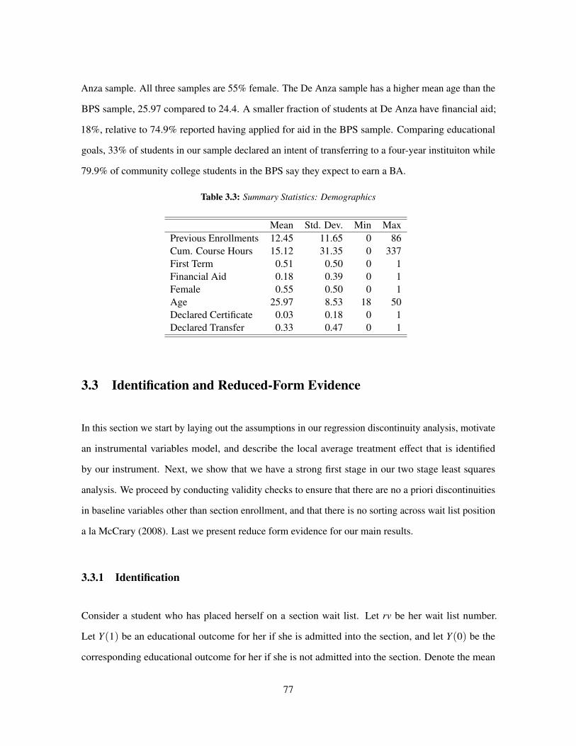
Anza sample. All three samples are 55% female. The De Anza sample has a higher mean age than the

BPS sample, 25.97 compared to 24.4. A smaller fraction of students at De Anza have financial aid;

18%, relative to 74.9% reported having applied for aid in the BPS sample. Comparing educational

goals, 33% of students in our sample declared an intent of transferring to a four-year instituiton while

79.9% of community college students in the BPS say they expect to earn a BA.

Table 3.3: Summary Statistics: Demographics

Mean Std. Dev. Min MaxPrevious Enrollments 12.45 11.65 0 86Cum. Course Hours 15.12 31.35 0 337First Term 0.51 0.50 0 1Financial Aid 0.18 0.39 0 1Female 0.55 0.50 0 1Age 25.97 8.53 18 50Declared Certificate 0.03 0.18 0 1Declared Transfer 0.33 0.47 0 1

3.3 Identification and Reduced-Form Evidence

In this section we start by laying out the assumptions in our regression discontinuity analysis, motivate

an instrumental variables model, and describe the local average treatment effect that is identified

by our instrument. Next, we show that we have a strong first stage in our two stage least squares

analysis. We proceed by conducting validity checks to ensure that there are no a priori discontinuities

in baseline variables other than section enrollment, and that there is no sorting across wait list position

a la McCrary (2008). Last we present reduce form evidence for our main results.

3.3.1 Identification

Consider a student who has placed herself on a section wait list. Let rv be her wait list number.

Let Y(1) be an educational outcome for her if she is admitted into the section, and let Y(0) be the

corresponding educational outcome for her if she is not admitted into the section. Denote the mean

77

outcome for students with wait list number rv had they all been admitted into their wait listed section

as E(Y(1)|RV = rv), similarly denote the mean outcome for students with wait-list number rv had

they not been admitted into their wait-listed section as E(Y(1)|RV = rv). Conditional on having wait

list number rv the effect of being admitted into the wait-listed section on the educational outcome is

E(Y(1) − Y(0)|RV = rv). Our identification strategy will allow us to measure the average effect for

students on the cusp of being admitted from the wait-list, for whom RV = 0. Denote this local average

treatment effect, LATE,

LAT E ≡ E(Y(1) − Y(0)|RV = 0). (3.1)

We measure this effect by estimating the four following quantities:

limrv↑0

E(X|RV = rv), limrv↓0

E(X|RV = rv) (3.2)

limrv↑0

E(Y |RV = rv), limrv↓0

E(Y |RV = rv), (3.3)

where X is an observed indicator for whether the student successfully enrolled in the wait-listed section

and Y is the observed educational outcome. By definition Y = Y(1) ⇐⇒ X = 1 so by conditional

expectation we can write E(Y |RV = rv) =

E(Y(1)|RV = rv)P(X = 1|RV = rv) + E(Y(0)|RV = rv)P(X = 0|RV = rv). (3.4)

Two necessary conditions are that there is a discontinuous jump in the likelihood of enrollment at the

threshold, i.e. limrv↑0 E(X|RV = rv) , limrv↓0 E(X|RV = rv). and that the functions E(Y( j)|RV) are

continuous at RV = 0 for j = 1, 0.

Define p j↑≡ limRV↑0 P(X = j|RV) and p j

↓≡ limRV↓0 P(X = j|RV) for j = 1, 0. E(Y( j)|RV)

continous at RV = 0 implies limRV↑0 E(Y( j)|RV) = limRV↓0 E(Y( j)|RV) = E(Y( j)|RV = 0) for

j = 1, 0.

∴ limRV↑0E(Y( j)|RV)P(X = j|RV) = E(Y( j)|RV = 0)p j

↑

78

and

limRV↓0E(Y( j)|RV)P(X = j|RV) = E(Y( j)|RV = 0)p j

↓

for j = 1, 0.

Now consider limRV↑0 E(Y |RV) − limRV↓0 E(Y |RV)

= E(Y(1)|RV = 0)p1↑+ E(Y(0)|RV = 0)p0

↑− E(Y(1)|RV = 0)p1

↓− E(Y(0)|RV = 0)p0

↓

= E(Y(1) − Y(0)|RV = 0) ∗ [p1↑− p1↓]

= LAT E ∗ [p1↑− p1↓]

In our regression discontinuity design we estimate the following system,

E(Y |RV , Z) = π10 + π1

1Z + g1(RV)

E(X|RV , Z) = π20 + π2

1Z + g2(RV)

where

π11 = LAT E ∗ [p1

↑− p1↓]

and

π21 = p1

↑− p1↓

We estimate the following instrumental variables model

E(Y |X, Z, W) = Xβ+ W′δ. (3.5)

E(X|Z, W) = Zπ12 + Wπ22. (3.6)

Here Z is an indicator for RV < 1, W contains continuous functions of the running variable and

demographic variables that are correlated with our set of outcomes, X is an indicator for whether

the student successfully enrolled in the wait-listed section, and Y is an outcome variable. The local

average treatment effect if denoted β. The exclusion restriction is that conditional on W and X the best

predictor of Y does not include Z.

79

What is the treatment and what is the local average treatment effect?

The treatment that we measure using the wait list discontinuity is the effect of admitting one additional

student into a section holding availability in all other sections fixed. In an ideal experiment that

estimates this same parameter only the supply one one section would be reduced. The response to

a treatment where a large fraction of sections are eliminated may be very different if reductions in

other courses and sections raises the expected costs substitution. A policy change that reduced overall

course offerings would decrease the chances of students enrolling in their most preferred sections as

well as the changes of enrolling in their second and third choices. The effects on student outcomes

of such a change are likely to be substantially different than the effects measured in this paper. In

the natural experiment that is the focus of this paper only the chances of enrollment in one section is

affected.

The local effect that we measure is for individuals who have placed themselves on the course wait-list

who are on the margin of being admitted into the section during the pre-registration period. It is

important to note that these students have placed themselves on wait lists where there is a substantial

chance of not being admitted into the section. In the next section we will see that around the threshold

the chances of not enrolling in the section are between ten and twenty percent. There may a substantial

portion of students who choose not to take this chance and who therefore do not place themselves on a

wait list. The effect of not enrolling in a section for these more averse students may be substantially

different than the effect that we measure in the population of student that place themselves on wait

lists.

3.3.2 First Stage

Enrollment into a section is not completely determined by whether or not a student was allowed to

enroll from the wait list. Therefore our estimation will be based on a fuzzy RD design. Making the

wait list cut-off produces a discontinuity in the probability of enrollment into the wait listed section

but it does not completely determine enrollment. Figure 3.1 shows a 13.4% increase in enrollment

80

associated with crossing the threshold from the right. Students on the right side of the red vertical line

in this figure remained on the wait list at the start of the term. The running variable tells us how other

students were ahead of them on the wait list ahead at the start of the term. Nonetheless, students that

remained on the wait list have a greater than 50% chance of enrolling in their desired section. This can

happen from enrolling in the section after the start of the term. On the left side of the figure we see

that a small fraction of students that were admitted into the section did not enroll, or enrolled and later

dropped the class.

Figure 3.1: First Stage: Mean Enrollment in Wait-listed Section as a Function of Relative Wait List Position

.5.6

.7.8

.91

Enro

llment R

ate

−20 −10 0 10 20waitlist position

Sample Size= 31328 and Jump = −.1348405786004608

Table 3.4 presents OLS regressions of the first stage equation. Each column presents results from a

local linear regression with a square kernel. The size of the bandwidth differs across the columns. The

first column uses a bandwidth of 20 on either side of the cut-off, the second column uses a bandwidth

of ten, and the third column uses a bandwidth of five. The coefficient on the instrument gives the

increase in probability of enrollment associated with crossing the threshold. We see that even with the

smallest bandwidth the coefficient remains at about ten percentage points.

81

Table 3.4: First Stage OLS Regressions

(1) (2) (3)Enrollment Enrollment Enrollment

Z 0.118*** 0.108*** 0.101***(0.00714) (0.00810) (0.0112)

RV -0.0113*** -0.0138*** -0.0129***(0.000521) (0.00113) (0.00343)

RVZ 0.00722*** 0.00965*** 0.00285(0.00194) (0.00220) (0.00509)

Constant 0.457*** 0.467*** 0.466***(0.00417) (0.00558) (0.00892)

Observations 51,802 41,940 27,365R-squared 0.038 0.028 0.020F 272.1 176.7 80.70

3.3.3 Validity Checks

We conduct two validity checks. First we check for discontinuities in baseline covariates at the

threshold, next we check whether there is bunching of the running variable at the threshold. Figures 3.2

and 3.3 plot of the average values of eight covariates conditional on wait list position. Figure 3.2

plots the fraction of each race and the fraction international students along the running variable. The

fraction white varies between 19 and 21.5%. The fraction Asian varies between 50 and 58%. While

this fraction is decreasing as a function of the running variable it does not change discontinuously at

the threshold. The fraction Hispanic varies between 8 and 12% and is steady around 11% as it crosses

the threshold. The fraction of international students stays between five and nine percent and while

there tends to be a higher fraction of international students on the left of the threshold this change is

continuous, Figure 3.3 examines mean age, fraction female, fraction of students with a high school

degree or less and the average number of credits earned in the sample. While the conditional mean age

varies smoothly with a general trend upward from 24 to 24.6 as the running variables goes from -5 to 5,

the fraction female varies downward from around .58 to .54 as the running variable goes from -5 to 5.

Previous educational attainment as measured by the fraction of students with a high school education

or less remains steady at around 70%. Cumulative course credits trend downward from an average

82

(a) White (b) Asian

(c) Hispanic (d) International

Figure 3.2: Smoothness on Covariates: Race and Citizenship Indicators

of 37 to an average of 30 at the threshold and further right. One should note that the discontinuity in

enrollment happens between 0 and 1 whereas the jump seem in panel d of Figure 3.3 occurs between

-1 and 0.

3.3.4 No Sorting Across Wait List Position

Whereas differences in observable characteristics between individuals on either side of the thresh-

old can be observed by examining the conditional distribution of each observable as it crosses the

threshold, a similar examination of unobservable characteristics cannot be done. However, we can

examine selection on unobservables due to sorting across the threshold (McCrary, 2008). Figure 3.4

is presented to examine differences in density across the threshold. Differences in density can arise

from manipulation of the running variable. It is rarely the case that individuals are indifferent between

83

(a) Age (b) Female

(c) HS or less (d) Credits

Figure 3.3: Smoothness on Covariates: Age, Gender, a priori Education

84

receiving treatment or not. In our case students would generally prefer to be enrolled in a selected

section rather not. If it were possible to manipulate the value of the running variable then there would

be incentives to move to lower wait list values. Movement of this type would have higher payoff the

closer a student is to crossing the threshold. We would then expect more of this movement to happen

for students with positive but small values of the running variable. Movements of this type move mass

from the positive side of the threshold to the negative side in the distribution of the running variable.

Figure 3.4 shows no evidence of this being the case.

Figure 3.4: No Sorting Across Wait-list position

0.0

5.1

.15

De

nsity

−10 −5 0 5 10Wait−List Position

3.3.5 Reduced Form Evidence

Before estimating our model more formally it will be helpful to examine the direct relationship between

relative wait list position and important outcomes. Figure 3.5 plots the mean number of courses in

which students successfully enrolled during the concurrent term, excluding the section that produced

85

the wait list position. The figure shows that moving a student below the threshold is associated with a

.126 increase in the number of other courses in which the student enrolled the concurrent term. Taken

together with a first stage estimate of between .10 and .12 this implies that successfully enrolling in an

additional course is associated with taking one fewer of the other courses available. Figure 3.6 shows

that a similar sized jump is present when moving over the threshold for the average number of other

sections in the same subject. By additivity this implies that the effect of enrolling in fewer classes

due to successfully enrolling in another is driven by substitution within classes in the same subject.

Figure 3.5: Enrollment in Other Sections, all subjects, concurrent term

11.2

1.4

1.6

1.8

(mean)

num

cours

es_cur

−20 −10 0 10 20dist_th2

Sample Size = 31328 and Jump = .1230923348838396

Enrolling in an undesirable section may have implications beyond a change in the number of courses

taken. Students may perform better when enrolled in a more desired class or when enrolled in the

same class at a more desired time. Figure3.7 plots the fraction of students who enrolled in school the

next term. This figure shows very little in the way of a jump at the point of discontinuity. This leads us

to conclude that enrollment in a more desired class does not effect enrollment in school the subsequent

term.

86

Figure 3.6: Enrollment in Other Sections in the same subject, concurrent term

−.5

0.5

1(m

ean)

num

cours

es_in

subj_

cur

−20 −10 0 10 20waitlist position

Sample Size = 31328 and Jump = .1265940544782833

3.4 IV Results

Now we turn to estimation of the effects of enrollment on various outcomes. First we examine the

effects on course enrollment within De Anza College. We will look at the number of enrolled courses

the concurrent quarter and the number of enrolled courses the next quarter. Next we turn to the effects

of enrollment on GPA and persistence. We will look at grade points averaged over all courses taken

the concurrent semester and the average grade point focusing on courses in the same subject. One

might think that enrolling in a more desirable section can lead to better preparation, more consistent

attendance, or other factors that would influence academic performance. Last we turn to enrollment

and attendance at other colleges. This analysis takes advantage of a match between our registration

files from De Anza College and data from the National Student Clearinghouse. Here we test whether

enrolling in a more desired course is associated with a higher probability of transferring to a four year

college. Alternatively we also test the hypothesis that failing to enroll in a desired course increases the

likelihood of seeking resources at another two-year college.

87

Figure 3.7: Stayed in School, 1 year

0.2

.4.6

.8(m

ean)

sta

yedin

school

−20 −10 0 10 20dist_th2

Sample Size = 31328 and Jump = −.0050495460143055

3.4.1 Course Enrollment

Tables 3.5 and 3.6 present our results for the effect on course enrollment within the same college.

Table 3.5 presents local linear two stage least square results using three alternative bandwidth choices.

Table 3.6 presents the same set of specifications using the optimal bandwidth selection and robust

standard estimation procedure of Cattaneo, Calonico, and Titiunik (2014) (CCT from here on). Our

main finding is that there is a robust and significant effect of successful enrollment on substitution away

from other courses in the same subject during the concurrent term. Panel A, columns one, two, and

three present TSLS estimates of this effect. From column one to column three we vary the bandwidth

of our local linear estimator from 20, to 10, to 5. We see that our measured coefficient on enrollment

increases as we narrow the bandwidth used for estimation. Panel A, column one of Table 3.6 uses

the CCT procedure to select optimal bandwidth for the regression. The point estimate given by the

procedure is squarely in the middle of the three corresponding estimates presented in Table 3.5. All

four estimates are lower than -1. In one case, column 3 panel A of Table 3.5 the estimate is significantly

88

Table 3.5: TSLS Estimates of Effects on Course Enrollment

Other Courses in Same Subject Total Courses in All Subjects(1) (2) (3) (4) (5) (6)

Panel A: Concurrent TermEnrolled -1.022*** -1.582*** -2.023*** 0.294* -0.00513 -0.391

(0.210) (0.237) (0.311) (0.179) (0.218) (0.329)RV -0.00479* -0.0214*** -0.0416*** -0.0215*** -0.0344*** -0.0546***

(0.00287) (0.00420) (0.00898) (0.00305) (0.00553) (0.0133)RVZ 0.0296*** 0.0448*** 0.0695*** 0.0347*** 0.0463*** 0.0582***

(0.00373) (0.00486) (0.0118) (0.00526) (0.00644) (0.0150)Constant 1.467*** 1.862*** 2.178*** 2.595*** 2.766*** 2.981***

(0.139) (0.159) (0.211) (0.0897) (0.114) (0.175)

R-squared 0.293 0.226 0.065 0.000 0.004Reduced Form p-val 0 0 0 0.0990 0.981 0.230

Panel B: Subsequent TermEnrolled -0.0149 -0.325 -0.230 0.129 0.240 0.560

(0.277) (0.374) (0.499) (0.297) (0.367) (0.538)RV 0.00113 -0.0117 -0.00161 -0.0125** -0.00945 0.00694

(0.00523) (0.0103) (0.0200) (0.00565) (0.00942) (0.0202)RVZ 0.0150* 0.0269** 0.0103 0.0158** 0.0130 0.00662

(0.00843) (0.0110) (0.0218) (0.00736) (0.00984) (0.0215)Constant 1.519*** 1.702*** 1.636*** 2.926*** 2.863*** 2.691***

(0.145) (0.204) (0.276) (0.150) (0.191) (0.284)

R-squared 0.000Reduced Form p-val 0.957 0.374 0.640 0.664 0.510 0.285Observations 51,429 41,631 27,193 51,429 41,631 27,193Bandwidth(spots) 20 10 5 20 10 5

*** p<0.01, ** p<0.05, * p<0.1

89

Table 3.6: TSLS Estimates of Effects on Course Enrollment (CCT)

Other Courses, Same Subject Total Courses, All Subjects(1) (2)

Panel A: Concurrent Term

RD_Estimate -1.545*** 0.123(0.334) (0.421)

Observations 15,156 21,688Panel B: Subsequent Term

RD_Estimate -0.270 1.113(1.069) (0.840)

Observations 4,462 12,108Standard errors in parentheses

*** p<0.01, ** p<0.05, * p<0.1

lower than -1. This might signal a quality/quantity trade-off in courses where students that fail to enroll

in a highly desired course substitute with more than one less desired course. Columns four, five and

six of panel A in Table 3.5 and column 2 of panel A of Table 3.6 present estimates of the effect of

successful enrollment on enrollment in all subjects the concurrent term. Here even though the point

estimates for one specification are significant at the 0.10 confidence level we do not see a consistent

significant effect on total enrollment.

Panel B of Table 3.5 and panel B of table 3.6 examine the effects of enrollment on course selection

the subsequent term. Columns one, two and three of panel B of table 3.5 and column 1 panel B of

Table 3.6 examine the effect on taking courses in the same subject the next term. The point estimates

in these regressions are each negative but none can rule out a coefficient of zero. Columns four, five

and six of panel B of Table 3.5 and column two of panel B of Table 3.6 measure the effect on the total

number of courses taken the subsequent school term. These regressions similarly show that there is

little indication of inter temporal substitution of courses across school terms.

90

Table 3.7: TSLS Estimates of Effects on GPA and Persistence (CCT)

(1) (2) (3)GPA GPA Enrolled

overall in subj. 1 yr latercur. term cur. term

RD_Estimate 0.150 0.0696 -0.174(0.366) (0.558) (0.199)

Observations 18,317 10,993 16,049Standard errors in parentheses

*** p<0.01, ** p<0.05, * p<0.1

3.4.2 GPA and Persistence

Next we turn to estimates of the effect of enrollment on GPA and persistence. Table 3.7 presents results

for three outcome measures. Column one examines the effect of successful enrollment on GPA for

the current term13. We see a positive but statistically insignificant coefficient. Column two turns to an

estimate of the effect on GPA for classes within the same subject. Again we see a slightly positive

but more noisy coefficient estimate. Column three of Table 3.7 presents our estimate of the effect of

course enrollment on an indicator for whether the student in seen in the same college one year later.

This regression measures a negative but insignificant effect of later school enrollment.

3.4.3 Enrollment at 4-year and other 2-year colleges

Last we examine enrollment and attendance at other institutions. We first examine short term outcomes,

where we look at where students are one year after the current term, then we look at longer term

outcomes where we examine whether we see students at another institution within three years. Column

one of Table 3.8 looks at the effect of enrolling in a college the next school term. Our estimate is that

an additional successful enrollment into a desired course is associated with a six percentage point

13For simplicity from here on in this section we only present results for the CCT estimation procedure, results usingalternative bandwidths are similar.

91

Table 3.8: TSLS Estimates of Effects on Four-Year College and Two-Year College Enrollment (CCT)

Enrollment at other Colleges(1) (2) (3) (4)4 yr other 2 yr 4 yr other 2 yr

nxt term nxt term nxt 3 yrs nxt 3 yrs

RD_Estimate 0.0612 0.112 0.150 -0.000126(0.0852) (0.0795) (0.156) (0.139)

Observations 16,049 16,049 16,049 16,049Standard errors in parentheses

*** p<0.01, ** p<0.05, * p<0.1

increase in the probability of attending a four year college the next term. However column two shows

that successful enrollment is a desired course is associated with an eleven percentage point increase in

the probability of attending a different two-year college. Neither of these estimate rule out no effect at

all of successful enrollment into a desired course. Columns three and four of Table 3.8 examine longer

term measures of these two outcome variables. Column three estimates that successfully enrolling in a

course is associated with a fifteen percentage point increase in the probability of attending a four year

school within three years. Column four gives a coefficient that indicates a negative effect of enrolling

in a different two year school that is one one hundredth of a percentage point. Neither estimates are

significantly different from zero. They are suggestive that the long term effect on four year college

enrollment may be positive.

3.5 Subgroup Analysis and Robustness Checks

This section examines the robustness of our findings and whether there are differential effects by sub-

group. The analysis looks at seven variables relating to course loads, gap, persistence and enrollment

at other colleges. We make measurements for eleven subgroups based on gender, race, age, citizenship,

and whether it is the student?s first term in college. We check the robustness of findings by varying

the number of control variables in the locally weighted regressions and by adding richer control

92

variables. Table C.1 presents our benchmark subgroup analysis. The regressions in this table estimate

the following model

E(Y |RV , W) = α+ δ′W + Z · β+3∑

j=1

γ0j RV j + γ1

j Z · RV j.

Table C.1 presents estimates of the regression discontinuity estimates using two stage least squares

and the method of bandwidth selection developed by CCT(2013a 2013b). The estimates use a third

order polynomial to approximate the underlying regression function, the expected outcome conditional

on the running variable as a function of the running variable. In the CCT algorithm that selects

bandwidth a fourth order polynomial is used to estimate bias due to functional form misspecification.

The bandwidth selected using this method is usually between two and three.

Here we look at eleven outcome variables for the overall population and for eleven subgroups. Each

entry in the table represents one estimate of the treatment effect for a separate two stage least squares

local regression.

It looks like there may be an effect on GPA for males, and an effect on GPA for non-first-time students.

There may be effect on whether you stayed in school 1yr for "young" students. There may be an effect

on whether you enrolled in a four year college on first time students and on non-foreign students.

There also seems to be an effect on whether you enrolled in another 2 year college on foreign students.

There may be an effect on whether first-time students enrolled in a four year college the next major

academic term. There may be an effect on whether foreign students enrolled in a two year college next

term.

E(Y |RV , W) = α+ δ′W + Z · β+3∑

j=1

γ0j RV j + γ1

j Z · RV j

The regressions in Table C.2 allow for linear functions of the running variable with different slopes on

either side of the threshold. They also control for cumulative course credits earned, cumulative number

of courses taken, whether the semester is the student’s first, whether the student received financial aid,

93

gender, and whether the student declared an intention to obtain a vocational certificate or transfer to

a four year college. Here we use a rectangular kernel with a bandwidth of five on either side of the

threshold.

E(Y |RV , W) = α+ δ′W + Z · β+ γ0RV + γ1Z · RV

The regressions in Table C.3 allow for linear functions of the running variable with different slopes on

either side of the threshold. As before they control for cumulative course credits earned, cumulative

number of courses taken, whether the semester is the student’s first, whether the student received

financial aid, gender, and whether the student declared an intention to obtain a vocational certificate or

transfer to a four year college. They also control for race fixed effects, registration priority group fixed

effects, term fixed effects and subject fixed effects. Here we use a rectangular kernel with a bandwidth

of five on either side of the threshold.

There is a positive effect of taking classes on enrollment in a 4 yr college, the effect exists even with

the addition of more extensive controls. It seems that it is driven by females and it is more pronounced

for non-foreign students and older students.

The coefficient in the first row in the column titled "enrolled in 4 yr college" is the two stage least

squares estimate of the effect of successfully enrolling in a wait listed section on whether the student

ever enrolls in a four year college. The estimated effect of 0.203 implies that missing a section

is causality associated with a 20 percentage point drop in the likelihood of attending a four year

college.

The first column has a coefficient of -1.34. This means that successfully enrolling in a desired section

is associated with taking 1.3 fewer courses in the same subject. Perfect substitution would a coefficient

of one and this estimate is not statistically significantly different than one. An estimate smaller than -1

would mean that each section not taken is replaced with more than one other course. This implies a

marginal rate of substitution greater than one and implies that wait listed courses are more useful than

the courses that replace them.

94

The regressions in C.4 allow for linear functions of the running variable with different slopes on either

side of the threshold. They also control for cumulative course credits earned, cumulative number of

courses taken, whether the semester is the student’s first, whether the student received financial aid,

gender, and whether the student declared an intention to obtain a vocational certificate or transfer to a

four year college. Here we use a rectangular kernel with a bandwidth of three on either side of the

threshold.

3.6 Conclusions

Course availability at two year colleges is a potentially important factor in the acquisition of human

capital. We examined the effect of course availability on later educational outcomes using a novel

administrative data set and a regression discontinuity design based on oversubscription to college

courses. We find a robust and substantial substitution effect. Specifically we find that successful

enrollment into a desired course section is causes students to take fewer courses in that subject the

concurrent term. We find some, but limited, evidence that students trade off quality for quantity when

they successfully enroll in desired courses. That is, successfully enrolling in a desired course causes

students to decrease the number of other courses in the same subject taken concurrently by more than

one. Future work may seek to explore these outcomes in other settings or with larger samples. Of

particular interest are the labor market outcomes of students who face course scarcity.

95

References

Abadie, A., Diamond, A. and Hainmueller, J. (2010). Synthetic control methods for comparative casestudies: Estimating the effect of california?s tobacco control program. Journal of the AmericanStatistical Association, 105 (490).

Aickin, M. (2001). Randomization, balance, and the validity and efficiency of design-adaptive alloca-tion methods. Journal of Statistical Planning and Inference, 94 (1), 97–119.

Akaike, H. (1974). A new look at the statistical model identification. Automatic Control, IEEETransactions on, 19 (6), 716–723.

Altham, P. M. (1971). The analysis of matched proportions. Biometrika, 58 (3), 561–576.

Altman, D. G. (1985). Comparability of randomised groups. The Statistician, pp. 125–136.

Anderson, T. W. and Rubin, H. (1949). Estimation of the parameters of a single equation in a completesystem of stochastic equations. The Annals of Mathematical Statistics, 20 (1), 46–63.

Andrabi, T., Das, J., Khwaja, A. I. and Zajonc, T. (2011). Do value-added estimates add value?accounting for learning dynamics. American Economic Journal: Applied Economics, 3 (3), 29–54.

Angrist, J. and Pischke, J.-S. (2010). The credibility revolution in empirical economics: How betterresearch design is taking the con out of econometrics. Tech. rep., National Bureau of EconomicResearch.

Angrist, J. D., Cohodes, S. R., Dynarski, S. M., Pathak, P. A. and Walters, C. R. (2013). Stand andDeliver: Effects of Boston’s Charter High Schools on College Preparation, Entry, and Choice. Tech.rep., National Bureau of Economic Research.

—, Imbens, G. W. and Rubin, D. B. (1996). Identification of causal effects using instrumental variables.Journal of the American statistical Association, 91 (434), 444–455.

— and Pischke, J.-S. (2008). Mostly harmless econometrics: An empiricist’s companion. Princetonuniversity press.

Arbia, G. (2006). Spatial econometrics: statistical foundations and applications to regional conver-gence. Springer.

96

Atkinson, A. C. (2002). The comparison of designs for sequential clinical trials with covariateinformation. Journal of the Royal Statistical Society: Series A (Statistics in Society), 165 (2),349–373.

Barrios, T., Diamond, R., Imbens, G. W. and Kolesar, M. (2012). Clustering, spatial correlations, andrandomization inference. Journal of the American Statistical Association, 107 (498), 578–591.

Bertrand, M., Duflo, E. and Mullainathan, S. (2004). How much should we trust differences-in-differences estimates? The Quarterly Journal of Economics, 119 (1), 249–275.

Beshears, J., Choi, J. J., Laibson, D., Madrian, B. C. and Milkman, K. L. (2011). The effect of providingpeer information on retirement savings decisions. Tech. rep., National Bureau of Economic Research.

Bester, C. A., Conley, T. G. and Hansen, C. B. (2011). Inference with dependent data using clustercovariance estimators. Journal of Econometrics, 165 (2), 137–151.

Birkett, N. J. (1985). Adaptive allocation in randomized controlled trials. Controlled clinical trials,6 (2), 146–155.

Bloom, N., Liang, J., Roberts, J. and Ying, Z. J. (2013). Does working from home work? Evidencefrom a Chinese experiment. Tech. rep., National Bureau of Economic Research.

Boswell, K. (2000). State funding for community colleges: A 50- state survey.

Bound, J., Lovenheim, M. F. and Turner, S. (2010). Why have college completion rates declined?an analysis of changing student preparation and collegiate resources. American economic journal.Applied economics, 2 (3), 129.

—, — and — (2012). Increasing time to baccalaureate degree in the united states. Education, 7 (4),375–424.

— and Turner, S. (2007). Cohort crowding: How resources affect collegiate attainment. Journal ofPublic Economics, 91 (5), 877–899.

Box, G. E., Hunter, J. S. and Hunter, W. G. (2005). Statistics for experimenters: design, innovation,and discovery, Hoboken. NJ: Wiley-Interscience.

Brockwell, P. J. and Davis, R. A. (2002). Introduction to time series and forecasting, vol. 1. Taylor &Francis.

Bruhn, M. and McKenzie, D. (2009). In pursuit of balance: Randomization in practice in developmentfield experiments. American economic journal: applied economics, pp. 200–232.

Calonico, S., Cattaneo, M. D. and Titiunik, R. (2013). Robust nonparametric confidence intervals forregression-discontinuity designs. Revision requested by Econometrica.

Card, D. and Lemieux, T. (2001). Can falling supply explain the rising return to college for youngermen? a cohort-based analysis. The Quarterly Journal of Economics, 116 (2), 705–746.

Casey, K., Glennerster, R. and Miguel, E. (2012). Reshaping institutions: Evidence on aid impactsusing a preanalysis plan*. The Quarterly Journal of Economics, 127 (4), 1755–1812.

97

Chaloner, K., Verdinelli, I. et al. (1995). Bayesian experimental design: A review. Statistical Science,10 (3), 273–304.

Chase, G. (1968). On the efficiency of matched pairs in bernoulli trials. Biometrika, 55 (2), 365–369.

Cochran, W. G. (1950). The comparison of percentages in matched samples. Biometrika.

Conley, T. G. (1999). Gmm estimation with cross sectional dependence. Journal of econometrics,92 (1), 1–45.

Cox, D. R. (1958). Two further applications of a model for binary regression. Biometrika, pp. 562–565.

— and Reid, N. (2000). The theory of the design of experiments. CRC Press.

DeMel, S., McKenzie, D. and Woodruff, C. (2008). Returns to capital in microenterprises: evidencefrom a field experiment. The Quarterly Journal of Economics, 123 (4), 1329–1372.

Deming, D. J., Goldin, C. and Katz, L. F. (2011). The For-Profit Postsecondary School Sector: NimbleCritters or Agile Predators? Tech. rep., National Bureau of Economic Research.

Diehr, P. (1995). Breaking the matches in a paired t-test for community interventions when the numberof pairs is small. Stat Med, 14 (13), 1491–1504.

Diggle, P., Heagerty, P., Liang, K.-Y. and Zeger, S. (2002). Analysis of longitudinal data. OxfordUniversity Press.

Donner, A. (1987). Statistical methodology for paired cluster designs. American Journal of Epidemiol-ogy, 126 (5), 972–979.

— and Klar, N. (2004). Pitfalls of and controversies in cluster randomization trials. American Journalof Public Health, 94 (3), 416.

Duflo, E., Glennerster, R. and Kremer, M. (2007). Using randomization in development economicsresearch: A toolkit. Handbook of development economics, 4, 3895–3962.

Efron, B. (1971). Forcing a sequential experiment to be balanced. Biometrika, 58 (3), 403–417.

Finkelstein, A., Taubman, S., Wright, B., Bernstein, M., Gruber, J., Newhouse, J. P., Allen, H.,Baicker, K. et al. (2012). The oregon health insurance experiment: Evidence from the first year*.The Quarterly Journal of Economics, 127 (3), 1057–1106.

Fisher, R. A. (1935). The design of experiments. Oliver & Boyd.

Flores-Lagunes, A., Gonzalez, A. and Neumann, T. (2010). Learning but not earning? the impact ofjob corps training on hispanic youth. Economic Inquiry, 48 (3), 651–667.

Fortin, N. M. (2006). Higher-education policies and the college wage premium: Cross-state evidencefrom the 1990s. The American Economic Review, pp. 959–987.

Gail, M. H., Mark, S. D., Carroll, R. J., Green, S. B. and Pee, D. (1996). On design considerationsand randomization-based inference for community intervention trials. Statistics in medicine, 15 (11),1069–1092.

98

Gill, A. M. and Leigh, D. E. (2003). Do the returns to community colleges differ between academicand vocational programs? Journal of Human Resources, 38 (1), 134–155.

Greenwald, B. C. (1983). A general analysis of bias in the estimated standard errors of least squarescoefficients. Journal of Econometrics, 22 (3), 323–338.

Greevy, R., Lu, B., Silber, J. H. and Rosenbaum, P. (2004). Optimal multivariate matching beforerandomization. Biostatistics, 5 (2), 263–275.

Greevy, R. A., Grijalva, C. G., Roumie, C. L., Beck, C., Hung, A. M., Murff, H. J., Liu, X. andGriffin, M. R. (2012). Reweighted mahalanobis distance matching for cluster-randomized trialswith missing data. Pharmacoepidemiology and drug safety, 21 (S2), 148–154.

Grubb, W. N. (1993). The varied economic returns to postsecondary education. Journal of HumanResources, 28 (2).

Hahn, J. (1998). On the role of the propensity score in efficient semiparametric estimation of averagetreatment effects. Econometrica, pp. 315–331.

—, Hirano, K. and Karlan, D. (2011). Adaptive experimental design using the propensity score.Journal of Business & Economic Statistics, 29 (1), 96–108.

Hansen, B. B. (2008). The prognostic analogue of the propensity score. Biometrika, 95 (2), 481–488.

Hansen, C. B. (2007). Generalized least squares inference in panel and multilevel models with serialcorrelation and fixed effects. Journal of Econometrics, 140 (2), 670–694.

Hastie, T., Tibshirani, R., Friedman, J. and Franklin, J. (2005). The elements of statistical learning:data mining, inference and prediction. The Mathematical Intelligencer, 27 (2), 83–85.

Heinemann, H. N. and Sussna, E. (1977). The economic benefits of a community college education.Industrial Relations: A Journal of Economy and Society, 16 (3), 345–354.

Hilmer, M. J. (1997). Does community college attendance provide a strategic path to a higher qualityeducation? Economics of Education Review, 16 (1), 59–68.

— (2000). Does the return to university quality differ for transfer students and direct attendees?Economics of Education Review, 19 (1), 47–61.

Hirano, K., Imbens, G. W. and Ridder, G. (2003). Efficient estimation of average treatment effectsusing the estimated propensity score. Econometrica, 71 (4), 1161–1189.

Hoxby, C. and Turner, S. (2013). Expanding college opportunities for high-achieving, low incomestudents. Stanford Institute for Economic Policy Research Discussion Paper, (12-014).

Ibragimov, R. and Muller, U. K. (2010). t-statistic based correlation and heterogeneity robust inference.Journal of Business & Economic Statistics, 28 (4), 453–468.

Imai, K. (2008). Variance identification and efficiency analysis in randomized experiments under thematched-pair design. Statistics in medicine, 27 (24), 4857–4873.

99

—, King, G., Nall, C. et al. (2009). The essential role of pair matching in cluster-randomizedexperiments, with application to the mexican universal health insurance evaluation. StatisticalScience, 24 (1), 29–53.

—, — and Stuart, E. A. (2008). Misunderstandings between experimentalists and observationalistsabout causal inference. Journal of the royal statistical society: series A (statistics in society), 171 (2),481–502.

Imbens, G. W. and Angrist, J. D. (1994). Identification and estimation of local average treatment effects.Econometrica: Journal of the Econometric Society, pp. 467–475.

—, King, G., McKenzie, D. and Ridder, G. (2009). On the finite sample benefits of stratification inrandomized experiments.

Jacobson, L., LaLonde, R. J. and Sullivan, D. (2005). The impact of community college retrainingon older displaced workers: Should we teach old dogs new tricks? Industrial and Labor RelationsReview, pp. 398–415.

Kane, T. J., McCaffrey, D. F., Miller, T. and Staiger, D. O. (2013). Have we identified effectiveteachers? validating measures of effective teaching using random assignment. research paper. metproject. Bill & Melinda Gates Foundation.

— and Rouse, C. E. (1995a). Comment on w. norton grubb:" the varied economic returns to post-secondary education: New evidence from the class of 1972". Journal of Human Resources, pp.205–221.

— and — (1995b). Labor-market returns to two-and four-year college. American Economic Review,85 (3), 600–614.

— and — (1999). The community college: Educating students at the margin between college andwork. The Journal of Economic Perspectives, pp. 63–84.

Karlan, D. (2013). Fighting poverty with actual evidence. Interview by Stephen Dubner.

Kasy, M. (2013). Why experimenters should not randomize, and what they should do instead. Tech.rep.

Leigh, D. E. and Gill, A. M. (1997). Labor market returns to community colleges: Evidence forreturning adults. Journal of Human Resources, pp. 334–353.

Lemieux, T. and Card, D. (2001). Education, earnings, and the ?canadian gi bill? Canadian Journal ofEconomics/Revue canadienne d’économique, 34 (2), 313–344.

Liang, K.-Y. and Zeger, S. L. (1986). Longitudinal data analysis using generalized linear models.Biometrika, 73 (1), 13–22.

Light, A. and Strayer, W. (2004). Who receives the college wage premium? assessing the labor marketreturns to degrees and college transfer patterns. Journal of Human Resources, 39 (3), 746–773.

Lock, K. and Rubin, D. (2012). Re-randomization to improve covariate balance in experiments. TheAnnals of Statistics, 40 (2), 1263–1282.

100

Lock, K. F. (2011). Re-randomization to Improve Covariate Balance in Randomized Experiments.Tech. rep.

Ludwig, J., Duncan, G. J., Gennetian, L. A., Katz, L. F., Kessler, R. C., Kling, J. R. and Sanbon-matsu, L. (2012). Neighborhood effects on the long-term well-being of low-income adults. Science,337 (6101), 1505–1510.

Lynn, H. and McCulloch, C. (1992). When does it pay to break the matches for analysis of a matched-pair design. Biometrics, 48, 397–409.

Manski, C. F., McFadden, D. et al. (1981). Structural analysis of discrete data with econometricapplications. MIT Press Cambridge, MA.

Mantel, N. (1967). The detection of disease clustering and a generalized regression approach. Cancerresearch, 27 (2 Part 1), 209–220.

Martin, D. C., Diehr, P., Perrin, E. B. and Koepsell, T. D. (1993). The effect of matching on thepower of randomized community intervention studies. Statistics in Medicine, 12 (3-4), 329–338.

McCrary, J. (2008). Manipulation of the running variable in the regression discontinuity design: Adensity test. Journal of Econometrics, 142 (2), 698–714.

McEntegart, D. J. (2003). The pursuit of balance using stratified and dynamic randomization tech-niques: an overview. Drug Information Journal, 37 (3), 293–308.

McKinlay, S. M. (1977). Pair-matching-a reappraisal of a popular technique. Biometrics, 33 (4),725–735.

McNemar, Q. (1947). Note on the sampling error of the difference between correlated proportions orpercentages. Psychometrika, 12 (2), 153–157.

Mosteller, F. (1952). Some statistical problems in measuring the subjective response to drugs.Biometrics, 8 (3), 220–226.

Moulton, B. R. (1986). Random group effects and the precision of regression estimates. Journal ofeconometrics, 32 (3), 385–397.

Neyman, J. (1934). On the two different aspects of the representative method: the method of stratifiedsampling and the method of purposive selection. Journal of the Royal Statistical Society, pp. 558–625.

Papadimitriou, C. H. and Steiglitz, K. (1998). Combinatorial optimization: algorithms and complexity.Courier Dover Publications.

Pearson, K. (1901). On lines and planes of closest fit to systems of points in space. PhilosophicalMagazine, 2 (11), 559–572.

Pocock, S. J. (1979). Allocation of patients to treatment in clinical trials. Biometrics, 35 (1), 183–197.

— and Simon, R. (1975). Sequential treatment assignment with balancing for prognostic factors in thecontrolled clinical trial. Biometrics, pp. 103–115.

101

Rosenbaum, P. R. (2002). Observational studies. Springer.

Rosenberger, W. F. and Sverdlov, O. (2008). Handling covariates in the design of clinical trials.Statistical Science, pp. 404–419.

Rouse, C. E. (1995). Democratization or diversion? the effect of community colleges on educationalattainment. Journal of Business & Economic Statistics, 13 (2), 217–224.

Rubin, D. B. (1973). Matching to remove bias in observational studies. Biometrics, pp. 159–183.

Ruggles, S., Sobek, M., Alexander, T., Fitch, C. A., Goeken, R., Hall, P. K., King, M. and Ronnander,C. (). Integrated public use microdata series: Version 4.0 [machine-readable database]. minneapolis,mn: Minnesota population center [producer and distributor], 2008. The Review of Economics andStatistics, 88 (2), 324–335.

Schabenberger, O. and Gotway, C. A. (2004). Statistical methods for spatial data analysis. CRC Press.

Schwarz, G. et al. (1978). Estimating the dimension of a model. The annals of statistics, 6 (2),461–464.

Scott, N. W., McPherson, G. C., Ramsay, C. R. and Campbell, M. K. (2002). The method of minimiza-tion for allocation to clinical trials: a review. Controlled clinical trials, 23 (6), 662–674.

Senn, S. (2004). Controversies concerning randomization and additivity in clinical trials. Statistics inMedicine, 23 (24), 3729–3753.

Shibata, R. (1976). Selection of the order of an autoregressive model by akaike’s information criterion.Biometrika, 63 (1), 117–126.

Shipley, M., Smith, P. and Dramaix, M. (1989). Calculation of power for matched pair studies whenrandomization is by group. International journal of epidemiology, 18 (2), 457–461.

Simon, R. (1979). Restricted randomization designs in clinical trials. Biometrics, 35 (2), 503.

Small, D. S., Ten Have, T. R. and Rosenbaum, P. R. (2008). Randomization inference in a group–randomized trial of treatments for depression: Covariate adjustment, noncompliance, and quantileeffects. Journal of the American Statistical Association, 103 (481), 271–279.

Snedecor, G. (). W and cochran, w g (1979) statistical methods.

Solomon, H. and Zacks, S. (1970). Optimal design of sampling from finite populations: A criticalreview and indication of new research areas. Journal of the American Statistical Association,65 (330), 653–677.

Spearman, C. (1904). “General intelligence,” objectively determined and measured. The AmericanJournal of Psychology, 15 (2), 201–292.

Splawa-Neyman, J., Dabrowska, D., Speed, T. et al. (1990). On the application of probability theory toagricultural experiments. essay on principles. section 9. Statistical Science, 5 (4), 465–472.

Stuart, A. (1957). The comparison of frequencies in matched samples. British Journal of StatisticalPsychology, 10 (1), 29–32.

102

Sukhatme, P. (1935). Contribution to the theory of the representative method. Supplement to theJournal of the Royal Statistical Society, pp. 253–268.

Tibshirani, R. (1996). Regression shrinkage and selection via the lasso. Journal of the Royal StatisticalSociety. Series B (Methodological), pp. 267–288.

Wei, L. (1978). The adaptive biased coin design for sequential experiments. The Annals of Statistics,pp. 92–100.

White, S. and Freedman, L. (1978). Allocation of patients to treatment groups in a controlled clinicalstudy. British Journal of Cancer, 37 (5), 849.

Wooldridge, J. M. (2010). Econometric analysis of cross section and panel data. MIT press.

103

Appendix A

Appendix to Chapter 1

A.1 Supplementary Results

For the general model, leaving aside terms that do not involve unknown parameters, the log likelihood

function is

L(γ|Y) = −12

ln (det(Ω(Z, γ))) −Y′Ω−1(Z, γ)Y/2.

The matrix Ω(Z, γ) is large in our illustrations, with dimension 2,590,190 by 2,590,190. Direct

maximization of the log likelihood function is therefore not feasible. However, because locations are

measured by puma locations, Ω(Z, γ) has a block structure, and calculations of the log likelihood

simplify and can be written in terms of first and second moments by puma. We first give a couple of

preliminary results.

Theorem 2. (Sylvester’s Determinant Theorem) Let A and B be arbitrary M × N matrices. Then:

det(IN + A′B) = det(IM + BA′).

Proof of Theorem 2: Consider a block matrix(

M1 M2M3 M4

). Then:

det(

M1 M2M3 M4

)= det

(M1 0M3 I

)det

(I M−1

1 M2

0 M4−M3 M−11 M2

)= det M1 det(M4 −M3M−1

1 M2)

104

similarly

det(

M1 M2M3 M4

)= det

(I M20 M4

)det

(M1−M2 M−1

4 M3 0M−1

4 M3 I

)= det M4 det(M1 −M2M−1

4 M3)

Letting M1 = IM, M2 = −B, M3 = A′, M4 = IN yields the result.

Lemma 5. (Determinant of Cluster CovarianceMatrix) Suppose C is an N ×M matrix of binary

cluster indicators, with C′C equal to a M ×M diagonal matrix, Σ is an arbitrary M ×M matrix, and

IN is the N-dimensional identity matrix. Then, for scalar σ2ε, and

Ω = σ2ε IN + CΣC′ ΩC = Σ + σ2

ε (C′C)−1,

we have

det(Ω) = (σ2ε )

N−M det(C′C) det(ΩC).

Proof of Lemma 5: By Sylvester’s theorem:

det(Ω) = (σ2ε )

N det(IN + CΣ/σ2εC′) = (σ2

ε )N det(IM + C′CΣ/σ2

ε )

= (σ2ε )

N det(IM + C′CΩC/σ2ε − IM) = (σ2

ε )N det(C′C) det(ΩC/σ2

ε )

= (σ2ε )

N−M(∏

Np)

det(ΩC).

Lemma 6. Suppose Assumptions 3 and 4 hold. Then for any N × N matrix Ω,

E [W′ΩW] =M1 · (M1 − 1)M · (M − 1)

· ι′NΩιN +M1 ·M0

M · (M − 1)· trace (C′ΩC) .

Proof of Lemma 6: We have

E[Wi ·W j] =

M1/M if ∀m, Cim = C jm,

(M1 · (M1 − 1))/(M · (M − 1)) otherwise.

it follows that

E[WW′] =M1 · (M1 − 1)M · (M − 1)

· ιN ι′N +

(M1

M−

M1 · (M1 − 1)M · (M − 1)

)·CC′

105

=M1 · (M1 − 1)M · (M − 1)

· ιN ι′N +

M1 ·M0

M · (M − 1)·CC′.

Thus

E[W′ΩW] = trace (E[ΩWW′])

= trace(Ω ·

(M1 · (M1 − 1)M · (M − 1)

· ιN ι′N +

M1 ·M0

M · (M − 1)·CC′

))=

M1 · (M1 − 1)M · (M − 1)

· ι′NΩιN +M1 ·M0

M · (M − 1)· trace (C′ΩC) .

Lemma 7. Suppose the N × N matrix Ω satisfies

Ω = σ2ε · IN + σ2

C ·CC′,

where IN is the N × N identity matrix, and C is an N ×M matrix of zeros and ones, with CιM = ιN

and C′ιN = (N/M)ιM, so that,

Ωi j =

σ2ε + σ2

C if i = j

σ2C if i , j,∀m, Cim = C jm,

0 otherwise,

(A.1)

Then, (i)

ln (det (Ω)) = N · ln(σ2ε

)+ M · ln

1 + NM·σ2

C

σ2ε

,

and, (ii)

Ω−1 = σ−2ε · IN −

σ2C

σ2ε · (σ

2ε + σ2

C · N/M)·CC′

Proof of Lemma 7: First, consider the first part. Apply Lemma 5 with

Σ = σ2C · IM, and C′C =

NM· IM, so that ΩC =

(σ2

C + σ2ε ·

MN

)· IM.

Then, by Lemma 5, we have

ln det(Ω) = (N −M) · ln(σ2ε) + M · ln(N/M) + ln det(ΩC)

= (N −M) · ln(σ2ε) + M · ln(N/M) + M · ln

(σ2

C + σ2ε ·

MN

)

106

= (N −M) · ln(σ2ε) + M · ln

( NMσ2

C + σ2ε

)= N · ln(σ2

ε) + M · ln1 + N

M·σ2

C

σ2ε

.

Next, consider part (ii). We need to show that

(σ2ε · IN + σ2

C ·CC′) σ−2

ε · IN −σ2

C

σ2ε · (σ

2ε + σ2

C · N/M)·CC′

= IN ,

which amounts to showing that

−σ2ε ·σ

2C

σ2ε · (σ

2ε + σ2

C · N/M)·CC′ + σ2

C ·CC′σ−2ε −CC′ ·

σ4C

σ2ε · (σ

2ε + σ2

C · N/M)·CC′ = 0.

This follows directly from the fact that C′C = (N/M) · IM and collecting the terms.

Proof of Lemma 2: By the constant treatment effect assumption, and by Assumption 2, the result

follows directly from the Neyman Lemma on unit-level randomization

Proof of Lemma 3: The unbiasedness result directly follows from the conditional unbiasedness

established in Lemma 2. Next we establish the second part of the Lemma. By the Law of Iterated

Expectations,

VU(Z) = V(E

[βols

∣∣∣ Y(0), Y(1), Z] ∣∣∣∣ Z, N1

)+ E

[V

(βols

∣∣∣ Y(0), Y(1), Z) ∣∣∣∣ Z, N1

]= E

[V

(βols

∣∣∣ Y(0), Y(1), Z) ∣∣∣∣ Z, N1

] (A.2)

where the second line follows since βols is unbiased. By Lemma 2, we have:

E[V

(βols

∣∣∣ Y(0), Y(1), Z) ∣∣∣∣ Z, N1

]= E

NN0 · N1 · (N − 2)

N∑i=1

(εi − ε)2

∣∣∣∣∣∣∣ Z, N1

Observe that we can write:

N∑i=1

(εi − ε)2 = (ε − ιN ι

′Nε/N)′(ε − ιN ι

′Nε/N)

= ε′ε − 2ε′ιN ι′Nε/N + ε′ιN ιN ιN ι′Nε/N2

= ε′ε − ε′ιN ι′Nε/N.

107

Hence:

VU(Z) =N

N0 · N1 · (N − 2)E

[ε′ε − ε′ιN ι

′Nε/N

∣∣∣ Z, N0, N1]

=N

N0 · N1 · (N − 2)trace

(E

[εε′ − ι′Nεε

′ιN/N∣∣∣ Z, N0, N1

])=

NN0 · N1 · (N − 2)

(trace (Ω(Z)) − ι′NΩ(Z)ιN/N)

which establishes (1.11). Finally, we prove the third part of the Lemma. By Lemma 1, βols is unbiased

conditional on Z, W, so that by argument like in Equation (A.2) above, we can also write:

VU(Z) = V(E

[βols

∣∣∣ Z, W] ∣∣∣∣ Z, N1

)+ E

[V

(βols

∣∣∣ Z, W) ∣∣∣∣ Z, N1

]= E

[V

(βols

∣∣∣ Y(0), Y(1), Z) ∣∣∣∣ Z, N1

]which equals E [VR (Y(0), Y(1), Z)

∣∣∣ Z, N1] by (A.2).

Proof of Lemma 4: To show the first part of the Lemma, observe that under constant cluster size,

βols =

∑Mm=1(Ym −

¯Y)2(Wm −¯W)∑

m(Wm −¯W)2

where Ym = (N/M)−1 ∑i : Cim=1 Yi, and ¯Y = M−1 ∑

m Ym = Y , and ¯W = W. Therefore, we can apply

Lemma 2, treating cluster averages (Ym, Wm, εm) as a unit of observation, which yields the result.

To show the second part, again by Lemma 2, βols is unbiased, so that by the Law of Iterated Expectations,

and the first part of the Lemma,

VU(Z) = V(E

[βols

∣∣∣ Y(0), Y(1), Z] ∣∣∣∣ Z, M1

)+ E

[V

(βols

∣∣∣ Y(0), Y(1), Z) ∣∣∣∣ Z, M1

]= E

[V

(βols

∣∣∣ Y(0), Y(1), Z) ∣∣∣∣ Z, M1

]= E

M(M − 2) ·M0 ·M1

M∑m=1

(εm − ε

)2∣∣∣∣∣∣∣ Z, M1

Hence, it suffices to show that

E

M∑s=1

(εs − ε

)2∣∣∣∣∣∣∣ Z, M1

= (M2

N2 · trace (C′Ω(Z)C) −MN2 ι

′Ω(Z)ι)

.

Note that in general CιM = ιN , and under Assumption 4, it follows that C′C = (N/M) · IM. We can

108

write

εm = (C′C)−1 C′ε =MN

C′ε, and ε =1Mι′M (C′C)−1 C′ε =

1Nι′Nε,

so thatM∑

m=1

(εm − ε

)2=

(MN

C′ε −1MιMι′Nε

)′ ( MN

C′ε −1MιMι′Nε

)

=

((MN

C′ −1NιMι′N

)ε

)′ (( MN

C′ −1NιMι′N

)ε

).

= ε′(

MN

C −1NιN ι′M

)′ ( MN

C′ −1NιMι′N

)ε.

Thus

E

M∑m=1

(εs − ε

)2∣∣∣∣∣∣∣ Z, M1

= E

[ε′

(MN

C −1NιN ι′M

)′ ( MN

C′ −1NιMι′N

)ε

∣∣∣∣∣∣ Z, M1

]

= trace(E

[(MN

C −1NιN ι′M

)′ ( MN

C′ −1NιMι′N

)εε′

∣∣∣∣∣∣ Z, M1

])= trace

((MN

C −1NιN ι′M

)′ ( MN

C′ −1NιMι′N

)Ω(Z)

)= trace

((MN

C′ −1NιMι′N

)Ω(Z)

(MN

C −1NιN ι′M

)′)=

M2

N2 · trace (C′Ω(Z)C) −MN2 · ι

′NΩ(Z)ιN .

Proof of Theorem 1: Under Assumption 4, W = M1/M, which is non-random. Hence, in order to

prove VU(Ω(Z), Z) = VU(Ω(Z, γ), Z), it suffices to show that trace(C′Ω(Z)C) = trace(C′Ω(Z, (σε, σ2S ))C).

The log likelihood function based on the specification (A.1) is

L(σ2ε,σ

2S |Y, Z) = −

12· ln

(Ω

(Z,σ2

ε,σ2S

))−

12·Y′Ω(σ2

ε,σ2S )−1Y.

The expected value of the log likelihood function is

E[L(σ2

ε,σ2S |Y, Z)

∣∣∣ Z]= −

12

ln(Ω

(Z,σ2

ε,σ2S

))−

12·E

[Y′Ω(Z,σ2

ε,σ2C)−1Y

]= −

12· ln

(Ω

(Z,σ2

ε,σ2S

))−

12· trace

(E

[Ω

(Z,σ2

ε,σ2S

)−1YY′

)]

109

= −12· ln

(Ω

(Z,σ2

ε,σ2S

))−

12· trace

(Ω

(Z,σ2

ε,σ2S

)−1Ω(Z)

).

Using Lemma 7, this is equal to

E[L(σ2

ε,σ2S |Y, Z)

∣∣∣ Z]= −

N2· ln(σ2

ε) −M2· ln

(1 + N/M ·σ2

S /σ2ε

)−

12 ·σ2

ε

· trace(Ω(Z)) +σ2

S

2 ·σ2ε · (σ

2ε + σ2

S · N/M)· trace (C′Ω(Z)C) .

The first derivative of the expected log likelihood function with respect to σ2S is

∂

∂σ2S

E[L(σ2

ε,σ2S |Y, Z)

∣∣∣ Z]= −

N2 · (σ2

ε + N/M ·σ2S )

+trace (C′Ω(Z)C)

(σ2ε + σ2

S · (N/M))2

Hence the first order condition for σ2S implies that

trace (C′Ω(Z)C) = N · (σ2ε + σ2

S · (N/M)).

For the misspecified error-covariance matrix Ω(Z, γ) we have

trace (C′Ω(Z, γ)C) =M∑

m=1

(N2

m · σ2S + Nm · σ

2ε

).

By equality of the cluster sizes this simplifies to

trace (C′Ω(Z, γ)C) = N ·(σ2ε + σ2

S · (N/M))= trace (C′Ω(Z)C) .

110

Appendix B

Appendix to Chapter 2

B.1 Supplementary Results

Given a matched pairs randomization one may wish to estimate an average treatment effect and/or test

the null of no effect using t-statistic based tests. On the one hand, one can view the data as a set of N

outcome measurements from the experimental units where N/2 have been treated. Given the paired

nature of the data proper standard errors can be computed by regressing the N outcome measurements

on a treatment indicator alongside a set of N/2 pair indicators.

On the other hand, one can view the data as a set of n = N/2 within pair differences, where one is

simply estimating the mean of the differences. Proper standard errors here can be computed using the

sample standard deviation of the differences.

In fact, tests using the mean of within-pair differences, and regressions of the pooled experimental

units with pair dummies both accounting for and not accounting for heteroskedasticity in standard

ways, are equivalent. We show this below.

The first of two complimentary results is that these two procedures are mathematically equivalent. They

produce the same estimates of the treatment effect and the same standard errors. One may note that

111

standard errors in the first case will depend on whether or not the experimenter makes an assumption

about homoskedasticy. The second complimentary result we present is that in the first procedure

standard errors constructed under the homoskedasticy assumption and standard errors constructed

using the Huber-Eicker-White procedure are equivalent.

This second result holds more generally for all stratifications with equal sized strata and equal numbers

of treated and control units within each stratum, for example when experimental units are blocked into

groups of four and in each block two units are treated.

The mean of the differences

Let d1, ..., dn be the set of within pair differences where the untreated unit is subtracted from

the treated unit in each pair. Let b ≡ 1n∑n

i=1 di be the treatment effect estimator.

Further let us test the the null of no treatment effect with a two tailed test using the test statistic.

There is a finite sample justification for this test that comes from an assumption of i.i.d normal

errors,

tstat1 ≡b√

1n

1n−1

∑ni=1(di − b)2

(B.1)

and compare it to the critical values from a t-distribution with n − 1 degrees of freedom. Indi-

vidual units with pair dummies and regression

Let Y be an N × 1 vector of outcomes of experimental units where we denote the ith element of

this vector yi for i = 1, ..., N. Also let X be an N × k matrix, where k = N/2 + 1, the first column

of X is a treatment indicator and the next N columns of X are pair indicators.

Without loss of generality let the rows of Y and X that correspond to the same pair be grouped

together such that the odd numbered rows correspond to treated observations.

Now consider the projection of Y onto the column space of X. It is a standard result that least

112

squares with group indicators is equivalent to within group least squares and with two observa-

tions per group, this is the same as least squares on the difference which here is the mean of di.

The coefficient on the treatment indicator in the least squares fit is 2N

∑Ni=1(−1)i+1yi =

1n∑

di =

b. The coefficient on the first pair dummy is 12 (y1 − b + y2), the coefficient on the second pair

dummy is 12 (y3 − b+ y4) and in general the coefficient for the ith pair dummy is 1

2 (y2i−1 − b+ y2i).

The formulas for these coefficients can be verified by checking that the implied residuals are in

fact orthogonal to the columns of X. Let the residual for the ith be ei for i = 1, ..., N.

Denote Huber-Eicker-White heteroskedasticity consistent covariance estimator as

ΣW ≡N

N − k(X′X)−1

N∑i=1

xix′ie2i

(X′X)−1 (B.2)

where xi is the ith row of X.

One would test the null of no treatment effect using the test statistic

tstat2 ≡b√

ΣW1,1

(B.3)

where ΣW1,1 is the (1, 1) element of ΣW .

Assuming homoskedasticity the standard covariance estimator is

ΣH ≡ (X′X)−1 1N − k

N∑i=1

e2i (B.4)

One would test the null of no treatment effect using the test statistic

tstat3 ≡b√

ΣH1,1

(B.5)

where ΣH1,1 is the (1, 1) element of ΣH .

In each case following the linear regression model one would use critical values from a t-distribution

with N − k = N − N2 − 1 = n − 1 degrees of freedom.

113

Claim 1: ΣW1,1 = ΣH1,1

proof:

Let Is be the identity matrix of size s, let k = N2 + 1, and let 1s,t be a matrix of size s × t where

each element is a one. First notice that X =(1k−1,1 ⊗ (

10), Ik−1 ⊗ (

11)

)so

X′X =

(11,k−11k−1,1) ⊗ ((1, 0)(10)) (11,k−1Ik−1) ⊗ ((1, 0)(1

1))

(Ik−11k−1,1) ⊗ ((1, 1)(10)) (Ik−1Ik−1) ⊗ ((1, 1)(1

1))

=

k − 1 11,k−1

1k−1,1 2Ik−1

,

and that the inverse of this block matrix is

(X′X)−1 =2N

2 −11,k−1

−1k−1,1N4 Ik−1 + 1k−1,k−1

. (B.6)

So ΣH1,1 = 4N

1N−k

∑Ni=1 e2

i .

Now we show that ΣW1,1 = 4N

1N−k

∑Ni=1 e2

i .

Consider

ΣW ≡N

N − k(X′X)−1

N∑i=1

xix′ie2i

(X′X)−1 =N

N − k(X′X)−1X′ΩX(X′X)−1 (B.7)

where xi is the ith row of X, and Ω is N × N where Ωi, j = e2i 1i = j.

114

Next note that (X′X)−1X′Ω =

1N

2e21 −2e2

2 2e23 −2e2

4 . . . 2e2N−1 −2e2

N

(N2 − 1)e2

1 (N2 + 1)e2

2 −e23 e2

4 . . . −e2N−1 e2

N

−e21 e2

2 (N2 − 1)e2

3 (N2 + 1)e2

4 . . . −e2N−1 e2

N

−e21 e2

2 −e23 e2

4 . . . −e2N−1 e2

N...

......

......

...

−e21 e2

2 −e23 e2

4 . . . (N2 − 1)e2

N−1 (N2 + 1)e2

N

and X(X′X)−1 =

1N

2 N2 − 1 −1 −1 −1 . . . −1

−2 N2 + 1 1 1 1 . . . 1

2 −1 N2 − 1 −1 −1 . . . −1

−2 1 N2 + 1 1 1 . . . 1

2 −1 −1 N2 − 1 −1 . . . −1

−2 1 1 N2 + 1 1 . . . 1

......

......

... . . ....

2 −1 −1 −1 −1 . . . N2 − 1

−2 1 1 1 1 . . . N2 + 1

.

So the (1,1) element of (X′X)−1X′ΩX(X′X)−1 is 4N2

∑Ni=1 e2

i . Thus ΣW1,1 = NN−k

4N2

∑Ni=1 e2

i .

Claim 2: ΣH1,1 = 1n

1n−1

∑ni=1(di − b)2

proof:

115

Consider the residuals from the regression:

e1 = y1 −12(y1 − b + y2) − b

e2 = y2 −12(y1 − b + y2)

e3 = y3 −12(y3 − b + y4) − b

e4 = y4 −12(y3 − b + y4)

...

and in general note that we can change indexes as follows

N∑i=1

e2i =

n∑k=1

(e22i−1 + e2

2i) (B.8)

=n∑

k=1

(y2k−1 −12(y2k−1 − b + y2k) − b)2 + (y2k −

12(y2k−1 − b + y2k))

2

=14

n∑k=1

(dk − b)2 + (b − dk)2 =

12

∑(dk − b)2.

So

ΣH1,1 =2

N(N − k)

n∑k=1

(dk − b)2

=1

n(N − (N2 + 1))

n∑k=1

(dk − b)2

=1

n(n − 1)

n∑k=1

(dk − b)2

Generalization of claim 1 The result that regressions of the pooled experimental units with pair

dummies both accounting for and not accounting for heteroskedasticity in standard ways are

equivalent can be generalized to randomizations with equal sized strata and equal numbers of

treated and control units within each stratum. Suppose that we have equal sized strata, let S

116

denote their size, S even, S divides N, and denote the number of strata ns ≡NS . Now X has the

form

X =

[1 N

2 ,1 ⊗

(10

); Ins ⊗ 1S ,1

]and

X′X =

N2

S2 11,ns

S2 1ns,1 S Ins

so

(X′X)−1 =

4N − 2

N 11,ns

− 2N 1ns,1 ·

where we omit the lower right block of the inverse and note that it is not necessary for the

remainder of the proof. Note that Ω is diagonal with (k, k) element e2k , [(X′X)−1]k,1 = 4/N if

k = 1 and −2/N if k > 1 , (3) X j,1 = 1 if j odd and 0 else, and each sub-vector X j,2:K has one 1

and K-1 zeros for all j, so that the conditions of lemma 1 hold. By lemma 1

[(X′X)−1X′ΩX(X′X)−1]1,1 =4

N2

N∑i=i

e2i

Lemma 1 If

• (A1) Ω is diagonal with (k, k) element e2k , k = 1, ..., N

• (A2)

[(X′X)−1]k,1 =

4/N, if k = 1

−2/N, if k > 1,

• (A3.1)

X j,1 =

1, if j odd

0, else,

• and (A3.2) X j,2:K has one 1 and K-1 zeros,

then [(X′X)−1X′ΩX(X′X)−1]1,1 = 4N2

∑Ni=1 e2

i

117

proof:

[(X′X)−1X′ΩX(X′X)−1]1,1 =N∑

k=1

[(X′X)−1X′]1,kΩk,k[X(X′X)−1]k,1

=∑N

k=1 Ωk,k[X(X′X)−1]2k,1. By lemma 2 |[X(X′X)−1]k,1| =2N for all k. So

[(X′X)−1X′ΩX(X′X)−1]1,1 =N∑

k=1

e2k

4N2 .

Lemma 2 If conditions (A2) and (A3) of lemma 1 hold, then

[X(X′X)−1]k,1 =

2N , if k is odd

− 2N , if k is even.

(B.9)

proof: By definition [X(X′X)−1] j,1 =∑N

k=1 X j,k[(X′X)−1]k,1 . First consider

K∑k=2

X j,k[(X′X)−1]k,1.

Since k > 1, [(X′X)−1]k,1 = −2/N by condition (A2), and X j,2:K has one 1 and K-1 zeros by

condition (A3.2). So∑N

k=2 X j,k[(X′X)−1]k,1 = 2N . Now if j is odd then X1,1 = 1 by condition (A3)

and [(X′X)−1]1,1 = 4/N by condition (A2), so [X(X′X)−1]k,1 = 4−2N . If j is even then X1,1 = 0 by

condition (A3) and∑N

k=1 X j,k[(X′X)−1]k,1 =∑N

k=2 X j,k[(X′X)−1]k,1 = 2N .

Proofs

We are given E(θi|X, ε) = θ.

and that Ti is independent of Yi(0), Yi(1), Xi.

Yi(0) = θi + r(Xi) + εi

Yi = Tiθi + r(Xi) + εi

Dk = T2k−1[Y2k−1(1) − Y2k(0)] + (1 − T2k−1)[Y2k(1) − Y2k−1(0)]

= T2k−1[θ2k−1 + r(X2k−1) − r(X2k) + ε2k−1 − ε2k]

+ (1 − T2k−1)[θ2k + r(X2k) − r(X2k−1) + ε2k − ε2k−1]

118

Since E(εi|T ) = 0, then

E(Dk|T , X, θ) = T2k−1[θ2k−1 + r(X2k−1) − r(X2k)]

+ (1 − T2k−1)[θ2k + r(X2k) − r(X2k−1)]

= θ2k + T2k−1[θ2k−1 − θ2k] + (2T2k−1 − 1)[r(X2k−1) − r(X2k)] (B.10)

By iterated expectations

E(Dk|X, θ) = E(E(Dk|T , X, θ)|X, θ)

= θ2k +12(θ2k−1 − θ2k)

=12(θ2k−1 + θ2k)

By iterated expectations again, E(θi|X, ε) = θ =⇒ E(θi|X) = θ, and

E(Dk|X) = E(E(Dk|X, θ)|X)

=12

E(θ2k−1 + θ2k|X)

= θ (B.11)

Note that

cov(θi, εi|X) = E(θiεi|X) − E(θi|X)E(εi|X)

= E(θiεi|X) since E(εi|X) = 0

= E(E(θiεi|X, ε)|X)

= E(εiE(θi|X, ε)|X)

= E(εiE(θi)|X) by A1

= E(θi)E(εi|X)

= 0 since E(εi|X) = 0

119

Now consider

var(Dk|T .X) = T2k−1[var(θ2k−1|T , X) + var(ε2k−1|T , X) + var(ε2k|T , X)]

+ (1 − T2k−1)[var(θ2k|T , X) + var(ε2k−1|T , X) + var(ε2k|T , X)]

Since T is independent of X and θ we need not condition on it.

= T2k−1var(θ2k−1|X) + (1 − T2k−1)var(θ2k|X) + var(ε2k−1|X) + var(ε2k|X) (B.12)

Now we obtain the variance conditional just on X from

var(Dk|X) = E(var(Dk|T , X)|X) + var(E(Dk|T , X)|X) (B.13)

The first term in B.13 comes from taking the expectation of B.12 over the distribution of T2k−1.

This gives

E(var(Dk|T , X)|X) =12[var(θ2k−1|X) + var(θ2k|X)] + var(ε2k−1|X) + var(ε2k|X) (B.14)

The second term in B.13 comes from taking the conditional expectation of B.10 holding T , X

fixed and then taking the variance of the result.

E(Dk|T , X) = θ+ (2T2k−1 − 1)[r(X2k−1) − r(X2k)]

var(E(Dk|T , X)|X) = [r(X2k−1) − r(X2k)]2

since var(2T2k−1 − 1) = 1. So combining B.14 and B.13 gives

var(Dk|X) =12[var(θ2k−1|X) + var(θ2k|X)]

+ var(ε2k−1|X) + var(ε2k|X)

+ [r(X2k−1) − r(X2k)]2

Furthermore,

cov(Dk, Dh|X) = 0

120

since given X, Dk is a function of ((θ2k−1, θ2k, ε2k−1, ε2k, T2k−1), and Dh is a function of

((θ2h−1, θ2h, ε2h−1, ε2h, T2h−1), and these stochastic terms are independent.

B.2 Supplementary Tables

Table B.1: Mean Squared Error for Multiple Randomization Methods 1

Ntrainingsample = 100, Nexperiment = 100 Randomization MethodCR MPY0 MPYRidge MPYLAS S O MPYAIC MPYBIC MPYorcl

Labor income (Mexico) 1.000 1.026 0.767 0.764 0.748 0.753 0.752Microenterprise profits (Sri Lanka) 1.000 0.960 0.864 0.861 0.870 0.892 0.869Math test score (Pakistan) 1.000 1.006 0.614 0.585 0.588 0.588 0.601Height z-score (Pakistan) 1.000 0.987 0.650 0.681 0.677 0.666 0.679Household expenditures (Indonesia) 1.000 0.953 0.738 0.738 0.772 0.772 0.737Child schooling (Indonesia) 1.000 1.010 0.848 0.891 0.899 0.877 0.871

Notes: This table gives mean squared error estimates relative to complete randomization. CR is complete randomization,that is, under no stratification. MPY0 is matching on the lagged value of the outcome in each dataset. The next four columnsMPYx match pairs according to the predicted outcome, where the prediction is formed from a training dataset using methodx. Ridge uses ridge regression (Tibshirani 1996) where the penalty term is chosen to minimize the mean squared errorunder ten-fold cross validation. LAS S O uses the least absolute shrinkage and selection operator (Tibshirani,1996) where thepenalty term is chosen to minimize the mean squared error under ten-fold cross validation. AIC uses the model among the27 sub-models that has the lowest value of the Akaike information criterion (Akaike, 1974). BIC uses the model among the27 sub-models that has the lowest value of the Bayes information criterion (Schwarz, 1978). In each of the four methods thefull model is linear in a constant and the seven “balancing variables” and corresponds to the data generating process. Thesize of the the training sample used to estimate these predictors is Ntrainingsample = 100 and the total number of unit in eachsimulated experiment is Nexperiment = 100.

Table B.2: Size control for Multiple Randomization Methods 1

Ntrainingsample = 100, Nexperiment = 100 Randomization MethodCR MPY0 MPYRidge MPYLAS S O MPYAIC MPYBIC MPYorcl

Labor income (Mexico) 0.050 0.051 0.050 0.051 0.048 0.051 0.047Microenterprise profits (Sri Lanka) 0.054 0.051 0.051 0.049 0.049 0.049 0.047Math test score (Pakistan) 0.051 0.051 0.050 0.048 0.051 0.051 0.047Height z-score (Pakistan) 0.052 0.049 0.048 0.052 0.052 0.052 0.054Household expenditures (Indonesia) 0.051 0.046 0.049 0.048 0.050 0.052 0.048Child schooling (Indonesia) 0.049 0.051 0.049 0.053 0.050 0.046 0.052

Notes: This table gives the rejection rates for .95 significance tests using multiple randomization methods. The randomiza-tions methods and sample sizes are described in Table 2.5.

121

Table B.3: Power for Multiple Randomization Methods 1

Ntrainingsample = 100, Nexperiment = 100 Randomization MethodTE CR MPY0 MPYRidge MPYLAS S O MPYAIC MPYBIC MPYorcl

Labor income (Mexico) 0.19 0.147 0.143 0.190 0.182 0.177 0.181 0.177Microenterprise profits (Sri Lanka) 0.12 0.097 0.087 0.093 0.094 0.090 0.097 0.097Math test score (Pakistan) 0.23 0.203 0.195 0.288 0.292 0.304 0.299 0.290Height z-score (Pakistan) 0.26 0.242 0.248 0.332 0.342 0.334 0.333 0.326Household expenditures (Indonesia) 0.52 0.726 0.726 0.831 0.827 0.818 0.815 0.832Child schooling (Indonesia) 0.24 0.218 0.212 0.240 0.237 0.231 0.229 0.239

Notes: This table gives the rejection rates for .95 significance tests, under the treatment effect given under column T E, using multiplerandomization methods. The treatment effects are presented as standard deviations of the outcome variable. The randomizationsmethods and sample sizes are described in Table 2.5.

Table B.4: Mean Squared Error for Multiple Randomization Methods 2

Ntrainingsample = 2000, Nexperiment = 30 Randomization MethodCR MPY0 MPYRidge MPYLAS S O MPYAIC MPYBIC MPYorcl

Labor income (Mexico) 1.000 1.001 0.796 0.768 0.776 0.806 0.773Microenterprise profits (Sri Lanka) 1.000 0.966 0.885 0.877 0.884 0.865 0.853Math test score (Pakistan) 1.000 0.997 0.594 0.583 0.577 0.595 0.577Height z-score (Pakistan) 1.000 0.971 0.640 0.648 0.659 0.679 0.643Household expenditures (Indonesia) 1.000 1.056 0.752 0.742 0.826 0.802 0.749Child schooling (Indonesia) 1.000 0.961 0.826 0.834 0.846 0.839 0.842

Notes: This table gives mean squared error estimates relative to complete randomization. CR is complete randomization,that is, under no stratification. MPY0 is matching on the lagged value of the outcome in each dataset. The next four columnsMPYx match pairs according to the predicted outcome, where the prediction is formed from a training dataset using methodx. Ridge uses ridge regression (Tibshirani 1996) where the penalty term is chosen to minimize the mean squared errorunder ten-fold cross validation. LAS S O uses the least absolute shrinkage and selection operator (Tibshirani,1996) where thepenalty term is chosen to minimize the mean squared error under ten-fold cross validation. AIC uses the model among the27 sub-models that has the lowest value of the Akaike information criterion (Akaike 1974). BIC uses the model among the27 sub-models that has the lowest value of the Bayes information criterion (Schwarz 1978). In each of the four methods thefull model is linear in a constant and the seven “balancing variables” and corresponds to the data generating process. Thesize of the the training sample used to estimate these predictors is Ntrainingsample = 2000 and the total number of unit in eachsimulated experiment is Nexperiment = 100.

Table B.5: Size control for Multiple Randomization Methods 2

Ntrainingsample = 2000, Nexperiment = 30 Randomization MethodCR MPY0 MPYRidge MPYLAS S O MPYAIC MPYBIC MPYorcl

Labor income (Mexico) 0.048 0.049 0.054 0.051 0.050 0.049 0.050Microenterprise profits (Sri Lanka) 0.050 0.050 0.053 0.052 0.051 0.047 0.048Math test score (Pakistan) 0.052 0.053 0.049 0.049 0.047 0.052 0.051Height z-score (Pakistan) 0.052 0.050 0.047 0.051 0.051 0.050 0.050Household expenditures (Indonesia) 0.047 0.055 0.048 0.045 0.052 0.051 0.049Child schooling (Indonesia) 0.052 0.050 0.048 0.050 0.050 0.050 0.051

Notes: This table gives the rejection rates for .95 significance tests using multiple randomization methods. The randomiza-tions methods and sample sizes are described in Table 2.5.

122

Table B.6: Power for Multiple Randomization Methods 2

Ntrainingsample = 2000, Nexperiment = 30 Randomization MethodTE CR MPY0 MPYRidge MPYLAS S O MPYAIC MPYBIC MPYorcl

Labor income (Mexico) 0.18 0.077 0.074 0.085 0.088 0.082 0.084 0.085Microenterprise profits (Sri Lanka) 0.12 0.066 0.060 0.063 0.060 0.063 0.059 0.060Math test score (Pakistan) 0.23 0.096 0.094 0.110 0.118 0.113 0.121 0.121Height z-score (Pakistan) 0.26 0.110 0.102 0.124 0.127 0.127 0.130 0.122Household expenditures (Indonesia) 0.51 0.269 0.263 0.340 0.334 0.317 0.318 0.328Child schooling (Indonesia) 0.24 0.101 0.091 0.102 0.104 0.104 0.105 0.101

Notes: This table gives the rejection rates for .95 significance tests, under the treatment effect given under column T E, using multiplerandomization methods. The treatment effects are presented as standard deviations of the outcome variable. The randomizationsmethods and sample sizes are described in Table 2.5.

Table B.7: Mean Squared Error for Multiple Randomization Methods 3

Ntrainingsample = 2000, Nexperiment = 300 Randomization MethodCR MPY0 MPYRidge MPYLAS S O MPYAIC MPYBIC MPYorcl

Labor income (Mexico) 1.000 0.963 0.717 0.705 0.713 0.714 0.702Microenterprise profits (Sri Lanka) 1.000 0.989 0.902 0.879 0.865 0.913 0.873Math test score (Pakistan) 1.000 1.019 0.604 0.574 0.591 0.583 0.574Height z-score (Pakistan) 1.000 1.008 0.674 0.655 0.667 0.666 0.661Household expenditures (Indonesia) 1.000 0.984 0.718 0.737 0.753 0.779 0.733Child schooling (Indonesia) 1.000 0.983 0.835 0.856 0.867 0.848 0.846

Notes: This table gives mean squared error estimates relative to complete randomization. CR is complete randomization, thatis, under no stratification. MPY0 is matching on the lagged value of the outcome in each dataset. The next four columnsMPYx match pairs according to the predicted outcome, where the prediction is formed from a training dataset using methodx. Ridge uses ridge regression (Tibshirani 1996) where the penalty term is chosen to minimize the mean squared errorunder ten-fold cross validation. LAS S O uses the least absolute shrinkage and selection operator (Tibshirani,1996) where thepenalty term is chosen to minimize the mean squared error under ten-fold cross validation. AIC uses the model among the 27

sub-models that has the lowest value of the Akaike information criterion (Akaike 1974). BIC uses the model among the 27

sub-models that has the lowest value of the Bayes information criterion (Schwarz 1978). In each of the four methods the fullmodel is linear in a constant and the seven “balancing variables” and corresponds to the data generating process. The sizeof the the training sample used to estimate these predictors is Ntrainingsample and the total number of unit in each simulatedexperiment is Nexperiment.

Table B.8: Size control for Multiple Randomization Methods 3

Ntrainingsample = 2000, Nexperiment = 300 Randomization MethodCR MPY0 MPYRidge MPYLAS S O MPYAIC MPYBIC MPYorcl

Labor income (Mexico) 0.054 0.048 0.050 0.052 0.052 0.049 0.049Microenterprise profits (Sri Lanka) 0.052 0.050 0.055 0.050 0.045 0.053 0.049Math test score (Pakistan) 0.049 0.052 0.050 0.049 0.050 0.048 0.048Height z-score (Pakistan) 0.049 0.049 0.053 0.049 0.051 0.049 0.051Household expenditures (Indonesia) 0.052 0.049 0.051 0.054 0.047 0.052 0.049Child schooling (Indonesia) 0.049 0.046 0.051 0.052 0.053 0.051 0.052

Notes: This table gives the rejection rates for .95 significance tests using multiple randomization methods. The randomizationsmethods and sample sizes are described in Table 2.5.

123

Table B.9: Power for Multiple Randomization Methods 3

Ntrainingsample = 2000, Nexperiment = 300 Randomization MethodTE CR MPY0 MPYRidge MPYLAS S O MPYAIC MPYBIC MPYorcl

Labor income (Mexico) 0.18 0.359 0.361 0.464 0.473 0.465 0.464 0.464Microenterprise profits (Sri Lanka) 0.12 0.180 0.173 0.191 0.196 0.198 0.199 0.193Math test score (Pakistan) 0.24 0.492 0.503 0.706 0.736 0.722 0.718 0.730Height z-score (Pakistan) 0.27 0.611 0.600 0.787 0.784 0.776 0.771 0.790Household expenditures (Indonesia) 0.51 0.993 0.994 0.999 0.999 0.999 0.998 0.999Child schooling (Indonesia) 0.24 0.531 0.541 0.608 0.614 0.602 0.608 0.610

Notes: This table gives the rejection rates for .95 significance tests, under the treatment effect given under column T E, using multiplerandomization methods. The treatment effects are presented as standard deviations of the outcome variable. The randomizationsmethods and sample sizes are described in Table 2.5.

124

Appendix C

Appendix to Chapter 3

C.1 Supplementary Tables

125

Table C.1: Cubic Local Polynomial Results, (CCT)

Number of Enrolled Courses ex-post GPA Enrolled in Collegeallcoursesin subj

othercourses

in samesubj

allcourses

overall in subj stayedinschool1yr

in 4-yrcollege

in other2-yrcollege

in 4-yrcollege

in other2-yrcollege

in Current Term Next Term w/ in 3 yrs Next Termoverall -

1.769***0.071 3.558 -0.0550 -0.306 -0.0486 -0.107 0.0805 0.0305 -0.0448 -0.0319

s.e. (0.397) (0.377) (18.99) (0.439) (0.246) (0.894) (0.136) (0.119) (0.0948) (0.0681) (0.0504)Obs. 23,138 34,004 9,298 23,132 22,033 17,507 34,127 34,127 34,127 34,127 34,127Males -

1.180***0.635 1.025 -0.101 -

0.769**0.383 0.151 -0.0974 -0.0312 -0.0485 -0.0477

s.e. (0.454) (0.417) (1.492) (0.482) (0.389) (1.239) (0.154) (0.135) (0.106) (0.0774) (0.0572)Obs. 11,321 16,632 4,670 11,391 14,919 8,557 16,682 16,682 16,682 16,682 16,682Females -

2.429***-0.931 1.582 0.0796 -0.280 -0.574 -0.525* 0.417 0.156 -0.0239 0.000487

s.e. (0.803) (0.842) (1.598) (0.913) (0.691) (1.366) (0.303) (0.258) (0.192) (0.132) (0.0983)Obs. 11,763 17,300 4,599 11,688 15,280 8,911 17,373 17,373 17,373 17,373 17,373Non-First Time -

1.620***0.232 1.725 -0.207 -

0.587**-0.573 -0.0530 -0.0229 0.0665 -0.108 -0.0604

s.e. (0.621) (0.419) (4.716) (0.476) (0.292) (1.897) (0.151) (0.136) (0.105) (0.0808) (0.0560)Obs. 18,956 27,591 7,676 18,722 17,835 14,640 27,692 27,692 27,692 27,692 27,692Fist-Time -

1.926***-0.573 0.406 0.725 0.652 0.372 -0.324 0.526* -0.141 0.231* 0.0814

s.e. (0.446) (0.899) (6.470) (1.243) (0.741) (0.642) (0.321) (0.292) (0.230) (0.140) (0.122)Obs. 4,182 6,413 1,844 4,410 5,674 2,867 6,435 6,435 6,435 6,435 6,435Non-foreign -

1.690***0.0269 0.0757 0.0726 -0.236 1.188 -0.0819 -0.156 0.198* -0.0547 0.0195

s.e. (0.399) (0.406) (1.737) (0.466) (0.373) (1.286) (0.150) (0.455) (0.114) (0.0747) (0.0595)Obs. 15,986 23,910 5,804 15,688 21,017 11,941 24,008 34,042 24,008 24,008 24,008Foreign -1.885** 0.156 0.719 -0.355 -1.593* -2.308 -0.185 -0.102 -

0.463**-0.0170 -0.183*

s.e. (0.870) (0.860) (0.619) (1.065) (0.920) (1.881) (0.298) (0.262) (0.233) (0.154) (0.106)Obs. 7,152 10,094 2,874 7,444 9,248 5,566 10,119 10,119 10,119 10,119 10,119Minority 4.483 0.0434 -1.274 0.849 -1.028 -0.401 -0.524 1.234 0.0781 0.188 -0.0459s.e. (6.973) (1.990) (2.903) (1.306) (2.376) (1.142) (0.761) (0.960) (0.638) (0.267) (0.278)Obs. 3,874 5,821 1,537 3,664 4,913 3,223 5,847 5,847 7,134 5,847 5,847Asian -

1.118***0.397 0.635 -0.220 -0.619 -0.434 -0.100 -0.164 0.0278 -0.0570 -0.0231

s.e. (0.367) (0.514) (1.364) (0.614) (0.431) (0.776) (0.187) (0.175) (0.131) (0.0987) (0.0662)Obs. 11,497 16,678 5,145 12,125 15,188 8,838 16,721 16,721 16,721 16,721 16,721White -

1.637***-0.825 -0.0257 -0.246 -0.603 0.953 -0.101 0.162 -0.391 -0.0798 0.0297

s.e. (0.559) (0.630) (1.505) (0.631) (0.662) (1.147) (0.687) (0.193) (0.541) (0.118) (0.0805)Obs. 4,884 7,108 2,241 4,555 6,339 3,842 8,696 7,139 8,696 7,139 7,139Old -3.722 0.619 1.002 -0.292 -0.818 7.654 0.267 0.325 -0.0371 -0.170 -0.0207s.e. (3.731) (0.885) (1.501) (0.966) (0.659) (30.53) (0.292) (0.255) (0.192) (0.159) (0.107)Obs. 7,920 11,481 3,963 6,680 9,782 7,414 11,544 11,544 11,544 11,544 11,544Young -

1.475***-0.191 1.140 0.0154 -0.413 0.155 -0.260* -0.0193 0.0509 0.00273 -0.0361

s.e. (0.306) (0.397) (2.455) (0.479) (0.402) (0.795) (0.156) (0.136) (0.109) (0.0742) (0.0565)Obs. 15,218 22,523 7,138 16,452 20,483 11,501 22,583 22,583 22,583 22,583 22,583

This table presents estimates of the regression discontinuity estimates using two stage least squares and the method of bandwidth selectiondeveloped by CCT(2013a 2013b). The estimates use a third order polynomial to approximate the underlying regression function, theexpected outcome conditional on the running variable as a function of the running variable. In the CCT algorithm that selects bandwidth afourth order polynomial is used to estimate bias due to functional form misspecification. The bandwidth selected using this method isusually between two and three.

126

Table C.2: Local Linear TSLS, with control variables (BW of 5)

Number of Enrolled Courses ex-post GPA Enrolled in Collegeallcoursesin subj

othercourses

in samesubj

allcourses

overall in subj stayedinschool1yr

in 4-yrcollege

in other2-yrcollege

in 4-yrcollege

in other2-yrcollege

in Current Term Next Term w/ in 3 yrs Next Termoverall -

1.943***0.138 0.0864 0.448 -0.0662 0.422 -0.0828 0.273** 0.0780 0.0576 0.00205

s.e. (0.470) (0.338) (0.441) (0.435) (0.329) (0.831) (0.110) (0.122) (0.0941) (0.0683) (0.0496)Obs. 27,403 40,442 8,930 27,363 36,058 20,881 40,593 40,593 40,593 40,593 40,593Males -

1.852***0.0719 -0.694 0.596 -0.292 0.0525 -0.0955 0.0658 0.0322 0.0171 -0.0483

s.e. (0.564) (0.416) (0.720) (0.557) (0.420) (1.026) (0.140) (0.149) (0.120) (0.0863) (0.0653)Obs. 13,375 19,719 4,461 13,420 17,685 10,156 19,781 19,781 19,781 19,781 19,781Females -2.044** 0.327 0.877 0.368 0.215 0.729 -0.0525 0.520** 0.137 0.0975 0.0616s.e. (0.798) (0.568) (0.736) (0.695) (0.541) (1.407) (0.177) (0.220) (0.154) (0.112) (0.0797)Obs. 14,028 20,723 4,469 13,943 18,373 10,725 20,812 20,812 20,812 20,812 20,812Non-First Time Students -1.653 0.482 0.280 0.463 -0.329 0.989 -0.105 0.287* 0.0824 0.0189 -0.0284s.e. (1.043) (0.432) (0.614) (0.535) (0.419) (1.974) (0.143) (0.158) (0.117) (0.0905) (0.0616)Obs. 22,326 32,611 7,301 21,991 29,122 17,339 32,733 32,733 32,733 32,733 32,733Fist-Time Students -

2.079***-0.679 -0.305 0.466 0.629 0.197 0.000616 0.229 0.0635 0.140* 0.0677

s.e. (0.377) (0.542) (0.608) (0.717) (0.536) (0.589) (0.142) (0.172) (0.154) (0.0831) (0.0851)Obs. 5,077 7,831 1,629 5,372 6,936 3,542 7,860 7,860 7,860 7,860 7,860Non-foreign Students -

2.164***-0.0154 -0.391 0.275 0.0409 1.592 -0.119 0.353** 0.152 0.0402 0.0365

s.e. (0.544) (0.408) (0.856) (0.502) (0.394) (1.142) (0.138) (0.156) (0.124) (0.0839) (0.0658)Obs. 18,945 28,486 5,585 18,586 25,080 14,225 28,607 28,607 28,607 28,607 28,607Foreign Students -1.696* 0.350 0.292 0.686 -0.399 -2.524 -0.0551 0.0911 -0.0601 0.0916 -0.0587s.e. (0.931) (0.606) (0.501) (0.849) (0.595) (2.193) (0.179) (0.196) (0.142) (0.118) (0.0716)Obs. 8,458 11,956 3,345 8,777 10,978 6,656 11,986 11,986 11,986 11,986 11,986Minority Students -

1.706***0.812*** 0.155 -0.698* 0.158 -0.549 -0.175* 0.0662 0.0609 -0.0145 -

0.00835s.e. (0.661) (0.305) (0.281) (0.424) (0.303) (2.686) (0.0982) (0.0845) (0.0835) (0.0458) (0.0497)Obs. 7,173 11,569 2,147 7,105 9,782 5,166 11,639 11,639 11,639 11,639 11,639Asian Students -1.227** 0.140 0.258 0.563 0.282 0.325 -0.0830 -0.0231 0.100 0.0435 0.0723s.e. (0.555) (0.538) (0.943) (0.722) (0.498) (0.967) (0.172) (0.193) (0.149) (0.112) (0.0765)Obs. 13,683 19,982 4,934 14,407 18,182 10,587 20,031 20,031 20,031 20,031 20,031White Students -

1.554***-0.0181 0.534 0.829 -0.596 0.404 -

0.370**0.303* 0.151 -0.0121 0.0609

s.e. (0.527) (0.497) (0.548) (0.533) (0.503) (0.935) (0.182) (0.184) (0.142) (0.105) (0.0759)Obs. 5,729 8,343 1,658 5,336 7,454 4,513 8,377 8,377 8,377 8,377 8,377Old Students -4.058 0.284 0.445 0.0430 -0.277 3.184 0.485* 0.651** -0.0210 0.0641 -0.0641s.e. (7.204) (0.772) (0.647) (0.948) (0.673) (13.49) (0.288) (0.309) (0.195) (0.159) (0.106)Obs. 9,360 13,606 2,954 7,995 11,658 7,126 13,682 13,682 13,682 13,682 13,682Young Students -

1.849***0.126 -0.591 0.609 0.108 0.418 -

0.245**0.170 0.0997 0.0589 0.0211

s.e. (0.363) (0.360) (0.648) (0.484) (0.372) (0.720) (0.120) (0.133) (0.107) (0.0723) (0.0561)Obs. 18,043 26,836 5,976 19,368 24,400 13,755 26,911 26,911 26,911 26,911 26,911Cum. Course credits × × × × × × × × × × ×

Cum. Enrolled courses × × × × × × × × × × ×

First Time Status × × × × × × × × × × ×

Received Fin. Aid × × × × × × × × × × ×

Female × × × × × × × × × × ×

Goal Voc. Cert. × × × × × × × × × × ×

Goal 4-yr Degree × × × × × × × × × × ×

These regressions allow for linear functions of the running variable with different slopes on either side of the threshold. They also control forcumulative course credits earned, cumulative number of courses taken, whether the semester is the student’s first, whether the student receivedfinancial aid, gender, and whether the student declared an intention to obtain a vocational certificate or transfer to a four year college. Here we use arectangular kernel with a bandwidth of five on either side of the threshold.

E(Y |RV , W) = α+ δ′W + Z · β+ γ0RV + γ1Z · RV

127

Table C.3: Local Linear TSLS, with more extensive control variables (BW of 5)

Number of Enrolled Courses ex-post GPA Enrolled in Collegeallcoursesin subj

othercourses

in samesubj

allcourses

overall in subj stayedinschool1yr

in 4-yrcollege

in other2-yrcollege

in 4-yrcollege

in other2-yrcollege

in Current Term Next Term w/ in 3 yrs Next Termoverall -

1.340***0.261 0.242 0.436 -0.0656 0.565 -0.0897 0.203* 0.0357 0.0662 -0.0117

s.e. (0.337) (0.343) (0.342) (0.449) (0.344) (0.825) (0.101) (0.122) (0.0966) (0.0703) (0.0514)Obs. 27,398 40,431 8,929 27,355 36,047 20,876 40,582 40,582 40,582 40,582 40,582Males -

1.327***0.174 0.0253 0.703 -0.292 0.235 -0.0213 -0.0358 -0.0235 0.00410 -0.0738

s.e. (0.484) (0.444) (0.487) (0.601) (0.470) (1.203) (0.133) (0.159) (0.129) (0.0930) (0.0715)Obs. 13,373 19,714 4,460 13,416 17,680 10,154 19,776 19,776 19,776 19,776 19,776Females -

1.293***0.436 0.457 0.207 0.233 0.550 -0.148 0.460** 0.117 0.143 0.0545

s.e. (0.474) (0.542) (0.491) (0.691) (0.523) (1.123) (0.156) (0.205) (0.150) (0.111) (0.0777)Obs. 14,025 20,717 4,469 13,939 18,367 10,722 20,806 20,806 20,806 20,806 20,806Non-First Time Students -0.583 0.552 0.530 0.450 -0.376 0.791 -0.0803 0.200 0.0279 0.0376 -0.0402s.e. (0.645) (0.435) (0.493) (0.541) (0.440) (1.483) (0.130) (0.155) (0.119) (0.0923) (0.0633)Obs. 22,321 32,600 7,300 21,983 29,111 17,334 32,722 32,722 32,722 32,722 32,722Fist-Time Students -

1.915***-0.238 -0.442 0.379 0.835 0.765 -0.0929 0.184 0.0426 0.113 0.0730

s.e. (0.345) (0.506) (0.442) (0.767) (0.562) (0.745) (0.127) (0.169) (0.156) (0.0815) (0.0861)Obs. 5,077 7,831 1,629 5,372 6,936 3,542 7,860 7,860 7,860 7,860 7,860Non-foreign Students -

1.389***0.0774 0.525 0.210 0.0483 1.679 -0.129 0.284* 0.0977 0.0457 0.0198

s.e. (0.359) (0.412) (0.686) (0.522) (0.417) (1.093) (0.126) (0.154) (0.125) (0.0857) (0.0674)Obs. 18,942 28,478 5,584 18,581 25,072 14,222 28,599 28,599 28,599 28,599 28,599Foreign Students -1.360* 0.460 0.0781 0.899 -0.493 -2.600 -0.0439 0.0311 -0.0688 0.0930 -0.0572s.e. (0.731) (0.627) (0.423) (0.933) (0.605) (2.083) (0.167) (0.203) (0.150) (0.124) (0.0754)Obs. 8,456 11,953 3,345 8,774 10,975 6,654 11,983 11,983 11,983 11,983 11,983Minority Students -

1.373***0.636** 0.0452 -0.511 0.189 -

0.00798-0.0999 0.0550 0.0178 -

0.00944-0.0167

s.e. (0.323) (0.271) (0.229) (0.363) (0.273) (1.067) (0.0805) (0.0778) (0.0765) (0.0422) (0.0461)Obs. 7,172 11,566 2,147 7,103 9,780 5,165 11,636 11,636 11,636 11,636 11,636Asian Students -1.030** 0.167 0.162 0.618 0.312 0.447 -0.113 -0.122 0.0803 0.0806 0.0710s.e. (0.433) (0.582) (0.619) (0.852) (0.557) (0.999) (0.164) (0.211) (0.163) (0.123) (0.0838)Obs. 13,680 19,975 4,933 14,401 18,175 10,584 20,024 20,024 20,024 20,024 20,024White Students -

1.341***0.0994 0.631 0.740 -0.675 0.156 -

0.373**0.258 0.0803 -0.0291 0.0398

s.e. (0.446) (0.481) (0.475) (0.518) (0.521) (0.853) (0.163) (0.176) (0.137) (0.103) (0.0738)Obs. 5,728 8,341 1,658 5,336 7,452 4,512 8,375 8,375 8,375 8,375 8,375Old Students -0.426 0.636 0.414 0.124 -0.219 1.508 0.356 0.592** -0.0725 0.0657 -0.0819s.e. (1.174) (0.731) (0.484) (0.910) (0.688) (2.508) (0.235) (0.279) (0.186) (0.151) (0.102)Obs. 9,359 13,603 2,954 7,993 11,655 7,125 13,679 13,679 13,679 13,679 13,679Young Students -

1.601***0.146 0.0849 0.537 0.117 0.642 -

0.238**0.0933 0.0637 0.0854 0.00949

s.e. (0.324) (0.372) (0.460) (0.509) (0.390) (0.873) (0.112) (0.137) (0.112) (0.0763) (0.0590)Obs. 18,039 26,828 5,975 19,362 24,392 13,751 26,903 26,903 26,903 26,903 26,903Race FEs × × × × × × × × × × ×

Reg. Priority Group FEs × × × × × × × × × × ×

Year × Term FEs × × × × × × × × × × ×

Subj. FEs × × × × × × × × × × ×

These regressions allow for linear functions of the running variable with different slopes on either side of the threshold. As before they control forcumulative course credits earned, cumulative number of courses taken, whether the semester is the student’s first, whether the student receivedfinancial aid, gender, and whether the student declared an intention to obtain a vocational certificate or transfer to a four year college. They alsocontrol for race fixed effects, registration priority group fixed effects, term fixed effects and subject fixed effects. Here we use a rectangular kernelwith a bandwidth of five on either side of the threshold.

128

Table C.4: Local Linear TSLS, with more extensive control variables (BW of 3)

Number of Enrolled Courses ex-post GPA Enrolled in Collegeallcoursesin subj

othercourses

in samesubj

allcourses

overall in subj stayedinschool1yr

in 4-yrcollege

in other2-yrcollege

in 4-yrcollege

in other2-yrcollege

in Current Term Next Term w/ in 3 yrs Next Termoverall -1.469** 0.283 2.648 0.460 -1.111 -0.0263 -0.193 0.392 -0.0437 0.0861 -0.0961s.e. (0.579) (0.726) (8.075) (0.843) (0.787) (1.257) (0.217) (0.271) (0.201) (0.146) (0.110)Obs. 18,046 26,276 5,840 17,897 23,375 13,530 26,372 26,372 26,372 26,372 26,372Males -1.067* 0.685 -27.74 0.359 -1.357 -0.547 0.0224 -0.0248 -0.101 0.0259 -0.0768s.e. (0.645) (0.745) (1,026) (0.789) (0.894) (1.812) (0.217) (0.259) (0.212) (0.151) (0.116)Obs. 8,840 12,850 2,955 8,773 11,520 6,613 12,891 12,891 12,891 12,891 12,891Females -2.048 -0.780 8.599 0.731 -0.847 0.414 -0.781 1.431 0.166 0.235 -0.144s.e. (1.437) (2.078) (36.20) (2.879) (1.760) (2.071) (0.773) (1.199) (0.522) (0.398) (0.286)Obs. 9,206 13,426 2,885 9,124 11,855 6,917 13,481 13,481 13,481 13,481 13,481Non-First Time Students -1.321 0.643 -42.70 0.146 -1.995 0.0493 -0.0767 0.229 -0.0932 0.0493 -0.188s.e. (1.187) (0.948) (1,261) (1.065) (1.407) (3.439) (0.278) (0.333) (0.255) (0.195) (0.150)Obs. 14,650 21,127 4,738 14,352 18,831 11,225 21,205 21,205 21,205 21,205 21,205Fist-Time Students -

1.585***-0.316 -2.381 0.929 0.385 0.528 -0.452 0.719 0.0373 0.155 0.134

s.e. (0.520) (1.065) (5.395) (1.387) (0.889) (0.908) (0.319) (0.460) (0.319) (0.175) (0.181)Obs. 3,396 5,149 1,102 3,545 4,544 2,305 5,167 5,167 5,167 5,167 5,167Non-foreign Students -1.526** 0.167 0.184 0.0895 -0.578 1.338 -0.226 0.598 0.231 0.0542 -

0.00124s.e. (0.619) (0.866) (1.027) (0.993) (0.883) (1.527) (0.271) (0.366) (0.268) (0.176) (0.139)Obs. 12,429 18,378 3,615 12,072 16,139 9,174 18,453 18,453 18,453 18,453 18,453Foreign Students -1.598 0.182 1.107 1.675 -2.536 -4.523 -0.110 -0.0872 -0.617 0.135 -0.274s.e. (1.353) (1.400) (1.091) (2.052) (2.102) (5.185) (0.378) (0.455) (0.455) (0.278) (0.215)Obs. 5,617 7,898 2,225 5,825 7,236 4,356 7,919 7,919 7,919 7,919 7,919Minority Students -

1.296***0.679** -0.0293 -0.569 0.227 -0.0645 -0.0822 0.0770 0.0146 -0.0222 -0.0334

s.e. (0.332) (0.279) (0.236) (0.392) (0.283) (1.096) (0.0828) (0.0800) (0.0786) (0.0435) (0.0480)Obs. 6,820 11,013 2,047 6,768 9,300 4,915 11,080 11,080 11,080 11,080 11,080Asian Students -0.621 0.174 1.078 0.403 -0.527 0.130 -0.390 0.164 -0.0877 0.225 -0.130s.e. (0.554) (0.923) (1.260) (1.168) (0.783) (1.133) (0.295) (0.341) (0.258) (0.211) (0.136)Obs. 8,996 12,926 3,205 9,422 11,755 6,841 12,965 12,965 12,965 12,965 12,965White Students -2.315** 0.0505 -1.460 -0.124 -1.648 -0.989 -0.227 0.473 0.0383 -0.199 0.00674s.e. (1.088) (0.943) (3.053) (0.801) (1.229) (1.536) (0.294) (0.369) (0.261) (0.212) (0.142)Obs. 3,784 5,440 1,086 3,473 4,833 2,935 5,464 5,464 5,464 5,464 5,464Old Students 5.820 4.409 0.550 0.467 -4.924 -1.575 0.0641 0.886 0.373 -0.113 -0.466s.e. (65.07) (5.816) (0.861) (2.422) (6.449) (7.490) (0.804) (1.233) (0.784) (0.572) (0.596)Obs. 6,084 8,808 1,883 5,134 7,512 4,593 8,855 8,855 8,855 8,855 8,855Young Students -

1.214***-0.359 -0.322 0.455 -0.246 0.210 -0.258 0.362 -0.120 0.186 -0.0205

s.e. (0.391) (0.676) (1.142) (0.912) (0.685) (0.965) (0.202) (0.261) (0.200) (0.141) (0.105)Obs. 11,962 17,468 3,957 12,763 15,863 8,937 17,517 17,517 17,517 17,517 17,517Cum. Course credits × × × × × × × × × × ×

Cum. Enrolled courses × × × × × × × × × × ×

First Time Status × × × × × × × × × × ×

Received Fin. Aid × × × × × × × × × × ×

Female × × × × × × × × × × ×

Goal Voc. Cert. × × × × × × × × × × ×

Goal 4-yr Degree × × × × × × × × × × ×

These regressions allow for linear functions of the running variable with different slopes on either side of the threshold. They also control forcumulative course credits earned, cumulative number of courses taken, whether the semester is the student’s first, whether the student receivedfinancial aid, gender, and whether the student declared an intention to obtain a vocational certificate or transfer to a four year college. Here we use arectangular kernel with a bandwidth of three on either side of the threshold.

129