APPLIED ECONOMETRICS USING THE SAS Ò SYSTEM
322
APPLIED ECONOMETRICS USING THE SAS Ò SYSTEM
-
Upload
independent -
Category
Documents
-
view
1 -
download
0
Transcript of APPLIED ECONOMETRICS USING THE SAS Ò SYSTEM

APPLIED ECONOMETRICSUSING THE SAS
�SYSTEM

APPLIED ECONOMETRICSUSING THE SAS
�SYSTEM
VIVEK B. AJMANI, PHD
US Bank
St. Paul, MN

Copyright` 2009 by John Wiley & Sons, Inc. All rights reserved
Published by John Wiley & Sons, Inc., Hoboken, New Jersey
Published simultaneously in Canada
No part of this publication may be reproduced, stored in a retrieval system, or transmitted in any form or by any means, electronics, mechanical, photocopying,
recording, scanning, or otherwise, except as permitted under Section 107 or 108 of the 1976 United States Copyright Act, without either the prior written
permission of the publisher, or authorization through payment of the appropriate per-copy fee to the Copyright Clearance Center, Inc., 222 Rosewood Drive,
Danvers, MA 01923, (978) 750-8400, fax (978) 750-4470, or on the web at www.copyright.com. Requests to the Publisher for permission should be addressed
to the Permissions Department, John Wiley & Sons, Inc., 111 River Street, Hoboken, NJ 07030, (201) 748-6011, fax (201) 748-6008, or online at
http://www.wiley.com/go/permission.
Limit of Liability/Disclaimer ofWarranty:While the publisher and author have used their best efforts in preparing this book, they make no representations or
warranties with respect to the accuracy or completeness of the contents of this book and specifically disclaim any implied warranties of merchantability or
fitness for a particular purpose. No warranty may be created or extended by sales representatives or written sales materials. The advice and strategies
contained herein may no be suitable for your situation. You should consult with a professional where appropriate. Neither the publisher nor author shall be
liable for any loss of profit or any other commercial damages, including but not limited to special, incidental, consequential, or other damages.
Forgeneral information on our other products and services or for technical support, please contact ourCustomerCareDepartmentwithin theUnitedStates at (800)
762-2974, outside the United States at (317) 572-3993 or fax (317) 572-4002.
Wiley also publishes its books in a variety of electronic formats. Some content that appears in print may not be available in electronic formats. For more
information about Wiley products, visit our web site at www.wiley.com.
Library of Congress Cataloging-in-Publication Data:
Ajmani, Vivek B.
Applied econometrics using the SAS system / Vivek B. Ajmani.
p. cm.
Includes bibliographical references and index.
ISBN 978-0-470-12949-4 (cloth)
1. Econometrics–Computer programs. 2. SAS (Computer file) I. Title.
HB139.A46 2008
330.02850555–dc22
2008004315
Printed in the United States of America
10 9 8 7 6 5 4 3 2 1

To My Wife, Preeti, and My Children, Pooja and Rohan

CONTENTS
Preface xi
Acknowledgments xv
1 Introduction to Regression Analysis 1
1.1 Introduction 1
1.2 Matrix Form of the Multiple Regression Model 3
1.3 Basic Theory of Least Squares 3
1.4 Analysis of Variance 5
1.5 The Frisch–Waugh Theorem 6
1.6 Goodness of Fit 6
1.7 Hypothesis Testing and Confidence Intervals 7
1.8 Some Further Notes 8
2 Regression Analysis Using Proc IML and Proc Reg 9
2.1 Introduction 9
2.2 Regression Analysis Using Proc IML 9
2.3 Analyzing the Data Using Proc Reg 12
2.4 Extending the Investment Equation Model to the Complete Data Set 14
2.5 Plotting the Data 15
2.6 Correlation Between Variables 16
2.7 Predictions of the Dependent Variable 18
2.8 Residual Analysis 21
2.9 Multicollinearity 24
3 Hypothesis Testing 27
3.1 Introduction 27
3.2 Using SAS to Conduct the General Linear Hypothesis 29
3.3 The Restricted Least Squares Estimator 31
3.4 Alternative Methods of Testing the General Linear Hypothesis 33
3.5 Testing for Structural Breaks in Data 38
3.6 The CUSUM Test 41
3.7 Models with Dummy Variables 45
vii

4 Instrumental Variables 52
4.1 Introduction 52
4.2 Omitted Variable Bias 53
4.3 Measurement Errors 54
4.4 Instrumental Variable Estimation 55
4.5 Specification Tests 61
5 Nonspherical Disturbances and Heteroscedasticity 70
5.1 Introduction 70
5.2 Nonspherical Disturbances 71
5.3 Detecting Heteroscedasticity 72
5.4 Formal Hypothesis Tests to Detect Heteroscedasticity 74
5.5 Estimation of b Revisited 80
5.6 Weighted Least Squares and FGLS Estimation 84
5.7 Autoregressive Conditional Heteroscedasticity 87
6 Autocorrelation 93
6.1 Introduction 93
6.2 Problems Associated with OLS Estimation Under Autocorrelation 94
6.3 Estimation Under the Assumption of Serial Correlation 95
6.4 Detecting Autocorrelation 96
6.5 Using SAS to Fit the AR Models 101
7 Panel Data Analysis 110
7.1 What is Panel Data? 110
7.2 Panel Data Models 111
7.3 The Pooled Regression Model 112
7.4 The Fixed Effects Model 113
7.5 Random Effects Models 123
8 Systems of Regression Equations 132
8.1 Introduction 132
8.2 Estimation Using Generalized Least Squares 133
8.3 Special Cases of the Seemingly Unrelated Regression Model 133
8.4 Feasible Generalized Least Squares 134
9 Simultaneous Equations 142
9.1 Introduction 142
9.2 Problems with OLS Estimation 142
9.3 Structural and Reduced Form Equations 144
9.4 The Problem of Identification 145
9.5 Estimation of Simultaneous Equation Models 147
9.6 Hausman’s Specification Test 151
10 Discrete Choice Models 153
10.1 Introduction 153
10.2 Binary Response Models 154
10.3 Poisson Regression 163
viii CONTENTS

11 Duration Analysis 169
11.1 Introduction 169
11.2 Failure Times and Censoring 169
11.3 The Survival and Hazard Functions 170
11.4 Commonly Used Distribution Functions in Duration Analysis 178
11.5 Regression Analysis with Duration Data 186
12 Special Topics 202
12.1 Iterative FGLS Estimation Under Heteroscedasticity 202
12.2 Maximum Likelihood Estimation Under Heteroscedasticity 202
12.3 Harvey’s Multiplicative Heteroscedasticity 204
12.4 Groupwise Heteroscedasticity 205
12.5 Hausman–Taylor Estimator for the Random Effects Model 210
12.6 Robust Estimation of Covariance Matrices in Panel Data 219
12.7 Dynamic Panel Data Models 220
12.8 Heterogeneity and Autocorrelation in Panel Data Models 224
12.9 Autocorrelation in Panel Data 227
Appendix A Basic Matrix Algebra for Econometrics 237
A.1 Matrix Definitions 237
A.2 Matrix Operations 238
A.3 Basic Laws of Matrix Algebra 239
A.4 Identity Matrix 240
A.5 Transpose of a Matrix 240
A.6 Determinants 241
A.7 Trace of a Matrix 241
A.8 Matrix Inverses 242
A.9 Idempotent Matrices 243
A.10 Kronecker Products 244
A.11 Some Common Matrix Notations 244
A.12 Linear Dependence and Rank 245
A.13 Differential Calculus in Matrix Algebra 246
A.14 Solving a System of Linear Equations in Proc IML 248
Appendix B Basic Matrix Operations in Proc IML 249
B.1 Assigning Scalars 249
B.2 Creating Matrices and Vectors 249
B.3 Elementary Matrix Operations 250
B.4 Comparison Operators 251
B.5 Matrix-Generating Functions 251
B.6 Subset of Matrices 251
B.7 Subscript Reduction Operators 251
B.8 The Diag and VecDiag Commands 252
B.9 Concatenation of Matrices 252
B.10 Control Statements 252
B.11 Calculating Summary Statistics in Proc IML 253
Appendix C Simulating the Large Sample Properties of the OLS Estimators 255
Appendix D Introduction to Bootstrap Estimation 262
D.1 Introduction 262
D.2 Calculating Standard Errors 264
CONTENTS ix

D.3 Bootstrapping in SAS 264
D.4 Bootstrapping in Regression Analysis 265
Appendix E Complete Programs and Proc IML Routines 272
E.1 Program 1 272
E.2 Program 2 273
E.3 Program 3 274
E.4 Program 4 275
E.5 Program 5 276
E.6 Program 6 277
E.7 Program 7 278
E.8 Program 8 279
E.9 Program 9 280
E.10 Program 10 281
E.11 Program 11 283
E.12 Program 12 284
E.13 Program 13 286
E.14 Program 14 287
E.15 Program 15 289
E.16 Program 16 290
E.17 Program 17 293
References 299
Index 303
x CONTENTS

PREFACE
The subject of econometrics involves the application of statistical methods to analyze data collected from economic studies. The
goal may be to understand the factors influencing some economic phenomenon of interest, to validate a hypothesis proposed by
theory, or to predict the future behavior of the economic phenomenon of interest based on underlying mechanisms or factors
influencing it.
Although there are several well-known books that deal with econometric theory, I have found the books by Badi H. Baltagi,
Jeffrey M. Wooldridge, Marno Verbeek, and William H. Greene to be very invaluable. These four texts have been heavily
referenced in this book with respect to both the theory and the examples they have provided. I have also found the book by
Ashenfelter, Levine, and Zimmerman to be invaluable in its ability to simplify some of the complex econometric theory into a
form that can easily be understood by undergraduates who may not be well versed in advanced statistical methods involving
matrix algebra.
When I embarked on this journey, many questioned me on why I wanted to write this book. After all, most economic
departments use either Gauss or STATA to do empirical analysis. I used SAS Proc IML extensively when I took the econometric
sequence at the University of Minnesota and personally found SAS to be on par with other packages that were being used.
Furthermore, SAS is used extensively in industry to process large data sets, and I have found that economics graduate students
entering theworkforce go through a steep learning curve because of the lack of exposure to SAS in academia. Finally, after using
SAS, Gauss, and STATA for my own personal work and research, I have found that the SAS software is as powerful or flexible
compared to both Gauss and STATA.
There are several user-written books on how to use SAS to do statistical analysis. For instance, there are books that deal with
regression analysis, logistic regression, survival analysis, mixedmodels, and so on. However, all these books deal with analyzing
data collected from the applied or social sciences, and none deals with analyzing data collected from economic studies. I saw an
opportunity to expand the SAS-by-user books library by writing this book.
I have attempted to incorporate some theory to lay the groundwork for the techniques covered in this book. I have found that a
good understanding of the underlying theory makes a good data analyst even better. This book should therefore appeal to both
students and practitioners, because it tries to balance the theorywith the applications.However, this book should not be used as a
substitute in place of the well-established texts that are being used in academia. As mentioned above, the theory has been
referenced from four main texts: Baltagi (2005), Greene (2003), Verbeek (2004), and Wooldridge (2002).
This book assumes that the reader is somewhat familiar with the SAS software and programming in general. The SAS help
manuals from theSAS Institute, Inc. offer detailed explanation and syntax for all theSASroutines thatwere used in this book. Proc
IML is a matrix programming language and is a component of the SAS software system. It is very similar to other matrix
programming languages such as GAUSS and can be easily learned by running simple programs as starters. Appendixes A and B
offer some basic code to help the inexperienced user get started. All the codes for the various examples used in this book were
written in a very simple and direct manner to facilitate easy reading and usage by others. I have also provided detailed annotation
with every program.The readermay contactme for electronic versionsof the codes used in this book.The data sets used in this text
are readily available over the Internet. Professors Greene andWooldridge both have comprehensiveweb sites where the data are
xi

available for download. However, I have used data sets from other sources as well. The sources are listed with the examples
provided in the text.All the data (except the credit card data fromGreene (2003)) are in thepublic domain.The credit card datawas
used with permission from William H. Greene at New York University.
The reliance on Proc IML may be a bit confusing to some readers. After all, SAS has well-defined routines (Proc Reg,
Proc Logistic, Proc Syslin, etc.) that easily perform many of the methods used within the econometric framework. I have
found that using a matrix programming language to first program the methods reinforces our understanding of the
underlying theory. Once the theory is well understood, there is no need for complex programming unless a well-defined
routine does not exist.
It is assumed that the reader will have a good understanding of basic statistics including regression analysis. Chapter 1 gives a
good overview of regression analysis and of related topics that are found in both introductory and advance econometric courses.
This chapter forms the basis of the analysis progression through the book. That is, the basicOLS assumptions are explained in this
chapter. Subsequent chapters deal with cases when these assumptions are violated. Most of the material in this chapter can be
found in any statistics text that deals with regression analysis. The material in this chapter was adapted from both Greene (2003)
and Meyers (1990).
Chapter 2 introduces regression analysis inSAS. I haveprovideddetailedProc IMLcode to analyze data usingOLS regression.
I have also provided detailed coverage of how to interpret the output resulting from the analysis. The chapter endswith a thorough
treatment of multicollinearity. Readers are encouraged to refer to Freund and Littell (2000) for a thorough discussion on
regression analysis using the SAS system.
Chapter 3 introduces hypothesis testing under the general linear hypothesis framework. Linear restrictions and the restricted
least squares estimator are introduced in this chapter. This chapter then concludes with a section on detecting structural breaks in
the data via the Chow and CUSUM tests. Both Greene (2003) and Meyers (1990) offer a thorough treatment of this topic.
Chapter 4 introduces instrumental variables analysis. There is a good amount of discussion on measurement errors, the
assumptions that go into the analysis, specification tests, and proxy variables. Wooldridge (2002) offers excellent coverage of
instrumental variables analysis.
Chapter 5 deals with the problem of heteroscedasticity. We discuss various ways of detecting whether the data suffer from
heteroscedasticity and analyzing the data under heteroscedasticity. Both GLS and FGLS estimations are covered in detail. This
chapter ends with a discussion of GARCHmodels. Thematerial in this chapter was adapted fromGreene (2003),Meyers (1990),
and Verbeek (2004).
Chapter 6 extends the discussion from Chapter 5 to the case where the data suffer from serial correlation. This chapter
offers a good introduction to autocorrelation. Brocklebank and Dickey (2003) is excellent in its treatment of how SAS can be
used to analyze data that suffer from serial correlation. On the other hand, Greene (2003), Meyers (1990), and Verbeek (2004)
offer a thorough treatment of the theory behind the detection and estimation techniques under the assumption of serial
correlation.
Chapter 7 covers basic panel datamodels. The discussion starts with the inefficient OLS estimation and thenmoves on to fixed
effects and random effects analysis. Baltagi (2005) is an excellent source for understanding the theory underlying panel data
analysis while Greene (2003) offers an excellent coverage of the analytical methods and practical applications of panel data.
Seemingly unrelated equations (SUR) and simultaneous equations (SE) are covered in Chapters 8 and 9, respectively. The
analysis of data in these chapters uses Proc Syslin and Proc Model, two SAS procedures that are very efficient in analyzing
multiple equation models. The material in this chapter makes extensive use of Greene (2003) and Ashenfelter, Levine and
Zimmerman (2003).
Chapter 10 deals with discrete choice models. The discussion starts with the Probit and Logit models and then moves on to
Poisson regression. Agresti (1990) is the seminal reference for categorical data analysis and was referenced extensively in this
chapter.
Chapter 11 is an introduction to duration analysis models. Meeker and Escobar (1998) is a very good reference for reliability
analysis and offers a firm foundation for duration analysis techniques. Greene (2003) and Verbeek (2004) also offer a good
introduction to this topic while Allison (1995) is an excellent guide on using SAS to analyze survival analysis/duration analysis
studies.
Chapter 12 contains special topics in econometric analysis. I have included discussion on groupwise heterogeneity, Harvey’s
multiplicative heterogeneity, Hausman–Taylor estimators, and heterogeneity and autocorrelation in panel data.
Appendixes A and B discuss basic matrix algebra and how Proc IML can be used to perform matrix calculations. These two
sections offer a good introduction to Proc IMLandmatrix algebra useful for econometric analysis. Searle (1982) is an outstanding
reference for matrix algebra as it applies to the field of statistics.
xii PREFACE

Appendix C contains a brief discussion of the large sample properties of the OLS estimators. The discussion is based on a
simple simulation using SAS.
Appendix D offers an overview of bootstrapping methods including their application to regression analysis. Efron and
Tibshirani (1993) offer outstanding discussion on bootstrapping techniques and were heavily referenced in this section of the
book.
Appendix E contains the complete code for some key programs used in this book.
VIVEK B. AJMANISt. Paul, MN
PREFACE xiii

ACKNOWLEDGMENTS
I owe a great debt to Professors Paul Glewwe and Gerard McCullough (both from University of Minnesota) for teaching me
everything I know about econometrics. Their instruction and detailed explanations formed the basis for this book. I am also
grateful to ProfessorWilliamGreene (NewYork University) for allowingme to access data from his text Econometric Analysis,
5th edition, 2003. The text byGreene is widely used to teach introductory graduate level classes in econometrics for thewealth of
examples and theoretical foundations it provides. Professor Greene was also kind enough to nudge me in the right direction on a
few occasions while I was having difficulties trying to program the many routines that have been used in this book.
Iwould also like to acknowledge the constant support I received frommany friends and colleagues atAmeriprise Financials. In
particular, I would like to thank Robert Moore, Ines Langrock, Micheal Wacker, and James Eells for reviewing portions of the
book.
I am also grateful to an outside reviewer for critiquing the manuscript and for providing valuable feedback. These comments
allowed me to make substantial improvements to the manuscript. Many thanks also go to Susanne Steitz-Filler for being patient
with me throughout the completion of this book.
In writing this text, I have made substantial use of resources found on the World Wide Web. In particular, I would like to
acknowledge Professors Jeffrey Wooldridge (Michigan State University) and Professor Marno Verbeek (RSM Erasmus
University, the Netherlands) for making the data from their texts available on their homepages.
Although most of the SAS codes were created by me, I did make use of two programs from external sources. I would like to
thank the SAS Institute for giving me permission to use the % boot macros. I would also like to acknowledge Thomas Fomby
(Southern Methodist University) for writing code to perform duration analysis on the Strike data from Kennan (1984).
Finally, Iwould like to thankmywife, Preeti, for “holding the fort”while Iwas busy trying to crack someof the codes thatwere
used in this book.
VIVEK B. AJMANISt. Paul, MN
xv
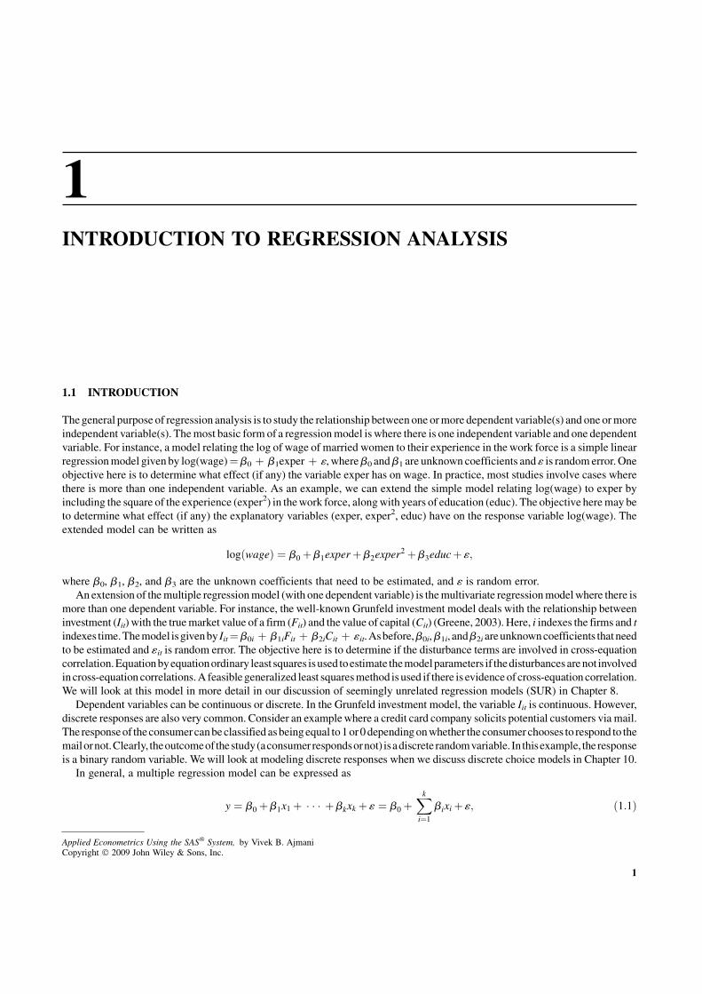
1INTRODUCTION TO REGRESSION ANALYSIS
1.1 INTRODUCTION
Thegeneral purpose of regression analysis is to study the relationship between one ormore dependent variable(s) and one ormore
independent variable(s). Themost basic form of a regressionmodel is where there is one independent variable and one dependent
variable. For instance, a model relating the log of wage of married women to their experience in thework force is a simple linear
regressionmodel given by log(wage)¼b0 þ b1exper þ «, whereb0 andb1 are unknown coefficients and « is randomerror.One
objective here is to determine what effect (if any) the variable exper has on wage. In practice, most studies involve cases where
there is more than one independent variable. As an example, we can extend the simple model relating log(wage) to exper by
including the square of the experience (exper2) in thework force, alongwith years of education (educ). The objective heremay be
to determine what effect (if any) the explanatory variables (exper, exper2, educ) have on the response variable log(wage). The
extended model can be written as
logðwageÞ ¼ b0 þb1experþb2exper2 þb3educþ «;
where b0, b1, b2, and b3 are the unknown coefficients that need to be estimated, and « is random error.
An extension of themultiple regressionmodel (with one dependent variable) is themultivariate regressionmodelwhere there is
more than one dependent variable. For instance, the well-known Grunfeld investment model deals with the relationship between
investment (Iit) with the truemarket value of a firm (Fit) and thevalue of capital (Cit) (Greene, 2003). Here, i indexes the firms and t
indexes time.Themodel isgivenby Iit¼b0i þ b1iFit þ b2iCit þ «it.Asbefore,b0i,b1i, andb2iareunknowncoefficients thatneed
to be estimated and «it is random error. The objective here is to determine if the disturbance terms are involved in cross-equation
correlation.Equationbyequationordinary least squares isused toestimate themodelparameters if thedisturbancesarenot involved
incross-equation correlations.A feasiblegeneralized least squaresmethod is used if there is evidenceof cross-equation correlation.
We will look at this model in more detail in our discussion of seemingly unrelated regression models (SUR) in Chapter 8.
Dependent variables can be continuous or discrete. In the Grunfeld investment model, the variable Iit is continuous. However,
discrete responses are also very common. Consider an examplewhere a credit card company solicits potential customers via mail.
The responseof theconsumercanbeclassified asbeingequal to1or0dependingonwhether theconsumer chooses to respond to the
mailornot.Clearly, theoutcomeof thestudy(aconsumerrespondsornot) isadiscrete randomvariable. In thisexample, the response
is a binary random variable. We will look at modeling discrete responses when we discuss discrete choice models in Chapter 10.
In general, a multiple regression model can be expressed as
y ¼ b0 þb1x1 þ � � � þbkxk þ « ¼ b0 þX
k
i¼1
bixi þ «; ð1:1Þ
1
Applied Econometrics Using the SAS� System, by Vivek B. AjmaniCopyright � 2009 John Wiley & Sons, Inc.

where y is the dependent variable, b0; . . . ;bk are the k þ 1 unknown coefficients that need to be estimated, x1; . . . ; xk are the kindependent or explanatory variables, and « is random error. Notice that the model is linear in parameters b0; . . . ;bk and is
therefore called a linear model. Linearity refers to how the parameters enter the model. For instance, the model
y ¼ b0 þb1x21 þ � � � þbkx
2k þ « is also a linear model. However, the exponential model y¼b0 exp(�xb1) is a nonlinear model
since the parameter b1 enters the model in a nonlinear fashion through the exponential function.
1.1.1 Interpretation of the Parameters
One of the assumptions (to be discussed later) for the linear model is that the conditional expectationE(«jx1; . . . ; xk) equals zero.Under this assumption, the expectation, Eðyjx1; . . . ; xkÞ can be written as Eðyjx1; . . . ; xkÞ ¼ b0 þ
Pki¼1 bixi. That is, the
regressionmodel can be interpreted as the conditional expectation of y for givenvalues of the explanatory variables x1; . . . ; xk. IntheGrunfeld example, we could discuss the expected investment for a given firm for knownvalues of the firm�s truemarket value
and value of its capital. The intercept term, b0, gives the expected value of ywhen all the explanatory variables are set at zero. In
practice, this rarely makes sense since it is very uncommon to observe values of all the explanatory variables equal to zero.
Furthermore, the expected value of y under such a casewill often yield impossible results. The coefficient bk is interpreted as the
expected change in y for a unit change in xk holding all other explanatory variables constant. That is, ¶E(yjx1; . . . ; xk)=¶xk¼bk.
The requirement that all other explanatory variables be held constant when interpreting a coefficient of interest is called the
ceteris paribus condition. The effect of xk on the expected value of y is referred to as the marginal effect of xk.
Economists are typically interested in elasticities rather thanmarginal effects. Elasticity is defined as the relative change in the
dependent variable for a relative change in the independent variable. That is, elasticity measures the responsiveness of one
variable to changes in another variable—the greater the elasticity, the greater the responsiveness.
There is a distinction between marginal effect and elasticity. As stated above, the marginal effect is simply ¶E(yjxÞ=¶xkwhereas elasticity is defined as the ratio of the percentage change in y to the percentage change in x. That is, e ¼ ð¶y=yÞ=ð¶xk=xkÞ.
Consider calculating the elasticity of x1 in the general regression model given by Eq. (1.1). According to the definition of
elasticity, this is given by ex1 ¼ ð¶y=¶x1Þðx1=yÞ ¼ b1ðx1=yÞ 6¼ b1. Notice that the marginal effect is constant whereas the
elasticity is not. Next, consider calculating the elasticity in a log–log model given by log(y)¼b0 þ b1 log(x) þ «. In this case,
elasticity of x is given by
¶ logðyÞ ¼ b1¶ logðxÞ ) ¶y1
y¼ b1¶x
1
x)
¶y
¶x
x
y¼ b1:
Themarginal effect for the log–logmodel is alsob1. Next, consider the semi-logmodel given by y¼b1 þ b1 log(x) þ «. In this
case, elasticity of x is given by
¶y ¼ b1¶ logðxÞ ) ¶y ¼ b1¶x1
x)
¶y
¶x
x
y¼ b1
1
y:
On the other hand, the marginal effect in the semi-log model is given by b1(1=x).For the semi-log model given by logðyÞ ¼ b0 þ b1xþ «, the elasticity of x is given by
¶y logðyÞ ¼ b1¶x ) ¶y1
y¼ b1¶x ¼
¶y
¶x
x
y¼ b1x:
On the other hand, the marginal effect in the semi-log model is given by b1y.
Mostmodels that appear in this bookhavea log transformationon the dependent variable or the independent variable or both. It
may be useful to clarify how the coefficients from these models are interpreted. For the semi-log model where the dependent
variable has been transformed using the log transformation while the explanatory variables are in their original units, the
coefficient b is interpreted as follows: For a one unit change in the explanatory variable, the dependent variable changes by
b�100% holding all other explanatory variables constant.
In the semi-logmodelwhere the explanatory variable has been transformedbyusing the log transformation, the coefficientb is
interpreted as follows: For a one unit change in the explanatory variable, the dependent variable increases (decreases) by
b/100 units.
In the log–logmodelwhere both the dependent and independent variable havebeen transformed byusing a log transformation,
the coefficient b is interpreted as follows: A 1% change in the explanatory variable is associated with a b% change in the
dependent variable.
2 INTRODUCTION TO REGRESSION ANALYSIS

1.1.2 Objectives and Assumptions in Regression Analysis
There are three main objectives in any regression analysis study. They are
a. To estimate the unknown parameters in the model.
b. To validate whether the functional form of the model is consistent with the hypothesized model that was dictated by theory.
c. To use the model to predict future values of the response variable, y.
Most regression analysis in econometrics involves objectives (a) and (b). Econometric time series analysis involves all
three. There are five key assumptions that need to be checked before the regressionmodel can be used for the purposes outlined
above.
a. Linearity: The relationship between the dependent variable y and the independent variables x1; . . . ; xk is linear.
b. Full Rank: There is no linear relationship among any of the independent variables in the model. This assumption is often
violated when the model suffers from multicollinearity.
c. Exogeneity of the Explanatory Variables:This implies that the error term is independent of the explanatory variables. That
is,E(«ijxi1; xi2; . . . ; xik)¼ 0. This assumption states that the underlyingmechanism that generated the data is different from
the mechanism that generated the errors. Chapter 4 deals with alternative methods of estimation when this assumption is
violated.
d. Random Errors: The errors are random, uncorrelated with each other, and have constant variance. This assumption is
called the homoscedasticity and nonautocorrelation assumption. Chapters 5 and 6 deal with alternative methods of
estimation when this assumption is violated. That is estimation methods when the model suffers from heteroscedasticity
and serial correlation.
e. Normal Distribution: The distribution of the random errors is normal. This assumption is used in making inference
(hypothesis tests, confidence intervals) to the regression parameters but is not needed in estimating the parameters.
1.2 MATRIX FORM OF THE MULTIPLE REGRESSION MODEL
The multiple regression model in Eq. (1.1) can be expressed in matrix notation as y¼Xb þ e. Here, y is an n� 1 vector of
observations,X is a n� (kþ 1)matrix containing values of explanatory variables,b is a (kþ 1)� 1 vector of coefficients, and e is
an n� 1 vector of random errors. Note that X consists of a column of 1’s for the intercept term b0. The regression analysis
assumptions, in matrix notation, can be restated as follows:
a. Linearity: y¼b0þ x1b1 þ � � � þ xkbk þ e or y¼Xb þ e.
b. Full Rank: X is an n� (kþ 1) matrix with rank (kþ 1).
c. Exogeneity: E(ejX)¼ 0 � X is uncorrelated with e and is generated by a process that is independent of the process that
generated the disturbance.
d. Spherical Disturbances: Var(«ijX)¼s2 for all i¼ 1; . . . ; n and Cov(«i,«jjX)¼ 0 for all i 6¼ j. That is, VarðejXÞ ¼ s2I.
e. Normality: ejX�N(0,s2I).
1.3 BASIC THEORY OF LEAST SQUARES
Least squares estimation in the simple linear regression model involves finding estimators b0 and b1 that minimize the sums of
squares L ¼ Sni¼1ðyi �b0 �b1xiÞ
2. Taking derivatives of L with respect to b0 and b1 gives
¶L
¶b0
¼ �2X
n
i¼1
ðyi�b0�b1xiÞ;
¶L
¶b1
¼ �2X
n
i¼1
ðyi�b0�b1xiÞxi:
BASIC THEORY OF LEAST SQUARES 3

Equating the two equations to zero and solving for b0 and b1 gives
X
n
i¼1
yi ¼ nb0 þ b1
X
n
i¼1
xi;
X
n
i¼1
yixi ¼ b0
X
n
i¼1
xi þ b1
X
n
i¼1
x2i :
These two equations are known as normal equations. There are twonormal equations and twounknowns. Therefore, we can solve
these to get the ordinary least squares (OLS) estimators ofb0 andb1. The first normal equation gives the estimator of the intercept,
b0, b0 ¼ �y�b1�x. Substituting this in the second normal equation and solving for b1 gives
b1 ¼
nP
n
i¼1
yixi �P
n
i¼1
yiP
n
i¼1
xi
nP
n
i¼1
x2i �P
n
i¼1
xi
� �2:
Wecan easily extend this to themultiple linear regressionmodel inEq. (1.1). In this case, least squares estimation involves finding
an estimator b of b to minimize the error sums of squares L¼ (y�Xb)T(y�Xb). Taking the derivative of L with respect to b
yields kþ 1 normal equations with kþ 1 unknowns (including the intercept) given by
¶L=¶b ¼ �2ðXTy�XTXbÞ:
Setting this equal to zero and solving for b gives the least squares estimator ofb, b¼ (XTX)�1XTy. A computational form for b is
given by
b ¼X
n
i¼1
xTi xi
!�1X
n
i¼1
xTi yi
!
:
The estimated regression model or predicted value of y is therefore given by y ¼ Xb. The residual vector e is defined as the
difference between the observed and the predicted value of y, that is, e ¼ y�y.
The method of least squares produces unbiased estimates of b. To see this, note that
EðbjXÞ ¼ EððXTXÞ�1XTyjXÞ
¼ ðXTXÞ�1XTEðyjXÞ
¼ ðXTXÞ�1XTEðXbþ ejXÞ
¼ ðXTXÞ�1XTXbEðejXÞ
¼b:
Here, we made use of the fact that (XTX)�1¼ (XTX)¼ I, where I is the identity matrix and the assumption that E(ejX)¼ 0.
1.3.1 Consistency of the Least Squares Estimator
First, note that a consistent estimator is an estimator that converges in probability to the parameter being estimated as the sample
size increases. To say that a sequence of random variables Xn converges in probability to X implies that as n ! ¥ the probability
that jXn�Xj � d is zero for all d (Casella and Berger, 1990). That is,
limn!¥
PrðjXn �Xj � dÞ ¼ 0 8 d:
Under the exogeneity assumption, the least squares estimator is a consistent estimator of b. That is,
limn!¥
Prðjbn�bj � dÞ ¼ 0 8 d:
To see this, let xi, i¼ 1; . . . ; n; be a sequence of independent observations and assume that XTX/n converges in probability to a
positive definite matrix C. That is (using the probability limit notation),
p limn!¥
XTX
n¼ C:
4 INTRODUCTION TO REGRESSION ANALYSIS

Note that this assumption allows the existence of the inverse of XTX . The least squares estimator can then be written as
b ¼ bþXTX
n
� ��1XT
e
n
� �
:
Assuming that C�1 exists, we have
p limb ¼ bþC�1p lim
XTe
n
� �
:
Inorder to showconsistency,wemust show that the second term in this equationhas expectation zero and avariance that converges
to zero as the sample size increases.Under the exogeneity assumption, it is easy to show thatE(XTejX)¼ 0 sinceE(ejX)¼ 0. It can
also be shown that the variance of XTe=n is
VarXT
e
n
� �
¼s2
nC:
Therefore, as n ! ¥ the variance converges to zero and thus the least squares estimator is a consistent estimator for b (Greene,
2003, p. 66).
Moving on to the variance–covariance matrix of b, it can be shown that this is given by
VarðbjXÞ ¼ s2ðXTXÞ�1:
To see this, note that
VarðbjXÞ¼ VarððXTXÞ�1XTyjXÞ
¼ VarððXTXÞ�1XTðXbþ eÞjXÞ
¼ ðXTXÞ�1XTVarðejXÞXðXTXÞ�1
¼ s2ðXTXÞ�1:
It can be shown that the least squares estimator is the best linear unbiased estimator of b. This is based on the well-known result,
called the Gauss–Markov Theorem, and implies that the least squares estimator has the smallest variance in the class of all
unbiased estimators of b (Casella and Berger, 1990; Greene, 2003; Meyers, 1990).
An estimator ofs2 can be obtained by considering the sums of squares of the residuals (SSE). Here, SSE¼ (y�Xb)T(y�Xb).
Dividing SSE by its degrees of freedom, n� k� 1 yields s2. That is, the mean square error is given by
s2 ¼ MSE ¼ SSE=ðn�k�1Þ. Therefore, an estimate of the covariance matrix of b is given by s2ðXTXÞ�1.
Using a similar argument as the one used to showconsistencyof the least squares estimator, it can be shown that s2 is consistent
fors2 and that the asymptotic covariance matrix of b is s2ðXTXÞ�1(see Greene, 2003, p. 69 for more details). The square root of
the diagonal elements of this yields the standard errors of the individual coefficient estimates.
1.3.2 Asymptotic Normality of the Least Squares Estimator
Using the properties of the least squares estimator given in Section 1.3 and the Central Limit Theorem, it can be easily shown that
the least squares estimator has an asymptotic normal distribution with mean b and variance–covariance matrixs2(XTX)�1. That
is, b � asym:N�
b;s2ðXTXÞ�1�
.
1.4 ANALYSIS OF VARIANCE
The total variability in the data set (SST) can be partitioned into the sums of squares for error (SSE) and the sums of squares for
regression (SSR). That is, SST¼ SSE þ SSR. Here,
SST ¼ yTy�
X
n
i¼1
yi
!2
n;
SSE ¼ yTy�bTXTy;
SSR ¼ bTXTy�
X
n
i¼1
yi
!2
n:
ANALYSIS OF VARIANCE 5

TABLE 1.1. Analysis of Variance Table
Source of
Variation
Sums of
Squares
Degrees of
Freedom Mean Square F0
Regression SSR k MSR¼ SSR/k
Error SSE n� k�1 MSE¼ SSE/(n� k�1)
Total SST n� 1 MSR/MSE
The mean square terms are simply the sums of square terms divided by their degrees of freedom. We can therefore write the
analysis of variance (ANOVA) table as given in Table 1.1.
The F statistic is the ratio between the mean square for regression and the mean square for error. It tests the global hypotheses
H0: b1 ¼ b2 ¼ . . . ¼ bk ¼ 0;
H1: At least one bi 6¼ 0 for i ¼ 1; . . . ; k:
Thenull hypothesis states that there is no relationshipbetween the explanatoryvariables and the responsevariable. The alternative
hypothesis states that at least one of the k explanatory variables has a significant effect on the response. Under the assumption that
the null hypothesis is true,F0 has anF distribution with k numerator and n� k�1 denominator degrees of freedom, that is, under
H0, F0�Fk,n�k�1. The p value is defined as the probability that a random variable from the F distribution with k numerator and
n� k�1 denominator degrees of freedom exceeds the observed value of F, that is, Pr(Fk,n�k�1>F0). The null hypothesis is
rejected in favor of the alternative hypothesis if the p value is less than a, where a is the type I error.
1.5 THE FRISCH–WAUGH THEOREM
Often, wemay be interested only in a subset of the full set of variables included in themodel. Consider partitioningX intoX1 and
X2. That is, X¼ [X1 X2]. The general linear model can therefore be written as y¼Xb þ e¼X1b1 þ X2b2 þ e. The normal
equations can be written as (Greene, 2003, pp. 26–27; Lovell, 2006)
XT1X1 XT
1X2
XT2X1 XT
2X2
" #"
b1
b2
#
¼XT
1y
XT2y
" #
:
It can be shown that
b1 ¼ ðXT1X1Þ
�1XT
1 ðy�X2b2Þ:
IfXT1X2 ¼ 0, then b1 ¼ ðXT
1X1Þ�1XT
1y. That is, if the matricesX1 andX2 are orthogonal, then b1 can be obtained by regressing y
on X1. Similarly, b2 can be obtained by regressing y on X2. It can easily be shown that
b2 ¼ ðXT2M1X2Þ
�1ðXT2M1yÞ;
where M1 ¼ ðI�X1ðXT1X1Þ
�1XT
1 Þ so that M1y is a vector of residuals from a regression of y on X1.
Note thatM1X2 is amatrix of residuals obtained by regressingX2 onX1. The computations described here form the basis of the
well-knownFrisch–WaughTheorem,which states thatb2 can be obtained by regressing the residuals from a regression of y onX1
with the residuals obtained by regressingX2onX1.One application of this result is in the derivation of the formof the least squares
estimators in the fixed effects (LSDV) model, which will be discussed in Chapter 7.
1.6 GOODNESS OF FIT
Two commonly used goodness-of-fit statistics used are the coefficient of determination (R2) and the adjusted coefficient of
determination (R2A). R
2 is defined as
R2 ¼SSR
SST¼ 1�
SSE
SST:
6 INTRODUCTION TO REGRESSION ANALYSIS

It measures the amount of variability in the response, y, that is explained by including the regressors x1; x2; . . . ; xk in the model.
Due to the nature of its construction, we have 0�R2� 1. Although higher values (values closer to 1) are desired, a large value
of R2 does not necessarily imply that the regression model is a good one. Adding a variable to the model will always increase
R2 regardless of whether the additional variable is statistically significant or not. In other words,R2 can be artificially inflated by
overfitting the model.
To see this, consider themodel y¼X1b1þ X2b2þU. Here, y is a n�1 vector of observations,X1 is the n� k1 datamatrixb1
is a vector of k1 coefficients,X2is the n� k2 data matrix with k2 added variables, b2 is a vector of k2 coefficients, andU is a n�1
random vector. Using the Frisch–Waugh theorem, we can show that
b2 ¼�
XT2MX2
��1XT
2My ¼�
X2*T X2*
��1X2*T y*:
Here,X2* ¼ MX2; y* ¼ My, andM ¼ I�X1ðXT1X1Þ
�1XT
1 . That is,X2* and y* are residual vectors of the regression ofX2 and
y on X1. We can invoke the Frisch–Waugh theorem again to get an expression for b1. That is, b1 ¼�
XT1X1
��1XT
1
�
y�X2 b2
�
.
Using elementary algebra, we can simplify this expression to get b1 ¼ b��
XT1X1
��1XT
1X2 b2, where b ¼�
XT1X1
��1XT
1y.
Next, note that u ¼ y�X1 b1�X2 b2. We can substitute the expression of b1 in this to get U ¼ u ¼ e�MX2b2 ¼ e�X2*b2. The
sums of squares of error for the extra variable model is therefore given by
uTu ¼ eTeþ bT2
�
XT2*X2*
�
b2�2b2XT2*e ¼ eTe þ bT
2
�
XT2*X2*
�
b2�2bT2X
T2*y*:
Here, e is the residual y�X1b or My¼ y*. We can now, manipulate b2 to get
XT2*y* ¼
�
XT2*X2*
�
b2 and
uTu ¼ eTe�bT2
�
XT2*X2*
�
b2 � eTe:
Dividing both sides by the total sums of squares, yTM0y, we get
uTu
yTM0y�
eTe
yTM0y) R2
X1;X2� R2
X1;
whereM0¼ I� i(iTi)�1 iT. See Greene (2003, p. 30) for a proof for the casewhen a single variable is added to an existingmodel.
Thus, it is possible for models to have a high R2 yet yield poor predictions of new observations for the mean response. It is for
this reason thatmanypractitioners also use the adjusted coefficient of variation,R2A,which adjustsR
2with respect to the number of
explanatory variables in the model. It is defined as
R2A ¼ 1�
SSE=ðn�k�1Þ
SST=ðn�1Þ¼ 1�
n�1
n�k�1
� �
ð1�R2Þ:
In general, it will increase onlywhen significant terms that improve themodel are added to themodel. On the other hand, it will
decreasewith the addition of nonsignificant terms to themodel. Therefore, it will always be less than or equal toR2.When the two
R2 measures differ dramatically, there is a good chance that nonsignificant terms have been added to the model.
1.7 HYPOTHESIS TESTING AND CONFIDENCE INTERVALS
The global F test checks the hypothesis that at least one of the k regressors has a significant effect on the response. It does not
indicatewhich explanatory variable has an effect. It is therefore essential to conduct hypothesis tests on the individual coefficients
bj(j¼ 1; . . . ; k). The hypothesis statements are H0:bj¼ 0 and H1:bj 6¼ 0. The test statistic for testing this is the ratio of the least
squares estimate and the standard error of the estimate. That is,
t0 ¼bj
s:e:ðbjÞ; j ¼ 1; . . . ; k;
HYPOTHESIS TESTING AND CONFIDENCE INTERVALS 7

where s.e.(bj) is the standard error associated with bj and is defined as s:e:ðbjÞ ¼ffiffiffiffiffiffiffiffiffiffiffi
s2Cjj
q
, where Cjj is the jth diagonal element
of (XTX)�1 corresponding to bj. Under the assumption that the null hypothesis is true, the test statistic t0 is distributed as a
tdistributionwithn� k� 1degrees of freedom.That is, t0� tn�k� 1. Thepvalue is defined as before. That is, Pr(jt0j>tn�k� 1).We
reject thenull hypothesis if thepvalue<a,wherea is the type I error.Note that this test is amarginal test sincebjdependsonall the
other regressors xi(i 6¼ j) that are in the model (see the earlier discussion on interpreting the coefficients).
Hypothesis tests are typically followed by the calculation of confidence intervals. A 100(1�a)% confidence interval for the
regression coefficient bj(j¼ 1; . . . ; k) is given by
bj�ta=2;n�k�1s:e:ðbjÞ � bj � bj þ ta=2;n�k�1s:e:ðbjÞ:
Note that these confidence intervals can also be used to conduct the hypothesis tests. In particular, if the range of values for the
confidence interval includes zero, then we would fail to reject the null hypothesis.
Two other confidence intervals of interest are the confidence interval for themean responseEðyjx0Þ and the prediction intervalfor an observation selected from the conditional distribution f ðyjx0Þ, where without loss of generality f ð*Þ is assumed to be
normally distributed. Also note that x0 is the setting of the explanatory variables at which the distribution of y needs to be
evaluated. Notice that the mean of y at a given value of x¼ x0 is given by Eðyjx0Þ ¼ xT0b.
An unbiased estimator for themean response is x0Tb. That is,E(x0
TbjX)¼ x0Tb. It can be shown that the variance of this unbiased
estimator is given by s2xT0 ðXTXÞ�1
x0. Using the previously defined estimator for s2 (see Section 1.3.1 ), we can construct a
100(1� a)% confidence interval on the mean response as
yðx0Þ� ta=2;n�k�1
ffiffiffiffiffiffiffiffiffiffiffiffiffiffiffiffiffiffiffiffiffiffiffiffiffiffiffiffiffiffiffiffi
s2xT0 ðXTXÞ�1
x0
q
� myjx0 � yðx0Þþ ta=2;n�k�1
ffiffiffiffiffiffiffiffiffiffiffiffiffiffiffiffiffiffiffiffiffiffiffiffiffiffiffiffiffiffiffiffi
s2xT0 ðXTXÞ�1
x0
q
:
Using a similar method, one can easily construct a 100(1�a)% prediction interval for a future observation x0 as
yðx0Þ� ta=2;n�k�1
ffiffiffiffiffiffiffiffiffiffiffiffiffiffiffiffiffiffiffiffiffiffiffiffiffiffiffiffiffiffiffiffiffiffiffiffiffiffiffiffiffiffiffi
s2ð1þ xT0 ðXTXÞ�1
x0Þ
q
� yðx0Þ � yðx0Þþ ta=2;n�k�1
ffiffiffiffiffiffiffiffiffiffiffiffiffiffiffiffiffiffiffiffiffiffiffiffiffiffiffiffiffiffiffiffiffiffiffiffiffiffiffiffiffiffiffi
s2ð1þ xT0 ðXTXÞ�1
x0Þ
q
:
In both these cases, the observation vector x0 is defined as x0¼ (1; x01; x02; . . . ; x0k), where the “1” is added to account for the
intercept term.
Notice that the width of the prediction interval at point x0 is wider than the width of the confidence interval for the mean
response atx0. This is easy to see because the standard error used for the prediction interval is larger than the standard error used for
themean response interval. This shouldmake intuitive sense also since it is easier to predict themean of a distribution than it is to
predict a future value from the same distribution.
1.8 SOME FURTHER NOTES
Akey step in regression analysis is residual analysis to check the least squares assumptions. Violation of one ormore assumptions
can render the estimation and any subsequent hypothesis tests meaningless. As stated earlier, the least squares residuals can be
computed as e¼ y�Xb. Simple residual plots can be used to check a number of assumptions.Chapter 2 shows how these plots are
constructed. Here, we simply outline the different types of residual plots that can be used.
1. A plot of the residuals in time order can be used to check for the presence of autocorrelation. This plot can also be used to
check for outliers.
2. A plot of the residuals versus the predicted value can be used to check the assumption of random, independently distributed
errors. This plot (and the residuals versus regressors plots) can be used to check for the presence of heteroscedasticity. This
plot can also be used to check for outliers and influential observations.
3. The normal probability plot of the residuals can be used to check any violations from the assumption of normally
distributed random errors.
8 INTRODUCTION TO REGRESSION ANALYSIS

2REGRESSIONANALYSIS USING PROC IML AND PROCREG
2.1 INTRODUCTION
We discussed basic regression concepts and least squares theory in Chapter 1. This chapter deals with conducting regression
analysis calculations in SAS.Wewill show the computations by using both Proc IML and Proc Reg. Even though the results from
both procedures are identical, usingProc IMLallows one to understand themechanics behind the calculations thatwere discussed
in the previous chapter. Freund and Littell (2000) offer an in-depth coverage of how SAS can be used to conduct regression
analysis in SAS. This chapter discusses the basic elements of Proc Reg as it relates to conducting regression analysis.
To illustrate the computations in SAS, we will make use of the investment equation data set provided in Greene (2003). The
source of the data is attributed to the Economic Report of the President published by the U.S. Government Printing Office in
Washington, D.C. The author�s description of the problem appears on page 21 of his text and is summarized here. The objective is
to estimate an investment equation by usingGNP (gross national product), and a time trend variableT. Note thatT is not part of the
original data set but is created in the data step statement in SAS. Initially, we ignore the variables Interest Rate and Inflation Rate
since our purpose here is to illustrate how the computations canbe carried out usingSAS.Additional variables canbe incorporated
into the analysis with a few minor modifications of the program. We will first discuss conducting the analysis in Proc IML.
2.2 REGRESSION ANALYSIS USING PROC IML
2.2.1 Reading the Data
The source data can be read in a number of different ways.We decided to create temporary SAS data sets from the raw data stored
in Excel. However, we could easily have entered the data directly within the data step statement since the size of data set is small.
The Proc Import statement reads the raw data set and creates a SAS temporary data set named invst_equation. Using the approach
taken byGreene (2003), the data step statement that follows creates a trend variableT, and it also converts thevariables investment
and GNP to real terms by dividing them by the CPI (consumer price index). These two variables are then scaled so that the
measurements are now scaled in terms of trillions of dollars. In a subsequent example,wewillmake full use of the investment data
set by regressing real investment against a constant, a trend variable, GNP, interest rate, and inflation rate that is computed as a
percentage change in the CPI.
proc import out=invst_equation
datafile="C:\Temp\Invest_Data"
dbms=Excel
9
Applied Econometrics Using the SAS� System, by Vivek B. AjmaniCopyright � 2009 John Wiley & Sons, Inc.

replace;
getnames=yes;
run;
data invst_equation;
set invst_equation;
T=_n_;
Real_GNP=GNP/CPI*10);
Real_Invest=Invest/(CPI*10);
run;
2.2.2 Analyzing the Data Using Proc IML
Proc IML begins with the statement “Proc IML;” and ends with the statement “Run;”. The analysis statements are written
between these two. The first step is to read the temporary SAS data set variables into a matrix. In our example, the data matrix
X contains two columns: T and Real_GNP. Of course, we also need a column of 1�s to account for the intercept term. The
response vector y contains the variable Real_Invest. The following statements are needed to create the data matrix and the
response vector.
use invst_equation;
read all var {’T’ ’Real_GNP’} into X;
read all var {’Real_Invest’} into Y;
Note that the model degrees of freedom are the number of columns of X excluding the column of 1�s. Therefore, it is a
good idea to store the number of columns in X at this stage. The number of rows and columns of the data matrix are
calculated as follows:
n=nrow(X);
k=ncol(X);
A column of 1�s is now concatenated to the data matrix to get the matrix in analysis ready format.
X=J(n,1,1)||X;
The vector of coefficients can now easily be calculated by using the following set of commands:
C=inv(X‘*X);
B_Hat=C*X‘*Y;
Note that we decided to compute (XT X)�1 separately since this matrix is used frequently in other computations, and it is
convenient to have it calculated just once and ready to use.
With the coefficient vector computed, we can now focus our attention on creating the ANOVA table. The following
commands compute the sums of squares (regression, error, total), the error degrees of freedom, the mean squares, and the F
statistic.
SSE=y‘*y-B_Hat‘*X‘*Y;
DFE=n-k-1;
MSE=SSE/DFE;
Mean_Y=Sum(Y)/n;
SSR=B_Hat‘*X‘*Y-n*Mean_Y**2;
MSR=SSR/k;
SST=SSR+SSE;
F=MSR/MSE;
Next, we calculate the coefficient of determination (R2) and the adjusted coefficient of determination (adj R2).
10 REGRESSION ANALYSIS USING PROC IML AND PROC REG

R_Square=SSR/SST;
Adj_R_Square=1-(n-1)/(n-k-1) * (1-R_Square);
We also need to calculate the standard errors of the regression estimates in order to compute the t-statistic values and the
corresponding p values. The function PROBTwill calculate the probability that a random variable from the t distribution with df
degrees of freedom will exceed a given t value. Since the function takes in only positive values of t, we need to use the absolute
value function abs. The value obtained is multiplied by ‘2’ to get the p value for a two-sided test.
SE=SQRT(vecdiag(C)#MSE);
T=B_Hat/SE;
PROBT=2*(1-CDF(’T’, ABS(T), DFE));
With the key statistics calculated, we can start focusing our attention on generating the output. We have found the
following set of commands useful in creating a concise output.
ANOVA_Table=(k||SSR||MSR||F)//(DFE||SSE||MSE||{.});
STATS_Table=B_Hat||SE||T||PROBT;
Print ’Regression Results for the Investment
Equation’;
Print ANOVA_Table (|Colname={DF SS MS F} rowname={Model
Error} format=8.4|);
Print ’Parameter Estimates’;
Print STATS_Table (|Colname={BHAT SE T PROBT} rowname={INT
T Real_GNP} format=8.4|);
Print ’The value of R-Square is ’ R_Square; (1 format = 8.41);
Print ’The value of Adj R-Square is ’ Adj_R_Square;
(1 format = 8.41);
These statements produce the results given in Output 2.1. The results of the analysis will be discussed later.
Regression Results for the Investment Equation
ANOVA_TABLE
DF SS MS F
MODEL 2.0000 0.0156 0.0078 143.6729
ERROR 12.0000 0.0007 0.0001 .
Parameter Estimates
STATS_TABLE
BHAT SE T PROBT
INT -0.5002 0.0603 -8.2909 0.0000
T -0.0172 0.0021 -8.0305 0.0000
REAL_GNP 0.6536 0.0598 10.9294 0.0000
R_SQUARE
The value of R-Square is 0.9599
ADJ_R_SQUARE
The value of Adj R-Square is 0.9532
OUTPUT 2.1. Proc IML analysis of the investment data.
REGRESSION ANALYSIS USING PROC IML 11

2.3 ANALYZING THE DATA USING PROC REG
This section deals with analyzing the investment data using Proc Reg. The general form of the statements for this procedure is
Proc Reg Data=dataset;
Model Dependent Variable(s) = Independent Variable(s)/Model
Options;
Run;
SeeFreund andLittell (2000) for details onother options for ProcRegand their applications.Wewillmakeuse of only a limited
set of options that will help us achieve our objectives. The dependent variable in the investment data is Real Investment, and the
independent variables are Real GNP and the time trend T. The SAS statements required to run the analysis are
Proc Reg Data=invst_equation;
Model Real_Invest=Real_GNP T;
Run;
The analysis results are given in Output 2.2. Notice that the output from Proc Reg matches the output from Proc IML.
2.3.1 Interpretation of the Output (Freund and Littell, 2000, pp. 17–24)
The first few lines of the output display the name of the model (Model 1, which can be changed to a more appropriate name), the
dependent variable, and the number of observations read and used. These two values will be equal unless there are missing
observations in the data set for either the dependent or the independent variables or both. The investment equation data set has a
total of 15 observations and there are no missing observations.
The analysis of variance table lists the standard output one would expect to find in an ANOVA table: the sources of variation,
the degrees of freedom, the sums of squares for the different sources of variation, the mean squares associated with these, the
The REG ProcedureModel: MODEL1
Dependent Variable: Real_Invest
The REG ProcedureModel: MODEL1
Dependent Variable: Real_Invest
Number of Observations Read 15
Number of Observations Used 15
Analysis of Variance
Source DFSum ofSquares
MeanSquare F Value Pr > F
Model 2 0.01564 0.00782 143.67 <0.0001
Error 12 0.00065315 0.00005443
Corrected Total 14 0.01629
Root MSE 0.00738 R-Square 0.9599
Dependent Mean 0.20343 Adj R-Sq 0.9532
Coeff Var 3.62655
Parameter Estimates
Variable DFParameterEstimate
StandardError t Value Pr > |t|
Intercept 1 -0.50022 0.06033 -8.29 <0.0001
<0.0001
<0.0001Real_GNP 1 0.65358 0.05980 10.93
T 1 -0.01721 0.00214 -8.03
OUTPUT 2.2. Proc Reg analysis of the investment data.
12 REGRESSION ANALYSIS USING PROC IML AND PROC REG

F-statistic value, and the pvalue.As discussed inChapter 1, the degrees of freedom for themodel are k, the number of independent
variables, which in this example is 2. The degrees of freedom for the error sums of squares are n� k� 1,which is 15� 2� 1or 12.
The total degrees of freedom are the sum of the model and error degrees of freedom or n� 1, the number of nonmissing
observations minus one. In this example, the total degrees of freedom are 14.
i. In Chapter 1, we saw that the total sums of squares can be partitioned into themodel and the error sums of squares. That is,
the Corrected Total Sums of Squares¼Model Sums of Squares þ Error Sums of Squares. From theANOVA table, we see
that 0.01564 þ 0.00065 equals 0.01629.
ii. Themean squares are calculated by dividing the sums of squares by their corresponding degrees of freedom. If themodel is
correctly specified, then themean square for error is an unbiased estimate ofs2, the variance of e, and the error term of the
linear model. From the ANOVA table,
MSR ¼ 0:01564
2¼ 0:00782
and
MSE ¼ 0:00065315
12¼ 0:00005443:
iii. The F-statistic value is the ratio of the mean square for regression and the mean square for error. From the ANOVA table,
F ¼ 0:00782
0:00005443¼ 143:67:
It tests the hypothesis that
H0 : b1 ¼ b2 ¼ 0;
H1 : At least one of the b’s 6¼ 0:
Here,b1 andb2 are the true regression coefficients for Real GNP and Trend. Under the assumption that the null hypothesis
is true,
F ¼ MSR
MSE� F2;12
and the
p value ¼ PrðF > F2;12Þ ¼ PrðF > 143:67Þ � 0:
The p value indicates that there is almost no chance of obtaining anF-statistic value as high or higher than 143.67 under the
null hypothesis. Therefore, the null hypothesis is rejected and we claim that the overall model is significant.
The root MSE is the square root of the mean square error and is an estimate of the standard deviation of
eðffiffiffiffiffiffiffiffiffiffiffiffiffiffiffiffiffiffiffiffiffiffiffi
0:00005443p
¼ 0:00738Þ. The dependent mean is simply the mean of the dependent variable Real Invest. Coeff Var is the
coefficient of variation and is defined as
root�mse
dependent�mean� 100:
As discussed inMeyers (1990, p. 40), this statistic is scale free and can therefore be used in place of the root mean square error
(which is not scale free) to assess the quality of the model fit. To see how this is interpreted, consider the investment data set
example. In this example, the coefficient of variation is 3.63%, which implies that the dispersion around the least squares line as
measured by the root mean square error is 3.63% of the overall mean of Real Invest.
ANALYZING THE DATA USING PROC REG 13

The coefficient of determination (R2) is 96%. This implies that the regression model explains 96% of the variation in the
dependent variable. As explained in Chapter 1, it is calculated by dividing themodel sums of squares by the total sums of squares
and expressing the result as a percentage (0.01564/0.01629¼ 0.96). The adjusted R2 value is an alternative to the R2 value and
takes the number of parameters into account. In our example, the adjusted R2¼ 95.32%. This is calculated as
R2A ¼ 1� SSE=ðn�k�1Þ
SST=ðn�1Þ ¼ 1�
n�1
n�k�1
!
ð1�R2Þ
¼ 1� 14
12� ð1� 0:96Þ ¼ 0:9533:
Notice that the values of R2 and adjusted R2 are very close.
The parameter estimates table lists the intercept and the independent variables along with the estimated values of the
coefficients, their standard errors, the t-statistic values, and the p values.
i. The first column gives the estimated values of the regression coefficients. From these, we canwrite the estimatedmodel as
Estimated Real_Invest¼�0.50 þ 0.65 Real_GNP – 0.017 T.
The coefficient for Real_GNP is positive, indicating a positive correlation between it and Real_Invest. The coefficient
value of 0.65 indicates that an increase of one trillion dollars of Real GNPwould lead to an average of 0.65 trillion dollars
of Real Investment (Greene, 2003). Here, we have to assume that Time (T) is held constant.
ii. The standard error column gives the standard errors for the coefficient estimates. These values are the square root of the
diagonal elements of s2ðXT XÞ�1. These are used to conduct hypothesis tests for the regression parameters and to
construct confidence intervals.
iii. The t value column lists the t statistics used for testing
H0 : bi ¼ 0;
H1 : bi 6¼ 0; i ¼ 1; 2:
These are calculatedbydividing the estimatedcoefficient valuesby their corresponding standarderror values. For example, the
t value corresponding to the coefficient forReal_GNP is 0.65358/0.05980¼ 10.93. The last column gives the p values associated
with the t-test statistic values.As anexample, thepvalue forReal_GNP is givenbyP(j t j>10.93).Using the t tablewith12degrees
of freedom,we see that thepvalue forReal_GNP is zero, indicating high significance. In the real investment example, thepvalues
for both independent variables offer strong evidence against the null hypothesis.
2.4 EXTENDING THE INVESTMENT EQUATION MODEL TO THE COMPLETE DATA SET
We will now extend this analysis by running a regression on the complete Investment Equation data set. Note that the CPI in
1967 was recorded as 79.06 (Greene, 2003, p. 947) and that Inflation Rate is defined as the percentage change in CPI. The
following data step gets the data in analysis-ready format.
Data invst_equation;
set invst_equation;
T=_n_;
Real_GNP=GNP/(CPI*10);
Real_Invest=Invest/(CPI*10);
CPI0=79.06;
Inflation_Rate=100*((CPI-Lag(CPI))/Lag(CPI));
if inflation_rate=. then inflation_rate=100*((CPI-
79.06)/79.06);
drop Year GNP Invest CPI CPI0;
run;
14 REGRESSION ANALYSIS USING PROC IML AND PROC REG

The data can be analyzed using Proc IML or Proc Reg with only minor modifications of the code already presented. The
following Proc Reg statements can be used. The analysis results are given in Output 2.3.
Proc reg data=invst_equation;
model Real_Invest=Real_GNP T Interest Inflation_Rate;
Run;
The output indicates that both the Real_GNP and the time trend T are highly significant at the 0.05 type I error level. The
variable Interest is significant at the 0.10 type I error rate, whereas Inflation Rate is not significant. The coefficients for both
Real_GNP and T have the same signs as their signs in the model where they were used by themselves. The coefficient values for
these variables are also very close to the values obtained in the earlier analysis. Notice that the values of the two coefficients of
determination terms have now increased slightly.
2.5 PLOTTING THE DATA
Preliminary investigation into the nature of the correlation between the explanatory anddependent variables can easily be done by
using simple scatter plots. In fact,we suggest that plotting the independent variables versus the dependent variable be the first step
in any regression analysis project. A simple scatter plot offers a quick snapshot of the underlying relationship between the two
variables and helps in determining the model terms that should be used. For instance, it will allow us to determine if a
transformation of the independent variable or dependent variable or both should be used. SAS offers several techniques for
producing bivariate plots. The simplest way of plotting two variables is by using the Proc Plot procedure. The general statements
for this procedure are as follows:
Proc Plot data=dataset;
Plot dependent_variable*independent_variable;
Run;
The REG ProcedureModel: MODEL1
Dependent Variable: Real_Invest
The REG ProcedureModel: MODEL1
Dependent Variable: Real_Invest
Number of Observations Read 15
Number of Observations Used 15
Analysis of Variance
Source DFSum ofSquares
MeanSquare F Value Pr > F
Model 4 0.01586 0.00397 91.83 <0.0001
Error 10 0.00043182 0.00004318
Corrected Total 14 0.01629
Root MSE 0.00657 R-Square 0.9735
Dependent Mean 0.20343 Adj R-Sq 0.9629
Coeff Var 3.23018
Parameter Estimates
Variable Label DFParameterEstimate
StandardError t Value Pr > |t|
Intercept Intercept 1 –0.50907 0.05393 -9.44 <0.0001
Real_GNP 1 0.67030 0.05380 12.46 <0.0001
T 1 -0.01659 0.00193 -8.60 <0.0001
Interest Interest 1 -0.00243 0.00119 -2.03 0.0694
Inflation_Rate 1 0.00006320 0.00132 0.05 0.9627
OUTPUT 2.3. Proc Reg analysis of complete investment equation data.
PLOTTING THE DATA 15

ProcGplot is recommended if the intent is to generate high-resolution graphs. Explaining all possible features of ProcGplot is
beyond the scope of this book. However, we have found the following set of statements adequate for producing the basic high-
resolution plots. The following statements produce a plot of Real_Invest versus Real_GNP (see Figure 2.1). Note that the size of
the plotted points and the font size of the title can be adjusted by changing the “height¼” and “h¼” options.
proc gplot data=invst_equation;
plot Real_Invest*Real_GNP
/haxis=axis1
vaxis=axis2;
symbol1 value=dot c=black height=2;
axis1 label=(‘Real_GNP’);
axis2 label=(angle=90 ‘Real_Invest’);
title2 h=4 ‘Study of Real Investment versus GNP’;
run;
The statements can be modified to produce a similar plot for Real_Invest versus Time (T) (Figure 2.2).
Bothplots indicate a positivecorrelation between the independent anddependent variables and alsodonot indicate anyoutliers
or influential points. Later in this chapter, wewill discuss constructing plots for the confidence intervals of themean response and
of predictions. We will also look at some key residual plots to help us validate the assumptions of the linear model.
2.6 CORRELATION BETWEEN VARIABLES
For models with several independent variables, it is often useful to examine relationships between the independent variables and
between the independent and dependent variables. This is accomplished by using Proc Corr procedure. The general form of this
procedure is
Proc Corr data=dataset;
Var variables;
Run;
FIGURE 2.1. Plot of Real_Invest versus Real_GNP.
16 REGRESSION ANALYSIS USING PROC IML AND PROC REG

For example, if wewant to study the correlation between all the variables in the investment equation model, wewould use the
statements
proc corr data=invst_equation;
var Real_Invest Real_GNP T;
Run;
The analysis results are given in Output 2.4.
The first part of the output simply gives descriptive statistics of the variables in the model. The correlation coefficients along
with their p values are given in the second part of the output. Notice that the estimated correlation between Real_Invest and
Real_GNP is 0.86with a highly significantpvalue. The correlation betweenTimeTrend andReal_Invest is 0.75 and is also highly
significant. Note that the correlation between the independent variables is 0.98, which points to multicollinearity problems with
FIGURE 2.2. Plot of Real_Invest versus Time.
The CORR ProcedureThe CORR Procedure
3 Variables: Real_Invest Real_GNP T
Simple Statistics
Variable N Mean Std Dev Sum Minimum Maximum
Real_Invest 15 0.20343 0.03411 3.05151 0.15768 0.25884
Real_GNP 15 1.28731 0.16030 19.30969 1.05815 1.50258
T 15 8.00000 4.47214 120.00000 1.00000 15.00000
Pearson Correlation Coefficients, N = 15Prob > |r| under H0: Rho=0
Real_Invest Real_GNP T
Real_Invest 1.00000 0.86283<0.0001
<0.0001
0.748910.0013
Real_GNP 0.86283 1.00000 0.97862
T 0.748910.0013
0.97862 1.00000<0.0001
<0.0001
OUTPUT 2.4. Correlation analysis of the investment equation data.
CORRELATION BETWEEN VARIABLES 17

this data set. The problem of multicollinearity in regression analysis will be dealt with in later sections. However, notice that the
scatter plot betweenReal_Invest andTimeTrend indicated a positive relationship between the two (the ProcCorr output confirms
this), but the regression coefficient associated with Time Trend is negative. Such contradictions sometimes occur because of
multicollinearity.
2.7 PREDICTIONS OF THE DEPENDENT VARIABLE
One of the main objectives of regression analysis is to compute predicted values of the dependent variable at given values of
the explanatory variables. It is also of interest to calculate the standard errors of these predicted values, confidence interval
on the mean response, and prediction intervals. The following SAS statements can be used to generate these statistics
(Freund and Littel, 2000, pp. 24–27).
Proc Reg Data=invst_equation;
Model Real_Invest=Real_GNP T/p clm cli r;
Run;
The option ‘p’ calculates the predicted values and their standard errors, ‘clm’ calculates 95% confidence interval on themean
response, ‘cli’ generates 95%prediction intervals, and ‘r’ calculates the residuals andconductsbasic residuals analysis.Theabove
statements produce the results given in Output 2.5.
The first set of theoutput consists of the usual ProcRegoutput seen earlier.Thenext set of output contains the analysis results of
interest for this section. The column labeled Dependent Variable gives the observed values of the dependent variable, which is
Real_Invest. The next column gives the predicted value of the dependent variable y and is the result of the ‘p’ option in Proc Reg.
The next three columns are the result of using the ‘clm’ option. We get the standard error of the conditional mean at each
observation, E(y j x0), and the 95% confidence interval for this. As explained in Chapter 1, the standard error of this conditional
expectation is given by s
ffiffiffiffiffiffiffiffiffiffiffiffiffiffiffiffiffiffiffiffiffiffiffiffiffiffiffiffi
xT0 ðXT XÞ�1xT0
q
. Therefore, the 95% confidence interval is given by
y� t0:025; n�k�1s
ffiffiffiffiffiffiffiffiffiffiffiffiffiffiffiffiffiffiffiffiffiffiffiffiffiffiffiffi
xTo ðXTXÞ�1xT0
q
:
The REG ProcedureModel: MODEL1
Dependent Variable: Real_Invest
The REG ProcedureModel: MODEL1
Dependent Variable: Real_Invest
Number of Observations Read 15
Number of Observations Used 15
Analysis of Variance
Source DFSum of
SquaresMean
Square F Value Pr > F
Model 2 0.01564 0.00782 143.67 <0.0001
Error 12 0.00065315 0.00005443
Corrected Total 14 0.01629
Root MSE 0.00738 R-Square 0.9599
Dependent Mean 0.20343 Adj R-Sq 0.9532
Coeff Var 3.62655
Parameter Estimates
Variable DFParameterEstimate
StandardError t Value Pr > |t|
Intercept 1 -0.50022 0.06033 -8.29 <0.0001
<0.0001Real_GNP 1 0.65358 0.05980 10.93
T 1 -0.01721 0.00214 -8.03 <0.0001
OUTPUT 2.5. Prediction and mean response intervals for the investment equation data.
18 REGRESSION ANALYSIS USING PROC IML AND PROC REG

Here, x0 is the rowvector ofX corresponding to a single observation and s is the rootmean square error. The residual column is
also produced by the ‘p’ option and is simply
observed----value�predicted----value:
The ‘cli’ option produces the 95% prediction intervals corresponding to each row x0 of X. As explained in Chapter 1, this is
calculated by using the formula
Output Statistics
ObsDependentVariable
PredictedValue
Std ErrorMean Predict 95% CL Mean
95%CL Predict Residual
Std ErrorResidual
StudentResidual
1 0.1615 0.1742 0.003757 0.1660 0.1823 0.1561 0.1922 -0.0127 0.00635 -1.993
2 0.1720 0.1762 0.003324 0.1690 0.1835 0.1586 0.1939 -0.004215 0.00659 -0.640
3 0.1577 0.1576 0.003314 0.1504 0.1648 0.1400 0.1752 0.0000746 0.00659 0.0113
4 0.1733 0.1645 0.002984 0.1580 0.1710 0.1472 0.1818 0.008823 0.00675 1.308
5 0.1950 0.1888 0.002330 0.1837 0.1939 0.1719 0.2056 0.006207 0.00700 0.887
6 0.2173 0.2163 0.003055 0.2096 0.2229 0.1989 0.2337 0.001035 0.00672 0.154
7 0.1987 0.1938 0.001988 0.1895 0.1981 0.1772 0.2105 0.004913 0.00710 0.692
8 0.1638 0.1670 0.003839 0.1586 0.1754 0.1489 0.1851 -0.003161 0.00630 -0.502
9 0.1949 0.1933 0.002433 0.1880 0.1986 0.1764 0.2102 0.001559 0.00696 0.224
10 0.2314 0.2229 0.002223 0.2180 0.2277 0.2061 0.2397 0.008547 0.00703 1.215
11 0.2570 0.2507 0.003599 0.2428 0.2585 0.2328 0.2685 0.006360 0.00644 0.988
12 0.2588 0.2602 0.004045 0.2514 0.2690 0.2419 0.2785 -0.001348 0.00617 -0.219
13 0.2252 0.2394 0.002990 0.2328 0.2459 0.2220 0.2567 -0.0142 0.00674 -2.100
14 0.2412 0.2409 0.003272 0.2337 0.2480 0.2233 0.2584 0.000314 0.00661 0.0475
15 0.2036 0.2059 0.004995 0.1950 0.2168 0.1865 0.2253 -0.002290 0.00543 -0.422
Output Statistics
Obs -2-1 0 1 2Cook's
D
1 | ***| | 0.464
2 | *| | 0.035
3 | | | 0.000
4 | |** | 0.112
5 | |* | 0.029
6 | | | 0.002
7 | |* | 0.012
8 | *| | 0.031
9 | | | 0.002
10 | |** | 0.049
11 | |* | 0.102
12 | | | 0.007
13 | ****| | 0.289
14 | | | 0.000
15 | | | 0.050
Sum of Residuals 0
Sum of Squared Residuals 0.00065315
Predicted Residual SS (PRESS) 0.00099715
OUTPUT 2.5. (Continued)
y� t0:025; n�k�1s
ffiffiffiffiffiffiffiffiffiffiffiffiffiffiffiffiffiffiffiffiffiffiffiffiffiffiffiffiffiffiffiffiffiffiffiffi
1þ xT0 ðXT XÞ�1xT0
q
:
PREDICTIONS OF THE DEPENDENT VARIABLE 19

The ‘r’ option in Proc Reg does a residual analysis and produces the last five columns of the output. The actual residuals along
with their corresponding standard errors are reported. This is followed by the standardized residual that is defined as e/se. Here, e
is the residual, and se is the standard deviation of the residuals and is given by the square root of se ¼ ð1�hiiÞs2 (Meyers, 1990
p. 220), where hii is the ith diagonal element of X(XTX)�1XT and s2 is an estimate of s2. Note that the standardized residuals
corresponding to the 1st and 13th observations appear to be high. The graph columns of the output are followed by Cook�s
statistics, which measure how influential a point is. Cook�s statistic or Cook�s D is a measure of one change in the parameter
estimate bwhen the ith observation is deleted. If we define di ¼ b�bðiÞ, where bðiÞ is the parameter estimate onewithout the ith
observation, then Cook�s D for the ith observation is defined as (Meyers, 1990, p. 260)
Cook’s Di ¼dTi ðXT XÞ�1
di
ðk þ 1Þs2;
where k is the number of parameters in the model. A large value of the Cook�s D statistic is typically used to declare a point
influential.
Confidence intervals for the mean response and predicted values can be plotted fairly easily using Proc Gplot or by using the
plotting features within Proc Reg. Here, we give an example of plotting the two confidence intervals within the Proc Reg
statements. The following statements produce the plot for the mean interval (Freund and Littell, 2000, pp. 45–46).
Proc Reg Data=invst_equation;
Model Real_Invest=Real_GNP T;
plot p.*p. uclm.*p. lclm.*p./overlay;
run;
These statements produce the results given in Figure 2.3.
The prediction interval can be plotted by simply replacing the plot statements with
plot p.*p. ucl.*p. lcl.*p./overlay;
Real_Invest = -0.5002 +0.6536 Real_GNP -0.0172 T
N15
Rsq0.9599
AdjRsq0.9532
RMSE0.0074
Predicted Value
0.14
0.16
0.18
0.20
0.22
0.24
0.26
0.28
Predicted Value
0.15 0.16 0.17 0.18 0.19 0.20 0.21 0.22 0.23 0.24 0.25 0.26 0.27
Plot PRED*PRED U95M*PRED L95M*PRED
FIGURE 2.3. Proc Reg output with graphs of mean intervals.
20 REGRESSION ANALYSIS USING PROC IML AND PROC REG

Of course, one can have both plot statements in the Proc Reg module to simultaneously create both plots. The prediction
interval produced is given in Figure 2.4.
Notice that the prediction interval iswider than the confidence interval for themean response since thevariability in predicting
a future observation is higher than the variability in predicting the mean response.
2.8 RESIDUAL ANALYSIS
Residual analysis is done to check the various assumptions underlying regression analysis. Failure of one or more assumptions
may render a model useless for the purpose of hypothesis testing and predictions. The residual analysis is typically done by
plotting the residuals. Commonly used residual graphs are
a. Residuals plotted in time order
b. Residuals versus the predicted value
c. Normal probability plot of the residuals.
We will use the investment equation regression analysis to illustrate creating these plots in SAS. To plot the residuals in time
order, we have simply plotted the residuals versus the time trend variable since this captures the time order. The following
statement added to the Proc Reg module will generate this plot (Freund and Littell, 2000, pp. 49–50).
plot r.*T;
Replacing “r.” by “student.” will create a trend chart of the standardized residuals (Figure 2.5).
Note that barring points 1 and 13, the residuals appear to be random over time. These two points were also highlighted in the
influential point�s analysis. To generate the residuals versus predicted response plot, use
plot student.*p.;
or
plot r.*p.;
Real_Invest = -0.5002 +0.6536 Real_GNP -0.0172 T
N15Rsq0.9599AdjRsq0.9532RMSE0.0074
Predicted Value
0.125
0.150
0.175
0.200
0.225
0.250
0.275
0.300
Predicted Value
0.15 0.16 0.17 0.18 0.19 0.20 0.21 0.22 0.23 0.24 0.25 0.26 0.27
Plot PRED*PRED U95*PRED L95*PRED
FIGURE 2.4. Proc Reg output with graphs of prediction intervals.
RESIDUAL ANALYSIS 21

Note that two residual points appear to be anomalies andmay need to be investigated further (Figure 2.6). It turns out that these
points are data points 1 and 13. An ideal graph here is a random scatter of plotted points. A funnel-shaped graph here indicates
heteroscedastic variance—that is, amodelwhere the variance is dependent upon the conditional expectationEðy jXÞ. Therefore,as Eðy jXÞ changes, so does the variance.
To generate the normal probability plot of the residuals, we first create an output data set containing the residuals using the
following code:
proc reg data=invst_equation;
model Real_Invest=Real_GNP T;
output out=resid r=resid;
Run;
The output data set then serves as an input to the Proc Univariate module in the following statements. The “probplot/
normal(mu¼0 sigma¼1)” requests the calculated percentiles for the plots to be based on the standard normal distribution. It
should be apparent that this option can be used to request probability plots based on other distributions. The plot is produced
in Figure 2.7.
proc univariate data=resid;
var resid;
probplot/normal(mu=0 sigma=1);
run;
Note that barring the points around the 5th and 10th percentiles (which again are data points 1 and 13), the data appear to
fall on a straight line and therefore we can be fairly confident that the residuals are distributed as a standard Normal
distribution.
Real_Invest = -0.5002 +0.6536 Real_GNP -0.0172 T
N15
Rsq0.9599
AdjRsq0.9532
RMSE0.0074
Residual
-0.015
-0.010
-0.005
0.000
0.005
0.010
T
0 2 4 6 8 10 12 14 16
FIGURE 2.5. Plot of residuals versus time.
22 REGRESSION ANALYSIS USING PROC IML AND PROC REG

Real_Invest = -0.5002 +0.6536 Real_GNP -0.0172 T
N15
Rsq0.9599
AdjRsq0.9532
RMSE0.0074
Residual
-0.015
-0.010
-0.005
0.000
0.005
0.010
Predicted Value
0.15 0.16 0.17 0.18 0.19 0.20 0.21 0.22 0.23 0.24 0.25 0.26 0.27
FIGURE 2.6. Plot of residuals versus predicted values.
1 5 10 25 50 75 90 95 99
-1.500E-02
-1.000E-02
-5.000E-03
0
5.0000E-03
1.0000E-02
Residual
Normal Percentiles
FIGURE 2.7. Normal probability plot of the residuals.
RESIDUAL ANALYSIS 23

2.9 MULTICOLLINEARITY
The problem ofmulticollinearity was discussed earlier.We nowprovidemore details aboutmulticollinearity and discuss ways
of detecting it using Proc Reg. Multicollinearity is a situation where there is a high degree of correlation between the
explanatory variables in a model. This often arises in data mining projects (for example, in models to predict consumer
behavior) where several hundred variables are screened to determine a subset that appears to best predict the response of
interest. It may happen (and it often does) that many variables measure similar phenomena. As an example, consider modeling
the attrition behavior of consumers with respect to Auto&Home insurance products. Three variables that could be studied are
the number of premium changes, the number of positive premium changes, and the number of negative premium changes over
the life of the policy holder�s tenure with the company. We should expect the number of premium changes to be positively
correlated with the number of positive (negative) premium changes. Including all three in the model will result in
multicollinearity. So, what does multicollinearity do to our analysis results? First, note that the existence of multicollinearity
does not lead to violations of any of the fundamental assumptions of regression analysis that were discussed in Chapter 1. That
is, multicollinearity does not impact the estimation of the least squares estimator. However, it does limit the usefulness of the
results. We can illustrate this by means of a simple example involving regression analysis with two explanatory variables. It is
easy to show that the variance of the least squares estimator in this simple case is (Greene, 2003, p. 56)
VarðbkÞ ¼ s2
ð1�r212ÞP
n
i¼1
ðxik � �xkÞ2; k ¼ 1;2:
Here, r212 is the correlation between the two explanatory variables. It is clear that the higher the correlation between the two
variables, the higher the variance of the estimator bk. A consequence of the high variance is that explanatory variables that
in reality are correlated with the responsemay appear insignificant. That is, the t-statistic value corresponding to the estimator
will be underestimated. Another consequence are incorrect signs on the coefficients and/or really large coefficient values.
It can be shown that in a multiple regression with k explanatory variables, the variance of the least squares estimator bk can be
written as (Greene, 2003, p. 57)
VarðbkÞ ¼ s2
ð1�R2kÞP
n
i¼1
ðxik��xkÞ2; k ¼ 1; 2; . . . :
Here, R2k is the R
2 value when xk is regressed against the remaining k� 1 explanatory variables. As discussed by the author,
a. The greater the correlation between xk and other variables, the higher the variance of bk.
b. The greater the variance in xk, the lower the variance of bk.
c. The better the model fit (the lower the s2), the lower the variance of bk.
We will make use of the gasoline consumption data from Greene (2003) to illustrate how multicollinearity in the data is
detected using SAS. The original source of this data set is the Economic Report of the President as published by the U.S.
Government Printing Office in Washington, D.C. The objective is to conduct a regression of gasoline consumption on the
price of gasoline, income, the price of new cars, and the price of used cars. All the variables were transformed using the log
transformation. The hypothesized model and a general explanation of the problem are given in Greene (2003, p. 12).
There are three sets of statistics that may be used to determine the severity ofmulticollinearity problem. These statistics are as
follows (Freund and Littell, 2000, p. 97; Meyer, 1990, pp. 369–370):
a. Comparing the significance of the overall model versus the significance of the individual parameter estimates.
b. Variance inflation factors (VIF) associated with each parameter estimate.
c. Analysis of the eigenvalues of the XT X matrix.
The following statements can be used to generate these statistics. The analysis results are given in Output 2.6.
proc reg data=clean_gas;
model Ln_G_Pop=Ln_Pg Ln_Inc Ln_Pnc Ln_Puc/vif collinoint;
run;
24 REGRESSION ANALYSIS USING PROC IML AND PROC REG

The first two tables give the standardOLS regression statistics. The second table adds the variance inflation factor values for
the regressors. The third table gives information about XT X. From the first table, we see that the model is highly significant
with an F-statistic value of 176.71 and a p value< 0.0001. However, examining the second table reveals p values of the
regressors ranging from 0.032 to 0.126—much larger than the overall model significance. This is one problem associated with
multicollinearity, that is, high model significance without any corresponding highly significant explanatory variables.
However, notice that bothR2 values are high, indicating a goodmodel fit— a contradiction. The correlation coefficients among
the four regressors were created using Proc Corr and is given in Output 2.7.
The values below the coefficients are the p values associated with the null hypothesis of zero correlation. The regressors have
strong correlations among them, with the price of used and new cars having the highest correlation—in fact, the price of used and
newcars almost have a perfect correlation. It is not surprising, therefore, that thevariation inflation factors associatedwith the two
regressors is high (74.44, 84.22).
In general, variance inflation factors are useful in determining which variables contribute to multicollinearity. As given in
Meyers (1990, p. 127) and Freund andLittell (2000, p. 98), theVIF associatedwith the kth regressor is given by 1=ð1�R2kÞ, where
R2k is the R
2 value when xk is regressed against the other k� 1 regressors. It can be shown (see Freund andWilson, 1998) that the
variance of bk is inflated by a factor equal to the VIF of xk in the presence of multicollinearity than in the absence of
multicollinearity.Although there are no formal rules for determiningwhat a cutoff shouldbe for calling aVIF large, there are a few
recommended approaches. As discussed in Freund andLittell (2000),manypractitioners first compute 1/(1�R2),whereR2 is the
The REG ProcedureModel: MODEL1
Dependent Variable: Ln_G_Pop
The REG ProcedureModel: MODEL1
Dependent Variable: Ln_G_Pop
Number of Observations Read 36
Number of Observations Used 36
Analysis of Variance
Source DFSum of
SquaresMean
Square F Value Pr > F
Model 4 0.78048 0.19512 243.18 <0.0001
Error 31 0.02487 0.00080237
Corrected Total 35 0.80535
Root MSE 0.02833 R-Square 0.9691
Dependent Mean -0.00371 Adj R-Sq 0.9651
Coeff Var -763.79427
Parameter Estimates
Variable DFParameterEstimate
StandardError t Value Pr > |t|
VarianceInflation
Intercept 1 -7.78916 0.35929 -21.68 <0.0001 0
Ln_Pg 1 -0.09788 0.02830 -3.46 0.0016 12.75251
Ln_Inc 1 2.11753 0.09875 21.44 4.20156
Ln_Pnc 1 0.12244 0.11208 1.09 0.2830 78.88071
Ln_Puc 1 -0.10220 0.06928 -1.48 0.1502 83.11980
<0.0001
Collinearity Diagnostics (intercept adjusted)
Proportion of Variation
Number EigenvalueCondition
Index Ln_Pg Ln_Inc Ln_Pnc Ln_Puc
1 3.71316 1.00000 0.00541 0.01429 0.00088422 0.00084893
2 0.22345 4.07647 0.01482 0.81855 0.00704 0.00351
3 0.05701 8.07008 0.96334 0.01903 0.02941 0.03434
4 0.00638 24.11934 0.01644 0.14813 0.96266 0.96130
OUTPUT 2.6. Multicollinearity output for the gasoline consumption data.
MULTICOLLINEARITY 25

coefficient of determination of the original model. In the example used, 1/(1�R2)¼ 23.81. Regressors with VIF values greater
than this are said to be more closely related to other independent variables than the dependent variable. In the gasoline
consumption example, both Ln_Pnc and Ln_Puc have VIFs greater than 23.81. Furthermore, both have large p values and are
therefore suspected of contributing to multicollinearity.
Let us now take a look at the output producedwith the COOLINOINToption. The output produced contains the eigenvalues of
the correlation matrix of the regressors along with the proportion of variation each regressor explains for the eigenvalues. The
eigenvalues are ranked fromhighest to lowest. The extent or severity of themulticollinearity problem is evident by examining the
size of the eigenvalues. For instance, big differences among the eigenvalues (large variability) indicate a higher degree of
multicollinearity. Furthermore, small eigenvalues indicate near-perfect linear dependencies or highmulticollinearity (Freundand
Littell, 2000, pp. 100–101;Meyers, 1990, p. 370). In the example used, the eigenvalues corresponding to car prices arevery small.
The square root of the ratio of the largest eigenvalue to the smallest eigenvalue is given by the last element in the condition number
column. In general, a large condition number indicates a high degree of multicollinearity. The condition number for the gasoline
consumption analysis is 24.13 and indicates a high degree ofmulticollinearity. SeeMeyer (1990, p. 370) for a good discussion of
condition numbers and how they are used to detect multicollinearity.
The Proportion of Variation output can be used to identify the variables which are highly correlated. The values measure the
percentage contribution of the variance of the estimates toward the eigenvalues (Freund andLittell, 2000). As stated earlier, small
eigenvalues indicate near-perfect correlations. As discussed inMeyer (2000, p. 372), a subset of explanatory variables with high
contributions to the eigenvalues should be suspected of being highly correlated.As an example, the 4th eigenvalue is very small in
magnitude (0.00638), and roughly 85%of the variation in bothLn_Puc andLn_Pnc is associatedwith this eigenvalue. Therefore,
these two are suspected (rightly so) of being highly correlated.
In reality,most econometric studieswill be impactedby somecorrelationbetween theexplanatoryvariables. Inour experience,
we have not found a clear and common fix to combat multicollinearity problems. An approach that we have found useful is to
isolate the variables that are highly correlated and then prioritize the variables in terms of their importance to business needs.
Variables that have a low priority are then dropped from further analysis. Of course, the prioritization of these variables is done
after discussionswith the business partners inmarketing, finance, and so on.Arbitrarily dropping a variable from themodel is not
recommended (see Chapter 4) as it may lead to omitted variables bias.
The CORR ProcedureThe CORR Procedure
4 Variables: Ln_Pg Ln_Inc Ln_Pnc Ln_Puc
Simple Statistics
Variable N Mean Std Dev Sum Minimum Maximum
Ln_Pg 36 0.67409 0.60423 24.26740 -0.08992 1.41318
Ln_Inc 36 3.71423 0.09938 133.71230 3.50487 3.82196
Ln_Pnc 36 0.44320 0.37942 15.95514 -0.00904 1.03496
Ln_Puc 36 0.66361 0.63011 23.89004 -0.17913 1.65326
Pearson Correlation Coefficients, N = 36Prob > |r| under H0: Rho=0
Ln_Pg Ln_Inc Ln_Pnc Ln_Puc
Ln_Pg 1.00000 0.84371<0.0001
0.95477<0.0001
0.95434
Ln_Inc 0.84371<0.0001
1.00000 0.82502<0.0001
0.84875<0.0001
Ln_Pnc 0.95477<0.0001
0.82502<0.0001
1.00000 0.99255<0.0001
Ln_Puc 0.95434<0.0001
0.84875<0.0001
0.99255<0.0001
1.00000
<0.0001
OUTPUT 2.7. Proc Corr output of the independent variables in the gasoline consumption data.
26 REGRESSION ANALYSIS USING PROC IML AND PROC REG

3HYPOTHESIS TESTING
3.1 INTRODUCTION
Chapters 1 and2 introduced the concept of hypothesis testing in regressionanalysis.We lookedat the “Global”F test,which tested
the hypothesis ofmodel significance.We also discussed the t tests for the individual coefficients in themodel.Wewill now extend
these to testing the joint hypothesis of the coefficients and also to hypothesis tests involving linear combinations of the
coefficients. This chapter will conclude with a discussion on testing data for structural breaks and for stability over time.
3.1.1 The General Linear Hypothesis
Hypothesis testing on regression parameters, subsets of parameters, or a linear combination of the parameters can be done by
considering a set of linear restrictions on the model y ¼ Xbþ e. These restrictions are of the form Cb ¼ d, where C is a j� k
matrix of j restrictions on the k parameters ðj � kÞ, b is the k � 1 vector of coefficients, and d is a j� 1 vector of constants. Note
that here k is used to denote the number of parameters in the regression model. The ith restriction equation can be written as
(Greene, 2003, p. 94; Meyers, 1990, p. 103)
ci1b1 þ ci2b2 þ . . .þ cikbk ¼ di for i ¼ 1; . . . ; j
To see the general form of C, consider the following hypothetical model:
y ¼ b1 þb2X1 þb3X2 þb4X3 þb5X4 þb6X5 þ «:
A linear restriction of the form b2�b3¼ 0 can be written as
0� b1 þ 1� b2�1� b3 þ 0� b4 þ 0� b5 þ 0� b6 ¼ 0:
The C matrix is therefore given by C ¼ 0 1 �1 0 0 0 �½ and the vector d is given by d¼ [0].
27
Applied Econometrics Using the SAS� System, by Vivek B. AjmaniCopyright � 2009 John Wiley & Sons, Inc.

3.1.2 Hypothesis Testing for the Linear Restrictions
We can very easily conduct a hypothesis test for a set of j linear restrictions on the linear model. The hypothesis statements
are
H0: Cb � d ¼ 0;
H1: Cb � d 6¼ 0:
To see how the hypothesis test statements arewritten, consider the same general linear model as before. To test the hypothesis
H0:b3¼ 0,we needC ¼ 0 0 1 0 0 0 �½ andd¼ [0]. Note that this is equivalent to the t tests for the individual parameters
that were discussed in Chapters 1 and 2. To test the hypothesis H0: b4¼b5, we needC ¼ 0 0 0 1 �1 0 �;½ and d¼ [0].
To test several linear restrictions H0: b2 þ b3¼ 1, b4 þ b6¼ 1, b5 þ b6¼ 0, we need
C ¼0 1 1 0 0 0
0 0 0 1 0 1
0 0 0 0 1 1
2
6
4
3
7
5and d ¼
1
1
0
2
6
4
3
7
5ðGreene; 2003; p: 96Þ:
3.1.3 Testing the General Linear Hypothesis
We will now consider testing the general linear hypothesis. First note that the least squares estimator of Cb� d is given
byCb� d, where b is the least squares estimator of b. It can be shown that this estimator is unbiased. That is, E(Cb� d jX)¼CE(b jX)� d¼Cb� d. Its variance–covariance matrix is given by
VarðCb�djXÞ ¼ VarðCbjXÞ¼ CVarðbjXÞCT
¼ s2CðXTXÞ�1CT :
The test statistic for the linear restrictionhypothesis is basedon theF statistic givenby (Greene, 2003, p. 97;Meyers, 1990, p. 105)
F ¼ ðCb�dÞTðCðXTXÞ�1CTÞ�1ðCb�dÞ
s2j;
where s2 is themean square error and is estimated from the regressionmodel. This test statistic can easily be derived by realizing that
theF statistic is a ratio of two independent chi-squared randomvariables divided by their degrees of freedom. It is trivial to show that
the distribution of x2A (defined below) has a chi-squared distribution with j degrees of freedom (Graybill, 2000). That is,
x2A ¼ ðCb�dÞTðCðXTXÞ�1
CTÞ�1ðCb�dÞs2
� x2j :
Also note that the statistic x2B ¼ ðn�kÞs2=s2 has a chi-squared distributionwith n�k degrees of freedom. Taking the ratio ofx2
A and
x2B and dividing them by their degrees of freedom, we get the F statistic given above.
It is easy to show that b is independent of s2, which in turn gives us the independence of the two chi-squared randomvariables,
x2A andx
2B. It can alsobe shown that if the null hypothesis is true, the test statisticF is distributed as aFdistributionwith jnumerator
and n�k denominator degrees of freedom. For testing the hypothesis of the ith linear restriction of the form
H0 : ci1b1 þ ci2b2 þ . . .þ cikbk ¼ cTi b ¼ di ði ¼ 1; . . . ; jÞ
28 HYPOTHESIS TESTING

we can use the estimate di ¼ cTi b and the test statistic
t ¼ di�d
s:e:ðdiÞ;
where
s:e:ðdiÞ ¼ffiffiffiffiffiffiffiffiffiffiffiffiffiffiffiffiffiffiffiffiffiffiffiffiffiffiffiffiffiffiffiffiffiffiffiffiffiffi
cTi ðs2ðXTXÞ�1Þ�1ci
q
:
Under the assumption that the null hypothesis is true, the test statistic t is distributed as a t distribution with n�k degrees of
freedom.
Note that we need not do anything special to test the hypothesis with a single linear restriction. That is, the F test can still be
used for this since under the null hypothesis for the single restriction case j¼ 1 so that F�F1,n�k. Also note that the relationship
between the t and F statistic is given by t2�F1,n�k.
3.2 USING SAS TO CONDUCT THE GENERAL LINEAR HYPOTHESIS
To illustrate the computations in SAS, consider the quarterly data on real investment, real GDP, an interest rate, and inflation
measured by change in the log of CPI given in Greene (2003). The data are credited to the Department of Commerce, BEA.
As discussed by Greene (2003, pp. 93 and 98), the model suggested for these data is a simple model of investment, Itgiven by
lnðItÞ ¼ b1 þb2it þb3Dpt þb4lnðYtÞþb5tþ «t;
whichhypothesizes that investment depends upon the nominal interest rates, it; the rate of inflation,Dpt; (the logof) real output,
ln(Yt); and the trend component, t. Next, consider the joint hypothesis
b2 þb3 ¼ 0;
b4 ¼ 1;
b5 ¼ 0:
As discussed in Greene (2003), these restrictions test whether investments depend on the real interest rate, whether the
marginal effect of real outputs equals 1, and whether there is a time trend. The C matrix and d vector are given by
C ¼0 1 1 0 0
0 0 0 1 0
0 0 0 0 1
2
6
4
3
7
5and d ¼
0
1
0
2
6
4
3
7
5:
Proc IML can easily be used to compute the F-statistic value to test this hypothesis. The following statements show how to
compute the F statistic and the associated p value. The data are first read into matrices as was shown in Chapter 2. The first set of
statements is used to define the Cmatrix and d vector and to store the number of restrictions in the variable j; this is simply the
number of rows in C (Note that the Proc IML statments make use of the notation given in Greene (2003).)
R={0 1 1 0 0,0 0 0 1 0,0 0 0 0 1};
q={0,1,0};
j=nrow(R);
The next set of statements is used to calculate the discrepancy vector Cb� d, the F-statistic value, and the corresponding
p value. Note that C¼ (XTX)�1 in the Proc IML code.
USING SAS TO CONDUCT THE GENERAL LINEAR HYPOTHESIS 29

DisVec=R*B_Hat-q;
F=DisVec’*inv(R*MSE*C*R‘)*DisVec/j;
P=1-ProbF(F,J,n-k);
Print ’The value of the F Statistic is ’ F;
Print ’The P-Value associated with this is ’ P;
Notice that the least squares estimator B_Hat and the estimate for s2 are computed using the methods described in Chapter 2.
These calculations yield anF value of 109.84with a p value of 0.We can therefore reject the null hypothesis and claim that at least
oneof the three restrictions is false.Wecan thenproceedwith testing the individual restrictions byusing the t test described earlier.
Slight modification of the above code allows us to calculate the t-statistic values. A bit later, we will use the restrict statement in
Proc Reg to calculate the t-statistic values. Recall that the t statistic is given by
t ¼ di�d
s:e:ðdiÞ;
where d ¼ cTi b, di ¼ cTi b and s:e:ðdiÞ ¼ffiffiffiffiffiffiffiffiffiffiffiffiffiffiffiffiffiffiffiffiffiffiffiffiffiffiffiffiffiffiffiffiffiffiffiffiffiffi
cTi ðs2ðXTXÞ�1Þ�1ci
q
. Adding the following code to the code already provided will
allow us to conduct the t test. The first step is to create the individual restrictions c and constant vectors d (Again, using the same
notation as given in Greene (2003).)
R1=R[1,]; q1=q[1,];
R2=R[2,]; q2=q[2,];
R3=R[3,]; q3=q[3,];
Wenow calculate the individual estimates for the restrictions of interest and also calculate the standard errors for the estimated
values. The t-statistic value is simply a ratio of these two values.
T_NUM1=R1*B_Hat-q1;
se1=sqrt(R1*MSE*C*R1‘);
T1=T_NUM1/se1;
p1=2*(1-CDF(’T’, abs(T1),n-k));
Print ’The value of the T Statistic for the first
restriction is ’ t1;
Print ’The P-Value associated with this is ’ P1;
T_NUM2=R2*B_Hat-q2;
se2=sqrt(R2*MSE*C*R2‘);
T2=T_NUM2/se2;
P2=2*(1-CDF(’T’, abs(T2),n-k));
Print ’The value of the T Statistic for the second
restriction is ’ t2;
Print ’The P-Value associated with this is ’ P2;
T_NUM3=R3*B_Hat-q3;
se3=sqrt(R3*MSE*C*R3‘);
T3=T_NUM3/se3;
P3=2*(1-CDF(’T’, abs(T3),n-k));
Print ’The value of the T Statistic for the third
restriction is ’ t3;
Print ’The P-Value associated with this is ’ P3;
The analysis results from the Proc IML statements are given in Output 3.1. Based on the results of the individual test statistic,
we would expect the second and third hypotheses to be rejected.
30 HYPOTHESIS TESTING

T1
The value of the T Statistic for the first restriction is –1.843672
P1
The P-Value associated with this is 0.0667179
T2
The value of the T Statistic for the second restriction is 5.0752636
P2
The P-Value associated with this is 8.855E-7
T3
The value of the T Statistic for the third restriction is –3.802964
P3
The P-Value associated with this is 0.0001901
OUTPUT 3.1. Proc IML output of quarterly investment data.
3.3 THE RESTRICTED LEAST SQUARES ESTIMATOR
In this section, we discuss the computations involved in calculating the restricted least squares estimator, b*, given by (Greene,
2003, p.100)
b* ¼ b�ðXTXÞ�1CTðCðXTXÞ�1
CTÞ�1ðCb�dÞ:
First note that the restricted least squares estimator is unbiased (under the null hypothesis, assuming that Cb¼ d), with
variance–covariance matrix given by
Varðb*jXÞ ¼ s2ðXTXÞ�1½I�CTðCðXTXÞ�1CTÞ�1
CðXTXÞ�1�:
The unbiased property can easily be verified by noticing that E(CbjX)¼Cb. Therefore, E(b*jX)¼b because the last term in
the expression of E(b*jX) is zero. To derive the expression for the variance, first write
b*�b ¼ b�ðXTXÞ�1CTðCðXTXÞ�1
CTÞ�1ðCb�dÞ�b:
Next, recall that the OLS estimator can be written as b¼b þ (XTX)�1XTe. Substituting this in the above expression gives
(after some algebra) b*�b¼M*(XTX)�1XTe, where
M* ¼ I�ðXTXÞ�1CT ½CðXTXÞ�1
CT ��1C:
The variance of b* is given by
Varðb*jXÞ ¼ Ebðb*�Eðb*jXÞÞðb*�Eðb*jXÞÞT jXc¼ E½M*ðXTXÞ�1
XTee
TXðXTXÞ�1M*T jX�
¼ M*ðXTXÞ�1XTEðeeT jXÞXðXTXÞ�1
M*T
¼ s2M*ðXTXÞ�1M*T :
THE RESTRICTED LEAST SQUARES ESTIMATOR 31

Substituting the expression forM* in this equation gives the original expression for Var(b*jX). We can easily calculate these
using Proc IML. For simplicity, we will use the first restriction in the investment equation example (b2 þ b3¼ 0) to illustrate
these computations. The following code will compute the restricted least squares estimates:
B_Star=B_Hat-C*R‘*inv(R*C*R‘)*(R*B_Hat-q);
The restricted least squares estimators are b1¼�7.907, b2¼�0.0044, b3¼ 0.0044, b4¼ 1.764, and b5¼�0.0044.
Use the following code to compute the variance–covariance matrix of the restricted least squares estimator.
temp=I(5)-R‘*inv(R*C*R‘)*R*C;
VarCov_Star=mse*c*Temp;
print VarCov_Star;
SE=J(5,1,0);
do i=1 to 5;
SE[i,1]=sqrt(VarCov_Star[i,i]);
end;
Output 3.2 contains both the variance–covariance matrix and the standard errors of the restricted least squares estimator.
As wementioned before, these computations are also available in the Proc Regmodule. The following statements can be used
(Freund and Littell, 2000, pp. 41–42). The analysis results are given in Output 3.3.
proc reg data=Rest_Invst_Eq;
model Invest=interest delta_p output T;
restrict interest+delta_p=0;
run;
Note that Proc Reg also provides the t test for the restriction of interest. If we use the ‘Test’ statement instead of the
‘Restrict’ statement, we will get the OLS estimates of the parameters followed by the F test on the restriction. The statement
and output (Output 3.4) are given below. Also note that the p value for the test on the single restriction matches up to what was
obtained using Proc IML. At the 5% type 1 error level, we would reject the null hypothesis that the sum of the coefficients
equal 0.
test interest+delta_p=0;
VARCOV_STAR
1.4243433 –0.000427 0.0004268 –0.190468 0.0015721
–0.000427 5.0923E-6 –5.092E-6 0.0000573 –5.556E-7
0.0004268 –5.092E-6 5.0923E-6 –0.000057 5.5561E-7
–0.190468 0.0000573 –0.000057 0.0254728 –0.00021
0.0015721 –5.556E-7 5.5561E-7 –0.00021 1.7499E-6
SE
1.1934585
0.0022566
0.0022566
0.159602
0.0013228
OUTPUT 3.2. Proc IML output of the variance–covariance matrix of the restricted least squares estimator.
32 HYPOTHESIS TESTING

3.4 ALTERNATIVE METHODS OF TESTING THE GENERAL LINEAR HYPOTHESIS
Wenowdiscuss two alternateways of testing the linear restriction hypothesis presented in the previous section. First, note that by
definition and construction of the OLS estimator, the restricted least squares estimator cannot be better than the ordinary least
squares estimator in terms of the error sums of squares. This is because theOLS estimators are the best linear unbiased estimators
of the parameters in the regression model. If we let e*Te* denote the error sums of squares associated with the restricted least
squares estimator and let eTe denote the error sums of squares of the ordinary least squares estimator, then e*Te*� eTe. It can be
shown that (Greene, 2003, p.102; Meyers, 1990, pp. 108–109)
e*Te�eTe ¼ ðCb�dÞT ½CðXTXÞ�1CT �ðCb�dÞ;
so that the original F test can be restated as
F ¼ ðe*Te*�eTeÞ=jeTe=ðn�kÞ ;
The REG ProcedureModel: MODEL1
Dependent Variable: Invest
Number of Observations Read 203
Number of Observations Used 203
Analysis of Variance
Source DFSum of
SquaresMean
Square F Value Pr > F
Model 3 71.13325 23.71108 3154.48 <0.0001
Error 199 1.49581 0.00752
Corrected Total 202 72.62906
Root MSE 0.08670 R-Square 0.9794
Dependent Mean 6.30947 Adj R-Sq 0.9791
Coeff Var 1.37410
Parameter Estimates
Variable DFParameter
EstimateStandard
Error t Value Pr > |t|
Intercept 1 –7.90716 1.20063 –6.59 <0.0001
interest 1 –0.00443 0.00227 –1.95 0.0526
delta_p 1 0.00443 0.00227 1.95 0.0526
output 1 1.76406 0.16056 10.99 <0.0001
T 1 –0.00440 0.00133 –3.31 0.0011
RESTRICT –1 –4.77085 2.60324 –1.83 0.0667*
* Probability computed using beta distribution.
Note: Restrictions have been applied to parameter estimates.
OUTPUT 3.3. Proc Reg output for restricted least squares of the quarterly investment data.
ALTERNATIVE METHODS OF TESTING THE GENERAL LINEAR HYPOTHESIS 33

which under the null hypothesis is distributedwith anFdistributionwith jnumerator andn� kdenominator degrees of freedom. If
we divide the numerator and denominator of this F statistic by the total uncorrected sums of squares, we get
F ¼ ðR2�R*2Þ=jð1�R2Þ=ðn�kÞ :
These three statistics give us the same value for testing the linear restriction hypothesis. That is,
F ¼ ðCb�dÞTðCðs2ðXTXÞ�1ÞCTÞ�1ðCb�dÞj
¼ ðe*Te*�eTeÞ=jeTe=ðn�kÞ ¼ ðR2�R*2Þ=j
ð1�R2Þ=ðn�kÞ :
Wewill illustrate these computationsbyanalyzing theproduction functiondata given inGreene (2003).Thedata are credited to
Aigner et al. (1977) andHildebrand and Liu (1957). As discussed by the author on pages 102–103, the objective is to determine if
the Cobb–Douglas model given by
lnðYÞ ¼ b1 þb2lnðLÞþb3lnðKÞþ «
The REG ProcedureModel: MODEL1
Dependent Variable: Invest
Number of Observations Read 203
Number of Observations Used 203
Analysis of Variance
Source DFSum of
SquaresMean
Square F Value Pr > F
Model 4 71.15850 17.78962 2395.23 <0.0001
Error 198 1.47057 0.00743
Corrected Total 202 72.62906
Root MSE 0.08618 R-Square 0.9798
Dependent Mean 6.30947 Adj R-Sq 0.9793
Coeff Var 1.36589
Parameter Estimates
Variable DFParameter
EstimateStandard
Error t Value Pr > |t|
Intercept 1 –9.13409 1.36646 –6.68 <0.0001
interest 1 –0.00860 0.00320 –2.69 0.0077
delta_p 1 0.00331 0.00234 1.41 0.1587
output 1 1.93016 0.18327 10.53 <0.0001
T 1 –0.00566 0.00149 –3.80 0.0002
Test 1 Results for Dependent Variable Invest
Source DFMean
Square F Value Pr > F
Numerator 1 0.02525 3.40 0.0667
Denominator 198 0.00743
OUTPUT 3.4. Proc Reg output using the test statement.
34 HYPOTHESIS TESTING

is more appropriate for the data than the translog model given by
lnðYÞ ¼ b1 þb2lnðLÞþb3lnðKÞþb4ð12 ln2LÞþb5ð12ln
2KÞþb6lnðLÞlnðKÞþ «:
Here,Y is theoutputproduced,L is the labor andK is the capital involved.TheCobb–Douglasmodel is producedby the restriction
b4¼b5¼b6¼ 0.The followingSAScodewill give results for both the translogand theCobb–Douglasmodels. (The thirdProcReg
module uses the restrict statement that gives us theCobb–Douglasmodel also.) Outputs 3.5 through 3.7 contain the analysis results.
Output 3.7 contains the Cobb–Douglasmodel results from ProcReg using the restrict statement. (Note that the parameter estimates
for the Cobb–Douglas portion of the output matches the output produced for the Cobb–Douglas model in Output 3.5.)
proc import out=Prod_Func
datafile="C:\Temp\TableF61"
dbms=Excel Replace;
getnames=yes;
run;
Data Prod_Func;
set Prod_Func;
LnY=log(ValueAdd);
LnL=Log(Labor);
LnK=Log(Capital);
LPrime=0.5*LnL*LnL;
KPrime=0.5*LnK*LnK;
The REG ProcedureModel: MODEL1
Dependent Variable: LnY
The REG ProcedureModel: MODEL1
Dependent Variable: LnY
Number of Observations Read 27
Number of Observations Used 27
Analysis of Variance
Source DFSum of
SquaresMean
Square F Value Pr > F
Model 2 14.21156 7.10578 200.25 <0.0001
Error 24 0.85163 0.03548
Corrected Total 26 15.06320
Root MSE 0.18837 R-Square 0.9435
Dependent Mean 7.44363 Adj R-Sq 0.9388
Coeff Var 2.53067
Parameter Estimates
Variable DFParameter
EstimateStandard
Error t Value Pr > |t|
Intercept 1 1.17064 0.32678 3.58 0.0015
LnL 1 0.60300 0.12595 4.79 <0.0001
LnK 1 0.37571 0.08535 4.40 0.0002
OUTPUT 3.5. Regression analysis of production data Cobb–Douglas model.
ALTERNATIVE METHODS OF TESTING THE GENERAL LINEAR HYPOTHESIS 35

CProd=LnL*LnK;
run;
proc reg data=Prod_Func;
model LnY=LnL LnK;
run;
proc reg data=Prod_Func;
model LnY=LnL LnK LPrime KPrime CProd;
run;
proc reg data=Prod_Func;
model LnY=LnL LnK LPrime KPrime CProd;
restrict LPrime=0;
restrict KPrime=0;
restrict CProd=0;
run;
To test the hypothesis that the translog model is more appropriate, we can use the F test given by
F ¼ ðe*Te*�eTeÞ=jeTe=ðn�kÞ :
The REG ProcedureModel: MODEL1
Dependent Variable: LnY
Number of Observations Read 27
Number of Observations Used 27
Analysis of Variance
Source DFSum of
SquaresMean
Square F Value Pr > F
Model 5 14.38327 2.87665 88.85 <0.0001
Error 21 0.67993 0.03238
Corrected Total 26 15.06320
Root MSE 0.17994 R-Square 0.9549
Dependent Mean 7.44363 Adj R-Sq 0.9441
Coeff Var 2.41733
Parameter Estimates
Variable DFParameter
EstimateStandard
Error t Value Pr > |t|
Intercept 1 0.94420 2.91075 0.32 0.7489
LnL 1 3.61364 1.54807 2.33 0.0296
LnK 1 –1.89311 1.01626 –1.86 0.0765
LPrime 1 –0.96405 0.70738 –1.36 0.1874
KPrime 1 0.08529 0.29261 0.29 0.7735
CProd 1 0.31239 0.43893 0.71 0.4845
OUTPUT 3.6. Regression analysis of production data-translog model.
36 HYPOTHESIS TESTING
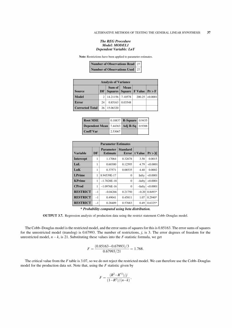
The Cobb–Douglas model is the restricted model, and the error sums of squares for this is 0.85163. The error sums of squares
for the unrestricted model (translog) is 0.67993. The number of restrictions, j, is 3. The error degrees of freedom for the
unrestricted model, n� k, is 21. Substituting these values into the F-statistic formula, we get
F ¼ ð0:85163�0:67993Þ=30:67993=21
¼ 1:768:
The critical value from the F table is 3.07, so we do not reject the restricted model. We can therefore use the Cobb–Douglas
model for the production data set. Note that, using the F statistic given by
F ¼ ðR2�R*2Þ=jð1�R2Þ=ðn�kÞ ;
The REG ProcedureModel: MODEL1
Dependent Variable: LnY
Number of Observations Read 27
Number of Observations Used 27
Analysis of Variance
Source DFSum of
SquaresMean
Square F Value Pr > F
Model 2 14.21156 7.10578 200.25 <0.0001
Error 24 0.85163 0.03548
Corrected Total 26 15.06320
Root MSE 0.18837 R-Square 0.9435
Dependent Mean 7.44363 Adj R-Sq 0.9388
Coeff Var 2.53067
Parameter Estimates
Variable DFParameter
EstimateStandard
Error t Value Pr > |t|
Intercept 1 1.17064 0.32678 3.58 0.0015
LnL 1 0.60300 0.12595 4.79 <0.0001
LnK 1 0.37571 0.08535 4.40 0.0002
LPrime 1 8.94539E-17 0 Infty <0.0001
KPrime 1 –1.7828E-18 0 –Infty <0.0001
CProd 1 –1.0976E-16 0 –Infty <0.0001
RESTRICT –1 –0.04266 0.21750 –0.20 0.8493*
RESTRICT –1 0.49041 0.45811 1.07 0.2940*
RESTRICT –1 0.28409 0.57683 0.49 0.6325*
* Probability computed using beta distribution.
Note: Restrictions have been applied to parameter estimates.
OUTPUT 3.7. Regression analysis of production data using the restrict statement Cobb–Douglas model.
ALTERNATIVE METHODS OF TESTING THE GENERAL LINEAR HYPOTHESIS 37

we get
F ¼ ð0:9549�0:9435Þ=3ð1�0:9549Þ=21 ¼ 1:768;
which is equivalent to the result received when we used the F test with the error sums of squares.
3.5 TESTING FOR STRUCTURAL BREAKS IN DATA
Wecan extend the linear restriction hypothesis test from the previous sections to test for structural breaks in the time periodwithin
which the data setwas collected.We illustrate this by using the gasoline consumption data set given inGreene (2003). The data set
is credited to the Council of Economic Advisors, Washington, D.C. The author gives a description of the model for the gasoline
consumptiondata onpage12of his text. Thedata consists of several variables,which includes the totalU.S. gasoline consumption
(G), computed as total expenditure divided by a price index from 1960 to 1995, the gasoline price index, disposable income, the
price of used and new cars, and so on. A time series plot of G is given in Figure 3.1.
Theplot clearly showsabreak in theU.S. gasoline consumptionbehavior after 1973.Aspointedout inGreene (2003, p.130), up
to 1973, fuel was abundant with stable worldwide gasoline prices. An embargo in 1973 caused a shift marked by shortages and
rising prices.
Consider then a model of the log of per capita gasoline consumption (G/Pop) with respect to the log of the price index of
gasoline (Pg), the logof per capita disposable income (Y), the logof the price indexof newcars (Pnc), and the log of the price index
of used cars (Puc). The regression model is given by (Greene, 2003, p. 136)
lnðG=PopÞ ¼ b1 þb2lnðPgÞþb3lnðyÞþb4lnðPncÞþb5lnðPucÞþ «:
Wewouldexpect that the entire relationship described by this regressionmodelwas shifted starting1974.Let us denote the first
14 years of the data in y and X as y1 and X1 and the remaining years as y2 and X2. An unrestricted regression that allows the
coefficients to be different in the two time periods is given by
y1
y2
� �
¼X1 0
0 X2
� �
b1
b2
� �
þ«1
«2
� �
:
1960 1965 1970 1975 1980 1985 1990 1995
Year
Ln_G_Pop
–0.020.000.020.040.060.080.100.120.140.160.18
–0.04–0.06–0.08–0.10–0.12–0.14–0.16–0.18–0.20–0.22–0.24–0.26–0.28–0.30–0.32–0.34
FIGURE 3.1. Time series plot of total U.S. gasoline consumption from 1960 to 1995.
38 HYPOTHESIS TESTING

The unrestricted least squares estimator is given by (Greene, 2003, pp. 129–130)
b ¼ ðXTXÞ�1XTy ¼ XT
1X1 0
0 XT2X2
" #�1XT
1y1
XT2y2
" #
¼b1
b2
� �
;
which can be obtained by running two regressions separately. If we denote the two residual sums of squares as eT1 e1 and eT2 e2, then
the unrestricted sums of squares is given by eTe ¼ eT1 e1 þ eT2 e2. The restricted least squares estimator can be computed by simply
stacking the data and running least squares regressionon the stackeddata.Let the restricted residual sumsof squares bedenotedby
e*Te*. Then, the hypothesis test on whether the restricted model is more appropriate for the data can be conducted by using the F
statistic discussed earlier. That is,
F ¼ ðe*Te*�eTeÞ=jeTe=ðn1 þ n2�2kÞ :
Note that here j is the number of restrictions (or simply the number of columns ofX2),n1 is the number of observations in the first
data set, and n2 is the number of observations in the second data set. This test is also called the Chow test (Chow, 1960). In the
gasoline consumption example, j¼ 5,n1¼ 14,n2¼ 22, and k¼ 5.Abit later,wewill discuss how toconduct theChow test using the
ProcModel. For now, let us run three regression analyses on the data set. The first two analyses are for the two separate data sets and
the last one is for the combined data set. The output of the analysis on the data set before 1974 is given in Output 3.8. The output of
the analysis for the data set after 1973 is given inOutput 3.9. The output of the analysis of the combined data is given inOutput 3.10.
The REG ProcedureModel: MODEL1
Dependent Variable: Ln_G_Pop
Number of Observations Read 14
Number of Observations Used 14
Analysis of Variance
Source DFSum of
SquaresMean
Square F Value Pr > F
Model 4 0.33047 0.08262 647.56 <0.0001
Error 9 0.00115 0.00012758
Corrected Total 13 0.33162
Root MSE 0.01130 R-Square 0.9965
Dependent Mean –0.13830 Adj R-Sq 0.9950
Coeff Var –8.16742
Parameter Estimates
Variable DFParameter
EstimateStandard
Error t Value Pr > |t|
Intercept 1 –11.32637 1.15233 –9.83 <0.0001
Ln_pg 1 –0.07396 0.16776 –0.44 0.6697
Ln_Income 1 1.25341 0.12914 9.71 <0.0001
Ln_Pnc 1 0.80409 0.12076 6.66 <0.0001
Ln_Puc 1 –0.23754 0.10447 –2.27 0.0491
OUTPUT 3.8. Regression analysis of the gasoline consumption data prior to 1974.
TESTING FOR STRUCTURAL BREAKS IN DATA 39

The sums of squares are as follows: eT1 e1 ¼ 0:00115; eT2 e2 ¼ 0:00792; and e*Te*¼ 0.03384.
Therefore, the Chow test statistic is given by
F ¼ ð0:03384�0:00907Þ=50:00907=26
¼ 14:20:
The p value associated with this is 9.71� 10�7 and is highly significant. We can therefore reject the null hypothesis for the
restricted model and conclude that there is significant evidence that the regression model changed after 1973.
The above computations are unnecessary sinceSASProcModel can be used to test the structural breakhypothesis. ProcModel
is typically used to analyze systems of simultaneous equations and seemingly unrelated regression equationswhere the equations
can be linear or nonlinear. However, it can also be used to conduct basic OLS analysis. Since Proc Reg does not have an option to
conduct the Chow test, we make use of Proc Model.
The following statements can be used to conduct the test. Output 3.11 contains the results of this analysis. Note the threemain
components of the Proc Model statements—the list of parameters (there are 5 in the gasoline consumption model), the actual
model equation being estimated, and the response variable of interest highlighted with the Fit statement. The option “chow=15”
requests a test to determine if the data sets before and after the 15th are significantly different.
proc model data=clean_gas;
parm beta1 beta2 beta3 beta4 beta5;
Ln_G_Pop=beta1 + beta2*Ln_Pg + beta3*Ln_Inc + beta4*Ln_Pnc
The REG ProcedureModel: MODEL1
Dependent Variable: Ln_G_Pop
Number of Observations Read 22
Number of Observations Used 22
Analysis of Variance
Source DFSum of
SquaresMean
Square F Value Pr > F
Model 4 0.05084 0.01271 27.28 <0.0001
Error 17 0.00792 0.00046586
Corrected Total 21 0.05876
Root MSE 0.02158 R-Square 0.8652
Dependent Mean 0.08194 Adj R-Sq 0.8335
Coeff Var 26.34150
Parameter Estimates
Variable DFParameter
EstimateStandard
Error t Value Pr > |t|
Intercept 1 –5.59999 3.00646 –1.86 0.0799
Ln_pg 1 –0.20862 0.04898 –4.26 0.0005
Ln_Income 1 0.63704 0.33190 1.92 0.0719
Ln_Pnc 1 0.06903 0.20662 0.33 0.7424
Ln_Puc 1 –0.02426 0.06311 –0.38 0.7054
OUTPUT 3.9. Regression analysis of the gasoline consumption data after 1973.
40 HYPOTHESIS TESTING

+beta5*Ln_Puc;
Fit Ln_G_Pop/chow=15;
run;
Note that the coefficients in this output are for the restrictedmodel. The p value for the Chow test indicates that themodels are
indeed different between the two time periods.
3.6 THE CUSUM TEST
Model stability can also be tested by using the CUSUM test. See Montgomery (1991), Page (1954), and Woodall and Ncube
(1985) for a discussion of the CUSUM procedure in quality control. See the documentation for Proc Autoreg from the SAS
Institute, Brown et al. (1975), and Greene (2003) for a discussion of the CUSUM procedure to detect structural breaks in the
data. This test is based on the cumulative sum of the least squares residuals. If we let wt ¼ etffiffiffi
vtp (et is the OLS residual at time t)
with
vt ¼ 1þ xTt
X
t�1
i¼1
xixTi
" #�1
xt;
The REG ProcedureModel: MODEL1
Dependent Variable: Ln_G_Pop
Number of Observations Read 36
Number of Observations Used 36
Analysis of Variance
Source DFSum of
SquaresMean
Square F Value Pr > F
Model 4 0.77152 0.19288 176.71 <0.0001
Error 31 0.03384 0.00109
Corrected Total 35 0.80535
Root MSE 0.03304 R-Square 0.9580
Dependent Mean –0.00371 Adj R-Sq 0.9526
Coeff Var –890.84882
Parameter Estimates
Variable DFParameter
EstimateStandard
Error t Value Pr > |t|
Intercept 1 –12.34184 0.67489 –18.29 <0.0001
Ln_pg 1 –0.05910 0.03248 –1.82 0.0786
Ln_Income 1 1.37340 0.07563 18.16 <0.0001
Ln_Pnc 1 –0.12680 0.12699 –1.00 0.3258
Ln_Puc 1 –0.11871 0.08134 –1.46 0.1545
OUTPUT 3.10. Regression analysis of the combined gasoline consumption data.
THE CUSUM TEST 41

The MODEL Procedure
Model Summary
Model Variables 1
Parameters 5
Equations 1
Number of Statements 1
Model Variables Ln_G_Pop
Parameters beta1 beta2 beta3 beta4 beta5
Equations Ln_G_Pop
The Equation to Estimate is
Ln_G_Pop = F(beta1(1), beta2(Ln_pg), beta3(Ln_Income), beta4(Ln_Pnc), beta5(Ln_Puc))
NOTE: At OLS Iteration 1 CONVERGE=0.001 Criteria Met.
The MODEL ProcedureOLS Estimation Summary
Data Set Options
DATA= GASOLINE
Minimization Summary
Parameters Estimated 5
Method Gauss
Iterations 1
Final ConvergenceCriteria
R 2.34E-12
PPC 6.24E-12
RPC(beta1) 122197.4
Object 0.957917
Trace(S) 0.001092
Objective Value 0.00094
ObservationsProcessed
Read 36
Solved 36
OUTPUT 3.11. Chow test of structural break in gasoline data using Proc Model.
42 HYPOTHESIS TESTING

then the CUSUM procedure can be defined as (Baltagi, 2008, p. 191; Greene, 2003, p. 135)
Wt ¼X
r¼t
r¼Kþ 1
;wr
s
where
s2 ¼ ðT�k�1Þ�1X
T
r¼kþ 1
ðwr��wÞ2
and
�w ¼ ðT�kÞ�1X
T
r¼kþ 1
wr:
Here, T and k are the number of time periods and regressors, respectively. The critical values of the CUSUM at time t are
given by
�affiffiffiffiffiffiffiffiffi
T�kp
þ 2ðt�kÞffiffiffiffiffiffiffiffiffi
T�kp
� �
:
Nonlinear OLS Summary of Residual Errors
EquationDF
ModelDF
Error SSE MSE Root MSE R-SquareAdj
R-Sq
Ln_G_Pop 5 31 0.0338 0.00109 0.0330 0.9580 0.9526
Nonlinear OLS Parameter Estimates
Parameter EstimateApproxStd Err t Value
ApproxPr > |t|
beta1 –12.3418 0.6749 –18.29 <0.0001
beta2 –0.0591 0.0325 –1.82 0.0786
beta3 1.373399 0.0756 18.16 <0.0001
beta4 –0.1268 0.1270 –1.00 0.3258
beta5 –0.11871 0.0813 –1.46 0.1545
Number ofObservations Statistics for System
Used 36 Objective 0.000940
Missing 0 Objective*N 0.0338
Structural Change Test
TestBreakPoint Num DF Den DF F Value Pr > F
Chow 15 5 26 14.20 <0.0001
OUTPUT 3.11. (Continued)
THE CUSUM TEST 43
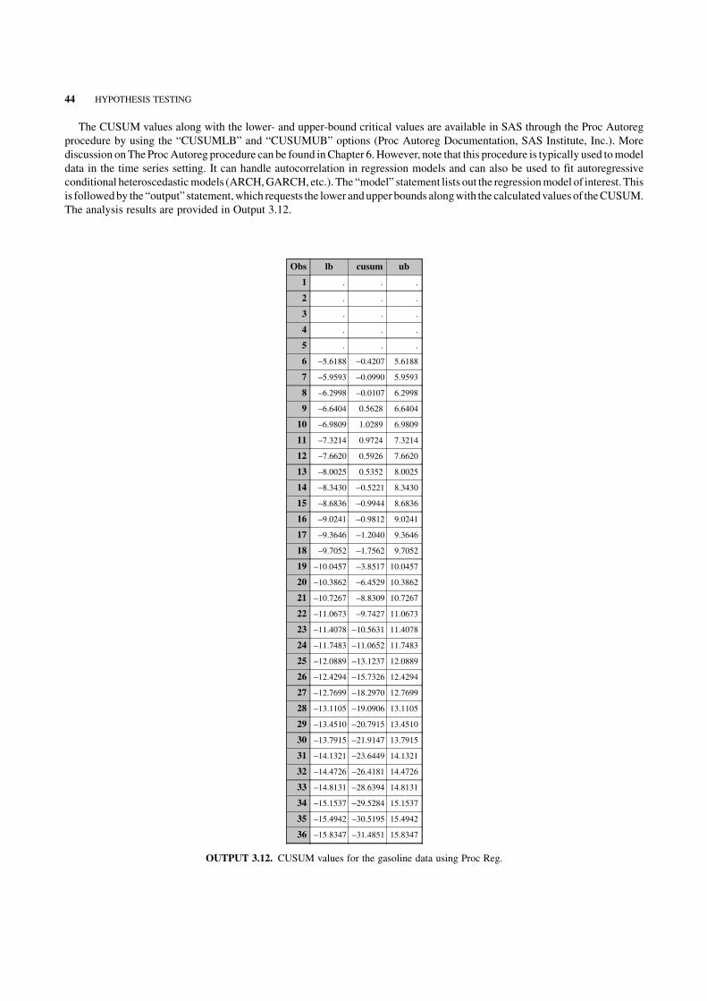
The CUSUM values along with the lower- and upper-bound critical values are available in SAS through the Proc Autoreg
procedure by using the “CUSUMLB” and “CUSUMUB” options (Proc Autoreg Documentation, SAS Institute, Inc.). More
discussion onThe ProcAutoreg procedure can be found inChapter 6.However, note that this procedure is typically used tomodel
data in the time series setting. It can handle autocorrelation in regression models and can also be used to fit autoregressive
conditional heteroscedasticmodels (ARCH,GARCH, etc.). The “model” statement lists out the regressionmodel of interest. This
is followedby the “output” statement,which requests the lower andupper bounds alongwith the calculatedvalues of theCUSUM.
The analysis results are provided in Output 3.12.
Obs lb cusum ub
1 . . .
2 . . .
3 . . .
4 . . .
5 . . .
6 –5.6188 –0.4207 5.6188
7 –5.9593 –0.0990 5.9593
8 –6.2998 –0.0107 6.2998
9 –6.6404 0.5628 6.6404
10 –6.9809 1.0289 6.9809
11 –7.3214 0.9724 7.3214
12 –7.6620 0.5926 7.6620
13 –8.0025 0.5352 8.0025
14 –8.3430 –0.5221 8.3430
15 –8.6836 –0.9944 8.6836
16 –9.0241 –0.9812 9.0241
17 –9.3646 –1.2040 9.3646
18 –9.7052 –1.7562 9.7052
19 –10.0457 –3.8517 10.0457
20 –10.3862 –6.4529 10.3862
21 –10.7267 –8.8309 10.7267
22 –11.0673 –9.7427 11.0673
23 –11.4078 –10.5631 11.4078
24 –11.7483 –11.0652 11.7483
25 –12.0889 –13.1237 12.0889
26 –12.4294 –15.7326 12.4294
27 –12.7699 –18.2970 12.7699
28 –13.1105 –19.0906 13.1105
29 –13.4510 –20.7915 13.4510
30 –13.7915 –21.9147 13.7915
31 –14.1321 –23.6449 14.1321
32 –14.4726 –26.4181 14.4726
33 –14.8131 –28.6394 14.8131
34 –15.1537 –29.5284 15.1537
35 –15.4942 –30.5195 15.4942
36 –15.8347 –31.4851 15.8347
OUTPUT 3.12. CUSUM values for the gasoline data using Proc Reg.
44 HYPOTHESIS TESTING

proc autoreg data=gasoline noprint;
model Ln_G_Pop=Ln_Pg Ln_Income Ln_Pnc Ln_Puc;
output out=cusum cusum=cusum cusumub=ub cusumlb=lb;
run;
proc print data=cusum;
var lb cusum ub;
run;
The CUSUM plot can be created using the overlay option of Proc Gplot. The following statements are used. The results are
provided in Figure 3.2.
proc gplot data=cusum;
title ’The CUSUM Test on Gasoline Consumption Data’;
plot lb*year cusum*year ub*year/overlay;
run;
Note that a structural break is obvious around 1984. This is a bit contradictory to the results obtained fromChow’s test, where
the structural break was evident at 1974. However, there is evidence that the structural break started occurring around 1974.
3.7 MODELS WITH DUMMY VARIABLES
The models discussed so far consisted of quantitative explanatory variables. Often, the models of interest have explanatory
variables that are discrete. A simple example is a variable recording the gender of a subject. Here gender may be set to 1 if the
subject is amale and 0 if the subject is a female.As another example, consider a transportation studywhere one of the explanatory
variables records the mode of public transportation used by the subjects in the study. Here, the values of the variable may be
classified into three categories: Drive own car, Take Bus, and Take Metro. Practitioners familiar with Analysis of Variance
(ANOVA) techniquesmay recall that this is analogous to thedifferent levelsofa treatment of interest.Here, the treatment is simply
themode of transportation. Greene (2003, p.116) discusses an examplewhere the earning�s of women ismodeled as a function of
lb
-40
-30
-20
-10
0
10
20
Year
1960 1970 1980 1990 2000
FIGURE 3.2. The CUSUM test on gasoline consumption data.
MODELS WITH DUMMY VARIABLES 45

age, a squared age term, level of education, and the presence or absenceof childrenunder 18.The data are credited toMroz (1987).
The model of interest is
lnðearningsÞ ¼ b1 þb2 � ageþb3 � age2 þb4 � educationþb5 � kidsþ «:Here,
kids ¼ 1 if there are kids < 18;
0 otherwise
�
No special treatment is required in this case, and estimating the coefficients is straightforward using the techniques discussed
so far. The analysis results are shown in Output 3.13. The estimated model for In(earnings) is given by
lnðearningsÞ ¼ 3:24 þ 0:20� age � 0:0023� age2 þ 0:067� education � 0:35� kids:
The earnings equation for women without children under 18 is given by
lnðearningsÞ ¼ 3:24þ 0:20� age � 0:0023� age2 þ 0:067� education
and the earnings equation for women with children under 18 is given by
lnðearningsÞ ¼ 2:89þ 0:20� age � 0:0023� age2 þ 0:067� education:
The REG ProcedureModel: MODEL1
Dependent Variable: L_WW
Number of Observations Read 428
Number of Observations Used 428
Analysis of Variance
Source DFSum of
SquaresMean
Square F Value Pr > F
Model 4 25.62546 6.40637 4.52 0.0014
Error 423 599.45817 1.41716
Corrected Total 427 625.08363
Root MSE 1.19044 R-Square 0.0410
Dependent Mean 8.05713 Adj R-Sq 0.0319
Coeff Var 14.77504
Parameter Estimates
Variable Label DFParameter
EstimateStandard
Error t Value Pr > |t|
Intercept Intercept 1 3.24010 1.76743 1.83 0.0675
WA WA 1 0.20056 0.08386 2.39 0.0172
WA_SQ 1 –0.00231 0.00098688 –2.35 0.0195
WE WE 1 0.06747 0.02525 2.67 0.0078
kids 1 –0.35120 0.14753 –2.38 0.0177
OUTPUT 3.13. Regression analysis of earnings data using Proc Reg.
46 HYPOTHESIS TESTING

Notice that the earningsmodel is a semi-logmodel (log in thedependent variable).Wecan therefore interpret the coefficient for
the dummy variable kids as follows: ceteris paribus, the earnings of womenwith children under 18 are 35% less than the earnings
of women without children under 18.
The general rule for creating dummy variables is to have one less variable than the number of categories present to avoid the
“dummy variable trap”. If a dummy variable category is not removed then the sum of the dummy variable category columns will
equal “1”which will result in perfect multicollinearity in models with a constant term. Recall that the data matrixX for a model
with an intercept term includes a column of 1�s.
The earning�s equation model had one dummy variable since we were dealing with two categories (kids under 18 or not).
Suppose thatwewanted to compare threegroups: onewith children under 10, anotherwith children between the ages of 10 and18,
and a third group of children above 18. In this case we would need to include two dummy variables. Suppose the variables were
labeled Age_Grp1 and Age_Grp2. Here,
Age ---- Grp1¼1 if age <10
0 otherwise
(
Age ---- Grp2¼1 if 10 � age <18
0 otherwise:
(
The thirdgroupwith childrenabove theageof18 forms the“base”.Of course, the coding schemecanbeadjusted tomakeanyof
the groups the “base”.
Wewill now look at a detailed example to illustrate the concept of dummy variables. Consider the airline data set in Greene
(2003). Six airlines were followed for 15 years, and the following consumption model was proposed for the data set (Greene,
2003, pp. 118–119)
lnðCi;tÞ ¼ b1 þb2lnðQi;tÞþb3ln2ðQi;tÞþb3lnðPfuel i;tÞþb5Loadfactori;t þ
X
14
t¼1
�tDi;t þX
5
i¼1
diFi;t þ «i;t:
The data set is credited to Christensen Associates of Madison, Wisconsin. The author provides a description of the data and
model which is summarized here. In this model, the subscript i refers to airline, and the subscript t refers to year. The variableCi,t
represents the total cost (in 1000�s) for the ith firm in the tth year,Q is the output in revenue passenger miles, PF is the fuel price,
and LF is the load factor or the average capacity utilization of the fleet. Note that the year 1984 is kept as a base, and we have 14
dummyvariables for year. Similarly, oneof the firms (Firmnumber 6)waskept as a base andwe therefore have5dummyvariables
for firm.Wewill look at how the data are prepared for analysis in Proc IML and Proc Reg and thenmove on to analysis using Proc
GLM. The following data statement will create the dummy variables. The array statement provides a convenient way of creating
indicator variables for the six airlines and 14 time periods.
data airline;
set airline;
LnC=Log(C);
LnQ=Log(Q);
LnQ2=LnQ*LnQ;
LnPF=Log(PF);
array Firm{*} F1-F5;
array time_y{*} D1-D14;
do index1=1 to dim(Firm);
if index1=i then Firm(index1)=1;else Firm(index1)=0;
end;
do index2=1 to dim(time_y);
if index2=t then time_Y(index2)=1;else time_Y(index2)=0;
end;
run;
The data can now be analyzed in Proc IML easily using the code provided in Chapter 2. Of course, an easier approach is to
analyze the data using Proc Reg. The output of the analysis from Proc Reg is given in Output 3.14.
MODELS WITH DUMMY VARIABLES 47

The REG ProcedureModel: MODEL1
Dependent Variable: LnC
Number of Observations Read 90
Number of Observations Used 90
Analysis of Variance
Source DFSum of
SquaresMean
Square F Value Pr > F
Model 23 113.86832 4.95080 1893.45 <0.0001
Error 66 0.17257 0.00261
Corrected Total 89 114.04089
Root MSE 0.05113 R-Square 0.9985
Dependent Mean 13.36561 Adj R-Sq 0.9980
Coeff Var 0.38258
Parameter Estimates
Variable Label DFParameter
EstimateStandard
Error t Value Pr > |t|
Intercept Intercept 1 13.56249 2.26077 6.00 <0.0001
LnQ 1 0.88665 0.06284 14.11 <0.0001
LnQ2 1 0.01261 0.00986 1.28 0.2053
LnPF 1 0.12808 0.16576 0.77 0.4425
LF LF 1 –0.88548 0.26051 –3.40 0.0012
D1 1 –0.73505 0.33784 –2.18 0.0332
D2 1 –0.67977 0.33209 –2.05 0.0447
D3 1 –0.64148 0.32983 –1.94 0.0561
D4 1 –0.58924 0.31954 –1.84 0.0697
D5 1 –0.49925 0.23176 –2.15 0.0349
D6 1 –0.44304 0.18796 –2.36 0.0214
D7 1 –0.41131 0.17290 –2.38 0.0203
D8 1 –0.35236 0.14972 –2.35 0.0216
D9 1 –0.28706 0.13470 –2.13 0.0368
D10 1 –0.23280 0.07611 –3.06 0.0032
D11 1 –0.09678 0.03385 –2.86 0.0057
D12 1 –0.01227 0.04585 –0.27 0.7899
D13 1 –0.00187 0.03816 –0.05 0.9611
D14 1 –0.01296 0.03069 –0.42 0.6742
Parameter Estimates
Variable Label DFParameter
EstimateStandard
Error t Value Pr > |t|
F1 1 0.05930 0.12421 0.48 0.6346
F2 1 0.02214 0.10438 0.21 0.8327
F3 1 –0.18000 0.05900 –3.05 0.0033
F4 1 0.16856 0.03326 5.07 <0.0001
F5 1 –0.04543 0.02238 –2.03 0.0464
OUTPUT 3.14. Dummy variables regression of the airlines data.
48 HYPOTHESIS TESTING

We will now analyze the data using Proc GLM. Note that in this case, we do not have to create dummy variables as the
procedures automatically creates them for us. ProcGLMcanbeused to fit general linearmodels using themethod of least squares.
It can therefore be used for regression analysis, analysis of variance, and analysis of covariance. An advantage of Proc GLMover
Proc Reg is that one can incorporate interaction terms directly into themodel. Of course, one can also analyze nested and crossed
effects designs very easily within Proc GLM. It also provides the flexibility of analyzing random and fixed effects in the model.
The procedure also provides an overall significance of the classificationvariables that quickly helps the analyst gaugewhether the
variables are significant or not. In the following statements, the “class” statement is used to specify category variables. This is
followedby the “model” statement that lists out the dependent variable and the explanatory variables in themodel. The “solution”
option in the “model” statement generates the parameter estimates for all the terms in the model.
The following statements should be used at the minimum.
proc glm data=airline;
class I T;
model LnC=LnQ LnQ2 LnPF LnLF I T/solution;
run;
The output from the analysis is given inOutput 3.15. The first set of tables gives information on the classificationvariables and
the sample size used in the analysis. In thegasoline example,wehave six airlines and15 timeperiods for a total of 90observations.
The next table gives the analysis of variance table which lists out the sources of variation, the degrees of freedom, the sums of
squares, themean squares, theF statistic, and thecorrespondingpvalues.Note that the total degreesof freedom is90�1¼89.The
The GLM Procedure
Class Level Information
Class Levels Values
I 6 1 2 3 4 5 6
T 15 1 2 3 4 5 6 7 8 9 10 11 12 13 14 15
Number of Observations Read 90
Number of Observations Used 90
The GLM Procedure
Dependent Variable: LnC
Source DFSum of
Squares Mean Square F Value Pr > F
Model 23 113.8683247 4.9507967 1893.45 <0.0001
Error 66 0.1725702 0.0026147
Corrected Total 89 114.0408949
R-Square Coeff Var Root MSE LnC Mean
0.998487 0.382580 0.051134 13.36561
Source DF Type I SS Mean Square F Value Pr > F
LnQ 1 103.6813479 103.6813479 39653.2 <0.0001
LnQ2 1 0.0618892 0.0618892 23.67 <0.0001
LnPF 1 8.7201792 8.7201792 3335.06 <0.0001
LF 1 0.3025573 0.3025573 115.71 <0.0001
I 5 1.0067672 0.2013534 77.01 <0.0001
T 14 0.0955840 0.0068274 2.61 0.0046
OUTPUT 3.15. Dummy variable regression of airlines data using Proc GLM.
MODELS WITH DUMMY VARIABLES 49

model degrees of freedom is calculated as follows: one degree of freedom is used for each explanatory variable in the model and
a�1 degrees of freedom are used for the classification variables where a is the number of levels of the classification variable. For
the airlines example, we have four explanatory variables that contribute one degree of freedom, the six airlines contribute
5 degrees of freedom, and the 15 time periods contribute 14 degrees of freedom. Therefore, the total model degrees of freedom
equals 24. Note that the p value indicates that the “global” F test for model significance is rejected.
Source DF Type III SS Mean Square F Value Pr > F
LnQ 1 0.52059518 0.52059518 199.10 <0.0001
LnQ2 1 0.00427810 0.00427810 1.64 0.2053
LnPF 1 0.00156096 0.00156096 0.60 0.4425
LF 1 0.03020843 0.03020843 11.55 0.0012
I 5 0.86213348 0.17242670 65.95 <0.0001
T 14 0.09558402 0.00682743 2.61 0.0046
Parameter EstimateStandard
Error t Value Pr > |t|
Intercept 13.56249268 B 2.26076834 6.00 <0.0001
LnQ 0.88664650 0.06283642 14.11 <0.0001
LnQ2 0.01261288 0.00986052 1.28 0.2053
LnPF 0.12807832 0.16576427 0.77 0.4425
LF –0.88548260 0.26051152 –3.40 0.0012
I 1 0.05930014 B 0.12420645 0.48 0.6346
I 2 0.02213860 B 0.10437912 0.21 0.8327
I 3 –0.17999872 B 0.05900231 –3.05 0.0033
I 4 0.16855825 B 0.03326401 5.07 <0.0001
Parameter EstimateStandard
Error t Value Pr > |t|
I 5 –0.04543271 B 0.02238459 –2.03 0.0464
I 6 0.00000000 B . . .
T 1 –0.73505414 B 0.33783895 –2.18 0.0332
T 2 –0.67976508 B 0.33209031 –2.05 0.0447
T 3 –0.64147600 B 0.32983272 –1.94 0.0561
T 4 –0.58924090 B 0.31953812 –1.84 0.0697
T 5 –0.49924839 B 0.23175982 –2.15 0.0349
T 6 –0.44304017 B 0.18795980 –2.36 0.0214
T 7 –0.41130701 B 0.17289580 –2.38 0.0203
T 8 –0.35235703 B 0.14971845 –2.35 0.0216
T 9 –0.28705848 B 0.13470473 –2.13 0.0368
T 10 –0.23279711 B 0.07610725 –3.06 0.0032
T 11 –0.09678442 B 0.03385162 –2.86 0.0057
T 12 –0.01226693 B 0.04585181 –0.27 0.7899
T 13 –0.00186796 B 0.03815702 –0.05 0.9611
T 14 –0.01295665 B 0.03068805 –0.42 0.6742
T 15 0.00000000 B . . .
Note: The X'X matrix has been found to be singular, and a generalized inverse was used to solve the normal equations. Terms whose estimates are followed by the letter 'B' are not uniquely estimable.
OUTPUT 3.15. (Continued )
50 HYPOTHESIS TESTING

This is followed by the R2 value, the coefficient of variation (see Chapter 2), the root mean square error, and the mean of the
dependent variable. Notice that the R2 value is very high.
The next two tables gives the Type 1 and Type 3 sums of squares for each term in the model along with their F statistic and
p values. The Type 1 sums of squares gives the amount of variation attributed to each term in the model assuming that the terms
listed in the table before it has already been included in the model. This is also referred to as the sequential sums of squares. The
Type 3 sums of squares gives the amount of variation attributed to each term after adjusting for the other terms. In other words, it
measures the amount bywhich the error sumsof squares is reduced if the term in question is added to amodel already consisting of
the other terms. Note that the p values for the four explanatory variables from the Type 3 sums of squares matches the p values of
the variables fromProc Reg. Proc Reg uses Type 3 sums of squares since our objective is to determine if the variable in question is
meaningful to the generalmodel consisting of the other terms. The p values from theType 3 table indicates that the load factor, the
airlines, and the time periods are significantly different.
The “solution” option is used to list out the parameter estimates. Note that the coefficients are identical to the ones from Proc
Regwhere dummy variables were used. Also notice that the sixth airline and the 15th time period have been taken as a base. The
interpretationof themodels for the other firmswill be relative to the sixth firm.Note that firms3, 4, and5are significantly different
from firm 6. Also note that the first 11 time periods are significantly different from the 15th time period.
MODELS WITH DUMMY VARIABLES 51

4INSTRUMENTALVARIABLES
4.1 INTRODUCTION
The analysis methods presented in the previous chapters were based on the assumption that the independent variables are
exogenous (E(e jX)¼ 0). That is, the error terms in the linear regressionmodel are uncorrelated or independent of the explanatory
variables. In Chapter 1, we saw that under the exogeneity assumption, the least squares estimator b is an unbiased and consistent
estimator of b. This chapter explores the properties of b under departures from the exogenous assumption? Explanatory variables
that are not exogenous are called endogenous variables.
Under departures from the exogeneity conditions, b is no longer an unbiased and consistent estimator of b. To see this, in the
simple linear regression case, consider the model yi¼b0 þ b1xiþ «iwhere the disturbances are correlated with the explanatory
variable. The least squares estimator of b1 is given by (Chapter 1)
b1¼
P
n
i¼1
ðxi� x�Þðyi� y�Þ
P
n
i¼1
ðxi� x�Þ2
which upon simplifying can be written as
b1¼ b1þ
P
n
i¼1
ðxi� x�Þð«i� «�Þ
P
n
i¼1
ðxi� x�Þ2:
The second termgives the expressionof the least squares estimator of a regressionof«on x. It should beobvious that the second
term is not zero unless the disturbances are uncorrelatedwith the explanatory variable. Therefore, the least squares estimator ofb1
is biased. The inconsistency of the least squares estimator can be seen by dividing the numerator and denominator of the second
term by n and then taking the probability limits to get
p lim b1ð Þ ¼ b1þCovð«; xÞ
VarðxÞ:
52
Applied Econometrics Using the SAS� System, by Vivek B. AjmaniCopyright � 2009 John Wiley & Sons, Inc.

The least squares estimator is therefore not consistent. Themagnitude and direction of the bias depend on the second term of
the above expression.
To see this in the general case, consider the linear model y ¼ Xbþ e with EðejXÞ ¼ g. The OLS estimator is given by
b ¼ ðXTXÞ�1XTy or b ¼ bþ ðXTXÞ�1
XTe. Taking the conditional expectation EðbjXÞ, we see that (Greene, 2003, p. 76)
EðbjXÞ ¼ bþ ðXTXÞ�1EðXT
ejXÞ
¼ bþ ðXTXÞ�1XTEðejXÞ
¼ bþ ðXTXÞ�1g 6¼ b :
Next, assume that p lim ðXTX=nÞ ¼ C a positive definite matrix with inverse C�1. Note that this assumption ensures that
ðXTXÞ�1exists (in the simple linear regression case, this assumption implied thatVarðxÞ existed andwas finite). Taking the limit
in the probability of OLS estimator, we get
p lim b ¼ bþC�1p lim
XTe
n
� �
6¼ b
because E (e | X) 6¼ 0. Therefore, the OLS estimator is not a consistent estimator if the exogeneity assumption is violated.
Endogeneity occurs for several reasons. Missing variables andmeasurement errors in the independent variables are often cited
as major causes of endogeneity in regression models (Ashenfelter et al., 2003; Greene, 2003; Wooldridge, 2002). We will now
briefly discuss both the omitted variable bias and the bias emerging from measurement errors.
4.2 OMITTED VARIABLE BIAS
The analysis in Chapters 1 through 3 was also based on the assumption that the linear model y¼Xb þ e was correctly
specified.Wewill now relax this assumption and see the effect this has on the parameter estimates. Suppose that X¼ [X1,X2]
and b¼ [b1, b2]T so that the true model is y¼X1b1 þ X2b2 þ e. Assume that for some reason we have no information
available forX2 and therefore omit it and fit the model y¼X1b1 þ e. The least squares estimator of b1 in this case is given by
(Greene, 2003, p. 148)
b1 ¼ ðXT1X1Þ
�1XT
1y
¼ b1 þ ðXT1X1Þ
�1XT
1X2b2 þ ðXT1X2Þ
�1XT
1 e:
It is easy to verify that the conditional expectation of b1 given X is
Eðb1jXÞ ¼ b1 þ ðXT1X1Þ
�1XT
1X2b2:
The bias is given by the second termand is zero only ifXT1X2 ¼ 0 (X1 andX2 are orthogonal). That is, if the omitted variables
are not correlated with the included variables. Under the omitted variable model, the termX2b2 is absorbed into the error term.
If the omitted variableX2 is related toX1, then it can easily be shown thatCovðejXÞ6¼ 0 and therefore the exogenous assumption
is violated.
To see this, consider the simple linear model given by y ¼ b0 þ b1x1 þ b2x2 þ « and assume that this is the true population
model. Consider the case where x2 is omitted so that the model used is y ¼ b0 þ b1x1 þ «. Assume that x2 is correlated with x1with the reduced form for x2 given by x2 ¼ a0 þ a1x1 þ �. As shown earlier, the OLS estimator of b1 is given by
b1 ¼
P
n
i¼1
ðx1i�x�1Þðyi� y�Þ
P
n
i¼1
ðx1i�x�1Þ2
:
OMITTED VARIABLE BIAS 53

Substituting the true populationmodel in the above expression and after some elementary algebraicmanipulations, it can be
shown that
b1 ¼ b1 þ b2
P
n
i¼1
ðx1i�x�1Þðx2i�x�2Þ
P
n
i¼1
ðx1i�x�1Þ2
þ
P
n
i¼1
ðx1i�x�1Þð«i� «�Þ
P
n
i¼1
ðx1i�x�1Þ2
:
The last term in the conditional expectation Eðb1jx1i; x2iÞ drops out giving
b1 ¼ b1 þ b2
P
n
i¼1
ðx1i�x�1Þðx2i�x�2Þ
P
n
i¼1
ðx1i�x�1Þ2
:
Again, the second term gives the least squares estimator of a regression of x2 on x1. It should be obvious that the OLS
estimator of b1 is biased unless Covðx1; x2Þ ¼ 0 with the magnitude and direction of the bias depending on the second term of
the above expression.
4.3 MEASUREMENT ERRORS
Wewill now look at howmeasurement errors in the explanatory or dependent variables or both affect the least squares estimators.
It turns out that the measurement error in the explanatory variables creates a correlation between the variables and the error term
similar to the omitted variable case. On the other hand, measurement errors in the dependent variable may not be a problem
(Wooldridge, 2002).Wewill illustrate the issue byusing a simple linear regressionmodelwith just one explanatoryvariable—that
is, a model of the form (Ashenfelter et al., 2003, p. 197):
yi ¼ b0 þ b1xi þ «i i ¼ 1; . . . ; n
where xi is assumed to be exogenous. Suppose that we observe xi with error. That is, we observe x0i ¼ xi þ ui. Assume that x is
independent of ui and that the disturbances ui and «i are independent of each other. Furthermore, assume that ui � i:i:d:ð0;s2uÞ and
«i � i:i:d:ð0;s2«Þ.
By substituting the observed value x0i in the equation for yi, we get yi ¼ b0 þ b1x0i þ �i where �i ¼ «i�b1ui. Note that by
constructionCovð�i; x0iÞ 6¼ 0 since both x0i and �i are influenced by the random component ui. Therefore, the OLS assumptions
are violated and the least squares estimate forb1 is biased and inconsistent. To see this, note that theOLS estimate forb1 can be
written as
b1 ¼
P
n
i¼1
ðx0i�x�0Þðyi� y�Þ
P
n
i¼1
ðx0i�x�0Þ2
:
Simple algebraic manipulation can be used to rewrite the above expression as
b1 ¼ b1 þ
P
n
i¼1
ðx0i�x�0Þð�i� ��Þ
P
n
i¼1
ðx0i�x�0Þ2
:
Dividing the numerator and denominator of the second term by n and taking the probability limits gives
b1 ¼ b1 þCovðx0; �Þ
Varðx0Þ:
54 INSTRUMENTALVARIABLES

Using the assumptions stated earlier, it can be easily shown thatCovðx0; �Þ ¼ �b1s2u and thatVarðx
0Þ ¼ s2x þ s2
u. Therefore,
the bias is given by
�b1s
2u
s2x0 þ s2
u
:
Therefore, measurement errors in the explanatory variables result in biased and inconsistent OLS estimates. As before, the
magnitude and the direction of the bias depend on the second term of the expression of b1.
Ashenfelter et al. (2003, p. 197) gives an elegant derivation to show the behavior of the least squares estimator under
measurement errors in both the dependent and the independent variables. As discussed by the authors, measurement errors in the
dependent variable, in general, does not lead to violation of the least squares assumptions because the measurement error in
the dependent variable is simply absorbed in the disturbance term of the model. However, errors in the dependent variable may
inflate the standard errors of the least squares estimates. To see this, consider the simple linear regressionmodel given earlier and
assume thatwedonot observeyibut observey0i ¼ yi þ vi. Substituting this in theoriginalmodel,wegety0i ¼ b0 þ b1xi þ uiwhere
ui ¼ «i þ vi. It should be obvious that unlessCovðxi; viÞ 6¼ 0, theOLS assumptions are not violated. Furthermore, since (Meyers,
1990, p. 14)
Var b1
� �
¼s2u
P
n
i¼1
ðxi� x�Þ2;s2
u ¼ s2« þ s2
v ; ands2x ¼ n�1
X
n
i¼1
ðxi� x�Þ2
then
Var b1
� �
¼s2« þ s2
u
ns2x
:
Therefore, the measurement errors in the dependent variable tends to inflate the standard errors of the estimates.
4.4 INSTRUMENTALVARIABLE ESTIMATION
Wewill now discuss an alternative method to get unbiased and consistent estimators of b under departures from the exogenous
assumption. To motivate the discussion of instrumental variables, consider the least squares model given by
y ¼ XTb þ e:
Assume that one ormore variables inXmay be correlatedwith e. That is, assume thatE(ejX)¼h 6¼ 0. Next, assume that there
exists a set ofLvariables inW,withL � k, such thatCovðW;XÞ 6¼ 0butEðWTeÞ ¼ 0. That is, theLvariables inWare exogenous
but are correlated with the explanatory variables. Check this.
Note that the exogenousvariables from theoriginal set of variablesmaybepart ofW. Thevariables in the setWare referred to as
instrumental variables.Wewill first look at the instrumental variable estimator for the casewhenL ¼ k. Premultiplying the linear
model by WT gives
WTy ¼ WTXbþWTe:
By rewriting this as
y* ¼ X*bþ e*
and using the method of least squares, we can write
bIV ¼ ðX*TX*Þ�1X*Ty* ¼ ðXTWWTXÞ�1
XTWWTy;
INSTRUMENTALVARIABLE ESTIMATION 55

which can be simplified to
bIV ¼ bþ ðWTXÞ�1WT
e :
Using the assumption that ðWTXÞ�1exists andEðWT
eÞ ¼ 0, it is easy to show that bIV is unbiased forb. Using the discussion
used to show the consistency of OLS estimators, it is trivial to show that p lim ðbIVÞ ¼ b.Therefore, the instrumental variable estimator for the case L ¼ k is
bIV ¼ ðXTWWTXÞ�1XTWWT ;
which can be simplified to
bIV ¼ ðWTXÞ�1WTy:
Greene (2003, pp. 76–77) gives a thorough description and the assumptions underlying the instrumental variables estimator.
Also see Wooldridge (2002, pp. 85–86) and Ashenfelter et al. (2003, pp. 199–200).
It is easy to show that the asymptotic variance of bIV is
s 2ðWTXÞ�1ðWTWÞðXTWÞ�1
where,
s2 ¼ðy�XbIVÞ
Tðy�XbIVÞ
nðGreene; 2003; p: 77Þ:
.
As shown in Greene (2003, p. 78 andWooldridge (2002, pp. 90–91), instrumental variables estimation when L > k is done in
two steps. In Step 1, the data matrix X is regressed against the matrix containing the instrumental variablesW to get Xwhich is
defined as X¼ ðWTWÞ�1WTX. In Step 2, y is regressed on X to get the instrumental variables estimator, bIV given by
bIV ¼ðXT XÞ�1XTy
¼ ½XTWðWTWÞ�1WTX��1XTWðWTWÞ�1WTy:
This estimator is often referred to as the two-stage least squares estimator of b and is abbreviated as 2SLS. The k� kmatrix
s2ðXT XÞ�1with
s2 ¼ðy� XbIVÞ
Tðy� XbIVÞ
n
is the estimated covariance matrix of the 2SLS estimator.
We will now illustrate the computations involved in estimation with instrumental variables by using the data on working,
marriedwomen in thewell-known labor supply data fromMroz (1987).As discussed inWooldridge (2002, p. 87), the objective is
to estimate the following wage equation:
logðwageÞ ¼ b0 þ b1exper þ b2exper2 þ b3educ þ «:
The variable educ contains the actual number of years of education of each woman. As stated by the author, information on
ability of the women, the quality of education received and their family background is missing. These variables are suspected of
being correlated with the education variable and are therefore assumed to contribute to omitted variables bias. Suppose that
information on mother’s education, motheduc, is available so that it can be used as an instrument for educ. The instrumental
variables matrix W therefore has three variables: exper, exper2, and motheduc.
56 INSTRUMENTALVARIABLES

Wewill first analyze the data in Proc IML and then show the analysis in Proc Syslin. The following statements will read in the
data from a text file called “mroz_raw.txt.” Note that the variable inlf indicates whether a person was in the labor force in 1975.
Since we are interested in working women, we need to select only those records where inlf¼ 1.
data mroz;
infile ’C:\Temp\MROZ.txt’ lrecl=234;
input inlf hours kidslt6 kidsge6 age educ wage repwage
hushrs husage huseduc huswage faminc mtr motheduc
fatheduc unem city exper nwifeinc lwage expersq;
if inlf=1;
run;
Next, we read the data into matrices by using Proc IML. Note that the data matrix X has data for the actual labor market
experience (exper), the squared term for this (exper2), and years of schooling (educ). Of course, we need to also add the constant
column of 1’s. The response variable is the log of wage (log(wage)). We use the mother’s years of schooling (motheduc) as the
instrument for educ. Therefore, the instrumental variables matrix W contains the column of 1’s along with exper, exper2, and
motheduc. The following statements invoke Proc IML and read the data into the matrices.
Proc IML;
use mroz;
read all var {’exper’ ’expersq’ ’educ’} into X;
read all var {’lwage’} into Y;
read all var {’exper’ ’expersq’ ’motheduc’} into W;
n=nrow(X);
k=ncol(X);
X=J(n,1,1)||X;
W=J(n,1,1)||W;
As discussed earlier, when the number of columns of W equals the number of columns of X, the least squares instrumental
variables estimator is given by bIV¼ (WTX)�1WTy. The following statement will calculate this.
bhat_IV=inv(W’*X)*W’*y;
We can calculate the asymptotic variance–covariance matrix of this estimator by using the formulas outlined in this section.
The following statements can be used to calculate the standard errors of the instrumental variable estimator. Output 4.1 contains
the analysis results.
variance=((y-X*bhat_IV)’*(y-X*bhat_IV)/n;
variance_matrix=inv(W’*X)*(W’*W)*inv(X’*W);
var_cov_IV=variance*variance_matrix;
SE=SQRT(vecdiag(var_cov_IV));
Themodel used is a semi-logmodel and can be interpreted as follows: Ceteris Paribus, the estimate of the return to education is
about 5% and is not significant. The implication is that each additional year of school is predicted to increase earnings by about
TABLE
BHAT_IV SE T PROBT
INTERCEPT 0.1982 0.4707 0.4211 0.6739
EXPER 0.0449 0.0135 3.3194 0.0010
EXPER_SQ –0.0009 0.0004 –2.2797 0.0231
EDUC 0.0493 0.0373 1.3221 0.1868
OUTPUT 4.1. Instrumental variable estimates for the earning data.
INSTRUMENTALVARIABLE ESTIMATION 57

5%.The estimate of return to schooling fromOLSestimation is about 10.7%and is highly significant. The standard error from the
instrumental variable estimation is 0.0373versus0.014 for theOLSmodel. The t-test value for the instrumental variable estimator
is therefore smaller than that from the OLS estimation, which explains the difference between the lack of significance of the
instrumental variables estimator to the OLS estimator. The OLS model is given in Output 4.3.
The Proc Syslin procedure in SAS can be used to conduct instrumental variable analysis on the earning data. This procedure is
extremely powerful and can be used to estimate parameters in systems of seemingly unrelated regression and systems of
simultaneous equations. It can also be used for single equation estimation using OLS and is very useful when conducting
instrumental variables regression for both the single andmultiple equations systems. The following statements can be used at the
minimumfor instrumental variables analysis of the earningdata.Note that allwedohere is specify the endogenous and exogenous
variables followed by a specification of the linear model. The analysis results are given in Output 4.2.
proc syslin 2SLS data=mroz;
endogenous educ;
instruments exper expersq motheduc;
model lwage=exper expersq educ;
run;
The t-tests indicate that both experience variables are significant. The output from Proc Syslin (using the options for the
example used) is very similar to the outputwe have seenwith ProcReg andProcGLM.That is, weget theANOVA table, followed
by the model statistics and the parameter estimates. The results from OLS analysis are given in Output 4.3 and indicates a
significance of all three variables.
We now turn our attention to the casewhen the number of columns inWexceeds the number of columns inX.Wewill now use
the informationonboth parents’ education (fatheduc and motheduc) and husband’s education (huseduc) as instruments foreduc.
As before, we will analyze this data using Proc IML followed by analysis using Proc Syslin.
Model lwage
Dependent Variable lwage
Analysis of Variance
Source DFSum of
SquaresMean
Square F Value Pr > F
Model 3 10.18121 3.393735 7.35 <0.0001
Error 424 195.8291 0.461861
Corrected Total 427 223.3275
Root MSE 0.67960 R-Square 0.04942
Dependent Mean 1.19017 Adj R-Sq 0.04270
Coeff Var 57.10123
Parameter Estimates
Variable DFParameter
EstimateStandard
Error t Value Pr > |t|
Intercept 1 0.198186 0.472877 0.42 0.6754
exper 1 0.044856 0.013577 3.30 0.0010
expersq 1 –0.00092 0.000406 –2.27 0.0238
educ 1 0.049263 0.037436 1.32 0.1889
The SYSLIN Procedure
Two-Stage Least Squares Estimation
OUTPUT 4.2. Instrumental variables analysis of the earning data using Proc Syslin.
58 INSTRUMENTALVARIABLES

The following statementswill invokeProc IMLand read the data into appropriatematrices.Note that the instrumental variables
matrixW now contains the two exogenous variables exper and exper2 along with the three instrumental variables. The analysis
results are given in Output 4.4.
Proc IML;
use mroz;
read all var {’exper’ ’expersq’ ’educ’} into X;
read all var {’lwage’} into Y;
read all var {’exper’ ’expersq’ ’motheduc’
’fatheduc’’huseduc’} into W;
n=nrow(X);
k=ncol(X);
X=J(n,1,1)||X;
W=J(n,1,1)||W;
Number of Observations Read 428
Number of Observations Used 428
Analysis of Variance
Source DFSum of
SquaresMean
Square F Value Pr > F
Model 3 35.02230 11.67410 26.29 <0.0001
Error 424 188.30515 0.44412
Corrected Total 427 223.32745
Root MSE 0.66642 R-Square 0.1568
Dependent Mean 1.19017 Adj R-Sq 0.1509
Coeff Var 55.99354
Parameter Estimates
Variable DFParameter
EstimateStandard
Error t Value Pr > |t|
Intercept 1 –0.52204 0.19863 –2.63 0.0089
exper 1 0.04157 0.01318 3.15 0.0017
expersq 1 –0.00081119 0.00039324 –2.06 0.0397
educ 1 0.10749 0.01415 7.60 <0.0001
The REG Procedure
Model: MODEL1
Dependent Variable: lwage
OUTPUT 4.3. Ordinary least squares analysis of the earning data.
TABLE
BHAT_IV SE T PROBT
INTERCEPT –0.1869 0.2971 –0.6288 0.5298
EXPER 0.0431 0.0138 3.1205 0.0019
EXPER_SQ –0.0009 0.0004 –2.0916 0.0371
EDUC 0.0804 0.0227 3.5461 0.0004
OUTPUT 4.4. Instrumental variables estimator for the earning data when L> k.
INSTRUMENTALVARIABLE ESTIMATION 59

The following statementswill calculate and print the least squares instrumental estimator. Note that the first step is to calculate
the predicted data matrix X. This is then used to produce the instrumental variables estimator.
Xhat=W*inv(W‘*Z)*W‘*X;
bhat_IV=inv(Xhat‘*Xhat)*Xhat‘*y;
The standard errors of these estimates can also be easily calculated as before. The following statements will do this
for us.
variance=((y-Xhat*bhat_IV)‘*(y-Xhat*bhat_IV))/n;
variance_matrix=inv(Xhat‘*Xhat);
var_cov_IV=variance*variance_matrix;
SE=SQRT(vecdiag(var_cov_IV));
Proc Syslin can easily be used to conduct the analysis. The following statements can be used. The analysis results are given in
Output 4.5. Notice that all three explanatory variables are now significant and the returns to schooling has increased to about 8%
and is highly significant. The interpretation is as before: Ceteris Paribus, each additional year of schooling is expected to increase
earnings by about 8%.
proc syslin 2SLS data=mroz;
endogenous educ;
instruments exper expersq motheduc fatheduc huseduc;
model lwage=exper expersq educ;
run;
Model lwage
Dependent Variable lwage
Analysis of Variance
Source DFSum of
SquaresMean
Square F Value Pr > F
Model 3 15.48784 5.162612 11.52 <0.0001
Error 424 189.9347 0.447959
Corrected Total 427 223.3275
Root MSE 0.66930 R-Square 0.07540
Dependent Mean 1.19017 Adj R-Sq 0.06885
Coeff Var 56.23530
Parameter Estimates
Variable DFParameter
EstimateStandard
Error t Value Pr > |t|
Intercept 1 –0.18686 0.285396 –0.65 0.5130
exper 1 0.043097 0.013265 3.25 0.0013
expersq 1 –0.00086 0.000396 –2.18 0.0300
educ 1 0.080392 0.021774 3.69 0.0003
The SYSLIN Procedure
Two-Stage Least Squares Estimation
OUTPUT 4.5. Proc Syslin output of the earning data when L> k.
60 INSTRUMENTALVARIABLES

4.5 SPECIFICATION TESTS
In the discussion so far, we assumed that the regression models suffer from the presence of endogenous explanatory
variable(s). We also presented techniques to estimate the model parameters under the presence of endogenous variables.
This section introduces methods to determine if endogeneity is indeed a problem. The Hausman test for endogeneity is
perhaps the most widely used test and is based on comparing the OLS and the 2SLS estimators. We will discuss this test a
bit later. For now, we will look at simple regression-based tests that can be used as an alternative to Hausman’s test.
The steps for conducting the test are given below (Wooldridge, 2002, pp. 118–119).
1. First, consider the linear model y ¼ Xbþ axþ ewhere y is n� 1,X is n� k, b is k � 1, a is the coefficient of the n� 1
vector x that is suspected of being endogenous, and e is the n� 1 unobserved error. LetWn�L be the set of L exogenous
variables including the variables in X. Next, consider the hypothesis H0 : x is exogenous versus H1 : x is endogenous.
2. Consider the reduced form equation relating x toW given by x ¼ Wdþ g with the assumption that EðWTgÞ ¼ 0. Here, d
is an L� 1 vector of unknown coefficients and g is the n� 1 disturbance vector.
3. As shown in (Wooldridge, 2002, p. 119), the expectationEðeTgÞ equalsEðeTxÞ. Therefore, we can test endogeneity of x bysimply checking whether EðeTgÞ ¼ 0.
4. Write the equation relating e to g as e ¼ r1g þ e and substitute this in the original equation to get
y ¼ Xbþ axþ r1g þ e.
5. It is trivial to show that e is independent ofX, x, and g. Therefore, a test ofH0 : r1 ¼ 0 can be conducted by looking at the
t-test results in the regression of y onX, x, and g. Endogeneity of x is implied if the null hypothesis is not rejected. Here, g
can be estimated by the residuals of the regression of x on W.
We will revisit the education data set with parents and husband’s education as instruments to illustrate the above approach to
test for endogeneity. The objective here is to determine if the variable educ is endogenous. The first step is to regress educ on a
constant, exper, exper,2 motheduc, fatheduc, and huseduc. The residuals from this (v) regression is saved and used as an
explanatoryvariable in the regressionof log(wage) against a constant,exper,exper2, educ, and v. If the t statistic corresponding tov
is significant, then the null hypothesis is rejected and we conclude that the variable educ is endogenous. The following SAS
statements can be used to do the analysis. Notice that the first Proc Reg statements save the residuals in a temporary SAS data set
calledmroz2. The analysis results are given inOutput 4.6. The results indicate thatwe have evidence of endogeneity of educ at the
10% significance level (p-value¼ 0.0991).
proc reg data=mroz noprint;
model educ=exper expersq motheduc fatheduc huseduc;
output out=mroz2 residual=v;
run;
proc reg data=mroz2;
model lwage=exper expersq educ v;
run;
4.5.1 Testing Overidentifying Restrictions
We now turn our attention to addressing the problem of determining if the regression model has more instruments than is
necessary. The question we address here is, “Are the extra instrument variables truly exogenous?” That is, are the extra
instruments uncorrelated with the error term? Wooldridge (2002, p. 123) gives details on a simple regression-based Sargan’s
hypothesis test (1958) to determine whether the regression model has more instruments than is required. The steps are as
follows:
1. Consider, the linear model given by y ¼ Xbþ Gdþ ewhere y is n� 1,X is n� L1,b is L1 � 1,G is n� G, d isG� 1, and
e is n� 1. Here, G contains variables that are suspected of being endogenous. As before, letW ¼ ðX;W*Þ be the set of allinstrumental variables. Here, W* is n� L2 so that W is n� L with L ¼ L1 þ L2 and L2 > G.
2. Conduct a 2SLS and obtain e.
3. Conduct an OLS of e on W and obtain R2.
SPECIFICATION TESTS 61

4. Sargan’s test statistic is nR2u. Under the null hypothesis of exogenous extra instruments, the test statistic is distributed as a
chi-squared random variable with L2�G degrees of freedom.
If the null hypothesis is rejected, thenweneed to reexamine the instruments thatwere selected for the analysis.Thegeneral idea
is that if the instruments are truly exogenous, then they should not be correlated with the disturbance term.
Wewill now illustrate the computations by using the earning equationwith parents and husband’s education as instruments.
The first step is to estimate the true model by using 2SLS and to store the residuals . The following SAS statements
can be used. Note that the output has been suppressed becausewe are interested only in storing the residuals from this analysis.
proc syslin 2SLS noprint data=mroz out=step1_resid;
endogenous educ;
instruments exper expersq motheduc fatheduc huseduc;
model lwage=exper expersq educ;
output residual=out1_resid;
run;
The next step is to regress the residuals from the 2SLS analysis on all exogenous variables in the model. The following SAS
statements can be used. The results of the analysis one given in Output 4.7.
proc reg data=step1_resid;
model out1_resid=exper expersq motheduc
fatheduc huseduc;
run;
Number of Observations Read 428
Number of Observations Used 428
Analysis of Variance
Source DFSum of
SquaresMean
Square F Value Pr > F
Model 4 36.23050 9.05763 20.48 <0.0001
Error 423 187.09695 0.44231
Corrected Total 427 223.32745
Root MSE 0.66506 R-Square 0.1622
Dependent Mean 1.19017 Adj R-Sq 0.1543
Coeff Var 55.87956
Parameter Estimates
Variable Label DFParameter
EstimateStandard
Error t Value Pr > |t|
Intercept Intercept 1 –0.18686 0.28359 –0.66 0.5103
exper 1 0.04310 0.01318 3.27 0.0012
expersq 1 –0.00086280 0.00039368 –2.19 0.0290
educ 1 0.08039 0.02164 3.72 0.0002
v Residual 1 0.04719 0.02855 1.65 0.0991
The REG Procedure
Model: MODEL1Dependent Variable: lwage
OUTPUT 4.6. Using Proc Reg to check for endogeneity.
62 INSTRUMENTALVARIABLES

There are 428 observations in the data set andR2¼ 0.0026. Therefore, the test statistic value isNR2¼ 1.11. The critical value is
x22;0:05 ¼ 5:99. The degrees of freedom were calculated using the formula L2�G, where L2¼ 3 because we used motheduc,
fatheduc, andhuseducas instruments beyondexper and expersq. Wesuspect onlyonevariable (educ) as beingendogenous,G¼ 1.
Thus, thedegree of freedom is2.Thenull hypothesis is not rejected because the test statistic value is smaller than the critical value.
That is that we can use the “extra” instruments to identify the model for y.
4.5.2 Weak Instruments
We now turn our attention to the problem of weak instruments—that is, the case when the selected instrumental variables used
in estimation have a poor correlation with the endogenous variable.
We will discuss a general method for determining if weak instruments have been used in the model. Consider the model
y¼Xb þ ax þ e where x is suspected of being endogenous. Assume that we have a set of instrumental variables W, which
includes the explanatory variables inX. The reduced form equation relating x toX andW is written as x¼Wd þ g (Wooldridge,
2002).
If d¼ 0, the instruments inW have no predictive power in explaining x. Avalue of d close to zero implies that the instruments
are weak. A rule of thumb proposed in the literature is that the weak instruments problem is a non-issue if the F statistic of the
regression in the reduced form equation exceeds 10 (Glewwe, 2006).Wewill illustrate the computations by looking at the earning
data set. The variable educwas suspected of being endogenous. The variablesmotheduc, fatheduc, and huseducwere considered
Number of Observations Read 428
Number of Observations Used 428
Analysis of Variance
Source DFSum of
SquaresMean
Square F Value Pr > F
Model 5 0.49483 0.09897 0.22 0.9537
Error 422 189.43989 0.44891
Corrected Total 427 189.93471
Root MSE 0.67001 R-Square 0.0026
Dependent Mean –5.3125E-16 Adj R-Sq –0.0092
Coeff Var –1.2612E17
Parameter Estimates
Variable Label DFParameter
EstimateStandard
Error t Value Pr > |t|
Intercept Intercept 1 0.00861 0.17727 0.05 0.9613
exper 1 0.00005603 0.01323 0.00 0.9966
expersq 1 –0.00000888 0.00039562 –0.02 0.9821
motheduc 1 –0.01039 0.01187 –0.87 0.3821
fatheduc 1 0.00067344 0.01138 0.06 0.9528
huseduc 1 0.00678 0.01143 0.59 0.5532
The REG Procedure
Model: MODEL1
Dependent Variable: out1_resid Residual Values
OUTPUT 4.7. Testing overidentifying restrictions in the earning data.
SPECIFICATION TESTS 63

as instruments and therefore the reduced regression equation for the wage equation is
educ ¼ a0 þ a1exper þ a2exper2 þ a3motheduc þ a4 fatheduc þ a5huseduc þ g:
The reduced formparameters are estimatedbyOLSregression.The followingSASstatements canbeused.Theanalysis results
are given in Output 4.8. Note that the F statistic value is very large (larger than 10) and therefore we cannot reject the hypothesis
that we have weak instruments.
proc reg data=mroz;
model educ=exper expersq motheduc fatheduc huseduc;
run;
4.5.3 Hausman’s Specification Test
Hausman’s specification test can be used to determine if there are significant differences between the OLS and the IVestimators.
As discussed in Greene (2003, pp. 80–83), under the null hypothesis of no endogeneity, both the OLS and the IVestimators are
consistent. Under the alternative hypothesis of endogeneity, only the IVestimator is consistent. Hausman’s test is based on the
Number of Observations Read 428
Number of Observations Used 428
Analysis of Variance
Source DFSum of
SquaresMean
Square F Value Pr > F
Model 5 955.83061 191.16612 63.30 <0.0001
Error 422 1274.36565 3.01982
Corrected Total 427 2230.19626
Root MSE 1.73776 R-Square 0.4286
Dependent Mean 12.65888 Adj R-Sq 0.4218
Coeff Var 13.72763
Parameter Estimates
Variable DFParameter
EstimateStandard
Error t Value Pr > |t|
Intercept 1 5.53831 0.45978 12.05 <0.0001
exper 1 0.03750 0.03431 1.09 0.2751
expersq 1 –0.00060020 0.00103 –0.58 0.5589
motheduc 1 0.11415 0.03078 3.71 0.0002
fatheduc 1 0.10608 0.02952 3.59 0.0004
huseduc 1 0.37525 0.02963 12.66 <0.0001
The REG ProcedureModel: MODEL1
Dependent Variable: educ
OUTPUT 4.8. Weak instruments analysis in the earning data.
64 INSTRUMENTALVARIABLES

principle that if there are two estimators ðb1;b2Þwhich converge to b under the null hypothesis and converge to different values
under the alternative hypothesis then the null hypothesis can be tested by testing whether the two estimators are different. The
test statistic is given by
H ¼ dT ½s2IVðXTXÞ�1�s2OLSðXTXÞ�1��1:
Here, d¼ [bIV� bOLS], and s2IVðXT XÞ�1
, s2OLSðXTXÞ�1
are the terms associated with the asymptotic covariance of the two
estimators, respectively.Under the null hypothesis,H is distributed as ax2with k* degrees of freedom.Thedegree of freedom, k*, is
the number of variables inX that are suspected of being endogenous.Wewill use the consumption function data in Greene (2003)
to illustrate the computations involved in SAS. The data is credited to the Department of Commerce, BEA. The author proposes
estimating a model given by ct¼b1 þ b2yt þ b3it þ b4ct�1 þ «t, where ct is the log of real consumption, yt is the log of real
disposable income, and it is the interest rate. We suspect a possible correlation between yt and «t and consider yt�1, ct�1, and it as
possible instruments (Greene, 2003, Example 5.3). The following Proc IML commands can be used to calculate Hausman’s test
statistic. The analysis results are given in Output 4.9.We assume that the data have been read into a temporary SAS data set called
hausman. The names of the variables are self-explanatory. For instance, yt�1 and ct�1 are labeled as yt1 and ct1. The first step is to
read the data into appropriate matrices.
Proc IML;
use hausman;
read all var {’yt’ ’it’ ’ct1’} into X;
read all var {’ct’} into Y;
read all var {’it’ ’ct1’ ’yt1’} into W;
n=nrow(X);
k=ncol(X);
X=J(n,1,1)||X;
W=J(n,1,1)||W;
Next, we need to compute the OLS and IV estimators.
CX=inv(X‘*X);
CW=inv(W‘*W);
OLS_b=CX*X‘*y;
Xhat=W*CW*W‘*X;
b_IV=inv(Xhat‘*X)*Xhat‘*y;
TABLE
OLS IV
INTERCEPT –0.0453 –0.0208
YT 0.1847 0.0892
IT –0.0017 –0.0012
CT1 0.8205 0.9140
H
The Hausman Test Statistic Value is 21.093095
OUTPUT 4.9. Hausman analysis using Proc IML for consumption data.
SPECIFICATION TESTS 65

Next, we need to compute the difference vector and calculate the consistent estimator of s2.
d=b_IV-OLS_b;
SSE1=y‘*y-OLS_b‘*X‘*Y;
SSE2=y‘*y-b_IV‘*X‘*Y;
DFE1=n-k;
DFE2=n;
MSE1=SSE1/DFE1;
MSE2=SSE/DFE2;
The last step is to calculate the test statistic, H, and print out the results.
diff=ginv(MSE2*inv(Xhat‘*Xhat)-MSE1*CX);
H=d‘*diff*d;
Since the 95%critical value from the chi-squared table is 3.84,we reject the null hypothesis of no correlation between yt and «t.
Therefore, the IVestimator ismore appropriate touse for the consumptionmodel.Hausman’s test can alsobeperformed inSASby
using the Procmodel procedure. The followingSAS statements can be used.Notice thatwe specify the endogenous variable in the
“endo” statement, the instruments in the “instruments” statement, and then write down the linear model to be estimated. This is
followedby the “fit” statement using the dependent variablewith the option that theHausman test beused to compare theOLSand
the instrumental variable estimator.
proc model data=hausman;
endo yt;
instruments it ct1 yt1;
ct=beta1+beta2*yt+beta3*it+beta4*ct1;
fit ct/ols 2sls hausman;
run;
The procedure checks if theOLS estimates aremore efficient than the 2SLS procedure. The degree of freedom used for the test
is k, the number of columns of X. The analysis results are produced in Output 4.10.
Model Summary
Model Variables 2
Endogenous 1
Parameters 4
Equations 1
Number of Statements 1
Model Variables yt ct
Parameters beta1 beta2 beta3 beta4
Equations ct
The Equation to Estimate is
ct = F(beta1(1), beta2(yt), beta3(it), beta4(ct1))
Instruments 1 it ct1 yt1
NOTE: At OLS iteration 1 CONVERGE=0.001 criterion met.
The MODEL Procedure
OUTPUT 4.10. Hausman test for the consumption data using Proc model.
66 INSTRUMENTALVARIABLES

Data Set Options
DATA= HAUSMAN
Minimization Summary
Parameters Estimated 4
Method Gauss
Iterations 1
Final ConvergenceCriteria
R 6.19E-11
PPC 1.95E-10
RPC(beta4) 8122.857
Object 0.999999
Trace(S) 0.000066
Objective Value 0.000065
ObservationsProcessed
Read 202
Solved 202
The MODEL ProcedureOLS Estimation Summary
Nonlinear OLS Summary of Residual Errors
EquationDF
ModelDF
Error SSE MSE Root MSE R-SquareAdj
R-Sq
ct 4 198 0.0131 0.000066 0.00814 0.9997 0.9997
Nonlinear OLS Parameter Estimates
Parameter EstimateApproxStd Err t Value
ApproxPr > |t|
beta1 –0.04534 0.0130 –3.49 0.0006
beta2 0.18466 0.0330 5.60 <0.0001
beta3 –0.00165 0.000294 –5.62 <0.0001
beta4 0.820509 0.0323 25.38 <0.0001
Number ofObservations Statistics for System
Used 202 Objective 0.0000650
Missing 0 Objective*N 0.0131
NOTE: At 2SLS Iteration 1 convergence assumed because OBJECTIVE=7.589157E-27 is almost zero (<1E-12).
The MODEL Procedure
OUTPUT 4.10. (Continued)
SPECIFICATION TESTS 67

Data Set Options
DATA= HAUSMAN
Minimization Summary
Parameters Estimated 4
Method Gauss
Iterations 1
Final ConvergenceCriteria
R 1
PPC 6.41E-11
RPC(beta1) 0.541796
Object 0.676767
Trace(S) 0.000069
Objective Value 7.59E-27
ObservationsProcessed
Read 202
Solved 202
The MODEL Procedure2SLS Estimation Summary
Nonlinear 2SLS Summary of Residual Errors
EquationDF
ModelDF
Error SSE MSE Root MSE R-SquareAdj
R-Sq
ct 4 198 0.0137 0.000069 0.00831 0.9997 0.9997
Nonlinear 2SLS Parameter Estimates
Parameter EstimateApproxStd Err t Value
ApproxPr > |t|
beta1 –0.02077 0.0141 –1.47 0.1429
beta2 0.089197 0.0386 2.31 0.0218
beta3 –0.00116 0.000315 –3.67 0.0003
beta4 0.913973 0.0378 24.18 <0.0001
Number ofObservations Statistics for System
Used 202 Objective 7.589E-27
Missing 0 Objective*N 1.533E-24
Hausman's Specification Test Results
Comparing To DF Statistic Pr > ChiSq
OLS 2SLS 4 22.74 0.0001
The MODEL Procedure
OUTPUT 4.10. (Continued)
68 INSTRUMENTALVARIABLES

The first few tables contain some information about the model including the number of variables, and the number of
endogenous and exogenous variables. This is followed by output from both OLS and instrumental variable estimation. Note that
convergencewas achieved very quickly for bothmodels. Also note that theOLS standard errors are smaller than the instrumental
variables standard error. The parameter estimates for the intercept, yi and it, are larger in magnitude than the ones obtained from
instrumental variable estimation. The OLS estimate for the parameter value of ct�1 is smaller than the instrumental variable
estimate. The value of the test statistic for Hausman’s test is 22.74 with 4 degrees of freedom and is highly significant indicating
that the instrumental variable estimator is more efficient than the OLS estimator.
Notice that the test statistic value from Proc Model is very close to the one obtained by using Proc IML. On the other hand,
the degree of freedom used for the test in Proc Model is equal to the number of variables inX. The test procedure described in
Greene (2003) uses as degrees of freedom the number of variables that are suspected of being endogenous. Greene (2003, pp.
81–82) provides a brief explanation that justifies the setting of the degrees of freedom to the number of suspected endogenous
variables.
SPECIFICATION TESTS 69

5NONSPHERICAL DISTURBANCESAND HETEROSCEDASTICITY
5.1 INTRODUCTION
Thediscussion in the previous chapters wasbased on the assumption that the disturbancevector in the linearmodely¼Xb þ e is
such that the conditional distribution «i |X is independently and identically distributed with zero mean and constant variance s2.
The implication of this assumption is that thevariance of edoes not changewith changes in the conditional expectation,E(y |X).A
plot of e versus E(y |X) should therefore exhibit a random scatter of data points. The random disturbances under this assumption
are referred to as spherical disturbances. This chapter deals with alternative methods of analysis under violations of this
assumption. The implication here is that Var(e |X)¼s2V¼S, where V is a positive definite, symmetric matrix.The random
disturbances under this assumption are referred to as nonspherical disturbances. Although the general method presented in this
chapter can be extended to instrumental variables regression very easily, we will assume that the explanatory variables that are
used in the model are exogenous. We will deal with two cases of nonspherical disturbances.
1. Heteroscedasticity: Here, the disturbances are assumed to have different variances. The variance of the disturbance may,
for example, be dependent upon the conditional mean E(y |X). For example, this will happen in the case when the
disturbances are assumed to follow the binomial distribution. Recall that if a random variable g has a binomial distribution
with parameters n (the number of trials) and success probability p, then the mean and variance of g are np and np(1� p),
respectively. Therefore the variance is dependent on the mean np; and as the mean changes, so does the variance. We will
revisit this case in Chapter 10 in our discussion of discrete choice models using logistic regression. In our discussion of
heteroscedasticity we will assume uncorrelated disturbances so that S ¼ diag½s21;s
22; . . . ;s
2n�. Chapter 6 deals with the
case of autocorrelation where the disturbances are correlated.
2. Autocorrelation: This often occurs in time series data where error terms between time periods are correlated. Here, we
assume homoscedastic disturbances where the variances of the disturbances are equal but the disturbances are correlated.
Therefore, S is no longer diagonal and is given by (Greene, 2003, p. 192)
S ¼ s2
1 r1 . . . rn�1
r1 1 . . . rn�2
.
.
....
..
....
rn�1 rn�2 . . . 1
2
6
6
6
6
4
3
7
7
7
7
5
:
70
Applied Econometrics Using the SAS� System, by Vivek B. AjmaniCopyright � 2009 John Wiley & Sons, Inc.

In this chapter and the next, we will discuss analysis techniques when the disturbances are either heteroscedastic or
autocorrelated.
5.2 NONSPHERICAL DISTURBANCES
We start our discussion with estimation techniques when the disturbances are heteroscedastic. As seen in Chapter 1, under
the assumptions E(e|X)¼ 0 and V(e|X)¼s2I, the least squares estimator of b is given by b ¼ ðXTXÞ�1XTy:We also saw that
the least squares estimator is the best linear unbiased estimator and that it is consistent and asymptotically normal (if the
disturbance vector is normally distributed). It is easy to show that the unbiased property of the least squares estimator is
unaffected under departures from the spherical disturbances assumption and that the variance–covariance matrix of b under
heteroscedasticity is given by
VarðbjXÞ ¼ s2ðXTXÞ�1XTVXðXTXÞ�1:
If we assume that the disturbances are normally distributed, then it is easily shown that the conditional distribution of b is also
normal. That is,
bjX � Nðb;s2ðXTXÞ�1XTVXðXTXÞ�1Þ:
In the previous chapters, all inferences regarding the least squares estimator were done using the estimated covariance matrix
s2(XTX)�1. However, under departures from the spherical disturbance assumption, Var(b|X) 6¼ s2(XTX)�1 and therefore any
inferencewith s2(XTX)�1will be incorrect.That is, thehypothesis tests and confidence intervals using the t,F,x2distributionswill
not be valid (Greene, 2003, p. 194).
5.2.1 Estimation of b
There are two methods for estimating b under the assumption of nonspherical disturbances. The first case assumes that the
structure ofV is known and the otherwhen it is assumed unknown. Estimators obtained under the assumption thatV is known are
called theGeneralized Least Squares (GLS) estimators, while those obtained under the assumption thatV is unknown are called
the Feasible Generalized Least Squares (FGLS) estimators.
To start with, assume thatV is a known positive definite symmetric matrix. Premultiplying the linear model by V�1=2gives
V�1=2y ¼ V�1=2
XbþV�1=2e or y* ¼ X*bþ e
*:
It is easy to show that Eðe*jXÞ ¼ 0 and that Varðe*jXÞ ¼ s2I. See both Greene (2003, p. 207) and Verbeek (2004, p. 81) for
more details.
Therefore, the classical regressionmodel assumptions of spherical disturbances are satisfied and the analysis techniques from
the previous chapters can be used for estimation on the transformed variables. It can be shown that under the transformation used,
the GLS estimator is consistent and unbiased and is given by
bGLS ¼ ðXTV�1XÞ�1
XTV�1y:
with variance–covariance matrix
VarðbGLSjXÞ ¼ s2ðXTV�1XÞ�1:
The GLS estimator is asymptotically normally distributed if the disturbances are normally distributed. That is,
bGLS � Nðb;s2ðXTV�1XÞ�1Þ.
In reality,V is unknown and has to be estimated. As discussed in Greene (2003, p. 209), ifV is allowed to be unrestricted as in
the case of autocorrelation, then there are n(n þ 1)/2 additional parameters in s2V that need to be estimated. This is impossible,
given thatwehavea total ofnobservations. In such cases, calculatingbGLS is not possible and aFGLSestimator has tobeused.The
FGLS estimation involves putting a restriction on the number of parameters that needs to be estimated. For instance, in
heteroscedasticity, we restrict s2V to one new parameter, u, defined as s2i ¼ s2zui (Greene, 2003, p. 210).
Details on estimating u will be provided a bit later in this chapter. For now, assume that u can be estimated by u. We can then
estimateVwithVðuÞanduse this in the formula for theGLSestimate toobtain theFGLSestimator. Illustrationof thecomputation
methods involved in computing theGLS and the FGLS estimatorswill be discussed in the following sections. For themoment, we
will shift our attention to the task of detecting whether the regression model suffers from the heteroscedasticity.
NONSPHERICAL DISTURBANCES 71

5.3 DETECTING HETEROSCEDASTICITY
As mentioned earlier, heteroscedasticity implies that the variances of the disturbances are not constant across observations.
Therefore, an easy way of detecting heteroscedasticity is to plot the least squares residuals, ei, against the predicted values of the
dependent variable and against all the independent variables in the model. Heteroscedasticity should be suspected if any of the
graphs indicate a funnel-shaped (or someother nonrandom)pattern. That is, thegraphgetsmore scattered as the predicted valueof
the dependent or independent variables change.As an example, consider the credit card data inGreene (2003). The data consist of
monthly credit card expenses for 100 individuals. This data set was used with permission from William H. Greene (New York
University) and is credited to Greene (1992). The author conducted a linear regression of monthly expenses on a constant, age, a
dummy variable indicating ownership of a house, income, and the square of income using 72 observations where the average
expense is nonzero.The following statements canbeused (note that the squareof incomewascalculated in thedata step statement)
to conduct the analysis.Theanalysis results aregiven inOutput 5.1.Wewill not discuss theoutput results asweare interested in the
residual plots.
proc reg data=Expense;
model AvgExp = Age OwnRent Income IncomeSq;
output out=for_graphs student=r_s;
run;
The option �output out¼for_graph student¼r_s� creates a SAS data set with standardized residuals along with the variables
used in themodel.The followingGPLOTstatements cannowbeused to create the residual plots.Note that the statements are set to
create a plot of the standardized residuals versus income.
proc gplot data=for_graphs;
plot r_s*income;
run;
The REG ProcedureModel: MODEL1
Dependent Variable: AvgExp AvgExp
Number of Observations Read 72
Number of Observations Used 72
Analysis of Variance
Source DFSum of
SquaresMean
Square F Value Pr > F
Model 4 1749357 437339 5.39 0.0008
Error 67 5432562 81083
Corrected Total 71 7181919
Root MSE 284.75080 R-Square 0.2436
Dependent Mean 262.53208 Adj R-Sq 0.1984
Coeff Var 108.46324
Parameter Estimates
Variable Label DFParameter
EstimateStandard
Error t Value Pr > |t|
Intercept Intercept 1 –237.14651 199.35166 –1.19 0.2384
Age Age 1 –3.08181 5.51472 –0.56 0.5781
OwnRent OwnRent 1 27.94091 82.92232 0.34 0.7372
Income Income 1 234.34703 80.36595 2.92 0.0048
incomesq 1 –14.99684 7.46934 –2.01 0.0487
OUTPUT 5.1. Ordinary least squares analysis of credit card expenses data.
72 NONSPHERICAL DISTURBANCES AND HETEROSCEDASTICITY

Three residual plots were created (Figures 5.1– 5.3): one versus average expense, one versus age, and the last versus income.
The residual plots with age and income showa funnel-shaped patternwith the residuals “ballooning” upwith increases in age and
income.We should therefore suspect that the regressionmodel used for the credit card data suffers from heteroscedasticity.More
specifically, it appears that the variance of the residuals is correlated to some function of the explanatory variable income.
FIGURE 5.1. Plot of residuals versus average expense.
FIGURE 5.2. Plot of residuals versus age.
DETECTING HETEROSCEDASTICITY 73

5.4 FORMAL HYPOTHESIS TESTS TO DETECT HETEROSCEDASTICITY
Weprefer the simple residual plots analysis to detect heteroscedasticity.However, as discussed inGreene (2003, pp. 222–225) and
Verbeek (2004, pp. 90–92), there are three formal tests for detecting the presence of nonspherical disturbances. They are
1. White�s general test
2. The Goldfeld–Quandt test
3. The Breusch–Pagan test
5.4.1 White�s Test
White�s general test can be conducted via the hypothesis
H0 : s2i ¼ s2 8i;
H1: NotH0:
It is a general test that looks for evidence of a relationship between the variance of the disturbance and the regressors (and
functions of the regressors) without assuming any form of the relationship. This test can be conducted as follows:
1. Estimate «i via OLS to obtain «i and calculate «2i .
2. Conduct an OLS regression of «2i on all unique variables in X along with all the squares and cross products of the unique
variables in X.
3. The test statistic is given by nR2, which under the null hypothesis is asymptotically distributed as chi-squared with p� 1
degrees of freedom, where p is the number of explanatory variables in the OLS regression in step 2.
See Greene (2003), Verbeek (2004), and the SAS/ETS User�s Guide 9.1 for more details on this test. White�s test can be
programmed into Proc IML as follows:
1. First, read the data including the unique variables formed by using cross products into appropriate matrices. Using the
credit card expense data, note that there are only 13 unique columns in the cross-product matrix since ownrent2¼ ownrent
FIGURE 5.3. Plot of residuals versus income.
74 NONSPHERICAL DISTURBANCES AND HETEROSCEDASTICITY

and income� income¼ income2, which is already part of X. The original list of explanatory variables include age,
ownrent, income, and incomesq. The cross products are therefore age*age, age*ownrent, age*income, age*incomesq,
ownrent*income, ownrent*incomesq, incomesq*incomesq, income*incomesq.
proc IML;
use Expense;
read all var {’age’ ’ownrent’ ’income’
’incomesq’} into X;
read all var {’age’ ’ownrent’ ’income’
’incomesq’ ’age_sq’ ’incomefth’ ’age_or’
’age_inc’ ’age_incsq’ ’or_income’ ’or_incomesq’
’incomecube’} into XP;
read all var {’avgexp’} into Y;
n=nrow(X);
np=nrow(XP);
X=J(n,1,1)||X;
XP=J(np,1,1)||XP;
k=ncol(X);
kp=ncol(XP);
Next, calculate the OLS residuals using the techniques from the previous chapters.
C=inv(X‘*X);
beta_hat=C*X‘*y;
resid=y-X*beta_hat;
2. The square of the OLS residuals is then regressed against the unique variables including the cross-product variables.
resid_sq=resid#resid;
C_E=inv(XP‘*XP);
b_hat_e=C_E*XP‘*resid_sq;
3. The R2 value is then calculated from this regression.
Mean_Y=Sum(resid_sq)/np;
SSR=b_hat_e‘*XP‘*resid_sq-np*Mean_Y**2;
SSE=resid_sq‘*resid_sq-b_hat_e‘*XP‘*resid_sq;
SST=SSR+SSE;
R_Square=SSR/SST;
4. Finally, the test statistic value is calculated.
White=np*R_Square;
pvalue= 1 - probchi(White, kp);
run;
The results of the analysis are given in Output 5.2.
The p value indicates that there is insufficient evidence to claim that the disturbances are heteroscedastic.White�s test can also
be done by using the ProcModel procedure.Wewill again use the credit card data to illustrate this. As opposed to the complexity
involved in Proc IMLof determining the number of unique columns in the cross productX�X, the technicalities do notmatter in
FORMAL HYPOTHESIS TESTS TO DETECT HETEROSCEDASTICITY 75

the ProcModel. The following statements can be used. Note that we have also included an option to conduct the Breusch–Pagan
test, which will be discussed later.
The ProcModel procedure used here contains four main parts. First, we define the parameters of the model using the “parms”
option.Here,we chose the namesConst (for the intercept), C_Age forAge,C_OwnRent forOwnRent,C_Income for Income, and
C_IncomeSq for Income*Income. The next part is the actual layout of the model of interest. It should be obvious that we are
regressing Average Expense against Age, Income, Income*Income, and OwnRent. The next part is used to define the squared
Income termwhichwill be used in theBreusch–Pagan test using the “breusch” option.We could have eliminated the definition had
we chosen to simply conductWhite�s test. The final part uses the “fit” option on the dependent variable of interest to fit themodel.
proc model data=Expense;
parms Const C_Age C_OwnRent C_Income C_IncomeSq;
AvgExp = Const + C_Age*Age + C_OwnRent*OwnRent
+ C_Income*Income + C_IncomeSq*Income*Income;
income_sq = income * income;
fit AvgExp/white breusch=(1 Income Income_Sq);
run;
Output 5.3 reveals that the test statistic value forWhite�s test is 14.33with p value equal to 0.28. Therefore, we do not reject the
null hypothesis of homoscedastic disturbances. This is startling since the residual plots did indicate that the disturbances were
nonspherical. This contradiction points to the nature ofWhite�s test. The generality of the test leads to a “poor power” of detecting
heteroscedasticity when it may exist in reality. On the other hand, rejecting the null hypothesis leads to no indication of what
should be done in terms of adjusting for heteroscedasticity since it offers no insight on the problematic variable(s).
R_SQUARE
0.1990132
WHITE
The test statistic value for Whites Test is 14.328953
PVALUE
The p-value associated with this test is 0.3510922
OUTPUT 5.2. White�s test for the credit card expense data.
The MODEL ProcedureThe MODEL Procedure
Model Summary
Model Variables 1
Parameters 5
Equations 1
Number of Statements 2
Model Variables AvgExp
Parameters Const C_Age C_OwnRent C_Income C_IncomeSq
Equations AvgExp
The Equation to Estimate is
AvgExp=F(Const(1), C_Age(Age), C_OwnRent(OwnRent), C_Income(Income),C_IncomeSq)
NOTE: At OLS Iteration 1 CONVERGE=0.001 Criteria Met.
OUTPUT 5.3. White�s test on credit card expense data using the Proc Model.
76 NONSPHERICAL DISTURBANCES AND HETEROSCEDASTICITY

The MODEL ProcedureOLS Estimation SummaryThe MODEL Procedure
OLS Estimation Summary
Data SetOptions
DATA= EXPENSE
Minimization Summary
Parameters Estimated 5
Method Gauss
Iterations 1
Final ConvergenceCriteria
R 0
PPC 0
RPC(Const) 2347986
Object 0.55266
Trace(S) 81083.02
Objective Value 75452.25
ObservationsProcessed
Read 72
Solved 72
The MODEL ProcedureThe MODEL Procedure
Nonlinear OLS Summary of Residual Errors
EquationDF
ModelDF
Error SSE MSE Root MSE R-SquareAdjR-Sq Label
AvgExp 5 67 5432562 81083.0 284.8 0.2436 0.1984 AvgExp
Nonlinear OLS Parameter Estimates
Parameter EstimateApprox
Std Err t ValueApprox
Pr > |t|
Const –237.147 199.4 –1.19 0.2384
C_Age –3.08181 5.5147 –0.56 0.5781
C_OwnRent 27.94091 82.9223 0.34 0.7372
C_Income 234.347 80.3660 2.92 0.0048
C_IncomeSq –14.9968 7.4693 –2.01 0.0487
Number ofObservations
Statistics forSystem
Used 72 Objective 75452
Missing 0 Objective*N 5432562
Heteroscedasticity Test
Equation Test Statistic DF Pr > ChiSq Variables
AvgExp White's Test 14.33 12 0.2802 Cross of all vars
Breusch-Pagan 6.19 2 0.0453 1, Income, income_sq
OUTPUT 5.3. (Continued)
FORMAL HYPOTHESIS TESTS TO DETECT HETEROSCEDASTICITY 77

5.4.2 The Goldfeld–Quandt and Breusch–Pagan Tests
Most often, heteroscedasticity is caused by a relationship of the variance of the disturbances with one or more explanatory
variables or their functions. The Goldfeld–Quandt and Breusch–Pagan tests are more powerful and therefore preferred over
theWhite�s test because they restrict attention on explanatory variables that appear to cause heteroscedasticity (Greene, 2003,
p. 223; Verbeek, 2004, p. 90). The residual plots clearly indicated that heteroscedasticitymay have been caused by income.We
can therefore focus on this variable to determine whether there is evidence that the disturbances are heteroscedastic with
respect to it.
For theGoldfeld–Quandt test,we assume that thedata set canbe split into twogroups basedon the explanatory variable that appears
to be causing heteroscedasticity. The method involves first ranking the data with respect to the “problematic” explanatory variable.
Thehope is that this separationwill split thedata set into twogroupswithhighand lowvariances.Regression analysis is thenconducted
on the two groups separately. The hypothesis being tested is
H0: s21 ¼ s2
2
H1: s21 > s2
2
and the test statistic is
F ¼ eT1 e1=ðn1�k�1ÞeT2 e2=ðn2�k�1Þ :
Here, eT1 e1 and eT2 e2 are the error sums of squares from the two independent regressions where eT1 e1 � eT2 e2. Notice that this is
simply the F test for comparing two variances. Under the null hypothesis of no heteroscedasticity, this test statistic has an F
distribution with n1� k� 1 and n2� k� 1 degrees of freedom (Greene, 2003, p. 223).
As an example of implementing the test in SAS, wewill use the credit card data again. The following statements can be used.
proc import out=Expense
datafile="C:\TempTableF91"
dbms=Excel Replace;
getnames=yes;
run;
Data Expense;
set Expense;
incomesq=income*income;
if avgexp > 0;
run;
proc sort data=Expense;
by income;
run;
data Expense;
set Expense;
if _n_ < 37 then id=1;else id=2;
run;
proc reg data=Expense outest=est noprint;
model avgexp=age ownrent income incomesq;
by id;
run;
proc print data=est;
run;
Output 5.4 contains the results of the analysis. Note that we have suppressed all other output resulting from the above
statements sincewe are interested in obtaining themean square for error for the two splits of the data set. This is simply the square
of the root mean square error (_RMSE_).
78 NONSPHERICAL DISTURBANCES AND HETEROSCEDASTICITY

The test statistic value is given by
F ¼ 397:3352
102:5872¼ 15:
Note that the numerator and denominator degrees of freedom are 36� 4� 1¼ 31 so that the critical value from the F table
with type 1 error rate 5% is 1.822. The test statistic value exceeds the critical value, and we therefore reject the null hypothesis of
homoscedasticity and state that there is evidence of heteroscedasticity caused by income.
As discussed inGreene (2003, p. 223), even though theGoldfeld–Quandt test has a higher power thanWhite�s test for detecting
heteroscedasticity, there is a major criticism of the test. The test requires knowledge of the regressor that will be used to separate
the data set and theremay be instanceswheremore than one regressor is involved. In the case of the credit card data, the residuals
showed a heteroscedastic behavior with respect to income. A plot of residuals versus the square of income reveals hetero-
scedasticity also (we chose not to include the plot here). The Goldfeld–Quandt test therefore has limitations.
5.4.3 The Breusch–Pagan Test
The Lagrange Multiplier test designed by Breusch and Pagan takes into account the possibility of several “problematic”
regressors. This test is based on the hypothesis that the variance of the disturbances is a function of one or more explanatory
variables. That is, s2i ¼ s2Fða0 þaTziÞ, where zi is a vector of independent variables (Greene, 2003, p. 224; Verbeek, 2004,
p. 91). A test for homoscedasticity can therefore be conducted by testing
H0 : a ¼ 0;
H1 : a 6¼ 0:
The test statistic for this test is given by
LM ¼ 1
2gTZðZTZÞ�1
ZTgh i
;
where gi ¼ n «2i =eTe�1, «2i is the square of the residuals and e
Te is theOLS, residuals sums of squares, respectively (Breusch and
Pagan, 1979; Greene, 2003, p. 224). FromChapter 1, it should be clear that the termwithin brackets of the LM statistic formula is
the regression sums of squareswhen g is regressed onZ. Under the null hypothesis, the LMstatistic has a chi-squared distribution
with kdegrees of freedom,where k is the number of variables inZ. SASdoes not havea procedure that computes this versionof the
Breusch–Pagan test.
The version of the Breusch–Pagan test provided by SAS is the modification suggested by Koenker (1981) and Koenker and
Bassett (1982).Theauthors showed that theLMtest is not robust under departures from thenormality assumption.Theysuggested
amore robust estimate of thevariance of the residuals.Details of their test can be found inGreene (2003, p. 224) and the SAS/ETS
User’s Guide 9.1.
We illustrate the computations involved by again making use of the credit card data. The vector zi contains the constant term,
income, and the square of income.The following statements in Proc IMLwill compute the test statistic.Note thatwe are assuming
that the reader will have no problems reading the data intomatrices and getting the results printed.We therefore just give the code
that computes the test statistic value.
Obs id _MODEL_ _TYPE_ _DEPVAR_ _RMSE_ Intercept Age
1 1 MODEL1 PARMS AvgExp 102.587 153.130 –4.13740
2 2 MODEL1 PARMS AvgExp 397.335 –259.108 –1.94040
Obs OwnRent Income incomesq AvgExp
1 108.872 16.886 3.6934 –1
2 –52.828 250.135 -16.1141 –1
OUTPUT 5.4. Regression summary statistics of the two splits of the credit card expenditure data.
FORMAL HYPOTHESIS TESTS TO DETECT HETEROSCEDASTICITY 79

bhat_OLS=inv(X‘*X)*X‘*y;
SSE=(y-X*bhat_OLS)‘*(y-X*bhat_OLS);
resid=y-X*bhat_OLS;
g=J(n,1,0);
fudge=SSE/n;
do index=1 to n;
temp1=resid[index,1]*resid[index,1];
g[index,1]=temp1/fudge - 1;
end;
LM=0.5*g‘*Z*inv(Z‘*Z)*Z‘*g;
The analysis results are given in Output 5.5. The null hypothesis of homoscedasticity is rejected since the p value is almost
zero.
The SAS output forWhite�s test contained the test statistic and p value associated with the modified Breusch–Pagan test. The
test statistic value is 6.19 with a p value of 0.0453, which leads us to reject the null hypothesis of homoscedasticity.
5.5 ESTIMATION OF b REVISITED
We now turn our attention back to estimation of the least parameters under heteroscedasticity. Our discussion starts with
estimating a robust version of thevariance–covariancematrix of the ordinary least squares estimator. These robust estimatorswill
then be used to calculate the standard errors of the least squares estimators and to perform hypothesis tests. Wewill then move to
weighted least squares estimation and estimation of the parameters using one-step and two-step FGLS.
Earlier in this chapter, we showed that under heteroscedasticity, the variance–covariance matrix of the least squares
estimator is
VarðbjXÞ ¼ ðXTXÞ�1ðXTs2VXÞðXTXÞ�1:
In practice, V is almost always unknown and therefore has to be estimated. White (1980) suggested the following estimator
for Var (b|X) (Greene, 2003, p. 220; Verbeek, 2004, p. 87)
Est:Asy:VarðbÞ ¼ 1
n
XTX
n
0
@
1
A
�1
1
n
X
n
i¼1
«2i xixTi
0
@
1
A
XTX
n
0
@
1
A
�1
¼ nðXTXÞ�1S0ðXTXÞ�1;
where ei is the ith least squares residual. As discussed in Greene (2003), it has been argued that in small samples the White�s
estimator tends to underestimate the true variance–covariance matrix, resulting in higher t-statistic ratios. In other words, using
LM
The Breusch Pagan Test Statistic Value is 41.920303
PVAL
The p value associated with this is 7.891E-10
The null hypothesis of homoscedasticity is rejected
OUTPUT 5.5. The Breusch–Pagan test for the credit card expenditure data.
80 NONSPHERICAL DISTURBANCES AND HETEROSCEDASTICITY

this estimator leads to liberal hypothesis tests involving the least square estimators. Davidson andMacKinnon (1993) offered two
alternativeversions of this estimator.Their first recommendation involves scalingup theWhite�s estimator by a factor ofn/(n� k).
Their second recommendation involves replacing «2i with «2i =mii, where
mii ¼ 1�xTi ðXTXÞ�1xi ðGreene; 2003; p: 220Þ:
We can compute Whites Estimator in SAS by using the Proc Model statements with the HCCME option in the Fit
statement. Here, HCCME is the acronym for Heteroscedastic-Corrected Covariance Matrix. Using the credit card data, the
following statements will be used and modified to generate standard errors using the different robust covariance matrices.
See SAS/ETS User�s Guide 9.1 and the Proc Panel Documentation pages 58–59 from SAS Institute, Inc. for more details on
this.
proc model data=Expense noprint;
parms Const C_Age C_OwnRent C_Income C_IncomeSq;
AvgExp = Const + C_Age*Age + C_OwnRent*OwnRent +
C_Income*Income + C_IncomeSq*Income*Income;
fit AvgExp/HCCME=NO;
run;
The HCCME¼ 0 option calculates the standard errors based on Whites estimator. Here,
V0 ¼ diagð«21; «22; . . . ; «2nÞ:
The HCCME¼ 1 option calculates the first alternative suggested by Davidson and MacKinnon. Here, the estimator
is
V1 ¼n
n�kdiagð«21; «22; . . . ; «2nÞ:
The HCCME¼ 2 option calculates the second alternative suggested by Davidson and MacKinnon. Here, the estimator
is
V2 ¼ diag «211
1�m11
; «221
1�m22
; . . . ; «2n1
1�mnn
� �
where mii was defined earlier.
The HCCME¼ 3 option produces yet another modification of the White�s estimator. Here, the estimator is
V3 ¼ diag «211
ð1�m11Þ2; «22
1
ð1�m22Þ2; . . . ; «2n
1
ð1�mnnÞ2
!
:
Notice that in this case, the denominator of the second version of Davidson andMacKinnon�s estimator has been adjusted to get a
smaller estimator of the variances.
The following SAS statements can be used to calculate the parameter estimates and the covariance matrices. This code has
been modified from a code set written by the SAS Institute (SAS/ETS Users Guide 9.1). The analysis results are given in
Output 5.6.
proc model data=credit_card noprint;
parms Const C_Age C_OwnRent C_Income C_IncomeSq;
AvgExp = Const + C_Age*Age + C_OwnRent*OwnRent +
C_Income*Income + C_IncomeSq*Income*Income;
fit AvgExp/HCCME=NO outest=ols covout;
fit AvgExp/HCCME=0 outest=H0 covout;
fit AvgExp/HCCME=1 outest=H1 covout;
fit AvgExp/HCCME=2 outest=H2 covout;
ESTIMATION OF b REVISITED 81

fit AvgExp/HCCME=3 outest=H3 covout;
run;
data all;
set ols H0 H1 H2 H3;
if _name_=’ ’ then _name_=’Parameter Estimates’;
if _n_ in (1,2,3,4,5,6) then _type_=’OLS’;
else if _n_ in (7,8,9,10,11,12) then _type_=’HCCME0’;
else if _n_ in (13,14,15,16,17,18) then _type_=’HCCME1’;
else if _n_ in (19,20,21,22,23,24) then _type_=’HCCME2’;
else _type_=’HCCME3’;
drop _status_ _nused_ const;
if _n_ in (1,2,7,8,13,14,19,20,25,26) then delete;
run;
proc print data=all;
run;
Theparameter estimates are given in the first rowof the output. This is followedby the covariancematrix usingOLSestimation
and the HCCME estimators. Overall, the two Davidson andMacKinnon estimators for the variance of the parameters are almost
identical.As expected, thevariance estimators of the parameters usingWhite’s estimation are smaller than thevariance estimators
calculated using the Davidson and MacKinnon�s estimators. The OLS variance estimators for OwnRent and Income are the
smallest when compared to the robust estimators. On the other hand, the robust variance estimators for Age are all significantly
smaller than then OLS variance estimator. In general the three Davidson andMacKinnon estimators appear to be very similar to
each other.
We now show how the computations are carried out in Proc IML. The following code will calculate the standard errors of the
OLS estimates using the different HCCME options.
proc iml;
use Expense;
read all var {’age’ ’ownrent’ ’income’ ’incomesq’} into X;
82 NONSPHERICAL DISTURBANCES AND HETEROSCEDASTICITY
Obs _NAME_ _TYPE_ C_Age C_OwnRent C_Income C_IncomeSq
1 C_Age OLS 30.412 –138.44 –116.39 8.575
2 C_OwnRent OLS –138.440 6876.11 –863.30 15.427
3 C_Income OLS –116.391 –863.30 6458.69 –574.810
4 C_IncomeSq OLS 8.575 15.43 –574.81 55.791
5 C_Age HCCME0 10.901 –104.40 96.54 –7.285
6 C_OwnRent HCCME0 –104.400 8498.59 –4631.67 318.887
7 C_Income HCCME0 96.543 –4631.67 7897.23 –612.393
8 C_IncomeSq HCCME0 –7.285 318.89 –612.39 48.227
9 C_Age HCCME1 11.714 –112.19 103.75 –7.829
10 C_OwnRent HCCME1 –112.191 9132.81 –4977.32 342.684
11 C_Income HCCME1 103.748 –4977.32 8486.57 –658.094
12 C_IncomeSq HCCME1 –7.829 342.68 –658.09 51.826
13 C_Age HCCME3 11.887 –115.10 103.87 –7.805
14 C_OwnRent HCCME3 –115.099 9153.15 –4997.53 343.810
15 C_Income HCCME3 103.871 –4997.53 8479.40 –657.620
16 C_IncomeSq HCCME3 –7.805 343.81 –657.62 51.833
17 C_Age HCCME3 12.993 –126.98 111.49 -8.332
18 C_OwnRent HCCME3 –126.985 9863.32 –5392.00 370.544
19 C_Income HCCME3 111.492 –5392.00 9116.74 –707.670
20 C_IncomeSq HCCME3 –8.332 370.54 –707.67 55.896
OUTPUT 5.6. Comparing the HCCME estimators for the credit card data.

read all var {’avgexp’} into Y;
n=nrow(X);
X=J(n,1,1)||X;
k=ncol(X);
The next step is to calculate the ordinary least squares residuals.
C=inv(X‘*X);
beta_hat=C*X‘*y;
resid=y-X*beta_hat;
Once the ordinary least squares estimator is calculated, we can start calculatingWhite�s estimator. The variable S0 is nothing
more than the middle term of the formula for White�s estimator.
S0=J(k,k,0);
do i=1 to n;
S0=S0 + resid[i,]*resid[i,]*X[i,]‘*X[i,];
end;
S0=S0/n;
White=n*C*S0*C;
Davidson and MacKinnon�s two alternative versions (DM1, DM2) and the third version of the estimator can now be
calculated.
DM1=n/(n-k) * White;
S0=J(k,k,0);
S0T=J(k,k,0);
do i=1 to n;
m_ii=1-X[i,]*C*X[i,]‘;
Temp_Ratio=resid[i,]*resid[i,]/m_ii;
Temp_Ratio2= resid[i,]*resid[i,]/(m_ii*m_ii)
S0=S0+Temp_Ratio*X[i,]‘*X[i,];
S0T=S0T+Temp_Ratio2*X[i,]‘*X[i,];
end;
S0=S0/n;
S0T=S0T/n;
DM2=n*C*S0*C;
JK=n*C*S0T*C;
The calculated estimates can now be printed by using the following statements.
SE_White=SQRT(vecdiag(White));
SE_DM1=SQRT(vecdiag(DM1));
SE_DM2=SQRT(vecdiag(DM2));
SE_JK=SQRT(vecdiag(JK));
STATS=SE_White||SE_DM1||SE_DM2||SE_JK;
STATS=STATS‘;
print ’Whites Estimator, David and MacKinnons alternatives+
Jack Knife (third version)’;
Print STATS (|Colname={Constant Age OwnRent Income
IncomeSq} rowname={White_Est DM1 DM2 JK} format=8.3|);
Output 5.7 contains the analysis results. For completeness, we have included the least squares estimators, their standard errors,
t test statistic and the p values under the assumption of homoscedastic disturbances.
ESTIMATION OF b REVISITED 83

5.6 WEIGHTED LEAST SQUARES AND FGLS ESTIMATION
In this section, we discuss estimating b using weighted least squares and FGLS. As shown earlier, the GLS estimator is given
by b ¼ ðXTV�1XÞ�1
XTV�1y. Now, let Varð«ijxiÞ ¼ s2
i ¼ s2vi, where vi can be viewed as the weight associated with the ith
residual. Therefore, V is given by (Greene, 2003, p. 225; Meyers, 1990, p. 279) V ¼ diagðv1;v2; . . . ;vnÞ and
V�1=2 ¼ diagð1= ffiffiffiffiffiffi
v1p
; 1=ffiffiffiffiffiffi
v2p
; . . . ; 1=ffiffiffiffiffiffi
vn
p Þ. The easiest approach to conducting weighted least squares regression is to use
this in the equation of the GLS estimator. Another approach (Greene, 2003, p. 225) is to premultiply both y and X by V�1=2
thereby distributing the appropriate weights of the residuals across their corresponding observations.
The GLS estimator is then calculated by regressing the transformed response variable against the transformed explanatory
variables.As given inGreene (2003, p. 226) andVerbeek (2004, p. 85), a commonapproachused to obtain theweights is to specify
that the variance of the disturbances is proportional to one of the regressors.
We will illustrate weighted regression methods by using the credit card data. In the first illustration, we will assume that the
variance of the disturbance is proportional to income, while in the second illustration, wewill assume that it is proportional to the
square of income. Performingweighted least squares regression in SAS is straightforward. Theweights are calculated and stored
in the data step statement and then used with the “Weights” option in Proc Reg. The following SAS statements can be used. The
analysis results are provided in Output 5.8.
proc import out=CCExp
datafile="C:\Temp\TableF91"
dbms=Excel Replace;
getnames=yes;
run;
data CCExp;
set CCExp;
Income_Sq=Income*Income;
if AvgExp>0;
wt1=1/Income;
wt2=1/(Income_Sq);
run;
proc reg data=CCExp;
model AvgExp=Age OwnRent Income Income_Sq;
weight wt1;
run;
proc reg data=CCExp;
model AvgExp=Age OwnRent Income Income_Sq;
weight wt2;
run;
84 NONSPHERICAL DISTURBANCES AND HETEROSCEDASTICITY
Least Squares Regression Results
STATS
CONSTANT AGE OWNRENT INCOME INCOMESQ
COEFFICIENT –237.147 –3.082 27.941 234.347 –14.997
SE 199.352 5.515 82.922 80.366 7.469
T_RATIO –1.190 -0.559 0.337 2.916 –2.008
WHITE_EST 212.991 3.302 92.188 88.866 6.945
DM1 220.795 3.423 95.566 92.123 7.199
DM2 221.089 3.448 95.672 92.084 7.200
JK 229.574 3.605 99.314 95.482 7.476
OUTPUT 5.7. Proc IML output of the robust estimators of the variance–covariance matrix of the credit card data.

The REG ProcedureModel: MODEL1
Dependent Variable: AvgExp AvgExp
The REG ProcedureModel: MODEL1
Dependent Variable: AvgExp AvgExp
Number of Observations Read 72
Number of Observations Used 72
Weight: wt1
Analysis of Variance
Source DFSum of
SquaresMean
Square F Value Pr > F
Model 4 438889 109722 5.73 0.0005
Error 67 1283774 19161
Corrected Total 71 1722663
Root MSE 138.42258 R-Square 0.2548
Dependent Mean 207.94463 Adj R-Sq 0.2103
Coeff Var 66.56704
Parameter Estimates
Variable Label DFParameterEstimate
StandardError t Value Pr > |t|
Intercept Intercept 1 –181.87064 165.51908 –1.10 0.2758
Age Age 1 –2.93501 4.60333 –0.64 0.5259
OwnRent OwnRent 1 50.49364 69.87914 0.72 0.4724
Income Income 1 202.16940 76.78152 2.63 0.0105
Income_Sq 1 –12.11364 8.27314 –1.46 0.1478
Number of Observations Read 72
Number of Observations Used 72
Weight: wt2
Analysis of Variance
Source DFSum of
SquaresMean
Square F Value Pr > F
Model 4 112636 28159 5.73 0.0005
Error 67 329223 4913.78353
Corrected Total 71 441860
Root MSE 70.09838 R-Square 0.2549
Dependent Mean 168.79218 Adj R-Sq 0.2104
Coeff Var 41.52940
Parameter Estimates
Variable Label DFParameterEstimate
StandardError t Value Pr > |t|
Intercept Intercept 1 –114.10887 139.68750 –0.82 0.4169
Age Age 1 -2.69419 3.80731 –0.71 0.4816
OwnRent OwnRent 1 60.44877 58.55089 1.03 0.3056
Income Income 1 158.42698 76.39115 2.07 0.0419
Income_Sq 1 –7.24929 9.72434 –0.75 0.4586
OUTPUT 5.8. Weighted least squares regression for the credit card expenditure data.
WEIGHTED LEAST SQUARES AND FGLS ESTIMATION 85

Notice that the effect of income is significant in both outputs.As shouldbe expected, the standard errors of theparameters using
the square of income as weights are smaller than the standard errors when the weights were based on income. The signs of the
parameters are the same across both analysis and the variable income is significant in both analyses as well. Comparing the
magnitudes of the parameter estimates, we see that except for rent, the magnitude of the parameter values for the first regression
(using income as weights) is higher than those from the second regression (using the square of income as weights). Note the
dependent variablemeans are different from each other and from the dependent variablemean under classical OLS because here,
the response variable is transformed by using the weights.
We now discuss the case when V is assumed to be unknown. As shown previously, the unrestricted heteroscedastic
regression model has too many parameters that need estimation given the limitations on the sample size. As discussed in
Greene (2003, pp. 227–228), we can work around this issue by expressing s2V as a function of only a few parameters. In the
credit card data, we may focus our attention on income, and the square of income. For instance, if we let zi¼ income, then we
can express s2i as s2
i ¼ s2zai . Of course, we could have more than one variable making the parameter a a vector. The
modified variance–covariance matrix is now denoted as V(a). Therefore, estimating V is now restricted to estimating a.How do we calculate a consistent estimator of a? As discussed in both Green (2003) and Verbeek (2004, p. 86), there are twoways of doing this. The first method involves the two-step GLS technique and the second method involves maximum
likelihood estimation (MLE). We restrict our discussion to the two-step FGLS estimator.
The FGLS estimator is straightforward onceVðaÞ is computed. Simply use this estimator in the formula for theGLS estimator
to get the FGLS estimators. That is,
^b ¼ ðXTV�1ðaÞXÞ�1
XTV�1ðaÞy:
The general procedure for calculating the two-step FGLS estimator is as follows:
1. Obtain estimates of s2i using OLS residuals. Note that the estimates are simply «2i , the squared OLS least square residuals.
Next, consider the model «2i ¼ zai þ yi.
2. OLS can be used to estimate a by regressing log ð«2i Þ on logðziÞ.
The computations can be easily carried out using Proc Reg. We give two examples using the credit card data. In the first
example,we let zi¼ (1, income, incomesq) and assume thats2i ¼ s2ezia.Anestimate ofa¼ (a0,a1,a2) is obtainedby running the
following regression:
logð«2i Þ ¼ a0 þa1incomeþa2incomesqþ yi:
The steps in SAS are as follows:
1. First, run the OLS regressionmodel to estimate «i. The OLS residuals are stored in the variable labeled residual in the SAS
data set resid1. The Proc Reg output was suppressed by using the noprint option as we are only interested in generating the
OLS residuals at this stage.
proc reg noprint data=CCExp;
model AvgExp=Age OwnRent Income Income_Sq;
output out=resid1 r=residual;
run;
2. We can now compute logð«2i Þ and regress it against income and the square of income. Note that in this stage, we are
interested in the predicted values zai and therefore suppress the regression output again. The following statements can be
used to conduct this step.
data test;
set resid1;
log_e=log(residual*residual);
run;
proc reg noprint data=test;
model log_e=income income_sq;
output out=resid2 p=pred;
run;
86 NONSPHERICAL DISTURBANCES AND HETEROSCEDASTICITY
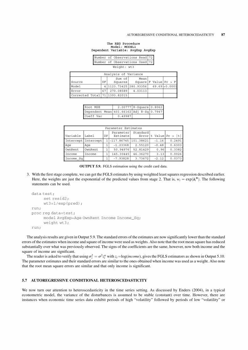
3. With the first stage complete, we can get the FGLS estimates by using weighted least squares regression described earlier.
Here, the weights are just the exponential of the predicted values from stage 2. That is, wi ¼ expðziaÞ. The following
statements can be used.
data test;
set resid2;
wt3=1/exp(pred);
run;
proc reg data=test;
model AvgExp=Age OwnRent Income Income_Sq;
weight wt3;
run;
The analysis results are given in Output 5.9. The standard errors of the estimates are now significantly lower than the standard
errors of the estimates when income and square of incomewere used as weights. Also note that the root mean square has reduced
substantially over what was previously observed. The signs of the coefficients are the same, however, now both income and the
square of income are significant.
The reader is asked to verify that using s2i ¼ s2zai with zi¼log(income), gives the FGLS estimators as shown in Output 5.10.
The parameter estimates and their standard errors are similar to the ones obtained when incomewas used as a weight. Also note
that the root mean square errors are similar and that only income is significant.
5.7 AUTOREGRESSIVE CONDITIONAL HETEROSCEDASTICITY
We now turn our attention to heteroscedasticity in the time series setting. As discussed by Enders (2004), in a typical
econometric model, the variance of the disturbances is assumed to be stable (constant) over time. However, there are
instances when economic time series data exhibit periods of high “volatility” followed by periods of low “volatility” or
The REG ProcedureModel: MODEL1
Dependent Variable: AvgExp AvgExp
The REG ProcedureModel: MODEL1
Dependent Variable: AvgExp AvgExp
Number of Observations Read 72
Number of Observations Used 72
Weight: wt3
Analysis of Variance
Source DFSum of
SquaresMean
Square F Value Pr > F
Model 4 1123.73425 280.93356 69.69 <0.0001
Error 67 270.08589 4.03113
Corrected Total 71 1393.82015
Root MSE 2.00777 R-Square 0.8062
Dependent Mean 401.66162 Adj R-Sq 0.7947
Coeff Var 0.49987
Parameter Estimates
Variable Label DFParameterEstimate
StandardError t Value Pr > |t|
Intercept Intercept 1 –117.86745 101.38621 –1.16 0.2491
Age Age 1 –1.23368 2.55120 –0.48 0.6303
OwnRent OwnRent 1 50.94976 52.81429 0.96 0.3382
Income Income 1 145.30445 46.36270 3.13 0.0026
Income_Sq 1 –7.93828 3.73672 –2.12 0.0373
OUTPUT 5.9. FGLS estimation using the credit card data.
AUTOREGRESSIVE CONDITIONAL HETEROSCEDASTICITY 87

“calmness.” Greene (2003, p. 238) analyzes the well-known Bollerslev and Ghysel�s data on the daily percentage nominal
return for the Deuschmark/Pound exchange rate. We analyzed the data using SAS—Figure 5.4 shows that there are periodic
spikes in the data on both the high and low sides. It is obvious that the variability appears to be unstable or shifting over
time. In particular, large shocks appear to follow each other and vice versa, small shocks appear to follow each other. The
variance of the disturbance at a given time period is therefore assumed to depend on the variance of the disturbance in the
previous time periods. Therefore, the homoscedastic variance assumption in this case is violated. The disturbance terms in
the linear models must therefore take into account the dependence of its variance on past disturbances. This is the basic
principle behind Engle�s (1982) autoregressive, conditionally heteroscedastic models (ARCH). He proposed a methodology
where the variance of the disturbances ð«tÞ are allowed to depend on its history. That is, the variance of the series itself is anautoregressive time series.
Bollerslev (1986) extended the ARCH process by allowing an autoregressive moving average process for the error variance.
Their resulting formulation is referred to as the generalized autoregressive conditional heteroscedastic model or GARCH. Both
the ARCH and the GARCH models forecast the variance of the disturbance at time t. The ARCH models uses the weighted
averages of the past values of the squared disturbances, while the GARCHmodel uses theweighted average of the past values of
both the squared disturbances and the variances.
5.7.1 The Arch Model
The simplest formofEngle�sARCHmodel is theARCH(1)model.Themain ideabehind themodel is that the conditional variance
of the disturbance at time t depends on the squared disturbance term at time t� 1. To see this, first, consider the basicmodel given
by yt ¼ stzt, where zt � i:i:d:Nð0; 1Þ. In an ARCH(1) model, s2t ¼ a0 þ a1y
2t�1 where a0 > 0 and a1 � 0. It can be shown
that
Eðytjyt�1Þ ¼ 0 and Varðytjyt�1Þ ¼ a0 þ a1y2t�1:
The REG ProcedureModel: MODEL1
Dependent Variable: AvgExp AvgExp
The REG ProcedureModel: MODEL1
Dependent Variable: AvgExp AvgExp
Number of Observations Read 72
Number of Observations Used 72
Weight: wt4
Analysis of Variance
Source DFSum of
SquaresMean
Square F Value Pr > F
Model 4 562700 140675 5.69 0.0005
Error 67 1655217 24705
Corrected Total 71 2217918
Root MSE 157.17741 R-Square 0.2537
Dependent Mean 216.57420 Adj R-Sq 0.2092
Coeff Var 72.57439
Parameter Estimates
Variable Label DFParameterEstimate
StandardError t Value Pr > |t|
Intercept Intercept 1 –193.27961 171.06009 –1.13 0.2626
Age Age 1 –2.95778 4.76203 –0.62 0.5366
OwnRent OwnRent 1 47.37065 72.12961 0.66 0.5136
Income Income 1 208.84940 77.19611 2.71 0.0086
Income_Sq 1 –12.76626 8.08456 –1.58 0.1190
OUTPUT 5.10. FGLS estimation using zi¼log(income) for the credit card data.
88 NONSPHERICAL DISTURBANCES AND HETEROSCEDASTICITY

Therefore, the conditional variance of the disturbance at time t depends on the past values of the squared disturbances. The
unconditional variance on the other hand is constant. To see this note thatVarðytÞ ¼ Eðy2t Þ ¼ a0 þ a1Eðy2t�1Þ. Simplifying this
gives VarðytÞ ¼ a0=ð1� a1Þ, a0 > 0, 0 � a1 < 1.
The ARCH(1) process can easily be extended to linear models with explanatory variables. First, consider the linear model
yt ¼ xTt bþ «t with «t ¼ stzt, where zt � i:i:d:Nð0; 1Þ ands2t ¼ a0 þ a1«
2t�1. It can be easily shown that the conditional variance
VarðytjxtÞ ¼ a0 þ a1«2t�1 while the unconditional variance VarðytÞ ¼ Varð«tÞ ¼ a0=ð1�a1Þwith 0 � a1 < 1 (Greene, 2003,
pp. 238–239)
5.7.2 ARCH(q) and the Generalized ARCH Models
Extending the simple ARCH(1) model to the more general case we get the ARCH(q) process given by yt ¼ stzt, where
zt � i:i:d:Nð0; 1Þ and
s2t ¼ a0 þ
X
q
i¼1
aiy2t�i:
Note that the unconditional variance is now given by
Var «tð Þ ¼ a0= 1�X
q
i¼1
ai
!
with 0 �X
q
i¼1
ai < 1:
The ARCH(q) process can easily be extended to the linear regression setting in a similar fashion.
5.7.3 The GARCH Model
Bollerslev (1986) extended theARCHmodelswhere the variance of the disturbance at time t depends on its own lag aswell as the
lag of the squared disturbances. In the GARCH(1,1) model,
s2t ¼ a0 þ a1«
2t�1 þ b1s
2t�1:
y
-3
-2
-1
0
1
2
3
4
Obs
0 200 400 600 800 1000 1200 1400 1600 1800 2000
FIGURE 5.4. Time series plot for the nominal returns.
AUTOREGRESSIVE CONDITIONAL HETEROSCEDASTICITY 89

The basic principle is to make the forecast of the variance at time t more accurate. In a GARCH(p,q) model
s2t ¼ a0 þ
X
p
i¼1
dis2t�i þ
X
q
j¼1
aj«2t�j:
It can be shown that the unconditional variance of the disturbance at time t is
s2« ¼
a0
1�P
q
i¼1
ai�P
p
j¼1
bj
where a0 � 0, ai � 0, bi � 0, and 0 � 1�P
q
i¼1
ai�P
p
j¼1
bj < 1.
The GARCH(p,q) models can easily be extended to the linear regression setting as well.
5.7.4 Testing for ARCH Effects
The Lagrange Multiplier test (LM) can be used to test for ARCH(q) effects. The hypothesis tested is
H0 : a1 ¼ a2 ¼ . . . ¼ aq ¼ 0
H1 : at least one ai 6¼ 0;i ¼ 1; . . . q:
The steps are as follows:
1. Estimate yt ¼ xTt bþ «t using OLS and calculate «2t�i for i ¼ 1; . . . ; q.
2. Conduct a regression of «2t on a constant and «2t�1; . . . ; «2t�q and calculate the coefficient of determination, R2.
3. Calculate the test statistic TR2, where T is the number of observations. Under the null hypothesis, TR2 � x2q. We reject the
null hypothesis of noARCHeffects if the calculated value of the test statistic exceeds the tabled value from the chi-squared
distribution.
The LM test can also be used for testing GARCH effects. In a test for a GARCH(p,q) model, however, the hypothesis tested is
thenull ofaARCH(q) process versus aARCH(p+q) process (Baltagi, 2008, p. 370).Here, theLMtest is basedon the regressionof
«2t on p + q lagged values «2t�1; . . . ; «2t�p�q. The test statistic is the same as before.
Maximum likelihood estimation can be used to estimate the parameters of both theARCHandGARCHmodels.Details can be
found in Greene (2003) page 239 (ARCH) and pages 242–243 (GARCH).
Wewill now illustrate the estimation of these models in SAS by using the Bollerslev and Ghysels nominal exchange rate data.
For illustration purposes, we will use a GARCH(1,1) model.
The ProcAutoregmodule in SAS can be used to fit this model. Recall that this procedure should be used to perform regression
analysis when the underlying assumption of heteroscedasticity and autocorrelation are violated. It can also be used to perform
ARCH andGARCH calculations. First, wewill use the procedure to test for heteroscedasticity in the data by using the “archtest”
option. The following commands can be used. Note that a temporary SAS data set named “garch”was created prior to invoking
this procedure. The analysis results are given in Output 5.11.
proc autoreg data=garch;
model y=/archtest;
run;
The first table of the output gives the OLS estimates. The values for SSE andMSE are for the error and mean sums of squares.
The MSE is really the unconditional variance of the series. The Durbin–Watson statistic is used to test for serial correlation and
90 NONSPHERICAL DISTURBANCES AND HETEROSCEDASTICITY

will be discussed in detail in Chapter 6. DFE is simply the degrees of freedom and is the total number of observations �1. The
values ofAICandBICare information criteriavalues that are used to assessmodel fit. Smaller values of the statistics are desirable.
The Durbin–Watson statistics will be discussed in Chapter 6.
The output also contains the Q and LM tests. Both statistics test for heteroscedasticity in the time series. The
Q statistic proposed by McLeod and Li (1983) (see the Proc Autoreg reference guide from SAS Institute) checks for
changing variability over time. The test is highly significant across the 12 lag windows. The LM statistic was discussed earlier.
It is also highly significant across all 12 lag windows indicating that a higher order ARCH process needs to be used to model
the data.
As discussed earlier, the GARCH process introduces the lagged values of the variances also and thus introduces a “longer
memory” (Proc Autoreg reference guide, SAS Institute, Inc.). Therefore, we start our initial model at the GARCH(1,1)
process. The following statements can be used. Note that the option “garch” can be changed to allow for anARCHprocess. For
example, using the option “garch=(q=1)” will request an ARCH(1) process for the dataset. The analysis results are given in
Output 5.12.
proc autoreg data=garch;
model y=/Garch=(p=1,q=1);
run;
The output indicates that there is strong evidence of GARCH effects (p value < 0.0001). The unconditional
variance for the GARCH model is 0.2587 compared to 0.2211 for the OLS model. The normality test is highly significant
The AUTOREG Procedure
Dependent Variable y
y
Ordinary Least Squares Estimates
SSE 436.289188 DFE 1973
MSE 0.22113 Root MSE 0.47024
SBC 2629.78062 AIC 2624.1928
Regress R-Square 0.0000 Total R-Square 0.0000
Durbin-Watson 1.9805
Q and LM Tests for ARCH Disturbances
Order Q Pr > Q LM Pr > LM
1 96.4249 <0.0001
<0.0001
<0.0001
<0.0001
<0.0001
<0.0001
<0.0001
<0.0001
<0.0001
<0.0001
<0.0001
<0.0001
<0.0001
<0.0001
<0.0001
<0.0001
<0.0001
<0.0001
<0.0001
<0.0001
<0.0001
<0.0001
<0.0001
<0.0001
96.3422
2 157.1627 129.5878
3 196.7515 142.6618
4 227.4684 150.3655
5 297.7401 183.3808
6 314.1284 183.3929
7 328.6768 183.8867
8 347.5464 186.8223
9 364.7738 188.8952
10 392.9791 194.1606
11 397.5269 194.9219
12 404.9266 195.1401
Variable DF EstimateStandard
Error t ValueApprox
Pr > |t|
Intercept 1 –0.0164 0.0106 –1.55 0.1208
OUTPUT 5.11. Testing for the heteroscedasticity in the nominal exchange data.
AUTOREGRESSIVE CONDITIONAL HETEROSCEDASTICITY 91

(p value < 0.0001), which indicates that the residuals from the GARCH model are not normally distributed—a clear
contradiction to the normality assumption. ARCH0 gives the estimate of a0, ARCH1 gives the estimate of a1, and GARCH1
gives the estimate of b1.
The AUTOREG Procedure
Dependent Variable y
y
Ordinary Least Squares Estimates
SSE 436.289188 DFE 1973
MSE 0.22113 Root MSE 0.47024
SBC 2629.78062 AIC 2624.1928
Regress R-Square 0.0000 Total R-Square 0.0000
Durbin-Watson 1.9805
Variable DF EstimateStandard
Error t ValueApprox
Pr > |t|
Intercept 1 –0.0164 0.0106 –1.55 0.1208
Algorithm converged.
GARCH Estimates
SSE 436.495992 Observations 1974
MSE 0.22112 Uncond Var 0.25876804
Log Likelihood –1106.6908 Total R-Square .
SBC 2243.73289 AIC 2221.38163
Normality Test 1081.7663 Pr > ChiSq <0.0001
Variable DF EstimateStandard
Error t ValueApprox
Pr > |t|
Intercept 1 –0.006191 0.008426 –0.73 0.4625
ARCH0 1 0.0108 0.001327 8.15 <0.0001
ARCH1 1 0.1524 0.0139 10.97 <0.0001
GARCH1 1 0.8058 0.0166 48.61 <0.0001
OUTPUT 5.12. GARCH (1, 1) model for the nominal exchange rate data.
92 NONSPHERICAL DISTURBANCES AND HETEROSCEDASTICITY

6AUTOCORRELATION
6.1 INTRODUCTION
In Chapters 4 and 5 we discussed estimation methods for b under departures from the exogeneity and homoscedasticity
assumptions. This chapter extends the discussion to the casewhen the assumption of independent disturbances is violated. That is,
we will relax the assumption that the disturbance related to an observation is independent of the disturbance related to another
observation. We call this situation serial correlation or autocorrelation. Simply put, in autocorrelation Cov(«t, «s) „ 0 for t „ s
where t and s are two time periods. Autocorrelationmost often occurs in time series data where the observation at a given point in
time is dependent on the observations from the previous time periods
The texts by Greene (2003, Chapter 12), Meyers (1990, Chapter 7), and Verbeek (2004, Chapter 4) offer a good discussion on
autocorrelationmodels. Brocklebank andDickey (2003) offer a thorough treatment of howSAS can be used to fit autocorrelation
models.
Autocorrelation in regression models often occurs when models are misspecified or when variables are mistakenly omitted
from themodel. In the omitted variable case, unobserved or omitted variables that are correlated over time are nowabsorbed in the
error term, causing autocorrelation. As an example, consider the gasoline consumption data in Greene (2003). Gasoline
consumption along with measurements on other variables was observed from 1960 to 1995. Note that this data was analyzed in
Chapter 2. The full equation for this model is (Greene, 2003, p. 136)
lnðGt=PoptÞ ¼ b1 þb2lnðPgtÞþb3lnðIt=PoptÞþb4lnðPnctÞþb5lnðPuctÞ
þb6lnðPpTtÞþb7lnðPNtÞþb8lnðPDtÞþb9lnðPStÞþb10tþ «t:
Assume that we fit the model
lnðGt=PoptÞ ¼ b1 þb2lnðPgtÞþb3lnðIt=PoptÞþb4lnðPnctÞþb5lnðPuctÞþ «t:
The residuals from the fittedmodel and the fullmodel are shown inFigures6.1 and6.2.Note that the residuals frombothmodels
show that autocorrelation should be investigated. However, the fitted model shows a higher degree of autocorrelation.
93
Applied Econometrics Using the SAS� System, by Vivek B. AjmaniCopyright � 2009 John Wiley & Sons, Inc.

Although, time series plots of the residuals (as the ones above) can be used to detect autocorrelation issues quickly, we will
discuss more formal procedures to detect the presence of autocorrelation in the data.
6.2 PROBLEMS ASSOCIATED WITH OLS ESTIMATION UNDER AUTOCORRELATION
We start our discussion of estimation under autocorrelation by considering the simple autoregressive first-order autocorrelation
model (AR1)with exogenous explanatory variables. That is, amodel of the form yi ¼ xTi bþ «ii ¼ 1; 2; . . . , with «i ¼ r«i�1 þ ui
LS Residuals versus Year
0.04
0.03
0.02
0.01
0.00Res
idu
als
–0.01
–0.02
–0.03
1960 1970 1980
Year
1990 2000
FIGURE 6.1. Time series plot of the residuals from the full model in the gasoline consumption data.
LS Residuals versus Year
0.05
0.04
0.03
0.02
0.01
0.00
–0.01
Res
idu
als
–0.02
–0.03
–0.04
–0.05
–0.06
1960 1970 1980
Year
1990 2000
FIGURE 6.2. Time series plot of the residuals from the reduced model in the gasoline consumption data.
94 AUTOCORRELATION

where jrj<1 is required to ensure Varð«tÞ < 1 . Assume that EðuiÞ ¼ 0 , VarðuiÞ ¼ s2 , and Covðut; usÞ ¼ 0 for t 6¼ s . That is,
the error term ui hasmean zero, has constant variance, and exhibits no serial correlation. It can be easily shown thatEð«iÞ ¼ 0 and
that thevarianceVarð«iÞ ¼ s2u=ð1� r2Þwhere jrj<1.Also note that the covariance between «i and «i�1 denoted byCovð«i; «i�1Þ
is given by
Covð«i; «i�1Þ ¼ rs2u
1� r2
and that the covariance between two disturbances, which are two periods apart, Covð«i; «i�2Þ is given by
Covð«i; «i�2Þ ¼ r2s2u
1� r2:
Extending this to two disturbances, which are j time periods apart, we get Covð«i; «i�jÞ given by
Covð«i; «i�jÞ ¼s2u
1� r2rj:
Autocorrelation therefore implies that the errors are heteroscedastic (Greene, 2003, p. 258; Meyers, 1990, p. 289). As shown in
Chapter 5, OLS estimators, although unbiased will be inefficient and will have incorrect standard errors.
yi ¼ xTi bþ «i; i ¼ 1; 2; . . . ;
«i ¼ r«i�1 þ ui;
6.3 ESTIMATION UNDER THE ASSUMPTION OF SERIAL CORRELATION
Estimation techniques under the assumption of serial correlation parallel the estimation methods for heteroscedasticity that was
discussed inChapter 5. That is, we need to first estimate thevariance–covariancematrix. Using thevariance and covariance of the
disturbances given in the previous section, we can easily construct the covariance matrix s2V as (Greene, 2003, p. 259)
s2V ¼s2u
1�r2
1 r r2 r3 . . . rT�1
r 1 r r2 . . . rT�2
r2 r 1 r . . . rT�3
.
.
....
.
.
...
....
.
.
.
.
.
....
.
.
....
..
.r
rT�1 rT�2 rT�3. . . r 1
2
6
6
6
6
6
6
6
6
6
6
4
3
7
7
7
7
7
7
7
7
7
7
5
:
If r is known, then using the discussion from Chapter 5, one can get a GLS estimator of b as
bGLS ¼ ðXTV�1XÞ�1
XTV�1y:
It can be shown that the GLS estimator is an unbiased, consistent estimator for b with variance-covariance matrix given by
Est:Var½bGLS� ¼ s2«½X
TV�1X��1;
ESTIMATION UNDER THE ASSUMPTION OF SERIAL CORRELATION 95

where
s2« ¼
ðy�XbGLSÞTV�1ðy�XbGLSÞ
TðGreene; 2003; p: 271Þ:
These computations can be carried out easily by simply transforming y andX and runningOLSon the transformed values. The
transformations for the first-order autocorrelation process are
y�1 ¼ffiffiffiffiffiffiffiffiffiffiffiffiffi
1� r2p
y1 and x�1 ¼ffiffiffiffiffiffiffiffiffiffiffiffiffi
1� r2p
x1 for t ¼ 1;
y�t ¼ yt � ryt�1 and x�t ¼ xt � rxt�1 for t ¼ 2; . . . ; T ðGreene; 2003; p: 272Þ:
These transformations are called the Prais–Winsten transformations. The traditional approach (Cochrane and Orcutt, 1949)
used the same transformation but dropped the first observation for computational ease. As discussed in Verbeek (2004, p. 100),
deleting the observation leads to an approximateGLS estimator that is not as efficient as theGLS estimator obtained by including
all the observations.
The GLS estimator can then be calculated as follows:
bGLS ¼ ðXT� X�Þ
�1XT� y�:
Greene (2003) extends the process to the second-order autocorrelation process. As can be seen from the transformation formulas
the author provides, the process becomes very complex as the order of the autoregressive process increases.
The estimation techniques discussed so far are based on the assumption that r is known. However, in reality, r is unknown and
has to be estimated. Estimation of the least squares parameters is straightforward under the assumption that r is unknown. In the
case of the first-order autocorrelation model, the steps are as follows:
1. Estimate the model yi ¼ xTi bþ «i; i ¼ 1; 2; . . . using OLS and save the residuals.
2. Using the residuals, fit the model «i ¼ r«i�1 þ ui and get an estimate of r.
3. Use the residuals from Step 2 to estimate s2u. We can use the estimated values of r and s2
u to constructV^
. This can then
be used to calculate a FGLS estimator of b. Another alternative is to simply use the estimated value of r to transform
both y and X using the Prais–Winsten transformation and then conduct OLS with the transformed values (Greene,
2003, p. 273).
TheProcAutoregprocedure inSASwill allowus to estimate the least squares parameters byFGLS,MLE, or the iterated FGLS
method.Wewill discuss ways of conducting the analysis in SAS a bit later. For now, let us discussmethods of finding outwhether
the regression model suffers from autocorrelation.
6.4 DETECTING AUTOCORRELATION
TheDurbin–Watson test is perhaps themost commonly used test for detecting autocorrelation. It is based on the statistic (Meyers,
1990, p. 289)
DW ¼
P
T
i¼2
ð«i�«i�1Þ2
P
T
i¼1
«2i
and tests the hypothesis
H0 : r ¼ 0;
H1 : r 6= 0:
ProcAutoregcanbeused to conduct theDurbin–Watson test.On theother hand, even thoughProcRegdoes give thevalue of the
test statistic and the estimated first-order correlation, it does not output the p value associated with the test.
96 AUTOCORRELATION

The Lagrange multiplier test suggested by Breusch and Godfrey (1978) is an alternative to the Durbin–Watson test. The test
statistic is LM ¼ TR2, where R2 is the R-squared value obtained by regressing the OLS residuals against p-lagged residuals
«t�1; . . . ; «t�p along with the original variables in X where the residuals can be obtained by OLS. The test statistic has a chi-
squared distribution with p degrees of freedom.
Twoother alternatives to theDurbin–Watson test are theBox and Pierce�s test (B&P) andLjung�smodification of the B&P test
(Greene 2003, p. 269). The B&Q test is based on the test statistic
Q ¼ TX
p
j¼1
r2j ;
where
rj ¼
P
T
t¼jþ 1
etet�j
P
T
t¼1
e2t
:
That is, rj measures the autocorrelation between et and et�j. This test statistic has a limiting chi-squared distribution with p
degrees of freedom. Here, p refers to the number of lags used.
As stated in Greene (2003, p. 269) the Ljung�s refinement of the B&P test is given by
Q0 ¼ TðT þ 2ÞX
p
j¼1
r2j
T�j;
where rj is defined as before. This test statistic has a chi-squared distribution with p degrees of freedom also.
We will now illustrate the computations involved by analyzing the gas consumption data in Greene (2003). We restrict our
attention to the reduced model
lnðGt=PoptÞ ¼ b1 þb2lnðPgtÞþb3lnðIt=PoptÞþb4lnðPnctÞþb5lnðPuctÞþ «t
to force some autocorrelation behavior. The following SAS statements can be used to fit the OLS model to the data and
also compute the Durbin–Watson and Breusch–Godfrey statistic along with their p values. The “dwprob” and “godfrey” options
are used to generate the statistics. The analysis results are given in Output 6.1.
proc autoreg data=gasoline;
model Ln_G_Pop=Ln_Pg Ln_Income Ln_Pnc Ln_Puc/dwprob
godfrey;
run;
Both tests indicate a presence of autocorrelation in the data. The p value for theDurbin–Watson test indicates the presence of a
positive autocorrelation. The LM test indicates that the significance extends to the higher order AR(4). Adding the option
“dw¼ 5” to the model statement yields the Durbin–Watson statistics for the first five autocorrelations. The analysis results are
given in Output 6.2. Note that there is strong evidence of a positive first-order correlation.
We can use the correlations calculated by Proc Autoreg to conduct the B&P test and the Ljung test. First, we calculate the first
five autocorrelations by using the following statements (see Output 6.3):
proc autoreg data=gasoline;
model Ln_G_Pop=Ln_Pg Ln_Income Ln_Pnc Ln_Puc/nlag=5;
run;
DETECTING AUTOCORRELATION 97

The AUTOREG Procedure
Dependent Variable Ln_G_Pop
Ordinary Least Squares Estimates
SSE 0.02487344 DFE 31
MSE 0.0008024 Root MSE 0.02833
SBC –141.90789 AIC –149.82548
Regress R-Square 0.9691 Total R-Square 0.9691
Durbin–Watson Statistics
Order DW Pr < DW Pr > DW
1 0.8909 <0.0001 1.0000
2 2.0276 0.4049 0.5951
3 2.3773 0.8792 0.1208
4 2.1961 0.8211 0.1789
5 1.9231 0.6318 0.3682
Note: Pr < DW is the p value for testing positive autocorrelation, and Pr > DW is the p value for testing negative autocorrelation.
Variable DF EstimateStandard
Error t ValueApproxPr > |t|
Intercept 1 –7.7892 0.3593 –21.68 <0.0001
Ln_pg 1 –0.0979 0.0283 –3.46 0.0016
Ln_Income 1 2.1175 0.0988 21.44 <0.0001
Ln_Pnc 1 0.1224 0.1121 1.09 0.2830
Ln_Puc 1 –0.1022 0.0693 –1.48 0.1502
OUTPUT 6.2. Durbin–Watson statistics for the first five autocorrelations in the gasoline data.
The AUTOREG Procedure
Dependent Variable Ln_G_Pop
Ordinary Least Squares Estimates
SSE 0.02487344 DFE 31
MSE 0.0008024 Root MSE 0.02833
SBC –141.90789 AIC –149.82548
Regress R-Square 0.9691 Total R-Square 0.9691
Durbin–Watson 0.8909 Pr < DW <0.0001
Pr > DW 1.0000
Note: Pr < DW is the p value for testing positive autocorrelation, and Pr > DW is the p value for testing negative autocorrelation.
Godfrey's Serial CorrelationTest
Alternative LM Pr > LM
AR(1) 11.2170 0.0008
AR(2) 17.1932 0.0002
AR(3) 17.2414 0.0006
AR(4) 17.6825 0.0014
Variable DF EstimateStandard
Error t ValueApproxPr > |t|
Intercept 1 –7.7892 0.3593 –21.68 <0.0001
Ln_pg 1 –0.0979 0.0283 –3.46 0.0016
Ln_Income 1 2.1175 0.0988 21.44 <0.0001
Ln_Pnc 1 0.1224 0.1121 1.09 0.2830
Ln_Puc 1 –0.1022 0.0693 –1.48 0.1502
OUTPUT 6.1. Using Proc Autoreg to detect autocorrelation in the gasoline data.
98 AUTOCORRELATION

The AUTOREG Procedure
Dependent Variable Ln_G_Pop
Ordinary Least Squares Estimates
SSE 0.02487344 DFE 31
MSE 0.0008024 Root MSE 0.02833
SBC –141.90789 AIC –149.82548
Regress R-Square 0.9691 Total R-Square 0.9691
Durbin–Watson 0.8909
Variable DF EstimateStandard
Error t ValueApproxPr > |t|
Intercept 1 –7.7892 0.3593 –21.68 <0.0001
Ln_pg 1 –0.0979 0.0283 –3.46 0.0016
Ln_Income 1 2.1175 0.0988 21.44 <0.0001
Ln_Pnc 1 0.1224 0.1121 1.09 0.2830
Ln_Puc 1 –0.1022 0.0693 –1.48 0.1502
Estimates of Autocorrelations
Lag Covariance Correlation −1 9 8 7 6 5 4 3 2 1 0 1 2 3 4 5 6 7 8 9 1
0 0.000691 1.000000 | |********************|
1 0.000382 0.552840 | |*********** |
2 −0.00001 –0.021286 | | |
3 −0.00015 –0.211897 | ****| |
4 −0.00010 –0.147596 | ***| |
5 −0.00002 –0.025090 | *| |
Preliminary MSE 0.000365
Estimates of AutoregressiveParameters
Lag CoefficientStandard
Error t Value
1 –0.883472 0.195936 –4.51
2 0.623294 0.260538 2.39
3 –0.217351 0.284615 –0.76
4 0.117484 0.260538 0.45
5 –0.042809 0.195936 –0.22
Yule–Walker Estimates
SSE 0.01258864 DFE 26
MSE 0.0004842 Root MSE 0.02200
SBC –147.56116 AIC –163.39635
Regress R-Square 0.9568 Total R-Square 0.9844
Durbin–Watson 1.8728
Variable DF EstimateStandard
Error t ValueApproxPr > |t|
Intercept 1 –7.5542 0.4583 –16.48 <0.0001
Ln_pg 1 –0.0706 0.0337 –2.09 0.0461
Ln_Income 1 2.0520 0.1259 16.30 <0.0001
Ln_Pnc 1 0.1344 0.1336 1.01 0.3239
Ln_Puc 1 –0.1257 0.0833 –1.51 0.1434
OUTPUT 6.3. Proc Autoreg output showing the first five autocorrelations from the gasoline data.
DETECTING AUTOCORRELATION 99

The AUTOREG Procedure
Dependent Variable Ln_G_Pop
Ordinary Least Squares Estimates
SSE 0.02487344 DFE 31
MSE 0.0008024 Root MSE 0.02833
SBC –141.90789 AIC –149.82548
Regress R-Square 0.9691 Total R-Square 0.9691
Durbin–Watson 0.8909 Pr < DW <0.0001
Pr > DW 1.0000
Note: Pr < DW is the p value for testing positive autocorrelation, and Pr > DW is the p value for testing negative autocorrelation.
Variable DF EstimateStandard
Error t ValueApproxPr > |t|
Intercept 1 −7.7892 0.3593 −21.68 <0.0001
Ln_pg 1 −0.0979 0.0283 −3.46 0.0016
Ln_Income 1 2.1175 0.0988 21.44 <0.0001
Ln_Pnc 1 0.1224 0.1121 1.09 0.2830
Ln_Puc 1 −0.1022 0.0693 −1.48 0.1502
Estimates of Autocorrelations
Lag Covariance Correlation -1 9 8 7 6 5 4 3 2 1 0 1 2 3 4 5 6 7 8 9 1
0 0.000691 1.000000 | |********************|
1 0.000382 0.552840 | |*********** |
Preliminary MSE 0.000480
Estimates of AutoregressiveParameters
Lag CoefficientStandard
Error t Value
1 –0.552840 0.152137 –3.63
Yule–Walker Estimates
SSE 0.01604701 DFE 30
MSE 0.0005349 Root MSE 0.02313
SBC –153.73763 AIC –163.23874
Regress R-Square 0.9271 Total R-Square 0.9801
Durbin–Watson 1.3707 Pr < DW 0.0077
Pr > DW 0.9923
Note: Pr < DW is the p value for testing positive autocorrelation, and Pr > DW is the p value for testing negative autocorrelation.
Variable DF EstimateStandard
Error t ValueApproxPr > |t|
Intercept 1 −7.1940 0.5152 −13.96 <0.0001
Ln_pg 1 −0.1239 0.0366 −3.39 0.0020
Ln_Income 1 1.9534 0.1418 13.77 <0.0001
Ln_Pnc 1 0.1221 0.1317 0.93 0.3611
Ln_Puc 1 −0.0548 0.0784 −0.70 0.4900
OUTPUT 6.4. AR(1) model for the gasoline consumption data.
100 AUTOCORRELATION

The B&P test statistic value is
Q ¼ 36� b0:55282 þ 0:02132 þ 0:2122 þ 0:14762 þ 0:02512c ¼ 13:44;
while the Ljung test statistic value is
Q0 ¼ 36� 38�0:55282
35þ
0:02132
34þ
0:2122
33þ
0:14762
32þ
0:02512
31
� �
¼ 14:78:
Both test statistic values exceed the chi-squared critical value ofx20:05;5 ¼ 11:07 leading to the rejectionof the null hypothesis of
no autocorrelation. Therefore, the OLS estimates are not efficient and we need to get estimates that are adjusted for the
autocorrelations.
6.5 USING SAS TO FIT THE AR MODELS
Having detected the presence of autocorrelation, we must now estimate the parameters by using either GLS or FGLS. As
mentioned in the earlier sections, in reality r is assumed to be unknown and therefore has to be estimated leading to the FGLS
estimator.Wewill use Proc Autoreg to fit the ARmodels. In this instance, we use it to conduct OLS regression where we suspect
that the disturbances are correlated. Proc Reg can also be used to conduct the analysis. However, the data will have to be first
transformed by using the Prais–Winsten (or the Cochrane and Orcutt) methods. The following statements can be used to fit the
AR (1) model to the gasoline consumption data set. The “nlag¼1” option requests the AR(1) model while the options “dw” and
“dwprob” are used for the Durbin–Watson test statistic and p values. The analysis results are given in Output 6.4.
The AUTOREG Procedure
Dependent Variable Ln_G_Pop
Ordinary Least Squares Estimates
SSE 0.02487344 DFE 31
MSE 0.0008024 Root MSE 0.02833
SBC –141.90789 AIC –149.82548
Regress R-Square 0.9691 Total R-Square 0.9691
Durbin–Watson Statistics
Order DW Pr < DW Pr > DW
1 0.8909 <0.0001 1.0000
2 2.0276 0.4049 0.5951
Note: Pr<DW is the p value for testing positive autocorrelation, and Pr>DW is the p value for testing negative autocorrelation.
Variable DF EstimateStandard
Error t ValueApproxPr > |t|
Intercept 1 –7.7892 0.3593 –21.68 <0.0001
Ln_pg 1 –0.0979 0.0283 –3.46 0.0016
Ln_Income 1 2.1175 0.0988 21.44 <0.0001
Ln_Pnc 1 0.1224 0.1121 1.09 0.2830
Ln_Puc 1 –0.1022 0.0693 –1.48 0.1502
Estimates of Autocorrelations
Lag Covariance Correlation −1 9 8 7 6 5 4 3 2 1 0 1 2 3 4 5 6 7 8 9 1
0 0.000691 1.000000 | |********************|
1 0.000382 0.552840 | |*********** |
2 –0.00001 –0.021286 | | |
Preliminary MSE 0.000373
OUTPUT 6.5. AR(2) model for the gasoline consumption data.
USING SAS TO FIT THE AR MODELS 101
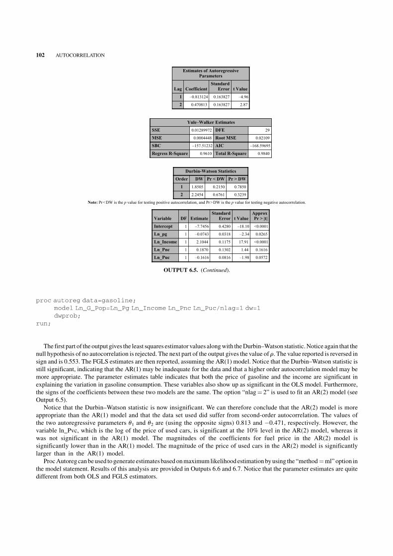
proc autoreg data=gasoline;
model Ln_G_Pop=Ln_Pg Ln_Income Ln_Pnc Ln_Puc/nlag=1 dw=1
dwprob;
run;
The first part of the output gives the least squares estimator values alongwith theDurbin–Watson statistic.Notice again that the
null hypothesis of no autocorrelation is rejected. The next part of the output gives the value of r. The value reported is reversed in
sign and is 0.553. The FGLS estimates are then reported, assuming the AR(1) model. Notice that the Durbin–Watson statistic is
still significant, indicating that the AR(1) may be inadequate for the data and that a higher order autocorrelation model may be
more appropriate. The parameter estimates table indicates that both the price of gasoline and the income are significant in
explaining the variation in gasoline consumption. These variables also show up as significant in the OLS model. Furthermore,
the signs of the coefficients between these two models are the same. The option “nlag¼ 2” is used to fit an AR(2) model (see
Output 6.5).
Notice that the Durbin–Watson statistic is now insignificant. We can therefore conclude that the AR(2) model is more
appropriate than the AR(1) model and that the data set used did suffer from second-order autocorrelation. The values of
the two autoregressive parameters u1 and u2 are (using the opposite signs) 0.813 and �0.471, respectively. However, the
variable ln_Pvc, which is the log of the price of used cars, is significant at the 10% level in the AR(2) model, whereas it
was not significant in the AR(1) model. The magnitudes of the coefficients for fuel price in the AR(2) model is
significantly lower than in the AR(1) model. The magnitude of the price of used cars in the AR(2) model is significantly
larger than in the AR(1) model.
ProcAutoregcanbeused to generate estimates based onmaximum likelihoodestimationbyusing the “method¼ml”option in
the model statement. Results of this analysis are provided in Outputs 6.6 and 6.7. Notice that the parameter estimates are quite
different from both OLS and FGLS estimators.
Estimates of AutoregressiveParameters
Lag CoefficientStandard
Error t Value
1 –0.813124 0.163827 –4.96
2 0.470813 0.163827 2.87
Yule–Walker Estimates
SSE 0.01289972 DFE 29
MSE 0.0004448 Root MSE 0.02109
SBC –157.51232 AIC –168.59695
Regress R-Square 0.9610 Total R-Square 0.9840
Durbin-Watson Statistics
Order DW Pr < DW Pr > DW
1 1.8505 0.2150 0.7850
2 2.2454 0.6761 0.3239
Note: Pr<DW is the p value for testing positive autocorrelation, and Pr>DW is the p value for testing negative autocorrelation.
Variable DF EstimateStandard
Error t ValueApproxPr > |t|
Intercept 1 –7.7456 0.4280 –18.10 <0.0001
Ln_pg 1 –0.0743 0.0318 –2.34 0.0265
Ln_Income 1 2.1044 0.1175 17.91 <0.0001
Ln_Pnc 1 0.1870 0.1302 1.44 0.1616
Ln_Puc 1 –0.1616 0.0816 –1.98 0.0572
OUTPUT 6.5. (Continued).
102 AUTOCORRELATION

The model statement option “method¼ ityw” will result in the iterated FGLS analysis. The results of the analysis are
provided in Outputs 6.8 and 6.9. Notice that the results are very similar to the results produced using maximum likelihood
estimation, thus confirming that in general the iterated estimation technique converges to the maximum likelihood estimates
(Greene, 2003).
It may be of interest to compare the predicted values from Proc Reg (OLS estimation) and Proc Autoreg.Wewill compare the
OLSpredicted valueswith the predicted values from theAR(2)model. The following statements can be used. The analysis results
are given in Figure 6.3.
proc reg data=gasoline noprint;
model Ln_G_Pop=Ln_Pg Ln_Income Ln_Pnc Ln_Puc;
output out=a r=r_g;
run;
proc autoreg data=gasoline noprint;
The AUTOREG Procedure
Dependent Variable Ln_G_Pop
Ordinary Least Squares Estimates
SSE 0.02487344 DFE 31
MSE 0.0008024 Root MSE 0.02833
SBC –141.90789 AIC –149.82548
Regress R-Square 0.9691 Total R-Square 0.9691
Durbin–Watson 0.8909 Pr < DW <0.0001
Pr > DW 1.0000
Note: Pr<DW is the p value for testing positive autocorrelation, and Pr>DW is the p value for testing negative autocorrelation.
Variable DF EstimateStandard
Error t ValueApproxPr > |t|
Intercept 1 –7.7892 0.3593 –21.68 <0.0001
Ln_pg 1 –0.0979 0.0283 –3.46 0.0016
Ln_Income 1 2.1175 0.0988 21.44 <0.0001
Ln_Pnc 1 0.1224 0.1121 1.09 0.2830
Ln_Puc 1 –0.1022 0.0693 –1.48 0.1502
Estimates of Autocorrelations
Lag Covariance Correlation −1 9 8 7 6 5 4 3 2 1 0 1 2 3 4 5 6 7 8 9 1
0 0.000691 1.000000 | |********************|
1 0.000382 0.552840 | |*********** |
Preliminary MSE 0.000480
Estimates of AutoregressiveParameters
Lag CoefficientStandard
Error t Value
1 –0.552840 0.152137 –3.63
Algorithm converged.
OUTPUT 6.6. MLE estimates of the AR(1) model for the gasoline consumption data.
USING SAS TO FIT THE AR MODELS 103

model Ln_G_Pop=Ln_Pg Ln_Income Ln_Pnc Ln_Puc/nlag=2;
output out=b r=ra_g;
run;
data c;
merge a b;
run;
proc gplot data=c;
plot r_g*year=1 ra_g*year=2/overlay href=0 haxis=1960 to
1995 by 5;
run;
It does appear that magnitudes of the residuals from OLS (solid line) have been reduced by using the AR(2)
model (dotted line) confirming that the AR(2) model is more appropriate for the gasoline consumption data set than the
OLS model.
In the discussion so far, we used an AR(2) model because the data set suffered from second-order autocorrelation. As it
turns out, there is not much gain (if any) in using a higher autocorrelation model. The following statements in SAS can be used
to compare the residuals from variousmodels. The “nlag¼” option with values 1 through 5 is used to fit models ranging from the
AR(1) to the AR(5) models. The residuals from each model are stored and compared against each other by using the “overlay”
option of Proc Gplot (Freund and Littell, 2000, p. 93). The analysis results are given in Figure 6.4.
proc autoreg data=gasoline noprint;
model Ln_G_Pop=Ln_Pg Ln_Income Ln_Pnc Ln_Puc/nlag=1;
output out=a r=r1;
Maximum Likelihood Estimates
SSE 0.01262941 DFE 30
MSE 0.0004210 Root MSE 0.02052
SBC –160.53233 AIC –170.03344
Regress R-Square 0.7830 Total R-Square 0.9843
Durbin–Watson 1.4455 Pr < DW 0.0193
Pr > DW 0.9807
Note: Pr<DW is the p value for testing positive autocorrelation, and Pr>DW is the p value for testing negative autocorrelation.
Variable DF EstimateStandard
Error t ValueApproxPr > |t|
Intercept 1 –5.1710 0.7617 –6.79 <0.0001
Ln_pg 1 –0.1939 0.0409 –4.74 <0.0001
Ln_Income 1 1.3896 0.2041 6.81 <0.0001
Ln_Pnc 1 0.2509 0.1480 1.70 0.1003
Ln_Puc 1 –0.004280 0.0698 –0.06 0.9515
AR1 1 –0.9425 0.0915 –10.30 <0.0001
Autoregressive parameters assumed given
Variable DF EstimateStandard
Error t ValueApproxPr > |t|
Intercept 1 –5.1710 0.6808 –7.60 <0.0001
Ln_pg 1 –0.1939 0.0380 –5.11 <0.0001
Ln_Income 1 1.3896 0.1868 7.44 <0.0001
Ln_Pnc 1 0.2509 0.1353 1.86 0.0734
Ln_Puc 1 –0.004280 0.0697 –0.06 0.9515
OUTPUT 6.6. (Continued).
104 AUTOCORRELATION

run;
proc autoreg data=gasoline noprint;
model Ln_G_Pop=Ln_Pg Ln_Income Ln_Pnc Ln_Puc/nlag=2;
output out=b r=r2;
run;
proc autoreg data=gasoline noprint;
model Ln_G_Pop=Ln_Pg Ln_Income Ln_Pnc Ln_Puc/nlag=3;
output out=c r=r3;
run;
proc autoreg data=gasoline noprint;
model Ln_G_Pop=Ln_Pg Ln_Income Ln_Pnc Ln_Puc/nlag=4;
output out=d r=r4;
run;
proc autoreg data=gasoline noprint;
model Ln_G_Pop=Ln_Pg Ln_Income Ln_Pnc Ln_Puc/nlag=5;
output out=e r=r5;
The AUTOREG ProcedureThe AUTOREG Procedure
Dependent Variable Ln_G_Pop
Ordinary Least Squares Estimates
SSE 0.02487344 DFE 31
MSE 0.0008024 Root MSE 0.02833
SBC –141.90789 AIC –149.82548
Regress R-Square 0.9691 Total R-Square 0.9691
Durbin–Watson Statistics
Order DW Pr < DW Pr > DW
1 0.8909 <0.0001 1.0000
2 2.0276 0.4049 0.5951
Note: Pr<DW is the p value for testing positive autocorrelation, and Pr>DW is the p value for testing negative autocorrelation.
Variable DF EstimateStandard
Error t ValueApproxPr > |t|
Intercept 1 –7.7892 0.3593 –21.68 <0.0001
Ln_pg 1 –0.0979 0.0283 –3.46 0.0016
Ln_Income 1 2.1175 0.0988 21.44 <0.0001
Ln_Pnc 1 0.1224 0.1121 1.09 0.2830
Ln_Puc 1 –0.1022 0.0693 –1.48 0.1502
Estimates of Autocorrelations
Lag Covariance Correlation −1 9 8 7 6 5 4 3 2 1 0 1 2 3 4 5 6 7 8 9 1
0 0.000691 1.000000 | |********************|
1 0.000382 0.552840 | |*********** |
2 –0.00001 –0.021286 | | |
Preliminary MSE 0.000373
OUTPUT 6.7. MLE estimates of the AR(2) model for the gasoline consumption data.
USING SAS TO FIT THE AR MODELS 105

run;
data f;
merge a b c d e;
run;
proc gplot data=f;
title ’Comparing the residuals from the AR(1)- -AR(5) models’;
plot r1*year=1 r2*year=2 r3*year=3 r4*year=4
r5*year=5/overlay href=0
haxis=1960 to 1995 by 5;
run;
Estimates of AutoregressiveParameters
Lag CoefficientStandard
Error t Value
1 –0.813124 0.163827 –4.96
2 0.470813 0.163827 2.87
Algorithm converged.
Maximum Likelihood Estimates
SSE 0.0126731 DFE 29
MSE 0.0004370 Root MSE 0.02090
SBC –157.92648 AIC –169.01111
Regress R-Square 0.9683 Total R-Square 0.9843
Durbin–Watson Statistics
Order DW Pr < DW Pr > DW
1 1.9062 0.2627 0.7373
2 2.1296 0.5341 0.4659
Note: Pr<DW is the p value for testing positive autocorrelation, and Pr>DW is the p value for testing negative autocorrelation.
Variable DF EstimateStandard
Error t ValueApproxPr > |t|
Intercept 1 –7.8531 0.3973 –19.77 <0.0001
Ln_pg 1 –0.0673 0.0301 –2.24 0.0332
Ln_Income 1 2.1337 0.1091 19.56 <0.0001
Ln_Pnc 1 0.2078 0.1253 1.66 0.1081
Ln_Puc 1 –0.1850 0.0797 –2.32 0.0276
AR1 1 –0.8220 0.1554 –5.29 <0.0001
AR2 1 0.5643 0.1567 3.60 0.0012
Autoregressive parameters assumed given.
Variable DF EstimateStandard
Error t ValueApproxPr > |t|
Intercept 1 –7.8531 0.3905 –20.11 <0.0001
Ln_pg 1 –0.0673 0.0295 –2.28 0.0299
Ln_Income 1 2.1337 0.1072 19.91 <0.0001
Ln_Pnc 1 0.2078 0.1247 1.67 0.1065
Ln_Puc 1 –0.1850 0.0786 –2.35 0.0256
OUTPUT 6.7. (Continued).
106 AUTOCORRELATION

The AUTOREG Procedure
Dependent Variable Ln_G_Pop
Ordinary Least Squares Estimates
SSE 0.02487344 DFE 31
MSE 0.0008024 Root MSE 0.02833
SBC –141.90789 AIC –149.82548
Regress R-Square 0.9691 Total R-Square 0.9691
Durbin–Watson 0.8909 Pr < DW <0.0001
Pr > DW 1.0000
Note: Pr<DW is the p value for testing positive autocorrelation, and Pr>DW is the p value for testing negative autocorrelation.
Variable DF EstimateStandard
Error t ValueApproxPr > |t|
Intercept 1 –7.7892 0.3593 –21.68 <0.0001
Ln_pg 1 –0.0979 0.0283 –3.46 0.0016
Ln_Income 1 2.1175 0.0988 21.44 <0.0001
Ln_Pnc 1 0.1224 0.1121 1.09 0.2830
Ln_Puc 1 –0.1022 0.0693 –1.48 0.1502
Estimates of Autocorrelations
Lag Covariance Correlation –1 9 8 7 6 5 4 3 2 1 0 1 2 3 4 5 6 7 8 9 1
0 0.000691 1.000000 | |********************|
1 0.000382 0.552840 | |*********** |
Preliminary MSE 0.000480
Estimates of AutoregressiveParameters
Lag CoefficientStandard
Error t Value
1 –0.552840 0.152137 –3.63
Algorithm converged.
Yule–Walker Estimates
SSE 0.01271242 DFE 30
MSE 0.0004237 Root MSE 0.02059
SBC –160.48746 AIC –169.98857
Regress R-Square 0.7887 Total R-Square 0.9842
Durbin–Watson 1.4458 Pr < DW 0.0191
Pr > DW 0.9809
Note: Pr<DW is the p value for testing positive autocorrelation, and Pr>DW is the p value for testing negative autocorrelation.
Variable DF EstimateStandard
Error t ValueApproxPr > |t|
Intercept 1 –5.2466 0.6761 –7.76 <0.0001
Ln_pg 1 –0.1915 0.0381 –5.02 <0.0001
Ln_Income 1 1.4108 0.1858 7.59 <0.0001
Ln_Pnc 1 0.2482 0.1349 1.84 0.0757
Ln_Puc 1 –0.004509 0.0703 –0.06 0.9493
OUTPUT 6.8. Iterated FGLS estimates of AR(1) model for the gasoline data.
USING SAS TO FIT THE AR MODELS 107

The AUTOREG Procedure
Dependent Variable Ln_G_Pop
Ordinary Least Squares Estimates
SSE 0.02487344 DFE 31
MSE 0.0008024 Root MSE 0.02833
SBC –141.90789 AIC –149.82548
Regress R-Square 0.9691 Total R-Square 0.9691
Durbin–Watson Statistics
Order DW Pr < DW Pr > DW
1 0.8909 <0.0001 1.0000
2 2.0276 0.4049 0.5951
Note: Pr<DW is the p value for testing positive autocorrelation, and Pr>DW is the p value for testing negative autocorrelation.
Variable DF EstimateStandard
Error t ValueApproxPr > |t|
Intercept 1 –7.7892 0.3593 –21.68 <0.0001
Ln_pg 1 –0.0979 0.0283 –3.46 0.0016
Ln_Income 1 2.1175 0.0988 21.44 <0.0001
Ln_Pnc 1 0.1224 0.1121 1.09 0.2830
Ln_Puc 1 –0.1022 0.0693 –1.48 0.1502
Estimates of Autocorrelations
Lag Covariance Correlation −1 9 8 7 6 5 4 3 2 1 0 1 2 3 4 5 6 7 8 9 1
0 0.000691 1.000000 | |********************|
1 0.000382 0.552840 | |*********** |
2 –0.00001 –0.021286 | | |
Preliminary MSE 0.000373
Estimates of AutoregressiveParameters
Lag CoefficientStandard
Error t Value
1 –0.813124 0.163827 –4.96
2 0.470813 0.163827 2.87
Algorithm converged.
Yule–Walker Estimates
SSE 0.01265611 DFE 29
MSE 0.0004364 Root MSE 0.02089
SBC –157.9093 AIC –168.99393
Regress R-Square 0.9690 Total R-Square 0.9843
Durbin–Watson Statistics
Order DW Pr < DW Pr > DW
1 1.9257 0.2822 0.7178
2 2.1120 0.5122 0.4878
Note: Pr<DW is the p value for testing positive autocorrelation, and Pr>DW is the p value for testing negative autocorrelation.
Variable DF EstimateStandard
Error t ValueApproxPr > |t|
Intercept 1 –7.8665 0.3862 –20.37 <0.0001
Ln_pg 1 –0.0661 0.0292 –2.27 0.0311
Ln_Income 1 2.1374 0.1060 20.17 <0.0001
Ln_Pnc 1 0.2118 0.1241 1.71 0.0987
Ln_Puc 1 –0.1891 0.0783 –2.42 0.0223
OUTPUT 6.9. Iterated FGLS estimates of AR(2) model for the gasoline data.
108 AUTOCORRELATION

The residuals from the AR(1) process are indicated by the line that goes beyond all other lines across the range of year.
The residuals from the AR(2) through the AR(5) models are highly coincidental and cannot be distinguished. Notice that the
residuals appear tobemore stable for theAR(2) throughAR(5)models.Therefore, there is no significant improvement beyond the
AR(2) model.
Residuals
-0.06
-0.05
-0.04
-0.03
-0.02
-0.01
0.00
0.01
0.02
0.03
0.04
0.05
Year
1960 1970 1980 1990 2000
FIGURE 6.3. Comparing the residuals of the OLS versus AR(2) models for the gasoline data.
Residuals
-0.05
-0.04
-0.03
-0.02
-0.01
0.00
0.01
0.02
0.03
0.04
Comparing the residuals from the AR(1) — — AR(5) models
Year
1960 1970 1980 1990 2000
FIGURE 6.4. Comparing residuals of several AR models for the gasoline consumption data.
USING SAS TO FIT THE AR MODELS 109

7PANEL DATA ANALYSIS
7.1 WHAT IS PANEL DATA?
The discussion in the previous chapters focused on analyticalmethods for cross-section data and (to some extent) time series data.
This chapter deals with the analysis of data from panel studies. Data from such studies consist of repeatedmeasurements on cross
sections over a period of time. In other words, in panel data there are repeated observations on the same subject over a time period
as in longitudinal studies where, for instance, subjects are surveyed or followed over time. Here the term subjects will be used to
refer to people, countries, companies, and so on.
As an example of panel data, consider the Cost for USAirlines example fromGreene (2003). The data set has 90 observations
for six firms from1970 to 1984.This data set has been analyzed inChapter 3, and itwill be used to illustrate the different analytical
techniques in this chapter. We have a cross section if we take data from a single year. The selected cross section simply gives a
snapshot of the six airlines for the selected year. We have panel data if we use data for the six airlines from every year in the time
period 1970–1984.
As another example of panel data, consider the case where a financial planning company collects data on profits generated by
its financial advisors. For instance, the profit of the financial advisors may bemonitored for several years. Various factors such as
the regional location of the advisor, their age, and thewealth profile of the advisor’s clientsmay be used to explain the differences
(if any) between the advisor’s profit over time. The collected data can be viewed as panel data since we have a cross section of
advisors who are followed for several years.
Notice that both examples may include explanatory variables that are either observed (controllable) or unobserved
(uncontrollable). For instance, in the second example above, the data on the “salesmanship ability” of the financial advisor
may not be available.We can therefore, in principle, partition the set of explanatory variables into two sets—one, consisting of
observed variables and the other consisting of uncontrollable or unobserved variables. The set of explanatory variables can
also be comprised of variables that are time dependent as well as variables that are time independent. For example, gender and
marital status can be treated as time independent whereas experience in the workforce and the age of the subject are time
dependent.
7.1.1 Advantages of Panel Data
There are two main reasons for using panel data methods.
1. Increased Sample Sizes.Anatural consequence of using panel data is that the available sample size is increased. In the Cost
of US Airlines data, we had six airlines for which data were collected over a 15-year time period. A single cross section
110
Applied Econometrics Using the SAS� System, by Vivek B. AjmaniCopyright � 2009 John Wiley & Sons, Inc.

would have resulted in six data points, whereas in the panel data format we have 90 data points. In general, if there are n
subjects and T time periods, then there will potentially be a total of nT observations for analysis.
2. The Ability to Control for Unobserved Heterogeneity. The increased sample size is a natural and trivial consequence of
using panel data methods. The main reason the preferring a panel approach to estimation is that one can control the
unobserved heterogeneity among the individual subjects or unit effects. As will be discussed in the next section, a
complete formulation of the panel data model includes both observed and unobserved explanatory variables. As
mentioned earlier, the unobserved explanatory variables may include variables that we cannot control or that are just not
observable. Omitting these variables from the model will lead to omitted variable bias (Chapter 4). The panel data
approach allows us to include the unobserved heterogeneity effects in the model. If the unobserved subject-specific
effects are treated as constants, then we have a fixed effects model and if they are treated as random, then we have a
random effects model.
7.2 PANEL DATA MODELS
Using the notation given in Greene (2003) page 285, we can write the basic panel data model as yit ¼ xTitbþ zTi aþ «it;where i ¼ 1; . . . ; n and t ¼ 1; . . . ; T . Here, n is the number of subjects and T is the number of time periods. The number of time
periodsmaybedifferent for the different subjects in the study, leading to unbalanced panel data and thismay arise if some subjects
drop out of the study prior to completion of the study. Although there are well-established analysis methods available for
unbalanced panel data, we will focus our attention on analysis of balanced panel data only. The term yit is the observation
collectedon the ith subject at timeperiod t. The termxit is avector of kobserved explanatory variables. The time-independent term
zTi a captures the unobserved heterogeneity of the subjects and is assumed to contain a constant term. Some authors make a
distinction between the constant term and the unobserved heterogeneity term by expressing the panel data model as
yit ¼ xTitbþ ða0 þ zTi aÞ þ «it; where i ¼ 1; . . . ; n and t ¼ 1; . . . ; T . Both formulations lead to the same exact results and we
use the first notation for simplicity and convenience.
It is trivial to see that if the variables in zj is observed for all subjects, then the panel data model can be estimated by using
ordinary least squares. In this case, the variables in x and z can be combined for the analysis. Here, we may assume that the set of
controllable variables x is exhaustive implying that z just has a constant term.
Since zTi a is assumed to be unobserved, it is convenient to write ai ¼ zTi a and re-express the model as
yit ¼ xTitbþ ai þ «it; i ¼ 1; . . . ; n; t ¼ 1; . . . ; T :
The treatment of the heterogeneity effects determines the type ofmodel that is used to analyze panel data. The variousmodels
that are considered when analyzing panel data are as follows:
a. Pooled Regression: It is trivial to show that if zi contains only a constant term, that is, if a1 ¼ a2 ¼ . . . ¼ an ¼ a, then the
general model can be written as yit ¼ aþ xTitbþ «it;where i ¼ 1; . . . ; n and t ¼ 1; . . . ; T , and the parameters can be
estimated via OLS.
b. Fixed Effects: In the fixed effects model, we relax the assumption that a1 ¼ a2 ¼ . . . ¼ an ¼ a and write the model as
yit ¼ ai þ xTitbþ «it. Here, ai can be viewed as the subject-specific intercept terms. This representation results in a
common coefficients vector but different intercept terms—the intercept terms being the subject-specific constant termsai.
In the simple linear regression case, this will result in different regression lines for the different subjects where the lines are
parallel to each other (same slope) but have different intercepts.
c. Random Effects: In the fixed effects analysis, it is assumed that the selected subjects represent the entire population of
subjects who are available for the study. On the other hand, if the subjects were selected from a much larger population,
then it may be reasonable to assume that the differences among the subjects are randomly distributed across the
population. The random effects model can be easily formed by assuming that zTi a ¼ ai ¼ aþ ui, where E(ui)¼ 0 and
Var(ui)¼s 2u: That is, the unobserved effect is partitioned into a component that is fixed or common to all subjects and a
disturbance that is subject specific. The general linear model can now be expressed as yit ¼ xTitbþ aþ ui þ «it: A key
assumption in the random effects model is that the unobserved subject-specific heterogeneity, zi, is distributed
independently of xit. It is easy to see why violations of this assumption will lead to endogeneity of the observed
explanatory variables leading to biased and inconsistent random effects estimates.
PANEL DATA MODELS 111

To illustrate the computations for thevarious panel datamodels, wewillmake use of the cost function ofUSAirlines data from
Greene (2003),whichwas analyzed in the earlier chapters. The data in this example consists of repeatedmeasurements from1970
to 1984 on six airlines. Therefore, this can be viewed as a panel data with six subjects and 15 time periods. The following model
will be estimated from the data (Greene, 2003, p. 286):
lnðcos titÞ ¼ b1 þ b2lnðoutputitÞþ b3lnðFuel�PriceitÞþ b4Load�Factorit þ «it
where i¼ 1, . . ., 6 and t¼ 1, . . ., 15.As described by the author, the variable output gives the “revenue passenger miles,”which
is the number of revenue paying passengers times the number of miles flown by the airline in the given time period. The
variable load factor measures the percentage of available seating capacity that is filled with passengers.
7.3 THE POOLED REGRESSION MODEL
In the pooled regressionmodel,we assume that the individuals effects are fixed andmore importantly common across all subjects,
such that zTi ai ¼ ai ¼ a; 8i ¼ 1; . . . ; n. The model parameters can therefore be estimated using OLS. The following SAS
statements can be used to fit a pooled regressionmodel to the data.Note thatwe are assuming that a temporarySASdata set named
airline was created in a data step module. The analysis results are given in Output 7.1.
proc reg data=airline;
model LnC=LnQ LnPF LF;
run;
The REG ProcedureModel: MODEL1
Dependent Variable: LnC
Number of Observations Read 90
Number of Observations Used 90
Analysis of Variance
Source DFSum of
SquaresMean
Square F Value Pr > F
Model 3 112.70545 37.56848 2419.34 <0.0001
Error 86 1.33544 0.01553
Corrected Total 89 114.04089
Root MSE 0.12461 R-Square 0.9883
Dependent Mean 13.36561 Adj R-Sq 0.9879
Coeff Var 0.93234
Parameter Estimates
Variable Label DFParameter
EstimateStandard
Error t Value Pr > |t|
Intercept Intercept 1 9.51692 0.22924 41.51 <0.0001
LnQ 1 0.88274 0.01325 66.60 <0.0001
LnPF 1 0.45398 0.02030 22.36 <0.0001
LF LF 1 –1.62751 0.34530 -4.71 <0.0001
OUTPUT 7.1. The pooled regression model for the airlines data using OLS.
112 PANEL DATA ANALYSIS

The pooled regression model is given by
lnðcos titÞ ¼ 9:52þ 0:88lnðoutputitÞþ 0:45lnðFuel�PriceitÞ� 1:63Load�Factorit:
The coefficient of determination isR2¼ 0.988, and an estimate of the rootmean square error is, s2 ¼ 0:1246. The coefficientsfor the explanatory variables are all highly significant. The signs of the coefficients in the model make intuitive sense.We should
expect the cost of the airline to increase with increases in output and fuel prices and decreases in load factor.
7.4 THE FIXED EFFECTS MODEL
As seen earlier, in the fixed effects model, we assume that the individual effects are constant but are not common across the
subjects. That is, zTi ai ¼ ai 6¼ a; 8i ¼ 1; . . . ; n. Therefore, each aiwill have to be estimated alongwithb. There are three main
methods used for estimating fixed effectsmodels: the least squares dummyvariable approach, thewithin-group effects approach,
and the between-group effects approach.
The least squares dummyvariablesmodel (LSDV) incorporates the individual subject unobservedeffects via dummyvariables
into themodel, whereas thewithin-group effectsmethod does not, since by construction, the unobserved effects are “swept” from
the model. Both these strategies produce identical slopes for the nondummy independent variables. The between-group effects
model also does not bring the dummyvariables into themodel and produces different parameter estimates from the LSDVand the
within-group since themodel relates the subjectmeans of the dependent variable to the subjectmeans of the explanatory variables
plus an overall subject fixed effect that is a constant. Amajor issuewith the between-groups estimation is that the analysis is based
on a total of n (the number of subjects) observations only, which becomes restrictive if themodel of interest has a large number of
explanatory variables. This is because we need the number of observations in the data set to be at least as large as the number of
model parameters to be estimated.
A disadvantage of the LSDVapproach is that it becomes restrictive in the presence of a large number of subjects in the panel
data.Asmentioned earlier, this approach involves calculating estimates of thedummyvariable parameters alongwith the estimates
of the coefficient vector of the explanatory variables. The number of parameters to be estimated therefore increases as the number
of subjects in the panel data increases. As discussed in Baltagi (2005, p. 13), if the number of time periods (T) is fixed and if the
number of subjects increases (n!1), then only the fixed effect parameters of the explanatory variables is consistent.
Baltagi (2005) lists three disadvantages of thewithin-groupmodel. First, the dummy variables have to be estimated separately
if the researcher is interested in the dummy variable parameters. This is because, by construction, the within-group model
“sweeps” the dummy variables from the model. An advantage here is that the parameter estimates will be consistent even if the
unobserved subject-specific heterogeneity is correlated to the observed explanatory variables. The dummy variable estimators
can be computed by using the formula ai ¼ y�i:�bTx�i: (Greene, 2003, p. 288). Notice that this formula is just the least squares
formula to compute the subject-specific intercepts (Chapter 1). Here, b is the LSDV (or within-group) estimator.
Second, since thewithin-groupmodel does not incorporate the dummy variables, the degree of freedom for the error term gets
large. This, in turn, results in a smaller root mean square error of the regression model. As discussed in Baltagi (2005, p. 14), the
variance–covariance obtained from thismodelwill have to be adjusted by a factor equal to the ratio of the error degrees of freedom
of thewithin-group and the LSDVmodels to get the correct variance–covariance matrix. That is, the variance–covariancematrix
is multiplied by ðnT � kÞ=ðnT � n� kÞ.Finally, since thewithin-group model does not contain an intercept, the coefficient of determination (R2) is incorrect. Meyers
(1990, p. 39) gives the coefficient of determination for the nonintercept in the simple linear regression model as
R2ð0Þ ¼
P
n
i¼1
y2i
P
n
i¼1
y2i
:
Notice that this is different from the formulation ofR2 in the case of the simple linear modelwith an intercept term. The argument
can easily be extended to the multiple regression case.
We now begin our discussion of estimation of the fixed effects model parameters by using the LSDVapproach. Consider the
model
yi ¼ Xibþ iai þ ei
THE FIXED EFFECTS MODEL 113

where yi and Xi are the T observations on the response and the explanatory variables, i is a T � 1 column of ones, and «i is the
T � 1 disturbance vector. If we stack the data for all subjects, we can write this model in matrix form as
y ¼ ½X d1 d2 . . . dn �b
a
" #
þ e:Notice that by construction,
½d1; . . . ; dn� ¼
i 0 . . . 0
0 i . . . 0
..
. ... . .
. ...
0 0 . . . i
2
6
6
6
6
4
3
7
7
7
7
5
:
Here di is a dummyvariable vector for the ith subject, that is,di is a nT � 1 columnvectorwhere the elements are equal to 1 for the
ith subject and 0 otherwise. At first glance this method of estimation appears to be analogous to dummy variables regression.
However, we do not run into the “dummy-variable trap” here because we did not assume the presence of a constant in xit.
Therefore, this estimation technique allows us to get clean estimates of all the model parameters (Greene, 2003, p. 287).
If we let the nT� n matrix be D ¼ d1 d2 . . . dn �½ , we can rewrite the fixed effects model as the least squares dummy
variable (LSDV)model y¼Xb þ Da þ e. Using the Frisch–Waugh theorem (Chapter 1), it can be shown that the least squares
estimator of b is given by b¼ [XTMDX]�1XTMDy, where MD¼ I � D(DTD)�1DT and is idempotent. If we let the vector a
denote an estimator ofa, then it can be shown (using Frisch–Waugh theoremagain) that a¼ [DTD]�1DT(y � Xb),which implies
that for the ith subject, ai ¼ �yi�bT�xi. Again, notice that this is the formula for calculating the intercept in a multiple linear
regression model. It can also be shown that the asymptotic covariance matrix of b is Est.Asy.Var(b)¼ s2(XTMDX)�1 with
s2 ¼ðy�MDXbÞ
Tðy�MDXbÞ
nT � n� k:
The asymptotic variance of ai is given by
Asy:VarðaiÞ ¼s2
Tþ �xTi:ðAsy:VarðbÞÞ�xi:
See Greene ð2003; p: 288Þ for more details:
The differences across subjects can be tested by using a F test which tests the hypothesis that the constant terms are all equal.
That is, H0 : ai¼a, 8i¼ 1, . . ., n. The F statistic used for this test is given by
Fðn� 1; nT � n� kÞ ¼ðR2
LSDV �R2pooledÞ=ðn� 1Þ
ð1�R2LSDVÞ=ðnT � n� kÞ
;
where LSDVindicates the dummy variablemodel and pooled indicates the pooledmodel. Notice that this test is identical to theF
test that was discussed in Chapter 3 to compare a restricted model with an unrestricted model. Here, the pooled model is the
restricted model as it restricts the fixed heterogeneity terms to be constant across all the subjects (Greene, 2003, p. 289).
We will use the airline cost data to illustrate the computations involved in the LSDV model. For simplicity, we will estimate
only the parameters and their standard errors. First, wewill analyze the data by using Proc IML and then by using the Proc Panel
procedure.The followingProc IMLstatements canbe used.We assume that a temporarySASdataset names airlinewas created in
the data step module. The analysis results are given in Output 7.2.
proc iml;
* Read the data into matrices and create some constants.;
use airline;
read all var{’lq’,’lpf’,’lf’} into X;
read all var{’lc’} into y;
T=15;N=6;k=ncol(X);
* Create the MD matrix.;
i=J(T,1,1);
114 PANEL DATA ANALYSIS

NT=nrow(X);
D=block(i,i,i,i,i,i);
I=I(NT);
MD=I-D*inv(D`*D)*D`;
* Calculate the LSDV estimates and their standard errors.;
b_LSDV=inv(X`*MD*X)*X`*MD*y;
a=inv(D`*D)*D`*(y-X*b_LSDV);
sigma2=(MD*y-MD*X*b_LSDV)`*(MD*y-MD*X*b_LSDV)/(NT-N-K);
Var_B=sqrt(vecdiag(sigma2*inv(X`*MD*X)));
summary var {lq lpf lf} class {i} stat{mean}
opt{save};
X_Mean=LQ||LPF||LF;
I Nobs Variable MEAN
- - - - - - - - - - - - - - - - - - - - - - - - - - - - - - - - - - - - - - - -
1 15 LNQ 0. 31927
LNPF 12. 73180
LF 0. 59719
2 15 LNQ –0. 03303
LNPF 12. 75171
LF 0. 54709
3 15 LNQ –0. 91226
LNPF 12. 78972
LF 0. 58454
4 15 LNQ –1. 63517
LNPF 12. 77803
LF 0. 54768
5 15 LNQ –2. 28568
LNPF 12. 79210
LF 0. 56649
6 15 LNQ –2. 49898
LNPF 12. 77880
LF 0. 51978
All 90 LNQ –1. 17431
LNPF 12. 77036
LF 0. 56046
- - - - - - - - - - - - - - - - - - - - - - - - - - - - - - - - - - - - - - - -
The LSDV estimates are
TABLE1
BETA_LSDV SE
0.9193 0.0299LNQ
0.4175 0.0152LNPF
LF –1.0704 0.2017
TABLE2
ALPHA SE
ALPHA1 9.7059 0.1931
ALPHA2 9.6647 0.1990
ALPHA3 9.4970 0.2250
ALPHA4 9.8905 0.2418
ALPHA5 9.7300 0.2609
ALPHA6 9.7930 0.2637
OUTPUT 7.2. LSDV estimates for the airlines data using Proc IML.
THE FIXED EFFECTS MODEL 115

Var_A=Vecdiag(SQRT(sigma2/T +
X_mean*sigma2*inv(X`*MD*X)*X_Mean`));
* Print the results.;
print ’The LSDV estimates are’;
Table1=b_LSDV||Var_B;
Table2=a||Var_A;
Print Table1 (|Colname={Beta_LSDV SE} rowname={LNQ LNPF LF}
format=8.4|);
Print Table2 (|Colname={ALPHA SE} rowname={Alpha1 Alpha2 Alpha3
Alpha4 Alpha5 Alpha6} format=8.4|); run;
It is trivial to show that an alternative way of estimating the parameters of the LSDV model is by using OLS to estimate the
parameter vector d in the model y¼Xd d þ e, whereXd ¼ X d1 d2 . . . dn �½ and d ¼ b a �T�
. In the cost of airlines example,
Xd is a 90� 9matrix, and d is a 9� 1 vector of unknown coefficients. TheOLS estimator of d is given by d ¼ ðXTdXdÞ
� 1XT
dy. The
asymptotic variance of d is given by s2ðXTdXdÞ
� 1, where
s2 ¼ðy�Xd dÞ
Tðy�Xd dÞ
nT � n� k:
The following Proc IML statements can be used to estimate the parameters using this alternative formulation.
proc iml;
* Read the data into matrices and create some constants.;
use airline;
read all var{’lq’,’lpf’,’lf’} into X;
read all var{’lc’} into y;
T=15;N=6;k=ncol(X);
* Create the Xd matrix.;
i=J(T,1,1);
NT=nrow(X);
D=block(i,i,i,i,i,i);
I=I(NT);
X=X||D;
* Calculate the LSDV estimator and its standard error.;
Delta_LSDV=inv(X`*X)*X`*y;
sigma2=(y-X*Delta_LSDV)`*(y-X*Delta_LSDV)/(NT-N-K);
Var_Delta=sqrt(vecdiag(sigma2*inv(X`*X)));
* Print out the results.;
Print Table1 (|Colname={LSDV_Estimates SE} rowname={Intercept
LNQ LNPF LF Alpha1 Alpha2 Alpha3 Alpha4 Alpha5 Alpha6}
format=8.4|); run;
The analysis results are given inOutput 7.3. Notice that the results for the coefficients and their standard errors are identical to the
results given in Output 7.2.
We can analyze the data using the Proc Panel or the Proc TSCSREG procedure. Proc Panel is an enhancement over Proc
TSCSREG procedure and it can be used to analyze simple panel data models (fixed effects, random effects, one-way and two-
way models) as well as more complex models in the panel data setting (heteroscedasticity violations, autocorrelation
violations, dynamic panel data models). Readers are encouraged to refer to the Proc Panel Procedure reference guide from
SAS Institute, Inc. for more details on this procedure. Although the procedure offers a wide range of options for analyzing
panel data models, we will use the minimal required to illustrate the methods discussed in this chapter.
The following statements can be used for the LSDV model. The option “fixone” specifies that the first variable in the id
statement will be treated as fixed. The analysis results are given in Output 7.4.
116 PANEL DATA ANALYSIS

TABLE1
LSDV_ESTIMATES SE
0.9193 0.0299LNQ
0.4175 0.0152LNPF
–1.0704 0.2017LF
9.7059 0.1931ALPHA1
9.6647 0.1990ALPHA2
9.4970 0.2250ALPHA3
9.8905 0.2418ALPHA4
9.7300 0.2609ALPHA5
ALPHA6 9.7930 0.2637
OUTPUT 7.3. The LSDV model of the airlines data using OLS calculations.
The PANEL ProcedureFixed One Way Estimates
Dependent Variable: LnC
Model Description
Estimation Method FixOne
Number of Cross Sections 6
Time Series Length 15
Fit Statistics
SSE 0.2926 DFE 81
MSE 0.0036 Root MSE 0.0601
R-Square 0.9974
F Test for No Fixed Effects
Num DF Den DF F Value Pr > F
5 81 57.73 <0.0001
Parameter Estimates
Variable DF EstimateStandard
Error t Value Pr > |t| Label
CS1 1 –0.08706 0.0842 –1.03 0.3042 Cross Sectional Effect 1
CS2 1 –0.1283 0.0757 –1.69 0.0941 Cross Sectional Effect 2
CS3 1 –0.29598 0.0500 –5.92 <0.0001 Cross Sectional Effect 3
CS4 1 0.097494 0.0330 2.95 0.0041 Cross Sectional Effect 4
CS5 1 –0.06301 0.0239 –2.64 0.0100 Cross Sectional Effect 5
Intercept 1 9.793004 0.2637 37.14 <0.0001 Intercept
LnQ 1 0.919285 0.0299 30.76 <0.0001
LnPF 1 0.417492 0.0152 27.47 <0.0001
LF 1 –1.0704 0.2017 –5.31 <0.0001 LF
OUTPUT 7.4. LSDV estimates for the airlines data using Proc panel.
THE FIXED EFFECTS MODEL 117

proc panel data=airline;
id i t;
model LnC=LnQ LnPF LF/fixone;
run;
The estimates for the group effects are easy to calculate by adding the variables CSi to the intercept. The group effects are
a1¼ 9.706, a2¼ 9.665, a3¼ 9.497, a4¼ 9.890, and a5¼ 9.73. The value for the intercept is the group effects value for the sixth
firm.That is,a6¼ 9.79.UsingProc IML to fit theLSDVmodel allowsus toget the actual group effects estimates and their standard
errors. The fitted LSDV models for the six firms are given by
Airline 1 : ln C ¼ 9:706 þ 0:9192 lnQ þ 0:4174 ln PF� 1:070LF;
Airline 2 : lnC ¼ 9:665 þ 0:9192 lnQ þ 0:4174 ln PF� 1:070LF;
Airline 3 : lnC ¼ 9:497 þ 0:9192 lnQ þ 0:4174 ln PF� 1:070LF;
Airline 4 : lnC ¼ 9:890 þ 0:9192 lnQ þ 0:4174 ln PF� 1:070LF
Airline 5 : lnC ¼ 9:729 þ 0:9192 lnQ þ 0:4174 ln PF� 1:070LF
Airline 6 : lnC ¼ 9:793 þ 0:9192 lnQ þ 0:4174 ln PF� 1:070LF
Note that the equations only differ in the constant term and therefore represents a parametric shift in the regression lines.
Comparing the LSDVoutput to the pooled output, we find that the rootmean square for the LSDVis significantly smaller than the
root mean square for the pooled model. This should not be surprising since the LSDV model essentially blocks out the subject
effects and therefore gives amore precise estimate of the rootmean square error.Also note that the error degrees of freedom for the
LSDV model take into account the inclusion of the subject terms in the model. The coefficient of determination for the LSDV
model is slightly higher than the coefficient of determination for the pooled model. The signs of the parameter estimates are the
same between the twomodels. Themagnitude of the coefficient forLF from theLSDVmodel is significantly lower than that from
the pooled model.
Proc GLM can also be used to fit a fixed effects model to the airlines cost data set. The following statements can be used.
proc glm data=airline;
class i;
model LC=i LQ LPF LF/solution;
run;
The class statement with input “i” instructs the program to treat the airlines id as a classification variable and to treat the
explanatory variables as covariates. The solution option for the model statement requests the parameter estimates for the terms in
the model. Output 7.5 contains the analysis results. A description of Proc GLMwas given in Chapter 3. Notice that the calculated
estimates are identical to the ones calculated by using Proc Panel. The XTXmatrix was found to be singular simply because the
procedure creates a column of ones in theXmatrix. Proc GLMgives the F test for differences between the individual fixed effects
for the airlines. The p values from both Type 1 and Type 3 sums of squares indicate high significance, implying that the null
hypothesis of equality of the individual effects is to be rejected. The Type 1 sums of squares also referred to as the sequential sums
of squares measures howmuch the residual sums of squares is reduced by adding a particular variable to the model containing all
the variables before it. As an example, the Type 1 sums of squares for the airline effect tell us by how much the residual sums of
squares for a model with just a constant term is reduced by adding the airlines effects to the model. On the other hand, the Type 3
sums of squares tell us by howmuch the residual sumsof squares is reduced if the particular variable is added to amodel containing
all other variables. Both sums of squares measure the importance of the variable in question.We nowmove on to estimation using
the within-group and the between-group methods. The functional form of the within-group model is
yit � y�i: ¼ ðxit � x�i:ÞTbþ «it � «�i:
whereas that of the between-group model is
y�i: ¼ aþ x�Ti bþ «�i:
118 PANEL DATA ANALYSIS

The GLM Procedure
Class Level Information
Class Levels Values
I 6 1 2 3 4 5 6
Number of Observations Read 90
Number of Observations Used 90
The GLM Procedure
Dependent Variable: LnC
Source DFSum of
Squares Mean Square F Value Pr > F
Model 8 113.7482727 14.2185341 3935.80 <0.0001
Error 81 0.2926222 0.0036126
Corrected Total 89 114.0408949
R-Square Coeff Var Root MSE LnC Mean
0.997434 0.449699 0.060105 13.36561
Source DF Type I SS Mean Square F Value Pr > F
I 5 74.67988205 14.93597641 4134.39 <0.0001
LnQ 1 36.33305337 36.33305337 10057.3 <0.0001
LnPF 1 2.63358517 2.63358517 729.00 <0.0001
LF 1 0.10175213 0.10175213 28.17 <0.0001
Source DF Type III SS Mean Square F Value Pr > F
I 5 1.04281997 0.20856399 57.73 <0.0001
LnQ 1 3.41718518 3.41718518 945.90 <0.0001
LnPF 1 2.72571947 2.72571947 754.50 <0.0001
LF 1 0.10175213 0.10175213 28.17 <0.0001
Parameter EstimateStandard
Error t Value Pr > |t|
Intercept 9.793003883 B 0.26366188 37.14 <0.0001
I 1 –0.087061966 B 0.08419945 –1.03 0.3042
I 2 –0.128297833 B 0.07572803 –1.69 0.0941
I 3 –0.295983079 B 0.05002302 –5.92 <.0001
I 4 0.097494011 B 0.03300923 2.95 0.0041
I 5 –0.063006988 B 0.02389185 –2.64 0.0100
I 6 0.000000000 B . . .
LnQ 0.919284650 0.02989007 30.76 <0.0001
LnPF 0.417491776 0.01519912 27.47 <0.0001
LF –1.070395844 0.20168974 –5.31 <0.0001
Note: The X'X matrix has been found to be singular, and a generalized inverse was used to solve the normal equations. Terms whoseestimates are followed by the letter 'B' are not uniquely estimable.
OUTPUT 7.5. LSDV estimates for the airlines data using Proc GLM.
THE FIXED EFFECTS MODEL 119

The number of observations and the error degrees of freedom for these two representations are ðnT ; nT � kÞ and ðn; n� kÞ,respectively.
The followingSAScode canbeused to estimate thewithin-groupeffectsmodel.The reader is asked toverify that the parameter
estimates is the same as the estimates from the LSDVanalysis. Note that the root mean square of thewithin-groupmodel is larger
than that of the LSDV model and that the coefficient of determination is slightly different. As discussed earlier, this value is
incorrect, given that we do not have an intercept term in themodel. The correct standard errors of the coefficients can be obtained
by using the adjustment factor given in Baltagi (2005). The temporary data set “airline”was created prior to sorting and includes
all the required transformed variables.
/*Sort the data by airline to facilitate correct calculations of group means*/
proc sort data=airline;
by i;
run;
/*Calculate the group means*/
proc univariate data=airline noprint;
var LnC LnQ LnPF LF;
by i;
output out=junk mean=meanc meanq meanpf meanlf;
run;
/*Merge the summary statistics to the original dataset and calculate the group deviations*/
data test;
merge airline(in=a) junk(in=b);
by i;
if a and b;
lnc=lnc-meanc;
lnq=lnq-meanq;
lnpf=lnpf-meanpf;
lf=lf-meanlf;
run;
/*Conduct the OLS regression*/
proc reg data=test;
model lnc=lnq lnpf lf/noint;
run;
The between-group analysis can be conducted usingProcPanelwith the “btwng” option in themodel statement. The following
statements can be used:
proc panel data=airline;
id i t;
model LnC=LnQ LnPF LF/btwng;
run;
The reader is asked to verify that the parameter estimates and their standard errors are given by Intercept/Constant 85.809
(56.483), LnQ 0.784 (0.109), LnPF � 5.524 (4.479), and LF � 1.751 (2.743). Note that only the coefficient for output LnQ is
significant. The sign on the coefficient for fuel price LnPF is now reversed.
7.4.1 Fixed Time and Group Effects
Thegeneral panel datamodel can easily be adjusted to incorporate a term for the time effect if it is of interest to determinewhether
the time periods are significantly different from each other. As shown in Greene (2003, p. 291, the LSDV model with a time-
specific effect is given by
yit ¼ xTitbþ ai þ gt þ «it; i ¼ 1; . . . ; n; t ¼ 1; . . . ; T;
where gt is the tth fixed time effect.
120 PANEL DATA ANALYSIS

Wewill analyze the airlines data by incorporating the time effect into the fixed effects model. Note that we are still working
with a one-way fixed effects model. The analysis is conducted by using Proc Panel with the “fixonetime” option. The following
SAS statements in Proc Panel can be used to fit this model.
proc panel data=airline;
id i t;
model LnC=LnQ LnPF LF/fixonetime;
run;
The analysis results are given in Output 7.6. Notice that the p values associated with the F test for fixed time effects are not
significant.
The fixed time effects analysis can also be done in Proc GLM by using the following statements. Output 7.7 contains the
analysis results.
The PANEL ProcedureFixed One Way Estimates Time-Wise
Model Description
Estimation Method FixOneTm
Number of Cross Sections 6
Time Series Length 15
Fit Statistics
SSE 1.0882 DFE 72
MSE 0.0151 Root MSE 0.1229
R-Square 0.9905
F Test for No Fixed Effects
Num DF Den DF F Value Pr > F
14 72 1.17 0.3178
Parameter Estimates
Variable DF EstimateStandard
Error t Value Pr > |t| Label
TS1 1 –2.04096 0.7347 –2.78 0.0070 Time Series Effect 1
TS2 1 –1.95873 0.7228 –2.71 0.0084 Time Series Effect 2
TS3 1 –1.88104 0.7204 –2.61 0.0110 Time Series Effect 3
TS4 1 –1.79601 0.6988 –2.57 0.0122 Time Series Effect 4
TS5 1 –1.33694 0.5060 –2.64 0.0101 Time Series Effect 5
TS6 1 –1.12515 0.4086 –2.75 0.0075 Time Series Effect 6
TS7 1 –1.03342 0.3764 –2.75 0.0076 Time Series Effect 7
TS8 1 –0.88274 0.3260 –2.71 0.0085 Time Series Effect 8
TS9 1 –0.7072 0.2947 –2.40 0.0190 Time Series Effect 9
TS10 1 –0.42296 0.1668 –2.54 0.0134 Time Series Effect 10
TS11 1 –0.07144 0.0718 –1.00 0.3228 Time Series Effect 11
TS12 1 0.114572 0.0984 1.16 0.2482 Time Series Effect 12
TS13 1 0.07979 0.0844 0.95 0.3477 Time Series Effect 13
TS14 1 0.015463 0.0726 0.21 0.8320 Time Series Effect 14
Intercept 1 22.53678 4.9405 4.56 <0.0001 Intercept
LnQ 1 0.867727 0.0154 56.32 <0.0001
LnPF 1 –0.48448 0.3641 –1.33 0.1875
LF 1 –1.9544 0.4424 –4.42 <0.0001 LF
Dependent Variable: LnC
OUTPUT 7.6. Fixed time effects analysis for the airlines data.
THE FIXED EFFECTS MODEL 121

The GLM ProcedureThe GLM Procedure
Class Level Information
Class Levels Values
T 15 1 2 3 4 5 6 7 8 9 10 11 12 13 14 15
Number of Observations Read 90
Number of Observations Used 90
The GLM Procedure
Dependent Variable: LnC
Source DFSum of
Squares Mean Square F Value Pr > F
Model 17 112.9527040 6.6442767 439.62 <0.0001
Error 72 1.0881909 0.0151138
Corrected Total 89 114.0408949
R-Square Coeff Var Root MSE LnC Mean
0.990458 0.919809 0.122938 13.36561
Source DF Type I SS Mean Square F Value Pr > F
T 14 37.30676742 2.66476910 176.31 <0.0001
LnQ 1 75.30317703 75.30317703 4982.42 <0.0001
LnPF 1 0.04776504 0.04776504 3.16 0.0797
LF 1 0.29499451 0.29499451 19.52 <0.0001
Source DF Type III SS Mean Square F Value Pr > F
T 14 0.24725125 0.01766080 1.17 0.3178
LnQ 1 47.93302463 47.93302463 3171.48 <0.0001
LnPF 1 0.02675904 0.02675904 1.77 0.1875
LF 1 0.29499451 0.29499451 19.52 <0.0001
Parameter EstimateStandard
Error t Value Pr > |t|
Intercept 22.53678445 B 4.94053826 4.56 <.0001
T 1 –2.04096367 B 0.73469041 –2.78 0.0070
T 2 –1.95872954 B 0.72275187 –2.71 0.0084
T 3 –1.88103769 B 0.72036547 –2.61 0.0110
T 4 –1.79600992 B 0.69882566 –2.57 0.0122
T 5 –1.33693575 B 0.50604558 –2.64 0.0101
T 6 –1.12514656 B 0.40862234 –2.75 0.0075
T 7 –1.03341601 B 0.37641681 –2.75 0.0076
T 8 –0.88273866 B 0.32601349 –2.71 0.0085
T 9 –0.70719587 B 0.29470154 –2.40 0.0190
T 10 –0.42296351 B 0.16678941 –2.54 0.0134
T 11 –0.07143815 B 0.07176388 –1.00 0.3228
T 12 0.11457178 B 0.09841217 1.16 0.2482
OUTPUT 7.7. Fixed time effects analysis for the airlines data using Proc GLM.
122 PANEL DATA ANALYSIS

proc glm data=airline;
class t;
model LC=t LQ LPF LF/solution;
run;
Notice that the output fromProcPanelmatches the ProcGLMoutput from theType 3 sums of squares table. Also note that as
before, the individual time estimates can be calculated by adding the variables TS (T for Proc GLM) to the intercept. The
following Proc Panel statements can be usedwhen treating both time and firm effects as fixed. Output 7.8 contains the analysis
results.
proc panel data=airline;
id i t;
model LnC=LnQ LnPF LF/fixtwo;
run;
The two-way fixed effectsmodel can be easily estimated using ProcGLM.The following statements can be used. The analysis
results are given in Output 7.9.
proc glm data=airline;
class i t;
model LC=i t LQ LPF LF/solution;
run;
The LSDV model in both the one-way and the two-way effects cases can be easily written down and the equations for the
specific airline–time combination can be easily extracted by using the dummy variables.We avoid specific details on the analysis
results as the output can be interpreted in a similar fashion to the analysis outputs given earlier in this chapter.
7.5 RANDOM EFFECTS MODELS
As mentioned in the previous sections, the fixed effects model is appropriate when differences between the subjects may be
viewed as parametric shifts in the regressionmodel. Furthermore, the interpretations resulting from the fixed effects analysis is
only applicable to the subjects whowere selected for the study. On the other hand, in a random effectsmodel, the subjects in the
study are assumed to be selected from a much large population of available subjects. Therefore, the interpretations from the
random are effects analysis applicable to the larger population. We also assumed that the unobserved subject-specific
heterogeneity is uncorrelated to the observed explanatory variables. In the fixed effects model, violations of this assumption is
not really an issue since the analysis “sweeps” the unobserved heterogeneity component from the model.
To motivate our discussion on analysis techniques for a random effects model, consider the general random effects model
given in Section 7.2.
yit ¼ xTitbþ aþ ui þ «it
Parameter EstimateStandard
Error t Value Pr > |t|
T 13 0.07978953 B 0.08441708 0.95 0.3477
T 14 0.01546270 B 0.07263977 0.21 0.8320
T 15 0.00000000 B
LnQ 0.86772671 0.01540820 56.32 <0.0001
LnPF –0.48448499 0.36410896 –1.33 0.1875
LF –1.95440278 0.44237789 –4.42 <0.0001
Note: The X'X matrix has been found to be singular, and a generalized inverse was used to solve the normal equations. Terms whoseestimates are followed by the letter 'B' are not uniquely estimable.
OUTPUT 7.7. (Continued)
RANDOM EFFECTS MODELS 123

with k regressors andEðzTi aÞ ¼ aþ ui,wherem is a constant andcanbeviewedas a common fixedeffect andui, thedisturbance, is
the random subject-specific effect. We make the following assumptions: ui � i:i:dð0;s2uÞ, «it � i:i:d:ð0;s2
«, EðuijxitÞ ¼ 0,
Eð«itjxitÞ ¼ 0, and Covðui; «itÞ ¼ 0. Notice that the exogeneity assumption of the regressors with respect to ui arises from the
original assumption that zi is independent of xi. An additional assumption is that Eð«it«jsjXÞ ¼ 0 if t 6¼ s or i 6¼ j, and
EðuiujjXÞ ¼ 0 if i 6¼ j. That is, we assume that the disturbances are uncorrelated among themselves across time and across
subjects (Greene, 2003, p. 294; Verbeek, 2004, p. 348).
The PANEL Procedure
Fixed Two Way Estimates
Model Description
Estimation Method FixTwo
Number of Cross Sections 6
Time Series Length 15
Fit Statistics
SSE 0.1768 DFE 67
MSE 0.0026 Root MSE 0.0514
R-Square 0.9984
F Test for No Fixed Effects
Num DF Den DF F Value Pr > F
19 67 23.10 <0.0001
Parameter Estimates
Variable DF EstimateStandard
Error t Value Pr > |t| Label
CS1 1 0.174282 0.0861 2.02 0.0470 Cross Sectional Effect 1
CS2 1 0.111451 0.0780 1.43 0.1575 Cross Sectional Effect 2
CS3 1 –0.14351 0.0519 –2.77 0.0073 Cross Sectional Effect 3
CS4 1 0.180209 0.0321 5.61 <0.0001 Cross Sectional Effect 4
CS5 1 –0.04669 0.0225 –2.08 0.0415 Cross Sectional Effect 5
TS1 1 –0.69314 0.3378 –2.05 0.0441 Time Series Effect 1
TS2 1 –0.63843 0.3321 –1.92 0.0588 Time Series Effect 2
TS3 1 –0.5958 0.3294 –1.81 0.0750 Time Series Effect 3
TS4 1 –0.54215 0.3189 –1.70 0.0938 Time Series Effect 4
TS5 1 –0.47304 0.2319 –2.04 0.0454 Time Series Effect 5
TS6 1 –0.4272 0.1884 –2.27 0.0266 Time Series Effect 6
TS7 1 –0.39598 0.1733 –2.28 0.0255 Time Series Effect 7
TS8 1 –0.33985 0.1501 –2.26 0.0268 Time Series Effect 8
TS9 1 –0.27189 0.1348 –2.02 0.0477 Time Series Effect 9
TS10 1 –0.22739 0.0763 –2.98 0.0040 Time Series Effect 10
TS11 1 –0.1118 0.0319 –3.50 0.0008 Time Series Effect 11
TS12 1 –0.03364 0.0429 –0.78 0.4357 Time Series Effect 12
TS13 1 –0.01773 0.0363 –0.49 0.6263 Time Series Effect 13
Dependent Variable: LnC
OUTPUT 7.8. Fixed time and firm effects for the airlines data.
124 PANEL DATA ANALYSIS

If we denote the covariance structure for the ith subject as S, then it is easy to prove that S ¼ s2uiT i
TT þ s2
«IT where iT is a
vector of 1’s. That is, the diagonal elements of the covariance matrix are all equal to s2u þ s2
« while the off-diagonal elements
are equal to s2u. Combining the covariance matrices across the n subjects and taking into consideration the assumptions for a
random effects model stated earlier, the disturbance covariance matrix for the entire set of nT observations can be written as
V ¼ In � S.
7.5.1 Generalized Least Squares Estimation
As shown inChapter 5, the generalized least squares estimator can easily be calculated by first premultiplying yi andXi byS� 1=2
.
If we let y* andX* represent the stacked transformed data across all n subjects, then the GLS estimator is obtained regressing y*
against X*.
In reality, the variance components are unknown and FGLS estimation has to be used. As discussed in Greene (2003, pp. 296–
297), a commonly used approach to estimating thevariance components is to use standardOLSandLSDV to estimates2 (pooled)
and s2« (LSDV), respectively. As discussed by the author, the OLS estimator can be assumed to provide an estimate for s2
u þ s2«
while the LSDVestimator provides an estimator for s2«. Therefore, the difference between these two can be used to estimate s2
u.
That is, s2u ¼ s2pooled � s2LSDV . An alternate method is to use the expression for the expected mean square of the random effect and
then solve for s2u using themean squares. These expressions are available in ProcGLM.However, all complexities are avoided by
simply using Proc Panel.
We will discuss estimation under the assumption of a random effects models subsequently. For now, we discuss ways of
determining whether a fixed or random effects model should be used for the panel data.
7.5.2 Testing for Random Effects
The Breusch and Pagan (1980) Lagrange Multiplier (LM) test and the Hausman Specification tests are the two most commonly
used tests for determining whether a random effect or a fixed effect should be used for the data. The LM test tests the hypothesis
thats2u ¼ 0 versuss2
u > 0. If the null hypothesis is not rejected, thenS is diagonal, whichmay imply that a random effectsmodel
should not be used for the panel data. TheLM test statistic is givenby (Greene, 2003, p. 299, TheProc Panel Procedure, p. 60, SAS
Institute, Inc.)
LM ¼nT
2ðT � 1Þ
P
n
i¼1
ðT «�i:Þ2
P
n
i¼1
P
T
t¼1
«2it
� 1
2
6
6
6
4
3
7
7
7
5
2
and is distributed as a chi-squared distribution under the null hypothesis.
We will use the airlines cost equation example to illustrate the computations of the LM test. The residuals from the pooled
model are first saved.WemakeuseofProcGLMtoconduct this portionof the analysis.The followingSASstatements canbeused.
Notice that we are suppressing the output since we simply want to save the residuals at this stage.
Parameter Estimates
Variable DF EstimateStandard
Error t Value Pr > |t| Label
TS14 1 –0.01865 0.0305 –0.61 0.5432 Time Series Effect 14
Intercept 1 12.94003 2.2182 5.83 <0.0001 Intercept
LnQ 1 0.817249 0.0319 25.66 <0.0001
LnPF 1 0.168611 0.1635 1.03 0.3061
LF 1 –0.88281 0.2617 –3.37 0.0012 LF
OUTPUT 7.8. (Continued)
RANDOM EFFECTS MODELS 125

The GLM ProcedureThe GLM Procedure
Class Level Information
Class Levels Values
I 6 1 2 3 4 5 6
T 15 1 2 3 4 5 6 7 8 9 10 11 12 13 14 15
Number of Observations Read 90
Number of Observations Used 90
The GLM Procedure
Dependent Variable: LnC
Source DFSum of
Squares Mean Square F Value Pr > F
Model 22 113.8640466 5.1756385 1960.82 <0.0001
Error 67 0.1768483 0.0026395
Corrected Total 89 114.0408949
R-Square Coeff Var Root MSE LnC Mean
0.998449 0.384392 0.051376 13.36561
Source DF Type I SS Mean Square F Value Pr > F
I 5 74.67988205 14.93597641 5658.58 <0.0001
T 14 37.30676742 2.66476910 1009.56 <0.0001
LnQ 1 1.84507227 1.84507227 699.02 <0.0001
LnPF 1 0.00229645 0.00229645 0.87 0.3543
LF 1 0.03002842 0.03002842 11.38 0.0012
Source DF Type III SS Mean Square F Value Pr > F
I 5 0.91134261 0.18226852 69.05 <0.0001
T 14 0.11577389 0.00826956 3.13 0.0009
LnQ 1 1.73776357 1.73776357 658.36 <0.0001
LnPF 1 0.00280788 0.00280788 1.06 0.3061
LF 1 0.03002842 0.03002842 11.38 0.0012
Parameter EstimateStandard
Error t Value Pr > |t|
Intercept 12.94003049 B 2.21823061 5.83 <0.0001
I 1 0.17428210 B 0.08611999 2.02 0.0470
I 2 0.11145059 B 0.07795501 1.43 0.1575
I 3 –0.14351138 B 0.05189334 –2.77 0.0073
I 4 0.18020869 B 0.03214429 5.61 <0.0001
I 5 –0.04669433 B 0.02246877 –2.08 0.0415
I 6 0.00000000 B . . .
T 1 –0.69313650 B 0.33783841 –2.05 0.0441
T 2 –0.63843490 B 0.33208013 –1.92 0.0588
T 3 –0.59580170 B 0.32944723 –1.81 0.0750
T 4 –0.54215223 B 0.31891384 –1.70 0.0938
OUTPUT 7.9. Fixed time and firm effects for the airlines data using Proc GLM.
126 PANEL DATA ANALYSIS

proc glm data=airline noprint;
model LnC=LnQ LnPF LF/solution;
output out=resid residual=res;
run;
Proc Univariate is now used to calculate the means of the OLS residuals for each firm. The analysis results are given in
Output 7.10.
proc univariate data=resid noprint;
var res;
by i;
output out=junk mean=mean;
run;
The sums of squares of the OLS residuals is 1.3354. Substituting all the values into the LM formula, we get
LM ¼6� 15
2ð15� 1Þ
152 � ð0:068872 þ 0:013882 þ 0:194222 þ 0:152732 þ 0:021582 þ 0:008092
1:3354� 1
� �2
¼ 334:85:
Parameter EstimateStandard
Error t Value Pr > |t|
T 5 –0.47304191 B 0.23194587 –2.04 0.0454
T 6 –0.42720347 B 0.18843991 –2.27 0.0266
T 7 –0.39597739 B 0.17329687 –2.28 0.0255
T 8 –0.33984567 B 0.15010620 –2.26 0.0268
T 9 –0.27189295 B 0.13481748 –2.02 0.0477
T 10 –0.22738537 B 0.07634948 –2.98 0.0040
T 11 –0.11180326 B 0.03190050 –3.50 0.0008
T 12 –0.03364114 B 0.04290077 –0.78 0.4357
T 13 –0.01773478 B 0.03625539 –0.49 0.6263
T 14 –0.01864518 B 0.03050793 –0.61 0.5432
T 15 0.00000000 B . . .
LnQ 0.81724884 0.03185093 25.66 <0.0001
LnPF 0.16861074 0.16347803 1.03 0.3061
LF –0.88281211 0.26173699 –3.37 0.0012
Note: The X'X matrix has been found to be singular, and a generalized inverse was used to solve the normal equations. Terms whoseestimates are followed by the letter 'B' are not uniquely estimable.
OUTPUT 7.9. (Continued)
Obs I mean
1 1 0.06887
2 2 –0.01388
3 3 –0.19422
4 4 0.15273
5 5 –0.02158
6 6 0.00809
OUTPUT 7.10. Mean of residuals for each of the airlines.
RANDOM EFFECTS MODELS 127

The tabled value from the chi-squared table is x21;0:05 ¼ 3:84, and so we reject the null hypothesis that s2
u ¼ 0 and claim that
there is evidence that the random effects model is more appropriate for the airlines data. As discussed in Greene (2003, p. 299)
“a fixed effectsmodelmayproduce the same results,” that is, lead to the same conclusion.He suggests erring on the side of caution
and concludes that the pooled model is inappropriate for the airlines data set rather than stating that the random effects model is
more appropriate. In the next section,wewill discuss theHausman’s specification test (the preferred approach) to determine if the
fixed effects or the random effects model is more appropriate for the panel data.
7.5.3 Hausman’s Test
Hausman’s (1978) test can be used to determine whether the fixed effects or the random effects model is more appropriate for
the panel data. The procedure tests the null hypothesis of no correlation between the unobserved subject-specific effects and
the observed explanatory variables versus the alternative hypothesis that the unobserved subject-specific effects are correlated
to the observed explanatory variables. The test is based on the covariance matrix of the difference vector bFE �bRE, where bFEis the fixed effects estimator and bRE is the random effects estimator. Under the null hypothesis of no correlation, both
estimators are consistent estimators forb. However, under the alternative hypothesis, only bFE is consistent forb. A significant
difference between the two estimators will lead to the rejection of the null hypothesis (Greene, 2003, pp. 301–302).
The Hausman’s test statistic is given by the following:
W ¼ ðbFE �bREÞTF
� 1ðbFE �bREÞ
whereF ¼ VarðbFE �bREÞ. Under the null hypothesis of no correlation, the test statistic is distributed as a chi-squared randomvariable with k degrees of freedom, where k is the number of observed explanatory variables.
To illustrate Hausmans’s test, wewill againmake use of the airlines data fromGreene (2003). To compute the test statistic, we
need to first generate the covariance matrices for both the fixed and random effects models. The following statements using Proc
Panel can be used to store the covariance matrices for both models. Note that wewill use the “ranone” option again subsequently
when estimating a random effects model. The two covariance matrices are given in Output 7.11.
proc panel data=airline outest=out1 covout noprint;
title ’This is the Fixed Effects Analysis’;
id i t;
model LnC=LnQ LnPF LF/fixone;
run;
proc panel data=airline outest=out2 covout noprint;
title ’This is the Random Effects Model’;
id i t;
model LnC=LnQ LnPF LF/ranone;
run;
This is the Fixed Effects Results
Obs LnQ LnPF LF
1 0.000893416 –0.000317817 –0.001884
2 –0.000317817 0.000231013 –0.000769
3 –0.001884262 –0.000768569 0.040679
This is the Random Effects Results
Obs LnQ LnPF LF
1 0.000676608 –0.000235445 –0.001554
2 –0.000235445 0.000198785 –0.000879
3 –0.001554439 –0.000878566 0.039785
OUTPUT 7.11. Covariance matrices of the estimates for the fixed and random effects model of the airline data.
128 PANEL DATA ANALYSIS

Using the covariance matrices and the fixed and random effects coefficients that were calculated using Proc Panel, we can
substituteall thevalues in theformula forHausman’s test inProcIMLtogeta test statisticvalueof4.16.Thechi-squared tabledvalue
with a type 1 error rate of 0.05 and 3 degrees of freedom is 7.814. The coding in Proc IML is straightforward and is therefore not
included here. The results of the analysis indicate that we cannot reject the null hypothesis that the unobserved heterogeneity
subject-specific effects areuncorrelatedwith theobservedexplanatoryvariables.Therefore, both the fixedeffects estimator and the
randomeffectsestimator are consistentestimatorsofb.On theotherhand, theLM test rejected thenull hypothesisH0 : s2u ¼ 0, thus
indicating that a random effects model was more appropriate than the pooled regressionmodel. As discussed by Greene (2003) in
Example13.5onpage302, basedon the results ofboth theLM test and theHausman test,wewould conclude that the randomeffects
model ismore appropriate for the airlines data.TheHausman’s test is given bydefault in the output ofProc Panelwhenwe specify a
random effects model. The “LM” option can be used in the model statement to get the Breusch–Pagan Lagrange Multiplier test.
Output 7.12 contains the Hausman and Breusch–Pagan Tests from the Proc Panel procedure. Notice that the test statistic value
The PANEL ProcedureFuller and Battese Variance Components (RanOne)
Dependent Variable: LnC
Model Description
Estimation Method RanOne
Number of Cross Sections 6
Time Series Length 15
Fit Statistics
SSE 0.3090 DFE 86
MSE 0.0036 Root MSE 0.0599
R-Square 0.9923
Variance Component Estimates
Variance Component for Cross Sections 0.018198
Variance Component for Error 0.003613
Hausman Test forRandom Effects
DF m Value Pr > m
3 0.92 0.8209
Breusch Pagan Testfor Random Effects
(One Way)
DF m Value Pr > m
1 334.85 <0.0001
Parameter Estimates
Variable DF EstimateStandard
Error t Value Pr > |t| Label
Intercept 1 9.637 0.2132 45.21 <0.0001 Intercept
LnQ 1 0.908024 0.0260 34.91 <0.0001
LnPF 1 0.422199 0.0141 29.95 <0.0001
LF 1 –1.06469 0.1995 –5.34 <0.0001 LF
OUTPUT 7.12. Using proc panel to generate Hausman and Breusch–Pagan tests for the random effects model.
RANDOM EFFECTS MODELS 129

for Hausman’s test is different from the one given above. The value reported uses the covariance matrix of the parameters
including the parameter for firm.We used Proc IMLwith the modified covariance matrices and found a value very close to the
one in the SAS output.
proc panel data=airline;
id i t;
model LnC=LnQ LnPF LF/ranone bp;
run;
7.5.4 Random Effects Model Estimation
In Section 7.5.2, we used Proc Panel to estimate the fixed and random effects model. The outputs provided us with estimates of
the two variance components. For instance, fromOutput 7.12, we see that an estimate fors2« is 0.003613 while the estimate for
s2u is 0.018198. Therefore, we can use these estimators to construct S to perform FGLS using Proc IML. In the previous
section, we used Proc Panel to perform the calculations. The analysis results are given in Output 7.12. We will now briefly
discuss the output results.
The PANEL ProcedureFuller and Battese Variance Components (RanTwo)
Dependent Variable: LnC
Model Description
Estimation Method RanTwo
Number of Cross Sections 6
Time Series Length 15
Fit Statistics
SSE 0.2322 DFE 86
MSE 0.0027 Root MSE 0.0520
R-Square 0.9829
Variance Component Estimates
Variance Component for Cross Sections 0.017439
Variance Component for Time Series 0.001081
Variance Component for Error 0.00264
Hausman Test forRandom Effects
DF m Value Pr > m
3 6.93 0.0741
Parameter Estimates
Variable DF EstimateStandard
Error t Value Pr > |t| Label
Intercept 1 9.362676 0.2440 38.38 <0.0001 Intercept
LnQ 1 0.866448 0.0255 33.98 <0.0001
LnPF 1 0.436163 0.0172 25.41 <0.0001
LF 1 –0.98053 0.2235 –4.39 <0.0001 LF
OUTPUT 7.13. Random effects model assuming both firms and time are random.
130 PANEL DATA ANALYSIS

The first table gives the estimation method and the number of cross sections and time periods. The second table gives some
basic statistics including the coefficient of determination and the rootmean square error.Notice that the error degree of freedom is
90� 4¼ 86 as there are four estimated parameters. The next table gives thevariance components for both the cross section and the
LSDV model. The last table gives the parameter estimates and the associated p values. Notice that the signs for the coefficients
match the signs of the coefficients from the fixed effectsmodel.Also note that themagnitudes of the coefficient values are similar.
All explanatory variables are highly significant in the model.
The following Proc Panel code analyzes the data assuming that both the firm and the time effects are random. The analysis
results aregiven inOutput 7.13.Note that now theoutput contains threevariance components: one for theLSDVmodel, one for the
cross sections, and one for the time effect. The rest of the output can be interpreted as before.
proc panel data=airline;
id i t;
model LnC=LnQ LnPF LF/rantwo;
run;
RANDOM EFFECTS MODELS 131

8SYSTEMS OF REGRESSION EQUATIONS
8.1 INTRODUCTION
The previous chapters discussed estimation of single linear equationmodels. In practice, it is not uncommon to encountermodels
that are characterized by several linear or nonlinear equations where the disturbance vectors from the equations are involved in
cross-equation correlations. As an example, consider the well-known Grunfeld’s (1958) investment model given by
Iit ¼ b0 þb1Fit þb2Cit þ «it; i ¼ 1; . . . ; n; t ¼ 1; . . . ; T ;
where Iit is the investment for firm i in time period t; Fit is the market value of the firm, and Cit is the value of capital stock. The
original data set was comprised of 10 large US manufacturing firms, which were followed from 1935 to 1954. As discussed by
Greene (2003, p. 339), the disturbance vectors in each equation are characterized by shocks that may be common to all the firms.
For instance, the general health of the economy may have an impact on the investment behavior of each firm. On the other hand,
certain industries exhibit a cyclical nature where they are heavily dependent upon the economy whereas other industries are not
cyclical and are not impacted by the economy. Therefore, another component of the disturbance term may be shocks that are
specific to the industry the company belongs to.
A naıve approach to analysismay treat the system of equations as unrelated or independent. However, analysis of the residuals
from the system of equations may reveal a covariance structure that consists of cross-correlations between the equations.
Estimationof the parametersmust take the inter-equation cross-correlation into account. Zellner (1962) introduced the seemingly
unrelated regression (SUR) models that takes into account the cross-equation correlation when analyzing systems of regression
equations. This chapter deals with using SAS to analyze SUR models.
The seemingly unrelated regressions (SUR) model is characterized by a system of n equations and is given by (Greene,
2003, p. 340)
y1 ¼ X1b1 þ e1;
y2 ¼ X2b2 þ e2;
..
.
yn ¼ Xnbn þ en:
In this formulation, yi is the T � 1 dependent variable,Xi is the T � Ki matrix of regressors, bi is the Ki � 1 parameter vector,
and ei is the T � 1 vector of disturbances. This setup results in a total of nT observations. Note that in order to estimate the
parameters of the system, we require each equation in the system to satisfy the constraint that T > Ki .
132
Applied Econometrics Using the SAS� System, by Vivek B. AjmaniCopyright � 2009 John Wiley & Sons, Inc.

An implied assumption in the above setup is that the conditional mean is not fixed across the groups as the regressors are not
restricted to be the same across all the equations. Therefore, we may also view this system within a panel data framework with n
cross-sections and T time periods.
Each equation in the SUR is assumed to satisfy all the assumptions of the classical OLSmodel.However, the disturbance terms
of the equations are assumed to be correlated, that is
EðeieTj jX1;X2; . . . ;XnÞ ¼ sijIT :
This implies that the covariance of the disturbance of the ith and jth equations are correlated and is constant across all
the observations. Writing the full disturbance vector as e ¼ ½ eT1 eT2 . . . e
Tn �
T, these assumptions imply that
EðejX1;X2; . . . ;XnÞ ¼ 0 and EðeeT jX1;X2; . . . ;XnÞ ¼ V. If we let R ¼ bsijc, then we can write EðeeT jX1;X2; . . . ;XnÞ ¼R� IT (Greene, 2003, p. 341).
8.2 ESTIMATION USING GENERALIZED LEAST SQUARES
The potential presence of inter-equation cross-correlations renders the OLS equation by equation estimation inefficient. Amore
efficient approach is to use the generalized least squares (GLS) approach as described below (Greene, 2003, pp. 342–343).
If we stack the n equations, we get
y1
y2
..
.
yM
2
6
6
6
6
4
3
7
7
7
7
5
¼
X1 0 . . . 0
0 X2 . . . 0
..
. ... ..
. ...
0 0 . . . XM
2
6
6
6
6
4
3
7
7
7
7
5
b1
b2
..
.
bM
2
6
6
6
6
4
3
7
7
7
7
5
þ
e1
e2
..
.
eM
2
6
6
6
6
4
3
7
7
7
7
5
¼ Xbþ e;
where E(e|X)¼ 0 and EðeeT jXÞ ¼ V ¼ R� IT . The GLS estimator of b is therefore given by
bGLS ¼ ½XTðR�1 � IÞX��1XTðR�1 � IÞy
with asymptotic covariancematrix ½XTðR�1 � IÞX��1.As is always the case,V is assumed to be unknownand therefore the FGLS
method has to be used to estimate b.
8.3 SPECIAL CASES OF THE SEEMINGLY UNRELATED REGRESSION MODEL
1. GLS is the same as equation-by-equation OLS if the system equations are uncorrelated. This is easy to show by realizing
that if sij ¼ 0 for i 6¼ j, then R is diagonal and that the variance terms of each equation simply drop out of the GLS
estimator giving
bGLS ¼
ðXT1X1Þ�1
XT1y1
ðXT2X2Þ�1
XT2y2
..
.
ðXTMXMÞ�1
XTMyM
2
6
6
6
6
6
4
3
7
7
7
7
7
5
;
which is the equation-by-equation OLS (Greene, 2003, p. 343–344).
2. If the equations have identical explanatory variables, then GLS is equation-by-equation OLS.
SPECIAL CASES OF THE SEEMINGLY UNRELATED REGRESSION MODEL 133

This is easy to show by first assuming thatX1 ¼ X2 ¼ . . . ¼ Xn ¼ Xc and realizing thatX ¼ Xc � IT . Using this in the GLS
estimator and making use of basic properties of Kronecker products we can show that
bGLS ¼ ½XTðR�1 � IÞX��1XTðR�1 � IÞy
¼ ðXTcXcÞ�1
XTc y;
which is the equation-by-equation OLS estimator.
8.4 FEASIBLE GENERALIZED LEAST SQUARES
The discussion so far assumed that R is known. In practice, R is almost always unknown and therefore has to be estimated.
FGLS estimators (see Chapter 5) can be used to estimate b in this case. The analysis proceeds in two steps.
First, theOLS residuals for each equation are calculated using ei ¼ yi�Xibi, where ei is the residual vector for the ith equation.
The elements of R can then be constructed using
sij ¼1
TeTi ej:
giving the FGLS estimator
bFGLS ¼ XTðR�1 � IÞXh i�1
XTðR�1 � IÞy
with asymptotic covariance matrix ½XTðR�1 � IÞX��1(Greene, 2003, p. 344).
To illustrate the techniques involved in the estimation of b, we will make use of the Grunfeld’s Investment data from Greene
(2003). Greene’s version of the Grunfeld data set consists of a subset of five firms Grunfeld’s model observed over 20 years.
In the analysis that follows, the coefficients are unrestricted and are allowed tovary across firms. Thedownloaded data set has a
pooled data structure with common names for the model variables across all the firms. The input data set for analysis must
therefore be adjusted to get firm specific names for the explanatory variables. The following statements can be used to create
distinct variable names.
data GM CH GE WE US;
set SUR;
if firm=1 then output GM;
else if firm=2 then output CH;
else if firm=3 then output GE;
else if firm=4 then output WE;
else output US;
run;
data GM;
set GM;
rename i=i_gm f=f_gm c=c_gm;
run;
data CH;
set CH;
rename i=i_ch f=f_ch c=c_ch;
run;
data GE;
set GE;
rename i=i_ge f=f_ge c=c_ge;
run;
data WE;
set WE;
rename i=i_we f=f_we c=c_we;
run;
134 SYSTEMS OF REGRESSION EQUATIONS

data US;
set US;
rename i=i_us f=f_us c=c_us;
run;
data grunfeld;
merge gm ch ge we us;
by year;
run;
We start the analysis of the Grunfeld data set by estimating the parameters of the model using pooled OLS. No change to the
original data set is required, and the following statements can be used. The analysis results are given in Output 8.1.
proc reg data=SUR;
model I=F C;
run;
The results indicate that both the firm’smarket value and the value of the firm’s capital are highly significant in explaining the
variability in investment. The positive coefficients indicate that the firm’s investment will be higher if it’s market value and the
value of its capital is high.
The Grunfeld SAS data set consisting of separate variable names for each firm can be analyzed by using Proc Syslin. The
following statements can be used. Output 8.2 contains the analysis results. This procedure will give the OLS estimates for each
equation followed by the cross-equation covariance and correlation matrices. These are then followed by the FGLS estimates for
each equation.
proc syslin data=grunfeld SUR;
gm:model i_gm = f_gm c_gm;
ch:model i_ch = f_ch c_ch;
The REG ProcedureModel: MODEL1
Dependent Variable: I I
The REG ProcedureModel: MODEL1
Dependent Variable: I I
Number of Observations Read 100
Number of Observations Used 100
Analysis of Variance
Source DFSum ofSquares
MeanSquare F Value Pr > F
Model 2 5532554 2766277 170.81 <0.0001
Error 97 1570884 16195
Corrected Total 99 7103438
Root MSE 127.25831 R-Square 0.7789
Dependent Mean 248.95700 Adj R-Sq 0.7743
Coeff Var 51.11658
Parameter Estimates
Variable Label DFParameterEstimate
StandardError t Value Pr > |t|
Intercept Intercept 1 –48.02974 21.48017 –2.24 0.0276
F F 1 0.10509 0.01138 9.24 <0.0001
C C 1 0.30537 0.04351 7.02 <0.0001
OUTPUT 8.1. Pooled OLS regression for the Grunfeld data.
FEASIBLE GENERALIZED LEAST SQUARES 135
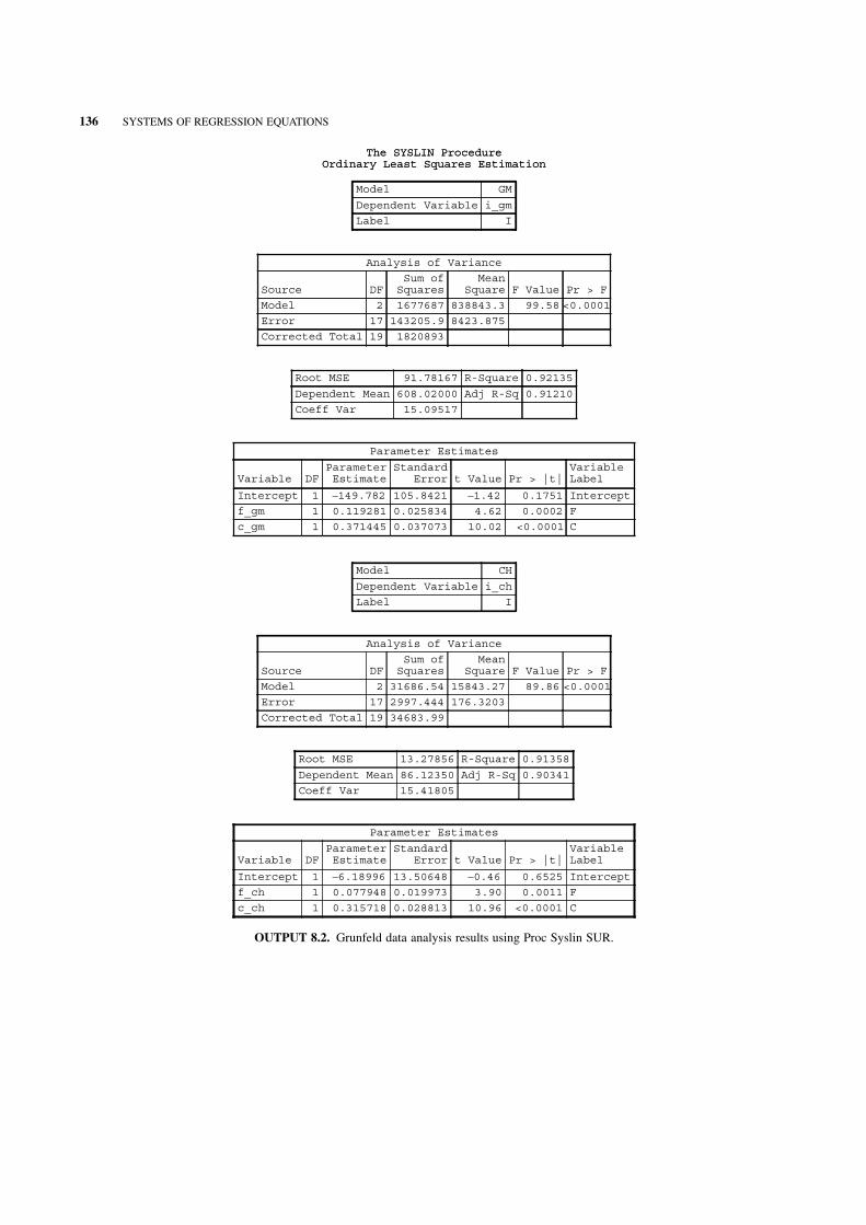
The SYSLIN ProcedureOrdinary Least Squares Estimation
The SYSLIN ProcedureOrdinary Least Squares Estimation
Model GM
Dependent Variable i_gm
Label I
Analysis of Variance
Source DFSum ofSquares
MeanSquare F Value Pr > F
Model 2 1677687 838843.3 99.58 <0.0001
Error 17 143205.9 8423.875
Corrected Total 19 1820893
Root MSE 91.78167 R-Square 0.92135
Dependent Mean 608.02000 Adj R-Sq 0.91210
Coeff Var 15.09517
Parameter Estimates
Variable DFParameterEstimate
StandardError t Value Pr > |t|
VariableLabel
Intercept 1 –149.782 105.8421 –1.42 0.1751 Intercept
f_gm 1 0.119281 0.025834 4.62 0.0002 F
c_gm 1 0.371445 0.037073 10.02 <0.0001 C
Model CH
Dependent Variable i_ch
Label I
Analysis of Variance
Source DFSum ofSquares
MeanSquare F Value Pr > F
Model 2 31686.54 15843.27 89.86 <0.0001
Error 17 2997.444 176.3203
Corrected Total 19 34683.99
Root MSE 13.27856 R-Square 0.91358
Dependent Mean 86.12350 Adj R-Sq 0.90341
Coeff Var 15.41805
Parameter Estimates
Variable DFParameterEstimate
StandardError t Value Pr > |t|
VariableLabel
Intercept 1 –6.18996 13.50648 –0.46 0.6525 Intercept
f_ch 1 0.077948 0.019973 3.90 0.0011 F
c_ch 1 0.315718 0.028813 10.96 <0.0001 C
OUTPUT 8.2. Grunfeld data analysis results using Proc Syslin SUR.
136 SYSTEMS OF REGRESSION EQUATIONS

The SYSLIN ProcedureOrdinary Least Squares Estimation
The SYSLIN ProcedureOrdinary Least Squares Estimation
Model GE
Dependent Variable i_ge
Label I
Analysis of Variance
Source DFSum ofSquares
MeanSquare F Value Pr > F
Model 2 31632.03 15816.02 20.34 <0.0001
Error 17 13216.59 777.4463
Corrected Total 19 44848.62
Root MSE 27.88272 R-Square 0.70531
Dependent Mean 102.29000 Adj R-Sq 0.67064
Coeff Var 27.25850
Parameter Estimates
Variable DFParameterEstimate
StandardError t Value Pr > |t|
VariableLabel
Intercept 1 –9.95631 31.37425 –0.32 0.7548 Intercept
f_ge 1 0.026551 0.015566 1.71 0.1063 F
c_ge 1 0.151694 0.025704 5.90 <0.0001 C
Model WE
Dependent Variable i_we
Label I
Analysis of Variance
Source DFSum ofSquares
MeanSquare F Value Pr > F
Model 2 5165.553 2582.776 24.76 <0.0001
Error 17 1773.234 104.3079
Corrected Total 19 6938.787
Root MSE 10.21312 R-Square 0.74445
Dependent Mean 42.89150 Adj R-Sq 0.71438
Coeff Var 23.81153
Parameter Estimates
Variable DFParameterEstimate
StandardError t Value Pr > |t|
VariableLabel
Intercept 1 –0.50939 8.015289 –0.06 0.9501 Intercept
f_we 1 0.052894 0.015707 3.37 0.0037 F
c_we 1 0.092406 0.056099 1.65 0.1179 C
OUTPUT 8.2. (Continued)
.
FEASIBLE GENERALIZED LEAST SQUARES 137

Model US
Dependent Variable i_us
Label I
Analysis of Variance
Source DFSum ofSquares
MeanSquare F Value Pr > F
Model 2 139978.1 69989.04 6.69 0.0072
Error 17 177928.3 10466.37
Corrected Total 19 317906.4
Root MSE 102.30529 R-Square 0.44031
Dependent Mean 405.46000 Adj R-Sq 0.37447
Coeff Var 25.23191
Parameter Estimates
Variable DFParameterEstimate
StandardError t Value Pr > |t|
VariableLabel
Intercept 1 –30.3685 157.0477 –0.19 0.8490 Intercept
f_us 1 0.156571 0.078886 1.98 0.0635 F
c_us 1 0.423866 0.155216 2.73 0.0142 C
The SYSLIN ProcedureSeemingly Unrelated Regression Estimation
The SYSLIN ProcedureSeemingly Unrelated Regression Estimation
Cross Model Covariance
GM CH GE WE US
GM 8423.88 –332.655 714.74 148.443 –2614.2
CH –332.65 176.320 –25.15 15.655 491.9
GE 714.74 –25.148 777.45 207.587 1064.6
WE 148.44 15.655 207.59 104.308 642.6
US –2614.19 491.857 1064.65 642.571 10466.4
Cross Model Correlation
GM CH GE WE US
GM 1.00000 –0.27295 0.27929 0.15836 –0.27841
CH –0.27295 1.00000 –0.06792 0.11544 0.36207
GE 0.27929 –0.06792 1.00000 0.72896 0.37323
WE 0.15836 0.11544 0.72896 1.00000 0.61499
US –0.27841 0.36207 0.37323 0.61499 1.00000
Cross Model Inverse Correlation
GM CH GE WE US
GM 1.41160 0.14649 –0.32667 –0.46056 0.74512
CH 0.14649 1.23373 0.27615 –0.08670 –0.45566
GE –0.32667 0.27615 2.33055 –1.65117 –0.04531
WE –0.46056 –0.08670 –1.65117 3.16367 –1.42618
US 0.74512 –0.45566 –0.04531 –1.42618 2.26642
OUTPUT 8.2. (Continued).
138 SYSTEMS OF REGRESSION EQUATIONS

The SYSLIN ProcedureSeemingly Unrelated Regression Estimation
Cross Model Inverse Covariance
GM CH GE WE US
GM 0.000168 0.000120 –0.000128–0.000491 0.000079
CH 0.000120 0.006997 0.000746 –0.000639–0.000335
GE –0.000128 0.000746 0.002998 –0.005798–0.000016
WE –0.000491–0.000639–0.005798 0.030330 –0.001365
US 0.000079 –0.000335–0.000016–0.001365 0.000217
System Weighted MSE 0.9401
Degrees of freedom 85
System Weighted R-Square 0.8707
Model GM
Dependent Variable i_gm
Label I
Parameter Estimates
Variable DFParameterEstimate
StandardError t Value Pr > |t|
VariableLabel
Intercept 1 –162.364 97.03216 –1.67 0.1126 Intercept
f_gm 1 0.120493 0.023460 5.14 <0.0001 F
c_gm 1 0.382746 0.035542 10.77 <0.0001 C
Model CH
Dependent Variable i_ch
Label I
Parameter Estimates
Variable DFParameterEstimate
StandardError t Value Pr > |t|
VariableLabel
Intercept 1 0.504304 12.48742 0.04 0.9683 Intercept
f_ch 1 0.069546 0.018328 3.79 0.0014 F
c_ch 1 0.308545 0.028053 11.00 <0.0001 C
Model GE
Dependent Variable i_ge
Label I
Parameter Estimates
Variable DFParameterEstimate
StandardError t Value Pr > |t|
VariableLabel
Intercept 1 –22.4389 27.67879 –0.81 0.4287 Intercept
f_ge 1 0.037291 0.013301 2.80 0.0122 F
c_ge 1 0.130783 0.023916 5.47 <0.0001 C
Model WE
Dependent Variable i_we
Label I
OUTPUT 8.2. (Continued).
FEASIBLE GENERALIZED LEAST SQUARES 139

ge:model i_ge = f_ge c_ge;
we:model i_we = f_we c_we;
us:model i_us = f_us c_us;
run;
The first part of the output gives theOLS equation-by-equation estimates of the parameters for each of the five firms. Notice
that the F test for the global hypothesisH0: b1¼b2¼b3¼ 0 versusH1: At least one b 6¼ 0 is highly significant for each of the
five firms. The root MSE value is the highest for US and lowest for WE. The R2 values for GM and CH indicates a good fit,
while theR2 values GE andWE indicate amoderate fit. TheR2 value for US indicates a poor fit. Both explanatory variables are
highly significant for firms GM and CH. Market value is not significant in the model for GE, WE, and US at the 5%
significance level.
The OLS equation-by-equation output is followed by the cross-equation covariance and correlation matrices along with their
inverses. The diagonal elements of the cross-model covariance matrix are the variances of the residuals for the five firms. For
example, the variance of the residuals for GM is 8423.88. Taking the square root of this will yield 91.78, which is the rootMSE of
the OLS model for this firm. The off-diagonal elements of this matrix display the values of the covariances between the OLS
residuals of each of the five firms. The cross-equation covariance is calculated by first calculating the residuals
ðei; i ¼ 1; . . . ;M ¼ 5Þ from the FGLS procedure for each firm and each time period. Let
E ¼ e1 e2 e3 e4 e5½ �:
The covariance matrix is given by
1
TETE ðGreen; 2003; p: 322Þ;
where T in Grunfeld’s model example is 20.
The cross-equation correlation is calculated by using the formula
rðx; yÞ ¼ Covðx; yÞ=ðsxsyÞ:
This results in all diagonal elements being equal to 1. To see how the off-diagonal elements are calculated, consider calculating
the correlation between the residuals of firms GM and CH. Using this formula, one gets
rðGM;CHÞ ¼ �332:655.
ffiffiffiffiffiffiffiffiffiffiffiffiffiffiffiffi
8423:88p ffiffiffiffiffiffiffiffiffiffiffiffiffiffi
176:32p� �
¼ �0:273:
Parameter Estimates
Variable DFParameterEstimate
StandardError t Value Pr > |t|
VariableLabel
Intercept 1 1.088877 6.788627 0.16 0.8745 Intercept
f_we 1 0.057009 0.012324 4.63 0.0002 F
c_we 1 0.041506 0.044689 0.93 0.3660 C
Model US
Dependent Variable i_us
Label I
Parameter Estimates
Variable DFParameterEstimate
StandardError t Value Pr > |t|
VariableLabel
Intercept 1 85.42325 121.3481 0.70 0.4910 Intercept
f_us 1 0.101478 0.059421 1.71 0.1059 F
c_us 1 0.399991 0.138613 2.89 0.0103 C
OUTPUT 8.2. (Continued).
140 SYSTEMS OF REGRESSION EQUATIONS

The cross-equation correlation matrix indicates high correlation between the residuals of GE and WE, and WE and US. The
inverse of both the cross-equation covariance and correlation matrices wraps up this portion of the output.
The last part of the output consists of the FGLS estimates of the parameters of the two explanatory variables for each of the five
firms.Theoutputdisplaysboth the systemweightedMSEand the systemweightedR2.Note that thedegreesof freedomassociated
with the systemweightedMSE is 17� 5 ¼ 85. The analysis results indicate that bothmarket value and the value of stock of plant
and equipment are highly significant for firms GM, CH, and GE. The value of stock of plant and equipments is not significant for
firm WE. The market value is not significant for firm US.
FEASIBLE GENERALIZED LEAST SQUARES 141

9SIMULTANEOUS EQUATIONS
9.1 INTRODUCTION
Theprevious chapters focusedon single equations andon systemsof single equationmodels thatwere characterizedbydependent
variables (endogenous) on the left-hand side and the explanatory variables (exogenous or endogenous) on the right-hand side of
the equations. For example, Chapter 4 dealt with instrumental variables, where the endogenous variables were on the right-hand
side. This chapter extends the concept of systems of linear equations where endogenous variables were determined one at a time
(sequentially) to the case when they are determined simultaneously.
We begin our discussion of simultaneous equation models by considering the following wage–price equations
pt ¼ b1wt þ b2mt þ «1t
wt ¼ a1pt þ a2ut þ «2t;
wherept is the price inflation at time t,wt iswage inflation at time t,mt is themoney supply at time t,u1 is unemployment rate time t,
«1t and «2t are the error termswithmeans 0 and constant variancess21 ands
22, respectively, and g ¼ ðb1;b2;a1;a2Þ are themodel
parameters that need to be estimated.We also assume that the disturbance terms are uncorrelated. These equations are referred to
as structural equations. In the wage–price inflation equation, we have two structural equations and four unknown parameters.
The first equationdescribes the relationof price inflation towage inflation andmoney supply.Aswages increase so doprices as
demand forgoodand services tend to increase aswell and this puts pressure on them.Furthermore, the increase inwage is typically
passed on to the consumer resulting in price inflation. There is also a positive relationship between money supply and price
inflation. The second equation describes the behavior of wage inflation vis-a-vis price inflation and the unemployment rate. As
prices increase, workers tend to demand higher wages but the demand is offset by the unemployment rate since a higher
unemployment rate tends to decrease the rate ofwage increases as the demand of goods and services decreases and thus there is no
pressure on price.
Notice that both equations are required to determine the price and wage inflations. The variables p and w are therefore
endogenous variables. Theunemployment rate andmoney supply are determined outside of the systemof equations and therefore
exogenous.
9.2 PROBLEMS WITH OLS ESTIMATION
In this section, we will show why ordinary least squares estimation for simultaneous equations is inappropriate. Recall that a
critical assumption of OLS is that the explanatory variables are exogenous. This assumption is violated when an endogenous
142
Applied Econometrics Using the SAS� System, by Vivek B. AjmaniCopyright � 2009 John Wiley & Sons, Inc.

variable becomes an explanatory variable in another equation of the system. OLS estimates in this case will lead to biased and
inconsistent estimatiors. We will illustrate this by considering the first equation of the wage–price inflation system of
equations given above.
Consider the second equation in the wage–price inflation system. The expectation Eðwt«1tÞ is given by
Eðwt«1tÞ ¼ a1Eðpt«1tÞ þ a2Eðut«1tÞ þ Eð«2t«1tÞ:
Using the assumptions stated earlier, it can be shown that this simplifies to
Eðwt«1tÞ ¼ a1Eðpt«1tÞ
E pt«1tð Þ ¼1
a1
E wt«1tð Þ:
Taking the expectation Eðpt«1tÞ and substituting the above in it, we get
1
a1
E wt«1tð Þ ¼ b1E wt«1tð Þ þ a2E mt«1tð Þ þ E «21t� �
:
Using the earlier assumptions, we can show that
E wt«1tð Þ ¼a1
1�a1b1
s2 6¼ 0:
Therefore, wt is endogenous with respect to «1t and the OLS assumptions are violated. Using OLS, therefore, will lead to biased
and inconsistent estimators of the parameters in the first equation.
The nature of the bias can be shown by writing down the OLS estimate expression for b1
b1 ¼
P
T
t¼1
ðwt�w�Þðpt� p�Þ
P
T
t¼1
ðwt�w�Þ2:
Simplifying this, we get
b1 ¼ b1 þ b2
P
T
t¼1
ðwt�w�Þðmt�m�Þ
P
T
t¼1
ðwt�w�Þ2þ
P
T
t¼1
ðwt�w�Þð«t� «�Þ
P
T
t¼1
ðwt�w�Þ2:
Asymptotically, the second term is simply the covariance between wage and money flow and is assumed to be zero based
on the wage–price inflation structural equations. Asymptotically, the last expression gives the covariance between wage
and the disturbance of the first equation and is nonzero as shown earlier. The denominator term is the asymptotic
variance of wage. The OLS estimate is therefore biased and inconsistent with the direction of the bias depending on
Covðwt; «tÞ.Ashenfelter et al. (2003, pp. 222–223) use the simple Keynesian model
ct ¼ b0 þ b1yt þ «t
yt ¼ ct þ it
to show the nature of the bias of the OLS estimator for b1. Here, ct is the consumption at time t, yt is the income at time t, it is
investment at time t, «t is the disturbance with zero mean and variance s2«, and b ¼ ðb0;b1Þ are parameters to be estimated. The
PROBLEMS WITH OLS ESTIMATION 143

authors show that the OLS estimator of b1 is biased upwards and is given by
bias b1
� �
¼s2«
ð1�b1Þs2y
;
where
s2y ¼ VarðytÞ:
9.3 STRUCTURAL AND REDUCED FORM EQUATIONS
The wage–inflation system of equations given in Section 9.1 contains two structural equations in four unknown
parameters. The basic goal of simultaneous equation modeling is to provide estimates of the parameters in the structural
equations. A natural path to estimating these parameters can be seen by first expressing the endogenous variables in the
system of equations as functions of the exogenous variables in the system. The resulting equations are called reduced form
equations.
For thewage–price inflation structural equations, the reduced form equations can be obtained by substituting the equation for
wage in the equation for price and vice-versa, the equation of price in the equation forwage. To see how the reduced formequation
for price is constructed, consider
pt ¼ b1ða1pt þ a2ut þ «2tÞ þ b2mt þ «1t
pt ¼ a1b1pt þ a2b1ut þ b1«2t þ b2mt þ «1t
pt�a1b1pt ¼ a2b1ut þ b2mt þ b1«2t þ «1t
pt ¼a2b1
1�a1b1
ut þb2
1�a1b1
mt þb1«2t þ «1t
1�a1b1
:
Proceeding in a similar fashion, we can get the reduced form equation for wt. The reduced forms are given by
pt ¼b2
1�a1b1
mt þa2b1
1�a1b1
ut þ«1t þ b1«2t
1�a1b1
;
wt ¼a1b2
1�a1b1
mt þa2
1�a1b1
ut þa1«1t þ «2t
1�a1b1
:
The above approach for creating the reduced form equations from the structural equations should suggest an approach to
estimating the structural equation parameters. We could, in principle, conduct an OLS on the reduced form equations and
then attempt to extract the structural equation parameters from the reduced form parameters. Another option is to first run
OLS on the reduced form equations to get the predicted values of the endogenous variables. The predicted values of the
endogenous variables can then be used in an OLS in the structural equations to estimate the parameters of interest. We
will discuss estimation techniques in the next section. For now, we will move on to the system of equations in the more
general case.
As shown inGreene (2003, p. 382), thegeneral structure of the structural equations at time twithn endogenous and kexogenous
variables can be written as
a11yt1 þ . . . þ an1ytn þ b11xt1 þ . . .þ bk1xtk ¼ «t1
a12yt1 þ . . .þ an2ytn þ b12xt1 þ . . .þ bk2xtk ¼ «t2
.
.
.
a1nyt1 þ . . .þ annytn þ b1nxt1 þ . . .þ bknxtk ¼ «tn:
144 SIMULTANEOUS EQUATIONS

In matrix notation, the system of structural equations at time t can be written as yTt Gþ xTt B ¼ «Tt , where
yTt ¼ ½yt1; . . . ; ytn�;
G ¼
a11 a12 . . . a1n
a21 a22 . . . a2n
.
.
....
..
....
an1 an2 . . . ann
2
6
6
6
6
6
6
4
3
7
7
7
7
7
7
5
;
xTt ¼ ½xt1; . . . ; xtk�;
B ¼
b11 b12 . . . b1n
b21 b22 . . . b2n
.
.
....
..
....
bk1 bk2 . . . bkn
2
6
6
6
6
6
6
4
3
7
7
7
7
7
7
5
;and
«Tt ¼ ½«1; . . . ; «n�:
Here, G is a n� nmatrix of coefficients for the endogenous variables, yt is a n� 1 vector of endogenous variables, B is a k � n
matrix of coefficients of the exogenous variables, xt is a k � 1vector consisting of exogenous variables, and «t is a n� 1vector of
disturbances.
Assuming that G is nonsingular, we can express the endogenous variables in reduced form as a function of the exogenous
variables and the random disturbances. The reduced form system of equations at time period t is given by (Greene, 2003, p. 384)
yTt ¼ �xTt BG�1 þ «Tt G
�1
¼ xTt Pþ vTt ;
whereP is a k � nmatrix containing the parameters of the reduced form equations and vt contains the disturbances of the reduced
form equations
If we apply this to the wage–inflation model, we get
G ¼1 �a1
�b1 1
" #
; yt ¼pt
wt
" #
;
B ¼�b2 0
0 �a2
� �
; xt ¼mt
ut
� �
; and «t ¼«1t
«2t
� �
.
It is easily verified that the reduced form equation of the wage–inflation model at the tth observation is given by
½ pt wt � ¼ �½mt ut ��b2 0
0 �a2
" #
1
1�a1b1
a1
1�a1b1
b1
1�a1b1
1
1�a1b1
2
6
6
6
6
6
4
3
7
7
7
7
7
5
þ ½ «1t «2t �
1
1�a1b1
a1
1�a1b1
b1
1�a1b1
1
1�a1b1
2
6
6
6
6
6
4
3
7
7
7
7
7
5
;
which simplifies to the reduced form equations given earlier.
9.4 THE PROBLEM OF IDENTIFICATION
In the ideal case, wewould estimate the parameters of the reduced-form equation and then use these to estimate the parameters of
the structural-form equations. In most cases, however, the reduced form estimates do not provide direct estimates of the
parameters for the structural equation. It turns out that they only provide estimates of functions of the structural equation
THE PROBLEM OF IDENTIFICATION 145

parameters. The problem of identification deals with whether we can solve the reduced form equations for unique values of the
parameters of the structural equations.
To lay the groundwork for whether the structural equation parameters can be estimated, consider the wage–price inflation
system of equations. The reduced form parameters are
P11 ¼b2
1�a1b1
;
P12 ¼b1a2
1�a1b1
;
P21 ¼a1b2
1�a1b1
;
P22 ¼a2
1�a1b1
:
It should be obvious that the knowledge of the four reduced form parameters will allow us to estimate the four structural form
parameters. That is, the ratioP12=P22 givesusa2while the ratioP21=P11 givesusa1. Thevalues ofb1 andb2 canbe extracted in a
similarmanner.Here, we say that the structural equations are identified. In thewage–price inflation system,we have four reduced
form parameters and four structural parameters, and we could solve the reduced form parameter equations easily to extract the
structural equation parameters.
9.4.1 Determining if the Structural Equations are Identified
Consider the following simple two-equation model with two endogenous and two exogenous variables
y1 ¼ b0y2 þ b1x1 þ b2x2 þ «1;
y2 ¼ a0y1 þ a1x1 þ a2x2 þ «2:
It can be shown that the reduced form parameters are given by
P11 ¼b0a1 þ b1
1�b0a0
;
P12 ¼b0a2 þ b2
1�b0a0
;
P21 ¼b1a0 þ a1
1�b0a0
;
P22 ¼b2a0 þ a2
1�b0a0
:
It should be obvious that the knowledge of the four reduced form parameters will not allow us to estimate the six structural
equation parameters. However, assume that b2 is 0. In this case, we can easily show that
b0 ¼ P12=P22;
b1 ¼ P11�P12
P22
P21:
Similarly, if we assume that a2 ¼ 0, then it can be shown that
a0 ¼ P22=P12;
a1 ¼ P21�P22
P12
P11:
146 SIMULTANEOUS EQUATIONS

In the first case, we say that the structural equation for y1 is identified and in the second that the structural equation for y2 is
identified.
It should therefore be clear that one approach to estimating the structural equation parameters is to put restrictions on the
structural equations. In the example used, both structural equationswere identified by eliminating the exogenous variable x2. This
methodology can be formalized.
When no restrictionswere placed on the structural parameters of the above equations, the equationswere not identified. In this
case, no exogenous variables were removed and both structural equations had one endogenous variable on the right-hand side.
When one exogenous variable was removed from the structural equations, we were able to estimate the structural equations.
In general, if we let k be the number of excluded exogenous variables in the structural equation and let m be the number of
included endogenous variables in the structural equation, then the structural equation is identified if k ¼ m. On the other hand, the
structural equation is not identified if k < m. See Ashenfelter et al. (2003, pp. 223–226) for a good discussion of this. Greene
(2003, pp. 390–392) extends this to the general case.
9.5 ESTIMATION OF SIMULTANEOUS EQUATION MODELS
The two-stage least squares method is the most commonly used method for estimating parameters in a simultaneous equation
system. The approach involves first using OLS to estimate the reduced form equations. The predicted values of the endogenous
variables are then used in an OLS regression of the identified structural form equation of interest to estimate the parameters.
Abrief description of themethod is summarized here. First, recall that each structural equation iswritten so that an endogenous
variable on the left-hand sideof the equation is expressedas a functionof endogenousvariables and the exogenousvariables on the
right-hand side of the equation. Thus, for a system with n equations, there are n endogenous variables. If we let yj represent the
endogenous variable for the j th equation, then we can write the structural equation as
yj ¼ Y*j aj þ Xjbj þ «j j ¼ 1; . . . ; n:
Here,Y*j is aT � njmatrix of nj included endogenous variables on the right hand,aj is a nj � 1vector of coefficients forY*
j ,Xj is a
T � k*j matrix of included exogenous variables,bj is the kj � 1vector of coefficients forXj; and «j is the T � 1 disturbance vector.
Let, Wj ¼ ½Y*j Xj � and uj ¼ ½aj bj �, then the jth equation can be written as
yj ¼ Wjuj þ «j j ¼ 1; . . . ; n:
A naıve approach to analysis is to conduct an OLS of yj on Wj to get
uj ¼ ðWTj WjÞ
�1WT
j yj:
As shown earlier, OLS estimates are biased and inconsistent. Greene (2003, p. 396) gives an expression of theOLS estimates and
discusses the bias in the general setting.
The 2SLSmethod involves first conducting anOLS of the included endogenous variablesY*j on all the exogenous variables in
the system of equations. If we denote the predicted values of Y*j as Y
*j , then the 2SLS estimator is given by
u;IV ; j ¼ ðWTj WjÞ
�1WT
j yj;
where Wj ¼ bY^ *j Xj c . The asymptotic variance–covariance matrix for the 2SLS estimator is given by
Varðu^IV ; jÞ ¼ sjbWTj Wjc;
where
sj ¼ðyj�WjuIV ; jÞ
Tðyj�WjuIV ; jÞ
T:
See Greene (2003, pp. 398–399) for details.
ESTIMATION OF SIMULTANEOUS EQUATION MODELS 147

We will illustrate computing the 2SLS estimators for a labor–wage equation. Ashenfelter et al. (2003, p. 233) gives a
simultaneous system consisting of two equations, one for labor and one for wages, for the US agricultural labor market. The
authors provide the equations and a description of the variables list that is summarized below.
lnðLiÞ ¼ b0 þ b1lnðWiÞ þ b2lnðLandiÞ þ b3lnðREiÞ þ b4lnðOthexpiÞ þ b5lnðSchiÞ þ «1
lnðWiÞ ¼ a0 þ a1lnðLiÞ þ a2lnðSchiÞ þ a3lnðOthwagiÞ þ «2:
Here, L ¼ farm labor by state as measured by total number of worked days,W=wages per hour of farm workers, RE = research
anddevelopment expenses,Land= value of farmlandcapital,Othexp= operating expenses besides labor,Sch=median number of
years of formal schoolingofmales, andOthwag=weightedaverageofwages for nonfarmworkers.Note that thevariablesLandW
are endogenous while the other variables are exogenous. It is easy to show that the labor equation is exactly identified while the
wage equation is overidentified.
The following statements can be used to conduct an OLS regression on the labor equation.
data SE;
set SE;
L=log(labor);
W=log(wage);
L_re=Log(RE);
L_Land=log(land);
L_Othexp=log(othexp);
L_Sch=log(sch);
L_Othwag=Log(othwag);
run;
proc reg data=SE;
model L=W L_Land L_re L_Othexp L_Sch;
run;
Output 9.1 contains the analysis of the data using standardOLS. Recall that OLS gives biased and inconsistent estimators of the
structural model parameters. Notice that the parameters for wages, value of land, R&D expenditure, and other nonlabor expense
are highly significant. The coefficient for schooling is not significant. The sign for thewages coefficient makes intuitive sense. As
wages increase, employers cut back on labor and therefore the number of labor days should decrease.
The following statements can be used to estimate the labor equation by the 2SLS method. The analysis results are given in
Output 9.2. There are fourmain statements in the Proc Syslin procedure as it relates to the labor equation. First, the option 2SLS is
used to request the two-stage instrumental variable estimator. Second, the endogenous statement lists out the two endogenous
variables in the system. Next, we list out the instruments that will be used in the estimation. This is followed by the model
statement.
proc syslin data=SE 2SLS;
endogenous L W;
instruments L_land L_RE L_Othexp L_Sch L_Othwag;
Labor: model L = W L_Land L_RE L_Othexp L_Sch;
run;
The analysis indicates that the global F test for the model is significant (p value < 0:001). The value of the statistic is veryclose to the one obtained byOLS. Aswe saw in theOLS output, schooling is not significant whereas all the othermodel variables
are significant. However, the sign associated with schooling is positive compared to negative in the OLSmodel. The sign for the
intercept is also different while the other variables have the same sign as in the OLS model. The values of the coefficient of
determination and the root MSE are very close to what was obtained from OLS.
Since the model used is a log–log model, we can interpret the coefficients as follows (taking research and development as an
example): If the research and development expense increases by 10%, then farm labor increases by 0:10� 0:47 ¼ 0:047 ¼ 4:7%days.
The2SLSestimator isbasedon theassumptionofhomoscedasticdisturbances.White�s estimator for thevariancecovariancecan
beused if this assumption isviolated.The resultingestimator is called thegeneralizedmethodofmoments (GMM)estimator.To see
148 SIMULTANEOUS EQUATIONS

The REG ProcedureModel: MODEL1
Dependent Variable: L
Number of Observations Read 39
Number of Observations Used 39
Analysis of Variance
Source DFSum of
SquaresMean
Square F Value Pr > F
Model 5 11.01673 2.20335 45.12 <0.0001
Error 33 1.61160 0.04884
Corrected Total 38 12.62833
Root MSE 0.22099 R-Square 0.8724
Dependent Mean 10.29862 Adj R-Sq 0.8530
Coeff Var 2.14582
Parameter Estimates
Variable DFParameterEstimate
StandardError t Value Pr > |t|
Intercept 1 0.87573 1.94350 0.45 0.6552
W 1 -1.10577 0.28931 -3.82 0.0006
L_Land 1 0.31180 0.08373 3.72 0.0007
L_re 1 0.44460 0.11402 3.90 0.0004
L_Othexp 1 0.26454 0.11278 2.35 0.0252
L_Sch 1 -0.26232 0.60820 -0.43 0.6691
OUTPUT 9.1. OLS analysis of the labor equation.
The SYSLIN ProcedureTwo-Stage Least Squares Estimation
Model LABOR
Dependent Variable L
Analysis of Variance
Source DFSum ofSquares
MeanSquare F Value Pr > F
Model 5 10.59918 2.119837 41.63 <0.0001
Error 33 1.680444 0.050923
Corrected Total 38 12.62833
Root MSE 0.22566 R-Square 0.86315
Dependent Mean 10.29862 Adj R-Sq 0.84242
Coeff Var 2.19117
Parameter Estimates
Variable DFParameterEstimate
StandardError t Value Pr > |t|
Intercept 1 -0.85913 3.306459 -0.26 0.7966
W 1 -1.44928 0.601228 -2.41 0.0217
L_Land 1 0.328677 0.089282 3.68 0.0008
L_re 1 0.468702 0.122089 3.84 0.0005
L_Othexp 1 0.249787 0.117341 2.13 0.0408
L_Sch 1 0.342098 1.111155 0.31 0.7601
OUTPUT 9.2. 2SLS analysis of the labor equation.
ESTIMATION OF SIMULTANEOUS EQUATION MODELS 149

the construction of this estimator, first note that the 2SLS estimator can be written as (Greene, 2003, p. 399)
u IV; j ¼ ½ðWTj XÞðX
TXÞ�1ðXTWjÞ��1ðWT
j XÞðXTXÞ�1
XTyj;
where ðXTXÞ is called the weight matrix. Replacing this with White�s estimator
S0; j ¼X
T
t¼1
xtxTt ðyjt�wT
jt u IV; jÞ2
The MODEL Procedure
Model Summary
Model Variables 6
Endogenous 1
Exogenous 4
Parameters 6
Equations 1
Number of Statements 1
Model Variables L W L_Land L_re L_Othexp L_Sch
Parameters b0 b1 b2 b3 b4 b5
Equations L
The Equation to Estimate is
L = F(b0(1), b1(W), b2(L_Land), b3(L_re), b4(L_Othexp), b5(L_Sch))
Instruments 1 L_Land L_re L_Othexp L_Sch L_Othwag
NOTE: At GMM Iteration 0 convergence assumed because OBJECTIVE=1.095301E-24 is almost zero (<1E-12).
The MODEL ProcedureGMM Estimation Summary
Data SetOptions
DATA= SE
Minimization Summary
Parameters Estimated 6
Kernel Used PARZEN
l(n) 2.080717
Method Gauss
Iterations 0
Final ConvergenceCriteria
R 1
PPC 5.23E-12
RPC .
Object .
Trace(S) 0.050923
Objective Value 1.1E-24
ObservationsProcessed
Read 39
Solved 39
OUTPUT 9.3. GMM estimators for the labor equation.
150 SIMULTANEOUS EQUATIONS

gives the GMM estimator (Greene, 2003, p. 401). Notice the similarity in the construction ofWhite�s estimator to the one used in
Chapter5.Also,notice theGMMestimator is constructed in three steps.First, a 2SLSisused toget u IV; j. In the second step,White�s
estimator is calculated. In the third step, this is used as a weight matrix to calculate the robust 2SLS estimator.
Wewill illustrate this method on the labor equation.Wewill use ProcModel to estimate the GMM estimator since Proc Syslin
does not have the option to perform aGMManalysis. The followingSAScode can be used. The analysis results are given inOutput
9.3. The procedure statements start off with specifying the model. Note the coefficient names are not unique and can be changed.
However, the variable names have to be identical to the ones used in the data set. Next, we specify the endogenous and exogenous
variables. These are then followed by specifying the instrument variables and requesting a model using GMM estimation. Proc
Model can fit the OLS and the 2SLS models. We used Proc Reg and Proc Syslin to minimize the output that is produced by using
Proc Model. Notice that the parameter estimates and the model diagnostic statistics are very similar to the ones from 2SLS
estimation.
Proc Model
L=b0+b1*W+b2*L_Land+b3*L_RE+b4*L_Othexp+b5*L_Sch;
Endogenous W;
Exogenous L_Land L_RE L_Othexp L_Sch;
Instruments L_Land L_RE L_Othexp L_Sch L_OTHWAG;
Fit L/GMM;
Run;
9.6 HAUSMAN’S SPECIFICATION TEST
Hausman�s specification test can be used to test whether an included exogenous variable in a simultaneous equation is
endogenous. As with all specification tests by Hausman we used in Chapters 4 and 7, this test compares two estimators, both of
which are consistent under the null hypothesis of exogeneity but only one is consistent under alternative hypothesis of
endogeneity.
Details of the Hausman�s specification test as it applies to simultaneous equation models can be found in Greene (2003,
pp. 413–415). The analysis can easily be done in SAS by using the ProcModel procedure. The following statements (labor–wage
The MODEL Procedure
Nonlinear GMM Summary of Residual Errors
EquationDF
ModelDF
Error SSE MSE Root MSE R-SquareAdjR-Sq
L 6 33 1.6804 0.0509 0.2257 0.8669 0.8468
Nonlinear GMM Parameter Estimates
Parameter Estimate
ApproxStdErr t Value
ApproxPr > |t|
b0 -0.85913 3.1700 -0.27 0.7881
b1 -1.44928 0.5905 -2.45 0.0196
b2 0.328677 0.0904 3.64 0.0009
b3 0.468702 0.1092 4.29 0.0001
b4 0.249787 0.1332 1.88 0.0696
b5 0.342098 1.2268 0.28 0.7821
Number ofObservations Statistics for System
Used 39 Objective 1.095E-24
Missing 0 Objective*N 4.272E-23
OUTPUT 9.3. (Continued)
HAUSMAN’S SPECIFICATION TEST 151

data being used) can be used to conduct the Hausman�s specification test comparing the OLS estimates with the 2SLS estimates.
Wedidnot include theoutput for the test as theOLSand2SLSoutputswere alreadyprovided.Thepvalue for the test is around0.90
and indicates that there is no gain in using the 2SLS model over the OLS model.
proc model data=SE;
L = b0+b1*W+b2*L_Land+b3*L_RE+b4*L_Othexp+b5*L_Sch;
W = a0+a1*L+a2*L_Sch+a3*L_Othwag;
ENDOGENOUS L W;
EXOGENOUS L_land L_RE L_Othexp L_Sch L_Othwag;
fit L/ols 2sls hausman;;
instruments L_land L_RE L_Othexp L_Sch L_Othwag;
run;
152 SIMULTANEOUS EQUATIONS

10DISCRETE CHOICE MODELS
10.1 INTRODUCTION
The preceding chapters were focused on discussion of modeling techniques where the responses were continuous. In practice,
we often encounter responses that are discrete. For example, direct marketing companies often model the response behavior of
consumers receiving an offer to buy their products. Here, y, the response variable, equals 1 if the consumer responds to the mail
offer, and it equals 0 otherwise. Direct marketing companies also build conversion models where again the response variable
equals 1 if the consumer’s inquiry about a mail offer results in a sale; the response variable equals 0 otherwise. Another example
involves attritionmodels built by insurance companies that predict the likelihood that an existing consumer will cancel his or her
policy to take up anewpolicywith a competitor.Here, the responsevariable equals 1 if the consumer cancels a policy, and it equals
0 otherwise. Attrition models can also be built by using duration models but the common approach in industry is to treat the
attrition response as 0 or 1.Acommon theme in each example is the binary nature of the responsevariable.Of course, the response
variable canassumemore than twodiscretevalues.This chapter dealswith estimatingparameters ofmodelswhere thedistribution
of the response variable is not continuous but discrete. We will focus our attention on logistic regression with dichotomous
responses, and Poisson regression.
By definition, the set of plausible values of a discrete random variable can be placed in a 1:1 correspondence with a finite or a
countable infinite set. Some examples of discrete random variables are as follows:
1. The number of customers walking into a bank between 12 noon and 1 P. M. Here, the response variable can assume values
0, 1, 2, . . ..
2. The response of a consumer to amailed offer for a newcredit card or auto insurance.Here, the responsevariable can assume
one of two possible values: 1, response; 0, no response.
3. Theviews on abortion of an individual can bemeasured as 1, strongly agree; 2, agree; 3, neutral; 4, disagree; and 5, strongly
disagree. Here, the response variable is ordinal as the values have a natural rank.
4. Themode of transportation chosen by a commuter. The choices can be classified as 1, drive; 2, ride-share; 3, bus; and so on.
Here, the values cannot be ordered, and therefore the random variable is called a discrete nominal variable.
5. A consumer’s choice of a fast-food restaurant among several available brand names. This is similar to the example
presented in (4).
153
Applied Econometrics Using the SAS� System, by Vivek B. AjmaniCopyright � 2009 John Wiley & Sons, Inc.
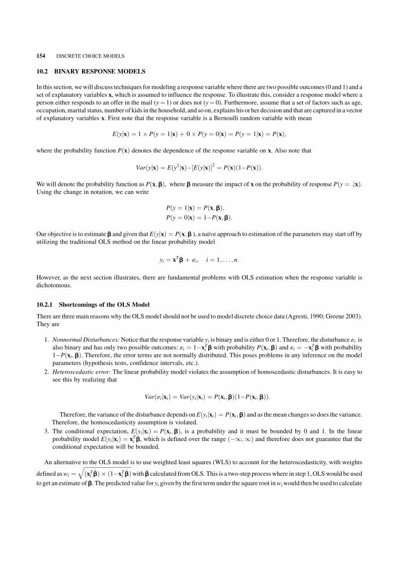
10.2 BINARY RESPONSE MODELS
In this section, wewill discuss techniques formodeling a response variablewhere there are two possible outcomes (0 and 1) and a
set of explanatory variables x, which is assumed to influence the response. To illustrate this, consider a response model where a
person either responds to an offer in the mail (y¼ 1) or does not (y¼ 0). Furthermore, assume that a set of factors such as age,
occupation,marital status, number of kids in the household, and so on, explains his or her decision and that are captured in avector
of explanatory variables x. First note that the response variable is a Bernoulli random variable with mean
EðyjxÞ ¼ 1� Pðy ¼ 1jxÞ þ 0� Pðy ¼ 0jxÞ ¼ Pðy ¼ 1jxÞ ¼ PðxÞ;
where the probability function PðxÞ denotes the dependence of the response variable on x. Also note that
VarðyjxÞ ¼ Eðy2jxÞ�½EðyjxÞ�2 ¼ PðxÞð1�PðxÞÞ:
Wewill denote the probability function as Pðx;bÞ, where bmeasure the impact of x on the probability of response Pðy ¼ :jxÞ.Using the change in notation, we can write
Pðy ¼ 1jxÞ ¼ Pðx;bÞ;
Pðy ¼ 0jxÞ ¼ 1�Pðx;bÞ:
Our objective is to estimate b and given that EðyjxÞ ¼ Pðx;b ), a naıve approach to estimation of the parameters may start off by
utilizing the traditional OLS method on the linear probability model
yi ¼ xTb þ «i; i ¼ 1; . . . ; n:
However, as the next section illustrates, there are fundamental problems with OLS estimation when the response variable is
dichotomous.
10.2.1 Shortcomings of the OLS Model
There are threemain reasons why the OLSmodel should not be used tomodel discrete choice data (Agresti, 1990; Greene 2003).
They are
1. Nonnormal Disturbances:Notice that the response variable yi is binary and is either 0 or 1. Therefore, the disturbance «i is
also binary and has only two possible outcomes: «i ¼ 1�xTi b with probability Pðxi;bÞ and «i ¼ �xTi b with probability
1�Pðxi;bÞ. Therefore, the error terms are not normally distributed. This poses problems in any inference on the model
parameters (hypothesis tests, confidence intervals, etc.).
2. Heteroscedastic error: The linear probability model violates the assumption of homoscedastic disturbances. It is easy to
see this by realizing that
Varð«ijxiÞ ¼ VarðyijxiÞ ¼ Pðxi;bÞð1�Pðxi;bÞÞ:
Therefore, the variance of the disturbance depends onEðyijxiÞ ¼ Pðxi;bÞ and as themean changes so does the variance.
Therefore, the homoscedasticity assumption is violated.
3. The conditional expectation, EðyijxiÞ ¼ Pðxi;bÞ, is a probability and it must be bounded by 0 and 1. In the linear
probability model EðyijxiÞ ¼ xTi b, which is defined over the range ð�1;1Þ and therefore does not guarantee that the
conditional expectation will be bounded.
An alternative to the OLS model is to use weighted least squares (WLS) to account for the heteroscedasticity, with weights
defined aswi ¼ffiffiffiffiffiffiffiffiffiffiffiffiffiffiffiffiffiffiffiffiffiffiffiffiffiffiffiffiffiffiffiffiffiffiffi
ðxTi bÞ � ð1�xTi bÞq
with b calculated fromOLS. This is a two-step process where in step 1, OLSwould be used
to get an estimate ofb. The predicted value for yi given by the first term under the square root inwiwould then be used to calculate
154 DISCRETE CHOICE MODELS

theweights for each observation. Theweights would then be used in step 2 to estimateb. TheWLSmodel thus becomes (Chapter
5, Myers, 1990, p. 316)
yi
wi
¼xTiwi
� �
b þ«i
wi
or y*i ¼ x*Ti b þ «*i :
The WLS would ensure homoscedasticity but would not ensure that the conditional mean xTi b is bounded by [0,1].
Estimation of b involving more efficient techniques exist and will now be discussed. Specifically, we will transform the
conditional mean by assuming either the probit or the logit distribution of the probability function Pðx;bÞ.
10.2.2 The Probit and Logit Models
As shown inAgresti (1990), by assuming a continuous distribution forPðx;bÞ, the conditional expectation xTi b can be bounded inthe interval ½0; 1�. There are two distributions that are commonly used: the normal and the logistic distribution.
If Pðx;bÞ is taken to be the cumulative standard normal distribution, then the resulting model is a probit model. That is,
Pðx;bÞ ¼ FðxTbÞ;
where FðtÞ ¼Ð
t
�1
f ðsÞdswith f ðsÞ being the probability density function of the standard normal distribution.
If
Pðx;bÞ ¼ex
Tb
1 þ exTb
¼ GðxTbÞ
then we have the logit model where GðxÞ is the logistic cumulative function given by
GðxÞ ¼expðxÞ
1 þ expðxÞ¼
1
1 þ expð�xÞ:
It is trivial to see that in both cases,Pðx;bÞ is bounded in the interval [0,1]. Agresti (1990, p. 105) discusses the complementary
log–logmodel as another alternative tomodeling binary responsevariables.However, the probit and logit distributions are the two
most commonly used to model binary response variables and we therefore focus on estimation techniques involving these two
distributions.
Notice that estimation usingmaximum likelihoodmethods will have to be used since the parameterb is now no longer a linear
function of Pðx;bÞ. The standard approach is to use the OLS estimates as the initial values for the MLE and then to iterate until
convergence.
10.2.3 Interpretation of Parameters
Asdiscussed inWooldridge (2002, p. 458), proper interpretationof themodel parameters for theProbit andLogitmodels is crucial
for successful implementation of the model. To see this, consider the formulation of the probit model where Pðx;bÞ ¼ FðxTbÞwhere FðxTbÞ is the cumulative normal distribution. Taking derivatives of this with respect to x we get (Greene, 2003, p. 667)
qPðx;bÞ
qx¼
qFðxTbÞ
qðxTbÞb ¼ f ðxTbÞb
where f ð*Þ is the normal probability density function. Therefore, themarginal effects depend on x via the density function. It can
be shown that the derivative of the conditional expectation for the logit model is given by
qPðx;bÞ
qx¼ GðxTbÞ½1�GðxTbÞ�b:
BINARY RESPONSE MODELS 155

Thus, the interpretation ofbmust be based on calculations done at a prespecified value of the explanatory variables x. A common
approach is to interpret themodel parameters at themean, �x. If a variable in x contains a dummy variable, then themarginal effect
of the variable can be computed as (Greene, 2003, p. 668; Wooldridge, 2002, p. 459)
Pðy ¼ 1j�xð�dÞ; xd ¼ 1Þ�Pðy ¼ 0j�xð�dÞ; xd ¼ 0Þ
where xd denotes that the explanatory variables contains a dummy variable and �xðdÞ is themeanvector of the other variables in the
model.
10.2.4 Estimation and Inference
Themethod ofmaximum likelihood is used to estimate the parameters because both the Probit and the Logitmodels are nonlinear
inb. To start our discussion ofmodel estimation, assume that we have an independent random sample ðyi; xiÞ;where i ¼ 1; . . . ; n
from the Bernoulli distribution with probability Pðxi;bÞ. Recall that the probability density function of a Bernoulli random
variable, x, is given by f ðxÞ ¼ pxð1�pÞ1�x, where x ¼ 0; 1, and p is the probability of success. Collecting all n observations and
assuming independence gives the likelihood function
Lðbjy;XÞ ¼Y
n
i¼1
Prðyijxi;bÞ;
¼Y
n
i¼1
Prðyi ¼ 0jxi;bÞ1�yiPrðyi ¼ 1jxi;bÞ
yi;
¼Y
n
i¼1
½1�Pðxi;bÞ�1�yi ½Pðxi;bÞ�
yi:
Taking the log of L ¼ Lðbjy;XÞ yields
lnðLÞ ¼X
n
i¼1
fyi ln Pðxi;bÞ þ ð1�yiÞ ln ½1�Pðxi;bÞ�g:
It can easily be shown that the log-likelihoods for the probit and logit models are as follows:
lnðLÞ ¼X
n
i¼1
fyi lnFðxTi bÞ þ ð1�yiÞ ln ½1�FðxTi bÞ�g for the Probit model; and
lnðLÞ ¼X
n
i¼1
fyi lnGðxTi bÞ þ ð1�yiÞ ln ½1�GðxTi bÞ�g for the Logit model:
The maximum likelihood parameters are found by taking the derivative of the log-likelihood equations, setting them to
zero and then solving for the unknown parameters. The first-order conditions are given by
LðbÞ ¼X
n
i¼1
yipi
Pi
þ ð1�yiÞ�pi
1�Pi
� �
xi:
where pi is the derivative of Pi with respect to xi.
Extending this to the Probit model, we get
LðbÞ ¼X
n
i¼1
yi �FðxTi bÞ
FðxTi bÞ � 1�FðxTi bÞ½ �fðxTi bÞxi;
156 DISCRETE CHOICE MODELS

whereas for the Logit model we have
LðbÞ ¼X
n
i¼1
yi �exp xTi b
� �
1 þ exp xTi bð Þ
2
4
3
5xi
As shown in Greene (2003, p. 671), it can be shown that the first-order condition for the Logit model can be written as
LðbÞ ¼X
n
i¼1
ðyi�GiÞxi ¼ 0:
The Hessian (second-order condition) for the Logit model is given by
H ¼q ln L
qbqbT¼ �
X
n
i¼1
Gið1�GiÞxi xTi :
The Newton–Raphson method is used to obtain a solution for these likelihood equations. The Hessian calculated in the final
iteration is the estimated covariance matrix of the coefficient vector.
10.2.5 The Newton–Raphson Method for the Logit Model
TheNewton–Raphson algorithm to obtain a solution for the likelihood equation of the Logitmodel can be summarized as follows
(Agresti, 1990):
1. Start with an initial set of estimates, bt¼0. Most often, the starting values are simply the OLS estimates. Here, t ¼ 0 simply
denotes the starting point.
2. Calculate the estimated value of the coefficient vector at time t þ 1 as given by bt þ 1 ¼ bt�H�1t gt, where gt is the gradient
vector defined as gt ¼ yi�Gt and Ht is the Hessian matrix. Here, Gt is the predicted probability of time t.
3. Iterate until the convergence criteria is reached. That is, until the difference of consecutive b values are insignificant.
We will now illustrate the Newton–Raphson algorithm to calculate the parameters (assuming a Logit model) for an
unemployment data set arising from a sample of 4877 blue collar workers who lost their jobs in the United States between
1982 and 1991 (McCall, 1995). All individuals in this study is assumed to have applied for unemployment benefits. Note that this
datawas also analyzed byVerbeek (2004, pp. 197–199). A description of the variableswas given by the author and is summarized
here. The variables in the data are as follows:
Y is the response variable and takes a value of 1 if the unemployed worker received unemployment benefits.
Age is the age of the subject.
Age2 is the square of the Age variable.
Tenure is the years of tenure at the last job.
Slack is an indicator variable that equals 1 if the subject was fired because of poor performance.
Abol is an indicator variable that equals 1 if the subject’s position was eliminated.
Seasonal is an indicator variable that equals 1 if the subject was a temporary worker.
NWHITE is an indicator variable that equals 1 if the subject’s race is nonwhite.
School12 is an indicator variable that equals 1 if the subject has more than 12 years of education.
Male is an indicator variable that equals 1 if the subject is a male.
SMSA is an indicator variable that equals 1 if the subject lives in a SMSA.
Married is an indicator variable that equals 1 if the subject is married.
DKIDS is an indicator variable that equals 1 if the subject has kids.
DYKIDS is an indicator variable that equals 1 if the subject has young kids.
YRDISP records the year when the job was lost. Here, 1982¼ 1 and 1991¼ 10.
BINARY RESPONSE MODELS 157

RR is the replacement rate that is the ratio of the benefits received versus the last recorded weekly earnings.
RR2 is the square of RR.
Head is an indicator variable that equals 1 if the subject is the head of a household.
StateUR is the state unemployment rate.
StateMB is the maximum benefits available for a given state.
The following Proc IML code can be used.
* Read the data file and scale age squared. ;
libname in "C:\Temp";
data test;
set in.unemp;
age2=age2/10;
run;
proc iml;
* Read the data into matrices and calculate some constants. ;
use test;
read all var {’rr’ ’rr2’ ’age’ ’age2’ ’tenure’
’slack’ ’abol’ ’seasonal’ ’head’ ’married’ ’dkids’
’dykids’ ’smsa’ ’nwhite’ ’yrdispl’ ’school12’ ’male’
’stateur’ ’statemb’} into X;
read all var {’y’} into Y;
n=nrow(X);
X=J(n,1,1)||X;
c=ncol(X);
* Calculate an initial estimate of the parameter vector. ;
Beta=inv(X‘*X)*X‘*y;
* Start the Newton-Raphson procedure. ;
Col_One=J(4877,1,1);
do index=1 to 5;
PI=exp(X*Beta)/(1+exp(X*Beta));
Temp_PI=Col_One-PI;
Diag_PI=Diag(PI#Temp_PI);
COV=inv(X‘*Diag_PI*X);
Beta_New=Beta+COV*X‘*(Y-PI);
DIFF=sum(abs(BETA_NEW-BETA));
print DIFF;
if DIFF<0.00001 then
do;
print ’The estimates of the coefficients are:’;
print Beta_New;
SE=sqrt(vecdiag(COV));
print ’The estimated standard errors are:’;
print SE;
stop;
end;
beta=beta_new;
end;
run;
The analysis results are given inOutput 10.1. Notice that the test statistic value and the p values were not computed here. They
can be easily computed by incorporating additional statements in the code provided. Wewill discuss the methodology when we
interpret the output from Proc Logistic.
158 DISCRETE CHOICE MODELS

The following statements can be used to fit an OLS model. The analysis results are given in Output 10.2. Note that this is the
incorrectmethod of analyzing data andwe include it here simply for comparing the results to the results obtained by using logistic
regression.
proc reg data=test;
model y=rr rr2 age age2 tenure slack abol
seasonal head married dkids dykids smsa nwhite
yrdispl school12 male stateur statemb;
run;
The following statements canbe used to fit aLogitmodel to theunemployment data.Note that themodel statement contains the
option “event¼1” that forces the procedure tomodel the probability of a response. The option “descending” in the first line can be
used to achieve the same results. The analysis results are given in Output 10.3.
proc logistic data=test;
model y(event=’1’)=rr rr2 age age2 tenure slack abol
seasonal head married dkids dykids smsa nwhite
yrdispl school12 male stateur statemb;
run;
We will now provide details about the output produced by Proc Logistic.
The first table gives basic model information that includes the names of the data set and the response variable, the number of
levels of the response variable (here two since the response is binary), and type of model (logit), and the optimization technique
used by the program (Fisher’s scoring).
The next three tables give information on the number of observations in the data set and the number of observations that were
used to estimate the model. These numbers will be different if there are missing observations in the data set. The next table gives
the response profile. There are 1542 nonresponders and 3335 responders. Therefore, out of the total number of individuals in the
study, 3335 unemployed workers applied for and received unemployment insurance while the remaining 1542 applied for
unemployment insurance but did not receive insurance.
The parameter estimates and their standard errors are:
OUTPUT_TABLE
BETA SE
INTERCEPT –2.8005 0.6042
RR 3.0681 1.8682
RR2 –4.8906 2.3335
AGE 0.0677 0.0239
AGE2 –0.0597 0.0304
TENURE 0.0312 0.0066
SLACK 0.6248 0.0706
ABOL –0.0362 0.1178
SEASONAL 0.2709 0.1712
HEAD –0.2107 0.0812
MARRIED 0.2423 0.0794
DKIDS –0.1579 0.0862
DYKIDS 0.2059 0.0975
SMSA –0.1704 0.0698
NWHITE 0.0741 0.0930
YRDISPL –0.0637 0.0150
SCHOOL12 –0.0653 0.0824
MALE –0.1798 0.0875
STATEUR 0.0956 0.0159
STATEMB 0.0060 0.0010
OUTPUT 10.1. Proc IML output for the logistic model of unemployment data.
BINARY RESPONSE MODELS 159

The Model Fit Statistics table gives three statistics that can be used to assess the fit of the model. The first column gives the
model fit statistics for themodelwith only the intercept termwhile the secondcolumnadjusts thevalues to account for the addition
of explanatory variables to the model. Smaller values of all three statistics are desirable.
The next table contains the chi-square test statistic value and the corresponding p value for the Global Null Hypothesis that
none of the coefficients in themodel are significant versus the alternative that at least one of the coefficients is significant. The chi-
squarevalue for the likelihood ratio is simply the difference between the log-likelihoodvalues from theprevious table. That is, it is
computed by taking the difference 6086.056� 5746.393¼ 339.663. The p value indicates that the overall model is highly
significant.
The REG ProcedureModel: MODEL1
Dependent Variable: y
Number of Observations Read 4877
Number of Observations Used 4877
Analysis of Variance
Source DFSum of
SquaresMean
Square F Value Pr > F
Model 19 70.55319 3.71333 18.33 <0.0001
Error 4857 983.90037 0.20257
Corrected Total 4876 1054.45356
Root MSE 0.45008 R-Square 0.0669
Dependent Mean 0.68382 Adj R-Sq 0.0633
Coeff Var 65.81857
Parameter Estimates
Variable DFParameterEstimate
StandardError t Value Pr > |t|
Intercept 1 –0.07687 0.12206 –0.63 0.5289
rr 1 0.62886 0.38421 1.64 0.1017
rr2 1 –1.01906 0.48095 –2.12 0.0342
age 1 0.01575 0.00478 3.29 0.0010
age2 1 –0.01459 0.00602 –2.43 0.0153
tenure 1 0.00565 0.00122 4.65 <0.0001
slack 1 0.12813 0.01422 9.01 <0.0001
abol 1 –0.00652 0.02483 –0.26 0.7928
seasonal 1 0.05787 0.03580 1.62 0.1060
head 1 –0.04375 0.01664 –2.63 0.0086
married 1 0.04860 0.01613 3.01 0.0026
Parameter Estimates
Variable DFParameterEstimate
StandardError t Value Pr > |t|
dkids 1 –0.03051 0.01743 –1.75 0.0802
dykids 1 0.04291 0.01976 2.17 0.0299
smsa 1 –0.03520 0.01401 –2.51 0.0121
nwhite 1 0.01659 0.01871 0.89 0.3753
yrdispl 1 –0.01331 0.00307 –4.34 <0.0001
school12 1 –0.01404 0.01684 –0.83 0.4047
male 1 –0.03632 0.01781 –2.04 0.0415
stateur 1 0.01815 0.00308 5.88 <0.0001
statemb 1 0.00124 0.00020393 6.08 <0.0001
OUTPUT 10.2. Proc Reg output for the linear model of the unemployment data.
160 DISCRETE CHOICE MODELS

The next table gives the parameter estimates, their standard errors along with the individual chi-square values and the
associatedpvalue.TheWald’s chi-squared test statistic canbecomputedby taking the squareof the ratio of theparameter estimate
to its standard error. For example, the Wald’s chi-squared value for the age variable is given by
0:0677
0:0239
� �2
¼ 8:02:
This can easily be programmed into Proc IML and then the PROBCHI function can be used to calculate the p values.
There are several variables that are significant in the model. As an example of how to interpret the variables consider the two
statevariables and the slackvariable.All three are highly significant. The significance of the statevariables indicate that thehigher
the state’s unemployment rate and the higher the benefits allowed the more likely it is that an employed person will receive
unemployment benefits. The variable slack indicates that a person whose job was terminated because of poor performance will
have a higher likelihood of receiving employment benefits.
The next table gives the odds ratio estimates alongwith the corresponding 95% confidence intervals. The odds ratios are calcu-
latedbysimply exponentiating theparameter estimates.For instance, theodds ratio for thevariable slack is exp ð0:6248Þ ¼ 1:868.
This implies that a personwhowas fired for poor performance is 1.868 timesmore likely to receive unemployment benefits than a
personwho lost his or her job for some other reason (all other variables being held constant). The odds ratio formales indicates that
theyare0.893timesaslikelytogetunemploymentinsurancebenefits thanfemales.That is, their likelihoodofgettingunemployment
insurance benefits is lower than that of females.
The last table gives association of predicted probabilities and the observed responses. See the SAS 9.2 User’s guide for a
description of these statistics.
The LOGISTIC ProcedureThe LOGISTIC Procedure
Model Information
Data Set WORK.TEST
Response Variable y
Number of Response Levels 2
Model binary logit
Optimization Technique Fisher's scoring
Number of Observations Read 4877
Number of Observations Used 4877
Response Profile
OrderedValue y
TotalFrequency
1 0 1542
2 1 3335
Probability modeled is y=1.
Model Convergence Status
Convergence criterion (GCONV=1E-8) satisfied.
Model Fit Statistics
CriterionIntercept
Only
Interceptand
Covariates
AIC 6088.056 5786.393
SC 6094.548 5916.239
-2 Log L 6086.056 5746.393
OUTPUT 10.3. Logit model output for the unemployment data.
BINARY RESPONSE MODELS 161

The following statements can be used to fit a binary Probit model. The analysis results are given in Output 10.4.
proc logistic data=test;
model y(event=’1’)=rr rr2 age age2 tenure slack abol
seasonal head married dkids dykids smsa nwhite
yrdispl school12 male stateur statemb/l=Probit;
run;
Notice that the model statistics from the first few tables are very similar between the logit and probit models. The model
parameters also have consistent signs. However, the magnitude of the parameter estimates are different.
The parameter estimates from the Probit model can be used to calculate the predicted probability that a person will receive
unemployment insurance. For a given individual, the predicted probability of receiving unemployment insurance can be
calculated by using
FðxTi bÞ ¼ Fð�1:6999 þ 1:8633rr�2:9801rr2 þ � � � þ 0:00364 statembÞ;
whereFðÞ is the cumulativenormaldistribution.Thecoefficients cannot be interpreted as the impact onpredictedprobability—all
we can say is whether the predicted probabilities will increase or decrease based on the signs of the coefficients.
SAS can be used to generate a table of predicted probabilities by using the statement
output out ¼ file-name predicted ¼ y_hat;
Here file-name is the temporary SAS dataset while y_hat is the variable name which will hold the predicted probabilities.
Testing Global Null Hypothesis: BETA=0
Test Chi-Square DF Pr > ChiSq
Likelihood Ratio 339.6629 19 <0.0001
Score 326.3187 19 <0.0001
Wald 305.0800 19 <0.0001
Analysis of Maximum Likelihood Estimates
Parameter DF EstimateStandard
ErrorWald
Chi-Square Pr > ChiSq
Intercept 1 –2.8005 0.6042 21.4860 <0.0001
rr 1 3.0681 1.8682 2.6969 0.1005
rr2 1 –4.8906 2.3335 4.3924 0.0361
age 1 0.0677 0.0239 8.0169 0.0046
age2 1 –0.0597 0.0304 3.8585 0.0495
tenure 1 0.0312 0.00664 22.1189 <0.0001
slack 1 0.6248 0.0706 78.2397 <0.0001
abol 1 –0.0362 0.1178 0.0943 0.7588
seasonal 1 0.2709 0.1712 2.5042 0.1135
head 1 –0.2107 0.0812 6.7276 0.0095
married 1 0.2423 0.0794 9.3075 0.0023
dkids 1 –0.1579 0.0862 3.3552 0.0670
dykids 1 0.2059 0.0975 4.4601 0.0347
smsa 1 –0.1704 0.0698 5.9598 0.0146
nwhite 1 0.0741 0.0930 0.6349 0.4255
yrdispl 1 –0.0637 0.0150 18.0409 <0.0001
school12 1 –0.0653 0.0824 0.6270 0.4285
male 1 –0.1798 0.0875 4.2204 0.0399
stateur 1 0.0956 0.0159 36.1127 <0.0001
statemb 1 0.00603 0.00101 35.6782 <0.0001
OUTPUT 10.3. (Continued)
162 DISCRETE CHOICE MODELS

10.2.6 Comparison of Binary Response Models for the Unemployment Data
Themarginal effects for theOLS, Probit, andLogitmodelsweregiven inSection 10.2.3.Consider comparing themarginal effects
from the three models on the unemployment data. We will calculate the marginal effect of getting unemployment benefits for a
male, with more than 12 years of education. Both the variables Male and the one recording more than 12 years of education are
binary variables with 1 for both implying that the person is a male with over 12 years of education. Table 10.1 summarizes the
calculations. Notice that the conditional probability for the OLS is negative, which points to one of the issues with the linear
probability model that was discussed earlier.
10.3 POISSON REGRESSION
Often, we are interested in modeling responses that count some phenomenon of interest. For example, we may be interested in
modeling the number of patents filed by a firm with respect to its R&D investment (Verbeek, 2004, p. 215). As discussed by the
Odds Ratio Estimates
EffectPoint
Estimate95% Wald
Confidence Limits
rr 21.500 0.552 836.911
rr2 0.008 <0.001 0.728
age 1.070 1.021 1.121
age2 0.942 0.888 1.000
tenure 1.032 1.018 1.045
slack 1.868 1.626 2.145
abol 0.964 0.766 1.215
seasonal 1.311 0.937 1.834
head 0.810 0.691 0.950
married 1.274 1.090 1.489
dkids 0.854 0.721 1.011
dykids 1.229 1.015 1.487
smsa 0.843 0.736 0.967
nwhite 1.077 0.898 1.292
yrdispl 0.938 0.911 0.966
school12 0.937 0.797 1.101
male 0.835 0.704 0.992
stateur 1.100 1.067 1.135
statemb 1.006 1.004 1.008
Association of Predicted Probabilities andObserved Responses
Percent Concordant 65.7 Somers' D 0.318
Percent Discordant 33.9 Gamma 0.320
Percent Tied 0.4 Tau-a 0.138
Pairs 5142570 c 0.659
OUTPUT 10.3. (Continued)
TABLE 10.1. Comparing Marginal Effect of the Three Models
Model Constant 412 years of Education Male xTi b Marginal Effect
LMP �0.077 �0.014 �0.036 �0.127 �0.127
Probit �1.7 �0.042 �0.107 �1.849 0.032
Logit �2.8 �0.065 �0.18 �3.045 0.045
POISSON REGRESSION 163

author, the number of patents can assume values starting at 0 (for no patents filed) to some large number. Typically, there is no
upper bound for the count variables. These random variables are modeled by using the Poisson distribution.
A Poisson random variable, y, with mean l has a probability density function given by
f ðyÞ ¼expð�lÞly
y!; y ¼ 0; 1; 2; . . . :
In Poisson regression, the dependent variable for observation i (i¼ 1, . . ., n) is assumed to follow a Poisson distribution with
mean li, which is a function of explanatory variables and unknown coefficients. That is,
f ðyiÞ ¼expð�liÞl
yii
yi!; yi ¼ 0; 1; 2; . . . ;
where li ¼ expðxTi bÞ. Therefore, the density function of yi can be written as
f ðyiÞ ¼expð�xTi bÞðx
Ti bÞ
yi
yi!; yi ¼ 0; 1; 2; . . . :
It is trivial to show that the mean and variance of a Poisson random variable are equal. That is, E(yi)¼Var(yi)¼ li. For the
Poisson regression model, we can write the conditional expectation and conditional variance of yi given xi as
EðyijxiÞ ¼ VarðyijxiÞ ¼ expðxTi bÞ:
The Poisson regression model is therefore a nonlinear model, and estimation of the unknown parameters is done using
maximum likelihood methods.
The LOGISTIC ProcedureThe LOGISTIC Procedure
Model Information
Data Set WORK.TEST
Response Variable y
Number of Response Levels 2
Model binary probit
Optimization Technique Fisher's scoring
Number of Observations Read 4877
Number of Observations Used 4877
Response Profile
OrderedValue y
TotalFrequency
1 0 1542
2 1 3335
Probability modeled is y=1.
Model Convergence Status
Convergence criterion (GCONV=1E-8) satisfied.
Model Fit Statistics
CriterionIntercept
Only
Interceptand
Covariates
AIC 6088.056 5788.142
SC 6094.548 5917.987
-2 Log L 6086.056 5748.142
OUTPUT 10.4. Probit model output for the unemployment data.
164 DISCRETE CHOICE MODELS

10.3.1 Interpretation of the Parameters
As was the case with the parameters in the Logit and Probit models, the parameters in the Poisson model are interpreted by
calculating the marginal effects with respect to the explanatory variables. That is,
qEðyi j xiÞ
qx¼ lib
¼ expðxTi bÞb;
which implies that the interpretation of the model depends on both b and the explanatory variables.
10.3.2 Maximum Likelihood Estimation
Maximum likelihood estimation can be used to estimate the parameters in a Poisson regression model. A brief description of the
steps is provided below.
Testing Global Null Hypothesis: BETA=0
Test Chi-Square DF Pr > ChiSq
Likelihood Ratio 337.9143 19 <0.0001
Score 326.3187 19 <0.0001
Wald 316.7543 19 <0.0001
Analysis of Maximum Likelihood Estimates
Parameter DF EstimateStandard
ErrorWald
Chi-Square Pr > ChiSq
Intercept 1 –1.6999 0.3630 21.9367 <0.0001
rr 1 1.8633 1.1293 2.7221 0.0990
rr2 1 –2.9801 1.4119 4.4549 0.0348
age 1 0.0422 0.0143 8.6975 0.0032
age2 1 –0.0377 0.0181 4.3397 0.0372
tenure 1 0.0177 0.00385 21.1488 <0.0001
slack 1 0.3755 0.0424 78.4751 <0.0001
abol 1 –0.0223 0.0719 0.0964 0.7562
seasonal 1 0.1612 0.1041 2.3987 0.1214
head 1 –0.1248 0.0491 6.4656 0.0110
married 1 0.1455 0.0478 9.2568 0.0023
dkids 1 –0.0966 0.0518 3.4700 0.0625
dykids 1 0.1236 0.0586 4.4437 0.0350
smsa 1 –0.1002 0.0418 5.7290 0.0167
nwhite 1 0.0518 0.0558 0.8599 0.3538
yrdispl 1 –0.0385 0.00905 18.0755 <0.0001
school12 1 –0.0416 0.0497 0.6985 0.4033
male 1 –0.1067 0.0527 4.0947 0.0430
stateur 1 0.0568 0.00943 36.2915 <0.0001
statemb 1 0.00364 0.000606 36.0192 <0.0001
Association of Predicted Probabilities andObserved Responses
Percent Concordant 65.7 Somers' D 0.318
Percent Discordant 33.9 Gamma 0.319
Percent Tied 0.4 Tau-a 0.137
Pairs 5142570 c 0.659
OUTPUT 10.4. (Continued)
POISSON REGRESSION 165

Assume that we have a random sample (yi, xi), i¼ 1, . . ., n, from a Poisson distribution with mean li. The joint likelihood
function for the n observations is given by
L ¼Y
n
i¼1
expð�liÞlyii
yi!:
Taking the log of the likelihood function and simplifying gives
lnðLÞ ¼X
n
i¼1
½�li þ yixTi b�logðyi!Þ�:
The first-order condition involves taking the derivative of the log-likelihood with respect to b and setting it equal to 0.
That is,
SðbÞ¼q logðLÞ
qb¼
X
n
i¼1
½yi�li�xi ¼ 0
¼X
n
i¼1
½yi�expð�xTi bÞ�xi ¼ 0:
The Hessian is given by
q2 logðLÞ
qbqbT¼ �
X
n
i¼1
expð�xTi bÞxixTi :
The Newton–Raphson method can be used to estimate b. The asymptotic variance–covariance matrix of the parameters is
given by
X
n
i¼1
lixixTi
" #�1
:
Wewill nowshowhow toconductPoisson regression inSAS.Wewillmakeuse ofCincera’s (1997) patent data,which wasalso
analyzed byVerbeek (2004, pp. 215–217). The data consist of 181 internationalmanufacturing firms. As described by the author,
for each firm, their annual expenditures on research and development (R&D), the industrial sector it operates in, the country of its
registered office, and the total number of patent applications for a number of consecutive years is recorded. Thevariable names in
the model and their descriptions are summarized below:
P91¼The number of patents filed in the year 1991,
LR91¼The research and development expenses in 1991,
AEROSP¼An indicator variable that is 1 if the company is in the aerospace industry and 0 otherwise,
CHEMIST¼An indicator variable that is 1 if the company is in the chemical industry and 0 otherwise,
COMPUTER¼An indicator variable that is 1 if the company is in the computer industry and 0 otherwise,
MACHINES¼An indicator variable that is 1 if the company is in the heavymachinemanufacturing industry and 0 otherwise,
VEHICLES¼An indicator variable that is 1 if the company is in the auto industry and 0 otherwise,
US¼An indicator that is 1 if the company is in US and 0 otherwise,
JAPAN¼An indicator variable if the company is in Japan and 0 otherwise.
We will use Proc Genmod to conduct the analysis. The following statements can be used to fit the Poisson regression model.
Proc Genmod is very useful for fittingmodels that belong to the class of Generalized LinearModels where the distributions
can be any member of the exponential family of distributions. The procedure can therefore be used for OLS, Logit, and
Probit models. The advantage of this procedure over Proc Logistic is that interaction terms can be incorporated directly
into the model statement whereas in Proc Logistic the interaction terms have to be added in the data step module of the
code.
166 DISCRETE CHOICE MODELS

The main statement here is the one that specifies the distribution and the log link function. The analysis output is given in
Output 10.5.
proc genmod data=patent;
model p91=lr91 aerosp chemist computer machines vehicles
japan us/dist=poisson link=log;
run;
We will now provide details about the output produced by Proc Genmod.
The first table of the output gives the model information including the distribution specified, the link function, and the
dependent variable. The log link function is used by default when the Poisson distribution is specified. The “link” function
The GENMOD ProcedureThe GENMOD Procedure
Model Information
Data Set WORK.PATENT
Distribution Poisson
Link Function Log
Dependent Variable P91 P91
Number of Observations Read 181
Number of Observations Used 181
Criteria For Assessing Goodness Of Fit
Criterion DF Value Value/DF
Deviance 172 9081.9013 52.8018
Scaled Deviance 172 9081.9013 52.8018
Pearson Chi-Square 172 10391.9101 60.4181
Scaled Pearson X2 172 10391.9101 60.4181
Log Likelihood 54225.8240
Algorithm converged.
Analysis Of Parameter Estimates
Parameter DF EstimateStandard
Error
Wald 95%ConfidenceLimits Chi-Square Pr > ChiSq
Intercept 1 –0.8737 0.0659 –1.0028 –0.7446 175.94 <0.0001
LR91 1 0.8545 0.0084 0.8381 0.8710 10381.6 <0.0001
AEROSP 1 –1.4219 0.0956 –1.6093 –1.2344 221.00 <0.0001
CHEMIST 1 0.6363 0.0255 0.5862 0.6863 621.25 <0.0001
COMPUTER 1 0.5953 0.0233 0.5496 0.6411 650.70 <0.0001
MACHINES 1 0.6890 0.0383 0.6138 0.7641 322.76 <0.0001
Analysis Of Parameter Estimates
Parameter DF EstimateStandard
Error
Wald 95%ConfidenceLimits Chi-Square Pr > ChiSq
VEHICLES 1 –1.5297 0.0419 –1.6117 –1.4476 1335.01 <0.0001
JAPAN 1 0.2222 0.0275 0.1683 0.2761 65.29 <0.0001
US 1 –0.2995 0.0253 –0.3491 –0.2499 140.14 <0.0001
Scale 0 1.0000 0.0000 1.0000 1.0000
The scale parameter was held fixed.
OUTPUT 10.5. Poisson regression of the patent data.
POISSON REGRESSION 167

references the function that is used to relate the conditional expectation and the explanatory variables. For the Poisson model,
recall that the conditional mean was given by
EðyijxiÞ ¼ expðxTi bÞ;
lnðEðyijxiÞÞ ¼ xTi b
so that the link function that is used is the LOG function.
Thenext tablegivesvarious statistics for assessing themodel fit. Small values for thegoodness of fit statistics are desired.Large
ratios may indicate that the model is misspecified or that the model suffers from overdispersion.
The final table gives the parameter estimates, along with their standard errors, confidence intervals, and chi-squared test
statistic value. Recall that in Poisson regression wemodelEðyijxiÞ versus expðxTi bÞ. Therefore, the regression coefficient can be
interpreted by first exponentiating the parameter estimates. For example, the parameter estimate for the variable aerospace is
�1.4219 giving expð�1:4219Þ ¼ 0:241. The coefficient of this variable compares the number of patent applications received for
the aerospace and nonaerospace industries. The value 0.241 is the predicted ratio of the number of patents filed for the aerospace
companies to the numbers filed by the nonaerospace companies. Therefore, based on the estimatedmodel, the number of patents
filed by the aerospace companies is predicted to be lower than the number filed by the nonaerospace companies assuming all other
explanatory variables are held constant.
168 DISCRETE CHOICE MODELS

11DURATION ANALYSIS
11.1 INTRODUCTION
Often, we are interested in modeling the duration or time between two events. For example, we may be interested in the time
between the start and the end of a strike, the time it takes an unemployed person to find a job, the time to failure of a machine
component, or the recidivism duration of an ex-convict. In each of these examples, the data set consists of a response variable that
records the time or duration between the events of interest. Due to the nature of the study, the data set usually consists of amixture
of complete and censored observations. For example, in the recidivism study conducted by Chung, Schmidt, andWitte (1991), a
random sample of 1,445 former inmates released fromprison between July 1, 1977 and June 30, 1978was collected usingApril 1,
1984 as the end point of the study. The study found that 552 former inmates were arrested again for different violations. Their
duration or time response was therefore recorded. Duration measurements for the remaining 893 individuals were not recorded
and were censored. That is, at the time the study concluded, these individuals had not been arrested for any violation since their
release. Note that the censored times for these individuals will vary due to the staggered entry of the subjects into the study.
Asanother example, consider anauto andhome insurancecompany thatmaybe interested in the timebetweenapolicyholder’s
start and termination date. The company’s objectivemaybe to understand the attrition behavior of policy holderswho cancel their
policies and move to a competitor company. As with the recidivism study, the time window for the study is usually predefined.
Therefore, there may be several policy holders for whom the event of interest (attrition) is not observed. That is, a few policy
holders may attrite after the conclusion of the study; their time to attrite response is therefore censored.
The use of duration models, although fairly recent in economics, is well established in engineering and biomedical fields. For
example, reliability engineers are often interested in the time it takes for a machine component to fail. They may use
this information to optimize preventive maintenance strategies on the machine. Pharmaceutical companies conduct clinical
trials where patients are administered a new drug and then are followed for a predefined length of time in order to evaluate the
drug’s effectiveness. In both these fields, the event of interest is the “time to failure,” and the data are comprised of censored
observations as well as observations for which the actual duration of the event of interest is observed.
11.2 FAILURE TIMES AND CENSORING
There are three conditions required to determine failure times accurately in any duration analysis study. First, the timewindowof
the studymust be clearly defined. That is, the origin and the termination pointsmust be defined. Inmost duration analysis studies,
the subjects will have a staggered entry. Therefore, the starting point may not be the same for all subjects. However, there are
169
Applied Econometrics Using the SAS� System, by Vivek B. AjmaniCopyright � 2009 John Wiley & Sons, Inc.

instanceswhere the starting point is the same for all subjects. Kennan (1984) gives an example of amajor strike affecting a certain
type of industry where most of the subjects have a common starting point. In the recidivism study, the timewindow for the study
was the releaseperiod fromJuly 1, 1977 to June30, 1978with a study terminationdate ofApril 1, 1984.Notice that theobservation
period ranged from70 to 81months. Therefore, the censored times are also in the range of 70–81months. In an attritionmodeling
study Iwas involvedwith, the timewindowof the studywas set fromJanuary1, 2006 to July 31, 2006.The studywas terminatedon
June 1, 2007. The time lag between the time window and the observation point or termination point is to allow various factors
(known or unknown) to influence the subject into either taking an action (recidivism or attrition) or not taking an action.
Second, themeasurement scale must be clearly understood. In the recidivism and attrition studies, the response variable is the
number of days to the event of interest. In an example to study automobile reliability, the response variable may be the number of
miles recorded before the car breaks down. In a reliability study on light bulbs, we are interested in the number of hours until the
light bulb fails.
Third, the meaning of “failure” or “success” must be clearly understood. In the recidivism example, “failure” or “success”
occurswhen a former inmate is arrested again. In the attrition study, a “failure”or “success”occurswhen the policyholder attrites.
In an employment study a “failure” or “success” is observed when the unemployed person is employed again.
To define censoring more formally, assume that we have n subjects in the duration analysis study. In the absence of censoring,
the ith subject has a duration time denoted by ti. That is, the event of interest was observed for this subject in the study’s time
window. Assume that the duration analysis studywindow for the ith subject has length ci. Here, without loss of generality, we are
assuming that the subjects enter the study in a staggered fashion. If the event of interest was not observed for the ith subject when
the studywas terminated, then the duration time recorded for this subject will be ci. The duration time can therefore be denoted by
yi¼min(ti, ci). In the recidivism and attrition examples, the data are referred to as right censored data since for the censored
observations the duration times are assumed to occur after the study termination date.
11.3 THE SURVIVAL AND HAZARD FUNCTIONS
We now turn our attention to understanding the survival and hazard rate functions for the data collected from duration analysis
studies. First, assume that the randomvariable T (the duration time) has a continuous probability distribution f(t). The cumulative
distribution function (CDF) F(t) is therefore given by
FðtÞ ¼ PðT � tÞ ¼ð
t
0
f ðtÞdt:
The CDFmeasures the probability that a subject will have a duration of time less than or equal to t. In the recidivism study, we
could interpret this as the probability that a former inmate will be arrested again by time t. In the attrition study, this could be
interpreted as the probability that a policy holder will attrite by time t.
We are usually interested in the probability that the duration for a subjectwill exceed t. That is,we are typically interested in the
survival function. The survival function is defined as the probability that a subject will survive past time t. That is,
SðtÞ ¼ PðT � tÞ ¼ 1�PðT 4 tÞ ¼ 1�FðtÞ ¼¼ð
¥
t
f ðtÞdt:
Weare also interested in the instantaneous failure rate or the hazard rate. To see the form of the hazard function, first define the
probability that a subject will survive a small time interval ½t; t þ Dt� given that he or she has survived past t as
Pðt � T < t þ DtjT � tÞ:The hazard function is given by
l tð Þ ¼ limDt! 0
Pðt � T < t þ DtjT � tÞDt
:
It can be shown that the hazard function is a ratio of the probability density function to the survival function. That is,
l tð Þ ¼ f ðtÞSðtÞ :
170 DURATION ANALYSIS

To see this, first notice that by using the fact PðAjBÞ ¼ PðA \ BÞ=PðBÞ, we can write the numerator of the hazard
function as
P t � T < t þ DtjT � tð Þ ¼ Pðt � T < t þ DtÞPðT � tÞ ¼ Fðt þ DtÞ�FðtÞ
1�FðtÞ ¼ Fðt þ DtÞ�FðtÞSðtÞ :
Next, realize that by definition
l tð Þ ¼ limDt! 0
Fðt þ DtÞ�FðtÞDt
¼ 
¶tF tð Þ:
Again, by definition
¶tF tð Þ ¼ f tð Þ
and we have our result.
A few more results relating the hazard, survival, and probability density functions are of interest follow. First note that by
definition, the survival function can be written as
f tð Þ ¼ � 
¶tS tð Þ
so that
l tð Þ ¼ � 1
SðtÞ
¶tS tð Þ ¼ � 
¶tlog½SðtÞ�:
The cumulative hazard rate function LðtÞ can be written as
L tð Þ ¼ð
t
0
lðtÞdt ¼ð
t
0
� 
¶tlog½SðtÞ�dt ¼
ð
t
0
� 
¶tlog½1�FðtÞ�dt:
It is trivial to show that the above expression simplifies to
LðtÞ ¼ �log½1�FðtÞ�:
Upon further simplification, we get
FðtÞ ¼ 1�e�LðtÞ:
Differentiating both sides of the above expression gives
f tð Þ ¼ 
¶tL tð Þ ¼ e�LðtÞ ¼ l tð Þe�LðtÞ:
Therefore, the probability distribution function can be completely characterized by the knowledge of the hazard function. It is
for this reason that the analysis of duration data is based on understanding the hazard function.
Defining the hazard rate as ¶lðtÞ=¶t we see that
1. If ¶l=¶t ¼ 0, then the hazard rate is constant and independent of time. Using the attrition example, this implies that the
probability of a policy holder’s attrition is constant over the life of the policy holder’s tenure with the company.
THE SURVIVAL AND HAZARD FUNCTIONS 171

2. If ¶l=¶t4 0, then the hazard rate is increasingwith time.As an example, Greene (2003) discusses an unemployment study
where the time between a subject’s unemployment and employment ismodeled. The longer the subject is unemployed, the
more likely the subject is to be employed. As discussed by the author, the longer the unemployment lasts, the more is the
likelihood that the subject will take up any job.
3. If ¶l=¶t < 0, then the hazard rate is decreasing with time. Using the attrition example, the longer a policy holder is with
the company, the less likely he or she is to attrite. Similarly, it can be hypothesized that the longer a former convict is free,
the less likely he or she is to be arrested.
Readers familiar with the “bathtub” curve in reliability analysis will recall that the first part of the curve represents
(“infant mortality”) a decreasing hazard rate, the second part of the curve represents constant hazard rate, and the last part
of the curve represents (“wear-out” failures) increasing hazard rate.
We will use the RECID data from Chung, Schmidt, and Witte (1991) to show how SAS can be used to plot the survival and
hazard functions. The data set consists of the duration time for each ex-convict alongwith information on race, alcohol problems,
number of prior convictions, age, and soon. The complete list of variable description can be downloaded from Jeffrey
Wooldridge’s web site at Michigan State University.
The Proc Lifetest can be used to conduct preliminary analysis of the duration data. It is useful for plotting the survival and
hazard functions and also for comparing survival and hazard functions across groups. Two methods of estimating the survival
function are included: the KaplanMeier method by default and the Life Table method (use optionmethod=life). See Allison
(1995) for more details on these procedures. At the minimum, the following statements should be used:
proc lifetest data=duration;
time l_durat2*censored(1);
run;
Here, duration is the temporary SAS data set, and the command time is used to generate the survival function table.
The response variable is l_durat and the censoring variable is censored. A value of 1 for censored denotes a
censored observation. The analysis creates a survival table using the Kaplan Meier method. A partial output is given in
Output 11.1.
The first part of the output contains the survival tablewhile the second part of the output contains basic summary statistics. The
first table lists the duration times at which failures occurred, the survival estimates, the failure estimates (1-survival estimates),
and the survival standard error that is given by
ffiffiffiffiffiffiffiffiffiffiffiffiffiffiffiffiffiffiffiffiffiffiffiffiffiffi
SðtiÞð1�SðtiÞn
r
;
whereSðtiÞ and1�SðtiÞ are the survival and failure estimates, respectively. The total number of subjects is givendenoted byn. The
final two columns give the number of subjects who failed and the number left.
Notice that there were eight failures in the first month. The survival estimate is therefore given by
nleft=ntotal ) 1437=1445 ¼ 0:9945:
The failure estimate is therefore 1–0.9945 or 0.0055. The standard error is calculated as follows
ffiffiffiffiffiffiffiffiffiffiffiffiffiffiffiffiffiffiffiffiffiffiffiffiffiffiffiffiffiffiffiffiffi
0:9945� 0:0055
1445
r
¼ 0:00195:
The last three tables give the summary statistics. Note that the 25th percentile is estimated to be at 27 months. This implies
that the survival rate estimate is 75% at 27 months, and 25% of the ex-convicts are expected to be arrested again by the 27th
month.
The Kaplan Meier method is recommended for small data sets and for highly accurate measurements. When the data set is
large and the accuracy of the duration times are in question then the life table method is recommended. Adding the
172 DURATION ANALYSIS

method=life option to the first line of the Proc Life procedure statements invokes the analysis using the life table technique.
The output is given in Output 11.2.
The analysis takes the range of duration data and divides them into intervals. The number of intervals can be easily adjusted
by using the “width” option. The first table gives information on the number of ex-convicts arrested in the given time intervals,
the effective (or entering) sample sizes for each interval along with the estimate of the conditional probability of failure, its
standard error, and the survival estimate. The conditional probabilities are calculated by simply dividing the number of arrests
by the effective sample size for each interval. The survival estimate is simply 1—the conditional probability of failure. The
standard errors are calculated using the formula provided earlier; however, the sample size used is the effective sample size of
the interval.
The second table gives the failure rate and the survival estimate standard error. See Lee (1992) for the formulas used in the
calculations.
The LIFETEST Procedure
Product-Limit Survival Estimates
l_durat2 Survival Failure
SurvivalStandard
ErrorNumberFailed
NumberLeft
0.0000 1.0000 0 0 0 1445
1.0000 . . . 1 1444
1.0000 . . . 2 1443
1.0000 . . . 3 1442
1.0000 . . . 4 1441
1.0000 . . . 5 1440
1.0000 . . . 6 1439
1.0000 . . . 7 1438
1.0000 0.9945 0.00554 0.00195 8 1437
2.0000 . . . 9 1436
2.0000 . . . 10 1435
2.0000 . . . 11 1434
2.0000 . . . 12 1433
2.0000 . . . 13 1432
2.0000 . . . 14 1431
2.0000 . . . 15 1430
2.0000 . . . 16 1429
2.0000 . . . 17 1428
2.0000 . . . 18 1427
2.0000 . . . 19 1426
2.0000 . . . 20 1425
2.0000 . . . 21 1424
2.0000 . . . 22 1423
2.0000 0.9841 0.0159 0.00329 23 1422
3.0000 . . . 24 1421
3.0000 . . . 25 1420
3.0000 . . . 26 1419
3.0000 . . . 27 1418
3.0000 . . . 28 1417
3.0000 . . . 29 1416
3.0000 . . . 30 1415
3.0000 . . . 31 1414
3.0000 . . . 32 1413
3.0000 . . . 33 1412
3.0000 . . . 34 1411
3.0000 . . . 35 1410
3.0000 . . . 36 1409
3.0000 0.9744 0.0256 0.00416 37 1408
OUTPUT 11.1. Proc Lifetest analysis of the RECID data using the Kaplan Meier method.
THE SURVIVAL AND HAZARD FUNCTIONS 173

The last table gives the probability of failure (PDF), the hazard estimate, and their standard errors for each interval. The PDF is
calculated by dividing the number of subjects arrested in each interval by the intervalwidth and the total number of subjects in the
study. For example, the PDF for the interval [40, 50] is calculated as follows:
43
10� 1445¼ 0:00298:
The hazard estimate is calculated as follows (Lee, 1992):
na
w� ðnin�na=2Þ:
Here, na represents the number arrested in the time interval, w is the width of the interval, and nm is the number of subjects
coming into the interval. Using the same interval as above, we get
43
10� ð1004�43=2Þ ¼ 0:004377:
The number entering into the interval is calculated by subtracting the cumulative arrests up to the interval of interest from the
total number of subjects in the study. See Lee (1992) for the formulas of the standard errors of both the PDF and the hazard
estimate.
The LIFETEST Procedure
Product-Limit Survival Estimates
l_durat2 Survival Failure
SurvivalStandard
ErrorNumberFailed
NumberLeft
81.0000 * . . . 552 1
81.0000 * . . . 552 0
The marked survival times are censored observations.
Summary Statistics for Time Variable l_durat2
Quartile Estimates
95%ConfidenceInterval
PercentPoint
Estimate [Lower Upper)
75 . . .
50 . . .
25 27.0000 24.0000 31.0000
Mean Standard Error
56.7032 0.7402
The mean survival time and its standard error were underestimated because thelargest observation was censored and the estimation was restricted to thelargest event time.
Summary of the Number ofCensored and Uncensored Values
Total Failed CensoredPercent
Censored
1445 552 893 61.80
OUTPUT 11.1. (Continued)
174 DURATION ANALYSIS

The LIFETEST Procedure
Life Table Survival Estimates
Interval
[Lower, Upper)NumberFailed
NumberCensored
EffectiveSampleSize
ConditionalProbabilityof Failure
ConditionalProbability
StandardError Survival
0 10 136 0 1445.0 0.0941 0.00768 1.0000
10 20 146 0 1309.0 0.1115 0.00870 0.9059
20 30 105 0 1163.0 0.0903 0.00840 0.8048
30 40 54 0 1058.0 0.0510 0.00677 0.7322
40 50 43 0 1004.0 0.0428 0.00639 0.6948
50 60 37 0 961.0 0.0385 0.00621 0.6651
60 70 23 0 924.0 0.0249 0.00513 0.6394
70 80 8 776 513.0 0.0156 0.00547 0.6235
80 90 0 117 58.5 0 0 0.6138
The LIFETEST Procedure
Interval
[Lower, Upper) Failure
SurvivalStandard
Error
MedianResidualLifetime
MedianStandard
Error
0 10 0 0 . .
10 20 0.0941 0.00768 . .
20 30 0.1952 0.0104 . .
30 40 0.2678 0.0116 . .
40 50 0.3052 0.0121 . .
50 60 0.3349 0.0124 . .
60 70 0.3606 0.0126 . .
70 80 0.3765 0.0127 . .
80 90 0.3862 0.0130 . .
The LIFETEST Procedure
IntervalEvaluated at the Midpoint of the
Interval
[Lower, Upper) PDF
PDFStandard
Error Hazard
HazardStandard
Error
0 10 0.00941 0.000768 0.009877 0.000846
10 20 0.0101 0.000793 0.011812 0.000976
20 30 0.00727 0.000683 0.009455 0.000922
30 40 0.00374 0.000499 0.005238 0.000713
40 50 0.00298 0.000447 0.004377 0.000667
50 60 0.00256 0.000416 0.003926 0.000645
60 70 0.00159 0.000329 0.002521 0.000526
70 80 0.000972 0.000342 0.001572 0.000556
80 90 0 . 0 .
Summary of the Number ofCensored and Uncensored Values
Total Failed CensoredPercent
Censored
1445 552 893 61.80
OUTPUT 11.2. Proc Lifetest analysis of the RECID data using the Life Table method.
THE SURVIVAL AND HAZARD FUNCTIONS 175

Proc Lifetest can be used to plot the survival and hazard functions by using the “plot=” function as shown in the following
statements.
proc lifetest data=duration method=life plot=(s h);
time l_durat2*censored(1);
run;
In the aboves denotes the survival function plot and h denotes the hazard function plot. Note that only the survival function is
availablewhen using the KaplanMeier method. Figure 11.1 contains the KaplanMeier survival function plot while Figures 11.2
and 11.3 contain the lifetime survival and hazard plots.
As an example of how to interpret the output, notice that from the lifetime survival function plot, we see that the survival
probability at 20months is a little over 75%. In terms of the example used, this indicates that the probability an ex-convict will be
arrestedwithin 20monthsof release is under25%.Thehazard functionplot indicates that thehazard rate is thehighest in the10–20
month window after release and that the risk rapidly decreases with time.
Survival Distribution Function
0.00
0.25
0.50
0.75
1.00
l_durat2
0 10 20 30 40 50 60 70 80 90
Legend: Product-Limit Estimate CurveCensored Observations
FIGURE 11.1. Kaplan Meier survival function plot of the RECID data.
176 DURATION ANALYSIS

Using the option plot=(ls) produces a plot of the cumulative hazard function versus time. This plot can be used to check
the rate at which the hazard is changing. The reader is asked to verify that the cumulative hazard plot for the RECID data is
increasing at a gradual rate.
Proc Lifetime can also be used to compare two or more groups with respect to their survival and hazard functions. Consider
testing the survival functions of married ex-convicts to unmarried ex-convicts. The hypothesis tested is as follows:
H0 : SmðtÞ ¼ SumðtÞ;H1 : SmðtÞ4 SumðtÞ:
Here, SmðtÞ and SumðtÞ are the survival functions of the married and unmarried ex-convicts. The following statements can be
used to conduct the test in SAS. The analysis results are given in Output 11.3.
proc lifetest data=duration method=life plots=(s);
time l_durat2*censored(1);
strata l_marry;
run;
Survival Distribution Function
0.00
0.25
0.50
0.75
1.00
l_durat2
0 20 40 60 80 100
FIGURE 11.2. Lifetime survival function plot of the RECID data.
THE SURVIVAL AND HAZARD FUNCTIONS 177

The first part of the output consists of the life tables for the unmarried ex-convicts. This is followed by the life tables for the
married ex-convicts. The survival function plot indicates that the survivorship probability is higher formarried subjects compared
to unmarried subjects. The last part of the output contains test statistics from the Log-Rank,Wilcoxon, and the Likelihood-Ratio
tests. See Lee (1992, pp. 104–122) for details on these tests. All three test statistics are highly significant indicating that the two
survival functions are different. This analysis can easily be extended to more than two groups.
Proc Lifetest is usually used in the preliminary stages to understand the data and to isolate factors that appear to have an impact
on the response of interest. In the later sections, wewill introduce Proc Lifereg and Proc Phreg that are used to conduct regression
analysis on data with censored observations. We now move on to discuss the different distributions that may be used to model
duration data.
11.4 COMMONLY USED DISTRIBUTION FUNCTIONS IN DURATION ANALYSIS
There are three distribution functions commonly used in duration analysis studies.
Hazard Function
0.0000
0.0025
0.0050
0.0075
0.0100
0.0125
l_durat2
0 20 40 60 80 100
FIGURE 11.2. (Continued).
178 DURATION ANALYSIS

11.4.1 The Exponential Distribution
The general formula for the probability density function of the exponential distribution is f (t)¼ u�1 exp(�t/u) u4 0, where u is
the scale parameter. The cumulative density, survival, and hazard functions are givenby f ðtÞ ¼ 1�expð�t=�Þ,SðtÞ ¼ expð�t=�Þ,and lðtÞ ¼ 1=�, respectively.
The hazard and survival function plots for the exponential distribution are given in Figures 11.4 and 11.5 (Source: NIST).
Notice that the hazard function is constant and independent of time. The survival function graph indicates the classic exponential
decay behavior.
11.4.2 The Weibull Distribution
Thegeneral formula for the probabilitydensity functionof the two-parameterWeibull distribution is f (t)¼ gagtg�1 exp(�(at))ga,
g4 0, where g is the shape parameter and a is the scale parameter (Casella and Berger, 1990). The cumulative density, survival,
and hazard functions are given by FðtÞ ¼ 1�expð�ðatÞgÞ, SðtÞ ¼ expð�ðatÞgÞ, and lðtÞ ¼ gagtg�1 lðtÞ ¼ gagtg�1a; g4 0.
Thehazard and survival plots for different values of the shapeparameters are given inFigures 11.6 and11.7 (Source:NIST).Notice
that theWeibull distributionoffersmore flexibility inmodeling thehazard function.Thedependency of thehazard functionon time
Hazard Function
0.0000
0.0025
0.0050
0.0075
0.0100
0.0125
l_durat2
0 20 40 60 80 100
FIGURE 11.3. Lifetime hazard function plot of the RECID data.
COMMONLY USED DISTRIBUTION FUNCTIONS IN DURATION ANALYSIS 179

The LIFETEST Procedure
Stratum 1: l_marry = 0
Life Table Survival Estimates
Interval
[Lower, Upper)NumberFailed
NumberCensored
EffectiveSampleSize
ConditionalProbabilityof Failure
ConditionalProbability
StandardError Survival
0 10 118 0 1076.0 0.1097 0.00953 1.0000
10 20 115 0 958.0 0.1200 0.0105 0.8903
20 30 76 0 843.0 0.0902 0.00986 0.7835
30 40 47 0 767.0 0.0613 0.00866 0.7128
40 50 30 0 720.0 0.0417 0.00745 0.6691
50 60 30 0 690.0 0.0435 0.00776 0.6413
60 70 13 0 660.0 0.0197 0.00541 0.6134
70 80 7 552 371.0 0.0189 0.00706 0.6013
80 90 0 88 44.0 0 0 0.5900
Interval
[Lower, Upper) Failure
SurvivalStandard
Error
MedianResidualLifetime
MedianStandard
Error
0 10 0 0 . .
10 20 0.1097 0.00953 . .
20 30 0.2165 0.0126 . .
30 40 0.2872 0.0138 . .
40 50 0.3309 0.0143 . .
50 60 0.3587 0.0146 . .
60 70 0.3866 0.0148 . .
70 80 0.3987 0.0149 . .
80 90 0.4100 0.0152 . .
IntervalEvaluated at the Midpoint of the
Interval
[Lower, Upper) PDF
PDFStandard
Error Hazard
HazardStandard
Error
0 10 0.0110 0.000953 0.011603 0.001066
10 20 0.0107 0.000942 0.012771 0.001188
20 30 0.00706 0.000781 0.009441 0.001082
30 40 0.00437 0.000623 0.006321 0.000922
40 50 0.00279 0.000502 0.004255 0.000777
50 60 0.00279 0.000502 0.004444 0.000811
60 70 0.00121 0.000333 0.001989 0.000552
70 80 0.00113 0.000426 0.001905 0.00072
80 90 0 . 0 .
OUTPUT 11.3. Testing survival functions of married ex-convicts to unmarried ex-convicts in the RECID data set.
180 DURATION ANALYSIS

The LIFETEST Procedure
Stratum 2: l_marry = 1
Life Table Survival Estimates
Interval
[Lower, Upper)NumberFailed
NumberCensored
EffectiveSampleSize
ConditionalProbabilityof Failure
ConditionalProbability
StandardError Survival
0 10 18 0 369.0 0.0488 0.0112 1.0000
10 20 31 0 351.0 0.0883 0.0151 0.9512
20 30 29 0 320.0 0.0906 0.0160 0.8672
30 40 7 0 291.0 0.0241 0.00898 0.7886
40 50 13 0 284.0 0.0458 0.0124 0.7696
50 60 7 0 271.0 0.0258 0.00964 0.7344
60 70 10 0 264.0 0.0379 0.0117 0.7154
70 80 1 224 142.0 0.00704 0.00702 0.6883
80 90 0 29 14.5 0 0 0.6835
Interval
[Lower, Upper) Failure
SurvivalStandard
Error
MedianResidualLifetime
MedianStandard
Error
0 10 0 0 . .
10 20 0.0488 0.0112 . .
20 30 0.1328 0.0177 . .
30 40 0.2114 0.0213 . .
40 50 0.2304 0.0219 . .
50 60 0.2656 0.0230 . .
60 70 0.2846 0.0235 . .
70 80 0.3117 0.0241 . .
80 90 0.3165 0.0244 . .
IntervalEvaluated at the Midpoint of the
Interval
[Lower, Upper) PDF
PDFStandard
Error Hazard
HazardStandard
Error
0 10 0.00488 0.00112 0.005 0.001178
10 20 0.00840 0.00144 0.00924 0.001658
20 30 0.00786 0.00140 0.009493 0.001761
30 40 0.00190 0.000710 0.002435 0.00092
40 50 0.00352 0.000960 0.004685 0.001299
50 60 0.00190 0.000710 0.002617 0.000989
60 70 0.00271 0.000845 0.003861 0.001221
70 80 0.000485 0.000483 0.000707 0.000707
80 90 0 . 0 .
Summary of the Number of Censored andUncensored Values
Stratum l_marry Total Failed CensoredPercent
Censored
1 0 1076 436 640 59.48
2 1 369 116 253 68.56
Total 1445 552 893 61.80
OUTPUT 11.3. (Continued)
COMMONLY USED DISTRIBUTION FUNCTIONS IN DURATION ANALYSIS 181

Survival Distribution Function
0.00
0.25
0.50
0.75
1.00
l_durat2
0 20 40 60 80 100
STRATA: l_marry=0 l_marry=1
The LIFETEST Procedure
Testing Homogeneity of Survival Curves for l_durat2 over Strata
Rank Statistics
l_marry Log-Rank Wilcoxon
0 34.111 42523
1 –34.111 –42523
Covariance Matrix for theLog-Rank Statistics
l_marry 0 1
0 108.307 –108.307
1 –108.307 108.307
Covariance Matrix for theWilcoxon Statistics
l_marry 0 1
0 1.5103E8 -1.51E8
1 –1.51E8 1.5103E8
Test of Equality over Strata
Test Chi-Square DFPr >
Chi-Square
Log-Rank 10.7432 1 0.0010
Wilcoxon 11.9728 1 0.0005
–2Log(LR) 12.2349 1 0.0005
OUTPUT 11.3. (Continued).

FIGURE 11.4. Hazard function of the exponential distribution.
FIGURE 11.5. Survival function of the exponential distribution.
FIGURE 11.6. Hazard functions for the Weibull distribution.
COMMONLY USED DISTRIBUTION FUNCTIONS IN DURATION ANALYSIS 183

is negative for g< 1 and positive for g4 1. The exponential distribution is a special case of the Weibull distribution when g¼ 1.
The Weibull hazard rate is therefore constant when g¼ 1.
11.4.3 The Lognormal Distribution
A variable T is lognormally distributed if ln(T ) is normally distributed where ln refers to the natural logarithm function. The
general formula for the probability density function of the lognormal distribution is (Casella and Berger, 1990)
f ðtÞ ¼ exp½�lnðt=mÞ2=2s2�
sffiffiffiffiffiffi
2pp
tm; s 4 0;
where s is the shape parameter and m is the scale parameter. The cumulative density function is given by
FðtÞ ¼ FlnðtÞs
� �
; s 4 0;
and the survival and hazard functions are given by
SðtÞ ¼ 1�FlnðtÞs
� �
; s 4 0;
and
lðtÞ ¼ ð1=tsÞfðlnðtÞ=sÞ
F�lnðtÞs
� � ; s 4 0 ;
respectively.
The hazard and survival functions for different values of the shape parameters are given in Figures 11.8 and 11.9
(Source: NIST).
FIGURE 11.7. Survival functions for the Weibull distribution.
184 DURATION ANALYSIS

Maximum likelihood estimation, which takes censoring into account, is used to estimate the parameters of these distributions.
Details on the technique can be found in Meeker and Escobar (1998, pp. 153–159).
ProcLiferegcanbeused to assess thegoodnessof fit of thedistributionson thecollecteddata.The resultingoutput also includes
the maximum likelihood estimates of the parameters of the distributions. We will revisit this procedure in our discussion of
regression analysis on duration data. For now, we will assess the goodness of fit of the distributions on the RECID data set. The
FIGURE 11.8. Hazard functions for the lognormal distribution.
FIGURE 11.9. Survival functions for the lognormal distribution.
COMMONLY USED DISTRIBUTION FUNCTIONS IN DURATION ANALYSIS 185

following statements can be used to fit a normal distribution to the duration response variable. Proc Lifereg invokes the procedure
on the temporarySASdata set “duration.”Themodel statement lists out the response and the censoring variable. Avalue of 1
indicates that the record is censored. The option “d” is used to specify the distribution. Changing the value of the option to
exponential, Weibull, lnormal will give analysis results for the other distributions that were discussed in this section. The option
“probplot” creates a probability plot while the option “inset”writes the parameter estimates on the probability plot. Note
that there are several other options that can be used to enhance the graphs. See the SAS Users Guide 9.2 from SAS Institute, Inc.
for more information. Outputs 11.4–11.7 contain goodness of fit information as well as the probability plots for the various
distributions. Output 11.4 indicates that the normal distribution does not fit the datawell while Output 11.6 indicates that the log-
normal distribution fit is the best.
Proc Lifereg data=duration;
Model l_durat*censored(1)/d=normal;
Probplot;
Inset;
Run;
11.5 REGRESSION ANALYSIS WITH DURATION DATA
The discussion so far was limited to the estimation of parameters in the absence of exogenous variables. Going back to the
recidivism study, there may be various factors a effecting a person’s relapse into criminal behavior. For instance, a person’s age,
education, marital status, race, and number of prior convictions may all play a role in influencing the behavior of the ex-convict.
This section dealswith the introduction of regressors’ analysis on duration data. There are two types of regressionmodels that are
The LIFEREG ProcedureThe LIFEREG Procedure
Model Information
Data Set WORK.DURATION
Dependent Variable l_durat2
Censoring Variable censored
Censoring Value(s) 1
Number of Observations 1445
Noncensored Values 552
Right Censored Values 893
Left Censored Values 0
Interval Censored Values 0
Name of Distribution Normal
Log Likelihood –3584.355095
Number of Observations Read 1445
Number of Observations Used 1445
Algorithm converged.
Analysis of Parameter Estimates
Parameter DF EstimateStandard
Error
95%ConfidenceLimits Chi-Square Pr > ChiSq
Intercept 1 88.2733 2.3096 83.7466 92.7999 1460.81 <0.0001
Scale 1 60.1504 2.1312 56.1151 64.4758
OUTPUT 11.4. Normal distribution fit for the RECID data.
186 DURATION ANALYSIS

used tomodel durationdata—theparametric regressionmodel andCoxproportional hazard regressionmodel. ProcLiferegcanbe
used to fit the first set of models while Proc Phreg can be used to fit the second type of models.
To see the general form of thesemodels, let ti denote the duration time for the ith subject and let xi denote the set of explanatory
variables assumed to influence the duration time, ti. The models fit by using Proc Lifereg are of the form
lnðtiÞ ¼ xTi bþ s«i
ti ¼ expðxTi bþ s«iÞ;
where «i is the disturbance with mean 0 and unit variance. The variance of disturbance is estimated via the parameter s. These
models are referred to asAccelerated Failure Timemodelswith the covariates assumed to influence the failure rate. The choice of
the distribution for «i leads to the different types ofmodels. For example, if we choose «i to be normally distributed (or lnðtiÞ to benormally distributed), then we have a log-normal model.
The covariates vector,xi, includes a constant term and a set of time-invariant regressors.Note that the regressor setmay contain
time-dependent regressors. However, Proc Lifereg cannot be used to accommodate these. Proc Phreg, on the other hand, can
handle both time-invariant and time-dependent explanatory variables. Maximum likelihood methods are used to estimate the
model parameters with the Newton–Raphson method used for optimization. Details on this can be found in Allison (1995), Lee
(1992), and Meeker and Escobar (1998).
Normal Plot For l_durat2
Percent
1 21 41 61 81
.001
.01
.1
.2
.5
1
2
5
10
20
30
40
50
60
70
80
90
95
99Uncensored 552
Right Censored 893
Scale 60.150
Threshold 88.273
Conf. Level 95%
Distribution Normal
OUTPUT 11.4. (Continued)
REGRESSION ANALYSIS WITH DURATION DATA 187

We will illustrate how Proc Lifereg can be used to estimate Accelerated Failure Time models. The following minimal set of
statements should be used. The results of the analysis are given in Output 11.8.
Proc Lifereg data=duration;
Model l_durat*censored(1)=l_black l_drugs l_workprg l_priors l_tserved
l_felon l_alcohol l_marry l_educ l_age/d=lnormal;
Run;
Proc Lifereg invokes the procedure on the temporary SAS data set duration. The second statement lists out the model
relating the explanatory variables on the right-hand side to the duration time l_durat.Note that the response variable has not
been transformed and is in the original units of measurements (months). The log transformation is done by Proc Lifereg. The d
option can be used to select the distribution. We decided on the log-normal distribution from the distributional analysis done in
Section 11.4. More details on the different options that can be used with this procedure can be found in Allison (1995) and SAS
Users Guide 9.2 from SAS Institute, Inc.
The first table gives basic model information: the model name, the response variable, the censoring ID, the total number
of observations, the number of censored and uncensored observations, the assumed distribution, and the log-likelihood
value.
The next table gives theWald’s chi-square values and associated p values for themodel parameters. Notice that thevariables
recording work programs and education are not significant. The Wald’s chi-square values can be calculated by taking the
The LIFEREG ProcedureThe LIFEREG Procedure
Model Information
Data Set WORK.DURATION
Dependent Variable Log(l_durat2)
Censoring Variable censored
Censoring Value(s) 1
Number of Observations 1445
Noncensored Values 552
Right Censored Values 893
Left Censored Values 0
Interval Censored Values 0
Name of Distribution Exponential
Log Likelihood –1739.894437
Number of Observations Read 1445
Number of Observations Used 1445
Algorithm converged.
Analysis of Parameter Estimates
Parameter DF EstimateStandard
Error95%
Confidence Limits Chi-Square Pr > ChiSq
Intercept 1 4.9764 0.0426 4.8930 5.0598 13670.0 <0.0001
Scale 0 1.0000 0.0000 1.0000 1.0000
Weibull Scale 1 144.9511 6.1695 133.3497 157.5618
Weibull Shape 0 1.0000 0.0000 1.0000 1.0000
Lagrange Multiplier Statistics
Parameter Chi-Square Pr > ChiSq
Scale 35.9078 <0.0001
OUTPUT 11.5. Exponential distribution fit for the RECID data.
188 DURATION ANALYSIS

square of the ratio of the parameter estimates to their standard errors. The next table gives the actual parameter estimates, their
standard errors, 95% confidence intervals, the chi-square values and the associated p values. The 95% confidence intervals are
calculated as
bza=2 � s:eðbÞ
where za=2 is the 100� ð1�aÞ percentile from the standard normal distribution.
Notice that the estimate scale parameter is 1.81 indicating a decreasing hazard rate (see Figure 11.8).
The signsof themodel parameters indicate that ingeneral race, alcohol, anddrugproblemsall appear to shorten theduration (or
arrest) times.Marriage andwhether a personwas convicted of a felony both appear to lengthen the duration (or arrest) time.Using
the fact that we have a semi-log model, we may interpret the coefficients as follows: Holding all other variables constant, for the
l_tserved variable that records the time served inmonths, each additionalmonth of time served, reduces the duration until the
next arrest by about 2%. As another example, wemay interpret the coefficient for the l_drugs variable as follows: Holding all
other variables constant, the duration time until the next arrest for ex-convicts with drug problems is about 30% shorter than for
those without drug problems.
As discussed in Allison (1995), we can also use the exponential transformation to interpret the coefficients. For dummy
variables, the transformation is simply expðbÞ. For example, for the dummy variable l_drugs expð�0:2982Þ ¼ 0:74. Thisimplies that holding all other variables constant, the duration time until the next arrest for ex-convictswith drug problems is about
26% shorter than the duration time of ex-convicts without drug problems. For continuous variables, the transformation used is
100� expðb�1Þ. For example, for the variable l_tserved, we have 100� expð�0:0193�1Þ ¼ 2%.
Exponential Plot For l_durat2
Percent
.1 1 10 100
.001
.01
.1
.2
.5
1
2
5
10
20
304050
7080
95
99Uncensored 552
Right Censored 893
Scale 144.951
Conf. Level 95%
Distribution Exponential
OUTPUT 11.5. (Continued).
REGRESSION ANALYSIS WITH DURATION DATA 189

Not surprisingly, both sets of interpretations lead to exactly the same conclusion.
Proc Phreg can be used to fit the Cox’s (1972) Proportional Hazard Models to duration data. These models make no
distributional assumptions on the data and can be used to incorporate time variant regressors. The general form of the model is
given by
hiðtÞ ¼ l0ðtÞ expðxTi bÞ;
where hiðtÞ denotes the hazard for the ith subject at time t,l0ðtÞ is the baseline hazard, and xi is the vector of explanatory variablesthatmay include both time-dependent and time-invariant variables. The nameproportional hazard is derived from the fact that for
two subjects in the study, the ratio hiðtÞ=hjðtÞ is time invariant. That is,
hiðtÞhjðtÞ
¼ exp xTi b�xTj b� �
:
Themethod of partial likelihood is used to estimate the parameters of these models. More details can be found in Allison (1995),
Lee (1992), andMeeker andEscobar (1998).Wewill illustrate howProcPhreg can be used to estimateCox’s ProportionalHazard
models. The following minimal set of statements should be used. The results of the analysis are given in Output 11.9.
Proc Phreg data=duration;
Model l_durat*censored(1)=l_black l_drugs l_workprg l_priors l_tserved l_felon
l_alcohol l_marry l_educ l_age;
Run;
The LIFEREG ProcedureThe LIFEREG Procedure
Model Information
Data Set WORK.DURATION
Dependent Variable Log(l_durat2)
Censoring Variable censored
Censoring Value(s) 1
Number of Observations 1445
Noncensored Values 552
Right Censored Values 893
Left Censored Values 0
Interval Censored Values 0
Name of Distribution Lognormal
Log Likelihood –1680.426985
Number of Observations Read 1445
Number of Observations Used 1445
Algorithm converged.
Analysis of Parameter Estimates
Parameter DF EstimateStandard
Error
95%ConfidenceLimits Chi-Square Pr > ChiSq
Intercept 1 4.8454 0.0755 4.6975 4.9933 4121.78 <0.0001
Scale 1 1.9688 0.0684 1.8392 2.1077
OUTPUT 11.6. Weibull distribution fit for the RECID data.
190 DURATION ANALYSIS

Proc Phreg invokes the procedure on the temporary SAS data set “duration.” The “model” statement is identical to the
statement used in Proc Liferegwith the exception of themissing “d” option.More details on the different options that can be used
with this procedure can be found in Allison (1995) and SAS Users Guide 9.2 from SAS Institute, Inc.
The first few tables list out basic information about the model. As discussed in Allison (1995), the partial likelihood method
uses the ranks of the duration times. Theremaybe instancewhere there are ties in the ranks. For instance, in the example used here,
there were eight ex-convicts who were arrested again in the first month. Their ranks in the calculations are therefore equal. SAS
offers three options for handling ties in the data. The default is the Breslow method. See both Allison (1995) and the SAS Users
Guide 9.2 from SAS Institute for more details.
The model fit statistics indicates a highly significant model. The last table gives information on the parameter estimates. The
variables recording education,marriage, andworkprogramparticipation are not significant.Note that the signs of the coefficients
here are different from those obtained using Proc Lifereg. This is because, Proc Phreg models the log of the hazard while Proc
Lifereg models the log of the survival. The chi-square test statistic values are calculated in the usual way and the hazard ratio is
simply expðbÞ. The interpretations can be done by using the fact that a semi-logmodelwas used for the data. For instance, holding
all other variables constant, the hazard of arrest for ex-convictswith drug problems is about 28%higher than the hazard of arrest of
ex-convicts without drug problems. As another example, holding all other variables constant, for each additional month of time
served increases the hazard of arrest by about 1.3%.
Lognormal Plot For l_durat2
Percent
.1 1 10 100
.001
.01
.1
.2
.5
1
2
5
10
20
30
40
50
60
70
80
90
95
99Uncensored 552
Right Censored 893
Scale 1.969
Threshold 4.845
Conf. Level 95%
Distribution Lognormal
OUTPUT 11.6. (Continued)
REGRESSION ANALYSIS WITH DURATION DATA 191

It may be of interest to see howoptimization techniques such as the Newton–Raphson and the BHHHmethods work. Program
18 inAppendixEcontainsProc IMLcode to conduct analysis of the strikedurationdata fromKennan (1985, pp. 14–16) usingboth
the optimization techniques. As stated in Greene (2003, p. 800), the strike data contains the number of days for 62 strikes that
started in June of years 1968–1976. The data set also contains an explanatory variable measures deviation of production due to
various seasonal trends (Greene, 2003).
The Proc IML code analyzes the data using the Newton–Raphson and the BHHH methods and was written by Thomas B.
Fomby from the Department of Economics at the Southern Methodist University in 2005. The code has been reprinted with
permission fromThomasFomby.As is always the case, theoptimization techniques require a startingvalue.UsingProcRegon the
log of the response variable against the explanatory variable gives values of 3.2 and�9.2 for the intercept and slope coefficient.
The starting values havebeen set at 4 for the intercept and�9 for the slope coefficient. The scalevalue is set at 1, the scalevalue for
the exponential distribution.
The analysis results are given in Output 11.10. Notice that the convergence of the Newton–Raphson algorithm occurs at the
sixth iteration with values of 0.9922 for the scale parameter, 3.78 for the intercept, and�9.33 for the slope coefficient. Also, note
that theWald’s test for constant hazard cannot be rejected, indicating that the exponential model may be used to model the strike
duration data. The BHHH algorithm converges much later but with parameter values similar to the ones from the Newton–
Raphson method. Output 11.11 contains the analysis results of the strike data using Proc Lifereg using the exponential
distribution. Notice that the p value from LM test for the scale parameter indicates that we cannot reject the hypothesis that the
scale parameter is 1, indicating that the exponential distribution was a good choice for the data.
Since themodel is a semi-logmodel, we can interpret the coefficient for “eco” as follows: A one-unit change in production is
expected to decrease the average length of the strikes by 9.33%.
The LIFEREG ProcedureThe LIFEREG Procedure
Model Information
Data Set WORK.DURATION
Dependent Variable Log(l_durat2)
Censoring Variable censored
Censoring Value(s) 1
Number of Observations 1445
Noncensored Values 552
Right Censored Values 893
Left Censored Values 0
Interval Censored Values 0
Name of Distribution Weibull
Log Likelihood –1715.771096
Number of Observations Read 1445
Number of Observations Used 1445
Algorithm converged.
Analysis of Parameter Estimates
Parameter DF EstimateStandard
Error95%
Confidence Limits Chi-Square Pr > ChiSq
Intercept 1 5.2245 0.0705 5.0863 5.3627 5490.88 <0.0001
Scale 1 1.3004 0.0516 1.2030 1.4057
Weibull Scale 1 185.7613 13.0971 161.7861 213.2895
Weibull Shape 1 0.7690 0.0305 0.7114 0.8312
OUTPUT 11.7. Long Normal distribution fit for the RECID data.
192 DURATION ANALYSIS

Weibull Plot For l_durat2
Percent
.1 1 10 100
.1
.2
.5
1
2
5
10
20
30
40
50
60
70
80
90
95
99Uncensored 552
Right Censored 893
Scale 185.761
Shape 0.769
Conf. Level 95%
Distribution Weibull
OUTPUT 11.7. (Continued).
REGRESSION ANALYSIS WITH DURATION DATA 193

The LIFEREG ProcedureThe LIFEREG Procedure
Model Information
Data Set WORK.DURATION
Dependent Variable Log(l_durat2)
Censoring Variable censored
Censoring Value(s) 1
Number of Observations 1445
Noncensored Values 552
Right Censored Values 893
Left Censored Values 0
Interval Censored Values 0
Name of Distribution Lognormal
Log Likelihood –1597.058956
Number of Observations Read 1445
Number of Observations Used 1445
Algorithm converged.
Type III Analysis of Effects
Effect DFWald
Chi-Square Pr > ChiSq
l_black 1 21.3548 <0.0001
l_drugs 1 5.0457 0.0247
l_workprg 1 0.2717 0.6022
l_priors 1 40.9108 <0.0001
l_tserved 1 42.1368 <0.0001
l_felon 1 9.3649 0.0022
l_alcohol 1 19.3817 <0.0001
l_marry 1 5.9350 0.0148
l_educ 1 0.8144 0.3668
l_age 1 41.6081 <0.0001
Analysis of Parameter Estimates
Parameter DF EstimateStandard
Error
95%ConfidenceLimits Chi-Square Pr > ChiSq
Intercept 1 4.0994 0.3475 3.4182 4.7805 139.14 <0.0001
l_black 1 –0.5427 0.1174 –0.7729 –0.3125 21.35 <0.0001
l_drugs 1 –0.2982 0.1327 –0.5583 –0.0380 5.05 0.0247
l_workprg 1 –0.0626 0.1200 –0.2978 0.1727 0.27 0.6022
l_priors 1 –0.1373 0.0215 –0.1793 –0.0952 40.91 <0.0001
l_tserved 1 –0.0193 0.0030 –0.0252 –0.0135 42.14 <0.0001
l_felon 1 0.4440 0.1451 0.1596 0.7284 9.36 0.0022
l_alcohol 1 –0.6349 0.1442 –0.9176 –0.3522 19.38 <0.0001
l_marry 1 0.3407 0.1398 0.0666 0.6148 5.94 0.0148
l_educ 1 0.0229 0.0254 –0.0269 0.0727 0.81 0.3668
l_age 1 0.0039 0.0006 0.0027 0.0051 41.61 <0.0001
Scale 1 1.8105 0.0623 1.6924 1.9368
OUTPUT 11.8.
194 DURATION ANALYSIS

The PHREG ProcedureThe PHREG Procedure
Model Information
Data Set WORK.DURATION
Dependent Variable l_durat2
Censoring Variable censored
Censoring Value(s) 1
Ties Handling BRESLOW
Number of Observations ReadNumber of Observations Used
14451445
Summary of the Number ofEvent and Censored Values
Total Event CensoredPercentCensored
1445 552 893 61.80
Convergence Status
Convergence criterion (GCONV=1E-8) satisfied.
Model Fit Statistics
CriterionWithout
CovariatesWith
Covariates
-2 LOG L 7788.360 7632.760
AIC 7788.360 7652.760
SBC 7788.360 7695.895
Testing Global Null Hypothesis: BETA=0
Test Chi-Square DF Pr > ChiSq
Likelihood Ratio 155.6005 10 <0.0001
Score 168.7868 10 <0.0001
Wald 166.1585 10 <0.0001
The PHREG Procedure
Analysis of Maximum Likelihood Estimates
Variable DFParameterEstimate
StandardError Chi-Square Pr > ChiSq
HazardRatio
l_black 1 0.43257 0.08838 23.9547 <0.0001 1.541
l_drugs 1 0.27558 0.09786 7.9297 0.0049 1.317
l_workprg 1 0.08403 0.09081 0.8562 0.3548 1.088
l_priors 1 0.08759 0.01348 42.2354 <0.0001 1.092
l_tserved 1 0.01296 0.00168 59.1317 <0.0001 1.013
l_felon 1 –0.28284 0.10616 7.0989 0.0077 0.754
l_alcohol 1 0.43063 0.10572 16.5922 <0.0001 1.538
l_marry 1 –0.15490 0.10921 2.0117 0.1561 0.857
l_educ 1 –0.02133 0.01945 1.2028 0.2728 0.979
l_age 1 –0.00358 0.0005223 47.0211 <0.0001 0.996
OUTPUT 11.9.
REGRESSION ANALYSIS WITH DURATION DATA 195

Calculation of Unrestricted MLE estimates using Hessian-Based Newton-RaphsonMethod
Iteration steps
RESULT
ITER SIGMA BETA1 BETA2 G1 G2
1 0.9537711 3.7467595 –9.443068 –3.175459 –12.59413
2 0.9869113 3.7769746 –9.345545 6.0076113 3.5681181
3 0.9921146 3.7797375 –9.332412 0.6819702 0.3315151
4 0.9922036 3.7797742 –9.332198 0.0110044 0.0048339
5 0.9922037 3.7797742 –9.332198 2.9191E-6 1.207E-6
6 0.9922037 3.7797742 –9.332198 1.984E-13 8.085E-14
0 0 0 0 0 0
0 0 0 0 0 0
0 0 0 0 0 0
0 0 0 0 0 0
RESULT
G3 CRIT LNLU
–0.169208 0.5124223 –98.77871
0.0551014 0.1073396 –97.45512
0.0053577 0.0143944 –97.28771
0.0000803 0.0002348 –97.28542
2.0407E-8 6.1706E-8 –97.28542
1.465E-15 5.601E-15 –97.28542
0 0 0
0 0 0
0 0 0
0 0 0
Unrestricted Log-likelihood =
LNLU
–97.28542
The Maximum Likelihood Estimates: Hessian-Based Newton-Raphson Iteration
THETA
SIGMA 0.9922037
BETA1 3.7797742
BETA2 –9.332198
Asymptotic Covariance Matrix-From Hessian
OUTPUT 11.10. Duration analysis of the strike data using Thomas Fomby’s Proc IML code.
196 DURATION ANALYSIS

COV
SIGMA BETA1 BETA2
SIGMA 0.0099437 –0.004184 –0.00209
BETA1 –0.004184 0.0186872 –0.094236
BETA2 –0.00209 –0.094236 8.6292303
Standard errors:
SE_SIGMA_H
0.0997181
SE_BETA1_H
0.1367012
SE_BETA2_H
2.9375552
Asymptotic Covariance Matrix-From bhhh
COVBH3
SIGMA BETA1 BETA2
SIGMA 0.0145537 –0.002197 –0.038556
BETA1 –0.002197 0.0191359 –0.109777
BETA2 –0.038556 –0.109777 8.7277958
Standard errors:
SE_SIGMA_B
0.1206388
SE_BETA1_B
0.1383325
SE_BETA2_B
2.9542843
Wald test of hypothesis of constant hazard (sigma=1)
WALD CRITVAL PVAL
Results of Wald test Using Hessian 0.0032527 3.8414588 0.9545197
WALD CRITVAL PVAL
Results of Wald test Using BHHH 0.0031764 3.8414588 0.9550554
OUTPUT 11.10. (Continued)
REGRESSION ANALYSIS WITH DURATION DATA 197

Maximum Likelihood Estimation of Restricted Model
*************************************************
Iteration steps
RESULT
ITER BETA1 BETA2 G1 G2 CRIT LNLR
1 4 –9 –12.59413 –0.169208 0.4878992 –98.77871
2 3.7494458 –9.418651 1.7610376 0.0293685 0.0867187 –97.3134
3 3.7761427 –9.336144 0.0244856 0.0005357 0.0023563 –97.28845
4 3.7765119 –9.333816 5.1415E-6 1.6029E-7 9.1067E-7 –97.28844
5 3.7765119 –9.333815 2.572E-13 1.125E-14 7.292E-14 –97.28844
0 0 0 0 0 0 0
0 0 0 0 0 0 0
0 0 0 0 0 0 0
0 0 0 0 0 0 0
0 0 0 0 0 0 0
The Maximum Likelihood Estimates-Restricted Model
BETA1 BETA2
3.7765119 –9.333815
Asymptotic Covariance Matrix-From Hessian of Restricted Model
COV
BETA1 BETA2
BETA1 0.0171936 –0.096573
BETA2 –0.096573 8.761006
LM CRITVAL PVAL
Results of LM test Using Hessian 0.0061132 3.8414588 0.9376792
LM CRITVAL PVAL
Results of LM test Using BHHH 0.0089884 3.8414588 0.9244679
LR CRITVAL PVAL
Results of LR test 0.0060429 3.8414588 0.9380379
Calculation of Unrestricted MLE estimates using BHHH-Based Newton-RaphsonMethod
Iteration steps
OUTPUT 11.10. (Continued)
198 DURATION ANALYSIS

RESULT
ITER SIGMA BETA1 BETA2 G1 G2
1 0.9898141 3.778817 –9.315595 –0.593324 0.4162062
2 0.9937401 3.7803749 –9.344186 0.2894756 0.1131911
3 0.99118 3.7793555 –9.324198 –0.183216 –0.070137
4 0.9928738 3.7800404 –9.337409 0.123469 0.0482311
5 0.9917598 3.7795943 –9.328734 –0.080232 –0.030943
6 0.9924954 3.7798909 –9.334469 0.0534042 0.0207745
7 0.9920109 3.7796964 –9.330694 –0.034992 –0.013536
8 0.9923306 3.7798251 –9.333186 0.023168 0.0089956
9 0.9921199 3.7797404 –9.331545 –0.015235 –0.005901
10 0.9922589 3.7797964 –9.332628 0.0100633 0.0039042
11 0.9921672 3.7797595 –9.331914 –0.006628 –0.002569
12 0.9922277 3.7797838 –9.332385 0.0043735 0.0016961
13 0.9921878 3.7797678 –9.332074 –0.002882 –0.001117
14 0.9922141 3.7797784 –9.332279 0.0019011 0.0007372
15 0.9921968 3.7797714 –9.332144 –0.001253 –0.000486
16 0.9922082 3.779776 –9.332233 0.0008265 0.0003205
17 0.9922007 3.779773 –9.332174 –0.000545 –0.000211
18 0.9922056 3.779775 –9.332213 0.0003593 0.0001393
19 0.9922023 3.7797737 –9.332187 –0.000237 –0.000092
20 0.9922045 3.7797745 –9.332204 0.0001562 0.0000606
21 0.9922031 3.779774 –9.332193 –0.000103 –0.00004
22 0.992204 3.7797743 –9.3322 0.0000679 0.0000263
23 0.9922034 3.7797741 –9.332196 –0.000045 –0.000017
24 0.9922038 3.7797742 –9.332199 0.0000295 0.0000114
25 0.9922035 3.7797741 –9.332197 –0.000019 –7.549E-6
26 0.9922037 3.7797742 –9.332198 0.0000128 4.9776E-6
27 0.9922036 3.7797742 –9.332197 –8.465E-6 –3.282E-6
28 0.9922037 3.7797742 –9.332198 5.5817E-6 2.1641E-6
29 0.9922036 3.7797742 –9.332197 –3.68E-6 –1.427E-6
30 0.9922037 3.7797742 –9.332198 2.4268E-6 9.4089E-7
31 0.9922036 3.7797742 –9.332198 –1.6E-6 –6.204E-7
32 0.9922037 3.7797742 –9.332198 1.0551E-6 4.0907E-7
33 0.9922036 3.7797742 –9.332198 –6.957E-7 –2.697E-7
34 0.9922037 3.7797742 –9.332198 4.5872E-7 1.7785E-7
35 0.9922036 3.7797742 –9.332198 –3.025E-7 –1.173E-7
36 0.9922037 3.7797742 –9.332198 1.9944E-7 7.7325E-8
37 0.9922036 3.7797742 –9.332198 –1.315E-7 –5.099E-8
38 0.9922037 3.7797742 –9.332198 8.671E-8 3.3619E-8
39 0.9922036 3.7797742 –9.332198 –5.717E-8 –2.217E-8
40 0.9922037 3.7797742 –9.332198 3.7699E-8 1.4616E-8
41 0.9922037 3.7797742 –9.332198 –2.486E-8 –9.638E-9
RESULT
G3 CRIT LNL
0.0064475 0.0369484 –97.28985
–0.00063 0.0289013 –97.28582
0.0005733 0.0201776 –97.28559
–0.000373 0.013337 –97.28549
0.0002455 0.0087576 –97.28545
–0.000162 0.00579 –97.28543
0.0001068 0.0038108 –97.28543
–0.00007 0.0025157 –97.28542
0.0000464 0.0016575 –97.28542
–0.000031 0.0010935 –97.28542
0.0000202 0.0007208 –97.28542
–0.000013 0.0004753 –97.28542
8.7761E-6 0.0003134 –97.28542
–5.787E-6 0.0002067 –97.28542
3.8156E-6 0.0001363 –97.28542
–2.516E-6 0.0000898 –97.28542
1.6589E-6 0.0000592 –97.28542
–1.094E-6 0.0000391 –97.28542
7.2126E-7 0.0000258 –97.28542
–4.756E-7 0.000017 –97.28542
3.1358E-7 0.0000112 -97.28542
–2.068E-7 7.3837E-6 –97.28542
1.3634E-7 4.8686E-6 –97.28542
–8.99E-8 3.2102E-6 –97.28542
5.9275E-8 2.1167E-6 –97.28542
–3.908E-8 1.3957E-6 –97.28542
2.5771E-8 9.2029E-7 –97.28542
–1.699E-8 6.0681E-7 –97.28542
1.1205E-8 4.0011E-7 –97.28542
–7.388E-9 2.6382E-7 –97.28542
4.8714E-9 1.7396E-7 –97.28542
–3.212E-9 1.147E-7 –97.28542
2.1179E-9 7.5632E-8 –97.28542
-1.397E-9 4.9869E-8 –97.28542
9.208E-10 3.2882E-8 –97.28542
–6.07E-10 2.1682E-8 –97.28542
4.003E-10 1.4296E-8 –97.28542
–2.64E-10 9.4266E-9 –97.28542
1.741E-10 6.2156E-9 –97.28542
–1.15E-10 4.0984E-9 –97.28542
7.568E-11 2.7024E-9 –97.28542
OUTPUT 11.10. (Continued)
REGRESSION ANALYSIS WITH DURATION DATA 199

RESULT
ITER SIGMA BETA1 BETA2 G1
42 0.9922037 3.7797742 –9.332198 1.639E-8 6.3548E-9
43 0.9922037 3.7797742 –9.332198 –1.081E-8 –4.19E-9
44 0.9922037 3.7797742 –9.332198 7.1261E-9 2.7629E-9
45 0.9922037 3.7797742 –9.332198 –4.699E-9 –1.822E-9
46 0.9922037 3.7797742 –9.332198 3.0982E-9 1.2012E-9
47 0.9922037 3.7797742 –9.332198 –2.043E-9 –7.92E-10
48 0.9922037 3.7797742 –9.332198 1.347E-9 5.222E-10
49 0.9922037 3.7797742 –9.332198 –8.88E-10 –3.44E-10
0 0 0 0 0 0
0 0 0 0 0 0
0 0 0 0 0 0
0 0 0 0 0 0
0 0 0 0 0 0
0 0 0 0 0 0
0 0 0 0 0 0
0 0 0 0 0 0
0 0 0 0 0 0
0 0 0 0 0 0
0 0 0 0 0 0
RESULT
G3 CRIT LNL
–4.99E-11 1.7819E-9 –97.28542
3.29E-11 1.1749E-9 –97.28542
–2.17E-11 7.747E-10 –97.28542
1.43E-11 5.108E-10 –97.28542
–9.43E-12 3.368E-10 –97.28542
6.219E-12 2.221E-10 –97.28542
-4.1E-12 1.464E-10 –97.28542
2.704E-12 9.656E-11 –97.28542
0 0 0
0 0 0
0 0 0
0 0 0
0 0 0
0 0 0
0 0 0
0 0 0
0 0 0
0 0 0
0 0 0
OUTPUT 11.10. (Continued)
200 DURATION ANALYSIS

The LIFEREG ProcedureThe LIFEREG Procedure
Model Information
Data Set WORK.STRIKE
Dependent Variable Log(dur)
Number of Observations 62
Noncensored Values 62
Right Censored Values 0
Left Censored Values 0
Interval Censored Values 0
Name of Distribution Exponential
Log Likelihood –97.28844102
Number of Observations Read 62
Number of Observations Used 62
Algorithm converged.
Type III Analysis of Effects
Effect DFWald
Chi-Square Pr > ChiSq
eco 1 9.9441 0.0016
Analysis of Parameter Estimates
Parameter DF EstimateStandard
Error
95%ConfidenceLimits Chi-Square Pr > ChiSq
Intercept 1 3.7765 0.1311 3.5195 4.0335 829.50 <0.0001
eco 1 –9.3338 2.9599 –15.1351 -3.5325 9.94 0.0016
Scale 0 1.0000 0.0000 1.0000 1.0000
Weibull Shape 0 1.0000 0.0000 1.0000 1.0000
Lagrange Multiplier Statistics
Parameter Chi-Square Pr > ChiSq
Scale 0.0061 0.9377
OUTPUT 11.11. Analysis of the strike data using Proc Lifereg.
REGRESSION ANALYSIS WITH DURATION DATA 201

12SPECIAL TOPICS
Chapters 1 through 11 discussed basic econometric analysis using SAS. This chapter introduces additional analytical methods
within the context of what was covered in the previous chapters.
12.1 ITERATIVE FGLS ESTIMATION UNDER HETEROSCEDASTICITY
InSection 5.6,we introducedFGLSestimationwherewe assumed that thevariance of the disturbances is a function of oneormore
explanatory variables. For example, we assumed that s2i ¼ s2zai , where zi¼ income. The estimation was done over two steps,
where in step 1, the OLS residuals were used in a regression with log(zi) to get an estimate of a. The weights using a were
calculated resulting in the two-step FGLS estimator.
We can very easily iterate the two-step estimation process to convergence. The method involves recomputing the residuals
using the first set of FGLS estimators and then using these residuals to recompute the FGLS estimates. The iteration continues
until the difference between the most recent FGLS estimates does not differ from the estimates computed in the previous stage.
Program 9 inAppendix E gives IML code to carry out these computations on the credit card data set, whichwas used in Chapter 5
with zi¼ income. The analysis results are given in Output 12.1. As discussed in Greene (2003), the asymptotic properties of the
iterated FGLS are similar to those of the FGLS.
12.2 MAXIMUM LIKELIHOOD ESTIMATION UNDER HETEROSCEDASTICITY
To motivate our discussion of maximum likelihood estimation, first consider the joint distribution of yi ¼ xTi bþ ei, where i¼1, . . .,n, assuming that ei � iid Nð0;s2
i Þ,wheres2i ¼ s2fiðaÞ.Note that theobservations yiare independentlydistributed since the
disturbances ei are assumed to be independently distributed.The joint distribution is therefore givenby (Casella andBerger, 1990;
Greene, 2003, p. 228–229)
Y
n
i¼1
f ðyijb; xi;s2i Þ ¼ ð2pÞ�n=2
Y
n
i¼1
s2i exp �
1
2
X
n
i¼1
ðyi�xTi bÞ2
s2i
!
:
202
Applied Econometrics Using the SAS� System, by Vivek B. AjmaniCopyright � 2009 John Wiley & Sons, Inc.

Taking the log of the likelihood after substitutings2fi(a) fors2i and«i for yi�xTi b and rearranging the terms involvinga, weget
Long-likelihood ¼ �n
2logð2pÞþ logs2� �
�1
2
X
n
i¼1
logfiðaÞþ1
s2
1
fiðaÞ«2i
� �
:
Ourobjective is to find values ofa,b, ands2 thatmaximize this log-likelihood function.Takingderivativeof this functionwith
respect to a, b, and s2, we get (Greene, 2003, p. 229)
SðbÞ ¼X
n
i¼1
xi«i
s2fiðaÞ;
Sðs2Þ ¼X
n
i¼1
1
2s2
� �
«2is2fiðaÞ
�1
� �
;
SðaÞ ¼X
n
i¼1
1
2
� �
«2is2fiðaÞ
�1
� �
1
fiðaÞ
¶fiðaÞ
¶a:
Thevalues of these derivatives equate to zero at themaximum likelihood estimators ofa,b, ands2.Wewill consider two cases
fora. In the first case,we assume thatahas a single parameter. In the secondcase,wewill discuss estimationwhenahasmore than
one parameter. The estimation process in the first case is straightforward and is outlined in the following steps:
1. Take a range of values for a.
2. For each value of a from Step 1, compute the GLS estimator of b using weights defined by fi (a).
3. Compute theGeneralized Sums of Squares (GSS) s2 for each ða; bÞ pair. The expression for s2 can be derived by equating
S(s2) to zero and solving for s2. The GSS is given by
s2 ¼1
n
X
n
i¼1
ðyi�xTi bÞ2
fiðaÞ:
4. Finally, calculate the value of the log-likelihood equation at ða; b;s2Þ. A plot of the log-likelihood values versus a can be
used to locate the optimal value of a. Weighted least squares can then be performed by using weights defined by fi(a).
ALPHA_S
The value of alpha is 1.7622762
ITER
Convergence was obtained in 18 iterations.
The estimates of the coefficients are
STAT_TABLE
BHAT SE
INT –130.384 143.9658
AGE –2.7754 3.9523
OWNRENT 59.1258 60.5929
INCOME 169.7363 75.6177
INCOME2 –8.5995 9.2446
OUTPUT 12.1. Iterative FGLS estimators for the credit card expenditure data.
MAXIMUM LIKELIHOOD ESTIMATION UNDER HETEROSCEDASTICITY 203

Wewill illustrate the computations involvedusing the credit card data set thatwas used inChapter 5.Wedefine fi(a)¼ incomea
and then take a range of values of a and follow steps 1 through 4 to calculate the maximum likelihood estimator of b under
heteroscedasticity.
The plot of the log-likelihood versusa appears in Figure 12.1. Program 10 inAppendix E contains the complete code to create
theplot.Note that the log-likelihood ismaximized around3.6.The exact valueofa thatmaximizes the log-likelihood function can
easily be found by various techniques using SAS.
The exact value of a that maximizes the log-likelihood is 3.651 and the value of the log-likelihood at this value of a is
�482.324. To get the MLE estimates of b, use Proc Reg with weights¼ 1/income3.651. The output from this analysis is given in
Output 12.2.Note that the standard errors that appear in this output are not based on theGSS.Toget the correct standard errors, use
Proc IML to first compute theGSSusing the optimal values ofa andb. Thenuse the fact that thevariance–covariancematrix for bis given byVarðbjXÞ ¼ s2ðXTV
�1ðaÞXÞ�1
. The correct standard errors are (113.06, 2.76, 43.51, 81.04, and 13.43). Program 11
in Appendix E contains the complete IML code to conduct this analysis.
12.3 HARVEY’S MULTIPLICATIVE HETEROSCEDASTICITY
The previous section dealt withMLE estimates assuming thata has a single parameter. As shown inGreene (2003, pp. 232–235),
the case where a has more than one parameter is a straightforward extension of the maximum likelihood estimation used for the
previous case.Harvey’smodel ofmultiplicativeheteroscedasticity can beused to calculate the estimates of themodel parameters.
In the procedure, zTi ¼ ½1; qTi �, where qi consists of the variables suspected of causing heteroscedasticity. In the credit card
example, qTi ¼ ½income; incomesq�. An iterated scoring method is used to estimate the parameters in the model
logðs2i Þ ¼ logðs2ÞþaTzi. The intercept at convergence can be used to estimate s2. Details of the scoring method and the
formulas are provided in Greene (2003) and are summarized here.
Alpha
0 1 2 3 4 5
–510
–500
–490Ln_L
–480
FIGURE 12.1. Plot of log-likelihood at various values of a for the credit card data set.
204 SPECIAL TOPICS
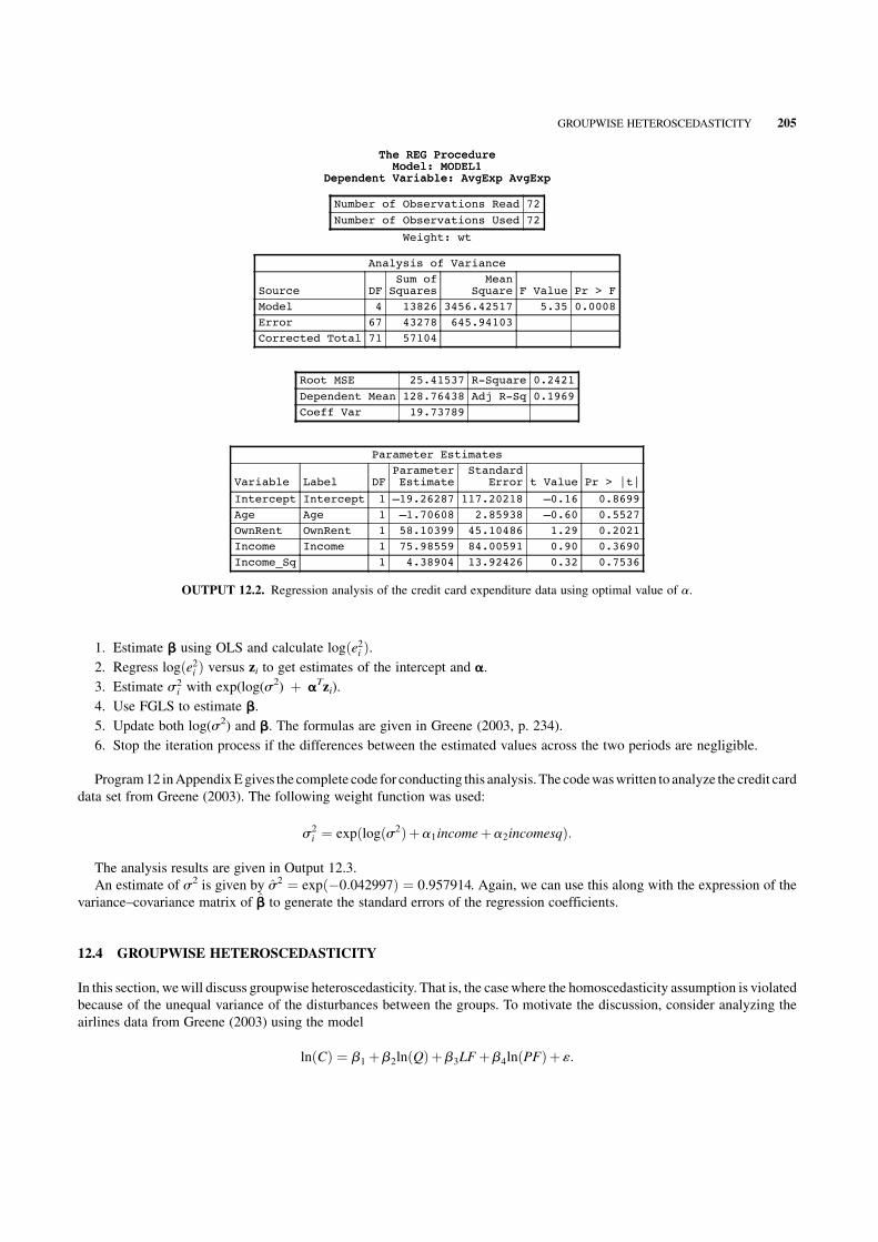
The REG ProcedureModel: MODEL1
Dependent Variable: AvgExp AvgExp
The REG ProcedureModel: MODEL1
Dependent Variable: AvgExp AvgExp
Number of Observations Read 72
Number of Observations Used 72
Weight: wt
Analysis of Variance
Source DFSum of
SquaresMean
Square F Value Pr > F
Model 4 13826 3456.42517 5.35 0.0008
Error 67 43278 645.94103
Corrected Total 71 57104
Root MSE 25.41537 R-Square 0.2421
Dependent Mean 128.76438 Adj R-Sq 0.1969
Coeff Var 19.73789
Parameter Estimates
Variable Label DFParameterEstimate
StandardError t Value Pr > |t|
Intercept Intercept 1 –19.26287 117.20218 –0.16 0.8699
Age Age 1 –1.70608 2.85938 –0.60 0.5527
OwnRent OwnRent 1 58.10399 45.10486 1.29 0.2021
Income Income 1 75.98559 84.00591 0.90 0.3690
Income_Sq 1 4.38904 13.92426 0.32 0.7536
OUTPUT 12.2. Regression analysis of the credit card expenditure data using optimal value of a.
1. Estimate b using OLS and calculate logðe2i Þ.
2. Regress logðe2i Þ versus zi to get estimates of the intercept and a.
3. Estimate s2i with exp(log(s2) þ aT
zi).
4. Use FGLS to estimate b.
5. Update both log(s2) and b. The formulas are given in Greene (2003, p. 234).
6. Stop the iteration process if the differences between the estimated values across the two periods are negligible.
Program12 inAppendixEgives the complete code for conducting this analysis. The codewaswritten to analyze the credit card
data set from Greene (2003). The following weight function was used:
s2i ¼ expðlogðs2Þþa1incomeþa2incomesqÞ:
The analysis results are given in Output 12.3.
An estimate of s2 is given by s2 ¼ expð�0:042997Þ ¼ 0:957914. Again, we can use this along with the expression of the
variance–covariance matrix of b to generate the standard errors of the regression coefficients.
12.4 GROUPWISE HETEROSCEDASTICITY
In this section, wewill discuss groupwise heteroscedasticity. That is, the casewhere the homoscedasticity assumption is violated
because of the unequal variance of the disturbances between the groups. To motivate the discussion, consider analyzing the
airlines data from Greene (2003) using the model
lnðCÞ ¼ b1 þb2lnðQÞþb3LFþb4lnðPFÞþ «:
GROUPWISE HETEROSCEDASTICITY 205

This data set was used extensively to illustrate basic panel datamodels inChapter 7. The least squares residualswas plotted for
each airline and appear in Figures 12.2 and 12.3.
Airlines 3, 4, and 6 exhibit more variability in the disturbances than the other airlines. We therefore suspect that the model
suffers from groupwise heteroscedasticity. A formal test to check this can be conducted by using the likelihood ratio test given by
(Greene, 2003, p. 236).
x20 ¼ nlnðs2Þ�
X
K
i¼1
nis2i :
ALPHA
The value of alpha is –0.042997
5.3553578
–0.563225
I
Convergence was obtained in 67 iterations.
The estimates of the coefficients are
STAT_TABLE
BHAT SE
INT –58.4173 60.7722
AGE –0.3763 0.5383
OWNRENT 33.3545 36.3445
INCOME 96.8136 31.1198
INCOME2 –3.7999 2.5688
OUTPUT 12.3. Maximum likelihood estimates using a multivariate value of a.
0 10 20 30 40 50 60 70 80 90
Obs
0.4
0.3
0.2
0.1
0.0
–0.1
–0.2
–0.3
Resid
uals
FIGURE 12.2. Time series plot of least squares residuals of individual airlines.
206 SPECIAL TOPICS

1 2 3 4 5 6
I
Resid
uals
0.4
0.3
0.2
0.1
0.0
–0.1
–0.2
–0.3
FIGURE 12.3. Side-by-side comparison of the least squares residuals of airlines.
This test statistic is a slightmodification of theBartlett test statistic to comparevariances (Snedecor andCochran, 1983).Here,
s2 is themean square error (MSE)when the data set is pooled across theK groups and s2i are the group-specificmean square errors.
Under the null hypothesis of homoscedasticity, the test statistic x20 has a chi-squared distribution with K� 1 degrees of freedom.
For the model given above, the value of x20 equals 107.4 and the null hypothesis of homoscedasticity is therefore rejected.
Another test that can be used to check for groupwise heteroscedasticity is the test by Bartlett (Snedecor and Cochran, 1983),
which is given by
x20 ¼
ðn�KÞlnðs2Þ�P
K
i¼1
ðni�1Þlnðs2i Þ
1þ 13ðK�1Þ
P
K
i¼1
1ni�1
� �
� 1n�K
� � :
The term in the numerator is theBartlett test statistic for comparingvariances and is very similar to the test statistic givenabove.
In general, a groupwise heteroscedasticitymodel is characterized by a common coefficients vector (or slopevector) across the
K groups but different within-group disturbance variances. That is, a model with the form (Greene, 2003, p. 235)
yi ¼ xTi bþ «i; i ¼ 1; . . . ; n;
Varð«ikjxiKÞ ¼ s2K ; i ¼ 1; . . . ; nK :
If thewithin-groupvarianceswithin eachgroupareknown, thenonecanuseGLSestimation to calculate anestimateof the least
squares parameter.However, inmost cases thiswill be unknown and estimationwill need to be done usingFGLS.That is, the least
squares estimates can be computed using
b ¼X
K
i¼1
1
s2i
XTi Xi
" #�1X
K
i¼1
1
s2i
XTi yi
" #
:
The within-group residuals vector, ei can be used to calculate s2i (i¼ 1, . . ., K). That is,
s2i ¼
eTi ei
ni; i ¼ 1; . . . ; K:
GROUPWISE HETEROSCEDASTICITY 207

The following statements can be used to analyze the airlines data set under thegroupwise heteroscedasticity assumption for the
model
lnðcostitÞ ¼ b1 þb2lnðoutputitÞþb3LoadFactorit þb4lnðFuelPriceitÞþa2Firm2 þa3Firm3 þa4Firm4 þa5Firm5 þa6Firm6 þ «it:
Weare assuming that a temporarySASdata set“airline”with the appropriate transformations anddummyvariables has already
been created.
Step 1: Conduct an OLS to calculate the residuals. The following statements can be used.
proc reg data=airline;
model LnC=LnQ LnPF LF delta2 delta3 delta4 delta5 delta6;
output out=resid r=resid;
run;
Step 2: Calculate the within-group estimate of the disturbance variance. The following statements can be used.
data get_resid;
set resid;
temp=resid*resid;
run;
proc univariate data=get_resid noprint;
var temp;
by i;
output out=out sum=sum n=n;
run;
data get_var;
set out;
var=sum/n;
run;
Step 3: Merge the original data set with the data set that contains the within-group variances, calculate the weights, and
estimate the parameters.
data final_analysis;
merge airline(in=a) get_var(in=b);
by i;
if a and b;
weight=1/var;
run;
proc reg data=final_analysis;
model LnC=LnQ LnPF LF delta2 delta3 delta4 delta5 delta6;
weight weight;
run;
The results of the analysis are given in Output 12.4. The first part of the output includes the traditional OLS model without
adjusting for the different within-group disturbance variances.
Another estimationmethod involves treating this model as a form of Harvey’s multiplicative heteroscedasticity model with ziequal to the set ofK� 1 dummy variables. Program 13 inAppendix E contains the IML code for analyzing the airlines data using
the Harvey’s multiplicative heteroscedasticity approach (Output 12.5). Here, zi contains K� 1 dummy variables.
208 SPECIAL TOPICS

The REG ProcedureModel: MODEL1
Dependent Variable: LnC
The REG ProcedureModel: MODEL1
Dependent Variable: LnC
Number of Observations Read 90
Number of Observations Used 90
Analysis of Variance
Source DFSum of
SquaresMean
Square F Value Pr > F
Model 8 113.74827 14.21853 3935.80 <0.0001
Error 81 0.29262 0.00361
Corrected Total 89 114.04089
Root MSE 0.06011 R-Square 0.9974
Dependent Mean 13.36561 Adj R-Sq 0.9972
Coeff Var 0.44970
Parameter Estimates
Variable Label DFParameterEstimate
StandardError t Value Pr > |t|
Intercept Intercept 1 9.70594 0.19312 50.26 <0.0001
LnQ 1 0.91928 0.02989 30.76 <0.0001
LnPF 1 0.41749 0.01520 27.47 <0.0001
LF LF 1 –1.07040 0.20169 –5.31 <0.0001
delta2 1 –0.04124 0.02518 –1.64 0.1054
delta3 1 –0.20892 0.04280 –4.88 <0.0001
delta4 1 0.18456 0.06075 3.04 0.0032
delta5 1 0.02405 0.07990 0.30 0.7641
delta6 1 0.08706 0.08420 1.03 0.3042
Number of Observations Read 90
Number of Observations Used 90
Weight: weight
Analysis of Variance
Source DFSum of
SquaresMean
Square F Value Pr > F
Model 8 46047 5755.82865 5526.84 <0.0001
Error 81 84.35595 1.04143
Corrected Total 89 46131
Root MSE 1.02051 R-Square 0.9982
Dependent Mean 13.47897 Adj R-Sq 0.9980
Coeff Var 7.57109
Parameter Estimates
Variable Label DFParameterEstimate
StandardError t Value Pr > |t|
Intercept Intercept 1 9.94232 0.16229 61.26 <0.0001
LnQ 1 0.92577 0.02678 34.57 <0.0001
LnPF 1 0.40561 0.01255 32.32 <0.0001
LF LF 1 –1.21631 0.18559 –6.55 <0.0001
delta2 1 –0.04603 0.02376 –1.94 0.0562
delta3 1 –0.20210 0.03615 –5.59 <0.0001
delta4 1 0.19055 0.05516 3.45 0.0009
delta5 1 0.03717 0.07044 0.53 0.5992
delta6 1 0.09459 0.07436 1.27 0.2070
OUTPUT 12.4. Groupwise heteroscedasticity estimators for the airlines data.

12.5 HAUSMAN–TAYLOR ESTIMATOR FOR THE RANDOM EFFECTS MODEL
Basic panel data models including both fixed and random effects models have been discussed in Chapter 7. A fundamental
assumption in random effects models is that the unobserved subject-specific heterogeneity is independent of the observed
explanatory variables. In reality, it is rare that this assumption holds. For example, both Baltagi (2005, p. 128) and Greene
(2003, p. 305) give an example of a study where the interest is to gauge the impact of years of schooling on earnings. It is well
known that a subject’s motivation and desire (both assumed unobserved) are highly correlated to academic success and,
therefore, to the subject’s number of years of formal schooling. The random effects model cannot be used here since the
independence assumption between the unobserved heterogeneity (motivation, desire) and observed explanatory variable
(number of years of schooling) is correlated. As discussed in Greene (2003), most often these models have explanatory
variables that are time invariant. That is, we may be interested in drivers such as gender, race, marital status, and so on with
respect to their impact on earning’s potential. However, fixed effects models cannot incorporate time-invariant explanatory
variables as they are “swept” from the model. Suppose that the researcher wants to include the time-invariant explanatory
variables in the model. In this case, the fixed effects model will not allow the estimation of the parameters of these time-
invariant explanatory variables.
Hausman and Taylor (1981) introduced estimation techniques for the random effects model where the unobserved subject-
specific heterogeneity is correlated with the observed explanatory variables and where there are time-invariant explanatory
variables in the model.
Hausman andTaylor’s general approach is to first partition the observed and unobserved explanatory variables into two sets. In
each set, one set of variables are exogenouswhile the other set of variables are endogenous.Using the notation fromGreene (2003,
p. 303), we can write the general form of the model as
yit ¼ xT1itb1 þ xT2itb2 þ zT1ia1 þ zT2ia2 þ eit þ ui; i ¼ 1; . . . ; n; t ¼ 1; . . . ; T :
I
Convergence was obtained in 12 iterations
The estimates of the coefficients are
ESTIMATES_GLS
BETA SE
INTERCEPT 10.0570 0.1343
LNQ 0.9283 0.0227
LF –1.2892 0.1638
LNPF 0.4000 0.0108
D2 –0.0487 0.0237
D3 –0.1996 0.0308
D4 0.1921 0.0499
D5 0.0419 0.0594
D6 0.0963 0.0631
The values of alpha are
ESTIMATES_ALPHA
ALPHA SE_ALPHA
ALPHA1 –7.0882 0.3651
ALPHA2 2.0073 0.5164
ALPHA3 0.7581 0.5164
ALPHA4 2.3855 0.5164
ALPHA5 0.5300 0.5164
ALPHA6 1.0530 0.5164
OUTPUT 12.5. Groupwise heteroscedasticity estimators for the airlines data using Harvey’s Multiplicative heteroscedasticity approach.
210 SPECIAL TOPICS

Here,
1. xT1it has k1 observed explanatory variables that are time dependent and exogenous with respect to ui.
2. z1 has l1 observed individual-specific variables that are time independent and exogenous with respect to ui.
3. xT2it has k2 observed explanatory variables that are time dependent and endogenous with respect to ui.
4. z2 has l2 observed individual-specific variables that are time independent and endogenous with respect to ui.
The assumptions about the random disturbances of this model are given in Greene (2003, p. 303). Hausman and Taylor
proposed an instrumental variables approach to estimate the parameters of the general model in the presence of the endogenous
variables. The Hausman and Taylor’s approach can be outlined as follows (Baltagi, 2005, p. 126; Greene, 2003, p. 304).
We can estimateb1 andb2 by using thewithin-group estimator. However, the time-invariant explanatory variables are “swept”
from the model and so we cannot estimate a1 and a2.
Note that in thewithin-groupmodel, the time-invariant disturbance term, ui, is swept from themodel as well and, therefore,
both sets of deviations ðx1it��x1i:Þ and ðx2it��x2i:Þ are independent of ui. Hausman and Taylor recommended that these k1 þ k2deviations be used as instruments to estimatea1 anda2. Next, since z1 is also exogenous, additional l1 instruments are available
for estimation. At this stage, the number of instruments is less than the number of parameters that need to be estimated. That is,
we have k1 þ k2 þ l1 instruments and k1 þ k2 þ l1 þ l2 parameters. As stated in Greene (2003), Hausman and Taylor show
that as long as k1� l2, the k1 group means �x1 can also be used as instruments. The complete set of instruments is, therefore,
given by
ðx1it��x1i:Þ; ðx2it��x2i:Þ; z1; �x1:
The following steps can then be taken to estimate a and b:
1. Estimateb1 andb2using x1 and x2 via thewithin-groupmodel. Estimates2«, the variance of «it, using the residuals from this
analysis.
2. Use the estimates of b1 and b2 from step 1 to get the within-group residuals. That is, calculate �ei: ¼ �yi:��xi:b where
b ¼ ðbT1 ; bT2 Þ. Instrumental variable regression is then used to regress the residual group means against z1 and z2 using as
instruments z1 and x1 to provide an estimate for a1 and a2.
3. Use the mean square errors from steps 1 and 2 to estimate s2u, the variance of ui, by using the formula s2
u ¼ s*2�s2«=T .
Next, define the weights that will be used in FGLS estimation as
u ¼
ffiffiffiffiffiffiffiffiffiffiffiffiffiffiffiffiffiffiffi
s2«
s2« þ Ts2
u
s
:
4. Calculate the weighted instrumental variable estimator using the weights from step 3. To proceed, first consider the row
vector wTit ¼ ðxT1it; x
T2it; z
T1i; z
T2iÞ. The transformed variables using the weights are given by the row vectors (Greene, 2003,
p. 305)
w*Tit ¼ wT
it�ð1�uÞ�wTi: ;
y*it ¼ yit�ð1�uÞ�yi::
The instrumental variables are given by the row vector
vTit ¼ b ðx1it��x1iÞT ðx2it��x2iÞ
TzT1i �xT1i Þc:
HAUSMAN–TAYLOR ESTIMATOR FOR THE RANDOM EFFECTS MODEL 211

Wecan then stack the rowvectors defined above to formnt� (2k1 þ k2 þ l1)matricesW*andV. LetY*be thenT� 1vector of
transformed responses. The instrumental variables estimator is, therefore, given by
ðbT; aTÞTIV ¼
�
ðW*TVÞðVTVÞ�1ðVTW*Þ
��1�
ðW*TVÞðVTVÞ�1ðW*TY*Þ
�
ðBaltagi; 2005; p: 126; Greene; 2003; p: 305Þ:
The standard errors of the coefficients can be calculated using the approaches discussed in the previous chapters.
Wewill now illustrate theHausman andTaylormethod on thePSID return to schooling data based on apanel of 595 individuals
observedover the period 1976–1982.The datawere analyzed byCornwell andRupert (1988) and then again byBaltagi (2005).As
described in Baltagi (2005, p. 128), the analysis involves regressing the log of wage on years of education (ED), weeks worked
(WKS), years of full-time work experience (EXP), occupation (OCC¼ 1, an indicator that the person is in a full-collar
occupation), location indicators SOUTH (1 if the person resides in the South), SMSA (1 if the person resides in a standard
metropolitan resident area), industry (IND¼ 1 if the person works in a manufacturing industry), marital status (MS¼ 1 if the
person is married), sex and race (FEM¼ 1 indicates that the person is a female, BLK¼ 1 indicates that the person is a black
individual), and union coverage (UNION¼ 1 if the person belongs to a union). We will compare the random effects and LSDV
model resultswith theHausman andTaylormodel.Taking an identical approach to analyzing the data as the author, the following
four groups of variables are first defined.
X1 ¼OCC, SOUTH, SMSA, IND.
X2 ¼EXP, EXP2, WKS, MS, UNION.
Z1 ¼FEM, BLK.
Z2 ¼ED.
The following statements can be used to fit a randomeffectsmodel to the data set. The analysis results are given inOutput 12.6.
proc panel data=wages;
id people year;
model lwage=EXP EXPSQ WKS OCC IND SOUTH SMSA MS FEM UNION
ED BLK/ranone;
run;
The variables EXP, EXPSQ, OCC, MS, FEM, UNION, ED, and BLK are all significant while the variables WKS, IND,
SOUTH, and SMSA are not significant. Since this is a semi-log model, we can interpret the coefficient for return to
schooling as follows: an additional year of schooling results in an 10.7% wage gain. Note that the test statistic for
Hausman’s test cannot be computed here because the fixed effects model eliminates the model FEM, BLK, and ED. If we
eliminate these variables from the model and rerun the random effects model using Proc Panel, we get a Hausman’s test
statistic value of 541.87 with 7 degrees of freedom that is highly significant. The correct degrees of freedom should be 9
since three explanatory variables were eliminated. Baltagi (2005, p. 128) gives the Hausman’s test statistic value that is
much larger than the one obtained by the Proc Panel procedure and has the correct degrees of freedom. We conducted the
Hausman’s test using Proc IML with the within-groups and random effects estimator and calculated the test statistics to be
higher than the one reported by the author. Nevertheless, the Hausman test statistic is rejected that justifies the use of an
instrumental variables approach.
As stated earlier, the random effects model does not take into account any possible correlation between the explanatory
variables and the unobserved individual subject-specific effects. Thewithin-group estimators can be calculated bymaking use of
the code provided inChapter 7—the code is also provided in the computations of theHausman–Taylor estimator. The results from
the analysis are given in Output 12.7.
As stated earlier, thewithin-groupmodel sweeps the individual effects from themodel resulting in a consistent estimator of the
parameters associated with the time-dependent explanatory variables. However, the approach does not allow us to estimate the
parameters of the time-invariant effects.
The following steps can be taken to obtain the coefficients estimates under theHausman–Taylor approach.Note that Proc IML
is used in conjunction with other SAS procedures. Also note that the results are slightly off from the results presented in Baltagi
(2005, Table 7.4, p. 129). The differences are, however, very small.
212 SPECIAL TOPICS

1. The groupmeans for the response variable and all explanatory variables are calculated using ProcUnivariate. The output is
stored in a temporary SAS data set called summary.
proc univariate data=wages noprint;
var occ south smsa ind exp expsq wks ms union fem blk
ed lwage;
by people;
output out=summary mean=m_occ m_south m_smsa m_ind
m_exp m_expsq m_wks m_ms m_union m_fem m_blk m_ed
m_lwage;
run;
The PANEL ProcedureFuller and Battese Variance Components (RanOne)
Dependent Variable: LWAGE LWAGE
Model Description
Estimation Method RanOne
Number of Cross Sections 595
Time Series Length 7
Fit Statistics
SSE 149.3005 DFE 4152
MSE 0.0360 Root MSE 0.1896
R-Square 0.4284
Variance Component Estimates
Variance Component for Cross Sections 0.100553
Variance Component for Error 0.023102
Hausman Test forRandom Effects
DF m Value Pr > m
0 . .
Parameter Estimates
Variable DF EstimateStandard
Error t Value Pr > |t| Label
Intercept 1 4.030811 0.1044 38.59 <0.0001 Intercept
EXP 1 0.087726 0.00281 31.27 <0.0001 EXP
expsq 1 –0.00076 0.000062 –12.31 <0.0001
WKS 1 0.000954 0.000740 1.29 0.1971 WKS
OCC 1 –0.04293 0.0162 –2.65 0.0081 OCC
IND 1 0.00381 0.0172 0.22 0.8242 IND
SOUTH 1 –0.00788 0.0281 –0.28 0.7795 SOUTH
SMSA 1 –0.02898 0.0202 –1.43 0.1517 SMSA
MS 1 –0.07067 0.0224 –3.16 0.0016 MS
FEM 1 –0.30791 0.0572 –5.38 <0.0001 FEM
UNION 1 0.058121 0.0169 3.45 0.0006 UNION
ED 1 0.10742 0.00642 16.73 <0.0001 ED
BLK 1 –0.21995 0.0660 –3.33 0.0009 BLK
OUTPUT 12.6. Random effects model for the wages data.
HAUSMAN–TAYLOR ESTIMATOR FOR THE RANDOM EFFECTS MODEL 213

The summary statistics are thenmergedwith the original data set to create a data setwhere the observations on each variable
are deviations from the group means. This is accomplished with the following statements.
data LSDV_Step;
merge wages(in=a) summary(in=b);
by people;
if a and b;
t_occ=occ-m_occ;
t_south=south-m_south;
t_smsa=smsa-m_smsa;
t_ind=ind-m_ind;
The REG ProcedureModel: MODEL1
Dependent Variable: t_lwage
The REG ProcedureModel: MODEL1
Dependent Variable: t_lwage
Number of Observations Read 4165
Number of Observations Used 4165
No intercept in model. R-Square is redefined.
Analysis of Variance
Source DFSum ofSquares
MeanSquare F Value Pr > F
Model 9 158.38388 17.59821 889.03 <0.0001
Error 4156 82.26732 0.01979
Uncorrected Total 4165 240.65119
Root MSE 0.14069 R-Square 0.6581
Dependent Mean 8.52992E-18 Adj R-Sq 0.6574
Coeff Var 1.649418E18
Model is not full rank. Least-squares solutions for the parameters are notunique. Some statistics will be misleading. A reported DF of 0 or B means thatthe estimate is biased.
The following parameters have been set to 0, since the variables are a linearcombination of other variables as shown.
t_fem = 0
t_blk = 0
t_ed = 0
Parameter Estimates
Variable DFParameterEstimate
StandardError t Value Pr > |t|
t_occ 1 –0.02148 0.01276 –1.68 0.0924
t_south 1 –0.00186 0.03175 –0.06 0.9533
t_smsa 1 –0.04247 0.01798 –2.36 0.0182
t_ind 1 0.01921 0.01430 1.34 0.1792
t_exp 1 0.11321 0.00229 49.49 <0.0001
t_expsq 1 –0.00041835 0.00005054 –8.28 <0.0001
t_wks 1 0.00083595 0.00055509 1.51 0.1321
t_ms 1 –0.02973 0.01757 –1.69 0.0908
t_union 1 0.03278 0.01381 2.37 0.0177
t_fem 0 0 . . .
t_blk 0 0 . . .
t_ed 0 0 . . .
OUTPUT 12.7. Within-group effects model for the wages data.
214 SPECIAL TOPICS

t_exp=exp-m_exp;
t_expsq=expsq-m_expsq;
t_wks=wks-m_wks;
t_ms=ms-m_ms;
t_union=union-m_union;
t_fem=fem-m_fem;
t_blk=blk-m_blk;
t_ed=ed-m_ed;
t_lwage=lwage-m_lwage;
run;<?}j?>
2. Proc IML is now used to calculate the within-group estimates and the within-group mean residuals. The group mean
residuals from this step are used as a dependent variable in an instrumental variable regression against z1 and z2 with
instruments x1 and z1.
proc iml;
use wages;
use LSDV_Step;
read all var{’t_occ’, ’t_south’, ’t_smsa’, ’t_ind’,
’t_exp’, ’t_expsq’, ’t_wks’, ’t_ms’, ’t_union’} into
X;
read all var{’t_lwage’} into Y;
beta=inv(X‘*X)*X‘*Y;
summary var{occ south smsa ind exp expsq wks ms union
lwage} class{people} stat{mean} opt{save};
Y_M=lwage;
X_M=occ||south||smsa||ind||
exp||expsq||wks||ms||union;
e=Y_M-X_M*beta;
create e_data from e;
append from e;
run;
3. A new data set is created with the within-group mean residuals and the explanatory variables for the purpose of doing the
instrumental variables regression. The following statements can be used.
data e_data;
set e_data;
people=_n_;
run;
data step2;
merge wages(in=a) e_data(in=b);
by people;
if a and b;
rename col1=e_mean;
run;
The instrumental variable regression is done by using Proc Model. The following statements can be used. The analysis
results are given in Output 12.8.
proc model data=step2;
endo ed;
instruments fem blk occ south smsa ind;
e_mean=beta2*fem+beta3*blk+beta4*ed;
HAUSMAN–TAYLOR ESTIMATOR FOR THE RANDOM EFFECTS MODEL 215

The MODEL ProcedureThe MODEL Procedure
Model Summary
Model Variables 4
Endogenous 3
Parameters 3
Equations 1
Number of Statements 1
Model Variables FEM BLK ED e_mean
Parameters beta2 beta3 beta4
Equations e_mean
The Equation to Estimate is
e_mean = F(beta2(FEM), beta3(BLK), beta4(ED))
Instruments 1 FEM BLK OCC SOUTH SMSA IND
NOTE: At 2SLS Iteration 1 CONVERGE=0.001 Criteria Met.
The MODEL Procedure2SLS Estimation Summary
Data SetOptions
DATA= STEP2
Minimization Summary
Parameters Estimated 3
Method Gauss
Iterations 1
Final ConvergenceCriteria
R 0
PPC 0
RPC(beta4) 3549.228
Object 0.992621
Trace(S) 1.24545
Objective Value 0.160006
ObservationsProcessed
Read 4165
Solved 4165
OUTPUT 12.8. Proc model output (preliminary step) to the Hausman and Taylor estimates for the wages data.
216 SPECIAL TOPICS

fit e_mean/2sls;
run;
4. The final step is to calculate theweighted instrumental variables estimator. From thewithin-groups analysis, an estimate of
s2eis 0.0231 and from the instrumental regression analysis, an estimate of s*2 is 1.2454. These values can be used to
calculate an estimate of s2u. That is,
s2u ¼ s*2�s2
«=T
¼1:2454�0:0231=7
¼1:2421:
An estimate of the weight, u, can now be derived as follows:
u ¼
ffiffiffiffiffiffiffiffiffiffiffiffiffiffiffiffiffiffiffi
s2«
s2« þ Ts2
u
v
u
u
t
¼
ffiffiffiffiffiffiffiffiffiffiffiffiffiffiffiffiffiffiffiffiffiffiffiffiffiffiffiffiffiffiffiffiffiffiffiffiffiffiffiffiffi
0:0231
0:0231þ 7� 1:2421
s
¼ 0:051476:
The calculation is carried out in the following data step statements in SAS. The variables are also transformed using this
weight in the following statements.
data Final_Step;
merge wages(in=a) summary(in=b);
by people;
if a and b;
sigmae=0.0231;
The MODEL Procedure
Nonlinear 2SLS Summary of Residual Errors
EquationDF
ModelDF
Error SSE MSE Root MSE R-SquareAdj
R-Sq
e_mean 3 4162 5183.6 1.2454 1.1160 –0.1664 –0.1670
Nonlinear 2SLS Parameter Estimates
Parameter EstimateApproxStd Err t Value
ApproxPr > |t|
beta2 –0.12485 0.0560 –2.23 0.0258
beta3 0.056205 0.0679 0.83 0.4080
beta4 0.358572 0.00143 250.24 <0.0001
Number ofObservations Statistics for System
Used 4165 Objective 0.1600
Missing 0 Objective*N 666.4242
OUTPUT 12.8. (Continued )
HAUSMAN–TAYLOR ESTIMATOR FOR THE RANDOM EFFECTS MODEL 217

sigmau=1.2421;
Theta=sqrt(sigmae/(sigmae+7*sigmau));
t_occ=occ-(1-theta)*m_occ;
t_south=south-(1-theta)*m_south;
t_smsa=smsa-(1-theta)*m_smsa;
t_ind=ind-(1-theta)*m_ind;
t_exp=exp-(1-theta)*m_exp;
t_expsq=expsq-(1-theta)*m_expsq;
t_wks=wks-(1-theta)*m_wks;
t_ms=ms-(1-theta)*m_ms;
t_union=union-(1-theta)*m_union;
t_fem=fem-(1-theta)*m_fem;
t_blk=blk-(1-theta)*m_blk;
t_ed=ed-(1-theta)*m_ed;
t_lwage=lwage-(1-theta)*m_lwage;
s_occ=occ-m_occ;
s_south=south-m_south;
s_smsa=smsa-m_smsa;
s_ind=ind-m_ind;
s_exp=exp-m_exp;
s_expsq=expsq-m_expsq;
s_wks=wks-m_wks;
s_ms=ms-m_ms;
s_union=union-m_union;
s_fem=fem-m_fem;
s_blk=blk-m_blk;
s_ed=ed-m_ed;
run;
Proc IML is then used to calculate the Hausman–Taylor’s estimates for the earnings equation. The analysis results are given in
Output 12.9. The model indicates that an additional year of schooling results in a 13.73% wage gain. This is significantly
different from the estimate obtained from the random effects model.
proc iml;
* Read the data into matrices.;
use final_step;read all
var{’t_occ’,’t_south’,’t_smsa’,’t_ind’,’t_exp’,
’t_exsq’,’t_wks’,’t_ms’,’t_union’,
’t_fem’,’t_blk’,’t_ed’} into W;
read all var{t_lwage} into Y;
W=J(4165,1,0.051408)||W;
read all
var{’s_occ’,’s_south’,’s_smsa’,’s_ind’,’s_exp’,
’s_expsq’,’s_wks’,’s_ms’,’s_union’,
’fem’,’blk’,’m_occ’,’m_south’,’m_smsa’,’m_ind’} into
V;
* Calculate the Hausman and Taylor estimates and standard
errors.;
HT=inv((W‘*V)*inv(V‘*V)*(V‘*W))*((W‘*V)*inv(V‘*V)*(V‘
*y));
MSE=(y-W*HT)‘*(y-W*HT)/(4165);
SE=SQRT(vecdiag(MSE*inv((W‘*V)*inv(V‘*V)*(V‘*W))));
run;
218 SPECIAL TOPICS

The Hausman & Taylor Estimates are
TABLE1
BHAT SE
INTERCEPT 2.2098 0.2712
OCC –0.0209 0.0135
SOUTH 0.0052 0.0319
SMSA –0.0419 0.0189
IND 0.0152 0.0150
EXP 0.1132 0.0024
EXP_SQ –0.0004 0.0001
WKS 0.0008 0.0006
MS –0.0298 0.0186
UNION 0.0328 0.0146
FEM –0.1291 0.1481
BLK –0.2852 0.1798
ED 0.1373 0.0282
OUTPUT 12.9. Hausman and Taylor estimates of the wages equation.
12.6 ROBUST ESTIMATION OF COVARIANCE MATRICES IN PANEL DATA
The panel datamodels discussed in Chapter 7were based on the assumption of homoscedastic disturbances. This section extends
the discussion to heteroscedasticity in panel data models. We will focus our attention on the robust estimation of the covariance
matrix for fixed effects models and will use the Proc Panel procedure to calculate various robust estimates of the covariance
matrix. We illustrate the various techniques by revisiting the cost of US airlines data set from Greene (2003).
The HCCME option in Proc Model can be adjusted to generate robust estimates of the variance–covariance matrix. The
various options are given below (The Panel Procedure, p. 58, SAS Institute, Inc.). Also see the discussion on heteroscedasticity
in Chapter 5.
If we do not specify the HCCME option, then the analysis will default the OLS estimate of the covariance matrix. The OLS
output for the airlines data has been given in Chapter 7.
HCCME¼ 0: This yields the White’s estimator
1
nT
X
nT
i¼1
«2i xixTi :
HCCME¼ 1: This yields the first version of the Davidson and MacKinnon (1993) estimator where the end result of the
White’s estimator is scaled up by a factor of nT/(nT�K):
1
nT
X
nT
i¼0
nT
nT�K«2i xix
Ti
� �
:
HCCME¼ 2: This yields the secondversion of theDavidson andMacKinnon (1993) estimatorwhere theWhite’s estimator is
adjusted by the diagonals of the hat matrix:
hi ¼ XiðXTXÞ�1
XTi :
The estimator is given by
1
nT
X
nT
i¼0
«2i
1�hixix
Ti :
ROBUST ESTIMATION OF COVARIANCE MATRICES IN PANEL DATA 219

HCCME¼ 3: This yields an estimator that is similar to the second version of the Davidson andMacKinnon’s estimator. The
adjustment is now based on ð1�hiÞ2instead of ð1�hiÞ.
1
nT
X
nT
i¼0
«2i
ð1�hiÞ2xix
Ti :
HCCME¼ 4: This yields the Arellano (1987) version of the White’s estimator for panel data. The general idea involves
calculating theWhite’s estimator for each cross section in the panel (i¼ 1, . . ., n) and then taking the average of the n estimates of
the covariance matrices. See the Proc Panel Procedure (p. 58) for more details on this estimator.
Section 5.5 included a SAS program to print the various robust covariance matrices under heteroscedasticity. The code can
easily be adjusted to generate the robust covariance matrices in the panel setting.
The results of the analysis are given in Output 12.10. The diagonal elements in each covariance matrix give the variance
estimates for the parameters. Notice the similarity betweenWhite’s estimator and theDavidson andMcKinnon’s estimators. The
OLS estimators and the Arellano’s version of the White’s estimator are different from these.
12.7 DYNAMIC PANEL DATA MODELS
We now turn our attention to dynamic panel data models. That is, models that are characterized by lagged variables on the
right-hand side of the model. The general form of these models is given by Baltagi (2005, pp. 134–142) and Verbeek (2004,
pp. 360–366)
yi;t ¼ ryi;t�1 þ xTi;tbþai þ ei;t i ¼ 1; . . . ; n; t ¼ 1; . . . ; T
where yi,t is a 1� 1 scalar dependent variable, xi,t is a k� 1 vector of explanatory variables, and r and b are 1� 1 and k� 1
parameters that need to be estimated. The term ai is the unobserved subject-specific heterogeneity and «i,t is the disturbance.
The subscripts i and t index the subjects and the time period, respectively. As shown by Verbeek (2004, p. 361), the use of
lagged dependent variables on the right-hand side of the model introduces estimation problems, more specifically, with the
fixed effect model estimator becoming biased regardless of whether ai is treated as fixed or random. This section focuses on
methods based on generalizedmethods of moments estimation (GMM) that can be used to estimate the parameters in dynamic
panel data models.
Obs _TYPE_ _NAME_ LnQ LnPF LF
1 OLS LnQ 0.000893416 –0.000317817 –0.00188
2 OLS LnPF –0.000317817 0.000231013 –0.00077
3 OLS LF –0.001884262 –0.000768569 0.04068
4 HCCME0 LnQ 0.000365016 –0.000125245 –0.00031
5 HCCME0 LnPF –0.000125245 0.000183132 –0.00169
6 HCCME0 LF –0.000306158 –0.001690757 0.04692
7 HCCME1 LnQ 0.000405574 –0.000139161 –0.00034
8 HCCME1 LnPF –0.000139161 0.000203480 –0.00188
9 HCCME1 LF –0.000340176 –0.001878619 0.05214
10 HCCME2 LnQ 0.000397411 –0.000134190 –0.00034
11 HCCME2 LnPF –0.000134190 0.000192432 –0.00178
12 HCCME2 LF –0.000337505–0.001783683 0.04989
13 HCCME3 LnQ 0.000435062 –0.000144422 –0.00038
14 HCCME3 LnPF –0.000144422 0.000202471 –0.00188
15 HCCME3 LF –0.000378817 –0.001881047 0.05310
16 HCCME4 LnQ 0.000870151 0.000062860 –0.00794
17 HCCME4 LnPF 0.000062860 0.000301454 –0.00164
18 HCCME4 LF –0.007938291 –0.001642741 0.14797
OUTPUT 12.10. HCCME estimators for the airlines data set.
220 SPECIAL TOPICS

12.7.1 Dynamic Panel Data Estimation
The estimation technique is based on the class of GMM estimators introduced by Arnello and Bond (1991). They proposed an
estimation method based on instrumental variables estimation. As will be seen, the authors took advantage of the independence
between the laggedvaluesof thedependent variable and thedisturbances.Theirgeneralmethodand formulas canbe found inmost
intermediate–advanced texts on econometrics. I have found Baltagi (2005), Greene (2003), and Verbeek (2004) very useful in
understanding themechanics of theArellano andBond estimator. TheProc Panel documentation fromSAS Institute, Inc. is also a
good reference as it summarizes the key steps and formulas in the estimation process.
A discussion of GMM estimators is beyond the scope of this book (see the above mentioned texts for details). In general,
assuming the classical linear model y¼Xb þ e where X is suspected of being endogenous and where there is a matrix of
instruments Z, the GMM estimator takes the form
b ¼ ðXTZWZTWÞ�1XTZWZTy
whereW is called theweights matrix and is chosen tominimize the asymptotic covariance of b. GMMestimation is usually done
in two steps using an initial weight matrix (not optimal) in step 1. The optimal weight matrix is then formed using the residuals
from step 1 to calculate the second step GMM estimator.
The estimation steps are best understood by considering a basic dynamic panel data model without exogenous variables.
Consider the following simple autoregressive random effects panel model (Baltagi, 2005, p. 136; Verbeek, 2004, p. 361):
yi;t ¼ ryi;t�1 þai þ «i;t; i ¼ 1; . . . n; t ¼ 1; . . . ; T ;
where ai and «i,t are independently and identically distributed disturbances with variances s2a and s
2«, respectively. Furthermore,
assume that ai and «i,t are independent of each other.
An initial approach is to take the first differences since this “sweeps” the unobserved individual effects ai from the model
resulting in
yi;t�yi;t�1 ¼ rb yi;t�1�yi;t�2cþ b«i;t�«i;t�1c:
However, theOLS estimator of rwill still be biased and inconsistent sinceCov(yi,t�1,«i,t�1) 6¼ 0. To see how instrumental variable
estimation can be used to estimate r, consider the differencemodel at t¼ 1, 2, . . .. Obviously, this model is valid for the first time
when t¼ 3. The difference model is given by
yi;3�yi;t�2 ¼ rb yi;2�yi;1cþ b«i;3�«i;2c:
Here, yi,1 is avalid instrument since it is highly correlated to y2,i� y1,ibut is uncorrelated to«i,3� «i,2. Further,we can see that at
t¼ 4, the differenced model is
yi;4�yi;3 ¼ rb yi;3�yi;2cþ b«i;4�«i;3c
and now both yi,1 and yi,2 are valid instruments as both are uncorrelated with «i,4� «i,3. In this fashion, we see that the set of
instrumental variables for a given time period t is yi,1, . . ., yi,t�2, i¼ 1, . . ., n (Baltagi, 2005, p. 137).
If Zi denotes the p� (T� 2) matrix of instruments for the i th subject, then it is easy to see that
ZTi ¼
yi;1 0 0 . . . . . . 0
0 yi;1 0 . . . . . . 0
0 yi;2 0 . . . . . . 0
0 0 . . . . . . . . . 0
..
. ... . .
. . ..
0 yi;1
..
. ... . .
. . ..
0 yi;2
..
. ... . .
. . ..
0 ...
0 0 . . . . . . . . . yi;T�2
2
6
6
6
6
6
6
6
6
6
6
6
6
6
6
6
6
4
3
7
7
7
7
7
7
7
7
7
7
7
7
7
7
7
7
5
:
DYNAMIC PANEL DATA MODELS 221

The number of rows in Zi equals p ¼PT�2
t¼1 t. If we combine the instrument variables matrix for all cross sections, we have
ZT ¼ ZT1 ZT
2 . . . ZTn�
�
.
The weight matrix for the first-step estimator is given by ZTHZ with Hi¼ diag[H1, . . ., Hn] where
Hi ¼
2 �1 0 . . . 0
�1 2 �1 . .. ..
.
0 . .. . .
. . ..
0
..
. . ..
�1 2 �1
0 . . . 0 �1 2
2
6
6
6
6
6
6
6
6
4
3
7
7
7
7
7
7
7
7
5
:
The (T� 2)� (T� 2) matrix Hi can be constructed as follows:
1. For the ith cross section, denote the vector of differenced residuals, Dei as
Dei ¼ ð«i;3�«i;2; . . . ; «i;T�«i;T�1Þ:
2. The diagonal elements of the matrix are given by EðD«2i;tÞ ¼ 2s2« while the off-diagonal elements are given by
EðD«i;tD«i;t�1Þ ¼ �s2«, and E(D«i,tD«i,t�s)¼ 0 for S� 2.
Notice that s2« cancels out in the subsequent steps and is therefore not included in Hi. If we denote the T� 2 difference
terms for all n cross sections as Dy, Dy�1, and De, we can write the difference model as Dy¼ rDy�1 þ De, then Arellano
and Bond’s first-step estimator is given by
rGMM1 ¼ DyT�1ZðZTHZÞ�1
ZTDy�1
h i�1
� DyT�1ZðZTHZÞ�1
ZTDy
h i
:
The residuals from this step are given by
De1i ¼ Dyi�rGMM1Dyi;�1 for i ¼ 1; . . . ; n
and are used to construct the weight matrix for the second-step estimator. That is, if we let V ¼ DeDeT , then the weight
matrix for the second-step estimator is given by ZTVZ. Arellano and Bond’s second-step estimator is given by
rGMM 2 ¼ DyT�1ZðZTVZÞ�1
ZTDy�1
h i�1
� DyT�1ZðZTVZÞ�1
ZTDy
h i
:
The following computational formulas for the various terms in theGMMcalculations are usefulwhen programming the
estimation method in Proc IML.
ZTHZ ¼X
n
i¼1
ZTi HiZi;
DyT�1Z ¼X
n
i¼1
DyTi;�1Zi;
and
DyTZ ¼X
n
i¼1
DyTi Zi:
Wewill illustrate the GMMmethod for this simple model on the cigar.txt panel data used by Baltagi and Levin (1992).
Consider the model (see Baltagi, 2005, pp. 156–158)
lnCi;t ¼ rlnCi;t�1 þai þ «i;t i ¼ 1; . . . ; 46; t ¼ 1; . . . ; 30:
As discussed by the author, the data set consists of real per capita sales of cigarettes (Ci,t) in 46 states (n¼ 46) between
1963 and 1992 (T¼ 30). Themodel contains the lag of this endogenous variable and therefore an OLS estimate of rwill be
222 SPECIAL TOPICS

inconsistent. The authors fit a more complex dynamic panel model, whichwill be discussed subsequently. For themoment,
we are interested in estimating the basic model given above.
Program 14 in Appendix E contains the complete Proc IML code for estimating both a one- and a two-step GMM estimate
for r. We leave it as an exercise to verify that the coefficients from the two GMM procedures give values of 1.031457 and
1.031563, respectively. It is very easy to extract the standard errors of the first- and second-step estimators andwe leave the
details as an exercise for the reader.
12.7.2 Dynamic Panel Data Models with Explanatory Variables
We now turn our attention to dynamic panel data models with explanatory variables. The general form of the model was given in
the earlier section. The Arellano and Bond (1991) GMM estimator used in the simple model with no explanatory variables can
easily be modified to the case involving explanatory variables.
As before, note that the presence of lagged variables on the right-hand side leads to biased and inconsistent estimators
of the parameters. We proceed by taking the first difference of the model and observing the following relationship:
yi;t�yi;t�1 ¼ r yi;t�1�yi;t�2 þ xTi;t�xTi;t�1
h i
bþi h
«i;t�«i;t�1
h i
:
OLS cannot be used here to estimate the parameters becauseCov(yi,t�1,«i,t�1) 6¼ 0. Also note that the difference relationship is
observed for the first time when t¼ 3 and is given by
yi;3�yi;2 ¼ r½yi;2�yi;1� þ ½xTi;3�xTi;2�bþ ½«i;3�«i;2�:
Earlier, we saw that yi,1 can be used as an instrument for yi,2� yi,1 because it is highly correlated with it and is uncorrelated to
«i,3� «i,2. Assuming that the explanatory variables are strictly exogenous, we can use all of them as additional instruments for
estimating the parameters. That is, the instrumental variables matrix Zi is given by
Zi ¼
yi;1; xTi;1; . . . ; x
Ti;T
h i
0 . . . 0
0 yi;1; yi;2; xTi;1; . . . ; x
Ti;T
h i
. . . 0
..
. ... . .
. ...
0 . . . yi;1; . . . ; yi;T�2; xTi;1; . . . ; x
Ti;T
h i
2
6
6
6
6
6
6
6
4
3
7
7
7
7
7
7
7
5
:
Under the assumption that the explanatory variables are predetermined, we know that E(xi,s«i,t)¼ 0 for s< t and 0 otherwise.
Therefore, we can use xi,t as instruments up to the same time period as the error term. That is, at time s, only xTi;1; . . . ; xTi;s�1 are
valid instruments in the first differenced equation.Thematrix of instrumentsZi in the predetermined case is givenbyArellano and
Bond (1991) and Baltagi (2005, p. 140):
Zi ¼
yi;1; xTi;1; x
Ti;2
h i
0 . . . 0
0 yi;1; yi;2; xTi;1; x
Ti;2; x
Ti;3
h i
. . . 0
..
. ... . .
. ...
0 . . . yi;1; . . . ; yi;T�2; xTi;1; . . . ; x
Ti;T�1
h i
2
6
6
6
6
6
6
6
4
3
7
7
7
7
7
7
7
5
:
The following formulation of the GMM estimator assumes that the explanatory variables are predetermined. The
Arellano–Bond estimation method in the more general case involves first constructing Zi as defined above along with Hi
(see Section 12.7.1). The weight matrix for the first-step GMM estimator is given by ZTHZ where Z andH are as defined in
DYNAMIC PANEL DATA MODELS 223

Section 12.7.1. Next, for the i th deviation, stack all the deviations and construct Xi and Yi as follows:
Xi ¼
Dyi;2 DxTi;3
Dyi;3 DxTi;4
..
. ...
Dyi;T�1 DxTi;T
2
6
6
6
6
6
4
3
7
7
7
7
7
5
andYi ¼
Dyi;3
Dyi;4
..
.
Dyi;T
2
6
6
6
6
4
3
7
7
7
7
5
:
Stacking Xi, Yi for all cross sections, we have
Z ¼
Z1
Z2
..
.
Zn
2
6
6
6
6
4
3
7
7
7
7
5
; X ¼
X1
X2
..
.
Xn
2
6
6
6
6
4
3
7
7
7
7
5
; andY ¼
Y1
Y2
..
.
Yn
2
6
6
6
6
4
3
7
7
7
7
5
:
Therefore, the Arellano–Bond first-step estimator is given by
dGMM1 ¼ ½XTZðZTHZÞ�1ZTX��1½XTZðZTHZÞ�1
ZTY�:
The residuals from the first-step GMM analysis is given by
De1i ¼ Yi�XidGMM1
and is used to create the optimal weight matrix ZTVZ where V ¼ DeDeT and is used in place of ZTHZ to generate the two-step
Arellano–Bond GMM estimator
dGMM 2 ¼ ½XTZðZTVZÞ�1ZTX��1½XTZðZTVZÞ�1
ZTY�:
Weillustrate theArellano andBondGMMestimationmethod in thegeneral case on the cigar.txt panel data used byBaltagi and
Levin (1992). Consider the full model (Baltagi, 2005, p. 156) given by
lnCi;t ¼ rlnCi;t�1 þb1lnPi;t þb2lnYi;t þb3lnPni;t þai þ «i;t
with i¼ 1, . . ., 46 and t¼ 1, . . ., 30.Here, i and t index the states and the time periods, respectively.As described by the author,Ci,t
is the average number of packs of cigarette sales per person over the age of 14,Pi,t is the average retail price of a pack of cigarettes,
Yi,t is the disposable income, and Pni,t is the minimum price of cigarettes in the adjoining states.
Program 15 in Appendix E contains the complete Proc IML code for estimating the cigarette panel data model using the
Arellano–Bond method. The reader is asked to verify that the first-step estimates are r¼ 0.799 b1¼�0.259, b2¼ 0.138,
and b3¼ 0.065 and that the second-step estimates are r¼ 0.79, b1¼�0.26, b2¼ 0.139, and b3¼ 0.033. It is very easy to
extract the standard errors of the first- and second-step GMM estimators. We leave the details as an exercise for the reader.
12.8 HETEROGENEITYAND AUTOCORRELATION IN PANEL DATA MODELS
This section dealswith analyticalmethodswhere the subjectsmaybe correlatedwith each other andwhere heterogeneity is due to
significant differences between thewithin subject (cross section) variances.Wewill also look at the case of autocorrelationwhere
the correlation is across the time periods.As discussed inGreene (2003, p. 320), a formulation of themodel,where the conditional
mean is assumed to be the same across the cross sections, can be written as
yit ¼ xTitbþ «it or yi ¼ Xibþ «i;
224 SPECIAL TOPICS

where i indexes the subjects and t indexes time and we assume that each Xi is exogenous. Stacking the equations across the n
subjects yields Y¼Xb þ e where Y is nT� 1, X is nT� k, b is k� 1, and e is nT� 1.
If we assume that the subjects are correlatedwith each other and that there is correlation across the time periods aswell, then
for the (i, j)th subjects, EðeieTj jXÞ ¼ Vij. The cross-sectional variance across groups can therefore be written as
EðeeT jXÞ ¼ V ¼
V11 V12 . . . V1n
V21 V22 . . . V2n
..
. ... . .
. ...
Vn1 Vn2 . . . Vnn
2
6
6
6
6
4
3
7
7
7
7
5
:
As shown in Greene (2003), each Vij is a T� T matrix that incorporates both the cross-sectional and the cross-period
correlations. For the case where there is no correlation across the time periods, the above can be rewritten as
EðeeT jXÞ ¼ V ¼
s11I s12I . . . s1nI
s21I s22I . . . s2nI
..
. ... . .
. ...
sn1I sn2I . . . snnI
2
6
6
6
6
4
3
7
7
7
7
5
where the sij’s capture the cross-sectional correlations.
12.8.1 GLS Estimation
As stated in Greene (2003, p. 321), the full generalized linear regression model using V consists of nT(nT þ 1)/2 unknown
parameters. Estimation is not possiblewithnTobservations unless restrictions are placedon theseparameters.A simple restriction
is to assume that there is no correlation across timeperiods that givesus the simplifiedversionofVgivenabove. Ifwe letS¼bsijc,then we can rewrite the variance–covariance matrix as V¼S� I. Using the methods from Chapter 5, we can write the GLS
estimator of b as
bGLS ¼ ðXTV�1XÞ�1
XTV�1y:
As shown by Greene (2003), if we let V�1¼S�1� I¼bsijc� I, then the GLS estimator is
bGLS ¼X
n
i¼1
X
n
j¼1
sijXTi Xj
" #�1X
n
i¼1
X
n
j¼1
sijXTi yj
" #
with asymptotic variance given by
Asy:VarðbGLSÞ ¼ ðXTV�1XÞ�1:
12.8.2 Feasible GLS Estimation
Inpractice,V is unknownandhas tobeestimatedusingFGLSmethods estimators.Theanalysis is done in twosteps. In step1,OLS
is used on the stackedmodel to obtain the residuals. Estimates ofsij are given by sij ¼ eTi ej=T (Greene, 2003, p. 322).With sij in
hand, the FGLS estimators can easily be calculated.
The groupwise heteroscedasticity estimator that was discussed in Chapter 5 is a special case of the FGLS estimator here
with the off-diagonal elements of S equal to 0. Here, we are assuming that there is no cross-sectional correlation and no
correlation across the time periods. However, the cross-sectional variances are significantly different from each other.
HETEROGENEITYAND AUTOCORRELATION IN PANEL DATA MODELS 225

Using the methods from Chapter 5, the groupwise heteroscedasticity estimator is given by Greene (2003, p. 323):
bGLS ¼X
n
i¼1
1
s2i
XTi Xi
" #�1X
n
i¼1
1
s2i
XTi yi
" #
:
Estimatingsi as before and using it in the above equation gives the FGLS estimator.Wewill now illustrate the steps involved in
the Grunfeld data set. The Proc IML code is given below.
Proc IML;
*Read the data into appropriate matrices;
Use SUR;
Read all var{’F’ ’C’} into X;
Read all var{’I’} into Y;
*Store the dimensions of X;
r=nrow(X);c=ncol(X);
*Append a column of 1’s to X;
X=J(r,1,1)||X;
*Conduct OLS to get pooled OLS model and calculate the residuals;
*This is step 1 of the procedure;
BHAT1=inv(X‘*X)*X‘*Y;
E1=Y-X*BHAT1;
*Conduct the groupwise heteroscedastic analysis.;
*This is step 2 of the procedure;
compt=1;
M=5;
T=20;
Temp0=0;Temp1=shape(0,3,3);Temp2=shape(0,3,1);
do i=1 to M;
Temp0=E1[compt:compt+t-1,1]‘*E1[compt:compt+t-1,1]/T;
Temp1=Temp1+1/Temp0*X[compt:compt+t-
1,1:3]‘*X[compt:compt+t-1,1:3];
compt=compt+t;
end;
compt=1;
do i=1 to M;
Temp0=E1[compt:compt+t-1,1]‘*E1[compt:compt+t-1,1]/T;
Temp2=Temp2+1/Temp0*X[compt:compt+t-
1,1:3]‘*Y[compt:compt+t-1,1];
compt=compt+t;
end;
BHAT_GRP=inv(Temp1)*Temp2;
Print ’The Groupwise Heteroscedastic Parameter Estimates
Are’;
Print BHAT_GRP;
*Now, calculate the asymptotic covariance matrix;
Grp_Sig=Shape(0,5,1);
compt=1;
do i=1 to M;
Grp_Sig[i,1]=E1[compt:compt+t-1,1]‘*E1[compt:compt+t-
1,1]/T;
compt=compt+T;
end;
Cap_Sigma=diag(Grp_Sig);
226 SPECIAL TOPICS

ID=I(T);
Omega=Cap_Sigma@ID;
Asy_Var=inv(X‘*inv(Omega)*X);
Print ’The Asymptotic Covariance Matrix Is’;
Print Asy_Var;
SE=sqrt(vecdiag(Asy_Var));
Print ’The Asymptotic Standard Errors Are’;
Print SE;
*Now, we get the residuals from the Groupwise Heterogeneity Regression;
E2=Y-X*BHAT_GRP;
*The final step is to calculate the SUR Pooled estimator.;
*The standard errors are also calculated.;
temp1=e2[1:20,1]||e2[21:40,1]||e2[41:60,1]||e2[61:80,1]||e2
[81:100,1];
countt=1;
temp1=E2[countt:t,1];
do i=2 to M;
countt=countt+t;
c=E2[countt:countt+t-1,1];
temp1=temp1||c;
end;
temp2=1/t*temp1‘*temp1;
I=I(20);
Temp3=temp2@I;
BETA_FGLS=inv(X‘*inv(Temp3)*X)*X‘*inv(Temp3)*Y;
Print ’The FGLS Parameter Estimates Are’;
Print BETA_FGLS;
Asy_Var=inv(X‘*inv(Temp3)*X);
Print ’The Asymptotic Covariance Matrix Is’;
Print Asy_Var;
SE=sqrt(vecdiag(Asy_Var));
Print ’The Asymptotic Standard Errors Are’;
Print SE;
*Now, calculate the cross-equation covariance for the SUR pooled model;
E3=Y-X*BETA_FGLS;
countt=1;
temp1=E3[countt:t,1];
do i=2 to M;
countt=countt+t;
c=E3[countt:countt+t-1,1];
temp1=temp1||c;
end;
temp2=1/t*temp1‘*temp1;
Print ’The Cross-Equation Covariance Matrix is’;
Print temp2;
run;
The analysis results are given in Output 12.11. Notice that the parameters have the same signs and similar magnitudes as the
ones obtained by OLS.
12.9 AUTOCORRELATION IN PANEL DATA
Wewill nowdealwith estimationmethodswhen thedisturbances are correlatedwithin cross sections andacross cross sections. The
simplest case is toassumethat there is nocorrelationbetween thedisturbances across cross sections.That is,Corr(«it,«js)¼ 0 if i 6¼ j.
AUTOCORRELATION IN PANEL DATA 227

Next, define the AR(1) process «it¼ ri«i,t�1 þ uit for the general linear model where (see Chapter 6 and Greene, 2003,
p. 325)
Varð«itÞ ¼ s2i ¼
s2ui
1�r2i:
We can use the methods of Chapter 6 to estimate b. That is,
The Groupwise Heteroscedastic Estimators are
TABLE1
BHAT SE
INTERCEPT –36.2537 6.1244
F 0.0950 0.0074
C 0.3378 0.0302
The Asymptotic Covariance Matrix is
ASY_VAR
37.507827 –0.026926 0.0095716
-0.026926 0.0000549 –0.000149
0.0095716 –0.000149 0.0009136
The FGLS Parameter Estimates for Estimator are
TABLE2
BHAT SE
INTERCEPT –28.2467 4.8882
F 0.0891 0.0051
C 0.3340 0.0167
The Asymptotic Covariance Matrix is
ASY_VAR
23.894871 –0.017291 0.0011391
-0.017291 0.0000257 –0.000047
0.0011391 –0.000047 0.0002793
The Cross-Equation Covariance Matrix is
COV
10050.525 –4.805227 –7160.667 –1400.747 4439.9887
–4.805227 305.61001 –1966.648 –123.9205 2158.5952
–7160.667 –1966.648 34556.603 4274.0002 –28722.01
–1400.747 –123.9205 4274.0002 833.35743 –2893.733
4439.9887 2158.5952 –28722.01 –2893.733 34468.976
OUTPUT 12.11. FGLS pooled estimators of the Grunfeld data.
228 SPECIAL TOPICS

1. Use OLS to regress Yversus X and save the residuals e¼Y�Xb. Notice that we will have nT residuals here.
2. Estimate the within cross-section correlation ri by using
ri ¼
P
T
t¼2
eitei;t�1
P
T
t¼1
e2it
:
3. Transform the original data by using the Prais–Winsten approach (see Chapter 6).
4. Conduct an OLS regression of the transformed data to get
s2ui ¼
eT*ie*i
T¼
ðy*i�x*ibÞTðy*i�x*ibÞ
T:
5. Use s2ui to get
s2i ¼
s2ui
1�r2i:
6. The FGLS estimator in the presence of within cross-section correlation is given by
bFGLS ¼X
n
i¼1
1
s2i
XTi Xi
" #�1X
n
i¼1
1
s2i
XTi yi
" #
:
7. The covariance matrix can be calculated in the usual way.
We analyze Grunfeld’s data using the steps just discussed. The complete IML code and output (Output 12.12) are given below.
The estimates of the coefficients along with their standard errors are given below:
Iit ¼ �26:94ð6:89Þ
þ 0:095Fit
ð0:008Þþ 0:30Cit
ð0:31Þ
Proc IML;
* Read the data into matrices and calculate some constants.;
Use SUR;
Read all var{’F’ ’C’} into X;
Read all var{’I’} into Y;
r=nrow(X);c=ncol(X);
X=J(r,1,1)||X;
* This is step 1 where the OLS estimates and residuals are
calculated.;
BHAT1=inv(X‘*X)*X‘*Y;
E1=Y-X*BHAT1;
* This is the start of step 2 where the cross correlation vector
is calculated.;
compt=1;
M=5;
T=20;
rho=shape(0,M,1);
do i=1 to M;
Temp0=0;Temp1=0;
do j= compt+1 to compt+T-1;
AUTOCORRELATION IN PANEL DATA 229

The least squares estimator from the first stage regression is
BETA_FIRST
–21.93625
0.1083051
0.3987988
The asymptotic variance covariance matrix is
ASY_VAR
17.9554 –0.018843 –0.023393
–0.018843 0.0000775 –0.000158
–0.023393 –0.000158 0.0012404
The standard errors from the first stage regression is
SE
4.2373813
0.0088058
0.0352189
The FGLS Parameter Estimates are
BETA_FGLS
–26.93677
0.0946555
0.2999458
The Asymptotic Covariance Matrix is
ASY_VAR
47.525774 –0.032327 0.0021717
–0.032327 0.000062 –0.000156
0.0021717 -0.000156 0.0009455
The Standard Errors are given by
SE
6.893894
0.0078736
0.0307492
OUTPUT 12.12. FGLS estimation of the Grunfeld data under the assumption of cross-correlation.
230 SPECIAL TOPICS

Temp0=Temp0+E1[j,1]*E1[j-1,1];
end;
do j2= compt to compt+T-1;
Temp1=Temp1+E1[j2,1]*E1[j2,1];
end;
rho[i,1]=Temp0/Temp1;
compt=compt+t;
end;
Print ’The autocorrelation vector is’;
Print rho;
* This is step 3 where the data is transformed using the Prais
Winsten Method.;
compt=1;
new_y=shape(0,100,1);
do i=1 to M;
new_y[compt,1]=y[compt,1]*sqrt(1-rho[i,1]**2);
do j= compt+1 to compt+T-1;
new_y[j,1]=y[j,1]-rho[i,1] * y[j-1,1];
end;
compt=compt+T;
end;
compt=1;
new_x=shape(0,100,2);
do i=1 to M;
new_x[compt,1]=x[compt,2]*sqrt(1-rho[i,1]**2);
new_x[compt,2]=x[compt,3]*sqrt(1-rho[i,1]**2);
do j= compt+1 to compt+T-1;
new_x[j,1]=x[j,2]-rho[i,1] * x[j-1,2];
new_x[j,2]=x[j,3]-rho[i,1] * x[j-1,3];
end;
compt=compt+T;
end;
new_x=J(r,1,1)||new_x;
* OLS is now conducted on the transformed data.;
* The standard errors are also calculated.;
beta_first=inv(new_x‘*new_x)*new_x‘*new_y;
Print ’The least squares estimator from the first stage
regression is’;
Print beta_first;
sigma1=shape(0,M,1);
E2=new_y-new_x*beta_first;
compt=1;
do i=1 to M;
sigma1[i,1]=E2[compt:compt+t-1,1]‘*E2[compt:compt+t-
1,1]/T;
compt=compt+t;
end;
var_cov=diag(sigma1);
ID=I(T);
Omega=var_cov@ID;
Asy_Var=inv(new_X‘*inv(Omega)*new_X);
Print ’The asymptotic variance covariance matrix is’;
Print Asy_Var;
SE=sqrt(vecdiag(Asy_Var));
AUTOCORRELATION IN PANEL DATA 231

Print ’The standard errors from the first stage regression
is’;
Print SE;
* The second stage FGLS estimates are now calculated.;
compt=1;
temp1=E2[compt:t,1];
do i=2 to M;
compt=compt+t;
c=E2[compt:compt+t-1,1];
temp1=temp1||c;
end;
sigma2=shape(0,M,M);
do i=1 to M;
do j=1 to M;
sigma2[i,j]=temp1[,i]‘*temp1[,i]/T;
sigma2[i,1]=sigma2[i,1]/(1-rho[i,1]**2);
end;
end;
I=I(T);
Temp3=sigma2@I;
BETA_FGLS=inv (new_X’*inv(Temp3)*new_X)*
new_X’*inv (Temp3) *new_Y;
Print ‘The FGLS Parameter Estimates Are’;
Print BETA_FGLS;
Asy_Var=inv (new_X’*inv (Temp3)*new_X);
Print ‘The Asymptotic Covariance Matrix Is’;
Print Asy_Var;
SE=sqrt (vecdiag (Asy_Var));
Print ‘The Standard Errors are given by’;
Print SE;
run;
We will now extend this analysis to the case where we cannot assume that Corr(«it,«js)¼ 0 if i 6¼ j, thus allowing
cross-sectional correlation between subjects. The steps are outlined below. See Greene (2003, pp. 324–326) for more
details.
1. Follow steps 1 through 5 from the previous case.
2. Construct S ¼ s2ij
h i
where i, j¼ 1, . . ., n.
3. The FGLS estimator in the presence of cross-sectional correlation is given by
bGLS ¼ ðXTV�1XÞ�1
XTV�1y
where V¼S� I.
4. The covariance matrix is given by
VarðbGLSÞ ¼ ðXTV�1XÞ�1:
Wewill analyze Grunfeld’s data using the above-mentioned steps. The IML code and output (Output 12.13) are given below.
Note that the code is almost identical to thecodepreviouslygiven.Theestimates of the coefficients alongwith their standarderrors
are given below.Note that the parameter estimates are comparable to the ones obtainedwhen the cross sections are assumed to be
232 SPECIAL TOPICS

uncorrelated.
Iit ¼ � 16:37ð4:77Þ
þ 0:09Fit
ð0:009Þþ 0:37Cit
ð0:036Þ
Proc IML;
* Read the data into matrices and calculate some constants.;
Use SUR;
Read all var{’F’ ’C’} into X;
Read all var{’I’} into Y;
The autocorrelation vector is
RHO
0.4735903
0.704354
0.8977688
0.5249498
0.8558518
The least squares estimator from the first stage regression is
BETA_FIRST
–16.84981
0.0944753
0.3780965
The asymptotic variance covariance matrix is
ASY_VAR
13.188884 –0.010868 –0.02407
–0.010868 0.0000552 –0.000131
–0.02407 –0.000131 0.001104
The standard errors from the first stage regression is
SE
3.6316504
0.0074294
0.0332267
The FGLS Parameter Estimates are
BETA_FGLS
-16.36591
0.0895486
0.3694549
OUTPUT 12.13. FGLS estimation for the case when the correlation among the errors is not zero.
AUTOCORRELATION IN PANEL DATA 233

r=nrow(X);c=ncol(X);
X=J(r,1,1)||X;
* This is step 1 where the OLS estimates and residuals are
calculated.;
BHAT1=inv(X‘*X)*X‘*Y;
E1=Y-X*BHAT1;
* This is the start of step 2 where the cross correlation vector
is calculated.;
compt=1;
M=5;
T=20;
rho=shape(0,M,1);
do i=1 to M;
Temp0=0;Temp1=0;
do j= compt+1 to compt+T-1;
Temp0=Temp0+E1[j,1]*E1[j-1,1];
end;
do j2= compt to compt+T-1;
Temp1=Temp1+E1[j2,1]*E1[j2,1];
end;
rho[i,1]=Temp0/Temp1;
compt=compt+t;
end;
Print ’The autocorrelation vector is’;
Print rho;
* This is step 3 where the data is transformed using the Prais
Winsten Method.;
compt=1;
new_y=shape(0,100,1);
do i=1 to M;
new_y[compt,1]=y[compt,1]*sqrt(1-rho[i,1]**2);
do j= compt+1 to compt+T-1;
new_y[j,1]=y[j,1]-rho[i,1] * y[j-1,1];
end;
compt=compt+T;
The Asymptotic Covariance Matrix is
ASY_VAR
22.780423 –0.023583 –0.015614
–0.023583 0.0000783 –0.000177
–0.015614 –0.000177 0.0013193
The Standard Errors are given by
SE
4.7728841
0.0088489
0.0363224
OUTPUT 12.13. (Continued )
234 SPECIAL TOPICS

end;
compt=1;
new_x=shape(0,100,2);
do i=1 to M;
new_x[compt,1]=x[compt,2]*sqrt(1-rho[i,1]**2);
new_x[compt,2]=x[compt,3]*sqrt(1-rho[i,1]**2);
do j= compt+1 to compt+T-1;
new_x[j,1]=x[j,2]-rho[i,1] * x[j-1,2];
new_x[j,2]=x[j,3]-rho[i,1] * x[j-1,3];
end;
compt=compt+T;
end;
new_x=J(r,1,1)||new_x;
* OLS is now conducted on the transformed data.;
* The standard errors are also calculated.;
beta_first=inv(new_x‘*new_x)*new_x‘*new_y;
Print ’The least squares estimator from the first stage
regression is’;
Print beta_first;
sigma1=shape(0,M,1);
E2=new_y-new_x*beta_first;
compt=1;
do i=1 to M;
sigma1[i,1]=E2[compt:compt+t-1,1]‘*E2[compt:compt+t-
1,1]/T;
compt=compt+t;
end;
var_cov=diag(sigma1);
ID=I(T);
Omega=var_cov@ID;
Asy_Var=inv(new_X‘*inv(Omega)*new_X);
Print ’The asymptotic variance covariance matrix is’;
Print Asy_Var;
SE=sqrt(vecdiag(Asy_Var));
Print ’The standard errors from the first stage regression
is’;
Print SE;
* The second stage FGLS estimates are now calculated.;
compt=1;
temp1=E2[compt:t,1];
do i=2 to M;
compt=compt+t;
c=E2[compt:compt+t-1,1];
temp1=temp1||c;
end;
sigma2=shape(0,M,M);
do i=1 to M;
do j=1 to M;
sigma2[i,j]=temp1[,i]‘*temp1[,i]/T;
sigma2[i,1]=sigma2[i,1]/(1-rho[i,1]**2);
end;
end;
I=I(T);
AUTOCORRELATION IN PANEL DATA 235

Temp3=sigma2@I;
BETA_FGLS=inv (new_X’*inv(Temp3)*new_X)*
new_X’*inv (Temp3) *new_Y;
Print ‘The FGLS Parameter Estimates Are’;
Print BETA_FGLS;
Asy_Var=inv (new_X’*inv (Temp3)*new_X);
Print ‘The Asymptotic Covariance Matrix Is’;
Print Asy_Var;
SE=sqrt (vecdiag (Asy_Var));
Print ‘The Standard Errors are given by’;
Print SE;
run;
236 SPECIAL TOPICS

Appendix ABASIC MATRIX ALGEBRA FOR ECONOMETRICS
A.1 MATRIX DEFINITIONS
A.1.a Definitions
An m� nmatrix is a rectangular array of elements arranged in m rows and n columns. A general layout of a matrix is given by
a11 a12 . . . a1n
a21 a22 . . . a2n
.
.
....
..
....
am1 am2 . . . amn
2
66664
3
77775
:
In this general form, we can easily index any element of the matrix. For instance, the element in the ith row and jth column is
givenbyaij. It is straightforward to creatematrices inProc IML.Forexample, theProc IMLcommandA¼ {24, 31}will create the
2� 2 matrix
A ¼2 4
3 1
� �
:
A row vector of order n is a matrix with one row and n columns. The general form of a row vector is y ¼ y1 y2 . . . yn½ �. Acolumn vector of order m is a matrix with m rows and one column. The general form of a column vector is
c ¼
c1
c2
.
.
.
cm
2
66664
3
77775
:
It is straightforward to create row and column vectors in Proc IML. For example, the Proc IML command y ¼ 2 4 gf will
create the row vector y ¼ 2 4½ �, while the Proc IML command c¼{�3, 4} will create the column vector
c ¼�3
4
� �
:
237
Applied Econometrics Using the SAS� System, by Vivek B. AjmaniCopyright � 2009 John Wiley & Sons, Inc.

Of course, these definitions can easily be extended tomatrices of any desired dimension and consequently the Proc IML code can
be adjusted to accommodate these changes.
A.1.b Other Types of Matrices
i. A square matrix is a matrix with equal number of rows and columns. That is, if Am�n is a square matrix, then m¼ n.
ii. A symmetric matrix is a square matrix where the (ij)th element is the same as the (ji)th element for all i and j. That is,
aij¼ aji, 8i, j.
iii. A diagonal matrix is a square matrix where all off-diagonal elements are zero. That is, aij¼ 0, 8i „ j.
iv. An identity matrix (denoted by I ) is a diagonal matrix where aii¼ 1, 8i. The Proc IML command Id¼I(5) will create a
5� 5 identity matrix stored under the name Id.
v. The Jmatrix is one where every element equals 1. This matrix frequently occurs in econometric analysis. The Proc IML
command J¼J(1,5,5) will create a 5� 5 matrix of 1�s. The size of the matrix can be adjusted by changing the number of
rows and/or the number of columns. We can replace the third element in the Proc IML command if we require all the
elements to have a different value. For instance, using J(5,5,0) will yield a 5� 5 matrix of zeros.
A.2 MATRIX OPERATIONS
A.2.a Addition and Subtraction
These two operations are defined only on matrices of the same dimension. The operations are themselves very elementary and
involve element-by-element addition or subtraction. As an example, consider the following matrices:
A ¼2 3
1 1
� �
; B ¼1 0
2 1
� �
:
Addition is denoted by A þ B and is given by
AþB ¼3 3
3 2
� �
:
Similarly, subtraction is denoted by A�B and is given by
A�B ¼1 3
�1 0
� �
:
The Proc IML commands C¼A þ B and D¼A�B can be used to carry out these operations.
A.2.b Scalar Multiplication
For any scalar r 2 R and any matrix A 2 MðRÞ, we can define scalar multiplication as rA. Here, each element of the matrix A is
multiplied by r. For example, if
A ¼2 3
1 1
� �
;
then
rA ¼2r 3r
r r
� �
:
Let r¼ 2. Then, the Proc IML command C¼2*Awill yield the result
C ¼4 6
2 2
� �
:
238 APPENDIX A: BASIC MATRIX ALGEBRA FOR ECONOMETRICS

A.2.c Matrix Multiplication
Assume thatmatrixA is of order (k�m) andB is of order (m� n). That is, the number of rowsofB equals thenumber of columns of
A. We say that A and B are conformable for matrix multiplication. Given two conformable matrices, A and B, we define their
product C as Ck�n¼Ak�mBm�n, where C is of order (k� n). In general, the (i, j)th element of C is written as
cij ¼ ai1 . . . . . . aimð Þ
b1j
.
.
.
.
.
.
bmj
0
BBBBBBBB@
1
CCCCCCCCA
¼ ai1b1j þ ai2b2j þ . . .þ aimbmj
¼Xm
h¼1
aihbhj:
The Proc IML command C¼A*B can be used to carry out matrix multiplications. For instance, if
A ¼1 2
3 4
� �
and
B ¼�1 6
4 5
� �
;
then
C ¼7 16
13 38
� �
:
A.3 BASIC LAWS OF MATRIX ALGEBRA
A.3.a Associative Laws
ðAþBÞþC ¼ AþðBþCÞ;
ðABÞC ¼ AðBCÞ:
A.3.b Commutative Laws of Addition
AþB ¼ BþA:
A.3.c Distributive Laws
AðBþCÞ ¼ ABþAC;
ðAþBÞC ¼ ACþBC:
The commutative law of addition does not apply to multiplication in general. That is, for two conformable matrices A and B,
AB is not necessarily equal to BA.
APPENDIX A: BASIC MATRIX ALGEBRA FOR ECONOMETRICS 239

A.4 IDENTITY MATRIX
A.4.a Definition
The identity matrix is an n� n matrix with entries satisfying
aij ¼1 if i ¼ j;
0 otherwise:
�
That is,
I ¼
1 0 . . . 0
0 1 . . . 0
.
.
....
..
....
0 0 . . . 1
2
66664
3
77775
:
As discussed earlier, it is very easy to create identity matrices in Proc IML. For instance, the command I¼ I(5) will create an
identity matrix of order 5 and store it in the variable I.
A.4.b Properties of Identity Matrices
For an n� n identity matrix I, the following holds:
i. For any k� n matrix A, AI¼A.
ii. For any n� k matrix B, IB¼B.
iii. For any n� n matrix C, CI¼ IC¼C.
A.5 TRANSPOSE OF A MATRIX
A.5.a Definition
A transpose matrix of the original matrix, A, is obtained by replacing all elements aijwith aji. The transpose matrix AT (or A0) is a
matrix such that aTji ¼ aij; where aij is the (i, j)th element of A and aTji is the (j, i)th element of AT. For example,
1 2
3 4
5 6
2
64
3
75
T
¼1 3 5
2 4 6
� �
:
It is straightforward to create transpose ofmatrices using Proc IML. The commandB¼A0will store the transpose of thematrix
A in B.
A.5.b Properties of Transpose Matrices
i. (A þ B)T¼ AT þ BT.
ii. (A�B)T¼ AT�BT.
iii. (AT)T¼ A.
iv. (rA)T¼ rAT for any scalar r.
v. (AB)T¼ BTAT.
240 APPENDIX A: BASIC MATRIX ALGEBRA FOR ECONOMETRICS

A.6 DETERMINANTS
A.6.a Definition
Associated with any square matrix A, there is a scalar quantity called the determinant of A, denoted det(A) or |A|. The simplest
example involves A 2 M2�2ðRÞ, where
deta b
c d
� �
¼ ad�bc:
To define the determinant of a matrix in general form (that is, for any n� n matrix), we can use the notions of minors and
cofactors. LetAbe ann� nmatrix and let Aij be the (n� 1)� (n� 1) submatrix obtainedbydeleting the ith rowand the jth column
of A. Then the scalar Mij ¼ detðAijÞ is called the (i, j)th minor of A. The sign-adjusted scalar
Cij ¼ ð�1Þiþ jMij ¼ ð�1Þiþ j
detðAijÞ
is called the (i, j)th cofactor ofA.Given this definition, |A| can be expressed in termsof the elements of the ith row (or jth column) of
their cofactors as (Greene, 2003, p. 817; Searle, 1982, pp. 84–92)
jAj ¼Xn
i¼1
aijCij ¼Xn
i¼1
aijð�1Þiþ jjAijj:
A.6.b Properties of Determinants
For any A;B 2 Mn�nðRÞ, we have the following:
i. |AT|¼ |A|.
ii. |AB|¼ |A||B|.
iii. If every element of a row (or column) of A is multiplied by a scalar r to yield a new matrix B, then |B|¼ r|A|.
iv. If every element of an nth order matrix A is multiplied by a scalar r, then |rA|¼ rn|A|.
v. The determinant of a matrix is nonzero if and only if it has full rank.
Determinants of matrices can easily be computed in Proc IML by using the command det(A) (Searle, 1982, pp. 82–112).
A.7 TRACE OF A MATRIX
A.7.a Definition
The trace of a n� n matrix A is the sum of its diagonal elements. That is,
trðAÞ ¼Xn
i¼1
aii:
Note that for any m� n matrix A,
trðATAÞ ¼ trðAATÞ ¼Xm
i¼1
Xn
j¼1
a2ij (Searle,1982, pp. 45--46).
APPENDIX A: BASIC MATRIX ALGEBRA FOR ECONOMETRICS 241

A.7.b Properties of Traces
i. tr (rA)¼ r� tr (A) for any real number r.
ii. tr (A þ B)¼ tr (A) þ tr(B).
iii. tr (AB)¼ tr (BA)
iv. tr (ABCD)¼ tr (BCDA)¼ tr (CDAB)¼ tr (DABC).
v. tr (A)¼ rank(A) if A is symmetric and idempotent (Baltagi, 2008, p. 172). As an example, consider
A ¼
1 2 3
4 1 5
6 7 1
2
64
3
75:
Here, tr(A)¼ 3. The Proc IML command trace(A) will easily calculate the trace of a matrix.
A.8 MATRIX INVERSES
A.8.a Definition
If, for an n� n matrix A, there exists a matrix A�1 such that A�1A¼AA�1¼ In, then A�1 is defined to be the inverse of A.
A.8.b Construction of an Inverse Matrix
Let A 2 Mn�nðRÞ be a nonsingular matrix.
i. Recall that for any n� n matrix A, the (i, j)th cofactor of A is Cij ¼ ð�1Þiþ jdetðAijÞ:
ii. From thematrixA, construct a cofactormatrix in which each element ofA, aij, is replaced by its cofactor, cij. The transpose
of this matrix is called the adjoint matrix and is denoted by
A* ¼ adjðAÞ ¼ cofactorðAÞT ¼ ½cji�:
That is,
adjðAÞ ¼
c11 c21 . . . cn1
c12 c22 . . . cn2
.
.
....
..
....
c1n c2n . . . cnn
2
66664
3
77775
:
A�1 can then be defined as
A�1 ¼1
jAjadjðAÞðSearle; 1982; p: 129Þ:
This implies that A�1 does not exist if |A|¼ 0. That is, A is nonsingular if and only if its inverse exists.
A.8.c Properties of Inverse of Matrices
Let A, B, and C be invertible square matrices. Then (Searle, 1982, p. 130),
i. (A�1)�1¼A.
ii. (AT)�1¼ (A�1)T.
242 APPENDIX A: BASIC MATRIX ALGEBRA FOR ECONOMETRICS

iii. AB is invertible and (AB)�1¼B�1A�1.
iv. ABC is invertible and (ABC)�1¼C�1B�1A�1.
A.8.d Some More Properties of Inverse of Matrices
If a square matrix A is invertible, then (Searle, 1982, p. 130)
i. Am ¼ A� A� . . .� A|fflfflfflfflfflfflfflfflfflfflfflfflffl{zfflfflfflfflfflfflfflfflfflfflfflfflffl}
m times
is invertible for any integer m and
ðAmÞ�1 ¼ ðA�1Þm ¼ A�1 � A�1 � . . .� A�1
|fflfflfflfflfflfflfflfflfflfflfflfflfflfflfflfflfflfflffl{zfflfflfflfflfflfflfflfflfflfflfflfflfflfflfflfflfflfflffl}
m times
:
ii. For any integer r and s, ArAs¼Arþ s.
iii. For any scalar r „ 0, rA is invertible and ðrAÞ�1 ¼ 1rA�1.
iv. jA�1j ¼ 1jAj.
v. If A is symmetric, then A�1 is symmetric.
A.8.e Uniqueness of an Inverse Matrix
Any squarematrixA can have atmost one inverse.Matrix inverses can easily be computed using Proc IMLby using the command
inv(A).
A.9 IDEMPOTENT MATRICES
A.9.a Definition
A square matrix A is called idempotent if A2¼A.
A.9.b The M0 Matrix in Econometrics
This matrix is useful in transforming data by calculating a variable�s deviation from its mean. This matrix is defined as
M0 ¼ I�1
niiT
� �
¼
1�1
n�1
n. . . �
1
n
�1
n1�
1
n. . . �
1
n
.
.
....
..
....
�1
n�1
n. . . 1�
1
n
2
6666666666664
3
7777777777775
:
For an example of how thismatrix is used, consider the casewhenwewant to transforma singlevariable x. In the single variable
case, the sum of squared deviations about the mean is given by (Greene, 2003, p. 808; Searle, 1982, p. 68)
Xn
i¼1
ðxi��xÞ2 ¼ ðx��xÞTðx��xÞ ¼ ðM0xÞTðM0xÞ ¼ xTM0TM0x:
It can easily be shown that M0 is symmetric so that M0T¼M0. Therefore,
Xn
i¼1
ðxi��xÞ2 ¼ xTM0x:
APPENDIX A: BASIC MATRIX ALGEBRA FOR ECONOMETRICS 243

For twovariables x and y, the sumsof squares andcrossproducts indeviations from theirmeans is givenby (Greene, 2003, p. 809)
Xn
i¼1
ðxi��xÞðyi��yÞ ¼ ðM0xÞTðM0yÞ ¼ xTM0y:
Twoother important idempotentmatrices in econometrics are theP andMmatrices. To understand these, letX be a n� kmatrix.
Then XTX is a k� k square matrix. Define P¼ (XTX)�1XT. Then, PTP¼P. It can be shown that P is symmetric. This matrix is
called the projection matrix.
The secondmatrix is theMmatrix and is defined asM¼ I�P. Then,MT¼M andM2¼M. It can also be shown thatM andP are
orthogonal so that PM¼MP¼ 0 (Greene, 2003, pp. 24–25).
A.10 KRONECKER PRODUCTS
Kronecker products are used extensively in econometric data analysis. For instance, computations involving seemingly unrelated
regressions make heavy use of these during FGLS estimation of the parameters. Consider the following two matrices:
A ¼
a11 a12 . . . a1n
a21 a22 . . . a2n
.
.
....
..
....
am1 am2 . . . amn
2
66664
3
77775
and Bp�q:
The Kronecker product of A and B defined as A�B is given by the mp� nq matrix:
A� B ¼
a11B a12B . . . a1nB
a21B a22B . . . a2nB
.
.
....
..
....
am1B . . . . . . amnB
2
66664
3
77775
:
The following are some properties of Kronecker products (Greene, 2003, pp. 824–825; Searle, 1982, pp. 265–267):
1. (A�B)(C�D)¼AC�BD,
2. tr(A�B)¼ tr(A)tr(B) is A and B are square,
3. (A�B)�1¼A�1�B�1,
4. (A�B)T¼AT�BT,
5. det(A�B)¼ (detA)m(detB)n, A is m�m and B is n� n.
The Proc IML code A@B calculates Kronecker products.
A.11 SOME COMMON MATRIX NOTATIONS
a. A system of m simultaneous equations in n variables is given by
a11x1 þ a12x2 þ . . .þ a1nxn ¼ b1
.
.
.
am1x1 þ am2x2 þ . . .þ amnxn ¼ bm
and can be expressed in matrix form as Ax¼ b, where A is an m� n matrix of coefficients baijc, x is a column vector of
variables x1, . . ., xn, and b is the column vector of constants b1, . . ., bm.
244 APPENDIX A: BASIC MATRIX ALGEBRA FOR ECONOMETRICS

b. Sum of Values: We can express the sumPn
i¼1
xi as iTx, where i is a column vector of 1�s.
c. Sum of Squares: We can express the sums of squaresPn
i¼1
x2i as xTx, where x is a column vector of variables.
d. Sum of Products: For two variables x and y, the sum of their productPn
i¼1
xiyi can be written as xTy.
e. Weighted Sum of Squares:Given a diagonal n� nmatrixA of weights a11, . . ., ann the sumPn
i¼1
aiix2i can bewritten as x
TAx.
f. Quadratic Forms: Given an n� n matrix A with elements a11, a12, . . ., a22, . . ., ann, the sum a11x21 þ a12x1x2 þ . . .þ
a22x22 þ
. . .þ annx2n can be expressed as xTAx.
See Greene, (2003, p. 807) for more details.
A.12 LINEAR DEPENDENCE AND RANK
A.12.a Linear Dependence/Independence
Asetof vectorsv1, . . .,vk is linearlydependent if the equationa1v1þ . . .þ akvk¼ 0hasa solutionwherenot all the scalarsa1, . . .,akare zero. If the only solution to the above equation is where all the scalars equal zero, then the set of vectors is called a linearly
independent set.
A.12.b Rank
The rank of anm� nmatrixA, denoted as r(A), is defined as themaximumnumber of linearly independent rows or columns ofA.
Note that the row rank of a matrix always equals the column rank, and the common value is simply called the “rank” of a matrix.
Therefore, r(A)�max(m, n) and r(A)¼ r(AT).
Proc IMLdoes not calculate ranks ofmatrices directly.Away around this is to use the concept of generalized inverses as shown
in the following statement round(trace(ginv(A)*A)). Here, A is the matrix of interest, ginv is the generalized inverse of A, and
trace is the trace of the matrix resulting from performing the operation ginv(A)*A. The function round simply rounds the trace
value. As an example, consider the following 4� 4 matrix given by
A ¼
1 2 0 3
1 �2 3 0
0 0 4 8
2 4 0 6
2
6664
3
7775:
The rank of A is 3 since the last row equals the first row multiplied by 2. Proc IML also yields a rank of 3 for this matrix.
A.12.c Full Rank
If the column(row) rank of amatrix equals the number of columns(rows) of the samematrix, then thematrix is said to be of full
rank.
A.12.d Properties of Ranks of Matrices
i. For two matrices A and B, r(AB)�min(r(A), r(B)).
ii. If A is m� n and B is a square matrix of rank n, then r(AB)¼ r(A).
iii. r(A)¼ r(ATA)¼ r(AAT).
See Greene, (2003, pp. 828–829) for more details.
APPENDIX A: BASIC MATRIX ALGEBRA FOR ECONOMETRICS 245

A.12.e Equivalence
For any square matrix A, the following statements are equivalent (Searle, 1982, p. 172):
i. A is invertible.
ii. Every system of linear equations Ax¼ b has a unique solution for 8b 2 Rn.
iii. A is nonsingular.
iv. A has full rank.
v. The determinant of A is nonzero.
vi. All the row(column) vectors of A are linearly independent.
A.13 DIFFERENTIAL CALCULUS IN MATRIX ALGEBRA
A.13.a Jacobian and Hessian Matrices
Consider the vector function y¼ f(x), where y is a m� 1 vector with each element of y being a function of the n� 1 vector x.
That is,
y1 ¼ f1ðx1; x2; . . . ; xnÞ
.
.
.
ym ¼ f ðx1; x2; . . . ; xnÞ:
Taking the first derivative of y with respect to x yields the Jacobian matrix (Greene, 2003, p. 838; Searle, 1982, p. 338)
J ¼qy
qxT¼
qf ðxÞ
qxT¼
qf1
qx1
qf1
qx2. . .
qf1
qxnqf2
qx1
qf2
qx2. . .
qf2
qxn...
.
.
...
....
qfm
qx1
qfm
qx2. . .
qfm
qxn
2
6666666664
3
7777777775
:
Taking the second derivative of f(x) with respect to x yields the Hessian matrix (Greene, 2003, p. 838; Searle, 1982, p. 341)
H ¼q2y
qxTqx¼
q2f ðxÞ
qxTqx¼
qf1
qx21
qf1
qx1qx2. . .
qf1
qx1qxn
qf2
qx1qx2
qf2
qx22. . .
qf2
qx2qxn
.
.
....
..
....
qfm
qx1qxn
qfm
qx2qxn. . .
qfm
qx2n
2
666666666664
3
777777777775
:
A.13.b Derivative of a Simple Linear Function
Consider the function f ðxÞ ¼ aTx ¼Pn
i¼1
aixi. The derivative of f(x) with respect to x is given by
qf ðxÞ
qx¼
qaTx
qx¼ aT :
246 APPENDIX A: BASIC MATRIX ALGEBRA FOR ECONOMETRICS

A.13.c Derivative of a Set of m Linear Functions Ax
Consider the derivative of a set of m linear functions Ax, where A is a m� n matrix and
Ax ¼
a11 a12 . . . a1n
a21 a22 . . . a2n
.
.
....
..
....
am1 am2 . . . amn
2
66664
3
77775
x1
x2
.
.
.
xn
2
66664
3
77775
¼
a1x
a2x
.
.
.
amx
2
66664
3
77775
:
Therefore,
qðAxÞ
qxT¼
a1
a2
.
.
.
am
2
66664
3
77775
¼ A:
A.13.d Derivative of a Set of m Linear Functions xTA
Consider the derivative of a set of m linear functions xTA, where A is an n�m matrix and x is an n� 1 column vector so that
xTA ¼ x1 x2 . . . xn½ �
a11 a12 . . . a1m
a21 a22 . . . a2m
.
.
....
..
....
an1 an2 . . . anm
2
66664
3
77775
¼ xTa1 xTa2 . . . xTam� �
:
Therefore,
qðxTAÞ
qx¼ a1 a2 . . . am½ � ¼ A:
A.13.e Derivative of a Quadratic Form xTAx
Consider the derivative of a quadratic form xTAx, where A is a symmetric n� n matrix and x is an n� 1 column vector so that
xTAx ¼ x1 x2 . . . xn½ �
a11 a12 . . . a1m
a21 a22 . . . a2m
.
.
....
..
....
an1 an2 . . . anm
2
6666664
3
7777775
x1
x2
.
.
.
xn
2
6666664
3
7777775
¼ a11x21 þ 2a12x1x2 þ . . .þ 2a1nx1xn þ a22x
22 þ 2a23x2x3 þ . . .þ annx
2n:
Taking the partial derivatives of xTAx with respect to x, we get
qðxTAxÞ
qx1¼ 2ða11x1 þ a12x2 þ . . .þ a1nxnÞ ¼ 2a1x
.
.
.
qðxTAxÞ
qxn¼ 2ðan1x1 þ an2x2 þ . . .þ anmxnÞ ¼ 2anx;
which is 2Ax.
See Greene (2003, pp. 838–840) and Searle (1982, pp. 327–329) for more details.
APPENDIX A: BASIC MATRIX ALGEBRA FOR ECONOMETRICS 247

A.14 SOLVING A SYSTEM OF LINEAR EQUATIONS IN PROC IML
Consider the following linear system of equations in three unknowns:
xþ yþ z ¼ 0;
x�2yþ 2z ¼ 4;
xþ 2y�z ¼ 2:
Wewill use Proc IML to calculate thevalue of x, y, and z that satisfies these equations. LetX be the “data”matrix,b thevector of
unknown coefficients, and let c be the vector of constants. Then,
X ¼
1 1 1
1 �2 2
1 2 �1
2
664
3
775;
b ¼ x y z½ �T ;
and
c ¼ 0 4 2½ �T :
It is easy to show that X is invertible so that b¼ (XTX)�1XTc. We can use the following Proc IML statements to solve for b.
proc iml;
X={1 1 1,1 -2 2,1 2 -1};
c={0,4,2};
b=inv(X‘*X)*X‘*c;
print b;
run;
The program yields a solution set of x¼ 4, y¼�2, and z¼�2, which satisfy the original linear system.
248 APPENDIX A: BASIC MATRIX ALGEBRA FOR ECONOMETRICS

Appendix BBASIC MATRIX OPERATIONS IN PROC IML
B.1 ASSIGNING SCALARS
Scalars can be viewed as 1� 1 matrices and can be created using Proc IML by using the statement x¼scalar_value or
x¼{scalar_value}. As an example, the statements x¼14.5 and x¼{14.5} are the same and both store the value 14.5 in x.We can
also store character values as the commands name¼�James� and hello¼�Hello World� illustrate.
The stored values in the variables can easily be determined by using the print command in Proc IML. For example to view the
values in the variables x, name, and hello use the command Print x name hello.
B.2 CREATING MATRICES AND VECTORS
As mentioned in Appendix A, it is easy to create matrices and vectors in Proc IML. The command A¼{2 4, 3 1} will create the
matrix
A ¼2 4
3 1
� �
:
Each row of thematrix is separated by a comma. That is, each row of the above command yields a row vector. For instance, the
command A¼{1 2 3 4} creates the row vector A ¼ 1 2 3 4½ �.Ifwe separate each entry in the rowvector bya comma,wewill get a columnvector.As an example, the commandA¼{1,2,3,4}
creates the column vector
A ¼
1
2
3
4
2
6
6
6
4
3
7
7
7
5
:
249
Applied Econometrics Using the SAS� System, by Vivek B. AjmaniCopyright � 2009 John Wiley & Sons, Inc.

These commands can easily be extended to create matrices consisting of character elements. For example, the command
A¼{�a� �b�, �c� �d�} will create the matrix
A ¼a b
c d
� �
:
B.3 ELEMENTARY MATRIX OPERATIONS
B.3.a Addition/Subtraction of Matrices
For twoconformablematrices,A andB, their sumcanbe computedbyusing the commandC¼AþB,where the sum is stored inC.
Changing the addition to a subtraction yields the difference between the two matrices.
B.3.b Product of Matrices
For twoconformablematrices,AandB, the element byelement product of the two is givenby the commandC¼A#B.Forexample,
consider the two matrices
A ¼1 2
3 4
� �
and B ¼5 6
7 8
� �
:
The element by element product of these two is given by
C ¼5 12
21 32
� �
:
The product of the two matrices is given by using the command C¼A*B. In the above example, the product is
C ¼19 22
43 50
� �
:
The square of a matrix is given by either of the following commands C¼A##2 or C¼A*A. Of course, we can use these
commands to raise a matrix to any power (assuming that the product is defined).
B.3.c Kronecker Products
The Kronecker product of two matrices A and B can be obtained by using the command A@B. For example, let
A ¼�1 2
4 1
� �
and B ¼1 0
0 1
� �
:
Then, the command C¼A@B will produce
C ¼
�1 0 2 0
0 �1 0 2
4 0 1 0
0 4 0 1
2
6
6
6
4
3
7
7
7
5
:
B.3.d Inverses, Eigenvalues, and Eigenvectors
As shown in Appendix A, the inverse of a square matrix A can be computed by using the command C¼inv(A). Eigenvalues and
eigenvectors can be computed easily by using the commands C¼eigval(A) or C¼eigvec(A).
250 APPENDIX B: BASIC MATRIX OPERATIONS IN PROC IML

B.4 COMPARISON OPERATORS
The max(min) commands will search for the maximum(minimum) element of any matrix or vector. To use these commands,
simply type C¼max(A) or C¼min(A). For two conformable matrices (of the same dimension), we can define the elementwise
maximums and minimums. Consider matrices A and B, which were given in (Section B.3.b). The command C¼A<>Bwill find
the elementwise maximum between the two matrices. In our example, this will yield
C ¼5 6
7 8
� �
:
The command C¼A><B will yield the elementwise minimum between the two matrices. In our example, this is simply A.
B.5 MATRIX-GENERATING FUNCTIONS
B.5.a Identity Matrix
The command Iden¼I(3) will create a 3� 3 identity matrix.
B.5.b The J Matrix
This is amatrix of 1’s. The command J¼J(3,3)will create a 3� 3matrix of 1’s. This commandcan bemodified to create amatrix of
constants. For example, suppose that we want a 3� 3 matrix of 2’s. We can modify the above command as follows J¼J(3,3,2).
B.5.c Block Diagonal Matrices
Often,wewill have toworkwith blockdiagonalmatrices.Ablockdiagonalmatrix can be created byusing the commandC¼block
(A1, A2, . . .) where A1, A2 . . . are matrices. For example, for the A and Bmatrices defined earlier, the block diagonal matrix C is
given by
C ¼
1 2 0 0
3 4 0 0
0 0 5 6
0 0 7 8
2
6
6
6
4
3
7
7
7
5
:
B.5.d Diagonal Matrices
The identity matrix is a matrix with 1’s on the diagonal. It is easy to create any diagonal matrix in Proc IML. For instance, the
command C¼diag({1 2 4}) will create the following diagonal matrix:
C ¼
1 0 0
0 2 0
0 0 4
2
6
4
3
7
5:
Given a square matrix, the diag command can be used to extract the diagonal elements. For example, the command
C¼diag({1 2,3 4}) will create the following matrix
C ¼1 0
0 4
� �
:
B.6 SUBSET OF MATRICES
Econometric analysis using Proc IML often involves extracting specific columns (or rows) of matrices. The command C¼A[,1]
will extract the first column of the matrix A, and the command R¼A[1,] will extract the first row of the matrix A.
B.7 SUBSCRIPT REDUCTION OPERATORS
Proc IMLcanbeused to easily calculatevarious row- and column-specific statistics ofmatrices.As an example, consider the3� 3
matrix defined by the command A¼{0 1 2, 5 4 3, 7 6 8}. Column sums of this matrix can be computed by using the command
APPENDIX B: BASIC MATRIX OPERATIONS IN PROC IML 251

Col_Sum¼A[þ ,]. Using this command yields a row vector Col_Sumwith elements 12, 11, and 13. The row sums of this matrix
can be computed by using the command Row_Sum¼A[,þ ].
We can also determine themaximumelement in each columnbyusing the commandCol_Max¼A[<>,]. Using this command
yields a row vectorCol_Maxwith elements 7, 6, and 8. The commandRow_Min¼A[,><] will yield theminimumof each rowof
the matrix. The column means can be calculated by using the command Col_Mean¼A[:,]. Using this command, yields the row
vectorCol_Meanwith elements 4, 3.67, and 4.33. The commandCol_Prod¼A[#,] results in a row vectorCol_Prod that contains
the product of the elements in each column. In our example, the result is a row vector with elements 0, 24, and 48. We can easily
extend this command to calculate the sumsof squares of each column.This is calculatedbyusing the commandCol_SSQ¼A[##,].
The result is a row vector Col_SSQ with elements 74, 53, and 77.
B.8 THE DIAG AND VECDIAG COMMANDS
The Proc IML Diag command create a diagonal matrix. For example, if
A ¼1 3
2 4
� �
;
then the command B¼Diag(A) results in a diagonal matrix B whose diagonal elements are the diagonal elements of A. That is,
B ¼1 0
0 4
� �
:
This command is useful when extracting the standard errors of regression coefficients from the diagonal elements of the
variance–covariance matrices. If a column vector consisting of the diagonal elements of A is desirable, then one can use the
VecDiag function. As an example, the command B¼VecDiag(A) results in
B ¼1
4
� �
:
B.9 CONCATENATION OF MATRICES
There are several instanceswherewehaveaneed toconcatenatematrices.A trivial case iswhereweneed to appendacolumnof1�s
to a data matrix. Horizontal concatenation can be done by using �jj�, while vertical concatenation can be done by using �==�. Forexample, consider the following matrices:
A ¼�1 2
2 1
� �
and B ¼6 7
8 9
� �
:
The command AjjB gives the matrix
�1 2 6 7
2 1 8 9
� �
;
whereas the command A==B gives the matrix
�1 2
2 1
6 7
8 9
2
6
6
6
4
3
7
7
7
5
:
B.10 CONTROL STATEMENTS
Several Proc IML routines given in this book make use of control statements. For example, we made use of control statements
when computingMLEestimates for the parameters. These statementswere also usedwhen computing estimates through iterative
procedures.
252 APPENDIX B: BASIC MATRIX OPERATIONS IN PROC IML

DO-END Statement: The statements following the DO statement are executed until a matching END statement is
encountered.
DO Iterative Statement: The DO iterative statements take the form
DO Index=start TO end;
IML statements follow
END;
For example, the statements
DO Index=1 to 5;
Print Index;
END;
will print thevalue of INDEX for each iteration of theDO statement. The outputwill consist of thevalues of INDEX starting from
1 through 5.
IF-THEN/ELSE Statement: These statements can be used to impose restrictions or conditions on other statements. The IF
part imposes the restriction and the THEN part executes the action to be taken if the restrictions are met. The ELSE portion
of the statement execute the action for the alternative. For example, the statements
IF MAX(A)<30 then print ’Good Data’;
ELSE print ’Bad Data’;
evaluate the matrix A. If the maximum element of the matrix is less than 30, then the statement �Good Data� is printed, else the
statement �Bad Data� is printed.
B.11 CALCULATING SUMMARY STATISTICS IN PROC IML
Summary statistics on the numeric variables stored in matrices can be obtained in Proc IML by using the SUMMARY
command. The summary statistics can be based on subgroups (e.g., Panel Data) and can be saved in matrices for later use. As
an example, consider the cost ofUS airlines panel data set fromGreene (2003). The data consist of 90 observations for six firms
for 1970–1984. The following SAS statements can be used to summarize the data by airline. The option opt(save) saves the
summary statistics by airline. The statements will retrieve and save the summary statistics in matrices. The names of the
matrices are identical to the names of the variables. The statement �print LnC� produces the means and standard deviations for
the six airlines for the variable LnC. The first column contains the means, whereas the second column contains the standard
deviations. We have found this command useful when programming the Hausman–Taylor estimation method for panel data
models. The resulting output is given in output B.1.
proc import out=airline
datafile="C:\Temp\airline"
dbms=Excel Replace;
getnames=yes;
run;
Data airline;
set airline;
LnC=log(C);
LnQ=Log(Q);
LnPF=Log(PF);
run;
proc iml;
use airline;
summary var {LnC LnQ LnPF} class {i} stat{mean std}
opt{save};
print LnC;
run;
APPENDIX B: BASIC MATRIX OPERATIONS IN PROC IML 253
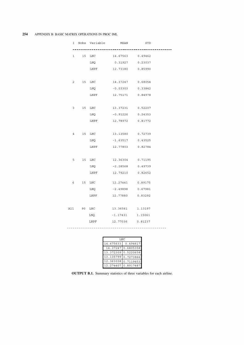
I Nobs Variable MEAN STD
----------------------------------------------------
1 15 LNC 14.67563 0.49462
LNQ 0.31927 0.23037
LNPF 12.73180 0.85990
2 15 LNC 14.37247 0.68054
LNQ –0.03303 0.33842
LNPF 12.75171 0.84978
3 15 LNC 13.37231 0.52207
LNQ –0.91226 0.24353
LNPF 12.78972 0.81772
4 15 LNC 13.13580 0.72739
LNQ –1.63517 0.43525
LNPF 12.77803 0.82784
5 15 LNC 12.36304 0.71195
LNQ –2.28568 0.49739
LNPF 12.79210 0.82652
6 15 LNC 12.27441 0.89175
LNQ -2.49898 0.67981
LNPF 12.77880 0.83292
All 90 LNC 13.36561 1.13197
LNQ -1.17431 1.15061
LNPF 12.77036 0.81237
----------------------------------------------------
LNC
14.675633 0.494617
14.37247 0.6805358
13.372309 0.5220658
13.135799
0.7119453
0.7273866
12.363038
12.274407 0.8917487
OUTPUT B.1. Summary statistics of three variables for each airline.
254 APPENDIX B: BASIC MATRIX OPERATIONS IN PROC IML

Appendix CSIMULATING THE LARGE SAMPLE PROPERTIESOF THE OLS ESTIMATORS
In Chapter 1 we saw that under the least squares assumptions, the estimator b¼ (XTX)�1XTy for the coefficients vector b in the
model y¼XTb þ «was unbiased with variance–covariance matrix given by Var(bjX)¼s2(XTX)�1. Here, s2¼Var(«jX). We
also saw that if «jX�N(0,s2), then the asymptotic distribution of bjX is normal with mean b and variance–covariance
s2(XT
X)�1. That is,bjX�N(b,s2(XTX)�1).This appendixpresents a simple technique for simulating the large sample properties
of the least squares estimator.
Consider the simple linear regression model yi¼ 4 þ 10xi þ «i with one dependent and one explanatory variable. For
simulation purposes, wewill assume that xi�N(10,25) and «i�N(0,2.25). Note that the random nature of the regressor is simply
being used to generate values for the explanatory variable. A single simulation run for this model comprises generating n¼ 50
values of xi and «i, plugging these values into the regression equation to get the corresponding value of the dependent variable, yi.
The simulation ends by running a regression of yi versus xi using the 50 simulated values. Proc Reg is used to estimate the values of
b1,b2, ands2. This simulation is then repeated 10,000 times. Therefore, we end up having 10,000 estimates of the coefficients and
ofs2. ProcMeans is then used to generate basic summary statistics for these 10,000 estimates. The output generated can be used to
determine howclose themeans of the 10,000 sample estimates are to the truevaluesof the parameters (b0¼ 10,b1¼ 4,s2¼ 2.25).
We conducted the simulationwith sample sizes of 50, 100, 500, and 1000. Themeans for the simulation runwith 50 observations is
given in Output C.1. Notice that the sample estimates from the simulation runs are almost identical to the true values.
Hypothesis test on the coefficient b1 was also conducted. We calculated the percentage of times the null hypothesis,
H0: b1¼ 10, was rejected. This gives us an estimate of the true Type I error rate. We used the confidence interval approach for
conducting this test. The tableoutoption ofProcRegwasused to construct the 95%confidence interval forb1. Thenull hypothesis
was rejected if the confidence interval did not include the value under the null hypothesis (10). The output of the simulation run
with 50 observations is given inOutput C.2. It indicates that the null hypothesis is rejected 4.89%of the time, which is close to the
Type I error rate of 5%.
Finally, we use Proc Univariate with the histogram option to generate histograms for different simulation runs to demonstrate
the large sample distribution of b1. The simulation results are given in Figures C.1 – C.4. Notice that the distribution of b1 is bell-
shaped and symmetric evenwhen the sample size is 50. The normality of the distribution becomesmore pronounced as the sample
size increases. Also notice that the spread of the distribution for the estimate reduces as the sample size increases. This indicates
that the standard error of the estimate becomes smaller with increasing sample sizes.
255
Applied Econometrics Using the SAS� System, by Vivek B. AjmaniCopyright � 2009 John Wiley & Sons, Inc.

The following SAS statements can be used to conduct the simulation just described.
data simulation;
sigma=1.5;
beta1=4;
beta2=10;
do index1=1 to 10000;
seed=12345;
do index2=1 to 50;
call rannor(seed,x1);
x=10+5*x1;
e=sigma*normal(0);
y=beta1+beta2*x+e;
output;
end;
end;
run;
proc reg data=simulation noprint outest=estimates tableout;
model y=x;
by index1;
run;
data estimates1;
set estimates;
if y=-1;
rename x=slope;
drop _label_;
run;
proc univariate noprint data=estimates1;
var intercept slope _rmse_;
output out=estimates1 n=n mean=intercept_e slope_e MSE_e;
run;
proc print data=estimates1;
run;
data estimates2;
set estimates;
if _type_ in (’L95B’,’U95B’);
keep index1 _type_ x;
run;
The MEANS ProcedureThe MEANS Procedure
Analysis Variable : reject
N Mean Std Dev Minimum Maximum
10000 0.0497000 0.2173353 0 1.0000000
OUTPUT C.2. Simulated Type 1 error rate (n¼ 50).
Obs n intercept_e slope_e MSE_e
1 10000 4.00117 9.99947 1.49198
OUTPUT C.1. Mean and standard deviation of simulated values of the estimate (n¼ 50).
256 APPENDIX C: SIMULATING THE LARGE SAMPLE PROPERTIES OF THE OLS ESTIMATORS

True Value
9.9 9.93 9.96 9.99 10.02 10.05
0
5
10
15
20
25
30
35
Fitted Normal Distribution of Beta2
Percent
slope
Sample Size 50
The UNIVARIATE ProcedureFitted Distribution for slope
The UNIVARIATE ProcedureFitted Distribution for slope
Parameters for NormalDistribution
Parameter Symbol Estimate
Mean Mu 10
Std Dev Sigma 0.039948
Goodness-of-Fit Tests for Normal Distribution
Test Statistic p Value
Cramer-von Mises W-Sq 0.20979495 Pr > W-Sq 0.223
Anderson-Darling A-Sq 1.21657290 Pr > A-Sq 0.210
Quantiles for NormalDistribution
Quantile
Percent Observed Estimated
1.0 9.89767 9.90707
5.0 9.93906 9.93429
10.0 9.94859 9.94881
25.0 9.96272 9.97306
50.0 9.99712 10.00000
75.0 10.02268 10.02694
90.0 10.05022 10.05119
95.0 10.05629 10.06571
99.0 10.05983 10.09293
FIGURE C.1. Histogram of the simulated estimates (n¼ 50).
APPENDIX C: SIMULATING THE LARGE SAMPLE PROPERTIES OF THE OLS ESTIMATORS 257

True Value
9.915 9.945 9.975 10.005 10.035 10.065 10.095 10.125
0
5
10
15
20
25
30
Percent
slope
Sample Size 100
Fitted Normal Distribution of Beta2
The UNIVARIATE ProcedureFitted Distribution for slope
The UNIVARIATE ProcedureFitted Distribution for slope
Parameters for NormalDistribution
Parameter Symbol Estimate
Mean Mu 10
Std Dev Sigma 0.040671
Goodness-of-Fit Tests for Normal Distribution
Test Statistic p Value
Cramer-von Mises W-Sq 0.12817105 Pr > W-Sq >0.250
Anderson-Darling A-Sq 0.69744815 Pr > A-Sq >0.250
Quantiles for NormalDistribution
Quantile
Percent Observed Estimated
1.0 9.91077 9.90539
5.0 9.93591 9.93310
10.0 9.94713 9.94788
25.0 9.97455 9.97257
50.0 10.00157 10.00000
75.0 10.03171 10.02743
90.0 10.05431 10.05212
95.0 10.06417 10.06690
99.0 10.10230 10.09461
FIGURE C.2. Histogram of the simulated estimates (n¼ 100).
258 APPENDIX C: SIMULATING THE LARGE SAMPLE PROPERTIES OF THE OLS ESTIMATORS

True Value
Fitted Normal Distribution of Beta2
9.84 9.87 9.9 9.93 9.96 9.99 10.02 10.05 10.08 10.11 10.14
0
5
10
15
20
25
30
Percent
slope
Sample Size 500
The UNIVARIATE ProcedureFitted Distribution for slope
The UNIVARIATE ProcedureFitted Distribution for slope
Parameters for NormalDistribution
Parameter Symbol Estimate
Mean Mu 10
Std Dev Sigma 0.044755
Goodness-of-Fit Tests for Normal Distribution
Test Statistic p Value
Cramer-von Mises W-Sq 0.04634466 Pr > W-Sq >0.250
Anderson-Darling A-Sq 0.29383767 Pr > A-Sq >0.250
Quantiles for NormalDistribution
Quantile
Percent Observed Estimated
1.0 9.89798 9.89588
5.0 9.92721 9.92638
10.0 9.94281 9.94264
25.0 9.96843 9.96981
50.0 9.99864 10.00000
75.0 10.02923 10.03019
90.0 10.05702 10.05736
95.0 10.07428 10.07362
99.0 10.10539 10.10412
FIGURE C.3. Histogram of the simulated estimates (n¼ 500).
APPENDIX C: SIMULATING THE LARGE SAMPLE PROPERTIES OF THE OLS ESTIMATORS 259

True Value
Fitted Normal Distribution of Beta2
9.89 9.91 9.93 9.95 9.97 9.99 10.01 10.03 10.05 10.07 10.09 10.11 10.13 10.15
0
2.5
5.0
7.5
10.0
12.5
15.0
17.5
20.0
22.5
Percent
slope
Sample Size 1000
The UNIVARIATE ProcedureFitted Distribution for slope
The UNIVARIATE ProcedureFitted Distribution for slope
Parameters for NormalDistribution
Parameter Symbol Estimate
Mean Mu 10
Std Dev Sigma 0.04417
Goodness-of-Fit Tests for Normal Distribution
Test Statistic p Value
Cramer-von Mises W-Sq 0.14559887 Pr > W-Sq >0.250
Anderson-Darling A-Sq 0.82700450 Pr > A-Sq >0.250
Quantiles for NormalDistribution
Quantile
Percent Observed Estimated
1.0 9.90069 9.89725
5.0 9.92595 9.92735
10.0 9.94106 9.94339
25.0 9.97233 9.97021
50.0 10.00115 10.00000
75.0 10.02828 10.02979
90.0 10.05665 10.05661
95.0 10.07772 10.07265
99.0 10.10588 10.10275
FIGURE C.4. Histogram of the simulated estimates (n¼ 1000).
260 APPENDIX C: SIMULATING THE LARGE SAMPLE PROPERTIES OF THE OLS ESTIMATORS

proc transpose data=estimates2 out=estimates2(keep=L95B U95B);
var x;
id _type_;
by index1;
run;
data estimates2;
set estimates2;
beta2=10;
if L95B<beta2 <U95B then reject=0;else reject=1;
run;
proc means data=estimates2;
var reject;
run;
title ’Fitted Normal Distribution of Beta2’;
proc univariate noprint data=estimates0;
histogram slope /
normal(mu=10 color=blue fill)
cfill = ywh
cframe = ligr
href = 10
hreflabel = ’True Value’
lhref = 2
vaxis = axis1
name = ’MyHist’;
axis1 label=(a=90 r=0);
inset n = ’Sample Size’
beta / pos=ne cfill=ywh;
run;
APPENDIX C: SIMULATING THE LARGE SAMPLE PROPERTIES OF THE OLS ESTIMATORS 261

Appendix DINTRODUCTION TO BOOTSTRAP ESTIMATION
D.1 INTRODUCTION
Bootstrappingisageneral,distribution-freemethodthat isused toestimateparametersofinterest fromdatacollectedfromstudiesor
experiments. It is often referred to as a resamplingmethod because it is carried out by repeatedly drawing samples from the original
data that were gathered. This section introduces the basics of bootstrapping and extends it to bootstrapping in regression analysis.
For a discussion on calculating bias or calculating confidence intervals using bootstrapping, see Efron and Tibshirani (1993).
Bootstrapping is a useful estimation technique when:
1. The formulas that are to be used for calculating estimates are based on assumptions that may not hold or may not be
understood well, or cannot be verified, or are simply dubious.
2. The computational formulas hold only for large samples and are unreliable for small samples or simply not valid for small
samples.
3. The computational formulas do not exist.
To begin the discussion of bootstrapping techniques, assume that a study or experiment was conducted resulting in a data set
x1, . . ., xn of size n. This is a trivial case where the data are univariate in nature. Most studies involve collection of data on several
variables as in the case of regression analysis studies. However,we use the simple example to lay the groundwork for the elements
of bootstrapping methods.
Assume that the data set was generated by some underlying distribution f(u). Here, f(u) is the probability density function and
may be either continuous or discrete. It may be the case that the true density function is unknown and the functional form of f(u) is,
therefore, unknown also. We are interested in estimating the parameter u, which describes some feature of the population from
which the datawere collected. For instance, u could be the truemean,median, the proportion, thevariance, or the standard deviation
of the population. Assume for the moment that we have a well-defined formula to calculate an estimate, u, of u. However, no
formulas exist for calculating the confidence interval for u. Under the ideal setting where we have unlimited resources, we could
draw a large number of samples from the population. We could then estimate u by calculating u for each sample. The calculated
values of u can thenbe used to construct an empirical distribution of u that could then be used to construct a confidence interval for u.
However, in reality we just have a single sample that is a justification for the use of bootstrapping method.
The general idea behind bootstrapping is as follows (assuming that a study/experiment resulted in a data set of size n):
1. A sample of size n is drawn with replacement from the data set in hand.
2. An estimate, u, of u is calculated.
262
Applied Econometrics Using the SAS� System, by Vivek B. AjmaniCopyright � 2009 John Wiley & Sons, Inc.

3. Steps 1 and 2 are repeated several times (sometimes thousands of repetitions are used) to generate a (simulated)
distribution of u. This simulated distribution is then used for making inferences about u.
As an example, suppose that wewant to construct a 95% confidence interval for u. However, we do not have formulas that can
be used for calculating the interval. We can therefore use bootstrapping to construct the confidence interval. The steps are as
follows (Efron and Tibshirani, 1993):
1. Draw1000 (as an example) bootstrap samples from the original data and calculate u1; . . . ; u1000, the estimates from each of
the 1000 samples.
2. Next, sort these estimates in increasing order.
3. Calculate the 2.5th and 97.5th percentile from the 1000 simulated values of u. The 2.5th percentilewill be the average of the
25th and 26th observation while the 97.5th percentile will be the average of the 975th and 976th observation. That is,
Lower confidence limit ¼u25 þ u26
2;
Upper confidence limit ¼u975 þ u976
2:
Notice that we took the lower 2.5% and the upper 2.5% of the simulated distribution of u out to achieve the desired 95%
confidence. Also note that we did notmake any assumptions about the underlying distribution that generated the original data set.
We will now formalize the general bootstrapping method presented so far. Consider a random variable x with cumulative
distribution F(x; u). Here, u is a vector of unknown parameters. For example, if the distribution of x is normal, then u¼ (m, s2).
Assume that we are interested in estimating u or some element of u that describes some aspect of f(x; u), the distribution of x. That
is, wemay be interested in estimating themean, or the standard deviation, or the standard error of themean. Aswe did before, we
will assume that a study/experiment resulted in a random sample x1, . . ., xn of size n. We can use this sample to approximate the
cumulative distribution, F(x; u), with the empirical distribution function, Fðx; uÞ. The estimate, Fðx; uÞ, can be written as
Fðx; uÞ ¼1
n
X
n
i¼1
Ið�1;xÞðxiÞ;
where I is an indicator function that counts the number of x’s in the original sample that fall in the interval (�1, x). This is better
illustrated in Figure D.1.
In Figure D.1, the true distribution, F(x; u), is given by the smooth line while the estimated function, Fðx; uÞ, is given by thestepwise representation. The parameter vector u or elements of it could be calculated exactly if the form ofF(x; u) were known.
FIGURE D.1. Plot comparing actual cumulative versus simulated cumulative distributions. (Graph reproduced with permission from Paul
Glewwe, University of Minnesota.)
APPENDIX D: INTRODUCTION TO BOOTSTRAP ESTIMATION 263

That is, if we knew the exact form of F(x; u), then we could derive the probability density function, f(x; u), or a function t(F) to
calculate u. However, assume that the functional form of F(x; u) is unknown and that it was approximated with Fðx; uÞ.Therefore, one option we have is to replace F(x; u) with Fðx; uÞ to get the estimated function tðFÞ. We can then use tðFÞto calculate an estimate, u, of u. The estimator u in this instance is called the plug-in estimator of u (Efron and Tibshirani, 1993,
p. 35). As an example, the plug-in estimator of the population mean mx,
mx ¼
ð
1
�1
xf ðxÞ dx;
is the sample mean
�x ¼1
n
X
n
i¼1
xi:
Notice that calculating the mean of x was trivial and did not require bootstrapping methods. In general, bootstrapping
techniques are used to calculate standard errors and for constructing confidence intervals without making any assumption
about the underlying distribution from which the samples are drawn.
D.2 CALCULATING STANDARD ERRORS
We will now discuss how bootstrapping methods can be used to calculate an estimate of the standard error of the parameter of
interest. Assume then that we have an estimate of u. That is, u was calculated from the original data set without the use of
bootstrapping. Bootstrapping, however, will be used to calculate an estimate of the standard error of u. The general method for
doing this is as follows (again assume that we have a data set of size n) (Efron and Tibshirani, 2004, p. 45):
1. Draw B samples of size n with replacement from the original data set.
2. Calculate u for each of the samples from step 1. That is, we now have u1; . . . ; uB.
3. We calculate the standard error from the B estimates of u by using the standard formulas for standard errors. That is,
seBðuÞ ¼
ffiffiffiffiffiffiffiffiffiffiffiffiffiffiffiffiffiffiffiffiffiffiffiffiffiffiffiffiffiffiffiffiffi
1
B�1
X
B
i¼1
ðui��uÞ2
v
u
u
t
;
where�u ¼ B�1
P
B
i¼1
ui is simply the mean of the u1; . . . ; uB. In practice, B is set to a very large number. Most practitioners
use 200–500 bootstrapped samples.
D.3 BOOTSTRAPPING IN SAS
Bootstrapping can easily be programmed in SAS by using simple routines. SAS macros to calculate bootstrapped estimates are
available for download from the SAS Institute. The macros can be used to calculate bootstrapped and jackknife estimates for the
standard deviation and standard error, and they are also used to calculate the bootstrapped confidence intervals. The macros can
also be used to calculate bootstrapped estimates of coefficients in regression analysis. These macros need to be invoked from
withinSAS.Wewill illustrate theuseof thesemacros abit later. Fornow,weshowhowasimpleprogramcanbewritten to compute
bootstrap estimates.
Consider a data set that consists of 10 values: 196,�12, 280, 212, 52, 100,�206, 188,�100, 202.Wewill calculate bootstrap
estimates of the standard error for the mean. The following SAS statements can be used:
data age_data;
input age;
cards;
45
264 APPENDIX D: INTRODUCTION TO BOOTSTRAP ESTIMATION

40
9
7
17
16
15
11
10
8
54
76
87
;
data bootstrap;
do index=1 to 500;
do i=1 to nobs;
x=round(ranuni(0)*nobs);
set age_data
nobs=nobs
point=x;
output;
end;
end;
stop;
run;
The following Proc Univariate statements will calculate the mean of the bootstrapped samples.
proc univariate data=bootstrap noprint;
var age;
by index;
output out=out1 mean=mean n=n;
run;
Finally, the following Proc Univariate statements will calculate the standard deviation of the 500 bootstrapped means.
proc univariate data=out1 noprint;
var mean;
output out=out2 n=n mean=mean std=se;
run;
proc print data=out2;
run;
The analysis results in a mean and standard error of 27.6 and 6.8, respectively.
D.4 BOOTSTRAPPING IN REGRESSION ANALYSIS
Consider the standard linear regressionmodelyi ¼ xTi bþ «i,wherexiandb arek� 1columnvectors and ei is randomerror.Assume
that we have a data set comprising n pairs of observations (y1, x1), . . ., (yn, xn). Assume that the conditional expectation
E(«ijxi)¼ 0.Furthermore, assume thatwedonot knowF(«jx), the cumulativedistributionofe. Ingeneral,F is assumed tobenormal.
APPENDIX D: INTRODUCTION TO BOOTSTRAP ESTIMATION 265

Wewill make use the standard least squares estimator for b, namely, b ¼ ðXTXÞ�1XTy, to calculate bootstrapped estimates.
That is, as was the case, with the mean being calculated without the use of bootstrapping, we will assume that the least squares
estimate can be calculated without any need of bootstrapping. However, we are interested in calculating the standard errors of b.
That is, we assume that the formulas for calculating the standard errors are either unknown, unreliable, or simply do not work for
small samples.
As shown in Chapter 1, the estimate of the variance of b is VarðbjXÞ ¼ s2ðXTXÞ�1, where s2 is estimated as
s2 ¼1
n
X
n
i¼1
ðyi�xTi bÞ2
or
s2 ¼1
n�k�1
X
n
i¼1
ðyi�xTi bÞ2:
Notice that the first version is not an unbiased estimator fors2whereas the second version is. These versions are often referred
to as the “not bias-corrected” and the “bias-corrected” versions, respectively. There are two bootstrappedmethods (pairsmethod,
residuals method) that are employed to estimate the standard error of b (Glewwe, 2006; Efron and Tibshirani, 1993, p. 113).
The bootstrapped pairs method randomly selects pairs of yi and xi to calculate an estimate of «i, while the bootstrapped
residuals method takes each xi just once but then links it with a random draw of an estimate of e. The next section outlines both
methods.
D.4.1 Bootstrapped Residuals Method
As before, we assume that a study or experiment resulted in n observations (y1, x1), . . ., (yn, xn). The general method for the
bootstrapped residuals method is
1. For each i, calculate an estimate, ei of «i. That is, ei ¼ yi � xTi b where b is the usual OLS estimator calculated from the
original data.
2. Randomly draw n values of ei (from step 1) with replacement. Denote the residuals in the sample as e�1; e�2; . . . ; e
�n. Notice
that the subscripts of the residuals in the selected sample are not the same as the subscripts for the residuals, ei, which were
calculated from the original sample. That is, in general e�i 6¼ ei for i¼ 1, . . ., n.
3. With the values of e�i (from step 2), compute y�i ¼ xTi bþ e�i . Notice that the subscripts for xi herematch the subscripts of xiin the original data set. That is, we are using each xi only once. Notice also that by construction of e�i , yi 6¼ y�i .
4. Using the calculated values of y�i (from step 3), construct the vector y*. Finally, use X ¼ x1 . . . xn �T
�
and
y� ¼ y�1 . . . y�n �T
�
to calculate b�1, the first bootstrapped estimate of b. That is, b�
1 ¼ ðXTXÞ�1XTy�.
5. Steps 2 through 4 are repeated B (typically B¼ 200–500) times to get B estimates of b.
6. Use the B estimates (from step 5) to calculate the sample standard deviation of b using the formula
s:e:� ¼
ffiffiffiffiffiffiffiffiffiffiffiffiffiffiffiffiffiffiffiffiffiffiffiffiffiffi
P
B
i¼1
ðb�
i�b�Þ2
B�1
v
u
u
u
t
;
where
b�¼
1
B
X
B
i¼1
b�
i
is the mean of the B residuals method bootstrapped estimates of b.
266 APPENDIX D: INTRODUCTION TO BOOTSTRAP ESTIMATION

D.4.2 Bootstrapped Pairs Method
As before, we assume that a study or experiment resulted in n observations (y1, x1), . . ., (yn, xn). The general method for the
bootstrapped pairs method is
1. Randomly draw n pairs of values, yi and xi, with replacement. Denote these as y�1; y�2; . . . ; y
�n and x�1; x
�2; . . . ; x
�n. As
discussed earlier, the subscripts here do not necessarily match the subscripts in the original data set.
2. Using these values of y�i and x�i , calculate the first bootstrapped estimate of b by using standard OLS techniques. That is,
b�1 ¼ ðX�TX�Þ�1X�Ty�.
3. Steps 1 and 2 are repeated B times (typically B¼ 200–500) to get B estimates of b.
4. Use the B estimates b�i ; i ¼ 1; . . . ;B, to calculate the sample standard deviation of b using the formula
s:e:� ¼
ffiffiffiffiffiffiffiffiffiffiffiffiffiffiffiffiffiffiffiffiffiffiffiffiffi
P
B
i¼1
ðb�i�b�Þ2
B�1
v
u
u
u
t
;
where
b�¼
1
B
X
B
i¼1
b�i
is the mean of the B pairs method bootstrapped estimates of b. Computationally, the bootstrapped pairs method is more
straightforward. As discussed in Efron and Tibshirani (1993, p. 113), the bootstrapped residuals method imposes
homoscedasticity because it “delinks” xiwith ei. Therefore, if the homoscedasticity assumption is violated, thenwe should
use the bootstrapped pairs method, which does not impose this. On the other hand, if we are very confident of
homoscedasticity, then we can use the bootstrapped residuals method to get more precise estimates of the standard error
of b. In fact, it can be shown that as B ! 1 the standard errors of the least squares estimates calculated using the
bootstrapped residuals method converge to the diagonal elements of the variance–covariance matrix s2ðXTXÞ�1.
D.4.3 Bootstrapped Regression Analysis in SAS
Wewill now illustrate the residuals and the pairs methods by using the %BOOT macro that can be downloaded from the SAS
Institute website at www.sas.com. We will make use of the gasoline consumption data given in Table F2.1 of Greene (2003).
We need the bootstrapped macros (labeled JACKBOOT.SAS here) to be called from within the program. The %include
statement can be used for this purpose. The following statements can be used:
%include "C:\Temp\jackboot.sas";
The data set is then read into SAS and stored into a temporary SAS data set called gasoline. Notice that the raw data are stored
in Excel format.
proc import out=gasoline
datafile="C:\Temp\gasoline"
dbms=Excel Replace;
getnames=yes;
run;
The following SAS data step statements simply transform the variables in the raw data by using the log transformations:
data gasoline;
set gasoline;
Ln_G_Pop=log(G/Pop);
APPENDIX D: INTRODUCTION TO BOOTSTRAP ESTIMATION 267

Ln_pg=Log(Pg);
Ln_Income=Log(Y/Pop);
Ln_Pnc=Log(Pnc);
Ln_Puc=Log(Puc);
run;
The followingProcRegstatements are used to runOLSregressionon theoriginal data set.The residuals from this are stored in a
temporary SAS data set called gasoline. The residuals are labeled as resid.
proc reg data=gasoline;
model Ln_G_Pop=Ln_pg Ln_Income Ln_Pnc Ln_Puc;
output out=gasoline r=resid p=pred;
run;
The following macro is required before invoking the bootstrapped macros in the program jackboot.sas. The only inputs that
require changes are the variable names in the model statement. The remaining statements can be used as is. See Sample 24982-
JackKnife and Bootstrap Analyses from the SAS Institute for more details. The following code has been adapted from this
publication and has been used with permission from the SAS Institute.
%macro analyze(data=,out=);
options nonotes;
proc reg data=&data noprint
outest=&out(drop=Y _IN_ _P_ _EDF_);
model Ln_G_Pop=Ln_pg Ln_Income Ln_Pnc Ln_Puc;
%bystmt;
run;
options notes;
%mend;
This portion of the code invokes the%boot macrowithin jackboot.sas and conducts a bootstrapped analysis by using the pairs
method.Note that the rootmean square error (_RMSE_) is not a plug-in estimator fors, and therefore the bias correction iswrong.
In otherwords, even though themean square error is unbiased fors2, the rootmean square error is not unbiased fors.However,we
choose to ignore this because the bias is minimal.
title2 ’Resampling Observations-Pairs Method’;
title3 ’(Bias correction for _RMSE_ is wrong)’;
%boot(data=gasoline, random=123);
This portion of the code invokes the %boot macro and conducts the bootstrapped analysis by using the residuals method.
title2 ’Resampling Residuals-Residual Method’;
title3 ’(bias correction for _RMSE_ is wrong)’;
%boot(data=gasoline, residual=resid, equation=y=pred+resid,
random=123);
Theanalysis results aregiven inOutputsD.1 andD.2.The first part of theoutput is from theanalysis of theoriginal data.Wewill
skip anydiscussion of this portion of the output aswe have already discussedOLS regression output fromSAS in detail inChapter
2. TheOLS output is followed by the outputwhere bootstrapping is done by resampling pairs (OutputD.1) andwhere the analysis
was done using the residuals method (Output D.2).
268 APPENDIX D: INTRODUCTION TO BOOTSTRAP ESTIMATION

The REG ProcedureModel: MODEL1
Dependent Variable: Ln_G_Pop
The REG ProcedureModel: MODEL1
Dependent Variable: Ln_G_Pop
Number of Observations Read 36
Number of Observations Used 36
Analysis of Variance
Source DFSum ofSquares
MeanSquare F Value Pr > F
Model 4 0.78048 0.19512 243.18 <0.0001
Error 31 0.02487 0.00080237
Corrected Total 35 0.80535
Root MSE 0.02833 R-Square 0.9691
Dependent Mean –0.00371 Adj R-Sq 0.9651
Coeff Var –763.79427
Parameter Estimates
Variable DFParameterEstimate
StandardError t Value Pr > |t|
Intercept 1 –7.78916 0.35929 –21.68 <0.0001
Ln_pg 1 –0.09788 0.02830 -3.46 0.0016
Ln_Income 1 2.11753 0.09875 21.44 <0.0001
Ln_Pnc 1 0.12244 0.11208 1.09 0.2830
Ln_Puc 1 –0.10220 0.06928 –1.48 0.1502
Resampling Observations(bias correction for _RMSE_ is wrong)
Resampling Observations(bias correction for _RMSE_ is wrong)
Resampling Observations(bias correction for _RMSE_ is wrong)
Resampling Observations(bias correction for _RMSE_ is wrong)
NameObservedStatistic
BootstrapMean
ApproximateBias
ApproximateStandardError
ApproximateLower
ConfidenceLimit
Bias-CorrectedStatistic
Intercept –7.78916 –7.83880 –0.049634 0.35056 –8.42662 –7.73953
Ln_G_Pop –1.00000 –1.00000 0.000000 0.00000 –1.00000 –1.00000
Ln_Income 2.11753 2.13101 0.013484 0.09596 1.91597 2.10405
Ln_Pnc 0.12244 0.13541 0.012969 0.13611 –0.15729 0.10947
Ln_Puc –0.10220 –0.11723 –0.015028 0.08629 –0.25631 –0.08718
Ln_pg –0.09788 –0.09167 0.006209 0.02904 –0.16101 –0.10409
_RMSE_ 0.02833 0.02623 –0.002093 0.00256 0.02540 0.03042
Name
ApproximateUpper
ConfidenceLimit
ConfidenceLevel (%)
Method forConfidenceInterval
MinimumResampledEstimate
MaximumResampledEstimate
Number ofResamples
LABEL OF FORMERVARIABLE
Intercept –7.05244 95 Bootstrap Normal –8.98495 –7.03140 200 Intercept
Ln_G_Pop –1.00000 95 Bootstrap Normal –1.00000 –1.00000 200
Ln_Income 2.29212 95 Bootstrap Normal 1.90256 2.44562 200
Ln_Pnc 0.37624 95 Bootstrap Normal –0.23416 0.42458 200
Ln_Puc 0.08196 95 Bootstrap Normal –0.32506 0.10206 200
Ln_pg –0.04717 95 Bootstrap Normal –0.16467 0.00233 200
_RMSE_ 0.03544 95 Bootstrap Normal 0.01844 0.03362 200 Root mean squared error
OUTPUT D.1. Bootstrapped regression analysis (pairs method) of the gasoline consumption data.
APPENDIX D: INTRODUCTION TO BOOTSTRAP ESTIMATION 269

The REG ProcedureModel: MODEL1
Dependent Variable: Ln_G_Pop
The REG ProcedureModel: MODEL1
Dependent Variable: Ln_G_Pop
Number of Observations Read 36
Number of Observations Used 36
Analysis of Variance
Source DFSum ofSquares
MeanSquare F Value Pr > F
Model 4 0.78048 0.19512 243.18 <0.0001
Error 31 0.02487 0.00080237
Corrected Total 35 0.80535
Root MSE 0.02833 R-Square 0.9691
Dependent Mean –0.00371 Adj R-Sq 0.9651
Coeff Var –763.79427
Parameter Estimates
Variable DFParameterEstimate
StandardError t Value Pr > |t|
Intercept 1 –7.78916 0.35929 –21.68 <0.0001
Ln_pg 1 –0.09788 0.02830 –3.46 0.0016
Ln_Income 1 2.11753 0.09875 21.44 <0.0001
Ln_Pnc 1 0.12244 0.11208 1.09 0.2830
Ln_Puc 1 –0.10220 0.06928 –1.48 0.1502
NameObservedStatistic
BootstrapMean
ApproximateBias
ApproximateStandardError
ApproximateLower
ConfidenceLimit
Bias-CorrectedStatistic
Intercept –7.78916 –7.78916 2.30926E-14 0 –7.78916 –7.78916
Ln_G_Pop –1.00000 –1.00000 0 0 –1.00000 –1.00000
Ln_Income 2.11753 2.11753 4.44089E-15 0 2.11753 2.11753
Ln_Pnc 0.12244 0.12244 2.22045E-16 0 0.12244 0.12244
Ln_Puc –0.10220 –0.10220 1.38778E-16 0 –0.10220 –0.10220
Ln_pg –0.09788 –0.09788 –1.6653E-16 0 –0.09788 –0.09788
_RMSE_ 0.02833 0.02833 4.85723E-17 0 0.02833 0.02833
Name
ApproximateUpper
ConfidenceLimit
ConfidenceLevel (%)
Method forConfidenceInterval
MinimumResampledEstimate
MaximumResampledEstimate
Number ofResamples
LABEL OF FORMERVARIABLE
Intercept –7.78916 95 Bootstrap Normal –7.78916 –7.78916 200 Intercept
Ln_G_Pop –1.00000 95 Bootstrap Normal –1.00000 –1.00000 200
Ln_Income 2.11753 95 Bootstrap Normal 2.11753 2.11753 200
Ln_Pnc 0.12244 95 Bootstrap Normal 0.12244 0.12244 200
Ln_Puc –0.10220 95 Bootstrap Normal –0.10220 –0.10220 200
Ln_pg –0.09788 95 Bootstrap Normal –0.09788 –0.09788 200
_RMSE_ 0.02833 95 Bootstrap Normal 0.02833 0.02833 200 Root mean squared error
Resampling Residuals(bias correction for _RMSE_ is wrong)(bias correction for _RMSE_ is wrong)
OUTPUT D.2. Bootstrapped regression analysis (residuals method) of the gasoline consumption data.
270 APPENDIX D: INTRODUCTION TO BOOTSTRAP ESTIMATION

The output consists of the OLS estimates in the first column, followed by the mean of the coefficients estimated from the 200
bootstrap samples. The third columngives the bias,which is simply the bootstrapmeanminus the observed statistic. The standard
errors calculated from the bootstrapped samples are given next. This is followed by the 95% confidence intervals, the bias-
corrected statistics, and the minimum and maximum of the estimated coefficient values from the bootstrap samples. Notice that
the bootstrap estimates of the coefficients and the standard errors are very similar to the OLS estimates.
There is a remarkable similarity between the bootstrap estimates of the coefficients and the standard errors obtained from the
residual method and the OLS estimates. This is not surprising since under the homoscedastic assumption, it can be shown that as
the number of bootstrapped samples increases, the estimated values of the standard errors converge to the diagonal elements of
sðXTXÞ�1, where s2 is the estimate that is not corrected for bias.
APPENDIX D: INTRODUCTION TO BOOTSTRAP ESTIMATION 271

Appendix ECOMPLETE PROGRAMS AND PROC IML ROUTINES
E.1 PROGRAM 1
This programwasused inChapter 2. It is used to analyzeTableF3.1ofGreene (2003). In the followingdata step,we read in the raw
data, create a trend variable, T, divide GNP and Invest by CPI, and then scale the transformed GNP and Invest time series so that
they are measured in trillions of dollars.
proc import out=invst_equation
datafile="C:\Temp\Invest_Data"
dbms=Excel Replace;
getnames=yes;
run;
data invst_equation;
set invst_equation;
T=_n_;
Real_GNP=GNP/(CPI*10);
Real_Invest=Invest/(CPI*10);
run;
/* The start of Proc IML routines.
*/proc iml;
/* Invoke Proc IML and create the X and Y matrices using the variables T, Real_GNP, and
Real_Invest from the SAS data set invst_equation. */
use invst_equation;
read all var {’T’ ’Real_GNP’} into X;
read all var {’Real_Invest’} into Y;
/* Define the number of observations and the number of independent variables. */
n=nrow(X);
k=ncol(X);
/* Create a column of ones to the X matrix to account for the intercept term. */
X=J(n,1,1)||X;
272
Applied Econometrics Using the SAS� System, by Vivek B. AjmaniCopyright � 2009 John Wiley & Sons, Inc.

/* Calculate the inverse of X’X and use this to compute B_Hat */
C=inv(X`*X);
B_Hat=C*X`*Y;
/* Compute SSE, the residual sum of squares, and MSE, the residual mean square. */
SSE=y`*y-B_Hat *X`*Y;
DFE=n-k-1;
MSE=sse/DFE;
/* Compute SSR, the sums of squares due to the model; MSR, the sums of squares due to random
error; and the F ratio. */
Mean_Y=Sum(Y)/n;
SSR=B_Hat *X`*Y-n*Mean_Y**2;
MSR=SSR/k;
F=MSR/MSE;
/* Compute R-Square and Adj-RSquare. */
SST=SSR+SSE;
R_Square=SSR/SST;
Adj_R_Square=1-(n-1)/(n-k) * (1-R_Square);
/* Compute the standard error of the parameter estimates, their T statistic and P-values. */
SE=SQRT(vecdiag(C)#MSE);
T=B_Hat/SE;
PROBT=2*(1-CDF(’T’, ABS(T), DFE));
/* Concatenate the results into one matrix to facilitate printing. */
Source=(k||SSR||MSR||F)//(DFE||SSE||MSE||{.});
STATS=B_Hat||SE||T||PROBT;
Print ’Regression Results for the Investment Equation’;
Print Source (|Colname={DF SS MS F} rowname={Model Error} format=8.4|);
Print ’Parameter Estimates’;
Print STATS (|Colname={BHAT SE T PROBT} rowname={INT T G _R_ P}format=8.4|);
Print ’’;
Print ’The value of R-Square is ’ R_Square;
Print ’The value of Adj R-Square is ’ Adj_R_Square;
run;
E.2 PROGRAM 2
This program was used in Chapter 3. It analyzes the quarterly data on investment as found in Table 5.1 of Greene (2003). This
program is used to conduct the general linear hypothesis—the global F test. We have omitted the data step statements with the
hope that users will be able to recreate it with ease. The Proc IML code follows.
proc iml;
/* Invoke Proc IML and create the X and Y matrices using the variables Invest, Interest,
delta_p, output, and T from the SAS data set real_invst_eq (Notice we have omitted the data
step) */
use real_invst_eq;
read all var {’interest’ ’delta_p’ ’output’ ’T’} into X;
read all var {’Invest’} into Y;
/* Define the number of observations and the number of independent variables. */
n=nrow(X);
k=ncol(X);
/* Create a column of ones to the X matrix to account for the intercept term. */
X=J(n,1,1)||X;
/* Calculate the inverse of X’X and use this to compute B_Hat. */
C=inv(X`*X);
APPENDIX E: COMPLETE PROGRAMS AND PROC IML ROUTINES 273

B_Hat=C*X`*Y;
/* Construct the R Matrix and q matrix. */
R={0 1 1 0 0,0 0 0 1 0,0 0 0 0 1};
q={0,1,0};
j=nrow(R);
/* Compute SSE, the residual sum of squares, and MSE, the residual mean square. */
SSE=y`*y-B_Hat *X`*Y;
DFE=n-k-1;
MSE=sse/DFE;
/* Calculate the F Statistic. */
DisVec=R*B_Hat-q;
F=DisVec`*inv(R*MSE*C*R`)*DisVec/j;
P=1-ProbF(F,J,n-k);
Print ’The value of the F Statistic is ’ F;
Print ’The P-Value associated with this is ’ P;
run
E.3 PROGRAM 3
This programwasused inChapter 3. Itwasused to analyze the investment equationdata given inTableF5.1ofGreene (2003).This
program calculates the restricted least squares estimator and the standard errors of the estimator. We have omitted the data step
again.
proc iml;
/* Invoke Proc IML and create the X and Y matrices using the variables Invest, Interest,
delta_p, output, and T from the SAS data set real_invst_eq. */
use real_invst_eq;
read all var {’interest’ ’delta_p’ ’output’ ’T’} into X;
read all var {’Invest’} into Y;
/* Define the number of observations and the number of independent variables. */
n=nrow(X);
k=ncol(X);
/* Create a column of ones to the X matrix to account for the intercept term. */
X=J(n,1,1)||X;
/* Calculate the inverse of X’X and use this to compute B_Hat. */
C=inv(X`*X);
B_Hat=C*X`*Y;
/* Construct the R matrix and q matrix. */
R={0 1 1 0 0};
q={0};
/* Calculate the Restricted Least Squares Estimator. */
M=R‘*inv(R*C*R‘)*(R*B_Hat-q);
B_Star=B_Hat - C*M;
print B_Star;
/* Compute SSE, and MSE. */
SSE=y`*y-B_Hat *X`*Y;
DFE=n-k-1;
MSE=sse/DFE;
/* Compute SSR, MSR, and the F statistic. */
Mean_Y=Sum(Y)/n;
SSR=B_Hat *X`*Y-n*Mean_Y**2;
MSR=SSR/k;
274 APPENDIX E: COMPLETE PROGRAMS AND PROC IML ROUTINES

F=MSR/MSE;
/* Compute R-Square and Adj-RSquare. */
SST=SSR+SSE;
R_Square=SSR/SST;
Adj_R_Square=1-(n-1)/(n-k) * (1-R_Square);
/* Compute the standard error of the parameter estimates, their T statistic and P-values. */
SE=SQRT(vecdiag(C)#MSE);
T=B_Hat/SE;
PROBT=2*(1-CDF(’T’, ABS(T), DFE));
/* Concatenate the results into one matrix. */
Source=(k||SSR||MSR||F)//(DFE||SSE||MSE||{.});
STATS=B_Hat||SE||T||PROBT;
Print ’Regression Results for the Restricted Investment Equation’;
Print Source (|Colname={DF SS MS F} rowname={Model Error} format=8.4|);
Print ’Parameter Estimates’;
Print STATS (|Colname={BHAT SE T PROBT} rowname={INT Interest
Delta_P Output T} format=8.4|);
Print ’’;
Print ’The value of R-Square is ’ R_Square;
Print ’The value of Adj R-Square is ’ Adj_R_Square;
run;
E.4 PROGRAM 4
This program was used in Chapter 3 to conduct general linear hypothesis for the investment equation data given in Table F5.1 of
Greene (2003). Note that Program 2 simply conducts the globalF test, whereas this program does the individual t tests for each of
the linear restrictions.
proc iml;
/* Invoke Proc IML and create the X and Y matrices using the variables Invest, Interest,
delta_p, output, and T from the SAS data set real_invst_eq. */
use real_invst_eq;
read all var {’interest’ ’delta_p’ ’output’ ’T’} into X;
read all var {’Invest’} into Y;
/* Define the number of observations and the number of independent variables. */
n=nrow(X);
k=ncol(X);
/* Create a column of ones to the X matrix to account for the intercept term. */
X=J(n,1,1)||X;
/* Calculate the inverse of X’X and use this to compute B_Hat. */
C=inv(X`*X);
B_Hat=C*X`*Y;
/* Construct the R Matrix and q matrix. */
R={0 1 1 0 0,0 0 0 1 0,0 0 0 0 1};
q={0,1,0};
j=nrow(R);
R1=R[1,];q1=q[1,];
R2=R[2,];q2=q[2,];
R3=R[3,];q3=q[3,];
/* Compute SSE, and MSE. */
SSE=y`*y-B_Hat *X`*Y;
APPENDIX E: COMPLETE PROGRAMS AND PROC IML ROUTINES 275

DFE=n-k-1;
MSE=sse/DFE;
/* Calculate the t Statistic. */
T_NUM1=R1*B_Hat-q1;
se1=sqrt(R1*MSE*C*R1‘);
T1=T_NUM1/se1;
p1=1-ProbT(T1,n-k);
Print ’The value of the T Statistic for the first restriction is ’ t1;
Print ’The P-Value associated with this is ’ P1;
T_NUM2=R2*B_Hat-q2;
se2=sqrt(R2*MSE*C*R2‘);
T2=T_NUM2/se2;
P2=1-ProbT(T2,n-k);
Print ’The value of the T Statistic for the second restriction is ’ t2;
Print ’The P-Value associated with this is ’ P2;
T_NUM3=R3*B_Hat-q3;
se3=sqrt(R3*MSE*C*R3`);
T3=T_NUM3/se3;
P3=1-ProbT(T3,n-k);
Print ’The value of the T Statistic for the third restriction is ’ t3;
Print ’The P-Value associated with this is ’ P3;
run;
E.5 PROGRAM 5
This program was used in Chapter 4 to conduct Hausman�s specification test on the consumption data that can be found in
Table 5.1 of Greene (2003). We have chosen to omit the data step statements.
proc iml;
/* Read the data into appropriate matrices. */
use hausman;
read all var {’yt’ ’it’ ’ct1’} into X;
read all var {’ct’} into Y;
/* Create the instruments matrix Z and some constants. */
read all var {’it’ ’ct1’ ’yt1’} into Z;
n=nrow(X);
k=ncol(X);
X=J(n,1,1)||X;
Z=J(n,1,1)||Z;
/* Calculate the OLS and IV estimators. */
CX=inv(X`*X);
CZ=inv(Z`*Z);
OLS_b=CX*X`*y;
Xhat=Z*CZ*Z‘*X;
b_IV=inv(Xhat`*X)*Xhat *y;
/* Calculate the difference between the OLS and IV estimators. Also, calculate MSE */
d=b_IV-OLS_b;
SSE=y`*y-OLS_b`*X`*Y;
DFE=n-k;
MSE=sse/DFE;
/* Calculate the GINVERSE of the difference inv(X`*X) - inv(Xhat`*Xhat). */
276 APPENDIX E: COMPLETE PROGRAMS AND PROC IML ROUTINES

/* Calculate the Hausman’s test statistic. */
diff=ginv(inv(Xhat`*Xhat)-CX);
H=d`*diff*d/mse;
J=round(trace(ginv(diff)*diff));
Table=OLS_b||b_IV;
Print Table (|Colname={OLS IV} rowname={Intercept yt it ct1} format=8.4|);
Print ’The Hausman Test Statistic Value is ’ H;
run;
E.6 PROGRAM 6
This program was used in Chapter 5 to calculate the estimates of the robust variance–covariance matrices under
heteroscedasticity. The analysis is done on the credit card data found in Table 9.1 of Greene (2003). The code calculates
White�s estimator and the two alternatives proposed by David and MacKinnon.
proc iml;
/* Read the data into matrices and create constants. */
use Expense;
read all var {’age’ ’ownrent’ ’income’ ’incomesq’} into X;
read all var {’avgexp’} into Y;
n=nrow(X);
X=J(n,1,1)||X;
k=ncol(X);
/* Calculate the inverse of X’X.*/
C=inv(X`*X);
/* Calculate the least squares estimator, beta_hat. */
beta_hat=C*X`*y;
/* Calculate the residuals and MSE. */
resid=y-X*beta_hat;
SSE=y`*y-beta_hat`*X`*Y;
MSE=sse/(n-k);
/* Calculate the S0 term of White’s Estimator. */
/* First, initialize a n by n matrix with zero’s. */
S0=J(k,k,0);
do i=1 to n;
S0=S0 + resid[i,]*resid[i,]*X[i,]`*X[i,];
end;
S0=S0/n;
/* Now, calculate White’s Estimator. */
White=n*C*S0*C;
/* Now, calculate the first recommendation of David & MacKinnon for White’s estimator. */
DM1=n/(n-k) * White;
/* Now, calculate the second recommendation of David & MacKinnon for White’s estimator. */
S0=J(k,k,0);
do i=1 to n;
m_ii=1-X[i,]*C*X[i,]`;
Temp_Ratio=resid[i,]*resid[i,]/m_ii;
S0=S0+Temp_Ratio*X[i,]‘*X[i,];
end;
S0=S0/n;
/* Now, calculate the modified White’s Estimator. */
DM2=n*C*S0*C;
APPENDIX E: COMPLETE PROGRAMS AND PROC IML ROUTINES 277
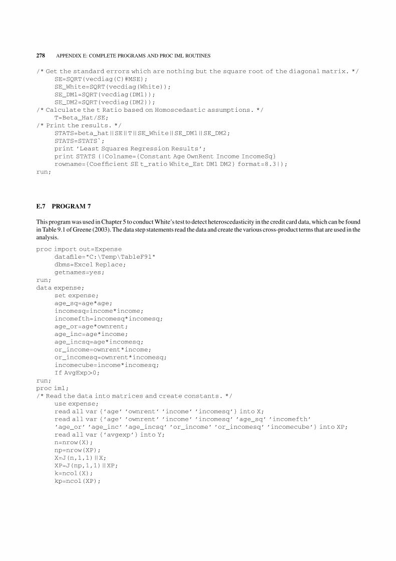
/* Get the standard errors which are nothing but the square root of the diagonal matrix. */
SE=SQRT(vecdiag(C)#MSE);
SE_White=SQRT(vecdiag(White));
SE_DM1=SQRT(vecdiag(DM1));
SE_DM2=SQRT(vecdiag(DM2));
/* Calculate the t Ratio based on Homoscedastic assumptions. */
T=Beta_Hat/SE;
/* Print the results. */
STATS=beta_hat||SE||T||SE_White||SE_DM1||SE_DM2;
STATS=STATS`;
print ’Least Squares Regression Results’;
print STATS (|Colname={Constant Age OwnRent Income IncomeSq}
rowname={Coefficient SE t_ratio White_Est DM1 DM2} format=8.3|);
run;
E.7 PROGRAM 7
This programwas used inChapter 5 to conductWhite�s test to detect heteroscedasticity in the credit card data, which can be found
inTable 9.1 ofGreene (2003). The data step statements read the data and create thevarious cross-product terms that are used in the
analysis.
proc import out=Expense
datafile="C:\Temp\TableF91"
dbms=Excel Replace;
getnames=yes;
run;
data expense;
set expense;
age_sq=age*age;
incomesq=income*income;
incomefth=incomesq*incomesq;
age_or=age*ownrent;
age_inc=age*income;
age_incsq=age*incomesq;
or_income=ownrent*income;
or_incomesq=ownrent*incomesq;
incomecube=income*incomesq;
If AvgExp>0;
run;
proc iml;
/* Read the data into matrices and create constants. */
use expense;
read all var {’age’ ’ownrent’ ’income’ ’incomesq’} into X;
read all var {’age’ ’ownrent’ ’income’ ’incomesq’ ’age_sq’ ’incomefth’
’age_or’ ’age_inc’ ’age_incsq’ ’or_income’ ’or_incomesq’ ’incomecube’} into XP;
read all var {’avgexp’} into Y;
n=nrow(X);
np=nrow(XP);
X=J(n,1,1)||X;
XP=J(np,1,1)||XP;
k=ncol(X);
kp=ncol(XP);
278 APPENDIX E: COMPLETE PROGRAMS AND PROC IML ROUTINES

/* First get the residuals from OLS. */
C=inv(X`*X);
beta_hat=C*X`*y;
resid=y-X*beta_hat;
/* Square the residuals for a regression with cross product terms in White’s test. */
resid_sq=resid#resid;
/* Regress the square of the residuals versus the 13 variables in X. */
C_E=inv(XP`*XP);
b_hat_e=C_E*XP`*resid_sq;
/* Calculate R-Square from this regression. */
Mean_Y=Sum(resid_sq)/np;
SSR=b_hat_e`*XP`*resid_sq-np*Mean_Y**2;
SSE=resid_sq`*resid_sq-b_hat_e`*XP`*resid_sq;
SST=SSR+SSE;
R_Square=SSR/SST;
print R_Square;
/* Calculate and print the test statistic value and corresponding p-value. */
White=np*R_Square;
pvalue= 1 - probchi(White, kp);
print ’The test statistic value for Whites Test is ’White;
print ’The p-value associated with this test is ’pvalue;
run;
E.8 PROGRAM 8
This programwas used in Chapter 5 to conduct the Breusch-Pagan LagrangeMultiplier test on the credit card data, which can be
found in Table 9.1 of Greene (2003). Note that we have omitted the data step statements.
proc iml;
/* Read the data into matrices and prep matrices for analysis. */
use expense;
read all var {’age’, ’ownrent’,’income’,’incomesq’ } into X;
read all var {’income’, ’incomesq’ } into Z;
read all var {’avgexp’ } into y;
/* Create a few constants. */
n=nrow(X);
X=J(n,1,1)||X;
Z=J(n,1,1)||Z;
/* Calculate the residuals from OLS. */
bhat_OLS=inv(X‘*X)*X`*y;
SSE=(y-X*bhat_OLS)‘*(y-X*bhat_OLS);
resid=y-X*bhat_OLS;
/* Calculate the LM statistic and associated p value. */
g=J(n,1,0);
fudge=SSE/n;
do index=1 to n;
temp1=resid[index,1]*resid[index,1];
g[index,1]=temp1/fudge - 1;
end;
LM=0.5*g`*Z*inv(Z`*Z)*Z`*g;
/* Calculate the degrees of freedom and print the results. */
kz=ncol(Z);
APPENDIX E: COMPLETE PROGRAMS AND PROC IML ROUTINES 279

kz=kz-1;
pval=1-probchi(LM,kz);
if (pval<0.05) then
do;
print ’The Breusch Pagan Test Statistic Value is ’LM;
print ’The p value associated with this is ’pval;
print ’The null hypothesis of homoscedasticity is rejected’;
end;
else
do;
print ’The Breusch Pagan Test Statistic Value is ’LM;
print ’The p value associated with this is ’pval;
print ’The null hypothesis of homoscedasticity is not
rejected’;
end;
run;
E.9 PROGRAM 9
This program was used in Chapter 5 to calculate the iterative FGLS estimators for the credit card expenditure data found in
Table F9.1 of Greene (2003).
proc iml;
/* Read the data into matrices and calculate some constants. */
Use CCExp;
read all var{’Age’ ’OwnRent’ ’Income’ ’Income_Sq’} into X;
read all var{’AvgExp’} into y;
n=nrow(X);
k=ncol(X);
X=J(n,1,1)||X;
/* Calculate the OLS estimates, the residuals and the square of the residuals. */
bhat_OLS=inv(X`*X)*X`*y;
e=y-X*bhat_OLS;
r_e=log(e#e);
/* As we have done with this data, we assume that the issue lies with Income_Sq. */
zi=log(X[,4]);
Z=J(n,1,1)||zi;
/* Regression of Z (defined above) with the square of the residuals. */
alpha_m=inv(Z`*Z)*Z`*r_e;
alpha_s=alpha_m[2,];
/* Now initialize the weight matrix Omega. */
omega=J(n,n,0);
do i=1 to n;
do j=1 to n;
if i=j then omega[i,j]=X[i,4]**alpha_s;
end;
end;
/* Calculate the first pass estimates of the parameter vector. */
bhat_2S=inv(X`*inv(omega)*X)*X`*inv(omega)*y;
/* Start the iterative process (re-do the steps from above). */
do iter=1 to 100;
280 APPENDIX E: COMPLETE PROGRAMS AND PROC IML ROUTINES

s1=bhat_2S[1,1]; s2=bhat_2S[2,1]; s3=bhat_2S[3,1];
s4=bhat_2S[4,1]; s5=bhat_2S[5,1];
e=y-X*bhat_2S;
r_e=log(e#e);
alpha_m=inv(Z`*Z)*Z`*r_e;
alpha_s=alpha_m[2,];
omega=J(n,n,0);
do i=1 to n;
do j=1 to n;
if i=j then omega[i,j]=X[i,4]**alpha_s;
end;
end;
/* Calculate the parameter estimates for each iteration. */
/* Calculate the difference between subsequent values of these estimates. */
bhat_2S=inv(X`*inv(omega)*X)*X`*inv(omega)*y;
n1=bhat_2S[1,1]; n2=bhat_2S[2,1]; n3=bhat_2S[3,1];
n4=bhat_2S[4,1]; n5=bhat_2S[5,1];
diff=abs(n1-s1)+abs(n2-s2)+abs(n3-s3)+abs(n4-s4)+abs(n5-s5);
if diff<0.00001 then
/* Exit strategy! */
do;
print "The value of alpha is " alpha_s;
print "Convergence was obtained in " iter "iterations.";
stop;
end;
end;
final_MSE=(e�*inv(omega)*e)/(n-k);
final_cov=final_mse*inv(X�*inv(omega)*X);
SE=sqrt(vecdiag(final_conv));
STAT_Table=bhat_2s||SE;
Print "The estimates of the coefficients are";
Print STAT_Table (|Colname={BHAT SE} rowname={INT Age OwnRent
Income Income2} format=8.4|);
run;
E.10 PROGRAM 10
This programwasused inChapter 5 toplotALPHAversus theLikelihoodValue for the credit carddata,which is found inTable 9.1
of Greene (2003).
proc import out=CCExp
datafile="C:\Temp\TableF91"
dbms=Excel Replace;
getnames=yes;
run;
/* Create temp SAS dataset and transform variables. */
data CCExp;
set CCExp;
IncomeSq=Income*Income;
if AvgExp>0;
run;
/* Invoke Proc IML */
proc iml;
APPENDIX E: COMPLETE PROGRAMS AND PROC IML ROUTINES 281

/* Bring in the SAS data set and create matrices. */
use ccexp;
read all var{’age’,’ownrent’,’income’,’incomesq’} into x;
read all var{’income’} into z;
read all var{’avgexp’} into y;
/* Prep matrices for analysis. */
n=nrow(x);
x=j(n,1,1)||x;
Storage=J(5000,2,0);
/* Generate a range of alpha values. */
do alpha_ind=1 to 5000;
alpha=alpha_ind/1000;
/* Compute the GLS estimator of beta for each alpha. */
omega=J(n,n,0);
do i=1 to n;
do j=1 to n;
if (i=j) then omega[i,j]=z[i,]**alpha;
end;
end;
beta_GLS=inv(x`*inv(omega)*x)*x`*inv(omega)*y;
/* For these alpha and beta values, calculate the generalized sums of squares. */
GSQ=0.0;
do i=1 to n;
temp1=(y[i,1]-x[i,]*beta_GLS);
temp2=z[i,1]**alpha;
temp3=(temp1**2)/temp2;
GSQ=GSQ+temp3;
end;
MSE=1/n * GSQ;
/* Calculate the Log Likelihood Stat. */
Fudge1=-n/2 * (log(2*constant(’pi’))+log(MSE));
temp_sum=0.0;
do i=1 to n;
temp1=log(z[i,1]**alpha);
temp2=1/mse * z[i,1]**(-alpha);
temp3=(y[i,1]-x[i,]*beta_GLS)**2;
temp4=temp1+temp2*temp3;
temp_sum=temp_sum+temp4;
end;
temp_sum=-0.5*temp_sum;
Ln_L=Fudge1+temp_sum;
storage[alpha_ind,1]=alpha;
storage[alpha_ind,2]=Ln_L;
end;
/* Store the plot data. */
create plot_data from storage;
append from storage;
run;
/* Invoke the plotting code and plot the data. */
data plot_data;
set plot_data;
rename col1=alpha;
rename col2=Ln_L;
282 APPENDIX E: COMPLETE PROGRAMS AND PROC IML ROUTINES

run;
proc sort data=plot_data;
by descending Ln_L;
run;
goptions reset=global gunit=pct border cback=white
colors=(black blue green red)
ftitle=swissb ftext=swiss htitle=3 htext=2;
symbol1 value=dot
height=0.5
cv=red
ci=blue
co=green
width=0.5;
proc gplot data=plot_data;
plot Ln_L*alpha/haxis=axis1
vaxis=axis2;
axis1 label=(’Alpha’);
axis2 label=(angle=90 ’Ln_L’);
run;
E.11 PROGRAM 11
This program is used in Chapter 5 to calculate the correct standard errors of the GLS estimator for the credit card data, which is
found in Table 9.1 of Greene (2003). The optimal value of alpha was found to be 3.651.
proc import out=CCExp
datafile="C:\Temp\TableF91"
dbms=Excel Replace;
getnames=yes;
run;
/* Create temp SAS dataset and transform variables. */
data CCExp;
set CCExp;
IncomeSq=Income*Income;
if AvgExp>0;
run;
/* Invoke Proc IML. */
proc iml;
/* Bring in the SAS data set and create matrices. */
use ccexp;
read all var{’age’,’ownrent’,’income’,’incomesq’} into x;
read all var{’income’} into z;
read all var{’avgexp’} into y;
/* Prep matrices for analysis. */
n=nrow(x);
x=j(n,1,1)||x;
/* Generate a range of alpha values. */
alpha=3.651;
/* Compute the GLS estimator of beta alpha. */
omega=J(n,n,0);
do i=1 to n;
APPENDIX E: COMPLETE PROGRAMS AND PROC IML ROUTINES 283
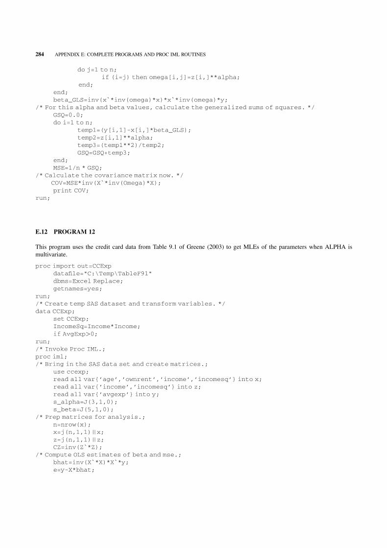
do j=1 to n;
if (i=j) then omega[i,j]=z[i,]**alpha;
end;
end;
beta_GLS=inv(x`*inv(omega)*x)*x`*inv(omega)*y;
/* For this alpha and beta values, calculate the generalized sums of squares. */
GSQ=0.0;
do i=1 to n;
temp1=(y[i,1]-x[i,]*beta_GLS);
temp2=z[i,1]**alpha;
temp3=(temp1**2)/temp2;
GSQ=GSQ+temp3;
end;
MSE=1/n * GSQ;
/* Calculate the covariance matrix now. */
COV=MSE*inv(X`*inv(Omega)*X);
print COV;
run;
E.12 PROGRAM 12
This program uses the credit card data from Table 9.1 of Greene (2003) to get MLEs of the parameters when ALPHA is
multivariate.
proc import out=CCExp
datafile="C:\Temp\TableF91"
dbms=Excel Replace;
getnames=yes;
run;
/* Create temp SAS dataset and transform variables. */
data CCExp;
set CCExp;
IncomeSq=Income*Income;
if AvgExp>0;
run;
/* Invoke Proc IML.;
proc iml;
/* Bring in the SAS data set and create matrices.;
use ccexp;
read all var{’age’,’ownrent’,’income’,’incomesq’} into x;
read all var{’income’,’incomesq’} into z;
read all var{’avgexp’} into y;
s_alpha=J(3,1,0);
s_beta=J(5,1,0);
/* Prep matrices for analysis.;
n=nrow(x);
x=j(n,1,1)||x;
z=j(n,1,1)||z;
CZ=inv(Z`*Z);
/* Compute OLS estimates of beta and mse.;
bhat=inv(X`*X)*X`*y;
e=y-X*bhat;
284 APPENDIX E: COMPLETE PROGRAMS AND PROC IML ROUTINES

/* Log residual square to be used to get alpha values.;
/* Compute alpha values-First iteration.;
r_e=log(e#e);
alpha=inv(z`*z)*z`*r_e;
/* Compute GLS beta values-First iteration.;/
omega=J(n,n,0);
do i=1 to n;
do j=1 to n;
if (i=j) then omega[i,j]=exp(z[i,]*alpha);
end;
end;
beta_GLS=inv(x`*inv(omega)*x)*x`*inv(omega)*y;
/* Update alpha and beta.;
do i=1 to 100;
s_alpha[1,1]=alpha[1,1]; s_alpha[2,1]=alpha[2,1]; s_alpha[3,1]=alpha[3,1];
s_beta[1,1]=beta_GLS[1,1]; s_beta[2,1]=beta_GLS[2,1]; s_beta[3,1]=beta
GLS[3,1];
s_beta[4,1]=beta_GLS[4,1]; s_beta[5,1]=beta_GLS[5,1];
resp=J(n,1,0);
e=y-x*beta_gls;
do j=1 to n;
resp[j,1]=e[j,1]*e[j,1]/exp(z[j,]*alpha) - 1;
end;
alpha=alpha+inv(z`*z)*z`*resp;
/* Get a new value of Beta.;
omega=J(n,n,0);
do i1=1 to n;
do i2=1 to n;
if (i1=i2) then omega[i1,i2]=exp(z[i1,]*alpha);
end;
end;
beta_GLS=inv(x`*inv(omega)*x)*x`*inv(omega)*y;
/* Compute differences.;
diff_beta=sum(abs(s_beta-beta_gls));
diff_alpha=sum(abs(s_alpha-alpha));
diff=diff_beta+diff_alpha;
/* Exit strategy.;
if diff<0.00001 then
do;
print "The estimates of the coefficients are.";
print beta_gls;
print "The value of alpha is " alpha;
print "Convergence was obtained in " i "iterations.";
stop;
end;
end;
var=exp(alpha[1,1]);
var_cov=var*inv(X`*inv(omega)*X);
se=sqrt(vecdiag(var_conv));
STAT_Table=beta_gls||SE;
Print "The estimates of the coefficients are";
Print STAT_Table (|Colname={BHAT SE} rowname={INT Age OwnRent Income
Income2} format=8.4|);
run;
APPENDIX E: COMPLETE PROGRAMS AND PROC IML ROUTINES 285

E.13 PROGRAM 13
This program was used in Chapter 5 to analyze the airlines data found in Table F7.1 of Greene (2003). The code computes the
parameter estimates assuming groupwise heterogeneity.
proc iml;
/* Bring in the SAS data set and create matrices.;
use airline;
read all var{’LnQ’,’LF’,’LnPf’,’D2’,’D3’,’D4’,’D5’,’D6’} into x;
read all var{’D2’,’D3’,’D4’,’D5’,’D6’} into z;
read all var{’LnC’} into y;
s_alpha=J(6,1,0);
s_beta=J(9,1,0);
/* Prep matrices for analysis.;
n=nrow(x);
x=j(n,1,1)||x;
z=j(n,1,1)||z;
CZ=inv(Z`*Z);
/* Compute OLS estimates of beta and mse;
bhat=inv(X`*X)*X`*y;
e=y-X*bhat;
/* Log residual square to be used to get alpha values.;
/* Compute alpha values-First iteration.;
r_e=log(e#e);
alpha=inv(z`*z)*z`*r_e;
/* Compute GLS beta values-First iteration.;
omega=J(n,n,0);
do i=1 to n;
do j=1 to n;
if (i=j) then omega[i,j]=exp(z[i,]*alpha);
end;
end;
beta_GLS=inv(x`*inv(omega)*x)*x`*inv(omega)*y;
/* Update alpha and beta.;
do i=1 to 100;
s_alpha=alpha;
s_beta=beta_GLS;
resp=J(n,1,0);
e=y-x*beta_gls;
sum=J(6,1,0.0);
do j=1 to n;
tem=z[j,]`;
resp[j,1]=e[j,1]*e[j,1]/exp(z[j,]*alpha) - 1;
sum=sum+tem*resp[j,1];
end;
alpha=alpha+inv(z`*z)*sum;
/* Get a new value of Beta.;
omega=J(n,n,0);
do i1=1 to n;
do i2=1 to n;
if (i1=i2) then omega[i1,i2]=exp(z[i1,]*alpha);
end;
end;
beta_GLS=inv(x`*inv(omega)*x)*x`*inv(omega)*y;
286 APPENDIX E: COMPLETE PROGRAMS AND PROC IML ROUTINES

/* Compute differences.;
diff_beta=sum(abs(s_beta-beta_gls));
diff_alpha=sum(abs(s_alpha-alpha));
diff=diff_beta+diff_alpha;
/* Exit strategy.;
if diff<0.00001 then
do;
print "The estimates of the coefficients are.";
print beta_gls;
print "The value of alpha is " alpha;
print "Convergence was obtained in " i "iterations.";
stop;
end;
end;
/* Calculate the covariance matrix at the optimal values.;
omega=J(n,n,0);
do i=1 to n;
do j=1 to n;
if (i=j) then omega[i,j]=exp(z[i,]*alpha);
end;
end;
var_cov=inv(X`*inv(omega)*x);
var_cov_alpha=2*CZ;
se=J(9,1,0);
se_a=J(6,1,0);
do index=1 to 9;
se[index,1]=sqrt(var_cov[index,index]);
end;
do index=1 to 6;
se_a[index,1]=sqrt(var_cov_alpha[index,index]);
end;
print se;
print se_a;
run;
E.14 PROGRAM 14
This program was used in Chapter 7 to estimate the parameters of a dynamic panel data for the cigarettes data set with no
explanatory variables.
* Read the data into SAS;
proc import out=cigar
datafile="C:\Temp\cigar"
dbms=Excel Replace;
getnames=yes;
run;
* Take the Log Transformation;
data cigar;
set cigar;
if state=. or year=. then delete;
Log_C=Log(C);
keep state year Log_C;
APPENDIX E: COMPLETE PROGRAMS AND PROC IML ROUTINES 287

run;
proc iml;
* Define constants;
N=46;T=30;P=406;
* Read the variable into a matrix;
use cigar;
read all var{’Log_C’} into Y;
* H is fixed. So, define H here;
H=shape(0,T-2,T-2);
do j=1 to T-2;
do l=1 to T-2;
if j=l then H[l,j]=2;
if (j=l+1) then H[l,j]=-1;if (j=l-1) then H[l,j]=-1;
end;
end;
* Initialize four sum matrices and the counter;
ZHZ=shape(0,P,P);YMZ=shape(0,1,P);YZ=shape(0,1,P);ZPZ=shape(0,P,P);
compt=1;
do i=1 to N;
* Calculate the diff matrix;
Y_DIFF=shape(0,T-2,1);
Y_DIFFS=shape(0,T-2,1);
do Index=1 to T-2;
Y_DIFF[Index]=Y[Index+compt+1,1]-Y[Index+Compt,1];
Y_DIFFS[Index]=Y[Index+compt,1]-Y[Index+compt-1,1];
end;
* Calculate the BZI matrix;
j=1;cpt=j;cpt2=compt;
BZI=shape(0,1,cpt);BZI[1,1]=Y[cpt2,1];
do j=2 to T-2;
cpt=j;
cpt2=compt;
C=shape(0,1,cpt);
do k=1 to j;
C[1,k]=Y[cpt2+k-1,1];
end;
BZI=block(BZI,C);
end;
* Calculate the matrix sums;
ZHZ=ZHZ+BZI`*H*BZI;
YMZ=YMZ+Y_DIFF`*BZI;
YZ=YZ+Y_DIFFS`*BZI;
compt=compt+T;
end;
* Calculate the first step coefficient estimate;
Delta_Est1=inv(YZ*inv(ZHZ)*YZ`)*YZ*inv(ZHZ)*YMZ`;
print Delta_Est1;
* Calculate the Residual Vector;
compt=1;
do i=1 to N;
* Calculate the diff matrix;
Y_DIFF=shape(0,T-2,1);
Y_DIFFS=shape(0,T-2,1);
E=shape(0,T-2,1);
288 APPENDIX E: COMPLETE PROGRAMS AND PROC IML ROUTINES

do Index=1 to T-2;
Y_DIFF[Index,1]=Y[Index+compt+1,1]-Y[Index+Compt,1];
Y_DIFFS[Index,1]=Y[Index+compt,1]-Y[Index+compt-1,1];
end;
E=Y_DIFF-Delta_Est1*Y_DIFFS;
* Calculate the BZI matrix;
j=1;cpt=j;cpt2=compt;
BZI=shape(0,1,cpt);BZI[1,1]=Y[cpt2,1];
do j=2 to T-2;
cpt=j;cpt2=compt;
C=shape(0,1,cpt);
do k=1 to j;
C[1,k]=Y[cpt2+k-1,1];
end;
BZI=block(BZI,C);
end;
* Calculate the weight matrix for the second step;
ZPZ=ZPZ+BZI`*E*E`*BZI;
compt=compt+T;
end;
* Calculate the second step Arellano and Bond Estimator;
Delta_Est2=inv(YZ*ginv(ZPZ)*YZ`)*YZ*ginv(ZPZ)*YMZ‘;
print Delta_Est2;
run;
E.15 PROGRAM 15
This programwas used inChapter 7 to estimate the cigarettes data set dynamic panelmodelwith explanatory variables. This code
calculates the Anderson–Hso estimator.
* Read the data from Excel;
proc import out=cigar
datafile="C:\Temp\cigar"
dbms=Excel Replace;
getnames=yes;
run;
* Create the log transformations;
data cigar;
set cigar;
if state=. or year=. then delete;
Log_C=Log(C);
Log_MIN=Log(MIN);
Log_NDI=Log(NDI);
Log_Price=Log(Price);
RUN;
proc iml;
* This program will calculate the Anderson-Hso Estimator for the Cigar.TXT dataset;
* Define constants;
N=46;T=30;P=4;
* Read the variables into a matrix;
use cigar;
read all var {’Log_C’,’Log_Min’,’Log_NDI’,’Log_Price’} into Y;
APPENDIX E: COMPLETE PROGRAMS AND PROC IML ROUTINES 289

* Initialize three sum matrices;
ZHZ=shape(0,P,P);YMZ=shape(0,1,P);YZ=shape(0,4,P);
* Initialize the counter;
compt=1;
* Begin the loop for calculating the first step Arellano-Bond Estimator;
do i=1 to N;
* Calculate the diff matrix relating to the Y’s;
Y_DIFF=shape(0,T-2,1);
Y_DIFFS=shape(0,T-2,1);
do Index=1 to T-2;
Y_DIFF[Index,1]=Y[Index+compt+1,1]-Y[Index+Compt,1];
Y_DIFFS[Index,1]=Y[Index+compt,1]-Y[Index+compt-1,1];
end;
* Calculate the diff matrix relating to the X’s;
X_DIFF1=shape(0,T-2,1);
X_DIFF2=shape(0,T-2,1);
X_DIFF3=shape(0,T-2,1);
do index=1 to T-2;
X_DIFF1[Index,1]=Y[Index+compt+1,2]-Y[Index+Compt,2];
X_DIFF2[Index,1]=Y[Index+compt+1,3]-Y[Index+Compt,3];
X_DIFF3[Index,1]=Y[Index+compt+1,4]-Y[Index+Compt,4];
end;
* Create the XI matrix;
XI=shape(0,T-2,4);
XI=Y_DIFFS||X_DIFF1||X_DIFF2||X_DIFF3;
* Calculate the BZI matrix;
BZI=shape(0,t-2,p);
do index=1 to t-2;
BZI[Index,1]=Y[Index+Compt-1,1];
BZI[Index,2]=Y[Index+compt+1,2]-Y[Index+Compt,2];
BZI[Index,3]=Y[Index+compt+1,3]-Y[Index+Compt,3];
BZI[Index,4]=Y[Index+compt+1,4]-Y[Index+Compt,4];
end;
ZHZ=ZHZ+BZI`*BZI;
YMZ=YMZ+Y_DIFF`*BZI;
YZ=YZ+XI`*BZI;
compt=compt+T;
end;
* Calculate the coefficient estimate;
Delta_Est1=inv(YZ*inv(ZHZ)*YZ)*YZ`*inv(ZHZ)*YMZ`;
print Delta_Est1;
run;
E.16 PROGRAM 16
This programwas used inChapter 7 to estimate the cigarettes data set dynamic panelmodelwith explanatory variables. This code
calculates the Arnello–Bond estimator.
proc import out=cigar
datafile="C:\Documents and Settings\E81836\Desktop\Economics Book\cigar"
dbms=Excel Replace;
getnames=yes;
290 APPENDIX E: COMPLETE PROGRAMS AND PROC IML ROUTINES

run;
data cigar;
set cigar;
Log_C=Log(C);
Log_MIN=Log(MIN);
Log_NDI=Log(NDI);
Log_Price=Log(Price);
run;
proc iml;
* This program will calculate the Arellano—Bond estimator for the Cigar.TXT dataset;
* We will assume that all X’s are predetermined;
* Define constants;
N=1;T=30;P=1708;
* Read the variables into a matrix;
use cigar;
read all var {’Log_C’,’Log_Min’,’Log_NDI’,’Log_Price’} into Y;
* H is fixed. So, define H here;
H=shape(0,T-2,T-2);
do j=1 to T-2;
do l=1 to T-2;
if j=l then H[l,j]=2;
if (j=l+1) then H[l,j]=-1;
if (j=l-1) then H[l,j]=-1;
end;
end;
* Initialize Four sum matrices;
ZHZ=shape(0,P,P); YMZ=shape(0,1,P); YZ=shape(0,4,P); ZPZ=shape(0,P,P);
* Initialize the counter;
compt=1;
* Begin the loop for calculating the first step Arellano—Bond estimator;
do i=1 to N;
* Calculate the diff matrix relating to the Y’s;
Y_DIFF=shape(0,T-2,1);
Y_DIFFS=shape(0,T-2,1);
do Index=1 to T-2;
Y_DIFF[Index,1]=Y[Index+compt+1,1]-Y[Index+Compt,1];
Y_DIFFS[Index,1]=Y[Index+compt,1]-Y[Index+compt-1,1];
end;
* Calculate the diff matrix relating to the X’s;
X_DIFF1=shape(0,T-2,1);
X_DIFF2=shape(0,T-2,1);
X_DIFF3=shape(0,T-2,1);
do index=1 to T-2;
X_DIFF1[Index,1]=Y[Index+compt+1,2]-Y[Index+Compt,2];
X_DIFF2[Index,1]=Y[Index+compt+1,3]-Y[Index+Compt,3];
X_DIFF3[Index,1]=Y[Index+compt+1,4]-Y[Index+Compt,4];
end;
* Create the XI matrix;
XI=shape(0,T-2,4);
XI=Y_DIFFS||X_DIFF1||X_DIFF2||X_DIFF3;
* Calculate the BZI matrix;
j=1;
cpt=j+3*(j+1);
APPENDIX E: COMPLETE PROGRAMS AND PROC IML ROUTINES 291

cpt2=compt;
BZI=shape(0,1,cpt);BZI[1,1]=Y[cpt2,1];BZI[1,2]=Y[cpt2,2];
BZI[1,3]=Y[cpt2+1,2];BZI[1,4]=Y[cpt2,3];BZI[1,5]=Y[cpt2+1,3];
BZI[1,6]=Y[cpt2,4];BZI[1,7]=Y[cpt2+1,4];
do j=2 to T-2;
cpt=j+3*(j+1);
cpt2=compt;
C=shape(0,1,cpt);
do k=1 to j;
C[1,k]=Y[cpt2+k-1,1];
end;
do k=1 to j+1;
c[1,j+k]=Y[cpt2+k-1,2];
c[1,j+j+1+k]=Y[cpt2+k-1,3];
c[1,j+2*(j+1)+k]=Y[cpt2+k-1,4];
end;
BZI=block(BZI,C);
end;
ZHZ=ZHZ+BZI`*H*BZI;
YMZ=YMZ+Y_DIFF`*BZI;
YZ=YZ+XI`*BZI;
compt=compt+T;
end;
* Calculate the coefficient estimate;
Delta_Est1=inv(YZ*ginv(ZHZ)*YZ`)*YZ*ginv(ZHZ)*YMZ`;
print Delta_Est1;
* Calculate the Residual Vector;
compt=1;
do i=1 to N;
* Calculate the diff matrix;
Y_DIFF=shape(0,T-2,1);
Y_DIFFS=shape(0,T-2,1);
E=shape(0,T-2,1);
do Index=1 to T-2;
Y_DIFF[Index,1]=Y[Index+compt+1,1]-Y[Index+Compt,1];
Y_DIFFS[Index,1]=Y[Index+compt,1]-Y[Index+compt-1,1];
end;
* Calculate the diff matrix relating to the X’s;
X_DIFF1=shape(0,T-2,1);X_DIFF2=shape(0,T-2,1);X_DIFF3=shape(0,T-2,1);
do index=1 to T-2;
X_DIFF1[Index,1]=Y[Index+compt+1,2]-Y[Index+Compt,2];
X_DIFF2[Index,1]=Y[Index+compt+1,3]-Y[Index+Compt,3];
X_DIFF3[Index,1]=Y[Index+compt+1,4]-Y[Index+Compt,4];
end;
* Create the XI matrix;
XI=shape(0,T-2,4);
XI=Y_DIFFS||X_DIFF1||X_DIFF2||X_DIFF3;
E=Y_DIFF-XI*Delta_Est1;
* Calculate the BZI matrix;
j=1;cpt=j+3*(j+1);cpt2=compt;
BZI=shape(0,1,cpt);BZI[1,1]=Y[cpt2,1];BZI[1,2]=Y[cpt2,2];
BZI[1,3]=Y[cpt2+1,2];BZI[1,4]=Y[cpt2,3];BZI[1,5]=Y[cpt2+1,3];
BZI[1,6]=Y[cpt2,4]; BZI[1,7]=Y[cpt2+1,4];
do j=2 to T-2;
292 APPENDIX E: COMPLETE PROGRAMS AND PROC IML ROUTINES

cpt=j+3*(j+1);
cpt2=compt;
C=shape(0,1,cpt);
do k=1 to j;
C[1,k]=Y[cpt2+k-1,1];
end;
do k=1 to j+1;
c[1,j+k]=Y[cpt2+k-1,2];
c[1,j+j+1+k]=Y[cpt2+k-1,3];
c[1,j+2*(j+1)+k]=Y[cpt2+k-1,4];
end;
BZI=block(BZI,C);
end;
ZPZ=ZPZ+BZI`*E*E`*BZI;
compt=compt+T;
end;
Delta_Est2=inv(YZ*ginv(ZPZ)*YZ`)*YZ*ginv(ZPZ)*YMZ`;
print Delta_Est2;
run;
E.17 PROGRAM 17
This code (including the following comments) was written by Thomas Fomby (Department of Economics, Southern Methodist
University) in 2005. This SAS IMLprogram conducts a duration analysis of the lengths of strikes as a function of the deviation of
output from its trend level, an indicator of the business cycle position of the economy. The data was downloaded from the CD
provided in the Greene textbook, Econometric Analysis, 4th edn., Table A20.1. The data was originally analyzed by J. Kennan
(1985) in his paper “The Duration of Contract Strikes in U.S. Manufacturing,’’ Journal of Econometrics, 28, 55–28.
data strike;
input dur eco;
datalines;
7.00000 .0113800
9.00000 .0113800
13.0000 .0113800
14.0000 .0113800
26.0000 .0113800
29.0000 .0113800
52.0000 .0113800
130.000 .0113800
9.00000 .0229900
37.0000 .0229900
41.0000 .0229900
49.0000 .0229900
52.0000 .0229900
119.000 .0229900
3.00000 -.0395700
17.0000 -.0395700
19.0000 -.0395700
28.0000 -.0395700
72.0000 -.0395700
99.0000 -.0395700
104.000 -.0395700
APPENDIX E: COMPLETE PROGRAMS AND PROC IML ROUTINES 293

114.000 -.0395700
152.000 -.0395700
153.000 -.0395700
216.000 -.0395700
15.0000 -.0546700
61.0000 -.0546700
98.0000 -.0546700
2.00000 .00535000
25.0000 .00535000
85.0000 .00535000
3.00000 .0742700
10.0000 .0742700
1.00000 .0645000
2.00000 .0645000
3.00000 .0645000
3.00000 .0645000
3.00000 .0645000
4.00000 .0645000
8.00000 .0645000
11.0000 .0645000
22.0000 .0645000
23.0000 .0645000
27.0000 .0645000
32.0000 .0645000
33.0000 .0645000
35.0000 .0645000
43.0000 .0645000
43.0000 .0645000
44.0000 .0645000
100.000 .0645000
5.00000 -.104430
49.0000 -.104430
2.00000 -.00700000
12.0000 -.00700000
12.0000 -.00700000
21.0000 -.00700000
21.0000 -.00700000
27.0000 -.00700000
38.0000 -.00700000
42.0000 -.00700000
117.000 -.00700000
;
data strike;
set strike;
dum = 1;
proc iml;
start mle;
use strike;
read all into t var{dur};
read all into x var{eco};
read all into d var{dum};
/* Calculation of Unrestricted MLE estimates using Newton-Raphson Method */
294 APPENDIX E: COMPLETE PROGRAMS AND PROC IML ROUTINES

theta= {1,4,-9};
crit =1;
n=nrow(t);
ones = j(n,1,1);
result=j(10,9,0);
do iter=1 to 10 while (crit>1.0e-10);
sigma=theta[1,1];
beta1=theta[2,1];
beta2=theta[3,1];
w = (ones/sigma)#(log(t) - ones#beta1 - x#beta2);
lnL = d#(w - log(sigma))- exp(w);
lnL = sum(lnL);
g1 = (ones/sigma)#(w#exp(w) - d#(w + ones));
g2=(ones/sigma)#(exp(w) - d);
g3 = (ones/sigma)#x#((exp(w) - d));
g1=sum(g1);
g2=sum(g2);
g3=sum(g3);
g=g1//g2//g3;
h11= -(ones/sigma**2)#((w##2)#exp(w) + 2#w#exp(w) - 2#w#d - d);
h11= sum(h11);
h12= -(ones/sigma**2)#(exp(w) - d + w#exp(w));
h12 = sum(h12);
h13= -(ones/sigma**2)#x#(exp(w) - d + w#exp(w));
h13 = sum(h13);
h21 = h12;
h31 = h13;
h22 = -(ones/sigma**2)#exp(w);
h22 = sum(h22);
h23 = -(ones/sigma**2)#x#exp(w);
h23 = sum(h23);
h32 = h23;
h33 = -(ones/sigma**2)#(x##2)#exp(w);
h33 = sum(h33);
h=(h11||h12||h13)//(h21||h22||h23)//(h31||h32||h33);
db=-inv(h)*g;
thetanew = theta + db;
crit = sqrt(ssq(thetanew-theta));
theta=thetanew;
result[iter,] = iter||(theta‘)||g1||g2||g3||crit||lnL;
end;
lnLu = lnL;
cnames = {iter,sigma,beta1,beta2,g1,g2,g3,crit,lnLu};
print "Calculation of Unrestricted MLE estimates using Hessian-Based Newton-Raphson
Method";
print "Iteration steps ", result[colname=cnames];
print , "Unrestricted Log-likelihood = ", lnLu;
/*Covariance matrix from Hessian*/
cov = -inv(h);
se_sigma_h = sqrt(cov[1,1]);
se_beta1_h = sqrt(cov[2,2]);
se_beta2_h = sqrt(cov[3,3]);
z_sigma_h = sigma/se_sigma_h;
APPENDIX E: COMPLETE PROGRAMS AND PROC IML ROUTINES 295

z_beta1_h = beta1/se_beta1_h;
z_beta2_h = beta2/se_beta2_h;
/*Covariance matrix from BHHH*/
g1 = (ones/sigma)#(w#exp(w) - d#(w + ones));
g2=(ones/sigma)#(exp(w) - d);
g3 = (ones/sigma)#x#((exp(w) - d));
gmat = g1||g2||g3;
bhhh = gmat‘*gmat;
covbh3 = inv(bhhh);
se_sigma_b=sqrt(covbh3[1,1]);
se_beta1_b=sqrt(covbh3[2,2]);
se_beta2_b=sqrt(covbh3[3,3]);
z_sigma_b = sigma/se_sigma_b;
z_beta1_b = beta1/se_beta1_b;
z_beta2_b = beta2/se_beta2_b;
pnames = {sigma,beta1, beta2};
print , "The Maximum Likelihood Estimates: Hessian-Based Newton-Raphson Iteration",
theta [rowname=pnames];
print , "Asymptotic Covariance Matrix-From Hessian", cov
[rowname=pnames colname=pnames];
print "Standard errors: ",se_sigma_h,se_beta1_h,se_beta2_h;
print ,"Asymptotic Covariance Matrix-From bhhh", covbh3
[rowname=pnames colname=pnames];
print "Standard errors: ",se_sigma_b,se_beta1_b, se_beta2_b;
print "Wald test of hypothesis of constant hazard (sigma=1)";
Wald = (sigma-1)*inv(cov[2,2])*(sigma-1); * Wald test;
critval = cinv(.95,1); * calculates the 95th percentile of chi-square 1;
pval = 1 - probchi(wald,1); * calculates the probability value of Wald;
print "Results of Wald test Using Hessian" Wald critval pval;
Wald = (sigma-1)*inv(covbh3[2,2])*(sigma-1); * Wald test;
critval = cinv(.95,1); * calculates the 95th percentile of chi-square 1;
pval = 1 - probchi(wald,1); * calculates the probability value of Wald;
print "Results of Wald test Using BHHH" Wald critval pval;
/* ML Estimation of Restricted Model*/
print , "Maximum Likelihood Estimation of Restricted Model";
print "*************************************************";
theta = {4,-9};
crit = 1;
n = nrow(t);
result = j(10,7,0);
do iter = 1 to 10 while (crit > 1.0e-10);
beta1=theta[1,1];
beta2=theta[2,1];
w = (log(t) - ones#beta1 - x#beta2);
lnLr = d#w - exp(w);
lnLr = sum(lnLr);
g1 = -(d - exp(w));
g1 = sum(g1);
g2 = -x#(d - exp(w));
g2 = sum(g2);
g = g1//g2;
h11 = -exp(w);
296 APPENDIX E: COMPLETE PROGRAMS AND PROC IML ROUTINES

h12 = -x#exp(w);
h22 = -(x##2)#exp(w);
h11 = sum(h11);
h12 = sum(h12);
h21 = h12;
h22 = sum(h22);
h = (h11||h12)//(h21||h22);
db = -inv(h)*g;
thetanew = theta + db;
crit = sqrt(ssq(thetanew - theta));
result[iter,] = iter||(theta‘)||g1||g2||crit||lnLr;
theta = thetanew;
end;
cov = -inv(h);
cnames = {iter,beta1,beta2,g1,g2,crit,lnLr};
print "Iteration steps",result [colname=cnames];
pnames = {beta1,beta2};
print , "The Maximum Likelihood Estimates-Restricted Model", (theta‘)
[colname=pnames];
print , "Asymptotic Covariance Matrix-From Hessian of Restricted Model", cov
[rowname=pnames colname=pnames];
/* Gradient evaluated at restricted MLE estimates */
sigma = 1;
w = (ones/sigma)#(log(t) - ones#beta1 - x#beta2);
g1 = (ones/sigma)#(w#exp(w) - d#(w + ones));
g2=(ones/sigma)#(exp(w) - d);
g3 = (ones/sigma)#x#((exp(w) - d));
gmat = g1||g2||g3;
g1=sum(g1);
g2=sum(g2);
g3=sum(g3);
g=g1//g2//g3;
/* Hessian evaluated at restricted MLE estimates */
h11= -(ones/sigma**2)#((w##2)#exp(w) + 2#w#exp(w) - 2#w#d - d);
h11= sum(h11);
h12= -(ones/sigma**2)#(exp(w) - d + w#exp(w));
h12 = sum(h12);
h13= -(ones/sigma**2)#x#(exp(w) - d + w#exp(w));
h13 = sum(h13);
h21 = h12;
h31 = h13;
h22 = -(ones/sigma**2)#exp(w);
h22 = sum(h22);
h23 = -(ones/sigma**2)#x#exp(w);
h23 = sum(h23);
h32 = h23;
h33 = -(ones/sigma**2)#(x##2)#exp(w);
h33 = sum(h33);
h=(h11||h12||h13)//(h21||h22||h23)//(h31||h32||h33);
LM = g‘*(-inv(h))*g; * LM test;
critval = cinv(.95,1);
pval = 1 - probchi(LM,1);
print "Results of LM test Using Hessian" LM critval pval;
APPENDIX E: COMPLETE PROGRAMS AND PROC IML ROUTINES 297

/* BHHH evaluated at Restricted MLE*/
bhhh = gmat‘*gmat;
covbh3r = inv(bhhh);
LM = g‘*covbh3r*g; * LM test;
critval = cinv(.95,1);
pval = 1 - probchi(LM,1);
print "Results of LM test Using BHHH" LM critval pval;
LR = -2*(lnLr-lnLu); * Likelihood Ratio test;
pval = 1 - probchi(LR,1);
print "Results of LR test" LR critval pval;
/* Let’s see if we get essentially the same maximum likelihood estimates if we use
a BHHH-based Newton-Raphson iteration. */
theta= {1,3.77,-9.35};
crit =1;
n=nrow(t);
ones = j(n,1,1);
result=j(60,9,0);
do iter= 1 to 60 while (crit>1.0e-10);
sigma=theta[1,1];
beta1=theta[2,1];
beta2=theta[3,1];
w = (ones/sigma)#(log(t) - ones#beta1 - x#beta2);
lnL = d#(w - log(sigma))- exp(w);
lnL = sum(lnL);
g1 = (ones/sigma)#(w#exp(w) - d#(w + ones));
g2=(ones/sigma)#(exp(w) - d);
g3 = (ones/sigma)#x#((exp(w) - d));
gmat = g1||g2||g3;
g1 = sum(g1);
g2 = sum(g2);
g3 = sum(g3);
g = g1//g2//g3;
bhhh = gmat‘*gmat;
db= inv(bhhh)*g;
thetanew = theta + db;
crit = sqrt(ssq(thetanew-theta));
theta = thetanew;
result[iter,] = iter||(theta‘)||g1||g2||g3||crit||lnL;
end;
cnames = {iter,sigma,beta1,beta2,g1,g2,g3,crit,lnL};
print "Calculation of Unrestricted MLE estimates using BHHH-Based Newton-Raphson Method";
print "Iteration steps ", result[colname=cnames];
finish;
run mle;
298 APPENDIX E: COMPLETE PROGRAMS AND PROC IML ROUTINES

REFERENCES
Agresti, A. (1990). Categorical Data Analysis, John Wiley & Sons, Inc., New York.
Aigner, D. K. Lovell, and Schmidt, P. (1977). Formulation and Estimation of Stochastic Frontier ProductionModels. Journal of Econometrics,
6: 21–37.
Allison, P. D. (1995). Survival Analysis Using SAS: A Practical Guide, SAS Institute, Inc., Cary, N.C.
Allison, P. D. (2003). Logistic Regression using the SAS� System: Theory and Application, SAS Institute Inc., Cary, NC.
Anderson, T., and Hsiao, C. (1981). Estimation of Dynamic Models with Error Components. Journal of American Statistical Association, 76:
598–606.
Anderson, T., Hsiao, C. (1982). Formulation and Estimation of Dynamic Models Using Panel Data. Journal of Econometrics, 18: 67–82.
Arellano, M. (1987). Computing Robust Standard Errors for Within-Groups Estimators. Oxford Bulletin of Economics and Statistics, 49:
431–434.
Arellano, M., and Bond, S. (1991). Some Tests for Specification for Panel Data: Monte Carlo Evidence and an Application to Employment
Equations. Review of Economic Studies, 58: 277–297.
Ashenfelter, O., Levine, P. B., and Zimmerman, D. J. (2003). Statistics and Econometrics: Methods and Applications, JohnWiley& Sons, Inc.,
New York.
Baltagi, B. H. (2005). Econometric Analysis of Panel Data, John Wiley & Sons, Inc., New York.
Baltagi, B. H. (2008). Econometrics, Springer, New York.
Balatgi, B. H., and Levin, D. (1992). Cigarette taxation: Raising revenues and reducing consumption, Structural Change and Economic
Dynamics 3: 321–335.
Bollerslev, T. (1986). Generalized Autoregressive Conditional Heteroscedasticity. Journal of Econometrics, 31: 307–327.
Breusch, T., and Pagan, A. (1979). A Simple Test for Heteroscedasticity and Random Coefficients Variation. Econometrica, 47: 1287–1294.
Breusch, T., and Pagan, A. (1980). The LM Test and Its Application to Model Specification in Econometrics. Review of Economic Studies, 47:
239–254.
Brocklebank, J. C., and Dickey, D. A. (2003). SAS� for Forecasting Time Series, SAS Institute Inc., Cary, NC.
Brown, B., Durbin, J., and Evans, J. (1975). Techniques for Testing the Constancy of Regression Relationships Over Time. Journal of Royal
Statistical Society, Series B, 37: 149–172.
Casella, G., and Berger, R. L. (1990). Statistical Inference, Wadsworth, Inc., California.
Chow, G. (1960). Tests of Equality Between Sets of Coefficients in Two Linear Regressions. Econometrica, 28: 591–605.
Chung, C. F., Schmidt, P. and Witte, A. D. (1991). Survival Analysis: A Survey, Journal of Quantitative Criminology 7: 59–98.
299
Applied Econometrics Using the SAS� System, by Vivek B. AjmaniCopyright � 2009 John Wiley & Sons, Inc.
Cincera, M. (1997). Patents, R&D, and Technological Spillovers at the Firm Level: Some Evidence from Econometric Count Models
for Panel Data, Journal of Applied Econometrics, 12: 265–280.
Cornwell, C., and Rupert, P. (1988). Efficient Estimation with Panel Data: An Empirical Comparison of Instrumental Variables Estimators.
Journal of Applied Econometrics, 3: 149–155.
Davidson, R., and MacKinnon, J. (1993). Estimation and Inference in Econometrics, New York: Oxford University Press.
Efron, B., and Tibshirani, R. J. (1993). An Introduction to Bootstrap, Chapman & Hall, London, UK.
Enders, W. (2004). Applied Econometric Time Series. John Wiley & Sons, Inc., New York.
Engle, R. (1982). Autoregressive Conditional Heteroscedasticity with Estimates of the Variance of United Kingdom Inflations. Econometrica,
50: 987–1008.
Fomby, T. B. (2007). Department of Economics, Southern Methodist University, Dallas, TX, personal communication, March 31, 2007.
Freund, R., and Littell, R. C. (2000). SAS� System for Regression, 3rd Edition, SAS Institute Inc., Cary, NC.
Freund, R. J., and Wilson, W. J. (1998). Regression Analysis, San Diego, Academic Press.
Fuller, W. A., and Battese, G. E. (1974). Estimation of Linear Models with Crossed-Error Structure. Journal of Econometrics, 2: 67–78.
Glewwe, P. (2006). Department of Applied Economics, St. Paul, MN, personal communication, January 31, 2006.
Graybill, F. A. (2000). Theory and Application of Linear Models, Duxbury Press.
Greene, W. (1992). A Statistical Model for Credit Scoring. Working Paper No. EC-92-29, New York University, Department of Economics,
Stern School of Business.
Greene, W. H. (2003). Econometric Analysis, Prentice Hall, New Jersey.
Grunfeld, Y. (1958). The Determinants of Corporate Investment. Unpublished Ph.D. thesis, Department of Economics, University of Chicago.
Hallam, A. Unpublished Lecture Notes, Department of Economics, Iowa State University, Ames, Iowa.
Hausman, J. (1978). Specification Tests in Econometrics. Econometrica, 46: 1251–1271.
Hausman, J., and Taylor, W. (1977). Panel Data and Unobservable Individual Effects. Econometrica, 45: 919–938.
Hausman, J., and Taylor W. (1981). Panel Data and Unobservable Individual Effects. Econometrica, 49: 1377–1398.
Heckman, J. (1979). Sample Selection Bias as a Specification Error. Econometrica, 47: 153–161.
Hildebrand, G., and T. Liu (1957). Manufacturing Production Functions in the United States. Ithaca, N.Y.: Cornell University Press.
Financial Dictionary, www.investopedia.com, A Forbes Digital Company, 2008.
Jackson, E. J., A User’s Guide to Principal Components, John Wiley & Sons, NY, 2003.
Jaeger, D. A. (2007). Department of Economics, University of Bonn, Germany, April 30, 2007.
Kiviet, J. (1995). On Bias, Inconsistency, and Efficiency of Some Estimators in Dynamic Panel Data Models. Journal of Econometrics,
68(1): 63–78.
Kennan, J. (1985). The Duration of Contract Strikes in U.S. Manufacturing, Journal of Econometrics, 28: 5–28.
Koenker, R. (1981). A Note on Studentizing a Test for Heteroscedasticity. Journal of Econometrics, 17: 107–112.
Koenker, R., and Bassett, G. (1982). Robust Tests for Heteroscedasticity Based on Regression Quantiles. Econometrica, 50: 43–61.
Lee, E. T. (1992). Statistical Methods for Survival Data Analysis, John Wiley & Sons, Inc., New York.
Littell, R. C., Stroup, W. W., and Freund, R. (2002). SAS� for Linear Models, SAS Institute Inc., Cary, NC.
Littell, R. C., Milliken, G. A., Stroup, W. W., and Wolfinger, R. D. (2006). SAS for Mixed Model, 2nd Edition, SAS Institute Inc., Cary, NC.
Lovell, M. C. (2006). A Simple Proof of the FWL (Frisch–Waugh–Lovell) Theorem. Available at SSRN: http://ssrn.com/abstract=887345.
MacKinnon, J., and White, H. (1985). Some Heteroscedasticity Consistent Covariance Matrix Estimators with Improved Finite Sample
Properties. Journal of Econometrics, 19: 305–325.
McCall, B. P. (1995). The Impact of Unemployment Insurance Benefit Levels on Recipiency, Journal of Business and Economic Statistics,
13: 189–198.
McCullough, G. (2005). Department of Applied Economics, St. Paul, MN, personal communication, September 30, 2005.
McLeod,A., and Li,W. (1983). Diagnostic CheckingARMATime SeriesModelsUsing SquaredResidual Correlations. Journal of Time Series
Analysis 4: 269–273.
Meyers, H. M. (1990). Classical and Modern Regression with Applications, PWS-Kent, Massachusetts.
Montgomery, D. C. (1991). Introduction to Statistical Quality Control, John Wiley & Sons, New York.
Mroz, T. (1987). The Sensitivity of an Empirical Model of Married Women�s Hours of Work to Economic and Statistical Assumptions.
Econometrica, 55: 765–799.
Nickell, S. (1981). Biases in Dynamic Models with Fixed Effects. Econometrica, 49: 1417–1426.
NIST/SEMATECH, e-Handbook of Statistical Methods, available at http://www.itl.nist.gov/div898/handbook.
Page, E. S. (1954). Continuous Inspection Schemes. Biometrika, 41(1): 100–115.
300 REFERENCES

Park, H.M. (2005). Linear RegressionModels for Panel Data Using SAS, Stata, LIMDEP and SPSS. TechnicalWorking Paper. The University
Information Technology Services (UITS) Center for Statistics and Mathematics, Indiana University, Indiana.
Sargan, J. D. (1958). The Estimation of Economic Relationships Using Instrumental Variables. Econometrica, 26: 393–415.
Searle, S. R. (1982). Matrix Algebra Useful for Statistics, John Wiley & Sons, Inc., New York.
Snedecor, G. W., and Cochran, W. G. (1983). Statistical Methods, Iowa State University Press, Iowa.
Stokes, M. E., Davis, C. S., and Koch, G. G. (2001). Categorical Data Using the SAS� System, SAS Institute Inc., Cary, NC.
Verbeek, M. (2006). A Guide to Modern Econometrics, John Wiley & Sons Ltd., West Sussex, England.
Walter, E. (2004). Applied Econometric Time Series, John Wiley & Sons, Inc., New York.
White, H. (1980). A Heteroscedasticity-Consistent Covariance Matrix Estimator and a Direct Test for Heteroscedasticity. Econometrica, 48:
817–838.
Woodall, W. H., and Ncube, M. M. (1985). Multivariate CUSUM Quality Control Procedures. Technometrics, 27(3): 285–292.
Wooldridge, J. M. (2002). Econometric Analysis of Cross Section and Panel Data, Massachusetts Institute of Technology, Cambridge, MA.
Zellner, A. (1962).AnEfficientMethod ofEstimating SeeminglyUnrelatedRegression andTests ofAggregationBias. Journal of the American
Statistical Association, 57: 500–509.
REFERENCES 301

INDEX
Accelerated failure time models, 188
Adjusted coefficient of determination, 10
calculation, 10
Adjusted coefficient of variation, 7
definition, 7
Airlines data, 112, 115, 117, 119, 121, 122, 124, 126,
127, 128, 206
fixed/random effects model, covariance matrices, 128
fixed time effects analysis, 121
using Proc GLM, 122
firm effects analysis, 124
using Proc GLM, 126
groupwise heteroscedasticity estimators, 209
HCCME estimators, 220
least squares residuals, 206
comparison, 207
likelihood ratio test, 206
LSDVestimation
using Proc GLM, 119
using Proc IML, 115
using Proc panel, 117
using OLS calculations, 117
mean of residuals, 127
pooled regression model, 112
summary statistics, 254
temporary SAS data set, 208
time series plot, 206
regression, dummy variables, 48
Analysis of variance (ANOVA) techniques, 2, 5, 6, 12, 13, 45, 58
table, 12, 13, 58
ARCH(1) model, 88
process, 89, 91
ARCH(q) process, 89
unconditional variance, 89
Arellano–Bond GMM estimator, 224
first-step estimator, 222
second-step estimator, 222
Asymptotic covariance matrix, 65, 114, 234
Asymptotic variance, 116
Asymptotic variance-covariance matrix, 57
Attrition models, 153
Autocorrelation process, 93–96
detection, 96–101
Durbin–Watson test, 96
Lagrange multiplier test, 97
first-order, 96
occurrence, 93
ordinary least square (OLS) estimation problems,
94–95
parameters, 101, 102
FGLS estimation method, 101
GLS estimation method, 101
second-order, 96, 102, 104
Autoregressive conditional heteroscedastic models (ARCH)
44, 87–92
generalized ARCH models, 44, 89
process, 88, 91
testing effects, 90–92
Autoregressive autocorrelation model (AR) 101–109
AR(2) model, residuals, 102–105, 108, 109
first-order autocorrelation model (AR1) 94
fitness procedure, 101
Proc autoreg, 101
SAS usage, 101
Autoregressive moving average process, 88
Bartlett test statistic, 207
variance comparison, 207
Applied Econometrics Using the SAS� System, by Vivek B. AjmaniCopyright � 2009 John Wiley & Sons, Inc.
303

BHHH methods, algorithm, 192
Binary response models, 154
Bootstrap estimation method, 262, 267
calculating standard errors, 264
cumulative distributions, plot diagram, 263
estimation technique, 262
in regression analysis, 265
in SAS, 264
lower/upper confidence limit, 263
OLS estimates, 271
Proc Univariate statements, 265
Bootstrapped regression analysis, 267–269
gasoline consumption data, 269
residuals method, 266, 268
SAS, 267
Breusch–Pagan Lagrange multiplier test, 76, 78–80, 129
credit card expenditure data, 80
Central limit theorem, 5
Ceteris paribus condition, 2
Chi-square test, 191
distribution, 97, 207
table, 66
values, 189
Chow test static, 40, 41, 42
by Proc model, 42
structural break in gasoline data, 42–43
p value, 40, 41
Classical regression model, spherical disturbances assumption, 71
Cobb–Douglas model, 34, 35, 37
production data, 35
regression analysis, 35, 37
SAS code, 35
Coefficient of determination, 10, 14
calculation, 10
Coefficient of variation, 13, 51
definition, 13
Combined gasoline consumption data,
regression analysis, 41
Complex panel data models, 116
autocorrelation violations, 116
dynamic panel data models, 116
heteroscedasticity violations, 116
Conditional probabilities, 173
calculation, 173
Confidence interval, 7–8, 18, 189
Consumer price index (CPI), 9, 14
inflation rate, 14
Cook’s D statistic, definition, 20
Cook’s statistic, See Cook’s D statistic
Correlation, 15, 16
b/w variables, 16
coefficients, 25
matrix, 26
nature of, 15
scatter plots, 15
Covariance matrix, 95, 125, 128
construction, 95
diagonal elements, 125
Cox’s proportional hazard models, 190
CPI, See Consumer price index
Credit card expenditure data, 203
ALPHA vs. likelihood value plot, 281
Breusch–Pagan Lagrange multiplier test, 279
FGLS estimators, 280
GLS estimator, 283
heteroscedasticity, 278
iterative FGLS estimators, 203
maximum likelihood estimations (MLEs) parameters, 284
regression analysis, 205
White’s test, 278
Cross-equation correlation, 1, 140
Cross-model covariance matrix, 140
diagonal elements of, 140
Cumulative distribution function (CDF), 170
Cumulative hazard rate function, 171
CUSUM test, 41–45
critical values, 43
definition, 43
gasoline consumption data, 44, 45
plot, 45
procedure, 41
Data matrix, 7, 10
Data plotting, 15–16
Data set, 47
Data testing, 38
for structural breaks, 38
linear restriction hypothesis test, 38
Davidson/MacKinnon’s estimator, 81
DM1versions, 83
DM2 versions, 83
Definite matrix, 53
Degrees of freedom, 6, 13, 29, 65, 91
model, 10, 50
n–k, 29
Dependent variable, 6, 18
predictions of, 18–21
Determinants, 241
definition, 241
properties of, 241
Direct marketing companies, 153
Discrete choice models, 153
binary response models, 154
parameters interpretation, 155
shortcomings, 154
Discrete random variable, 153
Disturbance vector, 114
Dummy variables, 45
estimators, 72, 113
in models, 45–51
model, 114
vector, 114
Duration analysis, 169, 178
distribution functions, 178–186
exponential distribution, 179
lognormal distribution, 184
Weibull distribution, 179
304 INDEX

Durbin–Watson statistic test, 91, 96, 97, 101, 102
Box and Pierce’s test (B&P), 97
error sums of squares, 90
Ljung’s modification, 97
mean sums of squares, 90
serial correlation, 90
Dynamic panel data models, 220
dynamic panel data estimation, 221
generalized methods of moments
estimation (GMM), 220
estimation technique, 221
with explanatory variables, 223
Earning’s equation model, 47
data matrix, 47
dummy variable, 47
Elasticity, 2
definition, 2
vs. marginal effect, 2
Endogeneity, alternative hypothesis, 64
Engle’s ARCH model, See ARCH(1) model
Error sums of squares (SSE), 4, 78
Explanatory variables, 2, 3, 24, 45, 54, 55, 70, 71, 75, 110, 111,
114, 118, 129
categories, 45
estimation, 71
feasible generalized least squares (FGLS)
estimators, 71
generalized least squares (GLS)
estimators, 71
measurement errors, 54, 55
revisited estimation, 80
types, 110
observed/controllable, 110
unobserved/uncontrollable, 110
Exponential distribution, 179, 183
hazard function, 179, 183
probability density function, 179
survival function, 179, 183
Extra variable model, 7
sums of squares of error, 7
F-statistic value, 13, 25, 30, 64, 121
formula, 29, 34, 37, 39
critical value, 37
Proc IML use, 29
hypothesis tests, 13
Failure times/censoring, 169–170
Feasible generalized least squares (FGLS),
134
asymptotic covariance matrix, 134
cross-equation covariance, 140
estimation, 84, 87, 88
by credit card data, 87, 88
estimator, 86, 102, 232
cross-sectional correlation, 232
general procedure, 86
Proc Reg output, 86
SAS step, 86
standard errors, 233
Grunfeld’s investment data set, 134, 135
OLS residuals, 134
Fitted/full model, 93
degree of autocorrelation, 93
residuals, 93
Fixed effects model, 113–123
estimation methods, 113
between-group effects approach, 113
least squares dummy variable approach, 113
within-group effects approach, 113
Proc GLM, 118
Frisch–Waugh theorem, 6, 114
GARCH model, 89–91
effects, 91
principle, 90
unconditional variance, 90
Gasoline consumption data, 38, 94, 98, 99, 100, 101,
103, 104, 105, 107, 108, 109
AR(1) model, 100
iterated FGLS estimates, 107
output, 100, 101
AR(2) model, 101, 104, 105
iterated FGLS estimates, 108
MLE estimates, 103, 105
output, 101
AR models, residuals comparison, 109
autocorrelation, 98, 99
Durbin–Watson statistics, 98
Proc Autoreg detecting method, 98, 99
full model residuals, 94
time series plot, 94
independent variables, 26
Proc Corr output, 26
model, 93
multicollinearity output, 25
OLS vs. AR(2) models, 109
residuals comparison, 109
reduced model residuals, 94
time series plot, 94
regression analysis, 39, 40
Gauss–Markov theorem, 5
Generalized least squares (GLS) estimation technique,
86, 133
estimator, 96
Generalized methods of moments estimation (GMM), 148, 220
Arellano–Bond, 224
cigar.txt panel data, 222
dynamic panel data models, 220, 221
estimators, 150
2SLS, 151
labor equation, 150
weight matrix, 151
White’s estimator, 151
explanatory variables, 223
optimal weight matrix, 221
INDEX 305

General linear hypothesis, 27, 28, 29
hypothetical model, 27
least squares estimator, 28
restriction equation, 27
SAS use, 29
testing, 33
Proc Reg output, 34
variance-covariance matrix, 28
General panel data model, 111, 120
GNP, See Gross national product
Goldfeld–Quandt tests, 78
explanatory variable, 78
Good fit model, 25
Goodness-of-fit statistics, 6–7, 185
adjusted coefficient of determination, 6
assessment method, 185
Proc Lifereg, 185
coefficient of determination, 6
definition, 6
Gross national product, 9
Group-specific mean square errors, 207
Groupwise heteroscedasticity estimator, 205, 209
airlines data analysis, 205
airlines data set, 208, 209
assumption for model, 208
Chi-squared distribution, 207
homoscedasticity assumption, 205
likelihood ratio test, 206
mean square error (MSE), 207
using Harvey’s multiplicative heteroscedasticity approach, 210
Grunfeld data analysis, 136
using Proc Syslin SUR, 136–140
Grunfeld data set, 134, 135, 228
FGLS estimator, 229
FGLS pooled estimators, 228
pooled OLS regression, 135
Proc Syslin SUR, 136
Grunfeld investment model, 1
Harvey’s multiplicative heteroscedasticity, 204, 208
MLE estimates, 204
single parameter, 204
model parameters estimation, 204
variance-covariance matrix, 205
Hausman analysis, 65
by Proc IML, 65
consumption data, 65
Hausman’s specification test, 61, 64–69, 128–130
by Proc model, 66–69
consumption data, 66
generation, 129
Hausman–Taylor estimator, 210
coefficients estimates, 212
endogenous/exogenous variables, 210
for random effects model, 210
instrumental variables, 212
Proc IML, 218
Proc model output, 216–217
PSID, 212
random effects and LSDV model, 212
standard errors, 218
steps, 211
wages equation, 219
Hazard function, 170–178
definition, 170
HCCME estimators, 82
credit card data, 82
OLS estimate of covariance matrix, 219
Heteroscedasticity, 70, 71, 72, 74, 76, 78, 91
detection, 72, 74
formal hypothesis tests, 74–80
least squares residuals, 72
residual plots, 78
testing, 91
nominal exchange data, 91
variance-covariance matrix, 71
Heteroscedastic variance, 22
funnel-shaped graph, 22
Homoscedasticity, 80, 207
null hypothesis, 80, 207
Human’s specification test, 151
exogenous/endogenous variable, 151
OLS/2SLS estimates, 152
Proc model procedure, 151
Hypothesis testing, 7–8, 27, 28, 39
confidence intervals, 8
linear restrictions, 28
regression coefficient, 8
Idempotent matrices, 243
definition, 243
econometrics, 243
Identity matrix, 240
definition, 240
properties, 240
Independent disturbances, 93
assumption, 93
Independent regressions, 78
Independent variables, See Explanatory variables
Inflation rate, 14, 15
definition, 14
Instrumental variables, 52, 55, 56
estimation of, 55–60
covariance matrix, 56
data matrix, 60
standard error, 58, 60
data matrix, 56
least squares model, 55
matrix, 56
exper, 56
exper2, 56
motheduc, 56
regression, 58
Instrumental variables analysis, 58
Proc Syslin, 58
earning data, 58
306 INDEX

Insurance companies, 153
Inverse matrix, 242
construction of, 242
definition, 242
Proc IML, 243
properties of, 242
Investment equation model, 14, 17
complete data set, 14
correlation analysis, 17
Investment equation regression analysis, 21
Iterative FGLS estimation, 202
credit card expenditure data, 203
estimation process, steps, 203
estimators, 202
heteroscedasticity, 202
Joint distribution, 202
log-likelihood function, 203
maximum likelihood estimation, 202
OLS residuals, 202
two-step estimation process, 202
Kaplan Meier method, 172
survival function, 176
bar graph, 176
Kronecker products, 244
econometric data analysis, 244
FGLS estimation, 244
properties of, 244
Lagrange multiplier test (LM), 79, 90, 97, 129, 192
ARCH(q) effects, 90
steps, 90
Least squares dummy variable (LSDV) model, 113, 114,
116, 118
coefficient of determination, 118
disadvantage, 113
error degrees of freedom, 118
parameter estimation, 116
OLS, 116
root mean square, 118
Least squares estimation method, 1, 4, 55, 96, 125
parameters, 96
FGLS, 96
iterated FGLS, 96
MLE, 96
Least squares estimator, 4, 5, 24, 30, 39, 52, 53, 71, 80, 102
asymptotic normality, 5
consistency, 4
correlation, 24
instrumental variables estimator, 57
probability limits, 52
unrestricted, 39
variance, 24
Least squares theory, 3–5
Linear functions, derivatives, 247
Linear model(s), 2, 6, 53, 70, 71, 89
assumptions, 2
conditional expectation, 53
disturbance vector, 70
symmetric matrix, 71
variance, 70
Linear regression, 72
Linear restriction hypothesis, 28
F statistic, 28
Log-likelihood function, 203
credit card data set plot, 89, 204
values, 89
Log-log model, 2
marginal effect, 2
Lognormal distribution, 184, 185
cumulative density function, 184
hazard functions, 184, 185
bar graph, 185
probability density function, 184
survival functions, 184, 185
bar graph, 185
Marginal effects, 2
Matrix, 237
addition and subtraction operations, 238
definitions, 237
diagonal matrix, 238
identity matrix, 238
multiplication operations, 239
properties of, 245
rank, 245
definition, 245
full rank, 245
properties of, 245
scalar multiplication operations, 238
square matrix, 238
trace,
definition, 241
properties of, 242
transpose of, 240
Matrix algebra, 239, 246
associative laws, 239
commutative laws of addition, 239
differential calculus, 246
Hessian matrix, 246
Jacobian matrix, 246
simple linear function derivatives, 246
distributive laws, 239
Maximum likelihood estimation (MLE), 86, 206
multivariate value, 206
Mean intervals, 20
for investment equation data, 18–19
prediction graphs, 18
Proc Reg output, 20
Mean square error, 13, 28, 207, 211, 268
Model of interest, 46
Mroz2, See Temporary SAS data set
Multicollinearity, 24–26
degree of correlation, 24
p values, 25
sets of statistics, 24
INDEX 307

Multiple linear regression model, 1, 3, 4
matrix form, 3
Newton–Raphson method, 157–163, 192
algorithm, 157
for Logit model, 157–163
Nonspherical disturbances, 70, 71
autocorrelation, 70
heteroscedasticity, 70
Null hypothesis, 6, 8, 13, 29, 30, 32, 61, 62, 65, 80, 101, 128, 129
Off-diagonal elements, 140
Omitted variable model, 53
bias, 53
Ordinary least squares (OLS) analysis, 58, 59, 72, 86, 149
earning data, 59
estimator, 4, 31, 33, 53, 56, 83, 102, 255, 256
consistency, 56
histogram of, 257–260
labor equation, 149
mean and standard deviation, 256
probability, 53
simulated type, 1 error rate, 256
estimation, 58, 82, 234
covariance matrix, 82
critical assumption, 142
equation-by-equation, 140
estimation techniques, 144
keynesian model, 143
problems, 142–144
standard errors, 82
structural equation, 144
model, 58, 97, 104, 154
of credit card expenses data, 72
regression statistics, 25
residuals, 75, 86
Overidentifying restrictions testing, 63
in earning data, 63
Panel data method, 110, 111
advantages, 110–111
definition, 110
overview, 110
Panel data models, 111–112, 219, 224
autocorrelation, 224, 227
covariance matrices, robust estimation of, 219
FGLS methods estimators, 225
fixed effects, 111
GLS estimation, 225
heterogeneity, 224
homoscedastic disturbances, 219
ordinary least squares estimation method, 111
pooled regression, 111
PROC IML code, 226
random effects, 111
Poisson regression, 163–165
estimation, 165–168
parameters interpretation, 165
Pooled regression model, 112–113, 118
coefficient of determination, 113
expression equation, 113
parameters estimation, 112
OLS, 112
root mean square error, 113, 118
Prais–Winsten Method, 234
transformations, 96
usage, 96
Prediction intervals graphs, 21
Proc Reg output, 21
Price index of gasoline (Pg), 38
Probability distribution function, 171
Probability of failure (PDF), 174
calculation, 174
Probability plots, 22
Probit and Logit models, 155
estimation/inference, 156
Proc autoreg, 96, 102
CUSUMLB procedure, 44
CUSUMUB procedure, 44
usage, 102
reference guide, 91
Proc Corr procedure, 16
general form, 16
Proc GLM, 49, 121
airlines data regression, 49–50
data analysis, 49
dummy variables, 49
Proc Gplot, 16, 20
confidence intervals, 20
Proc IML analysis, 11, 47, 57, 114, 204, 248, 272
1�1 matrices, 249
Anderson–estimator, 289
Arellano–Bond method, 224, 290
code computes, 286
concatenate matrices, 252
control statements, 252
CPI, 272
create row and column vectors, 237
creating matrices/vectors operations, 249
data analysis, 47, 57
data matrix, 57
determinants of matrices, 241
diag command, 252
diagonal matrix, 251
DO-END statement, 253
DO iterative statement, 253
dynamic panel data, 287
econometric analysis, 251
elementary matrix operations, 250
addition/subtraction, 250
inverses, eigenvalues, and eigenvectors, 250
Kronecker products, 250
GMM calculations, 222
GNP and Invest time series, 272
groupwise heterogeneity, 286
Grunfeld’s data analysis, 229
308 INDEX

Hausman’s specification test, 212, 276
Hausman–Taylor’s estimates, 218
heteroscedasticity, 277
identity matrix, 240
IF-THEN/ELSE statement, 253
Kronecker products calculation, 244
linear equations, 248
linear hypothesis, 275
matrix-generating functions, 251
block diagonal matrices, 251
diagonal matrix, 251
identity matrix, 251
J matrix, 251
matrix inverses, 243
matrix multiplications, 239
max(min) commands, 251
of investment data, 11
Proc IML code, 273
restricted least squares estimator, 274
robust variance-covariance matrices, 277
SAS procedures, 212
standard errors of estimator, 274
statements, 30
SUMMARY command, 253
trace of a matrix, 242
transpose matrix, 240
VecDiag function, 252
White’s test, 277–278
within-group mean residuals
estimates, 215
Proc IML code, 226
FGLS estimator, 226
general linear hypothesis, 273
Kronecker product, 244
Proc IML command, 65, 237
create row and column vectors, 237
identity matrix, 238
matrix multiplications, 239
trace of a matrix, 241
Proc IML diag command, 252
diagonal matrix, 252
Proc Import statement, 9
Proc Life procedure, 173
Proc Lifereg models, 178, 191
Proc Lifetest analysis, 173, 175, 178
tabular presentation, 175
Proc Lifetime, 177
Proc model, 151, 215
HCCME option, 219
instrumental variable regression, 215
OLS/2SLS models, 151
procedure, 76
Proc Panel, 81, 114, 116–118, 120, 121, 123, 125, 128–131,
212, 219–221
documentation, 81
procedure, 114
Proc Plot procedure, 15
statements for, 15
Proc Reg analysis, 12, 15, 32, 47, 62, 101, 151, 255
data analysis, 47
endogeneity, 62
investment equation data, 15
of investment data, 12
OLS estimates, 32
tableout option of, 255
t test, 32
Proc Reg module, 21
Proc Reg statements, 268
OLS regression, 268
Proc Syslin, 60, 151
earning data output, 60
procedure, 148
Proc Univariate, 255
data, 213
histogram option, 255
module, 22
Production data-translog model, 36
regression analysis, 36
Quadratic form, derivative of, 247
Quarterly investment data, 31, 33
Proc IML output, 31
Proc Reg output, 33
Random effects model, 123–131, 210
estimation, 130–131
Hausman–Taylor estimator, 210
random disturbances, assumptions, 211
tabular presentation, 130
tests, 125–128
Hausman specification, 125
Lagrange multiplier (LM), 125
Wages data, 213
Rank, 245
definition, 245
equivalence, 246
Proc IML, 245
properties of, 245
Real _Invest
scatter plot, 18
vs. time plot, 17
vs. time trend, 18
vs. Real GNP plot, 16
Real_GNP coefficient, 14
RECID data, 172, 173, 175–177, 179, 180, 185, 186, 188, 190, 192
exponential distribution, 188
Kaplan Meier survival function plot, 176
lifetime hazard function plot, 179
lifetime survival function plot, 176, 177
normal distribution fit, 186, 192
Proc Lifetest analysis, 173
survival functions testing, 180–182
Weibull distribution fit, 190
REG procedure model, 12, 15, 18, 25, 33–37, 39–41, 46, 48, 59,
62–64, 72, 85, 87, 88, 112, 135, 149, 160, 186, 188, 190, 192,
194, 195, 201, 205, 209, 214, 269, 270
INDEX 309

Regression analysis, 1, 3, 8, 9, 18, 24, 46, 78, 178, 205
assumptions, 3
objectives, 3, 18
by Proc IML, 9
data analysis, 10
data reading, 9
By Proc Reg, 12, 46
data analysis, 12
data interpretation, 12
earnings data, 46
credit card expenditure data, 205
parameters interpretation, 2
Proc Lifereg, 178
Proc Phreg, 178
residual analysis, 8
Regression coefficient(s), 13, 18
Regression model(s), 1, 14, 53, 61, 93, 187
adjusted R2 value, 14
autocorrelation, 93
coefficient of determination (R2), 14
Cox proportional hazard, 187
dependent variable, 1
endogeneity, 53
endogenous explanatory variable, 61
independent variable, 1
parametric, 187
testing overidentifying restrictions, 61
Regression summary statistics, 79
credit card expenditure data, 79
Residual analysis, 20–23
column, 19
Proc Reg, 20
residual graphs, 21
types of plots, 8
Residual vector, definition, 4, 7
Residuals, 21–23, 73, 92
GARCH model, 92
normal probability plot, 22, 23
standardized, definition, 20
vs. age plot, 73
vs. average expense plot, 73
vs. income plot, 74
vs. predicted response plot, 21
vs. predicted values plot, 23
vs. time plot, 22
Response variable, 170
Response vector, 10
Restricted least squares estimator, 31–33
least squares estimator, 31
Proc IML output, 32
of variance-covariance matrix, 32
standard errors, 32
variance expression, 31
variance-covariance matrix, 31, 32
Restricted model, See Cobb-Douglas model
Robust estimators, 84
Proc IML output, 84
variance-covariance matrix, 84
Root mean square error (RMSE), 19, 78,
87, 268
Sargan’s hypothesis test, 61
regression-based, 61
steps, 61–62
SAS system, 79, 90, 267
bootstrapped regression analysis, 267–271
Breusch–Pagan test, 79
code usage, 120
data set, 9, 10, 65
data step statements, 217
IML program, 293
Log transformations, 267
Proc autoreg module, 90
Proc model statements, 40
program, 220
data simulation, 256
statements, 18, 66, 81, 256
test, 78
Seemingly unrelated regression (SUR) models, 132, 133,
138, 139, 244
equations, 40
GLS estimator, 133
OLS model, 133
system, 58
Semi-log model, 2, 47, 57
earnings model, 47
elasticity, 2
marginal effect, 2
Serial correlation, 95
assumptions estimation, 95
Simple linear regression model, 3, 54, 55
explanatory variable, 54
least squares estimation, 3
testing steps, 61
Simple panel data models, 116
analyzing method, 116
Proc Panel, 116
Proc TSCSREG procedure, 116
Simultaneous equation models, 142
Hausman’s specification test, 151
identification problem, 145
endogenous variables, 147
exogenous variables, 147
structural equation parameters, 144–146
OLS estimation problems, 142–144
OLS regression, 148
Proc Syslin procedure, 148
reduced form equations, 144–145
two-stage least squares (2SLS) method, 147
Wage-price inflation equation, 142
specification tests, 61
explanatory variables, 63
instrumental variables, 63
testing overidentifying restrictions, 61
weak instruments, 63
Spherical disturbances, 70
310 INDEX

Standard error(s), 18, 86, 87
column, 14
definition, 8
Strike data duration analysis, 196–200
Subject-specific heterogeneity, 111, 113, 123
effects, 128, 129
Sums of squares for error (SSE), 5, 7
Sums of squares for regression (SSR), 5
Survival function, 170–178
definition, 170
Kaplan Meier method, 172
life table method, 172
plot, 176
standard error, 172
Temporary SAS data set, 9, 10, 61, 65, 90, 172, 186, 208
Test statistic, 11, 28–30, 65, 66, 78, 79
Proc IML statements, 79
value, 14, 79
Time series data, 93
Translog model, 35, 36
Transpose matrix, 240
definition, 240
properties, 240
True population model, 54
OLS estimate, 54
probability limits, 54
Two-stage least squares estimator (2SLS) analysis, 56, 62, 148
assumption of homoscedastic disturbances, 148
labor equation, 149
weight matrix, 151
Two-way fixed effects model, 123
Proc GLM estimation method, 123
Unbiased estimator, 5, 8, 33, 71, 266
Unknown coefficients, 1, 2
U.S. gasoline consumption (G), 38
time series plot, 38
Variance, 5, 95
Variance-covariance matrix, 95, 113
Variance inflation factors (VIF), 24
values, 25
Wage equation, 56, 64
regression equation, 64
Wages data, 213
random effects model, 213
within-group effects model, 214
Wald’s chi-square test, 161, 192
values, 161, 188
Weak instruments analysis, 64
in earning data, 64
Weibull distribution, 179, 183, 184, 190
cumulative density function, 179
hazard functions, 183
probability density function, 179
survival function, 184
bar graph, 184
Weighted least squares regression
methods, 84, 85
credit card expenditure data, 85
Proc Reg option, 84
SAS statements, 84
White’s estimator, 80, 81, 83, 148, 219, 220
Proc model statements, 81
HCCME option, 81
variance-covariance matrix, 80
White’s general test, 74–78
credit card expense data, 76–78
Proc IML programme, 74
test statistic value, 76
Within-group model, 113, 120, 211, 212
disadvantages, 113
disturbance variances, 207, 208
GLS estimation, 207
merge data, 208
OLS model, 208
time-invariant disturbance, 211
residuals vector, 207, 215
root mean square, 120
Wages data, 214
INDEX 311