SAS/GRAPH and Base SAS 9.4: Mapping Reference
648
SAS/GRAPH ® and Base SAS ® 9.4: Mapping Reference SAS ® Documentation June 8, 2022
-
Upload
khangminh22 -
Category
Documents
-
view
1 -
download
0
Transcript of SAS/GRAPH and Base SAS 9.4: Mapping Reference

SAS/GRAPH® and Base SAS® 9.4: Mapping Reference
SAS® DocumentationJune 8, 2022

The correct bibliographic citation for this manual is as follows: SAS Institute Inc. 2017. SAS/GRAPH® and Base SAS® 9.4: Mapping Reference. Cary, NC: SAS Institute Inc.
SAS/GRAPH® and Base SAS® 9.4: Mapping Reference
Copyright © 2017, SAS Institute Inc., Cary, NC, USA
All Rights Reserved. Produced in the United States of America.
For a hard copy book: No part of this publication may be reproduced, stored in a retrieval system, or transmitted, in any form or by any means, electronic, mechanical, photocopying, or otherwise, without the prior written permission of the publisher, SAS Institute Inc.
For a web download or e-book: Your use of this publication shall be governed by the terms established by the vendor at the time you acquire this publication.
The scanning, uploading, and distribution of this book via the Internet or any other means without the permission of the publisher is illegal and punishable by law. Please purchase only authorized electronic editions and do not participate in or encourage electronic piracy of copyrighted materials. Your support of others' rights is appreciated.
U.S. Government License Rights; Restricted Rights: The Software and its documentation is commercial computer software developed at private expense and is provided with RESTRICTED RIGHTS to the United States Government. Use, duplication, or disclosure of the Software by the United States Government is subject to the license terms of this Agreement pursuant to, as applicable, FAR 12.212, DFAR 227.7202-1(a), DFAR 227.7202-3(a), and DFAR 227.7202-4, and, to the extent required under U.S. federal law, the minimum restricted rights as set out in FAR 52.227-19 (DEC 2007). If FAR 52.227-19 is applicable, this provision serves as notice under clause (c) thereof and no other notice is required to be affixed to the Software or documentation. The Government’s rights in Software and documentation shall be only those set forth in this Agreement.
SAS Institute Inc., SAS Campus Drive, Cary, NC 27513-2414
June 2022
SAS® and all other SAS Institute Inc. product or service names are registered trademarks or trademarks of SAS Institute Inc. in the USA and other countries. ® indicates USA registration.
Other brand and product names are trademarks of their respective companies.
9.4_01-P6:grmapref

Contents
About This Book . . . . . . . . . . . . . . . . . . . . . . . . . . . . . . . . . . . . . . . . . . . . . . . . . . . . . . . . . . viiWhat’s New in SAS/GRAPH and Base SAS 9.4: Mapping Reference . . . . . . . . . . . . . xvii
PART 1 Getting Started 1
Chapter 1 / Get Started Mapping Using SAS/GRAPH and Base SAS . . . . . . . . . . . . . . . . . . . . . . . . . . . 3What Is Mapping Software? . . . . . . . . . . . . . . . . . . . . . . . . . . . . . . . . . . . . . . . . . . . . . . . . 3Components of Base SAS Mapping Software . . . . . . . . . . . . . . . . . . . . . . . . . . . . . . . . . 5Components of SAS/GRAPH Mapping Software . . . . . . . . . . . . . . . . . . . . . . . . . . . . . . 6Maps You Can Create Using Mapping Software . . . . . . . . . . . . . . . . . . . . . . . . . . . . . . 7What You Need to Know to Get Started . . . . . . . . . . . . . . . . . . . . . . . . . . . . . . . . . . . . . . 8Learning By Example: Create Your First Map . . . . . . . . . . . . . . . . . . . . . . . . . . . . . . . . 19Where to Go from Here . . . . . . . . . . . . . . . . . . . . . . . . . . . . . . . . . . . . . . . . . . . . . . . . . . . 24
Chapter 2 / Gallery of Maps . . . . . . . . . . . . . . . . . . . . . . . . . . . . . . . . . . . . . . . . . . . . . . . . . . . . . . . . . . . . . 27A Quick Look at the Gallery . . . . . . . . . . . . . . . . . . . . . . . . . . . . . . . . . . . . . . . . . . . . . . . 27Gallery of Base SAS ODS Graphics and SAS/GRAPH Maps . . . . . . . . . . . . . . . . . . 28Base SAS Procedures to Prepare Map Data . . . . . . . . . . . . . . . . . . . . . . . . . . . . . . . . 32
Chapter 3 / Common Tasks Associated with Developing Mapping Programs . . . . . . . . . . . . . . . . . . 35About the Base SAS and SAS/GRAPH Tasks . . . . . . . . . . . . . . . . . . . . . . . . . . . . . . . 35Output Environment Tasks . . . . . . . . . . . . . . . . . . . . . . . . . . . . . . . . . . . . . . . . . . . . . . . . 36Map Creation Tasks . . . . . . . . . . . . . . . . . . . . . . . . . . . . . . . . . . . . . . . . . . . . . . . . . . . . . . 36Map Enhancement Tasks . . . . . . . . . . . . . . . . . . . . . . . . . . . . . . . . . . . . . . . . . . . . . . . . . 37
Chapter 4 / Additional Resources to Help You Develop Your Mapping Programs . . . . . . . . . . . . . . . 39Base SAS and SAS/GRAPH Sample Programs . . . . . . . . . . . . . . . . . . . . . . . . . . . . . . 39Examples and Resources on the Web . . . . . . . . . . . . . . . . . . . . . . . . . . . . . . . . . . . . . . 42Using Run-Group Processing . . . . . . . . . . . . . . . . . . . . . . . . . . . . . . . . . . . . . . . . . . . . . 43RUN-group Processing with Global and Local Statements . . . . . . . . . . . . . . . . . . . . 43RUN-group Processing with BY Statements . . . . . . . . . . . . . . . . . . . . . . . . . . . . . . . . . 43RUN-group Processing with the WHERE Statement . . . . . . . . . . . . . . . . . . . . . . . . . . 44Books . . . . . . . . . . . . . . . . . . . . . . . . . . . . . . . . . . . . . . . . . . . . . . . . . . . . . . . . . . . . . . . . . . 44
PART 2 Mapping: SAS/GRAPH and Base SAS Statements, System Options, and Macros 45
Chapter 5 / SAS/GRAPH Statements . . . . . . . . . . . . . . . . . . . . . . . . . . . . . . . . . . . . . . . . . . . . . . . . . . . . . 47Overview of Global Statements . . . . . . . . . . . . . . . . . . . . . . . . . . . . . . . . . . . . . . . . . . . . 47

Specifying Units of Measurement . . . . . . . . . . . . . . . . . . . . . . . . . . . . . . . . . . . . . . . . . . 48Dictionary . . . . . . . . . . . . . . . . . . . . . . . . . . . . . . . . . . . . . . . . . . . . . . . . . . . . . . . . . . . . . . 49Examples . . . . . . . . . . . . . . . . . . . . . . . . . . . . . . . . . . . . . . . . . . . . . . . . . . . . . . . . . . . . . . 113
Chapter 6 / SAS System Options Used in SAS/GRAPH and Base SAS Mapping . . . . . . . . . . . . . . . 121Introduction to System Options . . . . . . . . . . . . . . . . . . . . . . . . . . . . . . . . . . . . . . . . . . . 121Dictionary . . . . . . . . . . . . . . . . . . . . . . . . . . . . . . . . . . . . . . . . . . . . . . . . . . . . . . . . . . . . . 122
Chapter 7 / ODS Graphics Statements and Options That Control Base SAS Mapping Output . . . 127Managing Your Maps with ODS Statements and Styles . . . . . . . . . . . . . . . . . . . . . . 127Controlling the Appearance of ODS Graphics Maps . . . . . . . . . . . . . . . . . . . . . . . . . 128
Chapter 8 / SAS Macros Used in Mapping . . . . . . . . . . . . . . . . . . . . . . . . . . . . . . . . . . . . . . . . . . . . . . . . 129About the Macros . . . . . . . . . . . . . . . . . . . . . . . . . . . . . . . . . . . . . . . . . . . . . . . . . . . . . . . 129Using Mapping Macros . . . . . . . . . . . . . . . . . . . . . . . . . . . . . . . . . . . . . . . . . . . . . . . . . . 130Dictionary . . . . . . . . . . . . . . . . . . . . . . . . . . . . . . . . . . . . . . . . . . . . . . . . . . . . . . . . . . . . . 130
PART 3 Dictionary of SAS/GRAPH and Base SAS Mapping Procedures 135
Chapter 9 / GEOCODE Procedure . . . . . . . . . . . . . . . . . . . . . . . . . . . . . . . . . . . . . . . . . . . . . . . . . . . . . . . 137Overview: GEOCODE Procedure . . . . . . . . . . . . . . . . . . . . . . . . . . . . . . . . . . . . . . . . . 138Concepts: GEOCODE Procedure . . . . . . . . . . . . . . . . . . . . . . . . . . . . . . . . . . . . . . . . . 143Syntax: GEOCODE Procedure . . . . . . . . . . . . . . . . . . . . . . . . . . . . . . . . . . . . . . . . . . . 188Examples: GEOCODE Procedure . . . . . . . . . . . . . . . . . . . . . . . . . . . . . . . . . . . . . . . . 207
Chapter 10 / GINSIDE Procedure . . . . . . . . . . . . . . . . . . . . . . . . . . . . . . . . . . . . . . . . . . . . . . . . . . . . . . . . 235Overview: GINSIDE Procedure . . . . . . . . . . . . . . . . . . . . . . . . . . . . . . . . . . . . . . . . . . . 235Syntax: GINSIDE Procedure . . . . . . . . . . . . . . . . . . . . . . . . . . . . . . . . . . . . . . . . . . . . . 236Usage: GINSIDE Procedure . . . . . . . . . . . . . . . . . . . . . . . . . . . . . . . . . . . . . . . . . . . . . 240Examples: GINSIDE Procedure . . . . . . . . . . . . . . . . . . . . . . . . . . . . . . . . . . . . . . . . . . 241
Chapter 11 / GMAP Procedure . . . . . . . . . . . . . . . . . . . . . . . . . . . . . . . . . . . . . . . . . . . . . . . . . . . . . . . . . . 249Overview: GMAP Procedure . . . . . . . . . . . . . . . . . . . . . . . . . . . . . . . . . . . . . . . . . . . . . 251Concepts: GMAP Procedure . . . . . . . . . . . . . . . . . . . . . . . . . . . . . . . . . . . . . . . . . . . . . 255Syntax: GMAP Procedure . . . . . . . . . . . . . . . . . . . . . . . . . . . . . . . . . . . . . . . . . . . . . . . 276Usage: GMAP Procedure . . . . . . . . . . . . . . . . . . . . . . . . . . . . . . . . . . . . . . . . . . . . . . . . 330Examples: GMAP Procedure . . . . . . . . . . . . . . . . . . . . . . . . . . . . . . . . . . . . . . . . . . . . . 353
Chapter 12 / GPROJECT Procedure . . . . . . . . . . . . . . . . . . . . . . . . . . . . . . . . . . . . . . . . . . . . . . . . . . . . . 433Overview: GPROJECT Procedure . . . . . . . . . . . . . . . . . . . . . . . . . . . . . . . . . . . . . . . . 434Concepts: GPROJECT Procedure . . . . . . . . . . . . . . . . . . . . . . . . . . . . . . . . . . . . . . . . 436Syntax: GPROJECT Procedure . . . . . . . . . . . . . . . . . . . . . . . . . . . . . . . . . . . . . . . . . . 444Usage: GPROJECT Procedure . . . . . . . . . . . . . . . . . . . . . . . . . . . . . . . . . . . . . . . . . . . 455Examples: GPROJECT Procedure . . . . . . . . . . . . . . . . . . . . . . . . . . . . . . . . . . . . . . . . 457References . . . . . . . . . . . . . . . . . . . . . . . . . . . . . . . . . . . . . . . . . . . . . . . . . . . . . . . . . . . . 469
Chapter 13 / GREDUCE Procedure . . . . . . . . . . . . . . . . . . . . . . . . . . . . . . . . . . . . . . . . . . . . . . . . . . . . . . 471Overview: GREDUCE Procedure . . . . . . . . . . . . . . . . . . . . . . . . . . . . . . . . . . . . . . . . . 471Concepts: GREDUCE Procedure . . . . . . . . . . . . . . . . . . . . . . . . . . . . . . . . . . . . . . . . . 474Syntax: GREDUCE Procedure . . . . . . . . . . . . . . . . . . . . . . . . . . . . . . . . . . . . . . . . . . . 475Usage: GREDUCE Procedure . . . . . . . . . . . . . . . . . . . . . . . . . . . . . . . . . . . . . . . . . . . . 479
iv Contents

Examples: GREDUCE Procedure . . . . . . . . . . . . . . . . . . . . . . . . . . . . . . . . . . . . . . . . . 481References . . . . . . . . . . . . . . . . . . . . . . . . . . . . . . . . . . . . . . . . . . . . . . . . . . . . . . . . . . . . 484
Chapter 14 / GREMOVE Procedure . . . . . . . . . . . . . . . . . . . . . . . . . . . . . . . . . . . . . . . . . . . . . . . . . . . . . . 485Overview: GREMOVE Procedure . . . . . . . . . . . . . . . . . . . . . . . . . . . . . . . . . . . . . . . . . 485Concepts: GREMOVE Procedure . . . . . . . . . . . . . . . . . . . . . . . . . . . . . . . . . . . . . . . . . 487Syntax: GREMOVE Procedure . . . . . . . . . . . . . . . . . . . . . . . . . . . . . . . . . . . . . . . . . . . 489Examples: GREMOVE Procedure . . . . . . . . . . . . . . . . . . . . . . . . . . . . . . . . . . . . . . . . 493
Chapter 15 / MAPIMPORT Procedure . . . . . . . . . . . . . . . . . . . . . . . . . . . . . . . . . . . . . . . . . . . . . . . . . . . . 503Overview: MAPIMPORT Procedure . . . . . . . . . . . . . . . . . . . . . . . . . . . . . . . . . . . . . . . 503Syntax: MAPIMPORT Procedure . . . . . . . . . . . . . . . . . . . . . . . . . . . . . . . . . . . . . . . . . 504Examples: MAPIMPORT Procedure . . . . . . . . . . . . . . . . . . . . . . . . . . . . . . . . . . . . . . 509
Chapter 16 / SGMAP Procedure . . . . . . . . . . . . . . . . . . . . . . . . . . . . . . . . . . . . . . . . . . . . . . . . . . . . . . . . 513Overview: SGMAP Procedure . . . . . . . . . . . . . . . . . . . . . . . . . . . . . . . . . . . . . . . . . . . . 514Concepts: SGMAP Procedure . . . . . . . . . . . . . . . . . . . . . . . . . . . . . . . . . . . . . . . . . . . . 515Syntax: SGMAP Procedure . . . . . . . . . . . . . . . . . . . . . . . . . . . . . . . . . . . . . . . . . . . . . . 516Usage: SGMAP Procedure . . . . . . . . . . . . . . . . . . . . . . . . . . . . . . . . . . . . . . . . . . . . . . 593Examples: SGMAP Procedure . . . . . . . . . . . . . . . . . . . . . . . . . . . . . . . . . . . . . . . . . . . 599
Contents v

vi Contents

About This Book
Using This Document
PrerequisitesThis document specifically describes how to produce geographical maps. Document topics describe the maps that are produced by Base SAS and SAS/GRAPH mapping procedures and explain the features of these procedures. This document is written for users who are experienced in using SAS with its underlying ODS graphics and its graphics component, SAS/GRAPH. You should understand the concepts of programming in the SAS language. You should understand how to visually present data and output as graphics using ODS Graphics and SAS/GRAPH procedures. The following table summarizes concepts that you need to understand in order to use the SAS mapping procedures in this document. Per row, the right column references documentation that correlates to each concept.
SAS Concepts Used in This Document
To learn how to Refer to
invoke SAS at your site instructions provided by the on-site SAS support personnel
use Base SAS software
use the DATA step to create and manipulate SAS data sets
use the SAS windowing environment or SAS Enterprise Guide to enter, edit, and submit program code
Base documentation library:
n SAS/GRAPH and Base SAS: Mapping Reference
n Introduction to SAS Platform Graphing
n SAS ODS Graphics: Procedures Guide
n SAS Graph Template Language: User’s Guide
n SAS Programmer’s Guide: Essentials
n SAS Data Set Options: Reference
n SAS Formats and Informats: Reference
vii

n SAS Functions and CALL Routines: Reference
n SAS Global Statements: Reference
n SAS DATA Step Statements: Reference
n SAS System Options: Reference
n Base SAS Utilities: Reference
allocate SAS libraries and assign librefs
create external files and assign filerefs
documentation for using SAS in your operating environment:
n SAS Companion for Windows
n SAS Companion for UNIX Environments
n SAS Companion for z/OS
manipulate SAS data sets using SAS procedures
Base SAS Procedures Guide
use device drivers to generate device-based graphics
SAS/GRAPH: Reference
enhance the appearance of your graphics output
SAS/GRAPH and Base SAS: Mapping Reference
Map Data SetsTo draw maps, you need to know how to access the map data sets that are stored on your system. Map data set libraries are provided with a SAS/GRAPH installation. Depending on your SAS/GRAPH installation configuration, the map data set supplied by SAS might automatically be assigned a libref, such as MAPSGFK, MAPSSAS, or MAPS. By default, the MAPS libref is set equal to the MAPSSAS libref, sharing the same physical name (path). The configuration file at installation time sets the MAPSGFK= option value to a physical name (path). The physical name (path) of MAPSGFK= and MAPSSAS= that is set by the system administrator with the corresponding system option should not be reassigned. However, to continue using your existing programs that use other maps and in addition begin to use the MAPSGFK digital vector maps, issue the “INSERT= System Option” in SAS System Options: Reference that modifies the established MAPSGFK= system option. The INSERT= system option enables you to add a path to your other maps as an additional, first value to the MAPSGFK system option. The MAPSGFK map library contains vector-based map data sets that SAS has licensed from GfK GeoMarketing GmbH. SAS updates this map library as it receives updates from GfK, and provides the library for use with SAS/GRAPH. Typically, a SAS program specifying these librefs runs without the need to know where the map data sets reside. If necessary, ask your on-site SAS support personnel or system administrator where the map data sets are stored for your site.
If your site has SAS/GRAPH installed, you have access to the map data sets in the MAPSGFK, MAPSSAS, and MAPS libraries. Map data sets can be installed during
viii About This Book

installation or downloaded separately from https://support.sas.com/en/knowledge-base/maps-geocoding.html.
MAPIMPORT enables the import of map shapefiles from third-party sources. Starting with SAS 9.4M5, MAPIMPORT is a Base SAS procedure that can be run without having SAS/GRAPH installed.
The GPROJECT procedure processes map data sets by converting spherical coordinates (longitude and latitude) into Cartesian coordinates. These coordinates can then be used by mapping procedures such as GMAP in SAS/GRAPH or SGMAP in Base SAS. Starting with SAS 9.4M5, GPROJECT is a Base SAS procedure that can be run without having SAS/GRAPH installed.
The Base SAS SGMAP procedure can plot data on maps provided with the MAPSGFK, MAPSSAS, and MAPS libraries. The procedure can also plot data on maps that you have imported with the MAPIMPORT procedure. The SGMAP procedure can also plot data on tile-based maps from OpenStreetMaps and EsriMaps with multiple plot overlays. See “Map Data Sets, Map Preparation Procedures, and Tools Provided by SAS” on page 8 for more information.
The GEOCODE procedure prepares data for geographical mapping. Geocoding is the process of estimating latitude and longitude coordinates for an address. After geocoding, the coordinates can be used to display a point on a map or to calculate distances. The Base SAS GEOCODE procedure requires both input address data sets and lookup data sets. With your SAS profile, you can download lookup data sets from the SAS Maps and Geocoding website. An example is the free lookup data for the entire United States. Lookup data sets are also available for download or purchase from third-party sources. This website also provides SAS macro code programs used to import some third-party data. Starting with SAS 9.4M5, the GEOCODE procedure is moved from SAS/GRAPH to Base SAS, and can be run without having SAS/GRAPH installed.
Note: For street lookup data, make sure that you download the version of %TIGER2GEOCODE that corresponds to your current version of SAS.
About Examples and Their OutputMost of the chapters in this document include examples that illustrate some of the features of a procedure or its statements. The output that is shown for the examples was generated in a Windows operating environment. If you are using a different operating environment, you might need to make some minor adjustments to the example programs.
In most cases, the output was sent to the HTML destination and generated using the default style and device for that destination. Exceptions are noted in the text. The output format is PNG for maps rendered with the SGMAP procedure. When MAPSGFK maps are used to render a map, the graph size and resolution is reduced to fit the graphics output area. All other maps are rendered as is.
The dimensions of the graphics output area vary across devices and when using the GRAPH windows. The dimensions can affect aspects of the graphics output – for example, the appearance of axes or the position of graphics elements that use
About Examples and Their Output ix

explicit coordinates in units other than percent. You might need to adjust the dimensions of your graphics output area or the size of graphics elements to correct any differences that you see. Most of the images of output in this document were generated with a GOPTIONS statement. The SGMAP procedure image output was created with an ODS GRAPHICS statement. These statements generally specified a size approximately equal 5.5 inches by 4.2 inches. However, some images might be larger, if necessary, to accommodate the content of the graph.
goptions hsize=5.5in vsize=4.2in; /* GMAP procedures */
ods graphics / height=5.5in width=4.2in; /* SGMAP procedure */
The GOPTIONS HSIZE= and VSIZE= settings, and the ODS GRAPHICS WIDTH= and HEIGHT= settings, are not shown in the example code and are not necessary for generating the output. However, you might want to use similar settings if your output looks significantly different from the output that is shown in the document.
Most of the examples that use the GOPTIONS statement specify these options:
RESET=ALLsets all graphics options to default values and cancels all global statements.
BORDERdraws a border around the graphics output area.
The way that output is presented on your device depends on the environment in which you are running a Base SAS or SAS/GRAPH procedure.
Many examples process sample data contained in SAS data sets that are stored in the SASHELP library. The documentation for each example provides the data set name used. To see a brief description of any SAS data set in the SASHELP library, as well as output displaying the first five observations in each data set, please refer to SASHELP Data Sets.
Some procedures documented in this book provide examples that include network requests. Note that these procedures do not authenticate any services that you specify, such as the map services and portal hosted by Esri. Check your proxy settings by entering the map service URL into a Windows Edge browser. This browser uses the same proxy settings as those set by the SAS installation system administrator. If the URL resolves, then you can use the URL in your SAS code without triggering a time-out. Otherwise, check with your system administrator regarding the authentication setup for any Windows or Linux network proxy machine request that you might need to make.
x About This Book

Syntax Conventions for the SAS Language
Overview of Syntax Conventions for the SAS Language
SAS uses standard conventions in the documentation of syntax for SAS language elements. These conventions enable you to easily identify the components of SAS syntax. The conventions can be divided into these parts:
n syntax components
n style conventions
n special characters
n references to SAS libraries and external files
Syntax ComponentsThe components of the syntax for most language elements include a keyword and arguments. For some language elements, only a keyword is necessary. For other language elements, the keyword is followed by an equal sign (=). The syntax for arguments has multiple forms in order to demonstrate the syntax of multiple arguments, with and without punctuation.
keywordspecifies the name of the SAS language element that you use when you write your program. Keyword is a literal that is usually the first word in the syntax. In a CALL routine, the first two words are keywords.
In these examples of SAS syntax, the keywords are bold:
CHAR (string, position)CALL RANBIN (seed, n, p, x);ALTER (alter-password)BEST w.REMOVE <data-set-name>
In this example, the first two words of the CALL routine are the keywords:
CALL RANBIN(seed, n, p, x)
Syntax Conventions for the SAS Language xi

The syntax of some SAS statements consists of a single keyword without arguments:
DO;... SAS code ...END;
Some system options require that one of two keyword values be specified:
DUPLEX | NODUPLEX
Some procedure statements have multiple keywords throughout the statement syntax:
CREATE <UNIQUE> INDEX index-name ON table-name (column-1 <, column-2, …>)
argumentspecifies a numeric or character constant, variable, or expression. Arguments follow the keyword or an equal sign after the keyword. The arguments are used by SAS to process the language element. Arguments can be required or optional. In the syntax, optional arguments are enclosed in angle brackets ( < > ).
In this example, string and position follow the keyword CHAR. These arguments are required arguments for the CHAR function:
CHAR (string, position)
Each argument has a value. In this example of SAS code, the argument string has a value of 'summer', and the argument position has a value of 4:
x=char('summer', 4);
In this example, string and substring are required arguments, whereas modifiers and startpos are optional.
FIND(string, substring <, modifiers> <, startpos>
argument(s)specifies that one argument is required and that multiple arguments are allowed. Separate arguments with a space. Punctuation, such as a comma ( , ) is not required between arguments.
The MISSING statement is an example of this form of multiple arguments:
MISSING character(s);
<LITERAL_ARGUMENT> argument-1 <<LITERAL_ARGUMENT> argument-2 ... >specifies that one argument is required and that a literal argument can be associated with the argument. You can specify multiple literals and argument pairs. No punctuation is required between the literal and argument pairs. The ellipsis (...) indicates that additional literals and arguments are allowed.
The BY statement is an example of this argument:
BY <DESCENDING> variable-1 <<DESCENDING> variable-2 …>;
argument-1 <options> <argument-2 <options> ...>specifies that one argument is required and that one or more options can be associated with the argument. You can specify multiple arguments and associated options. No punctuation is required between the argument and the option. The ellipsis (...) indicates that additional arguments with an associated option are allowed.
xii About This Book

The FORMAT procedure PICTURE statement is an example of this form of multiple arguments:
PICTURE name <(format-options)><value-range-set-1 <(picture-1-options)><value-range-set-2 <(picture-2-options)> …>>;
argument-1=value-1 <argument-2=value-2 ...>specifies that the argument must be assigned a value and that you can specify multiple arguments. The ellipsis (...) indicates that additional arguments are allowed. No punctuation is required between arguments.
The LABEL statement is an example of this form of multiple arguments:
LABEL variable-1=label-1 <variable-2=label-2 …>;
argument-1 <, argument-2, ...>specifies that one argument is required and that you can specify multiple arguments that are separated by a comma or other punctuation. The ellipsis (...) indicates a continuation of the arguments, separated by a comma. Both forms are used in the SAS documentation.
Here are examples of this form of multiple arguments:
AUTHPROVIDERDOMAIN (provider-1:domain-1 <, provider-2:domain-2, …>INTO :macro-variable-specification-1 <, :macro-variable-specification-2, …>
Note: In most cases, example code in SAS documentation is written in lowercase with a monospace font. You can use uppercase, lowercase, or mixed case in the code that you write.
Style ConventionsThe style conventions that are used in documenting SAS syntax include uppercase bold, uppercase, and italic:
UPPERCASE BOLDidentifies SAS keywords such as the names of functions or statements. In this example, the keyword ERROR is written in uppercase bold:
ERROR <message>;
UPPERCASEidentifies arguments that are literals.
In this example of the CMPMODEL= system option, the literals include BOTH, CATALOG, and XML:
CMPMODEL=BOTH | CATALOG | XML |
italicidentifies arguments or values that you supply. Items in italic represent user-supplied values that are either one of the following:
n nonliteral arguments. In this example of the LINK statement, the argument label is a user-supplied value and therefore appears in italic:
LINK label;
Syntax Conventions for the SAS Language xiii

n nonliteral values that are assigned to an argument.
In this example of the FORMAT statement, the argument DEFAULT is assigned the variable default-format:
FORMAT variable(s) <format > <DEFAULT = default-format>;
Special CharactersThe syntax of SAS language elements can contain the following special characters:
=an equal sign identifies a value for a literal in some language elements such as system options.
In this example of the MAPS system option, the equal sign sets the value of MAPS:
MAPS=location-of-maps
< >angle brackets identify optional arguments. A required argument is not enclosed in angle brackets.
In this example of the CAT function, at least one item is required:
CAT (item-1 <, item-2, …>)
|a vertical bar indicates that you can choose one value from a group of values. Values that are separated by the vertical bar are mutually exclusive.
In this example of the CMPMODEL= system option, you can choose only one of the arguments:
CMPMODEL=BOTH | CATALOG | XML
...an ellipsis indicates that the argument can be repeated. If an argument and the ellipsis are enclosed in angle brackets, then the argument is optional. The repeated argument must contain punctuation if it appears before or after the argument.
In this example of the CAT function, multiple item arguments are allowed, and they must be separated by a comma:
CAT (item-1 <, item-2, …>)
'value' or "value"indicates that an argument that is enclosed in single or double quotation marks must have a value that is also enclosed in single or double quotation marks.
In this example of the FOOTNOTE statement, the argument text is enclosed in quotation marks:
FOOTNOTE <n> <ods-format-options 'text' | "text">;
;a semicolon indicates the end of a statement or CALL routine.
In this example, each statement ends with a semicolon:
xiv About This Book

data namegame; length color name $8; color = 'black'; name = 'jack'; game = trim(color) || name;run;
References to SAS Libraries and External FilesMany SAS statements and other language elements refer to SAS libraries and external files. You can choose whether to make the reference through a logical name (a libref or fileref) or use the physical filename enclosed in quotation marks.
If you use a logical name, you typically have a choice of using a SAS statement (LIBNAME or FILENAME) or the operating environment's control language to make the reference. Several methods of referring to SAS libraries and external files are available, and some of these methods depend on your operating environment.
In the examples that use external files, SAS documentation uses the italicized phrase file-specification. In the examples that use SAS libraries, SAS documentation uses the italicized phrase SAS-library enclosed in quotation marks:
infile file-specification obs = 100;libname libref 'SAS-library';
Recommended ReadingHere is the recommended reading list for this title:
n SAS/GRAPH®: Beyond the Basics
n SAS/GRAPH: Reference
n Base SAS Procedures Guide
n Base SAS Utilities: Reference
n Output Delivery System: The Basics and Beyond
n SAS Data Set Options: Reference
n SAS Formats and Informats: Reference
n SAS Functions and CALL Routines: Reference
n SAS Programmer’s Guide: Essentials
n SAS DATA Step Statements: Reference
n SAS Global Statements: Reference
n SAS System Options: Reference
n Statistical Graphics Procedures by Example: Effective Graphs Using SAS
Recommended Reading xv

n Statistical Graphics in SAS: An Introduction to the Graph Template Language and the Statistical Graphics Procedures
n SAS offers instructor-led training and self-paced e-learning courses to help you get started with SAS/GRAPH. For more information about the courses available, see sas.com/training.
xvi About This Book

What’s New in SAS/GRAPH and Base SAS 9.4: Mapping Reference
OverviewThere are many changes and enhancements for SAS/GRAPH mapping and its documentation. Highlights include the following:
n Many procedures have significant enhancements and new options. See “Mapping Procedures” on page xviii for a complete list.
n A topic in the introduction in SAS/GRAPH: Mapping consolidates links for examples and various resources on the SAS website.
n Starting with SAS 9.4M2, the TITLE and FOOTNOTE statements now support the ALT=”text-string” option. See “Global Statements” in SAS/GRAPH: Reference.
n Starting with SAS 9.4M4:
o For ease of use, the mapping functions are removed from SAS/GRAPH: Reference, and placed in this new document, SAS/GRAPH: Mapping Reference. This document includes the GEOCODE, GINSIDE, GMAP, GPROJECT, GREDUCE, GREMOVE, and MAPIMPORT procedures, and their supporting documentation.
o The sample program GEOSTRT.SAS is updated to use the TYPE= option and create a custom GCTYPE lookup data set that includes an uncommon abbreviation for Boulevard.
n Starting with SAS 9.4M5:
o The GEOCODE and MAPIMPORT procedures are moved from SAS/GRAPH to Base SAS. Mapping procedures GINSIDE, GMAP, GPROJECT, GREDUCE, and GREMOVE remain with SAS/GRAPH.
o SAS/GRAPH: Mapping Reference is moved to the Base SAS documentation library. The document title is changed to SAS/GRAPH and Base SAS: Mapping Reference. It documents the existing mapping procedures in addition to the new ODS Graphics SGMAP procedure.
xvii

o The SGMAP procedure is a new mapping procedure that is based on the functionality of ODS Graphics. It renders maps whose data has been prepared by any number of SAS/GRAPH mapping procedures such as GPROJECT. You can also use the Base SAS procedure MAPIMPORT to import map data from third-party sources, such as shapefiles from Esri. After your map data sets are obtained and prepared, use the SGMAP procedure to create maps and then overlay plots such as text, scatter, or bubble plots. SGMAP procedure examples such as “Example 1: Nevada Counties with Bubble Plot of County Seat Populations” show how to create overlaid maps. You can find additional examples by searching for 'SGMAP' on the Graphically Speaking Blog.
See “SGMAP Procedure” on page xxiv for a list of enhancements to this procedure since SAS 9.4M5.
o The map data sets in the MAPSGFK library have been updated.
n Starting with SAS 9.4M6:
o The GINSIDE, GPROJECT, GREDUCE, and GREMOVE mapping procedures have moved from SAS/GRAPH to Base SAS.
o The %CENTROID autocall macro is available with Base SAS. The macro is no longer part of SAS/GRAPH, nor is SAS/GRAPH required to be installed to use this macro. This macro is useful when adding labels to a map or when computing distances with the Base SAS GEODIST function.
o The SGMAP CHOROMAP statement is at production level.
Mapping Procedures
GEOCODE ProcedureThe GEOCODE procedure has the following new functions, options, and enhancements:
Starting with SAS 9.4, the geocoder is updated as follows:
n The GEOCODE procedure now supports street geocoding for Canadian provinces. As a result, new lookup data sets are available, and the existing lookup data sets are reformatted. The format changes include the replacement of FIPS codes with state and city names represented by character variables. The new format data sets must be processed with the SAS 9.4 version of the geocoder. A SAS geocoder from an earlier release must process lookup data sets with a format corresponding to that release of SAS.
n SAS makes available a new import macro program that creates Canadian street lookup data sets in the new format only. %GEOBASE2GEOCODE imports Canadian roadways and addresses, creating the lookup data sets used by the GEOCODE procedure’s STREET geocoding method. This macro program can
xviii What’s New in SAS/GRAPH and Base SAS 9.4: Mapping Reference

be downloaded from the SAS Maps Online web site. Your SAS profile is required.
n In support of Canadian street geocoding, the new DIRECTION=<data-set> option enables you to specify an alternate data set of street direction names and abbreviations, such as northwest or NW. The default data set is SASHELP.GCDIRECT, and it can be updated at any time. The SAS/GRAPH 9.4 version of this data set contains U.S. street directional text strings. The %GEOBASE2GEOCODE macro program creates a version of this lookup data set named GCDIRECT_CAN for use in Canadian street geocoding.
n Canadian street geocoding is enhanced by a new STATE=<data-set> option. With this option you can specify an alternate data set that contains state or province character names rather than FIPS numeric codes. The default data set is SASHELP.GCSTATE, and is installed with SAS/GRAPH 9.4. It can be updated at any time. This data set contains U.S. states and its overseas territories, and all Canadian provinces. As street geocoding data for other nations is acquired, you can update this data set to include additional state or region names with their abbreviations.
n In support of Canadian geocoding, a new street-type data set for Canadian roadways and addresses is available. The SASHELP.GCTYPE_CAN data set is created by the %GEOBASE2GEOCODE import program, and it can be updated at any time. Specify that the geocoder use this alternate data set with the TYPE= option when geocoding streets in Canada.
n The geocoder now supports street type prefixes as well as suffixes. The STREET geocoding method uses the street type data set to convert street type suffixes and prefixes from the input address observation to standardized forms. Prefixes are primarily used in non-U.S. street geocoding. An example is the Canadian address Boulevard Quebec, found in the SASHELP.GCTYPE_CAN data set. This data set is created by the %GEOBASE2GEOCODE import program. To accommodate both prefixes and suffixes, the format of the street type data set differs from that of previous SAS releases. The default version of this data set is SASHELP.GCTYPE. It contains standard U.S. street types and it is installed with SAS/GRAPH.
n The STREET geocoding method, in supporting U.S. and Canadian addresses, now provides a “State mismatch” value for the output variable _MATCHED_ . This value indicates that a match was found for the city and country, but the state or province value was not matched.
n The STREET geocoding method, in supporting U.S. and Canadian addresses, now provides several new and changed values for the output variable _NOTES_. The value NOCT was deleted because the FIPS lookup data set is no longer used by street geocoding. The NS and NSM values were added to cover state matches and no matches. With the added support for street type prefixes, the value NOTYA was replaced with NOTPA and NOTSA and the value NOTYM was replaced with NOTPM and NOTSM. The value MZS was replaced with MCS to cover the cases when multiple matches are found for street and city and state.
n The %TIGER2GEOCODE import macro program is updated to create U.S. lookup data sets in the new format. This format is used by the GEOCODE procedure’s STREET geocoding method. This macro program enables you to import the U.S. Census Bureau’s TIGER shapefiles for specific states and counties from the year 2007 or later. This new version of the %TIGER2GEOCODE macro program can be downloaded from the SAS Maps Online web site. Your SAS profile is required. The lookup data sets created from
Mapping Procedures xix

these older macro versions are in the format used only by releases prior to SAS 9.4.
n Several of the data sets used in geocoding are indexed. These data sets need to be moved or copied with the DATASETS or COPY procedure to avoid losing the index file. Do not use local operating system utilities. A new check for these indexes was added to the GEOCODE procedure in SAS 9.4. A warning is printed to the SAS log if the index is missing.
n Because the FIPS codes are replaced with variables containing the state and city names in character format, the SASHELP.PLFIPS lookup data set is no longer accessed by the geocoder. It is still installed with SAS/GRAPH because the data set is accessed by other applications.
n The sample program GEOSTRT.SAS is updated so that the TRACTCE00 variable is no longer requested to be written to the output data set. The variable no longer exists in the lookup data set SASHELP.GEOEXM.
n Starting with SAS 9.4M1, the GEOCODE procedure supports the following street and city geocoding new enhancements and clarifications:
o The GROUP variable is added to the SASHELP.GCTYPE and SASHELP.GCTYPE_CAN lookup data sets that contain street type abbreviations for U.S. and Canada geocoding, respectively. This variable contains multiple abbreviations for the same street type. For example, AVENUE is abbreviated as AVE in English-speaking areas and as AV in certain provinces in Canada.
o An index is no longer provided or required for the SASHELP.GCTYPE data set. SAS supplies indexes with the SASHELP.GCSTATE lookup data set, and the GEOCODE procedure looks for them when performing street geocoding. If you change the location of the GCSTATE data set, you must also move its associated data set index. If you create a customized version of this data set, you must create the data set indexes as well.
o Each of the DIRABRV and DIRECTION variables in the SASHELP.GCDIRECT data set is capable of containing text strings. However, the DIRECTION variable should contain alphabetic characters only.
o Three new note value tokens were added. These denote instances where the street geocoder detected different nonmissing city, state, or ZIP code values between the lookup data set and the input address data. The token for a no city match is NOCTM. The token for a no state match is NOSTM. The token for a no ZIP code match is NOZCM. The token strings are contained in the _NOTES_ variable that the street geocoder creates in the output data set.
The missing value point (MVP) note token was added to denote instances where the street geocoder detected that a user-supplied street lookup data set had missing X or Y coordinates.
o Two variables now support city geocoding with the SASHELP.ZIPCODE lookup data set. In this data set the CITY2 and STATENAME2 variables are both normalized—containing only uppercase alphanumeric characters.
n Starting with SAS 9.4M2, the GEOCODE procedure supports the following enhancements and changes:
o The U.S. CITY geocoding method supports non-abbreviated state names, just as the STREET geocoding method does. As a result of this enhancement, customized versions of the SASHELP.GCSTATE lookup data set no longer need to maintain the original data set's sort order. This data set
xx What’s New in SAS/GRAPH and Base SAS 9.4: Mapping Reference

is used by the CITY method geocoder in determining state name matches. Also, in a customized version of this street state data set, duplicate values are allowed in the variable containing the state or province postal service abbreviations. The geocoder uses these values as the key to grouping equivalent state names. Make sure that you keep the values unique. For example, avoid using an 'MI' abbreviation for both Mississippi and Michigan.
o The geocoder supports optional nonstandard state values; expanding the existing support of two-character postal codes and the non-abbreviated state names. The nonstandard state values are contained in a new variable named StateAlias within the SASHELP.GCSTATE lookup data set. Examples of nonstandard state names or IDs for North Carolina are 'N. Car.' or 'No. Car.'. Multiple values for one state must be separated by a single vertical bar. These nonstandard variable values can be in a customized version of SASHELP.GCSTATE lookup data set, or in the input address data set. Traditional Canadian postal abbreviations for provinces and territories are included in this update.
o The values of the variables MAPIDNAME (state or province name), and MAPIDNAME2 (normalized state or province name) are changed. The MAPIDNAME variable in the SASHELP.GCSTATE lookup data set match the MAPIDNAME2 variable found in the MAPSGFK.WORLD_CITIES data set. The MAPIDNAME2, ISONAME, and ISONAME2 variables are the same in the lookup data set and in the MAPSGFK.WORLD_CITIES data set.
o An improved %TIGER2GEOCODE import program was used to update street lookup data sets (USM, USS, and USP). This provides the geocoder the opportunity to find better street matches for any given TIGER release from 2009–2013. Download these updated street lookup data sets from the SAS Maps Online web site. The previous data sets were renamed and all are differentiated by version. You can use only the lookup data sets that correspond to your SAS release. The updated TIGER2GEOCODE.sas program is also available for download from SAS Maps Online. This program converts TIGER/Line shapefiles into PROC GEOCODE street method lookup data sets, and this improved version provides more street matches for any specific SAS release.
n Starting with SAS 9.4M3, support is added for range geocoding with IPv6 addresses. A new version of the %MAXMIND autocall macro converts IPv6 geocoding data from MaxMind, Inc. into SAS data sets. Comma-separated-value (CSV) formatted files are available as downloads from MaxMind.
n Starting with SAS 9.4M4, the GEOCODE procedure supports the following street geocoding enhancements:
o Street geocoding now obtains more accurate locations in areas where the U.S. Postal Service has reassigned local ZIP codes when modifying its delivery routes.
o The sample program GEOSTRT.SAS is updated to use the TYPE= option and create a custom GCTYPE lookup data set that includes an uncommon abbreviation for Boulevard.
n Starting with SAS 9.4M5, the GEOCODE mapping procedure and its examples are moved from SAS/GRAPH to Base SAS. The procedure is no longer part of SAS/GRAPH, nor is SAS/GRAPH required to be installed to use this procedure.
n In SAS 9.4M6, an improvement in the %TIGER2GEOCODE import macro led to an update in the sample geocoding lookup data set SASHELP.GEOEXM for Wake County in the state of North Carolina. The updated
Mapping Procedures xxi

TIGER2GEOCODE.sas program is available at the SAS Maps Online web site. Obtain the most current TIGER shapefiles at that website as well.
GINSIDE ProcedureThe GINSIDE procedure has the following changes and enhancements:
n The sample programs GINSIDE.SAS and GINSIDE2.SAS are rewritten for clarity and standardization.
n Two new options are available to control whether to keep or drop all map data set variables before they are written to the output data set. Although this is the default behavior, you can specify KEEPMAPVARS in the GINSIDE statement to keep all map data set variables in the output data set. Conversely, specify DROPMAPVARS to keep the ID variable but drop all other map data set variables from the output data set.
n A section documenting how to optimize performance is now available in the GINSIDE procedure.
n Starting with SAS 9.4M6, the GINSIDE procedure is available with Base SAS. The procedure is no longer part of SAS/GRAPH, nor is SAS/GRAPH required to be installed to use this procedure.
GMAP ProcedureThe GMAP procedure has the following changes, enhancements, and new options:
n The MAPSGFK map data sets are updated.
n The new LATLON option specifies that the LAT and LONG variables from the map data set are used for coordinate data instead of the Y and X variables. When the LATLON option is specified, the Y and X variables are no longer required by the GMAP procedure statement.
n The new sample program GMPUSDAT.SAS shows how to create a choropleth map using the sample response data set SASHELP.US_DATA provided with SAS/GRAPH 9.4.
n The new RESOLUTION= option specifies that the GMAP procedure use those map observations containing a resolution variable with a certain level (value). There are 10 resolution values that specify the screen resolution at which to display a map point. Setting this option to AUTO defaults to the resolution setting of the device being used in the GMAP procedure. RESOLUTION= NONE indicates that the DENSITY option, if specified, is used instead.
n The sample program GMPSIMPL.SAS has been updated to use the new RESOLUTION= option instead of referring to the resolution variable directly.
n The CHORO statement in the GMAP procedure supports a production level of the OSM (OpenStreetMap) option. Use this option when displaying maps using a JAVA or JAVAIMG device. This is an appearance option that enables you to use the OpenStreetMap (OSM) map as a background map. You can specify no
xxii What’s New in SAS/GRAPH and Base SAS 9.4: Mapping Reference

suboptions, use either a STYLE= suboption or an AUTOPROJECT suboption, or use both suboptions. If you specify the OSM option without any suboptions, the GMAP procedure by default uses the SASMAPNIK style and does not project the map. When you specify the STYLE=osmstyle suboption, the GMAP procedure uses one of the supported OSM styles that are appropriate for the map that you are processing. Specifying the AUTOPROJECT suboption causes the GMAP procedure to project the map from latitude and longitude coordinates (in degrees) onto the OpenStreetMap (OSM) map.
n An important distinction to note is that in the MAPSGfK map data sets, the positive values of the LONG variable (eastlong) go to the east from the prime meridian. The opposite is true in the MAPSSAS and MAPS map data sets; they use westlong.
GPROJECT ProcedureThe GPROJECT procedure has the following changes and enhancements:
n The LATLON option specifies that the LAT and LONG variables from the map data set are used for coordinate data instead of the Y and X variables. Now when the LATLON option is specified, the Y and X variables are no longer required by the PROC GPROJECT statement.
n The GPROJECT procedure can perform projections between any number of different projection types using the proj.4 system of projection strings. To do this, specify proj.4 on the PROJECT= option for the PROC GPROJECT statement. Proj.4 projection enables the transformation of geographic coordinates from either one projection or datum to another. Specifying the proj.4 projection with the GPROJECT procedure, by default, enables a transformation from latitude and longitude geographic coordinates (EPSG:4326) to an OpenStreetMap (OSM) coordinate system. Use the FROM= or TO= options to override either of these defaults. In the PROC GPROJECT statement, both the DEGREES option and the EASTLONG option are used by default with the proj.4 projection method.
n The FROM= option is available for the PROC GPROJECT statement. By specifying the FROM= option, you are automatically invoking the proj.4 projection system, and you are indicating a different coordinate system from which to start the transforming projection. You are overriding the use of the default latitude and longitude geographic coordinates (EPSG:4326).
n The TO= option is available for the PROC GPROJECT statement. By specifying the TO= option, you are automatically invoking the proj.4 projection system, and you are indicating a different coordinate system for the result of the transforming projection. You are overriding the use of the default OpenStreetMap (OSM) coordinate system. This system is also known as the Mercator or 900913 coordinate system.
n The FROM= and TO= options can also be used to reverse a projection. For example, if you already have an OSM projection, you can use the FROM= option in conjunction with the TO= option to revert the projection to EPSG:4326.
n Starting with SAS 9.4M6, the GPROJECT procedure is available with Base SAS. The procedure is no longer part of SAS/GRAPH, nor is SAS/GRAPH required to be installed to use this procedure.
Mapping Procedures xxiii

GREDUCE ProcedureThe GREDUCE procedure has a new option. The LATLON option specifies that the LAT and LONG variables from the map data set are used for coordinate data instead of the Y and X variables. When the LATLON option is specified, the Y and X variables are no longer required by the GREDUCE procedure statement.
Starting with SAS 9.4M6, the GREDUCE procedure is available with Base SAS. The procedure is no longer part of SAS/GRAPH, nor is SAS/GRAPH required to be installed to use this procedure.
GREMOVE ProcedureThe GREMOVE procedure has a new option. By default, all of the input data set variables are written to the output map data set. The DROPVARS option overrides this default behavior and omits the variables from the output map data set.
Starting with SAS 9.4M6, the GREMOVE procedure is available with Base SAS. The procedure is no longer part of SAS/GRAPH, nor is SAS/GRAPH required to be installed to use this procedure.
MAPIMPORT ProcedureStarting with SAS 9.4M5, the MAPIMPORT procedure is moved from SAS/GRAPH to Base SAS. The procedure is no longer part of SAS/GRAPH, nor is SAS/GRAPH required to be installed to use this procedure.
SGMAP Procedure
New in SAS 9.4M5The SGMAP procedure is new in SAS 9.4M5.
Enhancements in SAS 9.4M6Starting with SAS 9.4M6, the following enhancements to the SGMAP procedure are available:
xxiv What’s New in SAS/GRAPH and Base SAS 9.4: Mapping Reference

n The SERIES statement and several of its options are introduced for series plot creation. Series lines representing such items as streets, railroads, and waterways can now be plotted on top of a map.
n The GRADLEGEND statement and several of its options are added for customizing legends with a numeric response variable. Only discrete key legends were created prior to SAS 9.4M6.
n The LINEATTRS= option on the CHOROMAP and SERIES statements enables the control of color, line style, and line thickness on polygon borders and series lines such as railroads, respectively.
n Legends are generated automatically. The SGMAP procedure statement supports the NOAUTOLEGEND option that disables automatically creating a legend.
n The ability to control bubble sizes in the BUBBLE statement with the BRADIUSMIN and BRADIUSMAX options.
n The CHOROMAP statement is at production level. Its new DISCRETE option handles response variable values individually and not as continuous data, and affects both the filled polygons and their respective legend entries.
n The CHOROMAP statement processes unprojected map coordinates (LAT, LATITUDE, LONG, LON, and LONGITUDE), in addition to the projected X and Y coordinates. An unprojected choropleth map can be overlaid on OpenStreetMaps and Esri maps.
n The GROUP= option has been added to the BUBBLE, SCATTER, and SERIES statements.
n The NOMISSINGGROUP option has been added to the BUBBLE, SCATTER, and SERIES statements. This option enables the use of groups when plotting multiple items that might not be at the same data points, and the skipping of missing plot values when the plot is being drawn.
n You can specify the percentage of transparency of a plot using the TRANSPARENCY option on the CHOROMAP and the BUBBLE statements.
Enhancements in SAS Viya 3.5 (Post 9.4M6)Starting with SAS Viya 3.5 (post 9.4M6), the following enhancements to the SGMAP procedure are available:
n The STYLEATTRS statement is new. Its five arguments BACKCOLOR, DATACOLORS, DATACONTRASTCOLORS, DATALINEPATTERNS, and DATASYMBOLS enable you to specify color, marker, and other attributes for a graph. You no longer have to change the ODS style template to accomplish this.
n The following enhancements are made to the PROC SGMAP statement:
o The CYCLEATTRS and NOCYCLEATTRS options on PROC SGMAP specify whether plots are drawn with unique attributes in the graph. Automatic cycling of attributes is allowed.
o The DATTRMAP= option and the RATTRMAP= option specifies the discrete attribute map data set or the range attribute map data set, respectively, that
Mapping Procedures xxv

you want to use with the SGMAP procedure. Use these options in conjunction with overlay map or plot statement’s options ATTRID= and RATTRID=, respectively. These attribute ID options specify the value of the ID variable contained in the discrete or range attribute map data set.
o You can specify coordinate system references directly in the PROC SGMAP statement with the MAPCS= and the PLOTCS= options. This enables you to overlay unprojected coordinate spaces directly onto a projected map. Prior to SAS Viya 3.5, the GPROJECT procedure was the only way to specify coordinate systems while preparing map data.
n Several options are added to the SGMAP procedure statements. The following table summarizes the new options.
New Options Indicated by a Checkmark for PROC SGMAP’s Map, Legend, and Plot Overlay Statements
New Option BUBBLE CHOROMAP KEYLEGEND SCATTER SERIES TEXT
AUTOITEMSIZE
COLORMODEL
COLORRESPONSE
CONTRIBUTEOFFSETS
ATTRID=
RATTRID=
NUMLEVELS=
LEVELTYPE=
TIP=
TIPFORMAT=
TIPLABEL=
URL=
Here is more information:
o The AUTOITEMSIZE option in the KEYLEGEND statement supports proportional scaling of a discrete KEYLEGEND title, values, and chiclet. The option sizes all markers in the legend in proportion to the font size used for the legend value labels.
o The COLORMODEL= option specifies a color ramp that is to be used when mapping numeric response values.
o The COLORRESPONSE= option specifies the numeric column of a response map data set that is used to map colors to a gradient legend. The fill colors are assigned according to the legend gradient.
xxvi What’s New in SAS/GRAPH and Base SAS 9.4: Mapping Reference

o The CONTRIBUTEOFFSETS= option on SCATTER and TEXT statements specifies a value that determines which axis offsets can be affected by the plot.
o The ATTRID= option specifies the value of the ID variable in a discrete attribute map data set. You specify this option only if you are using an attribute map (option DATTRMAP on PROC SGMAP), to control visual attributes of the graph.
o The RATTRID= option specifies the value of the ID variable in a range attribute map data set. You specify this option only if you are using a range attribute map (option RATTRMAP on PROC SGMAP), to control visual attributes of the graph.
o The NUMLEVELS= and the LEVELTYPE= options on PROC SGMAP’s CHOROMAP statement enable automatic binning of a numeric response variable.
o The TIP, TIPFORMAT, and TIPLABEL options enables you to code, label, and format data tip information to be displayed when you hover over a graphics element.
o The URL= option enables you to code an active link shown when selecting parts of the plot.
o See the “TEXT Statement” on page 576 for details about the thirty new TEXT options. These give you control over the appearance of text and titles on the map. Examples are spitting or rotating text, or adding a back-light effect to the text.
o The rules for creating legends are changed. Automatic legends are created differently now when the CHOROMAP statement is used.See Controlling Legends with the SGMAP Procedure for details.
SAS/GRAPH Java AppletsStarting with SAS 9.4M7, the SAS/GRAPH Java applets are deprecated. This includes the JAVA and JAVAMETA graphics devices and the Map applet. Existing programs that use these items will still work. However, these items are no longer supported.
Global Statements Pertaining to MappingThe global statements documented in this book pertain to controlling the appearance of output from the mapping procedures.
Starting with SAS 9.4M2, the TITLE and FOOTNOTE statements support the ALT=“text-string” option. This option enables you to specify descriptive text for the title or footnote. If you use ALT= in conjunction with the LINK= option, you can
Global Statements Pertaining to Mapping xxvii

specify descriptive text for the URL to which the title or footnote links. The “text-string” can also contain occurrences of the variables named in a BY statement.
Starting with SAS 9.4M3, the GraphTitle1Text style element is introduced to control and reduce the font size of the output of a TITLE1 statement in order to scale better with the graphs.
xxviii What’s New in SAS/GRAPH and Base SAS 9.4: Mapping Reference

PART 1
Getting Started
Chapter 1Get Started Mapping Using SAS/GRAPH and Base SAS . . . . . . . . . . . . . . . . 3
Chapter 2Gallery of Maps . . . . . . . . . . . . . . . . . . . . . . . . . . . . . . . . . . . . . . . . . . . . . . . . . . 27
Chapter 3Common Tasks Associated with Developing Mapping Programs . . . . . . . 35
Chapter 4Additional Resources to Help You Develop Your Mapping Programs . . . . 39
1

2

1Get Started Mapping Using SAS/GRAPH and Base SAS
What Is Mapping Software? . . . . . . . . . . . . . . . . . . . . . . . . . . . . . . . . . . . . . . . . . . . . . . . . . . . . . . 3
Components of Base SAS Mapping Software . . . . . . . . . . . . . . . . . . . . . . . . . . . . . . . . . . . . 5
Components of SAS/GRAPH Mapping Software . . . . . . . . . . . . . . . . . . . . . . . . . . . . . . . . . . 6
Maps You Can Create Using Mapping Software . . . . . . . . . . . . . . . . . . . . . . . . . . . . . . . . . . 7Maps You Can Create Using Base SAS ODS Graphics . . . . . . . . . . . . . . . . . . . . . . . . . . 7Maps You Can Create Using SAS/GRAPH . . . . . . . . . . . . . . . . . . . . . . . . . . . . . . . . . . . . . . 7
What You Need to Know to Get Started . . . . . . . . . . . . . . . . . . . . . . . . . . . . . . . . . . . . . . . . . . 8Putting It All Together . . . . . . . . . . . . . . . . . . . . . . . . . . . . . . . . . . . . . . . . . . . . . . . . . . . . . . . . . . 8Map Data Sets, Map Preparation Procedures, and Tools Provided by SAS . . . . . . . . 8Using Base SAS ODS Graphics to Create Maps . . . . . . . . . . . . . . . . . . . . . . . . . . . . . . . . 13Using SAS Procedures That Aid in Map Data Preparation . . . . . . . . . . . . . . . . . . . . . . . 14Using SAS/GRAPH to Create Maps . . . . . . . . . . . . . . . . . . . . . . . . . . . . . . . . . . . . . . . . . . . 17Global Statements . . . . . . . . . . . . . . . . . . . . . . . . . . . . . . . . . . . . . . . . . . . . . . . . . . . . . . . . . . . 18ODS Destinations and Styles . . . . . . . . . . . . . . . . . . . . . . . . . . . . . . . . . . . . . . . . . . . . . . . . . 18ODS Graphics Statement . . . . . . . . . . . . . . . . . . . . . . . . . . . . . . . . . . . . . . . . . . . . . . . . . . . . . 18Graphics Options . . . . . . . . . . . . . . . . . . . . . . . . . . . . . . . . . . . . . . . . . . . . . . . . . . . . . . . . . . . . 19
Learning By Example: Create Your First Map . . . . . . . . . . . . . . . . . . . . . . . . . . . . . . . . . . . 19About the Scenarios in This Chapter . . . . . . . . . . . . . . . . . . . . . . . . . . . . . . . . . . . . . . . . . . . 19Creating an OPENSTREETMAP Basemap Using Base SAS ODS
Graphics SGMAP Procedure . . . . . . . . . . . . . . . . . . . . . . . . . . . . . . . . . . . . . . . . . . . . . . . . 20Creating a Block Map Using SAS/GRAPH GMAP Procedure . . . . . . . . . . . . . . . . . . . . 22
Where to Go from Here . . . . . . . . . . . . . . . . . . . . . . . . . . . . . . . . . . . . . . . . . . . . . . . . . . . . . . . . . 24
What Is Mapping Software?Mapping software in Base SAS and in the optional SAS/GRAPH product enables you to create maps. The maps show an area or represent variations of a variable
3

value with respect to an area. You can summarize and analyze data spatially. You can plot locations and highlight regional differences or extremes. The software shows trends and variations of data between geographic areas. Map data sets and response data sets are used in various mapping procedures.
Starting with SAS 9.4M6, Base SAS contains the %CENTROID autocall macro and all of the mapping procedures except for the GMAP procedure. The SAS/GRAPH component contains the GMAP procedure. SAS/GRAPH is separately licensed and must be installed before using the GMAP procedure.
The Base SAS mapping software enables you to do the following:
n Starting with SAS 9.4M5:
o create a choropleth map and overlay plots using the SGMAP procedure. This procedure is based on ODS Graphics and uses the functionality of template-based Output Delivery System (ODS).
o enhance the appearance of your map by selecting ODS Graphics text fonts, colors, patterns, and line styles, and controlling the size and position of many graphics elements.
n Starting with SAS 9.4M6:
o import map data with the MAPIMPORT procedure. In addition, you can create your own map data sets.
o use the GINSIDE, GPROJECT, GREDUCE, and GREMOVE procedures to prepare data as input to either the Base SAS SGMAP procedure or the SAS/GRAPH GMAP procedure.
o invoke the %CENTROID autocall macro to retrieve the centroid positions of map data set polygons to aid in the positioning of labels on a map.
Note: It can also be used with the Base SAS GEODIST function that computes distances.
SAS/GRAPH is a device-based data visualization and presentation (graphics) component of SAS. As such, SAS/GRAPH does the following:
n organizes the presentation of your data. The GMAP procedure visually represents the relationship between data values as two- and three-dimensional maps. These include Block, Choropleth, Prism, and Surface maps.
n enhances the appearance of your map by selecting text fonts, colors, patterns, and line styles, and controlling the size and position of many graphics elements.
n generates a variety of graphics output that you can display on your screen or in a web browser, store in catalogs, or review. You can send the graphics output to a hard copy graphics output device such as a printer or plotter.
n provides statements to manage the output.
n includes map data sets to produce geographic maps.
n enables you to annotate maps with text or special elements
4 Chapter 1 / Get Started Mapping Using SAS/GRAPH and Base SAS

Components of Base SAS Mapping Software
Base SAS mapping software consists of procedures that enable the preparation of map data, the importing of map data, and the creation of choropleth maps with plot overlays. The %CENTROID autocall macro retrieves the centroid positions of map data set polygons to aid in the positioning of labels on a map.
The Base SAS ODS Graphics SGMAP mapping proceduren Starting with SAS 9.4M5, the SGMAP procedure enables you to create a
choropleth map, and overlay it with text, scatter, or bubble plots.
n Starting with SAS 9.4M6, the SGMAP procedure choropleth map rendering is enhanced. The SERIES plot statement and the GRADLEGEND statement are added. Automatic legends are now generated, and an option that disables them is provided. Continuous or discrete legends are now possible. You can also customize and group legends, as well as customize polygon borders and series plot lines. For the full list of new features and enhancements, see “Enhancements in SAS 9.4M6” on page xxiv.
Procedures that prepare data for mappingn Starting with SAS 9.4M5, the MAPIMPORT procedure produces a map
output data set, which can be used with the ODS Graphics SGMAP procedure or other mapping procedures in Base SAS. The output map data set can also be used with the SAS/GRAPH GMAP procedure.
Note: The procedure is no longer part of SAS/GRAPH. You no longer need SAS/GRAPH installed to use them.
n Starting with SAS 9.4M5, the GEOCODE procedure enables you to add geographic coordinates (latitude and longitude values) to an address. The procedure provides a way to convert address data into map locations.
Note: The procedure is no longer part of SAS/GRAPH. You no longer need SAS/GRAPH installed to use it.
n Starting with SAS 9.4M6, the GINSIDE, GPROJECT, GREDUCE, and GREMOVE procedures prepare data as input to either the Base SAS SGMAP procedure or the SAS/GRAPH GMAP procedure. To use the GMAP procedure that you must have SAS/GRAPH installed. See Chapter 9, “GEOCODE Procedure,” on page 137, Chapter 10, “GINSIDE Procedure,” on page 235, Chapter 12, “GPROJECT Procedure,” on page 433, Chapter 13, “GREDUCE Procedure,” on page 471, Chapter 14, “GREMOVE Procedure,” on page 485, and Chapter 15, “MAPIMPORT Procedure,” on page 503 for detailed procedure information.
The %CENTROID autocall macroStarting with SAS 9.4M6, the %CENTROID macro that supports the SGMAP procedure has moved from SAS/GRAPH to Base SAS and is now an autocall
Components of Base SAS Mapping Software 5

macro. Running the %ANNOMAC macro before using %CENTROID is no longer necessary.
Map datan Starting with SAS 9.4M5, the SGMAP procedure can plot coordinate data
onto an OpenStreetMap or an EsriMap tile-based map. You can provide the data that contains latitude and longitude coordinates. Coordinate data can also be sourced from the GEOCODE or other mapping preparation procedures, or the %CENTROID macro. The SGMAP procedure can also create choropleth maps using the map data sets supplied in the MAPSGFK, MAPSSAS, or MAPS library. It can also use data sets that are imported using the MAPIMPORT procedure.
n Starting with SAS 9.4M5, the MAPIMPORT procedure imports Esri shapefiles.
Components of SAS/GRAPH Mapping Software
There are several components to SAS/GRAPH software, but the following relate to creating maps.
SAS/GRAPH mapping procedureenables you to create a variety of maps. The SAS/GRAPH GMAP procedure uses device drivers to generate visual output. SAS/GRAPH device drivers enable you to send output directly to your output device. Device drivers enable you to create output in a variety of formats such as PNG files and SVG. Prior to SAS 9.4M6: the GINSIDE, GPROJECT, GREDUCE, and GREMOVE procedures that prepare data for mapping were part of SAS/GRAPH. Prior to SAS 9.4M5, the GEOCODE and MAPIMPORT procedures were part of SAS/GRAPH. This document, SAS/GRAPH and Base SAS: Mapping Reference, describes both the SAS/GRAPH GMAP procedure and the Base SAS mapping procedures. The SAS/GRAPH: Reference describes how to use devices.
The Annotate Facilityenables you to generate a special data set of graphics commands from which you can produce graphics output. This data set is referred to as an Annotate data set. You can use it to generate custom graphics or to enhance graphics output from many device-based SAS/GRAPH procedures, including the GMAP mapping procedure. “Overview: The Annotate Facility” in SAS/GRAPH: Reference describes this facility.
Map Data SetsA wide assortment of map data sets is available with a SAS/GRAPH licensed installation. You can also download map data sets from third-party vendors using the MAPIMPORT procedure. Use those data sets to create maps with SAS programs.
6 Chapter 1 / Get Started Mapping Using SAS/GRAPH and Base SAS

Maps You Can Create Using Mapping Software
Maps You Can Create Using Base SAS ODS Graphics
Starting with SAS 9.4M5, the ODS Graphics SGMAP procedure in Base SAS enables you to create a two-dimensional choropleth map, an OpenStreetMap, or an EsriMap that can be overlaid with bubble, scatter, or text plots. The capability to overlay a series plot was added in SAS 9.4M6.
See AlsoChapter 16, “SGMAP Procedure,” on page 513, for more information and procedure syntax.
Maps You Can Create Using SAS/GRAPHThe SAS/GRAPH GMAP procedure enables you to create two- and three-dimensional maps.
Block MapsBlock maps are three-dimensional maps that represent data values as blocks of varying height rising from the middle of the map areas.
Choropleth MapsChoropleth maps are two-dimensional maps that display data values by filling map areas with combinations of patterns and color that represent the data values.
Prism MapsPrism maps are three-dimensional maps that display data by raising the map areas and filing them with combinations of patterns and colors.
Surface MapsSurface maps are three-dimensional maps that represent data values as spikes of varying heights.
Annotated MapsAnnotated maps are map output from the GMAP procedure that are enhanced using the Annotate data set. Use the SAS/GRAPH Annotate Facility to generate this special data set of graphics commands.
Maps You Can Create Using Mapping Software 7

See AlsoChapter 11, “GMAP Procedure,” on page 249, for more information and procedure syntax.
What You Need to Know to Get Started
Putting It All TogetherCreating maps requires map data sets, map data preparation and mapping procedures, tools, and SAS programs. Used in various combinations, and in conjunction with provided options as needed, you can control the appearance of your maps.
Map Data Sets, Map Preparation Procedures, and Tools Provided by SAS
A map data set is a data set that contains variables whose values are coordinates. These coordinates define the boundaries of map areas such as a state or country. There are several sources for map data sets. SAS provides many map data sets with SAS/GRAPH. SAS Studio provides pared down versions of MAPS, MAPSSAS, and MAPSGFK map data set libraries. You can also specify a map data set that you create, or import map data sets from a third-party source. Map data sets supplied by SAS contain all the variables expected by the map data preparation and mapping procedures.
What Is Included in Base SASThe GEOCODE procedure
Starting with SAS 9.4M5, the Chapter 9, “GEOCODE Procedure” uses U.S. Census Bureau TIGER/Line data for various U.S. localities. The nationwide U.S. lookup data available on the SAS Maps and Geocoding website is updated annually when the U.S. Census Bureau releases new TIGER/Line shapefiles. Lookup data for previous TIGER releases are also updated when the %TIGER2GEOCODE macro program is modified. To support U.S. and Canadian street geocoding, state and direction data sets are available, as well as Canadian street type and direction data sets. An example is the SASHELP.GCTYPE data set.
The MAPIMPORT procedureStarting with SAS 9.4M5, the Chapter 15, “MAPIMPORT Procedure” imports Esri shapefiles. The imported map data set contains polygonal area coordinates that
8 Chapter 1 / Get Started Mapping Using SAS/GRAPH and Base SAS

can be rendered as a map using either the SAS/GRAPH GMAP procedure or the Base SAS ODS Graphics SGMAP procedure.
Macro ToolsSAS provides different versions of macro code programs to import some third-party data used by the GEOCODE procedure, including the %CENTROID macro. See “About the Macros” on page 129 for a description of these macros, how to access them, and how to use them.
What Is Included in SAS/GRAPHSAS/GRAPH software includes a number of predefined map data sets. There are two types of data sets that are provided with SAS/GRAPH for mapping.
n GfK GeoMarketing digital, vector-based map data sets are available for use in addition to the traditional map data sets. The coordinate points contained in these map data sets describe geographical areas as polygons. All of the content in the traditional map data sets is represented in the GfK map data, and GfK also provides additional data. SAS licensed the map data from GfK GeoMarketing GmbH, and then converted the data into a SAS map data set format. The GfK map data sets are uniform and accurate for the whole world, and are intended to eventually replace the traditional map data sets. They reside in the MAPSGFK library.
All except the MAPSGFK.US data set and most of the traditional map data sets that are provided with SAS/GRAPH software contain four coordinate variables (X, Y, LONG, and LAT). Prior to SAS 9.4M6, when all four coordinate variables are present, X and Y are always projected values that are used by the SAS/GRAPH and Base SAS procedures (by default). Starting with SAS 9.4M6, the Base SAS SGMAP procedure and its CHOROMAP statement use latitude and longitude variables first, if they are found amongst the coordinate variables present. The SAS/GRAPH GMAP procedure and the Base SAS procedures continue to use the X and Y projected variable values by default. However, depending on the procedure you have run, you might want to use the LONG and LAT variables to project the map again using a different projection type.
n The MAPSSAS and MAPS data set libraries are provided when SAS/GRAPH is installed. These contain the traditional SAS map data sets. By default, the MAPS library reference name (libref) is set equal to the MAPSSAS libref, sharing the same physical name (path).
Note: The traditional data sets are described in “The METAMAPS Data Set” on page 269. This description excludes the MAPSGFK map library.
Note: You must have a license to install the SAS/GRAPH component, and then you have access to the map data sets found in the MAPSGFK library. A Base SAS installation gives you access to the MAPS library.
Map data sets that are not available with your production release of Base SAS or SAS/GRAPH are also made available for downloading from the SAS Maps and Geocoding website. You are required to access the website with your SAS profile. You might be required to enter your site information. Your SAS/GRAPH license is required to download the MAPSGFK map data set library.
What You Need to Know to Get Started 9

TIP After downloading and unzipping map data sets, you must take them out of transport format by running the CIMPORT procedure using your current version of SAS. For more information, see “CIMPORT Procedure” in Base SAS Procedures Guide.
You can also download sample SAS/GRAPH programs that use the production-level map data sets delivered with SAS/GRAPH and GIF images of maps.
The Annotate facility enables you to generate a special data set of graphics commands from which you can produce graphics output. This data set is referred to as an Annotate data set. You can enhance your graphics output by applying an Annotate data set to graphics that you generated using the Chapter 11, “GMAP Procedure,” on page 249. Annotate data sets can be specified in the GMAP procedure to enhance any maps that are produced by PROC GMAP. You can use an annotate data set to add custom layers to a map. The data set might contain items such as labels, roads, rivers, or polygon borders.
Created Map Data SetsIt is possible to create a map data set within your SAS code with the Base SAS DATA step. See “Example 2: Nevada Counties with Bubble Plot of County Seats and Populations” on page 603, that shows how to create population response data for a state map with city bubble markers.
You can customize the area that is displayed on your map by using only part of a particular map data set. There are several ways to accomplish this. You can use WHERE processing in a DATA step to subset the map data to be used by the Base SAS SGMAP procedure or the SAS/GRAPH GMAP procedure. You can also use the GPROJECT procedure with the map data set to create a rectangular subset of a map data set. Do this by using the minimum and maximum longitude and latitude values in the map data set. See Chapter 12, “GPROJECT Procedure,” on page 433for usage details.
Third-Party Sources of Map Data SetsMap data sets that are not provided by SAS must contain latitude and longitude boundary point coordinate variables as well as one or more map area identification variables. The SAS/GRAPH GMAP procedure requires X and Y variables. The Base SAS SGMAP procedure processes coordinate variables in the form of LATITUDE and LONGITUDE first, then LAT and LONG or LON, and if not found, then X and Y. If the variables required by a procedure are missing, the procedure stops and displays an error message to the SAS log.
Starting with SAS 9.4M5, the ODS Graphics SGMAP procedure in Base SAS can use OpenStreetMaps. Specify the OPENSTREETMAP; statement in your SAS code.
Starting with SAS 9.4M5, the ODS Graphics SGMAP procedure in Base SAS can use Esri maps. Specify in your SAS code the URL for the Esri map service that contains the map that you require.
10 Chapter 1 / Get Started Mapping Using SAS/GRAPH and Base SAS

Starting with SAS 9.4M5, the MAPIMPORT procedure is available with Base SAS. You can import Esri shapefiles as map data sets by using the MAPIMPORT procedure. Depending on the type of coordinates that are in your shapefile, you might want to perform additional processing. For example, you might want to project the map with the GPROJECT procedure. Or you might want to use the GREDUCE procedure to create a DENSITY variable for reducing your data. Starting with SAS 9.4M6, the GPROJECT, GINSIDE, GREDUCE, and GREMOVE procedures are provided with Base SAS and a SAS/GRAPH license is no longer required to use them.
Note: SAS/GRAPH is required to be installed to use its GMAP procedure.
Note: Additional processing of large map data sets created with the MAPIMPORT procedure is recommended before using them in the SGMAP procedure. See “Optimizing Performance” on page 515 for detailed information.
For more information, see Chapter 15, “MAPIMPORT Procedure,” on page 503, Chapter 12, “GPROJECT Procedure,” on page 433, and Chapter 13, “GREDUCE Procedure,” on page 471.
Geocoding lookup data sets might need to be downloaded or purchased.
Details about Map Data SetsBefore using any map data set, you should understand the variables and data that it contains. The MAPSGFK library is the most up-to-date library of map data sets that SAS provides with a SAS/GRAPH installation. Here is some key information about the MAPSGFK library contents:
n The X and Y variable values in the GfK map data sets are always projected.
n The LAT and LONG variable values in the GfK map data sets are always unprojected eastlong degrees (not radians).
n The identification variables (for example, ID and ID1) are character instead of numeric in the GfK map data sets.
n GfK map data set variable values that contain special characters are provided in UTF-8 Unicode encoding. For example, the IDNameU variable name in the AFGHANISTAN_ATTR map data set signifies a variable that is converted to Unicode. The ‘U’ in the name indicates Unicode.
n GfK map data contained in the map data sets are projected using appropriate projection methods for the area of the world in which the map is lcoated. For example, the data set MAPSGFK.MEXICO represents a relatively small map area that is near neither pole. These factors make it possible to project data without distortion using the Albers method. The LABEL column for the X and Y variables in each data set should identify the projection algorithm used.
n DENSITY and RESOLUTION variables are input variables that can help you manage the size of your output map. Using these variables improves performance, which shortens the time it takes to create a map, and controls the number of observation points, which avoids the cluttered look around map edges.
What You Need to Know to Get Started 11

The DENSITY variable can pre-exist or be added by running the GREDUCE procedure. The DENSITY variable values represent all the data map observations divided into 7 distinct sets. The GMAP and the SGMAP procedures have a DENSITY= option that enables you to subset the data from low to high values (0 to 6). LOW indicates that map points are not in as near proximity (DENSITY= 1) to each other as HIGH (DENSITY= 6), which indicates a denseness of map point proximity. See the DENSITY= option in the GMAP procedure, or the DENSITY= option in the SGMAP procedure, for details. The SGMAP procedure, by default, uses an existing RESOLUTION variable rather than the DENSITY variable from the input map data set.
The RESOLUTION variable exists in MAPSGFK input map data sets, but not in the MAPSSAS map data sets. Its values range from 1 to 10. It specifies the screen resolution at which to display a map data point. See Table 1.1.
Table 1.1 RESOLUTION Variable Values in Correlation to Screen Pixel Sizes
RESOLUTION Value X axis pixels Y axis pixels
1 320 240
2 400 300
3 640 480
4 800 600
5 1280 1024
6 1600 1200
7 2400 1800
8 6000 4800
9 14400 11520
10 28800 23040
The GMAP procedure automatically chooses an existing RESOLUTION variable value based on the device prerequisites for output size and maps all of the map data points. Override this behavior in the GMAP procedure by specifying the RESOLUTION= option. The SGMAP procedure chooses an existing RESOLUTION value based on the physical size of the requested map. When using the SGMAP procedure or the GMAP procedure, you can override the automatic behavior by dropping the RESOLUTION variable and subsetting the input map data set. The RESOLUTION variable values are calculated taking into account all data points for the entire map. Ensure that either procedure does not automatically use the RESOLUTION variable values by dropping this variable when you subset map data points. For example, if you subset just one county out of the U.S. county map, be sure to drop the RESOLUTION variable out of your subset input map data set. See the GMAP procedure’s RESOLUTION= option for details.
12 Chapter 1 / Get Started Mapping Using SAS/GRAPH and Base SAS

Note:
Some map data sets do not contain a RESOLUTION variable. A %REDUCE macro is provided to help you produce an output map data set that is optimized for the resolution that you specify in the macro. You can download this macro from the SAS Maps and Geocoding website at https://support.sas.com/en/knowledge-base/maps-geocoding.html. You are required to access the website with your SAS profile. You might be required to enter your site information.
You can use the Base SAS CONTENTS procedure to view details of any map data set. To view columns in the map data set named MAPSGFK.MEXICO, run the following SAS code:
proc contents data=mapsgfk.mexico;run;
Map Data Set StorageMap data sets store spatial information across multiple observations and the order of the observations is important. Each observation contains multiple variables with their specific data values. As such, these data sets should not be stored in a server environment that distributes data amongst server nodes, potentially changing the order of the observations. For example, the Teradata server, the SAS Cloud Analytic Services (CAS) server, or the SAS LASR Analytic Server should not be used to store SAS map data sets where the order of observations matter.
With the exception of the MAPIMPORT procedure, the procedures documented in this book cannot use data that has been processed in CAS.
Traditional map data sets can represent unprojected or projected X and Y coordinates. Check the variable description in any data set. GfK map data sets contain both projected coordinates (X, Y) and unprojected coordinates (LONG, LAT).
Using Base SAS ODS Graphics to Create MapsBase SAS 9.4M5 provides the SGMAP procedure that is based on the functionality of ODS Graphics. It renders maps whose data has been prepared by any number of SAS/GRAPH procedures such as GPROJECT. You can also use the Base SAS procedure MAPIMPORT to import map data from third-party sources. After your map data sets are obtained and prepared, use the SGMAP procedure to create maps and then overlay standard ODS Graphics plots such as text, scatter, or bubble plots. Create a polygonal map with the CHOROMAP statement. You can also create stand-alone basemaps with either the ESRIMAP or the OPENSTREETMAP statements. A choropleth map can be overlaid on either of these basemaps. The plots are overlaid on the map based on geographic coordinate values.
Starting with SAS 9.4M6, the SGMAP procedure is enhanced with a SERIES statement and a GRADLEGEND statement, and many new options. This procedure works with map data obtained and prepared by the mapping preparation procedures that moved from SAS/GRAPH to Base SAS. The GINSIDE, GPROJECT,
What You Need to Know to Get Started 13

GREDUCE, and GREMOVE procedures moved. An installation of SAS/GRAPH is not required to use these procedures.
Options for controlling the appearance of maps include specifying the boundary density and controlling numeric ranges and categories. You can specify patterns, legends, and ODS styles.
Starting with SAS 9.4M6, the SGMAP procedure enables you to specify an input map data set that contains the coordinates for the boundary points of each map area. The coordinate variables can be LONGITUDE and LATITUDE, LONG or LON and LAT, or X and Y. The SGMAP procedure looks for the coordinates in the order listed. Starting with SAS 9.4M5, the SGMAP procedure uses only the X and Y coordinates for the boundary points of each map area in the input map data set. This lays the foundation of your map image. You can then specify plot data for the plot overlay on top of the created map image. The plot data contains map data for the plot overlay. In addition, you can specify a map response data set that contains the response values and the spatial information that are represented in the polygonal map areas.
Typically, the SGMAP procedure does not summarize data in map data sets. It renders this data in raw form. However, if a MAPSGFK map data set is used, the SGMAP procedure reduces the map based on graph size and resolution. If your map data set is large, consider using a WHERE clause in a DATA step. This filters out all but the geographic area that you need to create the map.
Note: You can still use the SGMAP procedure even if SAS/GRAPH is not installed at your site and you do not have the MAPSGFK map polygon data sets. The SGMAP procedure can still render OpenStreetMaps and Esri Maps with plot overlays. You can also download the archived MAPS library of map data sets from the SAS Maps and Geocoding website. You are required to access the website with your SAS profile. You might be required to enter your site information.
The procedure and its statements are described in the Chapter 16, “SGMAP Procedure,” on page 513.
Using SAS Procedures That Aid in Map Data Preparation
Depending on the release, Base SAS also provides several utility procedures for processing and handling map data sets. For example, you can convert map coordinates from spherical (longitude and latitude) to a flat plane. Starting with SAS 9.4M5, procedures GEOCODE and MAPIMPORT moved from SAS/GRAPH to Base SAS. Continuing the transition with SAS 9.4M6, procedures GINSIDE, GPROJECT, GREDUCE, and GREMOVE moved from SAS/GRAPH to Base SAS. Prior to the release when a particular procedure moved, SAS/GRAPH must be installed before preparing map data sets with that procedure. After a particular procedure moved to Base SAS, a SAS/GRAPH installation is no longer required. These procedures do not produce any graphics output. Instead, they produce an output map data set. This can be used as the input map data set for the GMAP procedure in SAS/GRAPH, or the ODS Graphics SGMAP procedure in Base SAS
14 Chapter 1 / Get Started Mapping Using SAS/GRAPH and Base SAS

Base SAS PROC GEOCODEStarting with SAS 9.4M5, the GEOCODE procedure is available with Base SAS. The procedure is no longer part of SAS/GRAPH, nor is SAS/GRAPH required to be installed to use this procedure. The GEOCODE procedure can be used to add the LAT and LONG geographic coordinate values to addresses. It provides a way to convert address data into map locations. After geocoding, these coordinates can be used to display a point on a map or to calculate distances. Geocoding also enables you to add attributes values such as census blocks to the geocoded address.
PROC GEOCODE requires two types of SAS data sets; input address data sets and lookup data sets. An input address data set contains variables that relate to specific geographic locations, such as a mailing address. A lookup data set contains reference variables and geographic coordinates. For each observation in the input data set, the GEOCODE procedure attempts to match the address value to values in the various lookup data sets.
See Chapter 9, “GEOCODE Procedure,” on page 137 for details about geocoding information in preparation for creating a map.
Base SAS PROC GINSIDEStarting with SAS 9.4M6, the GINSIDE procedure is available with Base SAS. The procedure is no longer part of SAS/GRAPH, nor is SAS/GRAPH required to be installed to use this procedure.
The GINSIDE procedure compares a data set of X and Y coordinates to a map data set containing map polygons. The procedure determines whether the X and Y coordinates for each point fall inside or outside of the map polygons. If the point falls inside a polygon, then the ID variable is set to the ID value of that polygon. For example, if a map contains states, then the ID variable of the output data set is set to the state that contains the point. See Chapter 10, “GINSIDE Procedure,” on page 235 for usage details.
Base SAS PROC GPROJECTStarting with SAS 9.4M6, the GPROJECT procedure is available with Base SAS. The procedure is no longer part of SAS/GRAPH, nor is SAS/GRAPH required to be installed to use this procedure.
The GPROJECT procedure processes map data sets by converting spherical coordinates (longitude and latitude) into Cartesian coordinates. These are used by the GMAP procedure in SAS/GRAPH, or the ODS Graphics SGMAP procedure in Base SAS.
The GPROJECT procedure enables you to use one of several map projection techniques to project the latitude and longitude coordinates onto a two-dimensional plane. The output map data set that is produced by the GPROJECT procedure contains Cartesian coordinates in the X and Y variables that can be displayed using the GMAP procedure.
What You Need to Know to Get Started 15

The GPROJECT procedure can also trim your map region by creating a rectangular subset of the input map data set. It does this by excluding all points with longitude and latitude values that fall outside of a specified range. This provides a simple way to reduce the size of the map data set if you need only a portion of a larger map.
By default, the GPROJECT procedure requires its input map data set to contain the X and Y variable values representing unprojected longitude and latitude. If instead, your map data set contains unprojected values in the LONG and LAT variables, then use GPROJECT's LATLON option. Some of the map data sets that are supplied with SAS/GRAPH have already been projected. When these map data sets contain only projected coordinate values, the previously projected X and Y coordinates cannot be projected again. An example data set is MAPS.STATES. If that map data is needed in a different projection, then the unprojected LONG and LAT values can be projected. See Chapter 12, “GPROJECT Procedure,” on page 433 for usage details.
At times it is not possible to accurately overlay plot data with existing X and Y coordinate values onto a map. This happens when the map data set, although it also contains X and Y coordinates, is using a different projection method or projection parameters. In this case, the plot data points would not align with map boundaries. To avoid this situation, consider two alternative approaches. The preferable solution is to ensure that both the plot and the map data sets using the same projection method or projection parameters. You can use the GPROJECT procedure to project your maps and plot data to the same projection system or choose to plot the unprojected coordinate values. For an example of plotting unprojected coordinate values on a map with the SGMAP procedure, see “Example 2: Nevada Counties with Bubble Plot of County Seats and Populations” on page 603.
Base SAS PROC GREDUCEStarting with SAS 9.4M6, the GREDUCE procedure is available with Base SAS. The procedure is no longer part of SAS/GRAPH, nor is SAS/GRAPH required to be installed to use this procedure.
A reduced map data set is one that can be used to draw a map that retains the overall appearance of the original map but that contains fewer points. It requires considerably less storage space and can be drawn much more quickly. You can improve performance by plotting fewer observations for each map area. You reduce a map data set when you subset it on the variable DENSITY. You can add the variable DENSITY to a map data set by using the GREDUCE procedure. See Chapter 13, “GREDUCE Procedure,” on page 471 for usage details.
Note: Some unreduced map data sets already contain a DENSITY variable like the one calculated by the GREDUCE procedure. Therefore, it is not necessary to use the GREDUCE procedure to process these data sets. Values for DENSITY range from 0 through 6 (the lower the density, the coarser the boundary line).
16 Chapter 1 / Get Started Mapping Using SAS/GRAPH and Base SAS

Base SAS PROC GREMOVEStarting with SAS 9.4M6, the GREMOVE procedure is available with Base SAS. The procedure is no longer part of SAS/GRAPH, nor is SAS/GRAPH required to be installed to use this procedure.
The GREMOVE procedure combines unit areas defined in a map data set into larger unit areas by removing internal borders between the original unit areas. For example, Figure 14.40 on page 486 and Figure 14.41 on page 486 show combined unit areas in a typical map data set by removing state boundaries to create regional census divisions. See Chapter 14, “GREMOVE Procedure,” on page 485 for usage details.
Using SAS/GRAPH to Create MapsSAS/GRAPH provides the GMAP procedure with its varying statements, depending on what type of map you want to create. The following table lists the map types that GMAP procedure supports.
Table 1.2 PROC GMAP SUPPORTED MAP TYPES
Map Type Statement
Block GMAP procedure BLOCK statement
Choropleth GMAP procedure CHOROPLETH statement
Prism GMAP procedure PRISM statement
Surface GMAP procedure SURFACE statement
An example of each of these map types is in “A Quick Look at the Gallery” on page 27.
The GMAP procedure can take as input a map data set and a response data set, provided that both data sets contain the same id-variable. Alternatively, you can use as input a single data set to represent both the map and the response data sets. This is true if it contains either the map variables or a variable that references a map data set.
Note: You must have SAS/GRAPH installed in order to use this procedure.
What You Need to Know to Get Started 17

Global StatementsA global statement is a statement that can be specified anywhere in your SAS program. It remains in effect until it is explicitly changed, overridden, canceled, or until the SAS session is terminated. TITLE, FOOTNOTE, and OPTIONS are examples of global statements. These and other global statements can be used with SAS/GRAPH. The global statements are described in “Overview of Global Statements” on page 47. SAS/GRAPH provides additional global statements that affect only the graphics output that is generated by the SAS/GRAPH procedures and by the SAS/GRAPH Annotate facility.
ODS Destinations and StylesThe SAS Output Delivery System (ODS) manages output from SAS, including SAS/GRAPH. ODS enables you to generate output in various document formats such as HTML, PDF, RTF, and so on. To generate output in ODS, you must open the ODS destination for the document format that you want. By default, SAS opens an ODS destination for HTML output. You can open other ODS destinations as desired. For each destination, the visual attributes of the output such as colors, fonts, plot markers, and so on, are controlled by an ODS style. Several styles are provided with SAS. Each destination has a default style, but you can specify any one of the available ODS styles for your output. ODS is described in SAS Output Delivery System: User’s Guide.
ODS Graphics StatementYou can use the ODS Graphics statement options to control features such as the size, type, and name of a map image created with PROC SGMAP. The settings that you specify remain in effect for all maps produced in the current session until you change or reset these settings with another ODS GRAPHICS statement.
When you use the SAS ODS Graphics procedures in the SAS Windowing environment, ODS GRAPHICS is ON by default. In batch mode, ODS GRAPHICS is OFF by default. The basic syntax for the ODS GRAPHICS statement is as follows:
ODS GRAPHICS <OFF|On> </option(s)>;
Note: For the complete statement syntax, see “ODS GRAPHICS Statement” in SAS ODS Graphics: Procedures Guide.
Note: When creating a map image with the GMAP procedure, you use the GOPTIONS statement to control size and other features.
18 Chapter 1 / Get Started Mapping Using SAS/GRAPH and Base SAS

Graphics OptionsSAS/GRAPH provides several graphics options that control various aspects of SAS/GRAPH output such as size, format, fonts, and so on. These options are listed in “Graphics Options and Device Parameters Dictionary” in SAS/GRAPH: Reference. The GOPTIONS statement sets one or more graphics options. The GOPTIONS statement is described in GOPTIONS Statement on page 54. The GOPTIONS procedure displays the current value of the graphics options. The GOPTIONS procedure is described in GOPTIONS Procedure.
Learning By Example: Create Your First Map
About the Scenarios in This ChapterThis chapter presents two examples, each demonstrating the basic steps that are required to generate a map. The first example uses the Base SAS ODS Graphics SGMAP procedure, and the second uses the SAS/GRAPH GMAP procedure. When you have completed either example, you will know the basic steps that are needed to create a map.
In the first example, you will perform the following tasks:
n Use ODS statements to specify an output document format for your output.
n Use map data sets, including response and plot data, as input to the mapping procedure.
n Use the Base DATA step to create a response data set.
n Subset the response data set to keep only certain dates for bubble markers and labels.
n Use Base SAS global statement TITLE to add a title to your map.
n Use the Base SAS ODS Graphics SGMAP procedure to generate an OPENSTREETMAP basemap.
n Use the SGMAP procedure SERIES statement and its options to create a line plot of the hurricane’s path to overlay on the map, and an associated legend.
n Use the SGMAP procedure BUBBLE statement and its options to create a bubble plot to overlay on the map and an associated legend.
In the second example, you will perform the following tasks:
n Specify the format catalog to search that has the predefined variable that is used in the map data set.
Learning By Example: Create Your First Map 19

n Create a demographics response data set and populate it with variables that match the variable types and lengths in the MAPSGFK map data set.
n Specify graphics options for your map.
n Specify a title and a legend for the map, and a footnote that identifies the map data set that was used. Specify a solid color pattern with which to fill the map area.
n Use the SAS/GRAPH GMAP procedure to generate a BLOCK map.
n Identify the map data set and the response map data set.
Creating an OPENSTREETMAP Basemap Using Base SAS ODS Graphics SGMAP Procedure
This example creates an OPENSTREETMAP of the eastern United States, and overlays on the map a bubble plot of wind speeds and a series plot highlighting the path that hurricane Katrina took. Here is the SAS program.
ods _all_ close; /* 1 */ ods html file="katrina.html"; /* 2 */data katrina (label='Hurricane Katrina Track'); /* 3 */ length datetime $16; infile datalines dlm=','; name='Katrina'; input datetime y x wind; label datetime = 'Date and Time' y = 'Latitude' x = 'Longitude' wind = 'Wind Speed MPH';datalines;23AUG05:18:00:00,23.1,-75.1,3024AUG05:00:00:00,23.4,-75.7,3024AUG05:06:00:00,23.8,-76.2,3024AUG05:12:00:00,24.5,-76.5,3524AUG05:18:00:00,25.4,-76.9,4025AUG05:00:00:00,26,-77.7,4525AUG05:06:00:00,26.1,-78.4,5025AUG05:12:00:00,26.2,-79,5525AUG05:18:00:00,26.2,-79.6,6025AUG05:22:30:00,26,-80.1,7026AUG05:00:00:00,25.9,-80.3,7026AUG05:06:00:00,25.4,-81.3,6526AUG05:12:00:00,25.1,-82,7526AUG05:18:00:00,24.9,-82.6,8527AUG05:00:00:00,24.6,-83.3,9027AUG05:06:00:00,24.4,-84,9527AUG05:12:00:00,24.4,-84.7,10027AUG05:18:00:00,24.5,-85.3,10028AUG05:00:00:00,24.8,-85.9,10028AUG05:06:00:00,25.2,-86.7,12528AUG05:12:00:00,25.7,-87.7,14528AUG05:18:00:00,26.3,-88.6,150
20 Chapter 1 / Get Started Mapping Using SAS/GRAPH and Base SAS

29AUG05:00:00:00,27.2,-89.2,14029AUG05:06:00:00,28.2,-89.6,12529AUG05:11:10:00,29.3,-89.6,11029AUG05:12:00:00,29.5,-89.6,11029AUG05:14:45:00,30.2,-89.6,10529AUG05:18:00:00,31.1,-89.6,8030AUG05:00:00:00,32.6,-89.1,5030AUG05:06:00:00,34.1,-88.6,4030AUG05:12:00:00,35.6,-88,3030AUG05:18:00:00,37,-87,3031AUG05:00:00:00,38.6,-85.3,3031AUG05:06:00:00,40.1,-82.9,25;
data katrina; set katrina end=last; /* 4 */ if find(datetime,'06:00:00') or _n_=1 or last then do; date=substr(datetime,1,7); long=x; lat=y; end;run;
title1 'Hurricane Katrina'; /* 5 */
proc sgmap plotdata=katrina; /* 6 */ openstreetmap;
series x=x y=y / legendlabel='Storm Track' lineattrs=(color=red thickness=2);
bubble x=long y=lat size=wind / datalabel=date datalabelpos=left datalabelattrs=(color=red size=10) legendlabel='Relative Wind Speed';run;
quit;ods _all_ close; /* 7 */title; /* 8 */ods html; /* 9 */
1 The ODS _ALL_ CLOSE statement closes all currently open ODS destinations in order to conserve resources.
2 The ODS HTML statement opens the HTML destination. Option FILE= specifies filename katrina.htm as the name of the output file.
3 Use the Base SAS DATA step to create response data for hurricane wind speed bubbles and for date and time series lines.
4 Use the Base SAS DATA step to subset the response data and keep only certain dates and times.
5 Use the Base SAS global statement TITLE to add a title to your map.
6 Use the Base SAS ODS Graphics SGMAP procedure to generate an OPENSTREETMAP basemap. The PLOTDATA= option specifies the KATRINA response map data set. The SERIES statement plots the dates and times and connects them with lines. The BUBBLE statement creates a bubble plot to overlay on the basemap, with bubble markers that vary in size according to wind
Learning By Example: Create Your First Map 21

speed, and marker placement is at each date and time stamp in the response data set. Name, label, and marker attributes are assigned.
7 The ODS HTML CLOSE statement closes the HTML destination.
8 The TITLE global statement clears the title.
9 The ODS HTML statement opens the HTML destination for subsequent procedure executions. This step is not required if you are using SAS Studio.
Here is the program output.
Using what you have learned from this example, you can begin exploring how to create other basemaps or choropleth maps using the Base SAS ODS Graphics SGMAP procedure. The statements in this procedure give you the ability to overlay various types of plots onto the map. It also enables you to overlay a choropleth map onto an Esri map or an Open Street Map (OSM).
Creating a Block Map Using SAS/GRAPH GMAP Procedure
This example creates a block map of the population of Asia. Here is the SAS program.
options fmtsearch=(sashelp.mapfmts); /* 1 */proc sql; /* 2 */create table demographics(rename=(iso=oiso newiso=iso id=oldid newid=ID)) as
22 Chapter 1 / Get Started Mapping Using SAS/GRAPH and Base SAS

select demo.*,put(demo.iso,z3.) as newiso format=$3.,put(demo.iso,ison2a.) as newidfrom sashelp.demographics as demo;alter table demographicsmodify ID char(15) label='Alpha2 Country Code';quit;
goptions reset=all border hsize=5 in vsize= 3.8 in; /* 3 */
title1 "Population in Asia"; /* 4 */ legend1 label=(position=top) shape=bar(.3in,.1in);footnote1 j=r "This map drawn with GfK map data";pattern1 value=msolid color=tan;
proc gmap data=demographics(where=(cont=95)) /* 5 */map=mapsgfk.asia resolution=4 all;id iso;block pop / blocksize=1 relzero legend=legend1;run;quit;title; /* 6 */
1 Use the Base SAS system option FMTSEARCH= to specify the format catalog to search that has the predefined variable that is used in the map data set.
2 Use Base SAS PROC SQL to create a demographics response data set and populate it with variables that match the variable types and lengths in the MAPSGFK map data set. The RENAME= option first renames existing variables in the data set, and then recreates the original variable names in the format that matches variables in the MAPSGFK map data set.
3 Use the GOPTIONS statement to specify the height and width of the map, and draw a border around it. Reset=ALL specifies that any previous settings are disabled.
4 Use global statements TITLE, FOOTNOTE, LEGEND, and PATTERN. The first three add a title, a footnote, and a legend to the block map. PATTERN adds a tan color fill to the Asian map area.
5 Use the SAS/GRAPH GMAP procedure BLOCK statement to generate a block map. Identify the map data set and the response map data set. In this example, map data set MAPSGFK.ASIA and response data set DEMOGRAPHICS are used. The ID statement specifies the variable that is in both the map data set and the response data set and defines map areas. The ISO variable is character, and because of the preparation work from the PROC SQL step, is in common between the map data set and the response map data set. The Base SAS WHERE= statement specifies the Asian continent. The RESOLUTION= option specifies that all map observations with a RESOLUTION variable value of 4 or less be used. The 4 value corresponds to a resolution of 800 x 600 pixels. This narrows the number of polygonal lines drawn in a map area. ALL specifies that the generated map should include all the map areas from the map data set, even if there is no observation for that map area. The BLOCK statement specifies the
Learning By Example: Create Your First Map 23

population variable in the response data set that contains the response values for each of the map areas. The BLOCKSIZE= option specifies the width of the blocks. The RELZERO option specifies that the block values are relative to zero.
6 The TITLE global statement clears the title.
Here is the program output.
Using what you have learned from this example, you can begin exploring how to create other maps using the SAS/GRAPH GMAP procedure. The statements in this procedure give you the ability to create choropleth, prism, and surface maps encompassing two- and three-dimensions.
Where to Go from HereNow that you have a basic understanding of how to use Base SAS ODS Graphics and SAS/GRAPH to create maps, review the remaining topics in this book to expand on your knowledge of these products. The following table provides suggestions for your next steps.
Table 1.3 Next Steps
Task Reference
If necessary, review the basic concepts of programming in the SAS language.
“Prerequisites” (p. vii)
Learn more about the basic elements of a SAS/GRAPH program.
“Elements of a SAS/GRAPH Program” in SAS/GRAPH: Reference
24 Chapter 1 / Get Started Mapping Using SAS/GRAPH and Base SAS

Task Reference
See other maps that you can create using Base SAS and SAS/GRAPH.
“A Quick Look at the Gallery” (p. 27)
Learn how to perform common tasks that are associated with developing mapping programs.
“About the Base SAS and SAS/GRAPH Tasks” (p. 35)
Identify resources that you can use to help you develop your mapping programs.
Chapter 4, “Additional Resources to Help You Develop Your Mapping Programs,” (p. 39)
Where to Go from Here 25

26 Chapter 1 / Get Started Mapping Using SAS/GRAPH and Base SAS

2Gallery of Maps
A Quick Look at the Gallery . . . . . . . . . . . . . . . . . . . . . . . . . . . . . . . . . . . . . . . . . . . . . . . . . . . . 27
Gallery of Base SAS ODS Graphics and SAS/GRAPH Maps . . . . . . . . . . . . . . . . . . . . . 28Block Maps (GMAP) . . . . . . . . . . . . . . . . . . . . . . . . . . . . . . . . . . . . . . . . . . . . . . . . . . . . . . . . . . 28Choropleth Maps (SGMAP and GMAP) . . . . . . . . . . . . . . . . . . . . . . . . . . . . . . . . . . . . . . . . 28Prism Maps (GMAP) . . . . . . . . . . . . . . . . . . . . . . . . . . . . . . . . . . . . . . . . . . . . . . . . . . . . . . . . . 30Surface Maps (GMAP) . . . . . . . . . . . . . . . . . . . . . . . . . . . . . . . . . . . . . . . . . . . . . . . . . . . . . . . 30Annotated Maps (GMAP) . . . . . . . . . . . . . . . . . . . . . . . . . . . . . . . . . . . . . . . . . . . . . . . . . . . . . 31
Base SAS Procedures to Prepare Map Data . . . . . . . . . . . . . . . . . . . . . . . . . . . . . . . . . . . . . 32Procedures for Handling Map Data . . . . . . . . . . . . . . . . . . . . . . . . . . . . . . . . . . . . . . . . . . . . 32
A Quick Look at the GalleryThe GMAP procedure in SAS/GRAPH provides a variety of two- and three-dimensional map types. The Base SAS ODS Graphics SGMAP procedure produces a choropleth map type that can be overlaid on tile-based maps such as EsriMaps and Open Street Maps (OSM), or with a variety of plots. This section lists each map type and provides a sample of each. The procedure that can generate each map type is listed, as well as the procedure statements that are used to create the sample.
Note: SAS/GRAPH, a licensed product, must be installed before using its GMAP procedure.
This gallery contains a sample of each of the following map types:
Block Maps (GMAP) Prism Maps (GMAP) Annotated Maps (GMAP)
Choropleth Maps (SGMAP and GMAP)
Surface Maps (GMAP)
27

Gallery of Base SAS ODS Graphics and SAS/GRAPH Maps
Block Maps (GMAP)A block map is a three-dimensional map that represents data values as blocks of varying height rising from the middle of the map area. Here is a sample.
Use the GMAP procedure’s MAP=, DATA=, ID, and BLOCK statements to generate a block map. The BLOCK statement is described in “BLOCK Statement” on page 287. This sample uses the GfK GeoMarketing map data set that is licensed to be used only with SAS/GRAPH. For an example of a block map, see “Example 3: Using GfK GeoMarketing Map Data to Specify Response Levels in a Block Map” on page 358.
Choropleth Maps (SGMAP and GMAP)A choropleth map is a two-dimensional map that displays data values by filling map areas with combinations of patterns and color that represent the data values. They are among the most commonly used and versatile map types. Here is a Base SAS ODS Graphics sample.
28 Chapter 2 / Gallery of Maps

The SGMAP CHOROMAP statement is described in “CHOROMAP Statement” on page 537. This sample uses the GfK GeoMarketing map data set that is licensed to be used only with SAS/GRAPH. For an example of creating a choropleth map with the SGMAP procedure, see “Example 2: Nevada Counties with Bubble Plot of County Seats and Populations” on page 603.
Here is a SAS/GRAPH sample.
Use the GMAP procedure’s MAP=, DATA=, ID, and CHOROPLETH statements to generate a choropleth map. The GMAP CHOROPLETH statement is described in “PRISM Statement” on page 312. This sample uses the GfK GeoMarketing map
Gallery of Base SAS ODS Graphics and SAS/GRAPH Maps 29

data set that is licensed to be used only with SAS/GRAPH. For an example of creating a choropleth map with the GMAP procedure, see “Example 9: Using GfK GeoMarketing Map Data to Produce a Simple Choropleth Map” on page 374.
Prism Maps (GMAP)A prism map is a three-dimensional map that displays data by raising the map areas and filling them with combinations of patterns and colors. Here is a sample.
Use the GMAP procedure’s MAP=, DATA=, ID, and PRISM statements to generate a prism map. The PRISM statement is described in “PRISM Statement” on page 312. This sample uses the GfK GeoMarketing map data set that is licensed to be used only with SAS/GRAPH. For an example of a prism map, see “Example 15: Using GfK GeoMarketing Map Data to Produce a Simple Prism Map” on page 391.
Surface Maps (GMAP)A surface map is a three-dimensional map that represents data values as spikes of varying heights. Here is a sample.
30 Chapter 2 / Gallery of Maps

Use the GMAP procedure’s MAP=, DATA=, ID, and SURFACE statements to generate a surface map. The SURFACE statement is described in Chapter 11, “GMAP Procedure,” on page 249. This sample uses the GfK GeoMarketing map data set that is licensed to be used only with SAS/GRAPH. For an example of a surface map, see “Example 19: Using GfK GeoMarketing Map Data to Produce a Simple Surface Map” on page 401.
Annotated Maps (GMAP)An annotated map is enhanced with an overlay of graphics output. Here is a sample.
Figure 2.1 Annotate Graphics Applied to a Map
Figure 2.1 on page 31 shows GMAP procedure output annotated with stars and labels at selected cities.
Gallery of Base SAS ODS Graphics and SAS/GRAPH Maps 31

The SAS/GRAPH Annotate facility enables you to programmatically create graphics by using certain variables in SAS data sets. Prior to SAS 9.4M6, it was often used to add text or special elements to the graphics output of the SAS/GRAPH mapping procedures, although it could also be used to construct custom graphics output. Starting with SAS 9.4M6, it can be used to add text or special elements to GMAP procedure output. The other mapping procedures moved to Base SAS. Text and graphics can be placed at coordinates derived from input data, as well as coordinates expressed as explicit locations on the display. See “Overview: The Annotate Facility” in SAS/GRAPH: Reference or “Overview: The Annotate Facility” in SAS/GRAPH: Reference for detailed information.
The program that creates this output is in “Example 26: Labeling Cities on a Map” on page 425.
See “Displaying Images Using Annotate” in SAS/GRAPH: Reference for an example of how to display an image onto a map.
The SGMAP procedure does offer the ability to overlay markers and text onto a map.See “Syntax” on page 516 for details.
Base SAS Procedures to Prepare Map Data
Procedures for Handling Map DataStarting with SAS 9.4M6, Base SAS provides several utility procedures for handling data sets that contain polygonal and map area data. In the following table, Base SAS procedures listed in the left column correlate to a right column description of the procedure.
Table 2.1 Base SAS Procedures for Handling Map Data
Procedure Description
GEOCODE Adds geographic coordinates to data sets that contain information such as street addresses. The coordinates typically represent the center of a ZIP code, a city, an address, or any geographic region. After geocoding, the coordinates can be used to display a point on a map or to calculate distances. Geocoding also enables you to add attributes values such as census blocks to an address. You can also use geocoding to associate ranges of IP addresses with locations.
For details see Chapter 9, “GEOCODE Procedure,” on page 137.
GINSIDE Compares a data set of X and Y coordinates to a map data set containing map polygons. The procedure
32 Chapter 2 / Gallery of Maps

Procedure Description
determines whether the X and Y coordinates for each point fall inside or outside the map polygons. In addition, the procedure indicates the specific polygon that contains each inside point.
For details see Chapter 10, “GINSIDE Procedure,” on page 235.
GPROJECT Enables you to choose how geographic maps are projected. This is particularly important for large areas. Producing a map of any large area on the Earth involves distorting some areas in the process of projecting the spherical surface of the Earth onto a flat plane. You can use the procedure to select the projection method that least distorts your map. In addition, you can choose not to display a particular rectangular area of the map.
For details see Chapter 12, “GPROJECT Procedure,” on page 433.
GREDUCE Enables you to reduce the number of points in the data set. This is useful for large maps, where the amount of data can be prohibitively expensive in terms of computing resources or time to process.
For details see Chapter 13, “GREDUCE Procedure,” on page 471.
GREMOVE Enables you to remove boundary lines within a map. For example, if your map shows sales regions, you might want to remove state borders and show only the sales regions. The results of this procedure are used as the input map data set for the Base SAS SGMAP procedure or the SAS/GRAPH GMAP procedure.
For details see Chapter 14, “GREMOVE Procedure,” on page 485.
MAPIMPORT Converts Esri shapefiles into SAS map data sets. The imported map data set contains polygonal area coordinates that can be rendered as a map using either the SAS/GRAPH GMAP procedure or the Base SAS ODS Graphics SGMAP procedure.
For details see Chapter 15, “MAPIMPORT Procedure,” on page 503.
Base SAS Procedures to Prepare Map Data 33

34 Chapter 2 / Gallery of Maps

3Common Tasks Associated with Developing Mapping Programs
About the Base SAS and SAS/GRAPH Tasks . . . . . . . . . . . . . . . . . . . . . . . . . . . . . . . . . . . 35
Output Environment Tasks . . . . . . . . . . . . . . . . . . . . . . . . . . . . . . . . . . . . . . . . . . . . . . . . . . . . . 36
Map Creation Tasks . . . . . . . . . . . . . . . . . . . . . . . . . . . . . . . . . . . . . . . . . . . . . . . . . . . . . . . . . . . . 36
Map Enhancement Tasks . . . . . . . . . . . . . . . . . . . . . . . . . . . . . . . . . . . . . . . . . . . . . . . . . . . . . . . 37
About the Base SAS and SAS/GRAPH Tasks
This chapter lists common tasks that are associated with developing Base SAS and SAS/GRAPH mapping programs. For each task, one or more links are provided to information about how to complete the task. Because there are many tasks associated with Base SAS and SAS/GRAPH the tasks are categorized as follows:
n Output environment
n Map creation
n Map enhancement
The task lists in this chapter can help you quickly locate information that you need to create your maps.
35

Output Environment TasksThe following table lists tasks that are related to establishing the output environment for Base SAS and SAS/GRAPH.
Task Reference
Learn about the SAS/GRAPH output environment.
“The Graphics Output Environment” in SAS/GRAPH: Reference
“SAS/GRAPH Output” in SAS/GRAPH: Reference
Learn about the SAS/GRAPH graphics devices.
“Overview: Using Graphics Devices” in SAS/GRAPH: Reference
Use the Output Delivery System (ODS) to set your output destination and to specify the output document format.
“ODS Destination Statement Options Affecting ODS Graphics” in SAS ODS Graphics: Procedures Guide
“Managing Your Graphics with ODS” in SAS/GRAPH: Reference
Create a custom SAS/GRAPH graphics device.
“Creating Universal Printers and Shortcut Devices” in SAS/GRAPH: Reference
“Creating a Custom Device” in SAS/GRAPH: Reference
Specify the graph size. “Setting the Size of Your Graph” in SAS/GRAPH: Reference in SAS/GRAPH
“Controlling the Size of Your Graph” in SAS ODS Graphics: Procedures Guide with ODS
Specify the image resolution. “Setting the Resolution of Your Graph” in SAS/GRAPH: Reference in SAS/GRAPH
“Controlling Image Resolution” in SAS ODS Graphics: Procedures Guide with ODS
Map Creation TasksThe following table lists tasks that are related to generating maps using Base SAS and SAS/GRAPH.
36 Chapter 3 / Common Tasks Associated with Developing Mapping Programs

Task Reference
Determine the language elements that you need to use to create your map.
“Gallery of Base SAS ODS Graphics and SAS/GRAPH Maps” (p. 28)
Create your SAS/GRAPH program.
“Elements of a SAS/GRAPH Program” in SAS/GRAPH: Reference
Create a choropleth map overlaid with plots using ODS Graphics SGMAP procedure.
Procedure statement options enable you to control legends, colors, fonts, and other features.
Chapter 16, “SGMAP Procedure,” on page 513
Add titles, footnotes, and notes to your map.
“TITLE (global) Statement, FOOTNOTE (global) Statement, NOTE (local) Statement” (p. 93)
Specify fonts in your SAS/GRAPH program.
“Specifying Fonts in SAS/GRAPH Programs” in SAS/GRAPH: Reference
Specify colors in your SAS/GRAPH program.
“Using Colors in SAS/GRAPH Programs” in SAS/GRAPH: Reference
Create multiple maps in a single procedure step.
“Using Run-Group Processing” in SAS/GRAPH: Reference
“BY Statement” on page 49
Generate a map in the SVG format.
“Using SVG Graphics” in SAS/GRAPH: Reference
Map Enhancement TasksThe following table lists tasks that are related to adding enhancements to your maps.
Task Reference
Add data tips and a description to your SAS/GRAPH map.
“Enhancing Web Presentations with Chart Descriptions, Data Tips, and Drill-Down Functionality” in SAS/GRAPH: Reference
Map Enhancement Tasks 37

Task Reference
Add one or more images to your SAS/GRAPH map.
“Adding Images to SAS/GRAPH Output” in SAS/GRAPH: Reference
Annotate your SAS/GRAPH map.
“Overview: The Annotate Facility” in SAS/GRAPH: Reference
Add drill-down links to your SAS/GRAPH map.
“Enhancing Web Presentations with Chart Descriptions, Data Tips, and Drill-Down Functionality” in SAS/GRAPH: Reference
Use procedure statement options to specify attributes for lines, fills, data markers, or text.
See PROC SGMAP “Syntax” on page 516.
See PROC GMAP “Syntax” on page 276.
Use ODS style elements to control map appearance.
“Overview” in SAS ODS Graphics: Procedures Guide
Add a legend to your map. With the SAS/GRAPH global “LEGEND Statement” on page 56
With PROC SGMAP “GRADLEGEND Statement” on page 552 or “KEYLEGEND Statement” on page 556
38 Chapter 3 / Common Tasks Associated with Developing Mapping Programs

4Additional Resources to Help You Develop Your Mapping Programs
Base SAS and SAS/GRAPH Sample Programs . . . . . . . . . . . . . . . . . . . . . . . . . . . . . . . . . . 39
Examples and Resources on the Web . . . . . . . . . . . . . . . . . . . . . . . . . . . . . . . . . . . . . . . . . . 42Examples and Resources on the Web . . . . . . . . . . . . . . . . . . . . . . . . . . . . . . . . . . . . . . . . . 42
Using Run-Group Processing . . . . . . . . . . . . . . . . . . . . . . . . . . . . . . . . . . . . . . . . . . . . . . . . . . 43
RUN-group Processing with Global and Local Statements . . . . . . . . . . . . . . . . . . . . . . 43
RUN-group Processing with BY Statements . . . . . . . . . . . . . . . . . . . . . . . . . . . . . . . . . . . . 43
RUN-group Processing with the WHERE Statement . . . . . . . . . . . . . . . . . . . . . . . . . . . . . 44
Books . . . . . . . . . . . . . . . . . . . . . . . . . . . . . . . . . . . . . . . . . . . . . . . . . . . . . . . . . . . . . . . . . . . . . . . . . . 44
Base SAS and SAS/GRAPH Sample Programs
The documentation for each procedure, for global statements, and for features such as the SAS/GRAPH Annotate facility provide examples that demonstrate these features. You can copy the example code from the Help, from the SAS website, or from the zipped file of samples on the SAS support website. Paste it into the Program Editor in your SAS session.
In the SAS windowing environment, many of these samples are also included in the SAS Sample Library. How you access the code in the sample library depends on how it is installed at your site.
n In most operating environments, you can access the sample code through the SAS Help and Documentation.
o For Base SAS mapping examples, select Help ð SAS Help and Documentation. On the Contents tab, expand Learning to Use SAS ð
39

Sample SAS Programs ð Base SAS Samples ð SGMAP Examples. To illustrate, the code for an example in the SGMAP procedure chapter, “Example 1: Nevada Counties with Bubble Plot of County Seat Populations” on page 599, is stored in sample member SGMPNVBU.
Note: Sample code for the GEOCODE, GPROJECT, and SGMAP procedures are listed under Base SAS Samples, and Proc Geocode, Proc Gproject, or SGMAP Examples, respectively.
o For SAS/GRAPH examples, select Help ð SAS Help and Documentation. On the Contents tab, expand Learning to Use SAS ð Sample SAS Programs ð SAS/GRAPH Samples. To illustrate, the code for an example in the GMAP procedure chapter, “Example 14: Combining Traditional Map Data and Sample Response Data to Map U.S. Population Statistics” on page 389, is stored in sample member GMPUSDAT.
n In other operating environments, the SAS Sample Library might be installed in your file system. Ask your on-site SAS support personnel where it is located on your system.
The SAS Sample Library is not available in SAS Studio.You can download the mapping samples in the SAS Sample Library in zipped format from the SAS/GRAPH Learning and Support page on support.sas.com. Click the link for SAS/GRAPH and Base SAS: Mapping Reference (Examples ZIP).
This document includes the name of each sample file that it references (for example, SGMPNVBU or GMPGSIMP).
n The naming convention for SGMAP procedure samples in Base SAS is SGpcxxxx, where pc is the product code and xxxx is an abbreviation of the example title.
n The naming convention for SAS/GRAPH samples is Gpcxxxxx, where pc is the product code and xxxxx is an abbreviation of the example title.
The product code can be a code for a procedure or a statement.To illustrate, the code for an example in the GMAP procedure chapter, “Example 1: Using GfK GeoMarketing Map Data to Produce a Simple Block Map” on page 353, is stored in sample member GMPGSIMP.
n In the SAS Sample Library, the sample programs are organized by product. Within each product category, most of the samples are sorted by procedure. Thus, to access the code for an example in the GMAP procedure chapter, select Learning to Use SAS ð SAS/GRAPH Samples, scroll to GMAP Procedure, and select GMPSGIMP-Using GfK GeoMarketing Map Data to Produce.
To access the code for an example in the SGMAP procedure chapter, select Learning to Use SAS ð Base SAS Samples ð SGMAP Examples, and select SGMPNVBU-Nevada County Seat Populations-Bubble Plot.
Note: Sample code for the GEOCODE, GPROJECT, and SGMAP procedures are listed under Base SAS Samples, and Proc Geocode, Proc Gproject, or SGMAP Examples, respectively.
n In your file system, the files that contain the sample code have filenames that match the sample member names. For example, in a directory-based system, the code for sample member GMPGSIMP is located in a file named GMPGSIMP.SAS.
40 Chapter 4 / Additional Resources to Help You Develop Your Mapping Programs

The following table correlates SAS/GRAPH or Base mapping procedures listed in the left column to a right column listing of its product code.
Table 4.1 Product Codes for SAS/GRAPH and Base SAS Mapping Procedures
Procedure Code
geocode GE
ginside IN
gmap MP
gproject PJ
greduce RD
gremove RM
sgmap MP
The following table correlates the Base SAS and SAS/GRAPH statements listed in the left column to a right column listing of its statement code.
Table 4.2 Product Codes for Base SAS and SAS/GRAPH Statements Used in Mapping
Statement Code
by BY
footnote FO
goptions ON
legend LG
note NO
pattern PN
title TI
Base SAS and SAS/GRAPH Sample Programs 41

Examples and Resources on the Web
Examples and Resources on the WebThe SAS website contains a large number of examples that can help you visualize and code your graphs. The examples cover a range of SAS technologies including the SAS/GRAPH procedures.
n The SAS Training Post is a blog that provides tutorials, tips, and practical information about SAS. Dr. Robert Allison contributed a great deal of SAS/GRAPH and ODS Graphics data visualization examples to this blog during his tenure at SAS. His blog is no longer active, but it provides an extensive set of very useful examples.
https://blogs.sas.com/content/sastraining/author/robertallison/
n The SAS Knowledge Base contains an abundance of searchable samples and SAS Notes. You can browse by topic, search for a particular note or a particular technology such as the name of a procedure, and conduct other searches.
https://support.sas.com/en/knowledge-base.html
Note: The SAS Knowledge Base content is currently available only in English.
n The Graphics Samples Output Gallery in the SAS Knowledge Base is a collection of graphs organized by SAS procedure. The graphs link to the source code. The gallery is maintained by SAS Technical Support.
https://support.sas.com/en/knowledge-base/graph-samples-gallery.html
n The Focus Area Graphics site provides a simple interface to business and analytical graphs. The site is maintained by the SAS Data Visualization team.
https://support.sas.com/rnd/datavisualization/index.htm
n You can share your questions, suggestions, and experiences related to graphics on the Graphics Programming community site.
https://communities.sas.com/t5/Graphics-Programming/bd-p/sas_graph.
In addition, SAS offers instructor-led training and self-paced e-learning courses to help you get started with platform graphics software. The SAS Training site provides information about the courses that are available.
sas.com/training.
42 Chapter 4 / Additional Resources to Help You Develop Your Mapping Programs

Using Run-Group ProcessingYou can use RUN-group processing with the GMAP procedure to produce multiple maps without restarting the procedure every time.
To use RUN-group processing, you start the procedure and then submit multiple RUN-groups. A RUN-group is a group of statements that contains at least one action statement and ends with a RUN statement. The procedure can contain other SAS statements such as BY, GOPTIONS, LEGEND, TITLE, or WHERE. As long as you do not terminate the procedure, it remains active and you do not need to resubmit the PROC statement.
To end RUN-group processing and terminate the procedure, submit a QUIT statement or start a new procedure. If you do not submit a QUIT statement, SAS/GRAPH does not terminate RUN-group processing until it reaches another step boundary.
Note: When using SAS/GRAPH with the ODS statement, it is best to use a QUIT statement after each procedure that uses RUN-group processing. Do this rather than relying on a new procedure to end the processing. Running too many procedures without an intervening QUIT statement can use up too much memory. Also, note that failing to submit a QUIT statement before submitting an ODS CLOSE statement results in the process memory not being freed at all.
RUN-group Processing with Global and Local Statements
Global statements and NOTE statements that are submitted in a RUN-group affect all subsequent RUN-groups until you cancel the statements or exit the procedure.
RUN-group Processing with BY Statements
BY statements persist in exactly the same way as global and local statements. Suppose you submit a BY statement within a RUN-group. Then the BY-group processing produces a separate graph for each value of the BY variable for the RUN-group in which you submit it. This continues for all subsequent RUN-groups
RUN-group Processing with BY Statements 43

until you cancel the BY statement or exit the procedure. Thus, as you submit subsequent action statements, you continue to get multiple graphs (one for each value of the BY variable). For more information, see the “BY Statement” on page 49.
For an example that produces three choropleth maps for each value of the BY variables STATECODE and STATENAME within a RUN-group, see “Example 11: Using Traditional Map Data to Produce a Drilldown Choropleth Map” on page 379.
RUN-group Processing with the WHERE Statement
The WHERE statement enables you to graph only a subset of the data in the input data set. If you submit a WHERE statement with a RUN-group, the WHERE definition remains in effect for all subsequent RUN-groups until you exit the procedure or reset the WHERE definition.
Using a WHERE statement with RUN-group processing follows most of the same rules as using the WHERE statement outside of RUN-group processing with one exception. With a procedure that is using an Annotate data set, the following requirements must be met:
n The ANNOTATE= option must be included in the action statement.
n The WHERE variable must occur in both the input data set and the Annotate data set.
BooksThe following books provide information about creating graphs using SAS/GRAPH.
n SAS/GRAPH®: Beyond the Basics
n Annotate: Simply the Basics Art Carpenter’s SAS Software Series
For a list of other books that might help you, see “Recommended Reading” on page xv.
44 Chapter 4 / Additional Resources to Help You Develop Your Mapping Programs

PART 2
Mapping: SAS/GRAPH and Base SAS Statements, System Options, and Macros
Chapter 5SAS/GRAPH Statements . . . . . . . . . . . . . . . . . . . . . . . . . . . . . . . . . . . . . . . . . . . 47
Chapter 6SAS System Options Used in SAS/GRAPH and Base SAS Mapping . . . . 121
Chapter 7ODS Graphics Statements and Options That Control Base SAS Mapping Output . . . . . . . . . . . . . . . . . . . . . . . . . . . . . . . . . . . . . . . 127
Chapter 8SAS Macros Used in Mapping . . . . . . . . . . . . . . . . . . . . . . . . . . . . . . . . . . . . . 129
45

46

5SAS/GRAPH Statements
Overview of Global Statements . . . . . . . . . . . . . . . . . . . . . . . . . . . . . . . . . . . . . . . . . . . . . . . . . 47
Specifying Units of Measurement . . . . . . . . . . . . . . . . . . . . . . . . . . . . . . . . . . . . . . . . . . . . . . . 48
Dictionary . . . . . . . . . . . . . . . . . . . . . . . . . . . . . . . . . . . . . . . . . . . . . . . . . . . . . . . . . . . . . . . . . . . . . . 49BY Statement . . . . . . . . . . . . . . . . . . . . . . . . . . . . . . . . . . . . . . . . . . . . . . . . . . . . . . . . . . . . . . . . 49FOOTNOTE Statement . . . . . . . . . . . . . . . . . . . . . . . . . . . . . . . . . . . . . . . . . . . . . . . . . . . . . . . 54GOPTIONS Statement . . . . . . . . . . . . . . . . . . . . . . . . . . . . . . . . . . . . . . . . . . . . . . . . . . . . . . . 54LEGEND Statement . . . . . . . . . . . . . . . . . . . . . . . . . . . . . . . . . . . . . . . . . . . . . . . . . . . . . . . . . . 56NOTE Statement . . . . . . . . . . . . . . . . . . . . . . . . . . . . . . . . . . . . . . . . . . . . . . . . . . . . . . . . . . . . . 76ODS HTML Statement . . . . . . . . . . . . . . . . . . . . . . . . . . . . . . . . . . . . . . . . . . . . . . . . . . . . . . . . 77PATTERN Statement . . . . . . . . . . . . . . . . . . . . . . . . . . . . . . . . . . . . . . . . . . . . . . . . . . . . . . . . . 78TITLE (global) Statement, FOOTNOTE (global) Statement, NOTE
(local) Statement . . . . . . . . . . . . . . . . . . . . . . . . . . . . . . . . . . . . . . . . . . . . . . . . . . . . . . . . . . . 93
Examples . . . . . . . . . . . . . . . . . . . . . . . . . . . . . . . . . . . . . . . . . . . . . . . . . . . . . . . . . . . . . . . . . . . . . 113Enhancing Titles . . . . . . . . . . . . . . . . . . . . . . . . . . . . . . . . . . . . . . . . . . . . . . . . . . . . . . . . . . . . 113Creating a Simple Web Page with the ODS HTML Statement . . . . . . . . . . . . . . . . . . 113
Overview of Global StatementsSAS/GRAPH programs can use some of the SAS language statements that you typically use with the Base SAS procedures or with the DATA step, such as LABEL, WHERE, and FORMAT. These statements are described in the SAS DATA Step Statements: Reference.
In addition, SAS/GRAPH has its own set of statements that affect only graphics output generated by the SAS/GRAPH procedures and the SAS/GRAPH Annotate facility. Most of these statements are global statements. That is, they can be specified anywhere in your program and remain in effect until explicitly changed, overridden, or canceled. These are the SAS/GRAPH global statements:
FOOTNOTEadds footnotes to graphics output. This statement is like the TITLE statement and is described in that section.
47

GOPTIONSsubmits graphics options that control the appearance of graphics elements by specifying characteristics such as colors, fill patterns, fonts, or text height. Graphics options can also temporarily change device settings.
LEGENDmodifies the appearance and position of legends generated by procedures that produce charts, plots, and maps.
NOTEadds text to the graphics output. This statement is an exception because it is not global but local, meaning that it must be submitted within a procedure. Otherwise, the NOTE statement is like the TITLE statement and is described in that section.
PATTERNcontrols the color and fill of patterns assigned to areas in charts, maps, and plots.
TITLEadds titles to graphics output. The section describing the TITLE statement includes the FOOTNOTE and NOTE statements.
The above statements are described in this chapter, as well as the following two Base language statements that have a special effect when used with SAS/GRAPH procedures:
BYprocesses data according to the values of a classification (BY) variable and produces a separate graph for each BY-group value. This statement is not a global statement. It must be specified within a DATA step or a PROC step.
ODS HTMLgenerates one or more files written in Hypertext Markup Language (HTML). If you use it with SAS/GRAPH procedures or Base SAS mapping procedures, you can specify one of the device drivers, such as GIF, PNG, or SVG. With the GIF device driver, the graphics output is stored in GIF files. The HTML files that are generated reference the graphics output. When viewed with a web browser, the HTML files can display graphics and non-graphics output together on the same web page.
For more information about the BY, LABEL, and WHERE statements in Base SAS software, see SAS DATA Step Statements: Reference. For more information about the OPTIONS statement, see SAS Global Statements: Reference.
Specifying Units of MeasurementWhen the syntax of an option includes units, use one of these:
CELLScharacter cells
CMcentimeters
INinches
48 Chapter 5 / SAS/GRAPH Statements

PCTpercentage of the graphics output area
PTpoints
If you omit units, a unit specification is derived in this order:
1 The GUNIT= option in a GOPTIONS statement.
2 The default unit, CELLS.
Dictionary
BY StatementProcesses data and orders output according to the BY group.
Used by: GMAP, GREDUCE
Type: DATA step statement
SyntaxBY <DESCENDING> variable-1 <<DESCENDING> variable-2 …><NOTSORTED>;
Required Argumentvariable
specifies the variable that the procedure uses to form BY groups. You can specify more than one variable. By default, the procedure expects observations in the data set to be sorted in ascending order by all the variables that you specify or to be indexed appropriately.
Optional ArgumentsDESCENDING
indicates that the data set is sorted in descending order by the specified variable. The option affects only the variable that immediately follows the option name, and must be repeated before every variable that is not sorted in ascending order. For example, this BY statement indicates that observations in the input data set are arranged in descending order of VAR1 values and ascending order of VAR2 values:
by descending var1 var2;
BY Statement 49

This BY statement indicates that the input data set is sorted in descending order of both VAR1 and VAR2 values:
by descending var1 descending var2;
NOTSORTEDspecifies that observations with the same BY value are grouped together, but are not necessarily sorted in alphabetical or numeric order. The observations can be grouped in another way (for example, in chronological order).
NOTSORTED can appear anywhere in the BY statement and affects all variables specified in the statement. NOTSORTED overrides DESCENDING if both appear in the same BY statement.
The requirement for ordering or indexing observations according to the values of BY variables is suspended when you use the NOTSORTED option. In fact, the procedure does not use an index if you specify NOTSORTED. For NOTSORTED, the procedure defines a BY group as a set of contiguous observations that have the same values for all BY variables. Observations with the same value for the BY variables might not be contiguous. The procedure treats each new value that it encounters as the first observation in a new BY group. The procedure creates a graph for that value, even if it is only one observation.
Details
Description: BY StatementThe BY statement divides the observations from an input data set into groups for processing. Each set of contiguous observations with the same value for a specified variable is called a BY group. A variable that defines BY groups is called a BY variable and is the variable that is specified in the BY statement. When you use a BY statement, the graphics procedure performs the following operations:
n processes each group of observations independently
n generates a separate graph or output for each BY group
n automatically adds a heading called a BY line to each graph identifying the BY group represented in the graph
n adds BY statement information below the Description field of the catalog entry
By default, the procedure expects the observations in the input data set to be sorted in ascending order of the BY variable values.
Note: The BY statement in SAS/GRAPH is essentially the same as the BY statement in Base SAS. However, the effect on the output is different when it is used with SAS/GRAPH procedures.
Note: In the GREMOVE procedure, the BY variables in the input map data set become the ID variables for the output map data set.
50 Chapter 5 / SAS/GRAPH Statements

Preparing Data for BY-Group ProcessingUnless you specify the NOTSORTED option, observations in the input data set must be in ascending numeric or alphabetic order. To prepare the data set, you can sort it with the SORT procedure using the same BY statement that you plan to use in the target SAS/GRAPH procedure. Or you can create an appropriate index on the BY variables.
If the procedure encounters an observation that is out of the proper order, it issues an error message.
If you need to group data in some other order, you can still use BY-group processing. To do so, process the data so that observations are arranged in contiguous groups that have the same BY-variable values and specify the NOTSORTED option in the BY statement.
For an example of sorting the input data set, see “Using BY-group Processing to Generate a Series of Charts” in SAS/GRAPH: Reference.
Controlling BY Lines
Understanding Default BehaviorBy default, the BY statement prints a BY line above each graph that contains the variable name followed by an equal sign and the variable value. For example, if you specify BY SITE in the procedure, the default heading when the value of SITE is London would be SITE=London.
Suppressing the BY LineTo suppress the entire BY line, use the NOBYLINE option in an OPTION statement or specify HBY=0 in the GOPTIONS statement. See “Using BY-group Processing to Generate a Series of Charts” in SAS/GRAPH: Reference.
Suppressing the Name of the BY VariableYou can suppress the variable name and the equal sign in the heading and leave only the BY value. Use the LABEL statement to assign a null label ("00"X) to the BY variable. For example, this statement assigns a null label to the SITE variable:
label site="00"x;
Controlling the Appearance of the BY LineTo control the color, font, and height of the BY lines, use the following graphics options in a GOPTIONS statement:
CBY=BY-line-colorspecifies the color for BY lines.
FBY=fontspecifies the font for BY lines.
BY Statement 51

HBY=n<units>specifies the height for BY lines.
For a description of each option, see the “Graphics Options and Device Parameters Dictionary” in SAS/GRAPH: Reference.
Naming the Catalog EntriesThe catalog entries generated with BY-group processing always use incremental naming. This means that the first entry created by the procedure uses the base name and subsequent entries increment that name. The base name is either the default entry name for the procedure (for example, GMAP) or the name specified with the NAME= option in the action statement. Incrementing the base name automatically appends a number to each subsequent entry (for example, GMAP1, GMAP2, and so on). See “Specifying the Catalog Name and Entry Name for Your GRSEGs ” in SAS/GRAPH: Reference. For an example of incremented catalog names, see “Combining Graphs and Reports in a Web Page” in SAS/GRAPH: Reference.
Using the BY Statement
OverviewThis section describes the following:
n the effect of BY-group processing on the GMAP procedure
n the interaction between BY-group and RUN-group processing
n the requirements for using BY-group processing with the Annotate facility
n how to include BY information in legend labels and values, and titles, notes, and footnotes
n how patterns are assigned to BY-groups
n the effect of using BY-group processing with the ODS HTML statement
For additional information about any of these topics, refer to the appropriate chapter.
Using the BY Statement with the GMAP ProcedureBy default, BY-group processing affects both the map data set and the response data set. This means that you get separate, individual output for each map area common to both data sets. For example, suppose the map data set REGION contains six states and the response data set contains the same six states. If you specify BY STATE in the GMAP procedure, the resulting output is six graphs with one state on each graph.
You can use the ALL¯ option in the PROC GMAP statement in conjunction with the BY statement. The result is one output for each map area in the response data set. However, that output displays all the map areas in the map data set. Only one map area per output contains response data information; the others are empty. For example, suppose you create a block map using the data sets REGION and SALES, specify BY STATE, and include the ALL option in the PROC GMAP statement. The resulting output is six graphs with six states on each graph. One
52 Chapter 5 / SAS/GRAPH Statements

state per graph has a block; the remaining five are empty. The UNIFORM option applies colors and heights uniformly across all BY-groups.
Using the BY Statement with the RUN GroupsYou can use the BY statement with a GMAP procedure that processes data and supports RUN-group processing. In this case, each time you submit an action statement or a RUN statement, you get a separate map for each value of the BY variable.
For an example that produces three choropleth maps for each value of the BY variables STATECODE and STATENAME within a RUN-group, see “Example 11: Using Traditional Map Data to Produce a Drilldown Choropleth Map” on page 379.
The BY statement stays in effect for every subsequent RUN group until you submit another BY statement or exit the procedure. Variables in subsequent BY statements replace any previous BY variables.
You can also turn off BY-group processing by submitting a null BY statement (BY;) in a RUN group. Do this with care however, because the null BY statement turns off BY-group processing and the RUN group generates a graph.
For more information, see “Using Run-Group Processing” in SAS/GRAPH: Reference.
Using the BY Statement with the Annotate FacilityIf a procedure that is using BY-group processing also specifies annotation with the ANNOTATE= option in the PROC statement, the same annotation is applied to every graph generated by the procedure.
If you specify annotation with the ANNOTATE= option in the action statements for a procedure, the BY-group processing is applied to the Annotate data set. In this way, you can customize the annotation for the output from each BY group. Include the BY variable in the Annotate data set and use each BY-variable value as a condition for the annotation to be applied to the output for that value.
Using the BY Statement with LEGEND, TITLE, FOOTNOTE, and NOTE StatementsLEGEND statements can automatically include the BY variable name or BY variable value in the text that they produce for labels, reference labels, values for major tick marks, and legend labels and values. In addition, TITLE, FOOTNOTE, and NOTE statements can automatically include the BY lines in the text that they produce. To insert BY line information into the text strings used by these statements, use the appropriate #BYVAR, #BYVAL, and #BYLINE substitution options.
Using the BY Statement with PATTERN DefinitionsBy default, when using a BY statement, the map for each BY group uses the same patterns in their defined order. For example, the BY variable contains four values and there are two response levels for each BY value. In this case the PATTERN1 and PATTERN2 statements are used for each map. Each BY-group starts over with PATTERN1. The UNIFORM option in the GMAP procedure changes this behavior.
BY Statement 53

FOOTNOTE StatementWrites up to 10 lines of text at the bottom of the graph.
Type: Global
See: “TITLE (global) Statement, FOOTNOTE (global) Statement, NOTE (local) Statement” on page 93
SyntaxFOOTNOTE<1 …10> <text-argument(s)>;
GOPTIONS StatementTemporarily sets default values for many graphics attributes and device parameters used by SAS/GRAPH procedures.
Used by: all statements and procedures in a SAS session
Type: Global
SyntaxGOPTIONS <options-list>;
Optional Argumentoptions-list
can be one or more options as listed and described in the “Graphics Options and Device Parameters Dictionary” in SAS/GRAPH: Reference.
Details
Description: GOPTIONS StatementThe GOPTIONS statement specifies values for graphics options. Graphics options control characteristics of the graph, such as size, colors, type fonts, fill patterns, and symbols. If GOPTIONS are specified, they override the default style. In addition, they affect the settings of device parameters, which are defined in the device entry.
54 Chapter 5 / SAS/GRAPH Statements

Device parameters control such characteristics as the appearance of the display, the type of output produced, and the destination of the output.
The GOPTIONS statement enables you to change these settings temporarily, either for a single graph or for the duration of your SAS session. You can use the GOPTIONS statement to do the following tasks:
n override default values for graphics options that control either graphics attributes or device parameters for a single graph or for an entire SAS session
n reset individual graphics options or all graphics options to their default values
n cancel definitions for FOOTNOTE, PATTERN, and TITLE statements
To change device parameters permanently, you must use the GDEVICE procedure to modify the appropriate device entry or to create a new one. See the “GDEVICE Procedure” in SAS/GRAPH: Reference for details.
To review the current settings of all graphics options, use the GOPTIONS procedure. See the “GOPTIONS Procedure” in SAS/GRAPH: Reference for details.
Using the GOPTIONS StatementGOPTIONS statements are global and can be located anywhere in your SAS program. However, for the graphics options to affect the output from a procedure, the GOPTIONS statement must execute before the procedure.
With the exception of the RESET= option, graphics options can be listed in any order in a GOPTIONS statement. The RESET= option should be the first option in the GOPTIONS statement.
A graphics option remains in effect until you specify the option in another GOPTIONS statement, use the RESET= option to reset the values, or end the SAS session. When a session ends, the values of the graphics options return to their default values.
Graphics options are additive. That is, the value of a graphics option remains in effect until the graphics option is explicitly changed or reset or until your SAS session ends. Graphics options remain in effect even after you submit additional GOPTIONS statements specifying different options.
To reset an individual option to its default value, submit the option without a value (a null graphics option.) You can use a comma (but it is not required) to separate a null graphics option from the next one. For example, this GOPTIONS statement sets the values for the background color, the text height, and the text font:
goptions cback=blue htext=6 pct ftext="Albany AMT";
Note: When there is a space in the font name, surround the name in quotation marks. The quotation marks also indicate use of a system font rather than a software graph font.
To reset only the background color specification to the default and keep the remaining values, use this GOPTIONS statement:
goptions cback=;
To reset all graphic options to their default values, specify RESET=GOPTIONS:
goptions reset=goptions;
GOPTIONS Statement 55

Alternatively, you can use RESET=ALL, but it also cancels any global statement definitions in addition to resetting all graphics options to default values.
Graphics Option ProcessingYou can control many graphics attributes through statement options, graphics options, device parameters, or a combination of these. SAS/GRAPH searches these places to determine the value to use, stopping at the first place that gives it an explicit value:
1 statement options
2 the value of the corresponding graphics option
3 the value of a device parameter found in the catalog entry for your device driver
Note: Not every graphics attribute can be set in all three places. See the statement and procedure chapters for the options that can be used with each.
Some graphics options are supported for specific devices or operating environments only. See the SAS Help facility for SAS/GRAPH or the SAS companion for your operating environment for more information.
LEGEND StatementControls the location and appearance of legends on maps.
Used by: GMAP
Type: Global
SyntaxLEGEND<1 …99> <options>;
Summary of Optional ArgumentsAppearance options
ACROSS=number-of-columnsspecifies the number of columns to use for legend entries.
CBLOCK=block-colorgenerates and colors a three-dimensional block effect behind the legend.
CBORDER=frame-colordraws a colored frame around the legend.
CFRAME=background-colorspecifies the background color of the legend.
CSHADOW=shadow-color
56 Chapter 5 / SAS/GRAPH Statements

generates and colors a drop shadow behind the legend.DOWN=number-of-rows
specifies the number of rows to use for legend entries.FRAMENOFRAME
draws a frame around the legend.FWIDTH=thickness-factor
specifies the thickness of the frame, where thickness-factor is a number.REPEAT=1 | 2 | 3
specifies how many times the plot symbol is repeated in the legend.ROWMAJORCOLMAJOR
specifies the arrangement of legend entries when there are multiple rows and multiple columns.
SHAPE=BAR(width<units>,height<units>) <units>specifies the size and shape of the legend values displayed in each legend entry.
SPACE=value-spacingspecifies the amount of space between individual legend values along a horizontal baseline.
Position optionsMODE=PROTECT | RESERVE | SHARE
specifies whether the legend is drawn in the procedure output area or whether legend elements can overlay other graphics elements.
OFFSET=(<x><,y>)<units> | (<x <units>><,y <units>>)specifies the distance to move the entire legend.
ORIGIN=(<x><,y>)<units> | (<x <units >><,y <units>>)specifies the x and y coordinates of the lower left corner of the legend box.
POSITION=(<BOTTOM | MIDDLE | TOP> <LEFT | CENTER | RIGHT> <OUTSIDE | INSIDE>)
positions the legend on the graph.
Text optionsLABEL=(text-argument(s)) | NONE
modifies a legend label.ORDER=(value-list) | DESCENDING
selects or orders the legend values that appear in the legend.SPLIT=“split-char(s)”
specifies one or more characters that the LEGEND statement uses to break a text description string into multiple lines.
VALUE=(text-argument(s)) | NONEmodifies the legend value descriptions.
Optional ArgumentsACROSS=number-of-columns
specifies the number of columns to use for legend entries. If there are multiple rows and columns in a legend, use the ROWMAJOR and COLMAJOR options to specify the arrangement of legend entries. Specify the ROWMAJOR option to
LEGEND Statement 57

arrange entries (from lowest to highest) starting from left to right, and then top to bottom. Specify the COLMAJOR option to arrange entries starting from top to bottom, and then left to right.
See “ ROWMAJOR|COLMAJOR” on page 64
Example “Example 2: Creating a Simple Web Page with the ODS HTML Statement” on page 116
CBLOCK=block-colorgenerates and colors a three-dimensional block effect behind the legend. The size and position of the block are controlled by the graphics option OFFSHADOW=(x,y)..
Restriction The CBLOCK= and CSHADOW= options are mutually exclusive. If both are present, SAS/GRAPH software uses the last one specified.
Interaction The CBLOCK= option is usually used in conjunction with the FRAME, CFRAME=, or CBORDER= options.
See “OFFSHADOW Graphics Option” in SAS/GRAPH: Reference
“Creating Drop Shadows and Block Effects” on page 75
CBORDER=frame-colordraws a colored frame around the legend.
Style reference Color attribute of the GraphBorderLines graph element
Restriction This option overrides the FRAME option.
Interaction CBORDER= can be used in conjunction with the CFRAME= option.
CFRAME=background-colorspecifies the background color of the legend. This option overrides the FRAME option.
Style reference
Color attribute of the GraphLegendBackground graph element
Restriction If both the CFRAME= and FRAME= options are specified, only the solid background produced by the CFRAME= option is displayed.
Interaction The CFRAME= option can be used in conjunction with the CBORDER= option.
CSHADOW=shadow-colorgenerates and colors a drop shadow behind the legend. The size and position of the shadow is controlled by the graphics option OFFSHADOW=(x,y).
Restriction The CSHADOW= and CBLOCK= options are mutually exclusive. If both are present, SAS/GRAPH uses the last one specified.
Interaction The CSHADOW= option is usually specified in conjunction with the FRAME, CFRAME=, or CBORDER= options.
See “OFFSHADOW Graphics Option” in SAS/GRAPH: Reference
58 Chapter 5 / SAS/GRAPH Statements

“Creating Drop Shadows and Block Effects” on page 75
DOWN=number-of-rowsspecifies the number of rows to use for legend entries. If there are multiple rows and columns in a legend, use the ROWMAJOR and COLMAJOR options to specify the arrangement of legend entries. Specify the ROWMAJOR option to arrange entries (from lowest to highest) starting from left to right, and then top to bottom. Specify the COLMAJOR option to arrange entries starting from top to bottom, and then left to right.
Default When there are multiple rows and columns in a legend, the ROWMAJOR option is the default
See “ ROWMAJOR|COLMAJOR” on page 64
FRAME | NOFRAMEdraws a frame around the legend. The color of the frame is the first color in the color list. NOFRAME suppresses the drawing of a frame, and is the default.
FWIDTH=thickness-factorspecifies the thickness of the frame, where thickness-factor is a number. The thickness of the line increases directly with thickness-factor. By default, FWIDTH=1.
Restriction Not supported by ActiveX
LABEL=(text-argument(s)) | NONEmodifies a legend label. Text-argument(s) defines the appearance or the text of a legend label, or both. NONE suppresses the legend label in most instances. By default, the text of the legend label is either the variable name or a previously assigned variable label (except in the case of GPLOT with OVERLAY. In that case, the default label is “PLOT”). You can use an overlay variable and suppress the legend label that would display that variable name. Specify a SAS software font to generate the unprintable hexadecimal character of ‘00’x, as shown in this example:
legend1 label=(font=swiss '00'x);
Text-argument(s) can be one or more of these:
"text-string"provides up to 256 characters of label text. Enclose each string in quotation marks. Separate multiple strings with blanks.
In addition, if you have a BY statement and you specify the variable that it names, you can embed one or both of the following in the string:
#BYVALn#BYVAL(BY-variable-name)
substitutes the current value of the specified BY variable for #BYVAL in the text string and displays the value produced by the statement. Specify the variable with one of these:
nspecifies which variable in the BY statement #BYVAL should use. The value of n indicates the position of the variable in the BY statement. For example, #BYVAL2 specifies the second variable in the BY statement.
LEGEND Statement 59

BY-variable-namenames the BY variable. For example, #BYVAL(YEAR) specifies the BY variable, YEAR. Variable-name is not case sensitive.
Examples
“Combining Graphs and Reports in a Web Page” in SAS/GRAPH: Reference
#BYVARn#BYVAR(BY-variable-name)
substitutes the name of the BY variable or label associated with the variable (whatever the BY line would normally display) for #BYVAR in the text string and displays the name or label produced by the statement. Specify the variable with one of these:
nspecifies which variable in the BY statement #BYVAR should use. The value of n indicates the position of the variable in the BY statement. For example, #BYVAR2 specifies the second variable in the BY statement.
BY-variable-namenames the BY variable. For example, #BYVAR(SITES) specifies the BY variable, SITES. Variable-name is not case sensitive.
Note A BY variable name displayed is always in uppercase. If a label is used, it appears as specified in the LABEL statement.
See “Substituting BY Line Values in a Text String” on page 75
text-description-suboptionmodifies a characteristic such as the font, color, or size of the text strings that follows it. Text-description-suboption can be as follows:
n ANGLE=degrees
n COLOR=text-color
n FONT=font | NONE
n HEIGHT=text-height <units>
n JUSTIFY=LEFT | CENTER | RIGHT
n POSITION=(<BOTTOM | MIDDLE | TOP> <LEFT | CENTER | RIGHT>)
n ROTATE=degrees
For a complete description of these suboptions, see “Text Description Suboptions” on page 68.
Specify as many text strings and text description suboptions as you want, but enclose them all in one set of parentheses.
Style reference
Color attribute of the GraphLabelText graph element
Restrictions Partially supported by ActiveX
#BYVAL or #BYVAR substitution in a text string is not available in the Annotate facility. The reason is that BY lines are not created in a DATA step.
60 Chapter 5 / SAS/GRAPH Statements

Starting with SAS 9.4M5, when there is not enough room in the output to display a long label text, the variable name is displayed instead. However, when POSITION=INSIDE and the legend label is too long, the legend is suppressed. In either case, the SAS log displays a warning message.
Examples
“Example 2: Creating a Simple Web Page with the ODS HTML Statement” on page 116
MODE=PROTECT | RESERVE | SHAREspecifies whether the legend is drawn in the procedure output area or whether legend elements can overlay other graphics elements. If the space required to display the legend exceeds that of the space required to display the graph, a warning is issued and the legend is suppressed. The MODE= option can take one of these values:
PROTECTdraws the legend in the procedure output area, but a blanking area surrounds the legend, preventing other graphics elements from being displayed in the legend. (A blanking area is a protected area in which no other graphics elements are displayed.)
RESERVEtakes space for the legend from the procedure output area, thereby reducing the amount of space available for the graph. If MODE=RESERVE is specified in conjunction with OFFSET=, the legend can push the graph off the graphics output area. RESERVE is valid only when POSITION=OUTSIDE. If POSITION=INSIDE is specified, a warning is issued and MODE= value is changed to PROTECT.
SHAREdraws the legend in the procedure output area. If the legend is positioned over elements of the graph itself, both graphics elements and legend elements are displayed.
By default, MODE=RESERVE unless POSITION=INSIDE. In this case, the default changes to MODE=PROTECT.
If the MODE=PROTECT option is used with labels on the midpoint axis, the axis labels might overlap the legend. In that case, if a device-resident font is used as the label font, the device-resident font for each label that overlaps the legend is replaced with a SAS/GRAPH font. This includes the axis label and the tick mark labels. Because device-resident fonts do not support clipping, a SAS/GRAPH font must be substituted in that case. To correct an overlap condition, you can use the LABEL=NONE and VALUE=NONE options on your midpoint axis statement to suppress the axis labels. Another choice is to use the positioning options on your LEGEND statement to reposition the legend.
Restriction Not supported by ActiveX
See “Positioning the Legend” on page 73
OFFSET=(<x><,y>)<units> | (<x <units>><,y <units>>)specifies the distance to move the entire legend. x is the number of units to move the legend right (positive numbers) or left (negative numbers). y is the number of units to move the legend up (positive numbers) or down (negative numbers).
LEGEND Statement 61

To set only the x offset, specify one value, with or without a following comma:
offset=(4 cm,)
To set both the x and y offset, specify two values, with or without a comma separating them:
offset=(2 pct, 4 pct)
To set only the y offset, specify one value preceded by a comma:
offset=(,-3 pct)
The OFFSET= option is usually used in conjunction with the POSITION= option to adjust the position of the legend. Moves are relative to the location specified by the POSITION= option, with OFFSET=(0,0) representing the initial position. You can also apply the OFFSET= option to the default legend position.
The OFFSET= option is unnecessary with the ORIGIN= option because the ORIGIN= option explicitly positions the legend and requires no further adjustment. However, if you specify both options, the OFFSET= values are added to the ORIGIN= values, and the LEGEND is positioned accordingly.
Restriction Not supported by ActiveX
See “Positioning the Legend” on page 73
“ POSITION=(<BOTTOM | MIDDLE | TOP> <LEFT | CENTER | RIGHT> <OUTSIDE | INSIDE>)” on page 63
ORDER=(value-list) | DESCENDINGselects or orders the legend values that appear in the legend. DESCENDING specifies that the legend values appear in the legend in reverse of the default order, sorted from maximum to minimum value. Alternatively, use value-list to select only those legend values that you want to display and by their placement in the list, order where they appear in the legend. The way you specify value-list depends on the type of variable that generates the legend:
n For numeric variables, value-list is either an explicit list of values, or a starting value and an ending value with an interval increment, or a combination of both forms:
o n < ...n>
o n TO n <BY increment>
o n < ...n> TO n <BY increment> <n < ...n>>
If a numeric variable has an associated format, the specified values must be the unformatted values.
n For character variables, value-list is a list of unique character values enclosed in quotation marks and separated by blanks:
o "value-1"<" value-2" ..." value-n">
If a character variable has an associated format, the specified values must be the formatted values.
For a complete description of value-list, see the ORDER= option in the “AXIS Statement” in SAS/GRAPH: Reference.
Even though the ORDER= option controls whether a legend value is displayed and where it appears, the VALUE= option controls the text that the legend value displays.
62 Chapter 5 / SAS/GRAPH Statements

Restrictions Not supported by ActiveX
Up to 256 characters in a variable value might be displayed.
ORIGIN=(<x><,y>)<units> | (<x <units >><,y <units>>)specifies the x and y coordinates of the lower left corner of the legend box. The ORIGIN= option explicitly positions the legend anywhere on the graphics output area. It is possible to run a legend off the page or overlay the graph.
To set only the x coordinate, specify one value, with or without a following comma:
origin=(4 cm,)
To set both the x and y coordinates, specify two values, with or without a comma separating them:
origin=(2 pct, 4 pct)
To set only the y coordinate, specify one value preceded by a comma:
origin=(,3 pct)
The ORIGIN= option overrides the POSITION= option if both are used. Although using the OFFSET= option with the ORIGIN= option is unnecessary, if the OFFSET= option is also specified, it is applied after the ORIGIN= request has been processed.
Restriction Not supported by ActiveX
See “Positioning the Legend” on page 73
POSITION=(<BOTTOM | MIDDLE | TOP> <LEFT | CENTER | RIGHT> <OUTSIDE | INSIDE>)
positions the legend on the graph. Values for POSITION= are as follows:
OUTSIDE or INSIDEspecifies the location of the legend in relation to the axis area.
BOTTOM or MIDDLE or TOPspecifies the vertical position.
LEFT or CENTER or RIGHTspecifies the horizontal position.
By default, POSITION=(BOTTOM CENTER OUTSIDE). You can change one or more settings. If you supply only one value, then the parentheses are not required. If you specify two or three values and omit the parentheses, SAS/GRAPH accepts the first value and ignores the others.
Once you assign the initial legend position, you can adjust it with the OFFSET= option.
The ORIGIN= option overrides the POSITION= option. The value of the MODE= option can affect the behavior of the POSITION= option.
Restriction Starting with SAS 9.4M5, when there is not enough room in the output to display a long label text, the variable name is displayed instead. However, when POSITION=INSIDE and the legend label is too long, the legend is suppressed. In either case, the SAS log displays a warning message.
LEGEND Statement 63

See “ OFFSET=(<x><,y>)<units> | (<x <units>><,y <units>>)” on page 61
“ MODE=PROTECT | RESERVE | SHARE” on page 61
REPEAT=1 | 2 | 3 specifies how many times the plot symbol is repeated in the legend. Valid values are 1 to 3. The default value is 3 .
Restriction Not supported by ActiveX
ROWMAJOR | COLMAJORspecifies the arrangement of legend entries when there are multiple rows and multiple columns. Specify the ROWMAJOR option (the default) to arrange entries (from lowest to highest) starting from left to right, and then top to bottom. Specify the COLMAJOR option to arrange the entries starting from top to bottom, and then left to right.
See “ ACROSS=number-of-columns” on page 57
“ DOWN=number-of-rows” on page 59
SHAPE=BAR(width<units>,height<units>) <units>specifies the size and shape of the legend values displayed in each legend entry. The SHAPE= value that you specify depends on which procedure generates the legend.
BAR(width,height)<units>(width<units>,height<units>) <units>
is used with the GMAP procedure. Each legend value is a bar of the specified width and height.
Default width is 5, height is 0.8, and units are CELLS.
Note You can specify the width and height in units of character cells (CELLS), centimeters (CM), inches (IN), percentage of the graphics output area (PCT), or points (PT). There are approximately 72 points in an inch.
Tip You can specify units for the width,height pair or for either or both of the individual coordinates.
LINE(length) <units>is used with the GPLOT and GCONTOUR procedures. Each legend value is a line of the length that you specify. Plotting symbols are omitted from the legend values. You can specify units for length.
Default length is 5 and units are CELLS.
Note You can specify the length in units of character cells (CELLS), centimeters (CM), inches (IN), percentage of the graphics output area (PCT), or points (PT). There are approximately 72 points in an inch.
64 Chapter 5 / SAS/GRAPH Statements

SYMBOL (width,height)<units>(width<units>,height<units>) <units>
is used with the GPLOT procedure. Each legend value (not each symbol), is the width and height that you specify. For example, this specification produces legend values like the ones in Figure 5.2 on page 65 (a):
shape=symbol(.5,.5)
This specification produces legend values like the ones in Figure 5.2 on page 65 (b):
shape=symbol(2,.5)
Figure 5.1 Legend Values Produced with SHAPE= SYMBOL
a. b.
CITYMinn
Phoenix
Raleigh
CITYMinn
Phoenix
Raleigh
Default width is 5, height is 1, and units are CELLS.
Restriction Not supported by ActiveX
Note You can specify the width and height in units of character cells (CELLS), centimeters (CM), inches (IN), percentage of the graphics output area (PCT), or points (PT). There are approximately 72 points in an inch.
Tips You can specify units for the width,height pair or for either or both of the individual coordinates.
Use the SHAPE=SYMBOL option when using the SYMBOL statement option INTERPOL=NEEDLE to modify the width or height values of the legend entry separately from the size of the GPLOT procedure’s plot needles.
SPACE=value-spacingspecifies the amount of space between individual legend values along a horizontal baseline. Value-spacing can be any nonnegative number, including decimal values. Units are only character cells. You cannot specify a unit of measure, such as inches or percent. The LEGEND statement calculates spacing based on the available display area, and the number and width of legend entries. If the spacing requested exceeds the display area, the legend values and their descriptions are rearranged to fit.
The SPACE= option is ignored if the following is true:
n SPACE=0 is specified.
n The specified spacing is requested in conjunction with vertically stacked columns.
Restriction Not supported by ActiveX
LEGEND Statement 65

SPLIT=“split-char(s)”specifies one or more characters that the LEGEND statement uses to break a text description string into multiple lines. Split-char(s) can be any character value that can be specified in a SAS character variable. Do not delimit when specifying multiple split characters. When the LEGEND statement encounters the split character, it automatically breaks the value at that point and continues on the next line. For example, suppose the legend text description contains the string Berlin, Germany/Europe, and you specify SPLIT=“,/”. The legend breaks the text string into top-aligned lines as follows:
BerlinGermanyEurope
If the LEGEND statement does not encounter a specified split character, no break in the text occurs, and no warning or error is issued.
Restrictions Not supported by ActiveX
Not supported by the GRADAR procedure
Up to 31 split characters are supported. If you specify more than 31 characters, only the first 31 are honored.
Note The split characters themselves are not displayed.
Example “Creating a Drill-Down HTML Graph” in SAS/GRAPH: Reference
VALUE=(text-argument(s)) | NONEmodifies the legend value descriptions. Text-argument(s) defines the appearance or the text of the value descriptions. By default, value descriptions are the values of the variable that generates the legend or an associated format value. Numeric values are right-justified and character values are left-justified.
NONE suppresses the value descriptions although the legend values (bars, lines, and so on) are still displayed. Text-argument(s) can be one or more of these:
"text-string"provides up to 256 characters of text for the value description. Enclose each string in quotation marks. Separate multiple strings with blanks. Value description text that is too long to fit in a legend area can result in the entire value not being displayed.
Specified text strings are assigned to the legend values in order. If you submit only one string, only the first legend entry uses the value of that string. If you specify multiple strings, the first string is the text for the first entry; the second string is the text for the second entry; and so on. For example, this specification produces legend entries like those shown in Figure 5.3 on page 66:
value=("1986" "1987""1988")
Figure 5.2 Specifying Value Descriptions with the VALUE= Option
Year 1986 1987 1988
In addition, if you have a BY statement and you specify the variable that it names, you can embed one or both of the following in the string:
66 Chapter 5 / SAS/GRAPH Statements

#BYVALn#BYVAL(BY-variable-name)
substitutes the current value of the specified BY variable for #BYVAL in the text string and displays the value produced by the statement. Specify the variable with one of these:
nspecifies which variable in the BY statement #BYVAL should use. The value of n indicates the position of the variable in the BY statement. For example, #BYVAL2 specifies the second variable in the BY statement.
BY-variable-namenames the BY variable. For example, #BYVAL(YEAR) specifies the BY variable, YEAR. Variable-name is not case sensitive.
Examples
“Combining Graphs and Reports in a Web Page” in SAS/GRAPH: Reference
#BYVARn#BYVAR(BY-variable-name)
substitutes the name of the BY variable or label associated with the variable (whatever the BY line would normally display) for #BYVAR in the text string and displays the name or label produced by the statement. Specify the variable with one of these:
nspecifies which variable in the BY statement #BYVAR should use. The value of n indicates the position of the variable in the BY statement. For example, #BYVAR2 specifies the second variable in the BY statement.
BY-variable-namenames the BY variable. For example, #BYVAR(SITES) specifies the BY variable, SITES. Variable-name is not case sensitive.
Note A BY variable name displayed is always in uppercase. If a label is used, it appears as specified in the LABEL statement.
See “Substituting BY Line Values in a Text String” on page 75
text-description-suboptionmodifies a characteristic such as the font, color, or size of the text string(s) that follows it. Text-description-suboption can be as follows:
n ANGLE=degrees
n COLOR=text-color
n FONT=font | NONE
n HEIGHT=text-height <units >
n JUSTIFY=LEFT | CENTER | RIGHT
n POSITION=(<BOTTOM | MIDDLE | TOP> <LEFT | CENTER | RIGHT>)
n ROTATE=degrees
n TICK=n
LEGEND Statement 67

Place text description suboptions before the text strings that they modify. Suboptions not followed by a text string affect the default values. To specify and describe the text for individual values or to produce multi-line text, use the TICK= suboption.
Specify as many text strings and text description suboptions as you want, but enclose them all in one set of parentheses.
To order or select legend entries, use the ORDER= option.
Restrictions Partially supported by ActiveX
ActiveX control does not support changing the font in the middle of specifying descriptive text for a legend.
NONE is not supported by ActiveX
#BYVAL or #BYVAR substitution in a text string is not available in the Annotate facility. The reason is that BY lines are not created in a DATA step.
See “Text Description Suboptions” on page 68
“ ORDER=(value-list) | DESCENDING” on page 62
Text Description SuboptionsANGLE=degrees
specifies the angle of the legend label or legend value description text with respect to the horizontal. A positive value for degrees moves the text counterclockwise; a negative value moves it clockwise. By default, ANGLE=0 (horizontal).
Note: Some settings of ANGLE= in the LEGEND statement might result in undesirable text positioning.
Alias A=
Restriction Not supported by ActiveX
See “ROTATE=degrees” on page 71
COLOR=text-colorspecifies the color of the text. If you omit the COLOR= suboption, a color specification is searched for in this order:
1 the CTEXT= option for the procedure
2 the CTEXT= option in a GOPTIONS statement
3 the color of the default style
Alias C=
FONT=font | NONE specifies the font for the text. See “Specifying Fonts in SAS/GRAPH Programs” in SAS/GRAPH: Reference for information about specifying fonts. If you omit the FONT= suboption, a font specification is searched for in this order:
68 Chapter 5 / SAS/GRAPH Statements

1 the FTEXT= option in a GOPTIONS statement
2 the default style font, NONE
Alias F=
Restriction ActiveX control does not support changing the font in the middle of specifying descriptive text for a legend.
HEIGHT=text-height <units>specifies the height of the text characters in the number of units. By default, HEIGHT=1 CELL. If you omit the HEIGHT= suboption, a text height specification is searched for in this order:
1 the HTEXT= option in a GOPTIONS statement
2 the height specified by the default style
Alias H=
JUSTIFY=LEFT | CENTER | RIGHT specifies the alignment of the text. The default for character variables is JUSTIFY=LEFT. The default for numeric variables is JUSTIFY=RIGHT. Associating a character format with a numeric variable does not change the default justification of the variable.
You can use the JUSTIFY= suboption to print multiple lines of text by repeating the suboption before the text string for each line. For example, this statement produces a legend label and value descriptions like those shown in Figure 5.4 on page 69:
legend label=(justify=c "Distribution" justify=c "Centers")value=(tick=1 justify=c "Portland," justify=c "Maine" tick=2 justify=c "Paris," justify=c "France" tick=3 justify=c "Sydney," justify=c "Australia");
Figure 5.3 Specifying Multiple Lines of Text with the JUSTIFY= Suboption
DistributionCenters
Portland,Main
Paris,France
Sydney,Australia
Place text description suboptions before the text strings that they modify.
Alias J=L | C | R
See “ TICK=n” on page 71
POSITION=(<BOTTOM | MIDDLE | TOP> <LEFT | CENTER | RIGHT>)places the legend label in relation to the legend entries. The POSITION= suboption is used only with the LABEL= option. By default, POSITION=LEFT.
The parentheses are not required if only one value is supplied. If you specify two or three values and omit the parentheses, SAS/GRAPH accepts the first value and ignores the others.
LEGEND Statement 69
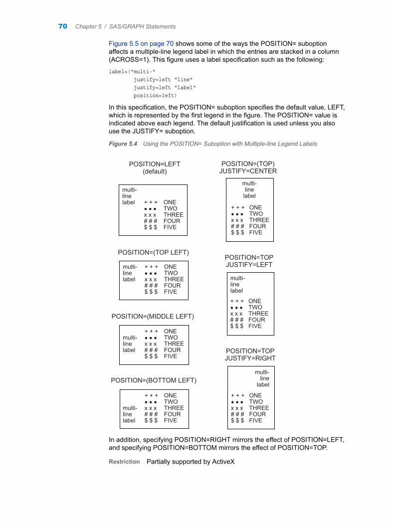
Figure 5.5 on page 70 shows some of the ways the POSITION= suboption affects a multiple-line legend label in which the entries are stacked in a column (ACROSS=1). This figure uses a label specification such as the following:
label=("multi-" justify=left "line" justify=left "label" position=left)
In this specification, the POSITION= suboption specifies the default value, LEFT, which is represented by the first legend in the figure. The POSITION= value is indicated above each legend. The default justification is used unless you also use the JUSTIFY= suboption.
Figure 5.4 Using the POSITION= Suboption with Multiple-line Legend Labels
POSITION=LEFT(default)
POSITION=(TOP)JUSTIFY=CENTER
multi-linelabel + + + ONE ● ● ● TWO x x x THREE # # # FOUR $ $ $ FIVE
POSITION=(TOP LEFT)
multi- + + + ONEline ● ● ● TWOlabel x x x THREE # # # FOUR $ $ $ FIVE
POSITION=(MIDDLE LEFT)
+ + + ONEmulti- ● ● ● TWOline x x x THREElabel # # # FOUR $ $ $ FIVE
POSITION=(BOTTOM LEFT)
+ + + ONE ● ● ● TWOmulti- x x x THREEline # # # FOURlabel $ $ $ FIVE
multi-linelabel
+ + + ONE ● ● ● TWO x x x THREE # # # FOUR $ $ $ FIVE
POSITION=TOPJUSTIFY=LEFT
+ + + ONE ● ● ● TWO x x x THREE # # # FOUR $ $ $ FIVE
multi-linelabel
multi-line
label
+ + + ONE ● ● ● TWO x x x THREE # # # FOUR $ $ $ FIVE
POSITION=TOPJUSTIFY=RIGHT
In addition, specifying POSITION=RIGHT mirrors the effect of POSITION=LEFT, and specifying POSITION=BOTTOM mirrors the effect of POSITION=TOP.
Restriction Partially supported by ActiveX
70 Chapter 5 / SAS/GRAPH Statements

ROTATE=degreesspecifies the angle at which each character of text is rotated with respect to the baseline of the text string. A positive value for degree rotates the character counterclockwise; a negative value moves it clockwise. By default, ROTATE=0 (parallel to the baseline).
Note: Some settings of ROTATE= in the LEGEND statement might result in undesirable text positioning.
Alias R=
Restriction Not supported by ActiveX
See “ANGLE=degrees” on page 68
TICK=nspecifies the nth legend entry. The TICK= suboption is used only with the VALUE= option to designate the legend entry whose text and appearance you want to modify. For example, to change the text of the third legend entry to Minneapolis, specify the following code:
value=(tick=3 "Minneapolis")
The characteristics of all other value descriptions remain unchanged.
If you use the TICK= suboption when you designate text for one legend entry, you must also use it when you designate text for any additional legend entries. For example, this option changes the text of both the second and third legend entries:
value=(tick=2 "Paris" tick=3 "Sydney")
If you omitted TICK=3, the text of the second legend entry would be ParisSydney.
Text description suboptions that precede the TICK= suboption affect all the value descriptions for the legend unless the same suboption (with a different value) follows a TICK= specification. Text description suboptions that follow the TICK= suboption affect only the specified legend entry. For example, suppose you specify this option for a legend with three entries:
value=(color=red font=swiss tick=2 color=blue)
The text of all three entries would use the Swiss font; the first and third entries would be red and only the second entry would be blue.
Alias T=
Details
Description: LEGEND StatementLEGEND statements specify the characteristics of a legend but do not create legends. The characteristics are as follows:
n the position and appearance of the legend box
LEGEND Statement 71

n the text and appearance of the legend label
n the appearance of the legend entries, including the size and shape of the legend values
n the text of the labels for the legend values
LEGEND definitions are not automatically applied when a procedure generates a legend. Instead, they must be explicitly assigned with a LEGEND= option in the appropriate procedure statement.
The following figure illustrates the terms associated with the various parts of a legend.
Figure 5.5 Parts of a Legend
LegendLabel
LegendValue
LegendEntry
OriginOffset
LegendFrame
Legend ValueDescription
Graph Border
Department Parts Repairs Tools
Using Text Description SuboptionsText description suboptions affect all the strings that follow them unless the suboption is changed or turned off. If the value of a suboption is changed, the new value affects all the text strings that follow it. Consider this example:
label=(font=albany amt height=4 "Weight" justify=right height=3 "(in tons)")
FONT=ALBANY applies to both Weight and (in tons). HEIGHT=4 affects Weight, but is respecified as HEIGHT=3 for (in tons). JUSTIFY=RIGHT affects only (in tons).
Using the LEGEND StatementLEGEND statements can be located anywhere in your SAS program. They are global and remain in effect until canceled or until you end your SAS session. LEGEND statements are not applied automatically, and must be explicitly assigned by an option in the procedure that uses them.
You can define up to 99 different LEGEND statements. If you define two LEGEND statements of the same number, the most recently defined statement replaces the previously defined statement of the same number. A LEGEND statement without a number is treated as a LEGEND1 statement.
Cancel individual LEGEND statements by defining a LEGEND statement of the same number without options (a null statement):
legend4;
Canceling one LEGEND statement does not affect any other LEGEND definitions. To cancel all current LEGEND statements, use RESET= in a GOPTIONS statement:
goptions reset=legend;
72 Chapter 5 / SAS/GRAPH Statements

Specifying RESET=GLOBAL or RESET=ALL cancels all current LEGEND definitions as well as other settings.
To display a list of current LEGEND definitions in the SAS LOG window, use the GOPTIONS procedure with the LEGEND option:
proc goptions legend nolist;run;
Positioning the Legend
How to Position a LegendBy default, the legend shares the procedure output area with the procedure output, such as a map or bar chart. See “How Graphics Elements Are Placed in the Graphics Output Area” in SAS/GRAPH: Reference. However, several LEGEND statement options enable you to position a legend anywhere on the graphics output area and even to overlay the procedure output. This section describes these options and their effect on each other.
Positioning the Legend on the Graphics Output AreaThere are two ways that you can position the legend on the graphics output area:
n Describe the general location of the legend with the POSITION= option. If necessary, fine-tune the position with the OFFSET= option.
n Position the legend explicitly with the ORIGIN=option.
Using POSITION= and OFFSET=The values of the POSITION= option affect the legend in two ways:
n OUTSIDE and INSIDE determine whether the legend is located outside or inside the axis area.
n BOTTOM or MIDDLE or TOP (vertical position) and LEFT or CENTER or RIGHT (horizontal position) determine where the legend is located in relation to its OUTSIDE or INSIDE position.
Figure 5.7 on page 74 shows the legend positions inside the axis area.
LEGEND Statement 73

Figure 5.6 Legend Positions inside the Axis Area
Axis LegendPositions
Figure 5.8 on page 74 shows legend positions outside the axis area.
Figure 5.7 Legend Positions outside the Axis Area
LegendPositions
Axis Frame
Axis Area
The default combination is POSITION=(BOTTOM CENTER OUTSIDE). The combination (OUTSIDE MIDDLE CENTER) is not valid.
Use OFFSET=(x,y) to adjust the position of the legend specified by the POSITION= option. The x value shifts the legend either left or right and the y value shifts the legend either up or down.
The offset values are always applied after the POSITION= request. For example, if POSITION=(TOP RIGHT OUTSIDE), the legend is located in the upper right corner of the graphics output area. If OFFSET=(0,0) is specified, the legend does not move. If OFFSET=(–5,–8)CM, the legend moves 5 centimeters to the left and 8 centimeters down.
Using ORIGIN=Use ORIGIN=(x,y) to specify the coordinates of the exact location of the lower left corner of the legend box. Because ORIGIN=(0,0) is the lower left corner of the graphics output area, the values of x and y must be positive. If you specify negative values, a warning is issued and the default value is used.
74 Chapter 5 / SAS/GRAPH Statements

Relating Legends to Other Graphics ElementsBy default, the legend is inside the procedure output area and the space that it occupies reduces the size of the graph itself. If a choice must be made between displaying the legend or the graph, the legend is suppressed. To control how the legend relates to the other elements of the graph, use the MODE= option. These are values for the MODE= option:
n RESERVE reserves space for the legend outside the axis area and moves the graph to make room for the legend. This is the default setting and is valid only when POSITION=OUTSIDE.
n PROTECT prevents the legend from being overwritten by the procedure output. PROTECT blanks out graphics elements, allowing only legend elements to be displayed in the legend's space.
n SHARE displays both graphics elements and legend elements in the same space. This setting is usually used when the legend is positioned inside the axis area. SHARE is useful when the graph has a space that the legend can fit into.
Interactions between POSITION= and MODE=You cannot specify both POSITION=INSIDE and MODE=RESERVE because MODE=RESERVE assumes that the legend is outside the axis area, and POSITION=INSIDE positions the legend inside the axis area. Therefore, when you specify POSITION=INSIDE, change the value of the MODE= option to SHARE or PROTECT. Otherwise, SAS/GRAPH issues a warning and automatically changes the MODE= value to PROTECT.
Creating Drop Shadows and Block EffectsYou can produce a drop shadow or a three-dimensional block effect behind the legend. Use the CSHADOW= or CBLOCK= option in the LEGEND statement in conjunction with the graphics option OFFSHADOW=(x,y).
The value of x determines how far the shadow or block extends to the right (positive numbers) or to the left (negative numbers) of the legend. The value of y determines how far the shadow or block extends above (positive numbers) or below (negative numbers) the legend. If OFFSHADOW=(0,0) is specified, the shadow or block is not visible.
By default, OFFSHADOW=(0.0625, -0.0625) IN. That is, the shadow or block extends 1/16th of an inch to the right and 1/16th of an inch below the legend.
Substituting BY Line Values in a Text StringThe BY statement produces a BY line that contains the variable name and its value. If you specify the variable name, options are available to substitute the variable name and its value in text strings. To use the #BYVAR and #BYVAL options, insert the option in the text string at the position that you want the substitution text to appear. Both #BYVAR and #BYVAL specifications must be followed by a delimiting character. This can be either a space or other nonalphanumeric character, such as the quotation mark that ends the text string. If not, the specification is completely ignored and its text remains intact and is displayed with the rest of the string.
LEGEND Statement 75

To allow a #BYVAR or #BYVAL substitution to be followed immediately by other text, with no delimiter, use a trailing dot (as with macro variables). The trailing dot is not displayed in the resolved text.
If you want a period to be displayed as the last character in the resolved text, use two dots after the #BYVAR or #BYVAL substitution.
The substitution for #BYVAL or #BYVAR does not occur if the following is true:
n The BY statement does not name the variable specified by #BYVAL or #BYVAR. For example, #BYVAL2 when there is only one BY variable or #BYVAL(ABC) when ABC is not a BY variable or does not exist.
n There is no BY statement at all.
When substitution does not occur, no error or warning message is issued and the option specification is displayed with the rest of the string. The graph continues to display a BY line at the top of the page unless you suppress it by using the NOBYLINE option in an OPTION statement.
For more information, see the “BY Statement” on page 49.
Note: This feature is not available in the Annotate facility because BY lines are not created in a DATA step.
NOTE StatementWrites lines of text in the output.
Type: Local
Restriction: Not supported by ActiveX
Note: This local statement has limited use with the GMAP procedure or other procedures. The specified note appears behind the map or graph output by default. With some manipulation of coordinates, notes are useful around the perimeter or ocean area of a map.
Tip: By drawing a white box in back of a note, that boxed note can appear on top of the graph instead of behind it. Here is an example of code that outputs a note on top of a map and a note on top of a chart.
filename odsout '.';
goptions device=png; goptions cback=white;
ODS LISTING CLOSE;ODS HTML path=odsout body="map01.htm" style=htmlblue;
title "Note Text On a Map";pattern1 v=s color=tan;
proc gmap data=mapsgfk.us map=mapsgfk.us;note move=(2,32)pct font="albany amt/bold" height=4pct color=white box=1 blank=yes color=black "Note with 'box' behind it displays on top of map";
76 Chapter 5 / SAS/GRAPH Statements

id state;choro state / levels=1 nolegend;run;
title "Note Text On a Chart";proc gchart data=maps.us;note move=(2,50)pct font="albany amt/bold" height=4pct color=white box=1 blank=yes color=black "Note with 'box' behind it displays on top of chart";hbar state / type=freq levels=7;run;quit;ODS HTML CLOSE;ODS LISTING;
See: “TITLE (global) Statement, FOOTNOTE (global) Statement, NOTE (local) Statement” on page 93
SyntaxNOTE <text-arguments(s)>;
ODS HTML StatementOpens or closes the HTML destination.
Used by: GMAP
Requirement: On mainframes, either GPATH= or PATH= is required.
SyntaxODS HTML <(<ID=> identifier)> <<action> | <option(s)>>;
Details
Description: ODS HTML StatementThis section describes the ODS HTML statement as it relates to SAS/GRAPH procedures. For complete information about the ODS HTML statement, see the SAS Output Delivery System: User’s Guide.
The ODS HTML statement opens or closes the HTML destination. This destination is the default output destination for the Windows and UNIX operating systems. When the destination is open, the procedure produces output that is written in Hypertext Markup Language in the form of an HTML file. If no device is specified,
ODS HTML Statement 77

SAS/GRAPH by default, creates a PNG file containing the graph. The HTML file references the PNG file in order to display the graph in a web page.
SAS/GRAPH adds data tip text to some graphs depending on the device specified. These data tips are generated by default using the values of fields in a SAS data set. You can specify the DESCRIPTION= option on the SAS/GRAPH procedure to change or remove the data tip text. For more information about using data tips see “Data Tips for Web Presentations” in SAS/GRAPH: Reference.
The FILE= option identifies the file that contains the HTML version of the procedure output. With SAS/GRAPH, the body file contains references to the graphs. If DEVICE=PNG, the graphs are stored in separate PNG files. When you view the body file in a browser, the graphs are automatically displayed. By default with ODS processing, both the HTML and PNG files are stored in the current WORK library. To specify a destination for all the HTML and PNG files, use the PATH= option. You can store the PNG files in a different location than the HTML files. Use the GPATH= option to specify a location for the PNG files, and the PATH= option to specify the location of the HTML files. In both cases, the destination must be an aggregate storage location.
AnchorsODS HTML automatically creates an anchor for every piece of output generated by the SAS procedures. An anchor specifies a particular location within an HTML file. In SAS/GRAPH, an anchor usually defines a link target such as a graph whose location is defined in an IMG element.
In order for the links from the contents, page, or frame file to work, each piece of output in the body files must have a unique anchor to link to. The anchor for the first piece of output in a body file acts as the anchor for that file. These anchors are used by the frame and contents files, if they are created, to identify the targets for the links that ODS HTML automatically generates. For more information about using anchors with the ODS HTML statement, see the SAS Output Delivery System: User’s Guide.
You can specify a name for an HTML anchor with the following code:
ods html anchor="string";
This enables you to link directly to that identifying name.
PATTERN StatementDefines the characteristics of patterns used in maps.
Used by: GMAP
Type: Global
SyntaxPATTERN<1 …255><COLOR=pattern-color | _style_><IMAGE=fileref | "external-file">
78 Chapter 5 / SAS/GRAPH Statements

<IMAGESTYLE=TILE | FIT><REPEAT=number-of-times><VALUE=block-pattern | map-pattern >;
Optional ArgumentsCOLOR=pattern-color | _style_
specifies the color of the fill. Pattern-color is any SAS/GRAPH color name. The _STYLE_ value specifies the appropriate color based on the current style. See “Using Colors in SAS/GRAPH Programs” in SAS/GRAPH: Reference.
Using the COLOR= option with a null value cancels the color specified in a previous PATTERN statement of the same number without affecting the values of other options.
The COLOR= option overrides the CPATTERN= graphics option.
The CFILL= option in the PIE and STAR statements overrides the COLOR= option. For details, see “Controlling Slice Patterns and Colors” in SAS/GRAPH: Reference.
No color can be specified for a PATTERN statement, that is, neither the COLOR= nor the CPATTERN= option is used. In this case the PATTERN statement rotates the specified fill through each color in the color list before the next PATTERN statement is used.
Alias C=
Restriction Partially supported by ActiveX
See “Working with PATTERN Statements” on page 89
Example “Using BY-group Processing to Generate a Series of Charts” in SAS/GRAPH: Reference
CAUTION Omitting the COLOR= option in a PATTERN statement can cause the PATTERN statement to generate multiple PATTERN definitions.
IMAGE=fileref | "external-file"specifies an image file that is used to fill one or more areas of a map. The format of the external file specification varies across operating environments. See the companion reference for your specific operating environment.
Restriction Partially supported by ActiveX
Notes When you specify an image file to fill a map, the map is not outlined. Also, the COLOR= and VALUE= options are ignored.
For DEVICE=ACTIVEX and DEVICE=ACTXIMG, if you do not specify a pathname to the image, then the ActiveX control searches a predefined list of locations to try to find the image. If all else fails, the ActiveX control looks for the image on the web. It is recommended that you specify the pathname to the image.
See “IMAGESTYLE=TILE | FIT” on page 80
PATTERN Statement 79

IMAGESTYLE=TILE | FITspecifies how the image specified in the IMAGE= option is to be applied to fill a map. The TILE value repeats the image as needed to fill the map. The FIT value stretches a single instance of the image to fill the map.
Default TILE
Restriction Partially supported by ActiveX
REPEAT=number-of-timesspecifies the number of times that a PATTERN definition is applied before the next PATTERN definition is used.
The behavior of the REPEAT= option depends on the color specification:
n If you use both the COLOR= and REPEAT= options in a PATTERN statement, the pattern is repeated the specified number of times in the specified color. The fill can be either the default solid or a fill specified with the VALUE= option.
n You can use the CPATTERN= option in a GOPTIONS statement to specify a single pattern color. Use the REPEAT= option either alone or with the VALUE= option in a PATTERN statement. The resulting hatch pattern is repeated the specified number of times.
n You can omit both the COLOR= and CPATTERN= options and use the REPEAT= option. If you use the REPEAT= option alone, it generates default solids. Or you can use the REPEAT= option in conjunction with the VALUE= option in a PATTERN statement. The resulting pattern is rotated through each color in the color list. The entire group generated by this cycle is then repeated the number of times specified in the REPEAT= option. Thus, the total number of patterns produced depends on the number of colors in the current color list.
Using REPEAT= with a null value cancels the repetition specified in a previous PATTERN statement of the same number without affecting the values of other options. Note that in most cases, it is preferable to use LEVELS=1 in the GMAP procedure rather than using this option in the PATTERN statement.
Alias R=
Default REPEAT=1
Restriction Partially supported by ActiveX
See “Understanding Pattern Sequences” on page 91
VALUE=block-patternPatterns are specified for the blocks in block maps produced by the BLOCK statement in the GMAP procedure. (The map area from which the block rises takes a map pattern as described in the option “VALUE= map-pattern” on page 82.) See also “About Block Maps and Patterns” on page 300.
Values for block-pattern are as follows:
EMPTYan empty pattern. The ActiveX control does not support EMPTY.
Alias E
80 Chapter 5 / SAS/GRAPH Statements

SOLIDa solid pattern (the only valid value for three-dimensional charts).
Alias S
style<density>a shaded pattern. Style specifies the direction of the lines:
Lspecifies left-slanting lines.
Rspecifies right-slanting lines.
Xspecifies crosshatched lines.
Density specifies the density of the pattern's shading. Specify a number from 1 to 5. The number 1 produces the lightest shading and 5 produces the heaviest shading.
Note: style<density> is not supported by the ActiveX device driver.
Figure 5.9 on page 81 shows all of the patterns available for bars and blocks.
Figure 5.8 Bar and Block Patterns
R
X
L
E 1 2 3 4 5 S
If no valid patterns are available, default bar and block fill patterns are selected in this order:
1 SOLID
2 X1–X5
PATTERN Statement 81

3 L1–L5
4 R1–R5
Each fill is used once with every color in the color list unless a pattern color is specified. The entire sequence is repeated as many times as required to provide the necessary number of patterns.
Alias V=
Restriction Partially supported by ActiveX
VALUE= map-patternspecifies patterns for the following:
The VALUE= option specifies patterns for map area surfaces in block, choropleth, and prism maps produced by the BLOCK, CHORO, AND PRISM statements in the GMAP procedure.
Values for map-pattern are as follows:
MEMPTYspecifies an empty pattern.
Alias ME
Restriction EMPTY or E are not valid aliases when used with the map areas in block maps created by the GMAP procedure.
MSOLIDspecifies a solid pattern.
Alias MS
Restriction SOLID or S are not valid aliases when used with the map areas in block maps created by the GMAP procedure.
Mdensity<style<angle>>specifies a shaded pattern.
Density specifies the density of the pattern's shading. Specify a number from 1 to 5. The number 1 produces the lightest shading and 5 produces the heaviest shading.
Style specifies the type of the pattern lines:
Nspecifies parallel lines (the default).
Xspecifies crosshatched lines.
Angle specifies the angle of the pattern lines. Specify a number from 0 to 360. The number specifies the degrees at which the parallel lines are drawn, measured from the horizontal. By default, angle is 0 (lines are horizontal).
Note Mdensity<style<angle>> is not supported by the ActiveX device driver.
Figure 5.10 on page 83 shows some typical plot patterns.Figure 5.10 on page 83 shows some typical map patterns.
82 Chapter 5 / SAS/GRAPH Statements

Figure 5.9 MapPatterns
M3N0 M3X0
M3N90 M3X90
M3X135M3N135
M3N45 M3X45
0º
45º
90º
135º
If no valid patterns are available, default plot fill patterns are selected in this order:
1 MSOLID
2 M2N0
3 M2N90
4 M2X45
5 M4N0
6 M4N90
7 M4X90
Each fill is used once with every color in the color list unless a pattern color is specified. The entire sequence is repeated as many times as required to provide the necessary number of patterns.
Alias V=
Restriction Partially supported by ActiveX
PATTERN Statement 83

VALUE=pie/star-patternspecifies patterns for pie and star charts produced by the PIE and STAR statements in the GCHART procedure. Values for pie/star-pattern are as follows:
PEMPTYspecifies an empty pattern. EMPTY or E are also valid aliases.
Alias PE
PSOLIDspecifies a solid pattern. SOLID or S are also valid aliases.
Alias PS
Pdensity<style<angle>>specifies a shaded pattern.
Density specifies the density of the pattern's shading. Specify a number from 1 to 5. The number 1 produces the lightest shading and 5 produces the heaviest shading.
Style specifies the type of the pattern lines:
Nspecifies parallel lines (the default).
Xspecifies crosshatched lines.
Angle specifies the angle of the pattern lines. Specify a number from 0 to 360. The number specifies the angle of the lines, measured in degrees from perpendicular to the radius of the slice. By default, angle is 0.
Note Pdensity<style<angle>> is not supported by the ActiveX device driver.
The FILL= option in the PIE and STAR statements in the GCHART procedure overrides VALUE=.
Figure 5.11 on page 85 shows some typical pie and star patterns.
84 Chapter 5 / SAS/GRAPH Statements
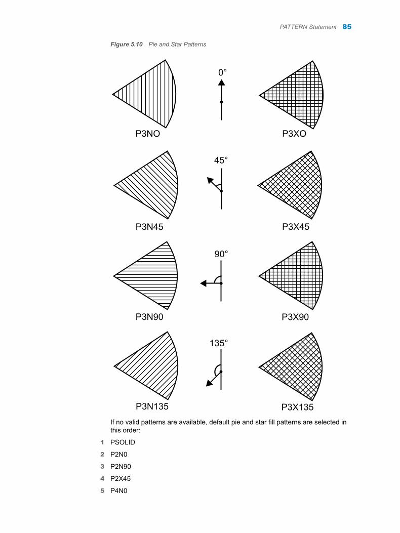
Figure 5.10 Pie and Star Patterns
P3NO P3XO
P3N45 P3X45
P3N90 P3X90
P3N135 P3X135
•
0°
•
45°
•
90°
•
135°
If no valid patterns are available, default pie and star fill patterns are selected in this order:
1 PSOLID
2 P2N0
3 P2N90
4 P2X45
5 P4N0
PATTERN Statement 85

6 P4N90
7 P4X90
Each fill is used once with every color in the color list unless a pattern color is specified. The entire sequence is repeated as many times as required to provide the necessary number of patterns.
Alias V=
Restriction Partially supported by ActiveX
Note If you use hatch patterns and request a legend instead of slice labels, the patterns in the slices are oriented to be visually equivalent to the legend.
Details
Description: PATTERN StatementPATTERN statements create PATTERN definitions that define the color and type of area fill for patterns used in maps. This is the procedure and the graphics areas that it creates that use PATTERN definitions:
GMAPmap areas in choropleth, block, and prism maps; blocks in block maps
In addition, certain Annotate facility functions and macros can use pattern specifications. and “Using Annotate Data Sets” in SAS/GRAPH: Reference.
You can use the PATTERN statement to control the fill and color of a pattern, and whether the pattern is repeated. There are various types of patterns:
n block patterns
n map patterns
Pattern fills can be solid or empty, or composed of parallel or crosshatched lines. In addition, you can specify device-dependent hardware patterns for polygon fills on devices that support hardware patterns.
If you do not create PATTERN definitions, SAS/GRAPH software generates them as needed and assigns them to your graphs by default. Generally, the default behavior is to rotate a solid pattern through the current color list. For details, see “About Default Patterns” on page 88.
Using the PATTERN Statement
How PATTERN Definitions Are GeneratedPATTERN statements can be located anywhere in your SAS program. They are global and remain in effect until redefined, canceled, or until the end of your SAS session.
86 Chapter 5 / SAS/GRAPH Statements

You can define up to 255 different PATTERN statements. A PATTERN statement without a number is treated as a PATTERN1 statement.
PATTERN statements generate one or more PATTERN definitions, depending on how the COLOR=, VALUE=, and IMAGE= options are used. For information about PATTERN definitions, see “Working with PATTERN Statements” on page 89, as well as the descriptions of “ COLOR=pattern-color | _style_” on page 79, “IMAGE=fileref | "external-file"” on page 79, and “VALUE= map-pattern” on page 82.
PATTERN definitions are generated in the order in which the statements are numbered, regardless of gaps in the numbering or the statement's position in the program. Although it is common practice, you do not have to start with PATTERN1, and you do not have to use sequential statement numbers.
PATTERN definitions are applied automatically to all areas of the graphics output that require patterns. When assigning PATTERN definitions, SAS/GRAPH starts with the lowest-numbered definition with an appropriate fill specification or with no fill specification. It continues to use the specified patterns until all valid PATTERN definitions have been used. Then, if more patterns are required, SAS/GRAPH returns to the default pattern rotation, but continues to outline the areas in the same color as the fill.
Altering or Canceling PATTERN StatementsPATTERN statements are additive. You can define a PATTERN statement and later submit another PATTERN statement with the same number. The new PATTERN statement redefines or cancels only the options that are included in the new statement. Options not included in the new statement are not changed and remain in effect. For example, assume you define PATTERN4 as follows:
pattern4 value=x3 color=red repeat=2;
This statement cancels only REPEAT= without affecting the rest of the definition:
pattern4 repeat=;
Add or change options in the same way. This statement changes the color of the pattern from red to blue:
pattern4 color=blue;
After all these modifications, PATTERN4 has these characteristics:
pattern4 value=x3 color=blue;
Cancel individual PATTERN statements by defining a PATTERN statement of the same number without options (a null statement):
pattern4;
Canceling one PATTERN statement does not affect any other PATTERN definitions. To cancel all current PATTERN statements, use the RESET= option in a GOPTIONS statement:
goptions reset=pattern;
Specifying RESET=GLOBAL or RESET=ALL cancels all current PATTERN definitions as well as other settings.
To display a list of current PATTERN definitions in the LOG window, use the GOPTIONS procedure with the PATTERN option:
proc goptions pattern nolist;run;
PATTERN Statement 87

About Default Patterns
How SAS/GRAPH Generates and Assigns PATTERN DefinitionsWhen a procedure produces a graph that needs one or more patterns, SAS/GRAPH does one of the following actions:
n automatically generates the appropriate default patterns and outlines to fill the areas
n uses patterns, colors, and outlines that are defined by PATTERN statements, graphics options, and procedure options.
In order to understand how SAS/GRAPH generates and assigns patterns defined with PATTERN statements, it is helpful to understand how it generates and assigns default patterns. The following sections describe the default pattern behavior for all procedures. See “Working with PATTERN Statements” on page 89 for details about defining patterns.
How Default Patterns and Outlines Are GeneratedIn general, the default pattern that SAS/GRAPH uses is a solid fill. The default colors are determined by the current style and the device.
SAS/GRAPH uses default patterns when no PATTERN statements are defined. The default colors are determined by the current style and the device.
Because the system option-GSTYLE-is in effect by default, the procedure uses the style's default block fill colors, widths, patterns, and outline colors when producing output. Specifically, SAS/GRAPH uses the default values when you do not specify any of the following:
n any PATTERN statements
n the CPATTERN= graphics option
n the COLORS= graphics options (that is, you use the device's default color list and it has more than one color)
n the COUTLINE= option in the action statement
If all of these conditions are true, then SAS/GRAPH performs the following operations:
n selects the first default fill for the appropriate pattern, which is always solid. It rotates once through the list of colors available in the current style, generating one solid pattern for each color. If you use the default style colors and the first color in the list is either black or white, the procedure does not create a pattern in that color. If you specify a color list with the COLORS= graphics option, then the procedure uses all the colors in the list to generate the patterns.
Note: The one exception to the default solid pattern is the map area pattern in a block map produced by the GMAP procedure, which uses a hatch fill by default. By default the map areas and their outlines use the first color in the color list. This happens regardless of whether the list is the default device list or one specified with COLORS= in the GOPTIONS statement.
88 Chapter 5 / SAS/GRAPH Statements

n uses the style's outline color to outline every patterned area.
If a procedure needs additional patterns, SAS/GRAPH selects the next default pattern fill appropriate to the graph and rotates it through the color list, skipping the foreground color as before. SAS/GRAPH continues in this fashion until it has generated enough patterns for the chart.
Things That Affect Default PatternsChanging any of these conditions can change or override the default behavior:
n If you specify a color list with the COLORS= option in a GOPTIONS statement and the list contains more than one color, SAS/GRAPH rotates the default fills, beginning with SOLID, through that list. In this case, it uses every color, even if the foreground color is black (or white). The default outline color remains the foreground color.
n If you specify either COLORS=(one-color) or the CPATTERN= graphics option, the default fill changes from SOLID to the appropriate list of hatch patterns. SAS/GRAPH uses the specified color to generate one pattern definition for each hatch pattern in the list.
For a description of these options, see “Graphics Options and Device Parameters Dictionary” in SAS/GRAPH: Reference.
Working with PATTERN Statements
What You Can Specify with PATTERN StatementsWith PATTERN statements, you can specify the following:
n the type of fill (VALUE=)
n the color of the fill (COLOR=)
n the images used to fill the bars in a two-dimensional chart (IMAGE=)
n how many times to apply the statement before using the next one (REPEAT=).
You can also use procedure options to specify the pattern outline color and the CPATTERN= graphics option to specify a default color for all patterns.
Whether you use PATTERN statement options alone or with each other affects the number and type of patterns your PATTERN statements generate. Depending on which options you use, you can explicitly specify every pattern used by your graphs. Or you can let the PATTERN statement generate a series of pattern definitions using either the color list or the list of default fills.
Explicitly Specifying PatternsTo explicitly specify all the patterns in your graph, you need to do one of the following for every pattern your graph requires:
n Provide a PATTERN statement that uses the COLOR= option to specify the pattern color, for example:
pattern1 color=red;
PATTERN Statement 89

By default, the fill type is SOLID.
n Provide a PATTERN statement that uses both the COLOR= option and the VALUE= option to specify the fill, for example:
pattern1 color=blue value=r3;
Including the COLOR= option in the PATTERN statement is the simplest way to ensure that you get exactly the patterns that you want. When you use the COLOR= option, the PATTERN statement generates exactly one PATTERN definition for that statement. If you also use the REPEAT= option, the PATTERN definition is repeated the specified number of times.
Generating Multiple Pattern DefinitionsYou can also use PATTERN statements to generate multiple PATTERN definitions. To do this use the VALUE= option to specify the type of fill you want but omit the COLOR= option. For example:
pattern1 value=r3;
In this case, the PATTERN statement rotates the R3 fill through all the colors in the color list. For more information about pattern rotation, see “Understanding Pattern Sequences” on page 91.
Selecting an Appropriate PatternThe type of fill pattern that you specify depends on the type of graph that you are producing:
Table 5.1 Fill Patterns for Graph Types
Type of graph Appropriate type of fill
block maps (PROC GMAP) “ VALUE=block-pattern” on page 80
map area surfaces (PROC GMAP) “VALUE= map-pattern” on page 82
Note: You might specify a fill that is inappropriate for the type of graph that you are generating. For example, you might specify VALUE=L1 in a PATTERN statement for a choropleth map. In this case SAS/GRAPH ignores the PATTERN statement and continues searching for a valid pattern. If it does not find a definition with a valid fill specification, it uses default patterns instead.
Controlling Outline ColorsWhenever you use PATTERN statements, the default outline color uses the style's outline color to outline every patterned area.
You can change the outline color of any pattern, whether the pattern is default or user-defined. Use the COUTLINE= option or the CEMPTY= option, or both, in the action statement that generates the map.
90 Chapter 5 / SAS/GRAPH Statements

The Effect of the CPATTERN= Graphics OptionAlthough the CPATTERN= graphics option is used most often with default patterns, it does affect the PATTERN statement. With default patterns (no PATTERN statements specified), it does the following:
n specifies the color for all patterns
n causes default patterns to use hatched fills instead of the default SOLID
In conjunction with the PATTERN statement that it does the following:
n With a PATTERN statement that specifies only a fill (VALUE=), the CPATTERN= option determines the color of that fill. For example, these statements produce two green, hatched patterns:
goptions cpattern=green;pattern1 value=x3;pattern2 value=x1;
n With a PATTERN statement that specifies only a color (COLOR=), the COLOR= option overrides the CPATTERN= color, but CPATTERN= causes the fill to be hatched, not the default SOLID. For example, these statements produce one red, hatched pattern:
goptions cpattern=green;pattern1 color=red;
See also the description of “CPATTERN Graphics Option” in SAS/GRAPH: Reference.
Understanding Pattern Sequences
About Pattern SequencesPattern sequences are sets of PATTERN definitions that SAS/GRAPH automatically generates when a PATTERN statement specifies a fill but not a color. In this case, the specified fill is used once with every color in the color list. If the REPEAT= option is also used, the resulting PATTERN definitions are repeated the specified number of times.
Generating Pattern SequencesSAS/GRAPH generates pattern sequences when a PATTERN statement uses VALUE= to specify a fill and all of the following conditions are also true:
n The COLOR= option is not used in the PATTERN statement.
n The CPATTERN= graphics option is not used.
n The color list, either default or user-specified, contains more than one color.
In this case, the PATTERN statement rotates the fill specified by the VALUE= option through every color in the color list. One PATTERN definition is generated for every color in the list. After every color has been used once, SAS/GRAPH goes to the next PATTERN statement. For example, suppose you specified the following color list and PATTERN statements for bar or block patterns:
goptions colors=(blue red green) ctext=black;
PATTERN Statement 91

pattern1 color=red value=x3;pattern2 value=r3;pattern3 color=blue value=l3;
Here, PATTERN1 generates the first PATTERN definition. PATTERN2 omits the COLOR= option, so the specified fill is rotated through all three colors in the color list before the PATTERN3 statement is used. This table sequentially lists the color and fill of the PATTERN definitions that would be generated if nine patterns were required:
Table 5.2 Color and Fill PATTERN Definitions for the First Nine Patterns
Definition Number Source
Characteristics
Color Fill
1 PATTERN1 Red x3
2 PATTERN2 Blue r3
3 PATTERN2 Red r3
4 PATTERN2 Green r3
5 PATTERN3 Blue l3
6 First default Blue Solid
7 First default Red Solid
8 First default Green Solid
9 Second default
Blue x1
Notice that after all the PATTERN statements are exhausted, the procedure begins using the default bar and block patterns, beginning with SOLID. Each fill from the default list is rotated through all three colors in the color list before the next default fill is used.
Repeating Pattern SequencesIf you use the REPEAT= option but not the COLOR= option, the sequence generated by cycling the definition through the color list is repeated the number of times specified by the REPEAT= option. For example, these statements illustrate the effect of the REPEAT= option on PATTERN statements both with and without explicit color specifications:
goptions colors=(red blue green);pattern1 color=gold repeat=2;pattern2 value=x1 repeat=2;
In the following table, PATTERN1 is used twice and PATTERN2 cycles through the list of three colors and then repeats this cycle a second time:
92 Chapter 5 / SAS/GRAPH Statements

Table 5.3 The Cyclical Use of PATTERN Statements
Sequence Number Source
Characteristics
Color Fill
1 PATTERN1 Gold Solid (first default)
2 PATTERN1 Gold Solid (first default)
3 PATTERN2 Red x1
4 PATTERN2 Blue x1
5 PATTERN2 Green x1
6 PATTERN2 Red x1
7 PATTERN2 Blue x1
8 PATTERN2 Green x1
TITLE (global) Statement, FOOTNOTE (global) Statement, NOTE (local) StatementControl the content, appearance, and placement of text.
Valid in: Anywhere
Used by: GMAP
Type: TITLE and FOOTNOTE are global statements. NOTE is a local statement.
Restrictions: The cumulative text from the TITLE1-10 statements must not exceed 256 characters for output using the SVG device.Options such as COLOR=, ALT= and LINK= are not supported by the SGMAP procedure.
SyntaxTITLE<1 …10> <text-argument(s)>;
FOOTNOTE<1 …10> <text-argument(s)>;
NOTE<text-arguments(s)>;
TITLE (global) Statement, FOOTNOTE (global) Statement, NOTE (local) Statement 93

Summary of Optional ArgumentsAppearance options
COLOR=color specifies the color for the following text, box, or line.
FONT=fontspecifies the font for the subsequent text.
HEIGHT=text-height<units>specifies the height of text characters in number of units.
Baseline angling and character rotation optionsANGLE=degrees
specifies the angle of the baseline of the entire text string with respect to the horizontal.
LANGLE=degreesspecifies the angle of the entire text-string(s).
ROTATE=degreesspecifies the angle at which each character of text is rotated.
Boxing, underlining, and line drawing optionsBCOLOR=background-colorBLANK=YES
protects the box and its contents from being overwritten by any subsequent graphics elements.
BOX=1 …4 draws a box around one line of text.
BSPACE=box-space<units>specifies the amount of space between the boxed text and the box.
DRAW=(x,y …,x-n,y-n)<units>draws lines anywhere on the graphics output area.
UNDERLIN=0 …3underlines subsequent text.
Linking optionALT="text-string"
specifies descriptive text for a URL to which a title or footnote links, or the title or footnote itself.
LINK="URL"specifies a uniform resource locator (URL) to which a title or footnote links.
Placement and spacing optionsJUSTIFY=LEFT | CENTER | RIGHT
specifies the alignment of the text string.LSPACE=line-space <units>
specifies the amount of spacing above and below lines of text.MOVE=(x,y) <units>
positions a text string.WRAP
wraps the text to a second line if the text does not fit on one line.
94 Chapter 5 / SAS/GRAPH Statements

Text provision optiontext-string(s)
is an element of text-argument(s) and specifies one or more strings up to 512 characters. Any of the following text-options that are used to modify a text-string must precede text-string.
Optional Argumentstext-arguments(s) can be one or more of "text-string" and text-options. Text options must precede the "text-string" that they modify. text-options can be one or more of the following optional arguments, in any order:
ALT="text-string"specifies descriptive text for a URL to which a title or footnote links, or the title or footnote itself. The "text-string" that you use to describe a title or a footnote, or the URL specified by the LINK= option, can contain occurrences of the variables #BYVAL, #BYVAR, and #BYLINE, as described in “ text-string(s)” on page 107.
Supports The ALT= option can be used in conjunction with the LINK= option.
Note The title or footnote can be displayed by using an ODS markup destination (such as HTML). Also, the corresponding ODS option NOGTITLE or NOGFOOTNOTE is specified. In this case, the title or footnote is rendered in the body of the HTML file rather than in the graphic itself. And the ALT= text is not associated with the title or footnote.
See “Controlling Where Titles and Footnotes Are Rendered” in SAS/GRAPH: Reference
“ LINK="URL"” on page 104
Example “Example 11: Using Traditional Map Data to Produce a Drilldown Choropleth Map” on page 379
ANGLE=degreesspecifies the angle of the baseline of the entire text string with respect to the horizontal. A positive degrees value angles the baseline counterclockwise; a negative value angles it clockwise. By default, ANGLE=0 (horizontal).
Angled titles or footnotes might require more vertical space. Consequently, there might be an increase the size of the title area or the footnote area, thereby reducing the vertical space in the procedure output area.
Using the BOX= option with angled text does not produce angled boxes; the box is sized to accommodate the angled note.
Using the ANGLE= option after one text string and before another can reset some options to their default values. See “Using Options That Can Reset Other Options” on page 111.
The ANGLE= option has the same effect on the text as LANGLE=, except when you specify an angle of 90 degrees or –90 degrees. In these angle specifications, the procedure output area is shrunk from the left or right to accommodate the angled title or footnote. The result depends on the statement in which you use the option:
n With the TITLE statement:
TITLE (global) Statement, FOOTNOTE (global) Statement, NOTE (local) Statement 95
Figure 5.12 on page 96 shows how ANGLE=90-degrees or ANGLE=–90-degrees positions and rotates the title text.
ANGLE=90 positions the title at the left edge of the graphics output area, angled 90 -degrees (counterclockwise) and centered vertically.
ANGLE=–90 positions the title at the right edge of the graphics output area, angled –90-degrees (clockwise) and centered vertically.
Figure 5.11 Positioning Titles with the ANGLE= OptionTi
tle w
ith A
NG
LE=9
0Title w
ith AN
GLE
=−90
n With the FOOTNOTE statement:
Figure 5.13 on page 96 shows how ANGLE=90 degrees or ANGLE=–90 degrees positions and rotates footnote text.
ANGLE=90 positions the footnote at the right edge of the graphics output area, angled 90 degrees (counterclockwise) and centered vertically.
ANGLE=–90 positions the footnote at the left edge of the graphics output area, angled –90 (clockwise) and centered vertically.
Figure 5.12 Positioning Footnotes with the ANGLE=Option
F ootnote with A
NG
LE=
− 90 Foot
note
with
AN
GLE
=90
n With the NOTE statement:
Figure 5.14 on page 97 shows how ANGLE= 90 degrees or -90 degrees positions and rotates note text.
96 Chapter 5 / SAS/GRAPH Statements

ANGLE=90 positions the note at the bottom of the left edge of the graphics output area, angled 90 degrees (counterclockwise) and reading from bottom to top.
ANGLE=–90 positions the note at the top of the right edge of the graphics output area, angled –90 (clockwise) and reading from top to bottom.
Figure 5.13 Positioning Notes with the ANGLE= Option
Not
e w
ith A
NG
LE=9
0
Note w
ith AN
GLE
=−90
Footnote
Title
Alias A=
Restriction Not supported by ActiveX
See “ LANGLE=degrees” on page 103
“ ROTATE=degrees” on page 106
Example “Example 1: Enhancing Titles” on page 113
BCOLOR=background-colorspecifies the background color of a box produced by the BOX= option. By default, the background color of the box is the same as the background color for the entire graph. The color of the frame of the box is determined by the color specification used in BOX=.
Alias BC=
Restriction If you omit BOX=, BCOLOR= is ignored.
Note The BCOLOR= option can be reset by the ANGLE= or JUSTIFY= options, or by the MOVE= option with absolute coordinates.
See “Using Options That Can Reset Other Options” on page 111 for details
“ BOX=1 …4 ” on page 98
Example “Example 1: Enhancing Titles” on page 113
BLANK=YESprotects the box and its contents from being overwritten by any subsequent graphics elements. It does this by blanking out the area where the box is displayed. The BLANK= option enables you to overlay graphics elements with boxed text. It is ignored if you omit the BOX= option. Because titles and
TITLE (global) Statement, FOOTNOTE (global) Statement, NOTE (local) Statement 97

footnotes are written from the highest numbered to the lowest numbered, the BLANK= option only blanks out titles and footnotes of a lower number.
Alias BL=
Restriction Not supported by ActiveX
Note The BLANK= option can be reset by the ANGLE= or JUSTIFY= options, or by the MOVE= option with absolute coordinates.
See “Using Options That Can Reset Other Options” on page 111 for details
“ BOX=1 …4 ” on page 98
Example “Example 1: Enhancing Titles” on page 113
BOX=1 …4draws a box around one line of text. A value of 1 produces the thinnest box lines; 4 produces the thickest. Boxing angled text does not produce an angled box; the box is sized to include the angled text.
The color of the box is one of the following:
n the color specified by the COLOR= option in the statement
n the default text color
The COLOR= option, preceding the BOX= option, controls the box frame color. To color the background of the box, use the BCOLOR= option. Specify the same color with both the COLOR= option and the BCOLOR= option to effect a box without a frame.
You can include more than one text string in the box as long as no text break occurs between the strings. That is, you cannot use the JUSTIFY= option to create multiple lines of text within a box.
To draw a box around multiple lines of text, you can do either of the following:
n Use the MOVE= option with relative coordinates to position an additional line of text relative to the preceding line and enclose them within the box drawn by the BOX= option. For example, this statement produces the boxed note shown in Figure 5.15 on page 99:
note font=swiss justify=center box=1 "Office Hours" move=(-7,-2)pct "9-5";
The MOVE=option in this NOTE statement overrides the JUSTIFY= option that center-positioned the first line of text. The MOVE= option specifies the x and y coordinates in percentage units. The text string ‘9–5’ is positioned relative to the first text string ‘Office Hours’.
Using the MOVE= option in a NOTE statement enables you to position a note on top of a graph. See the “NOTE Statement” for a code sample.
n Use the DRAW= option to draw the box and do not use the BOX= option.
98 Chapter 5 / SAS/GRAPH Statements

Figure 5.14 Using the BOX= Option and the MOVE= Option to Box Multiple Lines of Text
Alias BO=
Restriction Not supported by ActiveX
Note The BOX= option can be reset by the ANGLE= or JUSTIFY= options, or by the MOVE= options with absolute coordinates.
See “Using Options That Can Reset Other Options” on page 111 for details
“ BCOLOR=background-color” on page 97
“ BLANK=YES ” on page 97
“ BSPACE=box-space<units>” on page 99
Example “Example 1: Enhancing Titles” on page 113
BSPACE=box-space<units>specifies the amount of space between the boxed text and the box. The space above the text is measured from the font maximum, and the space below the text is measured from the font minimum. By default, BSPACE=1.
The spacing is uniform around the box. Notice that BSPACE=.5IN leaves one-half inch of space between the text and the top, bottom, and sides of the box.
Alias BS=
Restriction Not supported by ActiveX
Interaction If the BOX= option is not used, the BSPACE= option is ignored
Note The BSPACE= option can be reset by the ANGLE= or JUSTIFY= options, or by the MOVE= option with absolute coordinates.
See “Using Options That Can Reset Other Options” on page 111 for details
“ BOX=1 …4 ” on page 98
TITLE (global) Statement, FOOTNOTE (global) Statement, NOTE (local) Statement 99

COLOR=colorspecifies the color for the following text, box, or line. The COLOR= option affects all text, lines, and boxes that follow it and stays in effect until another COLOR= specification is encountered.
Change colors as often as you like. For example, this statement produces a title with red text in a box with a blue frame and a cream background:
title color=red "Total Sales" color=blue box=3 bcolor=cream;
Although the BCOLOR= option controls the background color of the box, the frame color is controlled with the COLOR= option that precedes the BOX= option.
If you omit the COLOR= option, a color specification is searched for in this order:
1 the CTITLE= option in a GOPTIONS statement
2 the CTEXT= option in a GOPTIONS statement
3 the default, the first color in the color list.
Alias C=
Style reference Color attribute of the GraphTitle1Text (TITLE1) and the GraphTitleText (TITLE2...n) elements
See “ BCOLOR=background-color” on page 97
“Controlling Titles and Footnotes” in SAS/GRAPH: Reference
DRAW=(x,y …,x-n,y-n)<units>draws lines anywhere on the graphics output area. Lines are drawn using x and y as absolute or relative coordinates. The following table shows the specifications for absolute and relative coordinates:
Table 5.4 Coordinate Specifications
Absolute Coordinates Relative Coordinates
x<units> ±x<units>
y<units> ±y<units>
The coordinate position (0,0) is the lower left corner of the graphics output area. Specify at least two coordinate pairs. Commas between coordinates are optional; blanks can be used instead. The DRAW= option does not affect the positioning of text.
The starting point for lines specified with relative coordinates begins at the end of the most recently drawn text or line in the current statement. If no text or line has been drawn in the current statement, a warning is issued. The relative draw is measured from where a zero-length text string would have ended, given the normal placement for the statement.
You can mix relative and absolute coordinates. For example, DRAW=(+0,+0,+0,1IN) draws a vertical line from the end of the text to one inch from the bottom of the graphics output area.
100 Chapter 5 / SAS/GRAPH Statements

Alias D=
Restriction Not supported by ActiveX
Example “Example 1: Enhancing Titles” on page 113
FONT=fontspecifies the font for the subsequent text. See “Specifying Fonts in SAS/GRAPH Programs” in SAS/GRAPH: Reference for details about specifying SAS/GRAPH fonts. If you omit this option, a font specification is searched for in this order:
n for a TITLE1 statement:
1 the FTITLE= option in a GOPTIONS statement
2 the FTEXT= option in a GOPTIONS statement
3 the default font, SWISS (COMPLEX in Release 6.06 and earlier)
n for all other TITLE statements and the FOOTNOTE and NOTE statements:
1 the FTEXT= option in a GOPTIONS statement
2 the default hardware font, NONE
Alias F=
Style reference
Font attribute of the GraphTitle1Text (TITLE1) and the GraphTitleText (TITLE2...n) elements
Notes Font names greater than eight characters in length must be enclosed in quotation marks.
If the TITLE or FOOTNOTE is displayed using an ODS markup destination and the corresponding NOGTITLE or NOGFOOTNOTE option is specified, then the bold and italic FONT attributes are on by default. However, if you specify different attributes with the FONT= option, the bold and italic attributes are turned off.
See “Controlling Titles and Footnotes” in SAS/GRAPH: Reference
Example “Example 1: Enhancing Titles” on page 113
HEIGHT=text-height<units>specifies the height of text characters in number of units.
Height is measured from the font minimum to the capline. Ascenders can extend above the capline, depending on the font.
If your text line is too long to be displayed in the height specified in the HEIGHT= option, the height specification is reduced so that the text can be displayed. A note in the SAS log tells you what percentage of the specified size was used.
If you omit the HEIGHT= option, a text height specification is searched for in this order:
n for a TITLE or TITLE1 statement:
1 the HTITLE= option in a GOPTIONS statement
2 the HTEXT= option in a GOPTIONS statement
3 the default value specified by the current ODS style.
TITLE (global) Statement, FOOTNOTE (global) Statement, NOTE (local) Statement101

n for all other TITLE statements and the FOOTNOTE and NOTE statements:
1 the HTEXT= option in a GOPTIONS statement
2 the default value, 1
Alias H=
Default For TITLE or TITLE1 statements, HEIGHT is determined by the current ODS style. HEIGHT=1 for subsequent TITLE statements.
Style reference Height attribute of the GraphTitle1Text (TITLE1) and the GraphTitleText (TITLE2...n) elements
Restriction Partially supported by ActiveX
Notes The ActiveX control enables you to control the relative height of text with the HEIGHT= option, but not the absolute height in terms of specific units.
A TITLE or FOOTNOTE statement without a number is treated as a TITLE1 or FOOTNOTE1 statement.
See “Controlling Titles and Footnotes” in SAS/GRAPH: Reference
Examples
“Example 1: Enhancing Titles” on page 113
JUSTIFY=LEFT | CENTER | RIGHTspecifies the alignment of the text string. The default depends on the statement with which you use the JUSTIFY= option:
n for a FOOTNOTE statement the default is CENTER
n for a NOTE statement the default is LEFT
n for a TITLE statement the default is CENTER.
All the text strings following JUSTIFY= are treated as a single string and are displayed as one line that is left-, right-, or center-aligned.
You can change the justification within a single line of text. For example, this NOTE statement displays a date on the left side of the output and the page number on the same line on the right:
note "June 28, 1997" justify=right "Page 3";
In addition, you can use the JUSTIFY= option to produce multiple lines of text by repeating the JUSTIFY= option with the same value before the text string for each line. Multiple lines of text with the same justification are blocked together. For example, this TITLE statement produces a three-line title with each line right-justified:
title justify=right "First Line" justify=right "Second Line" justify=right "Third Line";
You can get the same effect with three TITLE statements, each specifying JUSTIFY=RIGHT. You can produce a block of text by specifying the same justification for multiple text strings. You can then change the justification for an
102 Chapter 5 / SAS/GRAPH Statements

additional text string. The result is that the text is placed on the same line as the first string specified in the statement.
Alias J=L | C | R
Note Using the JUSTIFY= option after one text string and before another can reset some options to their default values.
See “Using Options That Can Reset Other Options” on page 111 for details
Example “Rotating Plot Symbols through the Color List” in SAS/GRAPH: Reference
LANGLE=degreesspecifies the angle of the baseline of the entire text string(s) with respect to the horizontal A positive value for degrees moves the baseline counterclockwise; a negative value moves it clockwise. By default, LANGLE=0 (horizontal).
Angled titles or footnotes might require more vertical space. Consequently, there might be an increase the size of the title area or the footnote area, thereby reducing the vertical space in the procedure output area.
Using the BOX= option with angled text does not produce an angled box; the box is sized to accommodate the angled note.
Unlike the ANGLE= option, the LANGLE= option does not reset any other options. Therefore, the LANGLE= option is easier to use because you do not need to repeat options after a text break.
The LANGLE= option has the same effect on the text as the ANGLE= option, except when an angle of 90 degrees or –90 degrees is specified. The result depends on the statement in which you use the option:
n With the TITLE statement:
Figure 5.16 on page 103 shows how LANGLE=90 degrees and LANGLE=–90 degrees positions and rotates titles.
LANGLE=90 angles the title 90 degrees (counterclockwise) so that it reads from bottom to top. The title is centered horizontally and positioned at the top of the picture.
LANGLE=-90 angles the title –90 degrees (clockwise) so that it reads from top to bottom. The title is centered horizontally and positioned at the top of the picture.
Figure 5.15 Positioning Titles with the LANGLE= Option
Title
with
LA
NG
LE=9
0 Title with LA
NG
LE=
−90
n With the FOOTNOTE statement:
TITLE (global) Statement, FOOTNOTE (global) Statement, NOTE (local) Statement103

Figure 5.17 on page 104 shows how LANGLE=90 degrees and LANGLE=–90 degrees positions and rotates footnotes.
LANGLE=90 angles the footnote 90 degrees (counterclockwise) so that it reads from bottom to top. The footnote is centered horizontally and positioned as the bottom of the picture.
LANGLE=–90 angles the footnote –90 degrees (clockwise) so that it reads from top to bottom. The footnote is centered horizontally and positioned at the bottom of the picture.
Figure 5.16 Positioning Footnotes with the LANGLE= Option
F oot
note
with
LA
NG
LE=9
0
Footnote with LA
NG
LE=
−90
n With the NOTE statement:
Figure 5.18 on page 104 shows how LANGLE=90 degrees and LANGLE=–90 degrees positions and rotates notes.
LANGLE=90 positions the note at the top of the left edge of the procedure output area, angled 90 degrees (counterclockwise) so that it reads from bottom to top.
LANGLE=–90 positions the note at the top of the left edge of the procedure output area, angled –90 degrees (clockwise) so that it reads from top to bottom.
Figure 5.17 Positioning Notes with the LANGLE= Option
Title
Footnote
Not
e LA
NG
LE=9
0
Title
Footnote
Note LAN
GLE=− 90
Alias LA=
Restriction Not supported by ActiveX
See “ ANGLE=degrees” on page 95
LINK="URL"specifies a uniform resource locator (URL) to which a title or footnote links. The text-string that you use to specify the URL can contain occurrences of the variables #BYVAL, #BYVAR, and #BYLINE, as described in “ text-string(s)” on page 107.
104 Chapter 5 / SAS/GRAPH Statements

Supports The LINK= option can be used in conjunction with the ALT= option.
Note The title or footnote can display using an ODS markup destination (such as HTML). And the corresponding ODS option NOGTITLE or NOGFOOTNOTE can be specified. Then the title or footnote is rendered in the body of the HTML file rather than in the graphic itself. Specifying the NOGTITLE or NOGFOOTNOTE options results in increasing the amount of space allowed for the procedure output area, which can result in increasing the size of the graph. Space that would have been used for the title or footnote is devoted instead to the graph. You might need to be aware of this possible difference if you are using annotate or map coordinates.
See “Controlling Where Titles and Footnotes Are Rendered” in SAS/GRAPH: Reference
“ ALT="text-string"” on page 95
Example “Example 11: Using Traditional Map Data to Produce a Drilldown Choropleth Map” on page 379
LSPACE=line-space <units>specifies the amount of spacing above lines of note and title text and the amount of spacing below lines of footnote text. For notes and titles, the spacing is measured from the capline of the current line to the font minimum of the line above. For footnotes, the spacing is measured from the font minimum of the current line to the capline of the line below.
Alias LS=
Default LSPACE=0
Restriction Not supported by ActiveX
Note The LSPACE= option can be reset by the ANGLE= or JUSTIFY= option, or by the MOVE= option with absolute coordinates.
See “Using Options That Can Reset Other Options” on page 111 for details
MOVE=(x,y) <units>positions an initial or subsequent text string, or lines of text anywhere on the graphics output area. The positioning uses x and y as absolute or relative coordinates. The following table shows the specifications for absolute and relative coordinates:
Table 5.5 Coordinate Specifications
Absolute Coordinates Relative Coordinates
x<units> ±x<units>
y<units> ±y<units>
Commas between coordinates are optional; you can use blanks instead.
TITLE (global) Statement, FOOTNOTE (global) Statement, NOTE (local) Statement105

The starting point for lines specified with absolute coordinates is at the bottom left corner of the graphics output area. For example, the following code fragment uses the NOTE statement to add a simple line of text to the upper right quadrant of the graphics output area:
note move=(65,70)pct color=purple "My Note";
The starting point for lines specified with relative coordinates is at the end of the most recently drawn text or line in the current statement. If no text or line has been drawn in the current statement, a warning is issued in the SAS log. The relative move is measured from where a zero-length text string would have ended, given the normal placement for the statement.
You can mix relative and absolute coordinates.
Alias M=
Restriction Not supported by ActiveX
Interactions The MOVE= option overrides a JUSTIFY= option specified for the same text string
A NOTE, FOOTNOTE, or TITLE statement can use the MOVE= option to position the text so that the statement does not use its default position. In this case, the text of the next NOTE, FOOTNOTE, or TITLE statement occupies the unused position and no blank lines are displayed
Notes You can specify the MOVE= option with at least one absolute coordinate. If the option follows one text string and precedes another, some options can be reset to their default values.
If you specify the GUNIT graphics option, then that unit is the default unit. If you do not specify the GUNIT= graphics option, then the default unit is CELLS.
See “Using Options That Can Reset Other Options” on page 111 for details
“ BOX=1 …4 ” on page 98 for illustrative code that draws a box around lines of text positioned with relative coordinates
Examples
“Example 1: Enhancing Titles” on page 113
ROTATE=degreesspecifies the angle at which each character of text is rotated with respect to the baseline of the text string. The angle is measured from the current text baseline angle, which is specified by the ANGLE= or LANGLE= options. By default, the baseline is horizontal. A positive value for degrees rotates the character counterclockwise; a negative value rotates it clockwise. By default, ROTATE=0 (parallel to the baseline).
Figure 5.19 on page 107 shows how characters are positioned when ROTATE=90 is used with the default (horizontal) baseline.
106 Chapter 5 / SAS/GRAPH Statements

Figure 5.18 Tilting Characters with the ROTATE= Option
R O T A T E
Alias R=
Restriction Not supported by ActiveX
See “ ANGLE=degrees” on page 95
Example “Example 1: Enhancing Titles” on page 113
text-string(s)is an element of text-argument(s) and specifies one or more strings up to 512 characters. Any of the following text-options that are used to modify a text-string must precede text-string.
You must enclose text strings in single or double quotation marks. The text appears exactly as you enter it in the statement, including uppercase and lowercase characters and blanks.
To use single quotation marks or apostrophes within the title, you can do either of the following:
n use a pair of single quotation marks together:
footnote 'All''s Well That Ends Well';
n enclose the text in double quotation marks:
footnote "All's Well That Ends Well";
You can specify multiple text strings in FOOTNOTE and TITLE statements. If you want each string to be separated by a blank, add a blank to the beginning of the second and subsequent text strings rather than at the end the preceding string, as in this example:
note color=red "Sales:" color=blue " 2000";
With fonts that support Unicode, you can specify special characters by specifying a hexadecimal constant in quotation marks. A trailing x identifies a string as a hexadecimal constant. You must designate the hexadecimal constant as a Unicode specification and escape it: (*ESC*){Unicode 'hexadecimal-value'x}. For example:
title "Regression with Confidence Limits ((*ESC*){unicode '03B1'x}=.05)";
This statement produces the title, "Regression with Confidence Limits (α = .05)" because '03B1'x is the hexadecimal value for the lowercase Greek letter alpha in all Unicode fonts.
TIP You can instead specify lowercase Greek letters by name, and uppercase Greek letters by name_u: (*ESC*){Unicode alpha}=.05 and (*ESC*){Unicode alpha_u}=.05.
For more information see “Specifying Special Characters Using Character and Hexadecimal Codes” in SAS/GRAPH: Reference.
TITLE (global) Statement, FOOTNOTE (global) Statement, NOTE (local) Statement107

In addition, if you have a BY statement and you specify the variable that it names, you can embed one or both of the following in the string:
#BYLINEsubstitutes the entire BY line without leading or trailing blanks for #BYLINE in the text string. It also displays the BY line in the footnote, note, or title produced by the statement.
#BYVALn#BYVAL(BY-variable-name)
substitutes the current value of the specified BY variable for #BYVAL in the text string and displays the value produced by the statement. Specify the variable with one of these:
nspecifies which variable in the BY statement #BYVAL should use. The value of n indicates the position of the variable in the BY statement. For example, #BYVAL2 specifies the second variable in the BY statement.
BY-variable-namenames the BY variable. For example, #BYVAL(YEAR) specifies the BY variable, YEAR. Variable-name is not case sensitive.
Examples
“Combining Graphs and Reports in a Web Page” in SAS/GRAPH: Reference
#BYVARn#BYVAR(BY-variable-name)
substitutes the name of the BY variable or label associated with the variable (whatever the BY line would normally display) for #BYVAR in the text string and displays the name or label produced by the statement. Specify the variable with one of these:
nspecifies which variable in the BY statement #BYVAR should use. The value of n indicates the position of the variable in the BY statement. For example, #BYVAR2 specifies the second variable in the BY statement.
BY-variable-namenames the BY variable. For example, #BYVAR(SITES) specifies the BY variable, SITES. Variable-name is not case sensitive.
Note A BY variable name displayed is always in uppercase. If a label is used, it appears as specified in the LABEL statement.
See “Substituting BY Line Values in a Text String” on page 112
Restriction #BYVAL or #BYVAR substitution in a text string is not available in the Annotate facility. The reason is that BY lines are not created in a DATA step.
UNDERLIN=0 …3underlines subsequent text. Values of 1, 2 and 3 underline with an increasingly thicker line. UNDERLIN=0 halts underlining for subsequent text.
Underlines follow the text baseline. If you use an LANGLE= or ANGLE= option for the line of text, the underline is drawn at the same angle as the text. Underlines do not break up to follow rotated characters.
108 Chapter 5 / SAS/GRAPH Statements

To make the text and the underline the same color, specify a COLOR= option before the UNDERLIN= option that precedes the text string. To make the text a different color, specify the COLOR= option after the UNDERLIN= option.
Aliases U=
UNDERLINE=
Restriction Partially supported by ActiveX
Notes The UNDERLIN= option can be reset by the ANGLE= or JUSTIFY= option, or by the MOVE= option with absolute coordinates. See “Using Options That Can Reset Other Options” on page 111 for details.
The ActiveX control underlines text when the UNDERLIN= option is specified, but it does not vary the thickness of the line.
See “ ROTATE=degrees” on page 106
Example “Example 1: Enhancing Titles” on page 113
WRAPwraps the text to a second line if the text does not fit on one line. If the WRAP option is omitted, the text font-size is reduced until the text fits on one line. Wrapping occurs at the last blank before the text meets the end of the window. If there are no blanks in the text string, then there is no wrapping.
Restriction The WRAP option does not work with the BOX, BLANK, UNDERLINE, and MOVE options.
Details
Using TITLE and FOOTNOTE StatementsYou can define TITLE and FOOTNOTE statements anywhere in your SAS program. They are global and remain in effect until you cancel them or until you end your SAS session. All currently defined FOOTNOTE and TITLE statements are automatically displayed.
You can define up to ten TITLE statements and ten FOOTNOTE statements in your SAS session. A TITLE or FOOTNOTE statement without a number is treated as a TITLE1 or FOOTNOTE1 statement. You do not have to start with TITLE1 and you do not have to use sequential statement numbers. Skipping a number in the sequence leaves a blank line.
You can use as many text strings and options as you want, but place the options before the text strings that they modify. See “Using Multiple Options” on page 110.
The most recently specified TITLE or FOOTNOTE statement of any number completely replaces any other TITLE or FOOTNOTE statement of that number. In addition, it cancels all TITLE or FOOTNOTE statements of a higher number. For example, if you define TITLE1, TITLE2, and TITLE3, then resubmitting the TITLE2 statement cancels TITLE3.
TITLE (global) Statement, FOOTNOTE (global) Statement, NOTE (local) Statement109

To cancel individual TITLE or FOOTNOTE statements, define a TITLE or FOOTNOTE statement of the same number without options (a null statement):
title4;
But remember that this cancels all other existing statements of a higher number.
To cancel all current TITLE or FOOTNOTE statements, use the RESET= graphics option in a GOPTIONS statement:
goptions reset=footnote;
Specifying RESET=GLOBAL or RESET=ALL also cancels all current TITLE and FOOTNOTE statements as well as other settings.
Note: The cumulative text from the TITLE1-10 statements must not exceed 256 characters for output using the SVG device.
Using the NOTE StatementNOTE statements are local, not global, and they must be defined within a procedure or RUN-group with which they are used. They remain in effect for the duration of the procedure that includes NOTE statements in any of its RUN-groups or until you end your SAS session. All notes defined in the current RUN group, as well as those defined in previous RUN-groups, are displayed in the output as long as the procedure remains active.
You can use as many text strings and options as you want, but place the options before the text strings that they modify. See “Using Multiple Options” on page 110.
Using Multiple OptionsIn each statement, you can use as many text strings and options as you want, but you must place the options before the text strings that they modify. Most options affect all text strings that follow them in the same statement, unless the option is explicitly reset to another value. In general, TITLE, FOOTNOTE, and NOTE statement options stay in effect until one of these events occurs:
n The end of the statement is reached.
n A new specification is made for that option.
For example, this statement specifies that one part of the note is red and another part is blue, but the height for all of the text is 4:
note height=4 color=red "Red Tide" color=blue " Effects on Coastal Fishing";
Controlling Placement of TextThe following options enable the positioning of text on the graphics output area:
n “ JUSTIFY=LEFT | CENTER | RIGHT” on page 102 aligns the text string
n “ MOVE=(x,y) <units>” on page 105 positions a line or lines of text anywhere on the graphics output area using x and y as absolute or relative coordinates.
Figure 5.15 on page 99 illustrates using the MOVE= option with relative coordinates to position a subsequent line of text
110 Chapter 5 / SAS/GRAPH Statements

n “WRAP” on page 109 wraps the text to a second line
See the description of each option for usage details and restrictions.
Setting DefaultsYou can set default characteristics for titles (including TITLE1 definitions), footnotes, and notes by using the following graphics options in a GOPTIONS statement:
CTITLE=colorsets the default color for all titles, footnotes, and notes; overridden by the COLOR= option in a TITLE, FOOTNOTE, or NOTE statement.
CTEXT=text-colorsets the default color for all text; overridden by the CTITLE= option for titles, footnotes, and notes.
FTITLE=title-fontsets the default font for TITLE1 definitions; overridden by the FONT= option in the TITLE1 statement.
FTEXT=text-fontsets the default font for all text, including the TITLE1 statement if the FTITLE= option is not used; overridden by the FONT= option a TITLE, FOOTNOTE, or NOTE statement.
HTITLE=height<units>sets the default height for TITLE1 definitions; overridden by the HEIGHT= option in the TITLE1 statement.
HTEXT=n<units>sets the default height for all text, including the TITLE1 statement if the HTITLE= option is not used; overridden by the HEIGHT= option a TITLE, FOOTNOTE, or NOTE statement.
See “Graphics Options and Device Parameters Dictionary” in SAS/GRAPH: Reference for a complete description of each option.
Using Options That Can Reset Other OptionsThe ANGLE=, MOVE=, and JUSTIFY= options affect the position of the text and cause text breaks. (To cause a text break, the MOVE= option must have at least one absolute coordinate.) When a statement contains multiple text strings, the resulting text break can cause the following options to reset to their default values:
n BCOLOR=
n BLANK=
n BOX=
n BSPACE=
n LSPACE=
n UNDERLIN=.
Note: The LANGLE= option does not cause a text break.
In a TITLE, FOOTNOTE, or NOTE statement, before the first text string, you can use an option that can be reset (such as the UNDERLIN= option). Before the
TITLE (global) Statement, FOOTNOTE (global) Statement, NOTE (local) Statement111

second string, if you use an option that resets it (such as the JUSTIFY= option), the first option does not affect the second string. In order for the first option to affect the second string, repeat the option and position it after the resetting option and before the text string.
For example, this statement produces a two-line title in which only the first line is underlined:
title underlin=2 "Line 1" justify=left "Line 2";
To underline Line 2, repeat the UNDERLIN= option before the second text string and after the JUSTIFY= option:
title underlin=2 "Line 1" justify=left underlin=2 "Line 2";
Substituting BY Line Values in a Text StringThe BY statement produces a BY line that contains the variable name and its value. If you specify the variable name, options are available to substitute the variable name and its value in text strings. To use the #BYVAR and #BYVAL options, insert the option in the text string at the position that you want the substitution text to appear. Both #BYVAR and #BYVAL specifications must be followed by a delimiting character. This can be either a space or other nonalphanumeric character, such as the quotation mark that ends the text string. If not, the specification is completely ignored and its text remains intact and is displayed with the rest of the string.
To allow a #BYVAR or #BYVAL substitution to be followed immediately by other text, with no delimiter, use a trailing dot (as with macro variables). The trailing dot is not displayed in the resolved text.
If you want a period to be displayed as the last character in the resolved text, use two dots after the #BYVAR or #BYVAL substitution.
The substitution for #BYVAL or #BYVAR does not occur if the following is true:
n The BY statement does not name the variable specified by #BYVAL or #BYVAR. For example, #BYVAL2 when there is only one BY variable or #BYVAL(ABC) when ABC is not a BY variable or does not exist.
n There is no BY statement at all.
When substitution does not occur, no error or warning message is issued and the option specification is displayed with the rest of the string. The graph continues to display a BY line at the top of the page unless you suppress it by using the NOBYLINE option in an OPTION statement.
For more information, see the “BY Statement” on page 49.
Note: This feature is not available in the Annotate facility because BY lines are not created in a DATA step.
112 Chapter 5 / SAS/GRAPH Statements

Examples
Example 1: Enhancing TitlesFeatures: GOPTIONS statement options
BORDERTITLE statement options
ANGLE=BCOLOR=BLANK=BOX=COLOR=DRAW=FONT=HEIGHT=MOVE=ROTATE=“text-string”UNDERLIN=
Sample library member:
GTIENTI1
DetailsThe code for this example is in SAS Sample Library member GTIENTI1. The SAS Sample Library is not available in SAS Studio.You can download the mapping samples in the SAS Sample Library in zipped format from the SAS/GRAPH Learning and Support page on support.sas.com. Click the link for SAS/GRAPH and Base SAS: Mapping Reference (Examples ZIP).
This example illustrates some ways that you can format title text. The same options can be used to format footnotes.
Example 1: Enhancing Titles 113

Output
Programgoptions reset=all border;
title1 "This is TITLE1"height=4;
title3 underlin=1 "TITLE3 is" color=purple " Underlined";
title4 color=red angle=-90 "TITLE4 is Angled -90 and Positioned on the Right Side of the Output";
title5 color=brown rotate=25 "TITLE5 is Rotated";
title7 color=green box=1
114 Chapter 5 / SAS/GRAPH Statements

"TITLE7 is Boxed";
title9 color=black box=3 blank=yes bcolor=yellow color=blue angle=-25 "TITLE9 is Not Overlaid By TITLE10";
title10 color=purple draw=(20,35 20,27 58,27 58,35 20,35)cells move=(20,32) font=script "TITLE10 is in Script and " move=(20,27) height=2 "is Partially Boxed, Positioned" move=(20,22) height=2 "with Explicit Moves, and is Overlaid by TITLE9";
proc gslide;run;quit;
Program DescriptionSet the graphics environment. BORDER draws a border around the graph.
goptions reset=all border;
Define TITLE1. TITLE1 uses the default font and height defined in the default style. The HEIGHT= option sets the height of the text.
title1 "This is TITLE1"height=4;
Define TITLE3. The UNDERLIN= option underlines both text strings.
title3 underlin=1 "TITLE3 is" color=purple " Underlined";
Define TITLE4. The ANGLE= option tilts the line of text clockwise 90 degrees and places it at the right edge of the output, centered vertically.
title4 color=red angle=-90 "TITLE4 is Angled -90 and Positioned on the Right Side of the Output";
Define TITLE5. The ROTATE= option rotates each character in the text string at the specified angle.
title5 color=brown rotate=25 "TITLE5 is Rotated";
Example 1: Enhancing Titles 115

Define TITLE7. The BOX= option draws a green box around the text with the thinnest of the 4 available box lines.
title7 color=green box=1 "TITLE7 is Boxed";
Define TITLE9. The BLANK= option prevents the boxed title from being overwritten by TITLE10. The first COLOR= option specifies the color of the box border, and the BCOLOR= option specifies the background color of the box. The second COLOR= option specifies the text color.
title9 color=black box=3 blank=yes bcolor=yellow color=blue angle=-25 "TITLE9 is Not Overlaid By TITLE10";
Define TITLE10. In this statement, the DRAW= option draws a box around the first two text strings. The BOX= option is turned off by the MOVE= option that uses absolute coordinates and causes a text break.
title10 color=purple draw=(20,35 20,27 58,27 58,35 20,35)cells move=(20,32) font=script "TITLE10 is in Script and " move=(20,27) height=2 "is Partially Boxed, Positioned" move=(20,22) height=2 "with Explicit Moves, and is Overlaid by TITLE9";
Display titles. All existing titles are automatically displayed by the procedure.
proc gslide;run;quit;
Example 2: Creating a Simple Web Page with the ODS HTML StatementFeatures: ODS HTML statement options
BODY=PATH=STYLE=
GOPTIONS statement optionsBORDERRESET=
LEGEND statement optionsACROSS=LABEL=
116 Chapter 5 / SAS/GRAPH Statements

MODE=OFFSET=ORDER=POSITION=SHAPE=
Data sets: MAPS.NAMERICASASHELP.DEMOGRAPHICS
Format: GNI (Gross National Income)
ODS destination:
HTML
Sample library member:
GONCSWB1
DetailsThe code for this example is in SAS Sample Library member GONCSWB1. The SAS Sample Library is not available in SAS Studio.You can download the mapping samples in the SAS Sample Library in zipped format from the SAS/GRAPH Learning and Support page on support.sas.com. Click the link for SAS/GRAPH and Base SAS: Mapping Reference (Examples ZIP).
This example illustrates the simplest way to use the ODS HTML statement to create an HTML file and a PNG file that you can display in a web browser. Displaying the PNG image in an HTML file forces the Web browser to view the image at the created size. Viewing the PNG image directly in a Web browser results in the re-sizing of the image during browser window adjustments. This example also illustrates:
TIP Creating an HTML output enables you to add text and tooltips that are visible when you hover the pointer over the map area to which they are added.
n the default pattern behavior with maps and explicit placement of the legend on the graph
n how the default solid map pattern uses different shades of the default style color to differentiate between countries
n how to use a LEGEND statement to arrange and position a legend so that it fits well with the graph's layout.
This example generates one body file that displays SAS/GRAPH output of a map of average per capita income.
Example 2: Creating a Simple Web Page with the ODS HTML Statement 117

OutputOutput 5.1 Displaying a Map in a Web Page
ProgramODS LISTING CLOSE; /* Not needed if using SAS Studio */%let name=gonscwb1;filename odsout '.';goptions reset=all border;
ods html path=odsout body="" style=htmlblue;
title1 "North America Gross National Income per Capita 2004";
legend across=1 position=(bottom left) offset=(1.25pct,40pct) mode=share label=(position=top "Gross National Income per Capita") shape=bar(.15in,.10in) order=descending ;
proc gmap map=maps.namerica data=sashelp.demographics;
118 Chapter 5 / SAS/GRAPH Statements

id cont id; format gni dollar10.0; choro gni / levels=5 legend=legend1 des='' name="&name";run;quit;ODS HTML CLOSE; /* Not needed if using SAS Studio */ODS LISTING; /* Not needed if using SAS Studio */
Program DescriptionSet the graphics environment.
ODS LISTING CLOSE; /* Not needed if using SAS Studio */%let name=gonscwb1;filename odsout '.';goptions reset=all border;
Set the ODS HTML destination. The BODY= option names the file for storing HTML output.
ods html path=odsout body="" style=htmlblue;
Define the title for the map. By default, any defined title is included in the graphics output (PNG file).
title1 "North America Gross National Income per Capita 2004";
Define the legend characteristics. The ACROSS= option defines the number of columns in the legend. The POSITON= option positions the legend in the bottom left on the procedure output area. The OFFSET= option then adjusts the legend along the X and Y axes to avoid collision with the Hawaiian islands. The MODE=SHARE option displays the legend in the procedure output area along with the map. The LABEL= option specifies a legend label and left-justifies it above the legend values. The SHAPE= option indicates a rectangular size for the legend marker bars. The ORDER= option specifies that the legend marker range values are listed in descending order, from the highest per Capita range to the lowest.
legend across=1 position=(bottom left) offset=(1.25pct,40pct) mode=share label=(position=top "Gross National Income per Capita") shape=bar(.15in,.10in) order=descending ;
Generate the choropleth map. The North American map is correlated with five levels of Gross National Income per Capita, as derived from the SASHELP.DEMOGRAPHICS data set. The legend displays the five GNI levels in descending gradient colors. The NAME= option assigns the sample library name to the GRSEG entry in the graphics catalog. This is the name that is assigned to the PNG file created by the ODS HTML statement.
proc gmap map=maps.namerica data=sashelp.demographics; id cont id; format gni dollar10.0; choro gni / levels=5 legend=legend1 des='' name="&name";
Example 2: Creating a Simple Web Page with the ODS HTML Statement 119

run;quit;ODS HTML CLOSE; /* Not needed if using SAS Studio */ODS LISTING; /* Not needed if using SAS Studio */
120 Chapter 5 / SAS/GRAPH Statements

6SAS System Options Used in SAS/GRAPH and Base SAS Mapping
Introduction to System Options . . . . . . . . . . . . . . . . . . . . . . . . . . . . . . . . . . . . . . . . . . . . . . . 121
Dictionary . . . . . . . . . . . . . . . . . . . . . . . . . . . . . . . . . . . . . . . . . . . . . . . . . . . . . . . . . . . . . . . . . . . . . 122MAPS= System Option . . . . . . . . . . . . . . . . . . . . . . . . . . . . . . . . . . . . . . . . . . . . . . . . . . . . . . 122MAPSGFK= System Option . . . . . . . . . . . . . . . . . . . . . . . . . . . . . . . . . . . . . . . . . . . . . . . . . 123MAPSSAS= System Option . . . . . . . . . . . . . . . . . . . . . . . . . . . . . . . . . . . . . . . . . . . . . . . . . 124
Introduction to System OptionsThis chapter provides a detailed description of the system options used with SAS/GRAPH mapping software. The descriptions provide the syntax, defaults, and related options for each option.
The system options are listed alphabetically.
System options are instructions that affect the processing of an entire SAS program or interactive SAS session from the time the option is specified until it is changed. The three SAS system options included here specify the location of a particular SAS library that contains SAS/GRAPH map data sets.
For detailed information about using SAS System Options, see SAS System Options: Reference
121

Dictionary
MAPS= System OptionSpecifies the location of the SAS library that contains SAS/GRAPH map data sets.
Valid in: SAS 9.4: Configuration file, SAS invocation, OPTIONS statement, SAS System Options window, SAS Viya: Configuration file, SAS invocation, OPTIONS statement, SASV9_OPTIONS environment variable
Category: Graphics: Driver Settings
PROC OPTIONS GROUP=
GRAPHICS
Note: This option can be restricted by a site administrator. For more information, see “Restricted Options” in SAS System Options: Reference.
Tip: You can use the APPEND or INSERT system options to add additional location-of-maps.
See: “MAPS System Option: UNIX” in SAS Companion for UNIX Environments“MAPS System Option: Windows” in SAS Companion for Windows
SyntaxMAPS=location-of-maps
Syntax Descriptionlocation-of-maps
specifies either a physical path, an environment variable, or a libref to locate the SAS/GRAPH map data sets.
Default MAPSSAS
See Alson “Using SAS/GRAPH Map Data Sets” on page 337
System Options:
n “APPEND= System Option” in SAS System Options: Reference
n “INSERT= System Option” in SAS System Options: Reference
122 Chapter 6 / SAS System Options Used in SAS/GRAPH and Base SAS Mapping

MAPSGFK= System OptionSpecifies the location of the SAS library that contains SAS/GRAPH digital vector map data sets. The libref MAPSGFK is assigned using the option value specified by the MAPSGFK= system option.
Valid in: SAS 9.4: Configuration file, SAS invocation, SAS Viya: Configuration file, SAS invocation, SASV9_OPTIONS environment variable
Category: Graphics: Driver Settings
PROC OPTIONS GROUP=
GRAPHICS
Restriction: This option cannot be saved to the SAS registry by using the OPTSAVE procedure. It also cannot be saved by using the DMOPTSAVE command in the SAS windowing environment.
Note: This option can be restricted by a site administrator. For more information, see “Restricted Options” in SAS System Options: Reference.
Tip: You can use the INSERT system option to add additional location-of-maps.
SyntaxMAPSGFK=location-of-maps
Syntax DescriptionOn the command line or in a configuration file, the syntax is specific to your operating environment. For more information, see the SAS documentation for your operating environment.
location-of-mapsspecifies either a physical path, an environment variable, or the MAPSGFK libref to locate the SAS/GRAPH digital vector map data sets. The option value can consist of up to 2048 characters. Upper or lower case characters are accepted as entered. Though not required, if you specify start and end quotation marks or parentheses, these are accepted and retained as part of the option’s value.
Default None
Notes The configuration file at installation time sets the MAPSGFK= option value to a physical name (path). The physical name of MAPSGFK= should not be reassigned. However, to use the MAPSGFK digital vector maps with your existing programs, issue the “INSERT= System Option” in SAS System Options: Reference in conjunction with the MAPSGFK= system option. Alternatively, you may specify the MAPS= system option in conjunction with either the “APPEND= System Option” in SAS System Options: Reference or the INSERT= system option to use MAPSGFK digital vector maps. The APPEND= system option adds a new value to the end of the current value of the MAPS= system option.
MAPSGFK= System Option 123

The INSERT= system option adds a new value as the first value of either the MAPSGFK= system option or the MAPS= system option.
If you specify an environment variable for the option value, it is not expanded.
See AlsoSystem Options
n “MAPS= System Option” on page 122
n “MAPSSAS= System Option” on page 124
n “APPEND= System Option” in SAS System Options: Reference
n “INSERT= System Option” in SAS System Options: Reference
MAPSSAS= System OptionSpecifies the location of the SAS library that contains SAS/GRAPH map data sets. The libref MAPSSAS is assigned using the option value specified by the MAPSSAS system option.
Valid in: SAS 9.4: Configuration file, SAS invocation, SAS Viya: Configuration file, SAS invocation, SASV9_OPTIONS environment variable
Category: Graphics: Driver Settings
PROC OPTIONS GROUP=
GRAPHICS
Restriction: This option cannot be saved to the SAS registry by using the OPTSAVE procedure. Nor can it be saved by using the DMOPTSAVE command in the SAS windowing environment.
Note: This option can be restricted by a site administrator. For more information, see “Restricted Options” in SAS System Options: Reference.
SyntaxMAPSSAS=location-of-maps
124 Chapter 6 / SAS System Options Used in SAS/GRAPH and Base SAS Mapping

Syntax DescriptionOn the command line or in a configuration file, the syntax is specific to your operating environment. For more information, see the SAS documentation for your operating environment.
location-of-mapsspecifies either a physical path, an environment variable, or the MAPSSAS libref to locate the SAS non-digital vector map data sets to use with SAS/GRAPH. The option value can consist of up to 2048 characters. Upper or lower case characters are accepted as entered. Though not required, if you specify start and end quotation marks or parentheses, these are accepted and retained as part of the option’s value.
Default None
Note The configuration file at installation time sets the MAPSSAS= and MAPS= option values to the same physical name (path). The MAPSSAS= option value should not be reassigned.
See AlsoSystem Options
n “MAPS= System Option” on page 122
n “MAPSGFK= System Option” on page 123
MAPSSAS= System Option 125

126 Chapter 6 / SAS System Options Used in SAS/GRAPH and Base SAS Mapping

7ODS Graphics Statements and Options That Control Base SAS Mapping Output
Managing Your Maps with ODS Statements and Styles . . . . . . . . . . . . . . . . . . . . . . . . 127
Controlling the Appearance of ODS Graphics Maps . . . . . . . . . . . . . . . . . . . . . . . . . . . 128
Managing Your Maps with ODS Statements and Styles
The Output Delivery System (ODS) manages all output created by the SGMAP procedure and enables you to display the output in a variety of formats, such as HTML, PDF, and RTF. The ODS GRAPHICS statement provides options that enable you to specify attributes for the lines, fills, data markers, or text that is used in the graphics mapping output. See “General Syntax for Attribute Options” in SAS ODS Graphics: Procedures Guide for more information. These options also enable you to control the size, type, and name of the image, as well as the use of data tips, scaling, and anti-aliasing features. The SAS ODS Graphics SGMAP procedure uses ODS Graphics for creation of its graphs. See “Introduction to Managing Your Graphics with ODS” in SAS ODS Graphics: Procedures Guide for more information.
127

Controlling the Appearance of ODS Graphics Maps
Use an ODS destination statement to change the appearance of the entire graph. The active style associated with the ODS destination affects all SAS output and remains in effect until the ODS style or destination is changed. See “Overview” in SAS ODS Graphics: Procedures Guide and “Specifying Styles” in SAS ODS Graphics: Procedures Guide for more information.
128 Chapter 7 / ODS Graphics Statements and Options That Control Base SAS Mapping Output

8SAS Macros Used in Mapping
About the Macros . . . . . . . . . . . . . . . . . . . . . . . . . . . . . . . . . . . . . . . . . . . . . . . . . . . . . . . . . . . . . 129
Using Mapping Macros . . . . . . . . . . . . . . . . . . . . . . . . . . . . . . . . . . . . . . . . . . . . . . . . . . . . . . . . 130Macro-Call Syntax . . . . . . . . . . . . . . . . . . . . . . . . . . . . . . . . . . . . . . . . . . . . . . . . . . . . . . . . . . 130
Dictionary . . . . . . . . . . . . . . . . . . . . . . . . . . . . . . . . . . . . . . . . . . . . . . . . . . . . . . . . . . . . . . . . . . . . . 130%ABS2GEOCODE Autocall Macro . . . . . . . . . . . . . . . . . . . . . . . . . . . . . . . . . . . . . . . . . . . 130%CENTROID Macro Autocall Macro . . . . . . . . . . . . . . . . . . . . . . . . . . . . . . . . . . . . . . . . . 131%CODEPOINT2GEOCODE Autocall Macro . . . . . . . . . . . . . . . . . . . . . . . . . . . . . . . . . . 132%GCDMEL9 Autocall Macro . . . . . . . . . . . . . . . . . . . . . . . . . . . . . . . . . . . . . . . . . . . . . . . . . 132%GEOBASE2GEOCODE Autocall Macro . . . . . . . . . . . . . . . . . . . . . . . . . . . . . . . . . . . . 132%MAXMIND Autocall Macro . . . . . . . . . . . . . . . . . . . . . . . . . . . . . . . . . . . . . . . . . . . . . . . . . 133%TIGER2GEOCODE Autocall Macro . . . . . . . . . . . . . . . . . . . . . . . . . . . . . . . . . . . . . . . . 133
About the MacrosYou can use the Annotate %CENTROID macro with a SAS map data set to simplify the process of creating Annotate observations. You add these observations to a map created with the Base SAS SGMAP procedure or the SAS/GRAPH GMAP procedure. See other Annotate Facility macros, including the “%MAPLABEL Annotate Macro” in SAS/GRAPH: Reference, that can be used with the GMAP procedure. The remaining macros described in this section are used to augment or create input data sets that are used with the GEOCODE procedure. The GEOCODE procedure was released with Base SAS in SAS SAS 9.4M6, and is available with SAS/GRAPH in prior releases. With a macro, you specify a function and assign variable values in one step without having to write explicit variable assignment statements. You can mix assignment statements and macro calls in the same DATA step.
This section describes macros that assist with mapping tasks. It also links to detailed information about each macro.
129

Using Mapping Macros
Macro-Call SyntaxThe general form of an Annotate macro is as follows:
%macro-name(parameter1, parameter2, ...);
In general, the macro name represents a function and the parameters contain the values for the variables that can be used with the function.
The parameters are either numeric or character. Numeric parameters can be numeric constants or numeric variable names that have been initialized to the appropriate value. Most character parameters must be expressed as literals—that is, character strings without quotation marks.
When generating observations, an Annotate macro assigns the macro parameter values to the corresponding Annotate variables. The resulting observations are equivalent to those that you would create manually using assignment statements.
Dictionary
%ABS2GEOCODE Autocall MacroGEOCODE auto-call macro
DetailsThis is a SAS macro program for importing postcode data from Australia. The Australian Bureau of Statistics (ABS) produces a generalized map of Australian postal areas. It imports those postcode boundary areas, computes the polygon centroids, and creates a lookup data set for use by the GEOCODE procedure. The macro also creates a SAS/GRAPH map data set of the postal area polygons. The ABS2Geocode.zip file on the SAS Maps and Geocoding website contains this program macro and detailed usage instructions. Click on the Geocoding Data radio button. You are required to access the geocoding data website with your SAS profile. You might be required to enter your site information. Then click on the zip file URL for Australia Postcode instructions to obtain this geocoding download.
130 Chapter 8 / SAS Macros Used in Mapping

%CENTROID Macro Autocall MacroRetrieves the centroid positions of map data set polygons.
Variables written out:
X, Y, ID variables
Requirement: In SAS 9.4M5 and in earlier releases, you must run the %ANNOMAC macro before using the %CENTROID annotate macro. See “Making the Macros Available” in SAS/GRAPH: Reference. Starting with SAS 9.4M6, it is not necessary to run the %ANNOMAC macro before using the %CENTROID macro.
Note: Starting with SAS 9.4M6, the %CENTROID autocall macro is available with Base SAS. The macro is no longer part of SAS/GRAPH, nor is SAS/GRAPH required to be installed to use this macro.
Tip: Use this macro as an aid in adding labels to a map. It can also be used in conjunction with the Base SAS GEODIST function when computing distances. See the “GEODIST Function” in SAS Functions and CALL Routines: Reference for more information.
Syntax%CENTROID (input-data-set, output-data-set, list-of-id-variables <, SEGONLY=n>);
Parametersinput-data-set
specifies a map data set. The input map data set must be sorted by the ID variables.
output-data-setcontains the ID variables and the X and Y variables.
list-of-id-variablesspecifies the variables, each of which is assigned the centroid coordinates of each observation in the input-data-set. There is one observation for each unique set of ID values. If you specify more than one ID variable, then separate each variable with a space.
SEGONLY=nspecifies that only the nth segment of each map area is used to calculate the centroid. For example, if you specify SEGONLY=1, then only the first segment of each area is used.
Note: Be sure to end the list of ID variables with a comma before specifying a SEGONLY= value.
%CENTROID Macro Autocall Macro 131
%CODEPOINT2GEOCODE Autocall MacroGEOCODE auto-call macro
DetailsThis is a macro program for importing postcode data from Great Britain. Great Britain’s national mapping agency, the Ordnance Survey (OS), provides location data for 1.7 million Royal Mail postcodes in their free Code-Point Open product. The SAS macro program %CODEPOINT2GEOCODE imports the OS files. The GEOCODE procedure uses these OS files to locate British mailing addresses by postcode. The macro also converts the British National Grid coordinates to World Geodetic System 1984 (WGS 84) longitude and latitude. The CodePoint2Geocode.zip file on the SAS Maps and Geocoding website contains this program macro and detailed usage instructions. Click on the Geocoding Data radio button. You are required to access the website with your SAS profile. You might be required to enter your site information. Then click on the zip file URL for British Postcodes Instructions to obtain this geocoding download.
%GCDMEL9 Autocall MacroGEOCODE auto-call macro
DetailsThis is a macro program for importing Geo*Data files into SAS data sets. Before using this macro, you are required to purchase the GEO*Data product containing current ZIP+4 centroids from Melissa Data at this website: https://www.melissa.com/direct/reference-data/geo-data. For more information, see “%GCDMEL9 Autocall Macro” on page 175.
%GEOBASE2GEOCODE Autocall MacroGEOCODE auto-call macro
132 Chapter 8 / SAS Macros Used in Mapping

DetailsThis is a macro program for importing Canadian roadway and address data from the ZIPCodeDownload third-party vendor. SAS provides this macro program to create or modify the SASHELP.GCDIRECT street directional data set with specific data. The SASHELP.GCDIRECT data set is installed with Base SAS starting with SAS 9.4M5, and with SAS/GRAPH prior to SAS 9.4M5. The ZIPCodeDownload2Geocode.zip file on the SAS Maps and Geocoding website contains this program macro and detailed usage instructions. Click on the Geocoding Data radio button. You are required to access the website with your SAS profile. You might be required to enter your site information. Then click on the zip file URL for ZIPCodeDownload2Geocode to obtain this geocoding download.
%MAXMIND Autocall MacroGEOCODE auto-call macro
DetailsThere are two versions of this macro program, depending on whether you are converting IPv4 or IPv6 geocoding data from MaxMind, Inc. into SAS data sets. Each version of the macro and its variables are described in “%MAXMIND Autocall Macro” on page 179.
%TIGER2GEOCODE Autocall MacroGEOCODE auto-call macro
DetailsThis is a macro program for importing TIGER shapefiles for specific states and counties. It imports TIGER/Line shapefiles from the U.S. Census Bureau for specific states and counties. This macro program creates the USM, USS, and USP data sets, as well as the U.S. street type and direction data sets. Download the appropriate version of these macro programs from the SAS Maps Online website to create or modify the lookup data sets needed for street method geocoding. The version that you download depends on whether you are geocoding with SAS 9.4 or later, or a release prior to SAS 9.4. The TIGER2Geocode (9.4).zip or the TIGER2Geocode (9.3).zip file on the SAS Maps and Geocoding website contains the version-specific program macro and detailed usage instructions. Click on the Geocoding Data radio button. You are required to access the website with your SAS profile. You might be required to enter your site information. Then click on the zip file URL for Code To Import US TIGER files for 9.4 or Code To Import US TIGER files for 9.3 to obtain either of these geocoding downloadable files.
%TIGER2GEOCODE Autocall Macro 133

134 Chapter 8 / SAS Macros Used in Mapping

PART 3
Dictionary of SAS/GRAPH and Base SAS Mapping Procedures
Chapter 9GEOCODE Procedure . . . . . . . . . . . . . . . . . . . . . . . . . . . . . . . . . . . . . . . . . . . . 137
Chapter 10GINSIDE Procedure . . . . . . . . . . . . . . . . . . . . . . . . . . . . . . . . . . . . . . . . . . . . . . 235
Chapter 11GMAP Procedure . . . . . . . . . . . . . . . . . . . . . . . . . . . . . . . . . . . . . . . . . . . . . . . . 249
Chapter 12GPROJECT Procedure . . . . . . . . . . . . . . . . . . . . . . . . . . . . . . . . . . . . . . . . . . . 433
Chapter 13GREDUCE Procedure . . . . . . . . . . . . . . . . . . . . . . . . . . . . . . . . . . . . . . . . . . . . 471
Chapter 14GREMOVE Procedure . . . . . . . . . . . . . . . . . . . . . . . . . . . . . . . . . . . . . . . . . . . . 485
Chapter 15MAPIMPORT Procedure . . . . . . . . . . . . . . . . . . . . . . . . . . . . . . . . . . . . . . . . . . 503
Chapter 16SGMAP Procedure . . . . . . . . . . . . . . . . . . . . . . . . . . . . . . . . . . . . . . . . . . . . . . . 513
135

136

Chapter 9GEOCODE Procedure
Overview: GEOCODE Procedure . . . . . . . . . . . . . . . . . . . . . . . . . . . . . . . . . . . . . . . 137What Does the GEOCODE Procedure Do? . . . . . . . . . . . . . . . . . . . . . . . . . . . . . . 138About the Required Input Data . . . . . . . . . . . . . . . . . . . . . . . . . . . . . . . . . . . . . . . . 139SAS Maps and Geocoding Website . . . . . . . . . . . . . . . . . . . . . . . . . . . . . . . . . . . . 140About the Output Data . . . . . . . . . . . . . . . . . . . . . . . . . . . . . . . . . . . . . . . . . . . . . . 142Deciding Which Lookup Data to Use . . . . . . . . . . . . . . . . . . . . . . . . . . . . . . . . . . . 142
Concepts: GEOCODE Procedure . . . . . . . . . . . . . . . . . . . . . . . . . . . . . . . . . . . . . . . 143Understanding Output Data . . . . . . . . . . . . . . . . . . . . . . . . . . . . . . . . . . . . . . . . . . 143Understanding Street Geocoding . . . . . . . . . . . . . . . . . . . . . . . . . . . . . . . . . . . . . . 145Understanding City Geocoding . . . . . . . . . . . . . . . . . . . . . . . . . . . . . . . . . . . . . . . 161Understanding ZIP Code Geocoding . . . . . . . . . . . . . . . . . . . . . . . . . . . . . . . . . . . 168Understanding ZIP+4 Geocoding . . . . . . . . . . . . . . . . . . . . . . . . . . . . . . . . . . . . . . 173Understanding Range Geocoding . . . . . . . . . . . . . . . . . . . . . . . . . . . . . . . . . . . . . 177Understanding Custom Geocoding . . . . . . . . . . . . . . . . . . . . . . . . . . . . . . . . . . . . 183Optimizing Performance . . . . . . . . . . . . . . . . . . . . . . . . . . . . . . . . . . . . . . . . . . . . . 184
Syntax: GEOCODE Procedure . . . . . . . . . . . . . . . . . . . . . . . . . . . . . . . . . . . . . . . . . 188PROC GEOCODE Statement . . . . . . . . . . . . . . . . . . . . . . . . . . . . . . . . . . . . . . . . 188
Examples: GEOCODE Procedure . . . . . . . . . . . . . . . . . . . . . . . . . . . . . . . . . . . . . . . 207Example 1: Geocoding Using Default Values . . . . . . . . . . . . . . . . . . . . . . . . . . . . 207Example 2: Adding Additional Variables to the Output Data Set . . . . . . . . . . . . . . 210Example 3: Street Geocoding . . . . . . . . . . . . . . . . . . . . . . . . . . . . . . . . . . . . . . . . 213Example 4: U.S. City Geocoding . . . . . . . . . . . . . . . . . . . . . . . . . . . . . . . . . . . . . . 217Example 5: World City Geocoding . . . . . . . . . . . . . . . . . . . . . . . . . . . . . . . . . . . . . 220Example 6: ZIP+4 Geocoding . . . . . . . . . . . . . . . . . . . . . . . . . . . . . . . . . . . . . . . . 224Example 7: British Postcode Geocoding . . . . . . . . . . . . . . . . . . . . . . . . . . . . . . . . 227Example 8: Australian Postcode Geocoding . . . . . . . . . . . . . . . . . . . . . . . . . . . . . 230
137

Overview: GEOCODE Procedure
What Does the GEOCODE Procedure Do?Starting with SAS 9.4M5, the GEOCODE procedure is available with Base SAS. The procedure is no longer part of SAS/GRAPH, nor is SAS/GRAPH required to be installed to use this procedure.
Geocoding is the process of adding geographic coordinates (latitude and longitude values) to an address. This process provides a way to convert address data into map locations. The geographic coordinates typically represent the center of a ZIP code, a city, an address, or any geographic region. After geocoding, the coordinates can be used to display a point on a map or to calculate distances. Geocoding also enables you to add attributes values such as census blocks to the geocoded address.
The GEOCODE procedure processes geographic information for the following entities:
n street addresses
n cities
n U.S. ZIP codes and ZIP+4 extension codes
n foreign postal codes
n custom variables in the data set, such as sales territories
n Internet Protocol (IP) addresses or other ranges
Note: The process of adding coordinates for IP addresses is usually called geolocating. IP data is a form of range data and was not designed to be geographic. For more information, see “Understanding Range Geocoding ” on page 177.
Starting with SAS 9.4M6, you can run this procedure in an installation of SAS Studio 3.8 or later. You can do this as a SAS programmer or as a visual programmer. The various data sets and essential SAS software must be available with your installation. Storage restrictions apply to map data sets used with the SGMAP procedure’s CHOROMAP or SERIES statement, or to geocoding lookup data sets. The map data sets contain essential polygonal data sequencing that is lost if stored among the distributed nodes of a Teradata server, a SAS LASR Analytic server, or a SAS Cloud Analytic Services (CAS) server. If the criterion is met, you can copy the procedure examples provided in this chapter into SAS Studio and run them to create the required output. Access the Help button in SAS Studio and choose SAS Studio: Task Reference to review the About topic for each map task. The About topic lists the software that is required to run the task.
138 Chapter 9 / GEOCODE Procedure

About the Required Input DataThe GEOCODE procedure requires two types of SAS data sets:
input address data setscontain variables that relate to specific geographic locations. For example, a data set might contain mailing address variables such as ZIP codes and street addresses, or custom geographic variables such as sales regions.
lookup data setscontain reference variables and geographic coordinates. For example, a lookup data set for the ZIP method contains ZIP codes and the geographic coordinates that are associated with the ZIP codes. Some geocoding methods require multiple lookup data sets. This data is essential to transform address data into location information that can be viewed on a map.
Do not use a Teradata server, a SAS LASR Analytic server, or a SAS Cloud Analytic Services (CAS) server as the repository for geocoding lookup data sets. Essential polygonal data sequencing is lost as the data is distributed amongst the nodes of these servers. Lookup data set file extensions include .sas7bdat, .sasbndx, and .shp (Esri shapefiles). You can store them on a local (client) drive, a network server, or a USB plug-in drive. Use cloud storage as long as it as Windows or Linux system that is not installed on a SAS LASR or CAS server. You have the option of maximizing your storage by compressing the geocoding lookup data sets.
For each observation in the input data set, the GEOCODE procedure attempts to match the address value to values in the lookup data sets. To increase the chances of a match, default lookup variable values in lookup data sets supplied by SAS are always normalized; converted to uppercase with special characters and spaces removed. These data sets are either available with the SAS release or available for download from the SAS Maps and Geocoding website. You are required to access the website with your SAS profile. You might be required to enter your site information.
If you choose to geocode with any non-default lookup variable that is contained in a lookup data set supplied by SAS, there is a significantly decreased chance of matching data.
The GEOCODE procedure normalizes the default lookup variable values in lookup data sets that are not supplied by SAS. The address information in your input data set is also automatically normalized by PROC GEOCODE.
The GEOCODE procedure is not shipped with all the lookup data that you might require. In some cases, you must download or purchase the data. You can download lookup data sets from the SAS Maps and Geocoding website. For more information, see “SAS Maps and Geocoding Website” on page 140.
SAS provides macro code programs to import some third-party data. Example macros are %GEOBASE2GEOCODE, %TIGER2GEOCODE, %ABS2GEOCODE, and %CODEPOINT2GEOCODE. The macros and their accompanying documentation are available for download from the SAS Maps and Geocoding website. For street lookup data, make sure that you download the version of %TIGER2GEOCODE that corresponds to your current version of SAS. The two versions of the %TIGER2GEOCODE macro create street lookup data sets that differ in format depending on the release of SAS with which they are associated. Street
Overview: GEOCODE Procedure 139

lookup data sets created with the latest SAS version of %TIGER2GEOCODE cannot be used by earlier releases of PROC GEOCODE. For more information, see “SAS Maps and Geocoding Website” on page 140.
See Alson “%GCDMEL9 Autocall Macro” on page 175
n “%MAXMIND Autocall Macro” on page 179
n %GEOBASE2GEOCODE macro program for importing Canadian roadway and address data is described in “Obtaining Street Lookup Data Sets” on page 152
n %TIGER2GEOCODE macro program for importing TIGER shapefiles for specific states and counties is described in “Obtaining Street Lookup Data Sets” on page 152
n %ABS2GEOCODE and %CODEPOINT2GEOCODE macro programs for importing postcode data from Australia and Great Britain are described in “Non-U.S. Postcodes” on page 172
n “Deciding Which Lookup Data to Use” on page 142
SAS Maps and Geocoding WebsiteThe SAS Maps and Geocoding website contains map-related information for areas throughout the world. You can easily locate and identify specific regions in each of the following categories: world maps, continents, and countries.
The website contains the following:
n archived maps from previous releases
n sample programs
n recent mapping and geocoding updates
n geocoding examples, techniques, and lookup data
n macro programs for importing PROC GEOCODE lookup data
Access the SAS Maps and Geocoding website at https://support.sas.com/en/knowledge-base/maps-geocoding.html
Click the Geocoding Data radio button to obtain the geocoding downloads and the SAS macro code programs mentioned in this chapter.
140 Chapter 9 / GEOCODE Procedure

Click any of the radio buttons in the table of contents to be taken to your area of interest. Links provided within each section begin your access to the geocoding downloads. For example, click Street Geocoding to be taken to that section.
In the Street Geocoding section, you can click any of the available links in the content to access data such as TIGER/Line shapefiles from the United States Census Bureau. Clicking the Street Geocoding Downloads radio button brings you to a sign-in page where you can provide your SAS profile credentials. Your site information might also be requested.
Overview: GEOCODE Procedure 141
About the Output DataThe GEOCODE procedure adds matching geographic coordinates to the observations in the output data set. In addition, the GEOCODE procedure adds a variable named _MATCHED_ that indicates how the coordinates were found. When STREET geocoding, additional variables are also output to denote the matching status for each address observation. You can also choose to add variables from the lookup data set to the output data set by using the ATTRIBUTEVAR= option.
For more information, see “Understanding Output Data” on page 143.
Deciding Which Lookup Data to UseThe type of geocoding you want to do determines the type of lookup data that is required. For example, if you want to geocode street data, you can choose between U.S. or Canadian street geocoding.
Granularity of information is an important consideration in determining which geocoding process to use. For example, does the location need to be an actual house location, or is a ZIP code or even a city center sufficient? If you are viewing the addresses on a state or U.S. map, then the ZIP code or city location is probably accurate enough.
The age of the lookup data also affects your decision. How current does the data need to be? Street address data frequently changes with the addition of new roads and changes to postal codes. The older your lookup data, the more likely it is that some address matches might be incorrect or missed completely. On the other hand, city and state lookup data rarely change.
The more up-to-date, accurate, and fine-grained the data, the more it costs to purchase and maintain. Also, higher-resolution data requires more disk storage
142 Chapter 9 / GEOCODE Procedure

space and takes longer to geocode. There are free sources for some types of data, but these might not be updated as frequently as the data you purchase.
It is important to remember that both purchased and free lookup data might give incorrect results. There are no guarantees with any geocoding lookup data, so the results should be carefully reviewed.
Concepts: GEOCODE Procedure
Understanding Output Data
How Geocoded Data Is ProducedWhen the GEOCODE procedure finds a match in the lookup data set, the procedure adds the associated coordinates to the observation in the output data set. Depending on the lookup data set, geocoded location variables can be Y and X or latitude and longitude.
The following image shows how the GEOCODE procedure obtains coordinates for the output data set by matching the ZIP code in the input data set:
Figure 9.1 Geocoding with ZIP Codes
ZIP XY199731997519977
38.63838.46639.291
-75.610-75.149-75.606
Lookup Data Set
Output Data Set
Customer ID Address City State ZIP456 5595 Polly Branch Rd Selbyville DE 19975457 2117 N 4th St Oxford PA 19363458 211 Blue Ball Road Elkton MD 21921
Input Data Set
Y _MATCHED_ Customer ID Address City State ZIP38.466 -75.149 ZIP 19975Selbyville5595 Polly Branch Rd456 DE
X
The GEOCODE procedure also adds a variable named _MATCHED_ that indicates how the coordinates were found. Possible values for the _MATCHED_ variable are as follows:
State mismatchThis value is used during international CITY geocoding. The geocoder can return multiple matches when searching for city and country. You can specify an optional state variable to help determine which of the multiple matches is the correct one. This value indicates that the geocoder cannot resolve multiple matches in different states.
Concepts: GEOCODE Procedure 143

StreetA match was found for either the street address and ZIP code or the street address, city, and state.
ZIPA match was found for the ZIP code.
ZIP+4A match was found for the ZIP code and ZIP+4 extension.
ZIP meanMultiple observations in the lookup data set specified with the PLUS4 geocoding method matched the five-digit ZIP code and the matching latitude and longitude coordinate values were averaged.
CityA match was found for the city and state.
City meanMultiple observations in the SASHELP.ZIPCODE or user-supplied lookup data set matched the city and state. In either case, the matching latitude and longitude coordinate values were averaged.
variable-nameFor CUSTOM and RANGE geocoding, a variable name indicates that a match was found for that variable.
NoneNo match was found for the address.
For each observation in the input data set, the GEOCODE procedure attempts to match the address variable value to a value in the lookup data set. For most geocoding methods, the lookup data set is expected to contain only one matching observation. For example, the SASHELP.ZIPCODE lookup data set contains only one observation for each ZIP code. If the lookup data set contains multiple matches, then results can vary. The geocoding method used determines whether the first matching observation is returned or further processing is done.
Some geocoding runs might make multiple match attempts on an address. For example, if you are using ZIP code geocoding and no match is found, then the GEOCODE procedure attempts to find a matching city and state pair. Sometimes a ZIP code is not found in the SASHELP.ZIPCODE lookup data set. In this case the GEOCODE procedure searches for a matching city and state pair in the appropriate CITY lookup data set. When the GEOCODE procedure uses either the STREET or PLUS4 geocoding method and no match is found, it then searches for a five-digit ZIP code match.
Output Data SetsBy default, the GEOCODE procedure produces an output data set that contains all of the variables from the input address data set. The data set also contains the X, Y, or LONG, LAT, and _MATCHED_ variables. The X or LONG and Y or LAT coordinates must be in the same coordinate system as the lookup data set. The lookup data coordinate system is typically based on world latitudes and longitudes, but coordinate values in a specific map projection can also be used. If you want to use a different coordinate system for the output, you can convert the geocoded coordinates using a projection system application such as the GPROJECT procedure.
144 Chapter 9 / GEOCODE Procedure

The default name for the output data set is DATAn, where n is the smallest integer that makes the name unique. For example, if the DATA1 data set already exists, then the default name for the output data set is DATA2. To override the default name, you can specify the output data set name with the option “OUT=output-data-set” on page 201.
The label of the output data set contains the text, "Geocoded date" where date is the date on which the output was created. This text is appended to the label from the input data set, if one exists.
For the STREET geocoding method, additional variables are included in the output data set. See “Output Variables for Street Geocoding” on page 153.
Adding Variables to the Output Data SetYou can specify that non-geocoding variables from the lookup data set be added to the output data set by using the ATTRIBUTEVAR= option in the PROC GEOCODE statement. For example, if you are using SASHELP.ZIPCODE as the lookup data set, then you could assign the county name (COUNTYNM) to each matched observation in the output data set.
See Also“ATTRIBUTEVAR=(variable-1, variable-2, …)” on page 192
Understanding Street Geocoding
Overview of Street GeocodingThe street geocoding method computes geographical coordinates for specified U.S. or Canadian street addresses. This method converts a full street address that includes a house or building number, street name, city, state (or province), and ZIP (or postal) code to a map location. This method requires additional lookup data sets and additional options.
The GEOCODE procedure initially attempts to match the street name and ZIP or postal code. If no match is found, then the GEOCODE procedure attempts to match the street name, city name, and two-character postal abbreviation for state. If the second match fails, then the ZIP and the CITY geocoding methods are tried in succession. You can disable this cascading behavior by using the NOZIP and NOCITY options in the GEOCODE statement.
If a street match is found, X or LONG and Y or LAT coordinate values are interpolated along the street by using the house number.
Concepts: GEOCODE Procedure 145

About Street Input DataThe street input data set should minimally contain the street address and ZIP or postal code for each observation. In addition to U.S. streets, Canadian street data can be geocoded. Data that also includes the city and state or province provides a fallback way of finding a street level match if the initial attempt fails. The city, and state or province data must be presented in character format rather than a FIPS code.
For best results, use the most complete street addresses possible in your input data set. For example, “111 North Main Street” is more likely to find a match than “111 Main Street” or “111 North Main.”
About Street Lookup Data
Overview of the Required Data SetsThe format of the lookup data sets varies from that of previous releases. In support of the Canadian street geocoding, the FIPS codes in the lookup data sets are replaced with city and state or province names in character format. The geocoder for the current release cannot use lookup data sets from prior releases containing FIPS codes. Some of these lookup data sets are installed with SAS/GRAPH and others must be downloaded or created. SAS provides macro programs to import certain types of data and create these other lookup data sets. See “Obtaining Street Lookup Data Sets” on page 152 for more information.
The STREET geocoding method requires several lookup data sets:
n the ‘M’ or “street matching data set” on page 146
n the ‘S’ or “street segment data set ” on page 147
n the ‘P’ or “street coordinate data set ” on page 148
n the “street state data set” on page 148
n the “street type data set ” on page 150
n the “street directional data set” on page 151
street matching data setcontains street names, either ZIP codes or postal codes, state or province names, and references to observation numbers for the street segment data set.
The STREET geocoding method searches this street matching data set for the current street name and the ZIP or postal code, or city, or state values. The FIRST and LAST variables are then used to read the observations in the street segment data set that apply to this street.
The FIRST variable identifies the starting observation in the street segment data set. The LAST variable identifies the ending observation in the street segment data set that is associated with the street match.
146 Chapter 9 / GEOCODE Procedure

Default the SASHELP.USM data set
Restriction The name of this data set can be any valid SAS name, but it must end with the letter M.
Notes The default data set is not installed with Base SAS or SAS/GRAPH. You can download the USM.csv data set from the SAS Geocode Data - Street Geocoding website.
The example SASHELP.GEOEXM data set is installed with SAS. This data set is a street matching data set for Wake County, North Carolina (NC), USA.
When creating a customized version of the data, set you must use the same variable names, data types, order, and simple indexes that are used in the default data set.
SAS provides macro programs to import additional data and write them to street matching data sets. Run these macro programs on the same system on which you intend to run the GEOCODE procedure. That ensures synchronization between the locale and indexes.
Tips If you move the location of the street lookup data set, you must also move the associated index file. If this index file is not present, a warning is issued in the SAS log by PROC GEOCODE.
Any non-default street matching data set is specified by the LOOKUPSTREET= option. When you specify this option for the M data set, the library must also contain two corresponding data sets whose names end with S (segment) and P (coordinate) respectively.
See “LOOKUPSTREET=street-matching-data-set ” on page 197
For more information about these macros, and the default, installed, and created data sets, see “Obtaining Street Lookup Data Sets” on page 152.
street segment data setcontains variables to identify the street type suffix and prefix, and street direction prefix and suffix.
Each street segment is associated with a range of house numbers along one side of the street. The range is specified by the SIDE, FROMADD, and TOADD variables. The START variable identifies the first observation in the street coordinate data set that is associated with the street segment. The N variable specifies the number of observations in the street coordinate data set containing the coordinates that delineate the street segment.
The street segment data sets that are provided by SAS contain attribute variables with additional information pertaining to the street segment and side. U.S. Census tracts and county names in character format are examples of such attribute variables.
You can specify that non-geocoding variables from the street segment lookup data set be added to the output data set by using the ATTRIBUTEVAR= option in the PROC GEOCODE statement.
Concepts: GEOCODE Procedure 147

Default the SASHELP.USS data set
Restriction The name of this data set must be the same as the street matching data set name, except the last character must be S instead of M.
Notes The default data set is not installed with Base SAS or SAS/GRAPH. You can download the USS.csv data set from the SAS Geocode Data – Street Geocoding website.
The SASHELP.GEOEXS data set is installed with SAS. This data set is a street segment data set for Wake County, North Carolina (NC), USA.
When creating a customized version of the data set, you must use the same variable names and data types that are used in the default data set.
SAS provides macro programs to import the street type prefixes and write them to this street segment data set.
See For more information about writing out non-geocoding variables from the lookup data set, see “Adding Variables to the Output Data Set” on page 145.
“ATTRIBUTEVAR=(variable-1, variable-2, …)” on page 192
For more information about these macros, and the default, installed, and created data sets, see “Obtaining Street Lookup Data Sets” on page 152.
street coordinate data setcontains latitude and longitude coordinates.
Default the SASHELP.USP data set
Restriction The name of this data set must be the same as the street matching data set name, except the last character must be P instead of M.
Notes The default data set is not installed with Base SAS or SAS/GRAPH. You can download the USP.csv data set from the SAS Geocode Data - Street Geocoding website .
The SASHELP.GEOEXP data set is installed with SAS. This data set is a street coordinate data set for Wake County, North Carolina (NC), USA.
SAS provides macro programs to create this street coordinate data set with specific data.
See For more information about these macros, and the installed, alternate, and created data sets, see “Obtaining Street Lookup Data Sets” on page 152.
street state data setcontains state character names rather than FIPS numeric codes. The character names can be any of the following:
n Postal service two-character code, such as 'NC'
n non-abbreviated state name, such as 'North Carolina'
148 Chapter 9 / GEOCODE Procedure

n nonstandard state ID, such as 'N. Car.' or 'No. Car.'
This data set, as delivered with SAS, contains common state alias values for state IDs or Canadian provinces that are not postal service abbreviations. However, other nonstandard state IDs can be included in a customized copy of the data set, or in the input address data set.
The STREET or CITY geocoding methods can use this street state data set. In some instances a match cannot be found by using the street name and ZIP or postal code. In this case, the STREET geocoding method uses the street state data set to determine the complete state or province name. It also uses the state name or ID provided in the input address. For example, this data set enables the geocoder to equate the state postal abbreviation of TX, or the nonstandard abbreviation of Tex., with the complete state name of Texas. In another example a non-abbreviated state name might be specified in the input address data set. In this case the CITY geocoding method uses the street state data set to find a matching two-character state ID. This state ID is a necessary component of its matching algorithm.
Default SASHELP.GCSTATE. This data set contains all of the United States and its overseas territories, and all Canadian provinces.
Notes When creating a customized version of this data set you must use the same variable names, data types, and indexes that are used in the SASHELP.GCSTATE data set. It is no longer necessary to maintain the same sort order of the variables from the original data set.
The optional StateAlias variable contains nonstandard values of state or province abbreviations; those not used by the postal service. In one observation, multiple values delimited by a vertical bar '|' can be specified. For example, nonstandard designations for the state of California are ' CF | Cal. | Cali. | Calif.'.
When you create a customized version of this data set you can use duplicate values of the MapIDNameAbrv variable. These values are state or province postal service abbreviations. These values provide a key to the geocoder when it groups equivalent state or province names. However, do not use the same abbreviation for unrelated states to avoid misleading matches. For example, do not use the abbreviation 'MI' to represent both the states of Mississippi and Michigan.
The values of the variables MAPIDNAME (state or province name), and MAPIDNAME2 (normalized state or province name) are changed. They match, respectively, the ISONAME and ISONAME2 variables found in the MAPSGFK.WORLD_CITIES data set.
Tips If you move the location of the street state lookup data set, you must also move its associated SASHELP.GCSTATE.INDEX data set. If this data set index is not present, a warning is issued in the SAS log by PROC GEOCODE.
Any non-default street state data set is specified by the STATE= option.
See “STATE=data-set” on page 202
For more information about these macros, and the installed and the created data sets, see “Obtaining Street Lookup Data Sets” on page 152.
Concepts: GEOCODE Procedure 149

street type data setcontains street type suffixes and prefixes. The STREET geocoding method uses the street type data set to convert street type suffixes and prefixes from the input address observation to standardized forms.
Default the SASHELP.GCTYPE data set, which is installed with Base SAS after SAS 9.4M5, and with SAS/GRAPH prior to SAS 9.4M5.
Notes The Canadian version of this data set, GCTYPE_CAN, contains standard street type prefixes most commonly used in Canadian addresses. Examples include Bannockburn Road and Boulevard Quebec. The GROUP variable equates multiple abbreviations for the same street type. For example, AVENUE can be abbreviated as 'AV' in provinces using French and as 'AVE' in provinces using English. The data set is created by the %GEOBASE2GEOCODE import program when Canadian lookup data is imported.
You might want to create a customized version of the data set. When doing so, you must use the same variable names and data types that are used in either the SASHELP.GCTYPE data set or the GCTYPE_CAN data set. An index is not provided or required for the SASHELP.GCTYPE data set. To create a data set for another nation, the data set name must be GCTYPE_xxx, where xxx is the three-character country abbreviation. A customized version of the data set must contain types consisting of more than one character. For example, to get more street matches in a location where nonstandard street type abbreviations are common, you could add them to a custom version of GCTYPE. If an addition is a variant of an existing type, that new abbreviation and the existing type must have the same GROUP value. If you add an entirely new entry that is not associated with an existing type (for example, WHARF), the new type must have a unique GROUP value. Specify a number that is not used by any existing entry. Here is sample code that adds some of the more common nonstandard abbreviations:
data custom_gctype; length name $21. type $14. group 8.; input name $ type $ group; datalines; AL ALY 4 CI CIR 64 DM DAM 136 HW HWY 250 PW PKWY 358 PZ PLZ 368 RO ROW 422 TE TER 490 WA WAY 560 WH WHARF 600 WK WALK 556;run;data work.gctype; set sashelp.gctype custom_gctype;run;proc sort data=work.gctype; /* sort the custom data set */ by name;run;
150 Chapter 9 / GEOCODE Procedure

proc print data=work.gctype; /* view data set with additions */run;
For a full example of how to create a custom GCTYPE data set, see “Example 3: Street Geocoding” on page 213. However, adding ambiguous abbreviations to GCTYPE can create confusion when parsing addresses. For example, 'BL' is already in GCTYPE as an abbreviation for 'BOULEVARD'. Therefore, you should not add an instance of 'BL' as an abbreviation for‘BLUFF’.
The SASHELP.GCTYPE data set contains standard U.S. Postal Service street type suffixes, such as Avenue and Drive. In this data set, the GROUP variable equates multiple abbreviations for the same street type. For example, AVENUE can be abbreviated as 'AVN' or ‘AVE’. SASHELP.GCTYPE includes some suffixes that are not in the USPS table but are found in U.S. Census Bureau TIGER/Line data for various U.S. localities. If addresses in your geocoding input data contain unusual or nonstandard suffixes, then create a custom version of this data set that includes those suffixes. No simple index is required for the GCTYPE or GCTYPE_CAN data set. The complete list of USPS street types can be found in Appendix C of the USPS Publication 28, Postal Addressing Standards.
Tip Any non-default street type data set is specified by the TYPE= option. For example, use this option to specify the GCTYPE_CAN data set that contains the Canadian street prefixes and suffixes when geocoding Canadian street addresses.
See “TYPE=data-set” on page 203
For more information about these macros, and the installed, alternate, and created data sets, see “Obtaining Street Lookup Data Sets” on page 152.
street directional data setcontains various U.S. or Canadian street direction text strings used as prefixes and suffixes in street names. Examples in the U.S. data set are east, southeast, SE, and north. An example in the Canadian version of this data set is nord. Nord is the French directional string meaning north. This data set is able to be edited.
Default the SASHELP.GCDIRECT data set, which is installed with Base SAS after SAS 9.4M5, and with SAS/GRAPH prior to SAS 9.4M5. This data set contains U.S. street direction text strings.
Notes The Canadian version of this data set, GCDIRECT_CAN, contains English and French direction names and abbreviations for Canadian streets as used by the Canada Post. An example is Nord-Ouest, the French direction name for northwest. GCDIRECT_CAN is created by the %GEOBASE2GEOCODE import program.
You might want to create a customized version of the data set. When doing so you must use the same variable names, data types, order, and simple index that are used in either the SASHELP.GCDIRECT data set or the GCDIRECT_CAN data set. To create a data set for another nation, the data set name must be SASHELP.GCDIRECT_xxx, where xxx is the three-character country abbreviation.
Concepts: GEOCODE Procedure 151

SAS provides the %GEOBASE2GEOCODE macro program to create or modify this street directional data set with specific data.
Tips If you move the location of the street directional lookup data sets, you must also move their associated data set index– for example, SASHELP.GCDIRECT.INDEX. If this data set index is not present, a warning is issued in the SAS log by PROC GEOCODE.
Any non-default street direction data set is specified by the DIRECT= option. For example, use this option to specify the GCDIRECT_CAN data set that contains Canadian directional strings.
See “DIRECTION=data-set” on page 193
For more information about these macros, and the installed, alternate, and created data sets, see “Obtaining Street Lookup Data Sets” on page 152.
Obtaining Street Lookup Data SetsVersions of lookup data sets in SAS 9.4M0 and later are formatted differently than those in earlier releases. PROC GEOCODE in SAS 9.4M0 and later cannot read the earlier versions of the lookup data sets. Likewise, PROC GEOCODE in releases prior to SAS 9.4M0 cannot read the reformatted lookup data sets. SASHELP.GCSTATE and SASHELP.GCDIRECT are examples of the required lookup data sets used by the GEOCODE procedure’s STREET matching method. To avoid a warning message in the SAS log, ensure that you obtain the lookup data sets that correspond to the version of SAS that you are running.
Here are the most notable formatting differences:
n To enable Canadian street geocoding, the StateFp and PlaceFp variables containing FIPS codes are replaced with state and city character names.
n With the creation of lookup data sets that contain state variables with full names, variables such as MapIDName are no longer needed.
n The STREET and CITY geocoder can process state variables with alias names that are not used by the postal service.
The default street matching data sets (USM, USS, and USP) are not installed with SAS/GRAPH. These data sets contain address lookup data for the entire United States. You can download these data sets from the SAS Geocode Data website. For more information, see “SAS Maps and Geocoding Website” on page 140.
The USM, USS, and USP data sets are created from U.S. Census Bureau TIGER/Line shapefiles. After the annual release of new TIGER/Line data, updated versions of the USM, USS, and USP data sets can be downloaded from the SAS Geocode Data - Street Geocoding website.
The GEOEXM, GEOEXS, and GEOEXP data sets in the SASHELP library are installed with SAS/GRAPH by default. These data sets contain street method lookup data for Wake County, North Carolina (NC), USA. They can be used for trial geocoding tests to determine whether to download and install the nation-wide lookup data sets from the SAS Geocode Data — Street Geocoding website.
SAS offers macro programs to import lookup data. Two of these macro programs create the lookup data sets used by the GEOCODE procedure’s STREET method of geocoding. The %GEOBASE2GEOCODE macro program imports Canadian
152 Chapter 9 / GEOCODE Procedure

roadway and address data from their GeoBase data clearinghouse. The macro program also creates the Canadian versions of the street type and direction data sets. The %TIGER2GEOCODE macro program imports TIGER/Line shapefiles from the U.S. Census Bureau for specific states and counties. This macro program creates the USM, USS, and USP data sets, as well as the U.S. street type and direction data sets. Download the appropriate version of these macro programs from the SAS Geocode Data - Street Geocoding website to create or modify the lookup data sets needed for street method geocoding. The version that you download depends on whether you are geocoding with SAS 9.4 or later, or a release prior to SAS 9.4.
The data sets created with the macro programs corresponding to SAS 9.4 or later are in a different format than those of prior SAS releases. For example, street lookup data sets in prior releases contained FIPS codes while the current data sets do not.
For more information see “SAS Maps and Geocoding Website” on page 140.
Output Variables for Street GeocodingIn addition to the default output variables, the STREET geocoding method creates the following variables in the output data set:
M_ADDRcontains the street address for a street match. The M_ADDR value is the match value from the lookup data.
_MATCHED_indicates how the coordinates were found. The following values are used with the _MATCHED_ variable:
State mismatchThis value is used during international CITY geocoding. The geocoder can return multiple matches when searching for city and country. You can specify an optional state variable to help determine which of the multiple matches is the correct one. This value indicates that the geocoder cannot resolve multiple matches in different states.
StreetA match was found for either the street address and ZIP code or the street address, city, and state.
ZIPA match was found for the ZIP code. The GEOCODE procedure uses the ZIP method when a ZIP+4 method finds no match between ZIP+4 values and when a single ZIP code match is found
ZIP+4A match was found for the ZIP code and ZIP+4 extension. The location is the center of the street segment.
ZIP meanMultiple observations in the lookup data set specified with the PLUS4 geocoding method matched the five-digit ZIP code and the matching latitude and longitude coordinate values were averaged. The GEOCODE procedure uses this method when no matches are located with the ZIP+4 values.
Concepts: GEOCODE Procedure 153

CityA match was found for the city and state. The GEOCODE procedure uses this method when either a specified ZIP or ZIP+4 method fails to return a match
City meanMultiple observations in the SASHELP.ZIPCODE lookup data set matched the city and state and the matching latitude and longitude coordinate values were averaged.
variable-nameFor CUSTOM and RANGE geocoding, a variable name indicates that a match was found for that variable.
NoneNo match was found for the address.
M_CITYcontains the city name for a city and state match. The M_CITY value is the match value from the lookup data.
M_STATEcontains the two-character postal abbreviation for a city and state match. The M_STATE value is the match value from the lookup data.
M_ZIPcontains the ZIP code value for a ZIP level match from the lookup data.
M_OBScontains the row number for the matching observation from the primary lookup data set.
_STATUS_indicates the type of match that was found. The following values are used with the _STATUS_ variable:
City and State MatchThe street address did not match but a match was found for the city name and two-character postal abbreviation.
FoundThe street address matched.
ZIP MatchThe street address did not match but a match was found for the ZIP code.
(Blank)No match was found.
_NOTES_contains tokens that provide additional information about the match. For more information, see “Street Geocoding Note Values” on page 155.
_SCORE_Contains a numeric value indicating the relative accuracy of the match.
Note: SAS 9.4M6: Abbreviated address parts that result in a match are scored lower than fully-named, similar address parts. An example is LN versus LANE.
154 Chapter 9 / GEOCODE Procedure

Street Geocoding Note ValuesThe STREET geocoding method creates a _NOTES_ variable in the output data set. This variable provides details about the quality of the address match by using token strings. For example, the value "AD ZC NM" contains three tokens that indicate that the street name, ZIP code, and house number matched.
Each token in the _NOTES_ value has an associated value, and the sum of these values makes up the value of the _SCORE_ variable. There is not a perfect score. The score depends on what components of the address are entered and which ones matched or did not match.
The following table displays the tokens for the _NOTES_ Variable and their scores:
Table 9.1 Tokens for the _NOTES_ Variable
Token Score Description
AD 20 The street name matched.
ADSDP 5 Address Direction Suffix matched lookup data Direction Prefix.
ADPDS 5 Address Direction Prefix matched lookup data Direction Suffix.
CT 5 The city name matched.
DP 15 The street direction prefix matched.
DS 15 The street direction suffix matched.
ENDNM SAS 9.4M6: 2 The house number was outside the ranges of values in the lookup data set for the matching street. The geocoded coordinates for the nearest end of the street were used.
MCS 0 Multiple matches were found for the input street address and the street, city, and state in the street segment lookup data set.
MVP 0 The street geocoder detected missing values for the X or Y coordinates in the user-supplied lookup data set.
MZC 0 Multiple matches were found for the street address and ZIP code.
Concepts: GEOCODE Procedure 155

Token Score Description
NM 10 The house number matched on the correct side of the street.
NMOS 5 The house number matched an address range in the lookup data set, but is on the opposite side of the street from the matched range.
NOADD 0 An invalid street address was input.
NOCTM 0 A match was found using the input address' street and ZIP code. However, it was noted that the input city value was different from the city on the matched lookup data set observation. For example, the input data set’s address contained an incorrect city, "100 Main St., Raleigh, NC 27513". However, the matching lookup data set observation had the correct city value, "100 Main St., Cary, NC 27513".
Note: The NOCTM token might act as an alert to potential data entry problems. For example, an input data set address of Green St. in Raleigh has the wrong ZIP code of 27601. It is compared to the lookup data set address of Green St. in Knightdale with the correct ZIP code of 27601. The NOCTM token in the _NOTES_ variable indicates that though a ZIP code match was found, the cities did not match.
NODPA -10 The input address had no direction prefix but the matching street did have a direction prefix. For example, the input street name was "Main St." but the matching street was "N Main St."
NODPM -15 The input address had a direction prefix but it either did not match the direction prefix of the matching street or the matching street had no direction prefix. For example, the input street name was "North Main St." but the matching street was "Main St."
NODSA -10 The input address had no direction suffix but the matching street did have a direction suffix. For example, the input
156 Chapter 9 / GEOCODE Procedure

Token Score Description
street name was "Johnson Ave" but the matching street was "Johnson Ave S."
NODSM -15 The input address had a direction suffix but it either did not match the direction suffix of the matching street or the matching street had no direction prefix. For example, the input street name was "Johnson Ave South" but the matching street was "Johnson Ave."
NOLNM 0 The lookup data set contains missing values for the house numbers of the matching street. The geocoded coordinates for the center of the matching street were used.
NONM 0 The input address has no house number. The geocoded coordinates for the center of the matching street were used.
NOSTM 0 A match was found using the input address' street and ZIP code. However, it was noted that the input state value was different from the state on the matched lookup data set observation. For example, the input data set’s address contained an incorrect state, "100 Main St., Cary, ND 27513". However, the matching lookup data set observation had the correct state value, "100 Main St., Cary, NC 27513".
NOTPA -10 The input address had no street type prefix, but the matching address did have a street type prefix. For example, the input address was "110 Quebec." but the matching address was "110 Boulevard Quebec"
NOTPM -20 The street type prefix of the input address was either not the same as the type prefix of the matching street or the matching street had no type prefix. For example, the input street name was "Boulevard Quebec" but the matching street name was "Avenue Quebec".
NOTSA -10 The input address had no street type suffix, but the matching address did have a street type suffix. For example, the
Concepts: GEOCODE Procedure 157

Token Score Description
input address was "110 Main." but the matching address was "110 Main St."
NOTSM -20 The street type suffix of the input address was either not the same as the type suffix of the matching street or the matching street had no suffix. For example, the input street name was "Park St." but the matching street name was "Park Ave."
NS 0 The input address had no state value.
NSM 0 An initial match was found for the input city and country pair in the CITY lookup data set. However, the state variable value of the matching observation was not a match.
NOZC 0 No ZIP code was provided.
NOZCM 0 A match was found using the input address' street, city, and state. However, it was noted that the input ZIP code value was different from the ZIP on the matched lookup data set observation. For example, the input data set’s address contained a transposed ZIP code, "100 Main St., Cary, NC 25713". However, the matching lookup data set had the correct ZIP code value, "100 Main St., Cary, NC 27513".
ST 5 The two-character state abbreviation matched.
TP 20 The street type prefix matched.
TS 20 The street type suffix matched.
ZC 15 The five-digit ZIP code or non-U.S. postal code matched.
Tips for Street GeocodingThe following table lists the suggestions and comments for the STREET geocoding method per data category.
158 Chapter 9 / GEOCODE Procedure

Table 9.2 Suggestions and Comments for the STREET Geocoding Method
Category Suggestions and Comments
Most recent software and lookup data
Install the most recent SAS release. The STREET method is being continuously upgraded and each release contains improved matching results.
Installing the most recent SAS release also updates the existing data sets such as SASHELP.GCTYPE. They are used in STREET geocoding.
The formats of the STREET lookup data sets have changed from that of releases prior to SAS 9.4.Download the lookup data sets that are not installed with SAS/GRAPH from the SAS Geocode Data - Street Geocoding website. They are differentiated by version. You can use only the lookup data sets that correspond to your SAS release.
Obtain the most recent street lookup data sets. The nationwide U.S. lookup data available on the SAS Geocode Data – Street Geocoding website is updated annually when the U.S. Census Bureau releases new TIGER/Line shapefiles. These include the USM, USS, and USP data sets. To support U.S. and Canadian street geocoding, state and direction data sets are available, as well as Canadian street type and direction data sets.
The %TIGER2GEOCODE macro program imports TIGER/Line shapefiles from the U.S. Census Bureau. This program provides more street matches for any specific SAS release. The %GEOBASE2GEOCODE macro program imports Canadian roadway and address data from the GeoBase data site. Both macro programs create the lookup data sets used by the GEOCODE procedure’s STREET method. Download these macro programs from the SAS Geocode Data - Street Geocoding website.
Run the macro program on the same platform and operating system on which you intend to run the GEOCODE procedure. That ensures synchronization between the locale and indexes.
For more information see “SAS Maps and Geocoding Website” on page 140.
Correct data Examine the input address values for observations that do not get a street match. Here are some common reasons why street matches are not found:
n The address is a P.O. box or contains apartment information.
n The direction suffix (or prefix) is positioned such that is it not detected. For example, the input address might be ‘Green Level West Road ’ instead of ‘Green Level Road West.’
n The street name is not in the TIGER or GeoBase data that is being used.
Concepts: GEOCODE Procedure 159

Category Suggestions and Comments
n The city or street name in the lookup data uses an alternate spelling. An example is Hillsboro versus Hillsborough.
n Data is misspelled for street or city names.
n Digits are incorrect or transposed for house numbers or ZIP or postal codes. The city name on the target street in the lookup data is within the city limits of one city but the mailing address uses a different city. Including the adequate amount of data can avoid this problem.
n Hyphenated addresses do return a street match, but the results do not include the hyphenated part. An example is a two-part number, such as 1294–07, where the first number indicates a cross-street and the second number indicates a house number of 07. The results contain 1294 only.
n Address numbers that are in character rather than numeric format. An example is Seventeen E 3rd Street, as opposed to 17 E 3rd Street. The geocode procedure attempts a ZIP code or City match when it encounters addresses such as these.
n A street address and ZIP code are both correct, but the state code is incorrect. The geocoder treats this as a ZIP code lookup, rather than a street address lookup. Sometimes the ZIP code match is correct, as in the case where a ZIP code crosses state boundaries. But other cases involve the ZIP code being correct but it is not a match to any ZIP code in the specified state.
Note: Do not remove house numbers.
Adequate amount of data
Include as many elements of a mailing address as possible. The street name is required. Include the house number, the ZIP code, the city, and the state values whenever possible.
ZIP or postal codes Always include the ZIP or postal code with the input address, if available. Street geocoding is most effective when using the ZIP or postal code. If ZIP is omitted, the city and state values must be used, and they can be misleading.
If the ZIP or postal code is included, but incorrect, the street geocoder uses city and state values along with a street name. A ZIP or postal code might be incorrect for locations in the data set where the U.S. Postal Service has reassigned local ZIP codes when modifying its delivery routes. For example, when a ZIP match is not found, an input address with its direction prefix at the end of the street name, '101 Harrison Ave N', is matched to '101 N Harrison Ave' in the lookup data. Conversely, when a ZIP match is not found, an input address with its direction prefix at the beginning of the street name, '101 N Harrison Ave', is matched to '101 Harrison Ave N' in the lookup data.
Note: When street geocoding with Canadian data that does not contain postal codes, disable the geocoder cascading to
160 Chapter 9 / GEOCODE Procedure

Category Suggestions and Comments
a secondary ZIP matching method by specifying the NOZIP option.
The city value of a street segment from the original TIGER data is not the mailing address city. Instead, it denotes whether that segment is physically within the corporate limits of a city. A missing city value means that the street segment is not within any incorporated city.
For example, a house with a Leon, Iowa mailing address is in an unincorporated portion of Decatur County, Iowa. The TIGER data for this house might have a missing city value despite the house having a valid mailing address.
Also, it is common for a house to be inside one city’s limits but its mail is delivered from another city’s post office branch. For example, there are streets near SAS that are within Apex, North Carolina, but have a Cary, North Carolina mailing address. Specifying the ZIP code for all input addresses can prevent geocoding problems that result from this situation.
Missing lookup data set
If you change the location of the lookup data sets, always move the data set index that correlates to them. A warning is issued in the SAS log by the GEOCODE procedure if an index file is expected and not present.
The STREET method locates an address using the street name and ZIP or postal code or by using the street name with the city and state or province. A ZIP or postal code represents less data than a city. As a result, when you use these codes the geocode procedure runs faster and provides more reliable locations.
Understanding City Geocoding
Overview of City GeocodingThis section describes details about geocoding with either U.S. or international city names. The requirements for input data and lookup data vary depending on which area you choose. SAS provides a default lookup data set for each type of geocoding, but an alternate data set can be specified instead.
Concepts: GEOCODE Procedure 161

About City Input Data SetsFor U.S. city geocoding each observation in your input data must contain a city and a state. The recommended state value is the two-character state abbreviation but the complete state name can also be used.
For worldwide geocoding each observation in your input address data must include the city name and the country. The country value can be the complete country name or its two- or three-character country abbreviation. An example is GB or GBR for the United Kingdom. An optional state, province, or region name can also be specified.
About U.S. City Lookup DataThe default lookup data set for U.S. CITY geocoding is MAPSGFK.USCITY_ALL, if SAS/GRAPH is installed. This data set is licensed by SAS from GfK GeoMarketing GmBH, who is the single source of this data and all of its updates. The data set is covered by the GfK GeoMarketing copyright, is provided with SAS/GRAPH in the MAPSGFK library, and is updated for each SAS release.
You can download updates of the MAPSGFK.USCITY_ALL data set from the SAS Maps and Geocoding website. For more information, see “SAS Maps and Geocoding Website” on page 140.
If you do not have the MAPSGFK library at your location, an alternate U.S. CITY lookup data set can be downloaded from the SAS Maps and Geocoding website. Another alternative is to specify your lookup data set as the SASHELP.ZIPCODE data set in your SAS code, like this:
LOOKUPCITY= SASHELP.ZIPCODE
You can specify that non-geocoding variables from the lookup data set be added to the output data set by using the ATTRIBUTEVAR= option in the PROC GEOCODE statement.
The default lookup data set MAPSGFK.USCITY_ALL contains the following variables:
Default Name:Label:
STATENumeric State code
COUNTYNumeric County code
CITYCity name
IDRegion code
ID1Admin1 code
162 Chapter 9 / GEOCODE Procedure

ID2Admin2 code
XProjected longitude using the experimental Miller II projection method
YProjected latitude using the experimental Miller II projection method
CITY2Normalized CITY name for geocoding
Note: Values are converted to uppercase and all spaces and characters that are not alphabetic or numeric are stripped
STATECODEState postal code
COUNTY_NAMECounty Name
LATUnprojected degrees latitude (WGS 84)
LONGUnprojected degrees longitude (WGS 84)
CapitalCapital city
POP_TYPEGfK pop2010 category
FEATURE_IDCensus Government ID
ALT_MAltitude in meters
ALT_FTAltitude in feet
About World City Lookup DataThe default lookup data set for world CITY geocoding is MAPSGFK.WORLD_CITIES. This data set contains more than 200,000 cities worldwide. The data set is licensed by SAS from GfK GeoMarketing GmBH, who is the single source of this data and all of its updates. The data set is covered by the GfK GeoMarketing copyright, is provided with SAS/GRAPH in the MAPSGFK library, and is updated for each SAS release.
You can download updates of the MAPSGFK.WORLD_CITIES data set from the SAS Maps and Geocoding website. An unabridged data set named MAPSGFK.WORLD_CITIES_ALL, with more than one million observations, is also available for downloading. The unabridged data set is updated annually. For more information, see “SAS Maps and Geocoding Website” on page 140.
Concepts: GEOCODE Procedure 163

You can specify that non-geocoding variables from the lookup data set be added to the output data set by using the ATTRIBUTEVAR= option in the PROC GEOCODE statement.
The default lookup data set MAPSGFK.WORLD_CITIES and the unabridged data set MAPSGFK.WORLD_CITIES_ALL both contain the following variables:
Name:Label:
XProjected longitude using the experimental Miller II projection method.
YProjected latitude using the experimental Miller II projection method.
IDCountry or region Alpha code.
MapIDName2Normalized state or province name for geocoding.
Note: Values are converted to uppercase and stripped of all spaces and characters that are not alphabetic or numeric.
CITY2Normalized CITY name for geocoding.
Note: Values are converted to uppercase and stripped of all spaces and characters that are not alphabetic or numeric.
CONTNumeric number for continent.
ISONAMEISO country or region name.
CITYCity name.
CtTypePOP categories for cities where applicable.
RankGrouping of CtType high to low.
VintageRecorded Year of data.
LONGUnprojected degrees longitude (WGS 84).
LATUnprojected degrees latitude (WGS 84).
ISOISO country or region code.
ISOALPHA2ISO Alpha2-code for country.
ISOALPHA3ISO Alpha3-code for country or region.
164 Chapter 9 / GEOCODE Procedure

MapIDID from MAP data set.
Note: The map data set specified in the SAS/GRAPH GMAP procedure or in the Base SAS SGMAP procedure.
MapLevelMap level.
IDNAMECountry or region name.
MapIDName1ID1NAME from MAP data set
About Alternate U.S. City Lookup DataThe GEOCODE procedure uses the MAPSGFK.USCITY_ALL as the default lookup data set for U.S. CITY geocoding. However, you can use the LOOKUPCITY= option to specify an alternate lookup data set. For example, if you want to exclude Puerto Rico and the U.S. Virgin Islands, use the MAPSGFK.USCITY data set. The data set is covered by the GfK GeoMarketing copyright and is provided with SAS/GRAPH in the MAPSGFK library. The data set is updated for each SAS release. Another alternate data set is SASHELP.ZIPCODE, which is made available with SAS/GRAPH in the SASHELP library. See “About the SASHELP.ZIPCODE Lookup Data Set” on page 169 for details. SASHELP.ZIPCODE was the original lookup data set used in CITY geocoding prior to SAS 9.4.
The lookup data set SASHELP.ZIPCODE contains multiple observations for cities. When using this data set, the city location is found by averaging the ZIP code data for the city and state to find the mean location.
The map data sets in the MAPSGFK library are available only with a SAS/GRAPH installation. If you do not have the MAPSGFK library at your location, an alternate U.S. CITY lookup data set can be downloaded from the SAS Maps and Geocoding website.
Alternate lookup data sets can be used automatically by the geocoder to help find equivalent state names if the specified non-abbreviated state name does not match. Such an alternate lookup data set is SASHELP.GCSTATE. It contains city and state or province names in character format. The geocoder looks in this data set if it needs additional state data in order to make a match between a non-abbreviated state name and a state code.
Any other alternate lookup data set for U.S. CITY geocoding must contain the following information. These exact variable names are not required, but the variable values must contain the following information:
CITYName of the city (does not have to be normalized)
Note: Values are not converted to uppercase and spaces and non-alphabetic and non-numeric characters remain intact.
Concepts: GEOCODE Procedure 165

STATECODETwo-character abbreviation of the state name
Note: Instead of a two-character STATECODE, you have the option of using the complete state name. However, the state values in the alternate lookup data set must match the values that are in your input address data. The state names do not have to be normalized, meaning that values are not converted to uppercase and spaces and non-alphabetic and non-numeric characters remain intact. When using a custom lookup data set, the GEOCODE procedure converts to uppercase the state name and removes special characters and spaces.
LATLatitude of the city center
LONGLongitude of the city center
About Alternate World City Lookup DataThe GEOCODE procedure uses the MAPSGFK.WORLD_CITIES as the default lookup data set for world CITY geocoding. However, you can use the LOOKUPCITY= option to specify an alternate lookup data set. An example alternate data set is MAPSGFK.WORLD_CITIES_ALL, which is made available for download from the SAS Maps and Geocoding website.
The map data sets in the MAPSGFK library are available only with a SAS/GRAPH installation. If you do not have the MAPSGFK library at your location, an alternate world CITY lookup data set can be downloaded from the SAS Maps and Geocoding website.
Any other alternate lookup data set for worldwide CITY geocoding must contain the following information. These exact variable names are not required, but the variable values must contain the following information:
CITYName of the city
ISOALPHA2 or ISOALPHA3Two- or three-character abbreviation of the country name
Note: Instead of a two- or three-character country abbreviation, you can use the complete country name. However, the country values in the alternate lookup data set must match the values that are in your input address data.
LATLatitude of the city center
LONGLongitude of the city center
The alternate world CITY geocoding lookup data set can also include an optional state, province, or region name. This allows the GEOCODE procedure to differentiate between cities that share the same name but are located in different regions. The state, province, or region names in the lookup data do not have to be
166 Chapter 9 / GEOCODE Procedure

normalized, meaning converted to uppercase and stripped of spaces and non-alphabet and non-numeric characters.
Tips for City GeocodingThe following table lists the suggestions and comments for using the CITY geocoding method per data category.
Table 9.3 Suggestions and Comments for Using the CITY Geocoding Method
Category Suggestions and Comments
Most recent software and lookup data
Installing the most recent SAS release updates the following data sets that can be used by the GEOCODE procedure:
n MAPSGFK.USCITY_ALL
n MAPSGFK.WORLD_CITIES
n SASHELP.ZIPCODE
MAPSGFK.WORLD_CITIES_ALL is an unabridged version of world cities available for download. See “SAS Maps and Geocoding Website” on page 140 for details.
You can also download quarterly updates of SASHELP.ZIPCODE from the SAS Maps and Geocoding website. See “SAS Maps and Geocoding Website” on page 140 for details.
Correct data Here are some common reasons why CITY matches are not found:
n The city name is misspelled.
n The city name in the lookup data uses an alternate spelling (for example, Hillsboro versus Hillsborough).
n The two-character state ID is transposed (for example, YN instead of NY).
n The non-U.S. city name in the lookup data uses a local spelling. MAPSGFK.WORLD_CITIES is an example of a lookup data set with local spellings.
n There are multiple cities with that name in the country. Use the ADDRESSSTATEVAR= option to specify a state, province, or region variable to differentiate the cities.
n The town can be very small and not included in the MAPSGFK.WORLD_CITIES data. Download the more complete MAPSGFK.WORLD_CITIES_ALL data set. See “SAS Maps and Geocoding Website” on page 140 for details.
n The state (or province) variable is missing from the input address data set and you are geocoding within one country. The state variable is required in order for the geocoder to differentiate states or provinces sharing cities with the same name.
Concepts: GEOCODE Procedure 167
Category Suggestions and Comments
n The state (or province) variable is missing from the input address data set. Or the customized state lookup data set when a state or province is specified with the ADDRESSSTATEVAR= option. When international city geocoding, use of the state variable is optional. However, when a state variable is specified, the geocoder tries to match the specified state with states supplied in the input data set(s).
Understanding ZIP Code Geocoding
Overview of ZIP Code GeocodingThe terms ZIP code and postal code are used interchangeably. Both terms refer to a group of linear mail delivery routes. ZIP code is the United States Postal Service's designation while postal code is used by other national post offices. ZIP codes can also be assigned to a single building or to a post office. There are also U.S.P.S. military post office designations that associate a ZIP code with either a branch of the military or with a U.S. embassy. Whereas a ZIP code is not considered a polygonal area, a county, state, or country is considered such.
Generally, ZIP code address data specifies a center location for the ZIP code. The center approximates the geographic center of the ZIP code. The Postal Service does not create official ZIP code boundaries. Each data vendor draws its own boundaries, which causes ZIP center variations among different vendors’ products.
The basic ZIP code in the United States is five digits. ZIP code data provides the general vicinity of an address, but usually not the actual street. If you want to locate the street, you can try using ZIP+4 geocoding. For more information, see “Understanding ZIP+4 Geocoding ” on page 173.
About ZIP Code Input DataYour input data must contain a valid ZIP or postal code for each observation. If a ZIP code is not found, then the GEOCODE procedure attempts to find the city center location. If you are interested in the ZIP code location only, you can turn off this cascading behavior using the NOCITY option in the GEOCODE statement.
168 Chapter 9 / GEOCODE Procedure

About ZIP Code Lookup DataZIP code geocoding uses the SASHELP.ZIPCODE lookup data set by default. You can use the LOOKUP= option to specify alternate data sources. SASHELP.ZIPCODE can also be used as an alternate lookup data set for the CITY method. SASHELP.ZIPMIL is an alternate lookup data set that contains ZIP codes designating either a U.S. military branch or embassy. You can also import postal codes outside the U.S. from other sources of data. To import postal codes, you can use the IMPORT procedure or a DATA step, depending on the format of the third-party data.
After you import non-U.S. postal codes with centroids into a SAS data set, you can use this data set as the lookup data set with the ZIP method. For an explanation of the sources of free Australian and British postal code locations, see “Non-U.S. Postcodes” on page 172.
When providing the geocoder with your own lookup data set of ZIP or postal codes, you must set any longitude and latitude variables containing missing values to a period (.). Do not set these missing values to zero (0), because these are valid values that indicate a location at the equator. SAS prepares the SASHELP.ZIPMIL data set in such a manner. You can use this data set for validating APO, FPO, and DPO values or you can create an alternate file by merging it with the ZIP code data set.
You can specify that non-geocoding variables from the lookup data set be added to the output data set by using the ATTRIBUTEVAR= option in the PROC GEOCODE statement. In the case of military ZIP codes, you can assign the STATE name value using the ATTRIBUTEVAR= option to each matched observation in the output data set. This would indicate the location of the ZIP code if there are no latitude and longitude values.
About the SASHELP.ZIPCODE Lookup Data SetThe default lookup data set for ZIP code geocoding is SASHELP.ZIPCODE. This data set can also be used as an alternate lookup data set with the CITY method for U.S. locations. SASHELP.ZIPCODE is provided with Base SAS and is updated for each SAS release.
You can download quarterly updates of the SASHELP.ZIPCODE data set from the SAS Maps and Geocoding website. For more information, see “SAS Maps and Geocoding Website” on page 140.
SASHELP.ZIPCODE contains the following variables:
Name:Label:
ZIPThe five-digit ZIP code.
YLatitude (decimal degrees) of the center of the ZIP code.
Concepts: GEOCODE Procedure 169

XLongitude (decimal degrees) of the center of the ZIP code.
ZIP_CLASSZIP code Classification: P=PO Box, U=Unique zip used for large organizations or businesses or buildings, Blank=Standard or non-unique.
CITYName of the city or organization.
STATETwo-digit number (FIPS code) for the state or territory.
STATECODETwo-letter abbreviation for the state name.
STATENAMEFull name of the state or territory.
COUNTYFIPS county code.
COUNTYNMName of county or parish.
MSAMetropolitan Service Area code by common population pre-2003; no MSA for rural areas.
AREACODESingle Area Code for the ZIP code.
AREACODESMultiple Area Codes for the ZIP code.
TIMEZONETime Zone for the ZIP code.
GMTOFFSETDifference (hours) between GMT and Time Zone for the ZIP code.
DSTZIP code observes Eastern Time. Y is Yes and N is No.
PONAMEUSPS Post Office Name: same as City.
ALIAS_CITYUSPS – Alternate names of city separated by “||”.
ALIAS_CITYNLocal – alternate names of city separated by “||”.
CITY2Clean CITY name for geocoding
Note: Values are converted to uppercase and all spaces and characters that are not alphabetic or numeric are stripped.
STATENAME2Clean STATENAME for geocoding
170 Chapter 9 / GEOCODE Procedure

Note: Values are converted to uppercase and all spaces and characters that are not alphabetic or numeric are stripped.
About Alternate ZIP Code Lookup DataThe SASHELP.ZIPCODE data set is the default lookup data set for the GEOCODE procedure. SAS also supplies SASHELP.ZIPMIL as an alternate lookup data set. However, data from other sources can be used as long as it is read into a SAS data set. You can use the “LOOKUP=lookup-data-set” on page 194 option to specify alternate data sources.
The SASHELP.ZIPMIL alternate lookup data set contains the same variables as the SASHELP.ZIPCODE data set. However, the CITY variable contains the military acronyms AFO, FPO, and DPO, and the ALIAS_CITY variable contains those acronym descriptors. The longitude and latitude variables contain missing values, and as such cannot provide a geocoded location for a military ZIP code. However, you can programmatically identify these as military ZIP codes as you geocode. For example, use the “ATTRIBUTEVAR=(variable-1, variable-2, …)” on page 192 option of the PROC GEOCODE statement to assign the STATE value to your military ZIP code.
n Army Post Office (APO) address information and ZIP codes associated with Army or Air Force installations.
n Fleet Post Office (FPO) address information and ZIP codes associated with Navy installations or ships.
n Diplomatic Post Office (DPO) address information and ZIP codes associated with U.S. embassies overseas.
For ZIP code geocoding, any lookup data set must contain the following values but the exact variable names are not required:
Default Name:Description:
ZIPFive-digit ZIP code
XLongitude of the center coordinate
YLatitude of the center coordinate
CITY2City name values must be converted to uppercase and all spaces and characters that are not alphabetic or numeric are stripped.
STATENAME2State name values must be converted to uppercase and all spaces and characters that are not alphabetic or numeric are stripped.
Note: The character values in your input and lookup data sets do not need to be a case-sensitive match. Character value matching in the GEOCODE procedure is not case sensitive.
Concepts: GEOCODE Procedure 171

Note: The geocoder converts alphabetic characters to uppercase and strips all spaces and special characters from the input data set. Performing this same cleanup in your lookup data set helps the geocoder find more matches during its comparison of the lookup and input data sets.
Additional attribute variables can also be in the alternate lookup data set. You can specify that non-geocoding variables from the lookup data set be added to the output data set by using the ATTRIBUTEVAR= option in the PROC GEOCODE statement.
Non-U.S. PostcodesPostcode data from other countries can be used with the ZIP method if it includes either longitude and latitude or X and Y coordinates. You have to import postcode data into a SAS data set, which becomes the lookup data set for the ZIP method. If the postcodes contain alpha characters, the characters should be converted to uppercase. Remove any spaces and punctuation from the postcodes.
In addition, make sure that the geographic system of the imported data is compatible with your needs. For example, if you want geocoded locations in the World Geographic System 1984 (WGS 84) geodetic datum, your imported values should be in that datum. If they are not, then you must apply either the appropriate coordinate conversions or datum transformations or both.
Great Britain’s national mapping agency, the Ordnance Survey (OS), provides location data for 1.7 million Royal Mail postcodes in their free Code-Point Open product. The SAS macro program %CODEPOINT2GEOCODE imports the OS files. The GEOCODE procedure uses these OS files to locate British mailing addresses by postcode. The macro also converts the British National Grid coordinates to World Geodetic System 1984 (WGS 84) longitude and latitude.
The Australian Bureau of Statistics (ABS) produces a generalized map of Australian postal areas. The SAS macro program %ABS2GEOCODE imports those postcode areas, computes the centroids, and creates a lookup data set for use by the GEOCODE procedure. The macro also creates a SAS/GRAPH map data set of the postal area polygons.
The %CODEPOINT2GEOCODE and %ABS2GEOCODE macro programs and their accompanying documentation are available for download from the SAS Maps and Geocoding website. For more information, see “SAS Maps and Geocoding Website” on page 140.
U.S. Military ZIP CodesZIP codes for U.S. military post offices are provided in the ZIPMIL data set in the SASHELP library. You can combine this data set with the ZIPCODE data set to support military ZIP codes.
172 Chapter 9 / GEOCODE Procedure

Tips for ZIP Code GeocodingThe following table lists the suggestions and comments for the ZIP geocoding method per data category.
Table 9.4 Suggestions and Comments for the ZIP Geocoding Method
Category Suggestions and Comments
Most recent software and lookup data
Installing the most recent SAS release updates the SASHELP.ZIPCODE data set that is used in ZIP geocoding.
You can also download quarterly updates of SASHELP.ZIPCODE from the SAS Maps and Geocoding website. See “SAS Maps and Geocoding Website” on page 140.
Correct data Remove all data entry errors from your addresses, if possible. For example, transposed digits in the input ZIP code result in no match, or worse, return a completely wrong location.
Note: Tokens such as NOCTM act as an alert to potential data entry problems. For example, an input data set address of Green St. in Raleigh has the wrong ZIP code of 27601. It is compared to the lookup data set address of Green St. in Knightdale with the correct ZIP code of 27601. The NOCTM token in the _NOTES_ variable indicates that though a ZIP code match was found, the cities did not match.
Non-U.S. postal codes
Remove any spaces and punctuation and uppercase any characters.
Understanding ZIP+4 Geocoding
Overview of ZIP+4 GeocodingWith ZIP+4 geocoding, the GEOCODE procedure attempts to match the five-digit ZIP code and ZIP+4 extension from your address data set with the lookup data set.
If a ZIP+4 code is not found, the GEOCODE procedure attempts to match the standard five-digit ZIP code. If that is not found, the procedure attempts to find the city. If you are interested in the ZIP code location only, you can turn off this cascading behavior using the NOCITY option in the GEOCODE statement.
Concepts: GEOCODE Procedure 173

About ZIP+4 Lookup DataFor ZIP+4 code geocoding, you can use data that is derived from the TIGER ZIP+4 files that are available from the SAS Maps and Geocoding website.
Note: The U.S. Census Bureau has omitted ZIP+4 values from TIGER files released after 2006, and has no plans to reinstate them. The lookup data set to be used with the PLUS4 geocode method was created using 2006 TIGER data and is available on SAS Maps and Geocoding website. Use this data set with caution, as the data is vintage.For more information about the status of the ZIP+4 data, and how to download the current data, see “SAS Maps and Geocoding Website” on page 140.
You can also purchase the GEO*Data product containing current ZIP+4 centroids, available from Melissa Data at this website: https://www.melissa.com/direct/reference-data/geo-data.
SAS includes an autocall macro ( %GCDMEL9), which imports Geo*Data files into SAS data sets.
You can specify that non-geocoding variables from the lookup data set be added to the output data set by using the ATTRIBUTEVAR= option in the PROC GEOCODE statement.
About Alternate ZIP+4 Lookup DataWhen you use ZIP+4 geocoding, you must specify an alternative lookup data set because SASHELP.ZIPCODE does not contain any ZIP+4 values. This data set must contain the following variables:
Default Name:Description:
ZIPFive-digit ZIP code
PLUS4Four-digit ZIP+4 extension
XLongitude of the central coordinate
YLatitude of the central coordinate
You can specify different names for the variables by using options in the PROC GEOCODE statement. For example, the LOOKUPPLUS4 option specifies the name of the ZIP+4 extension variable in the lookup data set.
The ZIP and PLUS4 variables can contain either character data or numeric data. The lookup data type must match the type of the corresponding variable in your input data set.
174 Chapter 9 / GEOCODE Procedure

Note: The character values in your input and lookup data sets do not need to be a case-sensitive match. Character value matching in the GEOCODE procedure is not case sensitive.
Additional non-geocoding attribute variables can also be in the alternate lookup data set. You can add these variables to the output data set by using the ATTRIBUTEVAR= option in the PROC GEOCODE statement.
You can obtain a lookup data set for ZIP+4 geocoding from the SAS Geocode Data website..
An alternative source for ZIP+4 lookup data is the Geo*Data product from Melissa Data. You can use the %GCDMEL9 autocall macro to convert Geo*Data files to SAS data sets. For more information, see “%GCDMEL9 Autocall Macro” on page 175.
%GCDMEL9 Autocall Macro
Overview of the %GCDMEL9 Autocall MacroThe %GCDMEL9 autocall macro enables you to directly import Geo*Data files from Melissa Data as SAS data sets. Geo*Data files contain third-party ZIP+4 lookup data for use with PLUS4 geocoding.
Geo*Data files are available for each state. The files are provided as text files within compressed (ZIP) archives. Melissa Data also provides the PKUNZIP utility to extract the text files.
The %GCDMEL9 macro uses the following macro variables:
DATASETNAMEspecifies the name of the output data set.
DATASETPATHspecifies the location where the output data set is created.
DATASETLABEL(optional) specifies a label for the output data set.
LIBNAMEspecifies the name for a new library that is assigned for the location that you specified in the DATASETPATH macro variable.
UNZIPPEDPATHspecifies the location of the extracted Geo*Data files that you want to import. The %GCDMEL9 macro attempts to read all of the text (.txt) files in this directory.
WORKPATH (Optional)specifies the path where temporary files are written. The default path is the path for the WORK library.
Concepts: GEOCODE Procedure 175

Usage Example for the %GCDMEL9 Autocall MacroIn this example, a Geo*Data file for the state of Delaware (DE.txt) was extracted to C:\Mydata. The lookup data set is created in an existing directory C:\Geocode and assigned the libref ZIP4. The resulting data set is named ZIP4.DELAWARE.
The following code imports the data:
/* Define macro variables */ %let UNZIPPEDPATH=C:\Mydata; %let DATASETPATH=C:\Geocode; %let DATASETNAME=Delaware; %let LIBNAME=ZIP4; %let DATASETLABEL=ZIP+4 lookup data for Delaware; /* Submit autocall macro */ %GCDMEL9
Tips for ZIP+4 GeocodingThe following table lists the suggestions and comments for the ZIP+4 geocoding method per data category.
Table 9.5 Suggestions and Comments for the PLUS4 Geocoding Method
Category Suggestions and Comments
Most recent lookup data
Check the SAS Maps and Geocoding website to see whether there is an update available for the ZIP4 lookup data set. (It is to be made available when the U.S. Census Bureau restores ZIP+4 values to their TIGER/Line shapefiles.) See “SAS Maps and Geocoding Website” on page 140.
You can check with the third-party vendor, Melissa Data, to see whether its Geo*Data product contains ZIP+4 values that are more recent than 2006. The files can be imported with the %GCDMEL9 AUTOCALL macro.
Correct data Here are some common reasons why ZIP+4 matches are not found:
n The input ZIP+4 contains transposed digits.
n The ZIP+4 is new and therefore is not in the lookup data set that you are using.
176 Chapter 9 / GEOCODE Procedure

Understanding Range Geocoding
Overview of Range GeocodingRange geocoding matches individual address values to a lookup data set containing a range of values. IP address data is a form of range data. IP data was not designed to be geographic like street addresses. For this reason, the process of adding coordinates to IP addresses is usually called geolocating rather than geocoding.
With IPv4 address data, this method requires specifying a second data set with the RANGEDATA= option in addition to the LOOKUP= option. The second data set contains various ranges of IPv4 addresses. The location ID is the key variable that links the two data sets. This variable in the range data set can map to more than one location in the lookup data set. When geolocating with IPv6 address data, the range coordinates are contained in the lookup data set along with their matching locations. Therefore, there is no need to use the RANGEDATA= option. The one-to-one relationship between address range and location already exists.
There are no default variable names with this method. You must specify all data sets and variable names.
Generally, IP addresses are collected from visitors to websites and indicate the connection the visitor used. IP address lookup data contains information that matches ranges of IP addresses to particular geographic locations. A range of IP addresses usually belongs to a company or an internet provider. The location found is not at the street or even ZIP code level, but might indicate the city, state, or country where the IP address is registered.
About Range Lookup DataRange geocoding with IPv4 addresses requires a lookup data set and an additional range data set. Two data sets are required because a range of addresses can map to more than one location. Range geocoding with IPv6 addresses is possible and requires a single lookup data set that contains all geographic coordinates and the ranges of IPv6 addresses.
n The lookup data set contains geographic coordinates (latitude and longitude). Specify this data set with the LOOKUP= option.
n The range data set identifies the ranges (of IPv4 addresses or of other items). Specify this data set with the RANGEDATA= option.
A location ID key variable links the two data sets. Both data sets must contain this variable in order to identify locations for each IPv4 range. Internally, the proper range is found, and then the key value is used to access the lookup data set to find the latitude and longitude for that key. This key variable can map a range of addresses in the range data set to more than one location in the lookup data set.
Concepts: GEOCODE Procedure 177

Range geocoding with IPv6 addresses requires a single lookup data set that contains all geographic coordinates and the ranges of IPv6 addresses. No key variable is necessary. If you are range geolocating both IPv4 and IPv6 addresses, specify only the IPv4 data set name with the LOOKUP= option. The %MAXMIND autocall macro automatically creates the IPv6 data set name based on the IPv4 name, with the number 6 appended to it.
The lookup data set contains geographic coordinates (latitude and longitude). Specify this data set with the LOOKUP= option. When specifying the IPv6 lookup data set, make sure the number 6 is appended to the name. If you are range geolocating both IPv4 and IPv6 addresses, then provide separate data sets for each IP version.
The range data set identifies the ranges (of IPv4 addresses or of other items). Specify this data set with the RANGEDATA= option. The range data set is not required for IPv6 address data because the ranges are provided in the IPv6 lookup data set.
A KEY variable links the IPv4 lookup and range data sets. Both data sets must contain this variable in order to identify locations for each IPv4 range. Internally, the proper range is found, and then the key value is used to access the IPv4 lookup data set to find the latitude and longitude for that key. No key variable is necessary when using IPv6 addresses.
The lookup data set must contain the following variables:
n [IPv4 and IPv6] an X variable that contains the longitude value of the center coordinate. The default variable name is X.
n [IPv4 and IPv6] a Y variable that contains the latitude value of the center coordinate. The default variable name is Y.
n [IPv4 only] a key variable that corresponds to a key variable in the range data set.
n [IPv6 only] a variable that specifies the beginning value of a range of IPv6 addresses
n [IPv6 only] a variable that specifies the ending value of a range of IPv6 addresses
The IPv4 range data set must contain the following variables:
n a variable that specifies the beginning value of a range of IPv4 addresses
n a variable that specifies the ending value of a range of IPv4 addresses
n a key variable that corresponds to a key variable in the lookup data set
You can obtain lookup and range data from third-party vendors. One vendor is MaxMind, Inc. at https://www.maxmind.com/en/home. You can use the %MAXMIND autocall macro to convert their legacy IPv4 comma-separated value (CSV) files from MaxMind into SAS data sets. These CSV files must be downloaded from the MaxMind website to your local directory before running the macro. The updated version of the %MAXMIND autocall macro is available. Use it to convert IPv6 as well as IPv4 CSV files from MaxMind into SAS data sets. This macro automatically runs a new subprogram designed to convert IPv6 data. The IPv4 data from MaxMind is provided in decimal format and in a fully qualified format with periods. MaxMind typically provides IPv6 data in collapsed hexadecimal with colons and decimal formats.
You can specify that non-geocoding variables from the lookup data set be added to the output data set by using the ATTRIBUTEVAR= option in the PROC GEOCODE statement.
178 Chapter 9 / GEOCODE Procedure

The MaxMind IPv6 GeoLite lookup data contains only country-level latitude and longitude coordinates. There are many IPv6 address ranges for each country, and the coordinates for each and every address range is to the center of the country. For example, your lookup data set contains many U.S. IPv6 addresses. Your lookup ranges list as coordinates for each of these addresses a latitude of 38 degrees and a longitude of 97 degrees. This location is the center of the United States.
If you supply your own lookup data set, change any zero representing a missing value to a SAS missing numeric: a period (.). Any 32-bit IPv4 address must consist of only integers zero (0) through nine (9) and three periods (.). Any 128-bit IPv6 address must consist of only alphanumeric characters separated by a colon (:). IPv6 addresses might be fully represented or collapsed. They cannot contain port numbers, URLs, or Fully Qualified Domain Names (FQDN).
%MAXMIND Autocall Macro
Overview of the %MAXMIND Autocall MacroThe original %MAXMIND autocall macro enables you to convert IPv4 geocoding data from MaxMind, Inc. into SAS data sets. Likewise, the updated version of the %MAXMIND autocall macro enables you to convert IPv6 data as well as IPv4 data. Either version of the %MAXMIND autocall macro supports MaxMind's IP data in its legacy, comma-separated value (CSV) format. Neither import macro supports MaxMind’s next generation file format (GeoLite2).
The name of the SAS data set resulting from an IPv6 conversion is that of an IPv4 conversion with a number 6 appended to it.
The original %MAXMIND macro uses the following macro variables:
CSVPATHspecifies the path where the MaxMind CSV files are located. You must extract the files from the ZIP archive before using the %MAXMIND autocall macro.
IPDATAPATHspecifies the path where the output SAS data sets are created. You must have Write permission for this path.
CSVBLOCKSFILEspecifies the filename for the CSV file that contains IPv4 address range values. The file that you specify must contain the startIpNum and endIpNum variables. The default filename is GeoLiteCity-Blocks.csv.
CSVLOCATIONFILEspecifies the filename for the CSV file that contains longitude and latitude values. The default filename is GeoLiteCity-Location.csv.
CSVCOUNTRYFILE (Optional)specifies the name of the optional MaxMind CSV file that contains country names. The default filename is GeoIPCountryWhoIs.csv.
WORKPATH (Optional)specifies the path where temporary files are written. The default path is the path for the WORK library.
Concepts: GEOCODE Procedure 179

The %MAXMIND macro creates the CITYBLOCKS and CITYLOCATION data sets in the path that you specified for the IPDATAPATH variable. The libref IPDATA is created automatically for this path.
Compared to the macro variables required for the original %MAXMIND macro, the updated version of the macro requires an additional set of variables names. These names are identical, except for the number 6 appended to each. The following are the macro variables that cover IPv6 address data:
CSVPATHspecifies the path where the MaxMind CSV files are located. You must extract the files from the ZIP archive before using the updated %MAXMIND autocall macro.
IPDATAPATHspecifies the path where the output SAS data sets are created. You must have Write permission for this path.
CSVBLOCKSFILE6specifies the filename for the CSV file that contains IPv6 address range values. The file that you specify must contain the startIpNum and endIpNum variables. The default filename is GeoIPv6.csv.
CSVLOCATIONFILE6specifies the filename for the CSV file that contains longitude and latitude values. The default filename is GeoLiteCityv6.csv.
CSVCOUNTRYFILE6 (Optional)specifies the name of the optional MaxMind CSV file that contains country names. The default filename is GeoIPASNum2v6.csv.
WORKPATH (Optional)specifies the path where temporary files are written. The default path is the path for the WORK library.
The %MAXMIND macro and its sub-programs create the CITYBLOCKSFILE6 data set in the path that you specified for the IPDATAPATH variable. This data set, among other variables, contains the starting and ending IPv6 addresses and the longitude and latitude values. The libref IPDATA is created automatically for this path.
Usage Example for the Original %MAXMIND Autocall MacroIn this example, data from MaxMind was extracted to C:\Mydata. The output SAS data sets are created in the directory C:\Geocode.
The following code imports the data:
%let CSVPATH=C:\Mydata;%let IPDATAPATH=C:\Geocode;%let CSVBLOCKSFILE=GeoLiteCity-Blocks.csv;%let CSVLOCATIONFILE=GeoLiteCity-Location.csv;%let CSVCOUNTRYFILE=GeoIPCountryWhois.csv;%MAXMIND
The imported data sets are IPDATA.CITYBLOCKS and IPDATA.CITYLOCATION.
180 Chapter 9 / GEOCODE Procedure

Usage Example for the %MAXMIND Autocall MacroIn this example, data from MaxMind was extracted to C:\Mydata. The output SAS data sets are created in the directory C:\Geocode. The %MAXMIND macro requires all IPv4 and IPv6 data files to be downloaded from MaxMind and placed in the same location. If the location is not the same, then the macro fails to execute and issues an error.
The following code imports all the required data:
%global CSVPATH;%let CSVPATH=C:\Mydata;%let IPDATAPATH=C:\Geocode;%let CSVBLOCKSFILE=GeoLiteCity-Blocks.csv;%let CSVLOCATIONFILE=GeoLiteCity-Location.csv;%let CSVCOUNTRYFILE=GeoIPCountryWhois.csv;%let CSVBLOCKSFILE6=GeoIPv6.csv;%let CSVLOCATIONFILE6=GeoLiteCityv6.csv;%let CSVCOUNTRYFILE6=GeoIPASNum2v6.csv;%MAXMIND
The imported data sets are IPDATA.CITYBLOCKS, IPDATA.CITYLOCATION, and IPDATA.CITYBLOCKS6. If you chose a name other than the default, then the IPv6 data set name has a 6 appended to your specified name.
Note: Because the processing of IPv6 data is optional, the range geocoder does not issue error messages for missing IPv6 addresses. The output data set with a missing IPv6 address has a corresponding _MATCHED_ variable value of None.
Note: A valid IPv6 address is marked as missing when no IPv6 lookup data set is available.
Output Variables for Range GeocodingIn addition to the default output variables, the RANGE geocoding method creates the following variable in the output data set:
_MATCHED_indicates how the coordinates were found. The following values are used with the _MATCHED_ variable:
Link-LocalFor CUSTOM and RANGE geocoding, no match was found for the dynamically configured single-network segment IP address. In RFC 3927, the Internet Engineering Task Force has reserved the address block 169.254.1.0 through 169.254.254.255.
The link-local IPv6 address range translates to
FE80:0000:0000:0000:0000:0000:0000:0000 -FFFF:FFFF:FFFF:FFFF:FFFF:FFFF:FFFF:FFFF (FE80::/10 prefix)
Concepts: GEOCODE Procedure 181

PrivateFor CUSTOM and RANGE geocoding, no match was found for the private IP address. The Internet Assigned Numbers Authority (IANA) has reserved the following three blocks of the IP address space for private internets:
10.0.0.0 - 10.255.255.255 (10/8 prefix)
172.16.0.0 - 172.31.255.255 (172.16/12 prefix)
192.168.0.0 - 192.168.255.255 (192.168/16 prefix)
The private IPv6 address range translates to
FC00:0000:0000:0000:0000:0000:0000:0000 - FDFF:FFFF:FFFF:FFFF:FFFF:FFFF:FFFF:FFFF (FC00::/7 prefix)
variable-nameFor CUSTOM and RANGE geocoding, a variable name indicates that a match was found for that variable.
NoneNo match was found for the address.
Tips for Range GeocodingThe following table lists the suggestions and comments for the RANGE geocoding method per data category.
Table 9.6 Suggestions and Comments for the RANGE Geocoding Method
Category Suggestions and Comments
Most recent lookup data, in its original format
Obtain the most recent lookup data, in their legacy format, from the MaxMind website. This can be IPv4 or IPv6 address data, or both. Place the unzipped files in a common directory. Do not change the filenames. Import all the files with the %MAXMIND AUTOCALL macro. Open the macro and declare the macro variables for the IPv4 MaxMind files. The %MAXMIND AUTOCALL macro imports IPv4 data and the IPv6 data from MaxMind. The macro invokes the sub-macro programs to import any IPv4 and IPv6 MaxMind files that are located in the designated directory. The website is located at https://www.maxmind.com/en/home. Neither import macro supports MaxMind’s next generation file format (GeoLite2). If you change the filenames of the MaxMind data, the %MAXMIND autocall macro and its sub-macro programs cannot recognize or import the file data.
Correct data Here are some common reasons why IP addresses are not matched:
n If an input IP address fails to match, the IP address might contain transposed digits.
n IP addresses might not be in the right format. IPv4 addresses must be in either a dotted quad or a decimal format. IPv6 addresses are supported. IPv6 addresses
182 Chapter 9 / GEOCODE Procedure

Category Suggestions and Comments
must be hexadecimal in format with a colon (:) separator. They can be full addresses or collapsed.
n The length of the IP address might be too long. The length of IPv4 addresses must be no longer than 15, 39 for IPv6, including Field Separators.
Missing data An IPv6 address was detected but no IPv6 lookup data was supplied. Make sure your input lookup data includes a range of IPv6 addresses, specified with the LOOKUP= option, and appends a number 6 to the name. This data set must be separate from the IPv4 data set specified.
Understanding Custom Geocoding
Overview of Custom GeocodingCustom geocoding is a flexible option that enables you to apply your own type of lookup data to your address data. For example, your input address data might include only telephone area codes for different customers. Other examples are internal sales territories and Metropolitan Statistical Areas (MSA).
Use the option “METHOD=geocoding-method” to specify CUSTOM when you want to geocode an unconventional, non-address type of lookup variable. You must use the option “ADDRESSVAR=variable” to identify the address variable in your address data. You must also use the option “LOOKUPVAR=variable” to identify the non-address variable in the lookup data set.
About Using Lookup Data with Custom GeocodingAny data can be used as lookup data with the CUSTOM method of geocoding. The only requirement is that you have at least three variables. The variables must be the projected or unprojected coordinate values (X and Y or LAT and LONG), and include a key variable to look up.
You can specify that non-geocoding variables such as COUNTY, TIME ZONE, and AREA CODE from the lookup data set be added to the output data set. Do this by using the ATTRIBUTEVAR= option in the PROC GEOCODE statement.
Concepts: GEOCODE Procedure 183

Optimizing Performance
Overview of Enhancing PerformanceGeocoding often requires very large lookup data sets, which can affect the performance of the GEOCODE procedure. You can optimize your geocoding performance by performing the following actions:
n Index your lookup data sets by using the appropriate variables.
n Load the lookup data sets into memory by using the SASFILE statement.
n Minimize running over a network or to an external disk drive.
n Avoid using cross-environment data access (CEDA) when accessing lookup data sets.
n Exclude the location of the WORK library from either the Microsoft Security Essentials or the Microsoft Forefront antivirus program.
Indexing Your Lookup Data SetsSAS provides indexes for the lookup data sets that it provides. If you use alternative lookup data sets, then indexing your lookup data sets can improve performance. You should create an index by using the same variables that SAS supplies and that are appropriate for your geocoding method.
Indexes that are recommended but are missing can reduce the performance of the geocoder. If your missing index is associated with a data set supplied by SAS, then reinstalling that data set from the original source restores the index. You must add the index for a data set that is not supplied by SAS. Refer to Table 9.20 on page 185.
SAS provides indexing for the following data sets that are used with the GEOCODE procedure.
n The SASHELP.ZIPCODE data set and the ZIP4 data set from the SAS Geocode Data - Street Geocoding website are optimized.
n Data sets converted with either the %GCDMEL9 or the %MAXMIND autocall macros.
Note: The necessary sorting of data set variables is done automatically when using these macros. Be sure to use the version of the %MAXMIND autocall macro that shipped with your SAS release. If you upgrade your SAS release, you should reimport the MaxMind CSV files using its version of the %MAXMIND macro.
184 Chapter 9 / GEOCODE Procedure

Note: Data sets of IPv4 addresses converted by the original or the updated %MAXMIND autocall macro are sorted and indexed. Data sets of IPv6 addresses converted by the updated %MAXMIND autocall macro are sorted only.
n The STREET geocoding lookup data sets that are provided by SAS.
If the GEOCODE procedure accesses a data set supplied by SAS or created with a SAS import program, it checks for the presence of an index if it expects one. If an expected index is not found, a warning is printed in the SAS log. Note that this check is only for the existence of an index. The procedure does not determine whether the correct variables are in the index.
If you use SAS procedures to copy or move the lookup data sets, any associated indexes are preserved. However, if you use an operating system utility and do not also copy or move the index files, you need to rebuild the indexes. Copying an indexed data set with a DATA step does not apply the index to the new data set, so any index must be regenerated.
For ZIP+4 geocoding, you should create a simple index on the ZIP variable and a compound index on the ZIP and ZIP+4 variables.
For RANGE geocoding of IPv4 addresses you can create lookup data from a source other than MaxMind. If you do this, you are required to sort and index both the range and lookup data sets. But you need only index the data sets on the location ID. For RANGE geocoding of IPv6 addresses, you can create IPv6 lookup data from a source other than MaxMind. You are required to sort this lookup data, but an index is not required. For all versions of SAS, you must sort the range data set by the beginning IP address variable. For IPv6, the lookup data set contains the ranges of IP addresses as well as the coordinates and thus has no need for an indexing key variable. In the case of an IPv4 lookup data set, you must also sort it by the key variable that links the observations between the IPv4 range and lookup data sets. In addition, add a simple index to the IPv4 lookup data set using that key variable.
Indexing for the range data set is not required.
For more information, see “Definition of an Index” in SAS V9 LIBNAME Engine: Reference.
Index Names Used By Geocoding Data SetsHere is a comprehensive list of the indexes used by geocoding data sets.
Table 9.7 Geocoding Data Set Index Names and Variables
Default Data Set Name/Description1 Index Filename Default Index Variable(s)2
Primary Lookup for U.S. Streets (Default name: SASHELP.USM)
Name2_Zip
Name2_Zctra
Name2_MapIDNameAbrv_City2
NAME2, ZIP
NAME2, ZCTA
NAME2, MAPIDNAMEABRV, CITY2
Concepts: GEOCODE Procedure 185

Default Data Set Name/Description1 Index Filename Default Index Variable(s)2
Primary Lookup for Canadian Streets (Default name: Canada_m)
Name2_MapIDNameAbrv_City2
Name2_MapIDName_City2
NAME2, MAPIDNAMEABRV, CITY2
NAME2, MAPIDNAME, CITY2
SASHELP.ZIPCODE City2_StateCode
ZIP
City2_StateName2
CITY2, STATECODE
ZIP
CITY2, STATENAME2
Australian Postal Codes POA_CODE POA_CODE
British Postal Codes PC PC
MAPSGFK.US_CITY_ALL StateCode_City2 STATECODE, CITY2
MAPSGFK.WORLD_CITIES or WORLD_CITIES_ALL (from SAS Maps and Geocoding website)
ISOalpha2_City2
ISOalpha3_City2
ISOname2_City2
ID
ISOALPHA2, CITY2
ISOALPHA3, CITY2
ISONAME2, CITY2
ID
ZIP4 (PLUS4 method) ZIP_PLUS4
ZIP
ZIP, PLUS4
ZIP
CITYLOCATION CITYLOCATION LocId
SASHELP.GCDIRECT DIRECTION DIRECTION
1 Some of the default lookup data set names can be replaced with the data set name of your choice. CITY, STREET, ZIP, and ZIP+4 geocoding methods allow this data set name replacement.
2 The default index variable can be replaced with an alternate variable name. CITY, STREET, ZIP, and ZIP+4 geocoding methods allow this variable name replacement.
Loading Data Sets into MemoryYou can load your lookup data sets into memory by using the SASFILE statement. Loading data into memory reduces I/O processing and can improve the speed of your geocoding operation. You should test your geocoding operations with the lookup data sets loaded into memory to determine whether there is sufficient memory and whether your performance is increased.
For more information, see “SASFILE Statement” in SAS Global Statements: Reference in the SAS Global Statements: Reference.
186 Chapter 9 / GEOCODE Procedure

Minimizing the Use of a NetworkWhen geocoding large numbers of addresses, network issues can affect run times. You can obtain faster run times occur if the lookup data sets are stored locally, and if they are stored on an internal disk rather than on an external drive.
However, system administrators sometimes install the large lookup data sets in a central location that can be accessed only over the network. In that case, you can obtain faster run times by geocoding large amounts of data during times of less network traffic.
Avoiding the Use of CEDA When Accessing Lookup Data SetsThe cross-environment data access (CEDA) feature enables a SAS file that was created in a directory-based operating environment such as UNIX or Windows to be processed in an incompatible environment. It could also be processed under an incompatible session encoding. With CEDA, the processing is automatic and transparent.
Because CEDA does not support the use of indexes, it can negatively affect geocoding. This is not a concern when you geocode a small number of addresses. However, it does impede larger geocoding runs.
For best performance, the lookup data sets should be created using the same operating system that is used for geocoding. Otherwise, CEDA is used to access the lookup data sets. You can either install the lookup data sets there initially or use either CPORT or CIMPORT to move them. If you import them, make sure that the appropriate data set indexes are preserved or rebuilt.
Excluding the WORK Library from Microsoft Security Essentials and Microsoft Forefront Antivirus ProgramsYou might use Microsoft Security Essentials or Microsoft Forefront as your antivirus program. If you do, then you need to add the location for the WORK library to the list of excluded files and locations in Microsoft Security Essentials or Microsoft Forefront. The Microsoft 32- and 64-bit operating systems affected are Windows Vista, all editions of Windows 7, Windows XP Professional, all editions of Windows Server 2003, and Windows for 64-Bit Itanium-based systems.
To add the location for the WORK library to the excluded files and locations list in Microsoft Security Essentials, perform the following steps:
1 Click the Settings tab in Microsoft Security Essentials.
2 Select Excluded files & locations.
Concepts: GEOCODE Procedure 187

3 Click Add, and navigate to and select the directory location of the WORK library.
4 Click OK, and then click Save changes.
For information about how to exclude files and folders in Microsoft Forefront, visit this Forefront link, Excluding files, folders, and file types from scans, or contact Microsoft Technical Support directly.
Note: If you do not add the WORK library to the excluded files and locations list in Microsoft Security Essentials or Microsoft Forefront, then the following errors might occur:
ERROR: Rename of temporary member for WORK. failed
ERROR: User does not have appropriate authorization level for library WORK
See Also“IBUFSIZE= System Option” in SAS System Options: Reference
Syntax: GEOCODE ProcedureRestriction: This procedure cannot use input data that has been processed in CAS. The input data
must be in sequential order. Because CAS is a distributed system, sequential order of data in CAS cannot be guaranteed.
PROC GEOCODE DATA=address-data-set <options>;
PROC GEOCODE StatementIdentifies the data set that contains the address data that you want to geocode and optionally, a lookup data set. You can also specify an output data set, the geocoding method, alternate names for geocoding variables, and additional attribute variables to associate with the matched addresses.
SyntaxPROC GEOCODE DATA=address-data-set <options>;
188 Chapter 9 / GEOCODE Procedure

Summary of Optional ArgumentsADDRESSCITYVAR=character-variable
specifies the character variable in the input address data set that contains the city names.
ADDRESSCOUNTRYVAR=character-variablespecifies the character variable in the input address data set that contains the country name or identifier for international CITY geocoding.
ADDRESSPLUS4VAR=variablespecifies the variable in the input address data set that contains ZIP+4 extensions.
ADDRESSSTATEVAR=character-variablespecifies the character variable in the input address data set that contains the two-character postal abbreviation for each state or province.
ADDRESSVAR=variablespecifies the address variable for STREET, CUSTOM, or RANGE geocoding.
ADDRESSZIPVAR=variablespecifies the variable in the input address data set that contains the five-digit ZIP code values or non-U.S. postcode values.
ATTRIBUTEVAR=(variable-1, variable-2, …)lists non-geocoding variables in the lookup data set that are to be added to the output data set.
BEGINRANGEVAR=variablespecifies the numeric variable in your range data set that contains the beginning IP address for each range of addresses.
DIRECTION=data-setspecifies an alternate data set of street direction names.
ENDRANGEVAR=variablespecifies the numeric variable in your range data set that contains the ending IP address for each range of addresses.
LOOKUP=lookup-data-setspecifies a SAS data set that associates coordinates with addresses for specific geocoding methods.
LOOKUPCITY=city-matching-data-setspecifies the city matching data set for associating coordinates with addresses when performing CITY geocoding.
LOOKUPCITYVAR=character-variablespecifies the character variable in the lookup data set that contains the city names.
LOOKUPCOUNTRYVAR=character-variablespecifies the character variable in the lookup data set that contains the country name or identifier.
LOOKUPKEYVAR=variablespecifies the key variable for the lookup data set that links into the RANGE data set.
LOOKUPLATVAR=numeric-variablespecifies the numeric variable in the lookup data set that contains the latitude of the geocoded location.
LOOKUPLONGVAR=numeric-variable
PROC GEOCODE Statement 189

specifies the numeric variable in the lookup data set that contains the longitude of the geocoded location.
LOOKUPPLUS4VAR=variablespecifies the variable in the lookup address data set that contains ZIP+4 extensions.
LOOKUPSTATEVAR=character-variablespecifies the character variable in the lookup data set that contains the two-character postal abbreviation for the states or provinces.
LOOKUPSTREET=street-matching-data-set specifies the street matching data set for associating coordinates with addresses when performing STREET geocoding.
LOOKUPVAR=variablespecifies the variable in the lookup data set that contains non-address values used for geocoding with CUSTOM regions.
LOOKUPXVAR=numeric-variablespecifies the numeric variable in the lookup data set that contains the longitude of the geocoded location.
LOOKUPYVAR=numeric-variablespecifies the numeric variable in the lookup data set that contains the latitude of the geocoded location.
LOOKUPZIPVAR=variablespecifies the variable in the lookup data set that contains the five-digit ZIP code values or the non-U.S. postcode values.
METHOD=geocoding-methodspecifies the primary geocoding method.
NOCITYdisables the secondary matching attempt using the CITY geocoding method when STREET or ZIP code geocoding does not find a match.
NOSTIMERdisables the informational messages sent to the SAS log that tracks the progress of the geocoding operation.
NOZIPdisables the secondary matching attempt using the ZIP geocoding method when PLUS4 or STREET geocoding does not find a match.
OUT=output-data-setspecifies a data set for the geocoded addresses.
RANGEDATA=data-setspecifies a data set that associates ranges of IPv4 addresses with locations.
RANGEDECIMALspecifies that the values of the ADDRESSVAR= variable are in decimal or hexadecimal format.
RANGEKEYVAR=variablespecifies the key variable for the IPv4 range data set.
STATE=data-setspecifies a SAS data set that is used by the STREET geocoding method to equate state or province postal abbreviations with complete names.
TYPE=data-setspecifies a SAS data set that is used by the STREET geocoding method to standardize common street address elements.
190 Chapter 9 / GEOCODE Procedure

Required ArgumentDATA=address-data-set
specifies the SAS data set that contains address observations that you want to geocode.
Default If you do not specify this option, then the most recently created SAS data set is used.
Optional ArgumentsADDRESSCITYVAR=character-variable
specifies the character variable in the input address data set that contains the city names.
Default CITY
ADDRESSCOUNTRYVAR=character-variablespecifies the character variable in the input address data set that contains the country name or identifier for international CITY geocoding. The variable value can contain either a two- or three-character country name abbreviation or the complete country name.
Defaults If your input country variable has a length of two characters, then the ISOALPHA2 variable in the lookup city data set is used by default for geocoding.
If your input variable has a length of three characters, then the ISOALPHA3 variable in the lookup city data set is used by default for geocoding.
Requirement This option is required for geocoding outside of the United States.
Notes The use of this option implies that you are geocoding non-U.S. locations.
When this option is specified, the default CITY lookup data set is MAPSGFK.WORLD_CITIES. If this option is not used, the GEOCODE procedure assumes that you are geocoding U.S. locations and uses MAPSGFK.USCITY_ALL as the default lookup data set.
Tip In some cases this option can reference an input data set variable that contains complete country names rather than abbreviated ISO values. In these cases use the option “LOOKUPCOUNTRYVAR=character-variable” on page 195 to specify the associated variable in your lookup data set.
ADDRESSPLUS4VAR=variablespecifies the variable in the input address data set that contains ZIP+4 extensions. The variable can be either numeric or character, but it must be the same type as the ZIP+4 variable in the lookup data set (LOOKUPPLUS4VAR=).
Default PLUS4
PROC GEOCODE Statement 191

Note The variables that you specify for ADDRESSPLUS4VAR= and ADDRESSZIPVAR= must be the same data type.
ADDRESSSTATEVAR=character-variablespecifies the character variable in the input address data set that contains the two-character postal abbreviation for each state or province.
This variable can contain the two-character state abbreviation (for example, NY). It can also contain the complete state name (for example, New York).
Default STATE
ADDRESSVAR=variablespecifies the address variable for STREET, CUSTOM, or RANGE geocoding. For STREET geocoding, specifies the variable in the address data set that contains the street address values (for example, "1229 North Main St.")
For CUSTOM and RANGE geocoding, the ADDRESSVAR= option specifies the variable in the address data set that contains non-address input values. The variable can be character or numeric. The variable specified can contain either an IPv4 address or an IPv6 address.
Default For STREET geocoding, the default name is ADDRESS.
Interactions For the CUSTOM method of geocoding, this option is used in conjunction with the LOOKUPVAR= option to geocode with unconventional values. Examples of unconventional variable values include internal sales territories, Metropolitan Statistical Areas (MSA), and Internet Protocol (IP) addresses.
For the RANGE method of geolocating IP addresses, when this option is used in conjunction with the RANGEDECIMAL option, the ADDRESSVAR= variable values must be in decimal form for IPv4. For IPv6 the format is either decimal or hexadecimal. The colon separated IPv6 addresses are hexadecimal, but the up to 48 digit numbers are decimal. IPv6 is supported by range geolocating.
ADDRESSZIPVAR=variablespecifies the variable in the input address data set that contains the five-digit ZIP code values or non-U.S. postcode values.
The variable can be either numeric or character, but it must be the same type as the ZIP code variable in the lookup data set (specified by the LOOKUPZIPVAR= option).
Default ZIP
Restriction The values for the ZIP code variable must be five digits. You can use the Z5. format to prepend leading zeros to any ZIP code values that have fewer than five digits.
Note Postcodes from other countries can also be used if the appropriate lookup data is imported into a SAS data set. See “Non-U.S. Postcodes” on page 172 for more information.
ATTRIBUTEVAR=(variable-1, variable-2, …)lists non-geocoding variables in the lookup data set that are to be added to the output data set. The values are based on the geocoded location. Examples
192 Chapter 9 / GEOCODE Procedure

include county, census block, and time zone. Variable names can be separated by commas or spaces.
Notes The values for additional attribute variables are not added to observations in the output data set where the match type is “City mean” or “ZIP mean”.
If an attribute variable has the same name as a variable in the address data set, then that attribute variable is not added to the output data set.
For the STREET geocoding method, only attribute variables from the street segment lookup data set can be included.
Only attribute values from the primary lookup data set that are associated with the specified geocoding method can be added to the output data set. For example, with the STREET geocoding method, you cannot specify that attribute variables be added from the ZIP or CITY lookup data sets. To add attribute variables from the ZIP lookup data set, you must run the GEOCODE procedure a second time. This second run uses the ZIP method on the addresses for which no STREET match was found.
Example ATTRIBUTEVAR=(STATENAME, COUNTYNM)
BEGINRANGEVAR=variablespecifies the numeric variable in your range data set that contains the beginning IP address for each range of addresses.
DIRECTION=data-setspecifies an alternate data set of street direction names. A data set named SASHELP.GCDIRECT that contains text strings indicating direction is installed. These can be used in U.S. street name prefixes and suffixes and text strings such as northwest or NW. If the %GEOBASE2GEOCODE macro program is used to import Canadian street data, the data set GCDIRECT_CAN is created with English and French directional text strings. Use the DIRECTION= option to reference this alternate data set when geocoding Canadian street addresses.
Aliases DIR=
DIRECT=
Default SASHELP.GCDIRECT (U.S. street geocoding only)
Restrictions The specified data set should contain two variables named DIRABRV and DIRECTION. Each variable is capable of containing text strings, but the DIRECTION variable must contain only alphabetic characters.
A text string indicating direction must exist in the DIRECTION parameter in the specified data set. This enables successful street matching of addresses using this text string. For example, a match for street address “300 N Academy St” cannot be found if the DIRECTION parameter does not include a text string of “N”. This is true even if the DIRABRV parameter in the data set contains this “N” text string.
See “%GEOBASE2GEOCODE Autocall Macro” on page 132
PROC GEOCODE Statement 193

ENDRANGEVAR=variablespecifies the numeric variable in your range data set that contains the ending IP address for each range of addresses.
LOOKUP=lookup-data-setspecifies a SAS data set that associates coordinates with addresses for specific geocoding methods. When the geocoding method is ZIP, RANGE, or CUSTOM, the data set is searched for observations that match the address observations. The variables that are required for your lookup data set depend on your geocoding method. See “About Alternate ZIP Code Lookup Data” on page 171.
You can specify that non-geocoding variables such as COUNTY, TIME ZONE, and AREA CODE from the lookup data set be added to the output data set. Do this by using the ATTRIBUTEVAR= option in the PROC GEOCODE statement.
Default For the ZIP geocoding method, the default lookup data set SASHELP.ZIPCODE is used.
Restriction This option is not valid when using the CITY geocoding method. Use the LOOKUPCITY= option instead.
Requirements For the IPv4 or IPv6 RANGE or the CUSTOM geocoding method, you must specify the lookup data set with the LOOKUP= option. IPv6 data set names must have the number 6 appended.
You specify the CITY method lookup data set with the LOOKUPCITY= option.
See “LOOKUPCITY=city-matching-data-set” on page 194
LOOKUPCITY=city-matching-data-setspecifies the city matching data set for associating coordinates with addresses when performing CITY geocoding. Default lookup data sets are used by the GEOCODE procedure without having to specify this option. Use this option to specify an alternate lookup data set. The variables that are required in an alternate lookup data set depend on whether all of your addresses are within the United States or if there are non-U.S. addresses. See “About Alternate U.S. City Lookup Data” on page 165 or “About Alternate World City Lookup Data” on page 166 for a list of required variables.
The city lookup data set can also contain other attribute variables (such as ISONAME and COUNTY_NAME. You can add attribute values to the lookup data set using the “ATTRIBUTEVAR=(variable-1, variable-2, …)” on page 192option.
Default For the CITY geocoding method, when the ADDRESSCOUNTRYVAR= option is not specified, the GEOCODE procedure assumes that you are geocoding only U.S. locations and uses MAPSGFK.USCITY_ALL as the default U.S. city lookup data set. When the ADDRESSCOUNTRYVVAR= option is specified, the GEOCODE procedure assumes that you are geocoding worldwide locations and uses MAPSGFK.WORLD_CITIES as the default international city lookup data set.
Restrictions This option is not valid with the RANGE or CUSTOM geocoding method.
194 Chapter 9 / GEOCODE Procedure
You specify the alternate lookup data set with the LOOKUPCITY= option when using the CITY geocoding method.
LOOKUPCITYVAR=character-variablespecifies the character variable in the lookup data set that contains the city names. The lookup data set used by the GEOCODE procedure determines which default city name variable is used.
Defaults CITY with either a SASHELP.ZIPCODE or a user-created lookup data set. (The variable values do not have to be normalized.)
CITY2 when the lookup data set is MAPSGFK.USCITY_ALL, MAPSGFK.WORLD_CITIES, or MAPSGFK.WORLD_CITIES_ALL. (The CITY2 variable values in these data sets are normalized. This means that they are converted to uppercase and stripped of all spaces and characters that are not alphabetic or numeric.)
Requirement This option must be specified when you include this type of variable in a lookup data set not supplied by SAS and you intend to geocode with that variable.
Note The CITY variable value in the MAPSGFK.USCITY_ALL, MAPSGFK.WORLD_CITIES, and MAPSGFK.WORLD_CITIES_ALL lookup data sets contains the mixed case version of the city name.
LOOKUPCOUNTRYVAR=character-variablespecifies the character variable in the lookup data set that contains the country name or identifier. Use this option for international CITY geocoding.
Default The default variables are either two- or three-character country name abbreviations in the MAPSGFK.WORLD_CITIES_ALL lookup data set. If the ADDRESSCOUNTRYVAR= option references a two-character country abbreviation (such as 'GB') in the input address data set, the default lookup country variable name is ISOALPHA2. If the ADDRESSCOUNTRYVAR= refers to a three-character country name ('GBR'), the default lookup country variable is ISOALPHA3.
Requirement This option must be specified when you include this type of variable in a lookup data set not supplied by SAS and you intend to geocode with that variable.
Note This option can also reference a lookup data set variable containing complete country names instead of abbreviations.
See “ADDRESSCOUNTRYVAR=character-variable” on page 191
LOOKUPKEYVAR=variablespecifies the key variable for the lookup data set that links into the RANGE data set. The values of the key variable correspond to values in the variable that you specify for the RANGEKEYVAR= option. The key variable provides a link from the RANGEDATA= data set to the lookup data set. This key variable is used to map more than one IPv4 address range to one location.
PROC GEOCODE Statement 195

Restrictions The data type of the key variable must match the variable that you specify for the RANGEKEYVAR= option.
This option is used only with IPv4 address data. The geocoder uses the key variable when comparing the two lookup data sets, CITYBLOCKS and CITYLOCATION, both of which contain the key variable.
LOOKUPLATVAR=numeric-variablespecifies the numeric variable in the lookup data set that contains the latitude of the geocoded location. The lookup data set used by the GEOCODE procedure determines which default latitude variable is used.
Defaults The LAT variable is the default when the GEOCODE procedure uses the MAPSGFK.USCITY_ALL, MAPSGFK.WORLD_CITIES, or the MAPSGFK.WORLD_CITIES_ALL lookup data set.
The Y variable is the default when SASHELP.ZIPCODE or a user-created lookup data set is used.
Requirement This option must be specified when you include this type of variable in a lookup data set not supplied by SAS and you intend to geocode with that variable.
Notes This option supersedes the option LOOKUPYVAR=. Use this option instead of the LOOKUPYVAR= option.
The latitude variable name that you specify with this option must be contained in all of the lookup data sets that might be used during your geocoding run. For example, when you specify LOOKUPLATVAR=LATITUDE with the ZIP and CITY geocoding methods, the latitude variable in your ZIP and CITY lookup data sets must contain that exact variable name. You cannot use LAT in one lookup data set and Y in another.
LOOKUPLONGVAR=numeric-variablespecifies the numeric variable in the lookup data set that contains the longitude of the geocoded location. The lookup data set used by the GEOCODE procedure determines which default longitude variable is used.
Defaults The LONG variable is the default when the GEOCODE procedure uses the MAPSGFK.USCITY_ALL, MAPSGFK.WORLD_CITIES, or the MAPSGFK.WORLD_CITIES_ALL lookup data set.
The X variable is the default when SASHELP.ZIPCODE or a user-created lookup data set is used.
Requirement This option must be specified when you include this type of variable in a lookup data set not supplied by SAS and you intend to geocode with that variable.
Notes This option supersedes the option LOOKUPXVAR=. Use this option instead of the LOOKUPXVAR= option.
The longitude variable name that you specify with this option must be contained in all of the specified lookup data sets that might be used during your geocoding run. For example, when you specify LOOKUPLONGVAR=LONGITUDE with the ZIP and CITY
196 Chapter 9 / GEOCODE Procedure

geocoding methods, the longitude variable in your ZIP and CITY lookup data sets must contain that exact variable name. You cannot use LONG in one lookup data set and X in another.
LOOKUPPLUS4VAR=variablespecifies the variable in the lookup address data set that contains ZIP+4 extensions. The variable can be either numeric or character, but it must be the same type as the ZIP+4 variable in the input address data set (ADDRESSPLUS4VAR=).
Default PLUS4
Requirement This option must be specified when you include this type of variable in a lookup data set not supplied by SAS and you intend to geocode with that variable.
LOOKUPSTATEVAR=character-variablespecifies the character variable in the lookup data set that contains the two-character postal abbreviation for the states or provinces.
Default STATECODE
Requirement This option must be specified when you include this type of variable in a lookup data set not supplied by SAS and you intend to geocode with that variable.
LOOKUPSTREET=street-matching-data-set specifies the street matching data set for associating coordinates with addresses when performing STREET geocoding. The GEOCODE procedure expects the street matching data set to have a name that ends with M. The library must also contain two associated data sets that share the same base name as the M data set. The difference is that one name ends with an S (segment) and the other name ends with a P (coordinate). For example, if you specify the street matching data set MYMAPS.GEORGIAM, then the MYMAPS library must also contain the GEORGIAS and GEORGIAP data sets.
For more information about the data sets for STREET geocoding, see “About Street Lookup Data” on page 146.
Default The SASHELP.USM data set, which is not installed with SAS. You can download the USM, USS, and USP data sets which cover the entire United States and its overseas territories from the SAS Geocode Data - Street Geocoding website.
LOOKUPVAR=variablespecifies the variable in the lookup data set that contains non-address values used for geocoding with CUSTOM regions. The variable can be character or numeric. For the CUSTOM method of geocoding, this option is used in conjunction with the ADDRESSVAR= option to geocode with unconventional values. Examples of unconventional variable values include internal sales territories, Metropolitan Statistical Areas (MSA), and telephone area codes.
Restriction This option is used exclusively with the CUSTOM geocoding method.
LOOKUPXVAR=numeric-variablespecifies the numeric variable in the lookup data set that contains the longitude of the geocoded location.
PROC GEOCODE Statement 197

Default LONG
Requirement This option must be specified when you include this type of variable in a lookup data set not supplied by SAS and you intend to geocode with that variable.
Note This option is superseded by the option LOOKUPLONGVAR=. If you specify the LOOKUPXVAR= option, a message in the SAS log directs you to start using the LOOKUPLONGVAR = option.
LOOKUPYVAR=numeric-variablespecifies the numeric variable in the lookup data set that contains the latitude of the geocoded location.
Default LAT
Requirement This option must be specified when you include this type of variable in a lookup data set not supplied by SAS and you intend to geocode with that variable.
Note This option is superseded by the option LOOKUPLATVAR=. If you specify the LOOKUPYVAR= option, a message in the SAS log directs you to start using the LOOKUPLATVAR = option.
LOOKUPZIPVAR=variablespecifies the variable in the lookup data set that contains the five-digit ZIP code values or the non-U.S. postcode values.
The variable can be either character or numeric, but it must be the same type as the ZIP code variable in the input address data set (ADDRESSZIPVAR=).
Default ZIP
Restriction The values for a character ZIP code variable must be five digits. You can use the Z5. format to prepend leading zeros to any ZIP code values that have fewer than five digits.
Requirement This option must be specified when you include this type of variable in a lookup data set not supplied by SAS and you intend to geocode with that variable.
Note Postcodes from other countries can also be used if the appropriate lookup data is imported into a SAS data set. See “Non-U.S. Postcodes” on page 172 for more information.
METHOD=geocoding-methodspecifies the primary geocoding method. This parameter is optional. Specify one of the following:
CITYspecifies the CITY geocoding method. The GEOCODE procedure attempts to match certain variables from your address data set with the lookup data set. The procedure uses city and state variables for U.S. city matching, and city and country variables for world city matching. When using a world city lookup data set, you have the option of specifying a state or province variable to help the procedure match cities. A _MATCHED_ value of State mismatch indicates that the geocoder found a city and country match but the state or province name was not matched. Separate city, country, and state variables are required in the address and lookup data sets.
198 Chapter 9 / GEOCODE Procedure

Notes The city and state matching methods are case-insensitive.
When the GEOCODE procedure uses SASHELP.ZIPCODE as the CITY lookup data set and finds multiple matches for an address, the procedure averages the latitude and longitude values. These values are written to the output data set as Y and X coordinates. For lookup data sets provided by GfK GeoMarketing, the coordinates appear in the output data set as LAT and LONG. If multiple cities are matched in the GfK lookup data sets, the latitude and longitude values are set to missing and the _MATCHED_ value is the number of cities matched.
CUSTOMspecifies the CUSTOM geocoding method. The GEOCODE procedure attempts to match custom variables that you specify by using the LOOKUPVAR= and ADDRESSVAR= options. Examples of custom variables include internal sales territories and Metropolitan Statistical Areas (MSA).
Requirement You must use the ADDRESSVAR= option to identify the address variable in your address data. You must also use the LOOKUPVAR= option to identify the non-address variable in the lookup data set.
PLUS4specifies the PLUS4 geocoding method. The GEOCODE procedure attempts to match the five-digit ZIP code and ZIP+4 extension from your address data set with the lookup data set.
If no match is found, then the GEOCODE procedure attempts to match the five-digit ZIP code only. If multiple ZIP matches are found, then the matching latitude and longitude coordinate values are averaged.
If no ZIP+4 or ZIP matches are found, then the GEOCODE procedure performs CITY geocoding. If multiple CITY matches are found in the SASHELP.ZIPCODE or user-supplied lookup data set, then the matching latitude and longitude coordinate values are averaged.
Interaction You can disable the secondary ZIP code matching by using the NOZIP option. You can disable the secondary CITY matching by using the NOCITY option.
RANGEspecifies the RANGE geocoding method. The GEOCODE procedure attempts to match an IP address from your address data set to a range of IP addresses from the range data set. If a match is found, then a key variable is used to match the IP address to a set of coordinates in the lookup data set.
STREETspecifies the STREET geocoding method. The GEOCODE procedure first attempts to match the street name and ZIP or postal code. If no match is found, then the GEOCODE procedure attempts to match the street name, city name, and two-character state abbreviation or full state name. If the second match fails, then the ZIP method and the CITY method are used instead.
If a street match is found, longitude and latitude coordinate values are interpolated along the street by using the house number from your input address.
PROC GEOCODE Statement 199

For more information, see “Understanding Street Geocoding” on page 145.
Interactions You can disable the secondary ZIP matching by using the NOZIP option.
You can disable the secondary CITY matching by using the NOCITY option.
ZIPspecifies the ZIP code geocoding method. The GEOCODE procedure attempts to match the five-digit ZIP code or non-U.S. postal code from your address data set with the lookup data set. If no match is found, then the CITY method is used instead.
Interaction You can disable the secondary matching by using the NOCITY option.
Default ZIP
Requirement For a list of options that are required for each geocoding method, see “Required and Optional Arguments for Geocoding” on page 204.
Interaction If you specify more than one method, then the GEOCODE procedure uses the last method that you specify as the primary geocoding method.
NOCITYdisables the secondary matching attempt using the CITY geocoding method when STREET or ZIP code geocoding does not find a match.
Default If the ZIP code geocoding method does not find a match, then the GEOCODE procedure attempts to match the city and state values using the CITY geocoding method. The procedure does the same calculation if the STREET geocoding method does not find a match for the street address or ZIP code.
Restriction Cannot be used with the CITY geocoding method.
NOSTIMERdisables the informational messages sent to the SAS log that tracks the progress of the geocoding operation. If the input data set includes 1,000 or more observations, then the GEOCODE procedure writes periodic messages to the SAS log. The messages show the percentage of addresses completed and the estimated time remaining. This option disables those messages.
Note Unbuffered, real-time log output is useful in monitoring the progress of large geocoding runs. The GEOCODE procedure can write messages to the logon real time only if the LOGPARM system option was set to WRITE=IMMEDIATE when the SAS session was invoked. In addition, you must be using SAS in batch mode or line mode. Setting LOGPARM=“WRITE=IMMEDIATE” causes messages to be written immediately to the SAS log rather than buffered for later output. If you are using the SAS Windowing environment, you can use the ALTLOG system option to specify a log file. In this case, only the external ALTLOG file is written immediately. The Log window output is buffered in all cases. For
200 Chapter 9 / GEOCODE Procedure

more information about the LOGPARM option, see “LOGPARM= System Option” in SAS System Options: Reference.
NOZIPdisables the secondary matching attempt using the ZIP geocoding method when PLUS4 or STREET geocoding does not find a match.
Default If PLUS4 or STREET geocoding do not find a match, then the GEOCODE procedure attempts to match the five-digit ZIP code or non-U.S. postal code.
Restriction Cannot be used with the ZIP geocoding method.
Note If your data set contains many missing ZIP+4 values, then the NOZIP option might improve performance.
Tip This option should be specified when geocoding with non-U.S. lookup data sets that do not contain postal codes.
OUT=output-data-setspecifies a data set for the geocoded addresses. All of the variables in the input address data set are copied to the output data set. Also added to the output data set are the following:
n Longitude and latitude variables for the geocoded location of the match
n optional variables, if specified by the ATTRIBUTEVAR option, that contain additional information about the geocoded location
n a variable named _MATCHED_ indicating how the match was made
n Additional variables written to the output data set for STREET geocoding are M_ADDR, M_CITY, M_STATE, M_ZIP, M_OBS, _STATUS_, _NOTES_, and _SCORE_. See “Output Variables for Street Geocoding” on page 153 for details.
If the output data set name that you specify already exists, then it is replaced without warning. If the output data set is the same as the input data set, then the input data set is updated by the geocoding operation.
If you omit the OUT= option, then the name of the output data set is DATAn, where n is the smallest integer that produces a unique name. For example, if a DATA1 data set exists, then the default name for the output data set is DATA2.
If the input address data set has no label, then the label of the output data set contains the text, "geocoded date". Date refers to the date on which the output was created. If the input address data set has a label, then that label is placed on the output data set and the "geocoded date" text is appended to it.
Tip You can use standard SAS data set options with the OUT= option. For example, the following code specifies which variables to keep from the input data set.proc geocode data=address out=geocoded (keep=name city state zip);
For more information about data set options, see SAS Data Set Options: Reference.
RANGEDATA=data-setspecifies a data set that associates ranges of IPv4 addresses with locations. The data set should contain variables that identify the starting IPv4 address, ending
PROC GEOCODE Statement 201

IPv4 address, and location ID for each range of IPv4 addresses. Use the LOOKUP= option to specify the data set with the latitude and longitude coordinates for each location corresponding to the IPv4 addresses.
Restriction If you are providing the geocoder with an IPv6 data set and an IPv4 data set, they must reside in the same directory location.
Notes There are no default data set names. You must specify all data set names. Variable names read from the header record in the IPv4 MaxMind CSV files are used as the default names.
The RANGEDATA= option does not apply to IPv6 addresses. Use the LOOKUP= option to specify a data set with IPv6 addresses. This data set contains the beginning and ending IPv6 addresses, the location ID for each range of IPv6 addresses, and the latitude and longitude coordinates for each location.
RANGEDECIMALspecifies that the values of the ADDRESSVAR= variable are in decimal or hexadecimal format. IPv6 addresses in hexadecimal format are supported.
Default The IPv4 addresses in the ADDRESSVAR= variable are in dotted quad notation. For example, the IP address 192.168.0.1 is represented as 3232235521 in decimal form. The IPv6 addresses in the ADDRESSVAR= variable are in eight groups of four hexadecimal digits separated by colons. An example of a full IPv6 address is FE80:0000:0000:0000:0202:B3FF:FE1E:8329. Collapsed forms of IPv6 addresses are also accepted. The collapsed format for the previous example is FE80::0202:B3FF:FE1E:8329. The full IPv6 address is also represented as the decimal number 338288524927261089654163772891438416681 in the IPv6 lookup data.
See “Overview of IPv6” in SAS Programmer’s Guide: Essentials
RANGEKEYVAR=variablespecifies the key variable for the IPv4 range data set. The values of the key variable correspond to values in the variable that you specify for the LOOKUPKEYVAR= option. They also provide a link into the LOOKUP= data set. This key variable is used to map more than one IPv4 address range to one location.
Restrictions The data type of the key variable must match the variable that you specify for the LOOKUPKEYVAR= option.
This option is used only with IPv4 address data. The geocoder uses the key variable when comparing the two lookup data sets, CITYBLOCKS and CITYLOCATION, both of which contain the key variable.
STATE=data-setspecifies a SAS data set that is used by the STREET geocoding method to equate state or province postal abbreviations with complete names. For example, use this option to specify a customized state data set that contains alternate state or province names.
Default SASHELP.GCSTATE
202 Chapter 9 / GEOCODE Procedure

Notes The GCSTATE data set installed in SASHELP includes U.S. states and Canadian provinces. Observations for other countries can be added.
The variables MapIDName2 and ISOname2 are normalized copies of MapIDName and ISOname, respectively. Normalizing converts to uppercase the original value and removes all punctuation and spaces to provide a clean text string. This enables faster geocoding.
TYPE=data-setspecifies a SAS data set that is used by the STREET geocoding method to standardize common street address elements. For example, the data set of street types might standardize "parkway", "prkwy" and "pkwy" to a standard form "pkwy" to facilitate matching. Other examples include avenue (AVE) and boulevard (BLVD).
Default The SASHELP.GCTYPE data set.
Restriction All values in SASHELP.GCTYPE must be converted to uppercase and contain no punctuation or spaces.
Notes When adding street types to the data set, be sure to add at least one observation for each new type. Add two observations if the type can be abbreviated. In the first observation, the NAME value contains the full name of the type and the TYPE value contains the abbreviation. The second observation puts the abbreviation in both the NAME and TYPE values. For example, because 'AVENUE' can be abbreviated, its two observations are added as follows:
NAME='AVENUE' and TYPE='AVE'
NAME='AVE' and TYPE='AVE'
Some types are short enough that they have no abbreviation. In those cases, only one entry is needed. Both variables contain the full length name. For example:
NAME='WAY' and TYPE='WAY'
If the %GEOBASE2GEOCODE macro program is used to import Canadian street data, it creates the GCTYPE_CAN data set. This data set contains Canadian street types and abbreviations. Use the TYPE= option to specify this alternate data set when geocoding Canadian street addresses.
See “%GEOBASE2GEOCODE Autocall Macro” on page 132
Details
Converting SAS/GIS ProgramsYou might have existing SAS/GIS batch geocoding programs that use the %GCBATCH autocall macro. To convert these programs to the GEOCODE procedure, using the option name from this macro is an acceptable alias in most situations. For more information, see the SAS/GIS: Spatial Data and Procedure Guide.
PROC GEOCODE Statement 203

Required and Optional Arguments for GeocodingDepending on the geocoding method that you use, additional options might also be required. The following table specifies the required and optional arguments for each method:
Table 9.8 Required and Optional Arguments for Each Geocoding Method
Geocoding Method Arguments
CITY Non-U.S. CITY geocoding requires the following options:
n ADDRESSCOUNTRYVAR=
n ADDRESSCITYVAR=
n LOOKUPCITYVAR=
These options are optional when geocoding cities within the United States.
In addition, U.S. and non-U.S. CITY geocoding can use the following options:
n ADDRESSSTATEVAR=
n LOOKUPCITY=
n LOOKUPCOUNTRYVAR=
Note: This option is required when geocoding cities outside of the United States.
n LOOKUPLATVAR=
n LOOKUPLONGVAR=
n LOOKUPSTATEVAR=
If your data does not use the default variable names for any of these options, then you must specify the correct variable names with the appropriate options.
CUSTOM CUSTOM geocoding requires the following:
n ADDRESSVAR=
n LOOKUPCITY=
n LOOKUPVAR=
If your lookup data set does not use the default variable names for X and Y, then the following options are also required:
n LOOKUPLATVAR=
n LOOKUPLONGVAR=
PLUS4 PLUS4 geocoding requires the LOOKUP= argument.
PLUS4 geocoding can use the following options:
n ADDRESSPLUS4VAR=
n ADDRESSZIPVAR=
n LOOKUPLATVAR=
204 Chapter 9 / GEOCODE Procedure

Geocoding Method Arguments
n LOOKUPLONGVAR=
n LOOKUPPLUS4VAR=
n LOOKUPZIPVAR=
If your data does not use the default variable names for any of these options, then you must specify the correct variable names with the appropriate options.
RANGE RANGE geocoding requires the following:
n ADDRESSVAR=
n BEGINRANGEVAR=
n ENDRANGEVAR=
n LOOKUP=
n LOOKUPKEYVAR=
n RANGEDATA=
n RANGEKEYVAR=
RANGE geocoding can use the following options:
n LOOKUPLATVAR=
n LOOKUPLONGVAR=
If your data does not use the default variable names for any of these options, then you must specify the correct variable names with the appropriate options.
If your IPv4 address values are in decimal format, then you must also specify the RANGEDECIMAL option.
STREET STREET geocoding can use the following options:
n ADDRESSCITYVAR=
n ADDRESSSTATEVAR=
n ADDRESSZIPVAR=
n ADDRESSVAR=
n DIRECTION=
n LOOKUPCITYVAR=
n LOOKUPLATVAR=
n LOOKUPLONGVAR=
n LOOKUPSTATEVAR=
n LOOKUPSTREET=
n LOOKUPZIPVAR=
n STATE=
n TYPE=
If your data does not use the default variable names for any of these options, then you must specify the correct variable names with the appropriate options.
PROC GEOCODE Statement 205

Geocoding Method Arguments
The following options are not required if you specify the NOCITY option:
n ADDRESSCITYVAR=
n ADDRESSSTATEVAR=
n LOOKUPCITYVAR=
n LOOKUPSTATEVAR=
The following options are not required if you specify the NOZIP option:
n ADDRESSZIPVAR=
n LOOKUPZIPVAR=
ZIP ZIP geocoding can use the following options:
n ADDRESSCITYVAR=
n ADDRESSSTATEVAR=
n ADDRESSZIPVAR=
n LOOKUPCITYVAR=
n LOOKUPLATVAR=
n LOOKUPLONGVAR=
n LOOKUPSTATEVAR=
n LOOKUPZIPVAR=
If your data does not use the default variable names for any of these options, then you must specify the correct variable names with the appropriate options.
The following options are not required if you specify the NOCITY option:
n ADDRESSCITYVAR=
n ADDRESSSTATEVAR=
n LOOKUPCITYVAR=
n LOOKUPSTATEVAR=
206 Chapter 9 / GEOCODE Procedure

Examples: GEOCODE Procedure
Example 1: Geocoding Using Default ValuesFeatures: ZIP geocoding method
Procedure optionsOUT=
Base SAS functionsSAS DATA stepPRINT procedure
Data set: SASHELP.ZIPCODE (lookup data set)
Sample library member:
GEOSMPL
Notes: The SAS Sample Library is not available in SAS Studio.You can download the mapping samples in the SAS Sample Library in zipped format from the SAS/GRAPH Learning and Support page on support.sas.com. Click the link for SAS/GRAPH and Base SAS: Mapping Reference (Examples ZIP).The map data set or data sets supplied by SAS and used in this program might not be an available resource on your system.
This example shows the simplest form of the GEOCODE procedure, specifying only the OUT= option. The GEOCODE procedure compares the input data set to the lookup data and outputs any match that it finds based on a five-digit ZIP code. The ZIP method is the default. The result of using all of the default values is that the following is true:
n The input address data set is the most recently created SAS data set (this example assumes that you have just created WORK.CUSTOMERS).
n The ZIP geocoding method is used.
n The lookup data set is SASHELP.ZIPCODE.
n No variables are added to the output data set other than the X and Y coordinates, and a _MATCHED_ variable indicating whether and how the match was made.
OutputThe following output from the PROC PRINT procedure shows the GEOCODED_CUSTOMERS output data set after running the GEOCODE procedure. Notice that three geocoding variables have been added. One is coordinate variables X and Y from the lookup data set (SASHELP.ZIPCODE). The
Example 1: Geocoding Using Default Values 207

other is a variable named _MATCHED_. This variable indicates whether the location was found by matching ZIP codes or by matching City and State (or whether no location was found because no match was made). Note that your X and Y or M_OBS values might differ depending on the version of SASHELP.ZIPCODE that is installed at your site.
Output 9.1 The GEOCODED_CUSTOMERS Output Data Set
Programdata CUSTOMERS (label="Customer data for geocoding");infile datalines dlm='#';length address $ 24 city $ 24 state $ 2;input address /* House number and street name */ zip /* Customer ZIP code (numeric) */ city /* City name */ state /* State abbreviation */;cust_ID = _n_; /* Assign customer ID number */datalines;555 Junk Street # 99999 # Beverly Hills # CA115 E. Water St # 19901 # Dover #760 Moose Lodge Road # 19934 # Camden #200 S. Madison Str # 19801 # Wilmington # DE4701 Limestone Road # 19808 # Wilmington #2117 N 4th St # 19363 # Oxford # PA1313 Mockingbird Lane # . # Delray # CC133 Silver Lake Dr # 19971 # Rehoboth Beach # DE11 SE Front Street # 19963 # Milford # DE
208 Chapter 9 / GEOCODE Procedure

402 Nylon Boulevard # . # Seaford # DE363 E Commerce St # . # Smyrna # DE5595 Polly Branch Rd # 19975 # Selbyville # DE1209 Coastal Highway # 19944 # Fenwick Island # DE2899 Arthursville Rd # 19953 # Hartly # DE41 Bramhall St # . # #9320 Old Racetrack Rd # . # Delmar # DE281 W Commerce Str # 19955 # Kenton #211 Blue Ball Road # 21921 # Elkton # MD3893 Turkey Point Rd # 19980 # Woodside # DE;run;
proc geocode out=geocoded_customers;run;
proc print data=geocoded_customers noobs;run;
Program DescriptionGenerate the CUSTOMERS input data set of addresses that the GEOCODE procedure uses.
data CUSTOMERS (label="Customer data for geocoding");infile datalines dlm='#';length address $ 24 city $ 24 state $ 2;input address /* House number and street name */ zip /* Customer ZIP code (numeric) */ city /* City name */ state /* State abbreviation */;cust_ID = _n_; /* Assign customer ID number */datalines;555 Junk Street # 99999 # Beverly Hills # CA115 E. Water St # 19901 # Dover #760 Moose Lodge Road # 19934 # Camden #200 S. Madison Str # 19801 # Wilmington # DE4701 Limestone Road # 19808 # Wilmington #2117 N 4th St # 19363 # Oxford # PA1313 Mockingbird Lane # . # Delray # CC133 Silver Lake Dr # 19971 # Rehoboth Beach # DE11 SE Front Street # 19963 # Milford # DE402 Nylon Boulevard # . # Seaford # DE363 E Commerce St # . # Smyrna # DE5595 Polly Branch Rd # 19975 # Selbyville # DE1209 Coastal Highway # 19944 # Fenwick Island # DE2899 Arthursville Rd # 19953 # Hartly # DE41 Bramhall St # . # #9320 Old Racetrack Rd # . # Delmar # DE281 W Commerce Str # 19955 # Kenton #211 Blue Ball Road # 21921 # Elkton # MD3893 Turkey Point Rd # 19980 # Woodside # DE;run;
Example 1: Geocoding Using Default Values 209

Run the GEOCODE procedure with the generated input data set. This example assumes that CUSTOMERS is the most recently generated input data set. The default lookup data set, SASHELP.ZIPCODE, is used. GEOCODE uses the default ZIP method to compare the input data set to the lookup data and match observations based on a five-digit ZIP code.
proc geocode out=geocoded_customers;run;
Print the entire GEOCODED_CUSTOMERS output data set, suppressing the observation column.
proc print data=geocoded_customers noobs;run;
Example 2: Adding Additional Variables to the Output Data SetFeatures: ZIP geocoding method
Procedure OptionsMETHOD=DATA=OUT=ATTRIBUTEVAR=
Base SAS functionsSAS DATA stepPRINT procedure
Sample library member:
GEOVARS
Notes: The SAS Sample Library is not available in SAS Studio.You can download the mapping samples in the SAS Sample Library in zipped format from the SAS/GRAPH Learning and Support page on support.sas.com. Click the link for SAS/GRAPH and Base SAS: Mapping Reference (Examples ZIP).The map data set or data sets supplied by SAS and used in this program might not be an available resource on your system.
This example illustrates using the ATTRIBUTEVAR= option to add additional variables (from the lookup data set) to the output data set. The example also illustrates using the DATA= option to specify an input address data set. The following output from PROC PRINT shows some notable items. The attribute variables STATENAME and COUNTYNM are missing where the value for _MATCHED_ is "None." or "City". The "City" observations were matched with multiple city-and-state observations in the lookup data set. As a result, the correct values for the attribute variables cannot be determined. Secondly, the following variables are added to the output data set after running the GEOCODE procedure:
n coordinate variables X and Y from the lookup data set (SASHELP.ZIPCODE) for the geocoded locations. Your X and Y values might differ depending on the version of SASHELP.ZIPCODE that is installed.
n a variable named _MATCHED_. This variable indicates whether the location was found by matching ZIP codes or by matching City and State (or whether no location was found because no match was made).
210 Chapter 9 / GEOCODE Procedure

n an attribute variable named STATENAME from the lookup data set for each geocoded location. The lookup data set contains the full name of the state or territory .
n an attribute variable named COUNTYNM from the lookup data set for each geocoded location. The lookup data set contains the name of the county or parish.
OutputThe following output from the PRINT procedure shows the GEOCODED_CUSTOMERS output data set after running the GEOCODE procedure.
Output 9.2 The GEOCODED_CUSTOMERS Output Data Set with Additional Variables
Programdata CUSTOMERS (label="Customer data for geocoding");infile datalines dlm='#';length address $ 24 city $ 24 state $ 2;input address /* House number and street name */ zip /* Customer ZIP code (numeric) */ city /* City name */ state /* State abbreviation */;cust_ID = _n_; /* Assign customer ID number */datalines;
Example 2: Adding Additional Variables to the Output Data Set 211

555 Junk Street # 99999 # Beverly Hills # CA115 E. Water St # 19901 # Dover #760 Moose Lodge Road # 19934 # Camden #200 S. Madison Str # 19801 # Wilmington # DE4701 Limestone Road # 19808 # Wilmington #2117 N 4th St # 19363 # Oxford # PA1313 Mockingbird Lane # . # Delray # CC133 Silver Lake Dr # 19971 # Rehoboth Beach # DE11 SE Front Street # 19963 # Milford # DE402 Nylon Boulevard # . # Seaford # DE363 E Commerce St # . # Smyrna # DE5595 Polly Branch Rd # 19975 # Selbyville # DE1209 Coastal Highway # 19944 # Fenwick Island # DE2899 Arthursville Rd # 19953 # Hartly # DE41 Bramhall St # . # #9320 Old Racetrack Rd # . # Delmar # DE281 W Commerce Str # 19955 # Kenton #211 Blue Ball Road # 21921 # Elkton # MD3893 Turkey Point Rd # 19980 # Woodside # DE;run;
proc geocode method=zip /* Geocoding method */ data=customers /* Address data */ out=geocoded_customers /* Output data set */ attributevar=(statename, countynm); /* Include these variables */run;
proc print data=geocoded_customers noobs; var x y _matched_ statename countynm address zip;run;
Program DescriptionGenerate the input data set of addresses that the GEOCODE procedure uses.
data CUSTOMERS (label="Customer data for geocoding");infile datalines dlm='#';length address $ 24 city $ 24 state $ 2;input address /* House number and street name */ zip /* Customer ZIP code (numeric) */ city /* City name */ state /* State abbreviation */;cust_ID = _n_; /* Assign customer ID number */datalines;555 Junk Street # 99999 # Beverly Hills # CA115 E. Water St # 19901 # Dover #760 Moose Lodge Road # 19934 # Camden #200 S. Madison Str # 19801 # Wilmington # DE4701 Limestone Road # 19808 # Wilmington #
212 Chapter 9 / GEOCODE Procedure
2117 N 4th St # 19363 # Oxford # PA1313 Mockingbird Lane # . # Delray # CC133 Silver Lake Dr # 19971 # Rehoboth Beach # DE11 SE Front Street # 19963 # Milford # DE402 Nylon Boulevard # . # Seaford # DE363 E Commerce St # . # Smyrna # DE5595 Polly Branch Rd # 19975 # Selbyville # DE1209 Coastal Highway # 19944 # Fenwick Island # DE2899 Arthursville Rd # 19953 # Hartly # DE41 Bramhall St # . # #9320 Old Racetrack Rd # . # Delmar # DE281 W Commerce Str # 19955 # Kenton #211 Blue Ball Road # 21921 # Elkton # MD3893 Turkey Point Rd # 19980 # Woodside # DE;run;
Run the GEOCODE procedure with the generated input data set. Include in the output the state name and county name variables.
proc geocode method=zip /* Geocoding method */ data=customers /* Address data */ out=geocoded_customers /* Output data set */ attributevar=(statename, countynm); /* Include these variables */run;
Print the specified variable values from the GEOCODED_CUSTOMERS output data set, suppressing the observation column.
proc print data=geocoded_customers noobs; var x y _matched_ statename countynm address zip;run;
Example 3: Street GeocodingFeatures: STREET geocoding method
Procedure OptionsMETHOD=DATA=OUT=LOOKUPSTREET=TYPE=
Base SAS functionsSAS DATA stepPRINT procedure
Data set: SASHELP.GEOEXM (primary street lookup data set)
Sample library member:
GEOSTRT
Example 3: Street Geocoding 213

Notes: The SAS Sample Library is not available in SAS Studio.You can download the mapping samples in the SAS Sample Library in zipped format from the SAS/GRAPH Learning and Support page on support.sas.com. Click the link for SAS/GRAPH and Base SAS: Mapping Reference (Examples ZIP).The map data set or data sets supplied by SAS and used in this program might not be an available resource on your system.
This example illustrates the STREET geocoding method to obtain coordinates based on street addresses with house numbers.
OutputThe following output from the PRINT procedure shows the default output variables in the WORK.GEOCODED output data set after running the GEOCODE procedure. For detailed explanations of the token values in the _NOTES_ column, see “Street Geocoding Note Values” on page 155.
Output 9.3 The WORK.GEOCODED Data Set with STREET Method Output Variables
Programdata WORK.CUSTOMERS (label='Input data for street geocoding'); infile datalines dlm='#'; length address $ 32 city $ 24 state $ 2; input address /* House number and street name */ zip /* Customer ZIP code (numeric) */ city /* City name */
214 Chapter 9 / GEOCODE Procedure

state; /* Two-character postal abbreviation */datalines;555 Junk Street # 99999 # Beverly Hills # CA305 Cross Lake Drive # 27526 # Fuquay-Varina # NC2525 Banks Road # 27603 # Raleigh # NC2222 SAS Campus Drive # 27513 # Cary # NC1150 SE Maynard Rd. # 27511 # Cary # NC2117 Graceland # 27606 # Raleigh # NC1313 Mockingbird Lane # # Delray # CC133 Jade Circle # 27545 # Knightdale # NC1005 W South St # 27603 # Raleigh # NC622 Roundabout Road # 27540 # Holly Springs # NCJohnson Family Rd # 27526 # #822 Water Plant Road # # Zebulon # NC502 Possum Track Road # 27614 # # NC2590 Wolfpack Lane # 27604 # Raleigh # NC125 Ferris Wheel Ct # 27513 # Cary # NC3900 Western Blv # 27606 # Raleigh # NC;run;
/* Create custom street type data set which includes the non-standard abbreviation for 'BOULEVARD' used in the input data. */data work.gctype; set sashelp.gctype; output; /* Insert non-standard type. */ if _n_ = 1 then do; name = 'BLV'; type = 'BLVD'; group = 34; /* group number must match other 'BLVD' types */ output; end;run;/* Sort the custom gctype dataset */proc sort data=work.gctype; by name;run;
proc geocode /* Invoke geocoding procedure */ method=STREET /* Specify geocoding method */ data=WORK.CUSTOMERS /* Input data set of addresses */ out=WORK.GEOCODED /* Output data set with X/Y values */ lookupstreet=SASHELP.GEOEXM /* Primary street lookup data set */ type=WORK.GCTYPE; /* Lookup data set-added street type */run;
proc print data=WORK.GEOCODED noobs; var address m_addr m_zip m_obs _matched_ _status_ _notes_ _score_ x y;run;
Example 3: Street Geocoding 215

Program DescriptionGenerate the WORK_CUSTOMERS input data set of addresses that the GEOCODE procedure uses.
data WORK.CUSTOMERS (label='Input data for street geocoding'); infile datalines dlm='#'; length address $ 32 city $ 24 state $ 2; input address /* House number and street name */ zip /* Customer ZIP code (numeric) */ city /* City name */ state; /* Two-character postal abbreviation */datalines;555 Junk Street # 99999 # Beverly Hills # CA305 Cross Lake Drive # 27526 # Fuquay-Varina # NC2525 Banks Road # 27603 # Raleigh # NC2222 SAS Campus Drive # 27513 # Cary # NC1150 SE Maynard Rd. # 27511 # Cary # NC2117 Graceland # 27606 # Raleigh # NC1313 Mockingbird Lane # # Delray # CC133 Jade Circle # 27545 # Knightdale # NC1005 W South St # 27603 # Raleigh # NC622 Roundabout Road # 27540 # Holly Springs # NCJohnson Family Rd # 27526 # #822 Water Plant Road # # Zebulon # NC502 Possum Track Road # 27614 # # NC2590 Wolfpack Lane # 27604 # Raleigh # NC125 Ferris Wheel Ct # 27513 # Cary # NC3900 Western Blv # 27606 # Raleigh # NC;run;
Create a custom street type lookup data set that includes the nonstandard abbreviation (Blv) for Boulevard used in the input data.
/* Create custom street type data set which includes the non-standard abbreviation for 'BOULEVARD' used in the input data. */data work.gctype; set sashelp.gctype; output; /* Insert non-standard type. */ if _n_ = 1 then do; name = 'BLV'; type = 'BLVD'; group = 34; /* group number must match other 'BLVD' types */ output; end;run;/* Sort the custom gctype dataset */proc sort data=work.gctype; by name;run;
Run the GEOCODE procedure with the generated input data set.
216 Chapter 9 / GEOCODE Procedure

proc geocode /* Invoke geocoding procedure */ method=STREET /* Specify geocoding method */ data=WORK.CUSTOMERS /* Input data set of addresses */ out=WORK.GEOCODED /* Output data set with X/Y values */ lookupstreet=SASHELP.GEOEXM /* Primary street lookup data set */ type=WORK.GCTYPE; /* Lookup data set-added street type */run;
Print the specified variable values from the WORK_GEOCODED output data set, suppressing the observation column.
proc print data=WORK.GEOCODED noobs; var address m_addr m_zip m_obs _matched_ _status_ _notes_ _score_ x y;run;
Example 4: U.S. City GeocodingFeatures: CITY geocoding method
Procedure OptionsMETHOD=DATA=OUT=
Base SAS functionsSAS DATA stepPRINT procedure
Data set: mapsgfk.uscity_all (lookup data set)
Sample library member:
GEOCITY
Notes: The SAS Sample Library is not available in SAS Studio.You can download the mapping samples in the SAS Sample Library in zipped format from the SAS/GRAPH Learning and Support page on support.sas.com. Click the link for SAS/GRAPH and Base SAS: Mapping Reference (Examples ZIP).The map data set or data sets supplied by SAS and used in this program might not be an available resource on your system.
This example illustrates the CITY geocoding method to obtain coordinates based on a United States city and state.
There is no need to use the ADDRESSCOUNTRYVAR= option because all of the cities to be geocoded are located in the United States. The LOOKUPCITY= option is absent, which indicates that no alternate lookup data set is specified. In these circumstances, the GEOCODE procedure uses the default MAPSGFK.USCITY_ALL lookup data set for CITY geocoding within the United States.
Example 4: U.S. City Geocoding 217

OutputThe following output from the PRINT procedure shows the output data set after running the GEOCODE procedure.
The output data set contains the LAT and LONG variables from the default lookup data set (MAPSGFK.USCITY_ALL).
Output 9.4 The GEOCODED_TRAINING Output Data Set
Programdata training (label='Selected SAS training locations in USA'); infile datalines dlm=','; length city $ 24 state $ 2; input city /* City name */ state; /* Two-character postal abbreviation */datalines;Atlanta, GABedminster, NJCary, NCChicago, ILDayton, OHDes Moines, IADetroit, MIHartford, CTMiami, FLMiddleton, MA
218 Chapter 9 / GEOCODE Procedure

Minneapolis, MNNew York, NYOverland Park, KSPhiladelphia, PAPhoenix, AZSan Antonio, TXSan Francisco, CASeattle, WA;run;
proc geocode method=city /* Specify geocoding method */ data=training /* Input data set of cities */ out=geocoded_training; /* Output data set with locations */run;
proc print data=geocoded_training noobs;run;
Program DescriptionGenerate the TRAINING input data set that the GEOCODE procedure uses.
data training (label='Selected SAS training locations in USA'); infile datalines dlm=','; length city $ 24 state $ 2; input city /* City name */ state; /* Two-character postal abbreviation */datalines;Atlanta, GABedminster, NJCary, NCChicago, ILDayton, OHDes Moines, IADetroit, MIHartford, CTMiami, FLMiddleton, MAMinneapolis, MNNew York, NYOverland Park, KSPhiladelphia, PAPhoenix, AZSan Antonio, TXSan Francisco, CASeattle, WA;run;
Run the GEOCODE procedure with the generated TRAINING input data set. Specify the CITY method to add the latitude and longitude geographic coordinate values from the lookup data set to the addresses in the input data
Example 4: U.S. City Geocoding 219

set. Those values are output to the GEOCODED_TRAINING data set. The default lookup data set is MAPSGFK.USCITY_ALL.
proc geocode method=city /* Specify geocoding method */ data=training /* Input data set of cities */ out=geocoded_training; /* Output data set with locations */run;
Print the entire GEOCODED_TRAINING output data set, suppressing the observation column.
proc print data=geocoded_training noobs;run;
Example 5: World City GeocodingFeatures: CITY geocoding method
Procedure optionsMETHOD=DATA=OUT=ADDRESSCITYVAR=ADDRESSCOUNTRYVAR=ADDRESSSTATEVAR=PROVINCEATTRIBUTEVAR=
Base SAS functionsSAS DATA stepPRINT procedure
Data set: MAPSGFK.WORLD_CITIES.
Sample library member:
GEOWCITY
Notes: The SAS Sample Library is not available in SAS Studio.You can download the mapping samples in the SAS Sample Library in zipped format from the SAS/GRAPH Learning and Support page on support.sas.com. Click the link for SAS/GRAPH and Base SAS: Mapping Reference (Examples ZIP).The map data set or data sets supplied by SAS and used in this program might not be an available resource on your system.
This example illustrates the CITY geocoding method to obtain coordinates of various international cities.
OutputThe following output from the PRINT procedure shows the output data set after running the GEOCODE procedure.
The first two observations of the same city (Bella Vista, Argentina) illustrate how the variable named ADDRESSSTATEVAR is used. Note in the GEOCODED_CITIES output that the LAT and LONG values for the first Bella Vista observation are
220 Chapter 9 / GEOCODE Procedure

missing. There are two cities named Bella Vista in Argentina, but they are in different provinces. The first observation in the input data has a missing value for the PROVINCE variable, so the GEOCODE procedure cannot determine which of the matching cities to select. The _MATCHED_ value of '2 cities' shows the number of cities that were found. The second Bella Vista observation has a definite match and contains valid LAT and LONG coordinate variable values from the lookup data set. The GEOCODE procedure uses the province name 'Corrientes' in the input data to determine which of the two matching cities in the lookup data set was wanted.
Output 9.5 The GEOCODED_CITIES Output Data Set with CITY Method Variables
Programdata cities (label='International cities'); infile datalines dlm=','; length city $32 province $24 countryID $3; input city /* City name */ province /* State/province/district name */ countryID; /* Three-character country code */datalines;Bella Vista, , ARGBella Vista, Corrientes, ARGAdelaide, , AUSQuebec, Quebec, CANShanghai, , CHNSkanderborg, , DNKBarcelona, , ESP
Example 5: World City Geocoding 221

Tallinn, , ESTGlasgow, , GBRPune, , INDDublin, , IRLSeoul, , KORLuxembourg, , LUXVilnius, , LTUGarza Garcia, , MEXBratislava, , SVKStockholm, , SWEBangkok, , THAHouston, Texas, USAJohannesburg, , ZAF;run;
proc geocode /* Invoke geocoding procedure */ method=city /* Specify geocoding method */ data=cities /* Input data set of cities */ out=geocoded_cities /* Output data set of locations */ addresscityvar=city /* City name */ addresscountryvar=countryID /* Required for international geocoding */ addressstatevar=province /* Optional state/province/district name */ attributevar=(isoname mapidname1); /* Values to assign to geocoded cities */run;
proc print data=geocoded_cities noobs;run;
Program DescriptionThis example produces an output data set listing coordinates for various international cities. Because the LOOKUPCITY= data set option is omitted, the GEOCODE procedure uses the default GfK GeoMarketing world lookup data set MAPSGFK.WORLD_CITIES. This data set is an abridged version of world cities. If the more complete version (MAPSGFK.WORLD_CITIES_ALL) is downloaded from the SAS Maps and Geocoding website, use the LOOKUPCITY= option in PROC GEOCODE to reference it. The ADDRESSSTATEVAR=PROVINCE option is used to specify the input data set variable containing a city’s corresponding state, province, or district value.
Generate the CITIES input data set that the GEOCODE procedure uses.
data cities (label='International cities'); infile datalines dlm=','; length city $32 province $24 countryID $3; input city /* City name */ province /* State/province/district name */
222 Chapter 9 / GEOCODE Procedure

countryID; /* Three-character country code */datalines;Bella Vista, , ARGBella Vista, Corrientes, ARGAdelaide, , AUSQuebec, Quebec, CANShanghai, , CHNSkanderborg, , DNKBarcelona, , ESPTallinn, , ESTGlasgow, , GBRPune, , INDDublin, , IRLSeoul, , KORLuxembourg, , LUXVilnius, , LTUGarza Garcia, , MEXBratislava, , SVKStockholm, , SWEBangkok, , THAHouston, Texas, USAJohannesburg, , ZAF;run;
Run the GEOCODE procedure with the generated CITIES input data set. Specify that GEOCODE use the city method. When geocoding international cities, you are required to use the ADDRESSCOUNTRYVAR= option to indicate that the cities are not all within the United States. Because the LOOKUPCITY= data set option is omitted, the GEOCODE procedure uses the default world lookup data set MAPSGFK.WORLD_CITIES. The procedure produces the GEOCODED_CITIES output data set. The output data set contains the LAT and LONG coordinate variables from the lookup data set.
proc geocode /* Invoke geocoding procedure */ method=city /* Specify geocoding method */ data=cities /* Input data set of cities */ out=geocoded_cities /* Output data set of locations */ addresscityvar=city /* City name */ addresscountryvar=countryID /* Required for international geocoding */ addressstatevar=province /* Optional state/province/district name */ attributevar=(isoname mapidname1); /* Values to assign to geocoded cities */run;
Print the entire GEOCODED_CITIES output data set, suppressing the observation column.
proc print data=geocoded_cities noobs;run;
Example 5: World City Geocoding 223

Example 6: ZIP+4 GeocodingFeatures: PLUS4 geocoding method
Procedure OptionsMETHOD=LOOKUP=DATA=OUT=
Base SAS functionsSAS DATA stepPRINT procedure
Data set: lookup.zip4 (from SAS SAS Maps and Geocoding website)
Sample library member:
GEOZIP4
Notes: The SAS Sample Library is not available in SAS Studio.You can download the mapping samples in the SAS Sample Library in zipped format from the SAS/GRAPH Learning and Support page on support.sas.com. Click the link for SAS/GRAPH and Base SAS: Mapping Reference (Examples ZIP).The map data set or data sets supplied by SAS and used in this program might not be an available resource on your system.
This example illustrates the PLUS4 geocoding method using US Postal Service ZIP and ZIP+4 postal codes. Lookup data can be downloaded from the SAS Geocode Data - Street Geocoding website. You can also purchase from Melissa Data the Geo*Data product containing ZIP+4 centroids (https://www.melissa.com/direct/reference-data/geo-data).
OutputThe following output from the PRINT procedure shows the GEOCODED_CUSTOMERS output data set after running the GEOCODE procedure.
The example output shows four results for the customer names and addresses submitted as input. These include the location coordinates (X, Y), the matching observation’s (row) number from the lookup data set (M_OBS), and the method with which GEOCODE made the match.
The _MATCHED_ column value in the output data set indicates how each address was located:
ZIP+4 - The ZIP and ZIP+4 values were matched. The location is the center of the street segment.
ZIP mean - The ZIP+4 value was not matched and the GEOCODE procedure used the ZIP method where multiple ZIP code matches were averaged.
ZIP - The ZIP+4 value was not matched and the GEOCODE procedure used the ZIP method where a single ZIP code match was found.
224 Chapter 9 / GEOCODE Procedure

City - Neither the ZIP+4 nor the ZIP code were found but the CITY method returned a match.
Output 9.6 The GEOCODED_CUSTOMERS Output Data Set with PLUS4 Method Variables
Programlibname lookup 'pathname';
data customers; infile datalines dlm=','; length name city $32 state $2; input name /* Customer name */ zip /* Customer ZIP code */ plus4 /* ZIP+4 */ city /* City name */ state; /* State abbreviation */datalines;J. Cheever Loophole, 27603, 2681, Raleigh, NCCuthbert J. Twillie, 77450, 3418, Katy, TXKaspar Gutman, 19808, 1927, Wilmington, DEDr. Hugo Z. Hackenbush, 19363, 1735, Oxford, PACharlie Allnut, 28365, 2277, Mount Olive, NCLarson E. Whipsnade, 19963, 1941, Milford, DEGuillermo Ugarte, ., 2208, Bradenton, FLCapt. Geoffrey Spaulding, 19975, 7504, Selbyville, DEJoel Cairo, 19944, 4401, Fenwick Island, DECharles Blutoski, 19953, 3141, Hartly, DERufus T. Firefly, ., ., Wimberley, TXOtis B. Driftwood, 19955, 53, Kenton, ,Gordon Miller, 21921, 5335, Elkton, MD;run;
proc geocode /* Invoke geocoding procedure */ method=plus4 /* Specify geocoding method */ lookup=lookup.zip4 /* Lookup data from MapsOnline */
Example 6: ZIP+4 Geocoding 225

data=customers /* Input data set to geocode */ out=geocoded_customers; /* Specify name of Output data set of locations */run;
proc print data=geocoded_customers noobs;run;
Program DescriptionThe LIBNAME statement assigns the library name LOOKUP to the location where the ZIP+4 lookup data is installed. You must edit the ’pathname’ in the following LIBNAME statement to reference the lookup data location on your system.
libname lookup 'pathname';
Generate the CUSTOMERS input data set of names and addresses for the GEOCODE procedure to use.
data customers; infile datalines dlm=','; length name city $32 state $2; input name /* Customer name */ zip /* Customer ZIP code */ plus4 /* ZIP+4 */ city /* City name */ state; /* State abbreviation */datalines;J. Cheever Loophole, 27603, 2681, Raleigh, NCCuthbert J. Twillie, 77450, 3418, Katy, TXKaspar Gutman, 19808, 1927, Wilmington, DEDr. Hugo Z. Hackenbush, 19363, 1735, Oxford, PACharlie Allnut, 28365, 2277, Mount Olive, NCLarson E. Whipsnade, 19963, 1941, Milford, DEGuillermo Ugarte, ., 2208, Bradenton, FLCapt. Geoffrey Spaulding, 19975, 7504, Selbyville, DEJoel Cairo, 19944, 4401, Fenwick Island, DECharles Blutoski, 19953, 3141, Hartly, DERufus T. Firefly, ., ., Wimberley, TXOtis B. Driftwood, 19955, 53, Kenton, ,Gordon Miller, 21921, 5335, Elkton, MD;run;
Run the GEOCODE procedure with the generated CUSTOMERS input data set. Specify that GEOCODE use the PLUS4 method to look up each address.
proc geocode /* Invoke geocoding procedure */ method=plus4 /* Specify geocoding method */ lookup=lookup.zip4 /* Lookup data from MapsOnline */ data=customers /* Input data set to geocode */ out=geocoded_customers; /* Specify name of Output data set of locations */run;
226 Chapter 9 / GEOCODE Procedure

Print the entire GEOCODED_CUSTOMERS output data set, suppressing the observation column.
proc print data=geocoded_customers noobs;run;
Example 7: British Postcode GeocodingFeatures: ZIP geocoding method
Procedure OptionsMETHOD=DATA=OUT=LOOKUP=ADDRESSZIPVAR=LOOKUPZIPVAR=LOOKUPLONGVAR=LOOKUPLATVAR=ATTRIBUTEVAR=
Base SAS functionsSAS DATA stepPRINT procedure
Data set: lookup.postcodes (Postcode lookup data from SAS Maps and Geocoding website)
Sample library member:
GEOZIPUK
Notes: The SAS Sample Library is not available in SAS Studio.You can download the mapping samples in the SAS Sample Library in zipped format from the SAS/GRAPH Learning and Support page on support.sas.com. Click the link for SAS/GRAPH and Base SAS: Mapping Reference (Examples ZIP).The map data set or data sets supplied by SAS and used in this program might not be an available resource on your system.
This example illustrates the ZIP geocoding method using British Royal Mail postcodes. Free lookup data can be downloaded from the British Ordnance Survey. Use the %CODEPOINT2GEOCODE SAS macro program to import the British postcode data. You can download this macro program from the SAS Geocode Data - Street Geocoding website. Instructions for downloading and importing the British Royal Mail postcodes are included with the %CODEPOINT2GEOCODE macro program. See “Non-U.S. Postcodes” on page 172 for details.
OutputThe following output from the PRINT procedure shows the GEOCODED_OFFICES output data set after running the GEOCODE procedure.
Example 7: British Postcode Geocoding 227

Output 9.7 The GEOCODED_OFFICES Output Data Set with ZIP Method Variables
Programlibname lookup 'pathname'; /* Location of British postcode lookup data */
data offices; infile datalines dlm=','; length name city $24 postcode $8 country $2; input name /* Office name */ city /* Name of city */ postcode /* Royal Mail postcode */ country; /* Two-character country ID */ postcode=upcase(compress(postcode)); /* Normalize postcodes */datalines;Quay Plaza, Manchester, M50 3BA, UKWittington House, Buckinghamshire, SL7 2EB, UKTara House, Glasgow, G2 1HG, UKNew Broad Street, London, EC2M 1NH, UK;run;
proc geocode /* Invoke geocoding procedure */ method=zip /* Specify geocoding method */ data=work.offices /* Input data set of offices */ out=geocoded_offices /* Output data set of locations */ lookup=lookup.postcodes /* Postcode lookup data from MapsOnline */ addresszipvar=postcode /* Postcode variable in input data */ lookupzipvar=pc /* Postcode variable in lookup data */ attributevar=(Y_dms /* Additional variables from lookup data */ X_dms); /* set to assign to geocoded locations */run;
proc print data=geocoded_offices noobs;run;
228 Chapter 9 / GEOCODE Procedure

Program DescriptionThe LIBNAME statement assigns the library name LOOKUP to the location where the postcodes lookup data set is installed. This is the lookup data imported from the Ordnance Survey by the %CODEPOINT2GEOCODE macro program. You must edit the ‘pathname’ in the following LIBNAME statement to reference the lookup data location on your system.
libname lookup 'pathname'; /* Location of British postcode lookup data */
Generate the OFFICES input data set of addresses that the GEOCODE procedure uses. Each variable is delimited by a comma. Maximum variable lengths are specified. An important step is to remove spaces and capitalize the postcode values.
data offices; infile datalines dlm=','; length name city $24 postcode $8 country $2; input name /* Office name */ city /* Name of city */ postcode /* Royal Mail postcode */ country; /* Two-character country ID */ postcode=upcase(compress(postcode)); /* Normalize postcodes */datalines;Quay Plaza, Manchester, M50 3BA, UKWittington House, Buckinghamshire, SL7 2EB, UKTara House, Glasgow, G2 1HG, UKNew Broad Street, London, EC2M 1NH, UK;run;
Run the GEOCODE procedure with the generated OFFICES input data set located in the WORK folder. The GEOCODE procedure uses the postcode from each address in the input data to match observations in the lookup data set.
proc geocode /* Invoke geocoding procedure */ method=zip /* Specify geocoding method */ data=work.offices /* Input data set of offices */ out=geocoded_offices /* Output data set of locations */ lookup=lookup.postcodes /* Postcode lookup data from MapsOnline */ addresszipvar=postcode /* Postcode variable in input data */ lookupzipvar=pc /* Postcode variable in lookup data */ attributevar=(Y_dms /* Additional variables from lookup data */ X_dms); /* set to assign to geocoded locations */run;
Example 7: British Postcode Geocoding 229

Print the entire GEOCODED_OFFICES output data set, suppressing the observation column.
proc print data=geocoded_offices noobs;run;
Example 8: Australian Postcode GeocodingFeatures: ZIP geocoding method
Procedure OptionsMETHOD=DATA=OUT=LOOKUP=ADDRESSZIPVAR=LOOKUPZIPVAR=
Base SAS functionsSAS DATA stepPRINT procedure
Data set: lookup.postcodes (Postcode lookup data from SAS Maps and Geocoding website)
Sample library member:
GEOZIPAU
Notes: The SAS Sample Library is not available in SAS Studio.You can download the mapping samples in the SAS Sample Library in zipped format from the SAS/GRAPH Learning and Support page on support.sas.com. Click the link for SAS/GRAPH and Base SAS: Mapping Reference (Examples ZIP).The map data set or data sets supplied by SAS and used in this program might not be an available resource on your system.
This example illustrates the ZIP geocoding method using Australian postcodes. Free lookup data can be downloaded from the Australian Bureau of Statistics. Use the %ABS2GEOCODE SAS macro program to import the Australian postcode data. You can download this macro program from the SAS Geocode Data - Street Geocoding website. Instructions for downloading and importing the Australian postcodes are included with the %ABS2GEOCODE macro program. See “Non-U.S. Postcodes” on page 172 for details.
OutputThe following output from the PRINT procedure shows the GEOCODED_STADIUMS output data set after running the GEOCODE procedure.
230 Chapter 9 / GEOCODE Procedure

Output 9.8 The GEOCODED_STADIUIMS Output Data Set with ZIP Method Variables
Programlibname lookup 'pathname'; /* Location of Australian postcode lookup data */
data stadiums (label='Australian National Rugby League (NRL) stadiums'); infile datalines dlm=','; length team $32 stadium $32 city $ 24 state $32 postcode $4; input team /* NRL team name */ stadium /* Stadium name */ city /* City name */ state /* State name */ postcode; /* Stadium postcode */datalines;South Sydney Rabbitohs, ANZ Stadium, Sydney, New South Wales, 2127Sydney Roosters, Sydney Football Stadium, Moore Park, New South Wales, 2021Canterbury Bulldogs, ANZ Stadium, Sydney, New South Wales, 2127Parramatta Eels, Parramatta Stadium, Sydney, New South Wales, 2150Manly-Warringah Sea Eagles, Brookvale Oval, Brookvale, New South Wales, 2100Cronulla-Sutherland Sharks, Toyota Park, Woolooware, New South Wales, 2230Penrith Panthers, Centrebet Stadium, Penrith, New South Wales, 2750Canberra Raiders, Canberra Stadium, Bruce, Australian Capital Territory, 2617Brisbane Broncos, Suncorp Stadium, Milton, Queensland, 4064Newcastle Knights, Hunter Stadium, New Castle, New South Wales, 2292North Queensland Cowboys, Dairy Farmers Stadium, Townsville, Queensland, 4817Melbourne Storm, AAMI Park, Melbourne, Victoria, 3000St. George Illawarra Dragons, WIN Jubilee Oval, Carlton, New South Wales, 2217Wests Tigers, Campbelltown Stadium, Leumeah, New South Wales, 2560
Example 8: Australian Postcode Geocoding 231

Wests Tigers, Leichhardt Oval, Leichhardt, New South Wales, 2040 Wests Tigers, Sydney Football Stadium, Sydney, New South Wales, 2021Gold Coast Titans, Skilled Park, Gold Coast, Queensland, 4226;run;
proc geocode /* Invoke geocoding procedure */ method=zip /* Specify geocoding method */ data=stadiums /* Input data of stadiums */ out=geocoded_stadiums /* Output data set of locations */ lookup=lookup.postcodes /* Lookup data with postcodes */ addresszipvar=postcode /* Postcode variable in input data */ lookupzipvar=poa_code; /* Postcode variable in lookup data */run;
proc print data=geocoded_stadiums noobs;run;
Program DescriptionThe LIBNAME statement assigns the library name LOOKUP to the location where the Australian postcode lookup data set is installed. This is the lookup data imported from the Australian Bureau of Statistics by the %ABS2GEOCODE macro program. You must edit the ‘pathname’ in the following LIBNAME statement to reference the lookup data location on your system.
libname lookup 'pathname'; /* Location of Australian postcode lookup data */
Generate the STADIUMS input data set of names and addresses that the GEOCODE procedure uses. Each variable is delimited by a comma. Maximum variable lengths are specified.
data stadiums (label='Australian National Rugby League (NRL) stadiums'); infile datalines dlm=','; length team $32 stadium $32 city $ 24 state $32 postcode $4; input team /* NRL team name */ stadium /* Stadium name */ city /* City name */ state /* State name */ postcode; /* Stadium postcode */datalines;South Sydney Rabbitohs, ANZ Stadium, Sydney, New South Wales, 2127Sydney Roosters, Sydney Football Stadium, Moore Park, New South Wales, 2021Canterbury Bulldogs, ANZ Stadium, Sydney, New South Wales, 2127Parramatta Eels, Parramatta Stadium, Sydney, New South Wales, 2150Manly-Warringah Sea Eagles, Brookvale Oval, Brookvale, New South Wales, 2100Cronulla-Sutherland Sharks, Toyota Park, Woolooware, New South Wales, 2230Penrith Panthers, Centrebet Stadium, Penrith, New South Wales, 2750Canberra Raiders, Canberra Stadium, Bruce, Australian Capital Territory, 2617
232 Chapter 9 / GEOCODE Procedure

Brisbane Broncos, Suncorp Stadium, Milton, Queensland, 4064Newcastle Knights, Hunter Stadium, New Castle, New South Wales, 2292North Queensland Cowboys, Dairy Farmers Stadium, Townsville, Queensland, 4817Melbourne Storm, AAMI Park, Melbourne, Victoria, 3000St. George Illawarra Dragons, WIN Jubilee Oval, Carlton, New South Wales, 2217Wests Tigers, Campbelltown Stadium, Leumeah, New South Wales, 2560Wests Tigers, Leichhardt Oval, Leichhardt, New South Wales, 2040 Wests Tigers, Sydney Football Stadium, Sydney, New South Wales, 2021Gold Coast Titans, Skilled Park, Gold Coast, Queensland, 4226;run;
Run the GEOCODE procedure with the generated STADIUMS input data set. Specify that GEOCODE use the ZIP method to look up each stadium address. The input data contains address information about Australian National Rugby League stadiums. The GEOCODE procedure uses the postcode from each address in the input data to match observations in the lookup data set.
proc geocode /* Invoke geocoding procedure */ method=zip /* Specify geocoding method */ data=stadiums /* Input data of stadiums */ out=geocoded_stadiums /* Output data set of locations */ lookup=lookup.postcodes /* Lookup data with postcodes */ addresszipvar=postcode /* Postcode variable in input data */ lookupzipvar=poa_code; /* Postcode variable in lookup data */run;
Print the entire GEOCODED_STADIUMS output data set, suppressing the observation column.
proc print data=geocoded_stadiums noobs;run;
Example 8: Australian Postcode Geocoding 233

234 Chapter 9 / GEOCODE Procedure

Chapter 10GINSIDE Procedure
Overview: GINSIDE Procedure . . . . . . . . . . . . . . . . . . . . . . . . . . . . . . . . . . . . . . . . . 235What Does the GINSIDE Procedure Do? . . . . . . . . . . . . . . . . . . . . . . . . . . . . . . . 235
Syntax: GINSIDE Procedure . . . . . . . . . . . . . . . . . . . . . . . . . . . . . . . . . . . . . . . . . . . 236PROC GINSIDE Statement . . . . . . . . . . . . . . . . . . . . . . . . . . . . . . . . . . . . . . . . . . 236ID Statement . . . . . . . . . . . . . . . . . . . . . . . . . . . . . . . . . . . . . . . . . . . . . . . . . . . . . 239
Usage: GINSIDE Procedure . . . . . . . . . . . . . . . . . . . . . . . . . . . . . . . . . . . . . . . . . . . 240Optimizing Performance . . . . . . . . . . . . . . . . . . . . . . . . . . . . . . . . . . . . . . . . . . . . . 240
Examples: GINSIDE Procedure . . . . . . . . . . . . . . . . . . . . . . . . . . . . . . . . . . . . . . . . 241Example 1: Determining Values By Using the GINSIDE Procedure . . . . . . . . . . . 241Example 2: Mapping and Annotating Values from the GINSIDE Procedure . . . . . 243
Overview: GINSIDE Procedure
What Does the GINSIDE Procedure Do?Starting with SAS 9.4M6, the GINSIDE procedure is available with Base SAS. The procedure is no longer part of SAS/GRAPH, nor is SAS/GRAPH required to be installed to use this procedure.
The GINSIDE procedure compares a data set of X and Y coordinates to a map data set containing map polygons. The procedure determines whether the X and Y coordinates for each point fall inside or outside of the map polygons. If the point falls inside a polygon, then the ID variable is set to the ID value of that polygon. For example, if a map contains states, then the ID variable of the output data set is set to the state that contains the point. The GINSIDE procedure can be used with the SAS/GRAPH map data sets.
235

Note: Avoid unpredictable map results with points that fall on the border of a polygon by using the INCLUDEBORDER option. This option includes points that are on the border of a polygon in the output data set. These points are identified by the variable named _ONBORDER_ with a value of 1.
Starting with SAS 9.4M6, you can run this procedure in an installation of SAS Studio 3.8 or later. You can do this as a SAS programmer or as a visual programmer. The various data sets and essential SAS software must be available with your installation. Storage restrictions apply to map data sets used with the SGMAP procedure’s CHOROMAP or SERIES statement, or to geocoding lookup data sets. The map data sets contain essential polygonal data sequencing that is lost if stored among the distributed nodes of a Teradata server, a SAS LASR Analytic server, or a SAS Cloud Analytic Services (CAS) server. If the criterion is met, you can copy the procedure examples provided in this chapter into SAS Studio and run them to create the required output. Access the Help button in SAS Studio and choose SAS Studio: Task Reference to review the About topic for each map task. The About topic lists the software that is required to run the task.
Syntax: GINSIDE ProcedureRestriction: This procedure cannot use input data that has been processed in CAS. The input data
must be in sequential order. Because CAS is a distributed system, sequential order of data in CAS cannot be guaranteed.
Requirement: n One DATA= argument if no points data set was created before issuing the PROC GINSIDE statement
n One MAP= argumentn One ID statement
PROC GINSIDE DATA=points-data-setMAP=map-data-set <option(s)>;
ID id-variable(s);
PROC GINSIDE StatementThe GINSIDE procedure compares a data set of X and Y coordinates to a map data set containing map polygons. The procedure determines whether the X and Y points fall inside or outside of the map polygons.
Requirement: Three data sets are required: a data set containing points, a map data set, and an output data set.
SyntaxPROC GINSIDE
236 Chapter 10 / GINSIDE Procedure

DATA=points-data-setMAP=map-data-set<OUT=output-data-set ><DROPMAPVARS><INSIDEONLY><INCLUDEBORDER><KEEPMAPVARS>;
Summary of Optional ArgumentsDROPMAPVARS
specifies that the GINSIDE procedure should keep the ID variable but drop all of the other map data set variables when writing to the output data set.
INCLUDEBORDERincludes points that are on the border of a polygon in the output data set.
INSIDEONLYcauses the output data set to contain only points that are inside the map polygons.
KEEPMAPVARSspecifies that the GINSIDE procedure should include all of the map data set variable names in the output data set.
OUT=output-data-setspecifies the output data set for the GINSIDE procedure.
Required ArgumentsDATA=points-data-set
specifies an input data set that contains the X and Y coordinates of the individual points that are being compared to the map polygons.
Default By default, the procedure uses the most recently created SAS data set.
Restriction This statement is required if no points data set was created before issuing the PROC GINSIDE statement.
Note If this data set contains the same ID variable (or variables) as does the map data set, the value should be set to MISSING. In this case the points are not considered to be part of the boundary of the polygon. Alternatively, you can rename the ID variable in the points data set, provided that it represents a different value than that of the ID variable in the map data set.
MAP=map-data-setspecifies the map data set that contains the polygons that you want to compare the points in the input data set to. This data must conform to the rules for a map data set and contain variables X and Y and one or more ID variables. The ID statement should name that variable or variables.
Restriction The X and Y values in the input data set must be in the same projection system and units as the X and Y in the map data set. If the map data set has unprojected X and Y values in radians, then
PROC GINSIDE Statement 237

the point data set X and Y variable values must also be unprojected and in radians.
Optional ArgumentsDROPMAPVARS
specifies that the GINSIDE procedure should keep the ID variable but drop all of the other map data set variables when writing to the output data set. The GINSIDE procedure writes to the output data set all variables associated with each point whose X and Y coordinates fall inside the map polygon. Use the DROPMAPVARS option to circumvent this default behavior.
Alias DMV
Default The default behavior is to keep all map data set variables and this option overrides it.
See “KEEPMAPVARS” on page 238
INCLUDEBORDERincludes points that are on the border of a polygon in the output data set. If any points are on the border of a polygon, then the output data set includes a variable named _ONBORDER_. If the value of _ONBORDER_ is 1, then the point is located on the border of a polygon.
Note: A point can be on the border between multiple polygons. In this case the point is assigned to the ID of the first polygon whose border it shares. This is the polygon that is processed first.
INSIDEONLYcauses the output data set to contain only points that are inside the map polygons. By default, the data set contains all points.
KEEPMAPVARSspecifies that the GINSIDE procedure should include all of the map data set variable names in the output data set. The ID variable from the map data set is one of those included. By default, the GINSIDE procedure writes to the output data set all variables associated with each point whose X and Y coordinates fall inside the map polygon. If a point falls inside a polygon, then the ID variable is set to the ID value of that polygon. For example, if a map contains counties, then the ID variable is set to the ID value of that polygon for each data point found inside a county. Other than ID, coordinate, and region variables, all other variable values are blanked out or marked ‘.’ for missing.
Alias KMV
Default The behavior specified by the KEEPMAPVARS option is the default. This option does not need to be specified. If you are running PROC GINSIDE in preparation for use with other SAS/GRAPH or Base SAS mapping procedures, consider using the DROPMAPVARS option.
Restriction When comparing data points with map polygons, like-named variables must be of the same type or the GINSIDE procedure cannot run. For example, a LAKE character variable in a points data
238 Chapter 10 / GINSIDE Procedure

set cannot be compared with a numeric LAKE variable contained in a map data set.
See “DROPMAPVARS” on page 238
OUT=output-data-setspecifies the output data set for the GINSIDE procedure.
By default, the output data set contains all of the observations and variables from the points data set, and all of the variables identifying the map area. This includes the ID variable from the map data set.
Default If you do not specify a name for an output data set with the OUT= option then PROC GINSIDE creates one for you.
See the option “DROPMAPVARS” on page 238 if you want the output data set to contain only the ID variable from the map data set.
ID StatementSpecifies the identification variables in the map data set whose polygons are checked against the points from the input data set.
Requirement: At least one id-variable is required.
SyntaxID id-variable(s);
Required Argumentid-variable(s)
specifies one or more identification variables from the map data set. For each X and Y point in the input data set and each ID variable that you specify, the procedure determines whether the point lies within a polygon in the map data set. If it does, then the ID value of that polygon is written to the output data set. If the point lies outside of all of the polygons, then a missing value is written to the output data set.
For example, consider an input data set that contains the values X=1.37 and Y=.68. In the PROC GINSIDE statement, you specify the MAPSSAS.COUNTIES map data set. In the ID statement, you specify STATE and COUNTY as the lookup variables. The point (1.37,.68) lies within the polygon where STATE=54 and COUNTY=27. As a result, the value for STATE is 54 and for COUNTY is 27 in the corresponding observation in the output data set.
ID Statement 239

Usage: GINSIDE Procedure
Optimizing PerformanceLimiting the data that is input to PROC GINSIDE decreases the time it takes to run the procedure. This section offers several tips to help you enhance the performance of the GINSIDE procedure.
Limiting the Point Data and the Map Data
TIP Include only areas of interest.
For performance reasons, it is recommended, if possible, that you limit the point data and the map areas to the known area of interest. For example, if you are interested in points that are only in the continental United States (U.S.), then limit your U.S. map to those 48 states. If your map data set includes other areas, such as European data, then eliminate the European areas.
Map Data Integrity
TIP Keep your data precise.
The results from the GINSIDE procedure are only as good as the precision of the data in the map data set that is specified to the procedure. Imprecise map data sets, or map data sets that have been reduced, give the procedure geographical areas with smooth borders rather than the original, jagged land edges. If a data point falls on a tiny piece of land that was smoothed out, then the GINSIDE procedure does not find the point inside the expected polygonal area. This can be especially noticeable with points along the coast.
Removing Duplicate Data Points
TIP Point data should not be repeated.
240 Chapter 10 / GINSIDE Procedure

To increase efficiency, make sure that there is only one occurrence of a data point. If GINSIDE has to process the same data point multiple times, it slows down the performance of the procedure.
Examples: GINSIDE Procedure
Example 1: Determining Values By Using the GINSIDE ProcedureFeatures: MAP= required argument referring to map data set
DATA= required argument referring to data pointsOUT= optional argument referring to output data setID statementSAS DATA step with assignment statementsSORT procedurePRINT procedure
Data sets: MAPSSAS.COUNTIES (map data set)GPSCOUNTIES (created data set)
Sample library member:
GINSIDE2
Notes: The SAS Sample Library is not available in SAS Studio.You can download the mapping samples in the SAS Sample Library in zipped format from the SAS/GRAPH Learning and Support page on support.sas.com. Click the link for SAS/GRAPH and Base SAS: Mapping Reference (Examples ZIP).The map data set or data sets supplied by SAS and used in this program might not be an available resource on your system.
This example uses the GINSIDE procedure to determine the state and county for each pair of coordinates in the input data set.
The following table shows the values of STATE and COUNTY for each observation in the input data set.
Example 1: Determining Values By Using the GINSIDE Procedure 241

Output 10.1 PROC PRINT Results of Output Data Set
Programgoptions reset=global border;
data gpscounties; input longitude latitude site $; x=longitude*arcos(-1)/180; x=x*(-1); y=latitude*arcos(-1)/180;datalines;-77.0348 40.0454 a-78.4437 39.1623 b-78.4115 39.3751 c-78.7646 40.6354 d;run;
proc ginside data=gpscounties map=mapssas.counties out=gpscounties; id state county;run;
proc sort data=gpscounties; by site;run;
proc print data=gpscounties; var site state county x y;run;quit;
Program DescriptionSet the graphics environment.
goptions reset=global border;
Create the GPSCOUNTIES data set. The X and Y variables are converted from decimal degrees to radians. The X variable is also multiplied by –1 to switch the coordinates from east longitude to west longitude, in order to match the values in the MAPSSAS.COUNTIES data set.
242 Chapter 10 / GINSIDE Procedure

data gpscounties; input longitude latitude site $; x=longitude*arcos(-1)/180; x=x*(-1); y=latitude*arcos(-1)/180;datalines;-77.0348 40.0454 a-78.4437 39.1623 b-78.4115 39.3751 c-78.7646 40.6354 d;run;
Determine the values of STATE and COUNTY for each data point. Add the values to the created data set. Use the MAPSSAS libref to access the counties map data set.
proc ginside data=gpscounties map=mapssas.counties out=gpscounties; id state county;run;
Sort and print the output data set.
proc sort data=gpscounties; by site;run;
proc print data=gpscounties; var site state county x y;run;quit;
Example 2: Mapping and Annotating Values from the GINSIDE ProcedureFeatures: MAP= required argument referring to map data set
DATA= required argument referring to data pointsOUT= optional argument referring to output data setID statementSAS DATA step with assignment statementsGPROJECT procedurePRINT procedureGMAP procedure
Data sets: MAPSGFK.US_COUNTIES (map data set)MYMAP (created data set)CUSTOMERS (annotate data set)
Sample library member:
GINSIDE
Notes: The SAS Sample Library is not available in SAS Studio.You can download the mapping samples in the SAS Sample Library in zipped format from the SAS/GRAPH Learning and Support page on support.sas.com. Click the link for SAS/GRAPH and Base SAS:
Example 2: Mapping and Annotating Values from the GINSIDE Procedure 243

Mapping Reference (Examples ZIP). In that case, you can download the map data set from the Maps Online website.The map data set or data sets supplied by SAS and used in this program might not be an available resource on your system.
The following example determines which customers are inside Wake County in the state of North Carolina. It then draws a map and colors the markers (representing customers) to distinguish customers inside the county from customers outside the county. It also displays the output data set. This example is featured in the SAS Sample Library under the name GINSIDE.
The map of Wake County displayed is the output annotated with customer data points both inside and outside of the county. The second graphic displays the CUSTOMERS data set, the result of running PROC PRINT. Notice that the last two observations in the printed table have missing values for COUNTY because they are not in Wake County.
244 Chapter 10 / GINSIDE Procedure

Program%let name=ginside;filename odsout '.';ods _all_ close; /* Not needed if using SAS Studio */ods html path=odsout body="&name..htm";goptions reset=all border;
data customers; length name $15; input lat long name $;datalines;35.77 -78.67 Smith35.83 -78.84 Jones35.77 -78.78 Doe35.64 -78.46 Patel36.01 -78.89 White35.97 -78.52 Short35.78 -78.36 Phillips35.82 -78.31 Jackson;run;
data mymap; set mapsgfk.us_counties(where=(fipstate(state)='NC' and county=183));run;
proc gproject data=mymap out=mymap latlong eastlong degrees dupok parmout=projparm; id state county;run;
proc gproject data=customers out=customers latlong eastlong degrees dupok parmin=projparm parmentry=mymap;id;run;
proc ginside map=mymap data=customers out=customers; id state county;run;
title "If the state & county have a value, the coordinate is 'inside' the county";proc print data=customers; var lat long name state county;run;
data customers; set customers; length color style $8; retain xsys ysys '2' hsys '3' when 'a' position '5' size 5; style='marker'; if missing(county) then do; color='red'; text='X';
Example 2: Mapping and Annotating Values from the GINSIDE Procedure 245

end; else do; color='green'; text='U'; /* Marker font for a square */ end; output; style='markere'; /* outline the symbols */ color='gray33'; output; run;
title 'X Represents Customers Outside Wake County';pattern1 v=s c=graydd;
proc gmap data=mymap map=mymap anno=customers; id state county; choro county / stat=sum coutline=black nolegend;run;quit;ods html close; /* Not needed if using SAS Studio */ods listing; /* Not needed if using SAS Studio */
Program DescriptionSet the graphics environment.
%let name=ginside;filename odsout '.';ods _all_ close; /* Not needed if using SAS Studio */ods html path=odsout body="&name..htm";goptions reset=all border;
Create the CUSTOMERS data set. The LONG and LAT variables represent the unprojected longitude and latitude values in degrees.
data customers; length name $15; input lat long name $;datalines;35.77 -78.67 Smith35.83 -78.84 Jones35.77 -78.78 Doe35.64 -78.46 Patel36.01 -78.89 White35.97 -78.52 Short35.78 -78.36 Phillips35.82 -78.31 Jackson;run;
Create the MYMAP data set of Wake County in North Carolina. Use the MAPSGFKS libref to access the counties map data set. The FIPS county number for Wake is 183.
data mymap; set mapsgfk.us_counties(where=(fipstate(state)='NC' and county=183));run;
246 Chapter 10 / GINSIDE Procedure

Project the map data set to use Cartesian coordinates.
proc gproject data=mymap out=mymap latlong eastlong degrees dupok parmout=projparm; id state county;run;
Project the points data set to use Cartesian coordinates, and the same parameters as the map.
proc gproject data=customers out=customers latlong eastlong degrees dupok parmin=projparm parmentry=mymap;id;run;
Determine which customer points fall inside or outside of the county. Note that GINSIDE can be run before or after the GPROJECT procedure. Taking into account that the GINSIDE procedure process X and Y variables, this example runs the procedure after projecting the map and point data. If you choose to run the GINSIDE procedure before the GPROJECT procedure, you must first rename the LONG and LAT variables to X and Y.
proc ginside map=mymap data=customers out=customers; id state county;run;
Print the resulting data with a few key variables.
title "If the state & county have a value, the coordinate is 'inside' the county";proc print data=customers; var lat long name state county;run;
Add annotations to the CUSTOMERS data set. Use a green square for any customer data point inside the county map, and a red X if outside.
data customers; set customers; length color style $8; retain xsys ysys '2' hsys '3' when 'a' position '5' size 5; style='marker'; if missing(county) then do; color='red'; text='X'; end; else do; color='green'; text='U'; /* Marker font for a square */ end; output; style='markere'; /* outline the symbols */ color='gray33'; output; run;
Define the title and map color for the graph.
Example 2: Mapping and Annotating Values from the GINSIDE Procedure 247

title 'X Represents Customers Outside Wake County';pattern1 v=s c=graydd;
Use the GMAP procedure to display the choropleth map, and annotate it with the variables in the CUSTOMERS data set. The ANNO= option specifies the annotate data set.
proc gmap data=mymap map=mymap anno=customers; id state county; choro county / stat=sum coutline=black nolegend;run;quit;ods html close; /* Not needed if using SAS Studio */ods listing; /* Not needed if using SAS Studio */
248 Chapter 10 / GINSIDE Procedure
Chapter 11GMAP Procedure
Overview: GMAP Procedure . . . . . . . . . . . . . . . . . . . . . . . . . . . . . . . . . . . . . . . . . . . 249About the GMAP Procedure . . . . . . . . . . . . . . . . . . . . . . . . . . . . . . . . . . . . . . . . . . 251About Block Maps . . . . . . . . . . . . . . . . . . . . . . . . . . . . . . . . . . . . . . . . . . . . . . . . . 251About Choropleth Maps . . . . . . . . . . . . . . . . . . . . . . . . . . . . . . . . . . . . . . . . . . . . . 252About Prism Maps . . . . . . . . . . . . . . . . . . . . . . . . . . . . . . . . . . . . . . . . . . . . . . . . . 253About Surface Maps . . . . . . . . . . . . . . . . . . . . . . . . . . . . . . . . . . . . . . . . . . . . . . . . 254
Concepts: GMAP Procedure . . . . . . . . . . . . . . . . . . . . . . . . . . . . . . . . . . . . . . . . . . . 255About Map Data Sets . . . . . . . . . . . . . . . . . . . . . . . . . . . . . . . . . . . . . . . . . . . . . . . 255About GfK GeoMarketing Map Data Sets . . . . . . . . . . . . . . . . . . . . . . . . . . . . . . . 256About Traditional Map Data Sets . . . . . . . . . . . . . . . . . . . . . . . . . . . . . . . . . . . . . . 256Map Data Sets Containing X, Y, LONG, and LAT . . . . . . . . . . . . . . . . . . . . . . . . . 257Differences between GfK and Traditional Map Data Sets . . . . . . . . . . . . . . . . . . . 258The METAMAPS Data Set . . . . . . . . . . . . . . . . . . . . . . . . . . . . . . . . . . . . . . . . . . . 269Special GfK Data Sets for Annotating Maps . . . . . . . . . . . . . . . . . . . . . . . . . . . . . 269Special Traditional Data Sets for Annotating Maps . . . . . . . . . . . . . . . . . . . . . . . . 271About Response Data Sets . . . . . . . . . . . . . . . . . . . . . . . . . . . . . . . . . . . . . . . . . . 272About Identification Variables . . . . . . . . . . . . . . . . . . . . . . . . . . . . . . . . . . . . . . . . . 274Displaying Map Areas and Response Data . . . . . . . . . . . . . . . . . . . . . . . . . . . . . . 274Summary of Use . . . . . . . . . . . . . . . . . . . . . . . . . . . . . . . . . . . . . . . . . . . . . . . . . . 275Accessing SAS Maps and Geocoding Resources Online . . . . . . . . . . . . . . . . . . . 275Importing Maps from Esri Shapefiles . . . . . . . . . . . . . . . . . . . . . . . . . . . . . . . . . . . 276
Syntax: GMAP Procedure . . . . . . . . . . . . . . . . . . . . . . . . . . . . . . . . . . . . . . . . . . . . . 276PROC GMAP Statement . . . . . . . . . . . . . . . . . . . . . . . . . . . . . . . . . . . . . . . . . . . . 277ID Statement . . . . . . . . . . . . . . . . . . . . . . . . . . . . . . . . . . . . . . . . . . . . . . . . . . . . . 282AREA Statement . . . . . . . . . . . . . . . . . . . . . . . . . . . . . . . . . . . . . . . . . . . . . . . . . . 283BLOCK Statement . . . . . . . . . . . . . . . . . . . . . . . . . . . . . . . . . . . . . . . . . . . . . . . . . 287CHORO Statement . . . . . . . . . . . . . . . . . . . . . . . . . . . . . . . . . . . . . . . . . . . . . . . . 301PRISM Statement . . . . . . . . . . . . . . . . . . . . . . . . . . . . . . . . . . . . . . . . . . . . . . . . . 312SURFACE Statement . . . . . . . . . . . . . . . . . . . . . . . . . . . . . . . . . . . . . . . . . . . . . . . 324
Usage: GMAP Procedure . . . . . . . . . . . . . . . . . . . . . . . . . . . . . . . . . . . . . . . . . . . . . 330Using FIPS Codes and Province Codes . . . . . . . . . . . . . . . . . . . . . . . . . . . . . . . . 330Using Formats for Traditional Map Data Set Variables . . . . . . . . . . . . . . . . . . . . . 333Using SAS/GRAPH Map Data Sets . . . . . . . . . . . . . . . . . . . . . . . . . . . . . . . . . . . . 337Creating SAS Map Data Sets . . . . . . . . . . . . . . . . . . . . . . . . . . . . . . . . . . . . . . . . . 344Using GfK Map Data Sets with Existing Code . . . . . . . . . . . . . . . . . . . . . . . . . . . . 350Usage Tips with GfK Map Data Sets . . . . . . . . . . . . . . . . . . . . . . . . . . . . . . . . . . . 352
Examples: GMAP Procedure . . . . . . . . . . . . . . . . . . . . . . . . . . . . . . . . . . . . . . . . . . 353
249

Example 1: Using GfK GeoMarketing Map Data to Produce a Simple Block Map 353Example 2: Using Traditional Map Data to Produce a Simple Block Map . . . . . . . 356Example 3: Using GfK GeoMarketing Map Data to Specify
Response Levels in a Block Map . . . . . . . . . . . . . . . . . . . . . . . . . . . . . . . . . . . . 358Example 4: Using Traditional Map Data to Specify Response
Levels in a Block Map . . . . . . . . . . . . . . . . . . . . . . . . . . . . . . . . . . . . . . . . . . . . . 361Example 5: Using GfK GeoMarketing Map Data to Assign a
Format to the Response Variable . . . . . . . . . . . . . . . . . . . . . . . . . . . . . . . . . . . . 363Example 6: Using Traditional Map Data to Assign a Format to the
Response Variable . . . . . . . . . . . . . . . . . . . . . . . . . . . . . . . . . . . . . . . . . . . . . . . 367Example 7: Using GfK GeoMarketing Map Data When Specifying
the Statistic for the Response Variable . . . . . . . . . . . . . . . . . . . . . . . . . . . . . . . . 370Example 8: Using Traditional Map Data When Specifying the
Statistic for the Response Variable . . . . . . . . . . . . . . . . . . . . . . . . . . . . . . . . . . . 372Example 9: Using GfK GeoMarketing Map Data to Produce a
Simple Choropleth Map . . . . . . . . . . . . . . . . . . . . . . . . . . . . . . . . . . . . . . . . . . . 374Example 10: Using Traditional Map Data to Produce a Simple Choropleth Map . . 377Example 11: Using Traditional Map Data to Produce a Drilldown Choropleth Map 379Example 12: Using GfK GeoMarketing Map Data When Labeling
Provinces on a Map . . . . . . . . . . . . . . . . . . . . . . . . . . . . . . . . . . . . . . . . . . . . . . 384Example 13: Using Traditional Map Data When Labeling Provinces on a Map . . . 386Example 14: Combining Traditional Map Data and Sample
Response Data to Map U.S. Population Statistics . . . . . . . . . . . . . . . . . . . . . . . 389Example 15: Using GfK GeoMarketing Map Data to Produce a
Simple Prism Map . . . . . . . . . . . . . . . . . . . . . . . . . . . . . . . . . . . . . . . . . . . . . . . . 391Example 16: Using Traditional Map Data to Produce a Simple Prism Map . . . . . . 394Example 17: Using GfK GeoMarketing Map Data When Specifying
Midpoints in a Prism Map . . . . . . . . . . . . . . . . . . . . . . . . . . . . . . . . . . . . . . . . . . 396Example 18: Using Traditional Map Data When Specifying
Midpoints in a Prism Map . . . . . . . . . . . . . . . . . . . . . . . . . . . . . . . . . . . . . . . . . . 399Example 19: Using GfK GeoMarketing Map Data to Produce a
Simple Surface Map . . . . . . . . . . . . . . . . . . . . . . . . . . . . . . . . . . . . . . . . . . . . . . 401Example 20: Using Traditional Map Data to Produce a Simple Surface Map . . . . 404Example 21: Mapping an Individual Country By Subsetting MAPS.WORLD . . . . . 406Example 22: Using GfK GeoMarketing Map Data to Specify
Country Subdivisions on a Continent . . . . . . . . . . . . . . . . . . . . . . . . . . . . . . . . . 408Example 23: Using GfK GeoMarketing Map Data to Produce a
Choropleth Map Combining Three Map Data Sets . . . . . . . . . . . . . . . . . . . . . . . 410Example 24: Using GfK GeoMarketing Map Data to Produce a
Choropleth Map Annotating Cities . . . . . . . . . . . . . . . . . . . . . . . . . . . . . . . . . . . 413Example 25: Using GfK GeoMarketing Map Data to Produce a
Choropleth County Map Annotating Roads and Water . . . . . . . . . . . . . . . . . . . . 417Example 26: Labeling Cities on a Map . . . . . . . . . . . . . . . . . . . . . . . . . . . . . . . . . . 425Example 27: Producing an SVG File That Displays a European Map . . . . . . . . . . 428Example 28: Producing a Stand-Alone SVG File in HTML5 That
Displays a European Map . . . . . . . . . . . . . . . . . . . . . . . . . . . . . . . . . . . . . . . . . . 430
250 Chapter 11 / GMAP Procedure

Overview: GMAP Procedure
About the GMAP ProcedureThe GMAP procedure produces two-dimensional (choropleth) or three-dimensional (block, prism, and surface) maps that show variations of a variable value with respect to an area. Map data sets and response data sets are used in the GMAP procedure. A wide assortment of map data sets is available with SAS/GRAPH software. These include map data sets based on the digital, vector-based maps from GfK GeoMarketing GmBH, in addition to the updated traditional map data sets provided by SAS with SAS/GRAPH.
Use the GMAP procedure to perform the following tasks:
n produce maps
n summarize data that vary by physical area
n show trends and variations of data between geographic areas
n highlight regional differences or extremes
About Block MapsBlock maps display a block at the approximate center of each map area to convey information about response variable values. The height of each block is directly proportional to the value of the response variable.
Note: If the map area consists of multiple, noncontiguous areas, then the block is centered over the largest polygon of the set. For example, in the case of Japan the block is centered over Honshu, which is the largest island.
Figure 11.21 on page 252 shows a simple block map of the gross national income per capita of countries in South America.. The gross national income per capita of each country (the response value) is represented by the height of the block.
Overview: GMAP Procedure 251

Figure 11.1 Block Map
The program for this map is in “Example 1: Using GfK GeoMarketing Map Data to Produce a Simple Block Map” on page 353. For more information about producing block maps, see “BLOCK Statement” on page 287.
You can assign patterns to the areas in a block map by using the AREA statement. The values of the AREA variable are represented by the pattern of each map area. The values of the response variable in the BLOCK statement are represented by the height of the blocks. For more information, see “AREA Statement” on page 283.
About Choropleth MapsTwo-dimensional (choropleth) maps indicate levels of magnitude or response levels of the corresponding response variable by filling map areas with different colors and patterns.
Figure 11.22 on page 253 shows a choropleth map of the population of countries in Europe. The population of each country (the response value) is represented by the pattern that is assigned to the country.
252 Chapter 11 / GMAP Procedure

Figure 11.2 Two-dimensional (Choropleth) Map
The program for this map is in “Example 9: Using GfK GeoMarketing Map Data to Produce a Simple Choropleth Map” on page 374.
You can also produce a simple choropleth map that shows an outline of a map's areas. Do this by specifying your map data set as both the map data set and the response data set in a GMAP statement and adding a PATTERN statement with VALUE=EMPTY. For more information about the PATTERN statement, see “PATTERN Statement” on page 78. For more information about producing choropleth maps, see “CHORO Statement” on page 301.
About Prism MapsPrism maps use polyhedrons (raised polygons) in the shape of each map area to convey information about response variable values. The height of each polyhedron, or prism, is directly proportional to the value of the response variable.
You can alter the perspective of the map by selecting a viewing position (the point in space from which you view the map). You can also change the position of the light source so that the shadowing on the prisms enhances the illusion of height.
Figure 11.23 on page 254 shows a prism map of the populations of countries in Africa. The population of each country (the response value) is represented by the height of the country and the color of the country's map area.
Overview: GMAP Procedure 253

Figure 11.3 Prism Map
The program for this map is in “Example 15: Using GfK GeoMarketing Map Data to Produce a Simple Prism Map” on page 391. For more information about producing prism maps, see “PRISM Statement” on page 312.
You can also assign patterns to the areas in a prism map by using the AREA statement. The values of the AREA variable are represented by the pattern of each map area. The values of the response variable in the PRISM statement are represented by the height of the map areas. For more information, see “AREA Statement” on page 283.
About Surface MapsSurface maps display a spike at the approximate center of each map area to convey information about response variable values. The height of the spike corresponds to the relative value of the response variable, not to the actual value of the response variable. Thus, a spike that represents a value of 100 might not be exactly 10 times higher than a spike that represents a value of 10. Map area boundaries are not drawn.
Surface maps provide no clear map area boundaries and no legend. Thus, surface maps provide a simple way to judge relative trends in the response data but are an inappropriate way to represent specific response values.
Figure 11.24 on page 255 shows a surface map of the population growth rates of countries in South America. The growth rate for each country (the response value) is represented by the height of the spike for that country.
254 Chapter 11 / GMAP Procedure

Figure 11.4 Surface Map
The program for this map is in “Example 19: Using GfK GeoMarketing Map Data to Produce a Simple Surface Map” on page 401. For more information about producing surface maps, see “SURFACE Statement” on page 324.
Concepts: GMAP Procedure
About Map Data SetsMap Data Set
A map data set is a data set that contains variables whose values are coordinates. These coordinates define the boundaries of map areas such as a state or country.
Map data sets are used in the GMAP procedure. Map data sets store spatial information across multiple observations. Each observation contains multiple variables with their specific data values. As such, these data sets should not be stored in a server environment that distributes data amongst server nodes, breaking the sequence of the observations. An example is the SAS LASR Analytic Server.
Map data sets supplied by SAS contain all the variables expected by the GMAP procedure. Map data sets that are not provided by SAS must contain X and Y boundary point coordinate variables as well as one or more map area identification variables. If these variables are missing, the procedure stops and displays an error message to the SAS log. The GMAP procedure can take as input a map data set and a response data set, provided that both data sets contain the same id-variable. Alternatively, you can use as input a single data set to represent both the map and
Concepts: GMAP Procedure 255

the response data sets. This is true if it contains either the map variables or a variable that references a map data set.
There are two types of data sets that are provided with SAS/GRAPH for mapping. GfK GeoMarketing digital, vector-based map data sets are available for use in addition to the traditional map data sets. All of the content in the traditional map data sets are represented in the GfK map data sets, and GfK also provides additional data. SAS licensed the map data sets from GfK GeoMarketing GmbH, and then converted the data into a SAS map data set format. The GfK map data sets are uniform and accurate for the whole world, and are intended to eventually replace the traditional map data sets.
SAS/GRAPH software includes a number of predefined map data sets.The traditional data sets are described in “The METAMAPS Data Set” on page 269.
About GfK GeoMarketing Map Data Sets
BackgroundGfK GeoMarketing digital, vector-based map data sets are available for use. These map data sets are located in the MAPSGFK library. The library reference (libref) MAPSGFK is set during system configuration and cannot be changed. Use the MAPS= system option within SAS to point to either the GfK map data set library MAPSGFK or the traditional map data set library MAPSSAS. MAPS points to the MAPSSAS library by default.
Updates to GfK Map Data SetsUpdates and changes to the GfK GeoMarketing map data sets are provided by GfK GeoMarketing GmbH. SAS makes these updates available via SAS Maps and Geocoding website. See “Accessing SAS Maps and Geocoding Resources Online” on page 275 for details about downloading data updates, sample SAS/GRAPH programs, and GIF images of maps.
About Traditional Map Data Sets
BackgroundTraditional map data sets have been available from the inception of SAS/GRAPH. These map data sets are resident in both the MAPS and MAPSSAS libraries. The library reference (libref) MAPSSAS is set during system configuration and cannot be
256 Chapter 11 / GMAP Procedure

changed. MAPSSAS is provided for ease-of-use when using the MAPS= system option within SAS. Use the option to point to either the traditional map data set library MAPSSAS or the GfK map data set library MAPSGFK.
Traditional Map Data Sets Containing Only X and YThe traditional map data sets that contain X and Y variables (and no LONG and LAT variables), are usually projected maps. However, there are a few traditional map data sets for the US and Canada that contain X and Y values that are unprojected longitude and latitude. In this case, you need to use the GPROJECT procedure to project the map. (See Chapter 12, “GPROJECT Procedure,” on page 433).
Note: You can determine whether a SAS traditional map data set is projected or unprojected in one of two ways. You can look at the description of each variable that is displayed when you use the CONTENTS procedure. You can also browse the MAPS.METAMAPS data set. An example of using the CONTENTS procedure follows:
proc contents data=maps.chile; /*<libref.datatsetname> */ run;
Map Data Sets Containing X, Y, LONG, and LATAll except one of the GfK and most of the traditional map data sets that are provided with SAS/GRAPH software contain four coordinate variables (X, Y, LONG, and LAT). When all four coordinate variables are present, X and Y are always projected values that are used by the SAS/GRAPH procedures (by default). However, you might want to use the LONG and LAT variables to project the map again using a different projection type. If you need to use the unprojected values that are contained in the LONG and LAT variables, then do the following tasks:
1 Project the spherical coordinates (latitude and longitude) by using the GPROJECT procedure with its LATLON option, which uses the LAT and LONG variables instead of the Y and X variables.
Note: LAT and LONG variables in GfK map data sets are in degrees. In traditional map data sets the LAT and LONG variables are in radians or degrees. Specify the DEGREES option to indicate that the LONG and LAT coordinates to project are degrees and not radians. Proj.4 projections use this by default.
Note: In the GfK map data sets, the positive values of the LONG variable go to the east from the prime meridian. It is just the opposite in the traditional map data sets. Specifying the EASTLONG option when projecting traditional map
Concepts: GMAP Procedure 257

data sets ensures that the positive values of the LONG variable go to the east from the prime meridian. Proj.4 projections use this by default.
Note: Do not attempt to project a data set that is already projected , such as MAPSGFK.US. If the data set does not contain variables with unprojected coordinates, the result could be unpredictable.
2 Use the output data set from GPROJECT, which now contains Cartesian coordinates, as your input map data set by specifying it in the MAP= value in the GMAP procedure
Differences between GfK and Traditional Map Data Sets
This section covers the differences between the traditional and the GfK map data sets, and the benefits of using the GfK data. Usually, you cannot simply replace a traditional map data set in your existing code with the GfK map data set. You must carefully review the map libraries, the map data set filenames, and the variables that they contain. There are also notable projection differences. For example, the X and Y variables are always projected in the GfK map data sets. All the details are described next.
License InformationSAS supplies both traditional and GfK map data sets. SAS has licensed the vector-based map data sets representing the world from GfK GeoMarketing GmbH. These map data sets are to be used only with SAS/GRAPH for your internal business purposes.
Anyone with specialized map needs can license map data sets directly from GfK GeoMarketing GmbH. These map data sets match up with the map data sets provided with SAS/GRAPH. SAS customers can access GfK map data sets at https://geodata.gfk.com/maps.
The map data sets in library MAPSGFK are based on the digital, vector-based maps from GfK GeoMarketing GmbH and are covered by their copyright. For additional information, see https://support.sas.com/en/knowledge-base/maps-geocoding/maps-online.htmll.
Libraries MAPSSAS and MAPS both contain the traditional maps data sets supplied by SAS.
Advantages to Using GfK Map Data SetsThere are some key advantages to using GfK instead of traditional map data sets, including:
258 Chapter 11 / GMAP Procedure

Consistency Licensing the map data sets from GfK GeoMarketing GmbH provides a single source for map data sets. This single source ensures that the map data set is accurate and uniform for the entire world. Additional map data sets obtained from GfK GeoMarketing GmbH matches seamlessly with SAS/GRAPH map data sets.
Single-source updates
GfK GeoMarketing GmbH is solely responsible for all updates and changes to their map data sets. This includes political boundary updates, which were up to this time hard to obtain. SAS offers the ability to download the updates to map data sets via SAS Maps and Geocoding website (https://support.sas.com/en/knowledge-base/maps-geocoding.html). You are required to access the website with your SAS profile. You might be required to enter your site information.
Ease-of-Use SAS converts the GfK map data set into a SAS map data set format to avoid unnecessary special processing.
Map Data Set NamesThis section describes the differences found when comparing the GfK map data set names to the traditional map data set names.
Longer namesGfK map data sets have longer names than the traditional map data sets. That is because they are not truncated. The names can exceed eight characters. For example, compare the traditional map data set name of AFGHANIS to the GFK map data set name of AFGHANISTAN.
Consistent naming conventionThe GfK map data sets also provide a consistent naming convention. For example, compare the traditional map data set name of STATES, which could correlate to any country with states, to the GFK map data set name of US_STATES.
Another notable difference is the GfK map data set names of NORTH_KOREA and SOUTH_KOREA versus the traditional map data set names of KOREANOR and KOREASOU. GfK map data set names correspond to the common use names in language.
New data setsGfK includes new map data sets such as CAYMAN_ISLANDS and the Nomenclature of Territorial Units for Statistics (NUTS) level 0,1,2,3 data sets for Europe. The NUTS classification is a hierarchical system for dividing up the economic territory of the European Union (EU). An example is the data set named EUROPENUTS3.
Data set designationsSame-named data sets differentiated with numeric qualifiers, such as EUROPE, EUROPE1, and EUROPE2 indicate the level of administrative detail. For example, EUROPE1 indicates countries on the European continent with first administrative level—similar to US states.
The level 1 continent map data sets do not contain all of the corresponding countries that are found in the MAPSGFK.WORLD data set. However, a level 0
Concepts: GMAP Procedure 259

continent map data set does contain all of its corresponding countries (for example, MAPSGFK.EUROPE).
New data set files with additional variablesEach GfK map data set now has a companion data set with a _ATTR qualifier. For example, the data set AFRICA_ATTR contains extra variables.
New data set files listing all dependenciesGfK data sets, where applicable, include an _ALL qualifier. These map data sets contain all the territories and islands. For example, compare the traditional map data set US that contains Puerto Rico with the GfK map data set of the same name, which does not contain Puerto Rico. You must use the GfK map data set US_ALL to include Puerto Rico.
Disputed territoriesDisputed territories occur in the following map data sets:
n AFRICA map data sets MAPSGFK.AFRICA and MAPSGFK.AFRICA_ATTR
n ASIA map data sets MAPGFK.ASIA and MAPSGFK.ASIA_ATTR
n SOUTH AMERICA map data sets MAPSGFK.SAMERICA and MAPSGFK.SAMERICA_ATTR
n WORLD map data sets MAPSGFK.WORLD and MAPSGFK.WORLD_ATTR
The disputed territories are not included with individual countries but rather are identified by a blank value in the variables ISO, ISOALPHA2, ISOALPHA3, and ISONAME. They are also identified by the ID variable values that differ from the ISOALPHA2 variable value. For example, see the following ID values of the disputed territories between the following countries or states:
n Cameroon and Nigeria have ID value of CM_NG
n China and India have ID value of CN_IN
n China and Taiwan have ID value of CN_TW
n China and Vietnam have an ID value of CN_VN
n Philippines and Vietnam have an ID value of PH_VN
n Suriname and Guyana have an ID value of SR_GY
Note: Compared to MAPSGFK.WORLD map data set, the ID and ISOALPHA2 variables in MAPSGFK.WORLD_CITIES are the same.
New data set PROJPARMSAS provides this data set that contains the GPROJECT procedure information for all GfK map data sets. This information includes values such as the Central Meridian or Standard Longitude, and the Parallel1 and Parallel2 values that were used during the projection procedure.
Correlations between Map Data Sets and Data SetsThe information from some traditional map data sets has been combined in the GfK map data sets. Some data set and map data set names remain the same between
260 Chapter 11 / GMAP Procedure

traditional and GfK. For example, the map data set US maintains the same name between traditional and GfK. The following table lists noteworthy correlations. The left column lists the oldest, traditional SAS map data sets in the MAPSSAS library. The right column lists the latest GfK map data sets in the MAPSGFK library. The rows under each column indicate what data set names can be found in a particular library.
Table 11.1 Notable Eliminated Map Data Sets and Data Sets
Traditional (MAPSSAS) GfK GeoMarketing (MAPSGFK)
USCITY
Note: Includes towns, villages, hamlets, and other non-city areas that can have the same name as a city. A FEATYPE variable contains the area type.
USCITY
Note: Includes towns, villages, hamlets, and other non-city areas that can have the same name as a city. Does not include a FEATYPE variable.
USCITY_ALL
Note: Includes Puerto Rico and the U.S. Virgin Islands.
COUNTIES US_COUNTIES
Note: Includes counties that can have the same name as a city.
COUNTY None.
USCOUNTY None.
CNTYNAME US_COUNTIES_ATTR
STATES US_STATES
US US
Note: Includes states Alaska and Hawaii, re-sized and relocated below California in order to fit on one graphics output area with minimal unused space. Control the level of detail visible with the density and resolution variables.
US2 US_STATES_ATTR
USCENTER USCENTER
Note: Includes Washington, D.C.
USCENTER_ALL
Note: Includes Puerto Rico and the U.S. Virgin Islands.
Concepts: GMAP Procedure 261

Traditional (MAPSSAS) GfK GeoMarketing (MAPSGFK)
All data set names beginning with USA None
Data set names with a numerical suffix (1, 2, 3) do not contain the same information between the traditional and GfK data sets. The MAPSGFK map data sets with a suffix of one (1), for example, contain countries with first administrative level—similar to U.S. states. The MAPSGFK map data sets with a suffix of two (2) contain countries with second administrative level - similar to U.S. counties.
Run the following code to determine whether the map data set name that you are currently using is listed in the MAPSGFK library:
proc datasets lib=mapsgfk;run;
New and Changed VariablesThe following table describes new variables and compares the changed variables between traditional and GfK map data sets:
Table 11.2 Variables Specific to GfK Map Data Sets
Variable NameVariable Description
Traditional Map Data Set Details
GfK Map Data Set Details
DENSITY Contains the density values returned from a GREDUCE procedure.
Might contain. Does contain.
ID A unique character code for a geographic area. For example, it represents a county or district in _ATTR map data sets, and a country or region in the MAPSGFK.WORLD_CITIES data set.
Might contain. (Numeric format)
Does contain.
Character (Length 15 for all map data sets that contain this variable, regardless of the length of the value actually being stored)
IDNAME A character code for a geographic area. For example, it represents a county or district in _ATTR map data sets, and a country or region in the
Does not contain. Does contain.
262 Chapter 11 / GMAP Procedure

Variable NameVariable Description
Traditional Map Data Set Details
GfK Map Data Set Details
MAPSGFK.WORLD_CITIES data set.
IDNAMEU2 A Unicode escape format character version of IDNAME in _ATTR map data sets. The note following this table describes how to convert this variable to a UTF-8 format to use it during a SAS UTF-8 session.
Does not contain. Might contain.
ID1, ID2 A character state or province code in _ATTR map data sets.
Does not contain. Might contain.
ID1NAME A character state or province name in _ATTR map data sets.
Does not contain. Might contain.
ID1NAMEU2 A Unicode escape format character version of ID1NAME in _ATTR map data sets. The note following this table describes how to convert this variable to a UTF-8 format to use it during a SAS UTF-8 session.
Does not contain. Might contain.
ISO1 A character country or region code in _ATTR map data sets.
Does not contain. Does contain.
ISOALPHA2, ISOALPHA31
A character country or region International Organization for Standardization Alpha2– or Alpha3–code in
Does not contain. Does contain.
Concepts: GMAP Procedure 263

Variable NameVariable Description
Traditional Map Data Set Details
GfK Map Data Set Details
_ATTR map data sets.
ISONAME1 A character country or region International Organization for Standardization name in _ATTR map data sets.
Note: the ISONAME variable value found in a continent _ATTR map data set is identical to its counterpart in the MAPSGFK.WORLD map data set
Does not contain. Does contain.
LAT A numeric variable containing the vertical coordinate of the boundary point. (The value of this variable is unprojected and represents latitude (north-south position).
Might contain. (The value of the variable is in radians or degrees.)
Does contain. (The value of the variable is in degrees.)
LONG A numeric variable containing the horizontal coordinate of the boundary point. (The value of this variable is unprojected and represents longitude (east-west position).
Might contain. (The value of the variable is in radians or degrees. Positive values indicate west.)
Does contain. (The value of the variable is in degrees. Positive values indicate east.)
RESOLUTION A numeric map detail level from 1 to 10 that is based on desired output display resolution.
Does not contain. Does contain.
STATE State FIPS code. Might contain. (Numeric FIPS code.)
Might contain. (Numeric.)
264 Chapter 11 / GMAP Procedure

Variable NameVariable Description
Traditional Map Data Set Details
GfK Map Data Set Details
Note: Variable occurs only in U.S. data sets
X A numeric variable that contains the horizontal coordinates of the boundary points.
Does contain. (The longitudinal value can either be projected or unprojected.
Does contain. (The value is always projected and represents longitude.)
Y A numeric variable that contains the vertical coordinates of the boundary points
Does contain. (The latitudinal value can either be projected or unprojected.)
Does contain. (The value is always projected and represents latitude.)
1 A blank ISO, ISOALPHA, ISOALPHA2, or ISOALPHA3 variable value is used in the MAPSGFK.ASIA, MAPSGFK.ASIA_ATTR, MAPGFK.AFRICA, MAPSGFK.AFRICA_ATTR, MAPSGFK.AMERICA, MAPSGFK.SAMERICA_ATTR, MAPSGFK.WORLD, and MAPSGFK.WORLD_ATTR map data sets to indicate a disputed territory when the ID variable value is: CM_NG (Cameroon and Nigeria), CN_IN (China and India), CN_TW (China and Taiwan), CN_VN (China and Vietnam), PH_VN (Philippines and Vietnam), or SR_GY (Suriname and Guyana).
2 SAS provides the MAPS.POLAND2 data set that includes columns containing Polish characters. It is encoded as ASCII, and therefore prevents SAS from transcoding the data to a UTF-8 format. The characters display correctly when run in a SAS Polish session. The characters do not display correctly when run in a SAS English UTF-8 session. Data sets provided for a few other locales have a similar situation.
Note: The data set containing the variables to be transcoded must not be an ASCII-encoded data set created specifically for the locale. Apply the $uesc50. format to an applicable Unicode variable to view the national characters in an English SAS UTF-8 session. The following example formats the IDNAMEU variable:
data my_attr;set mapsgfk.reunion_attr;Unicode_idname=input(IDNAMEU, $uesc50.);run;
goptions ftext='Albany AMT';proc gmap data=my_attr map=mapsgfk.reunion;id id;choro Unicode_idname;run;quit;
During reformatting, the column might not be wide enough to contain all of the bytes needed to represent the character variable value. In that case, the SAS log issues an ERROR or a WARNING such as:
ERROR: Some character data was lost during transcoding in the data setMY_ATTR. Either the data contains characters that are not representablein the new encoding or truncation occurred during transcoding.
Use the “LIBNAME Statement: CVP Engine” in SAS Global Statements: Reference to transcode a SAS data set with character variables into expanded columns. The CVP engine is read-only, requiring you to make a UTF-8 copy of the data set.
Concepts: GMAP Procedure 265

Eliminated VariablesThe following table describes the traditional map data set variables that are not used in the GfK map data sets, as well as their replacement, where applicable, in the GfK map data sets:
Variable NameVariable Description
Traditional Map Data Set Details
GfK Map Data Set Details
CDCODE Census District. Does contain. (Character format)
Does not contain.
CONT Continent. Does contain. (Numeric format)
Note: Used in all the continent and WORLD map data sets.
Does contain. (Numeric format)
Note: Used in all the continent_ATTR, WORLD, and WORLD_ATTR map data sets.
COUNTRY World Geographic Code.
Might contain. (Numeric format)
Does not contain. Replaced by the ISO variable that represents the International Organization of Standardization’s country code. (Character format)
ID Identification variable.
Might contain. (Numeric format).
Does contain. (Character format)
PROVINCE Character abbreviation for a province.
Might contain. (Character format)
Does not contain. Replaced by the ID variable in character format.
GLC codes Geographic Locator Codes (alphanumeric).
Might contain. Does not contain. Replaced by the ISO codes.
266 Chapter 11 / GMAP Procedure

Data ChangesThe data changes encompassed in the GfK map data sets include various variables. The changes are detailed in this section.
The RESOLUTION variable reduces the points for the display size of a map as indicated in the following table:
Table 11.3 RESOLUTION Variable Values
RESOLUTION VALUE NUMBER OF PIXELS
1 320 x 240
2 400 x 300
3 640 x 480
4 800 x 600
5 1280 x 1024
6 1600 x 1200
7 2400 x 1800
8 6000 x 4800
9 14400 x 11520
10 28800 x 23040
In data sets with one (1) administrative level, the ID variable concatenates the country code and the administrative_level code. In data sets with two (2) administrative levels, the ID variable concatenates the country code and the lower_administrative_level code. The ID1 variable concatenates the country code and the higher_administrative_level code. Some data sets have three (3) administrative levels. In this case the ID variable concatenates the country code and lowest_administrative_level code. The ID2 variable concatenates the country code and middle_administrative_level code. The ID1 variable concatenates the country code and highest_administrative_level code.
Here are some specific examples. All the traditional U.S. map data sets contain a STATE variable. The ID variable in the MAPSGFK US_STATES data set represents a value for state, such as US-37 for NC. However, ID in the US_COUNTIES data set represents a county value, such as US-37183 for Wake County, NC. In the MAPSGFK US_COUNTIES data set the ID1 variable contains the value for state, for example, US-37 for North Carolina. ID1 concatenates the country code with the state code.
Concepts: GMAP Procedure 267
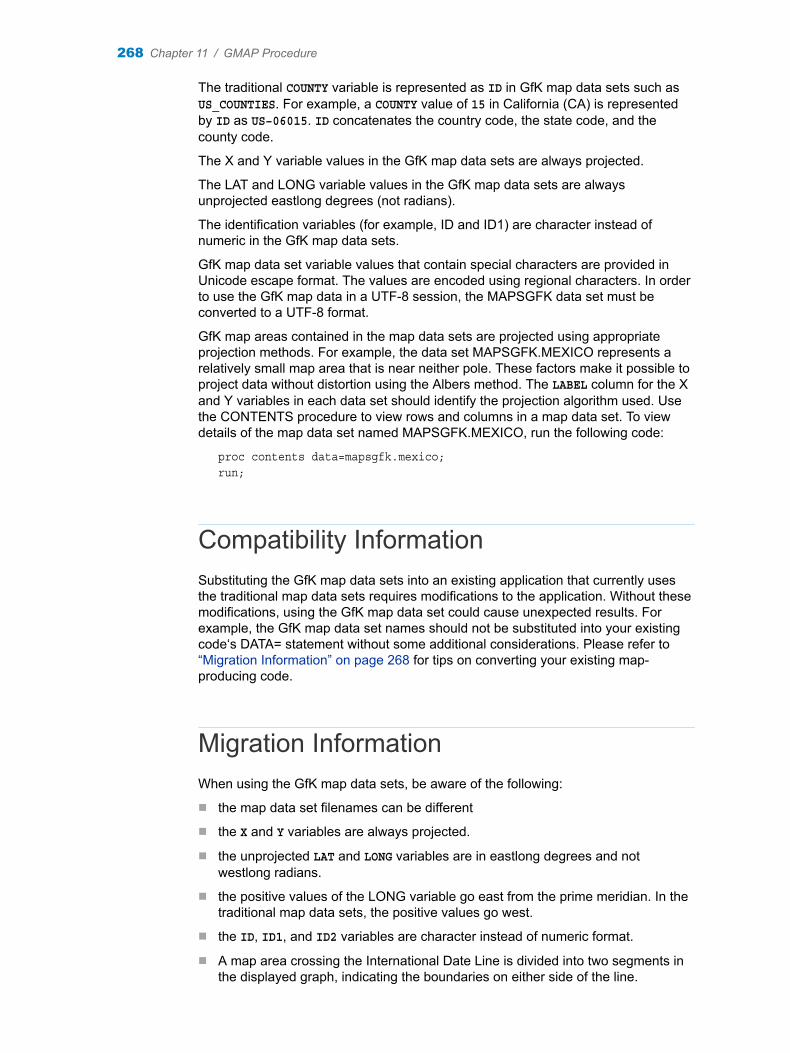
The traditional COUNTY variable is represented as ID in GfK map data sets such as US_COUNTIES. For example, a COUNTY value of 15 in California (CA) is represented by ID as US–06015. ID concatenates the country code, the state code, and the county code.
The X and Y variable values in the GfK map data sets are always projected.
The LAT and LONG variable values in the GfK map data sets are always unprojected eastlong degrees (not radians).
The identification variables (for example, ID and ID1) are character instead of numeric in the GfK map data sets.
GfK map data set variable values that contain special characters are provided in Unicode escape format. The values are encoded using regional characters. In order to use the GfK map data in a UTF-8 session, the MAPSGFK data set must be converted to a UTF-8 format.
GfK map areas contained in the map data sets are projected using appropriate projection methods. For example, the data set MAPSGFK.MEXICO represents a relatively small map area that is near neither pole. These factors make it possible to project data without distortion using the Albers method. The LABEL column for the X and Y variables in each data set should identify the projection algorithm used. Use the CONTENTS procedure to view rows and columns in a map data set. To view details of the map data set named MAPSGFK.MEXICO, run the following code:
proc contents data=mapsgfk.mexico;run;
Compatibility InformationSubstituting the GfK map data sets into an existing application that currently uses the traditional map data sets requires modifications to the application. Without these modifications, using the GfK map data set could cause unexpected results. For example, the GfK map data set names should not be substituted into your existing code‘s DATA= statement without some additional considerations. Please refer to “Migration Information” on page 268 for tips on converting your existing map-producing code.
Migration InformationWhen using the GfK map data sets, be aware of the following:
n the map data set filenames can be different
n the X and Y variables are always projected.
n the unprojected LAT and LONG variables are in eastlong degrees and not westlong radians.
n the positive values of the LONG variable go east from the prime meridian. In the traditional map data sets, the positive values go west.
n the ID, ID1, and ID2 variables are character instead of numeric format.
n A map area crossing the International Date Line is divided into two segments in the displayed graph, indicating the boundaries on either side of the line.
268 Chapter 11 / GMAP Procedure

Examples of affected regions are Russia, Tonga, and territories and islands in the Pacific ocean.
Refer to “Reworking Code That Uses Traditional Map Data Sets” on page 350 for information and tips.
The METAMAPS Data SetThe maps data set library that is referenced by both the MAPS and MAPSSAS librefs have a data set named METAMAPS. This data set contains metadata about all of the data sets that are delivered in the library. MEMNAME is just one of the variables to find among the metadata in MAPS.METAMAPS and MAPSSAS.METAMAPS:
Note: GfK GeoMarketing GmbH does not include a comparable data set in its MAPSGFK library that SAS has licensed.
VariableDescription
VARxidentifies the name of the variable in the data set, where x is a numerical value.
LABELxdescribes VARx in the data set.
MEMNAMEidentifies the names of all of the data sets that are delivered in the MAPS or MAPSSAS library.
Special GfK Data Sets for Annotating MapsThere are several data sets in the MAPSGFK library that enable you to easily add labels or markers to the maps. Some of their names differ from any traditional data sets that you might have used. Though the non-map data sets contain coordinates for map features such as cities, they cannot be used as map data sets.
The X and Y variables containing projected coordinates in the USCENTER, USCENTER_ALL, USCITY, and USCITY_ALL data sets can be used directly with the map data sets specified in the file header. If you want to use a different map data set, then use the LAT and LONG variables provided in the MAPSGFK data set. Use the Chapter 12, “GPROJECT Procedure,” on page 433 to project them using the map data set projection parameters.
MAPSGFK.USCENTER_ALLcontains the coordinates of the visual center of each state in the U.S. and Washington, D.C., Puerto Rico, and the U.S. Virgin Islands. It also contains coordinates in the ocean for states that are too small to contain a label. There are two pairs of variables for locating labels using Annotate data sets. The X and Y variables contain projected coordinates and can be used with the MAPSGFK.US_ALL data set. The LONG and LAT variables contain the unprojected longitude and latitude in degrees (not radians). These can be used
Concepts: GMAP Procedure 269

to place labels on any US data set, noting that you can subset the data set by state as needed.
MAPSGFK.USCENTERis similar to USCENTER_ALL, except that it does not include Puerto Rico and the U.S. Virgin Islands. The X and Y variables contain projected coordinates and can be used with the MAPSGFK.US data set.
MAPSGFK.USCITY_ALLcontains the locations of selected cities in the U.S. Many city names occur in more than one state, so you might have to subset by state to avoid duplication. There are two pairs of variables for locating labels using Annotate data sets. The X and Y variables contain projected coordinates using the Miller II projection method. These variables can be used with the MAPSGFK.US_ALL data set. The LONG and LAT variables contain the unprojected longitude and latitude in degrees (not radians). These can be used to place labels on any US data set, noting that you can subset the data set by state as needed.
MAPSGFK.USCITYis similar to USCITY_ALL, except that it does not include Puerto Rico and the U.S. Virgin Islands. The X and Y variables contain projected coordinates using the Albers projection method. These variables can be used with the MAPSGFK.US data set.
Duplicate observations can be listed in the output data set. This occurs because the map data set includes towns, villages, hamlets, and other non-city areas that can share the same name with a city.
MAPSGFK.US_COUNTIEScontains a projected US county map with Alaska and Hawaii in physical locations. Puerto Rico is not included. Many county names occur in more than one state, so you might have to subset by state to avoid duplication. The LONG and LAT variables contain the unprojected longitude and latitude in degrees (not radians). These can be used to place labels on any US data set, noting that you can subset the data set by state as needed.
MAPSGFK.US_STATEScontains a projected US state map with Alaska and Hawaii in physical locations. Puerto Rico is not included. The LONG and LAT variables contain the unprojected longitude and latitude in degrees (not radians). These can be used to place labels on any US data set, noting that you can subset the data set by state as needed.
MAPSGFK.UScontains a projected US state map with Alaska and Hawaii inset into the map. Puerto Rico is not included. The LONG and LAT variables are not included.
MAPSGFK.US_ALLcontains a projected US county map with Alaska and Hawaii in physical locations. Puerto Rico and the United States Virgin Islands are included. Many county names occur in more than one state, so you might have to subset by state to avoid duplication. The LONG and LAT variables contain the unprojected longitude and latitude in degrees (not radians). These can be used to place labels on any US data set, noting that you can subset the data set by state as needed.
MAPSGFK.WORLD_CITIEScontains the location of more than 200,000 international cities. Many city names occur more than once, so you might want to specify a country, state, province, or region variable to differentiate the cities. This data set does contain local city spellings. The CITY variable has mixed case values. The CITY2 variable values
270 Chapter 11 / GMAP Procedure

in this data set are normalized. This means that they are uppercase and stripped of all spaces and characters that are not alphabetic or numeric. This CITY2 variable is used by the GEOCODE procedure. The X and Y variables contain projected coordinates. The LONG and LAT variables contain the unprojected longitude and latitude in degrees (not radians). These can be used to place annotation labels on any international data set.
Note:
MAPSGFK.WORLD_CITIES_ALL is an alternate data set that contains the location of more than a million cities worldwide. It contains the same variables as the MAPSGFK.WORLD_CITIES data set. The more comprehensive data set is available for download from the SAS Maps and Geocodng website. You are required to access the website with your SAS profile. You might be required to enter your site information. This unabridged data set is updated annually.
Special Traditional Data Sets for Annotating MapsThere are several data sets in the MAPSSAS library that enable you to easily label maps. These data sets contain coordinates for map features such as cities, but cannot be used as map data sets.
MAPS.USCENTERcontains the coordinates of the visual center of each state in the U.S. and Washington, D.C.. It also contains coordinates in the ocean for states that are too small to contain a label. There are two pairs of variables for locating labels using Annotate data sets. The X and Y variables are projected and can be used with the MAPS.US and MAPS.USCOUNTY data sets. The LONG and LAT variables are unprojected longitude and latitude in radians and can be used with the MAPS.STATES, MAPS.COUNTIES, and MAPS.COUNTY data sets.
MAPS.USCITYcontains the locations of selected cities in the U.S. Many city names occur in more than one state, so you might have to subset by state to avoid duplication. There are two pairs of variables for locating labels using Annotate data sets. The X and Y variables contain projected coordinates and can be used with the MAPS.US and MAPS.USCOUNTY data sets. The LONG and LAT variables contain the unprojected longitude and latitude in radians. These can be used to place labels on the MAPS.STATES, MAPS.COUNTIES, or MAPS.COUNTY data sets.
Duplicate observations can be listed in the output data set. This occurs because the map data set includes towns, villages, hamlets, and other non-city areas that can share the same name with a city. Differentiate the output with the FEATYPE variable, which contains the area type.
For details about each of these data sets, see the MAPS.METAMAPS data set or the MAPSSAS.METAMAPS data set.
Concepts: GMAP Procedure 271

About Response Data Sets
Definition: Response Data SetA response data set is a SAS data set that can contain other variables, but requires the following variables:
n one or more response variables that contain data values that are associated with map areas. Each value of the response variable is associated with a map area in the map data set.
n identification variables that identify the map area to which a response value belongs. These variables must be the same as those that are contained in the map data set.
Using the Response Data Set with the Map Data SetsThe map data set and the response data set must be used independently in the PROC GMAP statement. The response data set is specified by the DATA= option and the map data set is specified by the MAP= option. The values of the map area id-variables in the response data set determine the map areas to be included on the map. Unless the ALL option is used in the PROC GMAP statement, only the map areas with response values are shown on the map. As a result, you do not need to subset your map data set if you are mapping only a small section of the map. However, if you map the same small section frequently, then create a subset of the map data set for efficiency.
If you have a response data set named SASHELP.US_DATA, then the syntax for using the GMAP procedure might resemble the following:
proc gmap map=mapsgfk.us data=sashelp.us_data; id state; choro region;run;quit;
SAS provides sample response data sets in the SASHELP library. These data sets are available for you to use for examples and for testing code. Some of the examples in this chapter use sample response data sets such as SASHELP.US_DATA and SASHELP.DEMOGRAPHICS.
272 Chapter 11 / GMAP Procedure

About Response VariablesThe GMAP procedure can produce block, choropleth, prism, and surface maps for both numeric and character response variables. Numeric variables fall into two categories: discrete and continuous.
n Discrete variables contain a finite number of specific numeric values that are to be represented on the map. For example, a variable that contains only the values 1989 or 1990 is a discrete variable.
n Continuous variables contain a range of numeric values that are to be represented on the map. For example, a variable that contains any real value between 0 and 100 is a continuous variable.
Numeric response variables are treated as continuous variables unless the DISCRETE option is used in the action statement.
About Response LevelsResponse levels are the values that identify categories of data on the graph. The categories that are shown on the graph are based on the values of the response variable. Based on the type of the response variable, a response level can be determined by any of the following:
n a character value
n the MIDPOINTS= option
n a range of numeric values
n a specific numeric value
When response levels are determined by a character value, the GMAP procedure treats each unique value as a response level. For example, if the response variable contains the names of ten regions, each region is a response level, resulting in ten response levels.
When character response levels are determined by the MIDPOINTS= option, any response variable values that do not match one of the specified response level values are ignored.
When response levels are determined by a range of numeric values, each response level has a similar number of observations. These options are exceptions to this:
n The LEVELS= option specifies the number of response levels to be graphed for the response variable. The LEVELS=number-of-midpoints option is ignored if either the DISCRETE or MIDPOINTS= option is used.
n The DISCRETE option causes the numeric variable to be treated as a discrete variable.
n The MIDPOINTS= option chooses specific response level values as medians of the value ranges.
If the response variable values are continuous, then the GMAP procedure assigns response level intervals automatically unless you specify otherwise. The response levels represent a range of values rather than a single value.
Concepts: GMAP Procedure 273

When response levels are determined by specific numeric values, and the DISCRETE option is specified, one level is created for each value. If the response variable has an associated format, then each formatted value is represented by a different response level.
The AREA, BLOCK, CHORO, and PRISM statements assign patterns to response levels. In CHORO and PRISM maps, response levels are shown as map areas. However, in BLOCK maps, response levels are shown as blocks. If you specify the AREA statement on a BLOCK map, then the response levels for AREA variable are shown as map areas. The default fill pattern for the response level is solid.
PATTERN statements can define the fill patterns and colors for both blocks and map areas. PATTERN definitions that define valid block patterns are applied to the blocks (response levels), and PATTERN definitions that define valid map patterns are applied to map areas.
See “PATTERN Statement” on page 78 for more information about fill pattern values and default pattern rotation.
About Identification VariablesFor map data sets and response data sets, id-variables identify the map areas (for example, counties, states, or provinces) that make up the map. A unit area or map area is a group of observations with the same ID value. The GMAP procedure matches the value of the response variables for each map area in the response data set to the corresponding map area in the map data set. It does this in order to create the display graphs.
Displaying Map Areas and Response DataWhether the GMAP procedure draws a map area and whether it displays patterns for response values depends on the contents of the response data set and on the ALL and MISSING options. The following table describes the conditions under which the procedure does or does not display map areas and response data.
Table 11.4 Displaying Map Areas and Response Data
Characteristic of the response data set Additional variables Result
Includes the map area. The map area has a response value.
The procedure draws the map area and displays the response data.
Includes the map area. The response value for the map area is a missing value.
The procedure draws the map area but leaves it empty.
Includes the map area. The response value for the map area is a missing value and the MISSING
The procedure draws the map area and displays a
274 Chapter 11 / GMAP Procedure

Characteristic of the response data set Additional variables Result
option is used in the map statement.
response level for the missing value.
Includes the map area. The map area has a response value and the MAP= option and the DATA= statement specify the same map data set.
The procedure draws the map area and displays boundary outlines but does not display the value of the response variable or variables.
Does not include the map area.
The ALL option is used in the PROC GMAP statement.
The procedure draws the map area but leaves it empty.
Does not include the map area.
The ALL option is not used.
The procedure does not draw the map area.
Summary of UseTo use the GMAP procedure, you must do the following:
1 When using a map data set, determine what processing needs to be done to the map data set before it is displayed. Use the GPROJECT, GREDUCE, and GREMOVE procedures or a DATA step to perform the necessary processing.
2 Issue a LIBNAME statement for the SAS data set that contains the response data set, or use a DATA step to create a response data set.
3 When using a map data set, use the PROC GMAP statement to identify the map data set as the MAP= value and response data set as the DATA= value.
4 Use the ID statement to specify the id-variable(s).
5 Use a BLOCK, CHORO, PRISM, or SURFACE statement to identify the response variable and generate the map.
Accessing SAS Maps and Geocoding Resources Online
Visit SAS Maps and Geocoding online to download data updates, sample SAS/GRAPH programs that use the production-level map data sets delivered with SAS/GRAPH, and GIF images of maps. You are required to access the website with your SAS profile. You might be required to enter your site information. SAS Maps
Concepts: GMAP Procedure 275

and Geocoding is located at the following URL: https://support.sas.com/en/knowledge-base/maps-geocoding.html
After downloading and unzipping map data sets, you must take them out of transport format by running the CIMPORT procedure using your current version of SAS. For more information, see the “CIMPORT Procedure” in Base SAS Procedures Guide.
Importing Maps from Esri ShapefilesStarting with SAS 9.4M5, you can import Esri shapefiles as map data sets by using the Base SAS MAPIMPORT procedure. Prior to SAS SAS 9.4M5, this procedure is part of SAS/GRAPH, and you must have SAS/GRAPH installed to use it. Depending on the type of coordinates that are in your shapefile, you might want to perform additional processing. In SAS 9.4M6 and later releases, for example, you might want to project the map with the Base SAS GPROJECT procedure, or use the Base SAS GREDUCE procedure to create a DENSITY variable for reducing your data. Prior to SAS 9.4M6, the GPROJECT procedure and the GREDUCE procedure were part of SAS/GRAPH, and you had to have SAS/GRAPH installed to use either of them.
For more information, see Chapter 15, “MAPIMPORT Procedure,” on page 503.
Syntax: GMAP ProcedureRestrictions: This procedure cannot use input data that has been processed in CAS. The input data
must be in sequential order. Because CAS is a distributed system, sequential order of data in CAS cannot be guaranteed.A SAS LASR Analytic server should not be used as the repository for map data sets. Essential data sequencing is lost as the data is distributed amongst this server’s nodes.
Requirement: n An input map data set is required. If not specified, an input map data set must have been created before issuing the PROC GMAP statement.
n A response data set is required. If not specified, a response data set must have been created before issuing the PROC GMAP statement.
n One ID statementn At least one CHORO, BLOCK, PRISM, or SURFACE statement
Supported Statements:
TITLE, FOOTNOTE, NOTE, LEGEND, PATTERN, GOPTIONS
Supports: RUN-group processing
Note: The procedure can include the SAS/GRAPH statements BY on page 49 and NOTE on page 93, as well as the Base SAS statements FORMAT, LABEL, and WHERE. See “Overview of Global Statements” on page 47 and SAS DATA Step Statements: Reference for more information.
PROC GMAP MAP=map-data-setDATA=response-data-set<ALL>
276 Chapter 11 / GMAP Procedure

<ANNOTATE=Annotate-data-set><DENSITY=0 ...6 | LOW | MEDIUM | HIGH><GOUT=<libref.>output-catalog><IMAGEMAP=output-data-set><LATLON><RESOLUTION=1 ...10 | AUTO | NONE><STRETCH><UNIFORM>;
ID id-variable(s);AREA response-variable </ options>;BLOCK response-variable(s) </ options>;CHORO response-variable(s) </ options>;PRISM response-variable(s) </ options>;SURFACE response-variable(s) </ options>;
PROC GMAP StatementIdentifies the map data set and the response data set that contain the variables associated with the map. The statement also provides the option to display all map areas and to specify annotation and an output catalog.
Requirement: Both a map data set and a response data set are required.
SyntaxPROC GMAP MAP=map-data-setDATA=response-data-set<ALL><ANNOTATE=Annotate-data-set><DENSITY=0 ...6 | LOW | MEDIUM | HIGH><GOUT=<libref.>output-catalog><IMAGEMAP=output-data-set><LATLON><RESOLUTION=1 ...10 | AUTO | NONE><STRETCH><UNIFORM>;
Summary of Optional ArgumentsALL
specifies that the maps generated by the procedure should include all of the map areas from the map data set. This occurs even if the response data set does not include an observation for the map area.
ANNOTATE=Annotate-data-setspecifies a data set to annotate all of the maps that are produced by the GMAP procedure.
PROC GMAP Statement 277

DENSITY=0 – 6 | LOW | MEDIUM | HIGHfor maps that have a DENSITY variable, specifies the density of map observations that are used.
GOUT=<libref.>output-catalogspecifies the SAS catalog in which to save the graphics output that is produced by the GMAP procedure for later replay.
IMAGEMAP=output-data-setcreates a temporary SAS data set that is used to generate an image map.
LATLONspecifies that the LAT and LONG variables from the map data set are used for coordinate data instead of the Y and X variables.
RESOLUTION=1 – 10 | AUTO | NONEfor maps that have a RESOLUTION variable, specifies the resolution level of map observations that are used.
STRETCHstretches map extents to cover all available space in the device. This might cause the map to be distorted.
UNIFORMcauses the same legend and coloring to be used for all maps produced by the procedure instead of being calculated within each BY group for each map.
Required ArgumentsDATA=response-data-set
identifies the SAS data set that contains the response values or the response values and the spatial information that are evaluated and represented on the map. If not specified, a response data set must have been created before issuing the PROC GMAP statement.
Default The GMAP procedure uses the most recently created SAS data set.
Requirements This statement is required if no response data set was created before issuing the PROC GMAP statement.
A response data set must contain the same identification variable or variables as the specified map data set, along with the values of the response variable.
See “The SAS Data Set: Your Key to the SAS System” in Step-by-Step Programming with Base SAS
“About Data Set Options” in SAS Data Set Options: Reference
MAP=map-data-setnames a map data set that contains either the X and Y or LAT and LONG coordinates, or all, for the boundary points of each map area. This includes map data sets licensed by SAS from GfK GeoMarketing GmBH and converted by SAS to a SAS data set format.
Requirement This statement is required.
Interaction The map data set must contain the same identification variable or variables as the response data set being used.
278 Chapter 11 / GMAP Procedure

See “About Map Data Sets” on page 255
Optional ArgumentsPROC GMAP statement options affect all of the graphs that are produced by the procedure.
ALLspecifies that the maps generated by the procedure should include all of the map areas from the map data set. This occurs even if the response data set does not include an observation for the map area. When you use the ALL option and a BY statement in a RUN group, the maps generated for each BY group include every map area from the map data set.
See “Displaying Map Areas and Response Data” on page 274
ANNOTATE=Annotate-data-setspecifies a data set to annotate all of the maps that are produced by the GMAP procedure. To annotate individual maps, use the ANNOTATE= option in the action statement.
Alias ANNO=
See “Overview: The Annotate Facility” in SAS/GRAPH: Reference
DENSITY=0 – 6 | LOW | MEDIUM | HIGHfor maps that have a DENSITY variable, specifies the density of map observations that are used. The value that you specify indicates the maximum value that the DENSITY variable can have for the observation to be displayed. For example, if you specify DENSITY=5, then only observations in the map data set whose DENSITY value is less than or equal to 5 are displayed.
Intuitively, the DENSITY variable specifies how close a map point is to other map points. If there are many map points in close proximity (high density), then it is possible to eliminate a number of them without seriously degrading the quality of the map. Many map data sets supplied by SAS contain a DENSITY variable. For map data sets that do not contain a DENSITY variable, you can add and populate the variable using the GREDUCE procedure.
You can specify an integer from 0 to 6 for the DENSITY option, or you can specify one of the descriptors. LOW is equivalent to DENSITY= 1. MEDIUM is equivalent to DENSITY= 3, HIGH is equivalent to DENSITY= 6.
If you do not specify the DENSITY= option, nor a RESOLUTION= option, then this is the same as specifying RESOLUTION= AUTO. All of the observations in a map data set are displayed that correspond to the resolution that the device displaying the map is using. This is regardless of whether the input map data set contains a DENSITY variable or not.
Alias L | MED | M | HI | H
Default DENSITY=6
Restriction If the map data set does not contain a column of DENSITY values, then a warning is issued and the option is ignored.
Interactions When the DENSITY= option is specified, and the RESOLUTION= option is not, the DENSITY= option is used. If the DENSITY= option is not specified, then the RESOLUTION= option is used
PROC GMAP Statement 279

automatically, regardless of whether it is actually specified. If specified, the RESOLUTION= setting is used. Otherwise, the RESOLUTION= value is set to the numeric level corresponding to the resolution that the device displaying the map is using.
If you specify both the RESOLUTION= and DENSITY= options, and those variables exist in the input map data set, then the RESOLUTION= option takes precedence.
Tip Specifying DENSITY=0 yields a different result than running your code with the DENSITY= option removed.
See Chapter 13, “GREDUCE Procedure,” on page 471 for information about the DENSITY variable.
“RESOLUTION=1 – 10 | AUTO | NONE” on page 281
Example “Example 15: Using GfK GeoMarketing Map Data to Produce a Simple Prism Map” on page 391
GOUT=<libref.>output-catalogspecifies the SAS catalog in which to save the graphics output that is produced by the GMAP procedure for later replay. You can use the GREPLAY procedure to view the graphs stored in the catalog. If you do not use the GOUT= option, catalog entries are written to the default catalog WORK.GSEG, which is erased at the end of your session.
Restriction Not supported by ActiveX
See “Specifying the Catalog Name and Entry Name for Your GRSEGs ” in SAS/GRAPH: Reference
IMAGEMAP=output-data-setcreates a temporary SAS data set that is used to generate an image map in an SVG file when you are sending output to the LISTING destination. (This option is not necessary when you are sending output to the HTML destination.) The drill-down URLs in the image map must be provided by variables in the input data set. These variables are identified to the procedure with the HTML= and HTML_LEGEND= options.
See “Adding Links and Enhancements with the URL=, HTML=, and HTML_LEGEND= Options” in SAS/GRAPH: Reference and “Enhancing Drill-Down Behavior in SVG Presentations Using HTML Attributes” in SAS/GRAPH: Reference
LATLONspecifies that the LAT and LONG variables from the map data set are used for coordinate data instead of the Y and X variables. The LAT and LONG variables represent the latitude and longitude coordinates, respectively. All GfK GeoMarketing and most traditional map data sets contain both sets of variables (Y, X, and LAT, LONG) for projected and unprojected maps. By default, the Y and X variables are used to produce a projected map. However, when LATLON is specified, the Y and X variables are no longer required by the GMAP procedure.
Alias LATLONG
Example “Example 4: Projecting an Annotate Data Set” on page 465
280 Chapter 11 / GMAP Procedure
RESOLUTION=1 – 10 | AUTO | NONEfor maps that have a RESOLUTION variable, specifies the resolution level of map observations that are used. The numeric value that you specify indicates the maximum value that the RESOLUTION variable can have for the observation to be displayed. For example, if you specify RESOLUTION=5, then only observations in the map data set whose RESOLUTION value is less than or equal to 5 are displayed.
The RESOLUTION variable specifies the screen resolution at which to display a map point. If there are many map points in close proximity (high density), then it is possible to eliminate a number of them without seriously degrading the quality of the map. Many map data sets supplied by SAS contain a RESOLUTION variable.
You can specify an integer from 1 to 10 for the RESOLUTION option, or you can specify AUTO or NONE. The integer correlates to the number of pixels displayed on the map. A low resolution value indicates that a smaller number of pixels is displayed. For example, a RESOLUTION value of 4 equates to 800 x 600 pixels displayed. Specifying AUTO defaults to the resolution setting of the device being used in the GMAP procedure. A RESOLUTION set to NONE indicates that the DENSITY option, if specified, is used instead.
If you do not specify the RESOLUTION= option, nor a DENSITY= option, then this is the same as specifying RESOLUTION= AUTO. All of the observations in a map data set are displayed that correspond to the resolution that the device displaying the map is using. This is regardless of whether the input map data set contains a RESOLUTION variable or not.
Alias RES=
Default RESOLUTION=AUTO when the DENSITY option is not specified. When the DENSITY option is specified, RESOLUTION=NONE.
Restriction If the map data set does not contain a column of RESOLUTION values, then a warning is issued and the option is ignored.
Interactions When the DENSITY= option is specified, and the RESOLUTION= option is not, the DENSITY= option is used. If the DENSITY= option is not specified, then the RESOLUTION= option is used automatically, regardless of whether it is actually specified. The RESOLUTION= value is set to the level corresponding to the resolution that the device displaying the map is using.
If you specify both the RESOLUTION= and DENSITY= options, and those variables exist in the input map data set, then the RESOLUTION= option is used. In this case the DENSITY= option is ignored.
See Table 11.24 on page 267 for the correlation between the RESOLUTION value and the number of pixels displayed.
Example “Example 1: Using GfK GeoMarketing Map Data to Produce a Simple Block Map” on page 353
STRETCHstretches map extents to cover all available space in the device. This might cause the map to be distorted. When this option is applied to the PROC GMAP statement, it applies to all statements. If applied to a single statement, it applies only to that statement.
PROC GMAP Statement 281

Restriction Not supported by ActiveX.
UNIFORMcauses the same legend and coloring to be used for all maps produced by the procedure instead of being calculated within each BY group for each map. The UNIFORM option pre-scans the data to generate a categorization across all the data, regardless of BY grouping, and applies that categorization to all maps in the BY group. This results in all maps uniformly displaying legends and coloring such that a single value always has the same color in multiple maps.
When specified in a PROC GMAP statement, UNIFORM applies to all BLOCK, CHORO, AREA, and PRISM statements included within the GMAP run-group.
When omitted from the PROC GMAP statement, and specified on an individual BLOCK, AREA, CHORO, or PRISM statement, UNIFORM applies only to the maps produced by that statement.
ID StatementIdentifies the variable or variables in the input data set(s) that define map areas.
Requirement: At least one id-variable is required.
SyntaxID id-variable(s);
Required Argumentid-variable(s)
identifies one or more variables in the map and response data sets that define a map area. This argument is used only when map and response data sets are specified.
Every variable that is listed in the ID statement must appear in both the map and response data sets. The variable identified by the id-variable(s) argument can be of type numeric or character and should have the same name, type, and length in both the response and map data sets.
Note: If the id-variables in the response data set and map data set do not have the same length, then your map areas might not be drawn correctly.
See “About Identification Variables” on page 274
Examples “Example 1: Using GfK GeoMarketing Map Data to Produce a Simple Block Map” on page 353
“Example 5: Using GfK GeoMarketing Map Data to Assign a Format to the Response Variable” on page 363
282 Chapter 11 / GMAP Procedure

“Example 9: Using GfK GeoMarketing Map Data to Produce a Simple Choropleth Map” on page 374
AREA Statementapplies color to the regions in BLOCK and PRISM maps based on values of a specified response variable.
Requirement: The response variable is required. The AREA statement must be used in conjunction with either a BLOCK or PRISM statement.
SyntaxAREA response-variable </ options>;
Summary of Optional ArgumentsDISCRETE
generates a separate response level (color and surface pattern) for each different value of the formatted response variable.
LEGEND=LEGEND<1 …99>specifies the LEGEND statement to associate with the map.
LEVELS=number-of-response-levels | ALLspecifies the number of response levels to be graphed for the response variable.
MIDPOINTS=value-list | OLDspecifies the response levels for the range of response values that are represented by each level (pattern and color combination).
MISSINGaccepts a missing value as a valid level for the response variable.
NOLEGENDsuppresses the legend.
PERCENTcauses GMAP to collect all response values (or their statistic) and chart each region as a percentage of the whole.
RANGEcauses GMAP to display, in the legend, the starting value and ending value of the range around each midpoint specified with the MIDPOINTS= option (instead of displaying just the midpoints).
STATFMT=format-specificationoverrides the GMAP default format for percent of PERCENT8.2.
STATISTIC=FIRST | SUM | FREQUENCY | MEANspecifies the statistic for GMAP to chart.
UNIFORM
AREA Statement 283

causes the same legend and coloring to be used for all maps produced by the procedure instead of being calculated within each BY group for each map.
Required Argumentresponse-variable
specifies the variable in the response data set. Areas that correspond to response variables with missing values are not colored unless you use the MISSING option in the AREA statement. This variable is represented in all BLOCK and PRISM maps in the same RUN group.
See “About Response Variables” on page 273
Optional ArgumentsOptions in an AREA statement affect all of the maps that are produced by that statement. You can specify as many options as you want and list them in any order. All of these options are the same as the normal GMAP options except that they apply to the areas of regions only, and not to the bar heights.
DISCRETEgenerates a separate response level (color and surface pattern) for each different value of the formatted response variable.
The LEVELS=number of midpoints option is ignored when you use the DISCRETE option.
If you specify the DISCRETE option, then distinct, non-continuous colors are used for the response values. If you specify the LEVELS= option instead, then a color ramp is used to assign each response value a continuous color scheme.
Note If the data does not contain a value in a particular range of the format, that formatted range is not displayed in the legend.
LEGEND=LEGEND<1 …99>specifies the LEGEND statement to associate with the map. The LEGEND= option is ignored if the specified LEGEND definition is not currently in effect. In the GMAP procedure, the BLOCK statement produces a legend unless you use the NOLEGEND option. If you use the SHAPE= option in a LEGEND statement, only the value BAR is valid. Most of the LEGEND options described in “LEGEND Statement” on page 56 are supported by ActiveX. If a LEGEND option is not supported by ActiveX, it is noted in the LEGEND option definition.
Restriction Partially supported by ActiveX
See “LEGEND Statement” on page 56.
LEVELS=number-of-response-levels | ALLspecifies the number of response levels to be graphed for the response variable.
Use LEVELS= to specify the number of response variables when the response variables are numeric. When you specify LEVELS=ALL, all unique numeric or character response variable values are graphed.
284 Chapter 11 / GMAP Procedure

Each response level is assigned a different surface pattern and color combination. The prism and block heights are based on the data value of the corresponding response variable.
If you specify the LEVELS= option, then a color ramp is used to assign each response value a continuous color scheme. The response values are assigned lighter and darker values of a color scheme to express lower and higher response values. If you specify the DISCRETE option, then distinct, non-continuous colors are used for the response values.
If neither the LEVELS= option nor the DISCRETE option is used, then the GMAP procedure determines the number of response levels by using the formula FLOOR(1+3.3 log(n)), where n is the number of response variable values.
The LEVELS=number-of-response-levels option is ignored when you use the DISCRETE or MIDPOINTS=value-list option. It is also ignored when the response variables are character. When MIDPOINTS=OLD is used with the LEVELS= option, default midpoints are generated using the Nelder algorithm (Applied Statistics 25:94–7, 1976).
Default An equal-distribution (quantizing) algorithm is used to determine each level.
Example Here is an example that produces a block map where there are five levels categorized for the blocks.:BLOCK ELECT / LEVELS=5;AREA CANDIDATE / DISCRETE NOLEGEND;
Regions under the blocks are colored by DISCRETE CANDIDATE. No legend is shown for the CANDIDATE values, but a legend is shown for the ELECT values.
MIDPOINTS=value-list | OLDspecifies the response levels for the range of response values that are represented by each level (pattern and color combination).
For numeric response variables, value-list is either an explicit list of values or a starting value and an ending value with an interval increment, or a combination of both forms:
n n < ...n>
n n TO n <BY increment>
n n < ...n > TO n <BY increment> <n< ...n>>
By default, the increment value is 1. You can specify discrete numeric values in any order. In all forms, n can be separated by blanks or commas. An example is: midpoints=(2 4 6) midpoints=(2,4,6) midpoints=(2 to 10 by 2)
If a numeric variable has an associated format, the specified values must be the unformatted values.
For character response variables, value-list is a list of unique character values enclosed in quotation marks and separated by blanks:
n 'value-1' < ...'value-n'> midpoints="Midwest" "Northeast" "Northwest"
Specify the values in any order. If a character variable has an associated format, the specified values must be the formatted values.
You can selectively exclude some response variable values from the map, as shown here: midpoints="Midwest"
AREA Statement 285

Only those observations for which the response variable exactly matches one of the values listed in the MIDPOINTS= option are shown on the map. As a result, observations might be excluded inadvertently if values in the list are misspelled or if the case does not match exactly.
Specifying MIDPOINTS=OLD generates default midpoints using the Nelder algorithm (Applied Statistics 25:94–7, 1976).
See The RANGE option
MISSINGaccepts a missing value as a valid level for the response variable.
NOLEGENDsuppresses the legend.
PERCENTcauses GMAP to collect all response values (or their statistic) and chart each region as a percentage of the whole. You can use the STATISTICS= option to change how the percentage is calculated—whether as a percentage of the SUM, FREQUENCY, or MEAN. If you do not use the STATISTICS= option, then STATISTICS=FIRST is assumed and the response variable of only the first observation of each region is counted. If the response variable is a text field, then STATISTIC=FREQUENCY is used, even if you specify a different value for the STATISTIC= option.
Alias PERCENTAGE
See The “STATFMT=format-specification” on page 286, and the “STATISTIC=FIRST | SUM | FREQUENCY | MEAN” on page 286.
RANGEcauses GMAP to display, in the legend, the starting value and ending value of the range around each midpoint specified with the MIDPOINTS= option (instead of displaying just the midpoints). For example, if MIDPOINTS=15 25 35, then the legend could show 10-20, 20-30, 30-40.
Restrictions The MIDPOINTS= option must be specified for the RANGE option to have any effect.
Not supported by ActiveX.
STATFMT=format-specificationoverrides the GMAP default format for percent of PERCENT8.2. Use this format when using calculated values. The STATFMT option is typically used when the STATISTIC=FREQUENCY option or the PERCENT option is used.
Alias SFMT=, SFORMAT=, STATFORMAT=
STATISTIC=FIRST | SUM | FREQUENCY | MEANspecifies the statistic for GMAP to chart. For nonnumeric variables, FREQUENCY is the only allowed value—any other value is changed to FREQUENCY and a warning is issued. The frequency of a variable does not include missing values unless the MISSING option is specified.
FIRSTGMAP matches the first observation from the DATA= data set and charts the response value from this observation only. This is the default. If more rows exist that are not processed, a warning is issued to the log.
286 Chapter 11 / GMAP Procedure

SUMAll observations matching a given ID value are added together and the summed value is charted.
FREQUENCYA count of all rows with nonmissing values is charted unless you specify the MISSING option.
MEANAll observations matching a given ID value are added together and then divided by the number of nonmissing observations matched. This value is then charted unless you specify the MISSING option.
Alias STAT=
UNIFORMcauses the same legend and coloring to be used for all maps produced by the procedure instead of being calculated within each BY group for each map. The UNIFORM option prescans the data to generate a categorization across all the data, regardless of BY grouping, and applies that categorization to all maps in the BY group. This results in all maps uniformly displaying legends and coloring such that a single value always has the same color in multiple maps.
When specified in a PROC GMAP statement, the UNIFORM option applies to all AREA, BLOCK, CHORO, and PRISM statements included within the GMAP run-group.
When omitted from the PROC GMAP statement, and specified on an individual AREA, BLOCK, CHORO, or PRISM statement, the UNIFORM option applies only to the maps produced by that statement.
Details
DescriptionIn the case of BLOCK: whereas the BLOCK statement controls the color and appearance of the blocks, the AREA statement controls the color and appearance of the regions under the block.
In the case of PRISM: whereas the PRISM statement controls the height of the prism, the AREA statement controls the color of the region. If you specify an AREA statement, the PRISM statement controls both the color and height.
BLOCK StatementCreates three-dimensional block maps on which levels of magnitude of the specified response variables are represented by blocks (bars) of varying height, pattern, and color.
Requirement: At least one response variable is required. The ID statement must be used in conjunction with the BLOCK statement.
Supported Statements:
FOOTNOTE , LEGEND, PATTERN, TITLE,
BLOCK Statement 287

SyntaxBLOCK response-variable(s) </ options>;
Summary of Optional ArgumentsAppearance options
ANNOTATE=Annotate-data-setspecifies a data set to annotate onto maps that are produced by the BLOCK statement.
BLOCKSIZE=sizespecifies the width of the blocks.
CBLKOUT=block-outline-color | SAMEoutlines all blocks in the specified color.
CDEFAULT=empty-area-fill-colorfills empty map areas in the specified color.
CEMPTY=empty-area-outline-coloroutlines empty map areas in the specified color.
CEMPTY=empty-area-outline-coloroutlines empty map areas in the specified color.
COUTLINE=area-outline-color | SAMEoutlines non-empty map areas in the specified color.
COUTLINE=area-outline-color | SAMEoutlines non-empty map areas in the specified color.
SHAPE=3D-block-shapespecifies the shape of the blocks.
STRETCHstretches map extents to cover all available space in the device.
UNIFORMcauses the same legend and coloring to be used for all maps produced by the procedure instead of being calculated within each BY group for each map.
WOUTLINE=block-outline-widthspecifies the width, in pixels, of the outline for all outlined blocks and for the outline of the map areas.
XSIZE=map-width <units>YSIZE=map-height <units>
specify the physical dimensions of the map to be drawn.XVIEW=xYVIEW=yZVIEW=z
specify coordinates of the viewing position in the reference coordinate system.
Description optionsDESCRIPTION="description"
specifies a description of the output.NAME="name"
288 Chapter 11 / GMAP Procedure

specifies the name of the GRSEG catalog entry and the name of the graphics output file, if one is created.
Legend optionsCTEXT=text-color
specifies a color for the text in the legend.LEGEND=LEGEND<1 …99>
specifies the LEGEND statement to associate with the map.NOLEGEND
suppresses the legend.
Mapping optionsAREA=n | column-name
specifies that a different map pattern be used for the surface of each map area or group of map areas on the map.
DISCRETEgenerates a separate response level (color and surface pattern) for each different value of the formatted response variable.
LEVELS=number-of-response-levels | ALLspecifies the number of response levels to be graphed for the response variable.
MIDPOINTS=value-list | OLDspecifies the response levels for the range of response values that are represented by each level (pattern and color combination).
MISSINGaccepts a missing value as a valid level for the response variable.
PERCENTcauses GMAP to collect all response values (or their statistic) and chart each region as a percentage of the whole.
RANGEdisplays value ranges in the legend.
RELZEROcreates bars and regions that are relative to a zero value.
STATFMT=format-specificationoverrides the GMAP default format for percent of PERCENT8.2.
STATISTIC=FIRST | SUM | FREQUENCY | MEANspecifies the statistic for GMAP to chart.
ODS optionsHTML_LEGEND=variable
identifies the variable in the input data set whose values create links or data tips or both.
HTML=variableidentifies the variable in the input data set whose values create links or data tips or both.
URL=character-variablespecifies a character variable whose values are URLs.
BLOCK Statement 289

Required Argumentresponse-variable(s)
specifies one or more variables in the response data set. Each response variable produces a separate map. All variables must be in the input data set. Multiple response variables are separated with blanks. Blocks are not drawn for the response variable with missing values unless you use the MISSING option in the BLOCK statement.
See “About Response Variables” on page 273.
Optional ArgumentsOptions in a BLOCK statement affect all of the maps that are produced by that statement. You can specify as many options as you want and list them in any order.
ANNOTATE=Annotate-data-setspecifies a data set to annotate onto maps that are produced by the BLOCK statement. Annotate coordinate systems 1, 2, 7, and 8 are not valid with block maps.
Alias ANNO=
See “Overview: The Annotate Facility” in SAS/GRAPH: Reference.
AREA=n | column-namespecifies that a different map pattern be used for the surface of each map area or group of map areas on the map.
You can specify pattern fills or colors or both with PATTERN statements that specify map and plot patterns. A separate PATTERN definition is needed for each specified area.
AREA=nThe value of n indicates which variable in the ID statement determines the groups that are distinguished by a surface pattern. By default, all map unit areas are drawn using the same surface fill pattern. If your ID statement has only one map area identification variable, then use AREA=1 to indicate that each map area surface uses a different pattern. If you have more than one variable in your ID statement, then use n to indicate the position of the variable that defines groups that share a pattern. When you use the AREA= option, the map data set should be sorted in order of the variables in the ID statement.
AREA=column-nameA column name defined in either the MAP= or DATA= data sets might be indicated with the column-name value. If the column name exists in both the MAP= and DATA= data sets, the column in the MAP= data set is used. When column-name is used, the areas are colored based on the AREA= value. Duplicate AREA= values might be assigned different patterns.
See “AREA Statement” on page 283, “PATTERN Statement” on page 78.
BLOCKSIZE=sizespecifies the width of the blocks. The unit of size is the character cell width for the selected output device. By default, BLOCKSIZE=2.
290 Chapter 11 / GMAP Procedure

Alias BS=
CBLKOUT=block-outline-color | SAMEoutlines all blocks in the specified color. The SAME value specifies that the outline color of a block, a block segment, or a legend is the same as the interior pattern color.
The default outline color is determined by the current style. If you specified the NOGSTYLE system option, then the default color is black for ActiveX and the first color in the color list for all other devices.
The CBLKOUT= option is not valid when SHAPE=CYLINDER.
Alias CBLOCK=
Note If you specify empty block patterns (VALUE=EMPTY in a PATTERN statement), you should not change the outline color from the default value, SAME, to a single color. Otherwise, all the outlines are one color and you can distinguish between empty areas only by their size.
CDEFAULT=empty-area-fill-colorfills empty map areas in the specified color. This option affects only map areas that are empty. Empty map areas are generated in block maps only when a map area is omitted from the response data set and the ALL option is included in the PROC GMAP statement.
The default is NONE, which draws the polygon empty, showing the background in the fill area of the polygon.
Alias CDEF=, DEFCLR=
See The CEMPTY option, the “ALL” on page 279 option, and “Displaying Map Areas and Response Data” on page 274
CEMPTY=empty-area-outline-coloroutlines empty map areas in the specified color. This option affects only map areas that are empty. Empty map areas are generated in block maps only when a map area is omitted from the response data set and the ALL option is included in the PROC GMAP statement.
The default outline color is the same as the default COUTLINE= color.
Alias CE=
See The option “ALL” on page 279 and “Displaying Map Areas and Response Data” on page 274.
COUTLINE=area-outline-color | SAMEoutlines non-empty map areas in the specified color. When COUTLINE=area-outline-color and DEVICE=ACTIVEX, both empty and nonempty map areas are outlined. The SAME value specifies that the outline color of a map area is the same as the interior pattern color.
The default outline color is determined by the current style. If you specified the NOGSTYLE system option, then the default color is black for ActiveX and the first color in the color list for all other devices.
Alias CO=
BLOCK Statement 291

Note If you specify empty map patterns (VALUE=EMPTY in a PATTERN statement), then you should not change the outline color from the default value SAME. Otherwise, all the outlines are one color and you cannot distinguish between the empty areas. Empty block patterns (VALUE=EMPTY in a PATTERN statement) are not supported by DEVICE=JAVA.
CTEXT=text-colorspecifies a color for the text in the legend. If you omit the CTEXT= option, a color specification is searched for in this order:
n the CTEXT= option in a GOPTIONS statement.
n the default, the text color that is specified in the current style.
n if you specify NOGSTYLE, then the default color is black for ActiveX and the first color in the color list for all other devices.
The CTEXT= color specification is overridden if you also use the COLOR= suboption of a LABEL= or VALUE= option in a LEGEND definition that is assigned to the map legend. The COLOR= suboption determines the color of the legend label or the color of the legend value descriptions, respectively.
Alias CT=
DESCRIPTION="description"specifies a description of the output. The maximum length for description is 256 characters. The description does not appear in the output. The descriptive text is shown in each of the following:
n the chart description for web output (depending on the device driver). See “Chart Descriptions for Web Presentations” in SAS/GRAPH: Reference for more information.
n the Table of Contents that is generated when you use the CONTENTS= option in an ODS HTML statement, assuming that the output is generated while the contents page is open.
n the description and the properties for the output in the Results window.
n the description and properties for the catalog entry in the Explorer.
n the Description field of the PROC GREPLAY window.
The description can include the #BYLINE, #BYVAL, and #BYVAR substitution options, which work as they do when used on TITLE, FOOTNOTE, and NOTE statements. Refer to “Substituting BY Line Values in a Text String” on page 112. The 256-character limit applies before the substitution takes place for these options. Thus, if in the SAS program the entry-description text exceeds 256 characters, it is truncated to 256 characters, and then the substitution is performed.
Alias DES=
Default BLOCK MAP OF variable-name
DISCRETEgenerates a separate response level (color and surface pattern) for each different value of the formatted response variable.
The LEVELS=number-of-response-levels option is ignored when you use the DISCRETE option.
292 Chapter 11 / GMAP Procedure

If you specify the DISCRETE option, then distinct, non-continuous colors are used for the response values. If you specify the LEVELS= option, then a color ramp is used to assign each response value a continuous color scheme.
Note If the data does not contain a value in a particular range of the format, that formatted range is not displayed in the legend.
HTML=variableidentifies the variable in the input data set whose values create links or data tips or both. The variable values are either links or data tips or both that are created in the HTML file generated by the ODS statement. The links are URLs pointing to web pages to display when the user clicks (drills down) on elements in the graph. Data tips are detailed information or data values that are displayed as pop-up text when a mouse pointer is positioned over elements in the graph.
Interaction When multiple observations exist in the input data set for one variable value, the first observation is used for the data tip. When that same input data set is used for an annotate data set, the last of the multiple observations is used for the annotation. Sort the data one way for the data tip and the opposite way for the annotation to alleviate any mismatch between the data tip and its annotation in the resulting graph.
See “Data Tips for Web Presentations” in SAS/GRAPH: Reference
“Adding Links and Enhancements with the URL=, HTML=, and HTML_LEGEND= Options” in SAS/GRAPH: Reference
HTML_LEGEND=variableidentifies the variable in the input data set whose values create links or data tips or both. Input data set variable values are either links or data tips or both that are created in the HTML file generated by the ODS statement. The links are associated with a legend value and point to the URL to display when the user clicks (drills down) on the value. Data tips are detailed information or data values that are displayed as pop-up text when a mouse pointer is positioned over values in the legend.
Restriction Not supported by ActiveX
See “Adding Links and Enhancements with the URL=, HTML=, and HTML_LEGEND= Options” in SAS/GRAPH: Reference
LEGEND=LEGEND<1 …99>specifies the LEGEND statement to associate with the map. The LEGEND= option is ignored if the specified LEGEND definition is not currently in effect. In the GMAP procedure, the BLOCK statement produces a legend unless you use the NOLEGEND option. If you use the SHAPE= option in a LEGEND statement, only the value BAR is valid. Most of the LEGEND options described in “LEGEND Statement” on page 56 are supported by ActiveX. If a LEGEND option is not supported by ActiveX, it is noted in the LEGEND option definition.
Restriction Partially supported by ActiveX
See “LEGEND Statement” on page 56
LEVELS=number-of-response-levels | ALLspecifies the number of response levels to be graphed for the response variable.
BLOCK Statement 293

If you specify LEVELS=ALL, then all unique numeric or character response variable values are graphed.
Each response level is assigned a different surface pattern and color combination. The block height is based on the data value of the corresponding response variable.
If you specify the LEVELS= option, then a color ramp is used to assign each response value a continuous color scheme. The response values are assigned lighter and darker values of a color scheme to express lower and higher response values. If you specify the DISCRETE option, then distinct, non-continuous colors are used for the response values.
If neither the LEVELS= option nor the DISCRETE option is used, then the GMAP procedure determines the number of response levels by using the formula FLOOR(1+3.3 log(n)), where n is the number of response variable values.
By default, an equal-distribution (quantizing) algorithm is used to determine each level.
The LEVELS=number-of-response-levels option is ignored when you use the DISCRETE or MIDPOINTS=value-list option. It is also ignored when the response variables are character. When MIDPOINTS=OLD is used with the LEVELS= option, default midpoints are generated using the Nelder algorithm (Applied Statistics 25:94–7, 1976).
Note If you specified the NOGSTYLE system option, then noncontinuous colors are used by default.
MIDPOINTS=value-list | OLDspecifies the response levels for the range of response values that are represented by each level (pattern and color combination).
For numeric response variables, value-list is either an explicit list of values or a starting value and an ending value with an interval increment, or a combination of both forms:
n n < ...n>
n n TO n <BY increment>
n n < ...n > TO n <BY increment> <n< ...n>>
By default, the increment value is 1. You can specify discrete numeric values in any order. In all forms, n can be separated by blanks or commas. For example: midpoints=(2 4 6) midpoints=(2,4,6) midpoints=(2 to 10 by 2)
If a numeric variable has an associated format, the specified values must be the unformatted values.
For character response variables, value-list is a list of unique character values enclosed in quotation marks and separated by blanks:
n 'value-1' < ...'value-n'> midpoints="Midwest" "Northeast" "Northwest"
Specify the values in any order. If a character variable has an associated format, the specified values must be the formatted values.
You can selectively exclude some response variable values from the map, as shown here: midpoints="Midwest"
Only those observations for which the response variable exactly matches one of the values listed in the MIDPOINTS= option are shown on the map. As a result, observations might be excluded inadvertently if values in the list are misspelled or if the case does not match exactly.
294 Chapter 11 / GMAP Procedure

Specifying MIDPOINTS=OLD generates default midpoints using the Nelder algorithm (Applied Statistics 25:94–7, 1976).
See The RANGE option
Example “Example 17: Using GfK GeoMarketing Map Data When Specifying Midpoints in a Prism Map” on page 396
MISSINGaccepts a missing value as a valid level for the response variable.
See “Displaying Map Areas and Response Data” on page 274.
NAME="name"specifies the name of the GRSEG catalog entry and the name of the graphics output file, if one is created.
The following applies to name:
n The name can be up to 256 characters in length.
n Special characters in the name are converted to underscores.
n For the GRSEG entry name:
o The name is truncated to eight characters.
o The first character is always represented in uppercase, and all other characters are represented in lowercase.
o If the name begins with a number, an underscore is prepended to the name.
o If the name duplicates an existing name, SAS/GRAPH appends a number or increments the last number used to create a unique graph name (for example, name1, name2, and so on). If necessary, the name is truncated so that the name and appended number do not exceed eight characters.
n For the graphics output filename:
o The filename is based on the NAME= value except when you use an ODS LISTING destination, a DEVICE= option, and a file reference specifying an output filename. In this case, the file reference specification overrides the NAME= value. See “Controlling Graphics Output for ODS LISTING” in SAS/GRAPH: Reference.
o All characters are represented in lowercase.
o If a number is added to the GRSEG name, the same number is added to the output filename. See “About Filename Indexing” in SAS/GRAPH: Reference.
o If the NAME= value is 8 characters or less, the filename is the GRSEG entry name.
o If the NAME= value is greater than 8 characters, the NAME= value is used as the filename. When an index number is used in the GRSEG entry name, that index number is appended to the output filename. See “About Filename Indexing” in SAS/GRAPH: Reference.
Note: If the name begins with a number, an underscore is prepended to the filename.
BLOCK Statement 295

o The maximum allowable filename length is device-specific. If the length of the name exceeds the maximum for the graphics device, an error results and no graphics output file is generated.
Default GMAP
NOLEGENDsuppresses the legend.
CEMPTY=empty-area-outline-coloroutlines empty map areas in the specified color. This option affects only map areas that are empty. Empty map areas are generated in block maps only when a map area is omitted from the response data set and the ALL option is included in the PROC GMAP statement.
The default outline color is the same as the default COUTLINE= color.
Alias CE=
See The option “ALL” on page 279 and “Displaying Map Areas and Response Data” on page 274.
COUTLINE=area-outline-color | SAMEoutlines non-empty map areas in the specified color. When COUTLINE=area-outline-color and DEVICE=ACTIVEX, both empty and nonempty map areas are outlined. The SAME value specifies that the outline color of a map area is the same as the interior pattern color.
The default outline color is determined by the current style. If you specified the NOGSTYLE system option, then the default color is black for ActiveX and the first color in the color list for all other devices.
Alias CO=
Note If you specify empty map patterns (VALUE=EMPTY in a PATTERN statement), then you should not change the outline color from the default value SAME. Otherwise, all the outlines are one color and you cannot distinguish between the empty areas.
PERCENTcauses GMAP to collect all response values (or their statistic) and chart each region as a percentage of the whole. You can use the STATISTIC= option to change how the percentage is calculated—whether as a percentage of the SUM, FREQUENCY, or MEAN. If you do not use the STATISTIC= option, then STATISTIC=FIRST is assumed and the response variable of only the first observation of each region is counted. If the response variable is a text field, then STATISTIC=FREQUENCY is used, even if you specify a different value for the STATISTIC= option.
Alias PERCENTAGE
See The “STATFMT=format-specification” on page 297, and the “STATISTIC=FIRST | SUM | FREQUENCY | MEAN” on page 297
RANGEcauses GMAP to display, in the legend, the starting value and ending value of the range around each midpoint specified with the MIDPOINTS= option (instead of displaying just the midpoints). For example, if MIDPOINTS=15 25 35, then the legend could show 10-20, 20-30, 30-40.
296 Chapter 11 / GMAP Procedure

Restriction MIDPOINTS= must be specified for the RANGE option to have any effect. Not supported by ActiveX.
RELZEROcreates bars and regions that are relative to a zero value. By default, GMAP creates heights that are relative to the minimum value, which might or might not be zero. With the RELZERO option, zero value bars have no height.
Alias REL0, RELATIVETOZERO
Restriction This option works only for variables that have no negative values.
SHAPE=3D-block-shapespecifies the shape of the blocks. Use this option to enhance the look of the block shape, or to specify a different shape. Unless you specify SHAPE=OLD, only solid fill patterns are used. The value of 3D-block-shape can be one of the following:
n BLOCK | B
n CYLINDER | C
n HEXAGON | H
n OLDBLOCK | OLD
n PRISM | P
n STAR | S
SHAPE=BLOCK is the default. OLDBLOCK is the same as BLOCK except that with OLDBLOCK the tops and sides of blocks are colored the same as the background. This exception existed prior to the SAS 9.2 release.
The CBLKOUT= option is not valid when SHAPE=CYLINDER.
Default BLOCK
STATFMT=format-specificationoverrides the GMAP default format for percent of PERCENT8.2. Use this format when using calculated values. The STATFMT option is typically used when the STATISTIC=FREQUENCY option or the PERCENT option is used.
Alias SFMT=, SFORMAT=, STATFORMAT=
STATISTIC=FIRST | SUM | FREQUENCY | MEANspecifies the statistic for GMAP to chart. For character variables, FREQUENCY is the only allowed value—any other value is changed to FREQUENCY and a warning is issued. The frequency of a variable does not include missing values unless the MISSING option is specified.
FIRSTGMAP matches the first observation from the DATA= data set and charts the response value from this observation only. This is the default. If more rows exist that are not processed, a warning is issued to the log.
SUMAll observations matching a given ID value are added together and the summed value is charted.
FREQUENCYA count of all rows with nonmissing values is charted unless you specify the MISSING option.
BLOCK Statement 297

MEANAll observations matching a given ID value are added together and then divided by the number of nonmissing observations matched. This value is then charted unless you specify the MISSING option.
Alias STAT=
Example “Example 7: Using GfK GeoMarketing Map Data When Specifying the Statistic for the Response Variable” on page 370
STRETCHstretches map extents to cover all available space in the device. This might cause the map to be distorted. When this option is applied to the PROC GMAP statement, it applies to all statements. If applied to a single statement, it applies only to that statement.
Alias STRETCHTOFIT, STR2FIT
Restriction Not supported by ActiveX
UNIFORMcauses the same legend and coloring to be used for all maps produced by the procedure instead of being calculated within each BY group for each map. The UNIFORM option prescans the data to generate a categorization across all the data, regardless of BY grouping, and applies that categorization to all maps in the BY group. This results in all maps uniformly displaying legends and coloring such that a single value always has the same color in multiple maps.
When specified in a PROC GMAP statement, the UNIFORM option applies to all AREA, BLOCK, CHORO, and PRISM statements included within the GMAP run-group.
When omitted from the PROC GMAP statement, and specified on an individual AREA, BLOCK, CHORO, or PRISM statement, the UNIFORM option applies only to the maps produced by that statement.
URL=character-variablespecifies a character variable whose values are URLs. The variable values are URLs for web pages to display when the user clicks (drills down) on elements in the graph.
Restriction This option affects graphics output that is created through the ODS HTML destination only.
Interaction If you specify both the HTML= option and URL= option, then the URL= option is ignored.
See “Overview of Enhancing Web Presentations” in SAS/GRAPH: Reference
“Example: GIF Output with Drill-Down Links” in SAS/GRAPH: Reference
WOUTLINE=block-outline-widthspecifies the width, in pixels, of the outline for all outlined blocks and for the outline of the map areas.
Default 1
298 Chapter 11 / GMAP Procedure
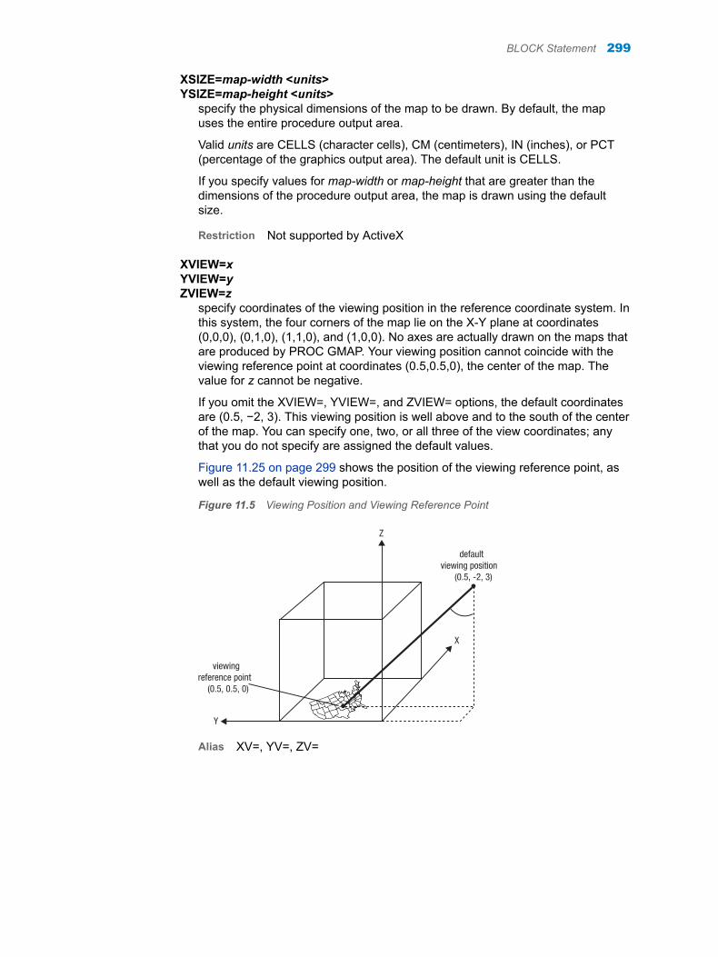
XSIZE=map-width <units>YSIZE=map-height <units>
specify the physical dimensions of the map to be drawn. By default, the map uses the entire procedure output area.
Valid units are CELLS (character cells), CM (centimeters), IN (inches), or PCT (percentage of the graphics output area). The default unit is CELLS.
If you specify values for map-width or map-height that are greater than the dimensions of the procedure output area, the map is drawn using the default size.
Restriction Not supported by ActiveX
XVIEW=xYVIEW=yZVIEW=z
specify coordinates of the viewing position in the reference coordinate system. In this system, the four corners of the map lie on the X-Y plane at coordinates (0,0,0), (0,1,0), (1,1,0), and (1,0,0). No axes are actually drawn on the maps that are produced by PROC GMAP. Your viewing position cannot coincide with the viewing reference point at coordinates (0.5,0.5,0), the center of the map. The value for z cannot be negative.
If you omit the XVIEW=, YVIEW=, and ZVIEW= options, the default coordinates are (0.5, −2, 3). This viewing position is well above and to the south of the center of the map. You can specify one, two, or all three of the view coordinates; any that you do not specify are assigned the default values.
Figure 11.25 on page 299 shows the position of the viewing reference point, as well as the default viewing position.
Figure 11.5 Viewing Position and Viewing Reference Point
viewingreference point
(0.5, 0.5, 0)
defaultviewing position
(0.5, -2, 3)
Z
X
Y
Alias XV=, YV=, ZV=
BLOCK Statement 299

Details
DescriptionThe BLOCK statement specifies the variable or variables that contain the data that are represented on the map by blocks of varying height, pattern, and color. This statement automatically performs the following operations:
n determines the midpoints ranges.
n scales the blocks.
n assigns patterns to the block faces and map areas. (See “About Block Maps and Patterns” on page 300 for more information.)
You can use statement options to enhance the appearance of the map. For example, you can specify the width and shape of the blocks, the outline colors for the blocks and the map areas, and the angle of view. Other statement options control the response levels.
In addition, you can use global statements to modify the block patterns, the map patterns, and the legend, as well as to add titles and footnotes to the map. You can also use an Annotate data set to enhance the map.
About Block Maps and PatternsBlock maps are different from other maps in that they display two different types of areas that use patterns:
n the blocks themselves, which represent the response levels
n the map areas from which the blocks rise
By default, block patterns are determined by the current style. When specifying the AREA statement or the AREA= option, the map area colors are determined by the current style and the block colors are determined by the specified attributes.
Note: If you specified the NOGSTYLE system option, then solid patterns are used for blocks and hatch patterns are used for the map areas. The map areas and their outlines use the first color in the color list.
The BLOCK statement has the following options that explicitly control the outline colors used by the blocks and the map areas:
n CBLKOUT=
n CEMPTY=
n COUTLINE=
In addition, the AREA= option and AREA statement control how the map areas are patterned.
When you use PATTERN statements to define the patterns for the map, you must specify the correct type of pattern for the area. The blocks use bar and block patterns and the map areas use map and plot patterns. See “PATTERN Statement” on page 78 for more information about specifying patterns.
300 Chapter 11 / GMAP Procedure

Note: If you specify only one PATTERN statement and include only the COLOR= option, that color is used for both the blocks and the map areas. For example, this statement makes the blocks solid blue and the map areas blue hatch.
pattern1 color=blue;
Note: If you specify a PATTERN statement to define a non-solid fill pattern but do not specify the BLOCK statement’s SHAPE=OLD option, the blocks are filled with solid patterns.
CHORO StatementCreates two-dimensional maps in which values of the specified response variables are represented by varying patterns and colors.
Requirement: At least one response variable is required. The ID statement must be used in conjunction with the CHORO statement
Supported Statements:
FOOTNOTE , NOTE, LEGEND, PATTERN, TITLE
SyntaxCHORO response-variable(s) </ options>;
Summary of Optional ArgumentsAppearance options
ANNOTATE=Annotate-data-setspecifies a data set to annotate onto maps that are produced by the CHORO statement.
CDEFAULT=empty-area-fill-colorfills empty map areas in the specified color.
CEMPTY=empty-area-outline-coloroutlines empty map areas in the specified color.
COUTLINE=area-outline-color | SAMEoutlines non-empty map areas in the specified color.
OSM<=(<STYLE=osmstyle> <AUTOPROJECT>)>specifies an OpenStreetMap (OSM) style and can project the unprojected map areas from latitude and longitude degrees onto the OSM map.
STRETCHstretches map extents to cover all available space in the device.
UNIFORM
CHORO Statement 301

causes the same legend and coloring to be used for all maps produced by the procedure instead of being calculated within each BY group for each map.
WOUTLINE=area-outline-widthspecifies the width of all map area outlines, in pixels.
XSIZE=map-width <units>YSIZE=map-height <units>
specify the physical dimensions of the map.
Description optionsDESCRIPTION="description"
specifies a description of the output.NAME="name"
specifies the name of the GRSEG catalog entry and the name of the graphics output file, if one is created.
Legend optionsCTEXT=text-color
specifies a color for the text in the legend.LEGEND=LEGEND<1 …99>
assigns the specified LEGEND statement that is to be applied to the map.NOLEGEND
suppresses the legend.
Mapping optionsDISCRETE
generates a separate response level (color and surface pattern) for each different value of the formatted response variable.
LEVELS=number-of-response-levels | ALLspecifies the number of response levels to be graphed for the response variable.
MIDPOINTS=value-list | OLDspecifies the response levels for the range of response values that are represented by each level (pattern and color combination).
MISSINGaccepts a missing value as a valid level for the response variable.
PERCENTcauses GMAP to collect all response values (or their statistic) and chart each region as a percentage of the whole.
RANGEdisplays value ranges in the legend.
STATFMT=format-specificationoverrides the GMAP default format for percent of PERCENT8.2.
STATISTIC=FIRST | SUM | FREQUENCY | MEANspecifies the statistic for GMAP to chart.
ODS optionsHTML_LEGEND=variable
identifies the variable in the input data set whose values create links or data tips or both.
HTML=variable
302 Chapter 11 / GMAP Procedure

identifies the variable in the input data set whose values create links or data tips or both.
URL=character-variablespecifies a character variable whose values are URLs.
Required Argumentresponse-variable(s)
specifies one or more variables in the response data set. Each response variable produces a separate map. All variables must be in the input data set. Multiple response variables are separated with blanks.
Missing values for the response variable are not considered valid response values unless you use the MISSING option in the CHORO statement.
Response variables can be either numeric or character in type. Numeric response variables are normally grouped into ranges, or response levels, as determined by default, or by the MIDPOINTS= or LEVELS=number-of-response-levels options. Each response level is assigned a different combination of pattern and color. With the LEVELS=ALL option, numeric or character response variables are assigned unique response levels, as are numeric variables when the DISCRETE option is specified. The LEVELS=number-of-response-levels option is ignored when either the DISCRETE or MIDPOINTS= option is used.
See “About Response Variables” on page 273.
Optional ArgumentsOptions in a CHORO statement affect all graphs that are produced by that statement. You can specify as many options as you want and list them in any order.
ANNOTATE=Annotate-data-setspecifies a data set to annotate onto maps that are produced by the CHORO statement.
Alias ANNO=
See “Overview: The Annotate Facility” in SAS/GRAPH: Reference
Example “Example 12: Using GfK GeoMarketing Map Data When Labeling Provinces on a Map” on page 384
CDEFAULT=empty-area-fill-colorfills empty map areas in the specified color. This option affects only map areas that are empty. Empty map areas are generated in choro maps only when there is no response value for a map area and the MISSING option is not used. They are also generated when a map area is omitted from the response data set and the ALL option is included in the PROC GMAP statement.
The default is NONE, which draws the polygon empty, showing the background in the fill area of the polygon.
Alias CDEF=, DEFCLR=
See The CEMPTY option, the “ALL” on page 279, and “Displaying Map Areas and Response Data” on page 274
CHORO Statement 303

CEMPTY=empty-area-outline-coloroutlines empty map areas in the specified color. This option affects only the empty map areas, which are generated in choro maps when either of the following is true:
n There is no response value for a map area and the MISSING option is not used.
n A map area is omitted from the response data set and the ALL option is included in the PROC GMAP statement.
The default outline color is the same as the default COUTLINE= color.
Alias CE=
See The option “ALL” on page 279 and “Displaying Map Areas and Response Data” on page 274.
COUTLINE=area-outline-color | SAMEoutlines non-empty map areas in the specified color. When COUTLINE=area-outline-color and DEVICE=ACTIVEX, both empty and non-empty map areas are outlined. The value SAME specifies that the outline color of a map area is the same as the interior pattern color.
The default outline color is determined by the current style. If you specified the NOGSTYLE system option, then the default color is black for ActiveX and the first color in the color list for all other devices.
Alias CO=
Note If you specify empty map patterns (VALUE=EMPTY in a PATTERN statement), then you should not change the outline color from the default value SAME to a single color. Otherwise, all the outlines are one color and you cannot distinguish between the empty areas.
CTEXT=text-colorspecifies a color for the text in the legend. If you omit the CTEXT= option, a color specification is searched for in this order:
n the CTEXT= option in a GOPTIONS statement.
n the default, the text color that is specified in the current style.
n If you specified the NOGSTYLE system option, then the default color is black for ActiveX and the first color in the color list for all other devices.
The CTEXT= color specification is overridden if you also use the COLOR= suboption of a LABEL= or VALUE= option in a LEGEND definition that is assigned to the map legend. The COLOR= suboption determines the color of the legend label or the color of the legend value descriptions, respectively.
Alias CT=
DESCRIPTION="description"specifies a description of the output. The maximum length for description is 256 characters. The description does not appear in the output. The descriptive text is shown in each of the following:
n the chart description for web output (depending on the device driver). See “Chart Descriptions for Web Presentations” in SAS/GRAPH: Reference for more information.
304 Chapter 11 / GMAP Procedure

n the Table of Contents that is generated when you use the CONTENTS= option in an ODS HTML statement, assuming that the output is generated while the contents page is open.
n the description and the properties for the output in the Results window.
n the description and properties for the catalog entry in the Explorer.
n the Description field of the PROC GREPLAY window.
The description can include the #BYLINE, #BYVAL, and #BYVAR substitution options, which work as they do when used on TITLE, FOOTNOTE, and NOTE statements. Refer to “Substituting BY Line Values in a Text String” on page 112. The 256-character limit applies before the substitution takes place for these options. Thus, if in the SAS program the entry-description text exceeds 256 characters, it is truncated to 256 characters, and then the substitution is performed.
Alias DES=
Default CHOROPLETH MAP OF variable-name
DISCRETEgenerates a separate response level (color and surface pattern) for each different value of the formatted response variable.
The LEVELS=number-of-response-levels option is ignored when you use the DISCRETE option.
If you specify the DISCRETE option, then distinct, non-continuous colors are used for the response values. If you specify the LEVELS= option, then a color ramp is used to assign each response value a continuous color scheme.
Note If the data does not contain a value in a particular range of the format, that formatted range is not displayed in the legend.
HTML=variableidentifies the variable in the input data set whose values create links or data tips or both. The variable values are either links or data tips or both that are created in the HTML file generated by the ODS statement. The links are URLs pointing to web pages to display when the user clicks (drills down) on elements in the graph. Data tips are detailed information or data values that are displayed as pop-up text when a mouse pointer is positioned over elements in the graph.
Interaction When multiple observations exist in the input data set for one variable value, the first observation is used for the data tip. When that same input data set is used for an annotate data set, the last of the multiple observations is used for the annotation. Sort the data one way for the data tip and the opposite way for the annotation to alleviate any mismatch between the data tip and its annotation in the resulting graph.
See “Data Tips for Web Presentations” in SAS/GRAPH: Reference
“Adding Links and Enhancements with the URL=, HTML=, and HTML_LEGEND= Options” in SAS/GRAPH: Reference
HTML_LEGEND=variableidentifies the variable in the input data set whose values create links or data tips or both. Input data set variable values are either links or data tips or both that are created in the HTML file generated by the ODS statement. The links are
CHORO Statement 305

associated with a legend value and point to the URL to display when the user clicks (drills down) on the value. Data tips are detailed information or data values that are displayed as pop-up text when a mouse pointer is positioned over values in the legend.
Restriction Not supported by ActiveX
See “Adding Links and Enhancements with the URL=, HTML=, and HTML_LEGEND= Options” in SAS/GRAPH: Reference
LEGEND=LEGEND<1 …99>assigns the specified LEGEND statement that is to be applied to the map. The LEGEND= option is ignored if the specified LEGEND definition is not currently in effect. In the GMAP procedure, the CHORO statement produces a legend by default unless you specify the NOLEGEND option. If you use the SHAPE= option in a LEGEND statement, then only the value BAR is valid. Most of the LEGEND options described in “LEGEND Statement” on page 56 are supported by ActiveX. If a LEGEND option is not supported by ActiveX, it is noted in the LEGEND option definition.
Restriction Partially supported by ActiveX
See “LEGEND Statement” on page 56
Example “Example 5: Using GfK GeoMarketing Map Data to Assign a Format to the Response Variable” on page 363
LEVELS=number-of-response-levels | ALLspecifies the number of response levels to be graphed for the response variable.
If you specify LEVELS=ALL, then all unique numeric or character response variable values are graphed.
Each response level is assigned a different surface pattern and color combination.
If you specify the LEVELS= option, then a color ramp is used to assign each response value a continuous color scheme. The response values are assigned lighter and darker values of a color scheme to express lower and higher response values. If you specify the DISCRETE option, then distinct, non-continuous colors are used for the response values.
If neither the LEVELS= option nor the DISCRETE option is used, then the GMAP procedure determines the number of response levels by using the formula FLOOR(1+3.3 log(n)), where n is the number of response variable values.
By default, an equal-distribution (quantizing) algorithm is used to determine each level.
When MIDPOINTS=OLD is used with the LEVELS= option, default midpoints are generated using the Nelder algorithm (Applied Statistics 25:94–7, 1976).
Restriction The LEVELS=number-of-response-levels option is ignored when you use the DISCRETE or MIDPOINTS=value-list option. It is also ignored when the response variables are character.
Note If you specified the NOGSTYLE system option, then noncontinuous colors are used by default.
Example “Example 3: Using GfK GeoMarketing Map Data to Specify Response Levels in a Block Map” on page 358
306 Chapter 11 / GMAP Procedure

MIDPOINTS=value-list | OLDspecifies the response levels for the range of response values that are represented by each level (pattern and color combination).
For numeric response variables, the value-list argument is either an explicit list of values, a starting value and an ending value with an interval increment, or a combination of both forms:
n n < ...n>
n n TO n <BY increment >
n n < ...n> TO n <BY increment > n < ...n>
By default the increment value is 1. You can specify discrete numeric values in any order. In all forms, n can be separated by blanks or commas. For example: midpoints=(2 4 6) midpoints=(2,4,6) midpoints=(2 to 10 by 2)
If a numeric variable has an associated format, the specified values must be the unformatted values.
For character response variables, value-list is a list of unique character values enclosed in quotation marks and separated by blanks:
n 'value-1' < ...'value-n'>
The values are character strings enclosed in single quotation marks and separated by blanks. For example: midpoints="Midwest" "Northeast" "Northwest"
Specify the values in any order. If a character variable has an associated format, the specified values must be the formatted values.
You can selectively exclude some response variable values from the map, as shown here: midpoints="Midwest"
The only observations that are shown on the map are those observations for which the response variable exactly matches one of the values that are listed in the MIDPOINTS= option. As a result, observations might be excluded inadvertently if values in the list are misspelled or if the case does not match exactly.
Specifying MIDPOINTS=OLD generates default midpoints using the Nelder algorithm (Applied Statistics 25:94–7, 1976).
See The RANGE option
Example “Example 17: Using GfK GeoMarketing Map Data When Specifying Midpoints in a Prism Map” on page 396
MISSINGaccepts a missing value as a valid level for the response variable.
See “Displaying Map Areas and Response Data” on page 274
NAME="name"specifies the name of the GRSEG catalog entry and the name of the graphics output file, if one is created.
The following applies to name:
n The name can be up to 256 characters in length.
n Special characters in the name are converted to underscores.
CHORO Statement 307

n For the GRSEG entry name:
o The name is truncated to eight characters.
o The first character is always represented in uppercase, and all other characters are represented in lowercase.
o If the name begins with a number, an underscore is prepended to the name.
o If the name duplicates an existing name, SAS/GRAPH appends a number or increments the last number used to create a unique graph name (for example, name1, name2, and so on). If necessary, the name is truncated so that the name and appended number do not exceed eight characters.
n For the graphics output filename:
o The filename is based on the NAME= value except when you use an ODS LISTING destination, a DEVICE= option, and a file reference specifying an output filename. In this case, the file reference specification overrides the NAME= value. See “Controlling Graphics Output for ODS LISTING” in SAS/GRAPH: Reference.
o All characters are represented in lowercase.
o If a number is added to the GRSEG name, the same number is added to the output filename. See “About Filename Indexing” in SAS/GRAPH: Reference.
o If the NAME= value is 8 characters or less, the filename is the GRSEG entry name.
o If the NAME= value is greater than 8 characters, the NAME= value is used as the filename. When an index number is used in the GRSEG entry name, that index number is appended to the output filename. See “About Filename Indexing” in SAS/GRAPH: Reference.
Note: If the name begins with a number, an underscore is prepended to the filename.
o The maximum allowable filename length is device-specific. If the length of the name exceeds the maximum for the graphics device, an error results and no graphics output file is generated.
Default GMAP
NOLEGENDsuppresses the legend.
Example “Example 12: Using GfK GeoMarketing Map Data When Labeling Provinces on a Map” on page 384
OSM<=(<STYLE=osmstyle> <AUTOPROJECT>)>specifies an OpenStreetMap (OSM) style and can project the unprojected map areas from latitude and longitude degrees onto the OSM map. This is an appearance option that enables you to use the OpenStreetMap (OSM) map as a background map. You can specify no suboptions, or use either a STYLE= suboption or an AUTOPROJECT suboption, or both suboptions.
If you specify the OSM option without any suboptions, the GMAP procedure by default uses the SASMAPNIK style and does not project the map.
If you specify the STYLE=osmstyle suboption only, the GMAP procedure uses one of the supported OSM styles that are appropriate for the map that you are
308 Chapter 11 / GMAP Procedure
processing (for example, SASMAPNIK or SASMAPNIK_LITE). Because the AUTOPROJECT suboption is not specified, the GMAP procedure does not project the map.
If you specify the OSM option with the AUTOPROJECT suboption only, the GMAP procedure projects the map area from latitude and longitude coordinates (in degrees) onto the OSM map. Because the STYLE suboption is not specified, the procedure uses the default SASMAPNIK style.
If you specify the OSM option with both the STYLE= and AUTOPROJECT suboptions, then the GMAP procedure uses one of the supported OSM styles that are appropriate for the map that you are processing. It projects the map area from latitude and longitude coordinates (in degrees) onto the OSM map.
Alias SHOWOSM
Default The default STYLE is SASMAPNIK. The map is not projected unless you specify the AUTOPROJECT suboption.
Restrictions The OSM option supports only the JAVAIMG device.
If the map area is already projected, do not specify the AUTOPROJECT suboption, or you will receive unexpected results.
PERCENTcauses GMAP to collect all response values (or their statistic) and chart each region as a percentage of the whole. You can use the STATISTIC= option to change how the percentage is calculated—whether as a percentage of the SUM, FREQUENCY, or MEAN. If you do not use the STATISTIC= option, then STATISTIC=FIRST is assumed–the response variable of only the first observation of each region is counted. If the response variable is a text field, then STATISTIC=FREQUENCY is used, even if you specify a different value for the STATISTIC= option.
Alias PERCENTAGE
See The “STATFMT=format-specification” on page 309 and the “STATISTIC=FIRST | SUM | FREQUENCY | MEAN” on page 310.
RANGEcauses GMAP to display, in the legend, the starting value and ending value of the range around each midpoint specified with the MIDPOINTS= option (instead of displaying just the midpoints). For example, if MIDPOINTS=15 25 35, then the legend could show 10-20, 20-30, 30-40.
Restrictions The MIDPOINTS= option must be specified for the RANGE option to have any effect.
Not supported by ActiveX
STATFMT=format-specificationoverrides the GMAP default format for percent of PERCENT8.2. Use this format when using calculated values. The STATFMT option is typically used when the STATISTIC=FREQUENCY option or the PERCENT option is used.
Alias SFMT=, SFORMAT=, STATFORMAT=
CHORO Statement 309

STATISTIC=FIRST | SUM | FREQUENCY | MEANspecifies the statistic for GMAP to chart. For character variables, FREQUENCY is the only allowed value—any other value is changed to FREQUENCY and a warning is issued. The frequency of a variable does not include missing values unless the MISSING option is specified.
FIRSTGMAP matches the first observation from the DATA= data set and charts the response value from this observation only. This is the default. If more rows exist that are not processed, a warning is issued to the log.
SUMAll observations matching a given ID value are added together and the summed value is charted.
FREQUENCYA count of all rows with nonmissing values is charted unless you specify the MISSING option.
MEANAll observations matching a given ID value are added together and then divided by the number of nonmissing observations matched. This value is then charted unless you specify the MISSING option.
Alias STAT=
STRETCHstretches map extents to cover all available space in the device. This might cause the map to be distorted. When this option is applied to the PROC GMAP statement, it applies to all statements. If applied to a single statement, it applies only to that statement.
Alias STRETCHTOFIT, STR2FIT
Restriction Not supported by ActiveX
UNIFORMcauses the same legend and coloring to be used for all maps produced by the procedure instead of being calculated within each BY group for each map. The UNIFORM option prescans the data to generate a categorization across all the data, regardless of BY grouping, and applies that categorization to all maps in the BY group. This results in all maps uniformly displaying legends and coloring such that a single value always has the same color in multiple maps.
When specified in a PROC GMAP statement, UNIFORM applies to all AREA, BLOCK, CHORO, and PRISM statements included within the GMAP run-group.
When omitted from the PROC GMAP statement, and specified on an individual AREA, BLOCK, CHORO, or PRISM statement, UNIFORM applies only to the maps produced by that statement.
URL=character-variablespecifies a character variable whose values are URLs. The variable values are URLs for web pages to display when the user clicks (drills down) on elements in the graph. The variable values are URLs for web pages to display when the user clicks (drills down) on elements in the graph.
Restriction This option affects graphics output that is created through the ODS HTML destination only.
310 Chapter 11 / GMAP Procedure

Interaction If you specify both the HTML= and URL= options, then the URL= option is ignored
See “Overview of Enhancing Web Presentations” in SAS/GRAPH: Reference
“Example: GIF Output with Drill-Down Links” in SAS/GRAPH: Reference
WOUTLINE=area-outline-widthspecifies the width of all map area outlines, in pixels.
Default 1
XSIZE=map-width <units>YSIZE=map-height <units>
specify the physical dimensions of the map. By default, the map uses the entire procedure output area.
Valid units are CELLS (character cells), CM (centimeters), IN (inches), or PCT (percentage of the graphics output area). The default unit is CELLS.
If you specify values for units that are greater than the dimensions of the procedure output area, the map is drawn using the default size.
You can specify only one of the XSIZE= or YSIZE= options. In this case the GMAP procedure scales the dimension for the unspecified option in order to retain the original shape of the map.
Restriction Not supported by ActiveX
Details
DescriptionThe CHORO statement specifies the variable or variables that contain the data represented on the map by patterns that fill the map areas. This statement automatically
n determines the midpoints
n assigns patterns to the map areas
You can use statement options to enhance the appearance of the map (for example, by selecting the colors and patterns that fill the map areas). Other statement options control the selection of ranges for the response variable.
In addition, you can use global statements to modify the map area patterns and legend, as well as add titles and footnotes to the map. You can also use an Annotate data set to enhance the map.
CHORO Statement 311

PRISM StatementCreates three-dimensional prism maps in which levels of magnitude of the specified response variables are represented by polyhedrons (raised polygons) of varying height, pattern, and color.
Requirement: At least one response variable is required. You must use the ID statement in conjunction with the PRISM statement.
Supported Statements:
FOOTNOTE , NOTE, LEGEND, PATTERN, TITLE
Note: For best results, use the MAPSSAS library of map data sets.
SyntaxPRISM response-variable(s) </ options>;
Summary of Optional ArgumentsAppearance options
ANNOTATE=Annotate-data-setspecifies a data set to annotate onto the maps that are produced by the PRISM statement.
CDEFAULT=empty-area-fill-colorfills empty map areas in the specified color.
CDEFAULT=empty-area-fill-colorfills empty map areas in the specified color.
CEMPTY=empty-area-outline-coloroutlines empty map areas in the specified color.
COUTLINE=area-outline-color | SAMEoutlines nonempty map areas in the specified color.
STRETCHstretches map extents to cover all available space in the device.
UNIFORMcauses the same legend and coloring to be used for all maps produced by the procedure instead of being calculated within each BY group for each map.
WOUTLINE=area-outline-widthspecifies the width, in pixels, of all map area outlines.
XLIGHT=xYLIGHT=y
specify the coordinates of the imaginary light source in the map coordinate system.
XSIZE=map-width <units>YSIZE=map-height <units>
312 Chapter 11 / GMAP Procedure

specify the dimensions of the map that you are drawing.XVIEW=x YVIEW=yZVIEW=z
specify the viewing position coordinates for the map.
Description optionsDESCRIPTION="description"
specifies a description of the output.NAME="name"
specifies the name of the GRSEG catalog entry and the name of the graphics output file, if one is created.
Legend optionsCTEXT=text-colorLEGEND=LEGEND<1 …99>
specifies the LEGEND definition to associate with the map.NOLEGEND
suppresses the legend.
Mapping optionsAREA=n | column-name
specifies that a different map pattern be used for the surface of each map area or group of map areas on the map.
DISCRETEgenerates a separate response level (color and surface pattern) for each different value of the formatted response variable.
LEVELS=number-of-response-levels | ALLspecifies the number of response levels to be graphed for the response variable.
MIDPOINTS=value-list | OLDspecifies the response levels for the range of response values that are represented by each level (prism height, pattern, and color combination).
MISSINGaccepts a missing value as a valid level for the response variable.
PERCENTcauses GMAP to collect all response values (or their statistic) and chart each region as a percentage of the whole.
RANGERELZERO
creates area heights that are relative to a zero value.STATFMT=format-specification
overrides the GMAP default format for percent of PERCENT8.2.STATISTIC=FIRST | SUM | FREQUENCY | MEAN
specifies the statistic for GMAP to chart.
ODS optionsHTML_LEGEND=variable
identifies the variable in the input data set whose values create links or data tips or both.
HTML=variable
PRISM Statement 313

identifies the variable in the input data set whose values create links or data tips or both.
URL=character-variablespecifies a character variable whose values are URLs.
Required Argumentresponse-variable(s)
specifies one or more variables in the response data set. Each response variable produces a separate map. All variables must be in the input data set. Multiple response variables are separated with blanks.
Missing values for the response variable are not considered valid unless you use the MISSING option.
Response variables can be either numeric or character. By default, and as determined by the LEVELS= or MIDPOINTS= values, numeric response variables are grouped into ranges, or response levels. Each response level is assigned a different prism height and a different pattern and color combination. With the LEVELS=ALL option, numeric or character response variables are assigned unique response levels, as are numeric variables when the DISCRETE option is specified. The LEVELS=number-of-response-levels option is ignored when either the DISCRETE or MIDPOINTS= option is used.
See “About Response Variables” on page 273.
Optional ArgumentsOptions in a PRISM statement affect all of the graphs that are produced by that statement. You can specify as many options as you want and list them in any order.
ANNOTATE=Annotate-data-setspecifies a data set to annotate onto the maps that are produced by the PRISM statement. Annotate coordinate systems 1, 2, 7, and 8 are not valid with Prism maps.
Alias ANNO=
See “Overview: The Annotate Facility” in SAS/GRAPH: Reference
AREA=n | column-namespecifies that a different map pattern be used for the surface of each map area or group of map areas on the map.
You can specify pattern fills or colors or both with PATTERN statements that specify map and plot patterns. A separate PATTERN definition is needed for each specified area.
AREA=nThe value of n indicates which variable in the ID statement determines the groups that are distinguished by a surface pattern. By default, all map unit areas are drawn using the same surface fill pattern. If your ID statement has only one map area identification variable, then use AREA=1 to indicate that each map area surface uses a different pattern. If you have more than one variable in your ID statement, then use n to indicate the position of the variable that defines groups that share a pattern. When you use the AREA=
314 Chapter 11 / GMAP Procedure
option, the map data set should be sorted in order of the variables in the ID statement.
AREA=column-nameA column name defined in either the MAP= or DATA= data sets can be indicated with the column-name value. If the column name exists in both the MAP= and DATA= data sets, the column in the map= data set is used. When column-name is used, the areas are colored based on the AREA= value. Duplicate AREA= values might be assigned different patterns.
Note The AREA statement provides a greater amount of control than the AREA= option.
See “AREA Statement” on page 283, “PATTERN Statement” on page 78.
CDEFAULT=empty-area-fill-colorfills empty map areas in the specified color. This option affects only map areas that are empty. Empty map areas are generated in prism maps only when there is no response value for a map area and the MISSING option is not used. They are also generated when a map area is omitted from the response data set and the ALL option is included in the PROC GMAP statement.
The default is NONE, which draws the polygon empty, showing the background in the fill area of the polygon.
Alias CDEF=, DEFCLR=
See The CEMPTY option, the “ALL” on page 279, and “Displaying Map Areas and Response Data” on page 274
CEMPTY=empty-area-outline-coloroutlines empty map areas in the specified color. Empty map areas are generated in prism maps either
n when there is no response value for a map area and the MISSING option is not used, or
n when a map area is omitted from the response data set and the ALL option is included in the PROC GMAP statement.
The default outline color is the same as the default COUTLINE= color.
Alias CE=
See “ALL” on page 279 and “Displaying Map Areas and Response Data” on page 274
CDEFAULT=empty-area-fill-colorfills empty map areas in the specified color. This option affects only map areas that are empty. Empty map areas are generated in prism maps only when there is no response value for a map area and the MISSING option is not used. They are also generated when a map area is omitted from the response data set and the ALL option is included in the PROC GMAP statement.
The default is NONE, which draws the polygon empty, showing the background in the fill area of the polygon.
Alias CDEF=, DEFCLR=
See The CEMPTY option, the “ALL” on page 279, and “Displaying Map Areas and Response Data” on page 274
PRISM Statement 315

COUTLINE=area-outline-color | SAMEoutlines nonempty map areas in the specified color. SAME specifies that the outline color of a map area is the same as the interior pattern color.
The default outline color is determined by the current style. If you specified the NOGSTYLE system option, then the default color is the first color in the color list.
Alias CO=
Note If you specify empty map patterns (VALUE=EMPTY in a PATTERN statement), you should not change the outline color from the default value SAME to a single color. Otherwise, all the outlines are one color and you cannot distinguish between the empty areas.
CTEXT=text-colorspecifies a color for the text in the legend. If you omit the CTEXT= option, a color specification is searched for in this order:
n the CTEXT= option in a GOPTIONS statement.
n the default, the text color that is specified in the current style.
n If you specified the NOGSTYLE system option, then the default color is black for ActiveX and the first color in the color list for all other devices.
The CTEXT= color specification is overridden if you also use the COLOR= suboption of a LABEL= or VALUE= option in a LEGEND definition assigned to the map legend. The COLOR= suboption determines the color of the legend label or the color of the legend value descriptions, respectively.
Alias CT=
DESCRIPTION="description"specifies a description of the output. The maximum length for description is 256 characters. The description does not appear in the output. The descriptive text is shown in each of the following:
n the chart description for web output (depending on the device driver). See “Chart Descriptions for Web Presentations” in SAS/GRAPH: Reference for more information.
n the Table of Contents that is generated when you use the CONTENTS= option in an ODS HTML statement, assuming that the output is generated while the contents page is open.
n the description and the properties for the output in the Results window.
n the description and properties for the catalog entry in the Explorer.
n the Description field of the PROC GREPLAY window.
The description can include the #BYLINE, #BYVAL, and #BYVAR substitution options, which work as they do when used on TITLE, FOOTNOTE, and NOTE statements. Refer to “Substituting BY Line Values in a Text String” on page 112. The 256-character limit applies before the substitution takes place for these options. Thus, if in the SAS program the entry-description text exceeds 256 characters, it is truncated to 256 characters, and then the substitution is performed.
Alias DES=
Default PRISM MAP OF variable-name
316 Chapter 11 / GMAP Procedure

DISCRETEgenerates a separate response level (color and surface pattern) for each different value of the formatted response variable.
The LEVELS=number-of-response-levels option is ignored when you use the DISCRETE option.
If you specify the DISCRETE option, then distinct, non-continuous colors are used for the response values. If you specify the LEVELS= option, then a color ramp is used to assign each response value a continuous color scheme.
Note If the data does not contain a value in a particular range of the format, that formatted range is not displayed in the legend.
HTML=variableidentifies the variable in the input data set whose values create links or data tips or both. The variable values are either links or data tips or both that are created in the HTML file generated by the ODS statement. The links are URLs pointing to web pages to display when the user clicks (drills down) on elements in the graph. Data tips are detailed information or data values that are displayed as pop-up text when a mouse pointer is positioned over elements in the graph.
Interaction When multiple observations exist in the input data set for one variable value, the first observation is used for the data tip. When that same input data set is used for an annotate data set, the last of the multiple observations is used for the annotation. Sort the data one way for the data tip and the opposite way for the annotation to alleviate any mismatch between the data tip and its annotation in the resulting graph.
See “Data Tips for Web Presentations” in SAS/GRAPH: Reference
“Adding Links and Enhancements with the URL=, HTML=, and HTML_LEGEND= Options” in SAS/GRAPH: Reference
HTML_LEGEND=variableidentifies the variable in the input data set whose values create links or data tips or both. Input data set variable values are either links or data tips or both that are created in the HTML file generated by the ODS statement. The links are associated with a legend value and point to the URL to display when the user clicks (drills down) on the value. Data tips are detailed information or data values that are displayed as pop-up text when a mouse pointer is positioned over values in the legend..
Restriction Not supported by ActiveX
See “Adding Links and Enhancements with the URL=, HTML=, and HTML_LEGEND= Options” in SAS/GRAPH: Reference
LEGEND=LEGEND<1 …99>specifies the LEGEND definition to associate with the map. LEGEND= is ignored if the specified LEGEND definition is not currently in effect. In the GMAP procedure, the PRISM statement produces a legend unless you use the NOLEGEND option. If you use the SHAPE= option in a LEGEND statement, only the value BAR is valid. Most of the LEGEND options described in “LEGEND Statement” on page 56 are supported by ActiveX. If a LEGEND option is not supported by ActiveX, it is noted in the LEGEND option definition.
PRISM Statement 317

Restriction Partially supported by ActiveX
See “LEGEND Statement” on page 56
Example “Example 17: Using GfK GeoMarketing Map Data When Specifying Midpoints in a Prism Map” on page 396
LEVELS=number-of-response-levels | ALLspecifies the number of response levels to be graphed for the response variable.
If you specify LEVELS=ALL, then all unique numeric or character response variable values are graphed.
Each response level is assigned a different surface pattern and color combination. The prism height is based on the data value of the corresponding response variable.
If you specify the LEVELS= option, then a color ramp is used to assign each response value a continuous color scheme. The response values are assigned lighter and darker values of a color scheme to express lower and higher response values. If you specify the DISCRETE option, then distinct, non-continuous colors are used for the response values.
If neither the LEVELS= option nor the DISCRETE option is used, then the GMAP procedure determines the number of response levels by using the formula FLOOR(1+3.3 log(n)), where n is the number of response variable values.
By default, an equal-distribution (quantizing) algorithm is used to determine each level.
When MIDPOINTS=OLD is used with the LEVELS= option, default midpoints are generated using the Nelder algorithm (Applied Statistics 25:94–7, 1976).
Restriction The LEVELS=number-of-response-levels option is ignored when you use the DISCRETE or MIDPOINTS=value-list option. It is also ignored when the response variables are character.
Example “Example 3: Using GfK GeoMarketing Map Data to Specify Response Levels in a Block Map” on page 358
MIDPOINTS=value-list | OLDspecifies the response levels for the range of response values that are represented by each level (prism height, pattern, and color combination).
For numeric response variables, value-list is either an explicit list of values, or a starting value and an ending value with an interval increment, or a combination of both forms:
n n < ...n>
n n TO n <BY increment>
n n < ...n> TO n <BY increment > n < ...n>
By default the increment value is 1. You can specify discrete numeric values in any order. In all forms, n can be separated by blanks or commas. An example is: midpoints=(2 4 6) midpoints=(2,4,6) midpoints=(2 to 10 by 2)
If a numeric variable has an associated format, the specified values must be the unformatted values.
For character response variables, value-list has this form:
318 Chapter 11 / GMAP Procedure

n 'value-1' < ...'value-n'>
The values are character strings enclosed in single quotation marks and separated by blanks, as shown here: midpoints="Midwest" "Northeast" "Northwest"
Specify the values in any order. If a character variable has an associated format, the specified values must be the formatted values.
You can selectively exclude some response variable values from the map, as shown here: midpoints="Midwest"
Only those observations for which the response variable exactly matches one of the values listed in the MIDPOINTS= option are shown on the map. As a result, observations might be inadvertently excluded if values in the list are misspelled or if the case does not match exactly.
Specifying MIDPOINTS=OLD generates default midpoints using the Nelder algorithm (Applied Statistics 25:94–7, 1976).
See The RANGE option
Example “Example 17: Using GfK GeoMarketing Map Data When Specifying Midpoints in a Prism Map” on page 396
MISSINGaccepts a missing value as a valid level for the response variable.
See “Displaying Map Areas and Response Data” on page 274
NAME="name"specifies the name of the GRSEG catalog entry and the name of the graphics output file, if one is created.
The following applies to name:
n The name can be up to 256 characters in length.
n Special characters in the name are converted to underscores.
n For the GRSEG entry name:
o The name is truncated to eight characters.
o The first character is always represented in uppercase, and all other characters are represented in lowercase.
o If the name begins with a number, an underscore is prepended to the name.
o If the name duplicates an existing name, SAS/GRAPH appends a number or increments the last number used to create a unique graph name (for example, name1, name2, and so on). If necessary, the name is truncated so that the name and appended number do not exceed eight characters.
n For the graphics output filename:
o The filename is based on the NAME= value except when you use an ODS LISTING destination, a DEVICE= option, and a file reference specifying an output filename. In this case, the file reference specification overrides the NAME= value. See “Controlling Graphics Output for ODS LISTING” in SAS/GRAPH: Reference.
o All characters are represented in lowercase.
PRISM Statement 319

o If a number is added to the GRSEG name, the same number is added to the output filename. See “About Filename Indexing” in SAS/GRAPH: Reference.
o If the NAME= value is 8 characters or less, the filename is the GRSEG entry name.
o If the NAME= value is greater than 8 characters, the NAME= value is used as the filename. When an index number is used in the GRSEG entry name, that index number is appended to the output filename. See “About Filename Indexing” in SAS/GRAPH: Reference.
Note: If the name begins with a number, an underscore is prepended to the filename.
o The maximum allowable filename length is device-specific. If the length of the name exceeds the maximum for the graphics device, an error results and no graphics output file is generated.
Default GMAP
NOLEGENDsuppresses the legend.
PERCENTcauses GMAP to collect all response values (or their statistic) and chart each region as a percentage of the whole. You can use the STATISTIC= option to change how the percentage is calculated—whether as a percentage of the SUM, FREQUENCY, or MEAN. If you do not use the STATISTIC= option, then STATISTIC=FIRST is assumed and the response variable of only the first observation of each region is counted. If the response variable is a text field, then STATISTIC=FREQUENCY is used, even if you specify a different value for the STATISTIC= option.
Alias PERCENTAGE
See The “STATFMT=format-specification” on page 321, and the “STATISTIC=FIRST | SUM | FREQUENCY | MEAN” on page 321.
RANGEcauses GMAP to display, in the legend, the starting value and ending value of the range around each midpoint specified with the MIDPOINTS= option (instead of displaying just the midpoints). For example, if MIDPOINTS=15 25 35, then the legend could show 10-20, 20-30, 30-40.
Restriction MIDPOINTS= must be specified for the RANGE option to have any effect. Not supported by ActiveX.
RELZEROcreates area heights that are relative to a zero value. By default, GMAP creates heights that are relative to the minimum value, which might or might not be zero. With the RELZERO option, zero value areas have no height.
Alias REL0, RELATIVETOZERO
Restriction This option works only for variables that have no negative values.
320 Chapter 11 / GMAP Procedure

STATFMT=format-specificationoverrides the GMAP default format for percent of PERCENT8.2. Use this format when using calculated values. The STATFMT option is typically used when the STATISTIC=FREQUENCY option or the PERCENT option is used.
Alias SFMT=, SFORMAT=, STATFORMAT=
STATISTIC=FIRST | SUM | FREQUENCY | MEANspecifies the statistic for GMAP to chart. For character variables, FREQUENCY is the only allowed value—any other value is changed to FREQUENCY and a warning is issued. The frequency of a variable does not include missing values unless the MISSING option is specified.
FIRSTGMAP matches the first observation from the DATA= data set and charts the response value from this observation only. This is the default. If more rows exist that are not processed, a warning is issued to the log.
SUMAll observations matching a given ID value are added together and the summed value is charted.
FREQUENCYA count of all rows with nonmissing values is charted unless you specify the MISSING option.
MEANAll observations matching a given ID value are added together and then divided by the number of nonmissing observations matched. This value is then charted unless you specify the MISSING option.
Alias STAT=
STRETCHstretches map extents to cover all available space in the device. This might cause the map to be distorted. When this option is applied to the PROC GMAP statement, it applies to all statements. If applied to a single statement, it applies only to that statement.
Alias STRETCHTOFIT, STR2FIT
Restriction Not supported by ActiveX
UNIFORMcauses the same legend and coloring to be used for all maps produced by the procedure instead of being calculated within each BY group for each map. The UNIFORM option prescans the data to generate a categorization across all the data, regardless of BY grouping, and applies that categorization to all maps in the BY group. This results in all maps uniformly displaying legends and coloring such that a single value always has the same color in multiple maps.
When specified in a PROC GMAP statement, the UNIFORM option applies to all AREA, BLOCK, CHORO, and PRISM statements included within the GMAP run-group.
When omitted from the PROC GMAP statement, and specified on an individual AREA, BLOCK, CHORO, or PRISM statement, the UNIFORM option applies only to the maps produced by that statement.
PRISM Statement 321

URL=character-variablespecifies a character variable whose values are URLs. The variable values are URLs for web pages to display when the user clicks (drills down) on elements in the graph.
Restriction This option affects graphics output that is created through the ODS HTML destination only.
Interaction If you specify both the HTML= option and the URL= option, then the URL= option is ignored.
See “Overview of Enhancing Web Presentations” in SAS/GRAPH: Reference
“Example: GIF Output with Drill-Down Links” in SAS/GRAPH: Reference
WOUTLINE=area-outline-widthspecifies the width, in pixels, of all map area outlines.
Default 1
XLIGHT=xYLIGHT=y
specify the coordinates of the imaginary light source in the map coordinate system. The position of the light source affects how the sides of the map polygons are shaded. Although you can specify any point for the light source using the XLIGHT= and YLIGHT= options, the light source is actually placed in one of only four positions.
Table 11.26 on page 322 shows how the point that you specify is positioned. It correlates a specified light source in the left column with the coordinate position of that light source in the right column.
Table 11.5 Light Source Coordinates
Specified light source Light source position
In quadrants I or II, or on the X or +Y axis
Behind the map (point A), and all side polygons are shadowed
On or within approximately 10 degrees of the Y axis
The viewing position (point D), and none of the side polygons are shadowed
In quadrant III (except within 10 degrees of the Y axis)
To the left of the map (point B), and the right-facing sides of polygons are shadowed
In quadrant IV (except within 10 degrees of the Y axis)
To the right of the map (point C), and the left-facing side polygons are shadowed
322 Chapter 11 / GMAP Procedure

Figure 11.26 on page 323 illustrates the light source positions. Assume that your viewing position, selected by the XVIEW=, YVIEW=, and ZVIEW= options, is point D.
Figure 11.6 Coordinates of Imagined Light Source in a Map Coordinate System
A
D
B C
III
III IV
X
Y
By default, the light source position is the same as the viewing position specified by the XVIEW=, YVIEW=, and ZVIEW= options. The light source position cannot coincide with the viewing reference point (0.5,0.5), which corresponds with the position directly above the center of the map.
Restriction Not supported by ActiveX
See “XVIEW=x |YVIEW=y| ZVIEW=z” on page 323
XSIZE=map-width <units>YSIZE=map-height <units>
specify the dimensions of the map that you are drawing. By default, the map uses the entire procedure output area.
Valid units are CELLS (character cells), CM (centimeters), IN (inches), or PCT (percentage of the graphics output area). The default unit is CELLS.
If you specify values for map-width and map height that are greater than the dimensions of the procedure output area, the map is drawn using the default size. If you specify one value and not the other, the dimension is adjusted to maintain the correct aspect ratio.
Restriction Not supported by ActiveX
XVIEW=xYVIEW=yZVIEW=z
specify the viewing position coordinates for the map. In this system, the four corners of the map lie on the X–Y plane at coordinates (0, 0, 0), (0, 1, 0), (1, 1, 0), and (1, 0, 0).
PRISM Statement 323

The viewing position cannot coincide with the viewing reference point at coordinates (0.5, 0.5, 0).
The value for z cannot be negative.
If you omit the XVIEW=, YVIEW=, and ZVIEW= options, the default coordinates are (0.5, −2,3). This viewing position is well above and to the south of the center of the map. One, two, or all three view coordinates can be specified; any that are not specified are assigned the default values.
Figure 11.25 on page 299 shows the position of the viewing reference point, as well as the default viewing position.
To ensure that the polygon edges are distinguishable, the angle from vertical must be less than or equal to 45 degrees. If you specify such a small ZVIEW= value that this condition cannot be satisfied, then PROC GMAP increases the ZVIEW= value automatically so that the angle is 45 degrees or less.
Alias XV=, YV=, ZV=
Details
DescriptionThe PRISM statement specifies the variable or variables that contain the data that are represented on the map by raised map areas. This statement automatically performs the following operations:
n determines the midpoints ranges or midpoints
n assigns patterns to the map areas
You can use statement options to control the ranges of the response values, specify the angle of view, and enhance the appearance of the map.
In addition, you can use global statements to modify the map area patterns and the legend, as well as add titles and footnotes to the map. You can also use an Annotate data set to enhance the map.
Note: PRISM maps do not work well with polygons within polygons (holes). It is recommended that a CHORO or BLOCK map be created for these maps instead.
SURFACE StatementCreates three-dimensional surface maps in which levels of magnitude of the specified response variables are represented by spikes of varying height.
Restriction: Not supported by ActiveX
Requirement: At least one response variable is required and must be numeric. The ID statement must be used in conjunction with the SURFACE statement.
324 Chapter 11 / GMAP Procedure
Supported Statement:
TITLE, FOOTNOTE, NOTE
SyntaxSURFACE response-variable(s) </ options>;
Summary of Optional ArgumentsAppearance options
ANNOTATE=Annotate-data-setspecifies a data set to annotate onto maps that are produced by the SURFACE statement.
CBODY=surface-map-colorspecifies the color that is used to draw the surface map.
CONSTANT=nspecifies a denominator to use in the distance decay function.
NLINES=number-of-linesspecifies the number of lines used to draw the surface map.
ROTATE=degreesspecifies the degrees of the angle at which to rotate the map about the Z axis in the map coordinate system.
TILT=degreesspecifies the degrees of the angle at which to tilt the map about the X axis in the map coordinate system.
XSIZE=map-width <units>YSIZE=map-height <units>
specify the physical dimensions of the map.
Description optionsDESCRIPTION="description"
specifies a description of the output.NAME="name"
specifies the name of the GRSEG catalog entry and the name of the graphics output file, if one is created.
Mapping optionsPERCENT
causes GMAP to collect all response values (or their statistic) and chart each region as a percentage of the whole.
STATFMT=format-specificationoverrides the GMAP default format for percent of PERCENT8.2.
STATISTIC=FIRST | SUM | FREQUENCY | MEANspecifies the statistic for GMAP to chart.
SURFACE Statement 325

Required Argumentresponse-variable(s)
specifies one or more variables in the response data set. The response-variable must be numeric and must contain only positive values. Each response variable produces a separate map. All variables must be in the input data set. Multiple response variables are separated with blanks.
The GMAP procedure scales response variables for presentation on the map. The height of the spikes on the map correspond to the relative value of the response variable, not to the actual value of the response variable. However, when the viewing angle is changed, the spikes might not appear this way. The spikes in the front might appear to be higher than the spikes in the back, which represent greater values.
See “About Response Variables” on page 273.
Optional ArgumentsSURFACE statement options affect all maps that are produced by that statement.
ANNOTATE=Annotate-data-setspecifies a data set to annotate onto maps that are produced by the SURFACE statement. Annotate coordinate systems 1, 2, 7, and 8 are not valid with surface maps.
Alias ANNO=
See “Overview: The Annotate Facility” in SAS/GRAPH: Reference
CBODY=surface-map-colorspecifies the color that is used to draw the surface map. Regardless of the current ODS style, the default color is the first color in the current color list.
Alias CB=
CONSTANT=nspecifies a denominator to use in the distance decay function. This function determines the base width of the spike that is drawn at each map area center.
By default, CONSTANT=10. Values greater than 10 yield spikes that are wider at the base. Values less than 10 yield spikes that are narrower at the base.
Alias CON=
DESCRIPTION="description"specifies a description of the output. The maximum length for description is 256 characters. The description does not appear in the output. The descriptive text is shown in each of the following:
n the chart description for web output (depending on the device driver). See “Chart Descriptions for Web Presentations” in SAS/GRAPH: Reference for more information.
n the Table of Contents that is generated when you use the CONTENTS= option in an ODS HTML statement, assuming that the output is generated while the contents page is open.
n the description and the properties for the output in the Results window.
326 Chapter 11 / GMAP Procedure

n the description and properties for the catalog entry in the Explorer.
n the Description field of the PROC GREPLAY window.
The description can include the #BYLINE, #BYVAL, and #BYVAR substitution options, which work as they do when used on TITLE, FOOTNOTE, and NOTE statements. Refer to “Substituting BY Line Values in a Text String” on page 112. The 256-character limit applies before the substitution takes place for these options. Thus, if in the SAS program the entry-description text exceeds 256 characters, it is truncated to 256 characters, and then the substitution is performed.
Alias DES=
Default SURFACE MAP OF variable-name
NAME="name"specifies the name of the GRSEG catalog entry and the name of the graphics output file, if one is created.
The following applies to name:
n The name can be up to 256 characters in length.
n Special characters in the name are converted to underscores.
n For the GRSEG entry name:
o The name is truncated to eight characters.
o The first character is always represented in uppercase, and all other characters are represented in lowercase.
o If the name begins with a number, an underscore is prepended to the name.
o If the name duplicates an existing name, SAS/GRAPH appends a number or increments the last number used to create a unique graph name (for example, name1, name2, and so on). If necessary, the name is truncated so that the name and appended number do not exceed eight characters.
n For the graphics output filename:
o The filename is based on the NAME= value except when you use an ODS LISTING destination, a DEVICE= option, and a file reference specifying an output filename. In this case, the file reference specification overrides the NAME= value. See “Controlling Graphics Output for ODS LISTING” in SAS/GRAPH: Reference.
o All characters are represented in lowercase.
o If a number is added to the GRSEG name, the same number is added to the output filename. See “About Filename Indexing” in SAS/GRAPH: Reference.
o If the NAME= value is 8 characters or less, the filename is the GRSEG entry name.
o If the NAME= value is greater than 8 characters, the NAME= value is used as the filename. When an index number is used in the GRSEG entry name, that index number is appended to the output filename. See “About Filename Indexing” in SAS/GRAPH: Reference.
Note: If the name begins with a number, an underscore is prepended to the filename.
SURFACE Statement 327

o The maximum allowable filename length is device-specific. If the length of the name exceeds the maximum for the graphics device, an error results and no graphics output file is generated.
Default GMAP
NLINES=number-of-linesspecifies the number of lines used to draw the surface map. Values can range from 50 to 100; the higher the value, the more solid the map appears and the more resources used. By default, NLINES=50.
Alias N=
PERCENTcauses GMAP to collect all response values (or their statistic) and chart each region as a percentage of the whole. You can use the STATISTIC= option to change how the percentage is calculated—whether as a percentage of the SUM, FREQUENCY, or MEAN. If you do not use the STATISTIC= option, then STATISTIC=FIRST is assumed and the response variable of only the first observation of each region is counted. If the response variable is a text field, then STATISTIC=FREQUENCY is used, even if you specify a different value for the STATISTIC= option.
Alias PERCENTAGE
See The “STATFMT=format-specification” on page 328, and the “STATISTIC=FIRST | SUM | FREQUENCY | MEAN” on page 328.
ROTATE=degreesspecifies the degrees of the angle at which to rotate the map about the Z axis in the map coordinate system. The degrees argument can be any angle. Positive values indicate rotation in the counterclockwise direction. By default, ROTATE=70. The ROTATE= option also affects the direction of the lines that are used to draw the surface map.
STATFMT=format-specificationoverrides the GMAP default format for percent of PERCENT8.2. Use this format when using calculated values. The STATFMT option is typically used when the STATISTIC=FREQUENCY option or the PERCENT option is used.
Alias SFMT=, SFORMAT=, STATFORMAT=
STATISTIC=FIRST | SUM | FREQUENCY | MEANspecifies the statistic for GMAP to chart. For character variables, FREQUENCY is the only allowed value—any other value is changed to FREQUENCY and a warning is issued. The frequency of a variable does not include missing values unless the MISSING option is specified.
FIRSTGMAP matches the first observation from the DATA= data set and charts the response value from this observation only. This is the default. If more rows exist that are not processed, a warning is issued to the log.
SUMAll observations matching a given ID value are added together and the summed value is charted.
FREQUENCYA count of all rows with nonmissing values is charted unless you specify the MISSING option.
328 Chapter 11 / GMAP Procedure

MEANAll observations matching a given ID value are added together and then divided by the number of nonmissing observations matched. This value is then charted unless you specify the MISSING option.
Alias STAT=
TILT=degreesspecifies the degrees of the angle at which to tilt the map about the X axis in the map coordinate system. The value of degrees can be 0 to 90. Increasing values cause the map to tilt backward and makes the spikes more prominent. Decreasing values make the map shape more distinguishable and the spikes less prominent. TILT=90 corresponds to viewing the map edge-on, whereas TILT=0 corresponds to viewing the map from directly overhead. By default, TILT=70.
XSIZE=map-width <units>YSIZE=map-height <units>
specify the physical dimensions of the map. By default, the map uses the entire procedure output area.
Valid units are CELLS (character cells), CM (centimeters), IN (inches), or PCT (percentage of the graphics output area). The default unit is CELLS.
If you specify values for map-width and map-height that are greater than the dimensions of the procedure output area, the map is drawn using the default size. And if you specify only one dimension, the other is scaled to maintain the aspect ratio.
Details
DescriptionThe SURFACE statement specifies the variable or variables that contain the data that are represented on the map by raised map areas. This statement automatically determines the midpoints. You can use statement options to control spike proportions, specify the angle of view, and modify the general appearance of the map. For example, you can select the color and number of lines for the representation of the surface area. You can control the selection of spike heights and base widths.
In addition, you can use global statements to add titles and footnotes to the map. You can also enhance the map with an Annotate data set.
SURFACE Statement 329

Usage: GMAP Procedure
Using FIPS Codes and Province CodesThe map area identification variable in some SAS/GRAPH map data sets contain standardized numeric codes. The data sets for the United States contain a variable whose values are Federal Information Processing Standards (FIPS) codes. Traditional data sets for Canada contain standard province codes or census division codes. GfK data sets for Canada contain standard province codes and province names. You can specify a map data set with the GMAP procedure. However, ensure that the map area identification variable values in the map data set are the same as those used in the response data.
If the map area identification variables in your response data set are state or province names or abbreviations, convert them to FIPS codes or province codes before using the response data set with one of the traditional map data sets supplied by SAS. Conversion might not be necessary if one of the GfK map data sets is used. This is because character variables such as ID that contain region values, might already match the identification variables in your response data set. Table 11.27 on page 330 lists in two columns the FIPS codes for the United States and Table 11.28 on page 331 lists in two columns the standard codes for Canadian provinces.
Note: Alternatively, you can convert the FIPS code or province codes in your traditional map data set to match the names in your response data.
Table 11.6 U.S. FIPS Codes
FIPS code State
FIPS code State
01 Alabama 30 Montana
02 Alaska 31 Nebraska
04 Arizona 32 Nevada
05 Arkansas 33 New Hampshire
06 California 34 New Jersey
08 Colorado 35 New Mexico
330 Chapter 11 / GMAP Procedure

FIPS code State
FIPS code State
09 Connecticut 36 New York
10 Delaware 37 North Carolina
11 District of Columbia 38 North Dakota
12 Florida 39 Ohio
13 Georgia 40 Oklahoma
15 Hawaii 41 Oregon
16 Idaho 42 Pennsylvania
17 Illinois 44 Rhode Island
18 Indiana 45 South Carolina
19 Iowa 46 South Dakota
20 Kansas 47 Tennessee
21 Kentucky 48 Texas
22 Louisiana 49 Utah
23 Maine 50 Vermont
24 Maryland 51 Virginia
25 Massachusetts 53 Washington
26 Michigan 54 West Virginia
27 Minnesota 55 Wisconsin
28 Mississippi 56 Wyoming
29 Missouri 72 Puerto Rico
Table 11.7 Canadian Province Codes
Province code Province
10 Newfoundland and Labrador
Usage: GMAP Procedure 331

Province code Province
11 Prince Edward Island
12 Nova Scotia
13 New Brunswick
24 Quebec
35 Ontario
46 Manitoba
47 Saskatchewan
48 Alberta
59 British Columbia
60 Yukon
61 Northwest Territories
62 Nunavut
Note: The id-variables are numeric in traditional but character in GfK Canadian map data sets.
The MAPS.CNTYNAME data set contains a cross-reference of names and FIPS codes for all counties in the United States. The MAPS.CANCENS data set contains a cross-reference of census district names and codes for Canadian provinces.
Base SAS software provides several functions that convert state names to FIPS codes and vice versa. The following table lists these functions and a brief description of each. See SAS Functions and CALL Routines: Reference for more information.
Table 11.8 FIPS and SAS Postal Code Functions
Function Description
STFIPS Converts state postal code to FIPS state code
STNAME Converts state postal code to state name in uppercase
STNAMEL Converts state postal code to state name in mixed case
FIPNAME Converts FIPS code to state name in uppercase
332 Chapter 11 / GMAP Procedure

FIPNAMEL Converts FIPS code to state name in mixed case
FIPSTATE Converts FIPS code to state postal code
Using Formats for Traditional Map Data Set Variables
You can specify an output map area name or numeric value using one of the predefined formats for maps. The following prefixes are used in the names of the formats for maps:
CONTContinent
CNTRYCountry
GLCGeographic Location Code, distributed by Government Services Administration, USA
ISOInternational Standard Organization
The formats for maps are located in the SASHELP.MAPFMTS catalog. See the MAPS.NAMES table to view all the continent and country names and corresponding GLC, ISO, and numeric representation for the continent values.
To use one of the formats for maps, you must specify the SASHELP.MAPFMTS catalog on the FMTSEARCH= option in a SAS OPTIONS statement:
options fmtsearch=(sashelp.mapfmts);
In addition to using the PUT statement (as shown in the examples in the following table), the formats can also be invoked using a FORMAT statement. Each table row, from left to right, lists a SAS FORMAT statement, a description of what it does, a code example using the format, and the resulting output.
Note: If the input to a format is invalid, the format is “**” or “***” .
Table 11.9 Formats for Maps
FORMAT DESCRIPTION EXAMPLE OUTPUT
contfmt Use a continent's numeric value to output the continent's name
cont= 91put(cont,contfmt.);
North America
glcna Use the country's GLC numeric code to output the
id=460put(id,glcna.);
IR
Usage: GMAP Procedure 333

FORMAT DESCRIPTION EXAMPLE OUTPUT
country's GLC alpha code
glcnlu Use the GLC numeric code to output the country's long name in uppercase
id=460put(id,glcnlu.);
IRAN, ISLAMIC REPUBLIC OF
glcnsu Use the GLC numeric code to output the country's short name in uppercase
id=460put(id,glcnsu.);
IRAN
glcnsm Use the GLC numeric code to output the country's name in mixed case
id=460put(id,glcnsm.);
Iran
ison2a Use the country's ISO numeric code to output the country's ISO alpha2 code
iso=364put(iso,ison2a.);
IR
ison3a Use the country's ISO numeric code to output the country's ISO alpha3 code
iso=364put(iso,ison3a.);
IRN
isonlu Use the country's ISO numeric code to output the country's long name in uppercase
iso=364put(iso,isonlu.);
IRAN, ISLAMIC REPUBLIC OF
isonsu Use the country's ISO numeric code to output the country's short name in uppercase
iso=364put(iso,isonsu.);
IRAN
$cntrysl Use a country's short name in uppercase to output the country's long name in uppercase
name='IRAN'put(name,$cntrysl.);
IRAN, ISLAMIC REPUBLIC OF
$glcalu Use the GLC alpha code to output the country's long name in uppercase
country='IR'put(country,$glcalu.);
IRAN, ISLAMIC REPUBLIC OF
334 Chapter 11 / GMAP Procedure

FORMAT DESCRIPTION EXAMPLE OUTPUT
$glcan Use the country's GLC alpha code to output the country's GLC numeric code
country='IR'put(country,$glcan.);
460
$glcsua Use the country's short name in uppercase to output the GLC alpha code name
name='IRAN'put(name,$glcsua.);
IR
$glcsun Use the country's short name in uppercase to output the country's GLC numeric code
name='IRAN'put(name,$glcsun.);
460
$glcsma Use the country's short name in mixed-case to output the country's GLC alpha code
mixname='Iran'put(mixname,$glcsma.);
IR
$glcsmn Use the country's short name in mixed-case to output the country's GLC numeric code
mixname='Iran'put(mixname,$glcsmn.);
460
$glcprov Use a province or city name appended by || as a delimiter, followed by the country's GLC alpha code. This displays a province||country code, the province or city code, and the country's GLC alpha numeric code
provname='TEHRAN||IR'put(provname,$glcprov.);
8250460
8250 — province or city code
460 — country GLC numeric code
$isosu2a Use the country's short name in uppercase to display the country's ISO alpha2 code
name='IRAN'put(name,$isosu2a.);
IR
$isosu3a Use the country's name in uppercase to display the country's ISO alpha3 code
name='IRAN'put(name,$isosu3a.);
IRN
Usage: GMAP Procedure 335

FORMAT DESCRIPTION EXAMPLE OUTPUT
$isosun Use the country's short name in uppercase to display the country's ISO numeric code
name='IRAN'put(name,$isosun.);
364
$isoa2lu Use the country's ISO alpha2 code to display the country's long name in uppercase
alpha2='IR'put(alpha2,$isoa2su.);
IRAN, ISLAMIC REPUBLIC OF
$isoa2n Use the country's ISO alpha2 code to display the country's ISO numeric code
alpha2='IR'put(alpha2,$isoa2n.);
364
$isoa2su Use the country's ISO alpha2 code to display the country's short name in uppercase
alpha2='IR'put(alpha2,$isoa2lu.);
IRAN
$isoa3lu Use the country's ISO alpha3 code to display the country's long name in uppercase
alpha3='IRN'put(alpha3,$isoa3lu.);
IRAN, ISLAMIC REPUBLIC OF
$isoa3n Use the country's ISO alpha3 code to display the country's ISO numeric code
alpha3='IRN'put(alpha3,$isoa3n.);
364
$isoa3su Use the country's ISO alpha3 code to display the country's short name in uppercase
alpha3='IRN'put(alpha3,$isoa3su.);
IRAN
$isosm2a Use the country's short name in mixed-case to display the country's ISO alpha2 code
mixname='Iran'put(mixname,$isosm2a.);
IR
$isosm3a Use the country's short name in mixed-case to display the country's ISO alpha3 code
mixname='Iran'put(mixname,$isosm3a.);
IRN
336 Chapter 11 / GMAP Procedure

FORMAT DESCRIPTION EXAMPLE OUTPUT
$isosmn Use the country's short name in mixed-case to display the country's ISO numeric code
mixname='Iran'put(mixname,$isosmn.);
364
Using SAS/GRAPH Map Data Sets
Specifying the Location of Map Data SetsThere are three library references (librefs) associated with the location of a SAS library; each library containing map data sets used by SAS/GRAPH. The three are as follows:
n MAPS
n MAPSGFK
n MAPSSAS
You can download the latest map data sets from the SAS Maps and Geocoding website at https://support.sas.com/en/knowledge-base/maps-geocoding/maps-online.html. You are required to access the website with your SAS profile. You might be required to enter your site information.
MAPS references the library containing the latest set of SAS traditional maps. This library is defined in a configuration file with the value set to the same physical name (path) as MAPSSAS. For example, when specifying MAPS.UK, MAPS is the libref, and UK is a file in the SAS MAPS library.The libref is assigned through the “MAPS= System Option” on page 122. It can also be set or changed with a LIBNAME statement, which enables each client to set their own definition for MAPS. This client setting would override the server setting defined at start-up time. Note that using the “APPEND= System Option” in SAS System Options: Reference or the “INSERT= System Option” in SAS System Options: Referencewith the “MAPS= System Option” on page 122 allows an additional libref to be assigned to MAPS without changing its original definition. In this way existing programs can reference either the latest SAS or the MAPSGFK digital, vector map data sets.
MAPSGFK references the library containing the digital, vector map data sets at a location separate from the latest non-digital, vector SAS map data sets. This library is defined in a configuration file as a single physical path. This definition is set at installation time and should not be changed. The libref is assigned through the “MAPSGFK= System Option” on page 123.
MAPSSAS references the library containing the latest set of SAS traditional map files. This library is defined in a configuration file as a single physical name (path). It is the same path that MAPS references. This definition is set at installation time and
Usage: GMAP Procedure 337

should not be changed. The libref is assigned through the “MAPSSAS= System Option” on page 124.
Accessing Detailed Descriptions of Map Data SetsYou might need detailed information about the map data sets in order to determine their type, size, the variables that they contain, or, in the case of traditional map data sets, whether they are projected or unprojected. You can get this information by doing the following:
n using the CONTENTS or DATASETS procedure
n browsing the MAPS.METAMAPS data set in the MAPS library
n browsing the MAPSSAS.METAMAPS data set in the MAPSSAS library.
n browsing the library where your map data sets supplied by SAS reside
See “The METAMAPS Data Set” on page 269. Once the libref MAPS has been assigned, you can see a complete list of map data sets by viewing the MAPS.METAMAPS data set.
Run the following statements to list the map data sets in the SAS library that is assigned to the libref MAPS: Alternatively, you can substitute the libref MAPSGFK or MAPSSAS.
proc data sets lib=maps;run;
Run the following statements to provide detailed information about a map data set, including the number of observations, the variables in each data set, and a description of each variable:
proc contents data=maps.canada3;run;
To see the contents and descriptions of all of the map data sets associated with one of the three map libraries supplied by SAS, specify one of the following statements in the CONTENTS procedure:
n DATA=MAPS._ALL_
n DATA=MAPSSAS._ALL_
n DATA=MAPSGFK._ALL_
See the Base SAS Procedures Guide for more information about the CONTENTS and DATASETS procedures..
338 Chapter 11 / GMAP Procedure

Customizing SAS/GRAPH Map Data Sets
Overview of Customizing Map Data SetsYou can customize the area that is displayed on your map by using only part of a particular map data set. There are several ways to accomplish this. You can use WHERE processing or a DATA step to subset the map data to be used by the GMAP procedure.
You can also use the GPROJECT procedure with the map data set to create a rectangular subset of a map data set. Do this by using the minimum and maximum longitude and latitude values in the map data set. For more information, see Chapter 12, “GPROJECT Procedure,” on page 433.
You can combine map data sets in either of these situations:
n The map data sets to be combined were originally projected together.
n The map data sets all contain the same type of coordinates. That is, all are in radians or all are in degrees, and the longitude coordinates are measured in the same direction.
Map data sets supplied by SAS that contain coordinates expressed only as longitude and latitude, with variable names LONG and LAT, must be renamed X and Y. They should also be projected before you use them with the GMAP procedure. Map data sets from GfK GeoMarketing GmBH already contain projected coordinates expressed as longitude and latitude in degrees, with variable names LONG and LAT.
Subsetting Map Data SetsSome of the SAS/GRAPH map data sets contain a large number of observations. Programs that use only a few states or provinces run faster if you exclude the unused portion of the map data set or use a reduced map data set. SAS provides several ways to accomplish this. One is to use the WHERE statement or WHERE= data set option within the GMAP procedure to select only the states or provinces that you want.
The WHERE statement and WHERE= data set option are most useful when you produce a simple map and do not need to make any other changes to the data set. For example, to use only the observations for Quebec in the CANADA map data set, begin the GMAP procedure with this statement:
proc gmap map=maps.canada(where=(province="24"));
The WHERE= data set option applies only to the data set that you specify in the argument in which the WHERE= option appears. If you use the WHERE statement, the WHERE condition applies to the map data set and the response data set.
Another approach is to use a DATA step to create a subset of the larger data set. This code illustrates a way to extract the observations for Quebec from the CANADA map data set:
data quebec; set maps.canada(where=(province="24"));
Usage: GMAP Procedure 339

This approach is most useful when you want to create a permanent subset of a map data set. It is also useful when you need to make additional changes to the map data set.
See Chapter 14, “GREMOVE Procedure,” on page 485 for an example of how to use GREMOVE to create a regional map from one of the map data sets that are supplied with SAS/GRAPH.
Reducing Map Data SetsA reduced map data set is one that can be used to draw a map that retains the overall appearance of the original map but that contains fewer points. It requires considerably less storage space and can be drawn much more quickly. You can improve performance by plotting fewer observations for each map area. You reduce a map data set when you subset it on the variable DENSITY. You can add the variable DENSITY to a map data set by using the GREDUCE procedure. For more information, see Chapter 13, “GREDUCE Procedure,” on page 471.
Note: Many of the map data sets in the MAPS library are supplied with a DENSITY variable.
An unreduced map data set contains all of the coordinates that were produced when the map was digitized. This type of map data set has more observations than most graphics output devices can accurately plot. Some unreduced map data sets already contain a DENSITY variable like the one calculated by the GREDUCE procedure. Therefore, it is not necessary to use the GREDUCE procedure to process these data sets. Values for DENSITY range from 0 through 6 (the lower the density, the coarser the boundary line).
You can set the DENSITY value by using the DENSITY= option in the PROC GMAP statement. For example, the following statement excludes all points with a density level of 2 or greater:
proc gmap map=maps.states density=2;
The resulting map is much coarser than one drawn by using all of the observations in the data set, but it is drawn much faster.
Another way to create a reduced map data set is to use a DATA step to exclude observations with larger density values:
data states; set maps.states(where=(density<2));
Projecting Traditional Map Data SetsTraditional map data sets can be stored as unprojected or projected coordinates. GfK map data sets are stored as only projected. Unprojected map data sets contain spherical coordinates, that is, longitude and latitude values usually expressed in radians.1
Many of the map data sets in the MAPS library are projected. However, these map data sets contain only unprojected coordinates and should be projected before you use them.
1. If your data is in degrees, then it can be converted to radians by multiplying by the degree-to-radian constant [atan(1)/45].
340 Chapter 11 / GMAP Procedure

n CANADA3
n CANADA4
n COUNTIES
n COUNTY
n STATES
If the projection supplied with the map data set does not meet your needs, then you can use the GPROJECT procedure (on unprojected map coordinates) to create a different projection. For more information about map data sets with unprojected coordinates, see “Map Data Sets Containing X, Y, LONG, and LAT” on page 257. You should select a projection method that least distorts the regions that you are mapping. (All projection methods inherently distort map regions.) See Chapter 12, “GPROJECT Procedure,” on page 433 for more information.
Note: Using an unprojected map data set with the GMAP procedure can cause your map to be reversed.
Controlling the Display of Lakes and Landlocked AreasSome countries contain a lake or a polygonal area that is located completely within a single unit area. Occasionally these areas can be a problem when working with map data sets. In addition, displaying these areas might not be appropriate for some applications. In these cases, you might want to remove them from the map data set before you proceed.
In traditional and GfK map data sets that contain coordinates for a lake or area that is located within a single internal division, the area is identified with the numeric variable LAKE. The value of LAKE is 1 for points that correspond to water. A value of 2 indicates land points. A value of 0 corresponds to a landlocked area — an area within an internal region. Such an area would be visible as a hole in the resulting map graph. It is best to remove all such areas from the map data set by using LAKE=0. In the following programming code, the DATA step statements illustrate the inclusion of a lake in Denmark region DK-101. Then WHERE processing is used to delete the lake from that Denmark region. The first graph shows the Denmark region DK-101 with its lake, and second shows the same region without the lake.
data subset_map;set mapsgfk.denmark;if id in:('DK-101') then output;run;proc gmap map=subset_map data=subset_map res=none; id id; choro id / discrete stat=first; title "Lake in Denmark";run; where lake=0;title "Denmark with Lake Removed (Lake=0)";run;quit;
Usage: GMAP Procedure 341

Output 11.1 The DK-101 Region of Denmark with and Without Its Lake
342 Chapter 11 / GMAP Procedure

The following statements illustrate how to delete the lakes from your GfK map data sets using WHERE processing. The STAT=FIRST option processes only the first observation that matches the geographic region in the MAPSGFK map data set.
proc gmap map=mapsgfk.us_all(where=(lake=0)) data=mapsgfk.us_all; id id; choro id / levels=1 stat=first nolegend; title box=1 f=none h=4 "U.S. with Lakes Removed";run;quit;
Usage: GMAP Procedure 343

You can also create a new traditional map data set that is a subset of the traditional map data set:
data nolake; set maps.chile(where=(lake=0));run;
Creating SAS Map Data Sets
Creating Map Data Sets
OverviewIn addition to using map data sets that are supplied with SAS/GRAPH software, you can also create your own map data sets. Map data sets are not limited to geographic data; you use them to define other spaces such as floor plans.
When creating map data sets, the following variables must be included:
n a numeric variable named X that contains the horizontal coordinates of the boundary points. The value of this variable is projected and represents longitude when your data is geographic. When your data is not geographic but defines
344 Chapter 11 / GMAP Procedure

spaces such as floor plans, this variable might not be projected and might not represent longitude. This variable is required by the GMAP procedure.
n a numeric variable named Y that contains the vertical coordinates of the boundary points. The value of this variable is projected and represents latitude when your data is geographic. When your data is not geographic but defines spaces such as floor plans, this variable might not be projected and might not represent latitude. This variable is required by the GMAP procedure.
n one or more variables that uniquely identify the areas in the map. Map area identification variables can be either character or numeric and are indicated in the ID statement. An identification variable is required by the GMAP procedure.
The X and Y variable values in the map data set do not have to be in any specific units. They are rescaled by the GMAP procedure based on the minimum and maximum values in the data set. The minimum X and Y values are in the lower left corner of the map, and the maximum X and Y values are in the upper right corner.
The GMAP procedure uses the values of the X and Y variables to draw the map. To use the unprojected values to produce a custom map, follow the tasks in “Map Data Sets Containing X, Y, LONG, and LAT” on page 257.
Map data sets in which the X and Y variables contain unprojected longitude and latitude should be projected before you use them with PROC GMAP. See Chapter 12, “GPROJECT Procedure,” on page 433 for details.
Here are optional variables to consider including in map data sets:
n a numeric variable named DENSITY that holds the density values returned from a GREDUCE procedure.
n a numeric variable named LONG that contains the horizontal coordinate of the boundary point in degrees or radians. The value of this variable is unprojected and represents longitude (east-west position).
n a numeric variable named LAT that contains the vertical coordinate of the boundary point in degrees or radians. The value of this variable is unprojected and represents latitude (north-south position).
n a variable named SEGMENT to identify map areas that comprise noncontiguous polygons. Each unique value of the SEGMENT variable within a single map area defines a distinct polygon. If the SEGMENT variable is not present, each map area is drawn as a separate closed polygon that is regarded as a single segment.
The observations for each segment of a map area in the map data set must occur in the order in which the points are to be connected. The GMAP procedure forms map area outlines by connecting the boundary points of each segment in the order in which they appear in the data set. Eventually the last point is joined to the first point to complete the polygon. All the segments for each ID value must be contiguous within the map data set. The observations must be specified in a clockwise direction. However, an enclosed polygon (a hole representing a lake, for example) must be specified in a counter-clockwise direction—opposite from the direction in which the containing polygon is drawn.
n a variable named RESOLUTION to map detail level based on output resolution. Refer to Table 11.24 on page 267 for a list of the output resolutions associated with a RESOLUTION variable value.
A unit area is defined by observations in the map data set that have the same identification (ID) variable value. A unit area might be composed of a single polygon or a collection of polygons. A polygon is defined by all of the observations that have the same SEGMENT variable value within the same unit area.
Usage: GMAP Procedure 345

n If the unit area is a single polygon, then all values of SEGMENT are the same (alternatively, you can omit the SEGMENT variable).
n If the unit area contains multiple polygons, such as islands, then the SEGMENT variable has multiple values. For example, in the MAPS.US data set, the state of Hawaii (a unit area) contains six different values in the SEGMENT variable, one for each island in the state.
n If the unit area contains enclosed polygons (holes), such as lakes, then the SEGMENT variable has one value but the interior polygon is defined by separate boundaries. To separate boundaries, a missing X and Y value must be inserted at the separation point. For example, in the CANADA2 data set supplied with SAS/GRAPH, the map area for the Northwest Territories (a unit area) use enclosed polygons for two lakes.
Creating a Unit Area That Is a Single PolygonThis DATA step creates a SAS data set that contains coordinates for a unit area with a single polygon, a square:
data square; input id x y; datalines;1 0 01 0 401 40 401 40 0;
This data set does not have a SEGMENT variable.
Creating a Unit Area That Contains Multiple PolygonsUse different values of the SEGMENT variable to create separate polygons within a single unit area. For example, this DATA step assigns two values to the SEGMENT variable. The resulting data set produces a single unit area that contains two polygons, as shown in Figure 11.27 on page 347:
data map; input id $ segment x y; datalines;square 1 0 0square 1 0 4square 1 4 4square 1 4 0square 2 5 5square 2 5 7square 2 7 7square 2 7 5;
346 Chapter 11 / GMAP Procedure

Figure 11.7 Single Unit Area with Two Segments (Polygons)
Creating a Unit Area That Contains Enclosed Polygons as HolesUse separate boundaries to create an enclosed polygon (that is, a polygon that falls within the primary polygon for a single segment). The boundary for the hole is separated from the primary polygon boundary by inserting a missing value for X and Y. The last three observations are drawn counter-clockwise, in the opposite direction from the primary polygon. This enables an HTML image of the map to render correctly in all web browsers. For example, the data set that is created by this DATA step produces the map shown in Figure 11.28 on page 348:
data map; input id $ segment x y; datalines;square 1 0 0square 1 0 4square 1 4 4square 1 4 0square 1 . .square 1 3 1square 1 2 2square 1 1 1;
Usage: GMAP Procedure 347

Figure 11.8 Single Unit Area with Hole
Note: A single map segment is a section of a unit area with a single value of the SEGMENT variable. A single map segment cannot contain multiple polygons without having at least one observation with missing values for X and Y. All segments within the map data sets supplied by SAS/GRAPH contain a single polygon that can have one or more separate boundaries. Each boundary is separated by an observation with missing values for X and Y.
Creating a Unit Area That Contains Another AreaSometimes rather than a hole or lake, an enclosed polygon represents a separate map area. For example, in MAPS.AFRICA, the country of Lesotho is surrounded by the country of South Africa.
Note: As in some Traditional map data sets, MAPS.AFRICA specifies the coordinates to draw both country polygons in a clockwise direction. This might adversely affect the rendering of the HTML image of the map in some web browsers.
To create an enclosed map area:
1 Create an observation with missing values for X and Y for the surrounding area.
2 Define the boundary as part of the surrounding area by the using ID value for the surrounding area.
3 Define the boundary as part of the enclosed area by using the ID value for the enclosed area.
The triangle observations are drawn counter-clockwise, in the opposite direction from the hole in the primary (square) polygon. This enables an HTML image of the map to render correctly in all web browsers.
348 Chapter 11 / GMAP Procedure

For example, this DATA step creates a data set that produces the map shown in Figure 11.29 on page 349:
data map; input id $ segment x y; datalines;square 1 0 0square 1 0 4square 1 4 4square 1 4 0square 1 . .square 1 1 1square 1 2 2square 1 3 1triangle 1 3 1triangle 1 2 2triangle 1 1 1;
Figure 11.9 Unit Area within a Unit Area
Usage: GMAP Procedure 349

Using GfK Map Data Sets with Existing Code
Reworking Code That Uses Traditional Map Data Sets
OverviewThis section presents several examples of existing code that uses traditional map data sets, with tips for repurposing the code to use a GfK map data set and variables. The existing code fragment is shown first, followed by the code rewritten with the recommended changes. The tips and details of the change are presented as /* comments */ within each section of rewritten code.
Code to Prepare a Choropleth Map of AfghanistanIf you have existing code similar to the following:
proc gmap data=mydata map=maps.afghanis;id id;choro id / nolegend;run;
Rewrite the code as follows to use a GfK map data set and ensure that the id-variable, in this case ID, is a matching character format between the response data set and the input data set:
/* Change the traditional map data set name (maps.afghanis) *//* to the GfK map data set name (mapsgfk.afghanistan). *//* The id-variable value in mydata must match the */ /* GfK id-variable character format. *//* GfK id-variables ID and ID1 are character format. */proc gmap data=mydata map=mapsgfk.afghanistan;id id;choro id / nolegend;run;
Code to Prepare a Map of Europe for AnnotationIf you have existing code similar to the following:
proc gmap data=mydata map=maps.europe;id id;choro id / levels=1 nolegend anno=mypoints;run;
350 Chapter 11 / GMAP Procedure

Rewrite the code as follows to use a GfK map data set and a different id-variable because ID is now character format:
/* Change the traditional map data set name (maps.europe) *//* to the GfK map data set name (mapsgfk.europe). *//* If the id-variable value in 'mydata' is numeric choose the *//* GfK id-variable SEGMENT, which is also numeric format, or create *//* your own variable. *//* Note that GfK id-variables ID and ID1 are character format. *//* The LEVELS=<number-of-midpoints> option will only work with numeric */ /* response variable values. */proc gmap data=mydata map=mapsgfk.europe;id;choro segment / levels=1 nolegend anno=mypoints;run;
Code to Prepare a United States Map After Projecting Spherical Coordinates (Longitude and Latitude)If you have existing code similar to the following, which projects the X and Y coordinate units in radians:
proc gproject data=maps.states out=mystates project=lambert;id state;run;
proc gmap data=mydata map=mystates;id state;choro state / nolegend;run;
Rewrite the code as follows to use the GfK map data set and the projected X and Y coordinates (in degrees) provided in the input data set:
/* Change the traditional map data set name (maps.states) to the *//* GfK map data set name mapsgfk.us_states. *//* Remove Proc GPROJECT and use the provided projected coordinates in degrees. */proc gmap data=mydata map=mapsgfk.us_states;id state;choro state / nolegend;run;
Code to Project Annotate Data with a GfK Map Data SetUse the following code to project only the Annotate data and not the already projected map:
/* The mapsgfk.projparm data set contains input projection parameters. */
Usage: GMAP Procedure 351

/* Project the points using the map's projection parameters stored that data set. *//* The us_states entry in the projection parameters data set is used for *//* input parameters. */ /* mapsgfk.us_states is the GfK map data set for the United States that *//* contains unprojected longitude (X) and latitude (Y) variables in radians. */
proc gproject data=anno out=annoproj parmin=mapsgfk.projparm parmentry=us_states;run;
proc gmap data=mydata map=mapsgfk.us_states anno=annoproj;id state;choro state / nolegend;run;
Usage Tips with GfK Map Data Sets
Best PracticesWhen using the GfK map data set named US_ALL, the character identification variable ID uniquely refers to the state_county in the United States as well as other U.S. Territories. Specifying the variable ID instead of STATE ensures that the polygons are drawn correctly. For example:
proc gmap data=mydata map=mapsgfk.us_all;id id;choro id;run;
If you want to use the STATE variable, use it in combination with the COUNTY identification variable:
proc gmap data=mydata map=mapsgfk.us_all;id state county;choro id;run;
To more accurately create a map for the island nation of Maldives in the Indian Ocean, use the most current MAPSGFK.WORLD or the MAPSGFK.MALDIVES data sets. You might have existing code that uses the traditional MAPS.WORLD data set. In that case, you can achieve the same level of map detail by using this data set version from SAS 9.1M3.
It is a requirement that each GfK map data set completes any enclosed polygons (holes) it contains in a counter-clockwise direction. This is the opposite direction from which the hole in the containing polygon is drawn. This enables an HTML map
352 Chapter 11 / GMAP Procedure

image to render correctly in all web browsers. It also enables any HTML hover-text to display correctly for an area containing a hole without interfering with that hole.
Note: Traditional map data sets vary in the direction in which they complete enclosed polygons (holes). For example, the MAPS.AFRICA data set completes enclosed polygons in a clockwise direction. Traditional map data sets were created before the setting of map data set requirements to enable viewing HTML in web browsers.
Examples: GMAP Procedure
Example 1: Using GfK GeoMarketing Map Data to Produce a Simple Block MapFeatures: MAP= required argument referring to GfK map data
DATA= argument referring to response dataID statementRESOLUTION= optionBLOCK statement options
BLOCKSIZE=COUTLINE=RELZERO
System option FMTSEARCH=SQL procedurePATTERN statement
Data sets: MAPSGFK.ASIA (map data set)DEMOGRAPHICS (table of response data)
Format: ison2a
Restriction: The GfK GeoMarketing map data set used in this example is licensed to be used only with SAS/GRAPH.
Sample library member:
GMPGSIMP
Notes: The SAS Sample Library is not available in SAS Studio.You can download the mapping samples in the SAS Sample Library in zipped format from the SAS/GRAPH Learning and Support page on support.sas.com. Click the link for SAS/GRAPH and Base SAS: Mapping Reference (Examples ZIP).The map data set or data sets supplied by SAS and used in this program might not be an available resource on your system.The ISO codes that are in the sashelp.demographics data set are not as recent as the ISO codes found in the MAPSGFK data set.
Example 1: Using GfK GeoMarketing Map Data to Produce a Simple Block Map 353

OutputThis example uses a GfK map data set to produce a block map that shows the population of countries in Asia. Because the DISCRETE option is not used, the response variable is assumed to have a continuous range of values. Because neither the LEVELS= nor MIDPOINTS= option is used, the GMAP procedure selects a number of levels based on the number of map areas. It then calculates the appropriate response levels. The elongated countries in the displayed map indicate that a different projection method was used with this GfK map than was used with the traditional Asia map data set.
Programoptions fmtsearch=(sashelp.mapfmts);
proc sql; create table demographics(rename=(iso=oiso newiso=iso id=oldid newid=ID)) asselect demo.*, put(demo.iso,z3.) as newiso format=$3.,put(demo.iso,ison2a.) as newid from sashelp.demographics as demo
354 Chapter 11 / GMAP Procedure

;alter table demographicsmodify ID char(15) label='Alpha2 Country Code';quit;
goptions reset=all border;
title1 "Population in Asia";legend1 label=(position=top) shape=bar(.3in,.1in);footnote1 j=r "This map drawn with GfK map data";pattern1 value=msolid color=tan;
proc gmap data=demographics(where=(cont=95)) map=mapsgfk.asia resolution=4 all; id iso; block pop / blocksize=1 relzero coutline=gray legend=legend1;run;quit;
Program DescriptionSpecify the format catalog to search that has the predefined ISO alpha2 code.
options fmtsearch=(sashelp.mapfmts);
Create a table named demographics using sashelp.demographics as the base and change its variables to match GfK variable types and lengths. This table is used as the response data set. This step makes two changes to the sashelp.demographics data set. The ISO variable is converted from numeric to character. Secondly, a character ID variable is created. This ID value matches the character variable ISOALPHA2 value in the GfK map data set. The format 'ison2a' is used to convert the numeric ISO code to its equivalent ISOALPHA2 code.
proc sql; create table demographics(rename=(iso=oiso newiso=iso id=oldid newid=ID)) asselect demo.*, put(demo.iso,z3.) as newiso format=$3.,put(demo.iso,ison2a.) as newid from sashelp.demographics as demo;alter table demographicsmodify ID char(15) label='Alpha2 Country Code';quit;
Set the graphics environment.
goptions reset=all border;
Define the title, legend, footnote, and color for the map. The PATTERN statement specifies a solid tan color pattern for the Asian continent, differentiating it from the block colors.
title1 "Population in Asia";legend1 label=(position=top) shape=bar(.3in,.1in);footnote1 j=r "This map drawn with GfK map data";pattern1 value=msolid color=tan;
Example 1: Using GfK GeoMarketing Map Data to Produce a Simple Block Map 355

Produce the block map. Specify the demographics table just created as the response data set. Specify a GfK map data set named mapsgfk.asia. Specifically use the Asia continent. The RESOLUTION= option specifies that all map observations with a RESOLUTION variable value of 4 or less be used. The 4 value corresponds to a resolution of 800 x 600 pixels. ALL specifies that the generated map should include all the map areas from the map data set, even if there is no observation for that map area. The ID statement specifies the variable that is in both the map data set and the response data set and defines map areas. Note that the ISO variable is character. The BLOCK statement specifies the population variable in the response data set that contains the response values for each of the map areas. The BLOCKSIZE= option specifies the width of the blocks. The RELZERO option specifies that the block values are relative to zero. The COUTLINE= option specifies a gray color for the map outline so that the blocks are highly visible.
proc gmap data=demographics(where=(cont=95)) map=mapsgfk.asia resolution=4 all; id iso; block pop / blocksize=1 relzero coutline=gray legend=legend1;run;quit;
Example 2: Using Traditional Map Data to Produce a Simple Block MapFeatures: MAP= required argument referring to traditional map data set
DATA= required argument referring to response dataID statementBLOCK statement options
BLOCKSIZE=RELZERO
PATTERN statement
Data sets: MAPS.ASIA (map data set)SASHELP.DEMOGRAPHICS (response data)
Sample library member:
GMPSIMPL
Notes: The SAS Sample Library is not available in SAS Studio.You can download the mapping samples in the SAS Sample Library in zipped format from the SAS/GRAPH Learning and Support page on support.sas.com. Click the link for SAS/GRAPH and Base SAS: Mapping Reference (Examples ZIP).The map data set or data sets supplied by SAS and used in this program might not be an available resource on your system.
OutputThis example produces a block map that shows population of countries in Asia. Because the DISCRETE option is not used, the response variable is assumed to
356 Chapter 11 / GMAP Procedure

have a continuous range of values. Because neither the LEVELS= nor MIDPOINTS= option is used, the GMAP procedure selects a number of levels based on the number of map areas. It then calculates the appropriate response levels.
Programgoptions reset=all border;
title1 "Population in Asia";pattern1 value=msolid color=tan;
proc gmap data=sashelp.demographics(where=(cont=95)) map=maps.asia all; id id; block pop / blocksize=1 relzero;run;quit;
Program DescriptionSet the graphics environment.
goptions reset=all border;
Define the title and the color for the map. The PATTERN statement specifies a solid tan color pattern for the Asian continent, differentiating it from the block colors.
title1 "Population in Asia";
Example 2: Using Traditional Map Data to Produce a Simple Block Map 357

pattern1 value=msolid color=tan;
Produce the block map. The ALL argument specifies that the output should include all of the map areas from the map data set. This happens even if the response data set SASHELP.DEMOGRAPHICS does not include an observation for the map area. The ID statement specifies the variable that is in both the map data set and the response data set and defines map areas. The BLOCK statement specifies the variable in the response data set that contains the response values for each of the map areas. The BLOCKSIZE= option specifies the width of the blocks. The RELZERO option specifies that the block values are relative to zero.
proc gmap data=sashelp.demographics(where=(cont=95)) map=maps.asia all; id id; block pop / blocksize=1 relzero;run;quit;
Example 3: Using GfK GeoMarketing Map Data to Specify Response Levels in a Block MapFeatures: MAP= required argument referring to a GfK map data set
DATA= argument referring to response dataID statementBLOCK statement options
LEVELS=SHAPE=RELZEROCEMPTY=
System option FMTSEARCH=SQL procedurePATTERN statement
Data sets: MAPSGFK.SAMERICA (map data set)DEMOGRAPHICS (table of response data)
Format: ison2a
Restriction: The GfK GeoMarketing map data set used in this example is licensed to be used only with SAS/GRAPH.
Sample library member:
GMPGLEVL
Notes: The SAS Sample Library is not available in SAS Studio.You can download the mapping samples in the SAS Sample Library in zipped format from the SAS/GRAPH Learning and Support page on support.sas.com. Click the link for SAS/GRAPH and Base SAS: Mapping Reference (Examples ZIP).The map data set or data sets supplied by SAS and used in this program might not be an available resource on your system.The ISO codes that are in the sashelp.demographics data set are not as recent as the ISO codes found in the MAPSGFK data set.
358 Chapter 11 / GMAP Procedure

OutputThis example uses the LEVELS= option to specify the number of response levels for the blocks. The LEVELS= option tells GMAP how many response levels and the GMAP procedure calculates the quantiles.
Programoptions fmtsearch=(sashelp.mapfmts);
proc sql;create table demographics(rename=(iso=oiso newiso=iso id=oldid newid=ID)) asselect demo.*, put(demo.iso,z3.) as newiso format=$3.,put(demo.iso,ison2a.) as newid from sashelp.demographics as demo;alter table demographicsmodify ID char(15) label='Alpha2 Country Code';quit;
goptions reset=all border;
title1 "Gross National Income per Capita";title2 "South America";footnote1 j=r "This map drawn with GfK map data";pattern1 value=msolid color=tan;
proc gmap data=demographics(where=(cont=92))
Example 3: Using GfK GeoMarketing Map Data to Specify Response Levels in a Block Map 359
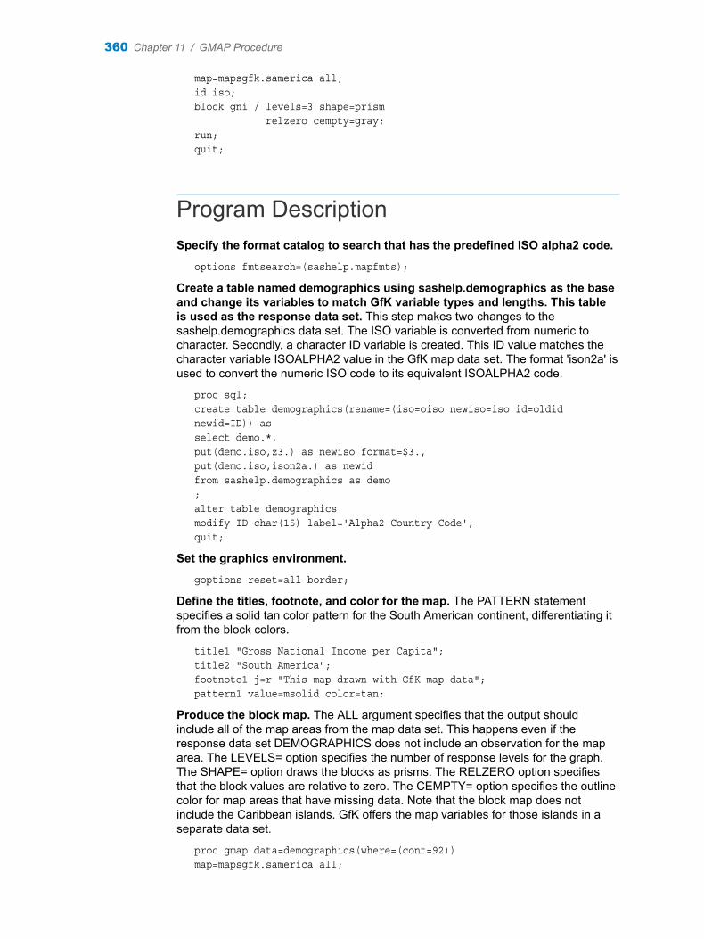
map=mapsgfk.samerica all;id iso;block gni / levels=3 shape=prism relzero cempty=gray;run;quit;
Program DescriptionSpecify the format catalog to search that has the predefined ISO alpha2 code.
options fmtsearch=(sashelp.mapfmts);
Create a table named demographics using sashelp.demographics as the base and change its variables to match GfK variable types and lengths. This table is used as the response data set. This step makes two changes to the sashelp.demographics data set. The ISO variable is converted from numeric to character. Secondly, a character ID variable is created. This ID value matches the character variable ISOALPHA2 value in the GfK map data set. The format 'ison2a' is used to convert the numeric ISO code to its equivalent ISOALPHA2 code.
proc sql;create table demographics(rename=(iso=oiso newiso=iso id=oldid newid=ID)) asselect demo.*, put(demo.iso,z3.) as newiso format=$3.,put(demo.iso,ison2a.) as newid from sashelp.demographics as demo;alter table demographicsmodify ID char(15) label='Alpha2 Country Code';quit;
Set the graphics environment.
goptions reset=all border;
Define the titles, footnote, and color for the map. The PATTERN statement specifies a solid tan color pattern for the South American continent, differentiating it from the block colors.
title1 "Gross National Income per Capita";title2 "South America";footnote1 j=r "This map drawn with GfK map data";pattern1 value=msolid color=tan;
Produce the block map. The ALL argument specifies that the output should include all of the map areas from the map data set. This happens even if the response data set DEMOGRAPHICS does not include an observation for the map area. The LEVELS= option specifies the number of response levels for the graph. The SHAPE= option draws the blocks as prisms. The RELZERO option specifies that the block values are relative to zero. The CEMPTY= option specifies the outline color for map areas that have missing data. Note that the block map does not include the Caribbean islands. GfK offers the map variables for those islands in a separate data set.
proc gmap data=demographics(where=(cont=92))map=mapsgfk.samerica all;
360 Chapter 11 / GMAP Procedure

id iso;block gni / levels=3 shape=prism relzero cempty=gray;run;quit;
Example 4: Using Traditional Map Data to Specify Response Levels in a Block MapFeatures: MAP= required argument referring to a traditional map data set
DATA= required argument referring to response dataID statementBLOCK statement options
LEVELS=SHAPE=RELZEROCEMPTY=
PATTERN statement
Data sets: MAPS.SAMERICA (map data set)SASHELP.DEMOGRAPHICS (response data)
Sample library member:
GMPLEVEL
Notes: The SAS Sample Library is not available in SAS Studio.You can download the mapping samples in the SAS Sample Library in zipped format from the SAS/GRAPH Learning and Support page on support.sas.com. Click the link for SAS/GRAPH and Base SAS: Mapping Reference (Examples ZIP).The map data set or data sets supplied by SAS and used in this program might not be an available resource on your system.
OutputThis example uses the LEVELS= option to specify the number of response levels for the blocks. The LEVELS= option tells GMAP how many response levels and the GMAP procedure calculates the quantiles.
Example 4: Using Traditional Map Data to Specify Response Levels in a Block Map361

Programgoptions reset=all border;
title1 "Gross National Income per Capita";title2 "South America";pattern1 value=msolid color=tan;
proc gmap data=sashelp.demographics(where=(cont=92)) map=maps.samerica all; id id; block gni / levels=3 shape=prism relzero cempty=gray;run;quit;
Program DescriptionSet the graphics environment.
goptions reset=all border;
Define the titles, footnote, and color for the map. The PATTERN statement specifies a solid tan color pattern for the South American continent, differentiating it from the block colors.
title1 "Gross National Income per Capita";title2 "South America";pattern1 value=msolid color=tan;
362 Chapter 11 / GMAP Procedure

Produce the block map, which includes the Caribbean islands. The ALL argument specifies that the output should include all of the map areas from the map data set. This happens even if the response data set DEMOGRAPHICS does not include an observation for the map area. The LEVELS= option specifies the number of response levels for the graph. The SHAPE= option draws the blocks as prisms. The RELZERO option specifies that the block values are relative to zero. The CEMPTY= option specifies the outline color for map areas that have missing data.
proc gmap data=sashelp.demographics(where=(cont=92)) map=maps.samerica all; id id; block gni / levels=3 shape=prism relzero cempty=gray;run;quit;
Example 5: Using GfK GeoMarketing Map Data to Assign a Format to the Response VariableFeatures: MAP= required argument referring to a GfK map data set
DATA= argument referring to response dataFORMAT statementID statementAREA statement option MIDPOINTS=BLOCK statement options
LEGEND=RELZEROLEVELS=
System option FMTSEARCH=SQL procedureFORMAT procedureLEGEND statementPATTERN statement
Data sets: MAPSGFK.ASIA (map data set)DEMOGRAPHICS (table of response data)
Format: ison2a
Restriction: The GfK GeoMarketing map data set used in this example is licensed to be used only with SAS/GRAPH.
Sample library member:
GMPGFRMT
Notes: The SAS Sample Library is not available in SAS Studio.You can download the mapping samples in the SAS Sample Library in zipped format from the SAS/GRAPH Learning and Support page on support.sas.com. Click the link for SAS/GRAPH and Base SAS: Mapping Reference (Examples ZIP).The map data set or data sets supplied by SAS and used in this program might not be an available resource on your system.
Example 5: Using GfK GeoMarketing Map Data to Assign a Format to the Response Variable 363

The ISO codes that are in the sashelp.demographics data set are not as recent as the ISO codes found in the MAPSGFK data set.
OutputThis example creates formats for the response variables. The format for the POP variable defines and labels ranges of values. These ranges appear in the legend and make the map easier to understand. The example also uses the AREA statement to patterns the map areas by region. The elongated countries in the output indicate that a different projection method was used with this GfK map than was used with the traditional Asia map data set.
Programoptions fmtsearch=(sashelp.mapfmts);
proc sql;create table demographics(rename=(iso=oiso newiso=iso id=oldid newid=ID)) asselect demo.*, put(demo.iso,z3.) as newiso format=$3.,put(demo.iso,ison2a.) as newid from sashelp.demographics as demo;alter table demographicsmodify ID char(15) label='Alpha2 Country Code';
364 Chapter 11 / GMAP Procedure

quit;
goptions reset=all border;
proc format; value popfmt low-1000000="0-1" 1000001-10000000="1-10" 10000001-100000000="10-100" 100000001-500000000="100-500" 500000001-high="over 500";run;
proc format; value $ regionfmt "SEAR" = "South-East Asia" "EUR" = "Europe" "EMR" = "Eastern Mediterranean" "WPR" = "Western Pacific";run;
title1 "Population Data for Asia (2005)";footnote j=r "This map drawn with GfK map data";pattern1 color=gold value=msolid;pattern2 color=yellow value=msolid;pattern3 color=cyan value=msolid;pattern4 color=light_blue value=msolid;
legend1 label=("Population (Millions)");
proc gmap data=demographics(where=(cont=95))map=mapsgfk.asia all;format pop popfmt.;format region $regionfmt.;id id;area region / midpoints="SEAR" "EUR" "EMR" "WPR";block pop / legend=legend1 relzero levels=all;run;quit;
Program DescriptionSpecify the format catalog to search that has the predefined ISO alpha2 code.
options fmtsearch=(sashelp.mapfmts);
Create a table named demographics using sashelp.demographics as the base and change its variables to match GfK variable types and lengths. This table is used as the response data set. This step makes two changes to the sashelp.demographics data set. The ISO variable is converted from numeric to character. Secondly, a character ID variable is created. This ID value matches the character variable ISOALPHA2 value in the GfK map data set. The format 'ison2a' is used to convert the numeric ISO code to its equivalent ISOALPHA2 code.
proc sql;create table demographics(rename=(iso=oiso newiso=iso id=oldid newid=ID)) asselect demo.*,
Example 5: Using GfK GeoMarketing Map Data to Assign a Format to the Response Variable 365

put(demo.iso,z3.) as newiso format=$3.,put(demo.iso,ison2a.) as newid from sashelp.demographics as demo;alter table demographicsmodify ID char(15) label='Alpha2 Country Code';quit;
Set the graphics environment.
goptions reset=all border;
Create a format for the POP variable. POPFMT. defines the ranges of values for POP and labels the values.
proc format; value popfmt low-1000000="0-1" 1000001-10000000="1-10" 10000001-100000000="10-100" 100000001-500000000="100-500" 500000001-high="over 500";run;
Create a format for the REGION variable. REGIONFMT. labels the values for REGION.
proc format; value $ regionfmt "SEAR" = "South-East Asia" "EUR" = "Europe" "EMR" = "Eastern Mediterranean" "WPR" = "Western Pacific";run;
Define the title, footnote, and colors for the map. The PATTERN statement specifies a unique solid color pattern for each country of the Asian continent, differentiating it from the block colors.
title1 "Population Data for Asia (2005)";footnote j=r "This map drawn with GfK map data";pattern1 color=gold value=msolid;pattern2 color=yellow value=msolid;pattern3 color=cyan value=msolid;pattern4 color=light_blue value=msolid;
Assign the legend label.
legend1 label=("Population (Millions)");
Produce the block map. The ALL argument specifies that the map displayed should include all of the map areas from the map data set. This happens even if the response data set DEMOGRAPHICS does not include an observation for the map area. The map displayed shows one such area. The FORMAT statements assign POPFMT. to the POP variable and $REGIONFMT. to the REGION variable. The ID statement assigns the variable ID—which represents the ISOALPHA2 variable after the variable rename when the demographics table was set up. The AREA statement assigns patterns to the map areas according to the values of the REGION variable. The RELZERO option specifies that the blocks values are relative to zero. The LEVELS= option is used to graph all unique ID response variable values.
proc gmap data=demographics(where=(cont=95))map=mapsgfk.asia all;format pop popfmt.;
366 Chapter 11 / GMAP Procedure

format region $regionfmt.;id id;area region / midpoints="SEAR" "EUR" "EMR" "WPR";block pop / legend=legend1 relzero levels=all;run;quit;
Example 6: Using Traditional Map Data to Assign a Format to the Response VariableFeatures: MAP= required argument referring to a traditional map data set
DATA= required argument referring to response dataFORMAT statementID statementAREA statement option MIDPOINTS=BLOCK statement options
LEGEND=RELZERO
FORMAT procedureLEGEND statementPATTERN statement
Data sets: MAPS.ASIA (map data set)SASHELP.DEMOGRAPHICS (response data)
Sample library member:
GMPFORMT
Notes: The SAS Sample Library is not available in SAS Studio.You can download the mapping samples in the SAS Sample Library in zipped format from the SAS/GRAPH Learning and Support page on support.sas.com. Click the link for SAS/GRAPH and Base SAS: Mapping Reference (Examples ZIP).The map data set or data sets supplied by SAS and used in this program might not be an available resource on your system.
OutputThis example creates formats for the response variables. The format for the POP variable defines and labels ranges of values. These ranges appear in the legend and make the map easier to understand. The example also uses the AREA statement to patterns the map areas by region.
Example 6: Using Traditional Map Data to Assign a Format to the Response Variable367

Programgoptions reset=all border;
proc format; value popfmt low-1000000="0-1" 1000001-10000000="1-10" 10000001-100000000="10-100" 100000001-500000000="100-500" 500000001-high="over 500";run;
proc format; value $ regionfmt "SEAR" = "South-East Asia" "EUR" = "Europe" "EMR" = "Eastern Mediterranean" "WPR" = "Western Pacific";run;
title1 "Population Data for Asia (2005)";pattern1 color=gold value=msolid;pattern2 color=yellow value=msolid;pattern3 color=cyan value=msolid;pattern4 color=light_blue value=msolid;
legend1 label=("Population (Millions)");
proc gmap data=sashelp.demographics(where=(cont=95)) map=maps.asia all; format pop popfmt.; format region $regionfmt.; id id;
368 Chapter 11 / GMAP Procedure

area region / midpoints="SEAR" "EUR" "EMR" "WPR"; block pop / legend=legend1 relzero levels=all;run;quit;
Program DescriptionSet the graphics environment.
goptions reset=all border;
Create a format for POP. POPFMT. defines the ranges of values for POP and labels the values.
proc format; value popfmt low-1000000="0-1" 1000001-10000000="1-10" 10000001-100000000="10-100" 100000001-500000000="100-500" 500000001-high="over 500";run;
Create a format for REGION. REGIONFMT. labels the values for REGION.
proc format; value $ regionfmt "SEAR" = "South-East Asia" "EUR" = "Europe" "EMR" = "Eastern Mediterranean" "WPR" = "Western Pacific";run;
Define the title and colors for the map. The PATTERN statement specifies a unique solid color pattern for each country of the Asian continent, differentiating it from the block colors.
title1 "Population Data for Asia (2005)";pattern1 color=gold value=msolid;pattern2 color=yellow value=msolid;pattern3 color=cyan value=msolid;pattern4 color=light_blue value=msolid;
Assign the legend label.
legend1 label=("Population (Millions)");
Produce the block maps. The ALL argument specifies that the map displayed should include all of the map areas from the map data set. This happens even if the response data set DEMOGRAPHICS does not include an observation for the map area. The FORMAT statements assign POPFMT. to the POP variable and $REGIONFMT. to the REGION variable. The AREA statement assigns patterns to the map areas according to the values of the REGION variable. The RELZERO option specifies that the blocks values are relative to zero. The LEVELS= option is used to graph all unique ID response variable values.
proc gmap data=sashelp.demographics(where=(cont=95)) map=maps.asia all; format pop popfmt.;
Example 6: Using Traditional Map Data to Assign a Format to the Response Variable369

format region $regionfmt.; id id; area region / midpoints="SEAR" "EUR" "EMR" "WPR"; block pop / legend=legend1 relzero levels=all;run;quit;
Example 7: Using GfK GeoMarketing Map Data When Specifying the Statistic for the Response VariableFeatures: MAP= required argument referring to a GfK map data set
DATA= required argument referring to response dataID statementBLOCK statement options
STATISTIC=LEVELS=RELZERO
PATTERN statement
Data sets: MAPSGFK.US (map data set)SASHELP.ZIPCODE (response data)
Restriction: The GfK GeoMarketing map data set used in this example is licensed to be used only with SAS/GRAPH.
Sample library member:
GMPGSTAT
Notes: The SAS Sample Library is not available in SAS Studio.You can download the mapping samples in the SAS Sample Library in zipped format from the SAS/GRAPH Learning and Support page on support.sas.com. Click the link for SAS/GRAPH and Base SAS: Mapping Reference (Examples ZIP).The map data set or data sets supplied by SAS and used in this program might not be an available resource on your system.
OutputThis example specifies the statistic for the response variable that is displayed by the block map. The STATISTIC= option specifies that the statistic is frequency rather than the default statistic (sum).
370 Chapter 11 / GMAP Procedure

Programgoptions reset=all border;
title1 "Number of ZIP Codes per State";footnote j=r "This map drawn with GfK map data";pattern1 value=msolid color=tan;
proc gmap map=mapsgfk.us data=sashelp.zipcode all;id state;block zip / statistic=frequency levels=5 relzero;run;quit;
Program DescriptionSet the graphics environment.
goptions reset=all border;
Define the title, footnote, and color for the map.
title1 "Number of ZIP Codes per State";footnote j=r "This map drawn with GfK map data";pattern1 value=msolid color=tan;
Produce the block maps. The ALL argument specifies that the map displayed should include all of the map areas from the map data set. This happens even if the
Example 7: Using GfK GeoMarketing Map Data When Specifying the Statistic for the Response Variable 371

response data set SASHELP.ZIPCODE does not include an observation for the map area. The STATISTIC= option specifies the statistic for the response variable. The LEVELS= option specifies the number of response levels. The RELZERO option specifies that the blocks values are relative to zero. Note that the MAPSGFK.US map data set does not include Puerto Rico or the District of Columbia. Block maps created with the traditional MAPS.US map data set include these map areas.
proc gmap map=mapsgfk.us data=sashelp.zipcode all;id state;block zip / statistic=frequency levels=5 relzero;run;quit;
Example 8: Using Traditional Map Data When Specifying the Statistic for the Response VariableFeatures: MAP= required argument referring to a traditional map data set
DATA= required argument referring to response dataID statementBLOCK statement options
STATISTIC=LEVELS=RELZERO
PATTERN statement
Data sets: MAPS.US (map data set)SASHELP.ZIPCODE (response data)
Sample library member:
GMPSTAT
Notes: The SAS Sample Library is not available in SAS Studio.You can download the mapping samples in the SAS Sample Library in zipped format from the SAS/GRAPH Learning and Support page on support.sas.com. Click the link for SAS/GRAPH and Base SAS: Mapping Reference (Examples ZIP).The map data set or data sets supplied by SAS and used in this program might not be an available resource on your system.
OutputThis example specifies the statistic for the response variable that is displayed by the block map. The STATISTIC= option specifies that the statistic is frequency rather than the default statistic (sum).
372 Chapter 11 / GMAP Procedure
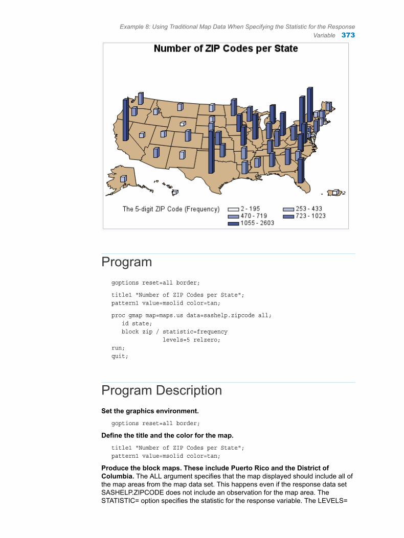
Programgoptions reset=all border;
title1 "Number of ZIP Codes per State";pattern1 value=msolid color=tan;
proc gmap map=maps.us data=sashelp.zipcode all; id state; block zip / statistic=frequency levels=5 relzero;run;quit;
Program DescriptionSet the graphics environment.
goptions reset=all border;
Define the title and the color for the map.
title1 "Number of ZIP Codes per State";pattern1 value=msolid color=tan;
Produce the block maps. These include Puerto Rico and the District of Columbia. The ALL argument specifies that the map displayed should include all of the map areas from the map data set. This happens even if the response data set SASHELP.ZIPCODE does not include an observation for the map area. The STATISTIC= option specifies the statistic for the response variable. The LEVELS=
Example 8: Using Traditional Map Data When Specifying the Statistic for the Response Variable 373

option specifies the number of response levels. The RELZERO option specifies that the blocks values are relative to zero.
proc gmap map=maps.us data=sashelp.zipcode all; id state; block zip / statistic=frequency levels=5 relzero;run;quit;
Example 9: Using GfK GeoMarketing Map Data to Produce a Simple Choropleth MapFeatures: MAP= required argument referring to a GfK map data set
DATA= argument referring to response dataID statementCHORO statement options
STAT=CDEFAULT=
System option FMTSEARCH=SQL procedure
Data sets: MAPSGFK.EUROPE (map data set)DEMOGRAPHICS (table of response data)
Format: ison2a
Restriction: The GfK GeoMarketing map data set used in this example is licensed to be used only with SAS/GRAPH.
Sample library member:
GMPGCHOR
Notes: The SAS Sample Library is not available in SAS Studio.You can download the mapping samples in the SAS Sample Library in zipped format from the SAS/GRAPH Learning and Support page on support.sas.com. Click the link for SAS/GRAPH and Base SAS: Mapping Reference (Examples ZIP).The map data set or data sets supplied by SAS and used in this program might not be an available resource on your system.The ISO codes that are in the sashelp.demographics data set are not as recent as the ISO codes found in the MAPSGFK data set.
OutputThis example produces a choropleth (two-dimensional) map that shows the population of countries in Europe. Because the DISCRETE option is not used, the response variable is assumed to have a continuous range of values. Because neither the LEVELS= nor MIDPOINTS= options are used, the GMAP procedure selects a number of levels based on the number of map areas. It then calculates the appropriate response levels. The legend shows the range of values for each level.
374 Chapter 11 / GMAP Procedure

Programoptions fmtsearch=(sashelp.mapfmts);
proc sql;create table demographics(rename=(iso=oiso newiso=iso id=oldid newid=ID)) asselect demo.*, put(demo.iso,z3.) as newiso format=$3.,put(demo.iso,ison2a.) as newid from sashelp.demographics as demo;alter table demographicsmodify ID char(15) label='Alpha2 Country Code';quit;
goptions reset=all border;
title1 "Population in Europe";footnote j=r "This map drawn with GfK map data";
proc gmap map=mapsgfk.europe(where=(id not in:('SJ' 'TR'))) data=demographics(where=(cont=93)) all;id id;choro pop / cdefault=yellow stat=first;run;quit;
Example 9: Using GfK GeoMarketing Map Data to Produce a Simple Choropleth Map375

Program DescriptionSpecify the format catalog to search that has the predefined ISO alpha2 code.
options fmtsearch=(sashelp.mapfmts);
Create a table named demographics using sashelp.demographics as the base and change its variables to match GfK variable types and lengths. This table is used as the response data set. This step makes two changes to the sashelp.demographics data set. The ISO variable is converted from numeric to character. Secondly, a character ID variable is created. This ID value matches the character variable ISOALPHA2 value in the GfK map data set. The format 'ison2a' is used to convert the numeric ISO code to its equivalent ISOALPHA2 code.
proc sql;create table demographics(rename=(iso=oiso newiso=iso id=oldid newid=ID)) asselect demo.*, put(demo.iso,z3.) as newiso format=$3.,put(demo.iso,ison2a.) as newid from sashelp.demographics as demo;alter table demographicsmodify ID char(15) label='Alpha2 Country Code';quit;
Set the graphics environment.
goptions reset=all border;
Define the title and the footnote for the map.
title1 "Population in Europe";footnote j=r "This map drawn with GfK map data";
Produce the choropleth map. The ALL argument specifies that the output should include all of the map areas from the map data set. This happens even if the response data set DEMOGRAPHICS does not include an observation for the map area. The output shows three such areas. The ID statement specifies the variable that is in both the map data set and the response data set that defines map areas. CDEFAULT= specifies the color for the map areas that have missing data. In this map Montenegro, Kosovo, and the island of Cyprus are yellow, indicating missing data. The STATISTIC= option specifies that the GMAP procedure is to match the first observation from MAPSGFK.EUROPE data set and display the response value from this observation only. The WHERE= data set option on the MAP= option excludes the islands of Svalbard, the country Turkey and Jan Mayen Islands, and these map areas have no data in the DEMOGRAPHICS data set. The data set MAPSGFK.EUROPE does not contain the Russian countries of Azerbaijan, Armenia and Georgia, and therefore these countries are not shown in the map.
proc gmap map=mapsgfk.europe(where=(id not in:('SJ' 'TR'))) data=demographics(where=(cont=93)) all;id id;choro pop / cdefault=yellow stat=first;run;quit;
376 Chapter 11 / GMAP Procedure

Example 10: Using Traditional Map Data to Produce a Simple Choropleth MapFeatures: MAP= required argument referring to a traditional map data set
DATA= required argument referring to response dataID statementCHORO statement option CDEFAULT=
Data sets: MAPS.EUROPE (map data set)SASHELP.DEMOGRAPHICS (response data)
Sample library member:
GMPCHORO
Notes: The SAS Sample Library is not available in SAS Studio.You can download the mapping samples in the SAS Sample Library in zipped format from the SAS/GRAPH Learning and Support page on support.sas.com. Click the link for SAS/GRAPH and Base SAS: Mapping Reference (Examples ZIP).The map data set or data sets supplied by SAS and used in this program might not be an available resource on your system.
OutputThis example produces a choropleth (two-dimensional) map that shows the population of countries in Europe. Because the DISCRETE option is not used, the response variable is assumed to have a continuous range of values. Because neither the LEVELS= nor MIDPOINTS= options are used, the GMAP procedure selects a number of levels based on the number of map areas. It then calculates the appropriate response levels. The legend shows the range of values for each level.
Example 10: Using Traditional Map Data to Produce a Simple Choropleth Map 377

Programgoptions reset=all border;
title1 "Population in Europe";
proc gmap map=maps.europe(where=(id ne 405 and id ne 845)) data=sashelp.demographics(where=(cont=93)) all; id id; choro pop / cdefault=yellow;run;quit;
Program DescriptionSet the graphics environment.
goptions reset=all border;
Define the title for the map.
title1 "Population in Europe";
Produce the choropleth map. The ALL argument specifies that the map displayed should include all of the map areas from the map data set. This happens even if the response data set DEMOGRAPHICS does not include an observation for the map area. The map shows one such area. The ID statement specifies the variable that is in both the map data set and the response data set that defines map areas. CDEFAULT= specifies the color for the map areas that have missing data. The WHERE= data set option on the MAP= option excludes the islands of Greenland
378 Chapter 11 / GMAP Procedure

and Svalbard, which have no data in DEMOGRAPHICS data set. The data sets MAPS.EUROPE and SASHELP.DEMOGRAPHICS include the Russian region countries Azerbaijan, Armenia, and Georgia.
proc gmap map=maps.europe(where=(id ne 405 and id ne 845)) data=sashelp.demographics(where=(cont=93)) all; id id; choro pop / cdefault=yellow;run;quit;
Example 11: Using Traditional Map Data to Produce a Drilldown Choropleth MapFeatures: MAP= required argument referring to a traditional map data set
DATA= required argument referring to response dataBY statementID statementCHORO statement options
LEVELS=NOLEGENDCOUTLINE=HTML=DES=NAME=
Data sets: MAPSSAS.US (map data set)MYDATA (response data)
Sample library member:
GMPCHORD
Notes: The SAS Sample Library is not available in SAS Studio.You can download the mapping samples in the SAS Sample Library in zipped format from the SAS/GRAPH Learning and Support page on support.sas.com. Click the link for SAS/GRAPH and Base SAS: Mapping Reference (Examples ZIP).The map data set or data sets supplied by SAS and used in this program might not be an available resource on your system.
OutputThis example produces three choropleth (two-dimensional) maps, each showing the population of a southeastern state in America. Each graph’s title includes a link for drilling down to that particular state’s home page on the web. The ‘ALT=’ option text description on each map title changes with a BY variable substitution to match the state being highlighted. The LEVELS= option enables the GMAP procedure to graph one response level for the population. This population number is part of the text description as your mouse pointer is held over the state colored in blue.
Example 11: Using Traditional Map Data to Produce a Drilldown Choropleth Map 379

380 Chapter 11 / GMAP Procedure

Program%let name=map001;filename odsout '.';
data mydata;format population comma12.0;input statecode $ 1-2 population;year=2000;statename=fipnamel(stfips(statecode));datalines;VA 7078515NC 8049313SC 4012012;run;
proc sort data=mydata out=mydata;by statecode statename;run;
data mydata; set mydata;length htmlvar $500;htmlvar='title='||quote( 'State: '|| trim(left(statename)) ||'0D'x|| 'Population: '|| trim(left(put(population,comma12.0))) )|| ' href="https://www.state.'||trim(left(lowcase(statecode)))||'.us"';run;
goptions device=png gunit=pct htitle=6 htext=4 border;
Example 11: Using Traditional Map Data to Produce a Drilldown Choropleth Map 381

ods _all_ close;ods html path=odsout body="&name..htm" (title="SAS/Graph ODS HTML Drilldown Map") style=sasweb;
axis1 label=none;axis2 label=none minor=none offset=(0,0);
pattern v=solid color=cx43a2ca;
options nobyline;title1 "Drilldown Map for " color=blue underlin=1 link="https://www.state.#byval(statecode)..us" alt="Click to drilldown to #byval(statename) home page" "#byval(statename)";
proc gmap data=mydata map=mapssas.us all; by statecode statename;id statecode;choro population / levels=1 nolegend coutline=black html=htmlvar des='' name="&name._#byval(statecode)"; run;quit;
ods html close;ods html;
Program DescriptionSet up the output filename.
%let name=map001;filename odsout '.';
Create the response data set MYDATA with the U.S. states to map.
data mydata;format population comma12.0;input statecode $ 1-2 population;year=2000;statename=fipnamel(stfips(statecode));datalines;VA 7078515NC 8049313SC 4012012;run;
Sort the response data.
proc sort data=mydata out=mydata;by statecode statename;run;
Set up the text when holding your mouse pointer over a highlighted state.
382 Chapter 11 / GMAP Procedure

data mydata; set mydata;length htmlvar $500;htmlvar='title='||quote( 'State: '|| trim(left(statename)) ||'0D'x|| 'Population: '|| trim(left(put(population,comma12.0))) )|| ' href="https://www.state.'||trim(left(lowcase(statecode)))||'.us"';run;
Set the graphics environment. The following ODS statements close all previously open destinations and store PNG output in your working directory. From there you can open the file in a web browser.
goptions device=png gunit=pct htitle=6 htext=4 border;ods _all_ close;ods html path=odsout body="&name..htm" (title="SAS/Graph ODS HTML Drilldown Map") style=sasweb;
Suppress the axis labels.
axis1 label=none;axis2 label=none minor=none offset=(0,0);
Set the color to highlight the state.
pattern v=solid color=cx43a2ca;
Define the title and its drilldown link for the map. NOBYLINE suppresses the output of both BY variables indicated in the BY statement. The individual BY variables are used in the LINK= and ALT= option specifications. #BYVAL substitutes the current value of the BY variable, (statecode) or (statename), for #BYVAL in the text string and displays it.
options nobyline;title1 "Drilldown Map for " color=blue underlin=1 link="https://www.state.#byval(statecode)..us" alt="Click to drilldown to #byval(statename) home page" "#byval(statename)";
Produce the choropleth map. for each state. The BY statement specifies the variables in the response data set to work with. The ID statement specifies the FIPS state code variable that is in both the map data set and the response data set that defines map areas. The LEVELS= option enables the GMAP procedure to graph one response level for the population. COUTLINE= specifies that the map area be outlined in black. HTML= sets up the link that is displayed as your mouse pointer is held over the state in the output. NAME= defines the name of the GRSEG catalog entry and the name of the graphics output file.
proc gmap data=mydata map=mapssas.us all; by statecode statename;id statecode;choro population / levels=1 nolegend coutline=black html=htmlvar des='' name="&name._#byval(statecode)"; run;quit;
Example 11: Using Traditional Map Data to Produce a Drilldown Choropleth Map 383

Reset the graphics environment. Run ODS HTML to close the output file, and then reopen ODS HTML. Reopening the HTML destination is not required when running the code in SAS Studio.
ods html close;ods html;
Example 12: Using GfK GeoMarketing Map Data When Labeling Provinces on a MapFeatures: MAP= required argument referring to a GfK map data set
DATA= required argument referring to response dataID statementCHORO statement options
ANNOTATE=NOLEGENDCOUTLINE=STAT=
GREMOVE procedureSORT procedureAnnotate Facility
Data set: MAPSGFK.BELARUS (map data set)
Restriction: The GfK GeoMarketing map data set used in this example is licensed to be used only with SAS/GRAPH.
Sample library member:
GMPGLABL
Notes: The SAS Sample Library is not available in SAS Studio.You can download the mapping samples in the SAS Sample Library in zipped format from the SAS/GRAPH Learning and Support page on support.sas.com. Click the link for SAS/GRAPH and Base SAS: Mapping Reference (Examples ZIP).The map data set or data sets supplied by SAS and used in this program might not be an available resource on your system.
OutputThis example uses the Annotate facility to add labels to each area in a map of Belarus. The CHORO statement assigns the Annotate data set to the map. The %MAPLABEL Annotate macro is used to create and position the map labels. For more information about this macro, see “%MAPLABEL Annotate Macro” in SAS/GRAPH: Reference.
384 Chapter 11 / GMAP Procedure

Programgoptions reset=all border;
title "Labeling Provinces with the MAPLABEL Macro";footnote j=r "This map drawn with GfK map data";
proc sort data=mapsgfk.belarus out=belarus;by id1 id; run;
proc gremove data=belarus out=belarus_outline;by id1;id id;run;
%annomac;%maplabel (belarus_outline, mapsgfk.belarus_attr, work.labelout, id1name, id1, font=Albany AMT, color=black, size=2.5, hsys=3);
proc gmap map=belarus data=belarus; id id1 id; choro id1 / nolegend annotate=labelout coutline=gray stat=first;run;quit;
Example 12: Using GfK GeoMarketing Map Data When Labeling Provinces on a Map385

Program DescriptionSet the graphics environment.
goptions reset=all border;
Define the title and the footnote for the map.
title "Labeling Provinces with the MAPLABEL Macro";footnote j=r "This map drawn with GfK map data";
Sort the GfK data by region and district variables.
proc sort data=mapsgfk.belarus out=belarus;by id1 id; run;
Use the GREMOVE procedure to remove the internal boundaries from the Belarus map. The output data set from GREMOVE is used by the %MAPLABEL macro to determine the centroid of each province for positioning the province label.
proc gremove data=belarus out=belarus_outline;by id1;id id;run;
Create the Annotate data set. The %ANNOMAC macro enables the Annotate macros. The %MAPLABEL macro calculates the centroid and creates the Annotate data set.
%annomac;%maplabel (belarus_outline, mapsgfk.belarus_attr, work.labelout, id1name, id1, font=Albany AMT, color=black, size=2.5, hsys=3);
Produce the choropleth map. The NOLEGEND option suppresses the legend. The ANNOTATE= option specifies the data set to annotate the map. The COUTLINE= option outlines each province in gray. The STATISTIC= option specifies that the GMAP procedure match the first observation from the BELARUS data set and display the response value from this observation only.
proc gmap map=belarus data=belarus; id id1 id; choro id1 / nolegend annotate=labelout coutline=gray stat=first;run;quit;
Example 13: Using Traditional Map Data When Labeling Provinces on a MapFeatures: MAP= required argument referring to a traditional map data set
DATA= required argument referring to response dataID statementCHORO statement options
STAT=ANNOTATE=
386 Chapter 11 / GMAP Procedure

NOLEGENDThe global PATTERN statementAnnotate Facility
Data set: MAPS.BELARUS (map data set)
Sample library member:
GMPLABEL
Notes: The SAS Sample Library is not available in SAS Studio.You can download the mapping samples in the SAS Sample Library in zipped format from the SAS/GRAPH Learning and Support page on support.sas.com. Click the link for SAS/GRAPH and Base SAS: Mapping Reference (Examples ZIP).The map data set or data sets supplied by SAS and used in this program might not be an available resource on your system.
OutputThis example uses the Annotate facility to add labels to each area in a map of Belarus. The CHORO statement assigns the Annotate data set to the map. The %MAPLABEL Annotate macro is used to create and position the map labels. For more information about this macro, see “%MAPLABEL Annotate Macro” in SAS/GRAPH: Reference.
Example 13: Using Traditional Map Data When Labeling Provinces on a Map 387

Programgoptions reset=all border;
title "Labeling Provinces with the MAPLABEL Macro";
pattern1 value=empty color=blue repeat=6;
%annomac;%maplabel (maps.belarus, maps.belarus2, work.labelout, idname, id, font=Arial Black, color=crimson, size=4, hsys=3);
proc gmap map=maps.belarus data=maps.belarus; id id; choro id / stat=sum nolegend annotate=labelout;run;quit;
Program DescriptionSet the graphics environment.
goptions reset=all border;
Define the title for the map.
title "Labeling Provinces with the MAPLABEL Macro";
Define pattern characteristics. PATTERN1 defines a single map pattern that is repeated for each of the six map areas (provinces). The pattern is an empty fill with a blue border. The VALUE= option defines a map or plot pattern. Specifying a color causes PATTERN1 to generate only one pattern definition. The REPEAT= option specifies the number of times to repeat the pattern definition.
pattern1 value=empty color=blue repeat=6;
Create the Annotate data set. The %ANNOMAC macro enables the Annotate macros. The %MAPLABEL macro calculates the centroid and creates the Annotate data set.
%annomac;%maplabel (maps.belarus, maps.belarus2, work.labelout, idname, id, font=Arial Black, color=crimson, size=4, hsys=3);
Produce the choropleth map. Use the option STATISTIC=SUM to chart the summed value of all observations with a given matching ID. The NOLEGEND option suppresses the legend. The ANNOTATE= option specifies the data set to annotate the map.
proc gmap map=maps.belarus data=maps.belarus; id id; choro id / stat=sum nolegend annotate=labelout;run;quit;
388 Chapter 11 / GMAP Procedure

Example 14: Combining Traditional Map Data and Sample Response Data to Map U.S. Population StatisticsFeatures: MAP= required argument referring to a traditional map data set
DATA= required argument referring to response data in a sample data setID statementCHORO statement options
LEVELS=LEGEND=
Data sets: MAPSSAS.US (map data set)SASHELP.US_DATA (response data)
Sample library member:
GMPUSDAT
Notes: The SAS Sample Library is not available in SAS Studio.You can download the mapping samples in the SAS Sample Library in zipped format from the SAS/GRAPH Learning and Support page on support.sas.com. Click the link for SAS/GRAPH and Base SAS: Mapping Reference (Examples ZIP).The map data set or data sets supplied by SAS and used in this program might not be an available resource on your system.
OutputThis example uses a sample response data set named SASHELP.US_DATA that is specifically designed to be used with the traditional map data set MAPS.US or MAPSSAS.US. In this example, population details per state are mapped.
Example 14: Combining Traditional Map Data and Sample Response Data to Map U.S. Population Statistics 389

Programgoptions reset=all border;
title1 ls=1.5 "Using Sample U.S. Response Data";
legend1 label=(position=top) shape=bar(.1in,.1in);
proc gmap data=sashelp.us_data map=mapssas.us;id state;choro density_2010 / levels=3 legend=legend1;run;quit;
Program DescriptionSet the graphics environment.
goptions reset=all border;
Define the title for the map.
title1 ls=1.5 "Using Sample U.S. Response Data";
Define the legend for the map.
legend1 label=(position=top) shape=bar(.1in,.1in);
Produce the choropleth map of the United States. 2020 population densities are mapped per state. Use the sample response data set SASHELP.US_DATA, and the
390 Chapter 11 / GMAP Procedure

traditional map data set for the United States. The LEVELS= option specifies that 3 ranges of population values from the response data are graphed.
proc gmap data=sashelp.us_data map=mapssas.us;id state;choro density_2010 / levels=3 legend=legend1;run;quit;
Example 15: Using GfK GeoMarketing Map Data to Produce a Simple Prism MapFeatures: MAP= required argument referring to a GfK map data set
DATA= argument referring to response dataID statementPRISM statement options
CDEFAULT=RELZERO
System option FMTSEARCH=SQL procedure
Data sets: MAPSGFK.AFRICA (map data set)DEMOGRAPHICS (table of response data)
Format: ison2a
Restriction: The GfK GeoMarketing map data set used in this example is licensed to be used only with SAS/GRAPH.
Sample library member:
GMPGPRSM
Notes: The SAS Sample Library is not available in SAS Studio.You can download the mapping samples in the SAS Sample Library in zipped format from the SAS/GRAPH Learning and Support page on support.sas.com. Click the link for SAS/GRAPH and Base SAS: Mapping Reference (Examples ZIP).The map data set or data sets supplied by SAS and used in this program might not be an available resource on your system.
Example 15: Using GfK GeoMarketing Map Data to Produce a Simple Prism Map 391

Output
Programoptions fmtsearch=(sashelp.mapfmts);
proc sql;create table demographics(rename=(iso=oiso newiso=iso id=oldid newid=ID)) asselect demo.*, put(demo.iso,z3.) as newiso format=$3.,put(demo.iso,ison2a.) as newid from sashelp.demographics as demo;alter table demographicsmodify ID char(15) label='Alpha2 Country Code';quit;
goptions reset=all border;
title1 "Population in Africa";footnote1 j=r "This map drawn with GfK map data";
proc gmap data=demographics(where=(cont=94)) map=mapsgfk.africa(where=(lake=0)) density=low all; id id; prism pop / cdefault=yellow relzero;run;quit;
392 Chapter 11 / GMAP Procedure

Program DescriptionSpecify the format catalog to search that has the predefined ISO alpha2 code.
options fmtsearch=(sashelp.mapfmts);
Create a table named demographics using sashelp.demographics as the base and changing its variables to match GfK variable types and lengths. This table is used as the response data set. Note that the ISO variable was numeric in the original sashelp.demographics data but is the character variable OISO in the GfK map data set. The format 'ison2a' uses the country's ISO numeric code to display the country's ISO alpha2 code. Also note that the ID variable was a numeric geographic locator code (glc) in the original sashelp.demographics data. However, it is represented by the ISOALPHA2 variable in the GfK map data set.
proc sql;create table demographics(rename=(iso=oiso newiso=iso id=oldid newid=ID)) asselect demo.*, put(demo.iso,z3.) as newiso format=$3.,put(demo.iso,ison2a.) as newid from sashelp.demographics as demo;alter table demographicsmodify ID char(15) label='Alpha2 Country Code';quit;
Set the graphics environment.
goptions reset=all border;
Define the title and footnote for the map
title1 "Population in Africa";footnote1 j=r "This map drawn with GfK map data";
Produce the prism map. The WHERE= data set option in the DATA= statement includes the countries that are part of the continent of Africa. The WHERE= data set option in the MAP= statement excludes lake areas. The ALL argument specifies that the map displayed should include all of the map areas from the map data set. This happens even if the response data set DEMOGRAPHICS does not include an observation for the map area. The map shows one such area. The ID statement specifies the variable in the map data set and the response data set that defines map areas. The CDEFAULT= option sets the color of map areas that have missing data. The RELZERO option makes the prism heights relative to zero.
proc gmap data=demographics(where=(cont=94)) map=mapsgfk.africa(where=(lake=0)) density=low all; id id; prism pop / cdefault=yellow relzero;run;quit;
Example 15: Using GfK GeoMarketing Map Data to Produce a Simple Prism Map 393

Example 16: Using Traditional Map Data to Produce a Simple Prism MapFeatures: MAP= required argument referring to a traditional map data set
DATA= required argument referring to response dataID statementPRISM statement options
CDEFAULT=RELZERO
SAS DATA step with assignment statements
Data sets: MAPS.AFRICA (map data set)SASHELP.DEMOGRAPHICS (response data)
Sample library member:
GMPPRISM
Notes: The SAS Sample Library is not available in SAS Studio.You can download the mapping samples in the SAS Sample Library in zipped format from the SAS/GRAPH Learning and Support page on support.sas.com. Click the link for SAS/GRAPH and Base SAS: Mapping Reference (Examples ZIP).The map data set or data sets supplied by SAS and used in this program might not be an available resource on your system.
This example produces a prism map of the population of countries in Africa. Because the DISCRETE option is not used, the response variable is assumed to have a continuous range of values. Because neither the LEVELS= nor MIDPOINTS= option is used, the GMAP procedure selects a number of levels based on the number of map areas. It then calculates the appropriate response levels.
Because the XVIEW=, YVIEW=, and ZVIEW= options are not used, the default viewing position, above and to the east and south of the center of the map, is used. Because the XLIGHT= and YLIGHT= options are not used, none of the side polygons of the prisms are shadowed. The light source is the same as the viewing position.
394 Chapter 11 / GMAP Procedure

Output
Programgoptions reset=all border;
title1 "Population in Africa";
data africa;set maps.africa;by id segment;if first.id then lake=0;if x=. then lake+1;retain lake;run;
proc gmap data=sashelp.demographics(where=(cont=94)) map=africa(where=(lake=0)) density=low all; id id; prism pop / cdefault=yellow relzero;run;quit;
Program DescriptionSet the graphics environment.
Example 16: Using Traditional Map Data to Produce a Simple Prism Map 395
goptions reset=all border;
Define the title for the map.
title1 "Population in Africa";
Identify lake regions in the map data set.
data africa;set maps.africa;by id segment;if first.id then lake=0;if x=. then lake+1;retain lake;run;
Produce the prism map. The WHERE= data set option on the MAP= option excludes lake regions from the map. The DENSITY= option specifies that only observations in the map data set whose DENSITY value is zero (0) or one (1) are displayed. The ALL argument specifies that the map displayed should include all of the map areas from the map data set. This happens even if the response data set DEMOGRAPHICS does not include an observation for the map area. The map shows one such area. The ID statement specifies the variable in the map data set and the response data set that defines map areas. The CDEFAULT= option sets the color of map areas that have missing data. The RELZERO option makes the prism heights relative to zero.
proc gmap data=sashelp.demographics(where=(cont=94)) map=africa(where=(lake=0)) density=low all; id id; prism pop / cdefault=yellow relzero;run;quit;
Example 17: Using GfK GeoMarketing Map Data When Specifying Midpoints in a Prism MapFeatures: MAP= required argument referring to a GfK map data set
DATA= argument referring to response dataID statementFORMAT statementPRISM statement options
MIDPOINTS=CDEFAULT=
System option FMTSEARCH=SQL procedurePERCENTN format
Data sets: MAPSGFK.AFRICA (map data set)DEMOGRAPHICS (table of response data)
Format: ison2a
Restriction: The GfK GeoMarketing map data set used in this example is licensed to be used only with SAS/GRAPH.
396 Chapter 11 / GMAP Procedure

Sample library member:
GMPGMDPT
Notes: The SAS Sample Library is not available in SAS Studio.You can download the mapping samples in the SAS Sample Library in zipped format from the SAS/GRAPH Learning and Support page on support.sas.com. Click the link for SAS/GRAPH and Base SAS: Mapping Reference (Examples ZIP).The map data set or data sets supplied by SAS and used in this program might not be an available resource on your system.
OutputThis example specifies a set of midpoints that are used to create the response levels.
Programoptions fmtsearch=(sashelp.mapfmts);
proc sql;create table demographics(rename=(iso=oiso newiso=iso id=oldid newid=ID)) asselect demo.*,put(demo.iso,z3.) as newiso format=$3.,put(demo.iso,ison2a.) as newidfrom sashelp.demographics as demo
Example 17: Using GfK GeoMarketing Map Data When Specifying Midpoints in a Prism Map 397

;alter table demographicsmodify ID char(15) label='Alpha2 Country Code';quit;
goptions reset=all border;
title1 "Adult Literacy Rate";footnote1 j=r "This map drawn with GfK map data";
proc gmap data=demographics(where=(cont=94))map=mapsgfk.africa(where=(lake=0)) density=low all;id id;format adultliteracypct percentn5.0;prism adultliteracypct / midpoints=.10 to .90 by .20 cdefault=yellow;run;quit;
Program DescriptionSpecify the format catalog to search that has the predefined ISO alpha2 code.
options fmtsearch=(sashelp.mapfmts);
Create a table named demographics using sashelp.demographics as the base and change its variables to match GfK variable types and lengths. This table is used as the response data set. This step makes two changes to the sashelp.demographics data set. The ISO variable is converted from numeric to character. Secondly, a character ID variable is created. This ID value matches the character variable ISOALPHA2 value in the GfK map data set. The format 'ison2a' is used to convert the numeric ISO code to its equivalent ISOALPHA2 code.
proc sql;create table demographics(rename=(iso=oiso newiso=iso id=oldid newid=ID)) asselect demo.*,put(demo.iso,z3.) as newiso format=$3.,put(demo.iso,ison2a.) as newidfrom sashelp.demographics as demo;alter table demographicsmodify ID char(15) label='Alpha2 Country Code';quit;
Set the graphics environment.
goptions reset=all border;
Define the title and footnote for the map.
title1 "Adult Literacy Rate";footnote1 j=r "This map drawn with GfK map data";
Produce the prism map. The WHERE= data set option in the MAP= option excludes lake regions from the map. The DENSITY= option specifies that only observations in the map data set whose DENSITY value is zero (0) or one (1) are displayed. The ALL argument specifies that the map displayed should include all of the map areas from the map data set. This happens even if the response data set
398 Chapter 11 / GMAP Procedure

DEMOGRAPHICS does not include an observation for the map area. The map shows three such areas. The MIDPOINTS= option specifies the response levels for the map. The CDEFAULT= option sets the color of map areas that have missing data.
proc gmap data=demographics(where=(cont=94))map=mapsgfk.africa(where=(lake=0)) density=low all;id id;format adultliteracypct percentn5.0;prism adultliteracypct / midpoints=.10 to .90 by .20 cdefault=yellow;run;quit;
Example 18: Using Traditional Map Data When Specifying Midpoints in a Prism MapFeatures: MAP= required argument referring to a traditional map data set
DATA= required argument referring to response dataID statementFORMAT statementPRISM statement options
MIDPOINTS=CDEFAULT=
SAS DATA step with assignment statementsPERCENTN format
Data sets: MAPS.AFRICA (map data set)SASHELP.DEMOGRAPHICS (response data)
Sample library member:
GMPMIDPT
Notes: The SAS Sample Library is not available in SAS Studio.You can download the mapping samples in the SAS Sample Library in zipped format from the SAS/GRAPH Learning and Support page on support.sas.com. Click the link for SAS/GRAPH and Base SAS: Mapping Reference (Examples ZIP).The map data set or data sets supplied by SAS and used in this program might not be an available resource on your system.
OutputThis example specifies a set of midpoints that are used to create the response levels.
Example 18: Using Traditional Map Data When Specifying Midpoints in a Prism Map399

Programgoptions reset=all border;
title1 "Adult Literacy Rate";
data africa;set maps.africa;by id segment;if first.id then lake=0;if x=. then lake+1;retain lake;run;
proc gmap data=sashelp.demographics(where=(cont=94)) map=africa(where=(lake=0)) density=low all; id id; format adultliteracypct percentn5.0; prism adultliteracypct / midpoints=.1 to .9 by .2 cdefault=yellow;run;quit;
Program DescriptionSet the graphics environment.
goptions reset=all border;
400 Chapter 11 / GMAP Procedure

Define the title for the map.
title1 "Adult Literacy Rate";
Identify lake regions in the map data set.
data africa;set maps.africa;by id segment;if first.id then lake=0;if x=. then lake+1;retain lake;run;
Produce the prism map. The ALL argument specifies that the map displayed should include all of the map areas from the map data set. This happens even if the response data set DEMOGRAPHICS does not include an observation for the map area. The map shows three such areas. The MIDPOINTS= option specifies the response levels for the map. The CDEFAULT= option sets the color of map areas that have missing data.
proc gmap data=sashelp.demographics(where=(cont=94)) map=africa(where=(lake=0)) density=low all; id id; format adultliteracypct percentn5.0; prism adultliteracypct / midpoints=.1 to .9 by .2 cdefault=yellow;run;quit;
Example 19: Using GfK GeoMarketing Map Data to Produce a Simple Surface MapFeatures: MAP= required argument referring to a GfK map data set
DATA= argument referring to response dataID statementSURFACE statement option STAT=System option FMTSEARCH=SQL procedure
Data sets: MAPSGFK.SAMERICA (map data set)DEMOGRAPHICS (table of response data)
Format: ison2a
Restriction: The GfK GeoMarketing map data set used in this example is licensed to be used only with SAS/GRAPH.
Sample library member:
GMPGSURF
Notes: The SAS Sample Library is not available in SAS Studio.You can download the mapping samples in the SAS Sample Library in zipped format from the SAS/GRAPH Learning and Support page on support.sas.com. Click the link for SAS/GRAPH and Base SAS: Mapping Reference (Examples ZIP).
Example 19: Using GfK GeoMarketing Map Data to Produce a Simple Surface Map401

The map data set or data sets supplied by SAS and used in this program might not be an available resource on your system.
OutputThis example produces a surface map that shows the annual population growth rate of countries in South America. Not all the countries that are represented in the GfK map data set have demographic data in the response data set. The CONSTANT= and NLINES= options are not used. Therefore, the GMAP procedure draws a surface that consists of 50 lines and uses the default decay function to calculate spike height and base width. And because the ROTATE= and TILT= options are not used, the map is rotated 70 degrees around the Z axis and tilted 70 degrees with respect to the X axis.
Programoptions fmtsearch=(sashelp.mapfmts);
proc sql;create table demographics(rename=(iso=oiso newiso=iso id=oldid newid=ID)) asselect demo.*, put(demo.iso,z3.) as newiso format=$3.,put(demo.iso,ison2a.) as newid from sashelp.demographics as demo;
402 Chapter 11 / GMAP Procedure

alter table demographicsmodify ID char(15) label='Alpha2 Country Code';quit;
goptions reset=all border;
title1 "Population Annual Growth Rate Percentage";title2 "South America (1995-2005)";footnote1 j=r "This map drawn with GfK map data";
proc gmap map=mapsgfk.samerica data=demographics;id id;surface popagr / stat=sum;run;quit;
Program DescriptionSpecify the format catalog to search that has the predefined ISO alpha2 code.
options fmtsearch=(sashelp.mapfmts);
Create a table named demographics using sashelp.demographics as the base and changing its variables to match GfK variable types and lengths. This table is used as the response data set. Note that the ISO variable was numeric in the original sashelp.demographics data but is the character variable OISO in the GfK map data set. The format 'ison2a' uses the country's ISO numeric code to display the country's ISO alpha2 code. Also note that the ID variable was a numeric geographic locator code (GLC) in the original sashelp.demographics data. However, it is represented by the ISOALPHA2 variable in the GfK map data set.
proc sql;create table demographics(rename=(iso=oiso newiso=iso id=oldid newid=ID)) asselect demo.*, put(demo.iso,z3.) as newiso format=$3.,put(demo.iso,ison2a.) as newid from sashelp.demographics as demo;alter table demographicsmodify ID char(15) label='Alpha2 Country Code';quit;
Set the graphics environment.
goptions reset=all border;
Define the titles and the footnote for the map
title1 "Population Annual Growth Rate Percentage";title2 "South America (1995-2005)";footnote1 j=r "This map drawn with GfK map data";
Produce the surface map. Use the option STATISTIC=SUM to chart the summed value of all observations with a given matching ID. The ID statement specifies the variable in the map data set and the response data set that defines the map areas.
proc gmap map=mapsgfk.samerica data=demographics;id id;surface popagr / stat=sum;
Example 19: Using GfK GeoMarketing Map Data to Produce a Simple Surface Map403
run;quit;
Example 20: Using Traditional Map Data to Produce a Simple Surface MapFeatures: MAP= required argument referring to a traditional map data set
DATA= required argument referring to response dataID statementSURFACE statement
Data sets: MAPSSAS.SAMERICA (map data set)SASHELP.DEMOGRAPHICS (response data)
Sample library member:
GMPSURFA
Notes: The SAS Sample Library is not available in SAS Studio.You can download the mapping samples in the SAS Sample Library in zipped format from the SAS/GRAPH Learning and Support page on support.sas.com. Click the link for SAS/GRAPH and Base SAS: Mapping Reference (Examples ZIP).The map data set or data sets supplied by SAS and used in this program might not be an available resource on your system.
OutputThis example produces a surface map that shows the annual population growth rate of countries in South America. Not all the countries that are represented in the traditional map data set have demographic data in the response data set. The CONSTANT= and NLINES= options are not used. Therefore, the GMAP procedure draws a surface that consists of 50 lines and uses the default decay function to calculate spike height and base width. And because the ROTATE= and TILT= options are not used, the map is rotated 70 degrees around the Z axis and tilted 70 degrees with respect to the X axis.
404 Chapter 11 / GMAP Procedure

Programgoptions reset=all border;
title1 "Population Annual Growth Rate Percentage";title2 "South America (1995-2005)";
proc gmap map=mapssas.samerica data=sashelp.demographics; id id; surface popagr;run;quit;
Program DescriptionSet the graphics environment.
goptions reset=all border;
Define the title for the map.
title1 "Population Annual Growth Rate Percentage";title2 "South America (1995-2005)";
Produce the surface map. The ID statement specifies the variable in the map data set and the response data set that defines the map areas.
proc gmap map=mapssas.samerica data=sashelp.demographics; id id; surface popagr;
Example 20: Using Traditional Map Data to Produce a Simple Surface Map 405

run;quit;
Example 21: Mapping an Individual Country By Subsetting MAPS.WORLDFeatures: OPTIONS statement
MAPS= required argument referring to a traditional map data setDATA= required argument referring to response dataFORMAT statementID statementCHORO statement option STAT=SQL procedure
Data sets: MAPS.WORLD (map data set)MYDATA (table with a subsetted map data set)
Format: GLCNSM
Sample library member:
GMPCOUNT
Notes: This example cannot be run with a GfK map data set. The GLC codes are replaced by ISO codes and are not supported for GfK mapping.The SAS Sample Library is not available in SAS Studio.You can download the mapping samples in the SAS Sample Library in zipped format from the SAS/GRAPH Learning and Support page on support.sas.com. Click the link for SAS/GRAPH and Base SAS: Mapping Reference (Examples ZIP).The map data set or data sets supplied by SAS and used in this program might not be an available resource on your system.
OutputThis example shows how to subset a single country from the MAPS.WORLD data set. This is useful for mapping smaller countries that do not have an individual map data set in the MAPS or MAPSSAS library.
This example also demonstrates how to use the GLCNSM. format to specify a country by name rather than by its ID value.
406 Chapter 11 / GMAP Procedure

Programgoptions reset=all border;
options fmtsearch=(sashelp.mapfmts);
proc sql; create table mymap as select * from maps.world where put(id,glcnsm.) eq "Bahamas" ; run;
proc gmap map=mymap data=mymap; format id glcnsm.; id id; choro id / stat=first;run;quit;
Program DescriptionSet the graphics environment.
goptions reset=all border;
Enable the formats from the SASHELP.MAPFMTS catalog.
options fmtsearch=(sashelp.mapfmts);
Example 21: Mapping an Individual Country By Subsetting MAPS.WORLD 407

Subset the MAPS.WORLD map data set for the Bahamas by using the SQL procedure and the geographic locator code format (GLCNSM).
proc sql; create table mymap as select * from maps.world where put(id,glcnsm.) eq "Bahamas" ; run;
Create the map by using the GMAP procedure. The STATISTIC= option specifies that the GMAP procedure is to match the first observation from the MYMAP data set and display the response value from this observation only.
proc gmap map=mymap data=mymap; format id glcnsm.; id id; choro id / stat=first;run;quit;
Example 22: Using GfK GeoMarketing Map Data to Specify Country Subdivisions on a ContinentFeatures: MAP= required argument referring to a GfK map data set
DATA= argument referring to response dataID statementCHORO statement options
STATISTIC=DISCRETENOLEGEND
Data set: MAPSGFK.AFRICA1 (map and response data sets)
Restriction: The GfK GeoMarketing map data set used in this example is licensed to be used only with SAS/GRAPH.
Sample library member:
GMPGCON1
Notes: The SAS Sample Library is not available in SAS Studio.You can download the mapping samples in the SAS Sample Library in zipped format from the SAS/GRAPH Learning and Support page on support.sas.com. Click the link for SAS/GRAPH and Base SAS: Mapping Reference (Examples ZIP).The map data set or data sets supplied by SAS and used in this program might not be an available resource on your system.
OutputThis example uses the first-level administrative detail in countries offering that detail in the GfK map data set to show the subdivisions within countries in the African
408 Chapter 11 / GMAP Procedure

continent. This level of detail is available only by country and not at a continent level with the traditional map data sets.
Programgoptions reset=all border;
title1 j=c 'Africa:';title2 j=c 'First-Level Administrative Country Subdivisions';footnote1 j=r 'This map drawn with GfK map data';
pattern1 value=msolid color=CXD0F0C0; pattern2 value=ms color=CXE6E6FA; pattern3 value=ms color=CXE7FEFF;
proc gmap map=mapsgfk.africa1 data=mapsgfk.africa1;id isoalpha2 id; choro isoalpha2/discrete nolegend stat=first;run;quit;
Program DescriptionSet the graphics environment.
goptions reset=all border;
Define the titles and footnote for the map.
Example 22: Using GfK GeoMarketing Map Data to Specify Country Subdivisions on a Continent 409
title1 j=c 'Africa:';title2 j=c 'First-Level Administrative Country Subdivisions';footnote1 j=r 'This map drawn with GfK map data';
Change the color in some indistinguishable areas.
pattern1 value=msolid color=CXD0F0C0; pattern2 value=ms color=CXE6E6FA; pattern3 value=ms color=CXE7FEFF;
Produce the choropleth map. The DISCRETE= option generates a separate color for each different response variable value. The NOLEGEND= option specifies that no legend statement is associated with the map. The STATISTIC= option specifies that the GMAP procedure is to match the first observation from MAPSGFK.AFRICA1 data set and display the response value from this observation only.
proc gmap map=mapsgfk.africa1 data=mapsgfk.africa1;id isoalpha2 id; choro isoalpha2/discrete nolegend stat=first;run;quit;
Example 23: Using GfK GeoMarketing Map Data to Produce a Choropleth Map Combining Three Map Data SetsFeatures: MAP= required argument referring to a GfK map data set
DATA= argument referring to response dataID statementCHORO statement options
STATISTIC=DISCRETELEGEND
SAS DATA step with assignment statementsGPROJECT procedure
Data sets: MAPSGFK.AUSTRIA (map data set)MAPSGFK.CZECH_REPUBLIC (map data set)MAPSGFK.HUNGARY (map data set)
Restriction: The GfK GeoMarketing map data set used in this example is licensed to be used only with SAS/GRAPH.
Sample library member:
GMPGCONC
Notes: The SAS Sample Library is not available in SAS Studio.You can download the mapping samples in the SAS Sample Library in zipped format from the SAS/GRAPH Learning and Support page on support.sas.com. Click the link for SAS/GRAPH and Base SAS: Mapping Reference (Examples ZIP).The map data set or data sets supplied by SAS and used in this program might not be an available resource on your system.
410 Chapter 11 / GMAP Procedure

Output
Programdata all;length name $18;set mapsgfk.austria(in=k1) mapsgfk.czech_republic(in=k2) mapsgfk.hungary;
if k1 then name='Austria';else if k2 then name='Czech Republic';else name='Hungary';x=long;y=lat;run;
proc gproject data=all out=map degrees eastlong parmout;id name id;run;
goptions reset=all border;
title1 "Combining 3 Map Data Sets"; footnote j=r "This map drawn with GfK map data";legend1 label=("Country Name:");
proc gmap map=map data=map;
Example 23: Using GfK GeoMarketing Map Data to Produce a Choropleth Map Combining Three Map Data Sets 411

id name id; choro name/discrete stat=first legend=legend1;run;quit;
Program DescriptionSpecify the countries to combine.
data all;length name $18;set mapsgfk.austria(in=k1) mapsgfk.czech_republic(in=k2) mapsgfk.hungary;
if k1 then name='Austria';else if k2 then name='Czech Republic';else name='Hungary';x=long;y=lat;run;
Project the map and store the projection parameters.
proc gproject data=all out=map degrees eastlong parmout;id name id;run;
Set the graphics environment.
goptions reset=all border;
Define the title, footnote, and legend for the map. The LEGEND= statement relabels the NAME variable.
title1 "Combining 3 Map Data Sets"; footnote j=r "This map drawn with GfK map data";legend1 label=("Country Name:");
Produce the choropleth map that combines 3 European countries. The DISCRETE= option generates a separate color for each different response variable value. The STATISTIC= option specifies that the GMAP procedure is to match the first observation from each of the three MAPSGFK data sets. It displays the response value from that observation only. The LEGEND= option pulls in the LEGEND statement’s label assignment.
proc gmap map=map data=map;id name id; choro name/discrete stat=first legend=legend1;run;quit;
412 Chapter 11 / GMAP Procedure

Example 24: Using GfK GeoMarketing Map Data to Produce a Choropleth Map Annotating CitiesFeatures: MAP= required argument referring to a GfK map data set
DATA= argument referring to response dataID statementCHORO statement options
DISCRETEXSIZE=COUTLINE=ANNOTATE=DESCRIPTION=NAME=STATISTIC=LEGEND=
SAS DATA step with assignment statementsGPROJECT procedureAnnotate facility
Data sets: MAPSGFK.AUSTRIA (map data set)MAPSGFK.CZECH_REPUBLIC (map data set)MAPSGFK.HUNGARY (map data set)
Restriction: The GfK GeoMarketing map data set used in this example is licensed to be used only with SAS/GRAPH.
Sample library member:
GMPGCITA
Notes: The SAS Sample Library is not available in SAS Studio.You can download the mapping samples in the SAS Sample Library in zipped format from the SAS/GRAPH Learning and Support page on support.sas.com. Click the link for SAS/GRAPH and Base SAS: Mapping Reference (Examples ZIP).The map data set or data sets supplied by SAS and used in this program might not be an available resource on your system.
Example 24: Using GfK GeoMarketing Map Data to Produce a Choropleth Map Annotating Cities 413

Output
Programdata all;length name $18;set mapsgfk.austria(in=k1) mapsgfk.czech_republic(in=k2) mapsgfk.hungary;
if k1 then name='Austria';else if k2 then name='Czech Republic';else name='Hungary';x=long;y=lat;run;
proc gproject data=all out=map degrees eastlong parmout;id name id;run;
data cities;set mapsgfk.world_cities(where=(rank=1 and isoname in:('Austria' 'Czech' 'Hung')));x=long;y=lat;run;
data labels; length color $8 text $55;
414 Chapter 11 / GMAP Procedure

retain style 'Thorndale AMT' function 'label' xsys ysys '2' hsys '3' when 'a'; set cities; text='V'; style='marker'; color='CX0BB5FF'; size=2; position='5'; output; text=' '||city; position='2'; size=2.25; style=' '; color='black'; style='Thorndale AMT'; if city in:('Gyor' 'Ostrav' 'Inns' 'Kecs') then position='8'; if city in:('Salz') then position='6';
output;run;
proc gproject parmentry=map data=labels out=outdset dupok;id;run;
goptions reset=all border;
title1 "Annotating Cities"; footnote j=r "This map drawn with GfK map data";legend1 label=("Country Name:");
proc gmap data=map map=map; id id; choro name / discrete xsize=95 pct coutline=gray88 annotate=outdset des='' name='eursub' stat=first legend=legend1;run;quit;
Program DescriptionSpecify the countries to map.
data all;length name $18;set mapsgfk.austria(in=k1) mapsgfk.czech_republic(in=k2) mapsgfk.hungary;
if k1 then name='Austria';else if k2 then name='Czech Republic';else name='Hungary';
Example 24: Using GfK GeoMarketing Map Data to Produce a Choropleth Map Annotating Cities 415

x=long;y=lat;run;
Project the map and store the projection parameters.
proc gproject data=all out=map degrees eastlong parmout;id name id;run;
Create the CITIES data set specifying cities to label (Annotate).
data cities;set mapsgfk.world_cities(where=(rank=1 and isoname in:('Austria' 'Czech' 'Hung')));x=long;y=lat;run;
Add Annotate variables to the CITIES data set.
data labels; length color $8 text $55; retain style 'Thorndale AMT' function 'label' xsys ysys '2' hsys '3' when 'a'; set cities; text='V'; style='marker'; color='CX0BB5FF'; size=2; position='5'; output; text=' '||city; position='2'; size=2.25; style=' '; color='black'; style='Thorndale AMT'; if city in:('Gyor' 'Ostrav' 'Inns' 'Kecs') then position='8'; if city in:('Salz') then position='6';
output;run;
Project the annotation data set using the projection parameters stored in the prior map projection.
proc gproject parmentry=map data=labels out=outdset dupok;id;run;
Set the graphics environment.
goptions reset=all border;
Define the title, footnote, and legend for the map. The LEGEND= statement relabels the NAME variable.
title1 "Annotating Cities"; footnote j=r "This map drawn with GfK map data";legend1 label=("Country Name:");
416 Chapter 11 / GMAP Procedure

Produce the choropleth map that annotates cities in 3 European countries. The DISCRETE= option generates a separate color for each different response variable value (country name). The XSIZE= option specifies the width of the map being drawn. The COUTLINE= option outlines the map area regions in each country. The ANNOTATE= specifies the OUTDSET data set to annotate onto the map produced by the CHORO statement. The DESCRIPTION= option specifies that there is to be no chart description for web output. The NAME= option specifies the name of the graphics output file. The STATISTIC= option specifies that the GMAP procedure is to match the first observation from the projected data set and display the response value from that observation only. The LEGEND= option pulls in the LEGEND statement’s label assignment.
proc gmap data=map map=map; id id; choro name / discrete xsize=95 pct coutline=gray88 annotate=outdset des='' name='eursub' stat=first legend=legend1;run;quit;
Example 25: Using GfK GeoMarketing Map Data to Produce a Choropleth County Map Annotating Roads and WaterFeatures: MAP= required argument referring to a GfK map data set
DATA= argument referring to response dataANNOTATE= argument referring to Annotate dataID statementCHORO statement options
DISCRETENOLEGENDANNOTATE=
Annotate FacilityMAPIMPORT procedureFREQ procedurePATTERN statementNOTE statementFOOTNOTE statement
Data sets: MAPSGFK.US_COUNTIES (map data set)MAP (response data)
Restriction: The GfK GeoMarketing map data set used in this example is licensed to be used only with SAS/GRAPH.
Example 25: Using GfK GeoMarketing Map Data to Produce a Choropleth County Map Annotating Roads and Water 417

Sample library member:
GMPGCHAN
Notes: The SAS Sample Library is not available in SAS Studio.You can download the mapping samples in the SAS Sample Library in zipped format from the SAS/GRAPH Learning and Support page on support.sas.com. Click the link for SAS/GRAPH and Base SAS: Mapping Reference (Examples ZIP).The map data set or data sets supplied by SAS and used in this program might not be an available resource on your system.
OutputThis example displays all the fishing areas in Wake County, in the state of North Carolina. A subset of a GfK map displays just Wake County, and then downloaded data displaying roads and water are annotated onto the map. You can download a zipped file of the TIGER/Line shapefile data from the SAS Misc Datasets website. You are required to access the website with your SAS profile. You might be required to enter your site information. Look for the filename GMPGCHAN.ZIP. Or you can download the most recent TIGER/Line shapefile data from the U.S. Census Bureau website. The files used in the following example are named tl_2012_37183_edges.xxx, where xxx specifies the various shapefile extensions. See SAS/GIS: Spatial Data and Procedure Guide for more information about downloading and preparing the data. You must update the following code to specify the path where you stored the downloaded files before running this example.
418 Chapter 11 / GMAP Procedure

Programgoptions reset=all border;
data ncwake;length dsn $8; set mapsgfk.us_counties(where=(fipstate(state)="NC" and county=183)); x=long; y=lat; dsn='map';run;
proc mapimport datafile='path-to-shapefile' out=work.wake;run;
data roads; set work.wake(where=(mtfcc in:('S1100' 'S1200' 'H')));run;
/* proc ginside map=ncwake data=roads out=rdsinwake insideonly;
Example 25: Using GfK GeoMarketing Map Data to Produce a Choropleth County Map Annotating Roads and Water 419

id id;run;*/
data annor(drop=statefp countyfp);length STATE COUNTY 5 text color $8; retain xsys ysys '2' when 'A';
/*set rdsinwake;*/ /* Uncomment this if you run the GINSIDE proc.*/
set roads; /* Comment out this data set if you run GINSIDE proc.*/ dsn='lines'; /* Define SAS variables: SAS data sets have */ /* state and county defined as numeric */ STATE=statefp; county=countyfp; id='US-'||put(state,z2.)||put(county,z3.);
LONG=X; LAT=Y;
by TLID notsorted; text=mtfcc; if mtfcc='S1100' then do; line=3; color='red'; size=1.25; end; else if mtfcc='S1200' then do; line=2; color='green';end; else if mtfcc=:'H' then do; line=4; color='blue'; end;
if first.TLID then do; function='MOVE'; output; end; else do; function='DRAW'; output; end;run;
data WORK.WRC_FISHING; infile cards dsd; input X Y Fishing_Area_Name : $25. FishingPier ShorelineAccess BoatRamp CanoeAccess UniveralAccess WaterbodyName : $32.; cards; -78.5392,35.7987,NEUSE RIVER EAST,0,1,0,1,0,NEUSE RIVER -78.6275,35.9791,OLD 98,0,1,0,0,0,FALLS RESERVOIR -78.6540,35.9705,UPPER BARTON CREEK,0,1,0,1,0FALLS RESERVOIR-78.7226,36.0536,LEDGE ROCK,.,0,1,0,0,FALLS RESERVOIR -78.6843,36.0342,BEAVERDAM,0,1,1,1,0,FALLS RESERVOIR -78.6915,36.0215,HWY 50,0,1,1,1,0,FALLS RESERVOIR -78.8166,35.7468,APEX COMMUNITY PARK,1,1,0,1,0,PINE LAKE -78.8042,35.6429,BASS LAKE PARK,1,1,0,1,0,BASS LAKE PARK -78.9390,35.6086,HOLLEMANS CROSSING,.,0,1,0,0SHEARON HARRIS RESERVOIR
420 Chapter 11 / GMAP Procedure

-78.6957,35.6972,SIMPKINS POND,0,1,0,0,0SIMPKINS POND / LAKE WHEELER-78.6635,35.8585,SHELLEY LAKE,1,1,1,1,1,SHELLEY LAKE -78.6775,35.7668,LAKE RALEIGH,1,1,0,1,1,LAKE RALEIGH -78.7907,35.8384,LAKE CRABTREE COUNTY PARK,1,1,1,1,1LAKE CRABREE COUNTY PARK-78.7137,35.7627,LAKE JOHNSON PARK,1,0,0,1,0LAKE JOHNSON-78.9259,35.6258,HARRIS LAKE PARK,1,1,0,1,0HARRIS LAKE & HARRIS PARK POND-78.8259,35.7812,FRED G BOND METRO PARK,1,1,0,1,0BOND PARK POND;run;
data wrc;length STATE 5 COUNTY 5 text $45 font $8 color $8 function $8 dsn $8;retain STATE 37 COUNTY 183 xsys ysys '2' when 'A' font 'marker';set wrc_fishing;;
dsn='points';
text=fishing_area_name;style='Albany AMT/bold';function='label'; /* reposition overlapping points */if text in('LAKE RALEIGH') then position='6';else if text in:('LAKE JOHNSON') then position='4';else if text=:'OLD 98' then position='3';output;function='pie';rotate=360;style='psolid';color='yellow';position='5';size=.75;output; /* Draw a dark ring around pie, to help */ /* distinguish overlapping ones */style='pempty'; color='cyan';line=1;html='';output;
run;
data all;length function $8 text $45 style $20;set ncwake annor wrc;run;
proc gproject data=all out=prj degrees eastlong dupok;id dsn id;
Example 25: Using GfK GeoMarketing Map Data to Produce a Choropleth County Map Annotating Roads and Water 421

run;
data map lines points;set prj;if dsn='map' then output map;else if dsn='lines' then output lines;else output points;run;
proc gmap map=map data=map anno=lines; id id; choro state/discrete nolegend anno=points stat=sum; pattern v=s r=100 color=cream; title1 j=left font='Albany AMT/bold' height=2 'Fishing areas in'; title2 j=left font='Albany AMT/bold' height=2 'Wake County, NC'; footnote j=l c=red '- Primary Road'; footnote2 j=l c=green '- Secondary Road'; footnote3 j=l c=blue '- Water';run;quit;
Program DescriptionSet the graphics environment.
goptions reset=all border;
Subset Wake County in the state of North Carolina from the GfK map data set.
data ncwake;length dsn $8; set mapsgfk.us_counties(where=(fipstate(state)="NC" and county=183)); x=long; y=lat; dsn='map';run;
Use the MAPIMPORT procedure to produce an output map data set from data that you downloaded from the U.S. Census Bureau TIGER website. Specify the path and filename of the downloaded shapefiles. An example shapefile name is "tl_2012_37183_edges". The data includes roads and water.
proc mapimport datafile='path-to-shapefile' out=work.wake;run;
Keep the primary and secondary roads and the water lines from the downloaded shapefile.
data roads; set work.wake(where=(mtfcc in:('S1100' 'S1200' 'H')));run;
Optional step. Running the GINSIDE procedure is necessary only if the Annotate step that is run next results in "observation mapping errors". In order to run GINSIDE, you must first remove the comments. Run this procedure to keep those road points that are only within Wake County map boundaries.
/* proc ginside map=ncwake data=roads out=rdsinwake insideonly;
422 Chapter 11 / GMAP Procedure

id id;run;*/
Create an Annotate data set so that the roads and fishing areas can be displayed on top of the map. Note: If you chose to run the prior GINSIDE procedure, then switch the data set that is designated. See the comment text in the code for directions. TLID is the edge ID, which can be used to connect to other TIGER files.
data annor(drop=statefp countyfp);length STATE COUNTY 5 text color $8; retain xsys ysys '2' when 'A';
/*set rdsinwake;*/ /* Uncomment this if you run the GINSIDE proc.*/
set roads; /* Comment out this data set if you run GINSIDE proc.*/ dsn='lines'; /* Define SAS variables: SAS data sets have */ /* state and county defined as numeric */ STATE=statefp; county=countyfp; id='US-'||put(state,z2.)||put(county,z3.);
LONG=X; LAT=Y;
by TLID notsorted; text=mtfcc; if mtfcc='S1100' then do; line=3; color='red'; size=1.25; end; else if mtfcc='S1200' then do; line=2; color='green';end; else if mtfcc=:'H' then do; line=4; color='blue'; end;
if first.TLID then do; function='MOVE'; output; end; else do; function='DRAW'; output; end;run;
Create the data set WORK.WRC_FISHING that contains the NC fishing areas. The source is the North Carolina Wildlife Resource Center.
data WORK.WRC_FISHING; infile cards dsd; input X Y Fishing_Area_Name : $25. FishingPier ShorelineAccess BoatRamp CanoeAccess UniveralAccess WaterbodyName : $32.; cards; -78.5392,35.7987,NEUSE RIVER EAST,0,1,0,1,0,NEUSE RIVER -78.6275,35.9791,OLD 98,0,1,0,0,0,FALLS RESERVOIR -78.6540,35.9705,UPPER BARTON CREEK,0,1,0,1,0
Example 25: Using GfK GeoMarketing Map Data to Produce a Choropleth County Map Annotating Roads and Water 423

FALLS RESERVOIR-78.7226,36.0536,LEDGE ROCK,.,0,1,0,0,FALLS RESERVOIR -78.6843,36.0342,BEAVERDAM,0,1,1,1,0,FALLS RESERVOIR -78.6915,36.0215,HWY 50,0,1,1,1,0,FALLS RESERVOIR -78.8166,35.7468,APEX COMMUNITY PARK,1,1,0,1,0,PINE LAKE -78.8042,35.6429,BASS LAKE PARK,1,1,0,1,0,BASS LAKE PARK -78.9390,35.6086,HOLLEMANS CROSSING,.,0,1,0,0SHEARON HARRIS RESERVOIR-78.6957,35.6972,SIMPKINS POND,0,1,0,0,0SIMPKINS POND / LAKE WHEELER-78.6635,35.8585,SHELLEY LAKE,1,1,1,1,1,SHELLEY LAKE -78.6775,35.7668,LAKE RALEIGH,1,1,0,1,1,LAKE RALEIGH -78.7907,35.8384,LAKE CRABTREE COUNTY PARK,1,1,1,1,1LAKE CRABREE COUNTY PARK-78.7137,35.7627,LAKE JOHNSON PARK,1,0,0,1,0LAKE JOHNSON-78.9259,35.6258,HARRIS LAKE PARK,1,1,0,1,0HARRIS LAKE & HARRIS PARK POND-78.8259,35.7812,FRED G BOND METRO PARK,1,1,0,1,0BOND PARK POND;run;
Add the Annotate variables.
data wrc;length STATE 5 COUNTY 5 text $45 font $8 color $8 function $8 dsn $8;retain STATE 37 COUNTY 183 xsys ysys '2' when 'A' font 'marker';set wrc_fishing;;
dsn='points';
text=fishing_area_name;style='Albany AMT/bold';function='label'; /* reposition overlapping points */if text in('LAKE RALEIGH') then position='6';else if text in:('LAKE JOHNSON') then position='4';else if text=:'OLD 98' then position='3';output;function='pie';rotate=360;style='psolid';color='yellow';position='5';size=.75;output; /* Draw a dark ring around pie, to help */ /* distinguish overlapping ones */style='pempty'; color='cyan';line=1;html='';output;
424 Chapter 11 / GMAP Procedure

run;
Combine the map and roads data sets so that they can be projected together.
data all;length function $8 text $45 style $20;set ncwake annor wrc;run;
proc gproject data=all out=prj degrees eastlong dupok;id dsn id; run;
Separate the map and Annotate data sets.
data map lines points;set prj;if dsn='map' then output map;else if dsn='lines' then output lines;else output points;run;
Display the choropleth map.
proc gmap map=map data=map anno=lines; id id; choro state/discrete nolegend anno=points stat=sum; pattern v=s r=100 color=cream; title1 j=left font='Albany AMT/bold' height=2 'Fishing areas in'; title2 j=left font='Albany AMT/bold' height=2 'Wake County, NC'; footnote j=l c=red '- Primary Road'; footnote2 j=l c=green '- Secondary Road'; footnote3 j=l c=blue '- Water';run;quit;
Example 26: Labeling Cities on a MapFeatures: Annotate functions
LABELSYMBOL
Annotate variablesHSYSPOSITIONSIZETEXTWHENX and YXSYSYSYS
Data set: MAPSGFK.USCITY
Sample library member:
GANCITY
Note: The SAS Sample Library is not available in SAS Studio.You can download the mapping samples in the SAS Sample Library in zipped format from the SAS/GRAPH Learning
Example 26: Labeling Cities on a Map 425

and Support page on support.sas.com. Click the link for SAS/GRAPH and Base SAS: Mapping Reference (Examples ZIP).
This example labels a map of the continental United States with the location and names of three cities. The GMAP procedure draws a map of the U.S. and an Annotate data set adds the stars and labels. The DATA step that creates the Annotate data set gets the x and y coordinates of the cities to be labeled from the MAPSGFK.USCITY data set. Because MAPSGFK.USCITY stores projected coordinates in the X and Y variables, the DATA step does not need to reassign the variable values. Also, because X and Y contain data values (the map data set coordinates), the XSYS and YSYS variables specify coordinate system 2, absolute data values. However, the HSYS variable that controls text height uses coordinate system 3, percent of the graphics output area.
Output 11.2 Map with Labeled Cities
Programgoptions reset=all border;
data lower48; set mapsgfk.us; if state ne stfips("AK"); if state ne stfips("HI"); if state ne stfips("PR");run;
data citystar; length function style color $ 8 position $ 1 text $ 20; retain xsys ysys "2" hsys "3" when "a";
set mapsgfk.uscity(keep=x y city state);
426 Chapter 11 / GMAP Procedure

if (city="Atlanta" and state=13) or (city="Chicago" and state=17) or (city="Seattle" and state=53);
function="symbol"; style="marker"; text="V"; color="red"; size=5; output;
function="label"; style=""; text=city; color="green"; size=5; position="8"; output;run;
title "Distribution Center Locations";
pattern value=mempty color=blue repeat=49;
footnote j=r "This map drawn with GFK map data";
proc gmap data=lower48 map=lower48; id state; choro state / annotate=citystar discrete nolegend;run;quit;
Program DescriptionSet the graphics environment.
goptions reset=all border;
Subset the U.S. map data set by omitting Alaska, Hawaii, and Puerto Rico.
data lower48; set mapsgfk.us; if state ne stfips("AK"); if state ne stfips("HI"); if state ne stfips("PR");run;
Create the Annotate data set, CITYSTAR. CITYSTAR contains the commands that draw a star and a label at each of the three cities. Setting WHEN to A draws the annotation after the map.
data citystar; length function style color $ 8 position $ 1 text $ 20; retain xsys ysys "2" hsys "3" when "a";
Include the values of selected variables from MAPSGFK.USCITY. X and Y contain projected coordinates; CITY contains names; STATE contains FIPS codes. Because there are several instances of Atlanta, a STATE value is necessary. To avoid multiple symbols being displayed for the same city name in different states, a STATE value specifies the target state.
set mapsgfk.uscity(keep=x y city state); if (city="Atlanta" and state=13) or (city="Chicago" and state=17) or (city="Seattle" and state=53);
Create the observation that draws the star. The text string V is the character code for the star figure in the MARKER font assigned by the STYLE variable.
Example 26: Labeling Cities on a Map 427

function="symbol"; style="marker"; text="V"; color="red"; size=5; output;
Create the observation that labels the city. TEXT is assigned the value of CITY. The default font is used. SIZE uses the units assigned by HSYS, so text height is 5% of the height of the graphics output area. POSITION 8 places the label directly below the city location.
function="label"; style=""; text=city; color="green"; size=5; position="8"; output;run;
Define the title for the map.
title "Distribution Center Locations";
Define patterns for the map areas. MEMPTY colors only the state borders.
pattern value=mempty color=blue repeat=49;
Define the footnote for the map.
footnote j=r "This map drawn with GFK map data";
Generate the map and assign the annotate data set to the CHORO statement.
proc gmap data=lower48 map=lower48; id state; choro state / annotate=citystar discrete nolegend;run;quit;
Another Example About Labeling Map Output“Example 4: Projecting an Annotate Data Set” on page 465shows how to label a map using map coordinates in units of latitude and longitude.
See Also“Differences between GfK and Traditional Map Data Sets ” on page 258 for more information about using map data sets.
Example 27: Producing an SVG File That Displays a European MapFeatures: MAP= required argument referring to a MAPSSAS map data set
DATA= argument referring to response dataANNOTATE= argument referring to Annotate dataID statementWHERE= argument
428 Chapter 11 / GMAP Procedure

CHORO statement optionsNAME=
Other featuresTITLE statementODS HTML statementGOPTIONS statement with DEVICE= option
Data sets: MAPSSAS.EUROPESASHELP.DEMOGRAPHICS
OutputThis example produces an SVG file named europepop.svg and an HTML4 file named europe.htm.
You can view the SVG graphic by opening europe.svg in your SVG-enabled browser. If your browser does not render the graphic, see “Browser Support for Viewing SVG Files” in SAS/GRAPH: Reference.
You can view the SVG coding by opening the SVG file, europepop.svg, in a text editor.
Specify the ODS output path. The SVG file is written to the path designated by your installation.
filename odsout ".";
Set the graphics environment and set the output device to SVG.
goptions reset=all device=svg;
Example 27: Producing an SVG File That Displays a European Map 429

Set the output destination to HTML4, specify the path to file the output, and specify a name for the output file. The output filename is “europe.htm”.
ods _all_ close;ods html4 path=odsout file="europe.htm";
Set a title to display on the graphic output.
title "Population in Europe";
Use the GMAP procedure to produce a choropleth map from the MAPSSAS European map data set, using population statistics from the SASHELP.DEMOGRAPHICS data set. The map is to exclude certain countries like Greenland.
proc gmap map=mapssas.europe(where=(id ne 405 and id ne 845)) data=sashelp.demographics(where=(cont=93)) all; id id; choro pop / name="europePop";run;quit;ods html4 close;ods html; /* Not required in SAS Studio */
Example 28: Producing a Stand-Alone SVG File in HTML5 That Displays a European MapFeatures: MAP= required argument referring to a MAPSSAS map data set
DATA= argument referring to response dataANNOTATE= argument referring to Annotate dataID statementWHERE= argumentCHORO statement options
NAME=Other features
TITLE statementODS HTML statementSVG_MODE=embed optionGOPTIONS statement with DEVICE= option
Data sets: MAPSSAS.EUROPESASHELP.DEMOGRAPHICS
OutputIn the HTML4 destination, SVG graphics are created as stand-alone files by default. In the HTML5 destination, SVG graphics are created as inline graphics in the HTML file. By default, the ODS HTML statement refers to the latest HTML destination in effect. You can generate a stand-alone SVG image file in the ODS HTML5 destination by specifying svg_mode='embed' in the ODS HTML5 statement. This
430 Chapter 11 / GMAP Procedure

option embeds the SVG image file into the HTML file using the <embed> tag. In the following example, the code shown in “Example 27: Producing an SVG File That Displays a European Map” on page 428 is modified to use this option.
This example produces a stand-alone SVG file named europepop.svg and an HTML file named europe.htm.
You can view the SVG graphic by opening europe.svg in your SVG-enabled browser. If your browser does not render the graphic, see “Browser Support for Viewing SVG Files” in SAS/GRAPH: Reference.
You can view the SVG coding by opening the SVG file, europepop.svg, in a text editor.
Specify the ODS output path. The SVG file is written to the path designated by your installation.
filename odsout ".";
Set the graphics environment and set the output device to SVG.
goptions reset=all device=svg;
Set the output destination to HTML5, specify the path to which the file is written, and specify a name for the output file. The output filename is “europe.htm”.
ods _all_ close;ods html5 options(svg_mode='embed') path=odsout file="europe.htm";
Set a title to display on the graphic output.
title "Population in Europe";
Use the GMAP procedure to produce a choropleth map from the MAPSSAS European map data set, using population statistics from the SASHELP.DEMOGRAPHICS data set. The map is to exclude certain countries like Greenland.
Example 28: Producing a Stand-Alone SVG File in HTML5 That Displays a European Map 431

proc gmap map=mapssas.europe(where=(id ne 405 and id ne 845)) data=sashelp.demographics(where=(cont=93)) all; id id; choro pop / name="europePop";run;quit;ods html5 close;ods html; /* Not required in SAS Studio */
432 Chapter 11 / GMAP Procedure

Chapter 12GPROJECT Procedure
Overview: GPROJECT Procedure . . . . . . . . . . . . . . . . . . . . . . . . . . . . . . . . . . . . . . 433What Does the GPROJECT Procedure Do? . . . . . . . . . . . . . . . . . . . . . . . . . . . . . 434
Concepts: GPROJECT Procedure . . . . . . . . . . . . . . . . . . . . . . . . . . . . . . . . . . . . . . 436About the Input Map Data Set . . . . . . . . . . . . . . . . . . . . . . . . . . . . . . . . . . . . . . . . 436About Coordinate Values . . . . . . . . . . . . . . . . . . . . . . . . . . . . . . . . . . . . . . . . . . . . 437About Types of Map Projections . . . . . . . . . . . . . . . . . . . . . . . . . . . . . . . . . . . . . . 438About Projection Parameters Data Sets . . . . . . . . . . . . . . . . . . . . . . . . . . . . . . . . 443
Syntax: GPROJECT Procedure . . . . . . . . . . . . . . . . . . . . . . . . . . . . . . . . . . . . . . . . 444PROC GPROJECT Statement . . . . . . . . . . . . . . . . . . . . . . . . . . . . . . . . . . . . . . . . 444ID Statement . . . . . . . . . . . . . . . . . . . . . . . . . . . . . . . . . . . . . . . . . . . . . . . . . . . . . 454
Usage: GPROJECT Procedure . . . . . . . . . . . . . . . . . . . . . . . . . . . . . . . . . . . . . . . . . 455About the GPROJECT Procedure . . . . . . . . . . . . . . . . . . . . . . . . . . . . . . . . . . . . . 455Selecting Projections . . . . . . . . . . . . . . . . . . . . . . . . . . . . . . . . . . . . . . . . . . . . . . . 455Controlling Projection Criteria . . . . . . . . . . . . . . . . . . . . . . . . . . . . . . . . . . . . . . . . 455Clipping Map Data Sets . . . . . . . . . . . . . . . . . . . . . . . . . . . . . . . . . . . . . . . . . . . . . 456
Examples: GPROJECT Procedure . . . . . . . . . . . . . . . . . . . . . . . . . . . . . . . . . . . . . . 457Example 1: Using Default Projection Specifications . . . . . . . . . . . . . . . . . . . . . . . 457Example 2: Emphasizing Map Areas . . . . . . . . . . . . . . . . . . . . . . . . . . . . . . . . . . . 461Example 3: Clipping an Area from the Map . . . . . . . . . . . . . . . . . . . . . . . . . . . . . . 463Example 4: Projecting an Annotate Data Set . . . . . . . . . . . . . . . . . . . . . . . . . . . . . 465
References . . . . . . . . . . . . . . . . . . . . . . . . . . . . . . . . . . . . . . . . . . . . . . . . . . . . . . . . . 469
433
Overview: GPROJECT Procedure
What Does the GPROJECT Procedure Do?Starting with SAS 9.4M6, the GPROJECT procedure is available with Base SAS. The procedure is no longer part of SAS/GRAPH, nor is SAS/GRAPH required to be installed to use this procedure.
The GPROJECT procedure processes map data sets by converting spherical coordinates (longitude and latitude) into Cartesian coordinates for use by the GMAP procedure in SAS/GRAPH, or the ODS Graphics SGMAP procedure in Base SAS. The process of converting coordinates from spherical to Cartesian is called projecting. All of the GfK and many of the traditional map data sets that are available with SAS/GRAPH contain unprojected longitude and latitude coordinates. When these coordinates are plotted by the GMAP procedure, the resulting map is often reversed and distorted as a result of forcing the spherical map coordinates onto a flat plane. That is because the GMAP procedure is designed to plot points on a two-dimensional plane.
The GPROJECT procedure enables you to use one of several map projection techniques to project the latitude and longitude coordinates onto a two-dimensional plane. It does this while attempting to minimize the distortion of area, distance, direction, and shape properties of the original sphere. The output map data set that is produced by the GPROJECT procedure contains Cartesian coordinates that can be displayed using the GMAP procedure in SAS/GRAPH, or the ODS Graphics SGMAP procedure in Base SAS.
The GPROJECT procedure can also trim your map region by creating a rectangular subset of the input map data set. It does this by excluding all points with longitude and latitude values that fall outside of a specified range. This provides a simple way to reduce the size of the map data set if you need only a portion of a larger map.
The GPROJECT procedure does not produce any graphics output. Instead, it produces an output map data set. This in turn can be used as the input map data set for the GMAP procedure in SAS/GRAPH, or the ODS Graphics SGMAP procedure in Base SAS. See Chapter 11, “GMAP Procedure,” on page 249 or Chapter 16, “SGMAP Procedure,” on page 513.
Figure 12.30 on page 435 and Figure 12.31 on page 435 illustrate the effect of using GPROJECT defaults (Albers projection with standard parallels that are calculated by the procedure) to project a typical map data set with coordinates that are stored as longitude and latitude.
The program for the following maps can be seen in “Example 1: Using Default Projection Specifications” on page 457.
434 Chapter 12 / GPROJECT Procedure

Figure 12.1 Map With Westlong Longitude Coordinates (GPJDEFLT(a))
Figure 12.2 Map After Projection (GPJDEFLT(b))
Starting with SAS 9.4M6, you can run this procedure in an installation of SAS Studio 3.8 or later. You can do this as a SAS programmer or as a visual programmer. The various data sets and essential SAS software must be available with your installation. Storage restrictions apply to map data sets used with the SGMAP procedure’s CHOROMAP or SERIES statement, or to geocoding lookup data sets. The map data sets contain essential polygonal data sequencing that is lost if stored among the distributed nodes of a Teradata server, a SAS LASR Analytic server, or a SAS Cloud Analytic Services (CAS) server. If the criterion is met, you can copy the procedure examples provided in this chapter into SAS Studio and run them to create the required output. Access the Help button in SAS Studio and choose SAS Studio:
Overview: GPROJECT Procedure 435

Task Reference to review the About topic for each map task. The About topic lists the software that is required to run the task.
Concepts: GPROJECT Procedure
About the Input Map Data Set
Input Map Data Set VariablesThe input map data set must be in a SAS data set format (see “About Map Data Sets” on page 255), and it must contain these variables:
n a numeric variable named either X or LONG that contains the longitude coordinates of the map boundary points.
n a numeric variable named either Y or LAT that contains the latitude coordinates of the map boundary points.
n one or more identification variables that uniquely identify the unit areas in the map. These variables are listed in the ID statement.
The X or LONG and Y or LAT variables contain the values that are to be projected.
In addition, the input map data set can also contain these variables:
n a numeric variable named SEGMENT that distinguishes nonconterminous segments of the unit areas.
n a numeric variable named DENSITY that can be used to affect the output from PROC GPROJECT. See “Clipping Map Data Sets” on page 456 for more information.
Other variables in the input map data set do not affect the GPROJECT procedure.
Input Map Data Sets That Contain Only Unprojected ValuesHere is a list of all of the data sets supplied by SAS that contain X and Y variables whose values are unprojected:
n CANADA3
n CANADA4
n COUNTIES
436 Chapter 12 / GPROJECT Procedure
n COUNTY
n STATES
See “Example 1: Using Default Projection Specifications” on page 457 for an illustration of this type of input map data set and the variables that it contains.
Note: Projection is appropriate for map data sets in which the X and Y variable values represent longitude and latitude. Some of the map data sets that are supplied with SAS/GRAPH have already been projected; such data set should not be projected again.
Input Map Data Sets That Contain Both Projected and Unprojected ValuesAll GfK GeoMarketing and most traditional map data sets contain both sets of variables (X, Y, and LONG, LAT) for projected and unprojected maps. If X and Y variables in your map data set contain unprojected coordinates, PROC GPROJECT replaces these with projected values. If your data set contains LONG and LAT variables, you can use the LATLON option to project the data set. In this case PROC GPROJECT adds 2 variables (X and Y), containing the newly projected coordinates.
For additional information about the supplied SAS/GRAPH map data sets, see “About Map Data Sets” on page 255 and the METAMAPS data set in your maps data set directory.
About Coordinate ValuesFigure 12.32 on page 438 shows the standard coordinate system for map data sets with coordinates in longitude and latitude. For the longitude and latitude values (below and to the right of the figure, respectively) the upper value is expressed in degrees and the lower value is expressed in radians. A radian is approximately 57.3 degrees.
Concepts: GPROJECT Procedure 437

Figure 12.3 Longitude and Latitude Coordinates
By default, for all projection methods except proj.4, the GPROJECT procedure assumes that the units for the input coordinate values are radians. Proj.4 expects, by default, that the LAT and LONG coordinate values are degrees. It also assumes that values for the horizontal coordinate increase from east to west across the map. If your map coordinates are stored as degrees of arc, use the DEGREE option in the PROC GPROJECT statement. If the horizontal coordinate values in the map increase west to east rather than east to west, use the EASTLONG option in the PROC GPROJECT statement.
The traditional unprojected map data sets that are provided with SAS/GRAPH can be projected if you use the default procedure characteristics: coordinate units in the data sets are radians, and horizontal values increase east to west. The MAPSGFK map data sets that are provided with SAS/GRAPH use degrees as the coordinate units, and horizontal values (longitude) increase from west to east.
About Types of Map Projections
Projection TypesThe GPROJECT procedure performs four different types of projection:
n Albers' equal-area projection with two standard parallels (the default method)
n Lambert's conformal projection with two standard parallels
n gnomonic projection (an azimuthal equidistant projection)
n proj.4 projection enables the transformation of geographic coordinates from one projection or datum to another projection or datum.
438 Chapter 12 / GPROJECT Procedure

Albers' Equal-Area Projection
Figure 12.4 Albers' Projection
The Albers' projection is a conic projection from the surface of the sphere to a cone secant to the sphere, cutting it at two standard parallels of latitude. The axis of the cone coincides with an extension of the polar axis of the sphere. Each section of the resulting map bears a constant ratio to the area of the sphere. In general, distortion in shape tends to increase toward the poles in latitudes outside of the two standard parallels.
Figure 12.33 on page 439 illustrates an Albers' equal-area projection of the northern hemisphere.1
The Albers' projection is suitable for portraying large and small areas that extend east to west and produces satisfactory results in most cases. However, both standard parallels must lie on the same side of the equator, so this method might not be suitable for map data sets that extend north to south and span the equator. For those map data sets, use the gnomonic projection method.
Lambert's Conformal Projection
1. The projection examples in this topic include grid lines that were added with the Annotate facility. See the Samples area at support.sas.com for an example of adding latitude and longitude lines to a map.
Concepts: GPROJECT Procedure 439

Figure 12.5 Lambert's Projection
The Lambert's projection is obtained from a secant cone in the same manner as Albers' projection. In the Lambert's projection, meridians of longitude are straight lines that radiate from the apex of the cone, whereas parallels of latitude are concentric circles. The Lambert's projection is somewhat better than the Albers' projection at representing the original shape of projected unit areas. The Albers' projection is somewhat better at representing relative sizes of projected unit areas.
Figure 12.34 on page 440 illustrates a Lambert's conformal projection of Europe.
The Lambert's projection is ideal for navigational charts and relatively small maps that extend east to west. However, as in the Albers' projection, both standard parallels must lie on the same side of the equator. As a result, this method might not be suitable for map data sets that span the equator. For those map data sets, use the gnomonic projection method.
Gnomonic Projection
440 Chapter 12 / GPROJECT Procedure

Figure 12.6 Gnomonic Projection
The gnomonic projection is a planar projection from the surface of the sphere directly onto an imaginary plane tangent to the sphere at the map projection pole. By default, the projection pole is placed at the center of the map data set that is to be projected. However, you can specify the projection pole to be anywhere on the surface of the sphere. (See the options POLELAT=latitude and POLELONG=longitude on page 451.)
Figure 12.35 on page 441 illustrates a gnomonic projection of Africa.
In the gnomonic projection, distortion increases as the distance from the map pole increases. Because of this distortion, the PROC GPROJECT procedure deletes all of the observations that lie more than 85 degrees from the map pole. The gnomonic projection is most appropriate for mapping small areas that extend east to west.
Proj.4 Enables Conversion of Geographic Coordinates From One Projection or Datum to AnotherThe GPROJECT procedure can perform projections between any number of different projection types using the proj.4 system of projection strings. To do this specify PROJ4 on the PROJECT= option for the PROC GPROJECT statement. The proj.4 projection allows the transformation of geographic coordinates from one projection or datum to another projection or datum.
Concepts: GPROJECT Procedure 441

Proj.4 LAT and LONG to OSM (also known as Mercator or UTM) Projection, and Vice VersaThe proj.4 projection, by default, enables a transformation from latitude and longitude geographic coordinates (EPSG:4326) into a Web Mercator projection (EPSG:3857, sometimes known as EPSG:900913). This projection is used by the OpenStreetMap (OSM) coordinate system. The Web Mercator projection is also known as the Universal Transverse Mercator (UTM) coordinate system. Use the FROM or TO options on PROC GPROJECT to override either of these defaults. For example, if you have a Mercator projection, you can use these options to revert the projection to EPSG:4326. For more information see the options “FROM="coordinate-system"” on page 447 and “TO="coordinate-system"” on page 453.
The EPSG:4326, or LAT and LONG, is a common latitude and longitude coordinate reference system that is also referred to as the World Geodetic System 1984 (WGS84). The 900913, or Web Mercator, is a cylindrical projection that maps meridians and parallels straight and perpendicular. Google and OSM use Web Mercator in their maps system.
TIP Make sure that all options begin with a plus sign "+".
Proj.4 Convert State Plane Coordinates to LAT and LONG Geographic CoordinatesUse the PROJ4 option of the GPROJECT procedure to convert state plane coordinates to latitude and longitude geographic coordinates (EPGS:4326), or World Geodetic System 1984 (WGS84). The map data sets provided by SAS utilize LAT and LONG coordinates. For example, convert North Carolina state plane coordinates to EPGS:4326 latitude and longitude coordinates with the following code:
data hydroa; infile datalines dsd; input x y objectid;datalines;554997.7503,27578.50066,2282;proc gproject from="+proj=lcc +lat_1=34.33333333333334 +lat_2=36.16666666666666 +lat_0=33.75 +lon_0=-79 +x_0=609601.22 +y_0=0 +ellps=GRS80 +datum=NAD83 +units=m" to="EPGS:4326";
Search for "Proj.4" at https://spatialreference.org to find other examples of state plane proj.4 strings.
442 Chapter 12 / GPROJECT Procedure

Tips When Using Proj.4Proj.4 projection types are not to be used in conjunction with the Albers, gnomonic, and Lambert projection types. Proj.4 parameters are not stored in the PARMOUT= data set and cannot be retrieved using the PARMIN= option. Furthermore, the PARMENTRY and FROM= options are not compatible.
About Projection Parameters Data SetsThe PARMOUT= and PARMIN= options enable you to store and retrieve all but proj.4 projection parameters from a data set. By using projection parameters, you can project two data sets in exactly the same way (for example, to project annotation points and a map separately).
Parameters data sets contain the following variables:
PROJ_MAP identifies the map data set for the current observation.
PROJ_NAME specifies the projection method
PROJ_OPTS contains a space-delimited list of options.
PROJ_P1 specifies the value for the PARALLEL1 option.
PROJ_P2 specifies the value for the PARALLEL2 option.
PROJ_STDLAT specifies the standard latitude for the equirectangular projection method.
PROJ_STDLONG specifies the central meridian or standard longitude for the projection.
PROJ_XMIN specifies the minimum X value for the projection.
PROJ_YMIN specifies the minimum Y value for the projection.
Note: If any of the variable values are a missing value, then the values are calculated by the GPROJECT procedure.
Note: You can override the values of input projection parameters by specifying options in the PROC GPROJECT statement.
By default, the GPROJECT procedure automatically uses parameters from any data set named PROJPARM that is in the same library as the input data set. To disable input parameters, specify the NOPARMIN option.
Concepts: GPROJECT Procedure 443

Syntax: GPROJECT ProcedureRestriction: This procedure cannot use input data that has been processed in CAS. The input data
must be in sequential order. Because CAS is a distributed system, sequential order of data in CAS cannot be guaranteed.
Requirement: Exactly one ID statement is required.
PROC GPROJECT DATA=input-map-data-set <options>;ID id-variable(s);
PROC GPROJECT StatementIdentifies the input and output map data sets. Can specify the type of projection, and the criteria for clipping and projection.
Requirement: An input map data set is required.
SyntaxPROC GPROJECT DATA=input-map-data-set <options>;
Summary of Optional ArgumentsDATELINE
specifies that projections wrap from right to left at the international dateline.
DEGREESspecifies that the units for the longitude (X variable) and latitude (Y variable) coordinates are degrees.
DUPOKspecifies that observations are retained when their projected X and Y values are identical to those in the previous observation.
EASTLONGspecifies that the longitude (X variable) values in the input map data set increase to the east.
FROM="coordinate-system"invokes a proj.4 projection and specifies a coordinate system from which to start the projection.
LATLONspecifies that the LAT and LONG variables from the map data set are used for coordinate data instead of the Y and X variables.
444 Chapter 12 / GPROJECT Procedure

LATMAX=max-latitudespecifies the maximum latitude that is included in the projection.
LATMIN=min-latitudespecifies the minimum latitude that is included in the projection.
LONGMAX=max-longitudespecifies the maximum longitude to be included in the projection.
LONGMIN=min-longitudespecifies the minimum longitude to be included in the projection.
MERIDIAN=longitude-valuespecifies the longitude value in degrees for the center of the projection.
NODATELINEenables contiguous projections for maps that cross the line between 180 degrees and -180 degrees longitude.
NODUPspecifies that observations are deleted when their projected X and Y values are identical to those in the previous observation.
NOPARMINspecifies that parameters should not be used from the PROJPARM data set.
OUT=output-map-data-setnames the output map data set.
PARADIV=nspecifies the divisor that computes the values used for standard parallels for the Albers' or Lambert's projections when explicit values are not provided.
PARALLEL1=latitudePARALLEL2=latitude
specify values for the standard parallels that are used in the Albers' or Lambert's projection.
PARMENTRY=entry-namespecifies the entry in the projection parameters data set that is used for input parameters.
PARMIN=data-setspecifies a data set that contains input projection parameters.
PARMOUT=data-setPARMOUT
creates a data set that contains the projection parameters for the current PROC GPROJECT statement.
POLELAT=latitudePOLELONG=longitude
each specifies a projection pole to use for the gnomonic projection.PROJECT=ALBERS | LAMBERT | GNOMON | PROJ4 | NONE
specifies the projection method to apply to the map data set.RADIANS
specifies that the units for the longitude (X variable) and latitude (Y variable) coordinates are radians.
TO="coordinate-system"invokes the proj.4 projection and specifies a coordinate system for the result of the transforming projection.
WESTLONG
PROC GPROJECT Statement 445

specifies that the longitude (X variable) values in the input map data set increase to the west.
Required ArgumentDATA=input-map-data-set
identifies the map data set that you want to process. If not specified, an input map data set must have been created before issuing the PROC GPROJECT statement.
Default The GPROJECT procedure uses the most recently created SAS data set.
Requirement This statement is required if no input map data set was created before issuing the PROC GPROJECT statement.
See “About the Input Map Data Set” on page 436
“The SAS Data Set: Your Key to the SAS System” in Step-by-Step Programming with Base SAS
“About Data Set Options” in SAS Data Set Options: Reference
Example “Example 4: Projecting an Annotate Data Set” on page 465
Optional ArgumentsDATELINE
specifies that projections wrap from right to left at the international dateline.
This option does not alter the longitude values that are provided in the input data, and assumes that these values are in the –180- to 180-degree range.
Default The DATELINE option is in effect by default. You can use DATELINE to override the NODATELINE option from an input parameters file.
Interaction If you specified both DATELINE and NODATELINE, then the last option that you specified is used.
DEGREESspecifies that the units for the longitude (X variable) and latitude (Y variable) coordinates are degrees. The GPROJECT procedure stops processing the data set if coordinates are out of range.
Alias DEG
Default Coordinate units are considered to be radians unless this option is specified.
Interactions If you specify both DEGREES and RADIANS, then the last option that you specified is used.
The DEGREES option is used by default with the proj.4 projection method.
446 Chapter 12 / GPROJECT Procedure

DUPOKspecifies that observations are retained when their projected X and Y values are identical to those in the previous observation. By default, successive identical observations are deleted.
Alias ASIS
Interaction If you specify both NODUP and DUPOK, then the last option that you specified is used.
Note This option is useful when you want to add annotation to a map that contains duplicate coordinates.
EASTLONGspecifies that the longitude (X variable) values in the input map data set increase to the east (that is, positive longitude values are east of the prime meridian.)
Alias EAST
Default Longitude values increase to the west unless this option is specified.
Interactions If you specify both EASTLONG and WESTLONG, then the last option that you specified is used.
The EASTLONG option is used by default with the proj.4 projection method.
FROM="coordinate-system"invokes a proj.4 projection and specifies a coordinate system from which to start the projection. By default, the proj.4 projection enables a transformation from latitude and longitude geographic coordinates (EPSG:4326) to a Mercator (900913) coordinate system. You can use the FROM= option to specify a transformation from a coordinate system different from EPSG:4326.
Requirement Quotation marks are required when specifying "coordinate-system". You can specify "coordinate-system" as a shortcut name or as a fully expanded string that the proj.4 projection mode understands. For example, use either of the following two equivalent specifications:
FROM=”900913”
FROM=”+proj=merc +a=6378137 +b=6378137 +lat_ts=0.0 +lon_0=0.0 +x_0=0.0 +y_0=0 +k=1.0 +units=m +nadgrids=@null +wktext +no_defs”
The data set SASHELP.PROJ4DEF contains the possible "coordinate-system" values. Values from the EPSG, ESRI, and Mercator systems are included. Specifically, this data set contains shortcut names, the proj.4 strings that the shortcuts are translated into, and a short description of each coordinate-system. To view this data set, run the following code:
proc print data=sashelp.proj4def;run;
Interaction Specify both the FROM= and TO= options to reverse a projection. For example, if you already have a Mercator projection, you can use the FROM= option in conjunction with the TO= option to
PROC GPROJECT Statement 447

revert the projection to EPSG:4326. You can also use the TO= option to specify a transformation to a coordinate system different from Mercator.
Note The Mercator coordinate system is used by Google and OpenStreetMap (OSM) in their maps.
See “TO="coordinate-system"” on page 453
LATLONspecifies that the LAT and LONG variables from the map data set are used for coordinate data instead of the Y and X variables. The LAT and LONG variables represent the unprojected latitude and longitude coordinates, respectively. All GfK GeoMarketing and most traditional map data sets contain both sets of variables (Y, X, and LAT, LONG) for projected and unprojected maps. By default, the Y and X variables are used to produce a projected map. However, when LATLON is specified, the Y and X variables are no longer required by the GPROJECT procedure statement.
Alias LATLONG
Example “Example 4: Projecting an Annotate Data Set” on page 465
LATMAX=max-latitudespecifies the maximum latitude that is included in the projection. Any unit areas that cross the selected latitude are clipped and closed along the specified parallels. The LATMAX= and LATMIN= options do not have to be paired; you can specify a maximum latitude without specifying a minimum.
When PROJECT=ALBERS, LAMBERT, GNOMON, or PROJ4, the GPROJECT procedure treats the value of max-latitude as degrees. When PROJECT=NONE, the procedure treats the value as a Cartesian coordinate.
Example “Example 3: Clipping an Area from the Map” on page 463
LATMIN=min-latitudespecifies the minimum latitude that is included in the projection. Any unit areas that cross the selected latitude are clipped and closed along the specified parallels. The LATMAX= and LATMIN= options do not have to be paired; you can specify a minimum latitude without specifying a maximum.
When PROJECT=ALBERS, LAMBERT, GNOMON, or PROJ4, the GPROJECT procedure treats the value of min-latitude as degrees. When PROJECT=NONE, the procedure treats the value as a Cartesian coordinate.
Example “Example 3: Clipping an Area from the Map” on page 463
LONGMAX=max-longitudespecifies the maximum longitude to be included in the projection. Any unit areas that cross the selected longitude are clipped and closed along the specified meridians. The LATMAX= and LATMIN= options do not have to be paired; you can specify a maximum longitude without specifying a minimum.
When PROJECT=ALBERS, LAMBERT, GNOMON, or PROJ4, the GPROJECT procedure treats the value of max-longitude as degrees. When PROJECT=NONE, the procedure treats the value as a Cartesian coordinate.
Example “Example 3: Clipping an Area from the Map” on page 463
448 Chapter 12 / GPROJECT Procedure

LONGMIN=min-longitudespecifies the minimum longitude to be included in the projection. Any unit areas that cross the selected longitude are clipped and closed along the specified meridians. The LATMAX= and LATMIN= options do not have to be paired; you can specify a minimum longitude without specifying a maximum.
When PROJECT=ALBERS, LAMBERT, GNOMON, or PROJ4, the GPROJECT procedure treats the value of min-longitude as degrees. When PROJECT=NONE, the procedure treats the value as a Cartesian coordinate.
Example “Example 3: Clipping an Area from the Map” on page 463
MERIDIAN=longitude-valuespecifies the longitude value in degrees for the center of the projection. By default, the meridian value is the center of the map area or clip region.
Note: MERIDIAN= is functionally equivalent to POLELONG=.
NODATELINEenables contiguous projections for maps that cross the line between 180 degrees and -180 degrees longitude.
This option assumes that the longitude values that are provided in the input data are in the range of –180 to 180 degrees. The NODATELINE option adjusts the longitude values to a range of 0 to 360 degrees by adding 360 degrees to any value less than 0 degrees.
For example, if you project a map of Asia, then the eastern tip of the continent might be projected on the left side of the map by default. The NODATELINE option enables the entire continent to be projected as a contiguous area.
Restriction Before using this option with a map region that crosses the prime meridian—a longitudinal line of 0 degrees—you must adjust the data in your input map data set. Divide the region up into polygons drawn on either side of the prime meridian. Otherwise, the GMAP or the SGMAP procedure, when using as input the projected output map data set, produces a map with an inaccurate, distorted appearance.
Interaction If you specified both DATELINE and NODATELINE, then the last option that you specified is used.
NODUPspecifies that observations are deleted when their projected X and Y values are identical to those in the previous observation.
Note: The NODUP option is in effect by default. You can use NODUP to override the DUPOK option from an input parameters file.
Alias NOASIS
Interaction If you specify both NODUP and DUPOK, then the last option that you specified is used.
PROC GPROJECT Statement 449

NOPARMINspecifies that parameters should not be used from the PROJPARM data set. By default, the GPROJECT procedure reads input parameters from the PROJPARM data set of the library that contains the input data set.
OUT=output-map-data-setnames the output map data set, which contains the coordinates of the new unit areas that are created by the GPROJECT procedure.
By default, the GPROJECT procedure names the new data set that uses the DATAn naming convention. That is, the procedure uses the name WORK.DATAn, where n is the next unused number in sequence. Thus, the first automatically named data set is DATA1, the second is DATA2, and so on.
Example “Example 4: Projecting an Annotate Data Set” on page 465
PARADIV=nspecifies the divisor that computes the values used for standard parallels for the Albers' or Lambert's projections when explicit values are not provided. By default PARADIV=4, which causes the standard parallels to be set at 1/4 and 3/4 of the range of latitude values in the input map data set.
See “PARALLEL1=latitude|PARALLEL2=latitude” on page 451
PARMIN=data-setspecifies a data set that contains input projection parameters.
Alias PIN
Default The PROJPARM data set of the library that contains the input data set.
Restriction PARMIN= is not compatible with the proj.4 projection type.
PARMOUT=data-setPARMOUT
creates a data set that contains the projection parameters for the current PROC GPROJECT statement. If you specify a data set, then the parameters are created in that data set. If you do not specify a data set, then the parameters are created in PROJPARM data set of the library that contains the output data set.
Alias POUT
Restriction PARMOUT= is not compatible with the proj.4 projection type.
PARMENTRY=entry-namespecifies the entry in the projection parameters data set that is used for input parameters. By default, the entry with the same name as the input data set is used. For example, if you specify data=MYMAPS.MAP5, then the GPROJECT procedure uses parameters from an entry named MAP5 in the parameters data set.
Alias PENTRY
Restriction PARMENTRY is not compatible with the proj.4 projection type.
450 Chapter 12 / GPROJECT Procedure

PARALLEL1=latitudePARALLEL2=latitude
specify values for the standard parallels that are used in the Albers' or Lambert's projection. Latitude must be in degrees. Positive values indicate north of the equator, and negative values indicate south of the equator. These options are ignored for the gnomonic projection.
By default, the GPROJECT procedure calculates values for the standard parallels. The defaults are chosen to minimize the distortion inherent in the projection process. The algorithm used is as follows:
PARALLEL1 = minlat + R / PD
PARALLEL2 = maxlat - R / PD
where:
Ris the range of latitude values in the input map data set.
PD
is the PARADIV= value. (See the discussion of the “PARADIV=n” on page 450 option.)
minlatis the minimum latitude value in the input map data set.
maxlatis the maximum latitude value in the input map data set.
If you do not use PARALLEL1= or PARALLEL2=, or you omit either option, the GPROJECT procedure uses the calculated value for the missing parameter.
The standard parallels, whether explicitly specified or supplied by the procedure, must lie on the same side of the equator. If they do not, PROC GPROJECT prints an error message and stops (the procedure might calculate standard parallels that lie on opposite sides of the equator). There might be cases where you are projecting a map data set that contains unit areas that cross the equator. You might have to explicitly specify standard parallels that both lie on the same side of the equator. If this causes excessive distortion of the map, you might be able to use the gnomonic projection instead of the Albers' or Lambert's projection. This is because the gnomonic technique has no such limitations at the equator.
Alias PARALEL1, PARALEL2
POLELAT=latitudePOLELONG=longitude
each specifies a projection pole to use for the gnomonic projection. The projection pole is the point at which the surface of the sphere touches the surface of the imaginary plane onto which the map is projected. The POLELAT= option specifies the latitude of the projection point.
Units for latitude are degrees; positive values indicate north of the equator, and negative values indicate south of the equator. The POLELONG= option gives the longitude for the projection point. Units for longitude are degrees; positive values indicate west of the prime meridian, and negative values indicate east of the prime meridian. This is true unless EASTLONG also has been used in the PROC GPROJECT statement.
You might choose not to use the POLELAT= or POLELONG= option, or you might omit either option. In these cases, PROC GPROJECT uses values for the
PROC GPROJECT Statement 451

position of the center of the unit areas that are defined by the DATA= data set for the missing parameter.
Note The map that is defined by the input map data set should not contain points more than 85 degrees (1.48353 radians) from the projection pole; all points that exceed this value are deleted from the output map data set.
Example “Example 2: Emphasizing Map Areas” on page 461
PROJECT=ALBERS | LAMBERT | GNOMON | PROJ4 | NONEspecifies the projection method to apply to the map data set. Values for the PROJECT= option are as follows:
ALBERSspecifies Albers' equal-area projection with two standard parallels.
LAMBERTspecifies Lambert's conformal projection with two standard parallels.
GNOMONspecifies the gnomonic projection, which is an azimuthal projection.
PROJ4specifies a transformation projection, the default being from EPSG:4386 (LAT and LONG) to 900913 (Mercator) coordinate system. These defaults can be overridden with the FROM= and TO= options.
Default The DEGREES and EASTLONG options are enabled with the proj.4 projection method.
Restriction The options available with the Proj.4 projection type are not compatible with options from the other projection types (Albers, gnomonic, and Lambert).
See “TO="coordinate-system"” on page 453
“FROM="coordinate-system"” on page 447
NONEspecifies that no projection should be performed. Use this option in conjunction with the LATMIN=, LATMAX=, LONGMIN=, and LONGMAX= options to perform clipping without projection.
By default, PROJECT=ALBERS.
Note There are several additional projections available. These projections are experimental and are not supported by SAS Institute Technical Support. The experimental projections are: ADAMS, AITOFF, APIANUS, ARAGO, BEHRMANN, BRAUN, CYLINDRI, ECKERT1, ECKERT3, ECKERT5, EQUIRECT, or MARINUS, GALL, HAMMER, KVRSKY7, MERCAT(OR), MILLER1, MILLER2 , ORTHO, PARABOLI, PETERS, PUTNINS4, ROBINSON, STEREO, WINKEL2.
See “About Types of Map Projections” on page 438
Example “Example 2: Emphasizing Map Areas” on page 461
452 Chapter 12 / GPROJECT Procedure

RADIANSspecifies that the units for the longitude (X variable) and latitude (Y variable) coordinates are radians.
Note: The RADIANS option is in effect by default. You can use RADIANS to override the DEGREES option from an input parameters file.
Alias NODEG
Interaction If you specify both RADIANS and DEGREES, then the last option that you specified is used.
TO="coordinate-system"invokes the proj.4 projection and specifies a coordinate system for the result of the transforming projection. By default, the proj.4 projection enables a transformation from latitude and longitude geographic coordinates (EPSG:4326) to a Mercator (900913) coordinate system. You can use the TO= option to specify a transformation to a coordinate system different from Mercator.
Requirement Quotation marks are required when specifying "coordinate-system". You can specify "coordinate-system" as a shortcut name or as a fully expanded string that the proj.4 projection mode understands. For example, use either of the following two equivalent specifications:
TO=”EPSG:4326”
TO=”+proj=longlat +datum=WGS84 +no_defs”
The data set SASHELP.PROJ4DEF contains the possible "coordinate-system" values. Values from the EPSG, ESRI, and Mercator systems are included. Specifically, this data set contains shortcut names, the proj.4 strings that the shortcuts are translated into, and a short description of each coordinate-system. To view this data set, run the following code:
proc print data=sashelp.proj4def;run;
Interaction Specify both the FROM= and TO= options to reverse a projection. For example, if you already have a Mercator projection, you can use the TO= option in conjunction with the FROM= option to revert the projection to EPSG:4326. You can also use the FROM= option to specify a transformation from a coordinate system different from EPSG:4326.
Note The Mercator coordinate system is used by Google and OpenStreetMap (OSM) in their maps.
See “FROM="coordinate-system"” on page 447
WESTLONGspecifies that the longitude (X variable) values in the input map data set increase to the west (that is, positive longitude values are west of the prime meridian.)
PROC GPROJECT Statement 453

Note: The WESTLONG option is in effect by default. You can use WESTLONG to override the EASTLONG option from an input parameters file.
Alias WEST
Interaction If you specify both WESTLONG and EASTLONG, then the last option that you specified is used.
ID StatementIdentifies the variable or variables that define the hierarchy of the current unit areas in the input map data set.
See: “Example 1: Using Default Projection Specifications” on page 457
SyntaxID <id-variable(s)>;
Optional Argumentid-variable(s)
specifies one or more variables in the input map data set that identify unit areas. Id-variable can be either numeric or character.
Each group of observations with a different ID variable value is evaluated as a separate unit area.
Details
TIP You can use the ID statement without specifying an ID variable to project non-polygonal data (for example, annotation points.)
454 Chapter 12 / GPROJECT Procedure

Usage: GPROJECT Procedure
About the GPROJECT ProcedureYou can use PROC GPROJECT statement options to do the following actions:
n select the map projection method
n specify the map projection criteria
n create a rectangular subset of the input map data set
The following sections describe how you can use PROC GPROJECT statement options to select your own projection method and projection criteria.
Selecting ProjectionsExcept when projecting map data sets that cover large areas, all three types of projections (Albers', Lambert's, and gnomonic) produce relatively similar results when you use default projection criteria. Therefore, you usually do not need to be concerned about which projection method to use when you produce maps of small regions.
However, the default projection criteria might be unsuitable in some circumstances. In particular, the default specifications fail when the map that is being projected extends on both sides of the equator. On other occasions, you might want to select a projection method to achieve a particular effect.
For the Albers' and Lambert's projections, the two standard parallels must both lie on the same side of the equator. PROC GPROJECT stops and gives an error message if this condition is not met, regardless of whether you explicitly specify parallel values or let the procedure calculate default values. See the descriptions of the PARALLEL1= and PARALLEL2= options on page 451 for more information about how to specify the two standard parallels.
Controlling Projection CriteriaFor both the Albers' and Lambert's projections, PROC GPROJECT calculates appropriate standard parallels. You can override either or both of these selections if you explicitly specify values for the PARALLEL1= or PARALLEL2= option. You can influence the selection of default parallels if you use the PARADIV= option.
For the gnomonic projection, PROC GPROJECT determines the longitude and latitude of the approximate center of the input map data set area. You can override
Usage: GPROJECT Procedure 455

either or both of these selections if you explicitly specify values for the POLELAT= or POLELONG= option.
The clipping options, discussed in “Clipping Map Data Sets” on page 456, can also influence the calculations of the default standard parallels by changing the minimum and maximum coordinate values.
Clipping Map Data SetsThe GPROJECT procedure can create rectangular subsets of the input map data set. This capability provides a way to extract a portion of a larger map if you do not need all the original unit areas for your graph. The procedure enables you to clip unit area boundaries at specified latitude values, longitude values, or both. Unit areas that fall completely outside of the specified clipping limits are excluded from the output map data set. Unit areas bisected by the clipping limits are closed along the clipping parallels and meridians, and all points outside of the clipping limits are excluded.
If the input map data set contains the DENSITY variable, any new vertex points and corners that are created by PROC GPROJECT are assigned a DENSITY value of 0 in the output map data set. This enables you to use a subset of the clipped map without using PROC GREDUCE to assign new DENSITY values. (See Chapter 13, “GREDUCE Procedure,” on page 471 for information about how to reduce the number of points that you need to draw a map.)
You can specify the minimum latitude to be retained in the output map data set with the LATMIN= option and the maximum latitude with LATMAX= option. Minimum and maximum longitude values are specified with the LONGMIN= and LONGMAX= options, respectively.
This is how the PROC GPROJECT interprets the clipping longitude and latitude values:
n If you specify PROJECT=NONE in the PROC GPROJECT statement, the procedure assumes that the input map data set is already projected and the clipping longitude and latitude values are Cartesian coordinates. In this case, the LATMAX= and LATMIN= options specify the top and bottom edges, respectively, of the area that you want to extract, and the LONGMAX= and LONGMIN= options specify right and left edges, respectively.
You must be familiar with the range of values in the X and Y variables in order to select appropriate clipping limits. Use the MEANS or SUMMARY procedure in Base SAS to determine the range of values in X and Y. See the Base SAS Procedures Guide for more information.
n In all other projections, the clipping values are treated as degrees.
Depending on the size and position of the clipped area and the type of projection that is performed, the resulting map might not be exactly rectangular. PROC GPROJECT performs clipping before projection, so the clipped area might be distorted by the projection process.
To produce a clipped area with a rectangular shape, use PROC GPROJECT in two steps:
1 Project the map using the appropriate projection method and projection criteria.
456 Chapter 12 / GPROJECT Procedure

2 Project the map using PROJECT=NONE, and use the LATMIN=, LATMAX=, LONGMIN=, and LONGMAX= options to clip the map.
See “Example 3: Clipping an Area from the Map” on page 463, for an example of clipping an area from an unprojected map data set.
Examples: GPROJECT Procedure
Example 1: Using Default Projection SpecificationsFeatures: PROC GPROJECT options
DATA= required argumentOUT= optional argument
ID statementPATTERN statementDATA stepPROC GMAP statementCHORO statement
Data sets: MAPS.STATES (input map data set for DATA step)US48PROJ (input map data set and map data set)
Sample library member:
GPJDEFLT
Notes: The SAS Sample Library is not available in SAS Studio.You can download the mapping samples in the SAS Sample Library in zipped format from the SAS/GRAPH Learning and Support page on support.sas.com. Click the link for SAS/GRAPH and Base SAS: Mapping Reference (Examples ZIP).The map data set or data sets supplied by SAS and used in this program might not be an available resource on your system.
This example demonstrates the effect of using PROC GPROJECT on an unprojected map data set without specifying any options. Because the PROJECT= option is not used in the PROC GPROJECT statement, the Albers' equal-area projection method is used by default. PROC GPROJECT supplies defaults for the standard parallels that minimize the distortion of the projected map areas. The GPROJECT procedure also supplies default RADIANS, WESTLONG, X, and Y coordinate values.
Example 1: Using Default Projection Specifications 457

Output 12.1 Unprojected Map With Westlong Longitude Coordinates (GPJDEFLT(a))
Output 12.13 on page 458 illustrates the output produced by the US48 map data set, which contains unprojected values in the X and Y variables. The X values are measured in westlong degrees. Note that in GfK map data sets the unprojected longitude (LONG) coordinate values are measured in eastlong degrees. Using the GPROJECT procedure with GfK values would result in a map with the east coast on the right side. Output 12.14 on page 458 shows the variables in the data set.
Output 12.2 The US48 Data Set
US48 Data Set
OBS STATE SEGMENT DENSITY X Y
1 1 1 3 1.48221 0.56286 2 1 1 3 1.48226 0.56234 3 1 1 3 1.48304 0.56231 . . .
The GPROJECT procedure is used with the US48 map data set as input to create the projected map data set, US48PROJ. The values for X and Y in this new data set are projected (Cartesian). Output 12.15 on page 459 shows the variables in the data set.
458 Chapter 12 / GPROJECT Procedure

Output 12.3 The US48PROJ Data Set
US48PROJ Data Set
OBS X Y DENSITY STATE SEGMENT
1 0.16068 -0.073470 3 1 1 2 0.16069 -0.073993 3 1 1 3 0.16004 -0.074097 3 1 1 . . .
The new projected map data set, US48PROJ, is used to create the projected map, Output 12.16 on page 459.
Output 12.4 Map After Projection (GPJDEFLT(b))
Programgoptions reset=all border;
data us48; set maps.states; if state ne 2 and state ne 15 and state ne 72;run;
title "United States Map";
pattern value=mempty color=blue;
proc gmap map=us48 data=us48 all density=4; id state; choro state / nolegend levels=1;run;
Example 1: Using Default Projection Specifications 459

proc gproject data=us48 out=us48proj; id state;run;
proc gmap map=us48proj data=us48proj all density=4; id state; choro state / nolegend levels=1;run;quit;
Program DescriptionSet the graphics environment.
goptions reset=all border;
Create a reduced continental U.S. map data set and remove Alaska, Hawaii, and Puerto Rico.
data us48; set maps.states; if state ne 2 and state ne 15 and state ne 72;run;
Define the title for the unprojected map.
title "United States Map";
Define the pattern characteristics.
pattern value=mempty color=blue;
Show the unprojected map.
proc gmap map=us48 data=us48 all density=4; id state; choro state / nolegend levels=1;run;
Project the map data set using all default criteria. The ID statement identifies the variable in the input map data set that defines unit areas.
proc gproject data=us48 out=us48proj; id state;run;
Show the projected map.
proc gmap map=us48proj data=us48proj all density=4; id state; choro state / nolegend levels=1;run;quit;
460 Chapter 12 / GPROJECT Procedure

Example 2: Emphasizing Map AreasFeatures: PROC GPROJECT options
DATA= required argumentOUT= optional argumentPOLELAT=POLELONG=PROJECT=
ID statementPATTERN statementDATA stepPROC GMAP statementCHORO statement
Data sets: MAPS.STATES (input map data set for DATA step)SKEW (input map data set and map data set)
Sample library member:
GPJEMPHS
Notes: The SAS Sample Library is not available in SAS Studio.You can download the mapping samples in the SAS Sample Library in zipped format from the SAS/GRAPH Learning and Support page on support.sas.com. Click the link for SAS/GRAPH and Base SAS: Mapping Reference (Examples ZIP).The map data set or data sets supplied by SAS and used in this program might not be an available resource on your system.
This example uses the gnomonic projection method to create a map in which the east coast of the United States appears disproportionately large compared to the west coast.
Example 2: Emphasizing Map Areas 461

Programgoptions reset=all border;
data us48; set maps.states; if state ne 2 and state ne 15 and state ne 72; if density<4;run;
proc gproject data=us48 out=skew project=gnomon polelong=160 polelat=45; id state;run;
title "United States Map";footnote j=r "GPJEMPHS ";
pattern value=mempty color=blue;
proc gmap map=skew data=skew all; id state; choro state / nolegend levels=1;run;quit;
Program DescriptionSet the graphics environment.
goptions reset=all border;
Create a reduced continental U.S. map data set and remove Alaska, Hawaii, and Puerto Rico.
data us48; set maps.states; if state ne 2 and state ne 15 and state ne 72; if density<4;run;
Project the map onto a plane centered in the Pacific. The PROJECT= option specifies the projection method for the map data set. The POLELONG= and POLELAT= option specify a projection pole for the gnomonic projection. In this example, the pole is positioned in the Pacific Ocean.
proc gproject data=us48 out=skew project=gnomon polelong=160 polelat=45; id state;run;
Define the title and footnote for the map.
462 Chapter 12 / GPROJECT Procedure

title "United States Map";footnote j=r "GPJEMPHS ";
Define the pattern characteristics.
pattern value=mempty color=blue;
Show the projected map.
proc gmap map=skew data=skew all; id state; choro state / nolegend levels=1;run;quit;
Example 3: Clipping an Area from the MapFeatures: PROC GPROJECT options
DATA= required argumentOUT= optional argumentLONGMAX=LONGMIN=LATMAX=LATMIN=
ID statementPATTERN statementPROC GMAP statementCHORO statement
Data sets: MAPS.STATES (input map data set for DATA step)GULF (input map data set and map data set)
Sample library member:
GPJCLIPP
Notes: The SAS Sample Library is not available in SAS Studio.You can download the mapping samples in the SAS Sample Library in zipped format from the SAS/GRAPH Learning and Support page on support.sas.com. Click the link for SAS/GRAPH and Base SAS: Mapping Reference (Examples ZIP).The map data set or data sets supplied by SAS and used in this program might not be an available resource on your system.
This example uses the clipping capabilities of PROC GPROJECT to create a map of the states in the United States that border the Gulf of Mexico. Because the PROJECT= option is not used in the GPROJECT procedure, the Albers' equal-area projection method is used by default.
Example 3: Clipping an Area from the Map 463

Programgoptions reset=all border;
proc gproject data=maps.states out=gulf longmin=81 longmax=98 latmin=25 latmax=33; where density<5; id state;run;
title "Northern Gulf Coast";footnote j=r "GPJCLIPP ";
pattern value=mempty color=blue;
proc gmap map=gulf data=gulf all; id state; choro state / nolegend levels=1;run;quit;
Program DescriptionSet the graphics environment.
goptions reset=all border;
Clip and project a rectangular subset of the map. The LONGMIN= and LONGMAX= options specify the minimum and maximum longitudes to be included
464 Chapter 12 / GPROJECT Procedure

in the map projection. The LATMIN= and LATMAX= options specify the minimum and maximum latitudes to be included in the map projection.
proc gproject data=maps.states out=gulf longmin=81 longmax=98 latmin=25 latmax=33; where density<5; id state;run;
Define the title and footnote for the map.
title "Northern Gulf Coast";footnote j=r "GPJCLIPP ";
Define the pattern characteristics.
pattern value=mempty color=blue;
Show the clipped map.
proc gmap map=gulf data=gulf all; id state; choro state / nolegend levels=1;run;quit;
Example 4: Projecting an Annotate Data SetFeatures: PROC GPROJECT options
DATA= required argumentDEGREESLATLONOUT= optional argumentPROJECT=POLELONGPOLELATPARMENTRY= optional argumentPARMOUTDUPOK
ID statementPATTERN statementDATA stepPROC GMAP statementCHORO statementAnnotate data set
Data sets: MAPSSAS.STATES (input map data set for DATA step)MAPSSAS.USCITY (input map data set for DATA step)US48P (input map data set and map data set)WORK.PROJPARM (projection parameters data set)
Example 4: Projecting an Annotate Data Set 465

Sample library member:
GPJANNOT
Notes: The SAS Sample Library is not available in SAS Studio.You can download the mapping samples in the SAS Sample Library in zipped format from the SAS/GRAPH Learning and Support page on support.sas.com. Click the link for SAS/GRAPH and Base SAS: Mapping Reference (Examples ZIP).The map data set or data sets supplied by SAS and used in this program might not be an available resource on your system.
This example illustrates how to project an Annotate data set for use with a map data set. It labels the locations of Charleston, Boston, and Bangor on the map shown in the second example. Note that the Y and X variables in the MAPSSAS.USCITY data set have already been projected to match the US data set. Therefore, they cannot be used with the map that is produced by the second example. Instead, the LATLON option signals the GPROJECT procedure to use the unprojected LAT and LONG coordinate variables. To properly label the projected map, the example uses the same projection method for the city coordinates that is used for the map coordinates. This example illustrates how to use the same projection method for both data sets.
Programgoptions reset=all border;
data us48; set mapssas.states; if state ne 2 and state ne 15 and state ne 72; if density<4;run;
466 Chapter 12 / GPROJECT Procedure

proc gproject data=us48 out=us48p project=gnomon polelong=160 polelat=45 parmout;id state;run;
data cities; set mapssas.uscity(keep=lat long city state); length function style color $ 8 position $ 1 text $ 20; retain function "label" xsys ysys "2" hsys "1" when "a"; if (state=45 and city="Charleston") or (state=25 and city="Boston") or (state=23 and city="Bangor"); state+100; color="black"; size=8; text="V"; position="5"; style="marker"; output; state+1; color="black"; size=5; text=" "||city; position="6"; style="swissb"; output;run;
proc gproject data=cities degrees latlon out=citiesp parmentry=us48p dupok;id;run;
title1 "Distribution Center Locations";title2 "East Coast";
pattern value=mempty color=blue;
proc gmap data=us48p map=us48p all; id state; choro state / nolegend levels=1 stat=first annotate=citiesp;run;quit;
Program DescriptionSet the graphics environment.
goptions reset=all border;
Example 4: Projecting an Annotate Data Set 467

Create a reduced continental U.S. map data set and remove Alaska, Hawaii, and Puerto Rico.
data us48; set mapssas.states; if state ne 2 and state ne 15 and state ne 72; if density<4;run;
Project the US48 data set. The DATA= option specifies the data set to be projected. The OUT= option specifies the name of the new projected data set that is created. The PROJECT= option specifies that PROC GPROJECT use the GNOMON projection method for the city coordinates. This is the projection method used for both the city coordinates and the map coordinates. The POLELONG and POLELAT options each specify a projection pole to use for the gnomonic projection. The PARMOUT option creates the WORK.PROJPARM projection parameters data set. See “About Projection Parameters Data Sets” on page 443 for details. The ID statement identifies the variable in the input map data set that defines the U.S. state map areas.
proc gproject data=us48 out=us48p project=gnomon polelong=160 polelat=45 parmout;id state;run;
Create the Annotate data set CITIES from the MAPSSAS.USCITY data set. The unprojected LONG and LAT variable values are kept for use instead of the projected X and Y variable values. The value of STATE is modified for each label to ensure that it is unique.
data cities; set mapssas.uscity(keep=lat long city state); length function style color $ 8 position $ 1 text $ 20; retain function "label" xsys ysys "2" hsys "1" when "a"; if (state=45 and city="Charleston") or (state=25 and city="Boston") or (state=23 and city="Bangor"); state+100; color="black"; size=8; text="V"; position="5"; style="marker"; output; state+1; color="black"; size=5; text=" "||city; position="6"; style="swissb"; output;run;
Project the annotate data set. The DATA= option specifies the data set to be projected. The DEGREES option specifies that the coordinates are in degrees rather than radians. The LATLON option specifies that the unprojected LAT and
468 Chapter 12 / GPROJECT Procedure

LONG variables from the map data set are used for coordinate data instead of the projected Y and X variables. The OUT= option specifies the name of the new projected data set that is created. The PARMENTRY= option specifies the entry in the projection parameters data set that is used. The empty ID statement specifies that the data is not polygonal. Note that the PARMIN= option is not needed because the WORK.PROJPARM data set is used by default.
proc gproject data=cities degrees latlon out=citiesp parmentry=us48p dupok;id;run;
Define the titles for the map.
title1 "Distribution Center Locations";title2 "East Coast";
Define the pattern characteristics.
pattern value=mempty color=blue;
Display the annotated map. The CHORO statement displays the projected map and annotates it using the projected Annotate data set.
proc gmap data=us48p map=us48p all; id state; choro state / nolegend levels=1 stat=first annotate=citiesp;run;quit;
ReferencesPearson, F., II. 1977. Map Projection Equations (Report Number TR-3624).
Dahlgren, VA: Naval Surface Weapons Center, Dahlgren Laboratory.
Richardus, P. and Adler, R.K. 1972. Map Projections. Amsterdam, Netherlands: North-Holland Publishing Company; New York: American Elsevier Publishing Company.
Robinson, A.H. 1978. Elements of Cartography. New York, USA: John Wiley & Sons, Inc.
Example 4: Projecting an Annotate Data Set 469

470 Chapter 12 / GPROJECT Procedure

Chapter 13GREDUCE Procedure
Overview: GREDUCE Procedure . . . . . . . . . . . . . . . . . . . . . . . . . . . . . . . . . . . . . . . 471What Does the GREDUCE Procedure Do? . . . . . . . . . . . . . . . . . . . . . . . . . . . . . . 471
Concepts: GREDUCE Procedure . . . . . . . . . . . . . . . . . . . . . . . . . . . . . . . . . . . . . . . 474About the Input Map Data Set . . . . . . . . . . . . . . . . . . . . . . . . . . . . . . . . . . . . . . . . 474About Unmatched Area Boundaries . . . . . . . . . . . . . . . . . . . . . . . . . . . . . . . . . . . . 474
Syntax: GREDUCE Procedure . . . . . . . . . . . . . . . . . . . . . . . . . . . . . . . . . . . . . . . . . 475PROC GREDUCE Statement . . . . . . . . . . . . . . . . . . . . . . . . . . . . . . . . . . . . . . . . 475ID Statement . . . . . . . . . . . . . . . . . . . . . . . . . . . . . . . . . . . . . . . . . . . . . . . . . . . . . 478
Usage: GREDUCE Procedure . . . . . . . . . . . . . . . . . . . . . . . . . . . . . . . . . . . . . . . . . . 479Specifying Density Levels . . . . . . . . . . . . . . . . . . . . . . . . . . . . . . . . . . . . . . . . . . . 479Subsetting a Map Data Set . . . . . . . . . . . . . . . . . . . . . . . . . . . . . . . . . . . . . . . . . . 481
Example: Reducing the Map of Canada . . . . . . . . . . . . . . . . . . . . . . . . . . . . . . . . . 481
References . . . . . . . . . . . . . . . . . . . . . . . . . . . . . . . . . . . . . . . . . . . . . . . . . . . . . . . . . 484
Overview: GREDUCE Procedure
What Does the GREDUCE Procedure Do?Starting with SAS 9.4M6, the GREDUCE procedure is available with Base SAS. The procedure is no longer part of SAS/GRAPH, nor is SAS/GRAPH required to be installed to use this procedure.
The GREDUCE procedure processes map data sets so that they can draw simpler maps with fewer boundary points. It creates an output map data set that contains all of the variables in the input map data set plus a new variable named DENSITY. For each observation in the input map data set, the procedure determines the significance of that point for maintaining a semblance of the original shape. It also gives the observation a corresponding DENSITY value.
471

You can then use the value of the DENSITY variable to create a subset of the original map data set. The observations in the subset can draw a map that retains the overall appearance of the original map. However, the difference is that it contains fewer points, requires considerably less storage space, and can be drawn much more quickly.
GREDUCE does not produce any graphics output. Instead, it produces an output map data set that can become either one of the following:
n the input map data set for either the GMAP or SGMAP procedure
n the input map data set for a DATA step that removes points from the map
Figure 13.36 on page 472 and Figure 13.37 on page 473 illustrate the effect of reduction on a typical map data set. Figure 13.36 on page 472 uses observations with all DENSITY values as input to the GMAP procedure.
Figure 13.1 CANADA Map before Reduction
Figure 13.37 on page 473 uses only those observations with a DENSITY value of 0 to 2 as input to the GMAP procedure.
472 Chapter 13 / GREDUCE Procedure

Figure 13.2 CANADA Map after Reduction
The program for these maps is in “Example: Reducing the Map of Canada” on page 481.
The reduced map shown in Figure 13.37 on page 473 retains the overall shape of the original but requires only 463 observations compared to the 4302 observations that are needed to produce the map in Figure 13.36 on page 472.
Note: Many of the map data sets that are supplied by SAS already have been processed by GREDUCE. If the map data set contains a DENSITY variable, you do not need to process the data set using GREDUCE.
See also Chapter 14, “GREMOVE Procedure,” on page 485 for more information about how to do the following:
n combine groups of unit areas into larger unit areas to create regional maps
n remove some of the boundaries in a map and create a subset of a map that combines the original areas
Starting with SAS 9.4M6, you can run this procedure in an installation of SAS Studio 3.8 or later. You can do this as a SAS programmer or as a visual programmer. The various data sets and essential SAS software must be available with your installation. Storage restrictions apply to map data sets used with the SGMAP procedure’s CHOROMAP or SERIES statement, or to geocoding lookup data sets. The map data sets contain essential polygonal data sequencing that is lost if stored among the distributed nodes of a Teradata server, a SAS LASR Analytic server, or a SAS Cloud Analytic Services (CAS) server. If the criterion is met, you can copy the procedure examples provided in this chapter into SAS Studio and run them to create the required output. Access the Help button in SAS Studio and choose SAS Studio: Task Reference to review the About topic for each map task. The About topic lists the software that is required to run the task.
Overview: GREDUCE Procedure 473

Concepts: GREDUCE Procedure
About the Input Map Data SetThe input map data set must be a data set supplied by SAS and contain these variables:
n a numeric variable named X that contains the horizontal coordinates of the map boundary points.
n a numeric variable named Y that contains the vertical coordinates of the map boundary points.
n one or more identification variables that uniquely identify the unit areas in the map. These variables are listed in the ID statement.
It can also contain the following:
n one or more variables that identify groups of unit areas (for BY-group processing)
n the variable SEGMENT, which distinguishes nonconterminous segments of the unit areas.
Any other variables in the input map data set do not affect the GREDUCE procedure.
About Unmatched Area BoundariesYou might be using map data sets in which area boundaries do not match precisely. For example, the boundaries were digitized with a different set of points. In this case PROC GREDUCE is unable to identify common boundaries properly. This results in abnormalities in your maps. These abnormalities include mismatched borders, missing vertex points, stray lines, gaps, and distorted polygons.
If the points in the area boundaries match up except for precision differences, round each X and Y value in your map data set accordingly. To accomplish this use the DATA step function ROUND before using PROC GREDUCE. (See SAS Functions and CALL Routines: Reference for information about the ROUND function.)
An example is the map data set APPROX. It has horizontal and vertical coordinate values for interior boundaries of unit areas that are exactly equal only to three decimal places. The following DATA step creates a new map data set named EXACT. The data set created is better suited for use with the GREDUCE procedure:
data exact; set approx; if x ne . then x=round(x,.001);
474 Chapter 13 / GREDUCE Procedure

if y ne . then y=round(y,.001); run;
See “About Map Data Sets” on page 255 for additional information about map data sets.
Syntax: GREDUCE ProcedureRestriction: This procedure cannot use input data that has been processed in CAS. The input data
must be in sequential order. Because CAS is a distributed system, sequential order of data in CAS cannot be guaranteed.
Requirement: Exactly one ID statement is required.
Note: The procedure can include the “BY Statement” on page 49.
PROC GREDUCE DATA=input-map-data-set <options>;ID id-variable(s);
PROC GREDUCE StatementIdentifies the input and output map data sets. Can specify the reduction criteria.
Requirement: An input map data set is required. If not specified, an input map data set must have been created before issuing the PROC GREDUCE statement.
SyntaxPROC GREDUCE DATA=input-map-data-set <options>;
Summary of Optional ArgumentsE1=min-distanceE2=min-distanceE3=min-distanceE4=min-distanceE5=min-distance
specify the minimum distance that a point must lie from a straight line segment to be included at density level 1, 2, 3, 4, or 5, respectively.
LATLONspecifies that the LAT and LONG variables from the map data set are used for coordinate data instead of the Y and X variables.
N1=max-points
PROC GREDUCE Statement 475

N2=max-pointsN3=max-pointsN4=max-pointsN5=max-points
specifies that for density level 1, 2, 3, 4, or 5, the boundary of a unit area should contain no more than max-points points.
NOCLEANdisables post-processing cleanup of the output data set.
NORETRYprevents additional reduction of polygons in the output map data set.
OUT=output-data-setnames the new map data set, which contains all of the observations and variables in the original map data set plus the new DENSITY variable.
Required ArgumentDATA=input-map-data-set
identifies the map data set that you want to process. If not specified, an input map data set must have been created before issuing the PROC GREDUCE statement.
Default The GREDUCE procedure uses the most recently created SAS data set.
Requirement This statement is required if no response data set was created before issuing the PROC GREDUCE statement.
See “About the Input Map Data Set” on page 474
“The SAS Data Set: Your Key to the SAS System” in Step-by-Step Programming with Base SAS
“About Data Set Options” in SAS Data Set Options: Reference
Optional ArgumentsE1=min-distanceE2=min-distanceE3=min-distanceE4=min-distanceE5=min-distance
specify the minimum distance that a point must lie from a straight line segment to be included at density level 1, 2, 3, 4, or 5, respectively. For example, in a reduced curve of three points, the middle point is at least a distance that is min-distance from a straight line between the two outside points.
Specify min-distance values in the units for the coordinate system of the input map data set. For example, if the input map data set contains coordinates that are expressed in radians, specify the min-distance values in radians.
Specify the En= values in decreasing order. For example, the E2= value should be less than the E1= value, and so on.
476 Chapter 13 / GREDUCE Procedure

LATLONspecifies that the LAT and LONG variables from the map data set are used for coordinate data instead of the Y and X variables. The LAT and LONG variables represent the latitude and longitude coordinates, respectively. All GfK Marketing and most traditional map data sets contain both sets of variables (Y, X, and LAT, LONG) for projected and unprojected maps. By default, the Y and X variables are used to produce an output data set. However, when LATLON is specified, the Y and X variables are no longer required by the GREDUCE procedure statement.
Alias LATLONG
Example “Example 4: Projecting an Annotate Data Set” on page 465
N1=max-pointsN2=max-pointsN3=max-pointsN4=max-pointsN5=max-points
specifies that for density level 1, 2, 3, 4, or 5, the boundary of a unit area should contain no more than max-points points. Specify the Nn= values in increasing order. For example, the N2= value should be greater than or equal to the N1= value, and so on.
By default, if you omit Nn= and En= , the GREDUCE procedure calculates values for the five Nn= parameters using this formula:
Nn = n2 × Nmax/36
Here Nmax is the maximum number of points in any unit area in the input map data set.
Restriction When calculating Nmax, the number of points for any level cannot be less than the number of points in level 0.
Interaction After the Nn= values are calculated or specified, En= values are calculated. The procedure uses Newton’s method of determining the value of a function in the vicinity of a point. This computation yields a reduction on the polygon chosen by the procedure. This reduction ensures that the N= target values are not exceeded. It also ensures that the resultant En= values are computed to within a 10 % margin of the Nn= values.
Note The GREDUCE procedure always computes Nn= values before beginning a reduction. Less than five Nn= values are derived in instances where the input map data set contains coordinates for low-resolution maps. The procedure also uses less than five Nn= values when reducing maps with simple boundaries.
NOCLEANdisables post-processing cleanup of the output data set. By default, the GREDUCE procedure post-processes the output data set to ensure that at least three vertices are present for each polygon at each density level. Specifying NOCLEAN overrides the default behavior. The shapes with only one or two points are included in the output data set.
NORETRYprevents additional reduction of polygons in the output map data set.
PROC GREDUCE Statement 477

The NORETRY option ensures efficient processing in cases when certain devices might experience performance degradation with the input of large polygons containing many coordinate points.
The NORETRY option works in conjunction with Nn= criteria to prevent additional reductions by exceeding the target values.
Default NORETRY is not enabled. By default, the GREDUCE procedure reduces the input map data set polygons until no target values are exceeded. Target values are indicated by the procedure’s default criteria or by specifying the Nn= values.
Interaction When specified, NORETRY works in conjunction with the Nn= values. The Nn= values, if not specified, are automatically generated by the GREDUCE procedure. The procedure computes the Nn= value from the most geometrically complex polygon in the input map data set. This polygon is typically the one with the most coordinate points.
Note Results with the NORETRY option can be less than optimal if the input map data set contains both simple and complex polygon boundaries.
OUT=output-data-setnames the new map data set, which contains all of the observations and variables in the original map data set plus the new DENSITY variable. If the input map data set contains a variable named DENSITY, the GREDUCE procedure replaces the values of the variable in the output map data set. The original values of the DENSITY variable from the input map data set are not included in the output map data set.
By default, the GREDUCE procedure names the new data set that uses the DATAn naming convention. That is, the procedure uses the name WORK.DATAn, where n is the next unused number in sequence. Thus, the first automatically named data set is DATA1, the second is DATA2, and so on.
ID StatementIdentifies the variable or variables that define the hierarchy of the current unit areas in the input map data set.
Requirement: At least one id-variable is required.
See: “Example: Reducing the Map of Canada” on page 481
SyntaxID id-variable(s);
478 Chapter 13 / GREDUCE Procedure

Required Argumentid-variable(s)
specifies one or more variables in the input map data set that identify unit areas. Id-variable(s) can be either numeric or character.
Each group of observations with a different ID variable value is evaluated as a separate unit area.
Usage: GREDUCE Procedure
Specifying Density LevelsGREDUCE uses default criteria for determining the appropriate DENSITY variable value for each observation in the input map data set. If you do not want to use the default criteria, use PROC GREDUCE options to select the following:
n the maximum number of observations for each DENSITY level
n the minimum distance that an intermediate point must lie from a line between two end points to be included in the level
If you do not explicitly specify criteria, the procedure computes and uses default values.
GREDUCE creates seven density levels, numbered 0 through 6. Specify criteria for density levels 1 through 5. You cannot define criteria for level 0. Level 0 is reserved for map vertex points, such as common corners of unit areas. You also cannot define criteria for level 6. Level 6 is assigned to those points that do not meet the criteria for any lower level.
Specify the maximum number of observations per density level using Nn= in the PROC GREDUCE statement, and specify the minimum point distance using En= . You must have knowledge of the X and Y variable values in the particular input map data set to determine appropriate values for En=. See the En= option on page 476 for details.
Figure 13.38 on page 480 illustrates how to use the minimum distance parameter to determine which points belong in a particular density level. At density level n, only point C lies at a distance greater than the En= value (70) from a line between points A and B. Thus, after reduction only point C remains between points A and B at density level n, and the resulting reduced boundary is shown in Figure 13.39 on page 480. See Douglas and Peucker (1973) for details of the algorithm used.
Usage: GREDUCE Procedure 479

Figure 13.3 Points in Data Set before Reduction
Figure 13.4 Points in Data Set at Density n after Reduction
GREDUCE uses the usual Euclidean distance formula to determine the distance between points. For example, the distance d between the points (x0,y0) and (x1,y1) is
d = x1 − x02 + y1 − y0
2
This distance function might not suitable for the coordinate system in your input map data set. In that case, transform the X and Y values to an appropriate coordinate system before using GREDUCE. An example of inappropriate coordinates is latitude and longitude values around one of the poles. In this case, the data values should be projected before they are reduced. See Chapter 12, “GPROJECT Procedure,” on page 433 for more information about map projection.
If you specify both Nn= and En= values for a density level, GREDUCE attempts to satisfy both criteria. However, the number of points for any level is never reduced below the number of points in density level 0. If you specify a combination of Nn= or En= values such that the resulting DENSITY values are not in order of increasing density, a note is printed in the SAS log. In this case the DENSITY values are calculated in increasing order of density.
480 Chapter 13 / GREDUCE Procedure

Subsetting a Map Data SetA map data set that is processed by GREDUCE does not automatically result in a map that uses fewer points. By default, the GMAP procedure produces a map that uses all of the points in the map data set. This occurs even if the data set has been processed by the GREDUCE procedure. To decrease the number of points that produce the map, you must create a subset of the original data set using a DATA step or the WHERE= data set option. For example, to create a subset of a map that uses only the DENSITY values 0, 1, and 2, use this DATA step:
data smallmap; set map; if density <= 2;run;
Alternatively, you can use WHERE= in the PROC GMAP statement:
proc gmap map=map(where=(density<=2)) data=response;
Note: GREDUCE does not reduce the size of the output map data set compared to the input map data set. By default, the output map data set from PROC GREDUCE is either equal in size or larger than the input map data set. The output map data set contains all of the variables and observations from the original data set. The output map data set also contains the derived DENSITY variable if it was not present in the original data set.
Example: Reducing the Map of Canada GREDUCE Procedure
Example 1: Reducing the Map of CanadaFeatures: ID statement
Data set: MAPS.CANADA2
Sample library member:
GRDCANAD
Notes: The SAS Sample Library is not available in SAS Studio.You can download the mapping samples in the SAS Sample Library in zipped format from the SAS/GRAPH Learning and Support page on support.sas.com. Click the link for SAS/GRAPH and Base SAS: Mapping Reference (Examples ZIP).
Example 1: Reducing the Map of Canada 481

The map data set or data sets supplied by SAS and used in this program might not be an available resource on your system.
This example illustrates major features of the GREDUCE procedure. The example uses one of the map data sets that are supplied with the SAS/GRAPH MAPS library. If you do not have SAS/GRAPH installed, add a LIBNAME statement to the beginning of this example. Use the location of an Canadian map that is installed at your site or downloaded to your local PC. Your statement could be similar to this: libname mymaps 'path-to-Canadian-map';
In this example, the GREDUCE procedure creates the DENSITY variable for the CANADA2 map data set that is provided with SAS/GRAPH. First, the map is displayed at its original density by using the GMAP procedure.
Second, the map is displayed by using density values of 0 to 2.
482 Chapter 13 / GREDUCE Procedure

Programgoptions reset=all border;
title1 "Canada";title2 "Using all DENSITY values";
pattern value=msolid repeat=12 color=white;
proc gmap map=maps.canada2 data=maps.canada2 all; id province; choro province / nolegend coutline=blue;run;
proc greduce data=maps.canada2 out=can2; id province;run;
title2 "Using only DENSITY values 0 to 2";
proc gmap map=can2 data=can2 all density=2; id province; choro province / nolegend coutline=blue;run;quit;
Program DescriptionSet the graphics environment.
goptions reset=all border;
Define the title for the first map.
title1 "Canada";title2 "Using all DENSITY values";
Define pattern characteristics.
pattern value=msolid repeat=12 color=white;
Show the unreduced map. The ID statement specifies the variable in the map data set that defines unit areas.
proc gmap map=maps.canada2 data=maps.canada2 all; id province; choro province / nolegend coutline=blue;run;
The GREDUCE procedure creates a new map data set, CAN2, containing a DENSITY variable. The ID statement specifies the variable in the map data set that defines unit areas.
proc greduce data=maps.canada2 out=can2; id province;run;
Define the title for the second map.
title2 "Using only DENSITY values 0 to 2";
Example 1: Reducing the Map of Canada 483
Show reduced map with density levels 0-2. The DENSITY= option specifies the density levels that are used.
proc gmap map=can2 data=can2 all density=2; id province; choro province / nolegend coutline=blue;run;quit;
ReferencesDouglas, D.H. and Peucker, T.K. 1973. “Algorithms for the Reduction of the Number
of Points Required to Represent a Digitized Line or Its Caricature.” The Canadian Cartographer 10: 112–122.
484 Chapter 13 / GREDUCE Procedure

Chapter 14GREMOVE Procedure
Overview: GREMOVE Procedure . . . . . . . . . . . . . . . . . . . . . . . . . . . . . . . . . . . . . . . 485What Does the GREMOVE Procedure Do? . . . . . . . . . . . . . . . . . . . . . . . . . . . . . . 485
Concepts: GREMOVE Procedure . . . . . . . . . . . . . . . . . . . . . . . . . . . . . . . . . . . . . . . 487About the GREMOVE Procedure . . . . . . . . . . . . . . . . . . . . . . . . . . . . . . . . . . . . . . 487About the Input Map Data Set . . . . . . . . . . . . . . . . . . . . . . . . . . . . . . . . . . . . . . . . 487About the Output Map Data Set . . . . . . . . . . . . . . . . . . . . . . . . . . . . . . . . . . . . . . . 488About Unmatched Area Boundaries . . . . . . . . . . . . . . . . . . . . . . . . . . . . . . . . . . . . 488
Syntax: GREMOVE Procedure . . . . . . . . . . . . . . . . . . . . . . . . . . . . . . . . . . . . . . . . . 489PROC GREMOVE Statement . . . . . . . . . . . . . . . . . . . . . . . . . . . . . . . . . . . . . . . . 489BY Statement . . . . . . . . . . . . . . . . . . . . . . . . . . . . . . . . . . . . . . . . . . . . . . . . . . . . . 491ID Statement . . . . . . . . . . . . . . . . . . . . . . . . . . . . . . . . . . . . . . . . . . . . . . . . . . . . . 493
Examples: GREMOVE Procedure . . . . . . . . . . . . . . . . . . . . . . . . . . . . . . . . . . . . . . . 493Example 1: Removing State Boundaries from U.S. Map . . . . . . . . . . . . . . . . . . . . 493Example 2: Creating an Outline Map of Africa . . . . . . . . . . . . . . . . . . . . . . . . . . . . 498
Overview: GREMOVE Procedure
What Does the GREMOVE Procedure Do?Starting with SAS 9.4M6, the GREMOVE procedure is available with Base SAS. The procedure is no longer part of SAS/GRAPH, nor is SAS/GRAPH required to be installed to use this procedure.
The GREMOVE procedure processes a map data set that is used as input. It does not produce any graphics output. Instead, it produces an output data set that typically becomes the input map data set for either the GMAP or the SGMAP procedure. (See Chapter 11, “GMAP Procedure,” on page 249, or Chapter 16, “SGMAP Procedure,” on page 513). The GREMOVE procedure combines unit areas defined in a map data set into larger unit areas by removing internal borders
485

between the original unit areas. For example, Figure 14.40 on page 486 and Figure 14.41 on page 486 show combined unit areas in a typical map data set by removing state boundaries to create a regional map.
Figure 14.1 U.S. Map Before Removing Boundaries
Figure 14.2 U.S. Map After Removing Boundaries
The program for these maps is shown in “Program” on page 495.
Starting with SAS 9.4M6, you can run this procedure in an installation of SAS Studio 3.8 or later. You can do this as a SAS programmer or as a visual programmer. The various data sets and essential SAS software must be available with your installation. Storage restrictions apply to map data sets used with the SGMAP
486 Chapter 14 / GREMOVE Procedure

procedure’s CHOROMAP or SERIES statement, or to geocoding lookup data sets. The map data sets contain essential polygonal data sequencing that is lost if stored among the distributed nodes of a Teradata server, a SAS LASR Analytic server, or a SAS Cloud Analytic Services (CAS) server. If the criterion is met, you can copy the procedure examples provided in this chapter into SAS Studio and run them to create the required output. Access the Help button in SAS Studio and choose SAS Studio: Task Reference to review the About topic for each map task. The About topic lists the software that is required to run the task.
Concepts: GREMOVE Procedure
About the GREMOVE ProcedureThe GREMOVE procedure processes the input map data set to remove internal boundaries and creates a new map data set. The PROC GREMOVE statement identifies the input and output map data sets. The ID statement identifies the variable or variables in the input map data set that define the current unit areas. The BY statement identifies the variable or variables in the input map data set that define the new unit areas.
About the Input Map Data SetThe input map data set must be in a SAS data set format (see “About Map Data Sets” on page 255) and it must contain these variables:
n a numeric variable named X that contains the horizontal coordinates of the map boundary points.
n a numeric variable named Y that contains the vertical coordinates of the map boundary points.
n one or more variables that uniquely identify the current unit areas in the map. These variables are listed in the ID statement. Each group of observations with a different ID variable value is evaluated as a separate unit area.
n one or more variables that identify the new unit areas to be created in the output map data set. These variables are listed in the BY statement.
It might also contain the variable SEGMENT, which is used to distinguish non-conterminous segments of the same unit areas. Other variables might exist in the input map data set and by default they are carried into the output map data set. The other variables do not affect the GREMOVE procedure, but they can be used by other mapping procedures. If these other variables are not needed, use the DROPVARS option to override this default inclusion behavior and omit them from the output map data set.
Concepts: GREMOVE Procedure 487

About the Output Map Data SetThe output map data set contains the newly defined unit areas. These new unit areas are created by removing all interior line segments from the original unit areas. All variables in the input map data set including X, Y, SEGMENT, and the variables listed in the BY statement are carried into the output map data set by default. Use the DROPVARS option to omit the variables from the output map data set.
The output map data set might contain missing X, Y coordinates that are necessary to construct any polygons with enclosed boundaries. This includes lakes or combined regions that have one or more hollow interior regions.
The SEGMENT variable in the output map data set is ordered according to the size of the bounding box around the polygon that it describes. A SEGMENT value of 1 describes the polygon whose bounding box is the largest in the unit area, and each additional SEGMENT value describes a smaller polygon. This information is useful for removing small polygons that clutter up maps.
All current unit areas with common BY-variable values are combined into a single unit area in the output map data set. The new unit area contains the following:
n all boundaries that are not shared, such as islands and lakes
n all boundaries that are shared by two different BY groups
All other variables can be used by other mapping procedures.
About Unmatched Area BoundariesIf you are using map data sets in which area boundaries do not match precisely (for example, if the boundaries were digitized with a different set of points), PROC GREMOVE is unable to identify common boundaries properly. This results in abnormalities in your output data set.
If the points in the area boundaries match up except for precision differences, round each X and Y value in your map data set accordingly. To accomplish this use the DATA step function ROUND before using PROC GREMOVE. See SAS Functions and CALL Routines: Reference for information about the ROUND function.
Take, for example, the map data set APPROX, which has horizontal and vertical coordinate values for interior boundaries of unit areas that are exactly equal only to three decimal places. The following DATA step creates a new map data set, EXACT, that is better suited for use with the GREMOVE procedure:
data exact; set approx; if x ne . then x=round(x,.001); if y ne . then y=round(y,.001);run;
You can also use the FUZZ option to specify a level of tolerance so that the boundaries do not need to match precisely.
488 Chapter 14 / GREMOVE Procedure

Syntax: GREMOVE ProcedureRestriction: This procedure cannot use input data that has been processed in CAS. The input data
must be in sequential order. Because CAS is a distributed system, sequential order of data in CAS cannot be guaranteed.
Requirements: An input map data set is required. If not specified, an input map data set must have been created before issuing the PROC GREMOVE statement.The BY and ID statements are required.
PROC GREMOVE DATA=input-map-data-set<DROPVARS><FUZZ=fuzz-factor><OUT=output-map-data-set><NODECYCLE>;
BY variable(s)<DESCENDING> variable-1 <<DESCENDING> variable-2 …><NOTSORTED>;
ID variable(s);
PROC GREMOVE StatementIdentifies the input and output map data sets.
Requirement: An input map data set is required. If not specified, an input map data set must have been created before issuing the PROC GREMOVE statement.
SyntaxPROC GREMOVE DATA=input-map-data-set<DROPVARS><FUZZ=fuzz-factor><OUT=output-map-data-set><NODECYCLE>;
Summary of Optional ArgumentsDROPVARS
requests the removal of most of the variables from the input map data set.FUZZ=fuzz-factor
specifies a tolerance for possible error in the data.NODECYCLE
PROC GREMOVE Statement 489

NCtells PROC GREMOVE to use a topological algorithm for closing the resulting polygons.
OUT=output-data-setnames the new map data set, which contains the coordinates of the new unit areas created by the GREMOVE procedure.
Required ArgumentDATA=input-map-data-set
specifies the map data set that is to be processed. The GREMOVE procedure expects the observations in the input map data set to be sorted in ascending order of the BY-variable values.
Default The GREMOVE procedure uses the most recently created SAS data set.
Requirement The DATA= statement is required if no input map data set was created before issuing the PROC GREMOVE statement.
See “About the Input Map Data Set” on page 487
“The SAS Data Set: Your Key to the SAS System” in Step-by-Step Programming with Base SAS
“About Data Set Options” in SAS Data Set Options: Reference
Example “Example 2: Creating an Outline Map of Africa” on page 498
Optional ArgumentsDROPVARS
requests the removal of most of the variables from the input map data set. The only variables that are not removed are the variables specified in the ID statement and the X, Y, and SEGMENT variables. It also keeps any variables specified by the DROP and KEEP statements on the DATA step.
Use the DROP statement on the DATA step instead of specifying the DROPVARS option to selectively DROP certain variables. Conversely, indicate any variables that you want to retain by using the KEEP statement on the DATA step along with the DROPVARS option in the PROC GREMOVE statement. Do not use both DROP and KEEP statements within the same DATA step.
Alias DROPV
Default Variable values are kept unless option DROPVARS is specified.
FUZZ=fuzz-factorspecifies a tolerance for possible error in the data. This allows for points that are very close but not quite equal to be considered as the same point. The fuzz-factor can be any nonnegative number. A fuzz-factor of 0.0 would indicate that the points have to be exactly the same. The unit represented by the fuzz-factor (degrees, radians, feet, meters, kilometers, miles) is the same as that represented by the X and Y values of the points.
490 Chapter 14 / GREMOVE Procedure

The error is computed the same in both X and Y directions using the following formula: Point_is_equal = (ABS(x1 - x2) <= fuzz-factor) && (ABS(y1 - y2) <= fuzz-factor)
NODECYCLE | NCtells PROC GREMOVE to use a topological algorithm for closing the resulting polygons. By default, PROC GREMOVE simply removes internal boundaries without using any polygon information. This might cause errors in closing the resulting polygons in certain cases—specifically when two resulting polygons intersect at a single point. Using a topological algorithm allows PROC GREMOVE to traverse the resulting polygons for proper closure of the polygons. When the single point intersection is encountered, the algorithm uses the topology to correctly interpret which existing segment to choose in closing the polygon. Therefore, the use of NODECYCLE requires that the data be topologically correct. In other words, polygons do not overlap themselves or each other and there are no anomalies in the boundaries such as a repeated series of points.
Certain SAS/GRAPH procedures, such as PROC GREDUCE, which have no knowledge of topology and do not maintain topology, can produce topologically incorrect polygons. Therefore, it is recommended that you not use PROC GREDUCE if you are going to use PROC GREMOVE with NODECYCLE specified.
OUT=output-data-setnames the new map data set, which contains the coordinates of the new unit areas created by the GREMOVE procedure. By default, the GREMOVE procedure names the new data set using the DATAn naming convention. That is, the procedure uses the name WORK.DATAn, where n is the next unused number in sequence. Thus, the first automatically named data set is DATA1, the second is DATA2, and so on.
See “About the Output Map Data Set” on page 488.
Example “Example 2: Creating an Outline Map of Africa” on page 498
BY StatementLists the variable or variables that identify the new unit areas.
Requirement: At least one variable is required.
See: “BY Statement” on page 49.
Example: “Example 1: Removing State Boundaries from U.S. Map” on page 493
SyntaxBY variable(s)<DESCENDING> variable-1 <<DESCENDING> variable-2 …><NOTSORTED>;
BY Statement 491

Summary of Optional ArgumentsDESCENDING
indicates that the input map data set is sorted in descending order.NOTSORTED
indicates that observations with the same BY-variable values are to be grouped as they are encountered without regard for whether the values are in alphabetical or numerical order.
Required Argumentvariable(s)
identifies one or more variables in the input map data set that define the new unit areas. Variable(s) can be either numeric or character.
The BY variables in the input map data set become the ID variables for the output map data set.
Optional ArgumentsDESCENDING
indicates that the input map data set is sorted in descending order. By default, the GREMOVE procedure expects all BY-variable values to appear in ascending order.
This option affects only the variable that immediately follows the option.
NOTSORTEDindicates that observations with the same BY-variable values are to be grouped as they are encountered without regard for whether the values are in alphabetical or numerical order. NOTSORTED can appear anywhere in the BY statement. It affects all of the variables that are specified in the statement. NOTSORTED overrides DESCENDING if both appear in the same BY statement.
Details
Ordering ObservationsTo sort the input map data set, use the SORT procedure in Base SAS, for example:
/* arrange the observations in desired order */proc sort data=mapdata out=mapsort; by state;run; /* remove the county boundaries */proc gremove data=mapsort out=newmap; by state; id county;run;
492 Chapter 14 / GREMOVE Procedure

Notice that the GREMOVE procedure uses the same BY statement as the SORT procedure.
See the Base SAS Procedures Guide for more information about the SORT procedure.
Note: If an observation is encountered for which the BY-variable value is out of the proper order, the GREMOVE procedure stops and issues an error message.
ID StatementIdentifies the variable or variables that define the hierarchy of the current unit areas in the input map data set.
Requirement: At least one id-variable is required.
See: “Example 1: Removing State Boundaries from U.S. Map” on page 493
SyntaxID id-variable(s);
Required Argumentid-variable(s)
specifies one or more variables in the input map data set that identify the unit areas to be combined. These variables are not included in the output map data set. Id-variable(s) can be either numeric or character.
See “About the Input Map Data Set” on page 487
Examples: GREMOVE Procedure
Example 1: Removing State Boundaries from U.S. MapFeatures: GREMOVE procedure
BY statement
Example 1: Removing State Boundaries from U.S. Map 493

ID statementGlobal statements
TITLEFOOTNOTEPATTERN
SQL procedureGMAP procedure with CHOROPLETH statementGOPTIONS statement
Sample library member:
GRMUSMAP
Notes: The SAS Sample Library is not available in SAS Studio.You can download the mapping samples in the SAS Sample Library in zipped format from the SAS/GRAPH Learning and Support page on support.sas.com. Click the link for SAS/GRAPH and Base SAS: Mapping Reference (Examples ZIP).The map data set or data sets supplied by SAS and used in this program might not be an available resource on your system.
This example processes the MAPS.US map data set, supplied with SAS/GRAPH, to produce a new map data set containing regional boundaries. Because the MAPS.US map data set does not contain a variable to identify any unit area other than states, this example creates a map data set that contains the regions. These regions are retrieved from the SASHELP.US_DATA data set. The MY_MAP data set is created by keying off of the common STATECODE variable to combine the MAPS.US map data set with the regions from the SASHELP.US_DATA data set. The MY_MAP data set can then be processed with the GREMOVE procedure to remove state boundaries.
By matching STATECODES common to both data sets, the SQL procedure combines regions and these STATECODES from SASHELP.US_DATA with the MAPS.US map data set that is now called MY_MAP. The SQL procedure orders the MY_MAP map data set by region. The GREMOVE procedure uses REGION as the BY-variable to remove the state boundaries within the MY_MAP data set.
494 Chapter 14 / GREMOVE Procedure

Output 14.1 Map Before Removing Borders
Output 14.18 on page 495 shows the resulting map after PROC GREMOVE has removed interior state boundaries.
Output 14.2 Map After Removing Borders
Program%let name=grmusmap;filename odsout '.';
ods _all_ close; /* Not needed if using SAS Studio */
Example 1: Removing State Boundaries from U.S. Map 495

ods html path=odsout body="&name..htm" style=htmlblue;goptions reset=all border;
data my_map; set maps.us;original_order=_n_;run;
proc sql noprint;create table my_map asselect my_map.*, us_data.regionfrom my_map left join sashelp.us_dataon my_map.statecode=us_data.statecodeorder by region, statecode, original_order;run;
proc gremove data=my_map out=my_map;by region;id statecode;run;
title "U.S. State Map";footnote j=r "GRMUSMAP(a) ";
pattern value=s color=white;
proc gmap map=maps.us data=maps.us all; id state; choro segment / levels=1 nolegend des='' name="&name";run;
title "U.S. Region Map";footnote j=r "GRMUSMAP(b) ";
goptions reset=pattern;
proc gmap map=my_map data=sashelp.us_data all; id region; choro region / cdefault=red des='' name="&name";run;quit;ods html close; /* Not needed if using SAS Studio */ods html; /* Not needed if using SAS Studio */
Program DescriptionSet the graphics environment.
%let name=grmusmap;filename odsout '.';
ods _all_ close; /* Not needed if using SAS Studio */ods html path=odsout body="&name..htm" style=htmlblue;goptions reset=all border;
Create data set MY_MAP. This data set is a mirror of the MAPS.US data set and maintains the original order of its variables.
data my_map;
496 Chapter 14 / GREMOVE Procedure

set maps.us;original_order=_n_;run;
Create a sorted data set, MY_MAP. Combine the MY_MAPS data set and the SASHELP.US_DATA data set using their common STATECODE variable. The regions from the SASHELP.US_DATA data set are now part of MY_MAP. Sort the data set into regions by state.
proc sql noprint;create table my_map asselect my_map.*, us_data.regionfrom my_map left join sashelp.us_dataon my_map.statecode=us_data.statecodeorder by region, statecode, original_order;run;
Remove interior boundaries within regions. BY specifies the variable, REGION, in the input map data set that identifies the new unit areas. ID specifies the variable STATECODE in the MY_MAP input map data set. That variable identifies the current unit areas.
proc gremove data=my_map out=my_map;by region;id statecode;run;
Define the title and footnote for map.
title "U.S. State Map";footnote j=r "GRMUSMAP(a) ";
Define the state pattern characteristics.
pattern value=s color=white;
Show the original map.
proc gmap map=maps.us data=maps.us all; id state; choro segment / levels=1 nolegend des='' name="&name";run;
Define the new title and footnote for the map with state boundaries removed.
title "U.S. Region Map";footnote j=r "GRMUSMAP(b) ";
Reset the pattern to use the default color pattern before creating the map with state boundaries removed.
goptions reset=pattern;
Show the regional map. ID specifies the variable, REGION, that identifies the unit areas in the processed data set. CHORO specifies REGION as the response variable.
proc gmap map=my_map data=sashelp.us_data all; id region; choro region / cdefault=red des='' name="&name";run;quit;ods html close; /* Not needed if using SAS Studio */
Example 1: Removing State Boundaries from U.S. Map 497

ods html; /* Not needed if using SAS Studio */
Example 2: Creating an Outline Map of AfricaFeatures: PROC GREMOVE options DATA= and OUT=
GMAP procedure
Sample library member:
GRMAFRIC
Notes: The SAS Sample Library is not available in SAS Studio.You can download the mapping samples in the SAS Sample Library in zipped format from the SAS/GRAPH Learning and Support page on support.sas.com. Click the link for SAS/GRAPH and Base SAS: Mapping Reference (Examples ZIP).The map data set or data sets supplied by SAS and used in this program might not be an available resource on your system.
This example processes the MAPS.AFRICA map data set, supplied with SAS/GRAPH, to produce a new map data set that contains no internal boundaries. This is done by adding a new variable, REGION, to the map data set and setting it equal to 1. Unit areas from the input map data set that have the same BY-variable value are combined into one unit area in the output map data set.
Output 14.19 on page 498 shows some of the variables that are present in the original map data set:
Output 14.3 The MAPS.AFRICA Data Set
MAPS.AFRICA Data Set OBS ID SEGMENT X Y
1 125 1 0.57679 1.43730 2 125 1 0.57668 1.43467 3 125 1 0.58515 1.42363 . . . 3462 990 1 1.04249 0.50398 3463 990 1 1.04184 0.50713 3464 990 1 1.04286 0.50841
Output 14.20 on page 499 shows the map before processing:
498 Chapter 14 / GREMOVE Procedure

Output 14.4 Africa Map Before Removing Boundaries (GRMAFRIC(a))
The new AFRICA map data set is created with a new variable, REGION. Output 14.21 on page 499 shows the variables that are present in the new map data set created by the GREMOVE procedure:
Output 14.5 The AFRICA Data Set
AFRICA Data Set OBS X Y SEGMENT REGION
1 0.24826 1.02167 1 1 2 0.25707 1.02714 1 1 3 0.26553 1.03752 1 1 . . . 982 1.19071 1.30043 3 1 983 1.18675 1.30842 3 1 984 1.18518 1.32822 3 1
Output 14.22 on page 500 shows the new map after PROC GREMOVE has removed all of the interior boundaries:
Example 2: Creating an Outline Map of Africa 499

Output 14.6 Africa Map After Removing Boundaries
Programgoptions reset=all border;
data newaf; set maps.africa; region=1;run;
proc gremove data=newaf out=africa; by region; id id;run;
title "Africa with Boundaries";footnote j=r "GRMAFRIC(a) ";
pattern value=mempty color=blue;
proc gmap map=maps.africa data=maps.africa all; id id; choro id / nolegend levels=1;run;
title "Africa without Boundaries";footnote j=r "GRMAFRIC(b) ";
proc gmap data=africa map=africa; id region; choro region / nolegend levels=1;run;quit;
500 Chapter 14 / GREMOVE Procedure

Program DescriptionSet the graphics environment.
goptions reset=all border;
Create the NEWAF data set. This new map data set contains all the variables in the MAPS.AFRICA map data set supplied with SAS/GRAPH plus the added variable REGION.
data newaf; set maps.africa; region=1;run;
Remove the unit areas from the AFRICA data set. DATA= specifies the input map data set and OUT= specifies the output map data set. The input map data set has a variable called REGION that is used as the BY-variable to identify the new unit areas. The ID statement specifies the current unit areas from the input map data set.
proc gremove data=newaf out=africa; by region; id id;run;
Define the title and footnote.
title "Africa with Boundaries";footnote j=r "GRMAFRIC(a) ";
Define pattern characteristics.
pattern value=mempty color=blue;
Display the original map.
proc gmap map=maps.africa data=maps.africa all; id id; choro id / nolegend levels=1;run;
Define a new title and footnote for the map.
title "Africa without Boundaries";footnote j=r "GRMAFRIC(b) ";
Display the map with no boundaries. ID specifies the variable, REGION, that identifies the unit areas in the processed data set.
proc gmap data=africa map=africa; id region; choro region / nolegend levels=1;run;quit;
Example 2: Creating an Outline Map of Africa 501

502 Chapter 14 / GREMOVE Procedure

Chapter 15MAPIMPORT Procedure
Overview: MAPIMPORT Procedure . . . . . . . . . . . . . . . . . . . . . . . . . . . . . . . . . . . . . 503What Does the MAPIMPORT Procedure Do? . . . . . . . . . . . . . . . . . . . . . . . . . . . . 503
Syntax: MAPIMPORT Procedure . . . . . . . . . . . . . . . . . . . . . . . . . . . . . . . . . . . . . . . 504PROC MAPIMPORT Statement . . . . . . . . . . . . . . . . . . . . . . . . . . . . . . . . . . . . . . . 505EXCLUDE Statement . . . . . . . . . . . . . . . . . . . . . . . . . . . . . . . . . . . . . . . . . . . . . . . 506ID Statement . . . . . . . . . . . . . . . . . . . . . . . . . . . . . . . . . . . . . . . . . . . . . . . . . . . . . 507RENAME Statement . . . . . . . . . . . . . . . . . . . . . . . . . . . . . . . . . . . . . . . . . . . . . . . 507SELECT Statement . . . . . . . . . . . . . . . . . . . . . . . . . . . . . . . . . . . . . . . . . . . . . . . . 508
Examples: MAPIMPORT Procedure . . . . . . . . . . . . . . . . . . . . . . . . . . . . . . . . . . . . . 509Example 1: Including All Variables from the SHP Shapefile . . . . . . . . . . . . . . . . . 509Example 2: Including Selected Variables from the SHP Shapefile . . . . . . . . . . . . 509Example 3: Excluding a Variable from the SHP Shapefile . . . . . . . . . . . . . . . . . . . 510Example 4: Using the ID Statement . . . . . . . . . . . . . . . . . . . . . . . . . . . . . . . . . . . . 510Example 5: Including Selected Variables from the DBF Shapefile . . . . . . . . . . . . . 510
Overview: MAPIMPORT Procedure
What Does the MAPIMPORT Procedure Do?Starting with SAS 9.4M5, the MAPIMPORT procedure is available with Base SAS. The procedure is no longer part of SAS/GRAPH, nor is SAS/GRAPH required to be installed to use this procedure.
The MAPIMPORT procedure enables you to import Esri shapefiles (spatial data formats) and process the SHP files into map data sets that are made available with SAS/GRAPH or through third-party sources. See “About Traditional Map Data Sets” on page 256 for more information.
The MAPIMPORT procedure does not produce any graphics output. Instead, it produces an output map data set, which can be used with the ODS Graphics
503

SGMAP procedure or other mapping procedures in Base SAS, or the GMAP procedure in SAS/GRAPH.
The MAPIMPORT procedure can also import shapefiles of linear map features, such as highways, railways, or waterways. These shapefiles can be specified as plot data in the SGMAP procedure’s SERIES statement.
The shapefiles file types are described in the following table:
Table 15.1 Shapefiles File Types
File Extension Description
.dbf Identification information (field-identifier names and values) assigned to specific polygons
.shx Shape information for the polygons that compose the map. 1
.shp Combines the shape information for the polygons that compose the map and the identification information (field-identifier names and values) assigned to the specific polygons
Note: For best results, use shapefiles containing polygons with complete borders.
Note: If you import a very highly detailed map, then the GMAP procedure might produce extraneous lines when drawing it. To avoid this issue, use the GREDUCE procedure to reduce the number of map points.
Starting with SAS 9.4M6, you can run this procedure in an installation of SAS Studio 3.8 or later. You can do this as a SAS programmer or as a visual programmer. The various data sets and essential SAS software must be available with your installation. Storage restrictions apply to map data sets used with the SGMAP procedure’s CHOROMAP or SERIES statement, or to geocoding lookup data sets. The map data sets contain essential polygonal data sequencing that is lost if stored among the distributed nodes of a Teradata server, a SAS LASR Analytic server, or a SAS Cloud Analytic Services (CAS) server. If the criterion is met, you can copy the procedure examples provided in this chapter into SAS Studio and run them to create the required output. Access the Help button in SAS Studio and choose SAS Studio: Task Reference to review the About topic for each map task. The About topic lists the software that is required to run the task.
Syntax: MAPIMPORT ProcedureRequirement: The name and location of an output data set and the complete path for the input data
file.
1. These files are used with SHP files and cannot be imported by themselves.
504 Chapter 15 / MAPIMPORT Procedure

Note: The single quotation marks surrounding field identifiers are optional when the field identifiers follow the SAS naming convention. Single quotation marks are required for field identifiers that are nonstandard SAS names. When field identifiers placed in single quotation marks are nonstandard SAS names, the field identifiers are converted to a standard SAS name in the traditional map data set. For more information about the standard SAS naming convention, see “SAS Names” in SAS Programmer’s Guide: Essentials in the SAS Programmer’s Guide: Essentials . For more information about how invalid field identifiers placed in single quotation marks are renamed, see “VALIDVARNAME= SAS System Option” in SAS/ACCESS for Relational Databases: Reference in the SAS/ACCESS for Relational Databases: Reference.
PROC MAPIMPORT OUT=map-data-set DATAFILE= 'path-to-shapefile' | shapefile-file-reference <CONTENTS ><CREATE_ID_ >;
EXCLUDE 'field-identifier(s)' ;ID 'field-identifier(s)' ;RENAME 'field-identifier-1'=variable-name-1 < 'field-identifier-2'=variable-name-2
… > ;SELECT 'field-identifier(s)' ;
PROC MAPIMPORT StatementIdentifies the input Esri shapefile and converts this map into a SAS/GRAPH map data set.
Requirement: The name and location of an output data set and the complete path for the input data file.
SyntaxPROC MAPIMPORT OUT=map-data-set DATAFILE='path-to-shapefile' | shapefile-file-reference <CONTENTS ><CREATE_ID_ >;
Summary of Optional ArgumentsCONTENTS
displays information about the shapefile, including field identifier names and types.
CREATE_ID_creates a map ID variable named _ID_ with a unique value for each polygon in the map.
PROC MAPIMPORT Statement 505

Required ArgumentsOUT=map-data-set
specifies the name of the output map data set that is created.
DATAFILE='path-to-shapefile' | shapefile-file-referencespecifies the shapefile that is read and processed.
'path-to-shapefile'specifies the path to the shapefile, including the file name and file extension, enclosed in quotation marks.
shapefile-file-referencespecifies a file reference that is assigned to the shapefile.
See “FILENAME Statement” in SAS Global Statements: Reference.
Alias INFILE=
Tip By default, all of the fields in a shapefile are included in the output map data set. To include only specific fields in the output map data set, use the SELECT statement.To exclude specific fields from the output map data set, use the EXCLUDE statement.
Optional ArgumentsCONTENTS
displays information about the shapefile, including field identifier names and types.
CREATE_ID_creates a map ID variable named _ID_ with a unique value for each polygon in the map. This variable is created automatically if the DBF file is missing.
Interaction This statement has no effect if you also specify the ID statement.
EXCLUDE StatementSpecifies one or more fields from the shapefile that are excluded from the output map data set.
Restrictions: If you specify conflicting values for the EXCLUDE and SELECT statements, then the MAPIMPORT procedure produces an error.If you specify the same field identifier in the EXCLUDE statement and in the ID statement, then the MAPIMPORT procedure produces an error.
Requirement: At least one field-identifier is required.
SyntaxEXCLUDE 'field-identifier(s)';
506 Chapter 15 / MAPIMPORT Procedure

Required Argument'field-identifier(s)'
specifies one or more fields from the shapefile that are excluded from the output map data set. All of the fields that you do not specify are included in the output map data set.
If you do not specify the EXCLUDE statement or the SELECT statement, then all of the fields from the shapefile are included in the output map data set.
ID StatementReorders the map polygons by one or more identifier fields.
Requirement: At least one field-identifier is required.
Interaction: The CREATE_ID option in the PROC MAPIMPORT statement has no effect when you also specify the ID option.
SyntaxID 'field-identifier(s)';
Required Argument'field-identifier(s)'
specifies one or more fields in the shape file that identify the polygons in the map. The values of the fields that you specify are used to reorder the map polygons and assign segment numbers in the output map data set.
When you do not specify the ID statement, the MAPIMPORT procedure uses the existing polygon order for the output map data set.
You might want to use the ID statement when the default output map data set does not draw properly in the GMAP procedure. If the ID variable that you specify in the GMAP procedure is not unique for each polygon, then extraneous lines might appear in your GMAP output. To ensure that the ID variable is unique for each polygon, specify the same ID statement in both the MAPIMPORT and GMAP procedures.
RENAME StatementRenames variables in the output map data set that correspond to specific fields in the shapefile.
Requirement: At least one field-identifier and variable-name pair are required.
RENAME Statement 507

SyntaxRENAME 'field-identifier-1'=variable-name-1 < 'field-identifier-2'=variable-name-2 …>;
Required Argument'field-identifier'=variable-name
assigns a variable name in the output map data set for a field in the shapefile. You can specify multiple field identifier and variable name pairs, separated by a space.
For example, the following code renames the STNAME field to STATE, and the FIPSTATE field to STATE_FIPS: rename "stname" = state "fipstate" = state_fips;
By default, when you do not specify the RENAME statement, the MAPIMPORT procedure uses the field name in the shapefile as the variable name in the output map data set. However, if the field name is not a valid SAS variable name, then the variable name is modified in the output map data set. For more information about valid SAS variable names, see “SAS Names” in SAS Programmer’s Guide: Essentials in the SAS Programmer’s Guide: Essentials.
SELECT StatementSelects the fields from the shapefile that are included in the output map data set.
Restriction: If you specify conflicting values for the EXCLUDE and SELECT statements, then the MAPIMPORT procedure produces an error.
Requirement: At least one field-identifier is required.
SyntaxSELECT 'field-identifier(s)';
Required Argument'field-identifier(s)'
specifies one or more fields from the shapefile that are included in the output map data set. If you do not use the SELECT statement or the EXCLUDE statement, then all of the fields from the shapefile are included in the output map data set.
For field identifiers that are not valid SAS variable names, the MAPIMPORT procedure changes the name of the variable in the output map data set automatically. For more information about valid SAS variable names, see “SAS Names” in SAS Programmer’s Guide: Essentials in the SAS Programmer’s Guide: Essentials.
508 Chapter 15 / MAPIMPORT Procedure

Examples: MAPIMPORT Procedure
Example 1: Including All Variables from the SHP Shapefile
In the following example, World30.shp contains polygons that compose a political boundary world map. All the field identifiers in the World30.shp file are included in the traditional map data set, MYWORLD.
This example and the remaining examples in this section use shapefiles with the .shp and .dbf extensions. To run these examples, specify your shapefile in the DATAFILE= option. Use a path that is appropriate for your operating environment. Where field identifiers are used, replace the identifiers with information from your shapefiles, if necessary.
The following examples demonstrate how to specify your shapefile location on Linux systems.
Example Code 15.1 Specifying the Path to Your Shapefile
PROC MAPIMPORT OUT=myworld DATAFILE="/home/sasdemo/data/mapping/world30.shp";run;
Example Code 15.2 Specifying a File Reference to Your Shapefile
filename shapefile "/home/sasdemo/data/mapping/world30.shp";
PROC MAPIMPORT OUT=myworld DATAFILE=shapefile;run;
Example 2: Including Selected Variables from the SHP Shapefile
In the following example, the STATES.SHP file contains polygons that compose the political boundaries of a U.S. states map. Only the STATE_FIPS (the state FIPS codes), STATE_NAME (the state name), and STATE_ABBR (the two letter state abbreviation) variables are included in the traditional map data set, MYSTATES. STATE_FIPS is renamed FIPS, STATE_NAME is renamed STATE, and STATE_ABBR is renamed ABBREV in the MYSTATES map data set.
PROC MAPIMPORT OUT=mystates DATAFILE="/home/sasdemo/data/mapping/states.shp"; SELECT STATE_FIPS STATE_NAME STATE_ABBR;
Example 2: Including Selected Variables from the SHP Shapefile 509

RENAME STATE_FIPS=FIPS STATE_NAME=STATE STATE_ABBR=ABBREV;run;
Example 3: Excluding a Variable from the SHP Shapefile
In the following example, the STATES.SHP file contains polygons that compose the political boundaries of a U.S. state map. File reference states is assigned to the states.shp file. The variable OTHER is excluded from the traditional map data set, MYSTATES2.
filename states "/home/sasdemo/data/mapping/states.shp";PROC MAPIMPORT OUT=mystates2 DATAFILE=states; EXCLUDE OTHER;run;
Example 4: Using the ID StatementIn the following example, the shapefile is a ZCTA file from the US Census Bureau that contain polygons that are based on ZIP codes. The ZCTA field is the identifier that you want to use, but the polygons in the shapefile do not have unique values for ZCTA. If you do not specify the ID statement, then the GMAP procedure draws extra lines between the map areas for ZCTA.
Identify the ZCTA field in the ID statement. This ensures that the polygons for each value of ZCTA are grouped together and assigned different SEGMENT values in the output map data set. The GMAP procedure can now draw the map areas for ZCTA correctly.
PROC MAPIMPORT OUT=myzcta DATAFILE="/home/sasdemo/data/mapping/zt06_d00.shp"; ID zcta;run;
Example 5: Including Selected Variables from the DBF Shapefile
In the following example, the STATES.DBF file contains the identification information (field-identifier names and values) applied to the U.S. states polygon map. Only the STATE_FIPS (the state FIPS codes), STATE_NAME (the state names), and STATE_ABBR (the two letter state abbreviations) variables are included in the traditional map data set, MYDATA. STATE_FIPS is renamed FIPS, STATE_NAME is renamed STATE, and STATE_ABBR is renamed ABBREV in the MYDATA map data set.
PROC MAPIMPORT OUT=mydata
510 Chapter 15 / MAPIMPORT Procedure

DATAFILE="/home/sasdemo/data/mapping/states.dbf"; SELECT STATE_FIPS STATE_NAME STATE_ABBR; RENAME STATE_FIPS=FIPS STATE_NAME=STATE STATE_ABBR=ABBREV;run;
Example 5: Including Selected Variables from the DBF Shapefile 511

512 Chapter 15 / MAPIMPORT Procedure

Chapter 16SGMAP Procedure
Overview: SGMAP Procedure . . . . . . . . . . . . . . . . . . . . . . . . . . . . . . . . . . . . . . . . . . 513What Does the SGMAP Procedure Do? . . . . . . . . . . . . . . . . . . . . . . . . . . . . . . . . 514
Concepts: SGMAP Procedure . . . . . . . . . . . . . . . . . . . . . . . . . . . . . . . . . . . . . . . . . 515Optimizing Performance . . . . . . . . . . . . . . . . . . . . . . . . . . . . . . . . . . . . . . . . . . . . . 515
Syntax: SGMAP Procedure . . . . . . . . . . . . . . . . . . . . . . . . . . . . . . . . . . . . . . . . . . . . 516PROC SGMAP Statement . . . . . . . . . . . . . . . . . . . . . . . . . . . . . . . . . . . . . . . . . . . 517STYLEATTRS Statement . . . . . . . . . . . . . . . . . . . . . . . . . . . . . . . . . . . . . . . . . . . . 523BUBBLE Statement . . . . . . . . . . . . . . . . . . . . . . . . . . . . . . . . . . . . . . . . . . . . . . . . 527CHOROMAP Statement . . . . . . . . . . . . . . . . . . . . . . . . . . . . . . . . . . . . . . . . . . . . . 537ESRIMAP Statement . . . . . . . . . . . . . . . . . . . . . . . . . . . . . . . . . . . . . . . . . . . . . . . 551GRADLEGEND Statement . . . . . . . . . . . . . . . . . . . . . . . . . . . . . . . . . . . . . . . . . . . 552KEYLEGEND Statement . . . . . . . . . . . . . . . . . . . . . . . . . . . . . . . . . . . . . . . . . . . . 556OPENSTREETMAP Statement . . . . . . . . . . . . . . . . . . . . . . . . . . . . . . . . . . . . . . . 559SCATTER Statement . . . . . . . . . . . . . . . . . . . . . . . . . . . . . . . . . . . . . . . . . . . . . . . 559SERIES Statement . . . . . . . . . . . . . . . . . . . . . . . . . . . . . . . . . . . . . . . . . . . . . . . . . 568TEXT Statement . . . . . . . . . . . . . . . . . . . . . . . . . . . . . . . . . . . . . . . . . . . . . . . . . . . 576
Usage: SGMAP Procedure . . . . . . . . . . . . . . . . . . . . . . . . . . . . . . . . . . . . . . . . . . . . 593Creating a Map Using the SGMAP Procedure . . . . . . . . . . . . . . . . . . . . . . . . . . . . 593Storing Mapping Data on Distributed Systems . . . . . . . . . . . . . . . . . . . . . . . . . . . 594Controlling Legends with the SGMAP Procedure . . . . . . . . . . . . . . . . . . . . . . . . . 594Controlling the Display of Lakes and Landlocked Areas . . . . . . . . . . . . . . . . . . . . 597
Examples: SGMAP Procedure . . . . . . . . . . . . . . . . . . . . . . . . . . . . . . . . . . . . . . . . . 599Example 1: Nevada Counties with Bubble Plot of County Seat Populations . . . . . 599Example 2: Nevada Counties with Bubble Plot of County Seats
and Populations . . . . . . . . . . . . . . . . . . . . . . . . . . . . . . . . . . . . . . . . . . . . . . . . . 603Example 3: Series Plot of Hurricane Katrina’s Path . . . . . . . . . . . . . . . . . . . . . . . . 609Example 4: Gradient Legend Showing 2010 U.S. Population . . . . . . . . . . . . . . . . 612Example 5: U.S. Map with Active URL Links . . . . . . . . . . . . . . . . . . . . . . . . . . . . . 616
513

Overview: SGMAP Procedure
What Does the SGMAP Procedure Do?Introduced in SAS 9.4M5, the Base SAS ODS Graphics SGMAP mapping procedure uses the functionality of template-based Output Delivery System (ODS) Graphics to render maps and then overlay plots such as text, scatter, or bubble plots. It enables you to enhance the appearance of your output by selecting ODS Graphics text fonts, colors, patterns, and line styles, and controlling the size and position of many graphics elements. The SGMAP procedure works with map data sets prepared by a third party. It also works with map data sets prepared by the SAS/GRAPH procedures or by the GEOCODE and MAPIMPORT procedures that are now part of Base SAS. The MAPIMPORT procedure imports map data from third-party sources. An example is shapefiles from Esri. Prior to SAS 9.4M5, the GEOCODE and MAPIMPORT procedures were provided with SAS/GRAPH, and required a SAS/GRAPH installation to run them.
Starting with SAS 9.4M6, Base SAS offers an enhanced SGMAP mapping procedure. The SGMAP procedure adds the GRADLEGEND and SERIES statements, and numerous options. The CHOROMAP statement is at production level. The CHOROMAP statement first processes unprojected map coordinates (LAT, LATITUDE, LONG, LON, and LONGITUDE), in addition to the projected X and Y coordinates. An unprojected choropleth map can be overlaid on OpenStreetMaps and Esri maps. The SGMAP procedure can also render maps whose data is prepared by any number of Base SAS mapping procedures such as GPROJECT. Prior to SAS 9.4M6, GRPROJECT and other mapping data preparation procedures were provided with SAS/GRAPH, and required a SAS/GRAPH installation to run them. Starting with SAS 9.4M6, the GINSIDE, GPROJECT, GREDUCE, and GREMOVE procedures that prepare data for mapping moved from SAS/GRAPH to Base SAS. After your map data sets are obtained and prepared, use the SGMAP procedure to create maps and then overlay plots such as bubble, scatter, series, or text plots. With the enhanced SGMAP procedure, automatic legends are now generated, and the option that disables them is provided. Continuous or discrete legends are now possible, as well as legend customization, grouping capability, and the ability to customize polygon borders and series plot lines. For the full list of new features and enhancements, see “Enhancements in SAS 9.4M6” on page xxiv.
SGMAP procedure examples such as “Example 1: Nevada Counties with Bubble Plot of County Seat Populations” show how to create overlaid maps. You can also search for 'SGMAP' on this blog for additional examples: https://blogs.sas.com/content/graphicallyspeaking/
Starting with SAS 9.4M6, you can run this procedure in an installation of SAS Studio 3.8 or later. You can do this as a SAS programmer or as a visual programmer. The various data sets and essential SAS software must be available with your installation. Storage restrictions apply to map data sets used with the SGMAP procedure’s CHOROMAP or SERIES statement, or to geocoding lookup data sets. The map data sets contain essential polygonal data sequencing that is lost if stored
514 Chapter 16 / SGMAP Procedure

among the distributed nodes of a Teradata server, a SAS LASR Analytic server, or a SAS Cloud Analytic Services (CAS) server. If the criterion is met, you can copy the procedure examples provided in this chapter into SAS Studio and run them to create the required output. Access the Help button in SAS Studio and choose SAS Studio: Task Reference to review the About topic for each map task. The About topic lists the software that is required to run the task.
Concepts: SGMAP Procedure
Optimizing PerformanceSometimes only a portion of a map data set is needed when creating a map. The WHERE= option in the DATA step is used to extract only the required data. For an example using the WHERE= option in the DATA step, see “Example 1: Nevada Counties with Bubble Plot of County Seat Populations” on page 599.
Occasionally you might want to use the map data set as your response data set. Starting with SAS 9.4M6, the SGMAP procedure prevents using the map data set as the response data set. This restriction eliminates the performance hit you experience when processing duplicate observations between the same data set used in two different roles. If you have SAS/GRAPH installed and are using a MAPSGFK map data set, then you can specify its companion _attr map data set as the response data set. The _attr data set contains unique ID country or region code observations to match against the multiple polygonal country or region data observations in the map data set. An example is Mapsgfk.Africa and its companion Mapsgfk.Africa_attr. When MAPSGFK is not available, you can create a response data set by running PROC SORT with its NODUPKEY option in the map data set. This reduces the number of observations in the map response data set to the minimum number required. Extract into a separate map response data set only those observations that contain the variable or variables that you plan to use for plotting. An example is extracting ZIP code numbers from a county map data set.
proc sort data=map-data-set out=map-response-data-set nodupkey;by polygon-id-var;run;
You can assign any additional response variable values to those polygon IDs.
When running the SGMAP procedure’s CHOROMAP statement with map data sets, size can affect processing speed. For example, if you specify a MAPSGFK map data set sized less than or equal to 20 MB and a DENSITY= option, set the DENSITY= value to 2. For MAPSGFK map data sets greater than 20 MB in size, an option value of DENSITY=1 yields better performance results.
Note: Examples documented in this procedure include network requests. Note that the SGMAP procedure does not authenticate any services that you specify, such as the map services and portal hosted by Esri. Check with your system administrator
Concepts: SGMAP Procedure 515

regarding the authentication setup for any Windows or Linux network proxy machine request that you might need to make.
TIP On a Windows operating system, check your proxy settings by entering the map service URL into a Windows Edge browser. This browser uses the same proxy settings as those set by the SAS installation system administrator. If the URL resolves, then you can use the URL in your SAS code without triggering a time-out.
TIP On a Linux operating system, if the SAS code to create an SGMAP times out, you can try the "curl" command with the map service URL. This might enable the SAS code to run to completion.
Note: The SGMAP procedure performs automatic resolution adjustment when creating a choropleth map. This happens when the map data set contains a RESOLUTION variable, and when the WHERE clause is not in use. However, specifying the DENSITY= option in the CHOROMAP statement overrides the automatic resolution adjustment.
Syntax: SGMAP ProcedureRestrictions: The SGMAP procedure requires multi-data model functionality that is available only on
64-bit Windows and 64-bit Linux operating systems. If you attempt to run the procedure on any other operating system, it exits upon detection of an unsupported operating system.The ODS Graphics Editor does not support SGE files that contain SGMAP procedure output. However, you can use the ODS Graphics Editor to annotate SGMAP procedure output that is in the PNG image format.The SGMAP procedure does not support vector-based output such as SVG, PDF, or EMF. If a vector-based format is requested, the SGMAP procedure generates PNG output instead and writes a note to the SAS log indicating that PNG output was generated.
Supported Statements:
BY, FORMAT, LABEL, ODS GRAPHICS, TITLE and FOOTNOTE, WHERE
Interaction: When you create a tile-based map using either the ESRIMAP or OPENSTREETMAP statement, any plot statement that you specify overlays their plot data on the map tiles.
Note: This procedure is valid starting with SAS 9.4M5.
See: “Creating a Map Using the SGMAP Procedure” on page 593
PROC SGMAP <options>;STYLEATTRS </ options>CHOROMAP <response-variable > / </ options>;
516 Chapter 16 / SGMAP Procedure

ESRIMAP URL='map-service';OPENSTREETMAP;BUBBLE X=variable Y=variable SIZE=numeric-variable </ options>;SCATTER X=variable Y=variable </ options>;SERIES X=variable Y=variable </ options>;TEXT X=variable Y=variable TEXT=variable </ options>;GRADLEGEND <"name-1" – "name-n"> </ options>;KEYLEGEND <"name-1" – "name-n"> </ options>;
PROC SGMAP StatementIdentifies the data sets needed for map areas, map response values, and overlay plots.
Restrictions: The SGMAP procedure prohibits specifying data stored on a distributed system as the map polygon data set. However, response data and plot data can be stored on a distributed system. See “Storing Mapping Data on Distributed Systems” on page 594.Starting with SAS 9.4M6, the SGMAP procedure prohibits specifying the map data set as the response data set. This avoids the performance hit of processing duplicate observations between the same data set used in two different roles. See “Optimizing Performance” on page 515.The SGMAP procedure does not support RUN-group processing.
Requirement: You must specify the required data in the appropriate data options in the PROC SGPLOT statement, and you must issue the required procedure statements in the proper order in the SGMAP procedure step. See “Creating a Map Using the SGMAP Procedure” on page 593.
Notes: Starting with SAS 9.4M6, the response data (MAPRESPDATA=) and the plot data (PLOTDATA=) can be stored on a distributed system.You can store map or geocoding lookup data sets locally on any Windows or Linux system on a local (client) drive, a network server, or a USB plug-in drive. You can use cloud storage if it is a Windows or a Linux system that is not installed on a distributed system.
Tips: Specify the NOAUTOLEGEND option to suppress the default legend. The NOAUTOLEGEND option is valid starting with SAS 9.4M6.You can maximize your storage by compressing either the map data sets or the geocoding lookup data sets. See how to use the compress feature of the DATA step in “Example 2: Nevada Counties with Bubble Plot of County Seats and Populations” on page 603.
SyntaxPROC SGMAP <options>;
PROC SGMAP Statement 517

Summary of Optional ArgumentsCYCLEATTRSNOCYCLEATTRS
specifies whether plots are drawn with unique attributes in the graph.DATTRMAP=discrete-attribute-map-data-set
specifies the discrete attribute map data set that you want to use with the procedure.
DESCRIPTION="text-string"specifies a description for the output.
MAPCS="coordinate-system"specifies an alternate coordinate space for the MAPDATA input data set
MAPDATA=map-data-setspecifies a data set that contains the coordinates for the boundary points of each map area drawn with a CHOROMAP statement.
MAPRESPDATA=response-data-setidentifies the data set that contains the response values for the polygonal map areas drawn with the CHOROMAP statement.
NOAUTOLEGENDdisables automatic legends from being generated.
PLOTCS="coordinate-system"specifies an alternate coordinate space for the PLOTDATA input data set
PLOTDATA=plot-data-setspecifies a data set that contains data for the plot overlay.
RATTRMAP=range-attribute-map-data-setspecifies the range attribute map data set that you want to use with the procedure.
Optional ArgumentsCYCLEATTRS | NOCYCLEATTRS
specifies whether plots are drawn with unique attributes in the graph. By default, the SGPANEL procedure automatically assigns unique attributes in many situations, depending on the types of plots that you specify. If the plots do not have unique attributes by default, then the CYCLEATTRS option assigns unique attributes to each plot in the graph. The NOCYCLEATTRS option prevents the procedure from assigning unique attributes.
For example, if you specify the CYCLEATTRS option and you create a graph with a SERIES statement and a SCATTER statement, then the two plots have different colors.
If you specify the NOCYCLEATTRS option, then plots have the same attributes unless you specify appearance options such as the LINEATTRS= option.
Default CYCLEATTRS
Restrictions The CYCLEATTRS option has no effect on any map generated by a PROC SGMAP map statement, such as the CHOROMAP statement.
The CYCLEATTRS option has no effect when the GROUP option is specified on a plot statement.
518 Chapter 16 / SGMAP Procedure

Notes The CYCLEATTRS and NOCYCLEATTRS options are valid starting with SAS Viya 3.5.
When all overlaid plots are the same, the attributes automatically cycle.
DATTRMAP=discrete-attribute-map-data-setspecifies the discrete attribute map data set that you want to use with the procedure. You specify this option only if you are using a discrete attribute map to control visual attributes of the graph.
Restrictions The SGMAP procedure does not support attribute maps that reside in CAS in-memory tables. Only standard SAS data sets are supported for attribute map data.
Use the DATTRMAP= option in conjunction with the ATTRID= option supported on various PROC SGMAP statements, such as CHOROMAP. You need to specify the discrete attribute map data set as well as the value of the ID variable that it contains.
Requirement The values in the DATTRMAP data set must be sorted by ID. If they are not, only the first value is found.
Note The DATTRMAP= option is valid starting with SAS Viya 3.5.
See “Using Discrete Attribute Maps” in SAS ODS Graphics: Procedures Guide
“Overview of Attribute Maps” in SAS ODS Graphics: Procedures Guide
DESCRIPTION="text-string"specifies a description for the output. The description is used in the following locations:
n the Results window
n the alternate text for the image in HTML output
n the table of contents that is created by the CONTENTS option in an ODS statement
The default description is “The SGMAP Procedure”.
Alias DES
MAPCS="coordinate-system"specifies an alternate coordinate space for the MAPDATA input data set Enclose the coordinate-system in single or double quotation marks.
The MAPCS= option replaces the need to run PROC GPROJECT before mapping data onto an Esri Map or an OpenStreetMap. The coordinate system of the input map data set is specified directly to PROC SGMAP with this option.
coordinate-systemA coordinate system is a reference system that is used to represent the locations of geographic features, imagery, and observations within a common geographic framework. It enables you to integrate map data sets. For example, you can overlay data layers from disparate sources and coordinate systems. Specify one of the following string values as the coordinate system:
PROC SGMAP Statement 519

n A Proj.4 string (as in the following example). The 900913 (Mercator) coordinate system is another that is supported.
n A Well-Known Text (WKT) string. WKT is a text markup language for representing vector geometry objects on a map. This string is typically found packaged with a shape file (.shp). When you download a shape file, the WKT string is included in the file with the .prj extension. These strings are available in different formats, such as ESRI, HTML, or Open Geospatial Consortium (OGC).
n An EPSG or ESRI code, such as "EPSG:4326" or "ESRI:102531".
Requirement In order to specify this option you are required to indicate a map data set with the MAPDATA= argument. Otherwise, MAPCS= has no effect.
Note The MAPCS= option is valid starting with SAS Viya 3.5.
See The Spatial Reference List as an example of a website that offers coordinate system references in the formats allowed for the MAPCS and the PLOTCS options.
EPSG Geodetic Parameter Dataset to register for EPSG files, or to download ZIP files containing them.
Example Using an EPSG:4326 coordinate-system:proc sgmap mapdata=mapdataset noautolegend
mapcs = "+proj=aea +datum=NAD83 +ellps=GRS80 +x_0=1000000.0 +y_0=0.0 +lon_0=-126.0 +lat_0=45.0 +lat_1=50.0 +lat_2=58.5 +units=m +no_defs";
openstreetmap;
...
MAPDATA=map-data-setspecifies a data set that contains the coordinates for the boundary points of each map area drawn with a CHOROMAP statement.
You can specify map data sets licensed by SAS from GfK GeoMarketing GmBH and converted by SAS to a SAS data set format. You must have a SASGRAPH license in order to have access to this MAPSGFK map library. This and other map libraries are made available for downloading from the SAS Maps and Geocoding website. You are required to access the website with your SAS profile. You might be required to enter your site information. You can also specify a local map data set, or use a map data set from a third-party source. Starting with SAS 9.4M5, you can create the latter with the Base SAS MAPIMPORT procedure. Use SAS data set options such as WHERE= to subset the map data.
Requirement You must specify this option when the CHOROMAP statement is used.
MAPRESPDATA=response-data-setidentifies the data set that contains the response values for the polygonal map areas drawn with the CHOROMAP statement.
520 Chapter 16 / SGMAP Procedure

Restriction The SGMAP procedure prohibits specifying the map data set as the response data set.
Requirement You must specify this option when the CHOROMAP statement is used and a response variable is specified.
NOAUTOLEGENDdisables automatic legends from being generated. The NOAUTOLEGEND option overrides the default behavior. Specify this option in the SGMAP procedure statement.
Default By default, legends are created automatically for some plots, depending on their content.
Interaction This option has no effect if you specify a KEYLEGEND statement or a GRADLEGEND statement.
Note The NOAUTOLEGEND option is valid starting with SAS Viya 3.5.
PLOTCS="coordinate-system"specifies an alternate coordinate space for the PLOTDATA input data set Enclose the coordinate-system in single or double quotation marks.
The PLOTCS= option replaces the need to run PROC GPROJECT before mapping data onto an Esri Map or an OpenStreetMap. The coordinate system of the input plot data set is specified directly to PROC SGMAP with this option.
coordinate-systemA coordinate system is a reference system that is used to represent the locations of geographic features, imagery, and observations within a common geographic framework. It enables you to integrate map data sets. For example, you can overlay data layers from disparate sources and coordinate systems. Specify one of the following string values as the coordinate system:
n A Proj.4 string (as in the following example). The 900913 (Mercator) coordinate system is another that is supported.
n A Well-Known Text (WKT) string. WKT is a text markup language for representing vector geometry objects on a map. This string is typically found packaged with a shape file (.shp). When you download a shape file, the WKT string is included in the file with the .prj extension. These strings are available in different formats, such as ESRI, HTML, or Open Geospatial Consortium (OGC).
n An EPSG or ESRI code, such as "EPSG:4326" or "ESRI:102531".
Requirement In order to specify this option you are required to indicate a plot data set with the PLOTDATA= argument. Otherwise PLOTCS= has no effect.
Note The PLOTCS= option is valid starting with SAS Viya 3.5.
See The Spatial Reference List as an example of a website that offers coordinate system references in the formats allowed for the MAPCS and the PLOTCS options.
EPSG Geodetic Parameter Dataset to register for EPSG files, or to download zip files containing them.
Example Using an EPSG:4326 coordinate-system:
PROC SGMAP Statement 521

proc sgmap plotdata=plotdatamap noautolegend
plotcs = "+proj=aea +datum=NAD83 +ellps=GRS80 +x_0=1000000.0 +y_0=0.0 +lon_0=-126.0 +lat_0=45.0 +lat_1=50.0 +lat_2=58.5 +units=m +no_defs";
openstreetmap;
...
PLOTDATA=plot-data-setspecifies a data set that contains data for the plot overlay.
You can specify map data sets licensed by SAS from GfK GeoMarketing GmBH and converted by SAS to a SAS data set format. You must install the SAS/GRAPH component in order to have access to this MAPSGFK map library. This and other map libraries are made available for downloading from the SAS Maps and Geocoding website. You are required to access the website with your SAS profile. You might be required to enter your site information. You can also specify a local map data set, or use a map data set from a third-party source. The GEOCODE procedure can be used to determine the LAT and LONG values for addresses.
In SAS 9.4M6 and later releases, CHOROMAP looks for LATITUDE and LONGITUDE first, then LAT and LONG or LON, and if not found, then X and Y. The coordinate variables used from the PLOTDATA are specified by each plot overlay statement. You can have separate coordinate variables for each overlay statement.
Requirement You must specify this option when one or more plot statements such as BUBBLE, SERIES, SCATTER, and TEXT are used.
RATTRMAP=range-attribute-map-data-setspecifies the range attribute map data set that you want to use with the procedure. You specify this option only if you are using an ID variable in a range attribute map to control visual attributes of the graph.
Restrictions The procedures do not support attribute maps that reside in CAS in-memory tables. Only SAS data sets are supported for attribute map data.
This option must be used in conjunction with the “RATTRID=character-value ” option.
Requirement The values in the RATTRMAP data set must be sorted by ID. If they are not, only the first value is found.
Note The RATTRMAP= option is valid starting with SAS Viya 3.5.
See “Using Range Attribute Maps” in SAS ODS Graphics: Procedures Guide
“Overview of Attribute Maps” in SAS ODS Graphics: Procedures Guide
522 Chapter 16 / SGMAP Procedure

STYLEATTRS StatementSpecifies global style attributes for a graph. The statement enables you to change colors, markers, and so on, within the procedure, without having to change the ODS style template.
Requirement: The procedure must include at least one plot statement.
Interaction: The following options apply only when the GraphData1 ... GraphDatan style elements are used: DATACOLORS=, DATACONTRASTCOLORS=, DATALINEPATTERNS=, and DATASYMBOLS=.
Note: The STYLEATTRS statement is valid starting with SAS Viya 3.5.
SyntaxSTYLEATTRS <options>;
Summary of Optional ArgumentsBackground and wall options
BACKCOLOR=colorspecifies the background color of the graph area.
Style optionsDATACOLORS=(color-list)
specifies the fill colors for the graphics elements.DATACONTRASTCOLORS=(color-list)
specifies the contrast colors for the graphics elements, such as lines and markers.
DATALINEPATTERNS=(line-pattern-list)specifies the list of line patterns for the graph data lines.
DATASYMBOLS=(marker-symbol-list)specifies the list of marker symbols for the graph data.
Optional ArgumentsBACKCOLOR=color
specifies the background color of the graph area. You can specify colors using a number of different color-naming schemes. For more information, see “Color-Naming Schemes” in SAS ODS Graphics: Procedures Guide.
Default The Color attribute of the GraphBackground style element
Note The BACKCOLOR= option is valid starting with SAS Viya 3.5.
Examples backcolor=CXFF0000
STYLEATTRS Statement 523

backcolor=light_blue
DATACOLORS=(color-list)specifies the fill colors for the graphics elements. The graphics elements can be in grouped plots or in overlaid multiple plots with the CYCLEATTRS feature in effect.
Provide a space-separated list of colors enclosed in parentheses. You can specify colors using a number of different color-naming schemes. For more information, see “Color-Naming Schemes” in SAS ODS Graphics: Procedures Guide.
Default The colors that are defined in the GraphData1 ... GraphDatan style elements in the current style are used.
Requirement For this option to have an effect, at least one plot statement in the procedure must specify the GROUP= option.
Interaction Where applicable, the COLOR= suboption of any plot option related to fill color overrides the DATACOLORS= option.
Note When this option is specified, the colors cycle through color-list rather than the colors that are defined in the GraphData1 ... GraphDatan style elements. When the colors in color-list are exhausted, the colors repeat.
Example datacolors=(CXFF0000 green blue)
DATACONTRASTCOLORS=(color-list)specifies the contrast colors for the graphics elements, such as lines and markers. The lines and markers can be in grouped plots or in overlaid multiple plots with the CYCLEATTRS feature in effect.
Provide a space-separated list of colors enclosed in parentheses. You can specify colors using a number of different color-naming schemes. For more information, see “Color-Naming Schemes” in SAS ODS Graphics: Procedures Guide.
Default The contrast colors that are defined in the GraphData1 ... GraphDatan style elements in the current style are used.
Requirement For this option to have an effect, at least one plot statement in the procedure must specify the GROUP= option.
Interaction Where applicable, the COLOR= suboption of any plot option related to a marker or line color overrides the DATACONTRASTCOLORS= option.
Note When this option is specified, the colors cycle through color-list rather than the contrast colors that are defined in the GraphData1 ... GraphDatan style elements. When the colors in color-list are exhausted, the colors repeat.
Example datacontrastcolors=(orange cyan CXFF0000)
DATALINEPATTERNS=(line-pattern-list)specifies the list of line patterns for the graph data lines. You can reference SAS patterns by number or by name. See the list of line patterns. Provide a space-separated list of line patterns enclosed in parentheses.
524 Chapter 16 / SGMAP Procedure

Default The line patterns that are defined in the GraphData1 ... GraphDatan style elements in the current style are used.
Requirement For this option to have an effect, at least one plot statement in the procedure must specify the GROUP= option.
Interactions Where applicable, the PATTERN= suboption of any plot option related to line attributes overrides the DATALINEPATTERNS= option.
Use the ATTRPRIORITY= COLOR option in the ODS GRAPHICS statement to control the rotation of line patterns specified by the DATALINEPATTERNS= option. Specifying both options causes colors to cycle through before moving to the next line pattern. See "How the Attributes Are Cycled" on page 525 for details.
Note When this option is specified, the line patterns cycle through line-pattern-list rather than the line patterns that are defined in the GraphData1 ... GraphDatan style elements. When the patterns in line-pattern-list are exhausted, the patterns repeat.
Example datalinepatterns=(dot solid longdash 26)
DATASYMBOLS=(marker-symbol-list)specifies the list of marker symbols for the graph data. See marker symbols. Provide a space-separated list of symbols enclosed in parentheses.
Default The symbols that are defined in the GraphData1 ... GraphDatan style elements in the current style are used.
Requirement For this option to have an effect, at least one plot statement in the procedure must specify the GROUP= option.
Interaction Where applicable, the SYMBOL= suboption of the MARKERATTRS= option overrides the DATASYMBOLS= option.
Note When this option is specified, the symbols cycle through marker-symbol-list rather than the symbols that are defined in the GraphData1 ... GraphDatan style elements. When the symbols in marker-symbol-list are exhausted, the symbols repeat.
Example datasymbols=(circle square triangle star)
Details
When the Style Options Take EffectThe following style options apply only when the GraphData1 ... GraphDatan style elements are used: DATACOLORS=, DATACONTRASTCOLORS=, DATALINEPATTERNS=, and DATASYMBOLS=.
The corresponding attributes for the style options take effect when any one of the following is true:
n a GROUP= option is specified in at least one plot statement.
STYLEATTRS Statement 525

n the procedure contains at least two plot statements that cycle the respective attribute.
n a plot specifies a GraphDatan style reference for the respective attribute. This example uses a list of color attributes to distinguish regions in a discrete map of the U.S.:
proc sgmap maprespdata=sashelp.us_data mapdata=mapsgfk.us;styleattrs datacolors=(pink purple red dodgerblue);choromap region / mapid=statecode colormodel=GraphData4;run; quit;
For more information, see the following blog Attrs, attrs, everywhere: The interaction between ATTRPRIORITY, CYCLEATTRS, and STYLEATTRS in ODS Graphics
How the Attributes Are CycledThe STYLEATTRS feature cycles the attributes in the order specified in your attribute list until the group values are exhausted. If the specified attribute list is exhausted first, then the list is repeated. If you specify multiple options, the STYLEATTRS feature combines the options as it cycles through.
In the following example, the DATACONTRASTCOLORS= option specifies three contrast colors used for markers. The DATALINEPATTERNS= option specifies two line patterns.
datacontrastcolors=(red green blue)datalinepatterns=(dot solid)
In this example, which uses the HTMLBlue style, the procedure uses a color-priority rotation pattern.
With the color-priority rotation pattern, marker symbols and line patterns are held constant while each color in the list is applied to the marker symbol or line.
In the example, the dotted line pattern is held constant while the procedure applies red, green, and blue colors to the dotted lines for the consecutive group values. If there are more group values, the options apply the red, green, and blue colors to solid lines.
The following figure shows an example rotation for an age grouping.
You can change this rotation pattern by using the ATTRPRIORITY= option in the ODS GRAPHICS statement. The ATTRPRIORITY= option controls the rotation pattern for the attributes derived from the GraphData1 ...GraphDataN style elements for the style that is in effect.
Here is the general syntax for the option.
ATTRPRIORITY=COLOR | NONE
Note: The default behavior for this option depends on the ODS style that is in use. For the HTMLBlue style, ATTRPRIORITY in the style is set to COLOR. For other styles, such as LISTING, ATTRPRIORITY in the style is set to NONE.
526 Chapter 16 / SGMAP Procedure

You can use the ATTRPRIORITY= option to control the rotation pattern for the attributes that you specify with the STYLEATTRS feature.
To change the rotation pattern in the previous example, specify the following before you invoke the procedure:
ods graphics / attrpriority=none;
Now, the following options in the STYLEATTRS statement are applied in alternating order:
datacontrastcolors=(red green blue)datalinepatterns=(dot solid)
In the output, a red dotted line pattern is applied for the first group crossing, a solid green line pattern is applied for the second, a blue dotted line pattern is applied for the third, and so on.
The following figure shows the rotation for the age grouping with no priority rotation.
See Also“ODS GRAPHICS Statement” in SAS ODS Graphics: Procedures Guide
BUBBLE StatementCreates a bubble plot in which two variables determine the location of the bubble centers and a third variable controls the size of the bubble.
Requirement: All three variables (X=, Y=, and SIZE=), specified in the BUBBLE statement must exist in the PLOTDATA= data set.
SyntaxBUBBLE X=variable Y=variable SIZE=numeric-variable </ options>;
Summary of Optional ArgumentsAppearance options
ATTRID=character-valuespecifies the value of the ID variable in a discrete attribute map data set.
BRADIUSMAX=n<units>specifies the size of the radius of the largest bubble.
BRADIUSMIN=n<units>
BUBBLE Statement 527

specifies the size of the radius of the smallest bubble.COLORMODEL=style-element | (color-list)
specifies a color ramp that is to be used when mapping numeric response values.
COLORRESPONSE=numeric-column specifies the numeric column that is used to map colors to a gradient legend.
FILLNOFILL
specifies whether the bubbles are filled.FILLATTRS=style-element <(options)> | (options)
specifies the fill color and transparency.OUTLINE
specifies whether the outlines of the bubbles are visible.RATTRID=character-value
specifies the value of the ID variable in a range attribute map data set.TRANSPARENCY=value
specifies the degree of transparency for the plot.
Data tip optionsTIP=(variable-list) | NONE
specifies the data tip information to be displayed when the cursor is positioned over the graphics element.
TIPFORMAT=(format-list)applies formats to the list of data tip variables that you specify in the TIP= option.
TIPLABEL=(label-list)applies labels to the list of data tip variables that you specify in the TIP= option.
Group optionsGROUP=variable
specifies a discrete variable that is used to group the data.NOMISSINGGROUP
specifies that missing values of the group variable are not included in the plot.
Label optionsDATALABEL=variable
displays a label for each data point.DATALABELATTRS=(options)
specifies the appearance of the labels in the plot when you use the DATALABEL= option.
DATALABELPOS=positionspecifies the location of the data label with respect to the plot.
LEGENDLABEL="text-string"specifies a label that identifies the plot in the legend.
Plot optionsURL=character-variable
specifies an HTML page to be displayed when parts of the plot are selected.
528 Chapter 16 / SGMAP Procedure

Plot reference optionsNAME="text-string"
assigns a name to a plot overlay.
Required ArgumentsX=variable
specifies the variable for the X axis (longitude). The variable can have a character or numeric value.
Y=variablespecifies the variable for the Y axis (latitude). The variable can have a character or numeric value.
SIZE=numeric-variablespecifies the variable that controls the size of the bubbles. The minimum and maximum values automatically provide the range that is used to determine bubble sizes. You can control this range manually by using the BRADIUSMAX and BRADIUSMIN options.
Requirement The SIZE= argument must be a numeric variable. Specifying characters results in an error.
Interaction The GROUP option specifies a grouping variable for classification effects. When a group variable is used, the bubbles change appearance (size) for each group value.
Optional ArgumentsATTRID=character-value
specifies the value of the ID variable in a discrete attribute map data set. You specify this option only if you are using an attribute map to control visual attributes of the graph.
Requirement Use the ATTRID= option in conjunction with the SGMAP procedure’s DATTRMAP= option. You need to specify both the value of the ID variable and the discrete attribute map data set that contains it.
Note The ATTRID= option is valid starting with SAS Viya 3.5.
See “Using Discrete Attribute Maps” in SAS ODS Graphics: Procedures Guide
“Overview of Attribute Maps” in SAS ODS Graphics: Procedures Guide
BRADIUSMAX=n<units>specifies the size of the radius of the largest bubble. You can specify any positive number for n, including decimals, as the dimension of the size.
If you want to specify a dimension in a unit other than the default, then you must specify the desired unit with the dimension value. An example is BRADIUSMAX=5PX. For a list of measurement units that are supported, see “Units of Measurement” in SAS ODS Graphics: Procedures Guide. Viable units of measure are CM, IN, MM, PCT or %, PT, or PX.
BUBBLE Statement 529

Default Three times the markerSize in the GraphDataDefault style element.
Restriction The BRADIUSMAX= value must be greater than the BRADIUSMIN= value if one is specified. If BRADIUSMAX is not greater, an error is generated and a message is written to the SAS log.
Notes The BRADIUSMAX= option is valid starting with SAS Viya 3.5.
If you specify the maximum size as a percentage, this is interpreted as a percentage of the graph's height. A graph’s height can be specified by the HEIGHT= option of the ODS GRAPHICS statement.
BRADIUSMIN=n<units>specifies the size of the radius of the smallest bubble. You can specify any positive number for n, including decimals, as the dimension of the size.
If you want to specify a dimension in a unit other than the default, then you must specify the desired unit with the dimension value. An example is BRADIUSMIN=3PX. For a list of measurement units that are supported, see “Units of Measurement” in SAS ODS Graphics: Procedures Guide. Viable units of measure are CM, IN, MM, PCT or %, PT, or PX.
Default 2 PCT (or %). Note that for the standard 640px by 480px output size, this percentage is about the same as 10px.
Restriction The BRADIUSMIN= value must be smaller than the BRADIUSMAX= value, if one is specified. If BRADIUSMIN is not smaller, then the default value is used for both the BRADIUSMIN= and the BRADIUSMAX= options..
Notes The BRADIUSMIN= option is valid starting with SAS Viya 3.5.
If you specify the minimum size as a percentage, this is interpreted as a percentage of the graph's height. A graph’s height can be specified by the HEIGHT= option of the ODS GRAPHICS statement.
COLORMODEL=style-element | (color-list)specifies a color ramp that is to be used when mapping numeric response values.
style-elementspecifies the name of a style element that defines a two-color ramp or a three-color ramp. A style element that defines a color ramp contains these style attributes:
STARTCOLOR specifies the color for the smallest numeric response data value.
NEUTRALCOLOR specifies the color for the midpoint of the range of the numeric response data. This attribute applies only to three-color ramps.
ENDCOLOR specifies the color for the highest numeric response data value.
Notes The COLORMODEL= option is valid starting with SAS Viya 3.5.
530 Chapter 16 / SGMAP Procedure

If the specified style element does not contain at least the STARTCOLOR and ENDCOLOR attributes, a NOTE is generated in the SAS log. In that case, the colors are derived from the TwoColorRamp style element.
Example colormodel=ThreeColorAltRamp
(color-list)specifies a space-separated list of colors to use in the color ramp. The list can contain a mix of color names and color codes.
n You can specify colors using a number of different color-naming schemes. For more information, see “Color-Naming Schemes” in SAS ODS Graphics: Procedures Guide.
n You can use two different color names. All bin colors are calculated as a gradient color between the two specified colors.
Requirement The list of colors must be enclosed in parentheses.
Examples colormodel=(blue yellow)
colormodel=(CX00FF00 blue)/* where CX00FF00 is green */
numlevels=3 colormodel=(blue yellow green)
numlevels=4 leveltype=quantile colormodel=(red green yellow blue purple);
Defaults The TwoColorRamp style element for filled bubbles
The TwoColorAltRamp style element for unfilled bubbles
Requirement For this option to take effect, the COLORRESPONSE= option must also be specified.
COLORRESPONSE=numeric-columnspecifies the numeric column that is used to map colors to a gradient legend. The fill colors are assigned according to the legend gradient.
Interaction When the GROUP= option is specified with the COLORRESPONSE= option, the color attributes are controlled by the COLORRESPONSE= option.
Note The COLORRESPONSE= option is valid starting with SAS Viya 3.5.
Tips The GRADLEGEND statement controls the title, position, and border of the legend. If you want only the colors and not the legend, then you can specify NOGRADLEGEND.
The color ramp is specified by the “COLORMODEL=style-element | (color-list)” option. The color ramp represents the range of unique response values.
See “GRADLEGEND Statement” on page 552
“Using Gradient Color Legends” in SAS ODS Graphics: Procedures Guide
BUBBLE Statement 531

DATALABEL=variabledisplays a label for each data point. If you specify a variable, the values of that variable are used for the data labels. If you do not specify a variable, then no labels are displayed and an error message is issued in the SAS log. The position of the labels is automatically adjusted to prevent the labels from overlapping.
Tip You might want to avoid specifying as a variable the X or Y coordinate variables. Using these projected values in the label causes mismatches with the resultant graph that is created with the unprojected variable values in the map input data set.
DATALABELATTRS=(options)specifies the appearance of the labels in the plot when you use the DATALABEL= option.
For a description of the text options, see “Text Attributes” in SAS ODS Graphics: Procedures Guide.
Default GraphLabelText style element in the current style. The style attributes in use are Color, FontFamily, FontSize, FontStyle, and FontWeight. Any options for label text that not specified are derived from this default style element.
Interactions You can specify one or more options for the label text. They might not include all the font properties (color, family, size, weight, style). Any non-specified properties are derived from the GraphLabelText style element.
The DATALABELATTRS= option has no effect unless the DATALABEL option is also specified.
Note If you specify a size for the SCATTER label text that is smaller than the system minimum font size, the system minimum font size is used instead.
Examples Here is an example that specifies options for the text of the label:DATALABELATTRS=(Color=Green Family=Arial Size=8 Style=Italic Weight=Bold)
Here is an example that specifies, in this case, the default style element:DATALABELATTRS=GraphValueText
Here is an example that specifies the default style element, and specifies a size option to override the specific appearance attributes in that style element:DATALABELATTRS=GRAPHVALUETEXT(SIZE=10pt)
DATALABELPOS=positionspecifies the location of the data label with respect to the plot. position can be one of the following values:
BOTTOM CENTER TOPBOTTOMLEFT LEFT TOPLEFTBOTTOMRIGHT RIGHT TOPRIGHT
Defaults Prior to SAS 9.4M7, TOPRIGHT
532 Chapter 16 / SGMAP Procedure
The label text position adheres to the position specified, and might result in the overlapping of data text labels with the bubbles marking data points.
Interactions Starting with SAS 9.4M7, when the DATALABELPOS= option is not specified, the default behavior adjusts data text label positions on the graph to avoid collision with the bubbles marking data points. Specifying the DATALABELPOS= option overrides the default collision avoidance behavior.
The DATALABELPOS= option has no effect unless you also specify the DATALABEL option.
Starting with SAS 9.4M7, data label collision avoidance does not occur when the number of data labels identifying the DATALABEL option variable values exceeds the LABELMAX value specified in the ODS GRAPHICS statement.
This option displays group values for each category when GROUP= is also specified.
FILL | NOFILLspecifies whether the bubbles are filled. The FILL option displays the fill color. The NOFILL option hides the fill color.
Default Determined by the DisplayOpts attribute of the GraphBubble style element. FILL is the default.
Interaction Specifying FILL also hides the outlines.
FILLATTRS=style-element <(options)> | (options)specifies the fill color and transparency. You can specify the appearance by using a style element or by specifying specific options. If you specify a style element, you can also specify options to override specific appearance attributes.
For a description of fill attributes, see “Fill Attributes” in SAS ODS Graphics: Procedures Guide.
Defaults Color attribute of the GraphDataDefault style element in the current style for ungrouped data in SAS 9.4M5 and prior releases. GraphData1 ... GraphDatan style elements in the current style for grouped data starting with SAS 9.4M6.
0.0 transparency. This is the same default setting as the TRANSPARENCY= option.
Range 0 (opaque) to 1 (entirely transparent). The range of the TRANSPARENCY= option that controls the degree of the transparency of the bubble fill.
Interactions In SAS 9.4M6 and later releases, if you specify a COLOR= option with grouped data, the bubble fill color is the same across all group values.
Using a transparency FILLATTRS= option overrides a specified TRANSPARENCY= option in the BUBBLE statement only for the bubble fill. The bubble outline is not overridden.
BUBBLE Statement 533
This option has no effect if you specify the NOFILL option.
This option has no effect if you specify the OUTLINE option.
Note The FILLATTRS= option is valid starting with SAS Viya 3.5.
GROUP=variablespecifies a discrete variable that is used to group the data.
The plot elements for each group value are automatically distinguished by different visual attributes. Each distinct group value is represented in the graph by a different bubble. Bubble fill patterns are not changed across groups.
Note The GROUP= option is valid starting with SAS Viya 3.5.
Tips ODS Graphics limits the number of groups to 1000. Use the GROUPMAX= option in the ODS GRAPHICS statement to change the maximum number of groups that can be processed.
You can use the NOMISSINGGROUP option to omit missing values of the group variable from the plot.
LEGENDLABEL="text-string"specifies a label that identifies the plot in the legend.
Default The label for the Size variable is used for ungrouped data.
Interactions This option has no effect unless you also specify the NAME= option in the BUBBLE statement.
This option has no effect if you also specify the GROUP= option in the BUBBLE statement.
NAME="text-string"assigns a name to a plot overlay.
You can use the name to refer to this plot in other statements.
Notes The NAME= option is valid starting with SAS Viya 3.5.
The text-string is case-sensitive and must define a unique name within the procedure. When you refer to this specified name in other statements within the SGMAP procedure, you must use the identical name.
Tip This option is often used with legend statements in order to coordinate the use of colors and patterns between the graph and the legend.
NOMISSINGGROUPspecifies that missing values of the group variable are not included in the plot.
Interaction This option has no effect unless GROUP= is also specified.
Note The NOMISSINGGROUP option is valid starting with SAS Viya 3.5.
OUTLINEspecifies whether the outlines of the bubbles are visible. The OUTLINE option shows the outlines.
Default GraphOutlines style element in the current style. The style attributes in use are Color, FontFamily, FontSize, FontStyle, and FontWeight.
534 Chapter 16 / SGMAP Procedure

Any options for inset title text that not specified are derived from this default style element.
Interaction Specifying OUTLINE also hides the fill color.
RATTRID=character-valuespecifies the value of the ID variable in a range attribute map data set. You specify this option only if you are using a range attribute map to control visual attributes of the graph.
Restriction This option must be used in conjunction with PROC SGMAP’s “RATTRMAP=range-attribute-map-data-set” option.
Note The RATTRID= option is valid starting with SAS Viya 3.5.
See “Using Range Attribute Maps” in SAS ODS Graphics: Procedures Guide
“Overview of Attribute Maps” in SAS ODS Graphics: Procedures Guide
TIP=(variable-list) | NONEspecifies the data tip information to be displayed when the cursor is positioned over the graphics element.
Note: The TIP= optio is valid starting with SAS Viya 3.5.
(variable-list)a space-separated list of variables enclosed in parentheses. Data tips are displayed using the data obtained from the specified variables.
NONEsuppresses the data tips from this plot.
Requirement You must specify the IMAGEMAP=ON option in the ODS GRAPHICS statement in order to generate data tips. For example, add the following statement before your procedure:
ODS GRAPHICS / IMAGEMAP=ON;
Interaction This option replaces all of the information that is displayed by default.
Tips You might want to avoid specifying as a variable the X or Y coordinate variables. Using these projected values in the label causes mismatches with the resultant graph that is created with the unprojected variable values in the map input data set.
Use the TIPFORMAT= option and the TIPLABEL= option to assign formats and labels, respectively, to the list of variables.
Example tip=(age weight)
TIPFORMAT=(format-list)applies formats to the list of data tip variables that you specify in the TIP= option. Provide a space-separated list of formats enclosed in parentheses. This option provides a way to control the format of the variable data that appears in the data tips.
BUBBLE Statement 535

A one-to-one correspondence exists between the format-list and the variable-list that is specified for the TIP= option. A format must be provided for each variable, using the same order as the variable-list. If you do not want to apply a format to a variable, use the AUTO keyword instead.
Default The column format of the tip variable, or BEST6 if no format is assigned to a numeric column.
Requirements A format or the keyword AUTO must be provided for each variable that is listed in the TIP= option.
This option has no effect unless the TIP= option is also specified.
Note The TIPFORMAT= option is valid starting with SAS Viya 3.5.
Tip Use the TIPLABEL= option to assign labels to the list of variables.
See SAS Formats and Informats: Reference
Example tipformat=(auto F5.2)
TIPLABEL=(label-list)applies labels to the list of data tip variables that you specify in the TIP= option. Provide a space-separated list of quoted “text strings” enclosed in parentheses. This option provides a way to specify labels for the variable data that appears in the data tips.
A one-to-one correspondence exists between the label-list and the variable-list that is specified for the TIP= option. A label must be provided for each variable, using the same order as the variable-list. If you do not want to apply a custom label to a variable, use the AUTO keyword instead.
Requirements A label or the keyword AUTO must be provided for each variable that is listed in the TIP= option. When AUTO is used, the label is obtained from the variable.
This option has no effect unless the TIP= option is also specified.
Note The TIPLABEL= option is valid starting with SAS Viya 3.5.
Tip Use the TIPFORMAT= option to assign formats to the list of variables.
Example tiplabel=(auto "Class Weight")
TRANSPARENCY=valuespecifies the degree of transparency for the plot. The transparency that you specify applies to all aspects of the plot statement. For example, you can specify the amount of transparency applied to any displayed bubble fills and bubble outlines.
Default 0.0
Range 0 (completely opaque) to 1 (completely transparent)
Note The TRANSPARENCY= option is valid starting with SAS Viya 3.5.
URL=character-variablespecifies an HTML page to be displayed when parts of the plot are selected.
536 Chapter 16 / SGMAP Procedure
character-variablespecifies a variable that contains a valid HTML page reference (HREF) for each plot element that is to have an active link.
Example https://www.sas.com/en_us/home.html
Default By default, no HTML links are created.
Interactions This option affects graphics output that is created through the ODS HTML destination only. For more information about ODS destinations, see “Specifying ODS Destinations” in SAS ODS Graphics: Procedures Guide.
This option has no effect unless you also specify IMAGEMAP in the ODS GRAPHICS statement. For example, add the following statement before your procedure:
ODS GRAPHICS ON / IMAGEMAP=ON;
Note The URL= option is valid starting with SAS Viya 3.5.
Tip Use the DRILLTARGET= option in the ODS GRAPHICS statement in order to specify the window that displays the drill-down output.
CHOROMAP StatementSpecifies a two-dimensional map of polygonal areas that can be an outline map or a choropleth map.
Restrictions: Map data sets or geocoding lookup data sets that are stored on a distributed system such as a Teradata server, a SAS LASR Analytic Server, or a SAS Cloud Analytic Services (CAS) server cannot be used with the SGMAP procedure. Essential polygonal data sequencing is lost on these systems as the data is distributed amongst the nodes on the server. The SGMAP procedure prohibits specifying in the MAPDATA= option a data set that is stored on a distributed system. Use map data that is stored locally.The MAPDATA= option must specify a map data set of polygon boundaries in the SGMAP statement in order to give the CHOROMAP statement data to process.
Requirement: The CHOROMAP statement must be specified when an ESRIMAP statement or OPENSTREETMAP statement is not specified.
Notes: The CHOROMAP statement uses a set of rules to plot the coordinate variables in a map data set. See “Details” on page 551. The SAS log lists what the CHOROMAP statement used for coordinate variables.In SAS 9.4M6 and later releases, if you specify a map response data set with MAPRESPDATA=, but do not specify a response variable in the CHOROMAP statement, the map response data set is not used.If neither the ID= option or the MAPID= option are specified, the SGMAP procedure uses the variable name 'ID' for both options. If the variable named ‘ID’ is not found in their respective data sets, an error is issued in the SAS log. If MAPID= is specified but ID= is not specified, then the MAPID= variable name is used for the ID= variable name, by default.Occasionally you might want to use the map data set as your response data set. Instead, use the map data set’s companion _attr data set if you have SAS/GRAPH installed and are using the MAPSGFK library. An example is Mapsgfk.Africa and its
CHOROMAP Statement 537

companion Mapsgfk.Africa_attr. Or consider using PROC SORT with its NODUPKEY option to reduce the number of duplicate observations in a new version of the map data set before running the SGMAP procedure. Ideally the map response data set should contain only one observation per polygon, and the observation should correspond to a map polygon.
SyntaxCHOROMAP <response-variable > / </ options>;
Summary of Optional ArgumentsAppearance options
ATTRID=character-valuespecifies the value of the ID variable in a discrete attribute map data set.
COLORMODEL=style-element | (color-list)specifies a color ramp that is to be used when mapping numeric response values.
LINEATTRS=style-element (options)specifies the appearance of the polygon border line attributes.
RATTRID=character-value specifies the value of the ID variable in a range attribute map data set.
TRANSPARENCY=valuespecifies the degree of transparency for the plot.
Data tip optionsTIP=(variable-list) | NONE
specifies the data tip information to be displayed when the cursor is positioned over the graphics element.
TIPFORMAT=(format-list)applies formats to the list of data tip variables that you specify in the TIP= option.
TIPLABEL=(label-list)applies labels to the list of data tip variables that you specify in the TIP= option.
Label optionsDISCRETE
generates a separate response level (color and surface pattern) for each different value of the formatted response variable.
LEGENDLABEL="text-string"specifies a label that identifies the plot in the legend.
Map description optionNAME="text-string"
assigns a name for the map.
Map variable option
538 Chapter 16 / SGMAP Procedure

DENSITY=0 – 6 | LOW | MEDIUM | HIGHfor maps that have a DENSITY variable, specifies the density of map observations that are used.
Mapping optionsLEVELTYPE= NONE | INTERVAL | QUANTILE
specifies the binning algorithm to use in determining each response variable level.
NUMLEVELS=number-of-response-levels specifies the number of response levels to be graphed for the response area.
Plot optionsURL=character-variable
specifies an HTML page to be displayed when parts of the plot are selected.
Plot variable optionsID=variable
specifies a variable in the MAPRESPDATA= data set that links to the polygons in the map data set.
MAPID=variablespecifies a variable in the MAPDATA= data set that is used to draw the CHOROMAP polygons.
Response variable optionresponse-variable
specifies a variable in the map response data set to use to generate a choropleth map.
Optional Argumentsresponse-variable
specifies a variable in the map response data set to use to generate a choropleth map. Response variables can be either numeric or character. Numeric response variables are normally grouped into ranges, or response levels, as determined by default. Each response level is assigned a different combination of pattern and color.
Note If a response variable is not specified, an outline map is generated.
Tip The ID= option variable must be specified when a response-variable option is specified unless the linking variable matches one of the default names. The CHOROMAP statement needs the ID= option to link the response data set to the map data set. Use the ID= variable to link the MAPDATA= observations to the MAPRESPDATA= observations for the CHOROMAP response variable. If the ID= option is not specified in the CHOROMAP statement and a MAPID= variable is specified, the MAPID= variable name is used as the ID= name by default. However, when neither MAPID= nor ID= options are specified, the defaults for both are variables named "ID".
CHOROMAP Statement 539

ATTRID=character-valuespecifies the value of the ID variable in a discrete attribute map data set. You specify this option only if you are using an attribute map to control visual attributes of the graph.
Requirement Use the ATTRID= option in conjunction with the SGMAP procedure’s DATTRMAP= option. You need to specify both the value of the ID variable and the discrete attribute map data set that contains it.
Note The ATTRID= option is valid starting with SAS Viya 3.5.
See “Using Discrete Attribute Maps” in SAS ODS Graphics: Procedures Guide
“Overview of Attribute Maps” in SAS ODS Graphics: Procedures Guide
COLORMODEL=style-element | (color-list)specifies a color ramp that is to be used when mapping numeric response values.
style-elementspecifies the name of a style element that defines a two-color ramp or a three-color ramp. A style element that defines a color ramp contains these style attributes:
STARTCOLOR specifies the color for the smallest numeric response data value.
NEUTRALCOLOR specifies the color for the midpoint of the range of the numeric response data. This attribute applies only to three-color ramps.
ENDCOLOR specifies the color for the highest numeric response data value.
Notes The COLORMODEL= option is valid starting with SAS Viya 3.5.
If the specified style element does not contain at least the STARTCOLOR and ENDCOLOR attributes, a NOTE is generated in the SAS log. In that case, the colors are derived from the TwoColorRamp style element.
Example colormodel=ThreeColorAltRamp
(color-list)specifies a space-separated list of colors to use in the color ramp. The list can contain a mix of color names and color codes.
n You can specify colors using a number of different color-naming schemes. For more information, see “Color-Naming Schemes” in SAS ODS Graphics: Procedures Guide.
n You can use two different color names. All bin colors are calculated as a gradient color between the two specified colors.
n You can use a number of color names that is equal to greater than the number of requested levels specified in the NUMLEVELS= option.
540 Chapter 16 / SGMAP Procedure

Note: When NUMLEVELS=1, the first color in effect for the COLORMODEL= option is used.
Note: When NUMLEVELS=2 and three colors are specified with COLORMODEL=color-list option, the first two colors are used. An example is COLORMODEL=(cxff0000 cx004400 cx0000ff). When NUMLEVELS=2 and three colors are specified with COLORMODEL=style-element, the first and last colors are used if the style-element is a color ramp other than the default TwoColorRamp. An example is COLORMODEL=ThreeColorRamp.
Restrictions The COLORMODEL= option has no effect when the number of colors specified is not two, or is not equal to or greater than the number of levels specified with the NUMLEVELS= option. A WARNING is issued in the SAS log, and the colors will be derived from the TWOCOLORRAMP default style.
When COLORMODEL=style-element specifies a color ramp that uses a number of colors that is not equal to the number of levels indicated with the NUMLEVELS= option, colors are applied in order to each level. If there are not enough colors, or at least two colors required for a color ramp, the COLORMODEL= specification has no effect and the colors will be derived from the TWOCOLORRAMP default style.
Requirement The list of colors must be enclosed in parentheses.
Examples colormodel=(blue yellow)
colormodel=(CX00FF00 blue)/* where CX00FF00 is green */
numlevels=3 colormodel=(blue yellow green)
numlevels=4 leveltype=quantile colormodel=(red green yellow blue purple);
Default The TwoColorRamp style element
Restrictions The COLORMODEL= option has no effect when the options LEVELTYPE=INTERVAL and NUMLEVELS=1 are specified, because at least two response variables are required to graph a range of colors with INTERVAL binning.
The COLORMODEL= option is used when the option LEVELTYPE=NONE and option NUMLEVELS=1 are specified, but NUMLEVELS= is bypassed.
Tip Use this option to specify colors to differentiate continuous response variables. The “NUMLEVELS=number-of-response-levels ” option in the CHOROMAP statement indicates continuous response variables. When using discrete response variables indicated by the CHOROMAP statement’s DISCRETE option, specify colors with the STYLEATTRS statement’s DATACOLORS= option.
DENSITY=0 – 6 | LOW | MEDIUM | HIGHfor maps that have a DENSITY variable, specifies the density of map observations that are used. You can specify an integer from 0 to 6 for the DENSITY option, or you can specify one of the descriptors. LOW is equivalent to
CHOROMAP Statement 541

DENSITY= 1. MEDIUM is equivalent to DENSITY= 3, HIGH is equivalent to DENSITY= 6.
The value that you specify indicates the maximum value that the DENSITY variable can have for the observation to be displayed. For example, if you specify DENSITY=5, then only observations in the map data set whose DENSITY value is less than or equal to 5 are displayed. Specifying DENSITY=6 displays all the observations in the map data set.
The DENSITY variable specifies how close a map point is to other map points. If there are many map points in close proximity (high density), then it is possible to eliminate a number of them without seriously degrading the quality of the map. A low density value indicates that a smaller number of pixels is displayed. Many map data sets supplied by SAS contain a DENSITY variable. For map data sets that do not contain a DENSITY variable, you can add and populate the variable using the GREDUCE procedure. Starting with SAS 9.4M6. the GREDUCE procedure is available to use with Base SAS. Prior to SAS 9.4M6, a SAS/GRAPH license is required before you can use the GREDUCE procedure.
You can omit the DENSITY= option. In this case, all of the observations in a map data set are displayed that correspond to the resolution that the device displaying the map is using.
Aliases L
MED
M
HI
H
Default DENSITY=6 when a RESOLUTION variable does not exist in the input map data set
Restrictions If the map data set does not contain a column of DENSITY values, then a warning is issued and the option has no effect.
The DENSITY= option has no effect if you have also specified a WHERE clause to subset the map data set.
Interaction The SGMAP procedure, by default, utilizes the RESOLUTION variable rather than the DENSITY variable to determine the number of map data points to use, if they exist in the input map data set.
Tip Specifying DENSITY=0 yields a different result than running your code with the DENSITY= option removed.
See Chapter 13, “GREDUCE Procedure,” on page 471 for information about the DENSITY variable.
DISCRETEgenerates a separate response level (color and surface pattern) for each different value of the formatted response variable. If you specify the DISCRETE option, then distinct, non-continuous colors are used for the response values. This option affects both the filled polygons and their respective legend entries.If you specify the NUMLEVELS= option instead, then a color ramp is used to assign each response value a continuous color scheme.
542 Chapter 16 / SGMAP Procedure

Notes The DISCRETE option is valid starting with SAS 9.4M6.
If the data does not contain a value in a particular range of the format, that formatted range is not displayed in the legend.
ID=variablespecifies a variable in the MAPRESPDATA= data set that links to the polygons in the map data set.
Requirement The response-variable option must be specified when a ID= option variable is specified, unless the linking variable matches one of the default names. The CHOROMAP statement needs the ID= option to link the response data set to the map data set.
Notes If the ID= variable is not found in the MAPRESPDATA= data set, an error is issued in the SAS log.
If the response-variable option is specified but the ID= option is not specified, the SGMAP procedure uses the variable specified in the MAPID= option as the default. If the MAPID= variable is not found in the MAPRESPDATA= data set, an error is issued in the SAS log.
If neither the ID= option or the MAPID= option are specified, the SGMAP procedure uses the variable name 'ID' for both options. If the variable named ‘ID’ is not found in their respective data sets, an error is issued in the SAS log. If MAPID= is specified but ID= is not specified, then the MAPID= variable name is used for the ID= variable name, by default.
The ID= variable should correspond to the MAPID= variable specified in the MAPDATA= data set used by the CHOROMAP statement. The ID= and MAPID= variables do not have to be identical, but they both must be either character or numeric variable types. A mismatch is identified as an error in the SAS log.
Tip When specifying a character variable, do not include leading spaces that could prevent map data set matches to the ID= variable.
LEGENDLABEL="text-string"specifies a label that identifies the plot in the legend.
Defaults The label for the response variable is used for ungrouped data.
The CHOROMAP statement supports the label in a legend according to interaction rules listed in “Applying a Label in a Legend on a CHOROMAP” on page 596.
Interactions The LEGENDLABEL= option has no effect if you specify a response variable.
When the CHOROMAP statement does not specify a response variable, you can specify a custom legend label with this option.
When the CHOROMAP statement does not specify a response variable, and any plot statements used do not specify a GROUP= option, the legend is labelled.
CHOROMAP Statement 543

Note The LEGENDLABEL= option is valid starting with SAS 9.4M6.
LEVELTYPE= NONE | INTERVAL | QUANTILEspecifies the binning algorithm to use in determining each response variable level.
NONEmaps the numeric values across a continuous color range.
Default NONE indicates that no binning method is applied. This is in effect when you specify LEVELTYPE=NONE, or when both NUMLEVELS= and LEVELTYPE= options are not specified.
INTERVALbins the numeric values into equal intervals.
Note: An exception might be the handling of the last interval. This might be extended to include values that fall just outside of the maximum interval.
QUANTILEspecifies a binning of the numeric values into equivalent (or close thereto), collections of the same number of observations per bin.
Defaults The number of levels is computed from the numeric values when the LEVELTYPE= option is specified but the NUMLEVELS= option is not.
The default COLORMODEL style of TWOCOLORRAMP is used for each LEVELTYPE. Specify the “COLORMODEL=style-element | (color-list)” option to change this default.
Restrictions The LEVELTYPES= option is applicable only when the response variables are numeric. This option has no effect when the response variables are character.
When LEVELTYPE=QUANTILE or =INTERVAL and the COLORMODEL= option specifies three colors, and the NUMLEVELS= option specifies more than three levels, a WARNING is issued in the SAS Log. The COLORMODEL= specification has no effect.
Interaction The LEVELTYPE= option can be used in conjunction with the “NUMLEVELS=number-of-response-levels ” option and the “COLORMODEL=style-element | (color-list)” option.
Notes The LEVELTYPE= optio is valid starting with SAS Viya 3.5.
The response variable level information is shown in a legend when you specify either a GRADLEGEND statement or a KEYLEGEND statement.
LINEATTRS=style-element (options)specifies the appearance of the polygon border line attributes.
Note: The LINEATTRS= option is valid starting with SAS Viya 3.5.
544 Chapter 16 / SGMAP Procedure

TIP To create invisible lines between your polygons, set the THICKNESS= option to zero (0), and visible lines are not drawn.
You can specify the appearance by using a style element or by specifying specific options. If you specify a style element, you can also specify options to override specific appearance attributes.For a description of the line options, see “Line Attributes and Patterns” in SAS ODS Graphics: Procedures Guide.
Any option specified controls both the outline and empty outline attributes.
The LINEATTRS= option is not affected by grouped data.
When specifying more than one option, separate the options with a space. The group of options must be surrounded by parentheses.
(options) can be one or more of the following:
COLOR=style-reference | colorspecifies the color of the polygon border line. You can specify colors using a number of different color-naming schemes. For more information, see “Color-Naming Schemes” in SAS ODS Graphics: Procedures Guide.
Default The default color is specified by the ContrastColor attribute of the GraphOutlines style element in the current style.
Example If you want to override the color attribute of the default style element, specify an alternative style-reference like the following:lineattrs=GraphDataDefault(color=graphdatadefault:contrastcolor);
PATTERN=line-pattern-name | line-pattern-numberspecifies the line pattern for the border line.
Line patterns can be specified as a line-pattern-name or as a line-pattern-number. Not all line patterns have identifying names. However, the line patterns with names have been optimized. This provides the ability to visually discriminate different lines that might be used in the same plot. Valid line pattern (identification) numbers range from 1–46. The following table shows the patterns for each of the possible combinations.
Table 16.1 Commonly Used Line Patterns
Pattern Number Pattern Name Example
1 Solid
2 ShortDash
4 MediumDash
5 LongDash
8 MediumDashShortDash
14 DashDashDot
CHOROMAP Statement 545

Pattern Number Pattern Name Example
15 DashDotDot
20 Dash
26 LongDashShortDash
34 Dot
35 ThinDot
41 ShortDashDot
42 MediumDashDotDot
For a description of the line options, see “Line Attributes and Patterns” in SAS ODS Graphics: Procedures Guide.
Default The default line pattern is specified by the LineStyle attribute of the GraphOutlines style element in the current style.
THICKNESS=n <units>specifies the thickness of the line. You can also specify the unit of measure.
The following table contains the units that are available:
Table 16.2 Measurement Units
Unit Description
CM centimeters
IN inches
MM millimeters
PCT or % percentage
PT point size, calculated at 100 dots per inch
PX pixels
Defaults The default line thickness is specified by the LineThickness attribute of the GraphOutlines style element in the current style.
The default unit of measure is pixels, abbreviated as PX.
546 Chapter 16 / SGMAP Procedure

Default For color, line pattern, and line thickness, GraphOutlines style element in the current style. The affected attributes are ContrastColor, LineStyle, and LineThickness.
Examples Here is an example that specifies a style element:lineattrs=GraphDataDefault
Here is an example that overrides the line attributes:lineattrs=(color=cxff0000 pattern=dash thickness=4px);
MAPID=variablespecifies a variable in the MAPDATA= data set that is used to draw the CHOROMAP polygons. The MAPID= option also links to the map response data set if a response variable is specified.
Notes If the MAPID= variable is not found in the MAPDATA= data set, an error is issued in the SAS log.
If the MAPID= option is not specified, the SGMAP procedure uses the variable named ID as the default. If no variable named ID is found in the MAPDATA= data set, an error is issued in the SAS log.
The MAPID= variable should correspond to the ID= variable specified in the MAPRESPDATA= data set used by the CHOROMAP statement. The MAPID= and ID= variables do not have to be identical, but they both must be either character or numeric variable types. A mismatch is identified as an error in the SAS log.
Tip When specifying a character variable, do not include leading spaces that could prevent map data set matches to the ID= variable.
NAME="text-string"assigns a name for the map. You can use the name to refer to this map in other statements.
Note The text-string is case-sensitive and must define a unique name within the procedure. When you refer to this specified name in other statements within the SGMAP procedure, you must use the identical name.
Tip This option is often used with legend statements in order to coordinate the use of colors and line patterns between the graph and the legend.
NUMLEVELS=number-of-response-levels specifies the number of response levels to be graphed for the response area. Each response level is assigned a different surface pattern and color combination.
Defaults When you specify the NUMLEVELS= option an ODS style TWOCOLORRAMP is used as the default COLORMODEL to assign each numeric response value a continuous color scheme. The response values are assigned lighter and darker values of a color scheme to express lower and higher response values. Use the “COLORMODEL=style-element | (color-list)” option to change this default and assign each numeric response value a discrete color.
An equal-distribution (quantizing) algorithm is used to determine each level when only the NUMLEVELS= option is specified and
CHOROMAP Statement 547

the LEVELTYPE= option is not.To change the default binning method, specify the “LEVELTYPE= NONE | INTERVAL | QUANTILE” option.
Restrictions Use a positive integer to specify the number-of-response-levels .
This option is applicable only when the response variables are numeric. This option has no effect when the response variables are character.
The NUMLEVELS= option has no effect when you use the DISCRETE option.
Restrictions apply when using the NUMLEVELS= option along with either the COLORMODEL= option or the LEVELTYPE= option. See the “COLORMODEL=style-element | (color-list)” option and the “LEVELTYPE= NONE | INTERVAL | QUANTILE” option for details.
Interaction If you specify the DISCRETE option, then distinct, non-continuous colors are used for the response values.
Notes The NUMLEVELS= option is valid starting with SAS Viya 3.5.
If neither the NUMLEVELS= option nor the DISCRETE option is used, then the SGMAP procedure determines the number of response levels by using the formula FLOOR(1+3.3 log(n)), where n is the number of response variable values.
The response variable level information is shown in a legend when you specify either a GRADLEGEND statement or a KEYLEGEND statement.
RATTRID=character-valuespecifies the value of the ID variable in a range attribute map data set. You specify this option only if you are using a range attribute map to control visual attributes of the graph.
Restriction This option must be used in conjunction with PROC SGMAP’s “RATTRMAP=range-attribute-map-data-set” option.
Note The RATTRID= option is valid starting with SAS Viya 3.5.
See “Using Range Attribute Maps” in SAS ODS Graphics: Procedures Guide
“Overview of Attribute Maps” in SAS ODS Graphics: Procedures Guide
TIP=(variable-list) | NONEspecifies the data tip information to be displayed when the cursor is positioned over the graphics element.
Note: The TIP= optio is valid starting with SAS Viya 3.5.
(variable-list)a space-separated list of variables enclosed in parentheses. Data tips are displayed using the data obtained from the specified variables.
548 Chapter 16 / SGMAP Procedure

NONEsuppresses the data tips from this plot.
Requirements You must specify the IMAGEMAP=ON option in the ODS GRAPHICS statement in order to generate data tips. For example, add the following statement before your procedure:
ODS GRAPHICS / IMAGEMAP=ON;
You must specify a MAPRESPDATA data set in the CHOROMAP statement in order to generate data tips.
Interaction This option replaces all of the information that is displayed by default.
Tips You might want to avoid specifying as a variable the X or Y coordinate variables. Using these projected values in the label causes mismatches with the resultant graph that is created with the unprojected variable values in the map input data set.
Use the TIPFORMAT= option and the TIPLABEL= option to assign formats and labels, respectively, to the list of variables.
Example tip=(age weight)
TIPFORMAT=(format-list)applies formats to the list of data tip variables that you specify in the TIP= option. Provide a space-separated list of formats enclosed in parentheses. This option provides a way to control the format of the variable data that appears in the data tips.
A one-to-one correspondence exists between the format-list and the variable-list that is specified for the TIP= option. A format must be provided for each variable, using the same order as the variable-list. If you do not want to apply a format to a variable, use the AUTO keyword instead.
Default The column format of the tip variable, or BEST6 if no format is assigned to a numeric column.
Requirements A format or the keyword AUTO must be provided for each variable that is listed in the TIP= option.
This option has no effect unless the TIP= option is also specified.
Note The TIPFORMAT= option is valid starting with SAS Viya 3.5.
Tip Use the TIPLABEL= option to assign labels to the list of variables.
See SAS Formats and Informats: Reference
Example tipformat=(auto F5.2)
TIPLABEL=(label-list)applies labels to the list of data tip variables that you specify in the TIP= option. Provide a space-separated list of quoted “text strings” enclosed in parentheses. This option provides a way to specify labels for the variable data that appears in the data tips.
CHOROMAP Statement 549

A one-to-one correspondence exists between the label-list and the variable-list that is specified for the TIP= option. A label must be provided for each variable, using the same order as the variable-list. If you do not want to apply a custom label to a variable, use the AUTO keyword instead.
Requirements A label or the keyword AUTO must be provided for each variable that is listed in the TIP= option. When AUTO is used, the label is obtained from the variable.
This option has no effect unless the TIP= option is also specified.
Note The TIPLABEL= option is valid starting with SAS Viya 3.5.
Tip Use the TIPFORMAT= option to assign formats to the list of variables.
Example tiplabel=(auto "Class Weight")
TRANSPARENCY=valuespecifies the degree of transparency for the plot. The transparency that you specify applies to all aspects of the plot statement. For example, you can specify the amount of transparency applied to the map.
Default 0.0
Range 0 (completely opaque) to 1 (completely transparent)
URL=character-variablespecifies an HTML page to be displayed when parts of the plot are selected.
character-variablespecifies a variable that contains a valid HTML page reference (HREF) for each plot element that is to have an active link.
Example https://www.sas.com/en_us/home.html
Default By default, no HTML links are created.
Interactions This option affects graphics output that is created through the ODS HTML destination only. For more information about ODS destinations, see “Specifying ODS Destinations” in SAS ODS Graphics: Procedures Guide.
This option has no effect unless you also specify IMAGEMAP in the ODS GRAPHICS statement. For example, add the following statement before your procedure:
ODS GRAPHICS ON / IMAGEMAP=ON;
Note The URL= option is valid starting with SAS Viya 3.5.
Tip Use the DRILLTARGET= option in the ODS GRAPHICS statement in order to specify the window that displays the drill-down output.
550 Chapter 16 / SGMAP Procedure

DetailsThe CHOROMAP statement plots the coordinate variables in a map data set according to the following rules:
n Searches for, and uses unprojected coordinate variables in the order of LAT, then LATITUDE, and LONG, then LON, then LONGITUDE.
n In the absence of these unprojected coordinate variables, uses projected coordinate variables Y and X.
n Does not use unprojected and projected coordinate variables in combination.
n If the LAT, LATITUDE, and Y coordinate variable are all missing, then the CHOROMAP creates a choromap with empty polygons. Please ensure that the map data set specified does not have missing coordinates that the CHOROMAP statement expects to use.
This way of handling the coordinate variables enables an unprojected choromap to be overlaid on an unprojected Open Street Map or an Esri Map. The SAS log indicates the coordinate variables used by the CHOROMAP statement.
ESRIMAP StatementCreates a map based on Esri maps.
Requirements: At a minimum, the ESRIMAP statement must be specified with either a CHOROMAP statement or a plot overlay statement such as BUBBLE, SCATTER, SERIES, or TEXT. It can be specified with a CHOROMAP statement and one or more plot overlay statements.Use only unprojected LAT and LONG variable values with any type of plot overlay statement when you specify an Esri Map. The map tiles returned are based on the spatial extent of your plot overlay data.
Notes: The SGMAP procedure enables you to overlay a CHOROMAP on an Esri Map, and then overlay one or more BUBBLE or SCATTER plots. If you also specify a legend, space limitations might prevent the legend from being displayed.Map elements are drawn in the order submitted. Place the ESRIMAP statement first to ensure that the other map elements are drawn on top of the map tiles.If both ESRIMAP and OPENSTREETMAP statements are submitted, the first statement specified is the only one used.Likewise, when multiple ESRIMAP or OPENSTREETMAP statements are submitted, the first statement specified is the only one used.
SyntaxESRIMAP URL='map-service';
Required ArgumentURL='map-service'
Specify the Esri base map that you want to use. An example is:
ESRIMAP Statement 551

esrimap url='https://services.arcgisonline.com/arcgis/rest/services/World_Physical_Map';
Requirement Quotation marks are required when specifying map-service.
Note This request for a map service is a network request. The SGMAP procedure does not authenticate any services that you specify, such as the map services and portal hosted by Esri. Check with your system administrator regarding the authentication setup for any Windows or Linux network proxy machine request that you might need to make.
Tips On a Windows operating system, check your proxy settings by entering the map service URL into a Windows Edge browser. This browser uses the same proxy settings as those set by the SAS installation system administrator. If the URL resolves, then you can use the URL in your SAS code without triggering a time-out.
On a Linux operating system, if the SAS code to create an SGMAP times out, you can try the "curl" command with the map service URL. This might enable the SAS code to run to completion.
GRADLEGEND Statementgenerates a continuous legend that maps the data range of a numeric response variable to a range of colors. You can use up to four GRADLEGEND statements in a procedure.
Note: The GRADLEGEND statement is valid starting with SAS Viya 3.5.
See: “Using Gradient Color Legends” in SAS ODS Graphics: Procedures Guide
SyntaxGRADLEGEND <"name"> </ options>;
Summary of Optional ArgumentsAppearance options
BORDERNOBORDER
specifies whether a border is visible around the legend.POSITION=position-value
specifies the position of the legend within the graph.TITLE="text-string" | NOTITLE
specifies whether a title overrides the default title for the legend or is removed altogether.
552 Chapter 16 / SGMAP Procedure

TITLEATTRS=style-element | style-element<(options)> | (options)specifies the appearance of the title.
Legend options"name"
specifies the name of the plot that you want to include in the legend.INTEGER
specifies that integers are used for the gradient legend.
Scale optionsEXTRACTSCALE
extracts a scale factor from the tick values and uses it to reduce the tick value width.
Optional Arguments"name"
specifies the name of the plot that you want to include in the legend. The name that you specify must correspond to a value that you entered for the NAME= option in a plot statement. The name must be enclosed in quotation marks. The plot statement must also specify the COLORRESPONSE= option.
Default If you do not specify a name, then the legend contains references to all of the plots in the graph.If no name is specified for the GRADLEGEND statement, the legend references whichever plot statement specifies the COLORRESPONSE= option. If the procedure contains more than one plot with a COLORRESPONSE= option and you do not specify a GRADLEGEND name, then the COLORRESPONSE= option can affect the separate legends of each plot.
Restriction Only one name can be specified. If you want a continuous legend for more than one plot, you can use multiple GRADLEGEND statements. You can use up to four GRADLEGEND statements in a procedure.
Interaction When the GRADLEGEND statement is used, automated legend generation is disabled.
Note The names specified here determine which plots are included, but not the labels that appear in the legend for those plots. To specify labels, use the LEGENDLABEL= option on the plot statements.
BORDER | NOBORDERspecifies whether a border is visible around the legend. The BORDER option shows the border. The NOBORDER option hides the border.
Default NOBORDER
EXTRACTSCALEextracts a scale factor from the tick values and uses it to reduce the tick value width. The scale used is appended to the legend title as shown in the following example.
Total Sales (millions)
GRADLEGEND Statement 553

For long legend titles, if the scale does not fit the available space, then the title is truncated, and the scale is appended to the truncated title. Ellipses indicate that the label was truncated as shown in the following example.
Total Sales for the Fourth Quarter Of ... (millions)
In extreme cases where the title does not fit even with truncation, the title is dropped.
You can also specify whether to use a named scale or a scientific-notation scale.
The EXTRACTSCALE option extracts a named scale. A named scale can be millions, billions, or trillions for values of 999 trillion or less, or a multiple of 10 (denoted as 10^n) for values over 999 trillion. For small fractional tick values, the scale factor is set to ensure that the absolute value of the smallest value is greater than 1. The scale can be millionth, billionth, or trillionth for values of 1 trillionth or more, or a multiple of 1/10 (10^–n) for values less than 1 trillionth.
DEFAULTextracts a named scale. A named scale can be millions, billions, or trillions for values of 999 trillion or less, or a multiple of 10 (denoted as 10^n) for values over 999 trillion. For small fractional tick values, the scale factor is set to ensure that the absolute value of the smallest value is greater than 1. The scale can be millionth, billionth, or trillionth for values of 1 trillionth or more, or a multiple of 1/10 (10^–n) for values less than 1 trillionth.
SCIENTIFICextracts a scientific-notation scale. A scientific-notation scale is a multiple of 10 expressed as 10^n for values greater than 1, or a multiple of 1/10 expressed as 10^–n for values less than 1.
The following examples show a continuous legend before and after EXTRACTSCALE is specified:
Default Scale EXTRACTSCALE
Restriction The scale that is extracted by the EXTRACTSCALE option is derived from the English locale.
INTEGERspecifies that integers are used for the gradient legend.
POSITION=position-valuespecifies the position of the legend within the graph. The positions are as follows:
BOTTOMplaces the legend at the bottom of the graph.
LEFTplaces the legend at the left side of the graph.
RIGHTplaces the legend at the right side of the graph.
554 Chapter 16 / SGMAP Procedure

TOPplaces the legend at the top of the graph.
Notes By default, if you use more than one GRADLEGEND statement, then each legend is placed in a different position.
If you specify more than one legend with the same position, then those legends are placed at that position.
TITLE="text-string" | NOTITLEspecifies whether a title overrides the default title for the legend or is removed altogether. The title is placed to the left of the legend body, except in the following cases:
n the legend contains two or more rows of items
n the legend title length exceeds the space that is available on the left side of the legend
In either case, the title is placed above the legend body.
Defaults The legend title is the name of the response variable unless otherwise specified with the TITLE= option.
The NOTITLE option removes the legend title unless the legend shows group values. If the legend shows group values, then the group variable is displayed by default as the title. To remove a group variable title, specify TITLE="".
Requirement text-string must be enclosed in matching quotation marks.
TITLEATTRS=style-element | style-element<(options)> | (options)specifies the appearance of the title. . For the GRADLEGEND statement, this option affects the legend title.
You can specify the appearance by using a style element or by specifying specific options. If you specify a style element, you can also specify options to override specific appearance attributes.
For a description of the text options, see “Text Attributes” in SAS ODS Graphics: Procedures Guide.
Default GraphLabelText style element in the current style. The style attributes in use are Color, FontFamily, FontSize, FontStyle, and FontWeight. Any unspecified options for the GRADLEGEND legend title text appearance are derived from this default style element.
Restriction You can specify one font family name, but not more than one.
Interaction You can specify one or more options for the legend title text. They might not include all the font properties (color, family, size, weight, style). Any non-specified properties are derived from the GraphLabelText style element.
Note If you specify a size for the title text that is smaller than the system minimum font size, the system minimum font size is used instead.
Examples TITLEATTRS=(Color=Green Family=Arial Size=8 Style=Italic Weight=Bold)
Here is an example that specifies a style element:
GRADLEGEND Statement 555

TITLEATTRS=GraphTitleText
Here is an example that specifies a style element other than the default, and overrides the size option:titleattrs=GraphValueText(size=10pt)
KEYLEGEND StatementAdds a legend to the plot.
See: “Using Discrete Legends” in SAS ODS Graphics: Procedures Guide
SyntaxKEYLEGEND <"name–1" "name–2" …> </ options>;
Summary of Optional ArgumentsAppearance options
TITLE="text-string"specifies a title to override the default title for the legend.
TITLEATTRS=style-element | style-element<(options)> | (options)specifies the appearance of the title.
VALUEATTRS=style-element<(options)> | (options)specifies the appearance of the legend value labels.
Legend options<"name-1" "name-2"…></ options>
specifies the names of one or more plots that you want to include in the legend.
Marker optionsAUTOITEMSIZE
specifies that all markers in the legend are sized in proportion to the font size used for the legend value labels.
Optional Arguments<"name-1" "name-2"…></ options>
specifies the names of one or more plots that you want to include in the legend. Each name that you specify must correspond to a value that you entered for the NAME= option in a plot statement. Each name must be enclosed in matching single or double quotation marks. If more than one name is specified, separate each by a space.
556 Chapter 16 / SGMAP Procedure

Default If you do not specify a name, then the legend contains references to all of the plots in the graph.
Interaction When the KEYLEGEND statement is used, automated legend generation is disabled.
Note The names specified here determine which plots are included, but not the labels that appear in the legend for those plots. To specify labels, use the LEGENDLABEL= option on the plot statements.
AUTOITEMSIZEspecifies that all markers in the legend are sized in proportion to the font size used for the legend value labels. If you do not use AUTOITEMSIZE, the markers might be smaller compared to the labels. These proportional sizes take effect regardless of the attributes that are used in the plot.
The following figures show a legend with fairly large labels. In the first figure, the markers are small compared to the labels. The second figure uses AUTOITEMSIZE to size the markers in proportion to the labels.
Table 16.3 Marker Size Before and After Using AUTOITEMSIZE
Default Marker Size AUTOITEMSIZE Used in the Statement
Restriction This option supports proportional scaling of all markers in a discrete KEYLEGEND.
Tip Use the VALUEATTRS= option to control the font size for the legend value labels.
TITLE="text-string"specifies a title to override the default title for the legend. The title is placed to the left of the legend body, except in the following cases:
n the legend contains two or more rows of items
n the legend title length exceeds the space that is available on the left side of the legend
In either case, the title is placed above the legend body.
Default The legend title is the name of the response variable unless otherwise specified with the TITLE= option.
Requirement text-string must be enclosed in matching quotation marks.
TITLEATTRS=style-element | style-element<(options)> | (options)specifies the appearance of the title. For the KEYLEGEND statement, this option affects the inset title.
You can specify the appearance by using a style element or by specifying specific options. If you specify a style element, you can also specify options to override specific appearance attributes.
For a description of the text options, see “Text Attributes” in SAS ODS Graphics: Procedures Guide.
KEYLEGEND Statement 557

Default GraphValueText style element in the current style. The style attributes in use are Color, FontFamily, FontSize, FontStyle, and FontWeight. Any unspecified options for the KEYLEGEND inset title text appearance are derived from this default style element.
Restriction You can specify one font family name, but not more than one.
Interaction You can specify one or more options for the inset title text. They might not include all the font properties (color, family, size, weight, style). Any non-specified properties are derived from the GraphValueText style element.
Note If you specify a size for the title text that is smaller than the system minimum font size, the system minimum font size is used instead.
Examples TITLEATTRS=(Color=Green Family=Arial Size=8 Style=Italic Weight=Bold)
Here is an example that specifies a style element:TITLEATTRS=GraphTitleText
Here is an example that specifies a style element other than the default, and overrides the size option:titleattrs=GraphLabelText(size=10pt)
VALUEATTRS=style-element<(options)> | (options)specifies the appearance of the legend value labels. You can specify the appearance by using a style element or by specifying specific options. If you specify a style element, you can also specify options to override specific appearance attributes.
For a description of the text options, see “Text Attributes” in SAS ODS Graphics: Procedures Guide.
Defaults Color attribute of the GraphValueText style element in the current style (ungrouped data).
GraphValueText style element in the current style. The style attributes in use are Color, FontFamily, FontSize, FontStyle, and FontWeight. Any options for the legend value label text that not specified are derived from this default style element.
Restriction You must specify one font family name, but not more than one.
Interaction You can specify one or more options for the legend value label text. They might not include all the font properties (color, family, size, weight, style). Any non-specified properties are derived from the GraphValueText style element.
Notes If you specify a size for the legend value label text that is smaller than the system minimum font size, the system minimum font size is used instead.
The KEYLEGEND values are shown in data order by default. To display them in value order, use PROC SORT on the MAPRESPDATA= data set. This sorts the CHOROMAP response variable values into ascending or descending order.
558 Chapter 16 / SGMAP Procedure

Examples Here is an example that specifies an override of the default style element for each style attribute:valueattrs=(Color=Green Family=Arial Size=8 Style=Italic Weight=Bold)
Here is an example that specifies a style element:valueattrs=GraphTitleText
Here is an example that specifies the default style element, and specifies a size option to override the specific appearance attributes in that style element:valueattrs=GRAPHVALUETEXT(SIZE=10pt)
OPENSTREETMAP StatementCreates a map based on OpenStreetMap (OSM).
Alias: OSM
Requirements: At a minimum, the OPENSTREETMAP statement must be specified with either a CHOROMAP statement or a plot overlay statement such as BUBBLE, SCATTER, SERIES, or TEXT. It can be specified with a CHOROMAP statement and one or more plot overlay statements.Use only unprojected LAT and LONG variable values with any type of plot overlay statement when you specify an OpenStreetMap statement. The map tiles returned are based on the spatial extent of your plot overlay data.
Notes: The SGMAP procedure enables you to overlay a CHOROMAP on an OpenStreetMap map, and then overlay one or more BUBBLE or SCATTER plots. If you also specify a legend, space limitations might prevent the legend from being displayed.Map elements are drawn in the order submitted. Place the OPENSTREETMAP statement first to ensure that the other map elements are drawn on top of the map tiles.If both OPENSTREETMAP and ESRIMAP statements are submitted, the first statement specified is the only one used. Likewise, when multiple OPENSTREETMAP or ESRIMAP statements are submitted, the first statement specified is the only one used.This request for a map service is a network request. The SGMAP procedure does not authenticate any services that you specify, such as the map services and portal hosted by Google. Check with your system administrator regarding the authentication setup for any Windows or Linux network proxy machine request that you might need to make.
SyntaxOPENSTREETMAP;
SCATTER StatementCreates a scatter plot.
SCATTER Statement 559

SyntaxSCATTER X=variable Y=variable </ options>;
Summary of Optional ArgumentsAppearance options
ATTRID=character-valuespecifies the value of the ID variable in a discrete attribute map data set.
COLORMODEL=style-element | (color-list)specifies a color ramp that is to be used when mapping numeric response values.
COLORRESPONSE=numeric-column specifies the numeric column that is used to map colors to a gradient legend.
CONTRIBUTEOFFSETS=ALL | NONE | (axis-offset-list)specifies whether this plot's space requirements contribute to the calculation of the axis offsets.
RATTRID=character-value specifies the value of the ID variable in a range attribute map data set.
TRANSPARENCY=valuespecifies the degree of transparency for the plot.
Data tip optionsTIP=(variable-list) | NONE
specifies the data tip information to be displayed when the cursor is positioned over the graphics element.
TIPFORMAT=(format-list)applies formats to the list of data tip variables that you specify in the TIP= option.
TIPLABEL=(label-list)applies labels to the list of data tip variables that you specify in the TIP= option.
Group optionsGROUP=variable
specifies a discrete variable that is used to group the data.NOMISSINGGROUP
specifies that missing values of the group variable are not included in the plot.
Label optionsDATALABEL=variable
displays a label for each data point.DATALABELATTRS=(options)
specifies the appearance of the labels in the plot when you use the DATALABEL= option.
DATALABELPOS=positionspecifies the location of the data label with respect to the plot.
560 Chapter 16 / SGMAP Procedure

LEGENDLABEL="text-string"specifies a label that identifies the markers from the plot in the legend.
Marker optionsMARKERATTRS=style-element<(options)> | (options)
specifies the appearance of the markers in the plot.
Plot optionsURL=character-variable
specifies an HTML page to be displayed when parts of the plot are selected.
Plot reference optionsNAME="text-string"
assigns a name to a plot overlay.
Required ArgumentsX=variable
specifies the variable for the X axis (longitude).
Y=variablespecifies the variable for the Y axis (latitude).
Optional ArgumentsATTRID=character-value
specifies the value of the ID variable in a discrete attribute map data set. You specify this option only if you are using an attribute map to control visual attributes of the graph.
Requirement Use the ATTRID= option in conjunction with the SGMAP procedure’s DATTRMAP= option. You need to specify both the value of the ID variable and the discrete attribute map data set that contains it.
Note The ATTRID= option is valid starting with SAS Viya 3.5.
See “Using Discrete Attribute Maps” in SAS ODS Graphics: Procedures Guide
“Overview of Attribute Maps” in SAS ODS Graphics: Procedures Guide
COLORMODEL=style-element | (color-list)specifies a color ramp that is to be used when mapping numeric response values.
style-elementspecifies the name of a style element that defines a two-color ramp or a three-color ramp. A style element that defines a color ramp contains these style attributes:
STARTCOLOR specifies the color for the smallest numeric response data value.
SCATTER Statement 561

NEUTRALCOLOR specifies the color for the midpoint of the range of the numeric response data. This attribute applies only to three-color ramps.
ENDCOLOR specifies the color for the highest numeric response data value.
Notes The COLORMODEL= option is valid starting with SAS Viya 3.5.
If the specified style element does not contain at least the STARTCOLOR and ENDCOLOR attributes, a NOTE is generated in the SAS log. In that case, the colors are derived from the TwoColorRamp style element.
Example colormodel=ThreeColorAltRamp
(color-list)specifies a space-separated list of colors to use in the color ramp. The list can contain a mix of color names and color codes.
n You can specify colors using a number of different color-naming schemes. For more information, see “Color-Naming Schemes” in SAS ODS Graphics: Procedures Guide.
n You can use two different color names. All bin colors are calculated as a gradient color between the two specified colors.
Requirement The list of colors must be enclosed in parentheses.
Examples colormodel=(blue yellow)
colormodel=(CX00FF00 blue)/* where CX00FF00 is green */
numlevels=3 colormodel=(blue yellow green)
numlevels=4 leveltype=quantile colormodel=(red green yellow blue purple);
Default The TwoColorAltRamp style element
Requirement For this option to take effect, the COLORRESPONSE= option must also be specified.
COLORRESPONSE=numeric-columnspecifies the numeric column that is used to map colors to a gradient legend. The fill colors are assigned according to the legend gradient.
Interaction When the GROUP= option is specified with the COLORRESPONSE= option, the color attributes are controlled by the COLORRESPONSE= option.
Note The COLORRESPONSE= option is valid starting with SAS Viya 3.5.
Tips The GRADLEGEND statement controls the title, position, and border of the legend. If you want only the colors and not the legend, then you can specify NOGRADLEGEND.
The color ramp is specified by the “COLORMODEL=style-element | (color-list)” option. The color ramp represents the range of unique response values.
562 Chapter 16 / SGMAP Procedure

See “GRADLEGEND Statement” on page 552
“Using Gradient Color Legends” in SAS ODS Graphics: Procedures Guide
CONTRIBUTEOFFSETS=ALL | NONE | (axis-offset-list)specifies whether this plot's space requirements contribute to the calculation of the axis offsets. This value determines which axis offsets can be affected by the plot.
The area in which the map is drawn is adjusted to accommodate the area needed for specifications of data points text labels. The plot statement can implement an offset that prevents clipping of any text strings that appear at the ends of the axes. The offset is based on the longest string. If the character lengths vary significantly, this can result in wasted space when the shorter strings appear near the ends of the axes. In that case, you can use the CONTRIBUTEOFFSETS= option to modify or eliminate this plot’s contribution to the offset calculations in order to reclaim that space.
If you are using multiple plot statements, you can selectively apply the CONTRIBUTEOFFSETS= option to the plot statement that is adversely affecting the text strings overlaid on the map.
ALLthe space requirements for this plot are contributed to the axis offset calculations.
NONEthe space requirements for this plot are not contributed to the axis offset calculations.
(axis-offset-list)a space-delimited list of specific contributions that this plot makes to the axis offset calculations. The list is one or more of the following values enclosed in parentheses:
RIGHT the space requirements for this plot are contributed to the X-axis offset calculation for the maximum end.
LEFT the space requirements for this plot are contributed to the X-axis offset calculation for the minimum end.
TOP the space requirements for this plot are contributed to the Y-axis offset calculation for the maximum end.
BOTTOM the space requirements for this plot are contributed to the Y-axis offset calculation for the minimum end.
Default ALL is used by the plot statement if the CONTRIBUTEOFFSETS= option is not specified.
Interaction This option helps minimize white space that can occur when a map adjusts the space that it occupies in the graphical output area as text label specifications are applied. A map area adjusts as you use the DATALABEL= option to specify labels for data points, use the DATALABELPOS= option to specify a different text position, and vary the text size with the MARKERATTRS= option.
Note The CONTRIBUTEOFFSETS= optio is valid starting with SAS Viya 3.5.
SCATTER Statement 563

DATALABEL=variabledisplays a label for each data point. If you specify a variable, the values of that variable are used for the data labels. If you do not specify a variable, then no labels are displayed and an error message is issued in the SAS log. The position of the labels is automatically adjusted to prevent the labels from overlapping.
Tip You might want to avoid specifying as a variable the X or Y coordinate variables. Using these projected values in the label causes mismatches with the resultant graph that is created with the unprojected variable values in the map input data set.
DATALABELATTRS=(options)specifies the appearance of the labels in the plot when you use the DATALABEL= option.
For a description of the text options, see “Text Attributes” in SAS ODS Graphics: Procedures Guide.
Default GraphLabelText style element in the current style. The style attributes in use are Color, FontFamily, FontSize, FontStyle, and FontWeight. Any options for label text that not specified are derived from this default style element.
Interactions You can specify one or more options for the label text. They might not include all the font properties (color, family, size, weight, style). Any non-specified properties are derived from the GraphLabelText style element.
The DATALABELATTRS= option has no effect unless the DATALABEL option is also specified.
Note If you specify a size for the BUBBLE label text that is smaller than the system minimum font size, the system minimum font size is used instead.
Examples Here is an example that specifies options for the text of the label:DATALABELATTRS=(Color=Green Family=Arial Size=8 Style=Italic Weight=Bold)
Here is an example that specifies, in this case, the default style element:DATALABELATTRS=GraphValueText
Here is an example that specifies the default style element, and specifies a size option to override the specific appearance attributes in that style element:DATALABELATTRS=GRAPHVALUETEXT(SIZE=10pt)
DATALABELPOS=positionspecifies the location of the data label with respect to the plot. position can be one of the following values:
BOTTOM CENTER TOPBOTTOMLEFT LEFT TOPLEFTBOTTOMRIGHT RIGHT TOPRIGHT
Defaults Prior to SAS 9.4M7, TOPRIGHT
564 Chapter 16 / SGMAP Procedure

The label text position adheres to the position specified, and might result in the overlapping of data text labels with the data markers.
Interactions Starting with SAS 9.4M7, when the DATALABELPOS= option is not specified, the default behavior adjusts data text label positions on the graph to avoid collision with the data markers. Specifying the DATALABELPOS= option overrides the default collision avoidance behavior.
The DATALABELPOS= option has no effect unless you also specify the DATALABEL option.
Starting with SAS 9.4M7, data label collision avoidance does not occur when the number of data labels identifying the DATALABEL option variable values exceeds the LABELMAX value specified in the ODS GRAPHICS statement.
This option displays group values for each category when GROUP= is also specified.
GROUP=variablespecifies a discrete variable that is used to group the data.
The plot elements for each group value and each distinct group value are automatically distinguished by different visual attributes — either marker symbols or colors or some combination of those attributes.
Note The GROUP= option is valid starting with SAS Viya 3.5.
Tips ODS Graphics limits the number of groups to 1000. Use the GROUPMAX= option in the ODS GRAPHICS statement to change the maximum number of groups that can be processed.
You can use the NOMISSINGGROUP option to omit missing values of the group variable from the plot.
LEGENDLABEL="text-string"specifies a label that identifies the markers from the plot in the legend.
Default The label of the Y variable.
Interaction The LEGENDLABEL= option has no effect if you also specify the GROUP= option in the same plot statement.
MARKERATTRS=style-element<(options)> | (options)specifies the appearance of the markers in the plot. You can specify the appearance by using a style element or by specifying specific options. If you specify a style element, you can also specify options to override specific appearance attributes.
For a description of marker attributes, see “Marker Attributes and Symbols” in SAS ODS Graphics: Procedures Guide.
Default GraphDataDefault style element in the current style for ungrouped data. The affected attributes are ContrastColor and MarkerSymbol.
NAME="text-string"assigns a name to a plot overlay.
You can use the name to refer to this plot in other statements.
SCATTER Statement 565

Notes The NAME= option is valid starting with SAS Viya 3.5.
The text-string is case-sensitive and must define a unique name within the procedure. When you refer to this specified name in other statements within the SGMAP procedure, you must use the identical name.
Tip This option is often used with legend statements in order to coordinate the use of colors and patterns between the graph and the legend.
NOMISSINGGROUPspecifies that missing values of the group variable are not included in the plot.
Interaction This option has no effect unless GROUP= is also specified.
Note The NOMISSINGGROUP option is valid starting with SAS Viya 3.5.
RATTRID=character-valuespecifies the value of the ID variable in a range attribute map data set. You specify this option only if you are using a range attribute map to control visual attributes of the graph.
Restriction This option must be used in conjunction with PROC SGMAP’s “RATTRMAP=range-attribute-map-data-set” option.
Note The RATTRID= option is valid starting with SAS Viya 3.5.
See “Using Range Attribute Maps” in SAS ODS Graphics: Procedures Guide
“Overview of Attribute Maps” in SAS ODS Graphics: Procedures Guide
TIP=(variable-list) | NONEspecifies the data tip information to be displayed when the cursor is positioned over the graphics element.
Note: The TIP= optio is valid starting with SAS Viya 3.5.
(variable-list)a space-separated list of variables enclosed in parentheses. Data tips are displayed using the data obtained from the specified variables.
NONEsuppresses the data tips from this plot.
Requirement You must specify the IMAGEMAP=ON option in the ODS GRAPHICS statement in order to generate data tips. For example, add the following statement before your procedure:
ODS GRAPHICS / IMAGEMAP=ON;
Interaction This option replaces all of the information that is displayed by default.
Tips You might want to avoid specifying as a variable the X or Y coordinate variables. Using these projected values in the label causes mismatches with the resultant graph that is created with the unprojected variable values in the map input data set.
566 Chapter 16 / SGMAP Procedure

Use the TIPFORMAT= option and the TIPLABEL= option to assign formats and labels, respectively, to the list of variables.
Example tip=(age weight)
TIPFORMAT=(format-list)applies formats to the list of data tip variables that you specify in the TIP= option. Provide a space-separated list of formats enclosed in parentheses. This option provides a way to control the format of the variable data that appears in the data tips.
A one-to-one correspondence exists between the format-list and the variable-list that is specified for the TIP= option. A format must be provided for each variable, using the same order as the variable-list. If you do not want to apply a format to a variable, use the AUTO keyword instead.
Default The column format of the tip variable, or BEST6 if no format is assigned to a numeric column.
Requirements A format or the keyword AUTO must be provided for each variable that is listed in the TIP= option.
This option has no effect unless the TIP= option is also specified.
Note The TIPFORMAT= option is valid starting with SAS Viya 3.5.
Tip Use the TIPLABEL= option to assign labels to the list of variables.
See SAS Formats and Informats: Reference
Example tipformat=(auto F5.2)
TIPLABEL=(label-list)applies labels to the list of data tip variables that you specify in the TIP= option. Provide a space-separated list of quoted “text strings” enclosed in parentheses. This option provides a way to specify labels for the variable data that appears in the data tips.
A one-to-one correspondence exists between the label-list and the variable-list that is specified for the TIP= option. A label must be provided for each variable, using the same order as the variable-list. If you do not want to apply a custom label to a variable, use the AUTO keyword instead.
Requirements A label or the keyword AUTO must be provided for each variable that is listed in the TIP= option. When AUTO is used, the label is obtained from the variable.
This option has no effect unless the TIP= option is also specified.
Note The TIPLABEL= option is valid starting with SAS Viya 3.5.
Tip Use the TIPFORMAT= option to assign formats to the list of variables.
Example tiplabel=(auto "Class Weight")
SCATTER Statement 567

TRANSPARENCY=valuespecifies the degree of transparency for the plot. The transparency that you specify applies to all aspects of the plot statement. For example, you can specify the amount of transparency applied to any displayed marker fills and marker outlines.
Default 0.0
Range 0 (completely opaque) to 1 (completely transparent)
URL=character-variablespecifies an HTML page to be displayed when parts of the plot are selected.
character-variablespecifies a variable that contains a valid HTML page reference (HREF) for each plot element that is to have an active link.
Example https://www.sas.com/en_us/home.html
Default By default, no HTML links are created.
Interactions This option affects graphics output that is created through the ODS HTML destination only. For more information about ODS destinations, see “Specifying ODS Destinations” in SAS ODS Graphics: Procedures Guide.
This option has no effect unless you also specify IMAGEMAP in the ODS GRAPHICS statement. For example, add the following statement before your procedure:
ODS GRAPHICS ON / IMAGEMAP=ON;
Note The URL= option is valid starting with SAS Viya 3.5.
Tip Use the DRILLTARGET= option in the ODS GRAPHICS statement in order to specify the window that displays the drill-down output.
SERIES StatementCreates a line plot.
Default: The SERIES statement breaks lines being drawn when it detects a missing Y variable value in the PLOTDATA= data set. These break points prevent one continuous line from being drawn. The observation following that observation with a missing Y variable begins a new line.
Restrictions: Do not use plot data that is stored on a distribute system with the SERIES statement. Because data order cannot be guaranteed when data is retrieved from a distributed system, unexpected results might occur. Use data that is stored locally. See “Storing Mapping Data on Distributed Systems” on page 594.The number of vertices for a patterned line cannot exceed the maximum specified by the ODS GRAPHICS statement option LINEPATTERNOBSMAX=. The default is 10,000. If the limit is exceeded, the plot is not drawn and a note is written to the SAS log stating that the limit has been exceeded. In that case, increase LINEPATTERNOBSMAX= to the
568 Chapter 16 / SGMAP Procedure

value suggested in the note or change the line pattern to SOLID using the LINEATTRS= option.
Interaction: When the GROUP= option is specified in the SERIES statement, a separate line is drawn for each GROUP variable value. Each line appears in a different color.
Note: The SERIES statement is valid starting with SAS Viya 3.5.
SyntaxSERIES X=variable Y=variable </ options>;
Summary of Optional ArgumentsAppearance options
ATTRID=character-valuespecifies the value of the ID variable in a discrete attribute map data set.
LINEATTRS=style-element (options)specifies the appearance of the series line attributes.
Data tip optionsTIP=(variable-list) | NONE
specifies the data tip information to be displayed when the cursor is positioned over the graphics element.
TIPFORMAT=(format-list)applies formats to the list of data tip variables that you specify in the TIP= option.
TIPLABEL=(label-list)applies labels to the list of data tip variables that you specify in the TIP= option.
Group optionsGROUP=variable
specifies a discrete variable that is used to group the data.NOMISSINGGROUP
specifies that missing values of the group variable are not included in the plot.
Label optionsLEGENDLABEL="text-string"
specifies a label that identifies the plot in the legend.
Plot optionsURL=character-variable
specifies an HTML page to be displayed when parts of the plot are selected.
Plot reference optionsNAME="text-string"
SERIES Statement 569

assigns a name to a line plot.
Series optionsSMOOTHCONNECT
specifies that a smoothed line passes through all vertices.
Required ArgumentsX=variable
specifies the variable for the X axis.
Y=variablespecifies the variable for the Y axis.
Optional ArgumentsATTRID=character-value
specifies the value of the ID variable in a discrete attribute map data set. You specify this option only if you are using an attribute map to control visual attributes of the graph.
Requirement Use the ATTRID= option in conjunction with the SGMAP procedure’s DATTRMAP= option. You need to specify both the value of the ID variable and the discrete attribute map data set that contains it.
Note The ATTRID= option is valid starting with SAS Viya 3.5.
See “Using Discrete Attribute Maps” in SAS ODS Graphics: Procedures Guide
“Overview of Attribute Maps” in SAS ODS Graphics: Procedures Guide
GROUP=variablespecifies a discrete variable that is used to group the data.
The plot elements for each group value and each distinct group value are automatically distinguished by different visual attributes — either color or line patterns or some combination of those attributes.
Note The GROUP= option is valid starting with SAS Viya 3.5.
Tips ODS Graphics limits the number of groups to 1000. Use the GROUPMAX= option in the ODS GRAPHICS statement to change the maximum number of groups that can be processed.
You can use the NOMISSINGGROUP option to omit missing values of the group variable from the plot.
LEGENDLABEL="text-string"specifies a label that identifies the plot in the legend.
Default The label of the Y variable.
570 Chapter 16 / SGMAP Procedure

Interaction The LEGENDLABEL= option has no effect if you also specify the GROUP= option in the same plot statement.
LINEATTRS=style-element (options)specifies the appearance of the series line attributes.
Note: The LINEATTRS= option is valid starting with SAS Viya 3.5.
You can specify the appearance by using a style element or by specifying specific options. If you specify a style element, you can also specify options to override specific appearance attributes.For a description of the line options, see “Line Attributes and Patterns” in SAS ODS Graphics: Procedures Guide.
The LINEATTRS= option enables you to control the appearance of the lines that are drawn on top of a map. Examples of these lines include streets, railroads, and waterways.
The LINEATTRS= option is affected by grouped data. Each attribute section (COLOR=, PATTERN=, and THICKNESS=), describes the details.
For the SERIES statement, style element GraphDataDefault is used to associate the ContrastColor, LineStyle, and LineThickness attributes. By default, lineattrs=grapdatadefault;.
When specifying more than one option, separate the options with a space. The group of options must be surrounded by parentheses.
(options) can be one or more of the following:
COLOR=style-reference | colorspecifies the color of the series line. You can specify colors using a number of different color-naming schemes. For more information, see “Color-Naming Schemes” in SAS ODS Graphics: Procedures Guide.
Default For line colors, the ContrastColor style reference of the GraphDataDefault style element in the current style for ungrouped data. For grouped data, the color of lines is determined by the ContrastColor attribute of the GraphData1 ... GraphDatan style elements in the current style.
Interaction With grouped data, the COLOR= color setting has the effect of holding the line color constant across all group values.
Example If you want to override the color attribute of the default style element, specify an alternative style-reference like the following:lineattrs=GraphOutlines (color=graphoutlines:contrastcolor);
PATTERN=line-pattern-name | line-pattern-numberspecifies the line pattern for the line.
Line patterns can be specified as a line-pattern-name or as a line-pattern-number. Not all line patterns have identifying names. However, the line patterns with names have been optimized. This provides the ability to visually discriminate different lines that might be used in the same plot. Valid line pattern (identification) numbers range from 1–46. The following table shows the patterns for each of the possible combinations.
SERIES Statement 571

Table 16.4 Commonly Used Line Patterns
Pattern Number Pattern Name Example
1 Solid
2 ShortDash
4 MediumDash
5 LongDash
8 MediumDashShortDash
14 DashDashDot
15 DashDotDot
20 Dash
26 LongDashShortDash
34 Dot
35 ThinDot
41 ShortDashDot
42 MediumDashDotDot
For a description of the line options, see “Line Attributes and Patterns” in SAS ODS Graphics: Procedures Guide.
Default For line styles, GraphDataDefault style element in the current style for ungrouped data. For grouped data, the cycling of line styles is determined by the LineStyle attribute of the GraphData1 ... GraphDatan style elements in the current style.
Interaction With grouped data, the PATTERN= setting has the effect of holding the line pattern constant across all group values.
THICKNESS=n <units>specifies the thickness of the line. You can also specify the unit of measure.
The following table contains the units that are available:
Table 16.5 Measurement Units
Unit Description
CM centimeters
572 Chapter 16 / SGMAP Procedure

Unit Description
IN inches
MM millimeters
PCT or % percentage
PT point size, calculated at 100 dots per inch
PX pixels
Defaults The default line thickness is specified by the LineThickness attribute of the GraphDataDefault style element in the current style.
The default unit of measure is pixels, abbreviated as PX.
Interaction With grouped data, the THICKNESS= setting has the effect of holding the line thickness constant across all group values.
Default For the SERIES statement, style element GraphDataDefault is used to associate the ContrastColor, LineStyle, and LineThickness attributes. The affected attributes are LineThickness for ungrouped data, and ContrastColor and LineStyle for grouped data.
Examples Here is an example that specifies a style element:lineattrs=GraphDataDefault
Here is an example that overrides the line attributes:lineattrs=(color=cxff0000 pattern=dash thickness=4px);
NAME="text-string"assigns a name to a line plot. You can use the name to refer to this plot in other statements.
Note The text-string is case-sensitive and must define a unique name within the procedure. When you refer to this specified name in other statements within the SGMAP procedure, you must use the identical name.
Tip This option is often used with legend statements in order to coordinate the use of colors and line patterns between the graph and the legend.
NOMISSINGGROUPspecifies that missing values of the group variable are not included in the plot.
Interaction This option has no effect unless GROUP= is also specified.
Note The NOMISSINGGROUP option is valid starting with SAS Viya 3.5.
SMOOTHCONNECTspecifies that a smoothed line passes through all vertices.
SERIES Statement 573

CAUTIONResults can be affected when using this option. Specifying the SMOOTHCONNECT option might cause the series plot line to be drawn outside of the data points on the graph.
The following graphics fragments show the effect of using SMOOTHCONNECT.
Default Series SMOOTHCONNECT Specified
Default NOSMOOTHCONNECT, which draws straight lines between the vertices of a plot.
TIP=(variable-list) | NONEspecifies the data tip information to be displayed when the cursor is positioned over the graphics element.
Note: The TIP= optio is valid starting with SAS Viya 3.5.
(variable-list)a space-separated list of variables enclosed in parentheses. Data tips are displayed using the data obtained from the specified variables.
NONEsuppresses the data tips from this plot.
Requirement You must specify the IMAGEMAP=ON option in the ODS GRAPHICS statement in order to generate data tips. For example, add the following statement before your procedure:
ODS GRAPHICS / IMAGEMAP=ON;
Interaction This option replaces all of the information that is displayed by default.
Tips You might want to avoid specifying as a variable the X or Y coordinate variables. Using these projected values in the label causes mismatches with the resultant graph that is created with the unprojected variable values in the map input data set.
Use the TIPFORMAT= option and the TIPLABEL= option to assign formats and labels, respectively, to the list of variables.
Example tip=(age weight)
TIPFORMAT=(format-list)applies formats to the list of data tip variables that you specify in the TIP= option. Provide a space-separated list of formats enclosed in parentheses. This option
574 Chapter 16 / SGMAP Procedure

provides a way to control the format of the variable data that appears in the data tips.
A one-to-one correspondence exists between the format-list and the variable-list that is specified for the TIP= option. A format must be provided for each variable, using the same order as the variable-list. If you do not want to apply a format to a variable, use the AUTO keyword instead.
Default The column format of the tip variable, or BEST6 if no format is assigned to a numeric column.
Requirements A format or the keyword AUTO must be provided for each variable that is listed in the TIP= option.
This option has no effect unless the TIP= option is also specified.
Note The TIPFORMAT= option is valid starting with SAS Viya 3.5.
Tip Use the TIPLABEL= option to assign labels to the list of variables.
See SAS Formats and Informats: Reference
Example tipformat=(auto F5.2)
TIPLABEL=(label-list)applies labels to the list of data tip variables that you specify in the TIP= option. Provide a space-separated list of quoted “text strings” enclosed in parentheses. This option provides a way to specify labels for the variable data that appears in the data tips.
A one-to-one correspondence exists between the label-list and the variable-list that is specified for the TIP= option. A label must be provided for each variable, using the same order as the variable-list. If you do not want to apply a custom label to a variable, use the AUTO keyword instead.
Requirements A label or the keyword AUTO must be provided for each variable that is listed in the TIP= option. When AUTO is used, the label is obtained from the variable.
This option has no effect unless the TIP= option is also specified.
Note The TIPLABEL= option is valid starting with SAS Viya 3.5.
Tip Use the TIPFORMAT= option to assign formats to the list of variables.
Example tiplabel=(auto "Class Weight")
URL=character-variablespecifies an HTML page to be displayed when parts of the plot are selected.
character-variablespecifies a variable that contains a valid HTML page reference (HREF) for each plot element that is to have an active link.
Example https://www.sas.com/en_us/home.html
Default By default, no HTML links are created.
SERIES Statement 575

Interactions This option affects graphics output that is created through the ODS HTML destination only. For more information about ODS destinations, see “Specifying ODS Destinations” in SAS ODS Graphics: Procedures Guide.
This option has no effect unless you also specify IMAGEMAP in the ODS GRAPHICS statement. For example, add the following statement before your procedure:
ODS GRAPHICS ON / IMAGEMAP=ON;
Note The URL= option is valid starting with SAS Viya 3.5.
Tip Use the DRILLTARGET= option in the ODS GRAPHICS statement in order to specify the window that displays the drill-down output.
TEXT StatementDisplays the associated text values at (X, Y) locations in the graph. The text can be numbers or characters.
Tips: A text plot overlay is useful for placing custom text and titles on the map.Use the TEXT statement when you want more control over the appearance of the text. Prior to SAS Viya 3.5, the TEXT statement enabled you to manage the text position and the color and font properties of the marker text. Starting with SAS Viya 3.5, additional controls are available. These controls enable you to rotate the text to any angle, split the text into multiple lines, display a bounding box around the text, and add a back-light effect to the text, and so on.
See: “About Text Plots” in SAS ODS Graphics: Procedures Guide
SyntaxTEXT X=variable Y=variable TEXT=variable </ options>;
Summary of Optional ArgumentsAppearance options
ATTRID=character-valuespecifies the value of the ID variable in a discrete attribute map data set.
BACKFILLdisplays filled bounding boxes around the text.
BACKLIGHT=numberspecifies that the text should have a back light of a contrasting color.
COLORMODEL=style-element | (color-list)specifies a color ramp that is to be used when mapping numeric response values.
COLORRESPONSE=numeric-column
576 Chapter 16 / SGMAP Procedure
specifies the numeric column that is used to map colors to a gradient legend.
CONTRIBUTEOFFSETS=ALL | NONE | (axis-offset-list)specifies whether this plot's space requirements contribute to the calculation of the axis offsets.
DISCRETEOFFSET=numeric-valuespecifies an amount to offset all markers from discrete X or Y values.
FILLATTRS=style-element <(options)> | (options)specifies the fill color and transparency.
OUTLINEdisplays outlined bounding boxes around the text.
OUTLINEATTRS=style-element <(options)> | (options)specifies the appearance of the outlines around the text boxes.
PAD=dimension<units> | (pad-options)specifies the amount of extra space that is added inside the text-marker border.
TRANSPARENCY=valuespecifies the degree of transparency for the plot.
Data tip optionsTIP=(variable-list) | NONE
specifies the data tip information to be displayed when the cursor is positioned over the graphics element.
TIPFORMAT=(format-list)applies formats to the list of data tip variables that you specify in the TIP= option.
TIPLABEL=(label-list)applies labels to the list of data tip variables that you specify in the TIP= option.
Group optionsGROUP=variable
specifies a discrete variable that is used to group the data.
Label optionsLEGENDLABEL="text-string"
specifies a label that identifies the plot in the legend.SPLITCHAR="character-list"
splits the text for data labels at the specified character or characters when there is not enough room to display the text normally.
SPLITCHARNODROPspecifies that the split characters are included in the displayed value.
SPLITJUSTIFY=LEFT | CENTER | RIGHT specifies the horizontal alignment of the value text that is being split.
Plot optionsURL=character-variable
specifies an HTML page to be displayed when parts of the plot are selected.
Plot reference optionsNAME="text-string"
TEXT Statement 577

assigns a name to a plot overlay.
Text optionsPOSITION=position-option
specifies the position of the text with respect to the location of the data point.
ROTATE=number | numeric-columnspecifies the angle of rotation in degrees for the text markers.
SIZEMAX=dimension<unit>specifies the maximum font size for the largest text marker when a response variable is used to size the text-marker font.
SIZEMAXRESPONSE=number specifies the response value that corresponds to the maximum font size for text markers.
SIZEMIN=dimension<unit>specifies the minimum font size for text markers when a response variable is used to size the font for text values.
SIZERESPONSE=numeric-variable specifies a response variable that is used to determine the font size for each data value.
SPLITPOLICY=NONE | SPLIT | SPLITALWAYSspecifies a policy for avoiding collisions among the text markers.
SPLITWIDTH=width-in-charactersspecifies the maximum width of each split line, expressed as a character count.
STRIPspecifies that leading and trailing blanks should be stripped from the marker text before it is displayed.
TEXTATTRS=style-element<(options)> | (options)specifies the color and font properties of the marker text.
Required ArgumentsX=variable
specifies the variable for the X axis (longitude).
Y=variablespecifies the variable for the Y axis (latitude).
TEXT=variablespecifies the variable for the text values.
Tip You might want to avoid specifying as a variable the X or Y coordinate variables. Using these projected values in the label causes mismatches with the resultant graph that is created with the unprojected variable values in the map input data set.
Optional ArgumentsATTRID=character-value
specifies the value of the ID variable in a discrete attribute map data set. You specify this option only if you are using an attribute map to control visual attributes of the graph.
578 Chapter 16 / SGMAP Procedure

Requirement Use the ATTRID= option in conjunction with the SGMAP procedure’s DATTRMAP= option. You need to specify both the value of the ID variable and the discrete attribute map data set that contains it.
Interactions This option applies to grouped data as specified with the GROUP= option in the TEXT statement.
This option is used in conjunction with the assigned TEXTCOLOR attributes in the discrete attribute map data set that is specified with the DATTRMAP= option on PROC SGMAP.
Note The ATTRID= option is valid starting with SAS Viya 3.5.
See “Using Discrete Attribute Maps” in SAS ODS Graphics: Procedures Guide
“Overview of Attribute Maps” in SAS ODS Graphics: Procedures Guide
BACKFILLdisplays filled bounding boxes around the text.
Note The BACKFILL option is valid starting with SAS Viya 3.5.
Tips Use the OUTLINE option to specify outlined boxes around the text.
Use the TRANSPARENCY= option to change the transparency of the backfill and the text. To change the transparency of only the backfill, use the TRANSPARENCY= suboption of the FILLATTRS= OPTION.
BACKLIGHT=numberspecifies that the text should have a back light of a contrasting color.
Note: The BACKLIGHT= option is valid starting with SAS Viya 3.5.
The effect is applied to the marker text only. number specifies the degree of the back-light effect.
The following figures show the effect of applying back light to the text. In these examples, both BACKFILL and OUTLINE have also been specified.
Table 16.6 The Comparative Effects of No Versus Full BACKLIGHT Option
BACKLIGHT=0 BACKLIGHT=1
The back light is based on text color. For dark colors, a white back-light effect is used. For lighter colors, a black back-light effect is used. The following figures show the back-light effects when full back light is applied (BACKLIGHT=1). In the first two examples, BACKFILL and OUTLINE have been specified. The third example shows green text against a white background.
TEXT Statement 579

Table 16.7 Three Effects Using the Full BACKLIGHT Option
Black Text Gray Text Green Text
Defaults 0.5 when no GROUP= option or COLORRESPONSE= option is specified.
0.75 when the GROUP= option or the COLORRESPONSE= option is specified.
Range 0.0–1.0, where 0.0 specifies no effect and 1.0 specifies maximum effect
Note This option is most effective when text color has a low level of contrast with the background. It is also effective when the background is cluttered.
COLORMODEL=style-element | (color-list)specifies a color ramp that is to be used when mapping numeric response values.
style-elementspecifies the name of a style element that defines a two-color ramp or a three-color ramp. A style element that defines a color ramp contains these style attributes:
STARTCOLOR specifies the color for the smallest numeric response data value.
NEUTRALCOLOR specifies the color for the midpoint of the range of the numeric response data. This attribute applies only to three-color ramps.
ENDCOLOR specifies the color for the highest numeric response data value.
Notes The COLORMODEL= option is valid starting with SAS Viya 3.5.
If the specified style element does not contain at least the STARTCOLOR and ENDCOLOR attributes, a NOTE is generated in the SAS log. In that case, the colors are derived from the TwoColorRamp style element.
Example colormodel=ThreeColorAltRamp
(color-list)specifies a space-separated list of colors to use in the color ramp. The list can contain a mix of color names and color codes.
n You can specify colors using a number of different color-naming schemes. For more information, see “Color-Naming Schemes” in SAS ODS Graphics: Procedures Guide.
580 Chapter 16 / SGMAP Procedure

n You can use two different color names. All bin colors are calculated as a gradient color between the two specified colors.
Requirement The list of colors must be enclosed in parentheses.
Examples colormodel=(blue yellow)
colormodel=(CX00FF00 blue)/* where CX00FF00 is green */
numlevels=3 colormodel=(blue yellow green)
numlevels=4 leveltype=quantile colormodel=(red green yellow blue purple);
Default The TwoColorAltRamp style element
Requirement For this option to take effect, the COLORRESPONSE= option must also be specified.
COLORRESPONSE=numeric-columnspecifies the numeric column that is used to map colors to a gradient legend. The fill colors are assigned according to the legend gradient.
Interaction When the GROUP= option is specified with the COLORRESPONSE= option, the color attributes are controlled by the COLORRESPONSE= option.
Note The COLORRESPONSE= option is valid starting with SAS Viya 3.5.
Tips The GRADLEGEND statement controls the title, position, and border of the legend. If you want only the colors and not the legend, then you can specify NOGRADLEGEND.
The color ramp is specified by the “COLORMODEL=style-element | (color-list)” option. The color ramp represents the range of unique response values.
See “GRADLEGEND Statement” on page 552
“Using Gradient Color Legends” in SAS ODS Graphics: Procedures Guide
CONTRIBUTEOFFSETS=ALL | NONE | (axis-offset-list)specifies whether this plot's space requirements contribute to the calculation of the axis offsets. This value determines which axis offsets can be affected by the plot.
The area in which the map is drawn is adjusted to accommodate the area needed for specifications of data points text labels. The plot statement can implement an offset that prevents clipping of any text strings that appear at the ends of the axes. The offset is based on the longest string. If the character lengths vary significantly, this can result in wasted space when the shorter strings appear near the ends of the axes. In that case, you can use the CONTRIBUTEOFFSETS= option to modify or eliminate this plot’s contribution to the offset calculations in order to reclaim that space.
If you are using multiple plot statements, you can selectively apply the CONTRIBUTEOFFSETS= option to the plot statement that is adversely affecting the text strings overlaid on the map.
TEXT Statement 581

ALLthe space requirements for this plot are contributed to the axis offset calculations.
NONEthe space requirements for this plot are not contributed to the axis offset calculations.
(axis-offset-list)a space-delimited list of specific contributions that this plot makes to the axis offset calculations. The list is one or more of the following values enclosed in parentheses:
RIGHT the space requirements for this plot are contributed to the X-axis offset calculation for the maximum end.
LEFT the space requirements for this plot are contributed to the X-axis offset calculation for the minimum end.
TOP the space requirements for this plot are contributed to the Y-axis offset calculation for the maximum end.
BOTTOM the space requirements for this plot are contributed to the Y-axis offset calculation for the minimum end.
Default ALL is used by the plot statement if the CONTRIBUTEOFFSETS= option is not specified.
Interaction This option helps minimize white space that can occur when a map adjusts the space that it occupies in the graphical output area as text label specifications are applied. A map area adjusts as you use the TEXT= option to specify labels for data points, use the POSITION= option to specify a different text position, and vary the text size with the TEXTATTRS= option.
Note The CONTRIBUTEOFFSETS= optio is valid starting with SAS Viya 3.5.
DISCRETEOFFSET=numeric-valuespecifies an amount to offset all markers from discrete X or Y values.
Default 0.0 (no offset)
Requirement This option is applicable only when the X axis (longitude) or Y axis (latitude) is discrete.
Note The DISCRETEOFFSET= option is valid starting with SAS Viya 3.5.
FILLATTRS=style-element <(options)> | (options)specifies the fill color and transparency. You can specify the appearance by using a style element or by specifying specific options. If you specify a style element, you can also specify options to override specific appearance attributes.
For a description of fill attributes, see “Fill Attributes” in SAS ODS Graphics: Procedures Guide.
Defaults Color attribute of the GraphDataDefault style element in the current style for ungrouped data in SAS 9.4M5 and prior releases.
582 Chapter 16 / SGMAP Procedure

GraphData1 ... GraphDatan style elements in the current style for grouped data starting with SAS 9.4M6.
0.0 transparency. This is the same default setting as the TRANSPARENCY= option.
Range 0 (opaque) to 1 (entirely transparent). The range of the TRANSPARENCY= option that controls the degree of the transparency of the bubble fill.
Requirement This option has no effect unless you also specify the BACKFILL option.
Interaction This option has no effect if you specify the OUTLINE option.
Note The FILLATTRS= option is valid starting with SAS Viya 3.5.
GROUP=variablespecifies a discrete variable that is used to group the data.
The plot elements for each group value are automatically distinguished by different visual attributes. Each distinct group value is represented in the graph by a different color in the legend.
Interaction Use the GROUP= option in conjunction with the TEXT statement’s LEGENDLABEL= option.
Note The GROUP= option is valid starting with SAS Viya 3.5.
Tip ODS Graphics limits the number of groups to 1000. Use the GROUPMAX= option in the ODS GRAPHICS statement to change the maximum number of groups that can be processed.
LEGENDLABEL="text-string"specifies a label that identifies the plot in the legend.
Default The label for the Y variable is used for ungrouped data, and the group values are used for grouped data.
Interactions Use the LEGENDLABEL= option to control the graph’s legend by specifying the name of the group whose legend is to be used with the TEXT statement’s NAME= option. In addition, specify that same name in the KEYLEGEND= statement.
The LEGENDLABEL= option has no effect if the GROUP= option is specified in the same plot statement.
Note The LEGENDLABEL= option is valid starting with SAS Viya 3.5.
NAME="text-string"assigns a name to a plot overlay.
You can use the name to refer to this plot in other statements.
Notes The NAME= option is valid starting with SAS Viya 3.5.
The text-string is case-sensitive and must define a unique name within the procedure. When you refer to this specified name in other statements within the SGMAP procedure, you must use the identical name.
TEXT Statement 583

Tip This option is often used with legend statements in order to coordinate the use of colors and patterns between the graph and the legend.
OUTLINEdisplays outlined bounding boxes around the text.
Note The OUTLINE option is valid starting with SAS Viya 3.5.
Tip Use the BACKFILL option to display filled bounding boxes around the text.
OUTLINEATTRS=style-element <(options)> | (options)specifies the appearance of the outlines around the text boxes. You can specify the appearance by using a style element or by specifying specific options. If you specify a style element, you can also specify options to override specific appearance attributes.
For the options, you can specify either or both of the following:
n line color
n line thickness
For a description of the line options, see “Line Attributes and Patterns” in SAS ODS Graphics: Procedures Guide. Note, however, that you cannot specify a line pattern for the outline.
Default GraphOutlines style element in the current style for ungrouped data. GraphData1 ... GraphDatan style elements in the current style for grouped data. The affected attributes are ContrastColor and LineThickness
Interaction This option has no effect unless OUTLINE is also specified.
Note The OUTLINEATTRS= option is valid starting with SAS Viya 3.5.
PAD=dimension<units> | (pad-options)specifies the amount of extra space that is added inside the text-marker border.
Note: The PAD= option is valid starting with SAS Viya 3.5.
dimensionspecifies a dimension to use for the extra space at the left, right, top, and bottom of the text-marker border.
(pad-options)a space-separated list of one or more of the following name-value-pair options enclosed in parentheses:
LEFT=dimension<units> TOP=dimension<units>RIGHT=dimension<units> BOTTOM=dimension<units>
Default Padding is a fraction of the font height.
Note Sides that are not assigned padding are padded with the default amount.
Tips This option is meaningful only when you also specify either the OUTLINE option, the BACKFILL option, or both.
584 Chapter 16 / SGMAP Procedure

Use pad-options to create non-uniform padding.
Note The default units for dimension are pixels. If you want to specify values in other units, then you must specify the desired units with the value. For a list of measurement units that are supported, see “Units of Measurement” in SAS ODS Graphics: Procedures Guide.
POSITION=position-optionspecifies the position of the text with respect to the location of the data point. Specify one of the following position options:
BOTTOM CENTER TOPBOTTOMLEFT LEFT TOPLEFTBOTTOMRIGHT RIGHT TOPRIGHT
Default CENTER
ROTATE=number | numeric-columnspecifies the angle of rotation in degrees for the text markers. Positive angles are measured in the counter-clockwise direction, and negative angles are measured in clockwise direction. An angle that exceeds 360 degrees in absolute value can be used.
Default 0
Note The ROTATE= option is valid starting with SAS Viya 3.5.
SIZEMAX=dimension<unit>specifies the maximum font size for the largest text marker when a response variable is used to size the text-marker font. This option controls the size of the text font based on the weight of the response variable.
The following table contains the units that are available:
Table 16.8 Measurement Units
Unit Description
CM centimeters
IN inches
MM millimeters
PCT or % percentage
PT point size, calculated at 72 dots per inch
PX pixels
Defaults Three times the size specified in the GraphDataText style element for the maximum response variable value marker.
TEXT Statement 585

The font size of the text values that are associated with the maximum response variable value is set to the value specified by this option.
Interactions The SIZERESPONSE= option must be specified for this option to have any effect.
The SIZEMAXRESPONSE= option specifies the response value at which the maximum font size for a text marker is reached. The font size for all text values that exceed the SIZEMAXRESPONSE= value is set to the value specified in this option.
Notes The SIZEMAX= option is valid starting with SAS Viya 3.5.
Specify the value for the SIZEMAX= option as greater than or equal to the value specified for the SIZEMIN= option. If the SIZEMAX= value is less than the SIZEMIN= value, the results can display missing text values. For example, a positive numeric value is required in order to map response variable values to a response font size. The label is dropped when mapping is attempted with a negative font size.
Tips Use the SIZEMAXRESPONSE= option to specify the response value at which the maximum font size for a text marker is reached.
Use the SIZEMIN= option to specify the minimum font size for text markers.
SIZEMAXRESPONSE=numberspecifies the response value that corresponds to the maximum font size for text markers.
Default The maximum value in the response column specified in the SIZERESPONSE= option.
Interaction The SIZERESPONSE= option must be specified for this option to have any effect.
Notes The SIZEMAXRESPONSE= option is valid starting with SAS Viya 3.5.
When this option is used with the SIZEMAX= option, the response value is set at the maximum size. Any response values larger than SIZEMAXRESPONSE= are constrained to the SIZEMAX= font size.
SIZEMIN=dimension<unit>specifies the minimum font size for text markers when a response variable is used to size the font for text values.
The following table contains the units that are available:
Table 16.9 Measurement Units
Unit Description
CM centimeters
IN inches
586 Chapter 16 / SGMAP Procedure

Unit Description
MM millimeters
PCT or % percentage
PT point size, calculated at 72 dots per inch
PX pixels
Default The size specified in the GraphDataText style element for the minimum response column value marker.
Interaction The SIZERESPONSE= option must be specified for this option to have any effect.
Notes The SIZEMIN= option is valid starting with SAS Viya 3.5.
Specify the value for the SIZEMIN= option as less than or equal to the value specified for the SIZEMAX= option. If the SIZEMIN= value is greater than the SIZEMAX= value, the results can display missing text values. For example, a positive numeric value is required in order to map response variable values to a response font size. The label is dropped when mapping is attempted with a negative font size.
Tip Use the SIZEMAX= option to specify the maximum text size.
SIZERESPONSE=numeric-variablespecifies a response variable that is used to determine the font size for each data value.
Default The size specified in the GraphDataText style element for all data values.
Notes The SIZERESPONSE= option is valid starting with SAS Viya 3.5.
When the variable value for an observation is 0, the font size for the data value for that observation is set to the SIZEMIN= option value.
When the variable value for an observation is negative or missing, the data value for that observation is not displayed in the text plot. However, that observation still contributes to the axis ranges, legend, and so on.
When all the variable values are 0 or missing, this option has no effect. In that case, the default font size is used for all of the data values.
Tip Use the SIZEMIN= and SIZEMAX= options to limit the minimum and maximum font size for the data values.
SPLITCHAR="character-list"splits the text for data labels at the specified character or characters when there is not enough room to display the text normally. The text value is split at every occurrence of the specified split character or characters.
TEXT Statement 587

"character-list" is one or more characters with no delimiter between each character and enclosed in quotation marks. For example, to specify the split characters a, b, and c, use the following option:
SPLITCHAR="abc"
When multiple split characters are specified, each character in the list is treated as a separate split character unless the specified characters appear consecutively in the value. In that case, all of the specified split characters together are treated as a single split character.
If the value does not contain any of the specified split characters, a split does not occur.
Default Values are not split.
Restriction This option has no effect unless you use discrete data labels.
Interactions This option has no effect unless the DATALABEL= option is specified.
When the text is split, the split characters are not included in the displayed value by default. If you want the split characters to appear in the values, then also specify SPLITCHARNODROP.
You can specify the justification of the text by using the SPLITJUSTIFY= option.
Notes The SPLITCHAR= option is valid starting with SAS Viya 3.5.
When multiple characters are specified, the order of the characters in the list is not significant.
The split characters are case sensitive.
See “Fit Policies for Axis Tick Values, Curve Labels, and Data Labels” in SAS ODS Graphics: Procedures Guide
SPLITCHARNODROPspecifies that the split characters are included in the displayed value.
Interaction This option has no effect unless SPLITCHAR= is also specified.
Note The SPLITCHARNODROP option is valid starting with SAS Viya 3.5.
See “Fit Policies for Axis Tick Values, Curve Labels, and Data Labels” in SAS ODS Graphics: Procedures Guide
SPLITJUSTIFY=LEFT | CENTER | RIGHT specifies the horizontal alignment of the value text that is being split.
Default LEFT
Interaction This option has no effect unless you specify the SPLITCHAR= option.
Note The SPLITJUSTIFY= option is valid starting with SAS Viya 3.5.
588 Chapter 16 / SGMAP Procedure

See “Fit Policies for Axis Tick Values, Curve Labels, and Data Labels” in SAS ODS Graphics: Procedures Guide
SPLITPOLICY=NONE | SPLIT | SPLITALWAYSspecifies a policy for avoiding collisions among the text markers.
Note: The SPLITPOLICY= option is valid starting with SAS Viya 3.5.
NONEdoes not split the text for text markers that collide.
SPLITsplits the marker text at a split character only if a split is needed at that character in order to make the text fit the available space. No split occurs at split characters that occur where a split is not needed. If the text does not contain any of the specified split characters, then a split does not occur. In that case, if the text does not fit the available space, then it might collide with the adjoining text markers.
SPLITALWAYSsplits the marker text at every occurrence of a split character. If the text does not contain any of the specified split characters, then a split does not occur.
Default NONE
See See the SPLITCHAR= option for information about specifying the split characters.
SPLITWIDTH=width-in-charactersspecifies the maximum width of each split line, expressed as a character count. When a width is specified, the marker text is split unconditionally after every width-in-characters characters.
Default Uses the width of the longest inter-split-character substring.
Restriction This option has no effect unless the option SPLITPOLICY=SPLIT is specified.
STRIPspecifies that leading and trailing blanks should be stripped from the marker text before it is displayed.
Default Blanks are not stripped
Note The STRIP option is valid starting with SAS Viya 3.5.
Tip Stripping the blanks from numeric value strings helps center each string relative to its data point.
TEXTATTRS=style-element<(options)> | (options)specifies the color and font properties of the marker text. Style elements are used to associate groups of appearance attributes with graph elements. The style attributes in use are COLOR, FONTFAMILY, FONTSIZE, FONTSTYLE, and FONTWEIGHT.
You can specify the appearance by using a style element or by specifying specific options. If you specify a style element, you can also specify options to override specific appearance attributes.
TEXT Statement 589

Any options specified override the properties from the style-element.For a description of the text options, see “Text Attributes” in SAS ODS Graphics: Procedures Guide.
Any unspecified options are derived from the default style element.
Defaults For non-grouped data, the GraphDataText style element. This default style sets attributes for COLOR, FONTFAMILY, FONTSIZE, FONTSTYLE, and FONTWEIGHT.
For grouped data, the text color changes to match the group color derived from the ContrastColor attribute of the GraphData1 - GraphDatan style elements. n =12 for most styles.
Requirement When specifying the options, use a name=value pair format enclosed in parentheses. If you specify more than one name=value pair, separate them by a space. For example:
(family="Arial" size=10pt color=red);
Interactions You can specify one or more options for the text. They might not include all the font properties (color, family, size, weight, style). Any non-specified properties are derived from the GraphDataText style element.
When this option’s COLOR= suboption is used with the GROUP= option, the color of all of the marker text is specified by the COLOR= suboption.
This option’s COLOR= suboption overrides the COLORRESPONSE= option. In that case, if a continuous legend is requested for the plot, the legend is not drawn.
Tip When the GROUP= option is used, each distinct group value is represented by a different color. The text that is associated with the group is assigned the group color. The COLOR= option can be used to specify a single color for all marker text in a graph, without affecting items that have the group color. Such items can include error bars and marker symbols.
Examples Here the style element GRAPHVALUETEXT is specified to set the text properties:TEXTATTRS=GRAPHVALUETEXT
GRAPHVALUETEXT overrides the default style element.
Here the text option overrides the properties from the GRAPHVALUETEXT style element:TEXTATTRS=GRAPHVALUETEXT(SIZE=10pt)
TIP=(variable-list) | NONEspecifies the data tip information to be displayed when the cursor is positioned over the graphics element.
Note: The TIP= optio is valid starting with SAS Viya 3.5.
(variable-list)a space-separated list of variables enclosed in parentheses. Data tips are displayed using the data obtained from the specified variables.
590 Chapter 16 / SGMAP Procedure

NONEsuppresses the data tips from this plot.
Default The tip variable is the MAPID= option variable specified on the CHOROMAP statement, unless otherwise specified with this TIP= option.
Restriction Data tips in text plots are not supported in the SVG output format. To generate a text plot with data tips, use a bitmapped output format such as PNG. For example, add the following statement before your procedure:
ODS GRAPHICS / IMAGEMAP=ON OUTPUTFMT=PNG;
Requirement You must specify the IMAGEMAP=ON option in the ODS GRAPHICS statement in order to generate data tips. For example, add the following statement before your procedure:
ODS GRAPHICS / IMAGEMAP=ON;
Interaction This option replaces all of the information that is displayed by default.
Tips You might want to avoid specifying as a variable the X or Y coordinate variables. Using these projected values in the label causes mismatches with the resultant graph that is created with the unprojected variable values in the map input data set.
Use the TIPFORMAT= option and the TIPLABEL= option to assign formats and labels, respectively, to the list of variables.
Example tip=(age weight)
TIPFORMAT=(format-list)applies formats to the list of data tip variables that you specify in the TIP= option. Provide a space-separated list of formats enclosed in parentheses. This option provides a way to control the format of the variable data that appears in the data tips.
A one-to-one correspondence exists between the format-list and the variable-list that is specified for the TIP= option. A format must be provided for each variable, using the same order as the variable-list. If you do not want to apply a format to a variable, use the AUTO keyword instead.
Default The column format of the tip variable, or BEST6 if no format is assigned to a numeric column.
Requirements A format or the keyword AUTO must be provided for each variable that is listed in the TIP= option.
This option has no effect unless the TIP= option is also specified.
Note The TIPFORMAT= option is valid starting with SAS Viya 3.5.
Tip Use the TIPLABEL= option to assign labels to the list of variables.
See SAS Formats and Informats: Reference
Example tipformat=(auto F5.2)
TEXT Statement 591

TIPLABEL=(label-list)applies labels to the list of data tip variables that you specify in the TIP= option. Provide a space-separated list of quoted “text strings” enclosed in parentheses. This option provides a way to specify labels for the variable data that appears in the data tips.
A one-to-one correspondence exists between the label-list and the variable-list that is specified for the TIP= option. A label must be provided for each variable, using the same order as the variable-list. If you do not want to apply a custom label to a variable, use the AUTO keyword instead.
Requirements A label or the keyword AUTO must be provided for each variable that is listed in the TIP= option. When AUTO is used, the label is obtained from the variable.
This option has no effect unless the TIP= option is also specified.
Note The TIPLABEL= option is valid starting with SAS Viya 3.5.
Tip Use the TIPFORMAT= option to assign formats to the list of variables.
Example tiplabel=(auto "Class Weight")
TRANSPARENCY=valuespecifies the degree of transparency for the plot. The transparency that you specify applies to all aspects of the plot statement.
Default 0.0
Range 0 (completely opaque) to 1 (completely transparent)
URL=character-variablespecifies an HTML page to be displayed when parts of the plot are selected.
character-variablespecifies a variable that contains a valid HTML page reference (HREF) for each plot element that is to have an active link.
Example https://www.sas.com/en_us/home.html
Default By default, no HTML links are created.
Interactions This option affects graphics output that is created through the ODS HTML destination only. For more information about ODS destinations, see “Specifying ODS Destinations” in SAS ODS Graphics: Procedures Guide.
This option has no effect unless you also specify IMAGEMAP in the ODS GRAPHICS statement. For example, add the following statement before your procedure:
ODS GRAPHICS ON / IMAGEMAP=ON;
Note The URL= option is valid starting with SAS Viya 3.5.
Tip Use the DRILLTARGET= option in the ODS GRAPHICS statement in order to specify the window that displays the drill-down output.
592 Chapter 16 / SGMAP Procedure

Usage: SGMAP Procedure
Creating a Map Using the SGMAP ProcedureIn order to successfully create a map using the SGMAP procedure, do the following:
n Determine which statements you need to use in the SGMAP procedure step to generate your map:
o Use the ERSIMAP statement or the OPENSTREETMAP statement to provide an Esri map or an OpenStreetMap as the base map, if desired. At a minimum, the ESRIMAP or OPENSTREEMAP statement must be followed by a CHOROMAP statement or at least one plot statement such as BUBBLE, SERIES, SCATTER, and TEXT.
o Use the CHOROMAP statement to create an outline map or choropleth map. If you use an ESRIMAP or OPENSTREETMAP statement to create a base map, the outline map or choropleth map overlays the base map. If you do not use an ESRIMAP or OPENSTREETMAP statement, you must specify a CHORMAP statement to draw a base map.
o Use plot statements such as BUBBLE, SCATTER, SERIES, and TEXT to overlay one or more plots on the map that is generated by the ESRIMAP, OPENSTREETMAP, or CHOROMAP statement.
o Use a KEYLEGEND on page 556 statement or a GRADLEGEND on page 552 statement to add text to the legend, if desired. By default, an automatic legend is created, unless the NOAUTOLEGEND on page 521 option is specified in the PROC SGMAP statement. See “Controlling Legends with the SGMAP Procedure” on page 594.
n Specify the statements in your SGMAP procedure step, where applicable, in the following order:
1 Specify the PROC SGMAP statement with the appropriate options:
n If you use the CHOROMAP statement, specify the map polygon data in the MAPDATA= option. If you specify a response variable in the CHOROMAP statement, specify the response data in the MAPRESPDATA= option.
Note: The map polygon data specified in the MAPDATA= option must not be stored on a distributed system such as a Teradata server, a SAS LASR Analytic Server, or a SAS Cloud Analytic Services (CAS) server. See “Storing Mapping Data on Distributed Systems” on page 594.
n If you specify one or more plot statements, specify the plot data in the PLOTDATA= option.
n If you want to suppress the automatic legend, specify the NOAUTOLEGEND option.
Usage: SGMAP Procedure 593
2 Specify the ESRIMAP statement or the OPENSTREETMAP statement.
3 Specify the CHOROMAP statement.
4 Specify the plot statements. The plots are drawn in the order in which the plot statements are specified.
5 Specify the KEYLEGEND or the GRADLEGEND statement.
6 Specify other supported statements such as WHERE, BY, FORMAT, and so on, as needed.
For examples, see “Examples” on page 599.
Storing Mapping Data on Distributed SystemsMapping data includes the following:
n polygon data that is required to draw the polygon outline areas for the map. This data is specified in the MAPDATA= option.
n response data that is required to add response values to the polygonal map areas that are drawn with the CHOROMAP statement. This data is specified in the MAPRSPDATA= option.
n plot data that is required to overlay plots such as bubble plots, scatter plots, text plots, and series plots on a map. This data is specified in the PLOTDATA= option.
For the polygon data that is specified in the MAPDATA= option, data order is essential. If the data order is altered, unexpected results might occur. For the data specified in the MAPSRSPDATA= option and in the PLOTDATA= option, data order is not important.
In distributed systems such as a Teradata server, a SAS LASR Analytic Server, or a SAS Cloud Analytic Services (CAS) server, data order cannot be guaranteed as stored or processed data is retrieved. For this reason, the data specified in the MAPDATA= option cannot be stored on a distributed system. It must be stored locally in order to preserve the data order. If the data that you specify in the MAPDATA= option is stored on a distributed system, the SGMAP procedure does not generate the map but generates an error message similar to the following in the SAS log:
ERROR: MAPDATA data set data-set-name is on a CAS server which is not permitted.
The data you specify in the MAPSRSPDATA= and PLOTDATA= options can be stored on a distributed system because data order is not important for the response and plot data.
Controlling Legends with the SGMAP ProcedureThis section defines the rules for generating legends while using the SGMAP procedure. The rules vary depending on the statements used within the procedure. It also discusses ways to suppress legends, and the rules of applying a legend label when using a CHOROMAP statement.
594 Chapter 16 / SGMAP Procedure

Rules for Generating LegendsStarting with SAS 9.4M6, the SGMAP procedure by default generates a legend, dependent on the statement or statements issued. Here are the rules for generating an automatic legend:
n An automatic legend is generated using the first statement following the SGMAP procedure statement.
n Starting with SAS Viya 3.5, a discrete automatic legend is generated by default with a CHOROMAP statement when the data is categorized into distinct ranges. In other words, a KEYLEGEND is the default legend generated when you specify one of the LEVELTYPE= INTERVAL, LEVELTYPE= QUANTILE, or NUMLEVELS= options in the CHOROMAP statement. To override the default and generate a continuous legend, use a GRADLEGEND statement in conjunction with the CHOROMAP statement.
A gradient (GRADLEGEND) legend is generated with the use of numeric data and a specification of the LEVELTYPE=NONE option in the CHOROMAP statement. In this case, a KEYLEGEND cannot be requested.
Prior to SAS Viya 3.5, a continuous (gradient) automatic legend is generated by default.
n The use of character data generates an automatic discrete (KEYLGEND) legend.
n Specify a discrete legend with the KEYLEGEND statement or a continuous legend with the GRADLEGEND statement.
n When a CHOROMAP statement is invoked during an SGMAP procedure run and a numeric response variable is specified, a gradient legend is generated. When the response variable represents discrete values, a discrete legend is generated.
n Starting with SAS Viya 3.5, when a CHOROMAP statement is specified and indicates a response variable, and either includes or excludes a TEXT statement, and excludes a KEYLEGEND statement, an automatic legend is generated.
n When a CHOROMAP statement is specified without indicating a response variable, the automatic legend shows information from the first plot statement that contains a GROUP option variable.
n Prior to SAS Viya 3.5, when a CHOROMAP statement is specified without indicating a response variable and no plot statements contain a GROUP option variable, the automatic legend shows information from the CHOROMAP statement and all plot statements except the TEXT statement. Information from the TEXT statement is used in this case only when a KEYLEGEND statement is included.
Starting with SAS Viya 3.5, when a CHOROMAP statement is specified without indicating a response variable, and no plot statements contain a GROUP= option variable, the automatic legend shows information from the CHOROMAP statement and all plot statements, including the TEXT statement.
n Starting with SAS Viya 3.5, when a CHOROMAP statement is specified without indicating a response variable, and there are one or more map or plot statements, a region chiclet is generated in the automatic legend.
Usage: SGMAP Procedure 595

n Starting with SAS Viya 3.5, when a CHOROMAP statement is specified without indicating a response variable, and there are no plot statements, no automatic legend is generated.
n Specifying the OpenStreetMap and ESRIMAP statements have no effect on these rules.
Suppressing Legendsn Starting with SAS 9.4M6, the NOAUTOLEGEND option specified in the SGMAP
statement overrides the default behavior.
n Starting with SAS 9.4M6 and prior to SAS Viya 3.5, an automatic legend is suppressed when a CHOROMAP statement is specified without indicating a response variable and the only other statement is a TEXT statement. Starting with SAS Viya 3.5, a region chiclet is generated in the automatic legend when a CHOROMAP statement is specified without indicating a response variable, and there are one or more map or plot statements, including a TEXT statement.
n Starting with SAS 9.4M6 and prior to SAS Viya 3.5, when the CHOROMAP statement does not specify a response variable and it is the only statement used, the automatic legend is suppressed.
See “NOAUTOLEGEND” for details.
Applying a Label in a Legend on a CHOROMAPStarting with SAS 9.4M6, the CHOROMAP statement supports adding a label in a legend according to these rules:
n When the CHOROMAP statement specifies a response variable and that response variable has a label, that label is used as the legend label.
n When the CHOROMAP statement specifies a response variable and that response variable has no label, that variable name is used as the legend label.
n When the CHOROMAP statement specifies a discrete response variable, the legend chiclets are drawn in the order of the response data. Sorting the response data set prior to running the SGMAP procedure can help control the legend output.
n When the CHOROMAP statement does not specify a response variable, you can specify a custom legend label on this statement.
n When the CHOROMAP statement does not specify a response variable but a KEYLEGEND statement is specified, the legend uses a single chiclet named ‘Regions’ instead of ‘Map’.
n Prior to SAS Viya 3.5, when the CHOROMAP statement does not specify a response variable and there are no plot statements containing a GROUP= option variable, CHOROMAP and all of the plot statements excepting TEXT statement are labeled in the automatic legend.
596 Chapter 16 / SGMAP Procedure

Starting with SAS Viya 3.5, when the CHOROMAP statement does not specify a response variable and there are no plot statements containing a GROUP= option variable, CHOROMAP and all of the plot statements are labeled in the automatic legend.
n The LEGENDLABEL= option has no effect if you also specify the GROUP= option in the same plot statement.
See “LEGENDLABEL="text-string"” on page 543 for details.
Controlling the Display of Lakes and Landlocked Areas
Some countries contain a lake or a polygonal area that is located completely within a single unit area. Occasionally these areas can be a problem when working with map data sets. In addition, displaying these areas might not be appropriate for some applications. In these cases, you might want to remove them from the map data set before you proceed.
In traditional and GfK map data sets that contain coordinates for a lake or area that is located within a single internal division, the area is identified with the numeric variable LAKE. The value of LAKE is 1 for points that correspond to water. A value of 2 indicates land points. A value of 0 corresponds to a landlocked area — an area within an internal region. Such an area would be visible as a hole in the resulting map graph. It is best to remove all such areas from the map data set by using LAKE=0. In the programming code that follows, the first set of procedure statements illustrate the inclusion of the landlocked Spanish town of Llivia in the Pyrenees-Orientale region of France. The second set of procedure statements illustrate how to delete this area from that region. WHERE processing is used in both sets of code.
title1 h=16pt "Pyrenees-Orientales, France (with landlocked area)";proc sgmap noautolegend mapdata=mapsgfk.france maprespdata=mapsgfk.france_attr (where=(idname='Pyrenees-Orientales'));openstreetmap;choromap idname / mapid=id;run;
title1 h=16pt "Pyrenees-Orientales, France (without landlocked area)";proc sgmap noautolegend mapdata=mapsgfk.france (where=(lake=0)) maprespdata=mapsgfk.france_attr (where=(idname='Pyrenees-Orientales'));openstreetmap;choromap idname / mapid=id;run;quit;
Usage: SGMAP Procedure 597

Output 16.1 The Pyrenees-Orientales Region of France with and Without Its Landlocked Area
598 Chapter 16 / SGMAP Procedure

Examples: SGMAP Procedure
Example 1: Nevada Counties with Bubble Plot of County Seat PopulationsFeatures: MAPDATA= required argument referring to GfK map data set
PLOTDATA= argument referring to bubble location and response dataOPENSTREETMAP (OSM)GEOCODE procedure (CITY Method)CHOROMAP statement options
MAPID=LINEATTRS=LEGENDLABEL=
BUBBLE statement optionsNAME=DATALABEL=DATALABLEATTRS= option with COLOR=, SIZE=, and STYLE= suboptions
ODS destination statementDATA stepTITLE global statement
Data sets: MAPSGFK.US_COUNTIESOpenStreetMapSASHELP.ZIPCODE (Lookup data set)
ODS destination:
HTML
Sample library member:
SGMPNVBU
Notes: The SAS Sample Library is not available in SAS Studio.You can download the mapping samples in the SAS Sample Library in zipped format from the SAS/GRAPH Learning and Support page on support.sas.com. Click the link for SAS/GRAPH and Base SAS: Mapping Reference (Examples ZIP).The map data set or data sets supplied by SAS and used in this program might not be an available resource on your system.
This example produces a choropleth map of the state of Nevada overlaid with a bubble plot of county seat populations. The bubbles are sized based on the county seat population. HTML output is displayed. The Base SAS GEOCODE procedure is used to find the latitude and longitude city locations.
Example 1: Nevada Counties with Bubble Plot of County Seat Populations 599

Note: This example cannot be run without having SAS/GRAPH installed.
Output
Program%let name=sgmnvbu;filename odsout '.';ods _all_ close; /* Not needed if using SAS Studio */goptions reset=all border;
ods html path=odsout body="&name..htm" style=htmlblue;
data city_pop; length city $80; infile datalines dlm=','; state = 'NV'; input city population;datalines;Fallon, 8458Las Vegas, 623747Minden, 3180Elko, 20279Goldfield, 443Eureka, 487Winnemucca, 7887
600 Chapter 16 / SGMAP Procedure

Battle Mountain, 3276Pioche, 911Yerington, 3064Hawthorne, 3095Tonopah, 2360Lovelock, 1878Virginia City, 717Reno, 241445Ely, 4134Carson City, 54521;run;
proc geocode method=city data=city_pop out=city_pop (rename=(x=long y=lat)) lookupcity=sashelp.zipcode; /* Use this if you don't have SAS GRAPH */run;
data nevada; set mapsgfk.us_counties(where=(statecode='NV'));run;
title 'Nevada County Seat Populations';proc sgmap mapdata=nevada /* Map boundaries */ plotdata=city_pop /* Bubble response & location data */ des='Nevada'; openstreetmap; choromap / mapid=county lineattrs=(color=blue) legendlabel='Counties'; bubble x=long y=lat size=population / datalabel=city legendlabel='City Population' datalabelattrs=(color=red size=9 style=italic);run;quit;
ods html close; /* Not needed if using SAS Studio */ods html; /* Not needed if using SAS Studio */
Program DescriptionPlot BUBBLES as county seat populations. Map polygons are Nevada county boundaries.
Define the graphics environment.
%let name=sgmnvbu;filename odsout '.';ods _all_ close; /* Not needed if using SAS Studio */goptions reset=all border;
Define the output filename and set the map output ODS destination to HTML.
ods html path=odsout body="&name..htm" style=htmlblue;
Create county seat population response data set for bubbles.
Example 1: Nevada Counties with Bubble Plot of County Seat Populations 601

data city_pop; length city $80; infile datalines dlm=','; state = 'NV'; input city population;datalines;Fallon, 8458Las Vegas, 623747Minden, 3180Elko, 20279Goldfield, 443Eureka, 487Winnemucca, 7887Battle Mountain, 3276Pioche, 911Yerington, 3064Hawthorne, 3095Tonopah, 2360Lovelock, 1878Virginia City, 717Reno, 241445Ely, 4134Carson City, 54521;run;
Determine city locations of the county seats. Use the GEOCODE procedure to find the city longitude and latitude. The input data set is the population data. The lookup data set is SASHELP.ZIPCODE.
proc geocode method=city data=city_pop out=city_pop (rename=(x=long y=lat)) lookupcity=sashelp.zipcode; /* Use this if you don't have SAS GRAPH */run;
Retrieve the Nevada county boundaries for the choropleth map. In this MAPSGFK data set, coordinates are in eastlong degrees and the character STATECODE variables are available. The choropleth map of counties can then be overlaid on an unprojected OpenStreetMap of the Nevada portion of the United States.
data nevada; set mapsgfk.us_counties(where=(statecode='NV'));run;
Generate the title, map, and the legend. MAPDATA contains the state of Nevada's county boundary coordinates. PLOTDATA contains the population response data and the city location data. Bubble markers indicate country seat populations.
title 'Nevada County Seat Populations';proc sgmap mapdata=nevada /* Map boundaries */ plotdata=city_pop /* Bubble response & location data */ des='Nevada'; openstreetmap; choromap / mapid=county lineattrs=(color=blue) legendlabel='Counties'; bubble x=long y=lat size=population /
602 Chapter 16 / SGMAP Procedure

datalabel=city legendlabel='City Population' datalabelattrs=(color=red size=9 style=italic);run;quit;
ods html close; /* Not needed if using SAS Studio */ods html; /* Not needed if using SAS Studio */
Example 2: Nevada Counties with Bubble Plot of County Seats and PopulationsFeatures: MAPDATA= required argument referring to GfK map data set
MAPRESPDATA= county population response dataPLOTDATA= argument referring to bubble location and response dataCHOROMAP statement options
MAPID=ID=
BUBBLE statement optionsNAME=DATALABEL=DATALABLEATTRS= option with COLOR=, SIZE=, and STYLE= suboptions
KEYLEGEND statementODS statementDATA stepSORT procedureTITLE global statement
Data set: MAPSGFK.US_COUNTIES
ODS destination:
HTML
Sample library member:
SGMPNVB2
Notes: The SAS Sample Library is not available in SAS Studio.You can download the mapping samples in the SAS Sample Library in zipped format from the SAS/GRAPH Learning and Support page on support.sas.com. Click the link for SAS/GRAPH and Base SAS: Mapping Reference (Examples ZIP).The map data set or data sets supplied by SAS and used in this program might not be an available resource on your system.
This example expands on the first example. It produces a choropleth map of the state of Nevada, and it displays response values of each county’s population. This map is overlaid with a bubble plot of county seat (city) populations. The bubbles are sized based on the county seat (city) population. PNG output is displayed.
Note: This example cannot be run without having SAS/GRAPH installed.
Example 2: Nevada Counties with Bubble Plot of County Seats and Populations 603

Output
Program%let name=sgmpnvb2;filename odsout '.';
ods path(prepend) work.templat(update);proc template; define style my_map; parent=styles.htmlblue; class graphcolors / "gdata1" = cx3182bd "gdata2" = cx6baed6 "gdata3" = cx9ecae1 "gdata4" = cxc6dbef "gdata5" = cxeff3ff; end;run;
ods _all_ close; /* Not needed if using SAS Studio */ods html path=odsout body="&name..htm" style=my_map;
604 Chapter 16 / SGMAP Procedure

ods graphics / imagefmt=png imagename="&name";
data city_pop (label='Nevada County Seat Populations'); length city $65; infile datalines dlm=','; input city population_city county; state='NV';datalines;Fallon, 8458, 1Las Vegas, 623747, 3Minden, 3180, 5Elko, 20279, 7Goldfield, 443, 9Eureka, 487, 11Winnemucca, 7887, 13Battle Mountain, 3276, 15Pioche, 911, 17Yerington, 3064, 19Hawthorne, 3095, 21Tonopah, 2360 , 23Lovelock, 1878, 27Virginia City, 717, 29Reno, 241445, 31Ely, 4134, 33Carson City, 54521, 510;run;
proc geocode method=city data=city_pop out=city_pop (rename=(x=long y=lat)) lookupcity=sashelp.zipcode; /* Use this if you don't have SAS GRAPH */run;
data county_pop (label='Nevada Counties');length county_name $55;infile datalines dlm=',';input county_name county population_county;statecode='NV';/* Add five population ranges as groups to map response data. */ if population_county > 100000 then group='Greater than 100,000'; else if population_county > 10000 then group='10,000 - 100,000'; else if population_county > 5000 then group='5,000 - 10,000'; else if population_county > 1000 then group='1,000 - 5,000'; else group='Less than 1,000';datalines;Churchill, 1, 24877Clark, 3, 2069681Douglas, 5, 47710Elko, 7, 52766Esmeralda, 9, 783Eureka, 11, 1987
Example 2: Nevada Counties with Bubble Plot of County Seats and Populations 605

Humboldt, 13, 17019Lander, 15, 5775Lincoln, 17, 5036Lyon, 19, 52585Mineral, 21, 4772Nye, 23, 43946Pershing, 27, 6753Storey, 29, 3987Washoe, 31, 446903White Pine, 33, 10030Carson City, 510, 54521;run;
proc sort data=county_pop; by descending population_county; run;
data nevada; set mapsgfk.us_counties(where=(statecode='NV'));run;
title 'Nevada County Seats and Populations';
proc sgmap mapdata=nevada /* Map polygon geometry */ maprespdata=county_pop /* Map polygon response data */ plotdata=city_pop /* Bubble response & location data */ ; choromap group / mapid=county id=county name='counties'; bubble x=long y=lat size=population_city / fillattrs=(color=yellow) name='cities' datalabel=city datalabelattrs=(color=black size=9 style=italic); keylegend 'counties' / title='County Population'; keylegend 'cities' / title='City Population';run;
quit;ods html close; /* Not needed if using SAS Studio */ods html; /* Not needed if using SAS Studio */
Program DescriptionProduce a choropleth map with the map polygon data of the state of Nevada and the CHOROMAP statement’s response values displaying each county’s population. Plot BUBBLES as county seat populations.
Set the graphics output filename.
%let name=sgmpnvb2;filename odsout '.';
Create a custom ODS Graphics style to control county polygon colors.
ods path(prepend) work.templat(update);proc template; define style my_map;
606 Chapter 16 / SGMAP Procedure
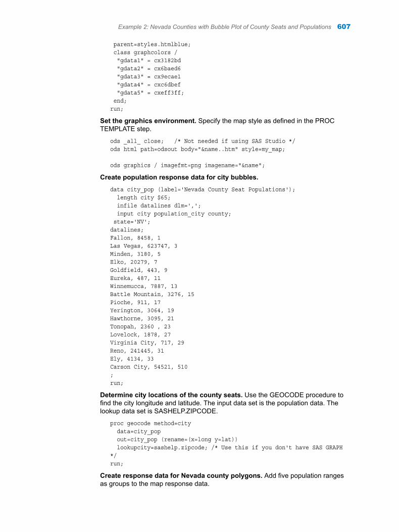
parent=styles.htmlblue; class graphcolors / "gdata1" = cx3182bd "gdata2" = cx6baed6 "gdata3" = cx9ecae1 "gdata4" = cxc6dbef "gdata5" = cxeff3ff; end;run;
Set the graphics environment. Specify the map style as defined in the PROC TEMPLATE step.
ods _all_ close; /* Not needed if using SAS Studio */ods html path=odsout body="&name..htm" style=my_map;
ods graphics / imagefmt=png imagename="&name";
Create population response data for city bubbles.
data city_pop (label='Nevada County Seat Populations'); length city $65; infile datalines dlm=','; input city population_city county; state='NV';datalines;Fallon, 8458, 1Las Vegas, 623747, 3Minden, 3180, 5Elko, 20279, 7Goldfield, 443, 9Eureka, 487, 11Winnemucca, 7887, 13Battle Mountain, 3276, 15Pioche, 911, 17Yerington, 3064, 19Hawthorne, 3095, 21Tonopah, 2360 , 23Lovelock, 1878, 27Virginia City, 717, 29Reno, 241445, 31Ely, 4134, 33Carson City, 54521, 510;run;
Determine city locations of the county seats. Use the GEOCODE procedure to find the city longitude and latitude. The input data set is the population data. The lookup data set is SASHELP.ZIPCODE.
proc geocode method=city data=city_pop out=city_pop (rename=(x=long y=lat)) lookupcity=sashelp.zipcode; /* Use this if you don't have SAS GRAPH */run;
Create response data for Nevada county polygons. Add five population ranges as groups to the map response data.
Example 2: Nevada Counties with Bubble Plot of County Seats and Populations 607

data county_pop (label='Nevada Counties');length county_name $55;infile datalines dlm=',';input county_name county population_county;statecode='NV';/* Add five population ranges as groups to map response data. */ if population_county > 100000 then group='Greater than 100,000'; else if population_county > 10000 then group='10,000 - 100,000'; else if population_county > 5000 then group='5,000 - 10,000'; else if population_county > 1000 then group='1,000 - 5,000'; else group='Less than 1,000';datalines;Churchill, 1, 24877Clark, 3, 2069681Douglas, 5, 47710Elko, 7, 52766Esmeralda, 9, 783Eureka, 11, 1987Humboldt, 13, 17019Lander, 15, 5775Lincoln, 17, 5036Lyon, 19, 52585Mineral, 21, 4772Nye, 23, 43946Pershing, 27, 6753Storey, 29, 3987Washoe, 31, 446903White Pine, 33, 10030Carson City, 510, 54521;run;
Sort the county population response data in descending order. This controls the order of the population groups in the legend.
proc sort data=county_pop; by descending population_county; run;
Retrieve county boundaries for the choropleth map.
data nevada; set mapsgfk.us_counties(where=(statecode='NV'));run;
Set the title of the map.
title 'Nevada County Seats and Populations';
Create the choropleth map and the legends. MAPDATA contains the state of Nevada's polygon coordinates. MAPRESPDATA contains the county population response data and PLOTDATA contains the BUBBLE city response data and location data.
proc sgmap mapdata=nevada /* Map polygon geometry */
608 Chapter 16 / SGMAP Procedure

maprespdata=county_pop /* Map polygon response data */ plotdata=city_pop /* Bubble response & location data */ ; choromap group / mapid=county id=county name='counties'; bubble x=long y=lat size=population_city / fillattrs=(color=yellow) name='cities' datalabel=city datalabelattrs=(color=black size=9 style=italic); keylegend 'counties' / title='County Population'; keylegend 'cities' / title='City Population';run;
quit;ods html close; /* Not needed if using SAS Studio */ods html; /* Not needed if using SAS Studio */
Example 3: Series Plot of Hurricane Katrina’s PathFeatures: PLOTDATA= argument referring to plot data
OPENSTREETMAP (OSM) statementSERIES statement options
LEGENDLABEL=LINEATTRS=
BUBBLE statement optionsDATALABEL=DATALABELPOS=DATALABELATTRS= with COLOR=, SIZE=, and STYLE= suboptionsLEGENDLABEL=
ODS destination statementDATA step with datetime format and informat, and datestringTITLE global statement
Data set: OpenStreetMap
ODS destination:
HTML
Sample library member:
SGMPBUSE
Notes: The SAS Sample Library is not available in SAS Studio.You can download the mapping samples in the SAS Sample Library in zipped format from the SAS/GRAPH Learning and Support page on support.sas.com. Click the link for SAS/GRAPH and Base SAS: Mapping Reference (Examples ZIP).The map data set or data sets supplied by SAS and used in this program might not be an available resource on your system.
This example overlays a bubble plot of wind speeds and a series plot of hurricane Katrina tracking locations onto an OpenStreetMap of the southeast United States. The bubble sizes are based on the wind speed. HTML output is displayed.
Example 3: Series Plot of Hurricane Katrina’s Path 609

Note: This example cannot be run without having SAS/GRAPH installed.
Output
Program%let name=sgmpbuse;filename odsout '.';
ods _all_ close; /* Not needed if using SAS Studio */ods html path=odsout body="&name..htm" style=htmlblue;
ods graphics / imagefmt=png imagename="&name";
data katrina;format datetime datetime18.;informat datetime datetime18.;infile datalines dlm=',';input datetime lat long wind;datestring=substr(put(datepart(datetime),date9.),1,5);datalines;23AUG2005:18:00:00,23.1,-75.1,30
610 Chapter 16 / SGMAP Procedure

24AUG2005:06:00:00,23.8,-76.2,3025AUG2005:06:00:00,26.1,-78.4,5026AUG2005:06:00:00,25.4,-81.3,6527AUG2005:06:00:00,24.4,-84,9528AUG2005:06:00:00,25.2,-86.7,12529AUG2005:06:00:00,28.2,-89.6,12530AUG2005:06:00:00,34.1,-88.6,4031AUG2005:06:00:00,40.1,-82.9,25;run;
title1 'Hurricane Katrina (2005)';
proc sgmap plotdata=katrina; openstreetmap;
series x=long y=lat / lineattrs=(color=red thickness=2) legendlabel='Storm Track'; bubble x=long y=lat size=wind / datalabel=datestring datalabelpos=left datalabelattrs=(color=red size=10) legendlabel='Relative Wind Speed';run;
quit;ods html close; /* Not needed if using SAS Studio */ods html; /* Not needed if using SAS Studio */
Program DescriptionPlot bubbles as hurricane wind speeds and plot series lines as hurricane tracking locations. Overlay plots on the southeast United States OpenStreetMap.
Set the graphics environment. Define the output filename and set the map output ODS destination to HTML.
%let name=sgmpbuse;filename odsout '.';
ods _all_ close; /* Not needed if using SAS Studio */ods html path=odsout body="&name..htm" style=htmlblue;
ods graphics / imagefmt=png imagename="&name";
Create hurricane location response data for the series lines and wind speed for the bubbles. The data includes the track locations at 6:00 am, as well as the first and last time record.
data katrina;format datetime datetime18.;informat datetime datetime18.;infile datalines dlm=',';input datetime lat long wind;datestring=substr(put(datepart(datetime),date9.),1,5);datalines;23AUG2005:18:00:00,23.1,-75.1,30
Example 3: Series Plot of Hurricane Katrina’s Path 611

24AUG2005:06:00:00,23.8,-76.2,3025AUG2005:06:00:00,26.1,-78.4,5026AUG2005:06:00:00,25.4,-81.3,6527AUG2005:06:00:00,24.4,-84,9528AUG2005:06:00:00,25.2,-86.7,12529AUG2005:06:00:00,28.2,-89.6,12530AUG2005:06:00:00,34.1,-88.6,4031AUG2005:06:00:00,40.1,-82.9,25;run;
Set the title for the graph. Use the global TITLE statement.
title1 'Hurricane Katrina (2005)';
Create the OpenStreetMap and plot overlays. Run the SGMAP procedure starting with the OpenStreetMap statement. Overlay the series plot of hurricane tracking locations in longitude and latitude coordinates. Assign a legend label for the series line depicting the hurricane’s track. Overlay the bubble plot of wind speeds. Use the BUBBLE statement options to specify the appearance of the bubble markers. Assign a legend label for the bubble markers with the BUBBLE statement’s LEGENDLABEL= option.
proc sgmap plotdata=katrina; openstreetmap;
series x=long y=lat / lineattrs=(color=red thickness=2) legendlabel='Storm Track'; bubble x=long y=lat size=wind / datalabel=datestring datalabelpos=left datalabelattrs=(color=red size=10) legendlabel='Relative Wind Speed';run;
quit;ods html close; /* Not needed if using SAS Studio */ods html; /* Not needed if using SAS Studio */
Example 4: Gradient Legend Showing 2010 U.S. PopulationFeatures: MAPDATA= argument for the map polygon data
PLOTDATA= argument referring to plot dataMAPRESPDATA= argument referring to response dataOPENSTREETMAP (OSM) statementESRIMAP statement (includes URL to service)TEXT statementCHOROMAP statement options
DENSITY=NAME= data descriptor referenced by GRADLEGEND statement
TEXT statement optionsTEXTATTRS= option with SIZE= suboption
612 Chapter 16 / SGMAP Procedure

GRADLEGEND statement optionsTITLE= for the gradient legendEXTRACTSCALE option reduces tick value width with the tick value scale factor
ODS destination statementDATA stepTITLE global statement
Data sets: MAPS.USCENTER (available without SAS/GRAPH)Esri Map service
ODS destination:
HTML
Sample library member:
SGMPGRAD
Notes: This example includes a network request. Note that these procedures do not authenticate any services that you specify, such as the map services and portal hosted by Esri. On a Windows operating system, check your proxy settings by entering the map service URL into a Windows Edge browser. This browser uses the same proxy settings as those set by the SAS installation system administrator. If the URL resolves, then you can use the URL in your SAS code without triggering a time-out. On a Linux operating system, if the SAS code to create an SGMAP times out, you can try the "curl" command with the map service URL. This might enable the SAS code to run to completion. Otherwise, check with your system administrator regarding the authentication setup for any Windows or Linux network proxy machine request that you might need to make.The SAS Sample Library is not available in SAS Studio.You can download the mapping samples in the SAS Sample Library in zipped format from the SAS/GRAPH Learning and Support page on support.sas.com. Click the link for SAS/GRAPH and Base SAS: Mapping Reference (Examples ZIP).The map data set or data sets supplied by SAS and used in this program might not be an available resource on your system.
This example overlays a choropleth map of population densities of the lower 48 states of the United States onto an Esri Map of the world. The state population variations are displayed by a gradient legend of ever darkening color as the population density increases.
Note: This example can be run without having SAS/GRAPH installed.
Example 4: Gradient Legend Showing 2010 U.S. Population 613

Output
Programods _all_ close; /* Not needed if using SAS Studio */ods html file="usPopgradlgnd.html";
data states; set maps.states; if state ^in(2,15,72); x = -x * 45/atan(1); y = y * 45/atan(1);run;
data plot_data; set maps.uscenter; if state ^in(2,15,72) and ocean^='Y'; long = -long; statename = fipstate(state);run;
title 'Population from 2010 US Census';
proc sgmap mapdata=states maprespdata=sashelp.us_data plotdata=plot_data;
614 Chapter 16 / SGMAP Procedure

esrimap url='https://services.arcgisonline.com/arcgis/rest/services/Canvas/World_Light_Gray_Base';
choromap population_2010 / mapid=state density=2 name='choro';
text x=long y=lat text=statename / textattrs=(size=6pt);
gradlegend 'choro' / title='2010 Population' extractscale;
run;
quit;
ods html close; /* Not needed if using SAS Studio */ods html; /* Not needed if using SAS Studio */
Program DescriptionPlot 2010 U.S. Census Bureau population densities of the lower 48 states of the United States onto an Esri map.
Define the output filename and set the map output ODS destination to HTML.
ods _all_ close; /* Not needed if using SAS Studio */ods html file="usPopgradlgnd.html";
The CHOROMAP statement plots the X (longitude) and Y (latitude) variables from the MAPS data set that contains unprojected latitude and longitude values. To match the projection types, convert the X and Y variables from radians to degrees.
data states; set maps.states; if state ^in(2,15,72); x = -x * 45/atan(1); y = y * 45/atan(1);run;
Create the plot data, used by the SGMAP procedure statement and the TEXT statement. Keep only the lower 48 U.S. states, collecting the state FIPS codes.
data plot_data; set maps.uscenter; if state ^in(2,15,72) and ocean^='Y'; long = -long; statename = fipstate(state);run;
Assign a title to the graph. Use the global TITLE statement.
title 'Population from 2010 US Census';
Create the graph. Run the SGMAP procedure, using as input the states map data set, the U.S. Census Bureau 2010 population response data, and the plot data set.
Example 4: Gradient Legend Showing 2010 U.S. Population 615
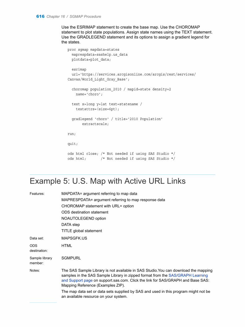
Use the ESRIMAP statement to create the base map. Use the CHOROMAP statement to plot state populations. Assign state names using the TEXT statement. Use the GRADLEGEND statement and its options to assign a gradient legend for the states.
proc sgmap mapdata=states maprespdata=sashelp.us_data plotdata=plot_data;
esrimap url='https://services.arcgisonline.com/arcgis/rest/services/Canvas/World_Light_Gray_Base';
choromap population_2010 / mapid=state density=2 name='choro';
text x=long y=lat text=statename / textattrs=(size=6pt);
gradlegend 'choro' / title='2010 Population' extractscale;
run;
quit;
ods html close; /* Not needed if using SAS Studio */ods html; /* Not needed if using SAS Studio */
Example 5: U.S. Map with Active URL LinksFeatures: MAPDATA= argument referring to map data
MAPRESPDATA= argument referring to map response dataCHOROMAP statement with URL= optionODS destination statementNOAUTOLEGEND optionDATA stepTITLE global statement
Data set: MAPSGFK.US
ODS destination:
HTML
Sample library member:
SGMPURL
Notes: The SAS Sample Library is not available in SAS Studio.You can download the mapping samples in the SAS Sample Library in zipped format from the SAS/GRAPH Learning and Support page on support.sas.com. Click the link for SAS/GRAPH and Base SAS: Mapping Reference (Examples ZIP).The map data set or data sets supplied by SAS and used in this program might not be an available resource on your system.
616 Chapter 16 / SGMAP Procedure

This example generates an HTML map of the United States. As your cursor hovers over a state, population data and the state abbreviation is revealed. The output map shown next reveals the state of Texas information. You can click to link to that or any state’s home website.
Note: This example cannot be run without having SAS/GRAPH installed.
Output
Programods _all_ close; /* Not needed if using SAS Studio */ods html path='.' body="sgmpurl.htm" style=htmlblue;ods graphics / imagefmt=png imagename="sgmpurl" imagemap tipmax=2500 width=500px height=375px;
title1 h=18pt "Click State to Link to State Home Page";
data my_data;
Example 5: U.S. Map with Active URL Links 617

set sashelp.us_data;length my_link $100;my_link='https://www.google.com/search?q=state+page+for+'||trim(left(statecode));run;
proc sgmap maprespdata=my_data mapdata=mapsgfk.us noautolegend;choromap population_2010 / mapid=statecode id=statecode url=my_link;run;
quit;ods html close; /* Not needed if using SAS Studio */ods html; /* Not needed if using SAS Studio */
Program DescriptionCreate a U.S. map with URL hot links to state websites.
Define the output filename and set the map output ODS destination to HTML.
ods _all_ close; /* Not needed if using SAS Studio */ods html path='.' body="sgmpurl.htm" style=htmlblue;ods graphics / imagefmt=png imagename="sgmpurl" imagemap tipmax=2500 width=500px height=375px;
Assign a title to the graph. Use the global TITLE statement.
title1 h=18pt "Click State to Link to State Home Page";
Create the response data set of URLs. Use a GOOGLE search to determine the website address for each state. Not every state uses the same URL address format.
data my_data; set sashelp.us_data;length my_link $100;my_link='https://www.google.com/search?q=state+page+for+'||trim(left(statecode));run;
Generate the choropleth U.S. map with hot links. Run the SGMAP procedure and define the map data set and the response data set. No automatic legend is specified. The CHOROMAP statement creates the choropleth map with 2010 population census data, the two–character state code, and the URL per state. As your cursor hovers over a state, the population and the two-character state code is revealed. When you click your cursor on a state, you link to the state’s home website.
proc sgmap maprespdata=my_data mapdata=mapsgfk.us noautolegend;choromap population_2010 / mapid=statecode id=statecode url=my_link;run;
618 Chapter 16 / SGMAP Procedure

quit;ods html close; /* Not needed if using SAS Studio */ods html; /* Not needed if using SAS Studio */
Example 5: U.S. Map with Active URL Links 619

620 Chapter 16 / SGMAP Procedure