
The OPTMODEL Procedure - SAS Support
176
SAS/OR ® 14.2 User’s Guide: Mathematical Programming The OPTMODEL Procedure
-
Upload
khangminh22 -
Category
Documents
-
view
0 -
download
0
Transcript of The OPTMODEL Procedure - SAS Support

SAS/OR® 14.2 User’s Guide:Mathematical ProgrammingThe OPTMODELProcedure

This document is an individual chapter from SAS/OR® 14.2 User’s Guide: Mathematical Programming.
The correct bibliographic citation for this manual is as follows: SAS Institute Inc. 2016. SAS/OR® 14.2 User’s Guide: MathematicalProgramming. Cary, NC: SAS Institute Inc.
SAS/OR® 14.2 User’s Guide: Mathematical Programming
Copyright © 2016, SAS Institute Inc., Cary, NC, USA
All Rights Reserved. Produced in the United States of America.
For a hard-copy book: No part of this publication may be reproduced, stored in a retrieval system, or transmitted, in any form or byany means, electronic, mechanical, photocopying, or otherwise, without the prior written permission of the publisher, SAS InstituteInc.
For a web download or e-book: Your use of this publication shall be governed by the terms established by the vendor at the timeyou acquire this publication.
The scanning, uploading, and distribution of this book via the Internet or any other means without the permission of the publisher isillegal and punishable by law. Please purchase only authorized electronic editions and do not participate in or encourage electronicpiracy of copyrighted materials. Your support of others’ rights is appreciated.
U.S. Government License Rights; Restricted Rights: The Software and its documentation is commercial computer softwaredeveloped at private expense and is provided with RESTRICTED RIGHTS to the United States Government. Use, duplication, ordisclosure of the Software by the United States Government is subject to the license terms of this Agreement pursuant to, asapplicable, FAR 12.212, DFAR 227.7202-1(a), DFAR 227.7202-3(a), and DFAR 227.7202-4, and, to the extent required under U.S.federal law, the minimum restricted rights as set out in FAR 52.227-19 (DEC 2007). If FAR 52.227-19 is applicable, this provisionserves as notice under clause (c) thereof and no other notice is required to be affixed to the Software or documentation. TheGovernment’s rights in Software and documentation shall be only those set forth in this Agreement.
SAS Institute Inc., SAS Campus Drive, Cary, NC 27513-2414
November 2016
SAS® and all other SAS Institute Inc. product or service names are registered trademarks or trademarks of SAS Institute Inc. in theUSA and other countries. ® indicates USA registration.
Other brand and product names are trademarks of their respective companies.
SAS software may be provided with certain third-party software, including but not limited to open-source software, which islicensed under its applicable third-party software license agreement. For license information about third-party software distributedwith SAS software, refer to http://support.sas.com/thirdpartylicenses.

Chapter 5
The OPTMODEL Procedure
ContentsOverview: OPTMODEL Procedure . . . . . . . . . . . . . . . . . . . . . . . . . . . . . . 26Getting Started: OPTMODEL Procedure . . . . . . . . . . . . . . . . . . . . . . . . . . . 27
An Unconstrained Optimization Example . . . . . . . . . . . . . . . . . . . . . . . . 28The Rosenbrock Problem . . . . . . . . . . . . . . . . . . . . . . . . . . . . . . . . 31A Transportation Problem . . . . . . . . . . . . . . . . . . . . . . . . . . . . . . . . 32
Syntax: OPTMODEL Procedure . . . . . . . . . . . . . . . . . . . . . . . . . . . . . . . . 34Functional Summary . . . . . . . . . . . . . . . . . . . . . . . . . . . . . . . . . . . 36PROC OPTMODEL Statement . . . . . . . . . . . . . . . . . . . . . . . . . . . . . 38Declaration Statements . . . . . . . . . . . . . . . . . . . . . . . . . . . . . . . . . . 42Programming Statements . . . . . . . . . . . . . . . . . . . . . . . . . . . . . . . . 51
Details: OPTMODEL Procedure . . . . . . . . . . . . . . . . . . . . . . . . . . . . . . . . 93Named Parameters . . . . . . . . . . . . . . . . . . . . . . . . . . . . . . . . . . . . 93Indexing . . . . . . . . . . . . . . . . . . . . . . . . . . . . . . . . . . . . . . . . . 94Types . . . . . . . . . . . . . . . . . . . . . . . . . . . . . . . . . . . . . . . . . . . 95Names . . . . . . . . . . . . . . . . . . . . . . . . . . . . . . . . . . . . . . . . . . 96Parameters . . . . . . . . . . . . . . . . . . . . . . . . . . . . . . . . . . . . . . . . 96Expressions . . . . . . . . . . . . . . . . . . . . . . . . . . . . . . . . . . . . . . . . 98Identifier Expressions . . . . . . . . . . . . . . . . . . . . . . . . . . . . . . . . . . 100Function Expressions . . . . . . . . . . . . . . . . . . . . . . . . . . . . . . . . . . 101Index Sets . . . . . . . . . . . . . . . . . . . . . . . . . . . . . . . . . . . . . . . . 102OPTMODEL Expression Extensions . . . . . . . . . . . . . . . . . . . . . . . . . . 103Conditions of Optimality . . . . . . . . . . . . . . . . . . . . . . . . . . . . . . . . . 112Data Set Input/Output . . . . . . . . . . . . . . . . . . . . . . . . . . . . . . . . . . 115Control Flow . . . . . . . . . . . . . . . . . . . . . . . . . . . . . . . . . . . . . . . 119Formatted Output . . . . . . . . . . . . . . . . . . . . . . . . . . . . . . . . . . . . 119ODS Table and Variable Names . . . . . . . . . . . . . . . . . . . . . . . . . . . . . 121Constraints . . . . . . . . . . . . . . . . . . . . . . . . . . . . . . . . . . . . . . . . 127Suffixes . . . . . . . . . . . . . . . . . . . . . . . . . . . . . . . . . . . . . . . . . . 131Integer Variable Suffixes . . . . . . . . . . . . . . . . . . . . . . . . . . . . . . . . . 135Dual Values . . . . . . . . . . . . . . . . . . . . . . . . . . . . . . . . . . . . . . . 136Reduced Costs . . . . . . . . . . . . . . . . . . . . . . . . . . . . . . . . . . . . . . 142Presolver . . . . . . . . . . . . . . . . . . . . . . . . . . . . . . . . . . . . . . . . . 143Model Update . . . . . . . . . . . . . . . . . . . . . . . . . . . . . . . . . . . . . . 143Multiple Subproblems . . . . . . . . . . . . . . . . . . . . . . . . . . . . . . . . . . 148Multiple Solutions . . . . . . . . . . . . . . . . . . . . . . . . . . . . . . . . . . . . 149Problem Symbols . . . . . . . . . . . . . . . . . . . . . . . . . . . . . . . . . . . . 150
26 F Chapter 5: The OPTMODEL Procedure
OPTMODEL Options . . . . . . . . . . . . . . . . . . . . . . . . . . . . . . . . . . 151Automatic Differentiation . . . . . . . . . . . . . . . . . . . . . . . . . . . . . . . . 152Conversions . . . . . . . . . . . . . . . . . . . . . . . . . . . . . . . . . . . . . . . 153FCMP Routines . . . . . . . . . . . . . . . . . . . . . . . . . . . . . . . . . . . . . 154More on Index Sets . . . . . . . . . . . . . . . . . . . . . . . . . . . . . . . . . . . 157Threaded and Distributed Processing . . . . . . . . . . . . . . . . . . . . . . . . . . 158Macro Variable _OROPTMODEL_ . . . . . . . . . . . . . . . . . . . . . . . . . . . 159Rewriting PROC NLP Models for PROC OPTMODEL . . . . . . . . . . . . . . . . 161
Examples: OPTMODEL Procedure . . . . . . . . . . . . . . . . . . . . . . . . . . . . . . 164Example 5.1: Matrix Square Root . . . . . . . . . . . . . . . . . . . . . . . . . . . . 164Example 5.2: Reading From and Creating a Data Set . . . . . . . . . . . . . . . . . . 165Example 5.3: Model Construction . . . . . . . . . . . . . . . . . . . . . . . . . . . . 167Example 5.4: Set Manipulation . . . . . . . . . . . . . . . . . . . . . . . . . . . . . 171Example 5.5: Multiple Subproblems . . . . . . . . . . . . . . . . . . . . . . . . . . . 172Example 5.6: Traveling Salesman Problem . . . . . . . . . . . . . . . . . . . . . . . 176Example 5.7: Sparse Modeling . . . . . . . . . . . . . . . . . . . . . . . . . . . . . 180Example 5.8: Chemical Equilibrium . . . . . . . . . . . . . . . . . . . . . . . . . . . 186
References . . . . . . . . . . . . . . . . . . . . . . . . . . . . . . . . . . . . . . . . . . . 190
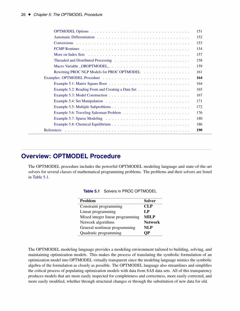
Overview: OPTMODEL ProcedureThe OPTMODEL procedure includes the powerful OPTMODEL modeling language and state-of-the-artsolvers for several classes of mathematical programming problems. The problems and their solvers are listedin Table 5.1.
Table 5.1 Solvers in PROC OPTMODEL
Problem SolverConstraint programming CLPLinear programming LPMixed integer linear programming MILPNetwork algorithms NetworkGeneral nonlinear programming NLPQuadratic programming QP
The OPTMODEL modeling language provides a modeling environment tailored to building, solving, andmaintaining optimization models. This makes the process of translating the symbolic formulation of anoptimization model into OPTMODEL virtually transparent since the modeling language mimics the symbolicalgebra of the formulation as closely as possible. The OPTMODEL language also streamlines and simplifiesthe critical process of populating optimization models with data from SAS data sets. All of this transparencyproduces models that are more easily inspected for completeness and correctness, more easily corrected, andmore easily modified, whether through structural changes or through the substitution of new data for old.

Getting Started: OPTMODEL Procedure F 27
In addition to invoking optimization solvers directly with PROC OPTMODEL as already mentioned, you canuse the OPTMODEL language purely as a modeling facility. You can save optimization models built with theOPTMODEL language in SAS data sets that can be submitted to other SAS/OR optimization procedures. Ingeneral, the OPTMODEL language serves as a common point of access for many of the SAS/OR optimizationcapabilities, whether providing both modeling and solver access or acting as a modeling interface for otheroptimization procedures.
For details and examples of the problems addressed and corresponding solvers, please see the dedicated chap-ters in this book. This chapter aims to give you a comprehensive understanding of the OPTMODEL procedureby discussing the framework provided by the OPTMODEL modeling language. For additional examplesthat demonstrate the features of the OPTMODEL procedure, see SAS/OR User’s Guide: MathematicalProgramming Examples.
The OPTMODEL modeling language features automatic differentiation, advanced flow control, optimization-oriented syntax (parameters, variables, arrays, constraints, objective functions), dynamic model generation,model-data separation, and transparent access to SAS data sets.
Getting Started: OPTMODEL ProcedureOptimization or mathematical programming is a search for a maximum or minimum of an objective function(also called a cost function), where search variables are restricted to particular constraints. Constraints aresaid to define a feasible region (see Figure 5.1).
Figure 5.1 Examples of Feasible Regions
A more rigorous general formulation of such problems is as follows.
Let
f W S ! R
be a real-valued function. Find x� such that
� x� 2 S

28 F Chapter 5: The OPTMODEL Procedure
� f .x�/ � f .x/; 8x 2 S
Note that the formulation is for the minimum of f and that the maximum of f is simply the negation of theminimum of �f .
Here, function f is the objective function, and the variable in the objective function is called the optimizationvariable (or decision variable). S is the feasible region. Typically S is a subset of the Euclidean space Rn
specified by the set of constraints, which are often a set of equalities (=) or inequalities (�;�) that everyelement in S is required to satisfy simultaneously. For the special case where S D Rn, the problem is anunconstrained optimization. An element x of S is called a feasible solution to the optimization problem, andthe value f .x/ is called the objective value. A feasible solution x� that minimizes the objective function iscalled an optimal solution to the optimization problem, and the corresponding objective value is called theoptimal value.
In mathematics, special notation is used to denote an optimization problem. Generally, you can write anoptimization problem as follows:
minimize f .x/
subject to x 2 S
Normally, an empty body of constraint (the part after “subject to”) implies that the optimization is un-constrained (that is, the feasible region is the whole space Rn). The optimal solution (x�) is denotedas
x� D argminx2S
f .x/
The optimal value (f .x�/) is denoted as
f .x�/ D minx2S
f .x/
Optimization problems can be classified by the forms (linear, quadratic, nonlinear, and so on) of the functionsin the objective and constraints. For example, a problem is said to be linearly constrained if the functionsin the constraints are linear. A linear programming problem is a linearly constrained problem with a linearobjective function. A nonlinear programming problem occurs where some function in the objective orconstraints is nonlinear, and so on.
An Unconstrained Optimization ExampleAn unconstrained optimization problem formulation is simply
minimize f .x/
For example, suppose you wanted to find the minimum value of this polynomial:
z.x; y/ D x2 � x � 2y � xy C y2

An Unconstrained Optimization Example F 29
You can compactly specify and solve the optimization problem by using the OPTMODEL modeling language.Here is the program:
/* invoke procedure */proc optmodel;
var x, y; /* declare variables */
/* objective function */min z=x**2 - x - 2*y - x*y + y**2;
/* now run the solver */solve;
print x y;quit;
This program produces the output in Figure 5.2.
Figure 5.2 Optimizing a Simple Polynomial
The OPTMODEL ProcedureThe OPTMODEL Procedure
Problem Summary
Objective Sense Minimization
Objective Function z
Objective Type Quadratic
Number of Variables 2
Bounded Above 0
Bounded Below 0
Bounded Below and Above 0
Free 2
Fixed 0
Number of Constraints 0
Constraint Coefficients 0
Performance Information
Execution Mode Single-Machine
Number of Threads 4

30 F Chapter 5: The OPTMODEL Procedure
Figure 5.2 continued
Solution Summary
Solver QP
Algorithm Interior Point
Objective Function z
Solution Status Optimal
Objective Value -2.333333333
Primal Infeasibility 0
Dual Infeasibility 6.861556E-17
Bound Infeasibility 0
Duality Gap 0
Complementarity 0
Iterations 0
Presolve Time 0.00
Solution Time 0.02
x y
1.3333 1.6667
In PROC OPTMODEL you specify the mathematical formulas that describe the behavior of the optimizationproblem that you want to solve. In the preceding example there were two independent variables in thepolynomial, x and y. These are the optimization variables of the problem. In PROC OPTMODEL you declareoptimization variables with the VAR statement. The formula that defines the quantity that you are seekingto optimize is called the objective function, or objective. The solver varies the values of the optimizationvariables when searching for an optimal value for the objective.
In the preceding example the objective function is named z, declared with the MIN statement. The keywordMIN is an abbreviation for MINIMIZE. The expression that follows the equal sign (=) in the MIN statementdefines the function to be minimized in terms of the optimization variables.
The VAR and MIN statements are just two of the many available PROC OPTMODEL declaration andprogramming statements. PROC OPTMODEL processes all such statements interactively, meaning that eachstatement is processed as soon as it is complete.
After PROC OPTMODEL has completed processing of declaration and programming statements, it processesthe SOLVE statement, which submits the problem to a solver and prints a summary of the results. The PRINTstatement displays the optimal values of the optimization variables x and y found by the solver.
It is worth noting that PROC OPTMODEL does not use a RUN statement but instead operates on aninteractive basis throughout. You can continue to interact with PROC OPTMODEL even after invoking asolver. For example, you could modify the problem and issue another SOLVE statement (see the section“Model Update” on page 143).

The Rosenbrock Problem F 31
The Rosenbrock ProblemYou can use parameters to produce a clear formulation of a problem. Consider the Rosenbrock problem,
minimize f .x1; x2/ D ˛ .x2 � x21/2C .1 � x1/
2
where ˛ D 100 is a parameter (constant), x1 and x2 are optimization variables (whose values are to bedetermined), and f .x1; x2/ is an objective function.
Here is a PROC OPTMODEL program that solves the Rosenbrock problem:
proc optmodel;number alpha = 100; /* declare parameter */var x {1..2}; /* declare variables *//* objective function */min f = alpha*(x[2] - x[1]**2)**2 +
(1 - x[1])**2;/* now run the solver */solve;
print x;quit;
The PROC OPTMODEL output is shown in Figure 5.3.
Figure 5.3 Rosenbrock Function Results
The OPTMODEL ProcedureThe OPTMODEL Procedure
Problem Summary
Objective Sense Minimization
Objective Function f
Objective Type Nonlinear
Number of Variables 2
Bounded Above 0
Bounded Below 0
Bounded Below and Above 0
Free 2
Fixed 0
Number of Constraints 0
Performance Information
Execution Mode Single-Machine
Number of Threads 4

32 F Chapter 5: The OPTMODEL Procedure
Figure 5.3 continued
Solution Summary
Solver NLP
Algorithm Interior Point
Objective Function f
Solution Status Optimal
Objective Value 8.204873E-23
Optimality Error 9.704881E-11
Infeasibility 0
Iterations 14
Presolve Time 0.00
Solution Time 0.01
[1] x
1 1
2 1
A Transportation ProblemYou can easily translate the symbolic formulation of a problem into the OPTMODEL procedure. Considerthe transportation problem, which is mathematically modeled as the following linear programming problem:
minimizeX
i2O;j2D
cijxij
subject toXj2D
xij D ai ; 8i 2 O .SUPPLY/Xi2O
xij D bj ; 8j 2 D .DEMAND/
xij � 0; 8.i; j / 2 O �D
where O is the set of origins, D is the set of destinations, cij is the cost to transport one unit from i to j, ai isthe supply of origin i, bj is the demand of destination j, and xij is the decision variable for the amount ofshipment from i to j.
Here is a very simple example. The cities in the set O of origins are Detroit and Pittsburgh. The cities in theset D of destinations are Boston and New York. The cost matrix, supply, and demand are shown in Table 5.2.
Table 5.2 A Transportation Problem
Boston New York SupplyDetroit 30 20 200
Pittsburgh 40 10 100Demand 150 150

A Transportation Problem F 33
The problem is compactly and clearly formulated and solved by using the OPTMODEL procedure with thefollowing statements:
proc optmodel;/* specify parameters */set O={'Detroit','Pittsburgh'};set D={'Boston','New York'};number c{O,D}=[30 20
40 10];number a{O}=[200 100];number b{D}=[150 150];/* model description */var x{O,D} >= 0;min total_cost = sum{i in O, j in D}c[i,j]*x[i,j];constraint supply{i in O}: sum{j in D}x[i,j]=a[i];constraint demand{j in D}: sum{i in O}x[i,j]=b[j];/* solve and output */solve;print x;
The output is shown in Figure 5.4.
Figure 5.4 Solution to the Transportation Problem
The OPTMODEL ProcedureThe OPTMODEL Procedure
Problem Summary
Objective Sense Minimization
Objective Function total_cost
Objective Type Linear
Number of Variables 4
Bounded Above 0
Bounded Below 4
Bounded Below and Above 0
Free 0
Fixed 0
Number of Constraints 4
Linear LE (<=) 0
Linear EQ (=) 4
Linear GE (>=) 0
Linear Range 0
Constraint Coefficients 8
Performance Information
Execution Mode Single-Machine
Number of Threads 1

34 F Chapter 5: The OPTMODEL Procedure
Figure 5.4 continued
Solution Summary
Solver LP
Algorithm Dual Simplex
Objective Function total_cost
Solution Status Optimal
Objective Value 6500
Primal Infeasibility 0
Dual Infeasibility 0
Bound Infeasibility 0
Iterations 0
Presolve Time 0.00
Solution Time 0.00
x
BostonNewYork
Detroit 150 50
Pittsburgh 0 100
Syntax: OPTMODEL ProcedurePROC OPTMODEL statements are divided into three categories: the PROC statement, the declarationstatements, and the programming statements. The PROC statement invokes the procedure and sets initialoption values. The declaration statements declare optimization model components. The programmingstatements read and write data, invoke the solver, and print results. In the following text, the statements arelisted in the order in which they are grouped, with declaration statements first.
NOTE: Solver specific options are described in the individual chapters that correspond to the solvers.

Syntax: OPTMODEL Procedure F 35
PROC OPTMODEL options ;
Declaration Statements:CONSTRAINT constraints ;IMPVAR optimization expression declarations ;MAX objective ;MIN objective ;NUMBER parameter declarations ;PROBLEM problem declaration ;SET Œ < types > � parameter declarations ;STRING parameter declarations ;VAR variable declarations ;
Programming Statements:Assignment parameter = expression ;CALL name Œ ( expressions ) � ;CLOSEFILE files ;COFOR { index-set } statement ;CONTINUE ;CREATE DATA SAS-data-set FROM columns ;DO ; statements ; END ;DO variable = specifications ; statements ; END ;DO UNTIL ( logic ) ; statements ; END ;DO WHILE ( logic ) ; statements ; END ;DROP constraint ;EXPAND name Œ / options � ;FILE file ;FIX variable Œ = expression � ;FOR { index-set } statement ;IF logic THEN statement ; Œ ELSE statement � ;LEAVE ;Null ;PERFORMANCE options ;PRINT print items ;PROFILE Œ mode � options ;PUT put items ;QUIT ;READ DATA SAS-data-set INTO columns ;RESET OPTIONS options ;RESTORE constraint ;SAVE MPS SAS-data-set Œ OBJECTIVE name � Œ NOOBJECTIVE � ;SAVE QPS SAS-data-set Œ OBJECTIVE name � Œ NOOBJECTIVE � ;SOLVE Œ WITH solver � Œ OBJECTIVE name � Œ NOOBJECTIVE � Œ RELAXINT � Œ / options � ;STOP ;SUBMIT arguments Œ / options � ;UNFIX variable Œ = expression � ;USE PROBLEM problem ;

36 F Chapter 5: The OPTMODEL Procedure
Functional SummaryThe statements and options available with PROC OPTMODEL are summarized by purpose in Table 5.3.
Table 5.3 Functional Summary
Description Statement Option
Declaration Statements:Declares a constraint CONSTRAINTDeclares optimization expressions IMPVARDeclares a maximization objective MAXDeclares a minimization objective MINDeclares a number type parameter NUMBERDeclares a problem PROBLEMDeclares a set type parameter SETDeclares a string type parameter STRINGDeclares optimization variables VAR
Programming Statements:Assigns a value to a variable or parameter =Invokes a library subroutine CALLCloses the opened file CLOSEFILEExecutes the statement repeatedly with support forconcurrent solver invocations
COFOR
Terminates one iteration of a loop statement CONTINUECreates a new SAS data set and copies data intoit from PROC OPTMODEL parameters and vari-ables
CREATE DATA
Groups a sequence of statements together as a sin-gle statement
DO
Executes statements repeatedly DO (iterative)Executes statements repeatedly until some condi-tion is satisfied
DO UNTIL
Executes statements repeatedly as long as somecondition is satisfied
DO WHILE
Ignores the specified constraint DROPPrints the specified constraint, variable, or objec-tive declaration expressions after expanding aggre-gation operators, and so on
EXPAND
Selects a file for the PUT statement FILETreats a variable as fixed in value FIXExecutes the statement repeatedly FORExecutes the statement conditionally IFTerminates the execution of the entire loop body LEAVENull statement ;Controls parallel execution PERFORMANCE

Functional Summary F 37
Description Statement Option
Outputs string and numeric data PRINTProvides timing and execution count informationfor statements and declarations
PROFILE
Writes text data to the current output file PUTTerminates the PROC OPTMODEL session QUITReads data from a SAS data set into PROC OPT-MODEL parameters and variables
READ DATA
Sets PROC OPTMODEL option values or restoresthem to their defaults
RESET OPTIONS
Adds a constraint that was previously droppedback into the model
RESTORE
Saves the structure and coefficients for a linearprogramming model into a SAS data set
SAVE MPS
Saves the structure and coefficients for a quadraticprogramming model into a SAS data set
SAVE QPS
Invokes a PROC OPTMODEL solver SOLVEHalts the execution of all statements that contain it STOPSubmits SAS code for execution SUBMITReverses the effect of FIX statement UNFIXSelects the current problem USE PROBLEM
PROC OPTMODEL Options:Specifies the accuracy for nonlinear constraints PROC OPTMODEL CDIGITS=Specifies the maximum number of error messagesdisplayed
PROC OPTMODEL ERRORLIMIT=
Specifies the method used to approximate numericderivatives
PROC OPTMODEL FD=
Specifies the accuracy for the objective function PROC OPTMODEL FDIGITS=Forces finite differences to be used for nonlinearequations
PROC OPTMODEL FORCEFD=
Enables the OPTMODEL presolver for the CLP,LP, MILP, and QP solvers
PROC OPTMODEL FORCEPRESOLVE=
Passes initial values for variables to the solver PROC OPTMODEL INITVAR/NOINITVARSpecifies the tolerance for rounding the bounds oninteger and binary variables
PROC OPTMODEL INTFUZZ=
Specifies the maximum length for MPS row andcolumn labels
PROC OPTMODEL MAXLABLEN=
Checks missing values PROC OPTMODEL MISSCHECK/NOMISSCHECKSpecifies the maximum number of non-error mes-sages displayed
PROC OPTMODEL MSGLIMIT=
Specifies the number of digits to display PROC OPTMODEL PDIGITS=Adjusts how two-dimensional array is displayed PROC OPTMODEL PMATRIX=Specifies the type of presolve performed by thePROC OPTMODEL presolver
PROC OPTMODEL PRESOLVER=

38 F Chapter 5: The OPTMODEL Procedure
Description Statement Option
Specifies the tolerance, enabling the PROC OPT-MODEL presolver to remove slightly infeasibleconstraints
PROC OPTMODEL PRESTOL=
Enables or disables printing summary PROC OPTMODEL PRINTLEVEL=Specifies the width to display numeric columns PROC OPTMODEL PWIDTH=Specifies the smallest difference that is permittedby the PROC OPTMODEL presolver between theupper and lower bounds of an unfixed variable
PROC OPTMODEL VARFUZZ=
PROC OPTMODEL StatementPROC OPTMODEL Œ options � ;
The PROC OPTMODEL statement invokes the OPTMODEL procedure. You can specify options to controlhow the optimization model is processed and how results are displayed. You can specify the followingoptions (these options can also be specified in the RESET OPTIONS statement).
CDIGITS=numberspecifies the expected number of decimal digits of accuracy for nonlinear constraints. The value canbe fractional. PROC OPTMODEL uses this option to choose a step length when numeric derivativeapproximations are required to evaluate the Jacobian of nonlinear constraints. The default valuedepends on your operating environment. It is assumed that constraint values are accurate to the limitsof machine precision.
See the section “Automatic Differentiation” on page 152 for more information about numeric derivativeapproximations.
ERRORLIMIT=number | NONEspecifies the maximum number of error messages that can be displayed during SOLVE statementprocessing. Specifying a value of number in the range 1 to 231 � 1 sets a specific limit. SpecifyingERRORLIMIT=NONE removes any existing limit. The default value is 10.
NOTE: Some errors abort processing immediately.
FD=FORWARD | CENTRALselects the method used to approximate numeric derivatives when analytic derivatives are unavailable.Most solvers require the derivatives of the objective and constraints. You can specify the followingvalues:
FORWARD uses forward differences.
CENTRAL uses central differences.
By default, FD=FORWARD. For more information about numeric derivative approximations, see thesection “Automatic Differentiation” on page 152.

PROC OPTMODEL Statement F 39
FDIGITS=numberspecifies the expected number of decimal digits of accuracy for the objective function. The value canbe fractional. PROC OPTMODEL uses the value to choose a step length when numeric derivativesare required. The default value depends on your operating environment. It is assumed that objectivefunction values are accurate to the limits of machine precision.
For more information about numeric derivative approximations, see the section “Automatic Differenti-ation” on page 152.
FORCEFD=NONE | OBJ | CON | ALLforces PROC OPTMODEL to use finite differences instead of analytic derivatives for the specified setof nonlinear expressions. This option can be useful with FCMP functions to provide more control overderivative computation. You can specify the following values:
ALL restricts all derivative computations to use finite differences.
CON restricts derivative computations for the nonlinear constraint expressions and anyIMPVAR expressions they reference to use finite differences.
NONE requests analytic derivatives where they are available.
OBJ restricts derivative computations for the objective and any IMPVAR expressions itreferences to use finite differences.
By default, FORCEFD=NONE.
FORCEPRESOLVE=number | stringspecifies whether PROC OPTMODEL can use the OPTMODEL presolver with the CLP, LP, MILP,and QP solvers. By default, the OPTMODEL presolver is disabled when PROC OPTMODEL solveslinear problems or problems with predicates, or when the CLP, LP, MILP, or QP solver is specified inthe SOLVE statement. Table 5.4 shows the valid values for this option.
Table 5.4 Values for the FORCEPRESOLVE= Option
number string Description0 OFF Restores the default behavior.1 ON Enables PROC OPTMODEL to use the OPT-
MODEL presolver when the CLP, LP, MILP, orQP solver is specified in the SOLVE statement.
By default, FORCEPRESOLVE=0.
INITVAR | NOINITVARselects whether or not to pass initial values for variables to the solver when the SOLVE statement isexecuted. INITVAR enables the current variable values to be passed. NOINITVAR causes the solverto be invoked without any specific initial values for variables. The INITVAR option is the default.
The CLP, LP, and QP solvers always ignore initial values. The NLP solvers attempt to use specifiedinitial values. The MILP solver uses initial values only if the PRIMALIN option is specified.

40 F Chapter 5: The OPTMODEL Procedure
INTFUZZ=numberspecifies the tolerance for rounding the bounds on integer and binary variables to integer values.Bounds that differ from an integer by at most number are rounded to that integer. Otherwise, lowerbounds are rounded up to the next greater integer and upper bounds are rounded down to the nextlesser integer. The value of number can range between 0 and 0.5. The default value is 0.00001.
MAXLABLEN=numberspecifies the maximum length for MPS row and column labels. The allowed range is 8 to 256. Thisoption can also be used to control the length of row and column names displayed by solvers, such asthose found in the LP solver iteration log. See also the description of the .label suffix in the section“Suffixes” on page 131. By default, MAXLABLEN=32.
MISSCHECK | NOMISSCHECKenables detailed checking of missing values in expressions. MISSCHECK requests that PROCOPTMODEL produce a message each time it evaluates an arithmetic operation or function that hasmissing value operands (except when the operation or function specifically supports missing values).The MISSCHECK option can increase processing time. NOMISSCHECK turns off this detailedreporting. NOMISSCHECK is the default.
MSGLIMIT=number | NONEspecifies the maximum number of messages about certain issues that can be displayed during processingof a single top-level statement, such as a SOLVE or FOR statement. Specifying a value of number inthe range 0 to 231 � 1 sets a specific limit. Specifying MSGLIMIT=NONE removes any existing limit.The default value is 25.
The limit is applied to notes and warnings for the following issues:
� arithmetic evaluation issues, such as division by zero
� function evaluation issues, such as invalid arguments
� problem generation and PROC OPTMODEL presolver issues
� duplicate members in set constructor and literal expressions
� string concatenation results truncated to the maximum string length
� duplicate READ DATA keys
� truncated data set column labels for the CREATE DATA statement
� misspelled keywords for an option value specified using a string expression
� unrecognized file specifications in the CLOSEFILE statement
NOTE: Because of complications of concurrent execution, PROC OPTMODEL might display more orfewer messages than the limit when you use a COFOR statement.
PDIGITS=numberrequests that the PRINT statement display number significant digits for numeric columns for which noformat is specified. The value can range from 1 to 9. By default, PDIGITS=5.
PMATRIX=numberadjusts the density evaluation of a two-dimensional array to affect how it is displayed. The valuenumber scales the total number of nonempty array elements and is used by the PRINT statementto evaluate whether a two-dimensional array is “sparse” or “dense.” Tables that contain a single

PROC OPTMODEL Statement F 41
two-dimensional array are printed in list form if they are sparse and in matrix form if they are dense.Any nonnegative value can be assigned to number . Specifying a value for the PMATRIX= option thatis less than 1 causes the list form to be used in more cases, whereas specifying a value greater than 1causes the matrix form to be used in more cases. If the value is 0, then the list form is always used. Formore information, see the section “PRINT Statement” on page 74. By default, PMATRIX=1.
PRESOLVER=number | stringspecifies the type of presolve that the OPTMODEL presolver performs. Table 5.5 shows the validvalues of this option.
Table 5.5 Values for the PRESOLVER= Option
number string Description–1 AUTOMATIC Applies presolver using default setting.0 NONE Disables presolver.1 BASIC Performs minimal processing, only substituting
fixed variables and removing empty feasible con-straints.
2 MODERATE Applies a higher level of presolve processing.3 AGGRESSIVE Applies the highest level of presolve processing.
The OPTMODEL presolver tightens variable bounds and eliminates redundant constraints. In general,this tightening improves the performance of any solver. Higher levels of presolve processing allowmore tightening and substitution passes, but might take more time to execute. The AUTOMATICoption is intermediate between the MODERATE and AGGRESSIVE levels.
NOTE: The OPTMODEL presolver is normally bypassed when PROC OPTMODEL uses the CLP,LP, QP, MILP, or network solver and when the SAVE MPS and SAVE QPS statements execute. TheFORCEPRESOLVE= option enables the OPTMODEL presolver to be used with the CLP, LP, QP, andMILP solvers. PROC OPTMODEL always bypasses the OPTMODEL presolver when you specifycertain solver options. For more information, see the chapter for the relevant solver in this book.
PRESTOL=numberprovides a tolerance so that slightly infeasible constraints can be eliminated by the OPTMODELpresolver. If the magnitude of the infeasibility is no greater than num.jXj C 1/, where X is the value ofthe original bound, then the empty constraint is removed from the presolved problem. OPTMODEL’spresolver does not print messages about infeasible constraints and variable bounds when the infeasibilityis within the PRESTOL tolerance. The value of PRESTOL can range between 0 and 0.1; the defaultvalue is 1E–12.
PRINTLEVEL=numbercontrols the level of listing output during a SOLVE or COFOR command. The Output Delivery System(ODS) tables printed at each level are listed in Table 5.6. Some solvers can produce additional tables;see the individual solver chapters for more information.
Table 5.6 Values for the PRINTLEVEL= Option
number Description0 Disables all tables.

42 F Chapter 5: The OPTMODEL Procedure
number Description1 Prints COFOR Performance Information, Problem Summary, Performance
Information, and Solution Summary.2 Prints COFOR Performance Information, Problem Summary, Performance
Information, Solution Summary, Methods of Derivative Computation (forNLP solvers), Solver Options, Optimization Statistics, and solver-specificODS tables.
For more information about the ODS tables produced by PROC OPTMODEL, see the section “ODSTable and Variable Names” on page 121.
PWIDTH=numbersets the width used by the PRINT statement to display numeric columns when no format is specified.The smallest value number can take is the value of the PDIGITS= option plus 7; the largest valuenumber can take is 16. The default value is equal to the value of the PDIGITS= option plus 7.
VARFUZZ=numberspecifies the smallest difference that is permitted by the OPTMODEL presolver between the upper andlower bounds of an unfixed variable. If the difference is smaller than number , then the variable isfixedto the average of the upper and lower bounds before it is presented to the solver. Any nonnegativevalue can be assigned to number ; the default value is 0.
Declaration StatementsThe declaration statements define the parameters, variables, constraints, and objectives that describe a PROCOPTMODEL optimization model. Declarations in the PROC OPTMODEL input are saved for later use.Unlike programming statements, declarations cannot be nested in other statements. Declaration statementsare terminated by a semicolon.
Many declaration attributes, such as variable bounds, are defined using expressions. Expressions in declara-tions are handled symbolically and are resolved as needed. In particular, expressions are generally reevaluatedwhen one of the parameter values they use has been changed.
CONSTRAINT Declaration
CONSTRAINT constraint Œ , . . . constraint � ;
CON constraint Œ , . . . constraint � ;
The constraint declaration defines one or more constraints on expressions in terms of the optimizationvariables. You can specify multiple constraint declaration statements.
Constraints can have an upper bound, a lower bound, or both bounds. The allowed forms are as follows:
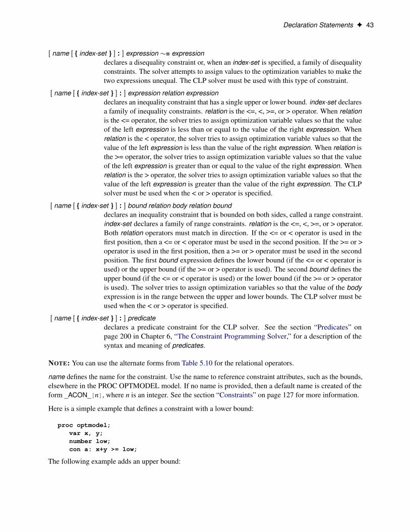
Œ name Œ { index-set } � : � expression = expressiondeclares an equality constraint or, when an index-set is specified, a family of equalityconstraints. The solver attempts to assign values to the optimization variables to make thetwo expressions equal.
Declaration Statements F 43
Œ name Œ { index-set } � : � expression �= expressiondeclares a disequality constraint or, when an index-set is specified, a family of disequalityconstraints. The solver attempts to assign values to the optimization variables to make thetwo expressions unequal. The CLP solver must be used with this type of constraint.
Œ name Œ { index-set } � : � expression relation expressiondeclares an inequality constraint that has a single upper or lower bound. index-set declaresa family of inequality constraints. relation is the <=, <, >=, or > operator. When relationis the <= operator, the solver tries to assign optimization variable values so that the valueof the left expression is less than or equal to the value of the right expression. Whenrelation is the < operator, the solver tries to assign optimization variable values so that thevalue of the left expression is less than the value of the right expression. When relation isthe >= operator, the solver tries to assign optimization variable values so that the valueof the left expression is greater than or equal to the value of the right expression. Whenrelation is the > operator, the solver tries to assign optimization variable values so that thevalue of the left expression is greater than the value of the right expression. The CLPsolver must be used when the < or > operator is specified.
Œ name Œ { index-set } � : � bound relation body relation bounddeclares an inequality constraint that is bounded on both sides, called a range constraint.index-set declares a family of range constraints. relation is the <=, <, >=, or > operator.Both relation operators must match in direction. If the <= or < operator is used in thefirst position, then a <= or < operator must be used in the second position. If the >= or >operator is used in the first position, then a >= or > operator must be used in the secondposition. The first bound expression defines the lower bound (if the <= or < operator isused) or the upper bound (if the >= or > operator is used). The second bound defines theupper bound (if the <= or < operator is used) or the lower bound (if the >= or > operatoris used). The solver tries to assign optimization variables so that the value of the bodyexpression is in the range between the upper and lower bounds. The CLP solver must beused when the < or > operator is specified.
Œ name Œ { index-set } � : � predicatedeclares a predicate constraint for the CLP solver. See the section “Predicates” onpage 200 in Chapter 6, “The Constraint Programming Solver,” for a description of thesyntax and meaning of predicates.
NOTE: You can use the alternate forms from Table 5.10 for the relational operators.
name defines the name for the constraint. Use the name to reference constraint attributes, such as the bounds,elsewhere in the PROC OPTMODEL model. If no name is provided, then a default name is created of theform _ACON_[n], where n is an integer. See the section “Constraints” on page 127 for more information.
Here is a simple example that defines a constraint with a lower bound:
proc optmodel;var x, y;number low;con a: x+y >= low;
The following example adds an upper bound:

44 F Chapter 5: The OPTMODEL Procedure
var x, y;number low;con a: low <= x+y <= low+10;
Indexed families of constraints can be defined by specifying an index-set after the name. Any dummyparameters that are declared in the index-set can be referenced in the expressions that define the constraint.A particular member of an indexed family can be specified by using an identifier-expression with a bracketedindex list, in the same fashion as array parameters and variables. For example, the following statementscreate an indexed family of constraints named incr:
proc optmodel;number n;var x{1..n}/* require nondecreasing x values */con incr{i in 1..n-1}: x[i+1] >= x[i];
The CON statement in the example creates constraints incr[1] through incr[n–1].
Constraint expressions cannot be defined using functions that return different values each time they are called.See the section “Indexing” on page 94 for details.
IMPVAR Declaration
IMPVAR impvar-decl Œ , . . . impvar-decl � ;
The IMPVAR declaration specifies one or more names that refer to optimization expressions in the model.The declared name is called an implicit variable. An implicit variable is useful for structuring models so thatcomplex expressions do not need to be repeated each time they are used. The value of an implicit variableneeds to be computed only once instead of at each place where the original expression is used, which helpsreduce computational overhead. Implicit variables are evaluated without intervention from the solver.
Multiple IMPVAR declarations are allowed. The names of implicit variables must be distinct from othermodel declarations, such as variables and constraints. Implicit variables can be used in model expressions inthe same places where ordinary variables are allowed.
This is the syntax for an impvar-decl:
name Œ { index-set } � = expression
Each impvar-decl declares a name for an implicit variable. The name can be followed by an index-setspecification to declare a family of implicit variables. The expression that the name refers to follows. Dummyparameters that are declared in the index-set specification can be used in the expression. The expressioncan refer to other model components, including variables, the current implicit variable, and other implicitvariables.
As an example, in the following model statements the implicit variable total_weight is used in multipleconstraints to set a limit on various product quantities, represented by locations in array x:
impvar total_weight = sum{p in PRODUCTS} Weight[p]*x[p];
con prod1_limit: Weight['Prod1'] * x['Prod1'] <= 0.3 * total_weight;con prod2_limit: Weight['Prod2'] * x['Prod2'] <= 0.25 * total_weight;

Declaration Statements F 45
MAX and MIN Objective Declarations
MAX name Œ { index-set } � = expression ;
MIN name Œ { index-set } � = expression ;
The MAX or MIN declaration specifies an objective for the solver. The name names the objective functionfor later reference. When a non-array objective declaration is read, the declaration becomes the new objectiveof the current problem, replacing any previous objective. The solver maximizes an objective that is specifiedwith the MAX keyword and minimizes an objective that is specified with the MIN keyword. An objective isnot allowed to have the same name as a parameter or variable. Multiple objectives are permitted, but thesolver processes only one objective at a time.
expression specifies the numeric function to maximize or minimize in terms of the optimization-variables.Specify an index-set to declare a family of objectives. Dummy parameters declared in the index-setspecification can be used in the following expression.
Objectives can also be used as implicit variables. When used in an expression, an objective name refers tothe current value of the named objective function. The value of an unsuffixed objective name can dependon the value of optimization variables, so objective names cannot be used in constant expressions such asvariable bounds. You can reference objective names in objective or constraint expressions. For example, thefollowing statements declare two objective names, q and l, which are immediately referred to in the objectivedeclaration of z and the declarations of the constraints.
proc optmodel;var x, y;min q=(x+y)**2;max l=x+2*y;min z=q+l;con c1: q<=4;con c2: l>=2;
Objectives cannot be defined using functions that return different values each time they are called. See thesection “Indexing” on page 94 for details.
NUMBER, STRING, and SET Parameter Declarations
NUMBER parameter-decl Œ , . . . parameter-decl � ;
STRING parameter-decl Œ , . . . parameter-decl � ;
SET Œ < scalar-type, . . . scalar-type > � parameter-decl Œ , . . . parameter-decl � ;
Parameters provide names for constants. Parameters are declared by specifying the parameter type followedby a list of parameter names. Declarations of parameters that have NUMBER or STRING types start with ascalar-type specification:
NUMBER | NUM ;
STRING | STR ;
The NUM and STR keywords are abbreviations for the NUMBER and STRING keywords, respectively.
The declaration of a parameter that has the set type begins with a set-type specification:
SET Œ < scalar-type, . . . scalar-type > � ;

46 F Chapter 5: The OPTMODEL Procedure
In a set-type declaration, the SET keyword is followed by a list of scalar-type items that specify the membertype. A set with scalar members is specified with a single scalar-type item. A set with tuple members has ascalar-type item for each tuple element. The scalar-type items specify the types of the elements at each tupleposition.
If the SET keyword is not followed by a list of scalar-type items, then the set type is determined from the typeof the initialization expression. The declared type defaults to SET<NUMBER> if no initialization expressionis given or if the expression type cannot be determined.
For any parameter type, the type declaration is followed by a list of parameter-decl items that specify thenames of the parameters to declare. In a parameter-decl item the parameter name can be followed by anoptional index specification and any necessary options, as follows:
name Œ { index-set } � Œ parameter-options �
The parameter name and index-set can be followed by a list of parameter-options. Dummy parametersdeclared in the index-set can be used in the parameter-options. The parameter options can be specified withthe following forms:
= expressionprovides an explicit value for each parameter location. In this case the parameter acts likean alias for the expression value.
INIT expressionspecifies a default value that is used when a parameter value is required but no other valuehas been supplied. For example:
number n init 1;set s init {'a', 'b', 'c'};
PROC OPTMODEL evaluates the expression for each parameter location the first time theparameter needs to be resolved. The expression is not used when the parameter alreadyhas a value.
= [ initializers ]provides a compact means to define the values for an array, in which each array locationvalue can be individually specified by the initializers.
INIT [ initializers ]provides a compact means to define multiple default values for an array. Each arraylocation value can be individually specified by the initializers. With this option the arrayvalues can still be updated outside the declaration.
The =expression parameter option defines a parameter value by using a formula. The formula can refer toother parameters. The parameter value is updated when the referenced parameters change. The followingexample shows the effects of the update:
proc optmodel;number n;set<number> s = 1..n;number a{s};n = 3;a[1] = 2; /* OK */

Declaration Statements F 47
a[7] = 19; /* error, 7 is not in s */n = 10;a[7] = 19; /* OK now */
In the preceding example the value of set s is resolved for each use of array a that has an index. For the firstuse of a[7], the value 7 is not a member of the set s. However, the value 7 is a member of s at the second useof a[7].
The INIT expression parameter option specifies a default value for a parameter. The following exampleshows the usage of this option:
proc optmodel;num a{i in 1..2} init i**2;a[1] = 2;put a[*]=;
When the value of a parameter is needed but no other value has been supplied, the default value specified byINIT expression is used, as shown in Figure 5.5.
Figure 5.5 INIT Option: Output
a[1]=2 a[2]=4
NOTE: Parameter values can also be read from files or specified with assignment statements. However, thevalue of a parameter that is assigned with the =expression or =[initializers] forms can be changed only bymodifying the parameters used in the defining expressions. Parameter values specified by the INIT optioncan be reassigned freely.
Initializing ArraysArrays can be initialized with the =[initializers] or INIT [initializers] forms. These forms are convenient whenarray location values need to be individually specified. The forms behave the same way, except that the INIT[initializers] form allows the array values to be modified after the declaration. These forms of initializationare used in the following statements:
proc optmodel;number a{1..3} = [5 4 7];number b{1..3} INIT [5 4 7];put a[*]=;b[1] = 1;put b[*]=;
Each array location receives a different value, as shown in Figure 5.6. The displayed values for b are acombination of the default values from the declaration and the assigned value in the statements.
Figure 5.6 Array Initialization
a[1]=5 a[2]=4 a[3]=7 b[1]=1 b[2]=4 b[3]=7
Each initializer takes the following form:

48 F Chapter 5: The OPTMODEL Procedure
Œ [ index ] � value
The value specifies the value of an array location and can be a numeric or string constant, a set literal, or anexpression enclosed in parentheses.
In array initializers, string constants can be specified using quoted strings. When the string text follows therules for a SAS name, the text can also be specified without quotation marks. String constants that begin witha digit, contain blanks, or contain other special characters must be specified with a quoted string.
As an example, the following statements define an array parameter that could be used to map numeric daysof the week to text strings:
proc optmodel;string dn{1..5} =
[Monday Tuesday Wednesday Thursday Friday];
The optional index in square brackets specifies the index of the array location to initialize. The index specifiesone or more numeric or string subscripts. The subscripts allow the same syntactic forms as the value items.Commas can be used to separate index subscripts. For example, location a[1,’abc’] of an array a could bespecified with the index [1 abc]. The following example initializes just the diagonal locations in a squarearray:
proc optmodel;number m{1..3,1..3} = [[1 1] 0.1 [2 2] 0.2 [3 3] 0.3];
An index does not need to specify all the subscripts of an array location. If the index begins with a comma,then only the rightmost subscripts of the index need to be specified. The preceding subscripts are suppliedfrom the index that was used by the preceding initializer . This can simplify the initialization of arrays that areindexed by multiple subscripts. For example, you can add new entries to the matrix of the previous exampleby using the following statements:
proc optmodel;number m{1..3,1..3} = [[1 1] 0.1 [,3] 1
[2 2] 0.2 [,3] 2[3 3] 0.3];
The spacing shows the layout of the example array. The previous example was updated by initializing twomore values at m[1,3] and m[2,3].
If an index is omitted, then the next location in the order of the array’s index set is initialized. If the index sethas multiple index-set-items, then the rightmost indices are updated before indices to the left are updated. Atthe beginning of the initializer list, the rightmost index is the first member of the index set. The index setmust use a range expression to avoid unpredictable results when an index value is omitted.
The initializers can be followed by commas. The use of commas has no effect on the initialization. Thecomma can be used to clarify layout. For example, the comma could separate rows in a matrix.
Not every array location needs to be initialized. The locations without an explicit initializer are set to zero fornumeric arrays, set to an empty string for string arrays, and set to an empty set for set arrays.
NOTE: An array location must not be initialized more than once during the processing of the initializer list.

Declaration Statements F 49
PROBLEM Declaration
PROBLEM name Œ { index-set } � Œ FROM problem-id � Œ INCLUDE problem-items � ;
Problems are declared with the PROBLEM declaration. Problem declarations track an objective, a set ofincluded variables and constraints, and some status information that is associated with the variables andconstraints. The problem name can optionally be followed by an index-set to create a family of problems.When a problem is first used (via the USE PROBLEM statement), the specifications from the optional FROMand INCLUDE clauses create the initial set of included variables, constraints, and the problem objective. Anempty problem is created if neither clause is specified. The clauses are applied only when the problem is firstused with the USE PROBLEM statement.
The FROM clause specifies an existing problem from which to copy the set of included symbols. Theproblem-id is an identifier expression. The dropped and fixed status for these symbols in the specifiedproblem is also copied.
The INCLUDE clause specifies a list of variables, constraints, and objectives to include in the problem. Theseitems are included with default status (unfixed and undropped) which overrides the status from the FROMclause, if it exists. Each item is specified with one of the following forms:
identifier-expressionincludes the specified items in the problem. The identifier-expression can be a symbolname or an array symbol with explicit index. If an array symbol is used without an index,then all array elements are included.
{ index-set } identifier-expressionincludes the specified subset of items in the problem. The item specified by the identifier-expression is added to the problem for each member of the index-set . The dummyparameters from the index-set can be used in the indexing of the identifier-expression. Ifthe identifier-expression is an array symbol without indexing, then the index-set providesthe indices for the included locations.
You can use the FROM and INCLUDE clauses to designate the initial objective for a problem. The objectiveis copied from the problem designated by the FROM clause, if present. Then the INCLUDE clause, if any, isapplied, and the last objective specified becomes the initial objective.
The following statements declare some problems with a variable x and different objectives to illustrate someof the ways of including model components. Note that the statements use the predeclared problem _START_to avoid resetting the objective in prob2 when the objective z3 is declared.
proc optmodel;problem prob1;use problem prob1;var x >= 0; /* included in prob1 */min z1 = (x-1)**2; /* included in prob1 */expand; /* prob1 contains x, z1 */
problem prob2 from prob1;use problem prob2; /* includes x, z1 */min z2 = (x-2)**2; /* resets prob2 objective to z2 */expand; /* prob2 contains x, z2 */
use problem _start_; /* don't modify prob2 */

50 F Chapter 5: The OPTMODEL Procedure
min z3 = (x-3)**2;problem prob3 include x z3;use problem prob3;expand; /* prob3 contains x, z3 */
See the section “Multiple Subproblems” on page 148 for more details about problem processing.
VAR Declaration
VAR var-decl Œ , . . . var-decl � ;
The VAR statement declares one or more optimization variables. Multiple VAR statements are permitted. Avariable is not allowed to have the same name as a parameter or constraint.
Each var-decl specifies a variable name. The name can be followed by an array index-set specification andthen variable options. Dummy parameters declared in the index set specification can be used in the followingvariable options.
Here is the syntax for a var-decl:
name Œ { index-set } � Œ var-options �
For example, the following statements declare a group of 100 variables, x[1]–x[100]:
proc optmodel;var x{1..100};
Here are the available variable options:
INIT expressionsets an initial value for the variable. The expression is used only the first time the value isrequired. If no initial value is specified, then 0 is used by default.
>= expressionsets a lower bound for the variable value. The default lower bound is �1, or 0 if theBINARY option is used.
<= expressionsets an upper bound for the variable value. The default upper bound is1, or 1 if theBINARY option is used.
INTEGERrequests that the solver assign the variable an integer value.
BINARYrequests that the solver assign the variable an integer value within default bounds of 0 to1.
For example, the following statements declare a variable that has an initial value of 0.5. The variable isbounded by 0 and 1:
proc optmodel;var x init 0.5 >= 0 <= 1;
The values of the bounds can be determined later by using suffixed references to the variable. For example,the upper bound for variable x can be referred to as x.ub. In addition, the bounds options can be overridden

Programming Statements F 51
by explicit assignment to the suffixed variable name. Suffixes are described further in the section “Suffixes”on page 131. Note that the bounds for integer and binary variables are rounded to integers according to thevalue that you specify in the PROC OPTMODEL option INTFUZZ=.
When used in an expression, an unsuffixed variable name refers to the current value of the variable. Unsuffixedvariables are not allowed in the expressions for options that define variable bounds or initial values. Suchexpressions have values that must be fixed during execution of the solver.
Programming StatementsPROC OPTMODEL supports several programming statements. You can perform various actions with thesestatements, such as reading or writing data sets, setting parameter values, generating text output, or invokinga solver.
Statements are read from the input and are executed immediately when complete. Certain statements cancontain one or more substatements. The execution of substatements is held until the statements that containthem are submitted. Parameter values that are used by expressions in programming statements are resolvedwhen the statement is executed; this resolution might cause errors to be detected. For example, the use ofundefined parameters is detected during resolution of the symbolic expressions from declarations.
A statement is terminated by a semicolon. The positions at which semicolons are placed are shown explicitlyin the following statement syntax descriptions.
The programming statements can be grouped into the categories shown in Table 5.7.
Table 5.7 Types of Programming Statements in PROCOPTMODEL
Control Looping General Input/Output ModelDO COFOR Assignment CLOSEFILE DROPIF CONTINUE CALL CREATE DATA EXPANDNull (;) DO Iterative PERFORMANCE FILE FIXQUIT DO UNTIL PROFILE PRINT RESTORESTOP DO WHILE RESET OPTIONS PUT SOLVE
FOR SUBMIT READ DATA UNFIXLEAVE SAVE MPS USE PROBLEM
SAVE QPS
Assignment Statement
identifier-expression = expression ;
The assignment statement assigns a variable or parameter value. The type of the target identifier-expressionmust match the type of the right-hand-side expression.
For example, the following statements set the current value for variable x to 3:

52 F Chapter 5: The OPTMODEL Procedure
proc optmodel;var x;x = 3;
NOTE: Parameters that were declared with the equal sign (=) initialization forms must not be reassigned avalue with an assignment statement. If this occurs, PROC OPTMODEL reports an error.
CALL Statement
CALL name ( argument-1 Œ , . . . argument-n � ) ;
The CALL statement invokes the named library subroutine. The values that are determined for each argumentexpression are passed to the subroutine when the subroutine is invoked. The subroutine can update thevalues of PROC OPTMODEL parameters and variables when an argument is an identifier-expression (seethe section “Identifier Expressions” on page 100). For example, the following statements set the parameterarray a to a random permutation of 1 to 4:
proc optmodel;number a{i in 1..4} init i;number seed init -1;call ranperm(seed, a[1], a[2], a[3], a[4]);
NOTE: The maximum length of the string value returned from an output argument is equal to the characterlength of the argument before the call. An undefined STRING parameter that is used as an output argumenthas a character length of 8.
For a list of CALL routines, see SAS Functions and CALL Routines: Reference. You can also call subroutinesthat are compiled by the FCMP procedure. For more information, see the section “FCMP Routines” onpage 154.
CLOSEFILE Statement
CLOSEFILE file-specifications ;
The CLOSEFILE statement closes files that were opened by the FILE statement. Each file is specifiedby a logical name, a physical filename in quotation marks, or an expression enclosed in parentheses thatevaluates to a physical filename. See the section “FILE Statement” on page 69 for more information aboutfile specifications.
The following example shows how the CLOSEFILE statement is used with a logical filename:
filename greet 'hello.txt';proc optmodel;
file greet;put 'Hi!';closefile greet;
Generally you must close a file with a CLOSEFILE statement before external programs can access the file.However, any open files are automatically closed when PROC OPTMODEL terminates.

Programming Statements F 53
COFOR Statement
COFOR { index-set } statement ;
The COFOR statement executes its statement for each member of the specified index-set , similar to how theFOR statement executes. However, in a COFOR statement, PROC OPTMODEL can execute the SOLVEstatement concurrently with other statements. The execution of the COFOR substatement is interleavedbetween loop iterations so that other iterations can be processed while an iteration waits for a SOLVEstatement to complete. Multiple solvers can run concurrently. This interleaving is managed so that in manycases a FOR loop can be replaced by a COFOR loop to achieve concurrency with minimal or no otherchanges to the code.
The following code shows a simple example:
proc optmodel printlevel=0;var x {1..6} >= 0;
minimize z = sum {j in 1..6} x[j];
con a1: x[1] + x[2] + x[3] <= 4;con a2: x[4] + x[5] + x[6] <= 6;con a3: x[1] + x[4] >= 5;con a4: x[2] + x[5] >= 2;con a5: x[3] + x[6] >= 3;
cofor{i in 3..5} do;fix x[1]=i;solve;put i= x[1]= _solution_status_=;
end;
Figure 5.7 shows the PROC OPTMODEL output. The order of the output from different iterations can varybetween runs, depending on the order in which the SOLVE statements complete. A FOR statement couldhave been used instead of COFOR; the FOR statement would produce a consistent output order but only onesolver would execute at a time. Note that because the solver execution in this example is trivial, the benefitsfrom concurrency are limited.
Figure 5.7 A Simple COFOR Loop
i=4 x[1]=4 _SOLUTION_STATUS_=OPTIMAL i=5 x[1]=5 _SOLUTION_STATUS_=INFEASIBLE i=3 x[1]=3 _SOLUTION_STATUS_=OPTIMAL
A COFOR statement can contain other control and looping statements, including nested COFOR loops. Themaximum number of threads that can be used is controlled by the PERFORMANCE statement and SASoptions that are in effect when the outermost COFOR loop is entered, as described in the section “Threadedand Distributed Processing” on page 158. The outermost COFOR statement allocates threads for executionon the computer that is running PROC OPTMODEL. When a PERFORMANCE statement is in effectthat requests distributed computing, the outermost COFOR statement also creates a distributed executionenvironment that has the specified number of compute nodes. Solvers within the COFOR loop can then runremotely in single-machine mode on the compute nodes (as shown in the solver output).

54 F Chapter 5: The OPTMODEL Procedure
The COFOR statement supports simultaneous processing of several SOLVE statements. Processing proceedsthrough the iteration body statements as it would through a FOR loop until a SOLVE statement that uses theCLP, LP, MILP, network, NLP, or QP solver is executed. After the problem is generated, the solver startsprocessing in a background thread (or remote computing node in the distributed case) and the COFOR loopswitches execution to another iteration of the loop, assuming enough threads and iterations are available.(Note that you need at least two threads on the computer that is running the COFOR loop to enable overlapof statement execution with solver execution.) Execution could switch to an existing iteration where thesolver has completed. Alternatively, a new iteration of a COFOR loop could be started. All output from aniteration, except within a SUBMIT block, is displayed together after the iteration has completed. Outputfrom a SUBMIT block is displayed as the block is executed.
A COFOR loop can contain PERFORMANCE statements. These statements affect SOLVE statements thatare executed subsequently in the same iteration but not those in other iterations. When a COFOR statement isrunning in distributed mode, the default value of the NTHREADS= option in the PERFORMANCE statementis the number of threads per compute node, as determined when the outermost COFOR loop starts. Otherwisethe default value of the NTHREADS= option is 1. Executing SOLVE statements in the background by usinga single thread usually provides the best performance on a single computer.
Each iteration of a COFOR loop begins execution by setting default performance options. In effect, eachiteration of a COFOR loop begins with an implicit PERFORMANCE statement,
performance parallelmode=<outer-mode> <details>;
where PARALLELMODE=<outer-mode> and <details> represent the PARALLELMODE= and DETAILSoptions, if any, in the PERFORMANCE statement in effect at the start of the COFOR loop. The NTHREADS=option is set to its default value. The following example shows how performance options are inherited:
performance nodes=10 nthreads=16parallelmode=nondeterministic;
cofor {iter in ITERSET} do;/* implicit statement, uses default NTHREADS=16 */
* performance parallelmode=nondeterministic;
/* set up problem */. . .
/* runs with NTHREADS=16, nondeterministic */solve with lp/algorithm=con;
/* change problem */. . .
/* reset NTHREADS=, default PARALLELMODE=DETERMINISTIC */performance nthreads=8;
/* runs with NTHREADS=8, deterministic */solve with lp/algorithm=ip;
end;
/* the PERFORMANCE statement preceding the COFOR resumes effect */
The order in which the solvers complete is unpredictable. So it is usually not useful for a problem that issolved within an iteration to depend on the results of SOLVE statements that are executed in other iterations of

Programming Statements F 55
the COFOR loop. It is advisable to limit global parameter updates to operations where order is not important,such as accumulating counts, sums, or unions or writing mutually exclusive subsets of an array. It is possibleto execute multiple SOLVE statements within a loop iteration, and subsequent solver invocations within aniteration can use results from prior solvers in the same iteration.
In many cases, a COFOR loop iteration solves a specialized version of a common problem structure. Thisrequires it to modify problem attributes that are also used in other iterations, such as coefficient values or thefixed status of variables. Changes to problem attributes are not made visible to other iterations of a COFORloop in order to avoid confusing behavior due to interleaved execution. For example, the value printed for x[1]in Figure 5.7 is the local value for the iteration, not the most recent global value. Changes to these attributescreate or update a copy of the value that is local to the iteration. These attribute values along with the localdummy parameters provide a local context for the iteration.
The following problem attributes are automatically made local to the modifying iteration when they arechanged within a COFOR loop:
� the current problem, selected by USE PROBLEM
� the value of variables and their suffix values
� the fixed status of variables
� the constraint suffix values
� the dropped status of constraints
� the .LABEL suffix
� NUMBER, STRING, and SET parameters that determine values that are used in the bounds or bodyexpressions of problem declarations (CONSTRAINT, IMPVAR, MIN, MAX, or VAR)
� NUMBER, STRING, and SET parameters that determine values that are used in solver argumentswithin the same outermost COFOR loop
� the predeclared string parameters _SOLVER_OPTIONS_ and _solver_OPTIONS_ (for each solver)
To illustrate these rules, consider the following code, which uses the NLP solver to solve a MINLP portfoliooptimization problem by selecting random subsets of the assets to optimize:
proc optmodel printlevel=0;/* assets and related parameters */set ASSETS;num return {ASSETS};num cov {ASSETS, ASSETS} init 0;read data means into ASSETS=[_n_] return;read data covdata into [asset1 asset2] cov cov[asset2,asset1]=cov;num riskLimit init 0.00025;num minThreshold init 0.1;num numTrials = 10;
/* number of random trials */set TRIALS = 1..numTrials;

56 F Chapter 5: The OPTMODEL Procedure
/* declare NLP problem for fixed set of assets */set ASSETS_THIS;var AssetPropVar {ASSETS} >= minThreshold <= 1;max ExpectedReturn = sum {i in ASSETS} return[i] * AssetPropVar[i];con RiskBound:
sum {i in ASSETS_THIS, j in ASSETS_THIS}cov[i,j] * AssetPropVar[i] * AssetPropVar[j] <= riskLimit;
con TotalPortfolio:sum {asset in ASSETS} AssetPropVar[asset] = 1;
/* parameters to track best solution */num infinity = constant('BIG');num best_objective init -infinity;set INCUMBENT;
/* iterate over trials */num start {TRIALS};num finish {TRIALS};num overall_start;overall_start = time();call streaminit(1);cofor {trial in TRIALS} do;
start[trial] = time() - overall_start;put;put trial=;ASSETS_THIS = {i in ASSETS: rand('UNIFORM') < 0.5};put ASSETS_THIS=;for {i in ASSETS diff ASSETS_THIS}
fix AssetPropVar[i] = 0;solve with NLP / logfreq=0;put _solution_status_=;if _solution_status_ ne 'INFEASIBLE' then do;
if best_objective < ExpectedReturn then do;best_objective = ExpectedReturn;INCUMBENT = ASSETS_THIS;
end;end;finish[trial] = time() - overall_start;
end;
put best_objective= INCUMBENT=;create data ganttdata from [trial] e_start=start e_finish=finish;
proc gantt data=ganttdata;id trial;chart / compress nolegend nojobnum mindate=0 top height=1.8;
run;
All the COFOR loop iterations use the same problem, _START_. However, the changes to the problem arelocal to the iteration that makes them. For example, the FIX statement does not affect variables in otheriterations. The value of the ASSETS_THIS parameter is used by the RiskBound constraint, so the change toit is local. Because AssetPropVar is a VAR, the changes to its value are also local.

Programming Statements F 57
On the other hand, the values of the best_objective and INCUMBENT parameters do not affect any problemdeclarations. Therefore, their global values are used, enabling the code in the COFOR loop to select andsave the best result. Similarly, the start and finish parameters are not used in the problem and allow theoverlapping of iterations to be illustrated. Figure 5.8 from the GANTT procedure shows how the iterationshave overlapped execution times.
Figure 5.8 Overlapped COFOR Iterations
Changes to problem attributes from completed iterations are made visible after the loop is finished. Theyappear in the context that contained the COFOR statement. If multiple iterations modify the same problemattribute value, then the value from the iteration that completed last is the one made visible.
The LEAVE statement can be used to terminate execution of a COFOR loop. This completes the currentiteration of the COFOR loop. The currently active solvers for the COFOR loop are terminated, and the outputof the incomplete iterations is discarded. The CONTINUE statement within a COFOR loop can also be usedto complete the current iteration, but it has no effect on other iterations.
Using the LEAVE statement to terminate is useful, for example, when a sufficiently good solution is foundfor a problem. The preceding code has been modified as follows to keep generating solutions until a timelimit is reached. The code sets a time limit and then executes the LEAVE statement to stop processing whenthe limit is exceeded. The COFOR loop uses a very large iteration range to allow it to run indefinitely.

58 F Chapter 5: The OPTMODEL Procedure
proc optmodel printlevel=0;set ASSETS;num return {ASSETS};num cov {ASSETS, ASSETS} init 0;read data means into ASSETS=[_n_] return;read data covdata into [asset1 asset2] cov cov[asset2,asset1]=cov;num riskLimit init 0.00025;num minThreshold init 0.1;
/* declare NLP problem for fixed set of assets */set ASSETS_THIS;var AssetPropVar {ASSETS} >= minThreshold <= 1;max ExpectedReturn = sum {i in ASSETS} return[i] * AssetPropVar[i];con RiskBound:
sum {i in ASSETS_THIS, j in ASSETS_THIS}cov[i,j] * AssetPropVar[i] * AssetPropVar[j] <= riskLimit;
con TotalPortfolio:sum {asset in ASSETS} AssetPropVar[asset] = 1;
num infinity = constant('BIG');num best_objective init -infinity;set INCUMBENT;
/* run for 30 seconds */num last_time;last_time = time() + 30;num n_trials init 0;call streaminit(1);cofor {trial in 1..1e9} do;
put;put trial=;ASSETS_THIS = {i in ASSETS: rand('UNIFORM') < 0.5};put ASSETS_THIS=;for {i in ASSETS diff ASSETS_THIS} fix AssetPropVar[i] = 0;solve with NLP / logfreq=0;put _solution_status_=;if _solution_status_ ne 'INFEASIBLE' then do;
if best_objective < ExpectedReturn then do;best_objective = ExpectedReturn;INCUMBENT = ASSETS_THIS;
end;end;n_trials = n_trials + 1;if time() >= last_time then leave;
end;
put n_trials=;put best_objective= INCUMBENT=;
quit;

Programming Statements F 59
CONTINUE Statement
CONTINUE ;
The CONTINUE statement terminates the current iteration of the loop statement (iterative DO, DO UNTIL,DO WHILE, FOR, or COFOR) that immediately contains the CONTINUE statement. Execution resumes atthe start of the loop after checking WHILE or UNTIL tests. The FOR, COFOR, or iterative DO loops applynew iteration values.
CREATE DATA Statement
CREATE DATA SAS-data-set FROM Œ [ key-columns ] Œ = key-set � � columns ;
The CREATE DATA statement creates a new SAS data set and copies data into it from PROC OPTMODELparameters and variables. The CREATE DATA statement can create a data set with a single observation or adata set with observations for every location in one or more arrays. The data set is closed after the executionof the CREATE DATA statement.
The arguments to the CREATE DATA statement are as follows:
SAS-data-setspecifies the output data set name and options. You can specify the data set name andoptions directly or as the string value of an expression enclosed in parentheses.
key-columnsdeclares index values and their corresponding data set variables. The values are used toindex array locations in columns.
key-setspecifies a set of index values for the key-columns.
columnsspecifies data set variables as well as the PROC OPTMODEL source data for the variables.
Each column or key-column defines output data set variables and a data source for a column. For example,the following statement generates the output SAS data set resdata from the PROC OPTMODEL array opt,which is indexed by the set indset:
create data resdata from [solns]=indset opt;
The output data set variable solns contains the index elements in indset.
ColumnsColumns can have the following forms:
identifier-expression Œ / options �transfers data from the PROC OPTMODEL parameter or variable specified by theidentifier-expression. The output data set variable has the same name as the namepart of the identifier-expression (see the section “Identifier Expressions” on page 100). Ifthe identifier-expression refers to an array, then the index can be omitted when it matchesthe key-columns. The options enable formats and labels to be associated with the dataset variable. See the section “Column Options” on page 61 for more information. Thefollowing example creates a data set with the variables m and n:

60 F Chapter 5: The OPTMODEL Procedure
proc optmodel;number m = 7, n = 5;create data example from m n;
name = expression Œ / options �transfers the value of a PROC OPTMODEL expression to the output data set variablename. The expression is reevaluated for each observation. If the expression contains anyoperators or function calls, then it must be enclosed in parentheses. If the expression isan identifier-expression that refers to an array, then the index can be omitted if it matchesthe key-columns. The options enable formats and labels to be associated with the dataset variable. See the section “Column Options” on page 61 for more information. Thefollowing example creates a data set with the variable ratio:
proc optmodel;number m = 7, n = 5;create data example from ratio=(m/n);
COL(name-expression) = expression Œ / options �transfers the value of a PROC OPTMODEL expression to the output data set variablenamed by the string expression name-expression. The PROC OPTMODEL expression isreevaluated for each observation. If this expression contains any operators or functioncalls, then it must be enclosed in parentheses. If the PROC OPTMODEL expression is anidentifier-expression that refers to an array, then the index can be omitted if it matchesthe key-columns. The options enable formats and labels to be associated with the dataset variable. See the section “Column Options” on page 61 for more information. Thefollowing example uses the COL expression to form the variable s5:
proc optmodel;number m = 7, n = 5;create data example from col("s"||n)=(m+n);
{ index-set } < columns >performs the transfers by iterating each column specified by < columns > for each memberof the index set . If there are n columns and m index set members, then n �m columnsare generated. The dummy parameters from the index set can be used in the columnsto generate distinct output data set variable names in the iterated columns, using COLexpressions. The columns are expanded when the CREATE DATA statement is executed,before any output is performed. This form of columns cannot be nested. In other words,the following form of columns is NOT allowed:
{ index-set } < { index-set } < columns > >
The following example demonstrates the use of the iterated columns form:
proc optmodel;set<string> alph = {'a', 'b', 'c'};var x{1..3, alph} init 2;create data example from [i]=(1..3)
{j in alph}<col("x"||j)=x[i,j]>;

Programming Statements F 61
The data set created by these statements is shown in Figure 5.9.
Figure 5.9 CREATE DATA with COL Expression
Obs i xa xb xc
1 1 2 2 2
2 2 2 2 2
3 3 2 2 2
NOTE: When no key-columns are specified, the output data set has a single observation.
The following statements incorporate several of the preceding examples to create and print a data set by usingPROC OPTMODEL parameters:
proc optmodel;number m = 7, n = 5;create data example from m n ratio=(m/n) col("s"||n)=(m+n);
proc print;run;
The output from the PRINT procedure is shown in Figure 5.10.
Figure 5.10 CREATE DATA for Single Observation
Obs m n ratio s5
1 7 5 1.4 12
Column OptionsEach column or key-column that defines a data set variable can be followed by zero or more of the followingmodifiers:
FORMAT=format.associates a format with the current column.
INFORMAT=informat.associates an informat with the current column.
LABEL=’label’associates a label with the current column. The label can be specified by a quoted stringor an expression in parentheses.
LENGTH=lengthspecifies a length for the current column. The length can be specified by a numericconstant or a parenthesized expression. The range for character variables is 1 to 32,767bytes. The range for numeric variables depends on the operating environment and has aminimum of 2 or 3.
TRANSCODE=YES j NOspecifies whether character variables can be transcoded. The default value is YES. Seethe TRANSCODE=option of the ATTRIB statement in SAS Statements: Reference formore information.

62 F Chapter 5: The OPTMODEL Procedure
The following statements demonstrate the use of column options, including the use of multiple options for asingle column:
proc optmodel;num sq{i in 1..10} = i*i;create data squares from [i/format=hex2./length=3] sq/format=6.2;
proc print;run;
The output from the PRINT procedure is shown in Figure 5.11.
Figure 5.11 CREATE DATA with Column Options
Obs i sq
1 01 1.00
2 02 4.00
3 03 9.00
4 04 16.00
5 05 25.00
6 06 36.00
7 07 49.00
8 08 64.00
9 09 81.00
10 0A 100.00
Key ColumnsKey-columns declare index values that enable multiple observations to be written from array columns. Anobservation is created for each unique index value combination. The index values supply the index for arraycolumns that do not have an explicit index.
Key-columns define the data set variables where the index value elements are written. They can also declarelocal dummy parameters for use in expressions in the columns. Key-columns are syntactically similar tocolumns, but are more restricted in form. The following forms of key-columns are allowed:
name Œ / options �transfers an index element value to the data set variable name. A local dummy parameter,name, is declared to hold the index element value. The options enable formats and labelsto be associated with the data set variable. See the section “Column Options” on page 61for more information.
COL(name-expression) Œ = index-name � Œ / options �transfers an index element value to the data set variable named by the string-valued name-expression. The argument index-name optionally declares a local dummy parameter tohold the index element value. The options enable formats and labels to be associated withthe data set variable. See the section “Column Options” on page 61 for more information.
A key-set in the CREATE DATA statement explicitly specifies the set of index values. key-set can bespecified as a set expression, although it must be enclosed in parentheses if it contains any function callsor operators. key-set can also be specified as an index set expression, in which case the index-set dummyparameters override any dummy parameters that are declared in the key-columns items. The following

Programming Statements F 63
statements create a data set from the PROC OPTMODEL parameter m, a matrix whose only nonzero entriesare located at (1, 1) and (4, 1):
proc optmodel;number m{1..5, 1..3} = [[1 1] 1 [4 1] 1];set ISET = setof{i in 1..2} i**2;create data example
from [i j] = {i in ISET, {1, 2}} m;
proc print data=example noobs;run;
The dummy parameter i in the key-set expression takes precedence over the dummy parameter i declared inthe key-columns item. The output from these statements is shown in Figure 5.12.
Figure 5.12 CREATE: key-set with SETOF Aggregation Expression
i j m
1 1 1
1 2 0
4 1 1
4 2 0
If no key-set is specified, then the set of index values is formed from the union of the index sets of theimplicitly indexed columns. The number of index elements for each implicitly indexed array must match thenumber of key-columns. The type of each index element (string versus numeric) must match the element ofthe same position in other implicit indices.
The arrays for implicitly indexed columns in a CREATE DATA statement do not need to have identical indexsets. A missing value is supplied for the value of an implicitly indexed array location when the implied indexvalue is not in the array’s index set.
In the following statements, the key-set is unspecified. The set of index values is f1; 2; 3g, which is the unionof the index sets of x and y. These index sets are not identical, so missing values are supplied when necessary.The results of these statements are shown in Figure 5.13.
proc optmodel;number x{1..2} init 2;var y{2..3} init 3;create data exdata from [keycol] x y;
proc print;run;
Figure 5.13 CREATE: Unspecified key-set
Obs keycol x y
1 1 2 .
2 2 2 3
3 3 . 3
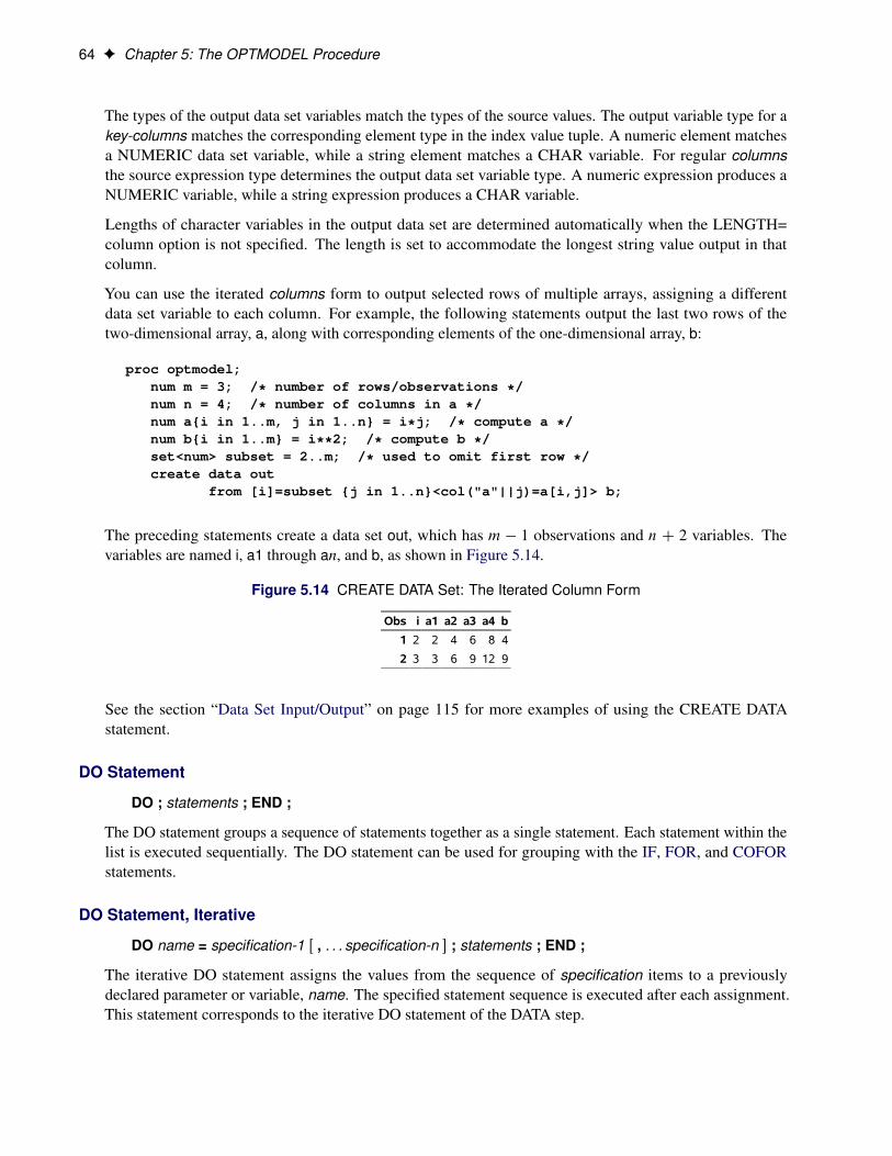
64 F Chapter 5: The OPTMODEL Procedure
The types of the output data set variables match the types of the source values. The output variable type for akey-columns matches the corresponding element type in the index value tuple. A numeric element matchesa NUMERIC data set variable, while a string element matches a CHAR variable. For regular columnsthe source expression type determines the output data set variable type. A numeric expression produces aNUMERIC variable, while a string expression produces a CHAR variable.
Lengths of character variables in the output data set are determined automatically when the LENGTH=column option is not specified. The length is set to accommodate the longest string value output in thatcolumn.
You can use the iterated columns form to output selected rows of multiple arrays, assigning a differentdata set variable to each column. For example, the following statements output the last two rows of thetwo-dimensional array, a, along with corresponding elements of the one-dimensional array, b:
proc optmodel;num m = 3; /* number of rows/observations */num n = 4; /* number of columns in a */num a{i in 1..m, j in 1..n} = i*j; /* compute a */num b{i in 1..m} = i**2; /* compute b */set<num> subset = 2..m; /* used to omit first row */create data out
from [i]=subset {j in 1..n}<col("a"||j)=a[i,j]> b;
The preceding statements create a data set out, which has m � 1 observations and n C 2 variables. Thevariables are named i, a1 through an, and b, as shown in Figure 5.14.
Figure 5.14 CREATE DATA Set: The Iterated Column Form
Obs i a1 a2 a3 a4 b
1 2 2 4 6 8 4
2 3 3 6 9 12 9
See the section “Data Set Input/Output” on page 115 for more examples of using the CREATE DATAstatement.
DO Statement
DO ; statements ; END ;
The DO statement groups a sequence of statements together as a single statement. Each statement within thelist is executed sequentially. The DO statement can be used for grouping with the IF, FOR, and COFORstatements.
DO Statement, Iterative
DO name = specification-1 Œ , . . . specification-n � ; statements ; END ;
The iterative DO statement assigns the values from the sequence of specification items to a previouslydeclared parameter or variable, name. The specified statement sequence is executed after each assignment.This statement corresponds to the iterative DO statement of the DATA step.

Programming Statements F 65
Each specification provides either a single number or a single string value, or a sequence of such values.Each specification takes the following form:
expression Œ WHILE( logic-expression ) j UNTIL( logic-expression ) �
The expression in the specification provides a single value or set of values to assign to the target name.Multiple values can be provided for the loop by giving multiple specification items that are separated bycommas. For example, the following statements output the values 1, 3, and 5:
proc optmodel;number i;do i=1,3,5;
put i;end;
In this case, the same effect can be achieved with a single range expression in place of the explicit list ofvalues, as in the following statements:
proc optmodel;number i;do i=1 to 5 by 2;
put 'value of i assigned by the DO loop = ' i;i=i**2;put 'value of i assigned in the body of the loop = ' i;
end;
The output of these statements is shown in Figure 5.15.
Figure 5.15 DO Loop: Name Parameter Unaffected
value of i assigned by the DO loop = 1 value of i assigned in the body of the loop = 1 value of i assigned by the DO loop = 3 value of i assigned in the body of the loop = 9 value of i assigned by the DO loop = 5 value of i assigned in the body of the loop = 25
Unlike the DATA step, a range expression requires the limit to be specified. Additionally the BY part, if any,must follow the limit expression. Moreover, although the name parameter can be reassigned in the body ofthe loop, the sequence of values that is assigned by the DO loop is unaffected.
The argument expression can also be an expression that returns a set of numbers or strings. For example,the following statements produce the same sequence of values for i as the previous statements but use a setparameter value:
proc optmodel;set s = {1,3,5};number i;do i = s;
put i;end;
Each specification can include a WHILE or UNTIL clause. A WHILE or UNTIL clause applies to theexpression that immediately precedes the clause. The sequence that is specified by an expression can beterminated early by a WHILE or UNTIL clause. A WHILE logic-expression is evaluated for each sequence

66 F Chapter 5: The OPTMODEL Procedure
value before the nested statements. If the logic-expression returns a false (zero or missing) value, then thecurrent sequence is terminated immediately. An UNTIL logic-expression is evaluated for each sequence valueafter the nested statements. The sequence from the current specification is terminated if the logic-expressionreturns a true value (nonzero and nonmissing). After early termination of a sequence due to a WHILE orUNTIL expression, the DO loop execution continues with the next specification, if any.
To demonstrate use of the WHILE clause, the following statements output the values 1, 2, and 3. In this casethe sequence of values from the set s is stopped when the value of i reaches 4.
proc optmodel;set s = {1,2,3,4,5};number i;do i = s while(i NE 4);
put i;end;
DO UNTIL Statement
DO UNTIL ( logic-expression ) ; statements ; END ;
The DO UNTIL loop executes the specified sequence of statements repeatedly until the logic-expression,evaluated after the statements, returns true (a nonmissing nonzero value).
For example, the following statements output the values 1 and 2:
proc optmodel;number i;i = 1;do until (i=3);
put i;i=i+1;
end;
Multiple criteria can be introduced using expression operators, as in the following example:
do until (i=3 and j=7);
For a list of expression operators, see Table 5.10.
DO WHILE Statement
DO WHILE ( logic-expression ) ; statements ; END ;
The DO WHILE loop executes the specified sequence of statements repeatedly as long as the logic-expression,evaluated before the statements, returns true (a nonmissing nonzero value).
For example, the following statements output the values 1 and 2:
proc optmodel;number i;i = 1;do while (i<3);
put i;i=i+1;
end;

Programming Statements F 67
Multiple criteria can be introduced using expression operators, as in the following example:
do while (i<3 and j<7);
For a list of expression operators, see Table 5.10.
DROP Statement
DROP identifier-list ;
The DROP statement causes the solver to ignore a list of constraints, constraint arrays, or constraint arraylocations. The space-delimited identifier-list specifies the names of the dropped constraints. Each constraint,constraint array, or constraint array location is named by an identifier-expression. An entire constraint arrayis dropped if an identifier-expression omits the index for an array name.
The following example statements use the DROP statement:
proc optmodel;var x{1..10};con c1: x[1] + x[2] <= 3;con disp{i in 1..9}: x[i+1] >= x[i] + 0.1;
drop c1; /* drops the c1 constraint */drop disp[5]; /* drops just disp[5] */drop disp; /* drops all disp constraints */
The following line drops both the c1 and disp[5] constraints:
drop c1 disp[5];
Constraints can be added back to the model by using the RESTORE statement.
EXPAND Statement
EXPAND Œ identifier-expression � Œ / options � ;
The EXPAND statement prints the specified constraint, variable, implicit variable, or objective declarationexpressions in the current problem after expanding aggregation operators, substituting the current value forparameters and indices, and resolving constant subexpressions. identifier-expression is the name of a variable,objective, or constraint. If the name is omitted and no options are specified, then all variables, objectives,implicit variables, and undropped constraints in the current problem are printed. The following statementsshow an example EXPAND statement:
proc optmodel;number n=2;var x{1..n};min z1=sum{i in 1..n}(x[i]-i)**2;max z2=sum{i in 1..n}(i-x[i])**3;con c{i in 1..n}: x[i]>=0;fix x[2]=3;expand;
These statements produce the output in Figure 5.16.

68 F Chapter 5: The OPTMODEL Procedure
Figure 5.16 EXPAND Statement Output
Var x[1] Fix x[2] = 3 Maximize z2=(-x[1] + 1)**3 + (-x[2] + 2)**3 Constraint c[1]: x[1] >= 0 Constraint c[2]: x[2] >= 0
Specifying an identifier-expression restricts output to the specified declaration. A non-array name prints onlythe specified item. If an array name is used with a specific index, then information for the specified arraylocation is output. Using an array name without an index restricts output to all locations in the array.
You can use the following options to further control the EXPAND statement output:
SOLVEcauses the EXPAND statement to print the variables, objectives, and constraints in thesame form that would be seen by the solver if a SOLVE statement were executed. Thisincludes any transformations by the PROC OPTMODEL presolver (see the section“Presolver” on page 143). In this form any fixed variables are replaced by their values.Unless an identifier-expression specifies a particular non-array item or array location,the EXPAND output is restricted to only the variables, the constraints, and the currentproblem objective.
The following options restrict the types of declarations output when no specific non-array item or arraylocation is requested. By default, all types of declarations are output. Only the requested declaration typesare output when one or more of the following options are used.
CONSTRAINT | CONrequests the output of undropped constraints.
FIXrequests the output of fixed variables. These variables might have been fixed by the FIXstatement (or by the presolver if the SOLVE option is specified). The FIX option can alsobe used in combination with the name of a variable array to display just the fixed elementsof the array.
IISrestricts the display to items found in the irreducible infeasible set (IIS) after the mostrecent SOLVE performed by the LP solver with the IIS=ON option. The IIS option forthe EXPAND statement can also be used in combination with the name of a variable orconstraint array to display only the elements of the array in the IIS. For more informationabout IIS, see the section “Irreducible Infeasible Set” on page 272.
IMPVARrequests the output of implicit variables referenced in the current problem.
OBJECTIVE | OBJrequests the output of objectives used in the current problem. This includes the currentproblem objective and any objectives referenced as implicit variables.
OMITTED requests the output of variables that are referenced by problem equations but were notincluded in the current USE PROBLEM instance. The OPTMODEL procedure omitsthese variables from the generated problem.

Programming Statements F 69
VARrequests the output of unfixed variables. The VAR option can also be used in combinationwith the name of a variable array to display just the unfixed elements of the array.
For example, you can see the effect of a FIX statement on the problem that is presented to the solver by usingthe SOLVE option. You can modify the previous example as follows:
proc optmodel;number n=2;var x{1..n};min z1=sum{i in 1..n}(x[i]-i)**2;max z2=sum{i in 1..n}(i-x[i])**3;con c{i in 1..n}: x[i]>=0;fix x[2]=3;expand / solve;
These statements produce the output in Figure 5.17.
Figure 5.17 Expansion with Fixed Variable
Var x[1] >= 0 Fix x[2] = 3 Maximize z2=(-x[1] + 1)**3 - 1
Compare the results in Figure 5.17 to those in Figure 5.16. The constraint c[1] has been converted to avariable bound. The subexpression that uses the fixed variable has been resolved to a constant.
FILE Statement
FILE file-specification Œ LRECL=value � ;
The FILE statement selects the current output file for the PUT statement. By default PUT output is sent to theSAS log. Use the FILE statement to manage a group of output files. The specified file is opened for output ifit is not already open. The output file remains open until it is closed with the CLOSEFILE statement.
file-specification names the output file. It can use any of the following forms:
’external-file’specifies the physical name of an external file in quotation marks. The interpretation ofthe filename depends on the operating environment.
file-namespecifies the logical name associated with a file by the FILENAME statement or by theoperating environment. The names PRINT and LOG are reserved to refer to the SASlisting and log files, respectively.
NOTE: Details about the FILENAME statement can be found in SAS Statements: Refer-ence.
( expression )specifies an expression that evaluates to a string that contains the physical name of anexternal file.

70 F Chapter 5: The OPTMODEL Procedure
The LRECL= option sets the line length of the output file. The LRECL= option is ignored if the file is alreadyopen or if the PRINT or LOG file is specified.
The LRECL= value can be specified in these forms:
integerspecifies the desired line length.
identifier-expressionspecifies the name of a numeric parameter that contains the length.
( expression )specifies a numeric expression in parentheses that returns the line length.
The LRECL= value cannot exceed the largest four-byte signed integer, which is 231 � 1.
The following example shows how to use the FILE statement to handle multiple files:
proc optmodel;file 'file.txt' lrecl=80; /* opens file.txt */put 'This is line 1 of file.txt.';file print; /* selects the listing */put 'This goes to the listing.';file 'file.txt'; /* reselects file.txt */put 'This is line 2 of file.txt.';closefile 'file.txt'; /* closes file.txt */file log; /* selects the SAS log */put 'This goes to the log.';
/* using expression to open and write a collection of files */str ofile;num i;num l = 40;do i = 1 to 3;
ofile = ('file' || i || '.txt');file (ofile) lrecl=(l*i);put ('This goes to ' || ofile);closefile (ofile);
end;
The following statements illustrate the usefulness of using a logical name associated with a file by FILENAMEstatement:
proc optmodel;/* assigns a logical name to file.txt *//* see FILENAME statement in *//* SAS Statements: Reference */filename myfile 'file.txt' mod;
file myfile;put 'This is line 3 of file.txt.';closefile myfile;file myfile;put 'This is line 4 of file.txt.';closefile myfile;

Programming Statements F 71
Notice that the FILENAME statement opens the file referenced for append. Therefore, new data are appendedto the end every time the logical name, myfile, is used in the FILE statement.
FIX Statement
FIX identifier-list Œ = expression � ;
The FIX statement causes the solver to treat a list of variables, variable arrays, or variable array locations asfixed in value. The identifier-list consists of one or more variable names separated by spaces. Each memberof the identifier-list is fixed to the same expression. For example, the following statements fix the variables xand y to 3:
proc optmodel;var x, y;num a = 2;fix x y=a+1;
A variable is specified with an identifier-expression (see the section “Identifier Expressions” on page 100).An entire variable array is fixed if the identifier-expression names an array without providing an index. Anew value can be specified with the expression. For example, the following statements fix all locations inarray x to 0 except x[10], which is fixed to 1:
proc optmodel;var x{1..10};fix x = 0;fix x[10] = 1;
If expression is omitted, the variable is fixed at its current value. For example, you can fix some variables tobe their optimal values after the SOLVE statement is invoked. NOTE: The fixed value is equal to the currentvalue for a fixed variable. The fixed value is updated if a new value is assigned to a fixed variable.
The effect of FIX can be reversed by using the UNFIX statement.
FOR Statement
FOR { index-set } statement ;
The FOR statement executes its substatement for each member of the specified index-set . The index set candeclare local dummy parameters. You can reference the value of these parameters in the substatement. Forexample, consider the following statements:
proc optmodel;for {i in 1..2, j in {'a', 'b'}} put i= j=;
These statements produce the output in Figure 5.18.
Figure 5.18 FOR Statement Output
i=1 j=a i=1 j=b i=2 j=a i=2 j=b

72 F Chapter 5: The OPTMODEL Procedure
As another example, the following statements set the current values for variable x to random values between0 and 1:
proc optmodel;var x{1..10};for {i in 1..10}
x[i] = ranuni(-1);
Multiple statements can be controlled by specifying a DO statement group for the substatement.
CAUTION: Avoid modifying the parameters that are used by the FOR or COFOR statement index set fromwithin the substatement. The set value that is used for the left-most index set item is not affected by suchchanges. However, the effect of parameter changes on later index set items cannot be predicted.
IF Statement
IF logic-expression THEN statement Œ ELSE statement � ;
The IF statement evaluates the logical expression and then conditionally executes the THEN or ELSEsubstatements. The substatement that follows the THEN keyword is executed when the logical expressionresult is nonmissing and nonzero. The ELSE substatement, if any, is executed when the logical expressionresult is a missing value or zero. The ELSE part is optional and must immediately follow the THENsubstatement. When IF statements are nested, an ELSE is always matched to the nearest incompleteunmatched IF-THEN. Multiple statements can be controlled by using DO statements with the THEN orELSE substatements.
NOTE: When an IF-THEN statement is used without an ELSE substatement, substatements of the IFstatement are executed when possible as they are entered. Under certain circumstances, such as when anIF statement is nested in a FOR loop, the statement is not executed during interactive input until the nextstatement is seen. By following the IF-THEN statement with an extra semicolon, you can cause it to beexecuted upon submission, since the extra semicolon is handled as a null statement.
LEAVE Statement
LEAVE ;
The LEAVE statement terminates the execution of the entire loop body (iterative DO, DO UNTIL, DOWHILE, FOR, or COFOR) that immediately contains the LEAVE statement. Execution resumes at thestatement that follows the loop. The following example demonstrates a simple use of the LEAVE statement:
proc optmodel;number i, j;do i = 1..5;
do j = 1..4;if i >= 3 and j = 2 then leave;
end;print i j;
end;
The results from these statements are displayed in Figure 5.19.

Programming Statements F 73
Figure 5.19 LEAVE Statement Output
i j
1 4
i j
2 4
i j
3 2
i j
4 2
i j
5 2
For values of i equal to 1 or 2, the inner loop continues uninterrupted, leaving j with a value of 4. For valuesof i equal to 3, 4, or 5, the inner loop terminates early, leaving j with a value of 2.
Null Statement
;
The null statement is treated as a statement in the PROC OPTMODEL syntax, but its execution has no effect.It can be used as a placeholder statement.
PERFORMANCE Statement
PERFORMANCE options ;
The PERFORMANCE statement controls the multithreaded and distributed execution features of PROCOPTMODEL and its solvers. The options that you specify in the PERFORMANCE statement are appliedeach time the statement is executed; they replace any previously specified options. For details about theoptions available for the PERFORMANCE statement, see the section “PERFORMANCE Statement” onpage 19.
Within a COFOR loop, the PERFORMANCE statement controls solvers that are executed subsequently inthe same COFOR iteration. The PERFORMANCE statement cannot specify distributed computing optionsin this context. If the COFOR loop is running in distributed mode, the options affect the solver as it runsin single-machine mode on the remote computing node. In distributed mode, the default NTHREADS=option value is equal to the number of threads on a node in the distributed computing environment. If theCOFOR loop is running in multithreaded mode, the options affect execution of the solver on the machine thatis running PROC OPTMODEL. In multithreaded mode, the default NTHREADS= option value is 1. In eithermode, the NTHREADS= option value is limited to the number of threads in the COFOR loop executionenvironment.
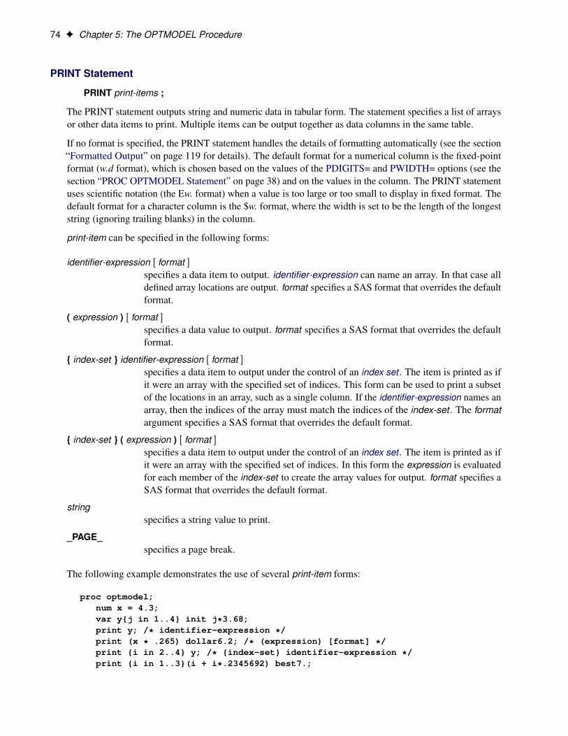
74 F Chapter 5: The OPTMODEL Procedure
PRINT Statement
PRINT print-items ;
The PRINT statement outputs string and numeric data in tabular form. The statement specifies a list of arraysor other data items to print. Multiple items can be output together as data columns in the same table.
If no format is specified, the PRINT statement handles the details of formatting automatically (see the section“Formatted Output” on page 119 for details). The default format for a numerical column is the fixed-pointformat (w.d format), which is chosen based on the values of the PDIGITS= and PWIDTH= options (see thesection “PROC OPTMODEL Statement” on page 38) and on the values in the column. The PRINT statementuses scientific notation (the Ew. format) when a value is too large or too small to display in fixed format. Thedefault format for a character column is the $w. format, where the width is set to be the length of the longeststring (ignoring trailing blanks) in the column.
print-item can be specified in the following forms:
identifier-expression Œ format �specifies a data item to output. identifier-expression can name an array. In that case alldefined array locations are output. format specifies a SAS format that overrides the defaultformat.
( expression ) Œ format �specifies a data value to output. format specifies a SAS format that overrides the defaultformat.
{ index-set } identifier-expression Œ format �specifies a data item to output under the control of an index set . The item is printed as ifit were an array with the specified set of indices. This form can be used to print a subsetof the locations in an array, such as a single column. If the identifier-expression names anarray, then the indices of the array must match the indices of the index-set . The formatargument specifies a SAS format that overrides the default format.
{ index-set } ( expression ) Œ format �specifies a data item to output under the control of an index set . The item is printed as ifit were an array with the specified set of indices. In this form the expression is evaluatedfor each member of the index-set to create the array values for output. format specifies aSAS format that overrides the default format.
stringspecifies a string value to print.
_PAGE_specifies a page break.
The following example demonstrates the use of several print-item forms:
proc optmodel;num x = 4.3;var y{j in 1..4} init j*3.68;print y; /* identifier-expression */print (x * .265) dollar6.2; /* (expression) [format] */print {i in 2..4} y; /* {index-set} identifier-expression */print {i in 1..3}(i + i*.2345692) best7.;
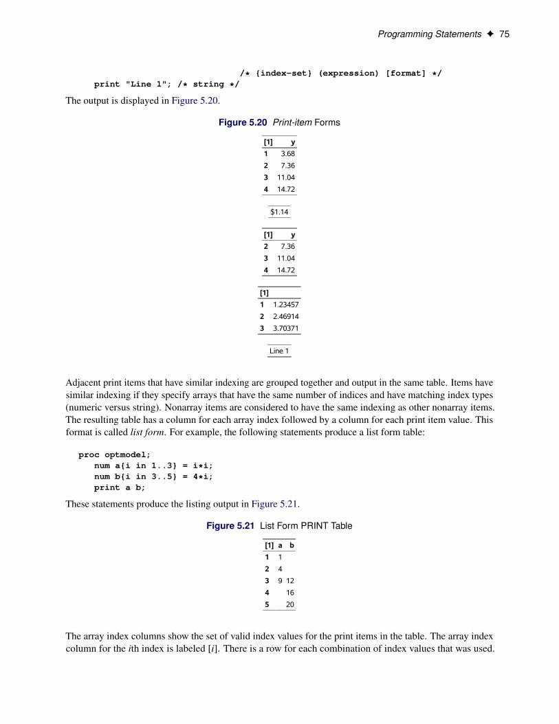
Programming Statements F 75
/* {index-set} (expression) [format] */print "Line 1"; /* string */
The output is displayed in Figure 5.20.
Figure 5.20 Print-item Forms
[1] y
1 3.68
2 7.36
3 11.04
4 14.72
$1.14
[1] y
2 7.36
3 11.04
4 14.72
[1]
1 1.23457
2 2.46914
3 3.70371
Line 1
Adjacent print items that have similar indexing are grouped together and output in the same table. Items havesimilar indexing if they specify arrays that have the same number of indices and have matching index types(numeric versus string). Nonarray items are considered to have the same indexing as other nonarray items.The resulting table has a column for each array index followed by a column for each print item value. Thisformat is called list form. For example, the following statements produce a list form table:
proc optmodel;num a{i in 1..3} = i*i;num b{i in 3..5} = 4*i;print a b;
These statements produce the listing output in Figure 5.21.
Figure 5.21 List Form PRINT Table
[1] a b
1 1
2 4
3 9 12
4 16
5 20
The array index columns show the set of valid index values for the print items in the table. The array indexcolumn for the ith index is labeled [i]. There is a row for each combination of index values that was used.

76 F Chapter 5: The OPTMODEL Procedure
The index values are displayed in sorted ascending order.
The data columns show the array values that correspond to the index values in each row. If a particular arrayindex is invalid or the array location is undefined, then the corresponding table entry is displayed as blankfor numeric arrays and as an empty string for string arrays. If the print items are scalar, then the table has asingle row and no array index columns.
If a table contains a single array print item, the array is two-dimensional (has two indices), and the arrayis dense enough, then the array is shown in matrix form. In this format there is a single index column thatcontains the row index values. The label of this column is blank. This column is followed by a column forevery unique column index value for the array. The latter columns are labeled by the column value. Thesecolumns contain the array values for that particular array column. Table entries that correspond to arraylocations that have invalid or undefined combinations of row and column indices are blank or (for strings)printed as an empty string.
The following statements generate a simple example of matrix output:
proc optmodel;print {i in 1..6, j in i..6} (i*10+j);
The PRINT statement produces the output in Figure 5.22.
Figure 5.22 Matrix Form PRINT Table
1 2 3 4 5 6
1 11 12 13 14 15 16
2 22 23 24 25 26
3 33 34 35 36
4 44 45 46
5 55 56
6 66
The PRINT statement prints single two-dimensional arrays in the form that uses fewer table cells (headingsare ignored). Sparse arrays are normally printed in list form, and dense arrays are normally printed in matrixform. In a PROC OPTMODEL statement, the PMATRIX= option enables you to tune how the PRINTstatement displays a two-dimensional array. The value of this option scales the total number of nonemptyarray elements, which is used to compute the tables cells needed for list form display. Specifying values forthe PMATRIX= option less than 1 causes the list form to be used in more cases, while specifying valuesgreater than 1 causes the matrix form to be used in more cases. If the value is 0, then the list form is alwaysused. The default value of the PMATRIX= option is 1. Changing the default can be done with the RESETOPTIONS statement.
The following statements illustrate how the PMATRIX= option affects the display of the PRINT statement:
proc optmodel;num a{i in 1..6, i..i} = i;num b{i in 1..3, j in 1..3} = i*j;print a;print b;reset options pmatrix=3;print a;reset options pmatrix=0.5;

Programming Statements F 77
print b;
The output is shown in Figure 5.23.
Figure 5.23 PRINT Statement: Effects of PMATRIX= Option
[1] [2] a
1 1 1
2 2 2
3 3 3
4 4 4
5 5 5
6 6 6
b
1 2 3
1 1 2 3
2 2 4 6
3 3 6 9
a
1 2 3 4 5 6
1 1
2 2
3 3
4 4
5 5
6 6
[1] [2] b
1 1 1
1 2 2
1 3 3
2 1 2
2 2 4
2 3 6
3 1 3
3 2 6
3 3 9
From Figure 5.23, you can see that, by default, the PRINT statement tries to make the display compact.However, you can change the default by using the PMATRIX= option.
PROFILE Statement
PROFILE Œ mode � options ;
The PROFILE statement controls the PROC OPTMODEL profiler, which enables you to collect and displaytiming and execution count information for PROC OPTMODEL processing. The profiler can be very usefulfor finding bottlenecks during execution, such as constraints that require large amounts of time duringproblem generation. When the profiler is enabled, PROC OPTMODEL records the time for processing a

78 F Chapter 5: The OPTMODEL Procedure
declaration, the time for executing statements, and the number of times that statements are executed. See“Example 5.7: Sparse Modeling” on page 180 for an example use of the PROFILE statement.
The mode argument specifies the action that the PROFILE statement performs. You can use the followingvalues for mode:
ONenables the profiler. Data are collected until the profiler is disabled or PROC OPTMODELterminates. The profiler is also enabled when no mode is specified in a PROFILEstatement.
OFFdisables the profiler. Note that the profiler is disabled when PROC OPTMODEL beginsexecution.
PRINTprints the current accumulated profiler data. Items for declarations and statements aredisplayed in a table in descending order of their net time. Accumulated data are printedautomatically when PROC OPTMODEL terminates.
The options control how PROC OPTMODEL collects and displays profiler information. Here are the validoptions:
PERCENT=numberrestricts the output for PROFILE PRINT to items whose net times account for at least the specifiedpercentage of total profiled time, total time�number=100. Items that have smaller times are aggregatedinto a single item at the end of the table. You can set this option before the display of profile data, andit does not affect the data collection. The value of number can range from 0 to 100. The default valueis 1.
RESETdiscards accumulated profiler data when the PROFILE statement completes execution. Accumulateddata are retained until they are explicitly reset.
STMTDEPTH=number | ALLallows collection of profiler data for nested statements. With the default option, STMTDEPTH=1,profiler data are collected only for top-level statements. The elapsed time for nested statement timingis included in the top-level statement timing. For example, time for a top-level FOR statementwould include the execution of its substatement. Use the STMTDEPTH= option to profile the nestedstatements individually. The value number specifies the maximum nesting depth at which to profilestatements individually. The nesting depth of a top-level statement is 1. Otherwise the nesting depth ofa statement is one more than the nesting depth of the statement that encloses it, such as a DO, IF, orFOR statement.
For a PROFILE statement within a DO block or DO loop, the statement depth value is interpretedrelative to the enclosing DO statement. For example, specifying STMTDEPTH=1 within a DO blockcauses the top-level statements of the DO block to be profiled. The STMTDEPTH= option is reset toits previous value when the enclosing DO statement completes execution.
The value of number can be an integer between 1 and 32,767. Using the ALL keyword is equivalentto specifying 32,767. Note that profiler timing can add significant overhead. Use a small number tominimize overhead.

Programming Statements F 79
The elapsed time that is required to process an item includes the processing of other profiled items thatit depends on. For example, the processing of a constraint during problem generation might require theevaluation of parameter values. The PROFILE statement reports net time so that the total of profiled timesrepresents actual processing time.
The equation that is used to compute net time is
net time D elapsed time � nested time � wait time
Elapsed time is the elapsed clock time this is required for processing an item. Nested time is the total of theelapsed times that are spent within the same thread to process other profiled items, such as substatements ordeclaration values. Wait time represents the time that a single thread is allocated but idle because it is waitingfor other threads to perform the required processing. The total of net times can exceed the elapsed wall clocktime when multiple threads are used.
PUT Statement
PUT Œ put-items � Œ @ j@@ � ;
The PUT statement writes text data to the current output file. The syntax of the PUT statement in PROCOPTMODEL is similar to the syntax of the PROC IML and DATA step PUT statements. The PUT statementcontains a list of items that specify data for output and provide instructions for formatting the data.
The current output file is initially the SAS log. This can be overridden with the FILE statement. An outputfile can be closed with the CLOSEFILE statement.
Normally the PUT statement outputs the current line after processing all items. Final @ or @@ operatorssuppress this automatic line output and cause the current column position to be retained for use in the nextPUT statement.
put-item can take any of the following forms.
identifier-expression Œ = � Œ format �outputs the value of the parameter or variable that is specified by the identifier-expression.The equal sign (=) causes a name for the location to be printed before each location value.
Normally each item value is printed in a default format. Any leading and trailing blanksin the formatted value are removed, and the value is followed by a blank space. When anexplicit format is specified, the value is printed within the width determined by the format.
name[*] Œ .suffix � Œ = � Œ format �outputs each defined location value for an array parameter. The array name is specified asin the identifier-expression form except that the index list is replaced by an asterisk (*).The equal sign (=) causes a name for the location to be printed before each location valuealong with the actual index values to be substituted for the asterisk.
Each item value normally prints in a default format. Any leading and trailing blanks inthe formatted value are removed, and the value is followed by a blank space. When anexplicit format is specified, the value is printed within the width determined by the format.
( expression ) Œ = � Œ format �outputs the value of the expression enclosed in parentheses. This produces similar resultsto the identifier-expression form except that the equal sign (=) uses the expression to formthe name.

80 F Chapter 5: The OPTMODEL Procedure
’quoted-string’copies the string to the output file.
@integer | identifier-expression | ( expression ) sets the absolute column position within the current line.The literal or expression value determines the new column position.
+integer |identifier-expression|( expression ) sets the relative column position within the current line. Theliteral or expression value determines the amount to update the column position.
/outputs the current line and moves to the first column of the next line.
_PAGE_outputs any pending line data and moves to the top of the next page.
QUIT Statement
QUIT ;
The QUIT statement terminates the OPTMODEL execution. The statement is executed immediately, so itcannot be a nested statement. A QUIT statement is implied when a DATA or PROC statement is read.
READ DATA Statement
READ DATA SAS-data-set Œ NOMISS � INTO Œ Œ set-name = � [ read-key-columns ] � Œ read-columns � ;
The READ DATA statement reads data from a SAS data set into PROC OPTMODEL parameter and variablelocations. The arguments to the READ DATA statement are as follows:
SAS-data-setspecifies the input data set name and options. You can specify the data set name andoptions directly or as the string value of an expression enclosed in parentheses.
set-namespecifies a set parameter in which to save the set of observation key values read from theinput data set.
read-key-columnsprovide the index values for array destinations.
read-columnsspecify the data values to read and the destination locations.
The following example uses the READ DATA statement to copy data set variables j and k from the SAS dataset indata into parameters of the same name. The READ= data set option specifies a password.
proc optmodel;number j, k;read data indata(read=secret) into j k;
Key ColumnsIf any read-key-columns are specified, then the READ DATA statement reads all observations from the inputdata set. If no read-key-columns are specified, then only the first observation of the data set is read. The dataset is closed after reading the requested information.

Programming Statements F 81
Each read-key-column specifies a data set variable that supplies the column value. The values of the specifieddata set variables from each observation are combined into a key tuple. This combination is known as theobservation key. The observation key is used to index array locations specified by the read-columns items.The observation key is expected to be unique for each observation read from the data set.
The syntax for a read-key-column is as follows:
Œ name = � source-name Œ / trim-option �
Each read-key-column specifies an element of the observation key tuple. The source-name specifies the dataset variable name, either as a name or by using a COL expression (as described later for read-columns). Usethe special data set variable name _N_ to refer to the observation’s iteration number, starting at 1.
A local dummy parameter can be created for each read-key-column. You can use the dummy parameter toreference the key tuple element value in subsequent read-columns items. A dummy parameter is createdwhen the read-key-column specifies a name preceding the equal sign (=). The dummy parameter has thespecified name. Also, a dummy parameter is created when the source-name is a nonliteral name and noalternate name has been specified using the equal sign. In this case, the dummy parameter has the same nameas the data set variable.
You can specify a set-name to save the set of observation keys into a set parameter. If the observation keyconsists of a single scalar value, then the set member type must match the scalar type. Otherwise the setmember type must be a tuple with element types that match the corresponding observation key element types.
The READ DATA statement initially assigns an empty set to the target set-name parameter. As observationsare read, a tuple for each observation key is added to the set. A set used to index an array destination in theread-columns can be read at the same time as the array values. Consider a data set, invdata, created by thefollowing statements:
data invdata;input item $ invcount;datalines;
table 100sofa 250chair 80;
The following statements read the data set invdata, which has two variables, item and invcount. The READDATA statement constructs a set of inventory items, Items. At the same time, the parameter locationinvcount[item] is assigned the value of the data set variable invcount in the corresponding observation.
proc optmodel;set<string> Items;number invcount{Items};read data invdata into Items=[item] invcount;print invcount;
The output of these statements is shown in Figure 5.24.
Figure 5.24 READ DATA Statement: Key Column
[1] invcount
chair 80
sofa 250
table 100
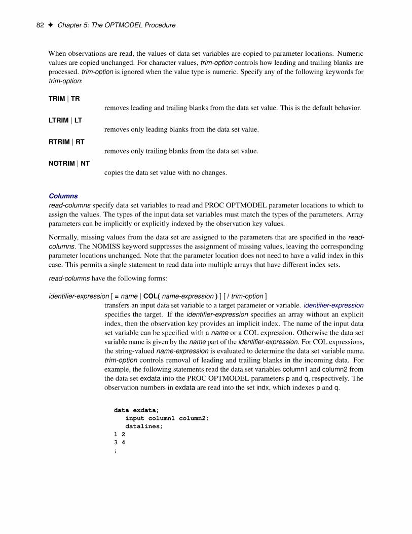
82 F Chapter 5: The OPTMODEL Procedure
When observations are read, the values of data set variables are copied to parameter locations. Numericvalues are copied unchanged. For character values, trim-option controls how leading and trailing blanks areprocessed. trim-option is ignored when the value type is numeric. Specify any of the following keywords fortrim-option:
TRIM j TRremoves leading and trailing blanks from the data set value. This is the default behavior.
LTRIM j LTremoves only leading blanks from the data set value.
RTRIM j RTremoves only trailing blanks from the data set value.
NOTRIM j NTcopies the data set value with no changes.
Columnsread-columns specify data set variables to read and PROC OPTMODEL parameter locations to which toassign the values. The types of the input data set variables must match the types of the parameters. Arrayparameters can be implicitly or explicitly indexed by the observation key values.
Normally, missing values from the data set are assigned to the parameters that are specified in the read-columns. The NOMISS keyword suppresses the assignment of missing values, leaving the correspondingparameter locations unchanged. Note that the parameter location does not need to have a valid index in thiscase. This permits a single statement to read data into multiple arrays that have different index sets.
read-columns have the following forms:
identifier-expression Œ = name j COL( name-expression ) � Œ / trim-option �transfers an input data set variable to a target parameter or variable. identifier-expressionspecifies the target. If the identifier-expression specifies an array without an explicitindex, then the observation key provides an implicit index. The name of the input dataset variable can be specified with a name or a COL expression. Otherwise the data setvariable name is given by the name part of the identifier-expression. For COL expressions,the string-valued name-expression is evaluated to determine the data set variable name.trim-option controls removal of leading and trailing blanks in the incoming data. Forexample, the following statements read the data set variables column1 and column2 fromthe data set exdata into the PROC OPTMODEL parameters p and q, respectively. Theobservation numbers in exdata are read into the set indx, which indexes p and q.
data exdata;input column1 column2;datalines;
1 23 4;

Programming Statements F 83
proc optmodel;number n init 2;set<num> indx;number p{indx}, q{indx};read data exdata into
indx=[_N_] p=column1 q=col("column"||n);print p q;
The output is shown in Figure 5.25.
Figure 5.25 READ DATA Statement: Identifier Expressions
[1] p q
1 1 2
2 3 4
{ index-set } < read-columns >performs the transfers by iterating each column specified by <read-columns> for eachmember of the index-set . If there are n columns and m index set members, then n �mcolumns are generated. The dummy parameters from the index set can be used in thecolumns to generate distinct input data set variable names in the iterated columns, usingCOL expressions. The columns are expanded when the READ DATA statement isexecuted, before any observations are read. This form of read-columns cannot be nested.In other words, the following form of read-columns is NOT allowed:
{ index-set } < { index-set } < read-columns > >
An example that demonstrates the use of the iterated column read-option follows.
You can use an iterated column read-option to read multiple data set variables into the same array. Forexample, a data set might store an entire row of array data in a group of data set variables. The followingstatements demonstrate how to read a data set that contains demand data divided by day:
data dmnd;input loc $ day1 day2 day3 day4 day5;datalines;
East 1.1 2.3 1.3 3.6 4.7West 7.0 2.1 6.1 5.8 3.2;
proc optmodel;set DOW = 1..5; /* days of week, 1=Monday, 5=Friday */set<string> LOCS; /* locations */number demand{LOCS, DOW};read data dmnd
into LOCS=[loc]{d in DOW} < demand[loc, d]=col("day"||d) >;
print demand;
These statements read a set of demand variables named DAY1–DAY5 from each observation, filling in thetwo-dimensional array demand. The output is shown in Figure 5.26.

84 F Chapter 5: The OPTMODEL Procedure
Figure 5.26 Demand Data
demand
1 2 3 4 5
East 1.1 2.3 1.3 3.6 4.7
West 7.0 2.1 6.1 5.8 3.2
RESET OPTIONS Statement
RESET OPTIONS options ;
RESET OPTION options ;
The RESET OPTIONS statement sets PROC OPTMODEL option values or restores them to their defaults.Options can be specified by using the same syntax as in the PROC OPTMODEL statement. The RESETOPTIONS statement provides two extensions to the option syntax. If an option normally requires a value(specified with an equal sign (=) operator), then specifying the option name alone resets it to its defaultvalue. You can also specify an expression enclosed in parentheses in place of a literal value. See the section“OPTMODEL Options” on page 151 for an example.
The RESET OPTIONS statement can be placed inside loops or conditional statements. The statement isapplied each time it is executed.
RESTORE Statement
RESTORE identifier-list ;
The RESTORE statement adds a list of constraints, constraint arrays, or constraint array locations that weredropped by the DROP statement back into the solver model, or includes constraints in a problem wherethey were not previously present. The space-delimited identifier-list specifies the names of the constraints.Each constraint, constraint array, or constraint array location is named by an identifier-expression. An entireconstraint array is restored if an identifier-expression omits the index from an array name. For example, thefollowing statements declare a constraint array and then drop it:
con c{i in 1..4}: x[i] + y[i] <=1;drop c;
The following statement restores the first constraint:
restore c[1];
The following statement restores the second and third constraints:
restore c[2] c[3];
If you want to restore all of the constraints, you can submit the following statement:
restore c;

Programming Statements F 85
SAVE MPS Statement
SAVE MPS SAS-data-set Œ ( OBJECTIVE j OBJ ) name � Œ ( NOOBJECTIVE j NOOBJ ) � ;
The SAVE MPS statement saves the structure and coefficients for a linear programming model into a SASdata set. This data set can be used as input data for the OPTLP or OPTMILP procedure.
NOTE: The OPTMODEL presolver (see the section “Presolver” on page 143) is automatically bypassed sothat the statement saves the original model without eliminating fixed variables, tightening bounds, and so on.
The SAS-data-set argument specifies the output data set name and options. You can specify the data setname and options directly or as the string value of an expression enclosed in parentheses. The output data setuses the MPS format described in Chapter 17, “The MPS-Format SAS Data Set.” The generated data setcontains observations that define different parts of the linear program.
Variables, constraints, and objectives are referenced in the data set by using label text from the corresponding.label suffix value. The default text is based on the name in the model. See the section “Suffixes” on page 131for more details. Labels are limited by default to 32 characters and are abbreviated to fit. You can changethe maximum length for labels by using the MAXLABLEN= option. When needed, a programmaticallygenerated number is added to labels to avoid duplication.
If the OBJECTIVE keyword is used, the objective name becomes the current problem objective. If theNOOBJECTIVE keyword is used or the current problem does not have an objective, then the data set includesa default constant zero objective. Otherwise, the current problem objective is included in the data set.
When an integer variable has been assigned a nondefault branching priority or direction, the MPS data setincludes a BRANCH section. See Chapter 17, “The MPS-Format SAS Data Set,” for more details.
The following statements show an example of the SAVE MPS statement. The model is specified using theOPTMODEL procedure. Then it is saved as the MPS data set MPSData, as shown in Figure 5.27. Next,PROC OPTLP is used to solve the resulting linear program.
proc optmodel;var x >= 0, y >= 0;con c: x >= y;con bx: x <= 2;con by: y <= 1;min obj=0.5*x-y;save mps MPSData;
quit;
proc optlp data=MPSData pout=PrimalOut dout=DualOut;run;

86 F Chapter 5: The OPTMODEL Procedure
Figure 5.27 The MPS Data Set Generated by SAVE MPS Statement
Obs FIELD1 FIELD2 FIELD3 FIELD4 FIELD5 FIELD6
1 NAME MPSData . .
2 ROWS . .
3 N obj . .
4 G c . .
5 L bx . .
6 L by . .
7 COLUMNS . .
8 x obj 0.5 c 1
9 x bx 1.0 .
10 y obj -1.0 c -1
11 y by 1.0 .
12 RHS . .
13 .RHS. bx 2.0 .
14 .RHS. by 1.0 .
15 ENDATA . .
SAVE QPS Statement
SAVE QPS SAS-data-set Œ ( OBJECTIVE j OBJ ) name � Œ ( NOOBJECTIVE j NOOBJ ) � ;
The SAVE QPS statement saves the structure and coefficients for a quadratic programming model into a SASdata set. This data set can be used as input data for the OPTQP procedure.
NOTE: The OPTMODEL presolver (see the section “Presolver” on page 143) is automatically bypassed sothat the statement saves the original model without eliminating fixed variables, tightening bounds, and so on.
The SAS-data-set argument specifies the output data set name and options. You can specify the data setname and options directly or as the string value of an expression enclosed in parentheses. The output dataset uses the QPS format described in Chapter 17. The generated data set contains observations that definedifferent parts of the quadratic program.
Variables, constraints, and objectives are referenced in the data set by using label text from the corresponding.label suffix value. The default text is based on the name in the model. See the section “Suffixes” on page 131for more details. Labels are limited by default to 32 characters and are abbreviated to fit. You can changethe maximum length for labels by using the MAXLABLEN= option. When needed, a programmaticallygenerated number is added to labels to avoid duplication.
If the OBJECTIVE keyword is used, the objective name becomes the current problem objective. If theNOOBJECTIVE keyword is used or the current problem does not have an objective, then the data set includesa default constant zero objective. Otherwise, the current problem objective is included in the data set. Thequadratic coefficients of the objective function appear in the QSECTION section of the output data set.
The following statements show an example of the SAVE QPS statement. The model is specified using theOPTMODEL procedure. Then it is saved as the QPS data set QPSData, as shown in Figure 5.28. Next,PROC OPTQP is used to solve the resulting quadratic program.
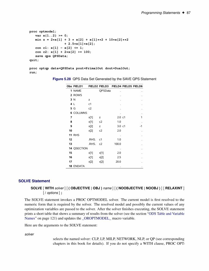
Programming Statements F 87
proc optmodel;var x{1..2} >= 0;min z = 2*x[1] + 3 * x[2] + x[1]**2 + 10*x[2]**2
+ 2.5*x[1]*x[2];con c1: x[1] - x[2] <= 1;con c2: x[1] + 2*x[2] >= 100;save qps QPSData;
quit;
proc optqp data=QPSData pout=PrimalOut dout=DualOut;run;
Figure 5.28 QPS Data Set Generated by the SAVE QPS Statement
Obs FIELD1 FIELD2 FIELD3 FIELD4 FIELD5 FIELD6
1 NAME QPSData . .
2 ROWS . .
3 N z . .
4 L c1 . .
5 G c2 . .
6 COLUMNS . .
7 x[1] z 2.0 c1 1
8 x[1] c2 1.0 .
9 x[2] z 3.0 c1 -1
10 x[2] c2 2.0 .
11 RHS . .
12 .RHS. c1 1.0 .
13 .RHS. c2 100.0 .
14 QSECTION . .
15 x[1] x[1] 2.0 .
16 x[1] x[2] 2.5 .
17 x[2] x[2] 20.0 .
18 ENDATA . .
SOLVE Statement
SOLVE Œ WITH solver � Œ ( OBJECTIVE | OBJ ) name � Œ ( NOOBJECTIVE | NOOBJ ) � Œ RELAXINT �Œ / options � ;
The SOLVE statement invokes a PROC OPTMODEL solver. The current model is first resolved to thenumeric form that is required by the solver. The resolved model and possibly the current values of anyoptimization variables are passed to the solver. After the solver finishes executing, the SOLVE statementprints a short table that shows a summary of results from the solver (see the section “ODS Table and VariableNames” on page 121) and updates the _OROPTMODEL_ macro variable.
Here are the arguments to the SOLVE statement:
solverselects the named solver: CLP, LP, MILP, NETWORK, NLP, or QP (see correspondingchapters in this book for details). If you do not specify a WITH clause, PROC OPT-

88 F Chapter 5: The OPTMODEL Procedure
MODEL chooses a solver that depends on the problem type. Table 5.8 lists the defaultsolver for each problem type.1
Table 5.8 Default Solvers and Algorithms in PROC OPTMODEL
Problem Solver AlgorithmConstraint programming CLP Constraint propagation and backtracking searchLinear programming LP Dual simplexMixed integer linear programming MILP Branch-and-cutGeneral nonlinear programming NLP Interior point NLPQuadratic programming QP Interior point QP
namespecifies the objective to use. This sets the current objective for the problem. You canabbreviate the OBJECTIVE keyword as OBJ. If this argument is not specified, then theproblem objective is unchanged.
NOOBJECTIVE requests that the solver ignore the current objective for the problem and use a constantzero objective instead. This keyword enables the solver to process the current model as afeasibility problem. You can abbreviate the NOOBJECTIVE keyword as NOOBJ.
RELAXINT requests that any integral variables be relaxed to be continuous. RELAXINT can be usedwith linear and nonlinear problems in addition to any solver.
options specifies solver options. You can specify solver options directly only when you use theWITH clause. A list of the options available with the solver is provided in the individualchapters that describe each solver. Table 5.9 lists the available option types. You can usean expression in parentheses in place of a literal option value for numeric and keywordoptions. A string expression is matched to a keyword. OPTMODEL parameters that arechanged by the solver must be specified by a parameter or array option.
Table 5.9 Solver Option Types
Type Syntax ExampleBoolean option | NOoption solve with nlp / NOMULTISTART;Keyword option=name solve with lp / ALGORITHM=PS;Numeric option=number solve with nlp / OPTTOL=1E–4;Parameter option=identifier-expression solve with network / links=(INCLUDE=LINKS) concomp;Array option=array-name Œ .suffix � solve with network / links=(WEIGHT=WEIGHT) tsp;
The SOLVE statement uses the value of the predeclared _SOLVER_OPTIONS_ and _solver_OPTIONS_string parameters to provide default solver options. Any options that are specified by these parameters areadded before options that are specified in the SOLVE statement, with options from _SOLVER_OPTIONS_
1The OPTMODEL procedure never uses the network solver as a default. If the QP solver detects nonconvexity (nonconcavity)for a minimization (maximization) problem, then PROC OPTMODEL calls the NLP solver instead.

Programming Statements F 89
appearing first. These options are included even when the SOLVE statement does not contain a WITH clauseto specify a solver; in this case, solver is the name of the default solver as shown in Table 5.8.
Initially the predeclared string parameters _SOLVER_OPTIONS_ and _solver_OPTIONS_ (for each solver)are empty strings, but you can assign them. You must use keywords or literal values to specify option valuesin these strings. Redundant white space is allowed. For example, the following statements set up some simpledefaults:
_SOLVER_OPTIONS_ = "MAXTIME = 600"; /* options for all solvers */_LP_OPTIONS_ = "PRESOLVER=AGGRESSIVE"; /* options for LP solver */
Optimization techniques that use initial values obtain them from the current values of the optimizationvariables unless the NOINITVAR option is specified. When the solver finishes executing, the current value ofeach optimization variable is replaced by the optimal value found by the solver. These values can then beused as the initial values for subsequent solver invocations.
NOTE: If a solver fails, any currently pending statement is stopped and processing continues with the nextcomplete statement read from the input. For example, if a SOLVE statement that is enclosed in a DO group(see the section “DO Statement” on page 64) fails, then the subsequent statements in the group are notexecuted and processing resumes at the point immediately following the DO group. Neither an infeasibleresult, an unbounded result, nor reaching an iteration limit is considered to be a solver failure.
NOTE: The information that appears in the macro variable _OROPTMODEL_ (see the section “MacroVariable _OROPTMODEL_” on page 159) varies by solver.
NOTE: The RELAXINT keyword is applied immediately before the problem is passed to the solver, afterany processing by the PROC OPTMODEL presolver. So the problem presented to the solver might not beequivalent to the one produced by setting the .RELAX suffix of all variables to a nonzero value. In particular,the bounds of integer variables are still adjusted to be integral, and PROC OPTMODEL’s presolver might useintegrality to tighten bounds further.
STOP Statement
STOP ;
The STOP statement halts the execution of all statements that contain it, including DO statements and othercontrol or looping statements. Execution continues with the next top-level source statement. The followingstatements demonstrate a simple use of the STOP statement:
proc optmodel;number i, j;do i = 1..5;
do j = 1..4;if i = 3 and j = 2 then stop;
end;end;print i j;
The output is shown in Figure 5.29.
Figure 5.29 STOP Statement: Output
i j
3 2

90 F Chapter 5: The OPTMODEL Procedure
When the counters i and j reach 3 and 2, respectively, the STOP statement terminates both loops. Executioncontinues with the PRINT statement.
SUBMIT Statement
SUBMIT arguments Œ / options � ;
SAS statements ;
ENDSUBMIT ;
The SUBMIT statement allows SAS code to be executed before PROC OPTMODEL processing continues.For example, you can use the SUBMIT statement to invoke other SAS procedures to perform analysis or todisplay results. The following statements use PROC SORT to order a list of nodes by decreasing priority; thenodes can be used for further processing:
proc optmodel;set<str> NODES;num priority{NODES};
/* set up priority data... */
/* sort nodes by descending priority */create data temppri from [id] priority;submit;
proc sort;by descending priority;
run;endsubmit;
/* load nodes by priority */str nodesByPri{i in 1..card(NODES)};read data temppri into [_n_] nodesByPri=id;
/* use the sorted list... */
The SUBMIT statement must appear as the last or only statement on a line. It is followed by lines of SASstatements, terminated by the ENDSUBMIT statement on a line of its own. The SAS statements between theSUBMIT and ENDSUBMIT statements are referred to as a SUBMIT block. The SUBMIT block is sent tothe SAS language processor each time the SUBMIT statement is executed.
The SUBMIT block can include SAS global statements and procedure and invocations. Macros are notexpanded until the SUBMIT block is executed. So you can change macro variables to modify the behavior ofthe SUBMIT block each time it is processed.
The arguments list specifies macro variables to initialize before the SUBMIT block is executed. List itemsare separated by spaces. Each of the arguments takes one of the following forms:
namecopies the value of the PROC OPTMODEL parameter name to the macro variable thathas the same name.
name = identifier-expressioncopies the value of the PROC OPTMODEL parameter specified by identifier-expressionto the macro variable name.

Programming Statements F 91
name = number | “string” | ‘string’copies the value of the specified number or string constant to the macro variable name.
name = ( expression )copies the result of evaluating expression to the macro variable name.
The following statements use a SUBMIT argument to modify the output each time the SUBMIT block isinvoked:
for {i in 1..5} do;submit a=i;
%put Value of a is &a..;endsubmit;
end;
The options in the SUBMIT statement are used to retrieve status information after a SUBMIT block isexecuted. Each item in the space-delimited options list has one of the following forms:
OK = identifier-expressionspecifies a PROC OPTMODEL numeric parameter location, identifier-expression, thatis updated to indicate the success of the SUBMIT block execution. The location is setto 1 if execution is successful or 0 if errors are detected. PROC OPTMODEL continuesexecution when the SUBMIT block encounters errors only if the OK= option is specified.
OUT Œ = � output-argumentspecifies a single output-argument for retrieving macro variable values after each execu-tion of the block.
OUT Œ = � ( output-argument )specifies a list of space-delimited output-arguments for retrieving macro variable valuesafter the block is executed.
Each output-argument item specifies a macro variable to copy after the block is executed. Each item takesone of the following two forms:
identifier-expressioncopies the macro variable specified by the name portion of the identifier-expression intothe PROC OPTMODEL parameter location specified by identifier-expression.
identifier-expression = namecopies the macro variable specified by name into the PROC OPTMODEL parameterlocation specified by identifier-expression.
The following statements show how to use the options in the SUBMIT statement to retrieve the result of aSUBMIT block execution:
proc optmodel;num success, syscc;submit / OK = success out syscc;
data example;set notfound;j = i*i;
run;

92 F Chapter 5: The OPTMODEL Procedure
endsubmit;print success syscc;
The DATA step fails, so the success parameter is set to 0 and syscc is set to the error code in the &SYSCCmacro variable. The output is shown in Figure 5.30.
Figure 5.30 SUBMIT Statement Error Handling
success syscc
0 1012
NOTE: The SUBMIT block runs in the same environment that the OPTMODEL procedure is running in. TheSUBMIT block can change the values for options, LIBNAME librefs, FILENAME filerefs, titles, footnotes,and macro variables. The OPTMODEL procedure sees these changes but might not process them until thenext top-level source statement is read.
NOTE: A SUBMIT block can reset the ODS environment of the OPTMODEL procedure. For example, theODS SELECT and EXCLUDE lists could be cleared after the SUBMIT block executes.
NOTE: A SUBMIT statement can appear only in open code. An error message is displayed if the SUBMITstatement is read from a macro. You can avoid this limitation by placing the SUBMIT statement, SUBMITblock, and ENDSUBMIT in a separate file and by using the %INCLUDE statement to include the file in themacro.
UNFIX Statement
UNFIX identifier-list Œ = expression � ;
The UNFIX statement reverses the effect of FIX statements. The solver can vary the specified variables,variable arrays, or variable array locations specified by identifier-list . The identifier-list consists of one ormore variable names separated by spaces.
Each variable name in the identifier-list is an identifier expression (see the section “Identifier Expressions”on page 100). The UNFIX statement affects an entire variable array if the identifier expression omits theindex from an array name. The expression specifies a new initial value that is stored in each element of theidentifier-list .
The following example demonstrates the UNFIX command:
proc optmodel;var x{1..3};fix x; /* fixes entire array to 0 */unfix x[1]; /* x[1] can now be varied again */unfix x[2] = 2; /* x[2] is given an initial value 2 */
/* and can be varied now */unfix x; /* all x indices can now be varied */
After the following statements are executed, the variables x[1] and x[2] are not fixed. They each hold thevalue 4. The variable x[3] is fixed at a value of 2.
proc optmodel;var x{1..3} init 2;num a = 1;fix x;

Details: OPTMODEL Procedure F 93
unfix x[1] x[2]=a+3;
USE PROBLEM Statement
USE PROBLEM identifier-expression ;
The USE PROBLEM programming statement makes the problem specified by the identifier-expression be thecurrent problem. If the problem has not been previously used, the problem is created using the PROBLEMdeclaration corresponding to the name. The problem must have been previously declared.
Details: OPTMODEL Procedure
Named ParametersIn the example described in the section “An Unconstrained Optimization Example” on page 28, all thenumeric constants that describe the behavior of the objective function were specified directly in the objectiveexpression. This is a valid way to formulate the objective expression. However, in many cases it isinconvenient to specify the numeric constants directly. Direct specification of numeric constants can also hidethe structure of the problem that is being solved. The objective expression text would need to be modifiedwhen the numeric values in the problem change. This can be very inconvenient with large models.
In PROC OPTMODEL, you can create named numeric values that behave as constants in expressions. Thesenamed values are called parameters. You can write an expression by using mnemonic parameter names inplace of numeric literals. This produces a clearer formulation of the optimization problem. You can easilymodify the values of parameters, define them in terms of other parameters, or read them from a SAS data set.
The model from this same example can be reformulated in a more general polynomial form, as follows:
data coeff;input c_xx c_x c_y c_xy c_yy;datalines;
1 -1 -2 -1 1;proc optmodel;
var x, y;number c_xx, c_x, c_y, c_xy, c_yy;read data coeff into c_xx c_x c_y c_xy c_yy;min z=c_xx*x**2 + c_x*x + c_y*y + c_xy*x*y + c_yy*y**2;solve;
These statements read the coefficients from a data set, COEFF. The NUMBER statement declares theparameters. The READ DATA statement reads the parameters from the data set. You can apply this modeleasily to coefficients that you have generated by various means.

94 F Chapter 5: The OPTMODEL Procedure
IndexingMany models have large numbers of variables or parameters that can be categorized into families of similarpurpose or behavior. Such families of items can be compactly represented in PROC OPTMODEL by usingindexing. You can use indexing to assign each item in such families to a separate value location.
PROC OPTMODEL indexing is similar to array indexing in the DATA step, but it is more flexible. Indexvalues can be numbers or strings, and are not required to fit into some rigid sequence. PROC OPTMODELindexing is based on index sets, described further in the section “Index Sets” on page 102. For example, thefollowing statement declares an indexed parameter:
number p{1..3};
The construct that follows the parameter name p, “{1..3},” is a simple index set that uses a range expression(see “Range Expression” on page 107). The index set contains the numeric members 1, 2, and 3. Theparameter has distinct value locations for each of the index set members. The first such location is referencedas p[1], the second as p[2], and the third as p[3].
The following statements show an example of indexing:
proc optmodel;number p{1..3};p[1]=5;p[2]=7;p[3]=9;put p[*]=;
The preceding statements produce a line such as the one shown in Figure 5.31 in the log.
Figure 5.31 Indexed Parameter Output
p[1]=5 p[2]=7 p[3]=9
Index sets can also specify local dummy parameters. A dummy parameter can be used as an operand in theexpressions that are controlled by the index set. For example, the assignment statements in the precedingstatements could be replaced by an initialization in the parameter declaration, as follows:
number p{i in 1..3} init 3 + 2*i;
The initialization value of the parameter location p[1] is evaluated with the value of the local dummy parameteri equal to 1. So the initialization expression 3 + 2*i evaluates to 5. Similarly for location p[2], the value of i is2 and the initialization expression evaluates to 7.
The OPTMODEL modeling language supports aggregation operators that combine values of an expressionwhere a local dummy parameter (or parameters) ranges over the members of a set. For example, the SUMaggregation operator combines expression values by adding them together. The following statements output21, since p[1] + p[2] + p[3] = 5 + 7 + 9 = 21:
proc optmodel;number p{i in 1..3} init 3 + 2*i;put (sum{i in 1..3} p[i]);

Types F 95
Aggregation operators like SUM are especially useful in objective expressions because they can combine alarge number of similar expressions into a compact representation. As an example, the following statementsdefine a trivial least squares problem:
proc optmodel;number n init 100000;var x{1..n};min z = sum{i in 1..n}(x[i] - log(i))**2;solve;
The objective function in this case is
z D
nXiD1
.xi � log i/2
Effectively, the objective expression expands to the following large expression:
min z = (x[1] - log(1))**2+ (x[2] - log(2))**2. . .+ (x[99999] - log(99999))**2+ (x[100000] - log(100000))**2;
Even though the problem has 100,000 variables, the aggregation operator SUM enables a compact objectiveexpression.
NOTE: PROC OPTMODEL classifies as mathematically impure any function that returns a different valueeach time it is called. The RAND function, for example, falls into this category. PROC OPTMODELdisallows impure functions inside array index sets, objectives, and constraint expressions. The values ofexpressions that are specified in the declaration of a parameter are resolved in a nondeterministic order duringthreaded problem generation. Therefore, the values are also nondeterministic when these expressions useimpure functions.
TypesIn PROC OPTMODEL, parameters and expressions can have numeric or character values. These correspondto the elementary types named NUMBER and STRING, respectively. The NUMBER type is the same asthe SAS data set numeric type. The NUMBER type includes support for missing values. The STRING typecorresponds to the SAS character type, except that strings can have lengths up to a maximum of 65,534characters (versus 32,767 for SAS character-type variables). The length for a STRING can change as needed.The NUMBER and STRING types together are called the scalar types. You can abbreviate the type names asNUM and STR, respectively.
PROC OPTMODEL also supports set types for parameters and expressions. Sets represent collections ofvalues of a member type, which can be a NUMBER, a STRING, or a vector of scalars (the latter is called atuple and described in the following paragraphs). Members of a set all have the same member type. Membersthat have the same value are stored only once. For example, PROC OPTMODEL stores the set 2, 2, 2 as theset 2.
Specify a set of numbers with SET<NUMBER>. Similarly, specify a set of strings as SET<STRING>.

96 F Chapter 5: The OPTMODEL Procedure
A set can also contain a collection of tuples, all of the same fixed length. A tuple is an ordered collection thatcontains a fixed number of elements. Each element in a tuple contains a scalar value. In PROC OPTMODEL,tuples of length 1 are equivalent to scalars. Two tuples have equal values if the elements at correspondingpositions in each tuple have the same value. Within a set of tuples, the element type at a particular positionin each tuple is the same for all set members. The element types are part of the set type. For example, thefollowing statement declares parts as a set of tuples that have a string in the first element position and anumber in the second element position and then initializes its elements to be <R 1>, <R 2>, <C 1>, and <C2>.
set<string,number> parts = /<R 1> <R 2> <C 1> <C 2>/;
To create a compact model, use sets to take advantage of the structure of the problem being modeled. Forexample, a model might contain various values that specify attributes for each member of a group of suppliers.You could create a set that contains members that represent each supplier. You can then model the attributevalues by using arrays that are indexed by members of the set.
The section “Parameters” on page 96 has more details and examples.
NamesNames are used in the OPTMODEL modeling language to refer to various entities such as parameters orvariables. Names must follow the usual rules for SAS names. Names can be up to 32 characters long and arenot case sensitive. They must be declared before they are used.
Avoid declarations with names that begin with an underscore (_). These names can have special uses inPROC OPTMODEL.
ParametersIn the OPTMODEL modeling language, parameters are named locations that hold constant values. Parameterdeclarations specify the parameter type followed by a list of parameter names to declare. For example, thefollowing statement declares numeric parameters named a and b:
number a, b;
Similarly, the following statements declare a set s of strings, a set n of numbers, and a set sn of tuples:
set<string> s;set<number> n;set<string, number> sn;
You can assign values to parameters in various ways. A parameter can be assigned a value with an assignmentstatement. For example, the following statements assign values to the parameter s, n, and sn in the precedingdeclaration:
s = {'a', 'b', 'c'};n = {1, 2, 3};sn = {<'a',1>, <'b',2>, <'c',3>};

Parameters F 97
Parameter values can also be assigned using a READ DATA statement (see the section “READ DATAStatement” on page 80).
A parameter declaration can provide an explicit value. To specify the value, follow the parameter name withan equal sign (=) and an expression. The value expression can be written in terms of other parameters. Thedeclared parameter takes on a new value each time a parameter that is used in the expression changes. Thisautomatic value update is shown in the following example:
proc optmodel;number pi=4*atan(1);number r;number circum=2*pi*r;r=1;put circum; /* prints 6.2831853072 */r=2;put circum; /* prints 12.566370614 */
The automatic update of parameter values makes it easy to perform “what if” analysis since, after the solverfinds a solution, you can change parameters and reinvoke the solver. You can easily examine the effects ofthe changes on the optimal values.
If you declare a set parameter that has only the SET type specifier, then the element type is determined fromthe initialization expression. If the initialization expression is omitted or if the expression is an empty set,then the set type defaults to SET<NUMBER>. For example, the following statement implicitly declares s1as a set of numbers:
set s1;
The following statement declares s2 as a set of strings:
set s2 = {'A'};
You can declare an array parameter by following the parameter name with an index set specification (see thesection “Index Sets” on page 102). For example, declare an array of 10 numbers as follows:
number c{1..10};
Individual locations of a parameter array can be referred to with an indexing expression. For example, youcan refer to the third location of parameter c as c[3]. Array index sets cannot be specified using a functionsuch as RAND that returns a different value each time it is called.
Parameter names must be declared before they are used. Nonarray names become available at the end of theparameter declaration item. Array names become available after the index set specification. The latter casepermits some forms of recursion in the optional initialization expression that can be supplied for a parameter.
You do not need to assign values to parameters before they are referenced. Most information in PROCOPTMODEL is stored symbolically and resolved when necessary. Values are resolved in certain statements.For example, PROC OPTMODEL resolves a parameter used in the objective during the execution of aSOLVE statement. If no value is available during resolution, then an error is diagnosed.

98 F Chapter 5: The OPTMODEL Procedure
ExpressionsExpressions are grouped into three categories based on the types of values they can produce: logical, set, andscalar (that is, numeric or character).
Logical expressions test for a Boolean (true or false) condition. As in the DATA step, logical operatorsproduce a value equal to either 0 or 1. A value of 0 represents a false condition, while a value of 1 representsa true condition.
Logical expression operators are not allowed in certain contexts due to syntactic considerations. For example,in the VAR statement a logical operator might indicate the start of an option. Enclose a logical expressionin parentheses to use it in such contexts. The difference is illustrated by the output (Figure 5.32) of thefollowing statements, where two variables, x and y, are declared with initial values. The PRINT statementand the EXPAND statement are used to check the initial values and the variable bounds, respectively.
proc optmodel;var x init 0.5 >= 0 <= 1;var y init (0.5 >= 0) <= 1;print x y;expand;
Figure 5.32 Logical Expression in the VAR Statement
x y
0.5 1
Var x >= 0 <= 1 Var y <= 1
Contexts that expect a logical expression also accept numeric expressions. In such cases zero or missingvalues are interpreted as false, and all nonzero nonmissing numeric values are interpreted as true.
Set expressions return a set value. PROC OPTMODEL supports a number of operators that create andmanipulate sets. See the section “OPTMODEL Expression Extensions” on page 103 for a description of thevarious set expressions. Index-set syntax is described in the section “Index Sets” on page 102.
Scalar expressions are similar to the expressions in the DATA step except for PROC OPTMODEL extensions.PROC OPTMODEL provides an IF expression (described in the section “IF-THEN/ELSE Expression” onpage 104). String lengths are assigned dynamically, so there is generally no padding or truncation of stringvalues.
Table 5.10 shows the expression operators from lower to higher precedence (a higher precedence is given alarger number). Operators that have higher precedence are applied in compound expressions before operatorsthat have lower precedence. The table also gives the order of evaluation that is applied when multipleoperators of the same precedence are used together. Operators available in both PROC OPTMODEL and theDATA step have compatible precedences, except that in PROC OPTMODEL the NOT operator has a lowerprecedence than the relational operators. This means that, for example, NOT 1 < 2 is equal to NOT (1 < 2)
(which is 0), rather than (NOT 1) < 2 (which is 1).

Expressions F 99
Table 5.10 Expression Operator Table
Precedence Associativity Operator AlternatesLogic Expression Operators
1 Left to right OR | !
2 Unary OR{index-set}AND{index-set}
3 Left to right AND &
4 Unary NOT � ˆ :
5 Left to right < LT
> GT
<= LE
>= GE
= EQ
�= NE ˆ= :=6 Left to right IN
NOT IN
7 Left to right WITHIN
NOT WITHIN
Set Expression Operators11 IF l THEN s1 ELSE s2
12 Left to right UNION
DIFF
SYMDIFF
13 Unary UNION{index-set}14 Left to right INTER
15 Unary INTER{index-set}16 Left to right CROSS
17 Unary SETOF{index-set}Right to left .. TO
.. e BY TO e BY
Scalar Expression Operators21 IF l THEN e
IF l THEN e1 ELSE e2
22 Left to right || !!
23 Left to right + -
24 Unary SUM{index-set}PROD{index-set}MIN{index-set}MAX{index-set}
25 Left to right * /
26 Unary + -
Right to left ><
<>
** ˆ
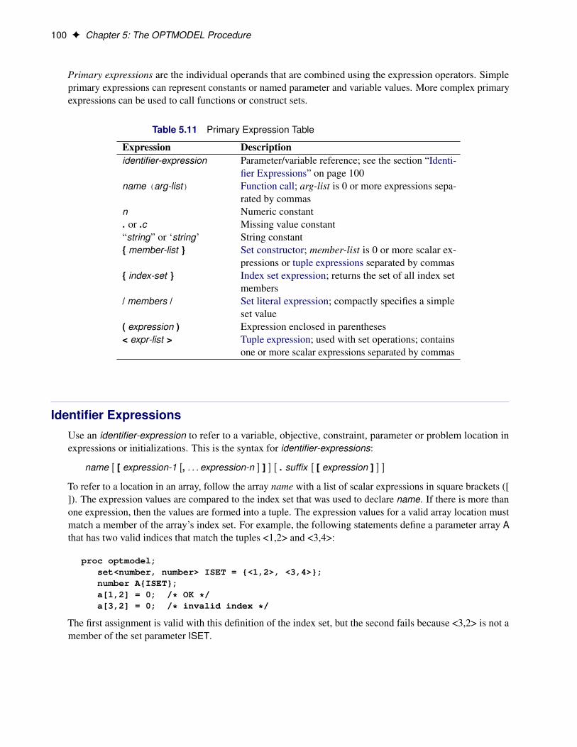
100 F Chapter 5: The OPTMODEL Procedure
Primary expressions are the individual operands that are combined using the expression operators. Simpleprimary expressions can represent constants or named parameter and variable values. More complex primaryexpressions can be used to call functions or construct sets.
Table 5.11 Primary Expression Table
Expression Descriptionidentifier-expression Parameter/variable reference; see the section “Identi-
fier Expressions” on page 100name (arg-list) Function call; arg-list is 0 or more expressions sepa-
rated by commasn Numeric constant. or .c Missing value constant“string” or ‘string’ String constant{ member-list } Set constructor; member-list is 0 or more scalar ex-
pressions or tuple expressions separated by commas{ index-set } Index set expression; returns the set of all index set
members/ members / Set literal expression; compactly specifies a simple
set value( expression ) Expression enclosed in parentheses< expr-list > Tuple expression; used with set operations; contains
one or more scalar expressions separated by commas
Identifier ExpressionsUse an identifier-expression to refer to a variable, objective, constraint, parameter or problem location inexpressions or initializations. This is the syntax for identifier-expressions:
name Œ [ expression-1 Œ, . . . expression-n � ] � Œ . suffix Œ [ expression ] � �
To refer to a location in an array, follow the array name with a list of scalar expressions in square brackets ([]). The expression values are compared to the index set that was used to declare name. If there is more thanone expression, then the values are formed into a tuple. The expression values for a valid array location mustmatch a member of the array’s index set. For example, the following statements define a parameter array Athat has two valid indices that match the tuples <1,2> and <3,4>:
proc optmodel;set<number, number> ISET = {<1,2>, <3,4>};number A{ISET};a[1,2] = 0; /* OK */a[3,2] = 0; /* invalid index */
The first assignment is valid with this definition of the index set, but the second fails because <3,2> is not amember of the set parameter ISET.

Function Expressions F 101
Specify a suffix to refer to auxiliary locations for variables or objectives. For more information, see thesection “Suffixes” on page 131. Certain suffixes can be followed by a numeric index expression that selectsa particular solution saved by the SOLVE statement. For more information about solution indices, see thesection “Multiple Solutions” on page 149.
Function ExpressionsMost functions that can be invoked from the DATA step or the %SYSFUNC macro can be used in PROCOPTMODEL expressions. Certain functions are specific to the DATA step and cannot be used in PROCOPTMODEL. Functions specific to the DATA step include these:
� functions in the LAG, DIF, and DIM families
� functions that access the DATA step program data vector
� functions that access symbol attributes
The CALL statement can invoke SAS library subroutines. These subroutines can read and update the valuesof the parameters and variables that are used as arguments. See the section “CALL Statement” on page 52for an example.
OPTMODEL arrays can be passed to SAS library functions and subroutines using the argument syntax:
OF array-name[*] Œ . suffix �
The array-name is the name of an array symbol. The optional suffix allows auxiliary values to be referenced,as described in section “Suffixes” on page 131.
The OF array form is a compact alternative to listing the array or solution elements explicitly. The OFargument form is resolved into a sequence of arguments, one for each index in the array. The array elementsappear in order of the array’s index set.
As an example, the following statements use the CALL SORTN function to sort the elements of a numericarray:
proc optmodel;number original{i in 1..8} = sin(i);number sorted{i in 1..8} init original[i];call sortn(of sorted[*]);print original sorted;
The output is shown in Figure 5.33. Eight arguments are passed to the SORTN routine. The original columnshows the original order, and the sorted column has the sorted order.

102 F Chapter 5: The OPTMODEL Procedure
Figure 5.33 Sorting Using an OF Array Argument
[1] original sorted
1 0.84147 -0.95892
2 0.90930 -0.75680
3 0.14112 -0.27942
4 -0.75680 0.14112
5 -0.95892 0.65699
6 -0.27942 0.84147
7 0.65699 0.90930
8 0.98936 0.98936
Index SetsAn index set represents a set of combinations of members from the component set expressions. The index setnotation is used in PROC OPTMODEL to describe collections of valid array indices and to specify sets ofvalues with which to perform an operation. Index sets can declare local dummy parameters and can furtherrestrict the set of combinations by a selection expression.
In an index-set specification, the index set consists of one or more index-set-items that are separated bycommas. Each index-set-item can include local dummy parameter declarations. An optional selectionexpression follows the list of index-set-items. The following syntax, which describes an index set, usuallyappears in braces ({}):
index-set-item Œ, . . . index-set-item � Œ : logic-expression �
index-set-item has these forms:
set-expressionname IN set-expression< name-1 Œ, . . . name-n � > IN set-expression
Names that precede the IN keyword in index-set-items declare local dummy parameter names. Dummyparameters correspond to the dummy index variables in mathematical expressions. For example, the followingstatements output the number 385:
proc optmodel;put (sum{i in 1..10} i**2);
The preceding statements evaluate this summation:
10XiD1
i2 D 385
In both the statements and the summation, the index name is i.
The last form of index-set-item in the list can be modified to use the SLICE expression implicitly. See thesection “More on Index Sets” on page 157 for details.
Array index sets cannot be defined using functions that return different values each time the functions arecalled. See the section “Indexing” on page 94 for details.
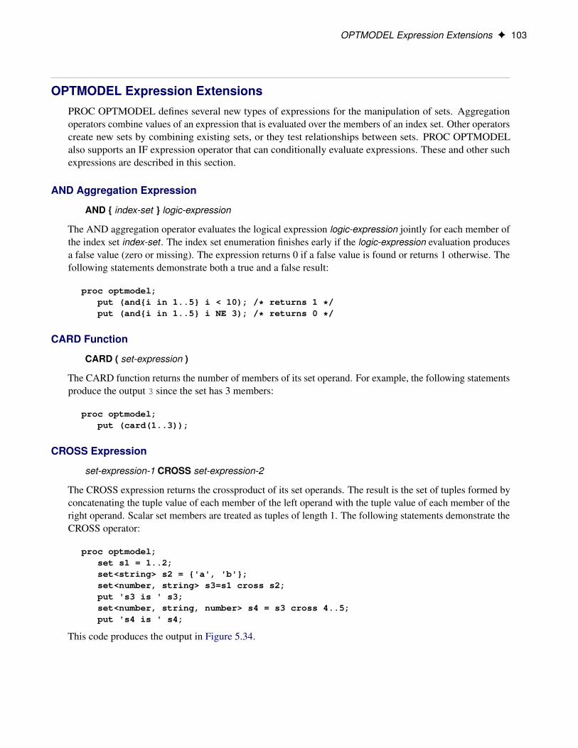
OPTMODEL Expression Extensions F 103
OPTMODEL Expression ExtensionsPROC OPTMODEL defines several new types of expressions for the manipulation of sets. Aggregationoperators combine values of an expression that is evaluated over the members of an index set. Other operatorscreate new sets by combining existing sets, or they test relationships between sets. PROC OPTMODELalso supports an IF expression operator that can conditionally evaluate expressions. These and other suchexpressions are described in this section.
AND Aggregation Expression
AND { index-set } logic-expression
The AND aggregation operator evaluates the logical expression logic-expression jointly for each member ofthe index set index-set . The index set enumeration finishes early if the logic-expression evaluation producesa false value (zero or missing). The expression returns 0 if a false value is found or returns 1 otherwise. Thefollowing statements demonstrate both a true and a false result:
proc optmodel;put (and{i in 1..5} i < 10); /* returns 1 */put (and{i in 1..5} i NE 3); /* returns 0 */
CARD Function
CARD ( set-expression )
The CARD function returns the number of members of its set operand. For example, the following statementsproduce the output 3 since the set has 3 members:
proc optmodel;put (card(1..3));
CROSS Expression
set-expression-1 CROSS set-expression-2
The CROSS expression returns the crossproduct of its set operands. The result is the set of tuples formed byconcatenating the tuple value of each member of the left operand with the tuple value of each member of theright operand. Scalar set members are treated as tuples of length 1. The following statements demonstrate theCROSS operator:
proc optmodel;set s1 = 1..2;set<string> s2 = {'a', 'b'};set<number, string> s3=s1 cross s2;put 's3 is ' s3;set<number, string, number> s4 = s3 cross 4..5;put 's4 is ' s4;
This code produces the output in Figure 5.34.

104 F Chapter 5: The OPTMODEL Procedure
Figure 5.34 CROSS Expression Output
s3 is {<1,'a'>,<1,'b'>,<2,'a'>,<2,'b'>} s4 is {<1,'a',4>,<1,'a',5>,<1,'b',4>,<1,'b',5>,<2,'a',4>,<2,'a',5>,<2,'b',4>,<2,'b',5>}
DIFF Expression
set-expression-1 DIFF set-expression-2
The DIFF operator returns a set that contains the set difference of the left and right operands. The result setcontains values that are members of the left operand but not members of the right operand. The operandsmust have compatible set types. The following statements evaluate and print a set difference:
proc optmodel;put ({1,3} diff {2,3}); /* outputs {1} */
IF-THEN/ELSE Expression
IF logic-expression THEN expression-2 Œ ELSE expression-3 �
The IF-THEN/ELSE expression evaluates the logical expression logic-expression and returns the result ofevaluating the second or third operand expression according to the logical test result. If the logic-expression istrue (nonzero and nonmissing), then the result of evaluating expression-2 is returned. If the logic-expressionis false (zero or missing), then the result of evaluating expression-3 is returned. The other subexpression thatis not selected is not evaluated.
An ELSE clause is matched during parsing with the nearest IF-THEN clause that does not have a matchingELSE. The ELSE clause can be omitted for numeric expressions; the resulting IF-THEN is handled as if adefault ELSE 0 clause were supplied.
Use the IF-THEN/ELSE expression to handle special cases in models. For example, an inventory modelbased on discrete time periods might require special handling for the first or last period. In the followingexample the initial inventory for the first period is assumed to be fixed:
proc optmodel;number T;var inv{1..T}, order{1..T};number sell{1..T};number inv0;. . ./* balance inventory flow */con iflow{i in 1..T}:
inv[i] = order[i] - sell[i] +if i=1 then inv0 else inv[i-1];
. . .
The IF-THEN/ELSE expression in the example models the initial inventory for a time period i. Usually theinventory value is the inventory at the end of the previous period, but for the first time period the inventoryvalue is given by the inv0 parameter. The iflow constraints are linear because the IF-THEN/ELSE testsubexpression does not depend on variables and the other subexpressions are linear.
IF-THEN/ELSE can be used as either a set expression or a scalar expression. The type of expression dependson the subexpression between the THEN and ELSE keywords. The type used affects the parsing of the

OPTMODEL Expression Extensions F 105
subexpression that follows the ELSE keyword because the set form has a lower operator precedence. Forexample, the following two expressions are equivalent because the numeric IF-THEN/ELSE has a higherprecedence than the range operator (..):
IF logic THEN 1 ELSE 2 .. 3
(IF logic THEN 1 ELSE 2) .. 3
But the set form of IF-THEN/ELSE has lower precedence than the range expression operator. So thefollowing two expressions are equivalent:
IF logic THEN 1 .. 2 ELSE 3 .. 4
IF logic THEN (1 .. 2) ELSE (3 .. 4)
The IF-THEN and IF-THEN/ELSE operators always have higher precedence than the logic operators. So, forexample, the following two expressions are equivalent:
IF logic THEN numeric1 < numeric2
(IF logic THEN numeric1) < numeric2
It is best to use parentheses when in doubt about precedence.
IN Expression
expression IN set-expression
expression NOT IN set-expression
The IN expression returns 1 if the value of the left operand is a member of the right operand set. Otherwise,the IN expression returns 0. The NOT IN operator logically negates the returned value. Unlike the DATA step,the right operand is an arbitrary set expression. The left operand can be a tuple expression. The followingexample demonstrates the IN and NOT IN operators:
proc optmodel;set s = 1..10;put (5 in s); /* outputs 1 */put (-1 not in s); /* outputs 1 */set<num, str> t = {<1,'a'>, <2,'b'>, <2,'c'>};put (<2, 'b'> in t); /* outputs 1 */put (<1, 'b'> in t); /* outputs 0 */
Index Set Expression
{ index-set }
The index set expression returns the set of members of an index set. This expression is distinguished from aset constructor (see the section “Set Constructor Expression” on page 108) because it contains a list of setexpressions.
The following statements use an index set with a selection expression that excludes the value 3:

106 F Chapter 5: The OPTMODEL Procedure
proc optmodel;put ({i in 1..5 : i NE 3}); /* outputs {1,2,4,5} */
INTER Expression
set-expression-1 INTER set-expression-2
The INTER operator returns a set that contains the intersection of the left and right operands. This is the setthat contains values that are members of both operand sets. The operands must have compatible set types.
The following statements evaluate and print a set intersection:
proc optmodel;put ({1,3} inter {2,3}); /* outputs {3} */
INTER Aggregation Expression
INTER { index-set } set-expression
The INTER aggregation operator evaluates the set-expression for each member of the index set index-set .The result is the set that contains the intersection of the set of values that were returned by the set-expressionfor each member of the index set. An empty index set causes an expression evaluation error.
The following statements use the INTER aggregation operator to compute the value of {1,2,3,4} \ {2,3,4,5}\ {3,4,5,6}:
proc optmodel;put (inter{i in 1..3} i..i+3); /* outputs {3,4} */
MAX Aggregation Expression
MAX { index-set } expression
The MAX aggregation operator evaluates the numeric expression expression for each member of the indexset index-set . The result is the maximum of the values that are returned by the expression. Missing valuesare handled with the SAS numeric sort order; a missing value is treated as smaller than any nonmissingvalue. If the index set is empty, then the result is the negative number that has the largest absolute valuerepresentable on the machine.
The following example produces the output 0.5:
proc optmodel;put (max{i in 2..5} 1/i);
MIN Aggregation Expression
MIN { index-set } expression
The MIN aggregation operator evaluates the numeric expression expression for each member of the index setindex-set . The result is the minimum of the values that are returned by the expression. Missing values arehandled with the SAS numeric sort order; a missing value is treated as smaller than any nonmissing value. Ifthe index set is empty, then the result is the largest positive number representable on the machine.
The following example produces the output 0.2:

OPTMODEL Expression Extensions F 107
proc optmodel;put (min{i in 2..5} 1/i);
OR Aggregation Expression
OR { index-set } logic-expression
The OR aggregation operator evaluates the logical expression logic-expression for each member of the indexset index-set . The index set enumeration finishes early if the logic-expression evaluation produces a truevalue (nonzero and nonmissing). The result is 1 if a true value is found, or 0 otherwise. The followingstatements demonstrate both a true and a false result:
proc optmodel;put (or{i in 1..5} i = 2); /* returns 1 */put (or{i in 1..5} i = 7); /* returns 0 */
PROD Aggregation Expression
PROD { index-set } expression
The PROD aggregation operator evaluates the numeric expression expression for each member of the indexset index-set . The result is the product of the values that are returned by the expression. This operator isanalogous to the
Qoperator used in mathematical notation. If the index set is empty, then the result is 1.
The following example uses the PROD operator to evaluate a factorial:
proc optmodel;number n = 5;put (prod{i in 1..n} i); /* outputs 120 */
Range Expression
expression-1 .. expression-n Œ BY expression �
The range expression returns the set of numbers from the specified arithmetic progression. The sequenceproceeds from the left operand value up to the right operand limit. The increment between numbers is 1unless a different value is specified with a BY clause. If the increment is negative, then the progression isfrom the left operand down to the right operand limit. The result can be an empty set.
For compatibility with the DATA step iterative DO loop construct, the keyword TO can substitute for therange (..) operator.
The limit value is not included in the resulting set unless it belongs in the arithmetic progression. For example,the following range expression does not include 30:
proc optmodel;put (10..30 by 7); /* outputs {10,17,24} */
The actual numbers that the range expression “f..l by i” produces are in the arithmetic sequence
f; f C i; f C 2i; : : : ; f C ni
where
n D
�l � f
iCp�
�

108 F Chapter 5: The OPTMODEL Procedure
and � represents the relative machine precision. The limit is adjusted to avoid arithmetic roundoff errors.
PROC OPTMODEL represents the set specified by a range expression compactly when the value is stored ina parameter location, used as a set operand of an IN or NOT IN expression, used by an iterative DO loop, orused in an index set. For example, the following expression is evaluated efficiently:
999998.5 IN 1..1000000000
Set Constructor Expression
{ Œ expression-1 Œ , . . . expression-n � � }
The set constructor expression returns the set of the expressions in the member list. Duplicated values areadded to the set only once. A warning message is produced when duplicates are detected. The constructorexpression consists of zero or more subexpressions of the same scalar type or of tuple expressions that matchin length and in element types.
The following statements output a three-member set and warn about the duplicated value 2:
proc optmodel;put ({1,2,3,2}); /* outputs {1,2,3} */
The following example produces a three-member set of tuples, using PROC OPTMODEL parameters andvariables. The output is displayed in Figure 5.35.
proc optmodel;number m = 3, n = 4;var x{1..4} init 1;string y = 'c';put ({<'a', x[3]>, <'b', m>, <y, m/n>});
Figure 5.35 Set Constructor Expression Output
{<'a',1>,<'b',3>,<'c',0.75>}
Set Literal Expression
/ members /
The set literal expression provides compact specification of simple set values. It is equivalent in function tothe set constructor expression but minimizes typing for sets that contain numeric and string constant values.The set members are specified by members, which are literal values. As with the set constructor expression,each member must have the same type.
The following statement specifies a simple numeric set:
/1 2.5 4/
The set contains the members 1, 2.5, and 4. A string set could be specified as follows:
/Miami 'San Francisco' Seattle 'Washington, D.C.'/
This set contains the strings ’Miami’, ’San Francisco’, ’Seattle’, and ’Washington, D.C.’. Youcan specify string values in set literals without quotation marks when the text follows the rules for a SAS
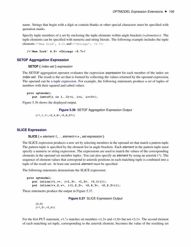
OPTMODEL Expression Extensions F 109
name. Strings that begin with a digit or contain blanks or other special characters must be specified withquotation marks.
Specify tuple members of a set by enclosing the tuple elements within angle brackets (<elements>). Thetuple elements can be specified with numeric and string literals. The following example includes the tupleelements <’New York’, 4.5> and <’Chicago’, -5.7>:
/<'New York' 4.5> <Chicago -5.7>/
SETOF Aggregation Expression
SETOF { index-set } expression
The SETOF aggregation operator evaluates the expression expression for each member of the index setindex-set . The result is the set that is formed by collecting the values returned by the operand expression.The operand can be a tuple expression. For example, the following statements produce a set of tuples ofnumbers with their squared and cubed values:
proc optmodel;put (setof{i in 1..3}<i, i*i, i**3>);
Figure 5.36 shows the displayed output.
Figure 5.36 SETOF Aggregation Expression Output
{<1,1,1>,<2,4,8>,<3,9,27>}
SLICE Expression
SLICE ( < element-1, . . . element-n > , set-expression )
The SLICE expression produces a new set by selecting members in the operand set that match a pattern tuple.The pattern tuple is specified by the element list in angle brackets. Each element in the pattern tuple mustspecify a numeric or string expression. The expressions are used to match the values of the correspondingelements in the operand set member tuples. You can also specify an element by using an asterisk (*). Thesequence of element values that correspond to asterisk positions in each matching tuple is combined into atuple of the result set. At least one asterisk element must be specified.
The following statements demonstrate the SLICE expression:
proc optmodel;put (slice(<1,*>, {<1,3>, <1,0>, <3,1>}));put (slice(<*,2,*>, {<1,2,3>, <2,4,3>, <2,2,5>}));
These statements produce the output in Figure 5.37.
Figure 5.37 SLICE Expression Output
{3,0} {<1,3>,<2,5>}
For the first PUT statement, <1,*> matches set members <1,3> and <1,0> but not <3,1>. The second elementof each matching set tuple, corresponding to the asterisk element, becomes the value of the resulting set

110 F Chapter 5: The OPTMODEL Procedure
member. In the second PUT statement, the values of the first and third elements of the operand set membertuple are combined into a two-position tuple in the result set.
The following statements use the SLICE expression to help compute the transitive closure of a set of tuplesrepresenting a relation by using Warshall’s algorithm. In these statements the set parameter dep represents adirect dependency relation.
proc optmodel;set<str,str> dep = {<'B','A'>, <'C','B'>, <'D','C'>};set<str,str> cl;set<str> cn;cl = dep;cn = (setof{<i,j> in dep} i) inter (setof{<i,j> in dep} j);for {node in cn}
cl = cl union (slice(<*,node>,cl) cross slice(<node,*>,cl));put cl;
The local dummy parameter node in the FOR statement iterates over the set cn of possible intermediatenodes that can connect relations transitively. At the end of each FOR iteration, the set parameter cl containsall tuples from the original set in addition to all transitive tuples found in the current or previous iterations.
The output in Figure 5.38 includes the indirect and direct transitive dependencies from the set dep.
Figure 5.38 Warshall’s Algorithm Output
{<'B','A'>,<'C','B'>,<'D','C'>,<'C','A'>,<'D','B'>,<'D','A'>}
A special form of index-set-item uses the SLICE expression implicitly. See the section “More on Index Sets”on page 157 for details.
SUM Aggregation Expression
SUM { index-set } expression
The SUM aggregation operator evaluates the numeric expression expression for each member in the indexset index-set . The result is the sum of the values that are returned by the expression. If the index set is empty,then the result is 0. This operator is analogous to the
Poperator that is used in mathematical notation. The
following statements demonstrate the use of the SUM aggregation operator:
proc optmodel;put (sum {i in 1..10} i); /* outputs 55 */
SYMDIFF Expression
set-expression-1 SYMDIFF set-expression-2
The SYMDIFF expression returns the symmetric set difference of the left and right operands. The result setcontains values that are members of either the left or right operand but are not members of both operands.The operands must have compatible set types.
The following example demonstrates a symmetric difference:

OPTMODEL Expression Extensions F 111
proc optmodel;put ({1,3} symdiff {2,3}); /* outputs {1,2} */
Tuple Expression
< expression-1 Œ , . . . expression-n � >
A tuple expression represents the value of a member in a set of tuples. Each scalar subexpression insidethe angle brackets represents the value of a tuple element. This form is used only with IN, SETOF, and setconstructor expressions.
The following statements demonstrate the tuple expression:
proc optmodel;put (<1,2,3> in setof{i in 1..2}<i,i+1,i+2>);put ({<1,'a'>, <2,'b'>} cross {<3,'c'>, <4,'d'>});
The first PUT statement checks whether the tuple <1, 2, 3> is a member of a set of tuples. The second PUTstatement outputs the crossproduct of two sets of tuples that are constructed by the set constructor.
These statements produce the output in Figure 5.39.
Figure 5.39 Tuple Expression Output
1 {<1,'a',3,'c'>,<1,'a',4,'d'>,<2,'b',3,'c'>,<2,'b',4,'d'>}
UNION Expression
set-expression-1 UNION set-expression-2
The UNION expression returns the set union of the left and right operands. The result set contains values thatare members of either the left or right operand. The operands must have compatible set types. The followingexample performs a set union:
proc optmodel;put ({1,3} union {2,3}); /* outputs {1,3,2} */
UNION Aggregation Expression
UNION { index-set } set-expression
The UNION aggregation expression evaluates the set-expression for each member of the index set index-set .The result is the set union of the values that are returned by the set-expression. If the index set is empty, thenthe result is an empty set.
The following statements demonstrate a UNION aggregation. The output is the value of {1,2,3,4} [ {2,3,4,5}[ {3,4,5,6}.
proc optmodel;put (union{i in 1..3} i..i+3); /* outputs {1,2,3,4,5,6} */

112 F Chapter 5: The OPTMODEL Procedure
WITHIN Expression
set-expression-1 WITHIN set-expression-2
set-expression NOT WITHIN set-expression
The WITHIN expression returns 1 if the left operand set is a subset of the right operand set and returns 0otherwise. (That is, the operator returns true if every member of the left operand set is a member of theright operand set.) The NOT WITHIN form logically negates the result value. The following statementsdemonstrate the WITHIN and NOT WITHIN operators:
proc optmodel;put ({1,3} within {2,3}); /* outputs 0 */put ({1,3} not within {2,3}); /* outputs 1 */put ({1,3} within {1,2,3}); /* outputs 1 */
Conditions of Optimality
Linear Programming
A standard linear program has the following formulation:
minimize cT xsubject to Ax � b
x � 0
where
x 2 Rn is the vector of decision variablesA 2 Rm�n is the matrix of constraintsc 2 Rn is the vector of objective function coefficientsb 2 Rm is the vector of constraints right-hand sides (RHS)
This formulation is called the primal problem. The corresponding dual problem (see the section “Dual Values”on page 136) is
maximize bT ysubject to AT y � c
y � 0
where y 2 Rm is the vector of dual variables.
The vectors x and y are optimal to the primal and dual problems, respectively, only if there exist primal slackvariables s D Ax � b and dual slack variables w D AT y � c such that the following Karush-Kuhn-Tucker(KKT) conditions are satisfied:
AxC s D b; x � 0; s � 0AT yC w D c; y � 0; w � 0
sT y D 0
wT x D 0

Conditions of Optimality F 113
The first line of equations defines primal feasibility, the second line of equations defines dual feasibility, andthe last two equations are called the complementary slackness conditions.
Nonlinear Programming
To facilitate discussion of optimality conditions in nonlinear programming, you write the general form ofnonlinear optimization problems by grouping the equality constraints and inequality constraints. You alsowrite all the general nonlinear inequality constraints and bound constraints in one form as “�” inequalityconstraints. Thus, you have the following formulation:
minimizex2Rn
f .x/
subject to ci .x/ D 0; i 2 Eci .x/ � 0; i 2 I
where E is the set of indices of the equality constraints, I is the set of indices of the inequality constraints,and m D jE j C jIj.
A point x is feasible if it satisfies all the constraints ci .x/ D 0; i 2 E and ci .x/ � 0; i 2 I. The feasibleregion F consists of all the feasible points. In unconstrained cases, the feasible region F is the entire Rn
space.
A feasible point x� is a local solution of the problem if there exists a neighborhood N of x� such that
f .x/ � f .x�/ for all x 2 N \ F
Further, a feasible point x� is a strict local solution if strict inequality holds in the preceding case; that is,
f .x/ > f .x�/ for all x 2 N \ F
A feasible point x� is a global solution of the problem if no point in F has a smaller function value thanf .x�/; that is,
f .x/ � f .x�/ for all x 2 F
Unconstrained OptimizationThe following conditions hold true for unconstrained optimization problems:
� First-order necessary conditions: If x� is a local solution and f .x/ is continuously differentiable insome neighborhood of x�, then
rf .x�/ D 0
� Second-order necessary conditions: If x� is a local solution and f .x/ is twice continuously differ-entiable in some neighborhood of x�, then r2f .x�/ is positive semidefinite.
� Second-order sufficient conditions: If f .x/ is twice continuously differentiable in some neighbor-hood of x�, rf .x�/ D 0, and r2f .x�/ is positive definite, then x� is a strict local solution.

114 F Chapter 5: The OPTMODEL Procedure
Constrained OptimizationFor constrained optimization problems, the Lagrangian function is defined as follows:
L.x; �/ D f .x/ �Xi2E[I
�ici .x/
where �i ; i 2 E [ I, are called Lagrange multipliers. rxL.x; �/ is used to denote the gradient of theLagrangian function with respect to x, and r2xL.x; �/ is used to denote the Hessian of the Lagrangianfunction with respect to x. The active set at a feasible point x is defined as
A.x/ D E [ fi 2 I W ci .x/ D 0g
You also need the following definition before you can state the first-order and second-order necessaryconditions:
� Linear independence constraint qualification and regular point: A point x is said to satisfy thelinear independence constraint qualification if the gradients of active constraints
rci .x/; i 2 A.x/
are linearly independent. Such a point x is called a regular point.
You now state the theorems that are essential in the analysis and design of algorithms for constrainedoptimization:
� First-order necessary conditions: Suppose that x� is a local minimum and also a regular point. Iff .x/ and ci .x/; i 2 E [ I, are continuously differentiable, there exist Lagrange multipliers �� 2 Rm
such that the following conditions hold:
rxL.x�; ��/ D rf .x�/ �
Xi2E[I
��i rci .x�/ D 0
ci .x�/ D 0; i 2 E
ci .x�/ � 0; i 2 I��i � 0; i 2 I
��i ci .x�/ D 0; i 2 I
The preceding conditions are often known as the Karush-Kuhn-Tucker conditions, or KKT conditionsfor short.
� Second-order necessary conditions: Suppose that x� is a local minimum and also a regular point.Let �� be the Lagrange multipliers that satisfy the KKT conditions. If f .x/ and ci .x/; i 2 E [ I, aretwice continuously differentiable, the following conditions hold:
zTr2xL.x�; ��/z � 0
for all z 2 Rn that satisfy
rci .x�/T z D 0; i 2 A.x�/

Data Set Input/Output F 115
� Second-order sufficient conditions: Suppose there exist a point x� and some Lagrange multipliers�� such that the KKT conditions are satisfied. If
zTr2xL.x�; ��/z > 0
for all z 2 Rn that satisfy
rci .x�/T z D 0; i 2 A.x�/
then x� is a strict local solution.
Note that the set of all such z’s forms the null space of the matrix�rci .x
�/T�i2A.x�/
. Thus, youcan search for strict local solutions by numerically checking the Hessian of the Lagrangian functionprojected onto the null space. For a rigorous treatment of the optimality conditions, see Fletcher (1987)and Nocedal and Wright (1999).
Data Set Input/OutputYou can use the CREATE DATA and READ DATA statements to exchange PROC OPTMODEL datawith SAS data sets. The statements can move data into and out of PROC OPTMODEL parameters andvariables. For example, the following statements use a CREATE DATA statement to save the results from anoptimization into a data set:
proc optmodel;var x;min z = (x-5)**2;solve;create data optdata from xopt=x z;
These statements write a single observation into the data set OPTDATA. The data set contains two variables,xopt and z, and the values contain the optimized values of the PROC OPTMODEL variable x and objective z,respectively. The statement “xopt=x” renames the variable x to xopt.
The group of values held by a data set variable in different observations of a data set is referred to as a column.The READ DATA and CREATE DATA statements specify a set of columns for a data set and define how dataare to be transferred between the columns and PROC OPTMODEL parameters.
Columns in square brackets ([ ]) are handled specially. Such columns are called key columns. Key columnsspecify element values that provide an implicit index for subsequent array columns. The following exampleuses key columns with the CREATE DATA statement to write out variable values from an array:
proc optmodel;set LOCS = {'New York', 'Washington', 'Boston'}; /* locations */set DOW = 1..7; /* day of week */var s{LOCS, DOW} init 1;create data soldata from [location day_of_week]={LOCS, DOW} sale=s;
In this case the optimization variable s is initialized to a value of 1 and is indexed by values from the setparameters LOCS and DOW. The output data set contains an observation for each combination of valuesin these sets. The output data set contains three variables, location, day_of_week, and sale. The data setvariables location and day_of_week save the index element values for the optimization variable s that iswritten in each observation. The data set created is shown in Figure 5.40.
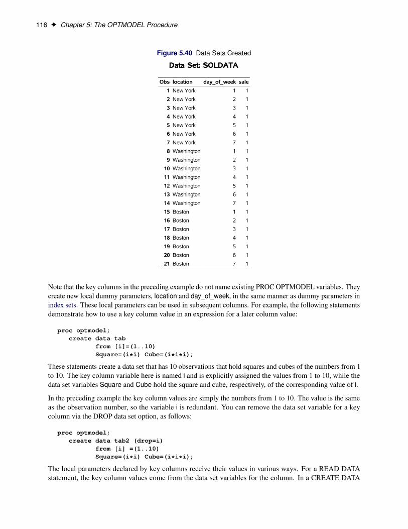
116 F Chapter 5: The OPTMODEL Procedure
Figure 5.40 Data Sets Created
Data Set: SOLDATAData Set: SOLDATA
Obs location day_of_week sale
1 New York 1 1
2 New York 2 1
3 New York 3 1
4 New York 4 1
5 New York 5 1
6 New York 6 1
7 New York 7 1
8 Washington 1 1
9 Washington 2 1
10 Washington 3 1
11 Washington 4 1
12 Washington 5 1
13 Washington 6 1
14 Washington 7 1
15 Boston 1 1
16 Boston 2 1
17 Boston 3 1
18 Boston 4 1
19 Boston 5 1
20 Boston 6 1
21 Boston 7 1
Note that the key columns in the preceding example do not name existing PROC OPTMODEL variables. Theycreate new local dummy parameters, location and day_of_week, in the same manner as dummy parameters inindex sets. These local parameters can be used in subsequent columns. For example, the following statementsdemonstrate how to use a key column value in an expression for a later column value:
proc optmodel;create data tab
from [i]=(1..10)Square=(i*i) Cube=(i*i*i);
These statements create a data set that has 10 observations that hold squares and cubes of the numbers from 1to 10. The key column variable here is named i and is explicitly assigned the values from 1 to 10, while thedata set variables Square and Cube hold the square and cube, respectively, of the corresponding value of i.
In the preceding example the key column values are simply the numbers from 1 to 10. The value is the sameas the observation number, so the variable i is redundant. You can remove the data set variable for a keycolumn via the DROP data set option, as follows:
proc optmodel;create data tab2 (drop=i)
from [i] =(1..10)Square=(i*i) Cube=(i*i*i);
The local parameters declared by key columns receive their values in various ways. For a READ DATAstatement, the key column values come from the data set variables for the column. In a CREATE DATA
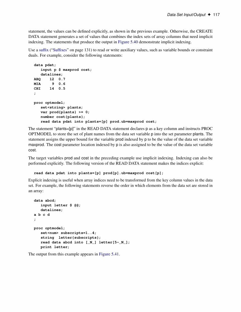
Data Set Input/Output F 117
statement, the values can be defined explicitly, as shown in the previous example. Otherwise, the CREATEDATA statement generates a set of values that combines the index sets of array columns that need implicitindexing. The statements that produce the output in Figure 5.40 demonstrate implicit indexing.
Use a suffix (“Suffixes” on page 131) to read or write auxiliary values, such as variable bounds or constraintduals. For example, consider the following statements:
data pdat;input p $ maxprod cost;datalines;
ABQ 12 0.7MIA 9 0.6CHI 14 0.5;
proc optmodel;set<string> plants;var prod{plants} >= 0;number cost{plants};read data pdat into plants=[p] prod.ub=maxprod cost;
The statement “plants=[p]” in the READ DATA statement declares p as a key column and instructs PROCOPTMODEL to store the set of plant names from the data set variable p into the set parameter plants. Thestatement assigns the upper bound for the variable prod indexed by p to be the value of the data set variablemaxprod. The cost parameter location indexed by p is also assigned to be the value of the data set variablecost.
The target variables prod and cost in the preceding example use implicit indexing. Indexing can also beperformed explicitly. The following version of the READ DATA statement makes the indices explicit:
read data pdat into plants=[p] prod[p].ub=maxprod cost[p];
Explicit indexing is useful when array indices need to be transformed from the key column values in the dataset. For example, the following statements reverse the order in which elements from the data set are stored inan array:
data abcd;input letter $ @@;datalines;
a b c d;
proc optmodel;set<num> subscripts=1..4;string letter{subscripts};read data abcd into [_N_] letter[5-_N_];print letter;
The output from this example appears in Figure 5.41.

118 F Chapter 5: The OPTMODEL Procedure
Figure 5.41 READ DATA Statement: Explicit Indexing
[1] letter
1 d
2 c
3 b
4 a
The following example demonstrates the use of explicit indexing to save sequential subsets of an array inindividual data sets:
data revdata;input month rev @@;datalines;
1 200 2 345 3 362 4 9585 659 6 804 7 487 8 1469 683 10 732 11 652 12 469;
proc optmodel;set m = 1..3;var revenue{1..12};read data revdata into [_N_] revenue=rev;create data qtr1 from [month]=m revenue[month];create data qtr2 from [month]=m revenue[month+3];create data qtr3 from [month]=m revenue[month+6];create data qtr4 from [month]=m revenue[month+9];
Each CREATE DATA statement generates a data set that represents one quarter of the year. Each data setcontains the variables month and revenue. The data set qtr2 is shown in Figure 5.42.
Figure 5.42 CREATE DATA Statement: Explicit Indexing
Obs month revenue
1 1 958
2 2 659
3 3 804
Data set names and options that are used in PROC OPTMODEL statements can also be generated dynamically,by using an expression in parentheses to specify the name and options. The expression must evaluate to astring value with the following form:
Œ libref . � member Œ ( options ) �
Dynamic data set names are useful for processing data sets inside looping statements such as a FOR statement,particularly when the loop contains a SOLVE statement. You can replace the multiple CREATE DATAstatements in the previous example with a single statement in a loop:
proc optmodel;set m = 1..3;var revenue{1..12};read data revdata into [_N_] revenue=rev;for {q in 1..4}

Control Flow F 119
create data ("qtr" || q)from [month]=m revenue[month+(q-1)*3];
Control FlowMost of the control flow statements in PROC OPTMODEL are familiar to users of the DATA step or the IMLprocedure. PROC OPTMODEL supports the IF statement, DO blocks, the iterative DO statement, the DOWHILE statement, and the DO UNTIL statement. You can also use the CONTINUE, LEAVE, and STOPstatements to modify control flow.
PROC OPTMODEL adds the FOR statement. This statement is similar in operation to an iterative DO loop.However, the iteration is performed over the members of an index set. This form is convenient for iterationover all the locations in an array, since the valid array indices are also defined using an index set. For example,the following statements initialize the array parameter A, indexed by i and j, to random values sampled from anormal distribution with mean 0 and variance 1:
proc optmodel;set R=1..10;set C=1..5;number A{R, C};for {i in R, j in C}
A[i, j]=rannor(-1);
The FOR statement provides a convenient way to perform a statement such as the preceding assignmentstatement for each member of a set.
Formatted OutputPROC OPTMODEL provides two primary means of producing formatted output. The PUT statementprovides output of data values with detailed format control. The PRINT statement handles arrays andproduces formatted output in tabular form.
The PUT statement is similar in syntax to the PUT statement in the DATA step and in PROC IML. ThePUT statement can output data to the SAS log, the SAS listing, or an external file. Arguments to the PUTstatement specify the data to output and provide instructions for formatting. The PUT statement providesenough control to create reports within PROC OPTMODEL. However, typically the PUT statement is usedto produce output for debugging or to quickly check data values.
The following example demonstrates some features of the PUT statement:
proc optmodel;number a=1.7, b=2.8;set s={a,b};put a b; /* list output */put a= b=; /* named output */put 'Value A: ' a 8.1 @30 'Value B: ' b 8.; /* formatted */string str='Ratio (A/B) is:';put str (a/b); /* strings and expressions */put s=; /* named set output */
These statements produce the output in Figure 5.43.

120 F Chapter 5: The OPTMODEL Procedure
Figure 5.43 PUT Statement Output
1.7 2.8 a=1.7 b=2.8 Value A: 1.7 Value B: 3 Ratio (A/B) is: 0.6071428571 s={1.7,2.8}
The first PUT statement demonstrates list output. The numeric data values are output in a default format,BEST12., with leading and trailing blanks removed. A blank space is inserted after each data value is output.The second PUT statement uses the equal sign (=) to request that the variable name be output along with theregular list output.
The third PUT statement demonstrates formatted output. It uses the @ operator to position the output in aspecific column. This style of output can be used in report generation. The format specification “8.” causesthe displayed value of parameter b to be rounded.
The fourth PUT statement shows the output of a string value, str. It also outputs the value of an expressionenclosed in parentheses. The final PUT statement outputs a set along with its name.
The default destination for PUT statement output is the SAS log. The FILE and CLOSEFILE statements canbe used to send output to the SAS listing or to an external data file. Multiple files can be open at the sametime. The FILE statement selects the current destination for PUT statement output, and the CLOSEFILEstatement closes the corresponding file. See the section “FILE Statement” on page 69 for more details.
The PRINT statement is designed to output numeric and string data in the form of tables. The PRINTstatement handles the details of formatting automatically. However, the output format can be overridden byPROC OPTMODEL options and through Output Delivery System (ODS) facilities.
The PRINT statement can output array data in a table form that contains a row for each combination of arrayindex values. This form uses columns to display the array index values for each row and uses other columnsto display the value of each requested data item. The following statements demonstrate the table form:
proc optmodel;number square{i in 0..5} = i*i;number recip{i in 1..5} = 1/i;print square recip;
The PRINT statement produces the output in Figure 5.44.
Figure 5.44 PRINT Statement Output (List Form)
[1] square recip
0 0
1 1 1.00000
2 4 0.50000
3 9 0.33333
4 16 0.25000
5 25 0.20000
The first table column, labeled “[1],” contains the index values for the parameters square and recip. Thecolumns that are labeled “square” and “recip” contain the parameter values for each array index. For example,the last row corresponds to the index 5 and the value in the last column is 0.2, which is the value of recip[5].

ODS Table and Variable Names F 121
Note that the first row of the table contains no value in the recip column. Parameter location recip[0] does nothave a valid index, so no value is printed. The PRINT statement does not display variables that are undefinedor have invalid indices. This permits arrays that have similar indexing to be printed together. The sets ofdefined indices in the arrays are combined to generate the set of indices shown in the table.
Also note that the PRINT statement has assigned formats and widths that differ between the square and recipcolumns. The PRINT statement assigns a default fixed-point format to produce the best overall output foreach data column. The format that is selected depends on the PDIGITS= and PWIDTH= options.
The PDIGITS= and PWIDTH= options specify the desired significant digits and formatted width, respectively.If the range of magnitudes is large enough that no suitable format can be found, then the data item is displayedin scientific format. The table in the preceding example displays the last column with five decimal places inorder to display the five significant digits that were requested by the default PDIGITS= value. The squarecolumn, on the other hand, does not need any decimal places.
The PRINT statement can also display two-dimensional arrays in matrix form. If the list following the PRINTstatement contains only a single array that has two index elements, then the array is displayed in matrixform when it is sufficiently dense (otherwise the display is in table form). In this form the left-most columncontains the values of the first index element. The remaining columns correspond to and are labeled by thevalues of the second index element. The following statements print an example of matrix form:
proc optmodel;set R=1..6;set C=1..4;number a{i in R, j in C} = 10*i+j;print a;
The PRINT statement produces the output in Figure 5.45.
Figure 5.45 PRINT Statement Output (Matrix Form)
a
1 2 3 4
1 11 12 13 14
2 21 22 23 24
3 31 32 33 34
4 41 42 43 44
5 51 52 53 54
6 61 62 63 64
In the example the first index element ranges from 1 to 6 and corresponds to the table rows. The second indexelement ranges from 1 to 4 and corresponds to the table columns. Array values can be found based on therow and column values. For example, the value of parameter a[3,2] is 32. This location is found in the tablein the row labeled “3” and the column labeled “2.”
ODS Table and Variable NamesPROC OPTMODEL assigns a name to each table it creates. You can use these names to reference the tablewhen you use the Output Delivery System (ODS) to select tables and create output data sets. The names oftables common to all solvers are listed in Table 5.12. Some solvers can generate additional tables; see the

122 F Chapter 5: The OPTMODEL Procedure
individual solver chapters for more information. For more information about ODS, see SAS Output DeliverySystem: User’s Guide.
Table 5.12 ODS Tables Produced in PROC OPTMODEL
ODS Table Name Description Statement/OptionCoforPerfInfo List of COFOR statement perfor-
mance options and their valuesCOFOR
DerivMethods List of derivatives used by the solver,including the method of computation
SOLVE
OptStatistics Solver-dependent description of theresources required for solution, in-cluding function evaluations andsolver time
SOLVE
PrintTable Specified parameter or variable val-ues
ProblemSummary Description of objective, variables,and constraints
SOLVE
ProfileInfo Detailed timing of statements anddeclarations
PROFILE
SolutionSummary Overview of solution, includingsolver-dependent solution qualityvalues
SOLVE
SolverOptions List of solver options and their values SOLVEPerformanceInfo List of solver performance options
and their valuesSOLVE
Timing Detailed solution timing PERFORMANCE / DE-TAILS
To guarantee that ODS output data sets contain information from all executed statements, use the PERSIST=option in the ODS OUTPUT statement. For details, see SAS Output Delivery System: User’s Guide.NOTE: The SUBMIT statement resets ODS SELECT and EXCLUDE lists.
Table 5.13 lists the variable names of the preceding tables used in the ODS template of the OPTMODELprocedure.
Table 5.13 Variable Names for the ODS Tables Produced in PROC OPTMODEL
ODS Table Name VariablesCoforPerfInfo Label1, cValue1, and nValue1DerivMethods Label1, cValue1, and nValue1OptStatistics Label1, cValue1, and nValue1PrintTable (matrix form) ROW, COL1 – COLnPrintTable (table form) COL1 – COLn, identifier-expression(_suffix)ProblemSummary Label1, cValue1, and nValue1ProfileInfo Item, Line, Column, Count, NetTime, WaitTime, and
PctTimeSolutionSummary Label1, cValue1, and nValue1SolverOptions Label1, cValue1, nValue1, cValue2, and nValue2PerformanceInfo Label1, cValue1, and nValue1Timing Label1, cValue1, nValue1, cValue2, and nValue2

ODS Table and Variable Names F 123
The PRINT statement produces an ODS table named PrintTable. The variable names that are used dependon the display format used. See the section “Formatted Output” on page 119 for details about choosing thedisplay format.
For the PRINT statement with table format, the columns that display array indices are named COL1–COLn,where n is the number of index elements. Columns that display values from identifier expressions are namedusing the expression’s name and suffix. The identifier name becomes the output variable name if no suffix isused. Otherwise the variable name is formed by appending an underscore (_) and the suffix to the identifiername. Columns that display the value of expressions are named COLn, where n is the column number in thetable.
For the PRINT statement with matrix format, the first column has the variable name ROW. The remainingcolumns are named COL1–COLn, where n is the number of distinct column indices. When an ODS tabledisplays values from identifier expressions, a label is generated based on the expression’s name and suffix, asdescribed for column names in the case of table format.
The PRINTLEVEL= option controls the ODS tables produced by the SOLVE and COFOR statements. WhenPRINTLEVEL=0, the statements produce no ODS tables. When PRINTLEVEL=1, the SOLVE statement pro-duces the ODS tables ProblemSummary, SolutionSummary, and PerformanceInfo. When PRINTLEVEL=2,the SOLVE statement produces the ODS tables ProblemSummary, SolverOptions, DerivMethods, Solution-Summary, OptStatistics, and PerformanceInfo. When PRINTLEVEL=1 or 2, the COFOR statement producesthe ODS table CoforPerfInfo.
The PERFORMANCE statement controls additional ODS tables that can be produced by the SOLVE andCOFOR statements. The PerformanceInfo table displays PERFORMANCE statement options that are usedby the SOLVE statement. The CoforPerfInfo table displays PERFORMANCE statement options that areused by the COFOR statement. If you specify the DETAILS option in the PERFORMANCE statement, thenthe SOLVE statement also produces the ODS table Timing. The COFOR statement uses the DETAILS optionto set default performance options with each loop iteration.
The following statements generate several ODS tables and write each table to a SAS data set:
proc optmodel printlevel=2;ods output PrintTable=expt ProblemSummary=exps DerivMethods=exdm
SolverOptions=exso SolutionSummary=exss OptStatistics=exosTiming=exti;
performance details;var x{1..2} >= 0;min z = 2*x[1] + 3 * x[2] + x[1]**2 + 10*x[2]**2
+ 2.5*x[1]*x[2] + x[1]**3;con c1: x[1] - x[2] <= 1;con c2: x[1] + 2*x[2] >= 100;solve;print x;
The data set expt contains the PrintTable table and is shown in Figure 5.46. The variable names are COL1and x.

124 F Chapter 5: The OPTMODEL Procedure
Figure 5.46 PrintTable ODS Table
PrintTablePrintTable
Obs COL1 x
1 1 10.448
2 2 44.776
The data set exps contains the ProblemSummary table and is shown in Figure 5.47. The variable namesare Label1, cValue1, and nValue1. The rows describe the instance, and the description depends on the formof the problem. In most solvers, the rows describe the objective function, variables, and constraints. In thenetwork solver, the rows describe the number of nodes, the number of edges, the directedness of the graph,and the type of problem solved over the graph.
Figure 5.47 ProblemSummary ODS Table
ProblemSummaryProblemSummary
Obs Label1 cValue1 nValue1
1 Objective Sense Minimization .
2 Objective Function z .
3 Objective Type Nonlinear .
4 .
5 Number of Variables 2 2.000000
6 Bounded Above 0 0
7 Bounded Below 2 2.000000
8 Bounded Below and Above 0 0
9 Free 0 0
10 Fixed 0 0
11 .
12 Number of Constraints 2 2.000000
13 Linear LE (<=) 1 1.000000
14 Linear EQ (=) 0 0
15 Linear GE (>=) 1 1.000000
16 Linear Range 0 0
The data set exso contains the SolverOptions table and is shown in Figure 5.48. The variable names areLabel1, cValue1, nValue1, cValue2, and nValue2. The rows, which depend on the solver called by PROCOPTMODEL, list the values taken by each of the solver options. The presence of an asterisk (*) next to anoption indicates that a value has been specified for that option.

ODS Table and Variable Names F 125
Figure 5.48 SolverOptions ODS Table
SolverOptionsSolverOptions
Obs Label1 cValue1 nValue1 cValue2 nValue2
1 ALGORITHM INTERIORPOINT . .
2 FEASTOL 1E-6 0.000001000 .
3 HESSTYPE FULL . .
4 LOGFREQ 1 1.000000 .
5 MAXITER 5000 5000.000000 .
6 MAXTIME I I .
7 OBJLIMIT 1E20 1E20 .
8 OPTTOL 1E-6 0.000001000 .
9 SOLTYPE 1 1.000000 .
10 TIMETYPE REAL . .
The data set exdm contains the DerivMethods table, which displays the methods of derivative computation,and is shown in Figure 5.49. The variable names are Label1, cValue1, and nValue1. The rows, which dependon the derivatives used by the solver, specify the method used to calculate each derivative.
Figure 5.49 DerivMethods ODS Table
DerivMethodsDerivMethods
Obs Label1 cValue1 nValue1
1 Objective Gradient Analytic Formulas .
2 Objective Hessian Analytic Formulas .
The data set exss contains the SolutionSummary table and is shown in Figure 5.50. The variable names areLabel1, cValue1, and nValue1. The rows give an overview of the solution, including the solver chosen, theobjective value, and the solution status. Depending on the values returned by the solver, the SolutionSummarytable might also include some solution quality values such as optimality error and infeasibility. The valuesin the SolutionSummary table appear in the _OROPTMODEL_ macro variable; each solver chapter has asection that describes the solver’s contribution to this macro variable.

126 F Chapter 5: The OPTMODEL Procedure
Figure 5.50 SolutionSummary ODS Table
SolutionSummarySolutionSummary
Obs Label1 cValue1 nValue1
1 Solver NLP .
2 Algorithm Interior Point .
3 Objective Function z .
4 Solution Status Optimal .
5 Objective Value 22623.347101 22623
6 .
7 Optimality Error 5E-7 0.000000500
8 Infeasibility 0 0
9 .
10 Iterations 5 5.000000
11 Presolve Time 0.00 0.000309
12 Solution Time 0.01 0.006643
The data set exos contains the OptStatistics table, which displays the optimization statistics, and is shown inFigure 5.51. The variable names are Label1, cValue1, and nValue1. The rows, which depend on the solvercalled by PROC OPTMODEL, describe the amount of time and the function evaluations that are used bythe solver and associated processing. Times are displayed in seconds of clock or CPU time according to thevalue of the TIMETYPE= option that is used by the solver.
Figure 5.51 OptStatistics ODS Table
OptStatisticsOptStatistics
Obs Label1 cValue1 nValue1
1 Function Evaluations 28 28.000000
2 Gradient Evaluations 28 28.000000
3 Hessian Evaluations 6 6.000000
4 Problem Generation Time 0.00 0.000164
5 Code Generation Time 0.00 0.004873
6 Presolve Time 0.00 0.000309
7 Solution Time 0.01 0.006643
8 Total Time 0.06 0.061089
Problem generation is the process of combining the model with the data into a format that solvers canuse. This includes computing equation coefficients, but it does not include reading data or evaluating otherprogramming statements. Code generation is compiles code for nonlinear equations in the model andperforms other analysis that is needed prior to solver evaluations. The time required for problem generationwill be negligible if the model contains only linear equations. The presolve time in this table includes thetime used by the PROC OPTMODEL presolver and any presolver that is part of the solver. Solution timeis the sum of the times used by the presolvers and the solver. The presolve and solution times also appearin the SolutionSummary table. The OptStatistics table includes a total time, which is the sum of times forproblem generation, code generation, solution, and overhead in the SOLVE statement. Overhead includessolver setup, postprocessing, and ODS table output.

Constraints F 127
The Timing table provides an alternate breakdown of SOLVE statement timing. Times in this table are shownin seconds of clock time. The data set exti, which is shown in Figure 5.52, contains the Timing table dataand statistics. The variable names are Label1, cValue1, nValue1, cValue2, and nValue2. The values presentdepend on the solver and on the context of the SOLVE statement.
Figure 5.52 Timing ODS Table
TimingTiming
Obs Label1 cValue1 nValue1 cValue2 nValue2
1 Problem Generation 0.0001642118 0.00 0.002687733 0.27%
2 OPTMODEL Presolver 0.0003087523 0.00 0.005053498 0.51%
3 Solver Initialization 0.04912925 0.05 0.8041221239 80.41%
4 Code Generation 0.0048727558 0.00 0.0797547444 7.98%
5 Solver 0.0063341265 0.01 0.1036737017 10.37%
6 Solver Postprocessing 0.0002876557 0.00 0.004708199 0.47%
Some of the Timing table values have already been described for the OptStatistics table. Solver initializationtime is overhead in the SOLVE statement before the solver starts. Solver time includes execution of the solverand its associated preprocessor, if any. Solver postprocessing time is overhead in the SOLVE statement afterthe solver has completed. Several table values appear only for a SOLVE statement called within a COFORloop. These values are shown in Table 5.14.
Table 5.14 Solver Timing Values for COFOR Loops
Label DescriptionWaiting for Multiple Threads Time waiting for the required number of threads
to become available on the client machine whenNTHREADS > 1
Waiting for Grid Time waiting for the distributed computing environ-ment to become ready to accept a new problem
Sending to Grid Time to transmit a solver problem description to thedistributed computing environment
Receiving from Grid Time to receive solver results from the distributed com-puting environment
Waiting after Solver Time between solver completion and the resumption ofthe SOLVE statement for processing the results
Grid Overhead Time required for processing in the distributed comput-ing environment that is not included in the precedingtimes
ConstraintsYou can add constraints to a PROC OPTMODEL model. The solver tries to satisfy the specified constraintswhile minimizing or maximizing the objective.
Constraints in PROC OPTMODEL have names. By using the name, you can examine various attributes ofthe constraint, such as the dual value that is returned by the solver (see the section “Suffixes” on page 131 fordetails). A constraint is not allowed to have the same name as any other model component.

128 F Chapter 5: The OPTMODEL Procedure
PROC OPTMODEL provides a default name if none is supplied by the constraint declaration. The predefinedarray _ACON_ provides names for otherwise anonymous constraints. The predefined numeric parameter_NACON_ contains the number of such constraints. The constraints are assigned integer indices in sequence,so _ACON_[1] refers to the first unnamed constraint declared, while _ACON_[_NACON_] refers to the newest.
Consider the following example of a simple model that has a constraint:
proc optmodel;var x, y;min r = x**2 + y**2;con c: x+y >= 1;solve;print x y;
Without the constraint named c, the solver would find the point x D y D 0 that has an objective value of 0.However, the constraint makes this point infeasible. The resulting output is shown in Figure 5.53.
Figure 5.53 Constrained Model Solution
Problem Summary
Objective Sense Minimization
Objective Function r
Objective Type Quadratic
Number of Variables 2
Bounded Above 0
Bounded Below 0
Bounded Below and Above 0
Free 2
Fixed 0
Number of Constraints 1
Linear LE (<=) 0
Linear EQ (=) 0
Linear GE (>=) 1
Linear Range 0
Constraint Coefficients 2
Performance Information
Execution Mode Single-Machine
Number of Threads 4

Constraints F 129
Figure 5.53 continued
Solution Summary
Solver QP
Algorithm Interior Point
Objective Function r
Solution Status Optimal
Objective Value 0.4999995397
Primal Infeasibility 2.3014363E-7
Dual Infeasibility 2.3570226E-7
Bound Infeasibility 0
Duality Gap 1.9574698E-7
Complementarity 0
Iterations 3
Presolve Time 0.00
Solution Time 0.01
x y
0.5 0.5
The solver has found the point where the objective function is minimized in the region x C y � 1. This isactually on the border of the region: the constraint c is active (see the section “Dual Values” on page 136 fordetails).
In the preceding example the constraint c had only a lower bound. You can specify constraints that haveboth upper and lower bounds. For example, replacing the constraint c in the previous example would furtherrestrict the feasible region:
con c: 3 >= x+y >= 1;
PROC OPTMODEL standardizes constraints to collect the expression terms that depend on variables andto separate the expression terms that are constant. When there is a single equality or inequality operator,the separable constant terms are moved to the right operand while the variable terms are moved to the leftoperand. For range constraints, the separable constant terms from the middle expression are subtracted fromthe lower and upper bounds. You can see the standardized constraints with the use of the EXPAND statementin the following example. Consider the following PROC OPTMODEL statements:
proc optmodel;var x{1..3};con b: sum{i in 1..3}(x[i] - i) = 0;expand b;
These statements produce an optimization problem with the following constraint:
(x[1] - 1) + (x[2] - 2) + (x[3] - 3) = 0
The EXPAND statement produces the output in Figure 5.54.
Figure 5.54 Expansion of a Standardized Constraint
Constraint b: x[1] + x[2] + x[3] = 6

130 F Chapter 5: The OPTMODEL Procedure
Here the i separable constant terms in the operand of the SUM operation were moved to the right-hand sideof the constraint. The sum of these i values is 6.
After standardization the constraint expression that contains all the variables is called the body of theconstraint. You can reference the current value of the body expression by attaching the .body suffix to theconstraint name. Similarly, the upper and lower bound expressions can be referenced by using the .ub and .lbsuffixes, respectively. (See the section “Suffixes” on page 131 for more information.)
As a result of standardization, the value of a body expression depends on how the corresponding constraint isentered. The following example demonstrates how using equivalent relational syntax can result in different.body values:
proc optmodel;var x init 1;con c1: x**2 <= 5;con c2: 5 >= x**2;con c3: -x**2 >= -5;con c4: -5 <= -x**2;expand;print c1.body c2.body c3.body c4.body;
The EXPAND and PRINT statements produce the output in Figure 5.55.
Figure 5.55 Expansion and Body Values of Standardized Constraints
Var x Constraint c1: x**2 <= 5 Constraint c2: -x**2 >= -5 Constraint c3: -x**2 >= -5 Constraint c4: --x**2 <= 5
c1.BODY c2.BODY c3.BODY c4.BODY
1 -1 -1 1
CAUTION: Each constraint has an associated dual value (see “Dual Values” on page 136). As a result ofstandardization, the sign of a dual value depends in some instances on the way in which the correspondingconstraint is entered into PROC OPTMODEL. In the case of a minimization objective with one-sidedconstraint g.x/ � L, avoid entering the constraint as L � g.x/. For example, the following statementsproduce a value of 2:
proc optmodel;var x;min o1 = x**2;con c1: x >= 1;solve;print (c1.dual);
Replacing the constraint as follows results in a value of –2:
con c1: 1 <= x;
In the case of a maximization objective with the one-sided constraint g.x/ � U , avoid entering the constraintas U � g.x/.

Suffixes F 131
When a constraint has variables on both sides, the sign of the dual value depends on the direction of theinequality. For example, you can enter the following constraint:
con c1: x**5 - y + 8 <= 5*x + y**2;
This is a � constraint, so c1.dual is nonpositive. If you enter the same constraint as follows, then c1.dual isnonnegative:
con c1: 5*x + y**2 >= x**5 - y + 8;
It is also important to note that the signs of the dual values are negated in the case of maximization. Thefollowing statements output a value of 2:
proc optmodel;var x;min o1 = x**2;con c1: 1 <= x <= 2;solve;print (c1.dual);
Changing the objective function as follows yields the same value of x, but c1.dual now holds the value –2:
max o2 = -x**2;solve;print (c1.dual);
NOTE: A simple bound constraint on a decision variable x can be entered either by using a CONSTRAINTdeclaration or by assigning values to x.lb and x.ub. If you require dual values for simple bound constraints,use the CONSTRAINT declaration.
Constraints that are specified using relational operators can be linear or nonlinear. PROC OPTMODELdetermines the type of constraint automatically by examining the form of the body expression. Subexpressionsthat do not involve variables are treated as constants. Constant subexpressions that are multiplied by or addedto linear subexpressions produce new linear subexpressions. For example, constraint A in the followingstatements is linear:
proc optmodel;var x{1..3};con A: 0.5*(x[1]-x[2]) + x[3] >= 0;
SuffixesYou can use suffixes with identifier-expressions to retrieve and modify various auxiliary values maintainedby the solver. The values of the suffixes can come from expressions in the declaration of the name that issuffixed. For example, the following declaration of variable v provides the values of several suffixes of v atthe same time:
var v >= 0 <= 2 init 1;
The preceding example sets the lower and upper bounds for variable v (that is, v.lb and v.ub, respectively) to0 and 2. The initial value of v is also set to 1. You can use more complex expressions in a declaration, asshown in the following example:

132 F Chapter 5: The OPTMODEL Procedure
num ubound{1..N} init 2;var x{i in 1..N} >= 0 <= ubound[i];
The preceding declaration makes the upper bound value for each element of x equal to the value of theelement in the ubound array with a corresponding index. That is, for each i in 1 to N, x[i ].ub is equal toubound[i ].
The values of the suffixes also come from the solver or from values assigned by assignment, READ DATA,or other statements (see an example in the section “Data Set Input/Output” on page 115). Note that PROCOPTMODEL allows the .lb and .ub suffixes to be assigned after the declaration even when the declarationprovides a value with an expression following >= or <=.
You must use suffixes with names of the appropriate type. For example, the .dual suffix cannot be used withthe name of an objective. In particular, local dummy parameter names cannot have suffixes.
Table 5.15 shows the names of the available suffixes.
Table 5.15 Suffix Names
Name Kind Suffix Modifiable Descriptionany .name No Name text for any non-dummy symbolConstraint .active No Active status in current problemConstraint .block Yes Block ID for decompositionConstraint .body No Current constraint body valueConstraint .dual No Dual value from the solverConstraint .label Yes Label text for the solverConstraint .lb Yes Current lower boundConstraint .status Yes Status information from solverConstraint .ub Yes Current upper boundImplicit Variable .sol No Current solution valueObjective .active No Active status in current problemObjective .sol No Current objective valueObjective .label Yes Label text for the solverProblem .active No Active status of problemProblem .label Yes Label text for the solverVariable .active No Active status in current problemVariable .direction Yes Branching direction for MILPVariable .dual No Alias for .rcVariable .fixed No Fixed statusVariable .label Yes Label text for the solverVariable .lb Yes Lower boundVariable .msinit No Numeric value at the best starting point re-
ported by multistart solverVariable .priority Yes Branching priority for MILP and CLPVariable .rc No Reduced cost (LP) or gradient of Lagrangian
functionVariable .relax Yes Relaxation of integrality restrictionVariable .sol No Current variable valueVariable .sol[i] Yes Saved solution valueVariable .status Yes Status information from solver

Suffixes F 133
Table 5.15 (continued)
Name Kind Suffix Modifiable DescriptionVariable .ub Yes Upper bound
The .sol suffix for a variable, implicit variable, or objective can be used within a declaration to reference thecurrent value of the symbol. It is treated as a constant in such cases. The value is independent of the currentproblem. When the OPTMODEL procedure processes a SOLVE statement, the value is fixed at the startof the SOLVE statement. The .sol suffix can be followed by a positive integer solution index to refer to aparticular solution that the SOLVE statement returns. See the section “Multiple Solutions” on page 149 formore information about accessing multiple solutions from the solver. Each problem tracks saved solutionvalues separately. Outside of declarations, a variable, implicit variable, or objective name with the .sol suffixand no solution index is equivalent to the unsuffixed name.
The .status suffix reports status information from the solver. Currently, only the LP solver provides statusinformation. The .status suffix takes on the same character values that are found in the _STATUS_ variable ofthe PRIMALOUT and DUALOUT data sets for the OPTLP procedure, including values set by the IIS= option.See the section “Variable and Constraint Status” on page 271 and the section “Irreducible Infeasible Set” onpage 272, both in Chapter 7, “The Linear Programming Solver,” for more information. For other solvers, the.status values default to a single blank character.
If you choose to modify the .status suffix for a variable or constraint, the assigned suffix value can be a singlecharacter or an empty string. The LP solver rejects invalid status characters. Blank or empty strings aretreated as new row or column entries for the purpose of “warm starting” the solver.
The .active suffix reports the current activity status for names in the problem. The value is 1 if the element isactive or 0 otherwise. A PROBLEM name is considered active if it is the current problem (that is, it wasselected by the most recent USE PROBLEM statement). A constraint is considered active if it is included inthe current problem and not dropped. An objective is considered active if it is the selected objective for thecurrent problem. A variable is considered active if it is included in the current problem, independent of thefixed status.
The .fixed suffix reports the fixed status of a variable. The value is 1 if the variable is fixed using the FIXstatement for the current problem or 0 otherwise. Variables that are not included in the current problem aretreated as unfixed.
The .msinit suffix reports the numeric value of a variable at the best starting point, as reported by the NLPsolver when the MULTISTART option is specified. If the solver does not report a best starting point, thenthe value is missing. The value is tracked independently for each problem to support multiple subproblems.See the section “Multistart” on page 512 in Chapter 10, “The Nonlinear Programming Solver,” for moreinformation.
The .block suffix identifies the subproblem for constraints when used with the METHOD=USER optionof the decomposition algorithm. The value must be numeric and is initially assigned a missing value. Aconstraint with a missing value for the .block suffix is part of the master problem. Otherwise constraintsbelong to the same subproblem if and only if they have the same .block suffix values. See Chapter 15, “TheDecomposition Algorithm,” for more information.
The .label suffix represents the text passed to the solver to identify a variable, constraint, or objective. Somesolvers can display this label in their output. The maximum text length passed to the solver is controlled bythe MAXLABLEN= option. The default text is based on the name in the model, abbreviated to fit within

134 F Chapter 5: The OPTMODEL Procedure
MAXLABLEN. For example, a model variable x[1] would be labeled “x[1]”. This label text can be reassigned.The .label suffix value is also used to create MPS labels stored in the output data set for the SAVE MPS andSAVE QPS statements.
The .name suffix represents the name of a symbol as a text string. The .name suffix can be used with anydeclared name except for local dummy parameters. This suffix is primarily useful when applied to problemsymbols (see the section “Problem Symbols” on page 150), since the .name suffix returns the name ofthe referenced symbol, not the problem symbol name. The name text is based on the name in the model,abbreviated to fit in 256 characters.
Suffixed names can be used wherever a parameter name is accepted, provided only the value is required.However, you are not allowed to change the value of certain suffixes. Table 5.15 marks these suffixes as notmodifiable. Suffixed names that are used as a target in an assignment or READ DATA statement must bemodifiable.
The following statements formulate a trivial linear programming problem. The objective value is unbounded,which is reported after the execution of the SOLVE statement. The PRINT statements illustrate the corre-sponding default auxiliary values. This is shown in Figure 5.56.
proc optmodel;var x, y;min z = x + y;con c: x + 2*y <= 3;solve;print x.lb x.ub x.status x.sol;print y.lb y.ub y.status y.sol;print c.lb c.ub c.body c.dual;
Figure 5.56 Using a Suffix: Retrieving Auxiliary Values
x.LB x.UB x.STATUS x.SOL
-1.7977E+308 1.7977E+308 I 0
y.LB y.UB y.STATUS y.SOL
-1.7977E+308 1.7977E+308 I 0
c.LB c.UB c.BODY c.DUAL
-1.7977E+308 3 0 .
Next, continue to submit the following statements to change the default bounds and solve again. The outputis shown in Figure 5.57.
x.lb=0;y.lb=0;c.lb=1;solve;print x.lb x.ub x.status x.sol;print y.lb y.ub y.status y.sol;print c.lb c.ub c.body c.dual;

Integer Variable Suffixes F 135
Figure 5.57 Using a Suffix: Modifying Auxiliary Values
x.LB x.UB x.STATUS x.SOL
0 1.7977E+308 L 0
y.LB y.UB y.STATUS y.SOL
0 1.7977E+308 B 0.5
c.LB c.UB c.BODY c.DUAL
1 3 1 0.5
NOTE: Spaces are significant. The form NAME. TAG is treated as a SAS format name followed by the tagname, not as a suffixed identifier. The forms NAME.TAG, NAME . TAG, and NAME .TAG (note the locationof spaces) are interpreted as suffixed references.
Integer Variable SuffixesThe suffixes .relax, .priority, and .direction are applicable to integer variables.
For an integer variable x, setting x.relax to a nonzero, nonmissing value relaxes the integrality restriction.The value of x.relax is read as either 1 or 0, depending on whether or not integrality is relaxed. This suffix isignored for noninteger variables.
The value that is contained in x.priority sets the priority of an integer variable x for use with branching inthe MILP solver or selection in the CLP solvers. This value can be any nonnegative, nonmissing number.The default value is 0, which indicates default branching priority. Variables with positive .priority values areassigned greater priority than the default. Variables with the highest .priority values are assigned the highestpriority. Variables with the same .priority value are assigned the same branching priority.
The value of x.direction assigns a branching direction to an integer variable x. This value should be an integerin the range –1 to 3. A noninteger value in this range is rounded on assignment. The default value is 0. Thesignificance of each integer is found in Table 5.16.
Table 5.16 Branching Directions
Value Direction–1 Round down to nearest integer0 Default1 Round up to nearest integer2 Round to nearest integer3 Round to closest presolved bound
Suppose the solver branches next on an integer variable x whose last LP relaxation solution is 3.3. Supposealso that after passing through the presolver, the lower bound of x is 0 and the upper bound of x is 10. If thevalue in x.direction is –1 or 2, then the solver sets x to 3 for the next iteration. If the value in x.direction is 1,then the solver sets x to 4. If the value in x.direction is 3, then the solver sets x to 0.

136 F Chapter 5: The OPTMODEL Procedure
The MPS data set created by the SAVE MPS statement (“SAVE MPS Statement” on page 85) includes aBRANCH section if any nondefault .priority or .direction values have been specified for integer variables.
Dual ValuesA dual value is associated with each constraint. To access the dual value of a constraint, use the constraintname followed by the suffix .dual.
For linear programming problems, the dual value associated with a constraint is also known as the dual price(also called the shadow price). The shadow price is usually interpreted economically as the rate at which theoptimal value changes with respect to a change in some right-hand side that represents a resource supply ordemand requirement.
For nonlinear programming problems, the dual values correspond to the values of the optimal Lagrangemultipliers. For more details about duality in nonlinear programming, see Bazaraa, Sherali, and Shetty(1993).
From the dual value associated with the constraint, you can also tell whether the constraint is active or not. Aconstraint is said to be active (tight at a point) if it holds with equality at that point. It can be informative toidentify active constraints at the optimal point and check their corresponding dual values. Relaxing the activeconstraints might improve the objective value.
Background on Duality in Mathematical Programming
For a minimization problem, there exists an associated problem with the following property: any feasiblesolution to the associated problem provides a lower bound for the original problem, and conversely anyfeasible solution to the original problem provides an upper bound for the associated problem. The originaland the associated problems are referred to as the primal and the dual problem, respectively. More specifically,consider the primal problem,
minimizex
f .x/
subject to ci .x/ D 0; i 2 Eci .x/ � 0; i 2 Lci .x/ � 0; i 2 G
where E , L, and G denote the sets of equality, � inequality, and � inequality constraints, respectively.Variables x 2 Rn are called the primal variables. The Lagrangian function of the primal problem is defined as
L.x; �; �; �/ D f .x/ �Xi2E
�ici .x/ �Xi2L
�ici .x/ �Xi2G
�ici .x/
where �i 2 R, �i � 0, and �i � 0. By convention, the Lagrange multipliers for inequality constraints haveto be nonnegative. Hence �, ��, and � correspond to the Lagrange multipliers in the preceding Lagrangianfunction. It can be seen that the Lagrangian function is a linear combination of the objective function andconstraints of the primal problem.
The Lagrangian function plays a fundamental role in nonlinear programming. It is used to define theoptimality conditions that characterize a local minimum of the primal problem. It is also used to formulatethe dual problem of the preceding primal problem. To this end, consider the following dual function:
d.�; �; �/ D infxL.x; �; �; �/
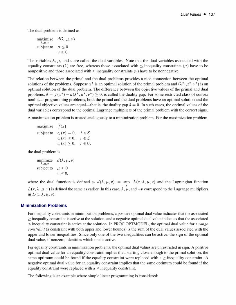
Dual Values F 137
The dual problem is defined as
maximize�;�;�
d.�; �; �/
subject to � � 0
� � 0:
The variables �, �, and � are called the dual variables. Note that the dual variables associated with theequality constraints (�) are free, whereas those associated with � inequality constraints (�) have to benonpositive and those associated with � inequality constraints (�) have to be nonnegative.
The relation between the primal and the dual problems provides a nice connection between the optimalsolutions of the problems. Suppose x� is an optimal solution of the primal problem and .��; ��; ��/ is anoptimal solution of the dual problem. The difference between the objective values of the primal and dualproblems, ı D f .x�/ � d.��; ��; ��/ � 0, is called the duality gap. For some restricted class of convexnonlinear programming problems, both the primal and the dual problems have an optimal solution and theoptimal objective values are equal—that is, the duality gap ı D 0. In such cases, the optimal values of thedual variables correspond to the optimal Lagrange multipliers of the primal problem with the correct signs.
A maximization problem is treated analogously to a minimization problem. For the maximization problem
maximizex
f .x/
subject to ci .x/ D 0; i 2 Eci .x/ � 0; i 2 Lci .x/ � 0; i 2 G;
the dual problem is
minimize�;�;�
d.�; �; �/
subject to � � 0
� � 0:
where the dual function is defined as d.�; �; �/ D supx
L.x; �; �; �/ and the Lagrangian function
L.x; �; �; �/ is defined the same as earlier. In this case, �, �, and �� correspond to the Lagrange multipliersin L.x; �; �; �/.
Minimization Problems
For inequality constraints in minimization problems, a positive optimal dual value indicates that the associated� inequality constraint is active at the solution, and a negative optimal dual value indicates that the associated� inequality constraint is active at the solution. In PROC OPTMODEL, the optimal dual value for a rangeconstraint (a constraint with both upper and lower bounds) is the sum of the dual values associated with theupper and lower inequalities. Since only one of the two inequalities can be active, the sign of the optimaldual value, if nonzero, identifies which one is active.
For equality constraints in minimization problems, the optimal dual values are unrestricted in sign. A positiveoptimal dual value for an equality constraint implies that, starting close enough to the primal solution, thesame optimum could be found if the equality constraint were replaced with a � inequality constraint. Anegative optimal dual value for an equality constraint implies that the same optimum could be found if theequality constraint were replaced with a � inequality constraint.
The following is an example where simple linear programming is considered:

138 F Chapter 5: The OPTMODEL Procedure
proc optmodel;var x, y;min z = 6*x + 7*y;con
4*x + y >= 5,-x - 3*y <= -4,x + y <= 4;
solve;print x y;expand _ACON_ ;print _ACON_.dual _ACON_.body;
The PRINT statements generate the output shown in Figure 5.58.
Figure 5.58 Dual Values in Minimization Problem: Display
Problem Summary
Objective Sense Minimization
Objective Function z
Objective Type Linear
Number of Variables 2
Bounded Above 0
Bounded Below 0
Bounded Below and Above 0
Free 2
Fixed 0
Number of Constraints 3
Linear LE (<=) 2
Linear EQ (=) 0
Linear GE (>=) 1
Linear Range 0
Constraint Coefficients 6
Performance Information
Execution Mode Single-Machine
Number of Threads 1

Dual Values F 139
Figure 5.58 continued
Solution Summary
Solver LP
Algorithm Dual Simplex
Objective Function z
Solution Status Optimal
Objective Value 13
Primal Infeasibility 0
Dual Infeasibility 0
Bound Infeasibility 0
Iterations 4
Presolve Time 0.00
Solution Time 0.00
x y
1 1
Constraint _ACON_[1]: 4*x + y >= 5 Constraint _ACON_[2]: - x - 3*y <= -4 Constraint _ACON_[3]: x + y <= 4
[1] _ACON_.DUAL _ACON_.BODY
1 1 5
2 -2 -4
3 0 2
It can be seen that the first and second constraints are active, with dual values 1 and –2. Continue to submitthe following statements. Notice how the objective value is changed in Figure 5.59.
_ACON_[1].lb = _ACON_[1].lb - 1;solve;_ACON_[2].ub = _ACON_[2].ub + 1;solve;

140 F Chapter 5: The OPTMODEL Procedure
Figure 5.59 Dual Values in Minimization Problem: Interpretation
Problem Summary
Objective Sense Minimization
Objective Function z
Objective Type Linear
Number of Variables 2
Bounded Above 0
Bounded Below 0
Bounded Below and Above 0
Free 2
Fixed 0
Number of Constraints 3
Linear LE (<=) 2
Linear EQ (=) 0
Linear GE (>=) 1
Linear Range 0
Constraint Coefficients 6
Performance Information
Execution Mode Single-Machine
Number of Threads 1
Solution Summary
Solver LP
Algorithm Dual Simplex
Objective Function z
Solution Status Optimal
Objective Value 12
Primal Infeasibility 0
Dual Infeasibility 0
Bound Infeasibility 0
Iterations 4
Presolve Time 0.00
Solution Time 0.00

Dual Values F 141
Figure 5.59 continued
Problem Summary
Objective Sense Minimization
Objective Function z
Objective Type Linear
Number of Variables 2
Bounded Above 0
Bounded Below 0
Bounded Below and Above 0
Free 2
Fixed 0
Number of Constraints 3
Linear LE (<=) 2
Linear EQ (=) 0
Linear GE (>=) 1
Linear Range 0
Constraint Coefficients 6
Performance Information
Execution Mode Single-Machine
Number of Threads 1
Solution Summary
Solver LP
Algorithm Dual Simplex
Objective Function z
Solution Status Optimal
Objective Value 10
Primal Infeasibility 0
Dual Infeasibility 0
Bound Infeasibility 0
Iterations 4
Presolve Time 0.00
Solution Time 0.00
The change is just as the dual values imply. After the first constraint is relaxed by one unit, the objectivevalue is improved by one unit. For the second constraint, the relaxation and improvement are one unit andtwo units, respectively.
NOTE: The signs of dual values produced by PROC OPTMODEL depend, in some instances, on the way inwhich the corresponding constraints are entered. See the section “Constraints” on page 127 for details.
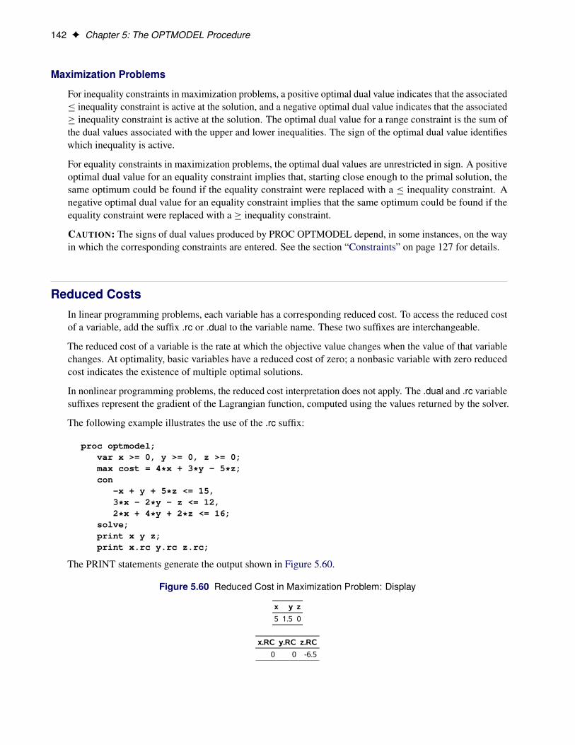
142 F Chapter 5: The OPTMODEL Procedure
Maximization Problems
For inequality constraints in maximization problems, a positive optimal dual value indicates that the associated� inequality constraint is active at the solution, and a negative optimal dual value indicates that the associated� inequality constraint is active at the solution. The optimal dual value for a range constraint is the sum ofthe dual values associated with the upper and lower inequalities. The sign of the optimal dual value identifieswhich inequality is active.
For equality constraints in maximization problems, the optimal dual values are unrestricted in sign. A positiveoptimal dual value for an equality constraint implies that, starting close enough to the primal solution, thesame optimum could be found if the equality constraint were replaced with a � inequality constraint. Anegative optimal dual value for an equality constraint implies that the same optimum could be found if theequality constraint were replaced with a � inequality constraint.
CAUTION: The signs of dual values produced by PROC OPTMODEL depend, in some instances, on the wayin which the corresponding constraints are entered. See the section “Constraints” on page 127 for details.
Reduced CostsIn linear programming problems, each variable has a corresponding reduced cost. To access the reduced costof a variable, add the suffix .rc or .dual to the variable name. These two suffixes are interchangeable.
The reduced cost of a variable is the rate at which the objective value changes when the value of that variablechanges. At optimality, basic variables have a reduced cost of zero; a nonbasic variable with zero reducedcost indicates the existence of multiple optimal solutions.
In nonlinear programming problems, the reduced cost interpretation does not apply. The .dual and .rc variablesuffixes represent the gradient of the Lagrangian function, computed using the values returned by the solver.
The following example illustrates the use of the .rc suffix:
proc optmodel;var x >= 0, y >= 0, z >= 0;max cost = 4*x + 3*y - 5*z;con
-x + y + 5*z <= 15,3*x - 2*y - z <= 12,2*x + 4*y + 2*z <= 16;
solve;print x y z;print x.rc y.rc z.rc;
The PRINT statements generate the output shown in Figure 5.60.
Figure 5.60 Reduced Cost in Maximization Problem: Display
x y z
5 1.5 0
x.RC y.RC z.RC
0 0 -6.5

Presolver F 143
In this example, x and y are basic variables, while z is nonbasic. The reduced cost of z is –6.5, which impliesthat increasing z from 0 to 1 decreases the optimal value from 24.5 to 18.
PresolverPROC OPTMODEL includes a simple presolver that processes linear constraints to produce tighter boundson variables. The presolver can reduce the number of variables and constraints that are presented to the solver.These changes can result in reduced solution times.
Linear constraints that involve only a single variable are converted into variable bounds. The presolver theneliminates redundant linear constraints for which variable bounds force the constraint to always be satisfied.Tightly bounded variables where upper and lower bounds are within the range specified by the VARFUZZ=option (see the section “PROC OPTMODEL Statement” on page 38) are automatically fixed to the averageof the bounds. The presolver also eliminates variables that are fixed by the user or by the presolver.
The presolver can infer tighter variable bounds from linear constraints when all variables in the constraintor all but one variable have known bounds. For example, when given the following PROC OPTMODELdeclarations, the presolver can use the inferred bounds x � 7 and y � 4 to remove the constraint c2:
proc optmodel;var x >= 3;var y >= 0;con c: x + y <= 7;con c2: x + 2*y <= 15; /* redundant */
The presolver makes multiple passes and rechecks linear constraints after bounds are tightened for thereferenced variables. The number of passes is controlled by the PRESOLVER= option. After the passes arefinished, the presolver attempts to fix the value of all variables that are not used in the updated objectiveand constraints. The current value of such a variable is used if the value lies between the variable’s upperand lower bounds. Otherwise, the value is adjusted to the nearer bound. The value of an integer variable isrounded before being checked against its bounds.
In some cases the solver might perform better without the presolve transformations, so almost all such trans-formations are unavailable when the option PRESOLVER=BASIC is specified. However, the presolver stilleliminates variables that have values that have been fixed by the FIX statement. To disable the OPTMODELpresolver entirely, use PRESOLVER=NONE. The solver assigns values to any unused, unfixed variableswhen the option PRESOLVER=NONE is specified.
Model UpdateThe PROC OPTMODEL modeling language provides several means of modifying a model after it is firstspecified. You can change the parameter values of the model. You can add new model components. TheFIX and UNFIX statements can fix variables to specified values or rescind previously fixed values. TheDROP and RESTORE statements can deactivate and reactivate constraints. See also the section “MultipleSubproblems” on page 148 for information on how to maintain multiple models.
To illustrate how these statements work, reconsider the following example from the section “Constraints” onpage 127:

144 F Chapter 5: The OPTMODEL Procedure
proc optmodel;var x, y;min r = x**2 + y**2;con c: x+y >= 1;solve;print x y;
As described previously, the solver finds the optimal point x = y = 0.5 with r = 0.5. You can see the effect ofthe constraint c on the solution by temporarily removing it. You can add the following statements:
drop c;solve;print x y;
This change produces the output in Figure 5.61.
Figure 5.61 Solution with Dropped Constraint
Problem Summary
Objective Sense Minimization
Objective Function r
Objective Type Quadratic
Number of Variables 2
Bounded Above 0
Bounded Below 0
Bounded Below and Above 0
Free 2
Fixed 0
Number of Constraints 0
Constraint Coefficients 0
Performance Information
Execution Mode Single-Machine
Number of Threads 4

Model Update F 145
Figure 5.61 continued
Solution Summary
Solver QP
Algorithm Interior Point
Objective Function r
Solution Status Optimal
Objective Value 0
Primal Infeasibility 0
Dual Infeasibility 0
Bound Infeasibility 0
Duality Gap 0
Complementarity 0
Iterations 0
Presolve Time 0.00
Solution Time 0.01
x y
0 0
The optimal point is x D y D 0, as expected.
You can restore the constraint c with the RESTORE statement, and you can also investigate the effect offorcing the value of variable x to 0.3. This requires the following statements:
restore c;fix x=0.3;solve;print x y c.dual;
This produces the output in Figure 5.62.

146 F Chapter 5: The OPTMODEL Procedure
Figure 5.62 Solution with Fixed Variable
Problem Summary
Objective Sense Minimization
Objective Function r
Objective Type Quadratic
Number of Variables 2
Bounded Above 0
Bounded Below 0
Bounded Below and Above 0
Free 1
Fixed 1
Number of Constraints 1
Linear LE (<=) 0
Linear EQ (=) 0
Linear GE (>=) 1
Linear Range 0
Constraint Coefficients 2
Performance Information
Execution Mode Single-Machine
Number of Threads 4
Solution Summary
Solver QP
Algorithm Interior Point
Objective Function r
Solution Status Optimal
Objective Value 0.58
Primal Infeasibility 0
Dual Infeasibility 0
Bound Infeasibility 0
Duality Gap 0
Complementarity 0
Iterations 0
Presolve Time 0.00
Solution Time 0.00
x y c.DUAL
0.3 0.7 1.4
The variable x still has the value that was defined in the FIX statement. The objective value has increasedby 0.08 from its constrained optimum 0.5 (see Figure 5.53). The constraint c is active, as confirmed by thepositive dual value.

Model Update F 147
You can return to the original optimization problem by allowing the solver to vary variable x with the UNFIXstatement, as follows:
unfix x;solve;print x y c.dual;
This produces the output in Figure 5.63. The model was returned to its original conditions.
Figure 5.63 Solution with Original Model
Problem Summary
Objective Sense Minimization
Objective Function r
Objective Type Quadratic
Number of Variables 2
Bounded Above 0
Bounded Below 0
Bounded Below and Above 0
Free 2
Fixed 0
Number of Constraints 1
Linear LE (<=) 0
Linear EQ (=) 0
Linear GE (>=) 1
Linear Range 0
Constraint Coefficients 2
Performance Information
Execution Mode Single-Machine
Number of Threads 4
Solution Summary
Solver QP
Algorithm Interior Point
Objective Function r
Solution Status Optimal
Objective Value 0.4999995397
Primal Infeasibility 2.3014363E-7
Dual Infeasibility 2.3570226E-7
Bound Infeasibility 0
Duality Gap 1.9574698E-7
Complementarity 0
Iterations 3
Presolve Time 0.00
Solution Time 0.01

148 F Chapter 5: The OPTMODEL Procedure
Figure 5.63 continued
x y c.DUAL
0.5 0.5 1
Multiple SubproblemsThe OPTMODEL procedure enables multiple models to be manipulated easily by using named problems toswitch the active model components. Problems keep track of an objective, a set of included variables andconstraints, and some status information that is associated with the variables and constraints. Other data,such as parameter values, bounds, and the current value of variables, are shared by all problems.
Problems are declared with the PROBLEM declaration. You can easily switch between problems by usingthe USE PROBLEM statement. The USE PROBLEM statement makes the specified problem become thecurrent problem. The various statements that generate problem data, such as SOLVE, EXPAND, and SAVEMPS, always operate using the model components included in the current problem.
A problem declaration can specify the problem’s initial objective by copying it from the problem named in aFROM clause or by including the objective symbol. This objective can be overridden while the problem iscurrent by declaring a new non-array objective or by executing programming statements that specify a newobjective.
Variables can also be included when the problem is current by declaring them or by using the FIX or UNFIXstatement. Similarly, constraints can be included when the problem is current by declaring them or by usingthe RESTORE or DROP statement. There is no way to exclude a variable or constraint item after it has beenincluded in a problem, although the variable or constraint can be fixed or dropped.
Variables that are declared but not included in a problem are treated as constants when a problem is generated,while constraints that are declared but not included are ignored. The solver does not update the values andstatus for these model components.
A problem also tracks certain other status information that is associated with its included symbols, and thisinformation can be changed without affecting other problems. This information includes the fixed statusfor variables, and the dropped status for constraints. The following additional data that are tracked by theproblem are available through variable and constraint suffixes:
� var.STATUS (including IIS status)
� var.SOL[i] (for each solution i)
� var.MSINIT
� var.RC
� var.DUAL (alias of var.RC)
� var.FIXED
� con.STATUS (including IIS status)
� con.DUAL

Multiple Solutions F 149
� con.BLOCK
The initial problem when OPTMODEL starts is predeclared with the name _START_. This problem can bereinstated again (after other USE PROBLEM statements) with the statement
use problem _start_;
See “Example 5.5: Multiple Subproblems” on page 172 for example statements that use multiple subproblems.
Multiple SolutionsWhen a solver finishes, it reports zero or more solutions for the optimization variables of the current problem.Each solution assigns a value to each of the variables in the problem. The SOLVE statement saves thesesolutions with the current problem. The first reported solution, if any, is also copied into the optimizationvariables. The number of solutions is available in the predeclared numeric parameter _NSOL_.
NOTE: The network solver does not require optimization variables and has its own conventions for returningmultiple solutions.
You can access the solutions that are saved with the problem by adding a solution index to the .sol suffixof the variable name. For example, x.sol[2] would reference the second solution saved for variable x in thecurrent problem. Both the variable name and the suffix can be indexed. For example, assign[3,7].sol[1] refersto the first solution for the array variable element assign[3,7]. The solution index must be an integer in therange 1 to _NSOL_.
The following example illustrates the processing of multiple solutions from the CLP solver:
proc optmodel printlevel=0;var x{1..2} integer >= 1 <= 3;con c: alldiff(x);solve with clp / allsolns;print _NSOL_;print {j in 1..2, i in 1.._NSOL_} x[j].sol[i];create data solout from [sol]={i in 1.._NSOL_}
{j in 1..2} <col("x"||j)=x[j].sol[i]> ;
This program produces the output in Figure 5.64. It also creates a data set, solout, which has each solution ina separate observation.
Figure 5.64 Processing Multiple Solutions
_NSOL_
6
x.SOL
1 2 3 4 5 6
1 1 1 2 2 3 3
2 2 3 1 3 1 2

150 F Chapter 5: The OPTMODEL Procedure
Problem SymbolsThe OPTMODEL procedure declares a number of symbols that are aliases for model components in thecurrent problem. These symbols allow the model components to be accessed uniformly. These symbols aredescribed in Table 5.17.
Table 5.17 Problem Symbols
Symbol Indexing Description_NVAR_ Number of variables_VAR_ {1.._NVAR_} Variable array_NCON_ Number of constraints_CON_ {1.._NCON_} Constraint array_S_NVAR_ Number of presolved variables_S_VAR_ {1.._S_VAR_} Presolved variable array_S_NCON_ Number of presolved constraints_S_CON_ {1.._S_CON_} Presolved constraint array_OBJ_ Current objective_PROBLEM_ Current problem
If the table specifies indexing, then the corresponding symbol is accessed as an array. For example, if theproblem includes two variables, x and y, then the value of _NVAR_ is 2 and the current variable valuescan be accessed as _var_[1] and _var_[2]. The problem variables prefixed with _S are restricted to modelcomponents in the problem after processing by the OPTMODEL presolver.
The following statements define a simple linear programming model and then use the problem symbols toprint out some of the problem results. The .name suffix is used in the PRINT statements to display the actualvariable and constraint names. Any of the suffixes that apply to a model component can be applied to thecorresponding generic symbol.
proc optmodel printlevel=0;var x1 >= 0, x2 >= 0, x3 >= 0, x4 >= 0, x5 >= 0;
minimize z = x1 + x2 + x3 + x4;
con a1: x1 + x2 + x3 <= 4;con a2: x4 + x5 <= 6;con a3: x1 + x4 >= 5;con a4: x2 + x5 >= 2;con a5: x3 >= 3;
solve with lp;
print _var_.name _var_ _var_.rc _var_.status;print _con_.name _con_.lb _con_.body _con_.ub _con_.dual _con_.status;
The PRINT statement output is shown in Figure 5.65.

OPTMODEL Options F 151
Figure 5.65 Problem Symbol Output
[1] _VAR_.NAME _VAR_ _VAR_.RC _VAR_.STATUS
1 x1 1 0 B
2 x2 0 1 L
3 x3 3 0 B
4 x4 4 0 B
5 x5 2 0 B
[1] _CON_.NAME _CON_.LB _CON_.BODY _CON_.UB _CON_.DUAL _CON_.STATUS
1 a1 -1.7977E308 4 4.0000E+00 0 L
2 a2 -1.7977E308 6 6.0000E+00 0 L
3 a3 5 5 1.7977E+308 1 U
4 a4 2 2 1.7977E+308 0 B
5 a5 3 3 1.7977E+308 1 U
OPTMODEL OptionsAll PROC OPTMODEL options can be specified in the PROC statement (see the section “PROC OPTMODELStatement” on page 38 for more information). However, it is sometimes necessary to change options afterother PROC OPTMODEL statements have been executed. For example, if an optimization technique hadtrouble with convergence, then it might be useful to vary the PRESOLVER= option value. This can be donewith the RESET OPTIONS statement.
The RESET OPTIONS statement accepts options in the same form used by the PROC OPTMODEL statement.The RESET OPTIONS statement is also able to reset option values and to change options programmatically.For example, the following statements print the value of parameter n at various precisions:
proc optmodel;number n = 1/7;for {i in 1..9 by 4}do;
reset options pdigits=(i);print n;
end;reset options pdigits; /* reset to default */
The output generated is shown in Figure 5.66. The RESET OPTIONS statement in the DO loop sets thePDIGITS option to the value of i. The final RESET OPTIONS statement restores the default option value,because the value was omitted.
Figure 5.66 Changing the PDIGITS Option Value
n
0.1
n
0.14286
n
0.142857143

152 F Chapter 5: The OPTMODEL Procedure
Automatic DifferentiationPROC OPTMODEL automatically generates statements to evaluate the derivatives for most objectiveexpressions and nonlinear constraints. PROC OPTMODEL generates analytic derivatives for objective andconstraint expressions written in terms of the procedure’s mathematical operators and most standard SASlibrary functions.
NOTE: Some functions, such as ABS, FLOOR, and SIGN, and some operators, such as IF-THEN, <>(maximum operator), and >< (minimum operator), must be used carefully in modeling expressions becausefunctions that include such components are not continuously differentiable or even continuous.
Expressions that reference user-defined functions or some SAS library functions might require numericalapproximation of derivatives. PROC OPTMODEL uses either forward-difference approximation or central-difference approximation as specified by the FD= option (see the section “PROC OPTMODEL Statement”on page 38).
NOTE: The numerical gradient approximations are significantly slower than automatically generated deriva-tives when the number of optimization variables is large.
Forward-Difference Approximations
The FD=FORWARD option requests the use of forward-difference derivative approximations. For a functionf of n variables, the first-order derivatives are approximated by
gi D@f
@xiDf .x C eihi / � f .x/
hi
Notice that up to n additional function calls are needed here. The step lengths hi , i D 1; : : : ; n, are based onthe assumed function precision, DIGITS:
hi D 10�DIGITS=2.1C jxi j/
You can use the FDIGITS= option to specify the function precision, DIGITS, for the objective function. Forconstraints, use the CDIGITS= option.
The second-order derivatives are approximated by using up to n.nC 3/=2 extra function calls (Dennis andSchnabel 1983, pp. 80, 104):
@2f
@x2iD
f .x C hiei / � 2f .x/C f .x � hiei /
h2i
@2f
@xi@xjD
f .x C hiei C hj ej / � f .x C hiei / � f .x C hj ej /C f .x/
hihj
Notice that the diagonal of the Hessian uses a central-difference approximation (Abramowitz and Stegun1972, p. 884). The step lengths are

Conversions F 153
hi D 10�DIGITS=3.1C jxi j/
Central-Difference Approximations
The FD=CENTRAL option requests the use of central-difference derivative approximations. Generally,central-difference approximations are more accurate than forward-difference approximations, but they requiremore function evaluations. For a function f of n variables, the first-order derivatives are approximated by
gi D@f
@xiDf .x C eihi / � f .x � eihi /
2hi
Notice that up to 2n additional function calls are needed here. The step lengths hi , i D 1; : : : ; n, are basedon the assumed function precision, DIGITS:
hi D 10�DIGITS=3.1C jxi j/
You can use the FDIGITS= option to specify the function precision, DIGITS, for the objective function. Forconstraints, use the CDIGITS= option.
The second-order derivatives are approximated by using up to 2n.nC 1/ extra function calls (Abramowitzand Stegun 1972, p. 884):
@2f
@x2iD�f .x C 2hiei /C 16f .x C hiei / � 30f .x/C 16f .x � hiei / � f .x � 2hiei /
12h2i
@2f
@xi@xjD
f .x C hiei C hj ej / � f .x C hiei � hj ej / � f .x � hiei C hj ej /C f .x � hiei � hj ej /
4hihj
The step lengths are
hi D 10�DIGITS=3.1C jxi j/
ConversionsNumeric values are implicitly converted to strings when needed for function arguments or operands to thestring concatenation operator (||). A warning message is generated when the conversion is applied to afunction argument. The conversion uses BEST12. format. Unlike the DATA step, the conversion trimsblanks.
Implicit conversion of strings to numbers is not permitted. Use the INPUT function to explicitly performsuch conversions.

154 F Chapter 5: The OPTMODEL Procedure
FCMP RoutinesThe OPTMODEL procedure can call functions and subroutines that are compiled by the FCMP procedure.You can use FCMP functions wherever a function expression is allowed in PROC OPTMODEL. Use theCALL statement to call FCMP subroutines. The following example defines a function in the FCMP procedureand calls it within PROC OPTMODEL:
proc fcmp outlib=work.funcs.test;/* arithmetic geometric mean */function agm(a0, b0);
a = a0; b = b0;if a<=0 or b<=0 then return(0);do until( a - b < a/1e12 );
a1 = 0.5*a + 0.5*b;b1 = sqrt(a*b);a = a1; b = b1;
end;return(a);
endsub;run;
/* libraries must be specified with the CMPLIB option */option cmplib=work.funcs;
proc optmodel;print (agm(1,2));
/* find x where agm(1,x) == 23 */var x init 1;num c = 23;min z = (agm(1,x)-c)^2;solve;print x;
FCMP subroutines can return data by updating OPTMODEL numeric and string parameters, which arepassed as arguments in a CALL statement. These arguments are declared using the OUTARGS statementin the PROC FCMP subroutine definition. The OPTMODEL argument must be specified with an identifierexpression. The following code shows a simple example of output arguments. The maximum length ofoutput strings from OUTARGS arguments is restricted to the argument length before the call, as described inthe section “CALL Statement” on page 52.
proc fcmp outlib=work.funcs.test;subroutine do_sqr(x, sq, text $);
outargs sq, text;sq = x*x;text = 'This is an example of output arguments';
endsub;run;
option cmplib=work.funcs;
proc optmodel;

FCMP Routines F 155
string s init repeat(' ', 79); /* reserve 80 bytes */number n;call do_sqr(7, n, s);print s n;
This code produces the output in Figure 5.67.
Figure 5.67 FCMP Output Arguments
s n
This is an example of output arguments 49
You can pass OPTMODEL arrays to FCMP functions and subroutines that accept matrix arguments. The arraymust match the type and dimensions of the FCMP argument declaration. The argument in the OPTMODELCALL statement must be specified using the following syntax:
array-name Œ . suffix �
The following code passes a constant matrix to an FCMP function. The array coeff contains the coefficientsof a polynomial, which in this case defines a simple quadratic formula, x2 � 2x C 1.
proc fcmp outlib=work.funcs.test;function evalpoly(x, coeff[*]);
z = 0;do i = dim1(coeff) to 1 by -1;
z = z * x + coeff[i];end;return (z);
endsub;run;
option cmplib=work.funcs;
proc optmodel;num coeff{1..3} = [1, -2, 1];var x;min z=evalpoly(x, coeff);solve;print x;
An array that is used as a matrix argument must be indexed like an FCMP matrix. In other words, the arrayindex set must be specified as the crossproduct of one or more range expressions (such as 1..N) where thelower bound and step size are 1. Set parameters that are used for indexing must contain a crossproduct ofranges, but the element order is not important. The following code shows some examples of suitable andunsuitable array declarations:
proc fcmp outlib=work.funcs.test;subroutine mattest(x[*]);
put x[1]=;endsub;subroutine mattest2(x[*,*]);
put x[1,1]=;endsub;
run;

156 F Chapter 5: The OPTMODEL Procedure
option cmplib=work.funcs;
proc optmodel;/* the following arrays can be used as matrices */num N init 3;num mat1{1..N} init 0;call mattest(mat1); /* OK */set S1 = 1..5;num mat2{S1} init 0;call mattest(mat2); /* OK */set S2 = {S1,S1};num mat3{S2} init 0;call mattest2(mat3); /* OK */num mat4{S1 cross S1} init 0;call mattest2(mat4); /* OK */num L init 1;num mat5{L..N} init 0;call mattest(mat5); /* OK */set S3 init S1;num mat6{S3} init 0;call mattest(mat6); /* OK */
/* some errors are detected at execution time */S3 = 2..5;call mattest(mat6); /* ERROR: lower bound not 1 */S3 = {1, 3, 4, 5};call mattest(mat6); /* ERROR: missing index 2 */L = 0;call mattest(mat5); /* ERROR: lower bound not 1 */
/* the following arrays cannot be used as matrices */num arr1{1..10 by 3}; /* step size is not 1 */call mattest(arr1); /* ERROR */num arr2{i in 1..N, j in 1..N: j >= i}; /* selection expression used */call mattest2(arr2); /* ERROR */num arr3{i in 1..N, j in 1..i}; /* index dependency on 'i' */call mattest2(arr3); /* ERROR */
Not all PROC FCMP functionality is compatible with PROC OPTMODEL; in particular, the following FCMPfunctions are not supported and should not be called within your FCMP function definitions: READ_ARRAY,WRITE_ARRAY, RUN_MACRO, and RUN_SASFILE. In many cases, OPTMODEL capabilities can replacethese functions. Matrix arguments can be used in place of the READ_ARRAY function by using the READDATA statement to load the matrix in PROC OPTMODEL. Similarly, you can replace the WRITE_ARRAYfunction in an FCMP subroutine by copying the matrix to an output argument and using the OPTMODELprocedure to write the matrix. You can use the SUBMIT statement in place of the RUN_MACRO andRUN_SASFILE functions.
The SAS CMPLIB= system option specifies where to look for previously compiled functions and subroutines.For more information about the CMPLIB= system option, see SAS System Options: Reference. FCMPfunctions can be used in distributed mode with the NLP multistart solver. The needed PROC FCMP compiledroutines are automatically packaged and distributed. For more information about the multistart solver, seeChapter 10, “The Nonlinear Programming Solver,” in this book.

More on Index Sets F 157
NOTE: Distributed mode requires SAS High-Performance Optimization.
PROC OPTMODEL uses derivatives values that are provided by FCMP when they are available. FCMP can-not provide derivatives with respect to array arguments, so PROC OPTMODEL must use finite differences tocompute these derivatives. Also, if the CMPOPT= SAS system option specifies the FUNCDIFFERENCINGvalue, then PROC OPTMODEL uses its own finite differencing for FCMP functions.
More on Index SetsDummy parameters behave like parameters but are assigned values only when an index set is evaluated. Youcan reference the declared dummy parameters from index set expressions that follow the index set item. Youcan also reference the dummy parameters in the expression or statement controlled by the index set. As themembers of the set expression of an index set item are enumerated, the element values of the members areassigned to the local dummy parameters.
The number of names in a dummy parameter declaration must match the element length of the correspondingset expression in the index set item. A single name is allowed when the set member type is scalar (numeric orstring). If the set members are tuples that have n > 1 elements, then n names are required between the anglebrackets (< >) that precede the IN keyword.
Multiple index set items in an index set are nominally processed in a left-to-right order. That is, a setexpression from an index set item is evaluated as though the index set items that precede it have already beenevaluated. The left-hand index set items can assign values to local dummy parameters that are used by the setexpressions that follow them. After each member from the set expression is enumerated, any index set itemsto the right are reevaluated as needed. The actual order in which index set items are evaluated can vary, ifnecessary, to allow more efficient enumeration. PROC OPTMODEL generates the same set of values in anycase, although possibly in a different order than strict left-to-right evaluation.
You can view the element combinations that are generated from an index set as tuples. This is especially truefor index set expressions (see the section “Index Set Expression” on page 105). However, in most cases notuple set is actually formed, and the element values are assigned only to local dummy parameters.
You can specify a selection expression following a colon (:). The index set generates only those combinationsof values for which the selection expression is true. For example, the following statements produce a set ofupper triangular indices:
proc optmodel;put (setof {i in 1..3, j in 1..3 : j >= i} <i, j>);
These statements produce the output in Figure 5.68.
Figure 5.68 Upper Triangular Index Set
{<1,1>,<1,2>,<1,3>,<2,2>,<2,3>,<3,3>}
You can use the left-to-right evaluation of index set items to express the previous set more compactly. Thefollowing statements produce the same output as the previous statements:

158 F Chapter 5: The OPTMODEL Procedure
proc optmodel;put ({i in 1..3, i..3});
In this example, the first time the second index set item is evaluated, the value of the dummy parameter i is 1,so the item produces the set {1,2,3}. At the second evaluation the value of i is 2, so the second item producesthe set {2,3}. At the final evaluation the value of i is 3, so the second item produces the set {3}.
In many cases it is useful to combine the SLICE operator with index sets. A special form of index set itemuses the SLICE operator implicitly. Normally an index set item that is applied to a set of tuples of lengthgreater than one must be of the form
< name-1 Œ , . . . name-n � > IN set-expression
In the special form, one or more of the name elements are replaced by expressions. The expressions selecttuple elements by using the SLICE operator. An expression that consists of a single name must be enclosedin parentheses to distinguish it from a dummy parameter. The remaining names are the dummy parametersfor the index set item that is applied to the SLICE result. The following example demonstrates the use ofimplicit set slicing:
proc optmodel;number N = 3;set<num,str> S = {<1,'a'>,<2,'b'>,<3,'a'>,<4,'b'>};put ({i in 1..N, <(i),j> in S});put ({i in 1..N, j in slice(<i,*>, S)});
The two PUT statements in this example are equivalent.
Threaded and Distributed ProcessingThe OPTMODEL procedure can take advantage of the multiple CPUs that are available in many computers.PROC OPTMODEL automatically uses multithreaded execution to divide problem generation among themultiple CPUs of the computer that is running the procedure. Hessian and Jacobian matrix evaluation is auto-matically parallelized across threads of execution on multiple CPUs. The COFOR statement enables solversto concurrently execute in background threads on multiple CPUs, overlapping with PROC OPTMODELstatement processing. Parallel execution can decrease the amount of clock time required to perform a task,although the total CPU time required might increase.
If you use the PERFORMANCE statement and specify an NTHREADS= option, and the statement does notrequest distributed computing, then threading in the OPTMODEL procedure is controlled by the statement’sNTHREADS= option. Otherwise, threading in the OPTMODEL procedure is controlled by the followingSAS system options:
CPUCOUNT=number | ACTUALspecifies the maximum number of CPUs that can be used.
THREADS | NOTHREADSenables or disables the use of threading.
Good performance is usually obtained with the default option settings (THREADS and CPU-COUNT=ACTUAL). See the option descriptions in SAS System Options: Reference for more details.

Macro Variable _OROPTMODEL_ F 159
The PERFORMANCE statement and the SAS system options set the maximum number of threads. Thenumber of threads that PROC OPTMODEL actually uses depends on the characteristics of the problem thatis being solved. In particular, threading is not used when the problem is simple enough that threading offersno advantage.
The COFOR statement and certain solver features can use distributed computing when the PERFORMANCEstatement specifies a distributed computing environment. Distributed computing provides the most benefitwhen a computational process can be structured so that it includes a large number of nontrivial subprocessesthat can be executed independently.
NOTE: Distributed computing mode requires SAS High-Performance Optimization.
Macro Variable _OROPTMODEL_The OPTMODEL procedure creates a macro variable named _OROPTMODEL_. You can inspect theexecution of the most recently invoked solver from the value of the macro variable. The macro variable isdefined at the start of the procedure and updated after each SOLVE statement is executed. The OPTMODELprocedure also updates the macro variable when an error is detected.
The _OROPTMODEL_ value is a string that consists of several “KEYWORD=value” items in sequence,separated by blanks; for example:
STATUS=OK ALGORITHM=DS SOLUTION_STATUS=OPTIMAL OBJECTIVE=119302.04331PRIMAL_INFEASIBILITY=3.552714E-13 DUAL_INFEASIBILITY=2.273737E-13BOUND_INFEASIBILITY=0 ITERATIONS=82 PRESOLVE_TIME=0.02 SOLUTION_TIME=0.05
The information contained in _OROPTMODEL_ varies according to which solver was last called. For listsof keywords and possible values, see the individual solver chapters.
If a value has not been computed, then the corresponding element is not included in the value of the macrovariable. When PROC OPTMODEL starts, for example, the macro variable value is set to “STATUS=OK”because no SOLVE statement has been executed. If the STATUS= indicates an error, then the other valuesfrom the solver might not be available, depending on when the error occurred.
Solver Status Parameters
In addition to creating the macro variable _OROPTMODEL_, the OPTMODEL procedure creates severalpredeclared parameters to provide simple access to solver status values. These parameters are declared asfollows:
string _STATUS_;string _SOLUTION_STATUS_;set<string> _OROPTMODEL_STR_KEYS_;set<string> _OROPTMODEL_NUM_KEYS_;string _OROPTMODEL_STR_{_OROPTMODEL_STR_KEYS_};number _OROPTMODEL_NUM_{_OROPTMODEL_NUM_KEYS_};
The value of _STATUS_ is equal to the STATUS= component of the _OROPTMODEL_ macro variable. Thevalue of _STATUS_ is initially “OK”. The value is updated during the SOLVE statement and after statementexecution errors.

160 F Chapter 5: The OPTMODEL Procedure
The value of _SOLUTION_STATUS_ is equal to the SOLUTION_STATUS= component of the _OROPT-MODEL_ macro variable. The value is initially an empty string. The value is updated during the SOLVEstatement.
You can use the remaining status parameters to access all the components of the _OROPTMODEL_ macrovariable. The following statements demonstrate these parameters:
proc optmodel printlevel=0;var x init 1 >= 0.001;min z=sin(x)/x;solve;for {k in /STATUS SOLUTION_STATUS ALGORITHM/}
put _OROPTMODEL_STR_[k]=;for {k in /OBJECTIVE ITERATIONS/}
put _OROPTMODEL_NUM_[k]=;
These statements produce the output in Figure 5.69.
Figure 5.69 Solver Status Parameters
_OROPTMODEL_STR_[STATUS]=OK _OROPTMODEL_STR_[SOLUTION_STATUS]=OPTIMAL _OROPTMODEL_STR_[ALGORITHM]=IP _OROPTMODEL_NUM_[OBJECTIVE]=-0.217233628 _OROPTMODEL_NUM_[ITERATIONS]=3
The _OROPTMODEL_STR_ array contains the same character component values that are found in the_OROPTMODEL_ macro variable. Specify the component name as the array index. For example, theindices “STATUS” and “SOLUTION_STATUS” select array elements that hold the STATUS= and SOLU-TION_STATUS= component values, respectively. The set _OROPTMODEL_STR_KEYS_ contains thecomponent indices that you can use with _OROPTMODEL_STR_. The OPTMODEL procedure updatesthe _OROPTMODEL_STR_ and _OROPTMODEL_STR_KEYS_ parameters during the execution of theSOLVE statement and after any execution errors occur.
The _OROPTMODEL_NUM_ array contains the numeric component values that are displayed in the_OROPTMODEL_ macro variable. For example, the index “OBJECTIVE” selects the array element thatholds the objective value when a solution is available. The set _OROPTMODEL_NUM_KEYS_ contains thecomponent indices that you can use with _OROPTMODEL_NUM_. The OPTMODEL procedure updatesthe _OROPTMODEL_NUM_ and _OROPTMODEL_NUM_KEYS_ parameters during the execution of theSOLVE statement and after any execution errors occur.
Macro and Statement Evaluation Order
PROC OPTMODEL reads a complete statement, such as a DO statement, before executing any code in it.But macro language statements are processed as the code is read. So you must be careful when using the_OROPTMODEL_ macro variable in code that involves SOLVE statements nested in loops or DO statements.The following statements demonstrate one example of this behavior:
proc optmodel;var x, y;min z=x**2 + (x*y-1)**2;for {n in 1..3} do;

Rewriting PROC NLP Models for PROC OPTMODEL F 161
fix x=n;solve;%put Line 1 &_OROPTMODEL_;put 'Line 2 ' (symget("_OROPTMODEL_"));
end;quit;
In the preceding statements the %PUT statement is executed once, before any SOLVE statements are executed.It displays PROC OPTMODEL’s initial setting of the macro variable. But the PUT statement is executedafter each SOLVE statement and indicates the expected solution status.
Rewriting PROC NLP Models for PROC OPTMODELThis section describes techniques for converting PROC NLP models to PROC OPTMODEL models. Exam-ple 5.8 also demonstrates how to rewrite a PROC NLP model for use with PROC OPTMODEL.
To illustrate the basics, consider the following first version of the PROC NLP model for the example “SimplePooling Problem” in Chapter 6, “The NLP Procedure” (SAS/OR User’s Guide: Mathematical ProgrammingLegacy Procedures):
proc nlp all;parms amountx amounty amounta amountb amountc
pooltox pooltoy ctox ctoy pools = 1;bounds 0 <= amountx amounty amounta amountb amountc,
amountx <= 100,amounty <= 200,
0 <= pooltox pooltoy ctox ctoy,1 <= pools <= 3;
lincon amounta + amountb = pooltox + pooltoy,pooltox + ctox = amountx,pooltoy + ctoy = amounty,ctox + ctoy = amountc;
nlincon nlc1-nlc2 >= 0.,nlc3 = 0.;
max f;costa = 6; costb = 16; costc = 10;costx = 9; costy = 15;f = costx * amountx + costy * amounty
- costa * amounta - costb * amountb - costc * amountc;nlc1 = 2.5 * amountx - pools * pooltox - 2. * ctox;nlc2 = 1.5 * amounty - pools * pooltoy - 2. * ctoy;nlc3 = 3 * amounta + amountb - pools * (amounta + amountb);
run;
These statements define a model that has bounds, linear constraints, nonlinear constraints, and a simpleobjective function. The following statements are a straightforward conversion of the PROC NLP statementsto PROC OPTMODEL form:
proc optmodel;var amountx init 1 >= 0 <= 100,
amounty init 1 >= 0 <= 200;var amounta init 1 >= 0,
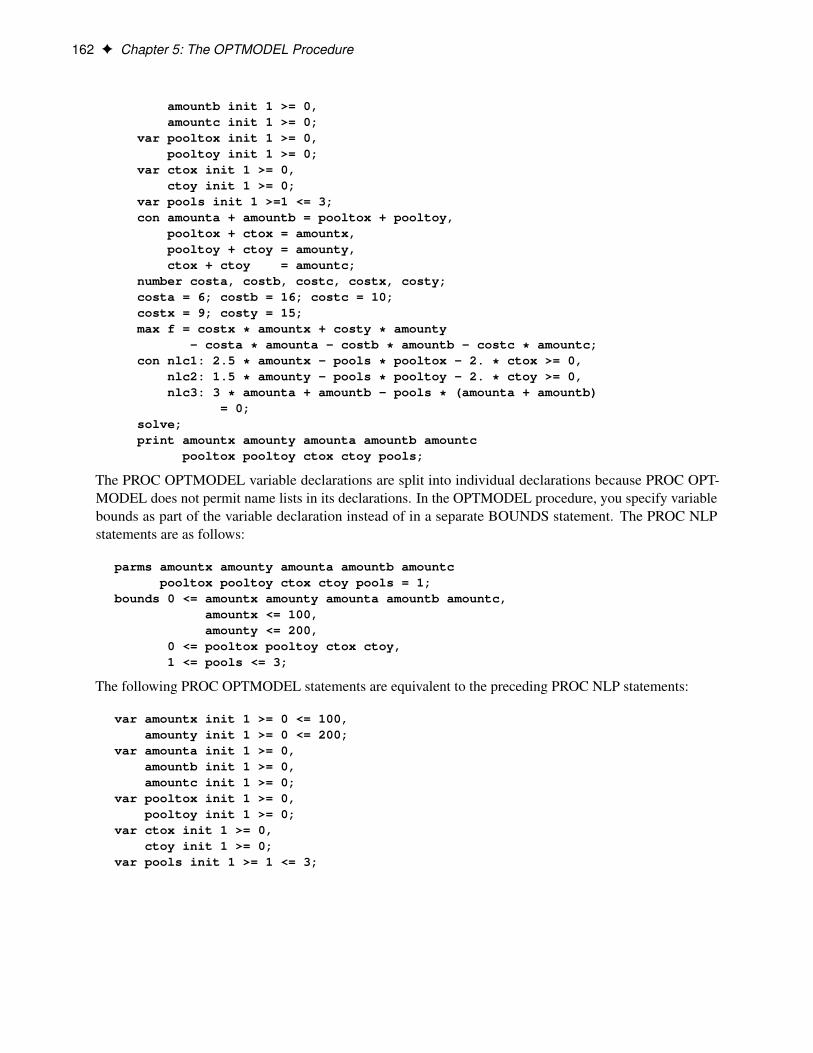
162 F Chapter 5: The OPTMODEL Procedure
amountb init 1 >= 0,amountc init 1 >= 0;
var pooltox init 1 >= 0,pooltoy init 1 >= 0;
var ctox init 1 >= 0,ctoy init 1 >= 0;
var pools init 1 >=1 <= 3;con amounta + amountb = pooltox + pooltoy,
pooltox + ctox = amountx,pooltoy + ctoy = amounty,ctox + ctoy = amountc;
number costa, costb, costc, costx, costy;costa = 6; costb = 16; costc = 10;costx = 9; costy = 15;max f = costx * amountx + costy * amounty
- costa * amounta - costb * amountb - costc * amountc;con nlc1: 2.5 * amountx - pools * pooltox - 2. * ctox >= 0,
nlc2: 1.5 * amounty - pools * pooltoy - 2. * ctoy >= 0,nlc3: 3 * amounta + amountb - pools * (amounta + amountb)
= 0;solve;print amountx amounty amounta amountb amountc
pooltox pooltoy ctox ctoy pools;
The PROC OPTMODEL variable declarations are split into individual declarations because PROC OPT-MODEL does not permit name lists in its declarations. In the OPTMODEL procedure, you specify variablebounds as part of the variable declaration instead of in a separate BOUNDS statement. The PROC NLPstatements are as follows:
parms amountx amounty amounta amountb amountcpooltox pooltoy ctox ctoy pools = 1;
bounds 0 <= amountx amounty amounta amountb amountc,amountx <= 100,amounty <= 200,
0 <= pooltox pooltoy ctox ctoy,1 <= pools <= 3;
The following PROC OPTMODEL statements are equivalent to the preceding PROC NLP statements:
var amountx init 1 >= 0 <= 100,amounty init 1 >= 0 <= 200;
var amounta init 1 >= 0,amountb init 1 >= 0,amountc init 1 >= 0;
var pooltox init 1 >= 0,pooltoy init 1 >= 0;
var ctox init 1 >= 0,ctoy init 1 >= 0;
var pools init 1 >= 1 <= 3;
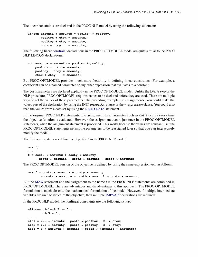
Rewriting PROC NLP Models for PROC OPTMODEL F 163
The linear constraints are declared in the PROC NLP model by using the following statement:
lincon amounta + amountb = pooltox + pooltoy,pooltox + ctox = amountx,pooltoy + ctoy = amounty,ctox + ctoy = amountc;
The following linear constraint declarations in the PROC OPTMODEL model are quite similar to the PROCNLP LINCON declarations:
con amounta + amountb = pooltox + pooltoy,pooltox + ctox = amountx,pooltoy + ctoy = amounty,ctox + ctoy = amountc;
But PROC OPTMODEL provides much more flexibility in defining linear constraints. For example, acoefficient can be a named parameter or any other expression that evaluates to a constant.
The cost parameters are declared explicitly in the PROC OPTMODEL model. Unlike the DATA step or theNLP procedure, PROC OPTMODEL requires names to be declared before they are used. There are multipleways to set the values of these parameters. The preceding example uses assignments. You could make thevalues part of the declaration by using the INIT expression clause or the = expression clause. You could alsoread the values from a data set by using the READ DATA statement.
In the original PROC NLP statements, the assignment to a parameter such as costa occurs every timethe objective function is evaluated. However, the assignment occurs just once in the PROC OPTMODELstatements, when the assignment statement is processed. This works because the values are constant. But thePROC OPTMODEL statements permit the parameters to be reassigned later so that you can interactivelymodify the model.
The following statements define the objective f in the PROC NLP model:
max f;. . .f = costx * amountx + costy * amounty
- costa * amounta - costb * amountb - costc * amountc;
The PROC OPTMODEL version of the objective is defined by using the same expression text, as follows:
max f = costx * amountx + costy * amounty- costa * amounta - costb * amountb - costc * amountc;
But the MAX statement and the assignment to the name f in the PROC NLP statements are combined inPROC OPTMODEL. There are advantages and disadvantages to this approach. The PROC OPTMODELformulation is much closer to the mathematical formulation of the model. However, if multiple intermediatevariables are used to structure the objective, then multiple IMPVAR declarations are required.
In the PROC NLP model, the nonlinear constraints use the following syntax:
nlincon nlc1-nlc2 >= 0.,nlc3 = 0.;
. . .nlc1 = 2.5 * amountx - pools * pooltox - 2. * ctox;nlc2 = 1.5 * amounty - pools * pooltoy - 2. * ctoy;nlc3 = 3 * amounta + amountb - pools * (amounta + amountb);

164 F Chapter 5: The OPTMODEL Procedure
In the PROC OPTMODEL model, the equivalent statements are as follows:
con nlc1: 2.5 * amountx - pools * pooltox - 2. * ctox >= 0,nlc2: 1.5 * amounty - pools * pooltoy - 2. * ctoy >= 0,nlc3: 3 * amounta + amountb - pools * (amounta + amountb)
= 0;
The nonlinear constraints in PROC OPTMODEL use the same syntax as linear constraints. In fact, if thevariable pools were declared as a parameter, then all the preceding constraints would be linear. The nonlinearconstraint in PROC OPTMODEL combines the NLINCON statement of PROC NLP with the assignment inthe PROC NLP statements. Objective names can be used in nonlinear constraint expressions to structure theformula as they are in objective expressions,
The PROC OPTMODEL model does not use a RUN statement to invoke the solver. Instead the solveris invoked interactively by the SOLVE statement in PROC OPTMODEL. By default, the OPTMODELprocedure prints much less information about the optimization process. Generally this information consists ofmessages from the solver (such as the termination reason) and a short status display. The PROC OPTMODELstatements add a PRINT statement in order to display the variable estimates from the solver.
Examples: OPTMODEL Procedure
Example 5.1: Matrix Square RootThis example demonstrates the use of PROC OPTMODEL array parameters and variables. The followingstatements create a randomized positive definite symmetric matrix and define an optimization model to findthe matrix square root of the generated matrix:
proc optmodel;number n = 5; /* size of matrix *//* random original array */number A{1..n, 1..n} = 10 - 20*rand('UNIFORM');/* compute upper triangle of the
* symmetric matrix A*transpose(A) *//* should be positive def unless A is singular */number P{i in 1..n, j in i..n};for {i in 1..n, j in i..n}
P[i,j] = sum{k in 1..n} A[i,k]*A[j,k];/* coefficients of square root array
* (upper triangle of symmetric matrix) */var q{i in 1..n, i..n};/* The default initial value q[i,j]=0 is
* a local minimum of the objective,
* so you must move it away from that point. */q[1,1] = 1;/* minimize difference of square of q from P */min r = sum{i in 1..n, j in i..n}
( sum{k in 1..i} q[k,i]*q[k,j]+ sum{k in i+1..j} q[i,k]*q[k,j]+ sum{k in j+1..n} q[i,k]*q[j,k]

Example 5.2: Reading From and Creating a Data Set F 165
- P[i,j] )**2;solve;print q;
These statements define a random array A of size n � n. The product P is defined as the matrix productAAT . The product is symmetric, so the declaration of the parameter P gives it upper triangular indexing. Thematrix represented by P should be positive definite unless A is singular. But singularity is unlikely becauseof the random generation of A. If P is positive definite, then it has a well-defined square root, Q, such thatP D QQT .
The objective r simply minimizes the sum of squares of the coefficients as
r DX
1�i�j�n
R2i;j
where R D QQT � P . (This technique for computing matrix square roots is intended only for thedemonstration of PROC OPTMODEL capabilities. Better methods exist.)
Output 5.1.1 shows part of the output from running these statements. The values that are actually displayeddepend on the random numbers generated.
Output 5.1.1 Matrix Square Root Results
q
1 2 3 4 5
1 -0.10557 -7.03961 8.64638 1.89284 -8.28542
2 5.23609 0.64462 -6.63339 6.71074
3 -1.61894 -7.31866 1.14428
4 3.76627 0.32063
5 4.93412
Example 5.2: Reading From and Creating a Data SetThis example demonstrates how to use the READ DATA statement to read parameters from a SAS data set.The objective is the Bard function, which is the following least squares problem with I D f1; 2; : : : ; 15g:
f .x/ D1
2
Xk2I
�yk �
�x1 C
k
vkx2 C wkx3
��2x D .x1; x2; x3/; y D .y1; y2; : : : ; y15/
where vk D 16 � k, wk D min.k; vk/ (k 2 I ), and
y D .0:14; 0:18; 0:22; 0:25; 0:29; 0:32; 0:35; 0:39; 0:37; 0:58; 0:73; 0:96; 1:34; 2:10; 4:39/
The minimum function value f .x�/ D 4.107E–3 is at the point .0:08; 1:13; 2:34/. The starting pointx0 D .1; 1; 1/ is used. This problem is identical to the example “Using the DATA= Option” in Chapter6, “The NLP Procedure” (SAS/OR User’s Guide: Mathematical Programming Legacy Procedures). Thefollowing statements use the READ DATA statement to input parameter values and the CREATE DATAstatement to save the solution in a SAS data set:

166 F Chapter 5: The OPTMODEL Procedure
data bard;input y @@;datalines;
.14 .18 .22 .25 .29 .32 .35 .39
.37 .58 .73 .96 1.34 2.10 4.39;proc optmodel;
set I = 1..15;number y{I};read data bard into [_n_] y;number v{k in I} = 16 - k;number w{k in I} = min(k, v[k]);var x{1..3} init 1;min f = 0.5*
sum{k in I}(y[k] - (x[1] + k /
(v[k]*x[2] + w[k]*x[3])))**2;solve;print x;create data xdata from [i] xd=x;
In these statements the values for parameter y are read from the BARD data set. The set I indexes the termsof the objective in addition to the y array.
The preceding statements define two utility parameters that contain coefficients used in the objective function.These coefficients could have been defined in the expression for the objective, f, but it was convenient to givethem names and simplify the objective expression.
The result is shown in Output 5.2.1.
Output 5.2.1 Bard Function Solution
[1] x
1 0.08241
2 1.13303
3 2.34370
The final CREATE DATA statement saves the solution values determined by the solver into the data setXDATA. The data set contains an observation for each x index. Each observation contains two variables. Theoutput variable i contains the index, while xd contains the value for the indexed entry in the array x. Theresulting data can be seen by using the PRINT procedure as follows:
proc print data=xdata;run;
The output from PROC PRINT is shown in Output 5.2.2.
Output 5.2.2 Output Data Set Contents
Obs i xd
1 1 0.08241
2 2 1.13303
3 3 2.34370

Example 5.3: Model Construction F 167
Example 5.3: Model ConstructionThis example uses PROC OPTMODEL features to simplify the construction of a mathematically formulatedmodel. The model is based on the example “An Assignment Problem” in Chapter 4, “The LP Procedure”(SAS/OR User’s Guide: Mathematical Programming Legacy Procedures). A single invocation of PROCOPTMODEL replaces several steps in the PROC LP statements.
The model assigns production of various grades of cloth to a set of machines in order to maximize profit whilemeeting customer demand. Each machine has different capacities to produce the various grades of cloth.(See the PROC LP example “An Assignment Problem” for more details.) The mathematical formulation,where xijk represents the amount of cloth of grade j to produce on machine k for customer i, follows:
maxPijk rijkxijk
subject toPk xijk D dij for all i and jPij cjkxijk � ak for all k
xijk � 0 for all i; j; and k
The OBJECT, DEMAND, and RESOURCE data sets are the same as in the PROC LP example. A new dataset, GRADE, is added to help separate the data from the model.
title 'An Assignment Problem';
data grade(drop=i);do i = 1 to 6;
grade = 'grade'||put(i,1.);output;
end;run;
data object;input machine customer
grade1 grade2 grade3 grade4 grade5 grade6;datalines;
1 1 102 140 105 105 125 1481 2 115 133 118 118 143 1661 3 70 108 83 83 88 861 4 79 117 87 87 107 1051 5 77 115 90 90 105 1482 1 123 150 125 124 154 .2 2 130 157 132 131 166 .2 3 103 130 115 114 129 .2 4 101 128 108 107 137 .2 5 118 145 130 129 154 .3 1 83 . . 97 122 1473 2 119 . . 133 163 1803 3 67 . . 91 101 1013 4 85 . . 104 129 1293 5 90 . . 114 134 1794 1 108 121 79 . 112 1324 2 121 132 92 . 130 150

168 F Chapter 5: The OPTMODEL Procedure
4 3 78 91 59 . 77 724 4 100 113 76 . 109 1044 5 96 109 77 . 105 145;
data demand;input customer
grade1 grade2 grade3 grade4 grade5 grade6;datalines;
1 100 100 150 150 175 2502 300 125 300 275 310 3253 400 0 400 500 340 04 250 0 750 750 0 05 0 600 300 0 210 360;
data resource;input machine
grade1 grade2 grade3 grade4 grade5 grade6 avail;datalines;
1 .250 .275 .300 .350 .310 .295 7442 .300 .300 .305 .315 .320 . 2443 .350 . . .320 .315 .300 7904 .280 .275 .260 . .250 .295 672;
The following PROC OPTMODEL statements read the data sets, build the linear programming model, solvethe model, and output the optimal solution to a SAS data set called SOLUTION:
proc optmodel;/* declare index sets */set CUSTOMERS;set <str> GRADES;set MACHINES;
/* declare parameters */num return {CUSTOMERS, GRADES, MACHINES} init 0;num demand {CUSTOMERS, GRADES};num cost {GRADES, MACHINES} init 0;num avail {MACHINES};
/* read the set of grades */read data grade into GRADES=[grade];
/* read the set of customers and their demands */read data demand
into CUSTOMERS=[customer]{j in GRADES} <demand[customer,j]=col(j)>;
/* read the set of machines, costs, and availability */read data resource nomiss
into MACHINES=[machine]{j in GRADES} <cost[j,machine]=col(j)>avail;

Example 5.3: Model Construction F 169
/* read objective data */read data object nomiss
into [machine customer]{j in GRADES} <return[customer,j,machine]=col(j)>;
/* declare the model */var AmountProduced {CUSTOMERS, GRADES, MACHINES} >= 0;max TotalReturn = sum {i in CUSTOMERS, j in GRADES, k in MACHINES}
return[i,j,k] * AmountProduced[i,j,k];con req_demand {i in CUSTOMERS, j in GRADES}:
sum {k in MACHINES} AmountProduced[i,j,k] = demand[i,j];con req_avail {k in MACHINES}:
sum {i in CUSTOMERS, j in GRADES}cost[j,k] * AmountProduced[i,j,k] <= avail[k];
/* call the solver and save the results */solve;create data solution
from [customer grade machine] = {i in CUSTOMERS, j in GRADES,k in MACHINES: AmountProduced[i,j,k].sol ne 0}
amount=AmountProduced;
/* print optimal solution */print AmountProduced;
quit;
The statements use both numeric (NUM) and character (STR) index sets, which are populated from thecorresponding data set variables in the READ DATA statements. The OPTMODEL parameters can be eithersingle-dimensional (AVAIL) or multiple-dimensional (COST, DEMAND, RETURN). The RETURN andCOST parameters are given initial values of 0, and the NOMISS option in the READ DATA statement tellsPROC OPTMODEL to read only the nonmissing values from the input data sets. The model declarationis nearly identical to the mathematical formulation. The logical condition AmountProduced[i,j,k].sol
ne 0 in the CREATE DATA statement ensures that only the nonzero parts of the solution appear in theSOLUTION data set. In the PROC LP example, the creation of this data set required postprocessing of thePROC LP output data set.
The solver produces the following problem summary and solution summary:

170 F Chapter 5: The OPTMODEL Procedure
Output 5.3.1 LP Solver Result
An Assignment ProblemAn Assignment Problem
Problem Summary
Objective Sense Maximization
Objective Function TotalReturn
Objective Type Linear
Number of Variables 120
Bounded Above 0
Bounded Below 120
Bounded Below and Above 0
Free 0
Fixed 0
Number of Constraints 34
Linear LE (<=) 4
Linear EQ (=) 30
Linear GE (>=) 0
Linear Range 0
Constraint Coefficients 220
Solution Summary
Solver LP
Algorithm Dual Simplex
Objective Function TotalReturn
Solution Status Optimal
Objective Value 871426.03763
Primal Infeasibility 0
Dual Infeasibility 0
Bound Infeasibility 0
Iterations 58
Presolve Time 0.00
Solution Time 0.00
The SOLUTION data set can be processed by PROC TABULATE as follows to create a compact representationof the solution:
proc tabulate data=solution;class customer grade machine;var amount;table (machine*customer), (grade*amount=''*sum='');
run;
These statements produce the table shown in Output 5.3.2.

Example 5.4: Set Manipulation F 171
Output 5.3.2 An Assignment Problem
An Assignment ProblemAn Assignment Problem
grade
grade1 grade2 grade3 grade4 grade5 grade6
machine customer
1 1 . 100.00 150.00 150.00 175.00 250.00
2 . . 300.00 . . .
3 . . 256.72 210.31 . .
4 . . 750.00 . . .
5 . 92.27 . . . .
2 3 . . 143.28 . 340.00 .
5 . . 300.00 . . .
3 2 . . . 275.00 310.00 325.00
3 . . . 289.69 . .
4 . . . 750.00 . .
5 . . . . 210.00 360.00
4 1 100.00 . . . . .
2 300.00 125.00 . . . .
3 400.00 . . . . .
4 250.00 . . . . .
5 . 507.73 . . . .
Example 5.4: Set ManipulationThis example demonstrates PROC OPTMODEL set manipulation operators. These operators are used tocompute the set of primes up to a given limit. This example does not solve an optimization problem, butsimilar set manipulation could be used to set up an optimization model. Here are the statements:
proc optmodel;number maxprime; /* largest number to consider */set composites =
union {i in 3..sqrt(maxprime) by 2} i*i..maxprime by 2*i;set primes = {2} union (3..maxprime by 2 diff composites);maxprime = 500;put primes;
The set composites contains the odd composite numbers up to the value of the parameter maxprime. The evennumbers are excluded here to reduce execution time and memory requirements. The UNION aggregationoperation is used in the definition to combine the sets of odd multiples of i for i D 3; 5; : : :. Any compositenumber less than the value of the parameter maxprime has a divisor �
pmaxprime, so the range of i can be
limited. The set of multiples of i can also be started at i � i since smaller multiples are found in the set ofmultiples for a smaller index.
You can then define the set primes. The odd primes are determined by using the DIFF operator to remove thecomposites from the set of odd numbers no greater than the parameter maxprime. The UNION operator addsthe single even prime, 2, to the resulting set of primes.
The PUT statement produces the result in Output 5.4.1.

172 F Chapter 5: The OPTMODEL Procedure
Output 5.4.1 Primes less than or equal to 500
{2,3,5,7,11,13,17,19,23,29,31,37,41,43,47,53,59,61,67,71,73,79,83,89,97,101,103,107,109,113,127,131,137,139,149,151,157,163,167,173,179,181,191,193,197,199,211,223,227,229,233,239,241,251,257,263,269,271,277,281,283,293,307,311,313,317,331,337,347,349,353,359,367,373,379,383,389,397,401,409,419,421,431,433,439,443,449,457,461,463,467,479,487,491,499}
Note that you were able to delay the definition of the value of the parameter maxprime until just before thePUT statement. Since the defining expressions of the SET declarations are handled symbolically, the valueof maxprime is not necessary until you need the value of the set primes. Because the sets composites andprimes are defined symbolically, their values reflect any changes to the parameter maxprime. You can seethis update by appending the following statements to the preceding statements:
maxprime = 50;put primes;
The additional statements produce the results in Output 5.4.2. The value of the set primes has been recomputedto reflect the change to the parameter maxprime.
Output 5.4.2 Primes less than or equal to 50
{2,3,5,7,11,13,17,19,23,29,31,37,41,43,47}
Example 5.5: Multiple SubproblemsMany important optimization problems cannot be solved directly using a standard solver, either because theproblem has constraints that cannot be modeled directly or because the resulting model would be too large tobe practical. For these types of problems, you can use PROC OPTMODEL to synthesize solution methodsby using a combination of the existing solvers and the modeling language programming constructions. Thisexample demonstrates the use of multiple subproblems to solve the cutting stock problem.
The cutting stock problem determines how to efficiently cut raw stock into finished widths based on thedemands for the final product. Consider the example from page 195 of Chvátal (1983), where raw stock hasa width of 100 inches and the demands are shown in Table 5.18.
Table 5.18 Cutting Stock Demand
Finished Width Demand45 inches 9735 inches 61031 inches 39514 inches 211
A portion of the demand can be satisfied using a cutting pattern. For example, with the demands in Table 5.18a possible pattern cuts one final of width 35 inches, one final of width 31 inches, and two finals of width 14inches. This gives:
100 D 0 � 45C 1 � 35C 1 � 31C 2 � 14C waste:

Example 5.5: Multiple Subproblems F 173
The cutting stock problem can be formulated as follows, where xj represents the number of times pattern jappears, aij represents the number of times demand item i appears in pattern j, di is the demand for item i,wi is the width of item i, N represents the set of patterns, M represents the set of items, and W is the width ofthe raw stock:
minimizePj2N xj
subject toPj2N aijxj � di for all i 2M
xj integer; � 0 for all j 2 N
Also for each feasible pattern j you must have:Xi2M
wiaij � W
The difficulty with this formulation is that the number of patterns can be very large, with too many columnsxj to solve efficiently. But you can use column generation, as described on page 198 of Chvátal (1983), togenerate a smaller set of useful patterns, starting from an initial feasible set.
The dual variables, �i , of the demand constraints are used to price out the columns. From linear programming(LP) duality theory, a column that improves the primal solution must have a negative reduced cost. For thisproblem the reduced cost for column xj is
1 �Xi2M
�iaij
Using this observation produces a knapsack subproblem:
minimize 1 �Pi2M �iai
subject toPi2M wiai � W
ai integer; � 0 for all j 2 N
where the objective is equivalent to:
maximizePi2M �iai
The pattern is useful if the associated reduced cost is negative:
1 �Xi2M
�ia�i < 0
So you can use the following steps to generate the patterns and solve the cutting stock problem:
1. Initialize a set of trivial (one item) patterns.
2. Solve the problem using the LP solver.
3. Minimize the reduced cost using a knapsack solver.

174 F Chapter 5: The OPTMODEL Procedure
4. Include the new pattern if the reduced cost is negative.
5. Repeat steps 2 through 4 until there are no more negative reduced cost patterns.
These steps are implemented in the following statements. Since adding columns preserves primal feasibility,the statements use the primal simplex solver to take advantage of a warm start. The statements also solve theLP relaxation of the problem, but you want the integer solution. So the statements finish by using the MILPsolver with the integer restriction applied. The result is not guaranteed to be optimal, but lower and upperbounds can be provided for the optimal objective.
/* cutting-stock problem *//* uses delayed column generation from
Chvatal's Linear Programming (1983), page 198 */
%macro csp(capacity);proc optmodel printlevel=0;
/* declare parameters and sets */num capacity = &capacity;set ITEMS;num demand {ITEMS};num width {ITEMS};num num_patterns init card(ITEMS);set PATTERNS = 1..num_patterns;num a {ITEMS, PATTERNS};num c {ITEMS} init 0;num epsilon = 1E-6;
/* read input data */read data indata into ITEMS=[_N_] demand width;
/* generate trivial initial columns */for {i in ITEMS, j in PATTERNS}
a[i,j] = (if (i = j) then floor(capacity/width[i]) else 0);
/* define master problem */var x {PATTERNS} >= 0 integer;minimize NumberOfRaws = sum {j in PATTERNS} x[j];con demand_con {i in ITEMS}:
sum {j in PATTERNS} a[i,j] * x[j] >= demand[i];problem Master include x NumberOfRaws demand_con;
/* define column generation subproblem */var y {ITEMS} >= 0 integer;maximize KnapsackObjective = sum {i in ITEMS} c[i] * y[i];con knapsack_con:
sum {i in ITEMS} width[i] * y[i] <= capacity;problem Knapsack include y KnapsackObjective knapsack_con;
/* main loop */do while (1);
print _page_ a;
/* master problem */
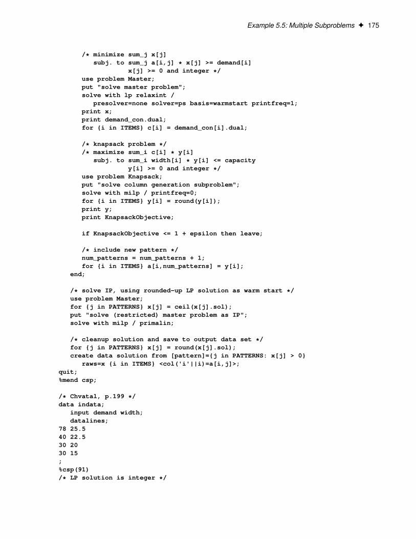
Example 5.5: Multiple Subproblems F 175
/* minimize sum_j x[j]subj. to sum_j a[i,j] * x[j] >= demand[i]
x[j] >= 0 and integer */use problem Master;put "solve master problem";solve with lp relaxint /
presolver=none solver=ps basis=warmstart printfreq=1;print x;print demand_con.dual;for {i in ITEMS} c[i] = demand_con[i].dual;
/* knapsack problem *//* maximize sum_i c[i] * y[i]
subj. to sum_i width[i] * y[i] <= capacityy[i] >= 0 and integer */
use problem Knapsack;put "solve column generation subproblem";solve with milp / printfreq=0;for {i in ITEMS} y[i] = round(y[i]);print y;print KnapsackObjective;
if KnapsackObjective <= 1 + epsilon then leave;
/* include new pattern */num_patterns = num_patterns + 1;for {i in ITEMS} a[i,num_patterns] = y[i];
end;
/* solve IP, using rounded-up LP solution as warm start */use problem Master;for {j in PATTERNS} x[j] = ceil(x[j].sol);put "solve (restricted) master problem as IP";solve with milp / primalin;
/* cleanup solution and save to output data set */for {j in PATTERNS} x[j] = round(x[j].sol);create data solution from [pattern]={j in PATTERNS: x[j] > 0}
raws=x {i in ITEMS} <col('i'||i)=a[i,j]>;quit;%mend csp;
/* Chvatal, p.199 */data indata;
input demand width;datalines;
78 25.540 22.530 2030 15;%csp(91)/* LP solution is integer */

176 F Chapter 5: The OPTMODEL Procedure
/* Chvatal, p.195 */data indata;
input demand width;datalines;
97 45610 36395 31211 14;%csp(100)/* LP solution is fractional */
The contents of the output data set for the second problem instance are shown in Output 5.5.1.
Output 5.5.1 Cutting Stock Solution
Obs pattern raws i1 i2 i3 i4
1 1 49 2 0 0 0
2 5 206 0 2 0 2
3 6 198 0 1 2 0
Example 5.6: Traveling Salesman ProblemThis example demonstrates the use of the SUBMIT statement to execute a block of SAS statements fromwithin a PROC OPTMODEL session. In this case, the SUBMIT block calls the GPLOT procedure todisplay intermediate results during the solution of an instance of the traveling salesman problem (TSP). Theproblem is described in Example 8.4. For an example of how to use PROC OPTNET to solve the TSP,see “Traveling Salesman Problem Applied to a Simple Directed Graph” (Chapter 2, SAS/OR User’s Guide:Network Optimization Algorithms).
The following DATA step converts a TSPLIB instance of type EUC_2D into a SAS data set that contains thecoordinates of the vertices:
/* convert the TSPLIB instance into a data set */data tspData(drop=H);
infile "&tsplib";input H $1. @;if H not in ('N','T','C','D','E');input @1 var1-var3;
run;
The following macro generates plots of the solution and objective value:
%macro plotTSP;/* create Annotate data set to draw subtours */data anno;
retain drawspace 'datavalue' linethickness 1 function 'line';set solData;
run;
title1 h=2 "TSP: Iter = &i, Objective = &&obj&i";title2;

Example 5.6: Traveling Salesman Problem F 177
proc sgplot data=tspData sganno=anno;scatter x=var2 y=var3 / datalabel=var1;xaxis display=none;yaxis display=none;
run;%mend plotTSP;
The following PROC OPTMODEL statements solve the TSP by using the subtour formulation and iterativelyadding subtour constraints. The SUBMIT statement calls the %plotTSP macro to plot the solution andobjective value at each stage.
/* iterative solution using the subtour formulation */proc optmodel;
set VERTICES;set EDGES = {i in VERTICES, j in VERTICES: i > j};num xc {VERTICES};num yc {VERTICES};
num numsubtour init 0;set SUBTOUR {1..numsubtour};
/* read in the instance and customer coordinates (xc, yc) */read data tspData into VERTICES=[var1] xc=var2 yc=var3;
/* the cost is the euclidean distance rounded to the nearest integer */num c {<i,j> in EDGES}
init floor( sqrt( ((xc[i]-xc[j])**2 + (yc[i]-yc[j])**2)) + 0.5);
var x {EDGES} binary;
/* minimize the total cost */min obj =
sum {<i,j> in EDGES} c[i,j] * x[i,j];
/* each vertex has exactly one in-edge and one out-edge */con two_match {i in VERTICES}:
sum {j in VERTICES: i > j} x[i,j]+ sum {j in VERTICES: i < j} x[j,i] = 2;
/* no subtours (these constraints are generated dynamically) */con subtour_elim {s in 1..numsubtour}:
sum {<i,j> in EDGES: (i in SUBTOUR[s] and j not in SUBTOUR[s])or (i not in SUBTOUR[s] and j in SUBTOUR[s])} x[i,j] >= 2;
/* this starts the algorithm to find violated subtours */set <num,num> EDGES1;set VERTICES1 = union{<i,j> in EDGES1} {i, j};num component {VERTICES1};num numcomp init 2;num iter init 1;call symput('i',trim(left(put(round(iter),best.))));num numiters init 1;

178 F Chapter 5: The OPTMODEL Procedure
/* initial solve with just matching constraints */solve;call symput(compress('obj'||put(iter,best.)),
trim(left(put(round(obj),best.))));
/* create a data set for use by PROC SGPLOT */create data solData from
[i j]={<i,j> in EDGES: x[i,j].sol > 0.5}x1=xc[i] y1=yc[i] x2=xc[j] y2=yc[j];
submit;%plotTSP;
endsubmit;/* while the solution is disconnected, continue */do while (numcomp > 1);
iter = iter + 1;call symput('i',trim(left(put(round(iter),best.))));
/* find connected components of support graph */EDGES1 = {<i,j> in EDGES: round(x[i,j].sol) = 1};solve with network /
links = (include=EDGES1)nodes = (include=VERTICES1)concompout = (concomp=component);
numcomp = _oroptmodel_num_["NUM_COMPONENTS"];if numcomp = 1 then leave;
numiters = iter;numsubtour = numsubtour + numcomp;for {comp in 1..numcomp} do;
SUBTOUR[numsubtour-numcomp+comp]= {i in VERTICES: component[i] = comp};
end;
solve;call symput(compress('obj'||put(iter,best.)),
trim(left(put(round(obj),best.))));
/* create a data set for use by PROC SGPLOT */create data solData from
[i j]={<i,j> in EDGES: x[i,j].sol > 0.5}x1=xc[i] y1=yc[i] x2=xc[j] y2=yc[j];
call symput('numiters',put(numiters,best.));submit;
%plotTSP;endsubmit;
end;quit;
The plot in Output 5.6.1 shows the solution and objective value at each stage. Each stage restricts somesubset of subtours. When you reach the final stage, you have a valid tour.

Example 5.6: Traveling Salesman Problem F 179
Output 5.6.1 Iterative Solution of Traveling Salesman Problem

180 F Chapter 5: The OPTMODEL Procedure
Output 5.6.1 continued
Example 5.7: Sparse ModelingThis example demonstrates how to rewrite certain models for more efficient processing. Sometimes optimiza-tion models that run out of memory during problem generation can be rewritten to take advantage of sparsityto use memory more efficiently. This often occurs when a large array is modeled in a dense format but mostof its entries are zeros. Usually, the array provides problem coefficients or it contains optimization variables.
The model for this example solves the facility location problem that is described in Example 8.3. Thisexample is concerned with the resources that are required for PROC OPTMODEL problem generation andsolver initialization. So the size of the problem has been increased, but the model has also been modified tomake it easier to solve. In order to handle the larger problem size, the model eliminates a large number of thepotential assignments of customers to facilities based on distance, making the problem sparse.
The following code generates a random instance of the facility location problem:
%let NumCustomers = 1500;%let NumSites = 250;%let SiteCapacity = 50;%let MaxDemand = 10;%let xmax = 200;%let ymax = 100;%let seed = 938;
/* generate random customer locations */data cdata(drop=i);
length name $8;call streaminit(&seed);do i = 1 to &NumCustomers;
name = compress('C'||put(i,best.));x = rand('UNIFORM') * &xmax;y = rand('UNIFORM') * &ymax;demand = 1;output;

Example 5.7: Sparse Modeling F 181
end;run;
/* generate random site locations and fixed charge */data sdata(drop=i);
length name $8;call streaminit(&seed);do i = 1 to &NumSites;
name = compress('SITE'||put(i,best.));x = rand('UNIFORM') * &xmax;y = rand('UNIFORM') * &ymax;fixed_charge = 300 * (abs(&xmax/2-x)/&xmax + abs(&ymax/2-y)/&ymax);output;
end;run;
The following code uses a dense version of the facility location model. This model is equivalent to the modelfrom Example 8.3 except for the added constraint distance_at_most_30. This constraint eliminates fromconsideration the assignment of customers to facilities over long distances by forcing the correspondingAssign variables to 0.
proc optmodel;performance details;profile on percent=0.1;set <str> CUSTOMERS;set <str> SITES init {};
/* x and y coordinates of CUSTOMERS and SITES */num x {CUSTOMERS union SITES};num y {CUSTOMERS union SITES};num demand {CUSTOMERS};num fixed_charge {SITES};
/* distance from customer i to site j */num dist {i in CUSTOMERS, j in SITES}
= sqrt((x[i] - x[j])^2 + (y[i] - y[j])^2);
read data cdata into CUSTOMERS=[name] x y demand;read data sdata into SITES=[name] x y fixed_charge;
var Assign {CUSTOMERS, SITES} binary;var Build {SITES} binary;
min CostNoFixedCharge= sum {i in CUSTOMERS, j in SITES} dist[i,j] * Assign[i,j];
min CostFixedCharge= CostNoFixedCharge + sum {j in SITES} fixed_charge[j] * Build[j];
/* each customer assigned to exactly one site */con assign_def {i in CUSTOMERS}:
sum {j in SITES} Assign[i,j] = 1;
/* if customer i assigned to site j, then facility must be built at j */con link {i in CUSTOMERS, j in SITES}:
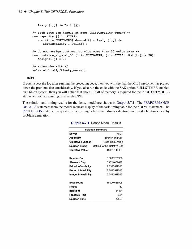
182 F Chapter 5: The OPTMODEL Procedure
Assign[i,j] <= Build[j];
/* each site can handle at most &SiteCapacity demand */con capacity {j in SITES}:
sum {i in CUSTOMERS} demand[i] * Assign[i,j] <=&SiteCapacity * Build[j];
/* do not assign customer to site more than 30 units away */con distance_at_most_30 {i in CUSTOMERS, j in SITES: dist[i,j] > 30}:
Assign[i,j] = 0;
/* solve the MILP */solve with milp/timetype=real;
quit;
If you inspect the log after running the preceding code, then you will see that the MILP presolver has pruneddown the problem size considerably. If you also run the code with the SAS option FULLSTIMER enabledon a 64-bit system, then you will notice that about 1.3GB of memory is required for the PROC OPTMODELstep when you are running on a single CPU.
The solution and timing results for the dense model are shown in Output 5.7.1. The PERFORMANCEDETAILS statement from the model requests display of the task timing table for the SOLVE statement. ThePROFILE ON statement requests further timing details, including evaluation time for declarations used byproblem generation.
Output 5.7.1 Dense Model Results
Solution Summary
Solver MILP
Algorithm Branch and Cut
Objective Function CostFixedCharge
Solution Status Optimal within Relative Gap
Objective Value 18001.140353
Relative Gap 0.0000261906
Absolute Gap 0.4714482429
Primal Infeasibility 2.839542E-13
Bound Infeasibility 2.787291E-13
Integer Infeasibility 2.787291E-13
Best Bound 18000.668905
Nodes 13
Iterations 34484
Presolve Time 0.84
Solution Time 54.59

Example 5.7: Sparse Modeling F 183
Output 5.7.1 continued
Procedure Task Timing
TaskTime
(sec.) Time
Problem Generation 4.06 6.77%
Solver Initialization 0.66 1.10%
Code Generation 0.03 0.05%
Presolve 0.84 1.40%
Root Node Processing 45.24 75.45%
Branch And Cut 6.48 10.81%
Synchronization 0.13 0.22%
Idle 1.85 3.09%
Other Tasks 0.04 0.07%
Solver Postprocessing 0.63 1.05%
Profile Information
Item Line Col.Execution
CountNet Time
(sec.)Wait Time
(sec.)% Total
Time
SOLVE 3558 4 1 56.33 2.11 84.9%
Constraint distance_at_most_30 3554 8 5.59 0.00 8.4%
Constraint link 3545 8 3.02 0.00 4.6%
Min CostNoFixedCharge 3535 8 0.31 0.00 0.5%
Number dist 3526 8 0.31 0.00 0.5%
Constraint capacity 3549 8 0.29 0.00 0.4%
Var Assign 3532 8 0.25 0.00 0.4%
Constraint assign_def 3541 8 0.23 0.00 0.3%
Other profiled items 0.00 0.00 0.0%
Note: Total profiled time is 66.34 seconds.
The best approach for reducing the memory requirements is to eliminate the Assign variables that are alwaysgoing to be 0. This is accomplished in the following sparse version of the code. Instead of indexing Assignover the crossproduct of CUSTOMERS and SITES, now the code defines a new set of pairs that satisfy thedistance requirement, CUSTOMERS_SITES. This set replaces the constraint distance_at_most_30 in thedense model. The objective and constraints have been modified to use the new indexing scheme, with implicitset slicing (as described in the section “More on Index Sets” on page 157) for constraints assign_def andcapacity.
proc optmodel;performance details;profile on percent=0.1;set <str> CUSTOMERS;set <str> SITES init {};
/* x and y coordinates of CUSTOMERS and SITES */num x {CUSTOMERS union SITES};num y {CUSTOMERS union SITES};num demand {CUSTOMERS};num fixed_charge {SITES};
/* distance from customer i to site j */

184 F Chapter 5: The OPTMODEL Procedure
num dist {i in CUSTOMERS, j in SITES}= sqrt((x[i] - x[j])^2 + (y[i] - y[j])^2);
read data cdata into CUSTOMERS=[name] x y demand;read data sdata into SITES=[name] x y fixed_charge;
set CUSTOMERS_SITES = {i in CUSTOMERS, j in SITES: dist[i,j] <= 30};var Assign {CUSTOMERS_SITES} binary;var Build {SITES} binary;
min CostNoFixedCharge= sum {<i,j> in CUSTOMERS_SITES} dist[i,j] * Assign[i,j];
min CostFixedCharge= CostNoFixedCharge + sum {j in SITES} fixed_charge[j] * Build[j];
/* each customer assigned to exactly one site */con assign_def {i in CUSTOMERS}:
sum {<(i),j> in CUSTOMERS_SITES} Assign[i,j] = 1;
/* if customer i assigned to site j, then facility must be built at j */con link {<i,j> in CUSTOMERS_SITES}:
Assign[i,j] <= Build[j];
/* each site can handle at most &SiteCapacity demand */con capacity {j in SITES}:
sum {<i,(j)> in CUSTOMERS_SITES} demand[i] * Assign[i,j] <=&SiteCapacity * Build[j];
/* solve the MILP */solve with milp/timetype=real;
quit;
The log from running the preceding code shows that the MILP presolver does not find anything to improvewith this version of the model. On a 64-bit system, the FULLSTIMER option shows that memory requirementshave been reduced to about 580MB when you are running on a single CPU, less than half the requirements ofthe previous model.
The solution and timing results for the dense model are shown in Output 5.7.2. Note that the dense model(Output 5.7.1) and the sparse model (Output 5.7.2) are equivalent after presolver processing and generate thesame result using similar amounts of solver time. On the other hand, problem generation time is significantlyreduced as are other times including presolve time. Both models used the solver option TIMETYPE=REALso that all times are reported in seconds of real time. You can see from the “Profile Information” table thatthe overhead associated with problem declarations has been significantly reduced.

Example 5.7: Sparse Modeling F 185
Output 5.7.2 Sparse Model Results
Solution Summary
Solver MILP
Algorithm Branch and Cut
Objective Function CostFixedCharge
Solution Status Optimal within Relative Gap
Objective Value 18001.140353
Relative Gap 0.0000261906
Absolute Gap 0.4714482429
Primal Infeasibility 2.839542E-13
Bound Infeasibility 2.787291E-13
Integer Infeasibility 2.787291E-13
Best Bound 18000.668905
Nodes 13
Iterations 34484
Presolve Time 2.70
Solution Time 56.53
Procedure Task Timing
TaskTime
(sec.) Time
Problem Generation 0.88 1.53%
Solver Initialization 0.09 0.15%
Code Generation 0.00 0.00%
Presolve 2.70 4.70%
Root Node Processing 45.33 78.78%
Branch And Cut 6.48 11.26%
Synchronization 0.12 0.22%
Idle 1.86 3.23%
Other Tasks 0.04 0.07%
Solver Postprocessing 0.03 0.05%
Profile Information
Item Line Col.Execution
CountNet Time
(sec.)Wait Time
(sec.)% Total
Time
SOLVE 3608 4 1 56.69 0.13 97.9%
Constraint link 3599 8 0.39 0.00 0.7%
Set CUSTOMERS_SITES 3585 8 0.36 0.00 0.6%
Number dist 3579 8 0.30 0.00 0.5%
Constraint assign_def 3595 8 0.07 0.00 0.1%
Other profiled items 0.12 0.00 0.2%
Note: Total profiled time is 57.94 seconds.
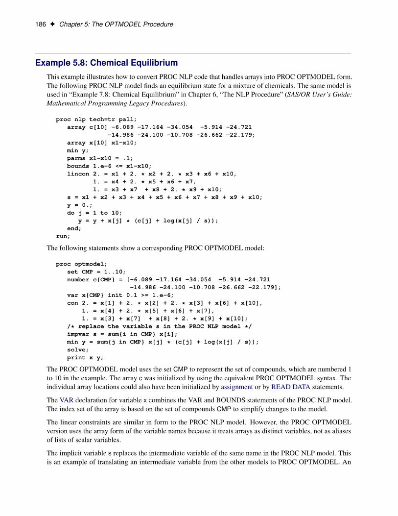
186 F Chapter 5: The OPTMODEL Procedure
Example 5.8: Chemical EquilibriumThis example illustrates how to convert PROC NLP code that handles arrays into PROC OPTMODEL form.The following PROC NLP model finds an equilibrium state for a mixture of chemicals. The same model isused in “Example 7.8: Chemical Equilibrium” in Chapter 6, “The NLP Procedure” (SAS/OR User’s Guide:Mathematical Programming Legacy Procedures).
proc nlp tech=tr pall;array c[10] -6.089 -17.164 -34.054 -5.914 -24.721
-14.986 -24.100 -10.708 -26.662 -22.179;array x[10] x1-x10;min y;parms x1-x10 = .1;bounds 1.e-6 <= x1-x10;lincon 2. = x1 + 2. * x2 + 2. * x3 + x6 + x10,
1. = x4 + 2. * x5 + x6 + x7,1. = x3 + x7 + x8 + 2. * x9 + x10;
s = x1 + x2 + x3 + x4 + x5 + x6 + x7 + x8 + x9 + x10;y = 0.;do j = 1 to 10;
y = y + x[j] * (c[j] + log(x[j] / s));end;
run;
The following statements show a corresponding PROC OPTMODEL model:
proc optmodel;set CMP = 1..10;number c{CMP} = [-6.089 -17.164 -34.054 -5.914 -24.721
-14.986 -24.100 -10.708 -26.662 -22.179];var x{CMP} init 0.1 >= 1.e-6;con 2. = x[1] + 2. * x[2] + 2. * x[3] + x[6] + x[10],
1. = x[4] + 2. * x[5] + x[6] + x[7],1. = x[3] + x[7] + x[8] + 2. * x[9] + x[10];
/* replace the variable s in the PROC NLP model */impvar s = sum{i in CMP} x[i];min y = sum{j in CMP} x[j] * (c[j] + log(x[j] / s));solve;print x y;
The PROC OPTMODEL model uses the set CMP to represent the set of compounds, which are numbered 1to 10 in the example. The array c was initialized by using the equivalent PROC OPTMODEL syntax. Theindividual array locations could also have been initialized by assignment or by READ DATA statements.
The VAR declaration for variable x combines the VAR and BOUNDS statements of the PROC NLP model.The index set of the array is based on the set of compounds CMP to simplify changes to the model.
The linear constraints are similar in form to the PROC NLP model. However, the PROC OPTMODELversion uses the array form of the variable names because it treats arrays as distinct variables, not as aliasesof lists of scalar variables.
The implicit variable s replaces the intermediate variable of the same name in the PROC NLP model. Thisis an example of translating an intermediate variable from the other models to PROC OPTMODEL. An

Example 5.8: Chemical Equilibrium F 187
alternative way is to use an additional constraint for every intermediate variable. Instead of declaring objectives as in the preceding statements, you can use the following statements:
. . .var s;con s = sum{i in CMP} x[i];. . .
Note that this alternative formulation passes an extra variable and constraint to the solver. This formulationcan sometimes be solved more efficiently, depending on the characteristics of the model.
The PROC OPTMODEL version uses a SUM operator over the set CMP, which enhances the flexibility ofthe model to accommodate possible changes in the set of compounds.
In the PROC NLP model, the objective function y is determined by an explicit loop. The DO loop in PROCNLP is replaced by a SUM aggregation operation in PROC OPTMODEL. The accumulation in the PROCNLP model is now performed by PROC OPTMODEL by using the SUM operator.
This PROC OPTMODEL model can be generalized further. Note that the array initialization and constraintsassume a fixed set of compounds. You can rewrite the model to handle an arbitrary number of compoundsand chemical elements. The new model loads the linear constraint coefficients from a data set along with theobjective coefficients for the parameter c, as follows:
data comp;input c a_1 a_2 a_3;datalines;
-6.089 1 0 0-17.164 2 0 0-34.054 2 0 1-5.914 0 1 0-24.721 0 2 0-14.986 1 1 0-24.100 0 1 1-10.708 0 0 1-26.662 0 0 2-22.179 1 0 1;
data atom;input b @@;datalines;
2. 1. 1.;
proc optmodel;set CMP;set ELT;number c{CMP};number a{ELT,CMP};number b{ELT};read data atom into ELT=[_n_] b;read data comp into CMP=[_n_]
c {i in ELT} < a[i,_n_]=col("a_"||i) >;var x{CMP} init 0.1 >= 1.e-6;

188 F Chapter 5: The OPTMODEL Procedure
con bal{i in ELT}: b[i] = sum{j in CMP} a[i,j]*x[j];impvar s = sum{i in CMP} x[i];min y = sum{j in CMP} x[j] * (c[j] + log(x[j] / s));print a b;solve;print x;
This version adds coefficients for the linear constraints to the COMP data set. The data set variable a_nrepresents the number of atoms in the compound for element n. The READ DATA statement for COMP usesthe iterated column syntax to read each of the data set variables a_n into the appropriate location in the arraya. In this example the expanded data set variable names are a_1, a_2, and a_3.
The preceding version also adds a new set, ELT, of chemical elements and a numeric parameter, b, thatrepresents the left-hand side of the linear constraints. The data values for the parameters ELT and b are readfrom the data set ATOM. The model can handle varying sets of chemical elements because of this extra dataset and the new parameters.
The linear constraints have been converted to a single, indexed family of constraints. One constraint is appliedfor each chemical element in the set ELT. The constraint expression uses a simple form that applies generallyto linear constraints. The following PRINT statement in the model shows the values that are read from thedata sets to define the linear constraints:
print a b;
The PRINT statements in the model produce the results shown in Output 5.8.1.
Output 5.8.1 PROC OPTMODEL Output
a
1 2 3 4 5 6 7 8 9 10
1 1 2 2 0 0 1 0 0 0 1
2 0 0 0 1 2 1 1 0 0 0
3 0 0 1 0 0 0 1 1 2 1
[1] b
1 2
2 1
3 1
[1] x
1 0.04066848
2 0.14773067
3 0.78315260
4 0.00141459
5 0.48524616
6 0.00069358
7 0.02739955
8 0.01794757
9 0.03731444
10 0.09687143

Example 5.8: Chemical Equilibrium F 189
In the preceding model, the chemical elements and compounds are designated by numbers. So in the PRINToutput, for example, the row that is labeled “3” represents the amount of the compound H2O. PROCOPTMODEL is capable of using more symbolic strings to designate array indices. The following version ofthe model uses strings to index arrays:
data comp;input name $ c a_h a_n a_o;datalines;
H -6.089 1 0 0H2 -17.164 2 0 0H2O -34.054 2 0 1N -5.914 0 1 0N2 -24.721 0 2 0NH -14.986 1 1 0NO -24.100 0 1 1O -10.708 0 0 1O2 -26.662 0 0 2OH -22.179 1 0 1;data atom;
input name $ b;datalines;
H 2.N 1.O 1.;proc optmodel;
set<string> CMP;set<string> ELT;number c{CMP};number a{ELT,CMP};number b{ELT};read data atom into ELT=[name] b;read data comp into CMP=[name]
c {i in ELT} < a[i,name]=col("a_"||i) >;var x{CMP} init 0.1 >= 1.e-6;con bal{i in ELT}: b[i] = sum{j in CMP} a[i,j]*x[j];impvar s = sum{i in CMP} x[i];min y = sum{j in CMP} x[j] * (c[j] + log(x[j] / s));solve;print x;
In this model, the sets CMP and ELT are now sets of strings. The data sets provide the names of the compoundsand elements. The names of the data set variables for atom counts in the data set COMP now include thechemical element symbol as part of their spelling. For example, the atom count for element H (hydrogen)is named a_h. Note that these changes did not require any modification to the specifications of the linearconstraints or of the objective.
The PRINT statement in the preceding statements produces the results shown in Output 5.8.2. The indices ofvariable x are now strings that represent the actual compounds.

190 F Chapter 5: The OPTMODEL Procedure
Output 5.8.2 PROC OPTMODEL Output with Strings
[1] x
H 0.04066848
H2 0.14773067
H2O 0.78315260
N 0.00141459
N2 0.48524616
NH 0.00069358
NO 0.02739955
O 0.01794757
O2 0.03731444
OH 0.09687143
References
Abramowitz, M., and Stegun, I. A., eds. (1972). Handbook of Mathematical Functions with Formulas,Graphs, and Mathematical Tables. 10th printing. New York: Dover.
Bazaraa, M. S., Sherali, H. D., and Shetty, C. M. (1993). Nonlinear Programming: Theory and Algorithms.New York: John Wiley & Sons.
Chvátal, V. (1983). Linear Programming. New York: W. H. Freeman.
Dennis, J. E., and Schnabel, R. B. (1983). Numerical Methods for Unconstrained Optimization and NonlinearEquations. Englewood Cliffs, NJ: Prentice-Hall.
Fletcher, R. (1987). Practical Methods of Optimization. 2nd ed. Chichester, UK: John Wiley & Sons.
Nocedal, J., and Wright, S. J. (1999). Numerical Optimization. New York: Springer-Verlag.

Subject Index
aggregation operatorsOPTMODEL procedure, 94
Bard function, 165
CLOSEFILE statementOPTMODEL procedure, 120
columns, 115complementarity
OPTMODEL procedure, 113constraint bodies
OPTMODEL procedure, 130constraint declaration
OPTMODEL procedure, 42constraints
OPTMODEL procedure, 28, 127control flow
OPTMODEL procedure, 119conversions
OPTMODEL procedure, 153
data set input/outputOPTMODEL procedure, 115
declaration statementsOPTMODEL procedure, 42
dual valueOPTMODEL procedure, 136
expressionsOPTMODEL procedure, 98
FCMP routinesOPTMODEL procedure, 154
feasible region, 113OPTMODEL procedure, 28
feasible solution, 113OPTMODEL procedure, 28
FILE statementOPTMODEL procedure, 120
first-order necessary conditionslocal minimum, 114
FOR statementOPTMODEL procedure, 119
formatted outputOPTMODEL procedure, 119
function expressionsOPTMODEL procedure, 101
functional summaryOPTMODEL procedure, 36
global solution, 113
identifier expressionsOPTMODEL procedure, 100
IF expression, 104impure functions
OPTMODEL procedure, 95index sets, 94
implicit set slicing, 158index-set-item, 102OPTMODEL procedure, 102
integer variablesOPTMODEL procedure, 135
intermediate variable, 186
Karush-Kuhn-Tucker conditions, 114key columns, 115, 117key set, 62
Lagrange multipliers, 114Lagrangian function, 114linear programming
OPTMODEL procedure, 28list form
PRINT statement, 75local minimum
first-order necessary conditions, 114second-order necessary conditions, 114
local solution, 113
macro variable_OROPTMODEL_, 159
matrix formPRINT statement, 76
migration to PROC OPTMODELfrom PROC NLP, 161
model updateOPTMODEL procedure, 143
MPS format, 85multiple solutions
OPTMODEL procedure, 149multiple subproblems
OPTMODEL procedure, 148
objective declarationsOPTMODEL procedure, 30, 45
objective functionsOPTMODEL procedure, 28, 30, 45
objective value

OPTMODEL procedure, 28objectives
OPTMODEL procedure, 30ODS table names
OPTMODEL procedure, 121ODS variable names
OPTMODEL procedure, 122operators
OPTMODEL procedure, 98optimal solution
OPTMODEL procedure, 28optimal value
OPTMODEL procedure, 28optimality conditions
OPTMODEL procedure, 112optimization modeling language, 26optimization variable
OPTMODEL procedure, 28optimization variables
OPTMODEL procedure, 30OPTMODEL examples
chemical equilibrium, 186matrix square root, 164model construction, 167multiple subproblems, 172reading from and creating a data set, 165set manipulation, 171sparse modeling, 180SUBMIT statement, 176traveling salesman problem, 176
OPTMODEL expression extensions, 103aggregation expression, 106
OPTMODEL procedureaggregation operators, 94CLOSEFILE statement, 120complementarity, 113constraint bodies, 130constraints, 127control flow, 119conversions, 153data set input/output, 115declaration statements, 42dual value, 136expressions, 98FCMP routines, 154feasible region, 113feasible solution, 113FILE statement, 120first-order necessary conditions, 114FOR statement, 119formatted output, 119function expressions, 101functional summary, 36global solution, 113
identifier expressions, 100impure functions, 95index sets, 102integer variables, 135Karush-Kuhn-Tucker conditions, 114Lagrange multipliers, 114Lagrangian function, 114local solution, 113macro variable _OROPTMODEL_, 159model update, 143multiple solutions, 149multiple subproblems, 148objective declarations, 30, 45ODS table names, 121ODS variable names, 122operators, 98optimality conditions, 112optimization variables, 30options classified by function, 36_OROPTMODEL_NUM_KEYS_ parameter, 159_OROPTMODEL_NUM_ parameter, 159_OROPTMODEL_STR_KEYS_ parameter, 159_OROPTMODEL_STR_ parameter, 159overview, 26parameters, 45, 93presolver, 143primary expressions, 100PRINT statement, 120programming statements, 51PUT statement, 119range constraints, 137reduced costs, 142RESET OPTIONS statement, 151second-order necessary conditions, 114second-order sufficient conditions, 115_SOLUTION_STATUS_ parameter, 159_STATUS_ parameter, 159strict local solution, 113suffix names, 130, 132table of syntax elements, 36threaded and distributed processing, 158variable declaration, 30, 50
_OROPTMODEL_NUM_KEYS_ parameterOPTMODEL procedure, 159
_OROPTMODEL_NUM_ parameterOPTMODEL procedure, 159
_OROPTMODEL_STR_KEYS_ parameterOPTMODEL procedure, 159
_OROPTMODEL_STR_ parameterOPTMODEL procedure, 159
overviewOPTMODEL procedure, 26
parameters, 96

initialization, 97OPTMODEL procedure, 45, 93_OROPTMODEL_NUM_KEYS_ parameter, 159_OROPTMODEL_NUM_ parameter, 159_OROPTMODEL_STR_KEYS_ parameter, 159_OROPTMODEL_STR_ parameter, 159parameter declarations, 45parameter options, 46_SOLUTION_STATUS_ parameter, 159_STATUS_ parameter, 159
PDIGITS= option, 121primary expressions
OPTMODEL procedure, 100PRINT statement
list form, 75matrix form, 76OPTMODEL procedure, 120
programming statementscontrol, 51general, 51input/output, 51looping, 51model, 51OPTMODEL procedure, 51
PUT statementOPTMODEL procedure, 119
PWIDTH= option, 121
QPS format, 86
range constraintsOPTMODEL procedure, 137
READ DATA statementtrim option, 82
reduced costsOPTMODEL procedure, 142
RESET OPTIONS statementOPTMODEL procedure, 151
scalar types, 45, 95second-order necessary conditions, 114
local minimum, 114second-order sufficient conditions, 115
strict local minimum, 115set types, 45_SOLUTION_STATUS_ parameter
OPTMODEL procedure, 159_STATUS_ parameter
OPTMODEL procedure, 159strict local minimum
second-order sufficient conditions, 115strict local solution, 113suffix names
OPTMODEL procedure, 130, 132suffixes, 117, 131
threaded and distributed processingOPTMODEL procedure, 158
trim optionREAD DATA statement, 82
tuples, 96
unconstrained optimizationOPTMODEL procedure, 28
variable declarationOPTMODEL procedure, 30, 50


Syntax Index
AND aggregation expressionOPTMODEL expression extensions, 103
assignment statementOPTMODEL procedure, 51
CALL statementOPTMODEL procedure, 52
CARD functionOPTMODEL expression extensions, 103
CDIGITS= optionPROC OPTMODEL statement, 38
CLOSEFILE statementOPTMODEL procedure, 52
COFOR statementOPTMODEL procedure, 53
COL keywordCREATE DATA statement, 60, 62READ DATA statement, 82
CONSTRAINT optionEXPAND statement, 68
CONSTRAINT statementOPTMODEL procedure, 42
CONTINUE statementOPTMODEL procedure, 59
CREATE DATA statementCOL keyword, 60, 62OPTMODEL procedure, 59
CROSS expressionOPTMODEL expression extensions, 103
DIFF expressionOPTMODEL expression extensions, 104
DO statementEND keyword, 64OPTMODEL procedure, 64
DO statement, iterativeEND keyword, 64OPTMODEL procedure, 64UNTIL keyword, 65WHILE keyword, 65
DO UNTIL statementEND keyword, 66OPTMODEL procedure, 66
DO WHILE statementEND keyword, 66OPTMODEL procedure, 66
DROP statementOPTMODEL procedure, 67
ELSE keywordIF statement, 72
END keywordDO statement, 64DO statement, iterative, 64DO UNTIL statement, 66DO WHILE statement, 66
ERRORLIMIT= optionPROC OPTMODEL statement, 38
EXPAND statementCONSTRAINT option, 68FIX option, 68IIS option, 68IMPVAR option, 68OBJECTIVE option, 68OMITTED option, 68OPTMODEL procedure, 67SOLVE option, 68VAR option, 69
FD= optionPROC OPTMODEL statement, 38
FDIGITS= optionPROC OPTMODEL statement, 39
FILE statementOPTMODEL procedure, 69
FIX optionEXPAND statement, 68
FIX statementOPTMODEL procedure, 71
FOR statementOPTMODEL procedure, 71
FORCEFD= optionPROC OPTMODEL statement, 39
FORCEPRESOLVE= optionPROC OPTMODEL statement, 39
function expressionsOF keyword, 101
IF expressionOPTMODEL expression extensions, 104
IF statementELSE keyword, 72OPTMODEL procedure, 72THEN keyword, 72
IIS optionEXPAND statement, 68
IMPVAR optionEXPAND statement, 68

IMPVAR statementOPTMODEL procedure, 44
IN expressionOPTMODEL expression extensions, 105
IN keywordindex sets, 102
index setsIN keyword, 102index set expression, 105index-set-item, 102
INIT keywordNUMBER statement, 46SET statement, 46STRING statement, 46VAR statement, 50
INITVAR optionPROC OPTMODEL statement, 39
INTER aggregation expressionOPTMODEL expression extensions, 106
INTER expressionOPTMODEL expression extensions, 106
INTFUZZ= optionPROC OPTMODEL statement, 40
INTO keywordREAD DATA statement, 80
LEAVE statementOPTMODEL procedure, 72
LTRIM optionREAD DATA statement, 82
MAX aggregation expressionOPTMODEL expression extensions, 106
MAX statementOPTMODEL procedure, 45
MAXLABLEN= optionPROC OPTMODEL statement, 40
MIN aggregation expressionOPTMODEL expression extensions, 106
MIN statementOPTMODEL procedure, 45
MISSCHECK optionPROC OPTMODEL statement, 40
MSGLIMIT= optionPROC OPTMODEL statement, 40
NOINITVAR optionPROC OPTMODEL statement, 39
NOMISSCHECK optionPROC OPTMODEL statement, 40
NOOBJECTIVE keywordSOLVE statement, 87
NOTRIM optionREAD DATA statement, 82
null statement
OPTMODEL procedure, 73NUMBER statement
INIT keyword, 46OPTMODEL procedure, 45
OBJECTIVE keywordSOLVE statement, 87
OBJECTIVE optionEXPAND statement, 68
OF keywordfunction expressions, 101
OMITTED optionEXPAND statement, 68
OPTMODEL expression extensionsAND aggregation expression, 103CARD function, 103CROSS expression, 103DIFF expression, 104IF expression, 104IN expression, 105index set expression, 105INTER aggregation expression, 106INTER expression, 106MAX aggregation expression, 106MIN aggregation expression, 106OR aggregation expression, 107PROD aggregation expression, 107range expression, 107set constructor expression, 108set literal expression, 108SETOF aggregation expression, 109SLICE expression, 109SUM aggregation expression, 110SYMDIFF expression, 110tuple expression, 111UNION aggregation expression, 111UNION expression, 111WITHIN expression, 112
OPTMODEL Procedure, 34OPTMODEL procedure
assignment statement, 51CALL statement, 52CLOSEFILE statement, 52COFOR statement, 53CONSTRAINT statement, 42CONTINUE statement, 59CREATE DATA statement, 59DO statement, 64DO statement, iterative, 64DO UNTIL statement, 66DO WHILE statement, 66DROP statement, 67EXPAND statement, 67FILE statement, 69

FIX statement, 71FOR statement, 71IF statement, 72IMPVAR statement, 44LEAVE statement, 72MAX statement, 45MIN statement, 45null statement, 73NUMBER statement, 45PERFORMANCE statement, 73PRINT statement, 74PROFILE statement, 77PUT statement, 79QUIT Statement, 80READ DATA statement, 80RESET OPTIONS statement, 84RESTORE statement, 84SAVE MPS statement, 85SAVE QPS statement, 86SET statement, 45SOLVE statement, 87STOP statement, 89STRING statement, 45SUBMIT statement, 90UNFIX statement, 92USE PROBLEM statement, 93VAR statement, 50
OR aggregation expressionOPTMODEL expression extensions, 107
_PAGE_ keywordPRINT statement, 74PUT statement, 80
PDIGITS= optionPROC OPTMODEL statement, 40
PERFORMANCE statementOPTMODEL procedure, 73
PMATRIX= optionPROC OPTMODEL statement, 40
PRESOLVER= optionPROC OPTMODEL statement, 41
PRESTOL= optionPROC OPTMODEL statement, 41
PRINT statementOPTMODEL procedure, 74_PAGE_ keyword, 74
PRINTLEVEL= optionPROC OPTMODEL statement, 41
PROC OPTMODEL statementstatement options, 38
PROD aggregation expressionOPTMODEL expression extensions, 107
PUT statement_PAGE_ keyword, 80
PWIDTH= optionPROC OPTMODEL statement, 42
QUIT StatementOPTMODEL procedure, 80
range expressionOPTMODEL expression extensions, 107
READ DATA statementCOL keyword, 82INTO keyword, 80LTRIM option, 82NOTRIM option, 82OPTMODEL procedure, 80RTRIM option, 82TRIM option, 82
RELAXINT keywordSOLVE statement, 87
RESET OPTIONS statementOPTMODEL procedure, 84
RESTORE statementOPTMODEL procedure, 84
RTRIM optionREAD DATA statement, 82
SAVE MPS statementOPTMODEL procedure, 85
SAVE QPS statementOPTMODEL procedure, 86
set constructor expressionOPTMODEL expression extensions, 108
set literal expressionOPTMODEL expression extensions, 108
SET statementINIT keyword, 46OPTMODEL procedure, 45
SETOF aggregation expressionOPTMODEL expression extensions, 109
SLICE expressionOPTMODEL expression extensions, 109
SOLVE optionEXPAND statement, 68
SOLVE statementNOOBJECTIVE keyword, 87OBJECTIVE keyword, 87OPTMODEL procedure, 87RELAXINT keyword, 87WITH keyword, 87
STOP statementOPTMODEL procedure, 89
STRING statementINIT keyword, 46OPTMODEL procedure, 45
SUBMIT statementOPTMODEL procedure, 90

SUM aggregation expressionOPTMODEL expression extensions, 110
SYMDIFF expressionOPTMODEL expression extensions, 110
THEN keywordIF statement, 72
TRIM optionREAD DATA statement, 82
tuple expressionOPTMODEL expression extensions, 111
UNFIX statementOPTMODEL procedure, 92
UNION aggregation expressionOPTMODEL expression extensions, 111
UNION expressionOPTMODEL expression extensions, 111
UNTIL keywordDO statement, iterative, 65
USE PROBLEM statementOPTMODEL procedure, 93
VAR optionEXPAND statement, 69
VAR statementINIT keyword, 50OPTMODEL procedure, 50
VARFUZZ= optionPROC OPTMODEL statement, 42
WHILE keywordDO statement, iterative, 65
WITH keywordSOLVE statement, 87
WITHIN expressionOPTMODEL expression extensions, 112