SAS/STAT 12.1 User's Guide: The POWER Procedure
248
SAS/STAT ® 12.3 User’s Guide The POWER Procedure (Chapter)
-
Upload
khangminh22 -
Category
Documents
-
view
0 -
download
0
Transcript of SAS/STAT 12.1 User's Guide: The POWER Procedure

SAS/STAT® 12.3 User’s GuideThe POWER Procedure(Chapter)

This document is an individual chapter from SAS/STAT® 12.3 User’s Guide.
The correct bibliographic citation for the complete manual is as follows: SAS Institute Inc. 2013. SAS/STAT® 12.3 User’s Guide.Cary, NC: SAS Institute Inc.
Copyright © 2013, SAS Institute Inc., Cary, NC, USA
All rights reserved. Produced in the United States of America.
For a Web download or e-book: Your use of this publication shall be governed by the terms established by the vendor at the timeyou acquire this publication.
The scanning, uploading, and distribution of this book via the Internet or any other means without the permission of the publisher isillegal and punishable by law. Please purchase only authorized electronic editions and do not participate in or encourage electronicpiracy of copyrighted materials. Your support of others’ rights is appreciated.
U.S. Government Restricted Rights Notice: Use, duplication, or disclosure of this software and related documentation by the U.S.government is subject to the Agreement with SAS Institute and the restrictions set forth in FAR 52.227-19, Commercial ComputerSoftware-Restricted Rights (June 1987).
SAS Institute Inc., SAS Campus Drive, Cary, North Carolina 27513.
July 2013
SAS® Publishing provides a complete selection of books and electronic products to help customers use SAS software to its fullestpotential. For more information about our e-books, e-learning products, CDs, and hard-copy books, visit the SAS Publishing Website at support.sas.com/bookstore or call 1-800-727-3228.
SAS® and all other SAS Institute Inc. product or service names are registered trademarks or trademarks of SAS Institute Inc. in theUSA and other countries. ® indicates USA registration.
Other brand and product names are registered trademarks or trademarks of their respective companies.

Chapter 71
The POWER Procedure
ContentsOverview: POWER Procedure . . . . . . . . . . . . . . . . . . . . . . . . . . . . . . . . . 5918Getting Started: POWER Procedure . . . . . . . . . . . . . . . . . . . . . . . . . . . . . . 5920
Computing Power for a One-Sample t Test . . . . . . . . . . . . . . . . . . . . . . . 5920Determining Required Sample Size for a Two-Sample t Test . . . . . . . . . . . . . . 5923
Syntax: POWER Procedure . . . . . . . . . . . . . . . . . . . . . . . . . . . . . . . . . . 5927PROC POWER Statement . . . . . . . . . . . . . . . . . . . . . . . . . . . . . . . . 5929LOGISTIC Statement . . . . . . . . . . . . . . . . . . . . . . . . . . . . . . . . . . 5929MULTREG Statement . . . . . . . . . . . . . . . . . . . . . . . . . . . . . . . . . . 5936ONECORR Statement . . . . . . . . . . . . . . . . . . . . . . . . . . . . . . . . . . 5941ONESAMPLEFREQ Statement . . . . . . . . . . . . . . . . . . . . . . . . . . . . . 5945ONESAMPLEMEANS Statement . . . . . . . . . . . . . . . . . . . . . . . . . . . . 5953ONEWAYANOVA Statement . . . . . . . . . . . . . . . . . . . . . . . . . . . . . . 5959PAIREDFREQ Statement . . . . . . . . . . . . . . . . . . . . . . . . . . . . . . . . 5964PAIREDMEANS Statement . . . . . . . . . . . . . . . . . . . . . . . . . . . . . . . 5971PLOT Statement . . . . . . . . . . . . . . . . . . . . . . . . . . . . . . . . . . . . . 5980TWOSAMPLEFREQ Statement . . . . . . . . . . . . . . . . . . . . . . . . . . . . . 5985TWOSAMPLEMEANS Statement . . . . . . . . . . . . . . . . . . . . . . . . . . . 5991TWOSAMPLESURVIVAL Statement . . . . . . . . . . . . . . . . . . . . . . . . . . 6001TWOSAMPLEWILCOXON Statement . . . . . . . . . . . . . . . . . . . . . . . . . 6013
Details: POWER Procedure . . . . . . . . . . . . . . . . . . . . . . . . . . . . . . . . . . 6018Overview of Power Concepts . . . . . . . . . . . . . . . . . . . . . . . . . . . . . . 6018Summary of Analyses . . . . . . . . . . . . . . . . . . . . . . . . . . . . . . . . . . 6018Specifying Value Lists in Analysis Statements . . . . . . . . . . . . . . . . . . . . . 6020
Keyword-Lists . . . . . . . . . . . . . . . . . . . . . . . . . . . . . . . . . 6020Number-Lists . . . . . . . . . . . . . . . . . . . . . . . . . . . . . . . . . . 6021Grouped-Number-Lists . . . . . . . . . . . . . . . . . . . . . . . . . . . . . 6021Name-Lists . . . . . . . . . . . . . . . . . . . . . . . . . . . . . . . . . . . 6022Grouped-Name-Lists . . . . . . . . . . . . . . . . . . . . . . . . . . . . . . 6022
Sample Size Adjustment Options . . . . . . . . . . . . . . . . . . . . . . . . . . . . 6023Error and Information Output . . . . . . . . . . . . . . . . . . . . . . . . . . . . . . 6024Displayed Output . . . . . . . . . . . . . . . . . . . . . . . . . . . . . . . . . . . . . 6026ODS Table Names . . . . . . . . . . . . . . . . . . . . . . . . . . . . . . . . . . . . 6026Computational Resources . . . . . . . . . . . . . . . . . . . . . . . . . . . . . . . . 6027
Memory . . . . . . . . . . . . . . . . . . . . . . . . . . . . . . . . . . . . . 6027CPU Time . . . . . . . . . . . . . . . . . . . . . . . . . . . . . . . . . . . . 6027
Computational Methods and Formulas . . . . . . . . . . . . . . . . . . . . . . . . . 6027

5918 F Chapter 71: The POWER Procedure
Common Notation . . . . . . . . . . . . . . . . . . . . . . . . . . . . . . . 6027Analyses in the LOGISTIC Statement . . . . . . . . . . . . . . . . . . . . . 6029Analyses in the MULTREG Statement . . . . . . . . . . . . . . . . . . . . . 6032Analyses in the ONECORR Statement . . . . . . . . . . . . . . . . . . . . . 6034Analyses in the ONESAMPLEFREQ Statement . . . . . . . . . . . . . . . . 6036Analyses in the ONESAMPLEMEANS Statement . . . . . . . . . . . . . . 6054Analyses in the ONEWAYANOVA Statement . . . . . . . . . . . . . . . . . 6057Analyses in the PAIREDFREQ Statement . . . . . . . . . . . . . . . . . . . 6059Analyses in the PAIREDMEANS Statement . . . . . . . . . . . . . . . . . . 6062Analyses in the TWOSAMPLEFREQ Statement . . . . . . . . . . . . . . . 6066Analyses in the TWOSAMPLEMEANS Statement . . . . . . . . . . . . . . 6069Analyses in the TWOSAMPLESURVIVAL Statement . . . . . . . . . . . . 6075Analyses in the TWOSAMPLEWILCOXON Statement . . . . . . . . . . . . 6079
ODS Graphics . . . . . . . . . . . . . . . . . . . . . . . . . . . . . . . . . . . . . . 6081ODS Styles Suitable for Use with PROC POWER . . . . . . . . . . . . . . . . . . . 6082
Examples: POWER Procedure . . . . . . . . . . . . . . . . . . . . . . . . . . . . . . . . . 6083Example 71.1: One-Way ANOVA . . . . . . . . . . . . . . . . . . . . . . . . . . . . 6083Example 71.2: The Sawtooth Power Function in Proportion Analyses . . . . . . . . . 6088Example 71.3: Simple AB/BA Crossover Designs . . . . . . . . . . . . . . . . . . . 6097Example 71.4: Noninferiority Test with Lognormal Data . . . . . . . . . . . . . . . 6100Example 71.5: Multiple Regression and Correlation . . . . . . . . . . . . . . . . . . 6104Example 71.6: Comparing Two Survival Curves . . . . . . . . . . . . . . . . . . . . 6108Example 71.7: Confidence Interval Precision . . . . . . . . . . . . . . . . . . . . . . 6110Example 71.8: Customizing Plots . . . . . . . . . . . . . . . . . . . . . . . . . . . . 6114
Assigning Analysis Parameters to Axes . . . . . . . . . . . . . . . . . . . . 6115Fine-Tuning a Sample Size Axis . . . . . . . . . . . . . . . . . . . . . . . . 6120Adding Reference Lines . . . . . . . . . . . . . . . . . . . . . . . . . . . . 6125Linking Plot Features to Analysis Parameters . . . . . . . . . . . . . . . . . 6127Choosing Key (Legend) Styles . . . . . . . . . . . . . . . . . . . . . . . . . 6132Modifying Symbol Locations . . . . . . . . . . . . . . . . . . . . . . . . . . 6136
Example 71.9: Binary Logistic Regression with Independent Predictors . . . . . . . . 6138Example 71.10: Wilcoxon-Mann-Whitney Test . . . . . . . . . . . . . . . . . . . . . 6140
References . . . . . . . . . . . . . . . . . . . . . . . . . . . . . . . . . . . . . . . . . . . 6143
Overview: POWER ProcedurePower and sample size analysis optimizes the resource usage and design of a study, improving chancesof conclusive results with maximum efficiency. The POWER procedure performs prospective power andsample size analyses for a variety of goals, such as the following:

Overview: POWER Procedure F 5919
� determining the sample size required to get a significant result with adequate probability (power)
� characterizing the power of a study to detect a meaningful effect
� conducting what-if analyses to assess sensitivity of the power or required sample size to other factors
Here prospective indicates that the analysis pertains to planning for a future study. This is in contrast toretrospective power analysis for a past study, which is not supported by the procedure.
A variety of statistical analyses are covered:
� t tests, equivalence tests, and confidence intervals for means
� tests, equivalence tests, and confidence intervals for binomial proportions
� multiple regression
� tests of correlation and partial correlation
� one-way analysis of variance
� rank tests for comparing two survival curves
� logistic regression with binary response
� Wilcoxon-Mann-Whitney (rank-sum) test
For more complex linear models, see Chapter 44, “The GLMPOWER Procedure.”
Input for PROC POWER includes the components considered in study planning:
� design
� statistical model and test
� significance level (alpha)
� surmised effects and variability
� power
� sample size
You designate one of these components by a missing value in the input, in order to identify it as the resultparameter. The procedure calculates this result value over one or more scenarios of input values for all othercomponents. Power and sample size are the most common result values, but for some analyses the resultcan be something else. For example, you can solve for the sample size of a single group for a two-sample ttest.
In addition to tabular results, PROC POWER produces graphs. You can produce the most common types ofplots easily with default settings and use a variety of options for more customized graphics. For example,you can control the choice of axis variables, axis ranges, number of plotted points, mapping of graphicalfeatures (such as color, line style, symbol and panel) to analysis parameters, and legend appearance.

5920 F Chapter 71: The POWER Procedure
If ODS Graphics is enabled, then PROC POWER uses ODS Graphics to create graphs; otherwise, traditionalgraphs are produced.
For more information about enabling and disabling ODS Graphics, see the section “Enabling and DisablingODS Graphics” on page 600 in Chapter 21, “Statistical Graphics Using ODS.”
For specific information about the statistical graphics and options available with the POWER procedure, seethe PLOT statement and the section “ODS Graphics” on page 6081.
The POWER procedure is one of several tools available in SAS/STAT software for power and sample sizeanalysis. PROC GLMPOWER supports more complex linear models. The Power and Sample Size appli-cation provides a user interface and implements many of the analyses supported in the procedures. SeeChapter 44, “The GLMPOWER Procedure,” and Chapter 72, “The Power and Sample Size Application,”for details.
The following sections of this chapter describe how to use PROC POWER and discuss the underlyingstatistical methodology. The section “Getting Started: POWER Procedure” on page 5920 introduces PROCPOWER with simple examples of power computation for a one-sample t test and sample size determinationfor a two-sample t test. The section “Syntax: POWER Procedure” on page 5927 describes the syntax of theprocedure. The section “Details: POWER Procedure” on page 6018 summarizes the methods employed byPROC POWER and provides details on several special topics. The section “Examples: POWER Procedure”on page 6083 illustrates the use of the POWER procedure with several applications.
For an overview of methodology and SAS tools for power and sample size analysis, see Chapter 18, “Intro-duction to Power and Sample Size Analysis.” For more discussion and examples, see O’Brien and Castelloe(2007); Castelloe (2000); Castelloe and O’Brien (2001); Muller and Benignus (1992); O’Brien and Muller(1993); Lenth (2001).
Getting Started: POWER Procedure
Computing Power for a One-Sample t TestSuppose you want to improve the accuracy of a machine used to print logos on sports jerseys. The logoplacement has an inherently high variability, but the horizontal alignment of the machine can be adjusted.The operator agrees to pay for a costly adjustment if you can establish a nonzero mean horizontal displace-ment in either direction with high confidence. You have 150 jerseys at your disposal to measure, and youwant to determine your chances of a significant result (power) by using a one-sample t test with a two-sided˛ D 0:05.
You decide that 8 mm is the smallest displacement worth addressing. Hence, you will assume a true meanof 8 in the power computation. Experience indicates that the standard deviation is about 40.
Use the ONESAMPLEMEANS statement in the POWER procedure to compute the power. Indicate poweras the result parameter by specifying the POWER= option with a missing value (.). Specify your conjecturesfor the mean and standard deviation by using the MEAN= and STDDEV= options and for the sample sizeby using the NTOTAL= option. The statements required to perform this analysis are as follows:
Computing Power for a One-Sample t Test F 5921
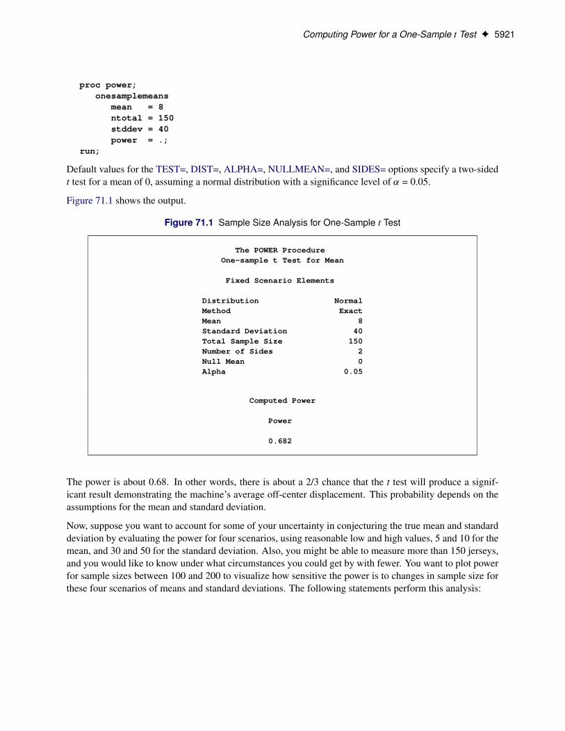
proc power;onesamplemeans
mean = 8ntotal = 150stddev = 40power = .;
run;
Default values for the TEST=, DIST=, ALPHA=, NULLMEAN=, and SIDES= options specify a two-sidedt test for a mean of 0, assuming a normal distribution with a significance level of ˛ = 0.05.
Figure 71.1 shows the output.
Figure 71.1 Sample Size Analysis for One-Sample t Test
The POWER ProcedureOne-sample t Test for Mean
Fixed Scenario Elements
Distribution NormalMethod ExactMean 8Standard Deviation 40Total Sample Size 150Number of Sides 2Null Mean 0Alpha 0.05
Computed Power
Power
0.682
The power is about 0.68. In other words, there is about a 2/3 chance that the t test will produce a signif-icant result demonstrating the machine’s average off-center displacement. This probability depends on theassumptions for the mean and standard deviation.
Now, suppose you want to account for some of your uncertainty in conjecturing the true mean and standarddeviation by evaluating the power for four scenarios, using reasonable low and high values, 5 and 10 for themean, and 30 and 50 for the standard deviation. Also, you might be able to measure more than 150 jerseys,and you would like to know under what circumstances you could get by with fewer. You want to plot powerfor sample sizes between 100 and 200 to visualize how sensitive the power is to changes in sample size forthese four scenarios of means and standard deviations. The following statements perform this analysis:

5922 F Chapter 71: The POWER Procedure
ods listing style=htmlbluecml;ods graphics on;
proc power;onesamplemeans
mean = 5 10ntotal = 150stddev = 30 50power = .;
plot x=n min=100 max=200;run;
ods graphics off;
The new mean and standard deviation values are specified by using the MEAN= and STDDEV= optionsin the ONESAMPLEMEANS statement. The PLOT statement with X=N produces a plot with sample sizeon the X axis. (The result parameter, in this case the power, is always plotted on the other axis.) TheMIN= and MAX= options in the PLOT statement determine the sample size range. The ODS GRAPHICSON statement enables ODS Graphics. The ODS LISTING STYLE=HTMLBLUECML statement specifiesthe HTMLBLUECML style, which is suitable for use with PROC POWER because it allows both markersymbols and line styles to vary. See the section “ODS Styles Suitable for Use with PROC POWER” onpage 6082 for more information.
Figure 71.2 shows the output, and Figure 71.3 shows the plot.
Figure 71.2 Sample Size Analysis for One-Sample t Test with Input Ranges
The POWER ProcedureOne-sample t Test for Mean
Fixed Scenario Elements
Distribution NormalMethod ExactTotal Sample Size 150Number of Sides 2Null Mean 0Alpha 0.05
Computed Power
StdIndex Mean Dev Power
1 5 30 0.5272 5 50 0.2293 10 30 0.9824 10 50 0.682

Determining Required Sample Size for a Two-Sample t Test F 5923
Figure 71.3 Plot of Power versus Sample Size for One-Sample t Test with Input Ranges
The power ranges from about 0.23 to 0.98 for a sample size of 150 depending on the mean and standarddeviation. In Figure 71.3, the line style identifies the mean, and the plotting symbol identifies the standarddeviation. The locations of plotting symbols indicate computed powers; the curves are linear interpolationsof these points. The plot suggests sufficient power for a mean of 10 and standard deviation of 30 (for any ofthe sample sizes) but insufficient power for the other three scenarios.
Determining Required Sample Size for a Two-Sample t TestIn this example you want to compare two physical therapy treatments designed to increase muscle flexibility.You need to determine the number of patients required to achieve a power of at least 0.9 to detect a groupmean difference in a two-sample t test. You will use ˛ D 0:05 (two-tailed).
5924 F Chapter 71: The POWER Procedure
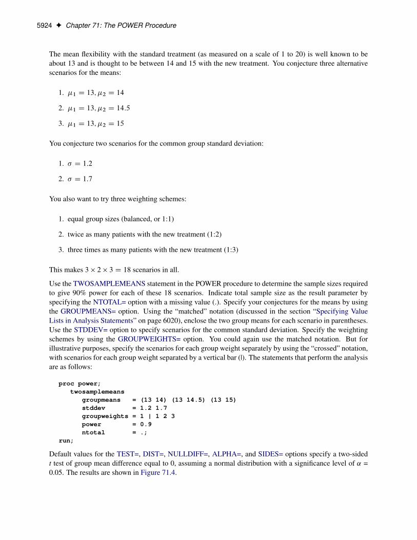
The mean flexibility with the standard treatment (as measured on a scale of 1 to 20) is well known to beabout 13 and is thought to be between 14 and 15 with the new treatment. You conjecture three alternativescenarios for the means:
1. �1 D 13; �2 D 14
2. �1 D 13; �2 D 14:5
3. �1 D 13; �2 D 15
You conjecture two scenarios for the common group standard deviation:
1. � D 1:2
2. � D 1:7
You also want to try three weighting schemes:
1. equal group sizes (balanced, or 1:1)
2. twice as many patients with the new treatment (1:2)
3. three times as many patients with the new treatment (1:3)
This makes 3 � 2 � 3 D 18 scenarios in all.
Use the TWOSAMPLEMEANS statement in the POWER procedure to determine the sample sizes requiredto give 90% power for each of these 18 scenarios. Indicate total sample size as the result parameter byspecifying the NTOTAL= option with a missing value (.). Specify your conjectures for the means by usingthe GROUPMEANS= option. Using the “matched” notation (discussed in the section “Specifying ValueLists in Analysis Statements” on page 6020), enclose the two group means for each scenario in parentheses.Use the STDDEV= option to specify scenarios for the common standard deviation. Specify the weightingschemes by using the GROUPWEIGHTS= option. You could again use the matched notation. But forillustrative purposes, specify the scenarios for each group weight separately by using the “crossed” notation,with scenarios for each group weight separated by a vertical bar (|). The statements that perform the analysisare as follows:
proc power;twosamplemeans
groupmeans = (13 14) (13 14.5) (13 15)stddev = 1.2 1.7groupweights = 1 | 1 2 3power = 0.9ntotal = .;
run;
Default values for the TEST=, DIST=, NULLDIFF=, ALPHA=, and SIDES= options specify a two-sidedt test of group mean difference equal to 0, assuming a normal distribution with a significance level of ˛ =0.05. The results are shown in Figure 71.4.

Determining Required Sample Size for a Two-Sample t Test F 5925
Figure 71.4 Sample Size Analysis for Two-Sample t Test Using Group Means
The POWER ProcedureTwo-Sample t Test for Mean Difference
Fixed Scenario Elements
Distribution NormalMethod ExactGroup 1 Weight 1Nominal Power 0.9Number of Sides 2Null Difference 0Alpha 0.05
Computed N Total
Std Actual NIndex Mean1 Mean2 Dev Weight2 Power Total
1 13 14.0 1.2 1 0.907 642 13 14.0 1.2 2 0.908 723 13 14.0 1.2 3 0.905 844 13 14.0 1.7 1 0.901 1245 13 14.0 1.7 2 0.905 1416 13 14.0 1.7 3 0.900 1647 13 14.5 1.2 1 0.910 308 13 14.5 1.2 2 0.906 339 13 14.5 1.2 3 0.916 40
10 13 14.5 1.7 1 0.900 5611 13 14.5 1.7 2 0.901 6312 13 14.5 1.7 3 0.908 7613 13 15.0 1.2 1 0.913 1814 13 15.0 1.2 2 0.927 2115 13 15.0 1.2 3 0.922 2416 13 15.0 1.7 1 0.914 3417 13 15.0 1.7 2 0.921 3918 13 15.0 1.7 3 0.910 44
The interpretation is that in the best-case scenario (large mean difference of 2, small standard deviation of1.2, and balanced design), a sample size of N = 18 (n1 D n2 D 9) patients is sufficient to achieve a powerof at least 0.9. In the worst-case scenario (small mean difference of 1, large standard deviation of 1.7, and a1:3 unbalanced design), a sample size of N = 164 (n1 D 41; n2 D 123) patients is necessary. The NominalPower of 0.9 in the “Fixed Scenario Elements” table represents the input target power, and the Actual Powercolumn in the “Computed N Total” table is the power at the sample size (N Total) adjusted to achieve thespecified sample weighting exactly.

5926 F Chapter 71: The POWER Procedure
Note the following characteristics of the analysis, and ways you can modify them if you want:
� The total sample sizes are rounded up to multiples of the weight sums (2 for the 1:1 design, 3 forthe 1:2 design, and 4 for the 1:3 design) to ensure that each group size is an integer. To request rawfractional sample size solutions, use the NFRACTIONAL option.
� Only the group weight that varies (the one for group 2) is displayed as an output column, while theweight for group 1 appears in the “Fixed Scenario Elements” table. To display the group weightstogether in output columns, use the matched version of the value list rather than the crossed version.
� If you can specify only differences between group means (instead of their individual values), or if youwant to display the mean differences instead of the individual means, use the MEANDIFF= optioninstead of the GROUPMEANS= option.
The following statements implement all of these modifications:
proc power;twosamplemeans
nfractionalmeandiff = 1 to 2 by 0.5stddev = 1.2 1.7groupweights = (1 1) (1 2) (1 3)power = 0.9ntotal = .;
run;
Figure 71.5 shows the new results.
Figure 71.5 Sample Size Analysis for Two-Sample t Test Using Mean Differences
The POWER ProcedureTwo-Sample t Test for Mean Difference
Fixed Scenario Elements
Distribution NormalMethod ExactNominal Power 0.9Number of Sides 2Null Difference 0Alpha 0.05

Syntax: POWER Procedure F 5927
Figure 71.5 continued
Computed Ceiling N Total
Mean Std Fractional Actual CeilingIndex Diff Dev Weight1 Weight2 N Total Power N Total
1 1.0 1.2 1 1 62.507429 0.902 632 1.0 1.2 1 2 70.065711 0.904 713 1.0 1.2 1 3 82.665772 0.901 834 1.0 1.7 1 1 123.418482 0.901 1245 1.0 1.7 1 2 138.598159 0.901 1396 1.0 1.7 1 3 163.899094 0.900 1647 1.5 1.2 1 1 28.961958 0.900 298 1.5 1.2 1 2 32.308867 0.906 339 1.5 1.2 1 3 37.893351 0.901 38
10 1.5 1.7 1 1 55.977156 0.900 5611 1.5 1.7 1 2 62.717357 0.901 6312 1.5 1.7 1 3 73.954291 0.900 7413 2.0 1.2 1 1 17.298518 0.913 1814 2.0 1.2 1 2 19.163836 0.913 2015 2.0 1.2 1 3 22.282926 0.910 2316 2.0 1.7 1 1 32.413512 0.905 3317 2.0 1.7 1 2 36.195531 0.907 3718 2.0 1.7 1 3 42.504535 0.903 43
Note that the Nominal Power of 0.9 applies to the raw computed sample size (Fractional N Total), and theActual Power column applies to the rounded sample size (Ceiling N Total). Some of the adjusted samplesizes in Figure 71.5 are lower than those in Figure 71.4 because underlying group sample sizes are allowedto be fractional (for example, the first Ceiling N Total of 63 corresponding to equal group sizes of 31.5).
Syntax: POWER ProcedureThe following statements are available in the POWER procedure:
PROC POWER < options > ;LOGISTIC < options > ;MULTREG < options > ;ONECORR < options > ;ONESAMPLEFREQ < options > ;ONESAMPLEMEANS < options > ;ONEWAYANOVA < options > ;PAIREDFREQ < options > ;PAIREDMEANS < options > ;PLOT < plot-options > < / graph-options > ;TWOSAMPLEFREQ < options > ;TWOSAMPLEMEANS < options > ;TWOSAMPLESURVIVAL < options > ;TWOSAMPLEWILCOXON < options > ;

5928 F Chapter 71: The POWER Procedure
The statements in the POWER procedure consist of the PROC POWER statement, a set of analysis state-ments (for requesting specific power and sample size analyses), and the PLOT statement (for produc-ing graphs). The PROC POWER statement and at least one of the analysis statements are required.The analysis statements are LOGISTIC, MULTREG, ONECORR, ONESAMPLEFREQ, ONESAMPLE-MEANS, ONEWAYANOVA, PAIREDFREQ, PAIREDMEANS, TWOSAMPLEFREQ, TWOSAMPLE-MEANS, TWOSAMPLESURVIVAL, and TWOSAMPLEWILCOXON.
You can use multiple analysis statements and multiple PLOT statements. Each analysis statement produces aseparate sample size analysis. Each PLOT statement refers to the previous analysis statement and generatesa separate graph (or set of graphs).
The name of an analysis statement describes the framework of the statistical analysis for which samplesize calculations are desired. You use options in the analysis statements to identify the result parameter tocompute, to specify the statistical test and computational options, and to provide one or more scenarios forthe values of relevant analysis parameters.
Table 71.1 summarizes the basic functions of each statement in PROC POWER. The syntax of each state-ment in Table 71.1 is described in the following pages.
Table 71.1 Statements in the POWER Procedure
Statement Description
PROC POWER Invokes the procedure
LOGISTIC Likelihood ratio chi-square test of a single predictor in logisticregression with binary response
MULTREG Tests of one or more coefficients in multiple linear regressionONECORR Fisher’s z test and t test of (partial) correlationONESAMPLEFREQ Tests, confidence interval precision, and equivalence tests of a
single binomial proportionONESAMPLEMEANS One-sample t test, confidence interval precision, or equivalence
testONEWAYANOVA One-way ANOVA including single-degree-of-freedom contrastsPAIREDFREQ McNemar’s test for paired proportionsPAIREDMEANS Paired t test, confidence interval precision, or equivalence test
PLOT Displays plots for previous sample size analysis
TWOSAMPLEFREQ Chi-square, likelihood ratio, and Fisher’s exact tests for twoindependent proportions
TWOSAMPLEMEANS Two-sample t test, confidence interval precision, or equivalencetest
TWOSAMPLESURVIVAL Log-rank, Gehan, and Tarone-Ware tests for comparing twosurvival curves
TWOSAMPLEWILCOXON Wilcoxon-Mann-Whitney (rank-sum) test for 2 independentgroups
See the section “Summary of Analyses” on page 6018 for a summary of the analyses available and thesyntax required for them.

PROC POWER Statement F 5929
PROC POWER StatementPROC POWER < options > ;
The PROC POWER statement invokes the POWER procedure. You can specify the following option.
PLOTONLYspecifies that only graphical results from the PLOT statement should be produced.
LOGISTIC StatementLOGISTIC < options > ;
The LOGISTIC statement performs power and sample size analyses for the likelihood ratio chi-square testof a single predictor in binary logistic regression, possibly in the presence of one or more covariates thatmight be correlated with the tested predictor.
Summary of Options
Table 71.2 summarizes the options available in the LOGISTIC statement.
Table 71.2 LOGISTIC Statement Options
Option Description
Define analysisTEST= Specifies the statistical analysis
Specify analysis informationALPHA= Specifies the significance levelCOVARIATES= Specifies the distributions of predictor variablesTESTPREDICTOR= Specifies the distribution of the predictor variable being testedVARDIST= Defines a distribution for a predictor variable
Specify effectsCORR= Specifies the multiple correlation between the predictor and the covariatesCOVODDSRATIOS= Specifies the odds ratios for the covariatesCOVREGCOEFFS= Specifies the regression coefficients for the covariatesDEFAULTUNIT= Specifies the default change in the predictor variablesINTERCEPT= Specifies the interceptRESPONSEPROB= Specifies the response probabilityTESTODDSRATIO= Specifies the odds ratio being testedTESTREGCOEFF= Specifies the regression coefficient for the predictor variableUNITS= Specifies the changes in the predictor variables
Specify sample sizeNFRACTIONAL Enables fractional input and output for sample sizesNTOTAL= Specifies the sample size
Specify powerPOWER= Specifies the desired power of the test

5930 F Chapter 71: The POWER Procedure
Table 71.2 continued
Option Description
Specify computational methodDEFAULTNBINS= Specifies the default number of categories for each predictor variableNBINS= Specifies the number of categories for predictor variables
Control ordering in outputOUTPUTORDER= Controls the output order of parameters
Table 71.3 summarizes the valid result parameters in the LOGISTIC statement.
Table 71.3 Summary of Result Parameters in the LOGISTIC Statement
Analyses Solve For Syntax
TEST=LRCHI Power POWER=.Sample size NTOTAL=.
Dictionary of Options
ALPHA=number-listspecifies the level of significance of the statistical test. The default is 0.05, corresponding to theusual 0.05 � 100% = 5% level of significance. See the section “Specifying Value Lists in AnalysisStatements” on page 6020 for information about specifying the number-list.
CORR=number-listspecifies the multiple correlation (�) between the tested predictor and the covariates. If you also spec-ify the COVARIATES= option, then the sample size is either multiplied (if you are computing power)or divided (if you are computing sample size) by a factor of .1 � �2/. See the section “SpecifyingValue Lists in Analysis Statements” on page 6020 for information about specifying the number-list.
COVARIATES=grouped-name-listspecifies the distributions of any predictor variables in the model but not being tested, using labelsspecified with the VARDIST= option. The distributions are assumed to be independent of each otherand of the tested predictor. If this option is omitted, then the tested predictor specified by the TEST-EDPREDICTOR= option is assumed to be the only predictor in the model. See the section “Specify-ing Value Lists in Analysis Statements” on page 6020 for information about specifying the grouped-name-list.
COVODDSRATIOS=grouped-number-listspecifies the odds ratios for the covariates in the full model (including variables in the TESTPREDIC-TOR= and COVARIATES= options). The ordering of the values corresponds to the ordering in theCOVARIATES= option. If the response variable is coded as Y = 1 for success and Y = 0 for failure,then the odds ratio for each covariate X is the odds of Y = 1 when X D a divided by the odds of Y= 1 when X D b, where a and b are determined from the DEFAULTUNIT= and UNITS= options.Values must be greater than zero. See the section “Specifying Value Lists in Analysis Statements” onpage 6020 for information about specifying the grouped-number-list.

LOGISTIC Statement F 5931
COVREGCOEFFS=grouped-number-listspecifies the regression coefficients for the covariates in the full model including the test predictor (asspecified by the TESTPREDICTOR= option). The ordering of the values corresponds to the orderingin the COVARIATES= option. See the section “Specifying Value Lists in Analysis Statements” onpage 6020 for information about specifying the grouped-number-list.
DEFAULTNBINS=numberspecifies the default number of categories (or “bins”) into which the distribution for each predictorvariable is divided in internal calculations. Higher values increase computational time and memoryrequirements but generally lead to more accurate results. Each test predictor or covariate that isabsent from the NBINS= option derives its bin number from the DEFAULTNBINS= option. Thedefault value is DEFAULTNBINS=10.
There are two variable distributions for which the number of bins can be overridden internally:
� For an ordinal distribution, the number of ordinal values is always used as the number of bins.
� For a binomial distribution, if the requested number of bins is larger than n + 1, where n is thesample size parameter of the binomial distribution, then exactly n + 1 bins are used.
DEFAULTUNIT=change-specspecifies the default change in the predictor variables assumed for odds ratios specified with the COV-ODDSRATIOS= and TESTODDSRATIO= options. Each test predictor or covariate that is absentfrom the UNITS= option derives its change value from the DEFAULTUNIT= option. The value mustbe nonzero. The default value is DEFAULTUNIT=1. This option can be used only if at least one ofthe COVODDSRATIOS= and TESTODDSRATIO= options is used.
Valid specifications for change-spec are as follows:
number defines the odds ratio as the ratio of the response variable odds when X D a to the oddswhen X D a � number for any constant a.
<+ | ->SD defines the odds ratio as the ratio of the odds when X D a to the odds when X D a � �(or X D a C � , if SD is preceded by a minus sign (–)) for any constant a, where � is thestandard deviation of X (as determined from the VARDIST= option).
multiple*SD defines the odds ratio as the ratio of the odds when X D a to the odds when X Da�multiple �� for any constant a, where � is the standard deviation of X (as determined fromthe VARDIST= option).
PERCENTILES(p1, p2) defines the odds ratio as the ratio of the odds when X is equal to its p2 �100th percentile to the odds when X is equal to its p1�100th percentile (where the percentilesare determined from the distribution specified in the VARDIST= option). Values for p1 and p2must be strictly between 0 and 1.
INTERCEPT=number-listspecifies the intercept in the full model (including variables in the TESTPREDICTOR= and COVARI-ATES= options). See the section “Specifying Value Lists in Analysis Statements” on page 6020 forinformation about specifying the number-list.

5932 F Chapter 71: The POWER Procedure
NBINS=(“name” = number < . . . "name" = number >)specifies the number of categories (or “bins”) into which the distribution for each predictor variable(identified by its name from the VARDIST= option) is divided in internal calculations. Higher valuesincrease computational time and memory requirements but generally lead to more accurate results.Each predictor variable that is absent from the NBINS= option derives its bin number from the DE-FAULTNBINS= option.
There are two variable distributions for which the NBINS= value can be overridden internally:
� For an ordinal distribution, the number of ordinal values is always used as the number of bins.� For a binomial distribution, if the requested number of bins is larger than n + 1, where n is the
sample size parameter of the binomial distribution, then exactly n + 1 bins are used.
NFRACTIONALNFRAC
enables fractional input and output for sample sizes. See the section “Sample Size Adjustment Op-tions” on page 6023 for information about the ramifications of the presence (and absence) of theNFRACTIONAL option.
NTOTAL=number-listspecifies the sample size or requests a solution for the sample size with a missing value (NTOTAL=.).Values must be at least one. See the section “Specifying Value Lists in Analysis Statements” onpage 6020 for information about specifying the number-list.
OUTPUTORDER=INTERNALOUTPUTORDER=REVERSEOUTPUTORDER=SYNTAX
controls how the input and default analysis parameters are ordered in the output. OUT-PUTORDER=INTERNAL (the default) arranges the parameters in the output according to thefollowing order of their corresponding options:
� DEFAULTNBINS=� NBINS=� ALPHA=� RESPONSEPROB=� INTERCEPT=� TESTPREDICTOR=� TESTODDSRATIO=� TESTREGCOEFF=� COVARIATES=� COVODDSRATIOS=� COVREGCOEFFS=� CORR=� NTOTAL=� POWER=
The OUTPUTORDER=SYNTAX option arranges the parameters in the output in the same or-der in which their corresponding options are specified in the LOGISTIC statement. The OUT-PUTORDER=REVERSE option arranges the parameters in the output in the reverse of the orderin which their corresponding options are specified in the LOGISTIC statement.

LOGISTIC Statement F 5933
POWER=number-listspecifies the desired power of the test or requests a solution for the power with a missing value(POWER=.). The power is expressed as a probability, a number between 0 and 1, rather than asa percentage. See the section “Specifying Value Lists in Analysis Statements” on page 6020 forinformation about specifying the number-list.
RESPONSEPROB=number-listspecifies the response probability in the full model when all predictor variables (including variables inthe TESTPREDICTOR= and COVARIATES= options) are equal to their means. The log odds of thisprobability are equal to the intercept in the full model where all predictor are centered at their means.If the response variable is coded as Y = 1 for success and Y = 0 for failure, then this probability isequal to the mean of Y in the full model when all Xs are equal to their means. Values must be strictlybetween zero and one. See the section “Specifying Value Lists in Analysis Statements” on page 6020for information about specifying the number-list.
TEST=LRCHIspecifies the likelihood ratio chi-square test of a single model parameter in binary logistic regression.This is the default test option.
TESTODDSRATIO=number-listspecifies the odds ratio for the predictor variable being tested in the full model (including variables inthe TESTPREDICTOR= and COVARIATES= options). If the response variable is coded as Y = 1 forsuccess and Y = 0 for failure, then the odds ratio for the X being tested is the odds of Y = 1 whenX D adivided by the odds of Y = 1 when X D b, where a and b are determined from the DEFAULTUNIT=and UNITS= options. Values must be greater than zero. See the section “Specifying Value Lists inAnalysis Statements” on page 6020 for information about specifying the number-list.
TESTPREDICTOR=name-listspecifies the distribution of the predictor variable being tested, using labels specified with theVARDIST= option. This distribution is assumed to be independent of the distributions of the co-variates as defined in the COVARIATES= option. See the section “Specifying Value Lists in AnalysisStatements” on page 6020 for information about specifying the name-list.
TESTREGCOEFF=number-listspecifies the regression coefficient for the predictor variable being tested in the full model includingthe covariates specified by the COVARIATES= option. See the section “Specifying Value Lists inAnalysis Statements” on page 6020 for information about specifying the number-list.
UNITS=(“name” = change-spec < . . . "name" = change-spec >)specifies the changes in the predictor variables assumed for odds ratios specified with the COV-ODDSRATIOS= and TESTODDSRATIO= options. Each predictor variable whose name (fromthe VARDIST= option) is absent from the UNITS option derives its change value from the DE-FAULTUNIT= option. This option can be used only if at least one of the COVODDSRATIOS= andTESTODDSRATIO= options is used.
Valid specifications for change-spec are as follows:
number defines the odds ratio as the ratio of the response variable odds when X D a to the oddswhen X D a � number for any constant a.

5934 F Chapter 71: The POWER Procedure
<+ | ->SD defines the odds ratio as the ratio of the odds when X D a to the odds when X D a � �(or X D a C � , if SD is preceded by a minus sign (–)) for any constant a, where � is thestandard deviation of X (as determined from the VARDIST= option).
multiple*SD defines the odds ratio as the ratio of the odds when X D a to the odds when X Da�multiple �� for any constant a, where � is the standard deviation of X (as determined fromthe VARDIST= option).
PERCENTILES(p1, p2) defines the odds ratio as the ratio of the odds when X is equal to its p2 �100th percentile to the odds when X is equal to its p1�100th percentile (where the percentilesare determined from the distribution specified in the VARDIST= option). Values for p1 and p2must be strictly between 0 and 1.
Each unit value must be nonzero.
VARDIST("label")=distribution (parameters)defines a distribution for a predictor variable.
For the VARDIST= option,
label identifies the variable distribution in the output and with the COVARIATES= andTESTPREDICTOR= options.
distribution specifies the distributional form of the variable.
parameters specifies one or more parameters associated with the distribution.
Choices for distributional forms and their parameters are as follows:
ORDINAL ((values) : (probabilities)) is an ordered categorical distribution. The values are anynumbers separated by spaces. The probabilities are numbers between 0 and 1 (inclusive) sep-arated by spaces. Their sum must be exactly 1. The number of probabilities must match thenumber of values.
BETA (a, b <, l, r >) is a beta distribution with shape parameters a and b and optional location pa-rameters l and r. The values of a and b must be greater than 0, and l must be less than r. Thedefault values for l and r are 0 and 1, respectively.
BINOMIAL (p, n) is a binomial distribution with probability of success p and number of indepen-dent Bernoulli trials n. The value of p must be greater than 0 and less than 1, and n must be aninteger greater than 0. If n = 1, then the distribution is binary.
EXPONENTIAL (�) is an exponential distribution with scale �, which must be greater than 0.
GAMMA (a, �) is a gamma distribution with shape a and scale �. The values of a and � must begreater than 0.
LAPLACE (� , �) is a Laplace distribution with location � and scale �. The value of � must begreater than 0.
LOGISTIC (� , �) is a logistic distribution with location � and scale �. The value of � must begreater than 0.
LOGNORMAL (� , �) is a lognormal distribution with location � and scale �. The value of � mustbe greater than 0.
LOGISTIC Statement F 5935
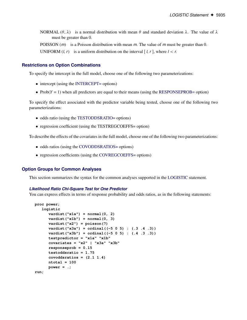
NORMAL (� , �) is a normal distribution with mean � and standard deviation �. The value of �must be greater than 0.
POISSON (m) is a Poisson distribution with mean m. The value of m must be greater than 0.
UNIFORM (l, r ) is a uniform distribution on the interval Œ l, r �, where l < r.
Restrictions on Option Combinations
To specify the intercept in the full model, choose one of the following two parameterizations:
� intercept (using the INTERCEPT= options)
� Prob(Y = 1) when all predictors are equal to their means (using the RESPONSEPROB= option)
To specify the effect associated with the predictor variable being tested, choose one of the following twoparameterizations:
� odds ratio (using the TESTODDSRATIO= options)
� regression coefficient (using the TESTREGCOEFFS= option)
To describe the effects of the covariates in the full model, choose one of the following two parameterizations:
� odds ratios (using the COVODDSRATIOS= options)
� regression coefficients (using the COVREGCOEFFS= options)
Option Groups for Common Analyses
This section summarizes the syntax for the common analyses supported in the LOGISTIC statement.
Likelihood Ratio Chi-Square Test for One PredictorYou can express effects in terms of response probability and odds ratios, as in the following statements:
proc power;logistic
vardist("x1a") = normal(0, 2)vardist("x1b") = normal(0, 3)vardist("x2") = poisson(7)vardist("x3a") = ordinal((-5 0 5) : (.3 .4 .3))vardist("x3b") = ordinal((-5 0 5) : (.4 .3 .3))testpredictor = "x1a" "x1b"covariates = "x2" | "x3a" "x3b"responseprob = 0.15testoddsratio = 1.75covoddsratios = (2.1 1.4)ntotal = 100power = .;
run;

5936 F Chapter 71: The POWER Procedure
The VARDIST= options define the distributions of the predictor variables. The TESTPREDICTOR= optionspecifies two scenarios for the test predictor distribution, Normal(10,2) and Normal(10,3). The COVARI-ATES= option specifies two covariates, the first with a Poisson(7) distribution. The second covariate has anordinal distribution on the values –5, 0, and 5 with two scenarios for the associated probabilities: (.3, .4, .3)and (.4, .3, .3). The response probability in the full model with all variables equal to zero is specified bythe RESPONSEPROB= option as 0.15. The odds ratio for a unit decrease in the tested predictor is specifiedby the TESTODDSRATIO= option to be 1.75. Corresponding odds ratios for the two covariates in the fullmodel are specified by the COVODDSRATIOS= option to be 2.1 and 1.4. The POWER=. option requests asolution for the power at a sample size of 100 as specified by the NTOTAL= option.
Default values of the TEST= and ALPHA= options specify a likelihood ratio test of the first predictor witha significance level of 0.05. The default of DEFAULTUNIT=1 specifies that all odds ratios are defined interms of unit changes in predictors. The default of DEFAULTNBINS=10 specifies that each of the threepredictor variables is discretized into a distribution with 10 categories in internal calculations.
You can also express effects in terms of regression coefficients, as in the following statements:
proc power;logistic
vardist("x1a") = normal(0, 2)vardist("x1b") = normal(0, 3)vardist("x2") = poisson(7)vardist("x3a") = ordinal((-5 0 5) : (.3 .4 .3))vardist("x3b") = ordinal((-5 0 5) : (.4 .3 .3))testpredictor = "x1a" "x1b"covariates = "x2" | "x3a" "x3b"intercept = -6.928162testregcoeff = 0.5596158covregcoeffs = (0.7419373 0.3364722)ntotal = 100power = .;
run;
The regression coefficients for the tested predictor (TESTREGCOEFF=0.5596158) and covariates (COV-REGCOEFFS=(0.7419373 0.3364722)) are determined by taking the logarithm of the corresponding oddsratios. The intercept in the full model is specified as –6.928162 by the INTERCEPT= option. This numberis calculated according to the formula at the end of “Analyses in the LOGISTIC Statement” on page 6029,which expresses the intercept in terms of the response probability, regression coefficients, and predictormeans:
Intercept D log�
0:15
1 � 0:15
�� .0:5596158.0/C 0:7419373.7/C 0:3364722.0//
MULTREG StatementMULTREG < options > ;
The MULTREG statement performs power and sample size analyses for Type III F tests of sets of predictorsin multiple linear regression, assuming either fixed or normally distributed predictors.
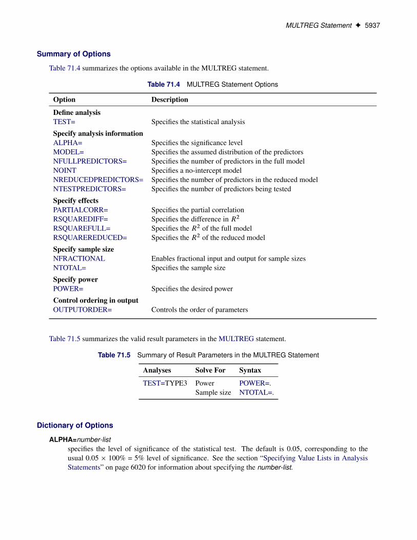
MULTREG Statement F 5937
Summary of Options
Table 71.4 summarizes the options available in the MULTREG statement.
Table 71.4 MULTREG Statement Options
Option Description
Define analysisTEST= Specifies the statistical analysis
Specify analysis informationALPHA= Specifies the significance levelMODEL= Specifies the assumed distribution of the predictorsNFULLPREDICTORS= Specifies the number of predictors in the full modelNOINT Specifies a no-intercept modelNREDUCEDPREDICTORS= Specifies the number of predictors in the reduced modelNTESTPREDICTORS= Specifies the number of predictors being tested
Specify effectsPARTIALCORR= Specifies the partial correlationRSQUAREDIFF= Specifies the difference in R2
RSQUAREFULL= Specifies the R2 of the full modelRSQUAREREDUCED= Specifies the R2 of the reduced model
Specify sample sizeNFRACTIONAL Enables fractional input and output for sample sizesNTOTAL= Specifies the sample size
Specify powerPOWER= Specifies the desired power
Control ordering in outputOUTPUTORDER= Controls the order of parameters
Table 71.5 summarizes the valid result parameters in the MULTREG statement.
Table 71.5 Summary of Result Parameters in the MULTREG Statement
Analyses Solve For Syntax
TEST=TYPE3 Power POWER=.Sample size NTOTAL=.
Dictionary of Options
ALPHA=number-listspecifies the level of significance of the statistical test. The default is 0.05, corresponding to theusual 0.05 � 100% = 5% level of significance. See the section “Specifying Value Lists in AnalysisStatements” on page 6020 for information about specifying the number-list.

5938 F Chapter 71: The POWER Procedure
MODEL=keyword-listspecifies the assumed distribution of the tested predictors. MODEL=FIXED indicates a fixed predic-tor distribution. MODEL=RANDOM (the default) indicates a joint multivariate normal distributionfor the response and tested predictors. You can use the aliases CONDITIONAL for FIXED and UN-CONDITIONAL for RANDOM. See the section “Specifying Value Lists in Analysis Statements” onpage 6020 for information about specifying the keyword-list.
FIXED fixed predictors
RANDOM random (multivariate normal) predictors
NFRACTIONAL
NFRACenables fractional input and output for sample sizes. See the section “Sample Size Adjustment Op-tions” on page 6023 for information about the ramifications of the presence (and absence) of theNFRACTIONAL option.
NFULLPREDICTORS=number-list
NFULLPRED=number-listspecifies the number of predictors in the full model, not counting the intercept. See the section“Specifying Value Lists in Analysis Statements” on page 6020 for information about specifying thenumber-list.
NOINTspecifies a no-intercept model (for both full and reduced models). By default, the intercept is includedin the model. If you want to test the intercept, you can specify the NOINT option and simply considerthe intercept to be one of the predictors being tested. See the section “Specifying Value Lists inAnalysis Statements” on page 6020 for information about specifying the number-list.
NREDUCEDPREDICTORS=number-list
NREDUCEDPRED=number-list
NREDPRED=number-listspecifies the number of predictors in the reduced model, not counting the intercept. This is the sameas the difference between values of the NFULLPREDICTORS= and NTESTPREDICTORS= op-tions. Note that supplying a value of 0 is the same as specifying an F test of a Pearson correlation.This option cannot be used at the same time as the NTESTPREDICTORS= option. See the section“Specifying Value Lists in Analysis Statements” on page 6020 for information about specifying thenumber-list.
NTESTPREDICTORS=number-list
NTESTPRED=number-listspecifies the number of predictors being tested. This is the same as the difference between val-ues of the NFULLPREDICTORS= and NREDUCEDPREDICTORS= options. Note that supplyingidentical values for the NTESTPREDICTORS= and NFULLPREDICTORS= options is the same asspecifying an F test of a Pearson correlation. This option cannot be used at the same time as the NRE-DUCEDPREDICTORS= option. See the section “Specifying Value Lists in Analysis Statements” onpage 6020 for information about specifying the number-list.

MULTREG Statement F 5939
NTOTAL=number-listspecifies the sample size or requests a solution for the sample size with a missing value (NTOTAL=.).The minimum acceptable value for the sample size depends on the MODEL=, NOINT, NFULLPRE-DICTORS=, NTESTPREDICTORS=, and NREDUCEDPREDICTORS= options. It ranges from p+ 1 to p + 3, where p is the value of the NFULLPREDICTORS option. See Table 71.30 for furtherinformation about minimum NTOTAL values, and see the section “Specifying Value Lists in AnalysisStatements” on page 6020 for information about specifying the number-list.
OUTPUTORDER=INTERNALOUTPUTORDER=REVERSEOUTPUTORDER=SYNTAX
controls how the input and default analysis parameters are ordered in the output. OUT-PUTORDER=INTERNAL (the default) arranges the parameters in the output according to thefollowing order of their corresponding options:
� MODEL=� NFULLPREDICTORS=� NTESTPREDICTORS=� NREDUCEDPREDICTORS=� ALPHA=� PARTIALCORR=� RSQUAREFULL=� RSQUAREREDUCED=� RSQUAREDIFF=� NTOTAL=� POWER=
The OUTPUTORDER=SYNTAX option arranges the parameters in the output in the same or-der in which their corresponding options are specified in the MULTREG statement. The OUT-PUTORDER=REVERSE option arranges the parameters in the output in the reverse of the orderin which their corresponding options are specified in the MULTREG statement.
PARTIALCORR=number-listPCORR=number-list
specifies the partial correlation between the tested predictors and the response, adjusting for any otherpredictors in the model. See the section “Specifying Value Lists in Analysis Statements” on page 6020for information about specifying the number-list.
POWER=number-listspecifies the desired power of the test or requests a solution for the power with a missing value(POWER=.). The power is expressed as a probability, a number between 0 and 1, rather than asa percentage. See the section “Specifying Value Lists in Analysis Statements” on page 6020 forinformation about specifying the number-list.
RSQUAREDIFF=number-listRSQDIFF=number-list
specifies the difference inR2 between the full and reduced models. This is equivalent to the proportionof variation explained by the predictors you are testing. It is also equivalent to the squared semipartialcorrelation of the tested predictors with the response. See the section “Specifying Value Lists inAnalysis Statements” on page 6020 for information about specifying the number-list.

5940 F Chapter 71: The POWER Procedure
RSQUAREFULL=number-list
RSQFULL=number-listspecifies the R2 of the full model, where R2 is the proportion of variation explained by the model.See the section “Specifying Value Lists in Analysis Statements” on page 6020 for information aboutspecifying the number-list.
RSQUAREREDUCED=number-list
RSQREDUCED=number-list
RSQRED=number-listspecifies theR2 of the reduced model, whereR2 is the proportion of variation explained by the model.If the reduced model is an empty or intercept-only model (in other words, if NREDUCEDPREDIC-TORS=0 or NTESTPREDICTORS=NFULLPREDICTORS), then RSQUAREREDUCED=0 is as-sumed. See the section “Specifying Value Lists in Analysis Statements” on page 6020 for informationabout specifying the number-list.
TEST=TYPE3specifies a Type III F test of a set of predictors adjusting for any other predictors in the model. Thisis the default test option.
Restrictions on Option Combinations
To specify the number of predictors, use any two of these three options:
� the number of predictors in the full model (NFULLPREDICTORS=)
� the number of predictors in the reduced model (NREDUCEDPREDICTORS=)
� the number of predictors being tested (NTESTPREDICTORS=)
To specify the effect, choose one of the following parameterizations:
� partial correlation (by using the PARTIALCORR= option)
� R2 for the full and reduced models (by using any two of RSQUAREDIFF=, RSQUAREFULL=, andRSQUAREREDUCED=)
Option Groups for Common Analyses
This section summarizes the syntax for the common analyses supported in the MULTREG statement.
Type III F Test of a Set of PredictorsYou can express effects in terms of partial correlation, as in the following statements. Default values ofthe TEST=, MODEL=, and ALPHA= options specify a Type III F test with a significance level of 0.05,assuming normally distributed predictors.

ONECORR Statement F 5941
proc power;multreg
model = randomnfullpredictors = 7ntestpredictors = 3partialcorr = 0.35ntotal = 100power = .;
run;
You can also express effects in terms of R2:
proc power;multreg
model = fixednfullpredictors = 7ntestpredictors = 3rsquarefull = 0.9rsquarediff = 0.1ntotal = .power = 0.9;
run;
ONECORR StatementONECORR < options > ;
The ONECORR statement performs power and sample size analyses for tests of simple and partial Pearsoncorrelation between two variables. Both Fisher’s z test and the t test are supported.
Summary of Options
Table 71.6 summarizes the options available in the ONECORR statement.
Table 71.6 ONECORR Statement Options
Option Description
Define analysisDIST= Specifies the underlying distribution assumed for the test statisticTEST= Specifies the statistical analysis
Specify analysis informationALPHA= Specifies the significance levelMODEL= Specifies the assumed distribution of the variablesNPARTIALVARS= Specifies the number of variables adjusted for in the correlationNULLCORR= Specifies the null value of the correlationSIDES= Specifies the number of sides and the direction of the statistical test
Specify effectsCORR= Specifies the correlation

5942 F Chapter 71: The POWER Procedure
Table 71.6 continued
Option Description
Specify sample sizeNFRACTIONAL Enables fractional input and output for sample sizesNTOTAL= Specifies the sample size
Specify powerPOWER= Specifies the desired power of the test
Control ordering in outputOUTPUTORDER= Controls the output order of parameters
Table 71.7 summarizes the valid result parameters in the ONECORR statement.
Table 71.7 Summary of Result Parameters in the ONECORR Statement
Analyses Solve For Syntax
TEST=PEARSON Power POWER=.Sample size NTOTAL=.
Dictionary of Options
ALPHA=number-listspecifies the level of significance of the statistical test. The default is 0.05, corresponding to theusual 0.05 � 100% = 5% level of significance. See the section “Specifying Value Lists in AnalysisStatements” on page 6020 for information about specifying the number-list.
CORR=number-listspecifies the correlation between two variables, possibly adjusting for other variables as determinedby the NPARTIALVARS= option. See the section “Specifying Value Lists in Analysis Statements”on page 6020 for information about specifying the number-list.
DIST=FISHERZ
DIST=Tspecifies the underlying distribution assumed for the test statistic. FISHERZ corresponds to Fisher’sz normalizing transformation of the correlation coefficient. T corresponds to the t transformation ofthe correlation coefficient. Note that DIST=T is equivalent to analyses in the MULTREG statementwith NTESTPREDICTORS=1. The default value is FISHERZ.
MODEL=keyword-listspecifies the assumed distribution of the first variable when DIST=T. The second variable is assumedto have a normal distribution. MODEL=FIXED indicates a fixed distribution. MODEL=RANDOM(the default) indicates a joint bivariate normal distribution with the second variable. You can use thealiases CONDITIONAL for FIXED and UNCONDITIONAL for RANDOM. This option can be usedonly for DIST=T. See the section “Specifying Value Lists in Analysis Statements” on page 6020 forinformation about specifying the keyword-list.

ONECORR Statement F 5943
FIXED fixed variables
RANDOM random (bivariate normal) variables
NFRACTIONAL
NFRACenables fractional input and output for sample sizes. See the section “Sample Size Adjustment Op-tions” on page 6023 for information about the ramifications of the presence (and absence) of theNFRACTIONAL option.
NPARTIALVARS=number-list
NPVARS=number-listspecifies the number of variables adjusted for in the correlation between the two primary variables.The default value is 0, corresponding to a simple correlation. See the section “Specifying Value Listsin Analysis Statements” on page 6020 for information about specifying the number-list.
NTOTAL=number-listspecifies the sample size or requests a solution for the sample size with a missing value (NTOTAL=.).Values for the sample size must be at least p + 3 when DIST=T and MODEL=CONDITIONAL, and atleast p + 4 when either DIST=FISHER or when DIST=T and MODEL=UNCONDITIONAL, wherep is the value of the NPARTIALVARS option. See the section “Specifying Value Lists in AnalysisStatements” on page 6020 for information about specifying the number-list.
NULLCORR=number-list
NULLC=number-listspecifies the null value of the correlation. The default value is 0. This option can be used only withthe DIST=FISHERZ analysis. See the section “Specifying Value Lists in Analysis Statements” onpage 6020 for information about specifying the number-list.
OUTPUTORDER=INTERNAL
OUTPUTORDER=REVERSE
OUTPUTORDER=SYNTAXcontrols how the input and default analysis parameters are ordered in the output. OUT-PUTORDER=INTERNAL (the default) arranges the parameters in the output according to thefollowing order of their corresponding options:
� MODEL=� SIDES=� NULL=� ALPHA=� NPARTIALVARS=� CORR=� NTOTAL=� POWER=
The OUTPUTORDER=SYNTAX option arranges the parameters in the output in the same or-der in which their corresponding options are specified in the ONECORR statement. The OUT-PUTORDER=REVERSE option arranges the parameters in the output in the reverse of the orderin which their corresponding options are specified in the ONECORR statement.

5944 F Chapter 71: The POWER Procedure
POWER=number-listspecifies the desired power of the test or requests a solution for the power with a missing value(POWER=.). The power is expressed as a probability, a number between 0 and 1, rather than asa percentage. See the section “Specifying Value Lists in Analysis Statements” on page 6020 forinformation about specifying the number-list.
SIDES=keyword-listspecifies the number of sides (or tails) and the direction of the statistical test. Valid keywords are
1 one-sided with alternative hypothesis in same direction as effect
2 two-sided
U upper one-sided with alternative greater than null value
L lower one-sided with alternative less than null value
The default value is 2.
TEST=PEARSONspecifies a test of the Pearson correlation coefficient between two variables, possibly adjusting forother variables. This is the default test option.
Option Groups for Common Analyses
This section summarizes the syntax for the common analyses supported in the ONECORR statement.
Fisher’s z Test for Pearson CorrelationThe following statements demonstrate a power computation for Fisher’s z test for correlation. Default valuesof TEST=PEARSON, ALPHA=0.05, SIDES=2, and NPARTIALVARS=0 are assumed.
proc power;onecorr dist=fisherz
nullcorr = 0.15corr = 0.35ntotal = 180power = .;
run;
t Test for Pearson CorrelationThe following statements demonstrate a sample size computation for the t test for correlation. Default valuesof TEST=PEARSON, MODEL=RANDOM, ALPHA=0.05, and SIDES=2 are assumed.
proc power;onecorr dist=t
npartialvars = 4corr = 0.45ntotal = .power = 0.85;
run;

ONESAMPLEFREQ Statement F 5945
ONESAMPLEFREQ StatementONESAMPLEFREQ < options > ;
The ONESAMPLEFREQ statement performs power and sample size analyses for exact and approximatetests (including equivalence, noninferiority, and superiority) and confidence interval precision for a singlebinomial proportion.
Summary of Options
Table 71.8 summarizes the options available in the ONESAMPLEFREQ statement.
Table 71.8 ONESAMPLEFREQ Statement Options
Option Description
Define analysisCI= Specifies an analysis of precision of a confidence intervalTEST= Specifies the statistical analysis
Specify analysis informationALPHA= Specifies the significance levelEQUIVBOUNDS= Specifies the lower and upper equivalence boundsLOWER= Specifies the lower equivalence boundMARGIN= Specifies the equivalence or noninferiority or superiority marginNULLPROPORTION= Specifies the null proportionSIDES= Specifies the number of sides and the direction of the statistical testUPPER= Specifies the upper equivalence bound
Specify effectHALFWIDTH= Specifies the desired confidence interval half-widthPROPORTION= Specifies the binomial proportion
Specify variance estimationVAREST= Specifies how the variance is computed
Specify sample sizeNFRACTIONAL Enables fractional input and output for sample sizesNTOTAL= Specifies the sample size
Specify power and related probabilitiesPOWER= Specifies the desired power of the testPROBWIDTH= Specifies the probability of obtaining a confidence interval half-width less
than or equal to the value specified by HALFWIDTH=
Choose computational methodMETHOD= Specifies the computational method
Control ordering in outputOUTPUTORDER= Controls the output order of parameters

5946 F Chapter 71: The POWER Procedure
Table 71.9 summarizes the valid result parameters for different analyses in the ONESAMPLEFREQ state-ment.
Table 71.9 Summary of Result Parameters in the ONESAMPLEFREQ Statement
Analyses Solve For Syntax
CI=WILSON Prob(width) PROBWIDTH=.
CI=AGRESTICOULL Prob(width) PROBWIDTH=.
CI=JEFFREYS Prob(width) PROBWIDTH=.
CI=EXACT Prob(width) PROBWIDTH=.
CI=WALD Prob(width) PROBWIDTH=.
CI=WALD_CORRECT Prob(width) PROBWIDTH=.
TEST=ADJZ METHOD=EXACT Power POWER=.
TEST=ADJZ METHOD=NORMAL Power POWER=.Sample size NTOTAL=.
TEST=EQUIV_ADJZ METHOD=EXACT Power POWER=.
TEST=EQUIV_ADJZ METHOD=NORMAL Power POWER=.Sample size NTOTAL=.
TEST=EQUIV_EXACT Power POWER=.
TEST=EQUIV_Z METHOD=EXACT Power POWER=.
TEST=EQUIV_Z METHOD=NORMAL Power POWER=.Sample size NTOTAL=.
TEST=EXACT Power POWER=.
TEST=Z METHOD=EXACT Power POWER=.
TEST=Z METHOD=NORMAL Power POWER=.Sample size NTOTAL=.
Dictionary of Options
ALPHA=number-listspecifies the level of significance of the statistical test. The default is 0.05, corresponding to the usual0.05 � 100% = 5% level of significance. If the CI= and SIDES=1 options are used, then the valuemust be less than 0.5. See the section “Specifying Value Lists in Analysis Statements” on page 6020for information about specifying the number-list.
CICI=AGRESTICOULL | ACCI=JEFFREYSCI=EXACT | CLOPPERPEARSON | CPCI=WALDCI=WALD_CORRECTCI=WILSON | SCORE
specifies an analysis of precision of a confidence interval for the sample binomial proportion.

ONESAMPLEFREQ Statement F 5947
The value of the CI= option specifies the type of confidence interval. The CI=AGRESTICOULLoption is a generalization of the “Adjusted Wald / add 2 successes and 2 failures” interval of Agrestiand Coull (1998) and is presented in Brown, Cai, and DasGupta (2001). It corresponds to the TA-BLES / BINOMIAL (AGRESTICOULL) option in PROC FREQ. The CI=JEFFREYS option spec-ifies the equal-tailed Jeffreys prior Bayesian interval, corresponding to the TABLES / BINOMIAL(JEFFREYS) option in PROC FREQ. The CI=EXACT option specifies the exact Clopper-Pearsonconfidence interval based on enumeration, corresponding to the TABLES / BINOMIAL (EXACT)option in PROC FREQ. The CI=WALD option specifies the confidence interval based on the Waldtest (also commonly called the z test or normal-approximation test), corresponding to the TABLES /BINOMIAL (WALD) option in PROC FREQ. The CI=WALD_CORRECT option specifies the con-fidence interval based on the Wald test with continuity correction, corresponding to the TABLES/ BINOMIAL (CORRECT WALD) option in PROC FREQ. The CI=WILSON option (the default)specifies the confidence interval based on the score statistic, corresponding to the TABLES / BINO-MIAL (WILSON) option in PROC FREQ.
Instead of power, the relevant probability for this analysis is the probability of achieving a desiredprecision. Specifically, it is the probability that the half-width of the confidence interval will be atmost the value specified by the HALFWIDTH= option.
EQUIVBOUNDS=grouped-number-listspecifies the lower and upper equivalence bounds, representing the same information as the combina-tion of the LOWER= and UPPER= options but grouping them together. The EQUIVBOUNDS=option can be used only with equivalence analyses (TEST=EQUIV_ADJZ | EQUIV_EXACT |EQUIV_Z). Values must be strictly between 0 and 1. See the section “Specifying Value Lists inAnalysis Statements” on page 6020 for information about specifying the grouped-number-list.
HALFWIDTH=number-listspecifies the desired confidence interval half-width. The half-width for a two-sided interval is thelength of the confidence interval divided by two. This option can be used only with the CI= analysis.See the section “Specifying Value Lists in Analysis Statements” on page 6020 for information aboutspecifying the number-list.
LOWER=number-listspecifies the lower equivalence bound for the binomial proportion. The LOWER= option can be usedonly with equivalence analyses (TEST=EQUIV_ADJZ | EQUIV_EXACT | EQUIV_Z). Values mustbe strictly between 0 and 1. See the section “Specifying Value Lists in Analysis Statements” onpage 6020 for information about specifying the number-list.
MARGIN=number-listspecifies the equivalence or noninferiority or superiority margin, depending on the analysis.
The MARGIN= option can be used with one-sided analyses (SIDES = 1 | U | L), in which case itspecifies the margin added to the null proportion value in the hypothesis test, resulting in a noninfe-riority or superiority test (depending on the agreement between the effect and hypothesis directionsand the sign of the margin). A test with a null proportion p0 and a margin m is the same as a test withnull proportion p0 Cm and no margin.
The MARGIN= option can also be used with equivalence analyses (TEST=EQUIV_ADJZ |EQUIV_EXACT | EQUIV_Z) when the NULLPROPORTION= option is used, in which case it spec-ifies the lower and upper equivalence bounds as p0 � m and p0 C m, where p0 is the value of theNULLPROPORTION= option and m is the value of the MARGIN= option.

5948 F Chapter 71: The POWER Procedure
The MARGIN= option cannot be used in conjunction with the SIDES=2 option. (Instead,specify an equivalence analysis by using TEST=EQUIV_ADJZ or TEST=EQUIV_EXACT orTEST=EQUIV_Z). Also, the MARGIN= option cannot be used with the CI= option.
Values must be strictly between –1 and 1. In addition, the sum of NULLPROPORTION and MARGINmust be strictly between 0 and 1 for one-sided analyses, and the derived lower equivalence bound (2* NULLPROPORTION – MARGIN) must be strictly between 0 and 1 for equivalence analyses.
See the section “Specifying Value Lists in Analysis Statements” on page 6020 for information aboutspecifying the number-list.
METHOD=EXACT
METHOD=NORMALspecifies the computational method. METHOD=EXACT (the default) computes exact results by usingthe binomial distribution. METHOD=NORMAL computes approximate results by using the normalapproximation to the binomial distribution.
NFRACTIONAL
NFRACenables fractional input and output for sample sizes. This option is invalid when theMETHOD=EXACT option is specified. See the section “Sample Size Adjustment Options” onpage 6023 for information about the ramifications of the presence (and absence) of the NFRAC-TIONAL option.
NTOTAL=number-listspecifies the sample size or requests a solution for the sample size with a missing value (NTOTAL=.).See the section “Specifying Value Lists in Analysis Statements” on page 6020 for information aboutspecifying the number-list.
NULLPROPORTION=number-list
NULLP=number-listspecifies the null proportion. A value of 0.5 corresponds to the sign test. See the section “SpecifyingValue Lists in Analysis Statements” on page 6020 for information about specifying the number-list.
OUTPUTORDER=INTERNAL
OUTPUTORDER=REVERSE
OUTPUTORDER=SYNTAXcontrols how the input and default analysis parameters are ordered in the output. OUT-PUTORDER=INTERNAL (the default) arranges the parameters in the output according to thefollowing order of their corresponding options:
� SIDES=� NULLPROPORTION=� ALPHA=� PROPORTION=� NTOTAL=� POWER=

ONESAMPLEFREQ Statement F 5949
The OUTPUTORDER=SYNTAX option arranges the parameters in the output in the same order inwhich their corresponding options are specified in the ONESAMPLEFREQ statement. The OUT-PUTORDER=REVERSE option arranges the parameters in the output in the reverse of the order inwhich their corresponding options are specified in the ONESAMPLEFREQ statement.
POWER=number-listspecifies the desired power of the test or requests a solution for the power with a missing value(POWER=.). The power is expressed as a probability, a number between 0 and 1, rather than asa percentage. See the section “Specifying Value Lists in Analysis Statements” on page 6020 forinformation about specifying the number-list.
PROBWIDTH=number-listspecifies the desired probability of obtaining a confidence interval half-width less than or equal to thevalue specified by the HALFWIDTH= option. A missing value (PROBWIDTH=.) requests a solutionfor this probability. Values are expressed as probabilities (for example, 0.9) rather than percentages.This option can be used only with the CI= analysis. See the section “Specifying Value Lists inAnalysis Statements” on page 6020 for information about specifying the number-list.
PROPORTION=number-list
P=number-listspecifies the binomial proportion—that is, the expected proportion of successes in the hypotheticalbinomial trial. See the section “Specifying Value Lists in Analysis Statements” on page 6020 forinformation about specifying the number-list.
SIDES=keyword-listspecifies the number of sides (or tails) and the direction of the statistical test. See the section “Specify-ing Value Lists in Analysis Statements” on page 6020 for information about specifying the keyword-list. Valid keywords are as follows:
1 one-sided with alternative hypothesis in same direction as effect
2 two-sided
U upper one-sided with alternative greater than null value
L lower one-sided with alternative less than null value
If the effect size is zero, then SIDES=1 is not permitted; instead, specify the direction of the testexplicitly in this case with either SIDES=L or SIDES=U. The default value is 2.
TEST
TEST= ADJZ
TEST= EQUIV_ADJZ
TEST= EQUIV_EXACT
TEST= EQUIV_Z
TEST= EXACT
TEST= Zspecifies the statistical analysis. TEST=ADJZ specifies a normal-approximate z test with continu-ity adjustment. TEST=EQUIV_ADJZ specifies a normal-approximate two-sided equivalence testbased on the z statistic with continuity adjustment and a TOST (two one-sided tests) procedure.
5950 F Chapter 71: The POWER Procedure
TEST=EQUIV_EXACT specifies the exact binomial two-sided equivalence test based on a TOST(two one-sided tests) procedure. TEST=EQUIV_Z specifies a normal-approximate two-sided equiv-alence test based on the z statistic without any continuity adjustment, which is the same as the chi-square statistic, and a TOST (two one-sided tests) procedure. TEST or TEST=EXACT (the default)specifies the exact binomial test. TEST=Z specifies a normal-approximate z test without any continu-ity adjustment, which is the same as the chi-square test when SIDES=2.
UPPER=number-listspecifies the upper equivalence bound for the binomial proportion. The UPPER= option can be usedonly with equivalence analyses (TEST=EQUIV_ADJZ | EQUIV_EXACT | EQUIV_Z). Values mustbe strictly between 0 and 1. See the section “Specifying Value Lists in Analysis Statements” onpage 6020 for information about specifying the number-list.
VAREST=keyword-listspecifies how the variance is computed in the test statistic for the TEST=Z, TEST=ADJZ,TEST=EQUIV_Z, and TEST=EQUIV_ADJZ analyses. See the section “Specifying Value Lists inAnalysis Statements” on page 6020 for information about specifying the keyword-list. Valid key-words are as follows:
NULL (the default) estimates the variance by using the null proportion(s) (specified by some com-bination of the NULLPROPORTION=, MARGIN=, LOWER=, and UPPER= options).For TEST=Z and TEST=ADJZ, the null proportion is the value of the NULLPROPOR-TION= option plus the value of the MARGIN= option (if it is used). For TEST=EQUIV_Zand TEST=EQUIV_ADJZ, there are two null proportions, corresponding to the lower andupper equivalence bounds, one for each test in the TOST (two one-sided tests) procedure.
SAMPLE estimates the variance by using the observed sample proportion.
This option is ignored if the analysis is one other than TEST=Z, TEST=ADJZ, TEST=EQUIV_Z, orTEST=EQUIV_ADJZ.
Option Groups for Common Analyses
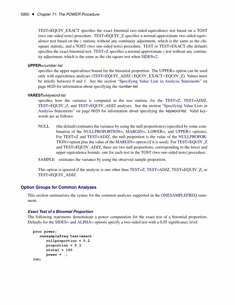
This section summarizes the syntax for the common analyses supported in the ONESAMPLEFREQ state-ment.
Exact Test of a Binomial ProportionThe following statements demonstrate a power computation for the exact test of a binomial proportion.Defaults for the SIDES= and ALPHA= options specify a two-sided test with a 0.05 significance level.
proc power;onesamplefreq test=exact
nullproportion = 0.2proportion = 0.3ntotal = 100power = .;
run;
ONESAMPLEFREQ Statement F 5951
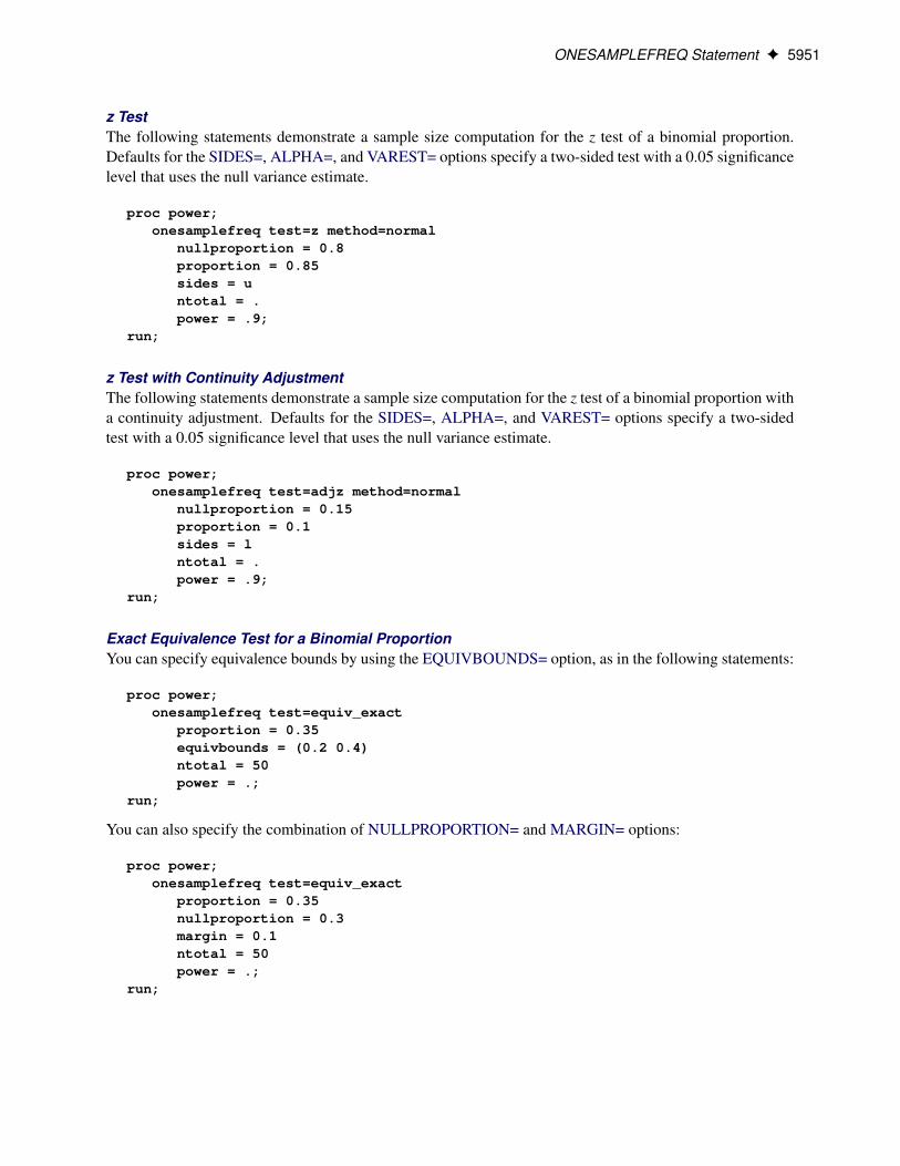
z TestThe following statements demonstrate a sample size computation for the z test of a binomial proportion.Defaults for the SIDES=, ALPHA=, and VAREST= options specify a two-sided test with a 0.05 significancelevel that uses the null variance estimate.
proc power;onesamplefreq test=z method=normal
nullproportion = 0.8proportion = 0.85sides = untotal = .power = .9;
run;
z Test with Continuity AdjustmentThe following statements demonstrate a sample size computation for the z test of a binomial proportion witha continuity adjustment. Defaults for the SIDES=, ALPHA=, and VAREST= options specify a two-sidedtest with a 0.05 significance level that uses the null variance estimate.
proc power;onesamplefreq test=adjz method=normal
nullproportion = 0.15proportion = 0.1sides = lntotal = .power = .9;
run;
Exact Equivalence Test for a Binomial ProportionYou can specify equivalence bounds by using the EQUIVBOUNDS= option, as in the following statements:
proc power;onesamplefreq test=equiv_exact
proportion = 0.35equivbounds = (0.2 0.4)ntotal = 50power = .;
run;
You can also specify the combination of NULLPROPORTION= and MARGIN= options:
proc power;onesamplefreq test=equiv_exact
proportion = 0.35nullproportion = 0.3margin = 0.1ntotal = 50power = .;
run;

5952 F Chapter 71: The POWER Procedure
Finally, you can specify the combination of LOWER= and UPPER= options:
proc power;onesamplefreq test=equiv_exact
proportion = 0.35lower = 0.2upper = 0.4ntotal = 50power = .;
run;
Note that the three preceding analyses are identical.
Exact Noninferiority Test for a Binomial ProportionA noninferiority test corresponds to an upper one-sided test with a negative-valued margin, as demonstratedin the following statements:
proc power;onesamplefreq test=exact
sides = Uproportion = 0.15nullproportion = 0.1margin = -0.02ntotal = 130power = .;
run;
Exact Superiority Test for a Binomial ProportionA superiority test corresponds to an upper one-sided test with a positive-valued margin, as demonstrated inthe following statements:
proc power;onesamplefreq test=exact
sides = Uproportion = 0.15nullproportion = 0.1margin = 0.02ntotal = 130power = .;
run;
Confidence Interval PrecisionThe following statements performs a confidence interval precision analysis for the Wilson score-based con-fidence interval for a binomial proportion. The default value of the ALPHA= option specifies a confidencelevel of 0.95.
proc power;onesamplefreq ci=wilson
halfwidth = 0.1proportion = 0.3ntotal = 70probwidth = .;
run;
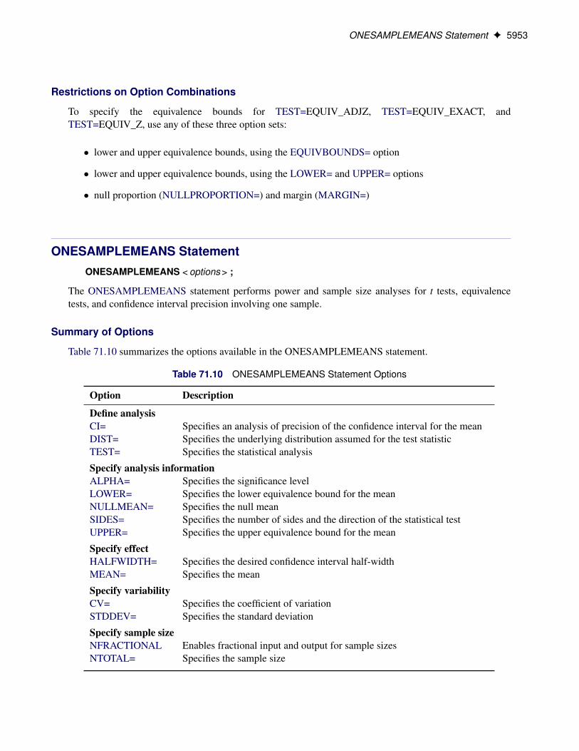
ONESAMPLEMEANS Statement F 5953
Restrictions on Option Combinations
To specify the equivalence bounds for TEST=EQUIV_ADJZ, TEST=EQUIV_EXACT, andTEST=EQUIV_Z, use any of these three option sets:
� lower and upper equivalence bounds, using the EQUIVBOUNDS= option
� lower and upper equivalence bounds, using the LOWER= and UPPER= options
� null proportion (NULLPROPORTION=) and margin (MARGIN=)
ONESAMPLEMEANS StatementONESAMPLEMEANS < options > ;
The ONESAMPLEMEANS statement performs power and sample size analyses for t tests, equivalencetests, and confidence interval precision involving one sample.
Summary of Options
Table 71.10 summarizes the options available in the ONESAMPLEMEANS statement.
Table 71.10 ONESAMPLEMEANS Statement Options
Option Description
Define analysisCI= Specifies an analysis of precision of the confidence interval for the meanDIST= Specifies the underlying distribution assumed for the test statisticTEST= Specifies the statistical analysis
Specify analysis informationALPHA= Specifies the significance levelLOWER= Specifies the lower equivalence bound for the meanNULLMEAN= Specifies the null meanSIDES= Specifies the number of sides and the direction of the statistical testUPPER= Specifies the upper equivalence bound for the mean
Specify effectHALFWIDTH= Specifies the desired confidence interval half-widthMEAN= Specifies the mean
Specify variabilityCV= Specifies the coefficient of variationSTDDEV= Specifies the standard deviation
Specify sample sizeNFRACTIONAL Enables fractional input and output for sample sizesNTOTAL= Specifies the sample size

5954 F Chapter 71: The POWER Procedure
Table 71.10 continued
Option Description
Specify power and related probabilitiesPOWER= Specifies the desired power of the testPROBTYPE= Specifies the type of probability for the PROBWIDTH= optionPROBWIDTH= Specifies the probability of obtaining a confidence interval half-width less
than or equal to the value specified by HALFWIDTH=
Control ordering in outputOUTPUTORDER= Controls the output order of parameters
Table 71.11 summarizes the valid result parameters for different analyses in the ONESAMPLEMEANSstatement.
Table 71.11 Summary of Result Parameters in the ONESAMPLEMEANS Statement
Analyses Solve For Syntax
TEST=T DIST=NORMAL Power POWER=.Sample size NTOTAL=.Alpha ALPHA=.Mean MEAN=.Standard Deviation STDDEV=.
TEST=T DIST=LOGNORMAL Power POWER=.Sample size NTOTAL=.
TEST=EQUIV Power POWER=.Sample size NTOTAL=.
CI=T Prob(width) PROBWIDTH=.Sample size NTOTAL=.
Dictionary of Options
ALPHA=number-listspecifies the level of significance of the statistical test or requests a solution for alpha with a missingvalue (ALPHA=.). The default is 0.05, corresponding to the usual 0.05 � 100% = 5% level of signifi-cance. If the CI= and SIDES=1 options are used, then the value must be less than 0.5. See the section“Specifying Value Lists in Analysis Statements” on page 6020 for information about specifying thenumber-list.
CICI=T
specifies an analysis of precision of the confidence interval for the mean. Instead of power, therelevant probability for this analysis is the probability of achieving a desired precision. Specifically,it is the probability that the half-width of the confidence interval will be at most the value specifiedby the HALFWIDTH= option. If neither the CI= option nor the TEST= option is used, the default isTEST=T.
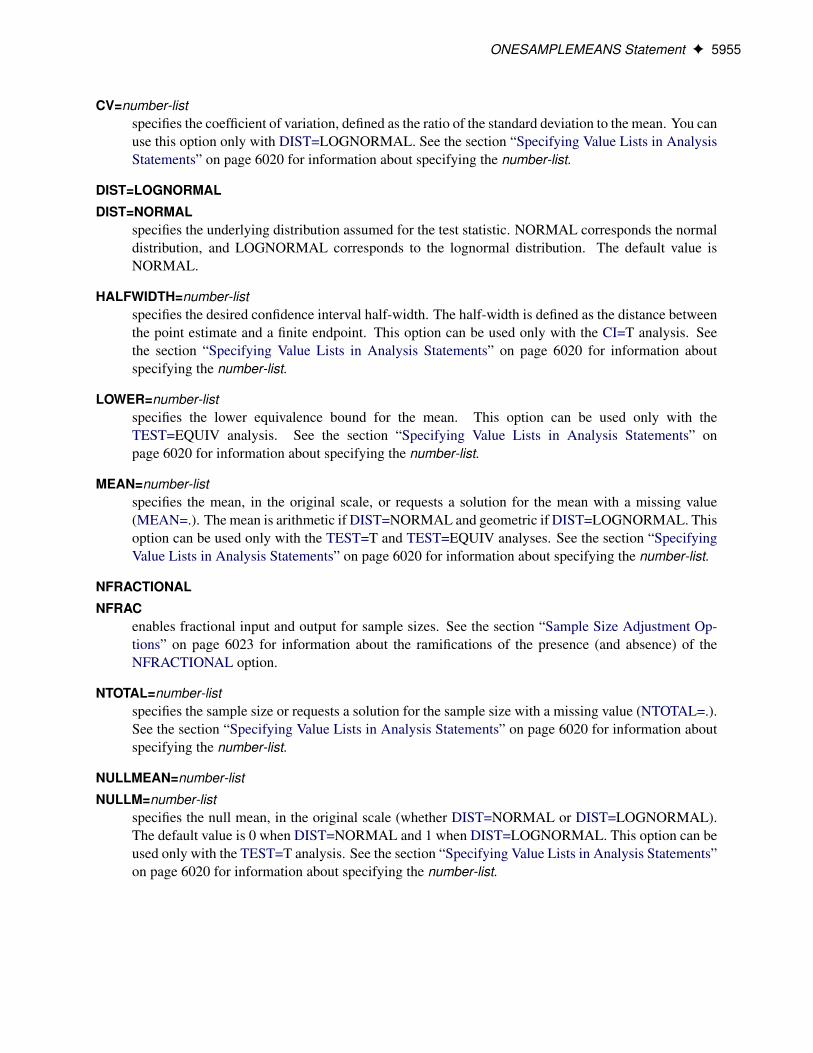
ONESAMPLEMEANS Statement F 5955
CV=number-listspecifies the coefficient of variation, defined as the ratio of the standard deviation to the mean. You canuse this option only with DIST=LOGNORMAL. See the section “Specifying Value Lists in AnalysisStatements” on page 6020 for information about specifying the number-list.
DIST=LOGNORMAL
DIST=NORMALspecifies the underlying distribution assumed for the test statistic. NORMAL corresponds the normaldistribution, and LOGNORMAL corresponds to the lognormal distribution. The default value isNORMAL.
HALFWIDTH=number-listspecifies the desired confidence interval half-width. The half-width is defined as the distance betweenthe point estimate and a finite endpoint. This option can be used only with the CI=T analysis. Seethe section “Specifying Value Lists in Analysis Statements” on page 6020 for information aboutspecifying the number-list.
LOWER=number-listspecifies the lower equivalence bound for the mean. This option can be used only with theTEST=EQUIV analysis. See the section “Specifying Value Lists in Analysis Statements” onpage 6020 for information about specifying the number-list.
MEAN=number-listspecifies the mean, in the original scale, or requests a solution for the mean with a missing value(MEAN=.). The mean is arithmetic if DIST=NORMAL and geometric if DIST=LOGNORMAL. Thisoption can be used only with the TEST=T and TEST=EQUIV analyses. See the section “SpecifyingValue Lists in Analysis Statements” on page 6020 for information about specifying the number-list.
NFRACTIONAL
NFRACenables fractional input and output for sample sizes. See the section “Sample Size Adjustment Op-tions” on page 6023 for information about the ramifications of the presence (and absence) of theNFRACTIONAL option.
NTOTAL=number-listspecifies the sample size or requests a solution for the sample size with a missing value (NTOTAL=.).See the section “Specifying Value Lists in Analysis Statements” on page 6020 for information aboutspecifying the number-list.
NULLMEAN=number-list
NULLM=number-listspecifies the null mean, in the original scale (whether DIST=NORMAL or DIST=LOGNORMAL).The default value is 0 when DIST=NORMAL and 1 when DIST=LOGNORMAL. This option can beused only with the TEST=T analysis. See the section “Specifying Value Lists in Analysis Statements”on page 6020 for information about specifying the number-list.

5956 F Chapter 71: The POWER Procedure
OUTPUTORDER=INTERNAL
OUTPUTORDER=REVERSE
OUTPUTORDER=SYNTAXcontrols how the input and default analysis parameters are ordered in the output. OUT-PUTORDER=INTERNAL (the default) arranges the parameters in the output according to thefollowing order of their corresponding options:
� SIDES=� NULLMEAN=� LOWER=� UPPER=� ALPHA=� MEAN=� HALFWIDTH=� STDDEV=� CV=� NTOTAL=� POWER=� PROBTYPE=� PROBWIDTH=
The OUTPUTORDER=SYNTAX option arranges the parameters in the output in the same orderin which their corresponding options are specified in the ONESAMPLEMEANS statement. TheOUTPUTORDER=REVERSE option arranges the parameters in the output in the reverse of the orderin which their corresponding options are specified in the ONESAMPLEMEANS statement.
POWER=number-listspecifies the desired power of the test or requests a solution for the power with a missing value(POWER=.). The power is expressed as a probability, a number between 0 and 1, rather than asa percentage. This option can be used only with the TEST=T and TEST=EQUIV analyses. Seethe section “Specifying Value Lists in Analysis Statements” on page 6020 for information aboutspecifying the number-list.
PROBTYPE=keyword-listspecifies the type of probability for the PROBWIDTH= option. A value of CONDITIONAL (thedefault) indicates the conditional probability that the confidence interval half-width is at most thevalue specified by the HALFWIDTH= option, given that the true mean is captured by the confidenceinterval. A value of UNCONDITIONAL indicates the unconditional probability that the confidenceinterval half-width is at most the value specified by the HALFWIDTH= option. You can use thealias GIVENVALIDITY for CONDITIONAL. The PROBTYPE= option can be used only with theCI=T analysis. See the section “Specifying Value Lists in Analysis Statements” on page 6020 forinformation about specifying the keyword-list.
CONDITIONAL width probability conditional on interval containing the mean
UNCONDITIONAL unconditional width probability

ONESAMPLEMEANS Statement F 5957
PROBWIDTH=number-listspecifies the desired probability of obtaining a confidence interval half-width less than or equal to thevalue specified by the HALFWIDTH= option. A missing value (PROBWIDTH=.) requests a solutionfor this probability. The type of probability is controlled with the PROBTYPE= option. Values areexpressed as probabilities (for example, 0.9) rather than percentages. This option can be used onlywith the CI=T analysis. See the section “Specifying Value Lists in Analysis Statements” on page 6020for information about specifying the number-list.
SIDES=keyword-listspecifies the number of sides (or tails) and the direction of the statistical test or confidence interval.See the section “Specifying Value Lists in Analysis Statements” on page 6020 for information aboutspecifying the keyword-list. Valid keywords and their interpretation for the TEST= analyses are asfollows:
1 one-sided with alternative hypothesis in same direction as effect
2 two-sided
U upper one-sided with alternative greater than null value
L lower one-sided with alternative less than null value
For confidence intervals, SIDES=U refers to an interval between the lower confidence limit and in-finity, and SIDES=L refers to an interval between minus infinity and the upper confidence limit. Forboth of these cases and SIDES=1, the confidence interval computations are equivalent. The SIDES=option can be used only with the TEST=T and CI=T analyses. The default value is 2.
STDDEV=number-list
STD=number-listspecifies the standard deviation, or requests a solution for the standard deviation with a missing value(STDDEV=.). You can use this option only with DIST=NORMAL. See the section “Specifying ValueLists in Analysis Statements” on page 6020 for information about specifying the number-list.
TEST
TEST=EQUIV
TEST=Tspecifies the statistical analysis. TEST=EQUIV specifies an equivalence test of the mean by using atwo one-sided tests (TOST) analysis (Schuirmann 1987). TEST or TEST=T (the default) specifies a ttest on the mean. If neither the TEST= option nor the CI= option is used, the default is TEST=T.
UPPER=number-listspecifies the upper equivalence bound for the mean, in the original scale (whether DIST=NORMALor DIST=LOGNORMAL). This option can be used only with the TEST=EQUIV analysis. See thesection “Specifying Value Lists in Analysis Statements” on page 6020 for information about specify-ing the number-list.
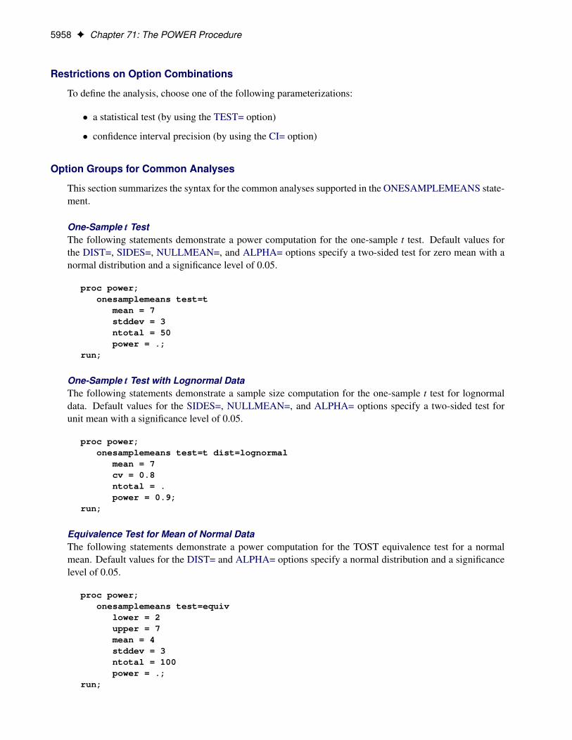
5958 F Chapter 71: The POWER Procedure
Restrictions on Option Combinations
To define the analysis, choose one of the following parameterizations:
� a statistical test (by using the TEST= option)
� confidence interval precision (by using the CI= option)
Option Groups for Common Analyses
This section summarizes the syntax for the common analyses supported in the ONESAMPLEMEANS state-ment.
One-Sample t TestThe following statements demonstrate a power computation for the one-sample t test. Default values forthe DIST=, SIDES=, NULLMEAN=, and ALPHA= options specify a two-sided test for zero mean with anormal distribution and a significance level of 0.05.
proc power;onesamplemeans test=t
mean = 7stddev = 3ntotal = 50power = .;
run;
One-Sample t Test with Lognormal DataThe following statements demonstrate a sample size computation for the one-sample t test for lognormaldata. Default values for the SIDES=, NULLMEAN=, and ALPHA= options specify a two-sided test forunit mean with a significance level of 0.05.
proc power;onesamplemeans test=t dist=lognormal
mean = 7cv = 0.8ntotal = .power = 0.9;
run;
Equivalence Test for Mean of Normal DataThe following statements demonstrate a power computation for the TOST equivalence test for a normalmean. Default values for the DIST= and ALPHA= options specify a normal distribution and a significancelevel of 0.05.
proc power;onesamplemeans test=equiv
lower = 2upper = 7mean = 4stddev = 3ntotal = 100power = .;
run;
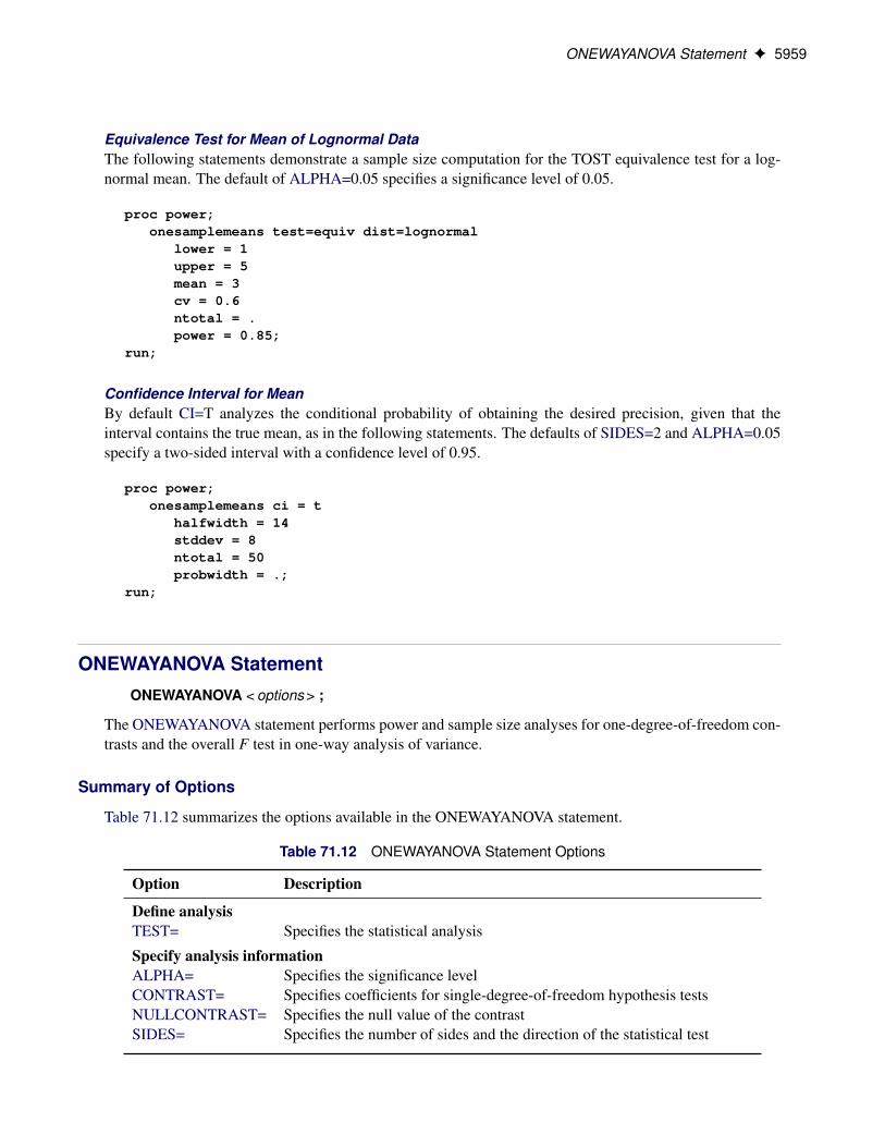
ONEWAYANOVA Statement F 5959
Equivalence Test for Mean of Lognormal DataThe following statements demonstrate a sample size computation for the TOST equivalence test for a log-normal mean. The default of ALPHA=0.05 specifies a significance level of 0.05.
proc power;onesamplemeans test=equiv dist=lognormal
lower = 1upper = 5mean = 3cv = 0.6ntotal = .power = 0.85;
run;
Confidence Interval for MeanBy default CI=T analyzes the conditional probability of obtaining the desired precision, given that theinterval contains the true mean, as in the following statements. The defaults of SIDES=2 and ALPHA=0.05specify a two-sided interval with a confidence level of 0.95.
proc power;onesamplemeans ci = t
halfwidth = 14stddev = 8ntotal = 50probwidth = .;
run;
ONEWAYANOVA StatementONEWAYANOVA < options > ;
The ONEWAYANOVA statement performs power and sample size analyses for one-degree-of-freedom con-trasts and the overall F test in one-way analysis of variance.
Summary of Options
Table 71.12 summarizes the options available in the ONEWAYANOVA statement.
Table 71.12 ONEWAYANOVA Statement Options
Option Description
Define analysisTEST= Specifies the statistical analysis
Specify analysis informationALPHA= Specifies the significance levelCONTRAST= Specifies coefficients for single-degree-of-freedom hypothesis testsNULLCONTRAST= Specifies the null value of the contrastSIDES= Specifies the number of sides and the direction of the statistical test
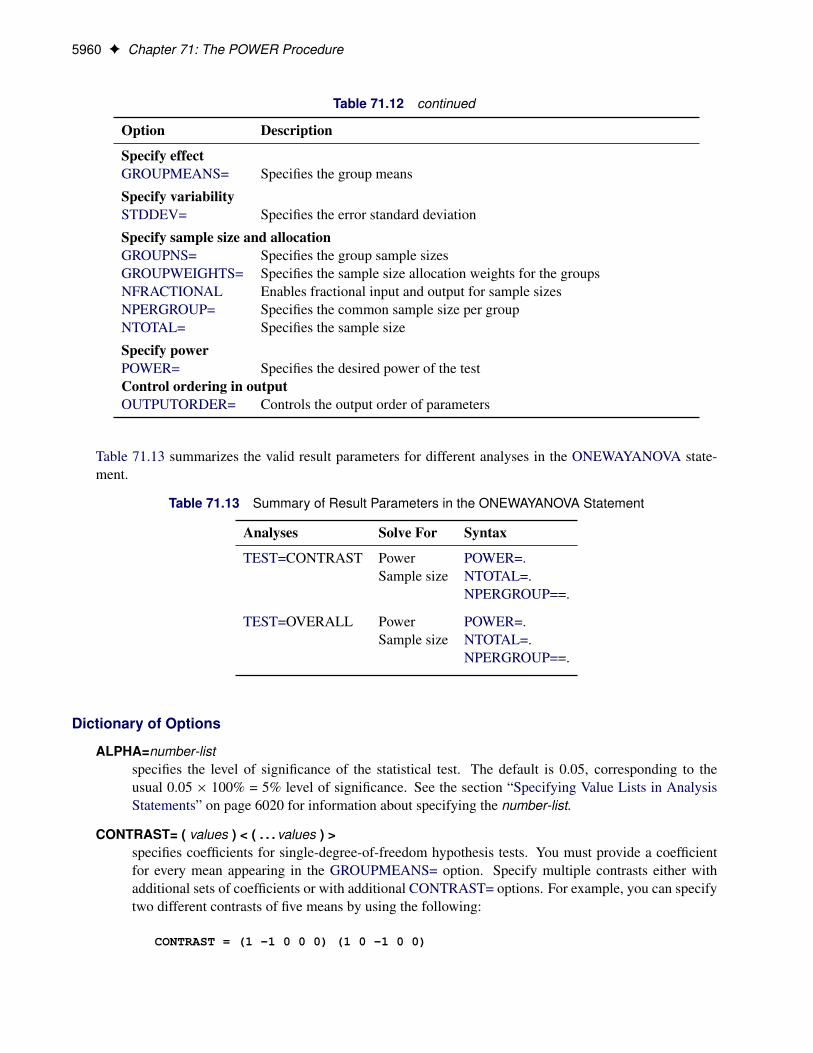
5960 F Chapter 71: The POWER Procedure
Table 71.12 continued
Option Description
Specify effectGROUPMEANS= Specifies the group means
Specify variabilitySTDDEV= Specifies the error standard deviation
Specify sample size and allocationGROUPNS= Specifies the group sample sizesGROUPWEIGHTS= Specifies the sample size allocation weights for the groupsNFRACTIONAL Enables fractional input and output for sample sizesNPERGROUP= Specifies the common sample size per groupNTOTAL= Specifies the sample size
Specify powerPOWER= Specifies the desired power of the testControl ordering in outputOUTPUTORDER= Controls the output order of parameters
Table 71.13 summarizes the valid result parameters for different analyses in the ONEWAYANOVA state-ment.
Table 71.13 Summary of Result Parameters in the ONEWAYANOVA Statement
Analyses Solve For Syntax
TEST=CONTRAST Power POWER=.Sample size NTOTAL=.
NPERGROUP==.
TEST=OVERALL Power POWER=.Sample size NTOTAL=.
NPERGROUP==.
Dictionary of Options
ALPHA=number-listspecifies the level of significance of the statistical test. The default is 0.05, corresponding to theusual 0.05 � 100% = 5% level of significance. See the section “Specifying Value Lists in AnalysisStatements” on page 6020 for information about specifying the number-list.
CONTRAST= ( values ) < ( . . . values ) >specifies coefficients for single-degree-of-freedom hypothesis tests. You must provide a coefficientfor every mean appearing in the GROUPMEANS= option. Specify multiple contrasts either withadditional sets of coefficients or with additional CONTRAST= options. For example, you can specifytwo different contrasts of five means by using the following:
CONTRAST = (1 -1 0 0 0) (1 0 -1 0 0)

ONEWAYANOVA Statement F 5961
GROUPMEANS=grouped-number-list
GMEANS=grouped-number-listspecifies the group means. This option is used to implicitly set the number of groups. See the section“Specifying Value Lists in Analysis Statements” on page 6020 for information about specifying thegrouped-number-list.
GROUPNS=grouped-number-list
GNS=grouped-number-listspecifies the group sample sizes. The number of groups represented must be the same as withthe GROUPMEANS= option. See the section “Specifying Value Lists in Analysis Statements” onpage 6020 for information about specifying the grouped-number-list.
GROUPWEIGHTS=grouped-number-list
GWEIGHTS=grouped-number-listspecifies the sample size allocation weights for the groups. This option controls how the total samplesize is divided between the groups. Each set of values across all groups represents relative allocationweights. Additionally, if the NFRACTIONAL option is not used, the total sample size is restrictedto be equal to a multiple of the sum of the group weights (so that the resulting design has an integersample size for each group while adhering exactly to the group allocation weights). The number ofgroups represented must be the same as with the GROUPMEANS= option. Values must be integersunless the NFRACTIONAL option is used. The default value is 1 for each group, amounting to abalanced design. See the section “Specifying Value Lists in Analysis Statements” on page 6020 forinformation about specifying the grouped-number-list.
NFRACTIONAL
NFRACenables fractional input and output for sample sizes. See the section “Sample Size Adjustment Op-tions” on page 6023 for information about the ramifications of the presence (and absence) of theNFRACTIONAL option.
NPERGROUP=number-list
NPERG=number-listspecifies the common sample size per group or requests a solution for the common sample size pergroup with a missing value (NPERGROUP==.). Use of this option implicitly specifies a balanceddesign. See the section “Specifying Value Lists in Analysis Statements” on page 6020 for informationabout specifying the number-list.
NTOTAL=number-listspecifies the sample size or requests a solution for the sample size with a missing value (NTOTAL=.).See the section “Specifying Value Lists in Analysis Statements” on page 6020 for information aboutspecifying the number-list.
NULLCONTRAST=number-list
NULLC=number-listspecifies the null value of the contrast. The default value is 0. This option can be used only withthe TEST=CONTRAST analysis. See the section “Specifying Value Lists in Analysis Statements” onpage 6020 for information about specifying the number-list.

5962 F Chapter 71: The POWER Procedure
OUTPUTORDER=INTERNAL
OUTPUTORDER=REVERSE
OUTPUTORDER=SYNTAXcontrols how the input and default analysis parameters are ordered in the output. OUT-PUTORDER=INTERNAL (the default) arranges the parameters in the output according to thefollowing order of their corresponding options:
� CONTRAST=� SIDES=� NULLCONTRAST=� ALPHA=� GROUPMEANS=� STDDEV=� GROUPWEIGHTS=� NTOTAL=� NPERGROUP==� GROUPNS=� POWER=
The OUTPUTORDER=SYNTAX option arranges the parameters in the output in the same orderin which their corresponding options are specified in the ONEWAYANOVA statement. The OUT-PUTORDER=REVERSE option arranges the parameters in the output in the reverse of the order inwhich their corresponding options are specified in the ONEWAYANOVA statement.
POWER=number-listspecifies the desired power of the test or requests a solution for the power with a missing value(POWER=.). The power is expressed as a probability, a number between 0 and 1, rather than asa percentage. See the section “Specifying Value Lists in Analysis Statements” on page 6020 forinformation about specifying the number-list.
SIDES=keyword-listspecifies the number of sides (or tails) and the direction of the statistical test. See the section “Specify-ing Value Lists in Analysis Statements” on page 6020 for information about specifying the keyword-list. Valid keywords are as follows:
1 one-sided with alternative hypothesis in same direction as effect
2 two-sided
U upper one-sided with alternative greater than null value
L lower one-sided with alternative less than null value
This option can be used only with the TEST=CONTRAST analysis. The default value is 2.
STDDEV=number-list
STD=number-listspecifies the error standard deviation. See the section “Specifying Value Lists in Analysis Statements”on page 6020 for information about specifying the number-list.

ONEWAYANOVA Statement F 5963
TEST=CONTRAST
TEST=OVERALLspecifies the statistical analysis. TEST=CONTRAST specifies a one-degree-of-freedom test of a con-trast of means. The test is the usual F test for the two-sided case and the usual t test for the one-sided case. TEST=OVERALL specifies the overall F test of equality of all means. The default isTEST=CONTRAST if the CONTRAST= option is used, and TEST=OVERALL otherwise.
Restrictions on Option Combinations
To specify the sample size and allocation, choose one of the following parameterizations:
� sample size per group in a balanced design (by using the NPERGROUP== option)
� total sample size and allocation weights (by using the NTOTAL= and GROUPWEIGHTS= options)
� individual group sample sizes (by using the GROUPNS= option)
Option Groups for Common Analyses
This section summarizes the syntax for the common analyses supported in the ONEWAYANOVA statement.
One-Degree-of-Freedom ContrastYou can use the NPERGROUP== option in a balanced design, as in the following statements. Default valuesfor the SIDES=, NULLCONTRAST=, and ALPHA= options specify a two-sided test for a contrast valueof 0 with a significance level of 0.05.
proc power;onewayanova test=contrast
contrast = (1 0 -1)groupmeans = 3 | 7 | 8stddev = 4npergroup = 50power = .;
run;
You can also specify an unbalanced design with the NTOTAL= and GROUPWEIGHTS= options:
proc power;onewayanova test=contrast
contrast = (1 0 -1)groupmeans = 3 | 7 | 8stddev = 4groupweights = (1 2 2)ntotal = .power = 0.9;
run;

5964 F Chapter 71: The POWER Procedure
Another way to specify the sample sizes is with the GROUPNS= option:
proc power;onewayanova test=contrast
contrast = (1 0 -1)groupmeans = 3 | 7 | 8stddev = 4groupns = (20 40 40)power = .;
run;
Overall F TestThe following statements demonstrate a power computation for the overall F test in a one-way ANOVA.The default of ALPHA=0.05 specifies a significance level of 0.05.
proc power;onewayanova test=overall
groupmeans = 3 | 7 | 8stddev = 4npergroup = 50power = .;
run;
PAIREDFREQ StatementPAIREDFREQ < options > ;
The PAIREDFREQ statement performs power and sample size analyses for McNemar’s test for pairedproportions.
Summary of Options
Table 71.14 summarizes the options available in the PAIREDFREQ statement.
Table 71.14 PAIREDFREQ Statement Options
Option Description
Define analysisDIST= Specifies the underlying distribution assumed for the test statisticTEST= Specifies the statistical analysis
Specify analysis informationALPHA= Specifies the significance levelNULLDISCPROPRATIO= Specifies the null value of the ratio of discordant proportionsSIDES= Specifies the number of sides and the direction of the statistical test or
confidence interval
Specify effectsCORR= Specifies the correlation � between members of a pairDISCPROPDIFF= Specifies the discordant proportion difference p01 � p10DISCPROPORTIONS= Specifies the two discordant proportions, p10 and p01

PAIREDFREQ Statement F 5965
Table 71.14 continued
Option Description
DISCPROPRATIO= Specifies the ratio p01=p10ODDSRATIO= Specifies the odds ratio Œp�1=.1 � p�1/� = Œp1�=.1 � p1�/�PAIREDPROPORTIONS= Specifies the two paired proportions, p1� and p�1PROPORTIONDIFF= Specifies the proportion difference p�1 � p1�REFPROPORTION= Specifies either the reference first proportion p1� or the reference discor-
dant proportion p10RELATIVERISK= Specifies the relative risk p�1=p1�TOTALPROPDISC= Specifies the discordant proportion sum, p10 C p01Specify sample sizeNFRACTIONAL Enables fractional input and output for sample sizesNPAIRS= Specifies the total number of proportion pairs
Specify powerPOWER= Specifies the desired power of the test
Choose computational methodMETHOD= Specifies the computational method
Control ordering in outputOUTPUTORDER= Controls the output order of parameters
Table 71.15 summarizes the valid result parameters in the PAIREDFREQ statement.
Table 71.15 Summary of Result Parameters in the PAIREDFREQ Statement
Analyses Solve For Syntax
TEST=MCNEMAR METHOD=CONNOR Power POWER=.Sample size NPAIRS=.
TEST=MCNEMAR METHOD=EXACT Power POWER=.
TEST=MCNEMAR METHOD=MIETTINEN Power POWER=.Sample size NPAIRS=.
Dictionary of Options
ALPHA=number-listspecifies the level of significance of the statistical test. The default is 0.05, corresponding to theusual 0.05 � 100% = 5% level of significance. See the section “Specifying Value Lists in AnalysisStatements” on page 6020 for information about specifying the number-list.
CORR=number-listspecifies the correlation � between members of a pair. See the section “Specifying Value Lists inAnalysis Statements” on page 6020 for information about specifying the number-list.
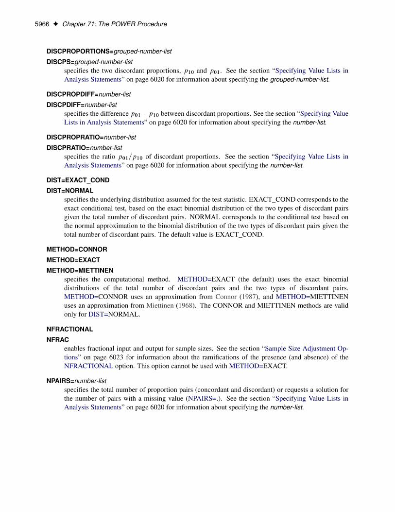
5966 F Chapter 71: The POWER Procedure
DISCPROPORTIONS=grouped-number-list
DISCPS=grouped-number-listspecifies the two discordant proportions, p10 and p01. See the section “Specifying Value Lists inAnalysis Statements” on page 6020 for information about specifying the grouped-number-list.
DISCPROPDIFF=number-list
DISCPDIFF=number-listspecifies the difference p01�p10 between discordant proportions. See the section “Specifying ValueLists in Analysis Statements” on page 6020 for information about specifying the number-list.
DISCPROPRATIO=number-list
DISCPRATIO=number-listspecifies the ratio p01=p10 of discordant proportions. See the section “Specifying Value Lists inAnalysis Statements” on page 6020 for information about specifying the number-list.
DIST=EXACT_COND
DIST=NORMALspecifies the underlying distribution assumed for the test statistic. EXACT_COND corresponds to theexact conditional test, based on the exact binomial distribution of the two types of discordant pairsgiven the total number of discordant pairs. NORMAL corresponds to the conditional test based onthe normal approximation to the binomial distribution of the two types of discordant pairs given thetotal number of discordant pairs. The default value is EXACT_COND.
METHOD=CONNOR
METHOD=EXACT
METHOD=MIETTINENspecifies the computational method. METHOD=EXACT (the default) uses the exact binomialdistributions of the total number of discordant pairs and the two types of discordant pairs.METHOD=CONNOR uses an approximation from Connor (1987), and METHOD=MIETTINENuses an approximation from Miettinen (1968). The CONNOR and MIETTINEN methods are validonly for DIST=NORMAL.
NFRACTIONAL
NFRACenables fractional input and output for sample sizes. See the section “Sample Size Adjustment Op-tions” on page 6023 for information about the ramifications of the presence (and absence) of theNFRACTIONAL option. This option cannot be used with METHOD=EXACT.
NPAIRS=number-listspecifies the total number of proportion pairs (concordant and discordant) or requests a solution forthe number of pairs with a missing value (NPAIRS=.). See the section “Specifying Value Lists inAnalysis Statements” on page 6020 for information about specifying the number-list.

PAIREDFREQ Statement F 5967
NULLDISCPROPRATIO=number-list
NULLDISCPRATIO=number-list
NULLRATIO=number-list
NULLR=number-listspecifies the null value of the ratio of discordant proportions. The default value is 1. See the section“Specifying Value Lists in Analysis Statements” on page 6020 for information about specifying thenumber-list.
ODDSRATIO=number-list
OR=number-listspecifies the odds ratio Œp�1=.1 � p�1/� = Œp1�=.1 � p1�/�. See the section “Specifying Value Lists inAnalysis Statements” on page 6020 for information about specifying the number-list.
OUTPUTORDER=INTERNAL
OUTPUTORDER=REVERSE
OUTPUTORDER=SYNTAXcontrols how the input and default analysis parameters are ordered in the output. OUT-PUTORDER=INTERNAL (the default) arranges the parameters in the output according to thefollowing order of their corresponding options:
� SIDES=� NULLDISCPROPRATIO=� ALPHA=� PAIREDPROPORTIONS=� PROPORTIONDIFF=� ODDSRATIO=� RELATIVERISK=� CORR=� DISCPROPORTIONS=� DISCPROPDIFF=� TOTALPROPDISC=� REFPROPORTION=� DISCPROPRATIO=� NPAIRS=� POWER=
The OUTPUTORDER=SYNTAX option arranges the parameters in the output in the same orderin which their corresponding options are specified in the PAIREDFREQ statement. The OUT-PUTORDER=REVERSE option arranges the parameters in the output in the reverse of the orderin which their corresponding options are specified in the PAIREDFREQ statement.

5968 F Chapter 71: The POWER Procedure
PAIREDPROPORTIONS=grouped-number-list
PPROPORTIONS=grouped-number-list
PAIREDPS=grouped-number-list
PPS=grouped-number-listspecifies the two paired proportions, p1� and p�1. See the section “Specifying Value Lists in AnalysisStatements” on page 6020 for information about specifying the grouped-number-list.
POWER=number-listspecifies the desired power of the test or requests a solution for the power with a missing value(POWER=.). The power is expressed as a probability, a number between 0 and 1, rather than asa percentage. See the section “Specifying Value Lists in Analysis Statements” on page 6020 forinformation about specifying the number-list.
PROPORTIONDIFF=number-list
PDIFF=number-listspecifies the proportion difference p�1 � p1�. See the section “Specifying Value Lists in AnalysisStatements” on page 6020 for information about specifying the number-list.
REFPROPORTION=number-list
REFP=number-listspecifies either the reference first proportion p1� (when used in conjunction with the PROPORTION-DIFF=, ODDSRATIO=, or RELATIVERISK= option) or the reference discordant proportion p10(when used in conjunction with the DISCPROPDIFF= or DISCPROPRATIO= option). See the sec-tion “Specifying Value Lists in Analysis Statements” on page 6020 for information about specifyingthe number-list.
RELATIVERISK=number-list
RR=number-listspecifies the relative risk p�1=p1�. See the section “Specifying Value Lists in Analysis Statements” onpage 6020 for information about specifying the number-list.
SIDES=keyword-listspecifies the number of sides (or tails) and the direction of the statistical test or confidence interval.See the section “Specifying Value Lists in Analysis Statements” on page 6020 for information aboutspecifying the keyword-list. Valid keywords and their interpretation are as follows:
1 one-sided with alternative hypothesis in same direction as effect
2 two-sided
U upper one-sided with alternative greater than null value
L lower one-sided with alternative less than null value
If the effect size is zero, then SIDES=1 is not permitted; instead, specify the direction of the testexplicitly in this case with either SIDES=L or SIDES=U. The default value is 2.
TEST=MCNEMARspecifies the McNemar test of paired proportions. This is the default test option.

PAIREDFREQ Statement F 5969
TOTALPROPDISC=number-listTOTALPDISC=number-listPDISC=number-list
specifies the sum of the two discordant proportions, p10 C p01. See the section “Specifying ValueLists in Analysis Statements” on page 6020 for information about specifying the number-list.
Restrictions on Option Combinations
To specify the proportions, choose one of the following parameterizations:
� discordant proportions (using the DISCPROPORTIONS= option)
� difference and sum of discordant proportions (using the DISCPROPDIFF= and TOTAL-PROPDISC=options)
� difference of discordant proportions and reference discordant proportion (using the DISCPROPDIFF=and REFPROPORTION= options)
� ratio of discordant proportions and reference discordant proportion (using the DISCPROPRATIO=and REFPROPORTION= options)
� ratio and sum of discordant proportions (using the DISCPROPRATIO= and TOTAL-PROPDISC=options)
� paired proportions and correlation (using the PAIREDPROPORTIONS= and CORR= options)
� proportion difference, reference proportion, and correlation (using the PROPORTIONDIFF=, REF-PROPORTION=, and CORR= options)
� odds ratio, reference proportion, and correlation (using the ODDSRATIO=, REFPROPORTION=,and CORR= options)
� relative risk, reference proportion, and correlation (using the RELATIVERISK=, REFPROPOR-TION=, and CORR= options)
Option Groups for Common Analyses
This section summarizes the syntax for the common analyses supported in the PAIREDFREQ statement.
McNemar Exact Conditional TestYou can express effects in terms of the individual discordant proportions, as in the following statements.Default values for the TEST=, SIDES=, ALPHA=, and NULLDISCPROPRATIO= options specify a two-sided McNemar test for no effect with a significance level of 0.05.
proc power;pairedfreq dist=exact_cond
discproportions = 0.15 | 0.45npairs = 80power = .;
run;
You can also express effects in terms of the difference and sum of discordant proportions:

5970 F Chapter 71: The POWER Procedure
proc power;pairedfreq dist=exact_cond
discpropdiff = 0.3totalpropdisc = 0.6npairs = 80power = .;
run;
You can also express effects in terms of the difference of discordant proportions and the reference discordantproportion:
proc power;pairedfreq dist=exact_cond
discpropdiff = 0.3refproportion = 0.15npairs = 80power = .;
run;
You can also express effects in terms of the ratio of discordant proportions and the denominator of the ratio:
proc power;pairedfreq dist=exact_cond
discpropratio = 3refproportion = 0.15npairs = 80power = .;
run;
You can also express effects in terms of the ratio and sum of discordant proportions:
proc power;pairedfreq dist=exact_cond
discpropratio = 3totalpropdisc = 0.6npairs = 80power = .;
run;
You can also express effects in terms of the paired proportions and correlation:
proc power;pairedfreq dist=exact_cond
pairedproportions = 0.6 | 0.8corr = 0.4npairs = 45power = .;
run;
You can also express effects in terms of the proportion difference, reference proportion, and correlation:
proc power;pairedfreq dist=exact_cond
proportiondiff = 0.2refproportion = 0.6

PAIREDMEANS Statement F 5971
corr = 0.4npairs = 45power = .;
run;
You can also express effects in terms of the odds ratio, reference proportion, and correlation:
proc power;pairedfreq dist=exact_cond
oddsratio = 2.66667refproportion = 0.6corr = 0.4npairs = 45power = .;
run;
You can also express effects in terms of the relative risk, reference proportion, and correlation:
proc power;pairedfreq dist=exact_cond
relativerisk = 1.33333refproportion = 0.6corr = 0.4npairs = 45power = .;
run;
McNemar Normal Approximation TestThe following statements demonstrate a sample size computation for the normal-approximate McNemartest. The default value for the METHOD= option specifies an exact sample size computation. Default valuesfor the TEST=, SIDES=, ALPHA=, and NULLDISCPROPRATIO= options specify a two-sided McNemartest for no effect with a significance level of 0.05.
proc power;pairedfreq dist=normal method=connor
discproportions = 0.15 | 0.45npairs = .power = .9;
run;
PAIREDMEANS StatementPAIREDMEANS < options > ;
The PAIREDMEANS statement performs power and sample size analyses for t tests, equivalence tests, andconfidence interval precision involving paired samples.
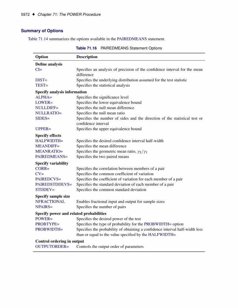
5972 F Chapter 71: The POWER Procedure
Summary of Options
Table 71.14 summarizes the options available in the PAIREDMEANS statement.
Table 71.16 PAIREDMEANS Statement Options
Option Description
Define analysisCI= Specifies an analysis of precision of the confidence interval for the mean
differenceDIST= Specifies the underlying distribution assumed for the test statisticTEST= Specifies the statistical analysis
Specify analysis informationALPHA= Specifies the significance levelLOWER= Specifies the lower equivalence boundNULLDIFF= Specifies the null mean differenceNULLRATIO= Specifies the null mean ratioSIDES= Specifies the number of sides and the direction of the statistical test or
confidence intervalUPPER= Specifies the upper equivalence bound
Specify effectsHALFWIDTH= Specifies the desired confidence interval half-widthMEANDIFF= Specifies the mean differenceMEANRATIO= Specifies the geometric mean ratio, 2= 1PAIREDMEANS= Specifies the two paired means
Specify variabilityCORR= Specifies the correlation between members of a pairCV= Specifies the common coefficient of variationPAIREDCVS= Specifies the coefficient of variation for each member of a pairPAIREDSTDDEVS= Specifies the standard deviation of each member of a pairSTDDEV= Specifies the common standard deviation
Specify sample sizeNFRACTIONAL Enables fractional input and output for sample sizesNPAIRS= Specifies the number of pairs
Specify power and related probabilitiesPOWER= Specifies the desired power of the testPROBTYPE= Specifies the type of probability for the PROBWIDTH= optionPROBWIDTH= Specifies the probability of obtaining a confidence interval half-width less
than or equal to the value specified by the HALFWIDTH=
Control ordering in outputOUTPUTORDER= Controls the output order of parameters

PAIREDMEANS Statement F 5973
Table 71.17 summarizes the valid result parameters for different analyses in the PAIREDMEANS statement.
Table 71.17 Summary of Result Parameters in the PAIREDMEANS Statement
Analyses Solve For Syntax
TEST=DIFF Power POWER=.Sample size NPAIRS=.
TEST=RATIO Power POWER=.Sample size NPAIRS=.
TEST=EQUIV_DIFF Power POWER=.Sample size NPAIRS=.
TEST=EQUIV_RATIO Power POWER=.Sample size NPAIRS=.
CI=DIFF Prob(width) PROBWIDTH=.Sample size NPAIRS=.
Dictionary of Options
ALPHA=number-listspecifies the level of significance of the statistical test. The default is 0.05, corresponding to the usual0.05 � 100% = 5% level of significance. If the CI= and SIDES=1 options are used, then the valuemust be less than 0.5. See the section “Specifying Value Lists in Analysis Statements” on page 6020for information about specifying the number-list.
CI
CI=DIFFspecifies an analysis of precision of the confidence interval for the mean difference. Instead of power,the relevant probability for this analysis is the probability of achieving a desired precision. Specifi-cally, it is the probability that the half-width of the observed confidence interval will be at most thevalue specified by the HALFWIDTH= option. If neither the CI= option nor the TEST= option is used,the default is TEST=DIFF.
CORR=number-listspecifies the correlation between members of a pair. See the section “Specifying Value Lists in Anal-ysis Statements” on page 6020 for information about specifying the number-list.
CV=number-listspecifies the coefficient of variation assumed to be common to both members of a pair. The coefficientof variation is defined as the ratio of the standard deviation to the mean. You can use this optiononly with DIST=LOGNORMAL. See the section “Specifying Value Lists in Analysis Statements” onpage 6020 for information about specifying the number-list.

5974 F Chapter 71: The POWER Procedure
DIST=LOGNORMAL
DIST=NORMALspecifies the underlying distribution assumed for the test statistic. NORMAL corresponds the normaldistribution, and LOGNORMAL corresponds to the lognormal distribution. The default value (alsothe only acceptable value in each case) is NORMAL for TEST=DIFF, TEST=EQUIV_DIFF, andCI=DIFF; and LOGNORMAL for TEST=RATIO and TEST=EQUIV_RATIO.
HALFWIDTH=number-listspecifies the desired confidence interval half-width. The half-width is defined as the distance betweenthe point estimate and a finite endpoint. This option can be used only with the CI=DIFF analysis.See the section “Specifying Value Lists in Analysis Statements” on page 6020 for information aboutspecifying the number-list.
LOWER=number-listspecifies the lower equivalence bound for the mean difference or mean ratio, in the originalscale (whether DIST=NORMAL or DIST=LOGNORMAL). This option can be used only with theTEST=EQUIV_DIFF and TEST=EQUIV_RATIO analyses. See the section “Specifying Value Listsin Analysis Statements” on page 6020 for information about specifying the number-list.
MEANDIFF=number-listspecifies the mean difference, defined as the mean of the difference between the second and first mem-bers of a pair, �2��1. This option can be used only with the TEST=DIFF and TEST=EQUIV_DIFFanalyses. When TEST=EQUIV_DIFF, the mean difference is interpreted as the treatment mean minusthe reference mean. See the section “Specifying Value Lists in Analysis Statements” on page 6020for information about specifying the number-list.
MEANRATIO=number-listspecifies the geometric mean ratio, defined as 2= 1. This option can be used only with theTEST=RATIO and TEST=EQUIV_RATIO analyses. When TEST=EQUIV_RATIO, the mean ra-tio is interpreted as the treatment mean divided by the reference mean. See the section “SpecifyingValue Lists in Analysis Statements” on page 6020 for information about specifying the number-list.
NFRACTIONAL
NFRACenables fractional input and output for sample sizes. See the section “Sample Size Adjustment Op-tions” on page 6023 for information about the ramifications of the presence (and absence) of theNFRACTIONAL option.
NPAIRS=number-listspecifies the number of pairs or requests a solution for the number of pairs with a missing value(NPAIRS=.). See the section “Specifying Value Lists in Analysis Statements” on page 6020 forinformation about specifying the number-list.
NULLDIFF=number-list
NULLD=number-listspecifies the null mean difference. The default value is 0. This option can be used only with theTEST=DIFF analysis. See the section “Specifying Value Lists in Analysis Statements” on page 6020for information about specifying the number-list.

PAIREDMEANS Statement F 5975
NULLRATIO=number-list
NULLR=number-listspecifies the null mean ratio. The default value is 1. This option can be used only with theTEST=RATIO analysis. See the section “Specifying Value Lists in Analysis Statements” onpage 6020 for information about specifying the number-list.
OUTPUTORDER=INTERNAL
OUTPUTORDER=REVERSE
OUTPUTORDER=SYNTAXcontrols how the input and default analysis parameters are ordered in the output. OUT-PUTORDER=INTERNAL (the default) arranges the parameters in the output according to thefollowing order of their corresponding options:
� SIDES=� NULLDIFF=� NULLRATIO=� LOWER=� UPPER=� ALPHA=� PAIREDMEANS=� MEANDIFF=� MEANRATIO=� HALFWIDTH=� STDDEV=� PAIREDSTDDEVS=� CV=� PAIREDCVS=� CORR=� NPAIRS=� POWER=� PROBTYPE=� PROBWIDTH=
The OUTPUTORDER=SYNTAX option arranges the parameters in the output in the same orderin which their corresponding options are specified in the PAIREDMEANS statement. The OUT-PUTORDER=REVERSE option arranges the parameters in the output in the reverse of the order inwhich their corresponding options are specified in the PAIREDMEANS statement.
PAIREDCVS=grouped-number-listspecifies the coefficient of variation for each member of a pair. Unlike the CV= option, the PAIRED-CVS= option supports different values for each member of a pair. Values must be nonnegative (unlessboth are equal to zero, which is permitted). This option can be used only with DIST=LOGNORMAL.See the section “Specifying Value Lists in Analysis Statements” on page 6020 for information aboutspecifying the grouped-number-list.

5976 F Chapter 71: The POWER Procedure
PAIREDMEANS=grouped-number-list
PMEANS=grouped-number-listspecifies the two paired means, in the original scale. The means are arithmetic if DIST=NORMALand geometric if DIST=LOGNORMAL. This option cannot be used with the CI=DIFF analysis.When TEST=EQUIV_DIFF, the means are interpreted as the reference mean (first) and the treat-ment mean (second). See the section “Specifying Value Lists in Analysis Statements” on page 6020for information about specifying the grouped-number-list.
PAIREDSTDDEVS=grouped-number-list
PAIREDSTDS=grouped-number-list
PSTDDEVS=grouped-number-list
PSTDS=grouped-number-listspecifies the standard deviation of each member of a pair. Unlike the STDDEV= option, the PAIRED-STDDEVS= option supports different values for each member of a pair. This option can be used onlywith DIST=NORMAL. See the section “Specifying Value Lists in Analysis Statements” on page 6020for information about specifying the grouped-number-list.
POWER=number-listspecifies the desired power of the test or requests a solution for the power with a missing value(POWER=.). The power is expressed as a probability, a number between 0 and 1, rather than asa percentage. This option cannot be used with the CI=DIFF analysis. See the section “SpecifyingValue Lists in Analysis Statements” on page 6020 for information about specifying the number-list.
PROBTYPE=keyword-listspecifies the type of probability for the PROBWIDTH= option. A value of CONDITIONAL (thedefault) indicates the conditional probability that the confidence interval half-width is at most thevalue specified by the HALFWIDTH= option, given that the true mean difference is captured bythe confidence interval. A value of UNCONDITIONAL indicates the unconditional probability thatthe confidence interval half-width is at most the value specified by the HALFWIDTH= option. youcan use the alias GIVENVALIDITY for CONDITIONAL. The PROBTYPE= option can be usedonly with the CI=DIFF analysis. See the section “Specifying Value Lists in Analysis Statements” onpage 6020 for information about specifying the keyword-list.
CONDITIONAL width probability conditional on interval containing the mean
UNCONDITIONAL unconditional width probability
PROBWIDTH=number-listspecifies the desired probability of obtaining a confidence interval half-width less than or equal to thevalue specified by the HALFWIDTH= option. A missing value (PROBWIDTH=.) requests a solutionfor this probability. The type of probability is controlled with the PROBTYPE= option. Values areexpressed as probabilities (for example, 0.9) rather than percentages. This option can be used onlywith the CI=DIFF analysis. See the section “Specifying Value Lists in Analysis Statements” onpage 6020 for information about specifying the number-list.
SIDES=keyword-listspecifies the number of sides (or tails) and the direction of the statistical test or confidence interval.See the section “Specifying Value Lists in Analysis Statements” on page 6020 for information aboutspecifying the keyword-list. Valid keywords and their interpretation for the TEST= analyses are asfollows:

PAIREDMEANS Statement F 5977
1 one-sided with alternative hypothesis in same direction as effect
2 two-sided
U upper one-sided with alternative greater than null value
L lower one-sided with alternative less than null value
For confidence intervals, SIDES=U refers to an interval between the lower confidence limit and infin-ity, and SIDES=L refers to an interval between minus infinity and the upper confidence limit. For bothof these cases and SIDES=1, the confidence interval computations are equivalent. The SIDES= op-tion cannot be used with the TEST=EQUIV_DIFF and TEST=EQUIV_RATIO analyses. The defaultvalue is 2.
STDDEV=number-listSTD=number-list
specifies the standard deviation assumed to be common to both members of a pair. This option canbe used only with DIST=NORMAL. See the section “Specifying Value Lists in Analysis Statements”on page 6020 for information about specifying the number-list.
TESTTEST=DIFFTEST=EQUIV_DIFFTEST=EQUIV_RATIOTEST=RATIO
specifies the statistical analysis. TEST or TEST=DIFF (the default) specifies a paired t test on themean difference. TEST=EQUIV_DIFF specifies an additive equivalence test of the mean differenceby using a two one-sided tests (TOST) analysis (Schuirmann 1987). TEST=EQUIV_RATIO specifiesa multiplicative equivalence test of the mean ratio by using a TOST analysis. TEST=RATIO specifiesa paired t test on the geometric mean ratio. If neither the TEST= option nor the CI= option is used,the default is TEST=DIFF.
UPPER=number-listspecifies the upper equivalence bound for the mean difference or mean ratio, in the originalscale (whether DIST=NORMAL or DIST=LOGNORMAL). This option can be used only with theTEST=EQUIV_DIFF and TEST=EQUIV_RATIO analyses. See the section “Specifying Value Listsin Analysis Statements” on page 6020 for information about specifying the number-list.
Restrictions on Option Combinations
To define the analysis, choose one of the following parameterizations:
� a statistical test (by using the TEST= option)
� confidence interval precision (by using the CI= option)
To specify the means, choose one of the following parameterizations:
� individual means (by using the PAIREDMEANS= option)
� mean difference (by using the MEANDIFF= option)
� mean ratio (by using the MEANRATIO= option)

5978 F Chapter 71: The POWER Procedure
To specify the coefficient of variation, choose one of the following parameterizations:
� common coefficient of variation (by using the CV= option)
� individual coefficients of variation (by using the PAIREDCVS= option)
To specify the standard deviation, choose one of the following parameterizations:
� common standard deviation (by using the STDDEV= option)
� individual standard deviations (by using the PAIREDSTDDEVS= option)
Option Groups for Common Analyses
This section summarizes the syntax for the common analyses supported in the PAIREDMEANS statement.
Paired t TestYou can express effects in terms of the mean difference and variability in terms of a correlation and commonstandard deviation, as in the following statements. Default values for the DIST=, SIDES=, NULLDIFF=,and ALPHA= options specify a two-sided test for no difference with a normal distribution and a significancelevel of 0.05.
proc power;pairedmeans test=diff
meandiff = 7corr = 0.4stddev = 12npairs = 50power = .;
run;
You can also express effects in terms of individual means and variability in terms of correlation and individ-ual standard deviations:
proc power;pairedmeans test=diff
pairedmeans = 8 | 15corr = 0.4pairedstddevs = (7 12)npairs = .power = 0.9;
run;
Paired t Test of Mean Ratio with Lognormal DataYou can express variability in terms of correlation and a common coefficient of variation, as in the followingstatements. Defaults for the DIST=, SIDES=, NULLRATIO= and ALPHA= options specify a two-sided testof mean ratio = 1 assuming a lognormal distribution and a significance level of 0.05.

PAIREDMEANS Statement F 5979
proc power;pairedmeans test=ratio
meanratio = 7corr = 0.3cv = 1.2npairs = 30power = .;
run;
You can also express variability in terms of correlation and individual coefficients of variation:
proc power;pairedmeans test=ratio
meanratio = 7corr = 0.3pairedcvs = 0.8 | 0.9npairs = 30power = .;
run;
Additive Equivalence Test for Mean Difference with Normal DataThe following statements demonstrate a sample size computation for a TOST equivalence test for a normalmean difference. Default values for the DIST= and ALPHA= options specify a normal distribution and asignificance level of 0.05.
proc power;pairedmeans test=equiv_diff
lower = 2upper = 5meandiff = 4corr = 0.2stddev = 8npairs = .power = 0.9;
run;
Multiplicative Equivalence Test for Mean Ratio with Lognormal DataThe following statements demonstrate a power computation for a TOST equivalence test for a lognormalmean ratio. Default values for the DIST= and ALPHA= options specify a lognormal distribution and asignificance level of 0.05.
proc power;pairedmeans test=equiv_ratio
lower = 3upper = 7meanratio = 5corr = 0.2cv = 1.1npairs = 50power = .;
run;

5980 F Chapter 71: The POWER Procedure
Confidence Interval for Mean DifferenceBy default CI=DIFF analyzes the conditional probability of obtaining the desired precision, given that theinterval contains the true mean difference, as in the following statements. The defaults of SIDES=2 andALPHA=0.05 specify a two-sided interval with a confidence level of 0.95.
proc power;pairedmeans ci = diff
halfwidth = 4corr = 0.35stddev = 8npairs = 30probwidth = .;
run;
PLOT StatementPLOT < plot-options > < / graph-options > ;
The PLOT statement produces a graph or set of graphs for the sample size analysis defined by the previousanalysis statement. The plot-options define the plot characteristics, and the graph-options are SAS/GRAPH-style options. If ODS Graphics is enabled, then the PLOT statement uses ODS Graphics to create graphs.For example:
ods listing style=htmlbluecml;ods graphics on;
proc power;onesamplemeans
mean = 5 10ntotal = 150stddev = 30 50power = .;
plot x=n min=100 max=200;run;
ods graphics off;
Otherwise, traditional graphics are produced. For example:
ods graphics off;
proc power;onesamplemeans
mean = 5 10ntotal = 150stddev = 30 50power = .;
plot x=n min=100 max=200;run;
For more information about enabling and disabling ODS Graphics, see the section “Enabling and DisablingODS Graphics” on page 600 in Chapter 21, “Statistical Graphics Using ODS.”
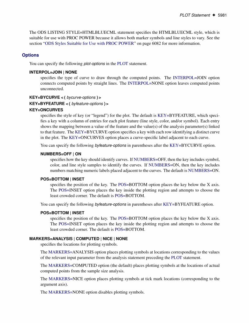
PLOT Statement F 5981
The ODS LISTING STYLE=HTMLBLUECML statement specifies the HTMLBLUECML style, which issuitable for use with PROC POWER because it allows both marker symbols and line styles to vary. See thesection “ODS Styles Suitable for Use with PROC POWER” on page 6082 for more information.
Options
You can specify the following plot-options in the PLOT statement.
INTERPOL=JOIN | NONEspecifies the type of curve to draw through the computed points. The INTERPOL=JOIN optionconnects computed points by straight lines. The INTERPOL=NONE option leaves computed pointsunconnected.
KEY=BYCURVE < ( bycurve-options ) >KEY=BYFEATURE < ( byfeature-options ) >KEY=ONCURVES
specifies the style of key (or “legend”) for the plot. The default is KEY=BYFEATURE, which speci-fies a key with a column of entries for each plot feature (line style, color, and/or symbol). Each entryshows the mapping between a value of the feature and the value(s) of the analysis parameter(s) linkedto that feature. The KEY=BYCURVE option specifies a key with each row identifying a distinct curvein the plot. The KEY=ONCURVES option places a curve-specific label adjacent to each curve.
You can specify the following byfeature-options in parentheses after the KEY=BYCURVE option.
NUMBERS=OFF | ONspecifies how the key should identify curves. If NUMBERS=OFF, then the key includes symbol,color, and line style samples to identify the curves. If NUMBERS=ON, then the key includesnumbers matching numeric labels placed adjacent to the curves. The default is NUMBERS=ON.
POS=BOTTOM | INSETspecifies the position of the key. The POS=BOTTOM option places the key below the X axis.The POS=INSET option places the key inside the plotting region and attempts to choose theleast crowded corner. The default is POS=BOTTOM.
You can specify the following byfeature-options in parentheses after KEY=BYFEATURE option.
POS=BOTTOM | INSETspecifies the position of the key. The POS=BOTTOM option places the key below the X axis.The POS=INSET option places the key inside the plotting region and attempts to choose theleast crowded corner. The default is POS=BOTTOM.
MARKERS=ANALYSIS | COMPUTED | NICE | NONEspecifies the locations for plotting symbols.
The MARKERS=ANALYSIS option places plotting symbols at locations corresponding to the valuesof the relevant input parameter from the analysis statement preceding the PLOT statement.
The MARKERS=COMPUTED option (the default) places plotting symbols at the locations of actualcomputed points from the sample size analysis.
The MARKERS=NICE option places plotting symbols at tick mark locations (corresponding to theargument axis).
The MARKERS=NONE option disables plotting symbols.

5982 F Chapter 71: The POWER Procedure
MAX=number | DATAMAXspecifies the maximum of the range of values for the parameter associated with the “argument” axis(the axis that is not representing the parameter being solved for). The default is DATAMAX, whichspecifies the maximum value that occurs for this parameter in the analysis statement that precedes thePLOT statement.
MIN=number | DATAMINspecifies the minimum of the range of values for the parameter associated with the “argument” axis(the axis that is not representing the parameter being solved for). The default is DATAMIN, whichspecifies the minimum value that occurs for this parameter in the analysis statement that precedes thePLOT statement.
NPOINTS=number
NPTS=numberspecifies the number of values for the parameter associated with the “argument” axis (the axis that isnot representing the parameter being solved for). You cannot use the NPOINTS= and STEP= optionssimultaneously. The default value for typical situations is 20.
STEP=numberspecifies the increment between values of the parameter associated with the “argument” axis (the axisthat is not representing the parameter being solved for). You cannot use the STEP= and NPOINTS=options simultaneously. By default, the NPOINTS= option is used instead of the STEP= option.
VARY ( feature < BY parameter-list > < , . . . , feature < BY parameter-list > > )specifies how plot features should be linked to varying analysis parameters. Available plot featuresare COLOR, LINESTYLE, PANEL, and SYMBOL. A “panel” refers to a separate plot with a headingidentifying the subset of values represented in the plot.
The parameter-list is a list of one or more names separated by spaces. Each name must match thename of an analysis option used in the analysis statement preceding the PLOT statement. Also, thename must be the primary name for the analysis option—that is, the one listed first in the syntaxdescription.
If you omit the < BY parameter-list > portion for a feature, then one or more multivalued parametersfrom the analysis will be automatically selected for you.
X=EFFECT N POWERspecifies a plot with the requested type of parameter on the X axis and the parameter being solvedfor on the Y axis. When X=EFFECT, the parameter assigned to the X axis is the one most represen-tative of “effect size.” When X=N, the parameter assigned to the X axis is the sample size. WhenX=POWER, the parameter assigned to the X axis is the one most representative of “power” (eitherpower itself or a similar probability, such as Prob(Width) for confidence interval analyses). You can-not use the X= and Y= options simultaneously. The default is X=POWER, unless the result parameteris power or Prob(Width), in which case the default is X=N.
You can use the X=N option only when a scalar sample size parameter is used as input in the analysis.For example, X=N can be used with total sample size or sample size per group, or with two groupsample sizes when one is being solved for.
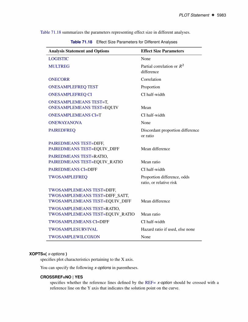
PLOT Statement F 5983
Table 71.18 summarizes the parameters representing effect size in different analyses.
Table 71.18 Effect Size Parameters for Different Analyses
Analysis Statement and Options Effect Size Parameters
LOGISTIC None
MULTREG Partial correlation or R2
difference
ONECORR Correlation
ONESAMPLEFREQ TEST Proportion
ONESAMPLEFREQ CI CI half-width
ONESAMPLEMEANS TEST=T,ONESAMPLEMEANS TEST=EQUIV Mean
ONESAMPLEMEANS CI=T CI half-width
ONEWAYANOVA None
PAIREDFREQ Discordant proportion differenceor ratio
PAIREDMEANS TEST=DIFF,PAIREDMEANS TEST=EQUIV_DIFF Mean difference
PAIREDMEANS TEST=RATIO,PAIREDMEANS TEST=EQUIV_RATIO Mean ratio
PAIREDMEANS CI=DIFF CI half-width
TWOSAMPLEFREQ Proportion difference, oddsratio, or relative risk
TWOSAMPLEMEANS TEST=DIFF,TWOSAMPLEMEANS TEST=DIFF_SATT,TWOSAMPLEMEANS TEST=EQUIV_DIFF Mean difference
TWOSAMPLEMEANS TEST=RATIO,TWOSAMPLEMEANS TEST=EQUIV_RATIO Mean ratio
TWOSAMPLEMEANS CI=DIFF CI half-width
TWOSAMPLESURVIVAL Hazard ratio if used, else none
TWOSAMPLEWILCOXON None
XOPTS=( x-options )specifies plot characteristics pertaining to the X axis.
You can specify the following x-options in parentheses.
CROSSREF=NO | YESspecifies whether the reference lines defined by the REF= x-option should be crossed with areference line on the Y axis that indicates the solution point on the curve.
5984 F Chapter 71: The POWER Procedure
REF=number-listspecifies locations for reference lines extending from the X axis across the entire plotting region.See the section “Specifying Value Lists in Analysis Statements” on page 6020 for informationabout specifying the number-list.
Y=EFFECT N POWERspecifies a plot with the requested type of parameter on the Y axis and the parameter being solvedfor on the X axis. When Y=EFFECT, the parameter assigned to the Y axis is the one most represen-tative of “effect size.” When Y=N, the parameter assigned to the Y axis is the sample size. WhenY=POWER, the parameter assigned to the Y axis is the one most representative of “power” (eitherpower itself or a similar probability, such as Prob(Width) for confidence interval analyses). You can-not use the Y= and X= options simultaneously. By default, the X= option is used instead of the Y=option.
YOPTS=( y-options )specifies plot characteristics pertaining to the Y axis.
You can specify the following y-options in parentheses.
CROSSREF=NO | YESspecifies whether the reference lines defined by the REF= y-option should be crossed with areference line on the X axis that indicates the solution point on the curve.
REF=number-listspecifies locations for reference lines extending from the Y axis across the entire plotting region.See the section “Specifying Value Lists in Analysis Statements” on page 6020 for informationabout specifying the number-list.
You can specify the following graph-options in the PLOT statement after a slash (/).
DESCRIPTION=’string ’specifies a descriptive string of up to 40 characters that appears in the “Description” field of thegraphics catalog. The description does not appear on the plots. By default, PROC POWER assigns adescription either of the form “Y versus X” (for a single-panel plot) or of the form “Y versus X (S),”where Y is the parameter on the Y axis, X is the parameter on the X axis, and S is a description of thesubset represented on the current panel of a multipanel plot.
NAME=’string ’specifies a name of up to eight characters for the catalog entry for the plot. The default name isPLOTn, where n is the number of the plot statement within the current invocation of PROC POWER.If the name duplicates the name of an existing entry, SAS/GRAPH software adds a number to theduplicate name to create a unique entry—for example, PLOT11 and PLOT12 for the second and thirdpanels of a multipanel plot generated in the first PLOT statement in an invocation of PROC POWER.
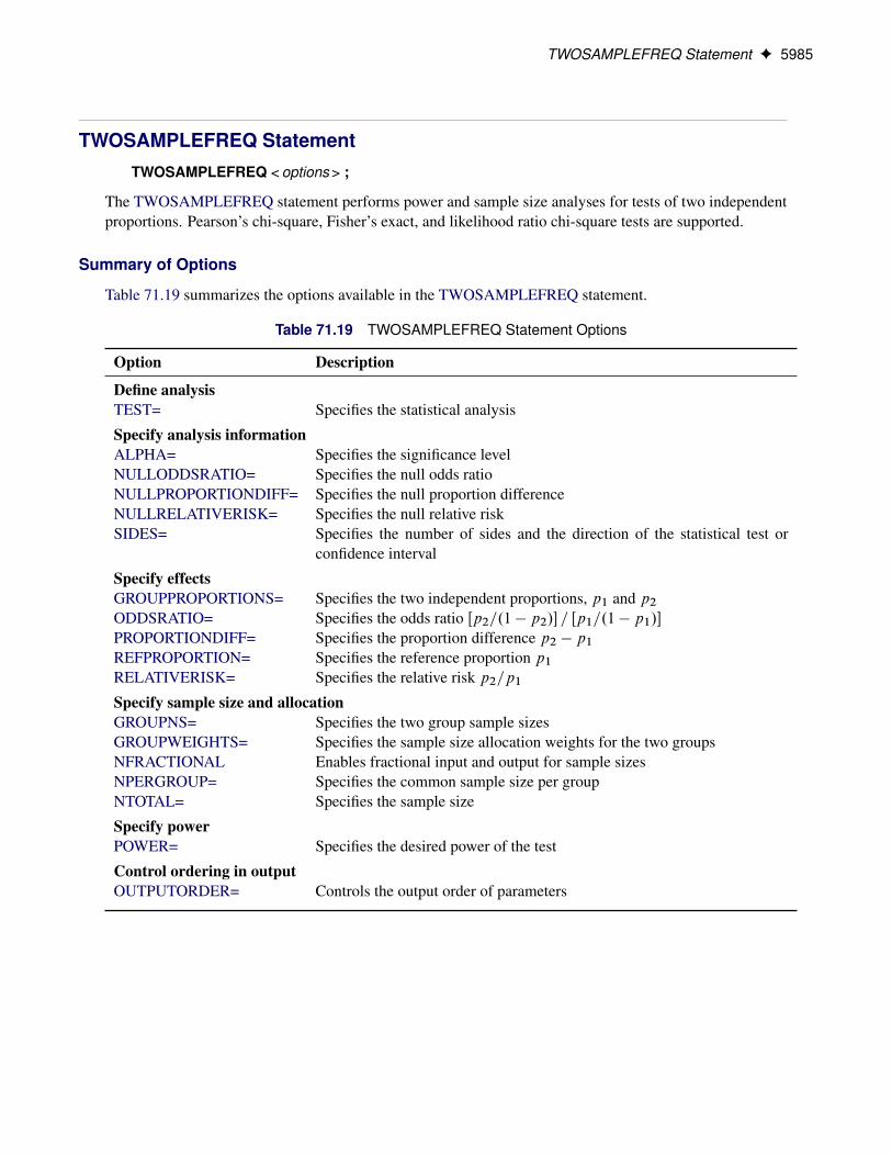
TWOSAMPLEFREQ Statement F 5985
TWOSAMPLEFREQ StatementTWOSAMPLEFREQ < options > ;
The TWOSAMPLEFREQ statement performs power and sample size analyses for tests of two independentproportions. Pearson’s chi-square, Fisher’s exact, and likelihood ratio chi-square tests are supported.
Summary of Options
Table 71.19 summarizes the options available in the TWOSAMPLEFREQ statement.
Table 71.19 TWOSAMPLEFREQ Statement Options
Option Description
Define analysisTEST= Specifies the statistical analysis
Specify analysis informationALPHA= Specifies the significance levelNULLODDSRATIO= Specifies the null odds ratioNULLPROPORTIONDIFF= Specifies the null proportion differenceNULLRELATIVERISK= Specifies the null relative riskSIDES= Specifies the number of sides and the direction of the statistical test or
confidence interval
Specify effectsGROUPPROPORTIONS= Specifies the two independent proportions, p1 and p2ODDSRATIO= Specifies the odds ratio Œp2=.1 � p2/� = Œp1=.1 � p1/�PROPORTIONDIFF= Specifies the proportion difference p2 � p1REFPROPORTION= Specifies the reference proportion p1RELATIVERISK= Specifies the relative risk p2=p1Specify sample size and allocationGROUPNS= Specifies the two group sample sizesGROUPWEIGHTS= Specifies the sample size allocation weights for the two groupsNFRACTIONAL Enables fractional input and output for sample sizesNPERGROUP= Specifies the common sample size per groupNTOTAL= Specifies the sample size
Specify powerPOWER= Specifies the desired power of the test
Control ordering in outputOUTPUTORDER= Controls the output order of parameters

5986 F Chapter 71: The POWER Procedure
Table 71.20 summarizes the valid result parameters for different analyses in the TWOSAMPLEFREQ state-ment.
Table 71.20 Summary of Result Parameters in the TWOSAMPLEFREQ Statement
Analyses Solve For Syntax
TEST=FISHER Power POWER=.Sample size NTOTAL=.
NPERGROUP=.TEST=LRCHI Power POWER=.
Sample size NTOTAL=.NPERGROUP=.
TEST=PCHI Power POWER=.Sample size NTOTAL=.
NPERGROUP=.
Dictionary of Options
ALPHA=number-listspecifies the level of significance of the statistical test. The default is 0.05, corresponding to theusual 0.05 � 100% = 5% level of significance. See the section “Specifying Value Lists in AnalysisStatements” on page 6020 for information about specifying the number-list.
GROUPPROPORTIONS=grouped-number-list
GPROPORTIONS=grouped-number-list
GROUPPS=grouped-number-list
GPS=grouped-number-listspecifies the two independent proportions, p1 and p2. See the section “Specifying Value Lists inAnalysis Statements” on page 6020 for information about specifying the grouped-number-list.
GROUPNS=grouped-number-list
GNS=grouped-number-listspecifies the two group sample sizes. See the section “Specifying Value Lists in Analysis Statements”on page 6020 for information about specifying the grouped-number-list.
GROUPWEIGHTS=grouped-number-list
GWEIGHTS=grouped-number-listspecifies the sample size allocation weights for the two groups. This option controls how the totalsample size is divided between the two groups. Each pair of values for the two groups representsrelative allocation weights. Additionally, if the NFRACTIONAL option is not used, the total samplesize is restricted to be equal to a multiple of the sum of the two group weights (so that the result-ing design has an integer sample size for each group while adhering exactly to the group allocationweights). Values must be integers unless the NFRACTIONAL option is used. The default value is (11), a balanced design with a weight of 1 for each group. See the section “Specifying Value Lists inAnalysis Statements” on page 6020 for information about specifying the grouped-number-list.

TWOSAMPLEFREQ Statement F 5987
NFRACTIONAL
NFRACenables fractional input and output for sample sizes. See the section “Sample Size Adjustment Op-tions” on page 6023 for information about the ramifications of the presence (and absence) of theNFRACTIONAL option.
NPERGROUP=number-list
NPERG=number-listspecifies the common sample size per group or requests a solution for the common sample size pergroup with a missing value (NPERGROUP=.). Use of this option implicitly specifies a balanceddesign. See the section “Specifying Value Lists in Analysis Statements” on page 6020 for informationabout specifying the number-list.
NTOTAL=number-listspecifies the sample size or requests a solution for the sample size with a missing value (NTOTAL=.).See the section “Specifying Value Lists in Analysis Statements” on page 6020 for information aboutspecifying the number-list.
NULLODDSRATIO=number-list
NULLOR=number-listspecifies the null odds ratio. The default value is 1. This option can be used only with the ODD-SRATIO= option in the TEST=PCHI analysis. See the section “Specifying Value Lists in AnalysisStatements” on page 6020 for information about specifying the number-list.
NULLPROPORTIONDIFF=number-list
NULLPDIFF=number-listspecifies the null proportion difference. The default value is 0. This option can be used only with theGROUPPROPORTIONS= or PROPORTIONDIFF= option in the TEST=PCHI analysis. See the sec-tion “Specifying Value Lists in Analysis Statements” on page 6020 for information about specifyingthe number-list.
NULLRELATIVERISK=number-list
NULLRR=number-listspecifies the null relative risk. The default value is 1. This option can be used only with the RELA-TIVERISK= option in the TEST=PCHI analysis. See the section “Specifying Value Lists in AnalysisStatements” on page 6020 for information about specifying the number-list.
ODDSRATIO=number-list
OR=number-listspecifies the odds ratio Œp2=.1 � p2/� = Œp1=.1 � p1/�. See the section “Specifying Value Lists inAnalysis Statements” on page 6020 for information about specifying the number-list.
OUTPUTORDER=INTERNAL
OUTPUTORDER=REVERSE
OUTPUTORDER=SYNTAXcontrols how the input and default analysis parameters are ordered in the output. OUT-PUTORDER=INTERNAL (the default) arranges the parameters in the output according to thefollowing order of their corresponding options:

5988 F Chapter 71: The POWER Procedure
� SIDES=� NULLPROPORTIONDIFF=� NULLODDSRATIO=� NULLRELATIVERISK=� ALPHA=� GROUPPROPORTIONS=� REFPROPORTION=� PROPORTIONDIFF=� ODDSRATIO=� RELATIVERISK=� GROUPWEIGHTS=� NTOTAL=� NPERGROUP=� GROUPNS=� POWER=
The OUTPUTORDER=SYNTAX option arranges the parameters in the output in the same order inwhich their corresponding options are specified in the TWOSAMPLEFREQ statement. The OUT-PUTORDER=REVERSE option arranges the parameters in the output in the reverse of the order inwhich their corresponding options are specified in the TWOSAMPLEFREQ statement.
POWER=number-listspecifies the desired power of the test or requests a solution for the power with a missing value(POWER=.). The power is expressed as a probability, a number between 0 and 1, rather than asa percentage. See the section “Specifying Value Lists in Analysis Statements” on page 6020 forinformation about specifying the number-list.
PROPORTIONDIFF=number-list
PDIFF=number-listspecifies the proportion difference p2 � p1. See the section “Specifying Value Lists in AnalysisStatements” on page 6020 for information about specifying the number-list.
REFPROPORTION=number-list
REFP=number-listspecifies the reference proportion p1. See the section “Specifying Value Lists in Analysis Statements”on page 6020 for information about specifying the number-list.
RELATIVERISK=number-list
RR=number-listspecifies the relative risk p2=p1. See the section “Specifying Value Lists in Analysis Statements” onpage 6020 for information about specifying the number-list.
SIDES=keyword-listspecifies the number of sides (or tails) and the direction of the statistical test or confidence interval.See the section “Specifying Value Lists in Analysis Statements” on page 6020 for information aboutspecifying the keyword-list. Valid keywords and their interpretation are as follows:
1 one-sided with alternative hypothesis in same direction as effect
2 two-sided

TWOSAMPLEFREQ Statement F 5989
U upper one-sided with alternative greater than null value
L lower one-sided with alternative less than null value
If the effect size is zero, then SIDES=1 is not permitted; instead, specify the direction of the testexplicitly in this case with either SIDES=L or SIDES=U. The default value is 2.
TEST=FISHER
TEST=LRCHI
TEST=PCHIspecifies the statistical analysis. TEST=FISHER specifies Fisher’s exact test. TEST=LRCHI specifiesthe likelihood ratio chi-square test. TEST=PCHI (the default) specifies Pearson’s chi-square test.
Restrictions on Option Combinations
To specify the proportions, choose one of the following parameterizations:
� individual proportions (by using the GROUPPROPORTIONS= option)
� difference between proportions and reference proportion (by using the PROPORTIONDIFF= andREFPROPORTION= options)
� odds ratio and reference proportion (by using the ODDSRATIO= and REFPROPORTION= options)
� relative risk and reference proportion (by using the RELATIVERISK= and REFPROPORTION= op-tions)
To specify the sample size and allocation, choose one of the following parameterizations:
� sample size per group in a balanced design (by using the NPERGROUP= option)
� total sample size and allocation weights (by using the NTOTAL= and GROUPWEIGHTS= options)
� individual group sample sizes (by using the GROUPNS= option)
Option Groups for Common Analyses
This section summarizes the syntax for the common analyses supported in the TWOSAMPLEFREQ state-ment.
Pearson Chi-Square Test for Two ProportionsYou can use the NPERGROUP= option in a balanced design and express effects in terms of the individualproportions, as in the following statements. Default values for the SIDES= and ALPHA= options specify atwo-sided test with a significance level of 0.05.
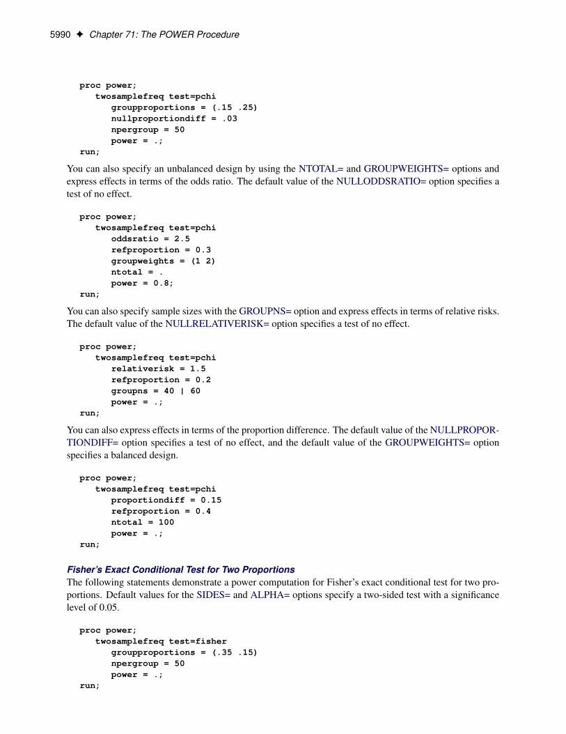
5990 F Chapter 71: The POWER Procedure
proc power;twosamplefreq test=pchi
groupproportions = (.15 .25)nullproportiondiff = .03npergroup = 50power = .;
run;
You can also specify an unbalanced design by using the NTOTAL= and GROUPWEIGHTS= options andexpress effects in terms of the odds ratio. The default value of the NULLODDSRATIO= option specifies atest of no effect.
proc power;twosamplefreq test=pchi
oddsratio = 2.5refproportion = 0.3groupweights = (1 2)ntotal = .power = 0.8;
run;
You can also specify sample sizes with the GROUPNS= option and express effects in terms of relative risks.The default value of the NULLRELATIVERISK= option specifies a test of no effect.
proc power;twosamplefreq test=pchi
relativerisk = 1.5refproportion = 0.2groupns = 40 | 60power = .;
run;
You can also express effects in terms of the proportion difference. The default value of the NULLPROPOR-TIONDIFF= option specifies a test of no effect, and the default value of the GROUPWEIGHTS= optionspecifies a balanced design.
proc power;twosamplefreq test=pchi
proportiondiff = 0.15refproportion = 0.4ntotal = 100power = .;
run;
Fisher’s Exact Conditional Test for Two ProportionsThe following statements demonstrate a power computation for Fisher’s exact conditional test for two pro-portions. Default values for the SIDES= and ALPHA= options specify a two-sided test with a significancelevel of 0.05.
proc power;twosamplefreq test=fisher
groupproportions = (.35 .15)npergroup = 50power = .;
run;

TWOSAMPLEMEANS Statement F 5991
Likelihood Ratio Chi-Square Test for Two ProportionsThe following statements demonstrate a sample size computation for the likelihood ratio chi-square testfor two proportions. Default values for the SIDES= and ALPHA= options specify a two-sided test with asignificance level of 0.05.
proc power;twosamplefreq test=lrchi
oddsratio = 2refproportion = 0.4npergroup = .power = 0.9;
run;
TWOSAMPLEMEANS StatementTWOSAMPLEMEANS < options > ;
The TWOSAMPLEMEANS statement performs power and sample size analyses for pooled and unpooled ttests, equivalence tests, and confidence interval precision involving two independent samples.
Summary of Options
Table 71.21 summarizes the options available in the TWOSAMPLEMEANS statement.
Table 71.21 TWOSAMPLEMEANS Statement Options
Option Description
Define analysisCI= Specifies an analysis of precision of the confidence intervalDIST= Specifies the underlying distribution assumed for the test statisticTEST= Specifies the statistical analysis
Specify analysis informationALPHA= Specifies the significance levelLOWER= Specifies the lower equivalence boundNULLDIFF= Specifies the null mean differenceNULLRATIO= Specifies the null mean ratioSIDES= Specifies the number of sides and the direction of the statistical test or
confidence intervalUPPER= Specifies the upper equivalence bound
Specify effectsHALFWIDTH= Specifies the desired confidence interval half-widthGROUPMEANS= Specifies the two group meansMEANDIFF= Specifies the mean differenceMEANRATIO= Specifies the geometric mean ratio, 2= 1Specify variabilityCV= Specifies the common coefficient of variation
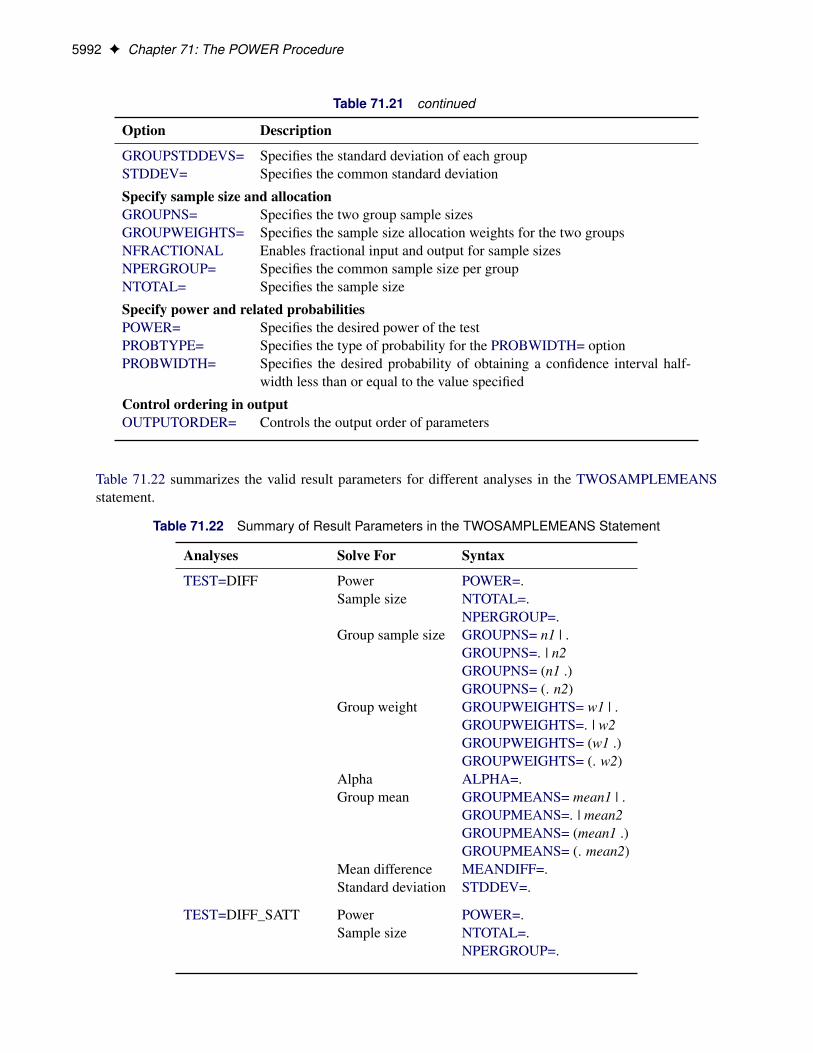
5992 F Chapter 71: The POWER Procedure
Table 71.21 continued
Option Description
GROUPSTDDEVS= Specifies the standard deviation of each groupSTDDEV= Specifies the common standard deviation
Specify sample size and allocationGROUPNS= Specifies the two group sample sizesGROUPWEIGHTS= Specifies the sample size allocation weights for the two groupsNFRACTIONAL Enables fractional input and output for sample sizesNPERGROUP= Specifies the common sample size per groupNTOTAL= Specifies the sample size
Specify power and related probabilitiesPOWER= Specifies the desired power of the testPROBTYPE= Specifies the type of probability for the PROBWIDTH= optionPROBWIDTH= Specifies the desired probability of obtaining a confidence interval half-
width less than or equal to the value specified
Control ordering in outputOUTPUTORDER= Controls the output order of parameters
Table 71.22 summarizes the valid result parameters for different analyses in the TWOSAMPLEMEANSstatement.
Table 71.22 Summary of Result Parameters in the TWOSAMPLEMEANS Statement
Analyses Solve For Syntax
TEST=DIFF Power POWER=.Sample size NTOTAL=.
NPERGROUP=.Group sample size GROUPNS= n1 | .
GROUPNS=. | n2GROUPNS= (n1 .)GROUPNS= (. n2)
Group weight GROUPWEIGHTS= w1 | .GROUPWEIGHTS=. | w2GROUPWEIGHTS= (w1 .)GROUPWEIGHTS= (. w2)
Alpha ALPHA=.Group mean GROUPMEANS= mean1 | .
GROUPMEANS=. | mean2GROUPMEANS= (mean1 .)GROUPMEANS= (. mean2)
Mean difference MEANDIFF=.Standard deviation STDDEV=.
TEST=DIFF_SATT Power POWER=.Sample size NTOTAL=.
NPERGROUP=.

TWOSAMPLEMEANS Statement F 5993
Table 71.22 continued
Analyses Solve For Syntax
TEST=RATIO Power POWER=.Sample size NTOTAL=.
NPERGROUP=.
TEST=EQUIV_DIFF Power POWER=.Sample size NTOTAL=.
NPERGROUP=.
TEST=EQUIV_RATIO Power POWER=.Sample size NTOTAL=.
NPERGROUP=.
CI=DIFF Prob(width) PROBWIDTH=.Sample size NTOTAL=.
NPERGROUP=.
Dictionary of Options
ALPHA=number-listspecifies the level of significance of the statistical test or requests a solution for alpha with a missingvalue (ALPHA=.). The default is 0.05, corresponding to the usual 0.05 � 100% = 5% level of signifi-cance. If the CI= and SIDES=1 options are used, then the value must be less than 0.5. See the section“Specifying Value Lists in Analysis Statements” on page 6020 for information about specifying thenumber-list.
CI
CI=DIFFspecifies an analysis of precision of the confidence interval for the mean difference, assuming equalvariances. Instead of power, the relevant probability for this analysis is the probability that the intervalhalf-width is at most the value specified by the HALFWIDTH= option. If neither the TEST= optionnor the CI= option is used, the default is TEST=DIFF.
CV=number-listspecifies the coefficient of variation assumed to be common to both groups. The coefficient of vari-ation is defined as the ratio of the standard deviation to the mean. You can use this option only withDIST=LOGNORMAL. See the section “Specifying Value Lists in Analysis Statements” on page 6020for information about specifying the number-list.
DIST=LOGNORMAL
DIST=NORMALspecifies the underlying distribution assumed for the test statistic. NORMAL correspondsthe normal distribution, and LOGNORMAL corresponds to the lognormal distribution. Thedefault value (also the only acceptable value in each case) is NORMAL for TEST=DIFF,TEST=DIFF_SATT, TEST=EQUIV_DIFF, and CI=DIFF; and LOGNORMAL for TEST=RATIOand TEST=EQUIV_RATIO.

5994 F Chapter 71: The POWER Procedure
GROUPMEANS=grouped-number-list
GMEANS=grouped-number-listspecifies the two group means or requests a solution for one group mean given the other. Means are inthe original scale. They are arithmetic if DIST=NORMAL and geometric if DIST=LOGNORMAL.This option cannot be used with the CI=DIFF analysis. When TEST=EQUIV_DIFF, the means areinterpreted as the reference mean (first) and the treatment mean (second). See the section “SpecifyingValue Lists in Analysis Statements” on page 6020 for information about specifying the grouped-number-list.
GROUPNS=grouped-number-list
GNS=grouped-number-listspecifies the two group sample sizes or requests a solution for one group sample size given the other.See the section “Specifying Value Lists in Analysis Statements” on page 6020 for information aboutspecifying the grouped-number-list.
GROUPSTDDEVS=grouped-number-list
GSTDDEVS=grouped-number-list
GROUPSTDS=grouped-number-list
GSTDS=grouped-number-listspecifies the standard deviation of each group. Unlike the STDDEV= option, the GROUPSTD-DEVS== option supports different values for each group. It is valid only for the Satterthwaite t test(TEST=DIFF_SATT DIST=NORMAL). See the section “Specifying Value Lists in Analysis State-ments” on page 6020 for information about specifying the grouped-number-list.
GROUPWEIGHTS=grouped-number-list
GWEIGHTS=grouped-number-listspecifies the sample size allocation weights for the two groups, or requests a solution for one groupweight given the other. This option controls how the total sample size is divided between the twogroups. Each pair of values for the two groups represents relative allocation weights. Additionally,if the NFRACTIONAL option is not used, the total sample size is restricted to be equal to a multipleof the sum of the two group weights (so that the resulting design has an integer sample size for eachgroup while adhering exactly to the group allocation weights). Values must be integers unless theNFRACTIONAL option is used. The default value is (1 1), a balanced design with a weight of 1for each group. See the section “Specifying Value Lists in Analysis Statements” on page 6020 forinformation about specifying the grouped-number-list.
HALFWIDTH=number-listspecifies the desired confidence interval half-width. The half-width is defined as the distance betweenthe point estimate and a finite endpoint. This option can be used only with the CI=DIFF analysis.See the section “Specifying Value Lists in Analysis Statements” on page 6020 for information aboutspecifying the number-list.
LOWER=number-listspecifies the lower equivalence bound for the mean difference or mean ratio, in the origi-nal scale (whether DIST=NORMAL or DIST=LOGNORMAL). Values must be greater than 0when DIST=LOGNORMAL. This option can be used only with the TEST=EQUIV_DIFF andTEST=EQUIV_RATIO analyses. See the section “Specifying Value Lists in Analysis Statements”on page 6020 for information about specifying the number-list.
TWOSAMPLEMEANS Statement F 5995
MEANDIFF=number-listspecifies the mean difference, defined as �2 � �1, or requests a solution for the mean differ-ence with a missing value (MEANDIFF=.). This option can be used only with the TEST=DIFF,TEST=DIFF_SATT, and TEST=EQUIV_DIFF analyses. When TEST=EQUIV_DIFF, the mean dif-ference is interpreted as the treatment mean minus the reference mean. See the section “SpecifyingValue Lists in Analysis Statements” on page 6020 for information about specifying the number-list.
MEANRATIO=number-listspecifies the geometric mean ratio, defined as 2= 1. This option can be used only with theTEST=RATIO and TEST=EQUIV_RATIO analyses. When TEST=EQUIV_RATIO, the mean ra-tio is interpreted as the treatment mean divided by the reference mean. See the section “SpecifyingValue Lists in Analysis Statements” on page 6020 for information about specifying the number-list.
NFRACTIONAL
NFRACenables fractional input and output for sample sizes. See the section “Sample Size Adjustment Op-tions” on page 6023 for information about the ramifications of the presence (and absence) of theNFRACTIONAL option.
NPERGROUP=number-list
NPERG=number-listspecifies the common sample size per group or requests a solution for the common sample size pergroup with a missing value (NPERGROUP=.). Use of this option implicitly specifies a balanceddesign. See the section “Specifying Value Lists in Analysis Statements” on page 6020 for informationabout specifying the number-list.
NTOTAL=number-listspecifies the sample size or requests a solution for the sample size with a missing value (NTOTAL=.).See the section “Specifying Value Lists in Analysis Statements” on page 6020 for information aboutspecifying the number-list.
NULLDIFF=number-list
NULLD=number-listspecifies the null mean difference. The default value is 0. This option can be used only with theTEST=DIFF and TEST=DIFF_SATT analyses. See the section “Specifying Value Lists in AnalysisStatements” on page 6020 for information about specifying the number-list.
NULLRATIO=number-list
NULLR=number-listspecifies the null mean ratio. The default value is 1. This option can be used only with theTEST=RATIO analysis. See the section “Specifying Value Lists in Analysis Statements” onpage 6020 for information about specifying the number-list.
OUTPUTORDER=INTERNAL
OUTPUTORDER=REVERSE
OUTPUTORDER=SYNTAXcontrols how the input and default analysis parameters are ordered in the output. OUT-PUTORDER=INTERNAL (the default) arranges the parameters in the output according to thefollowing order of their corresponding options:

5996 F Chapter 71: The POWER Procedure
� SIDES=� NULLDIFF=� NULLRATIO=� LOWER=� UPPER=� ALPHA=� GROUPMEANS=� MEANDIFF=� MEANRATIO=� HALFWIDTH=� STDDEV=� GROUPSTDDEVS==� CV=� GROUPWEIGHTS=� NTOTAL=� NPERGROUP=� GROUPNS=� POWER=� PROBTYPE=� PROBWIDTH=
The OUTPUTORDER=SYNTAX option arranges the parameters in the output in the same orderin which their corresponding options are specified in the TWOSAMPLEMEANS statement. TheOUTPUTORDER=REVERSE option arranges the parameters in the output in the reverse of the orderin which their corresponding options are specified in the TWOSAMPLEMEANS statement.
POWER=number-listspecifies the desired power of the test or requests a solution for the power with a missing value(POWER=.). The power is expressed as a probability, a number between 0 and 1, rather than asa percentage. This option cannot be used with the CI=DIFF analysis. See the section “SpecifyingValue Lists in Analysis Statements” on page 6020 for information about specifying the number-list.
PROBTYPE=keyword-listspecifies the type of probability for the PROBWIDTH= option. A value of CONDITIONAL (thedefault) indicates the conditional probability that the confidence interval half-width is at most thevalue specified by the HALFWIDTH= option, given that the true mean difference is captured bythe confidence interval. A value of UNCONDITIONAL indicates the unconditional probability thatthe confidence interval half-width is at most the value specified by the HALFWIDTH= option. youcan use the alias GIVENVALIDITY for CONDITIONAL. The PROBTYPE= option can be usedonly with the CI=DIFF analysis. See the section “Specifying Value Lists in Analysis Statements” onpage 6020 for information about specifying the keyword-list.
CONDITIONAL width probability conditional on interval containing the mean
UNCONDITIONAL unconditional width probability

TWOSAMPLEMEANS Statement F 5997
PROBWIDTH=number-listspecifies the desired probability of obtaining a confidence interval half-width less than or equal to thevalue specified by the HALFWIDTH= option. A missing value (PROBWIDTH=.) requests a solutionfor this probability. The type of probability is controlled with the PROBTYPE= option. Values areexpressed as probabilities (for example, 0.9) rather than percentages. This option can be used onlywith the CI=DIFF analysis. See the section “Specifying Value Lists in Analysis Statements” onpage 6020 for information about specifying the number-list.
SIDES=keyword-listspecifies the number of sides (or tails) and the direction of the statistical test or confidence interval.See the section “Specifying Value Lists in Analysis Statements” on page 6020 for information aboutspecifying the keyword-list. Valid keywords and their interpretation for the TEST= analyses are asfollows:
1 one-sided with alternative hypothesis in same direction as effect
2 two-sided
U upper one-sided with alternative greater than null value
L lower one-sided with alternative less than null value
For confidence intervals, SIDES=U refers to an interval between the lower confidence limit and infin-ity, and SIDES=L refers to an interval between minus infinity and the upper confidence limit. For bothof these cases and SIDES=1, the confidence interval computations are equivalent. The SIDES= op-tion cannot be used with the TEST=EQUIV_DIFF and TEST=EQUIV_RATIO analyses. The defaultvalue is 2.
STDDEV=number-list
STD=number-listspecifies the standard deviation assumed to be common to both groups, or requests a solution for thecommon standard deviation with a missing value (STDDEV=.). This option can be used only withDIST=NORMAL. See the section “Specifying Value Lists in Analysis Statements” on page 6020 forinformation about specifying the number-list.
TEST
TEST=DIFF
TEST=DIFF_SATT
TEST=EQUIV_DIFF
TEST=EQUIV_RATIO
TEST=RATIOspecifies the statistical analysis. TEST or TEST=DIFF (the default) specifies a pooled t test on themean difference, assuming equal variances. TEST=DIFF_SATT specifies a Satterthwaite unpooled ttest on the mean difference, assuming unequal variances. TEST=EQUIV_DIFF specifies an additiveequivalence test of the mean difference by using a two one-sided tests (TOST) analysis (Schuirmann1987). TEST=EQUIV_RATIO specifies a multiplicative equivalence test of the mean ratio by using aTOST analysis. TEST=RATIO specifies a pooled t test on the mean ratio, assuming equal coefficientsof variation. If neither the TEST= option nor the CI= option is used, the default is TEST=DIFF.

5998 F Chapter 71: The POWER Procedure
UPPER=number-listspecifies the upper equivalence bound for the mean difference or mean ratio, in the originalscale (whether DIST=NORMAL or DIST=LOGNORMAL). This option can be used only with theTEST=EQUIV_DIFF and TEST=EQUIV_RATIO analyses. See the section “Specifying Value Listsin Analysis Statements” on page 6020 for information about specifying the number-list.
Restrictions on Option Combinations
To define the analysis, choose one of the following parameterizations:
� a statistical test (by using the TEST= option)
� confidence interval precision (by using the CI= option)
To specify the means, choose one of the following parameterizations:
� individual group means (by using the GROUPMEANS= option)
� mean difference (by using the MEANDIFF= option)
� mean ratio (by using the MEANRATIO= option)
To specify standard deviations in the Satterthwaite t test (TEST=DIFF_SATT), choose one of the followingparameterizations:
� common standard deviation (by using the STDDEV= option)
� individual group standard deviations (by using the GROUPSTDDEVS== option)
To specify the sample sizes and allocation, choose one of the following parameterizations:
� sample size per group in a balanced design (by using the NPERGROUP= option)
� total sample size and allocation weights (by using the NTOTAL= and GROUPWEIGHTS= options)
� individual group sample sizes (by using the GROUPNS= option)
Option Groups for Common Analyses
This section summarizes the syntax for the common analyses supported in the TWOSAMPLEMEANSstatement.
Two-Sample t Test Assuming Equal VariancesYou can use the NPERGROUP= option in a balanced design and express effects in terms of the mean differ-ence, as in the following statements. Default values for the DIST=, SIDES=, NULLDIFF=, and ALPHA=options specify a two-sided test for no difference with a normal distribution and a significance level of 0.05.
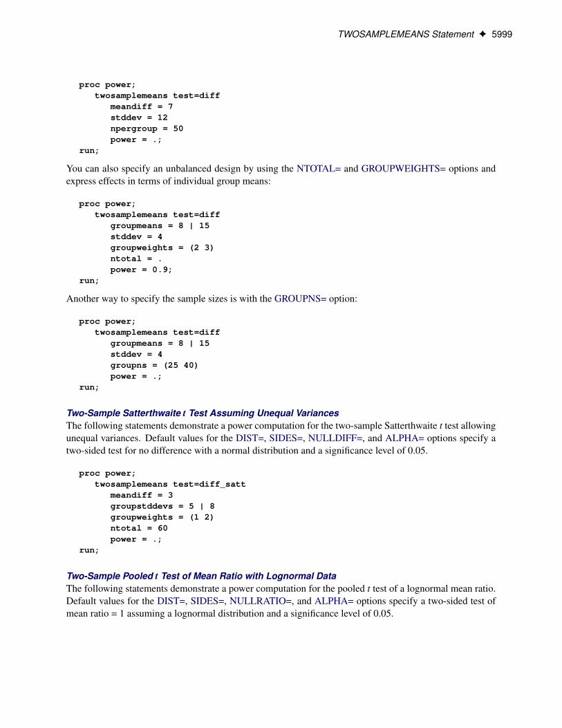
TWOSAMPLEMEANS Statement F 5999
proc power;twosamplemeans test=diff
meandiff = 7stddev = 12npergroup = 50power = .;
run;
You can also specify an unbalanced design by using the NTOTAL= and GROUPWEIGHTS= options andexpress effects in terms of individual group means:
proc power;twosamplemeans test=diff
groupmeans = 8 | 15stddev = 4groupweights = (2 3)ntotal = .power = 0.9;
run;
Another way to specify the sample sizes is with the GROUPNS= option:
proc power;twosamplemeans test=diff
groupmeans = 8 | 15stddev = 4groupns = (25 40)power = .;
run;
Two-Sample Satterthwaite t Test Assuming Unequal VariancesThe following statements demonstrate a power computation for the two-sample Satterthwaite t test allowingunequal variances. Default values for the DIST=, SIDES=, NULLDIFF=, and ALPHA= options specify atwo-sided test for no difference with a normal distribution and a significance level of 0.05.
proc power;twosamplemeans test=diff_satt
meandiff = 3groupstddevs = 5 | 8groupweights = (1 2)ntotal = 60power = .;
run;
Two-Sample Pooled t Test of Mean Ratio with Lognormal DataThe following statements demonstrate a power computation for the pooled t test of a lognormal mean ratio.Default values for the DIST=, SIDES=, NULLRATIO=, and ALPHA= options specify a two-sided test ofmean ratio = 1 assuming a lognormal distribution and a significance level of 0.05.

6000 F Chapter 71: The POWER Procedure
proc power;twosamplemeans test=ratio
meanratio = 7cv = 0.8groupns = 50 | 70power = .;
run;
Additive Equivalence Test for Mean Difference with Normal DataThe following statements demonstrate a sample size computation for the TOST equivalence test for a normalmean difference. A default value of GROUPWEIGHTS=(1 1) specifies a balanced design. Default valuesfor the DIST= and ALPHA= options specify a significance level of 0.05 and an assumption of normallydistributed data.
proc power;twosamplemeans test=equiv_diff
lower = 2upper = 5meandiff = 4stddev = 8ntotal = .power = 0.9;
run;
Multiplicative Equivalence Test for Mean Ratio with Lognormal DataThe following statements demonstrate a power computation for the TOST equivalence test for a lognormalmean ratio. Default values for the DIST= and ALPHA= options specify a significance level of 0.05 and anassumption of lognormally distributed data.
proc power;twosamplemeans test=equiv_ratio
lower = 3upper = 7meanratio = 5cv = 0.75npergroup = 50power = .;
run;
Confidence Interval for Mean DifferenceBy default CI=DIFF analyzes the conditional probability of obtaining the desired precision, given that theinterval contains the true mean difference, as in the following statements. The defaults of SIDES=2 andALPHA=0.05 specify a two-sided interval with a confidence level of 0.95.
proc power;twosamplemeans ci = diff
halfwidth = 4stddev = 8groupns = (30 35)probwidth = .;
run;

TWOSAMPLESURVIVAL Statement F 6001
TWOSAMPLESURVIVAL StatementTWOSAMPLESURVIVAL < options > ;
The TWOSAMPLESURVIVAL statement performs power and sample size analyses for comparing twosurvival curves. The log-rank, Gehan, and Tarone-Ware rank tests are supported.
Summary of Options
Table 71.23 summarizes the options available in the TWOSAMPLESURVIVAL statement.
Table 71.23 TWOSAMPLESURVIVAL Statement Options
Option Description
Define analysisTEST= Specifies the statistical analysis
Specify analysis informationACCRUALTIME= Specifies the accrual timeALPHA= Specifies the significance levelFOLLOWUPTIME= Specifies the follow-up timeSIDES= Specifies the number of sides and the direction of the statistical test or
confidence intervalTOTALTIME= Specifies the total time
Specify effectsCURVE= Defines a survival curveGROUPMEDSURVTIMES= Specifies the median survival times in each groupGROUPSURVEXPHAZARDS= Specifies exponential hazard rates of the survival curve for each groupGROUPSURVIVAL= Specifies the survival curve for each groupHAZARDRATIO= Specifies the hazard ratioREFSURVEXPHAZARD= Specifies the exponential hazard rate of the survival curve for the reference
groupREFSURVIVAL= Specifies the survival curve for the reference group
Specify loss informationGROUPLOSS= Specifies the exponential loss survival curve for each groupGROUPLOSSEXPHAZARDS= Specifies the exponential hazards of the loss in each groupGROUPMEDLOSSTIMES= Specifies the median times of the loss in each group
Specify sample size and allocationACCRUALRATEPERGROUP= Specifies the common accrual rate per groupACCRUALRATETOTAL= Specifies the total accrual rateEVENTSTOTAL= Specifies the expected total number of eventsGROUPACCRUALRATES= Specifies the accrual rate for each groupGROUPNS= Specifies the two group sample sizesGROUPWEIGHTS= Specifies the sample size allocation weights for the two groupsNFRACTIONAL Enables fractional input and output for sample sizesNPERGROUP= Specifies the common sample size per groupNTOTAL= Specifies the sample size
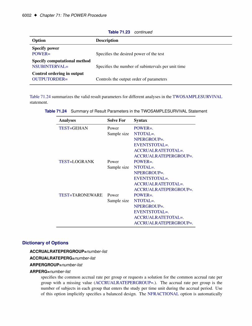
6002 F Chapter 71: The POWER Procedure
Table 71.23 continued
Option Description
Specify powerPOWER= Specifies the desired power of the test
Specify computational methodNSUBINTERVAL= Specifies the number of subintervals per unit time
Control ordering in outputOUTPUTORDER= Controls the output order of parameters
Table 71.24 summarizes the valid result parameters for different analyses in the TWOSAMPLESURVIVALstatement.
Table 71.24 Summary of Result Parameters in the TWOSAMPLESURVIVAL Statement
Analyses Solve For Syntax
TEST=GEHAN Power POWER=.Sample size NTOTAL=.
NPERGROUP=.EVENTSTOTAL=.ACCRUALRATETOTAL=.ACCRUALRATEPERGROUP=.
TEST=LOGRANK Power POWER=.Sample size NTOTAL=.
NPERGROUP=.EVENTSTOTAL=.ACCRUALRATETOTAL=.ACCRUALRATEPERGROUP=.
TEST=TARONEWARE Power POWER=.Sample size NTOTAL=.
NPERGROUP=.EVENTSTOTAL=.ACCRUALRATETOTAL=.ACCRUALRATEPERGROUP=.
Dictionary of Options
ACCRUALRATEPERGROUP=number-list
ACCRUALRATEPERG=number-list
ARPERGROUP=number-list
ARPERG=number-listspecifies the common accrual rate per group or requests a solution for the common accrual rate pergroup with a missing value (ACCRUALRATEPERGROUP=.). The accrual rate per group is thenumber of subjects in each group that enters the study per time unit during the accrual period. Useof this option implicitly specifies a balanced design. The NFRACTIONAL option is automatically

TWOSAMPLESURVIVAL Statement F 6003
enabled when the ACCRUALRATEPERGROUP= option is used. See the section “Specifying ValueLists in Analysis Statements” on page 6020 for information about specifying the number-list.
ACCRUALRATETOTAL=number-list
ARTOTAL=number-listspecifies the total accrual rate or requests a solution for the accrual rate with a missing value (AC-CRUALRATETOTAL=.). The total accrual rate is the total number of subjects that enter the studyper time unit during the accrual period. The NFRACTIONAL option is automatically enabled whenthe ACCRUALRATETOTAL= option is used. See the section “Specifying Value Lists in AnalysisStatements” on page 6020 for information about specifying the number-list.
ACCRUALTIME=number-list | MAX
ACCTIME=number-list | MAX
ACCRUALT=number-list | MAX
ACCT=number-list | MAXspecifies the accrual time. Accrual is assumed to occur uniformly from time 0 to the time specifiedby the ACCRUALTIME= option. If the GROUPSURVIVAL= or REFSURVIVAL= option is used,then the value of the total time (the sum of accrual and follow-up times) must be less than or equalto the largest time in each multipoint (piecewise linear) survival curve. If the ACCRUALRATE-PERGROUP=, ACCRUALRATETOTAL=, or GROUPACCRUALRATES= option is used, then theaccrual time must be greater than 0. See the section “Specifying Value Lists in Analysis Statements”on page 6020 for information about specifying the number-list.
ACCRUALTIME=MAX can be used when each scenario in the analysis contains at least one piece-wise linear survival curve (in the GROUPSURVIVAL= or REFSURVIVAL= option). It causes theaccrual time to be automatically set, separately for each scenario, to the maximum possible timesupported by the piecewise linear survival curve(s) in that scenario. It is not compatible with theFOLLOWUPTIME=MAX option or the TOTALTIME= option.
ALPHA=number-listspecifies the level of significance of the statistical test. The default is 0.05, corresponding to theusual 0.05 � 100% = 5% level of significance. See the section “Specifying Value Lists in AnalysisStatements” on page 6020 for information about specifying the number-list.
CURVE("label")=pointsdefines a survival curve.
For the CURVE= option,
label identifies the curve in the output and with the GROUPLOSS=, GROUPSUR-VIVAL=, and REFSURVIVAL= options.
points specifies one or more (time, survival) pairs on the curve, where the survival valuedenotes the probability of surviving until at least the specified time.

6004 F Chapter 71: The POWER Procedure
A single-point curve is interpreted as exponential, and a multipoint curve is interpreted as piecewiselinear. Points can be expressed in either of two forms:
� a series of time:survival pairs separated by spaces. For example:
1:0.9 2:0.7 3:0.6
� a DOLIST of times enclosed in parentheses, followed by a colon (:), followed by a DOLIST ofsurvival values enclosed in parentheses. For example:
(1 to 3 by 1):(0.9 0.7 0.6)
The DOLIST format is the same as in the DATA step.
Points can also be expressed as combinations of the two forms. For example:
1:0.9 2:0.8 (3 to 6 by 1):(0.7 0.65 0.6 0.55)
The points have the following restrictions:
� The time values must be nonnegative and strictly increasing.
� The survival values must be strictly decreasing.
� The survival value at a time of 0 must be equal to 1.
� If there is only one point, then the time must be greater than 0, and the survival value cannot be0 or 1.
EVENTSTOTAL=number-list
EVENTTOTAL=number-list
EETOTAL=number-listspecifies the expected total number of events—that is, deaths, whether observed or censored—duringthe entire study period, or requests a solution for this parameter with a missing value (EVENTSTO-TAL=.). The NFRACTIONAL option is automatically enabled when the EVENTSTOTAL= option isused. See the section “Specifying Value Lists in Analysis Statements” on page 6020 for informationabout specifying the number-list.
FOLLOWUPTIME=number-list | MAX
FUTIME=number-list | MAX
FOLLOWUPT=number-list | MAX
FUT=number-list | MAXspecifies the follow-up time, the amount of time in the study past the accrual time. If the GROUP-SURVIVAL= or REFSURVIVAL= option is used, then the value of the total time (the sum of accrualand follow-up times) must be less than or equal to the largest time in each multipoint (piecewise lin-ear) survival curve. See the section “Specifying Value Lists in Analysis Statements” on page 6020 forinformation about specifying the number-list.
FOLLOWUPTIME=MAX can be used when each scenario in the analysis contains at least one piece-wise linear survival curve (in the GROUPSURVIVAL= or REFSURVIVAL= option). It causes thefollow-up time to be automatically set, separately for each scenario, to the maximum possible timesupported by the piecewise linear survival curve(s) in that scenario. It is not compatible with theACCRUALTIME=MAX option or the TOTALTIME= option.

TWOSAMPLESURVIVAL Statement F 6005
GROUPACCRUALRATES=grouped-number-list
GACCRUALRATES=grouped-number-list
GROUPARS=grouped-number-list
GARS=grouped-number-listspecifies the accrual rate for each group. The groupwise accrual rates are the numbers of subjectsin each group that enters the study per time unit during the accrual period. The NFRACTIONALoption is automatically enabled when the GROUPACCRUALRATES= option is used. See the section“Specifying Value Lists in Analysis Statements” on page 6020 for information about specifying thegrouped-number-list.
GROUPLOSS=grouped-name-list
GLOSS=grouped-name-listspecifies the exponential loss survival curve for each group, by using labels specified with theCURVE= option. Loss is assumed to follow an exponential curve, indicating the expected rate ofcensoring (in other words, loss to follow-up) over time. See the section “Specifying Value Lists inAnalysis Statements” on page 6020 for information about specifying the grouped-name-list.
GROUPLOSSEXPHAZARDS=grouped-number-list
GLOSSEXPHAZARDS=grouped-number-list
GROUPLOSSEXPHS=grouped-number-list
GLOSSEXPHS=grouped-number-listspecifies the exponential hazards of the loss in each group. Loss is assumed to follow an exponen-tial curve, indicating the expected rate of censoring (in other words, loss to follow-up) over time. Ifnone of the GROUPLOSSEXPHAZARDS=, GROUPLOSS=, and GROUPMEDLOSSTIMES= op-tions are used, the default of GROUPLOSSEXPHAZARDS=(0 0) indicates no loss to follow-up.See the section “Specifying Value Lists in Analysis Statements” on page 6020 for information aboutspecifying the grouped-number-list.
GROUPMEDLOSSTIMES=grouped-number-list
GMEDLOSSTIMES=grouped-number-list
GROUPMEDLOSSTS=grouped-number-list
GMEDLOSSTS=grouped-number-listspecifies the median times of the loss in each group. Loss is assumed to follow an exponential curve,indicating the expected rate of censoring (in other words, loss to follow-up) over time. See the section“Specifying Value Lists in Analysis Statements” on page 6020 for information about specifying thegrouped-number-list.
GROUPMEDSURVTIMES=grouped-number-list
GMEDSURVTIMES=grouped-number-list
GROUPMEDSURVTS=grouped-number-list
GMEDSURVTS=grouped-number-listspecifies the median survival times in each group. When the GROUPMEDSURVTIMES= option isused, the survival curve in each group is assumed to be exponential. See the section “Specifying ValueLists in Analysis Statements” on page 6020 for information about specifying the grouped-number-list.

6006 F Chapter 71: The POWER Procedure
GROUPNS=grouped-number-list
GNS=grouped-number-listspecifies the two group sample sizes. See the section “Specifying Value Lists in Analysis Statements”on page 6020 for information about specifying the grouped-number-list.
GROUPSURVEXPHAZARDS=grouped-number-list
GSURVEXPHAZARDS=grouped-number-list
GROUPSURVEXPHS=grouped-number-list
GEXPHS=grouped-number-listspecifies exponential hazard rates of the survival curve for each group. See the section “SpecifyingValue Lists in Analysis Statements” on page 6020 for information about specifying the grouped-number-list.
GROUPSURVIVAL=grouped-name-list
GSURVIVAL=grouped-name-list
GROUPSURV=grouped-name-list
GSURV=grouped-name-listspecifies the survival curve for each group, by using labels specified with the CURVE= option. Seethe section “Specifying Value Lists in Analysis Statements” on page 6020 for information aboutspecifying the grouped-name-list.
GROUPWEIGHTS=grouped-number-list
GWEIGHTS=grouped-number-listspecifies the sample size allocation weights for the two groups. This option controls how the totalsample size is divided between the two groups. Each pair of values for the two groups representsrelative allocation weights. Additionally, if the NFRACTIONAL option is not used, the total samplesize is restricted to be equal to a multiple of the sum of the two group weights (so that the result-ing design has an integer sample size for each group while adhering exactly to the group allocationweights). Values must be integers unless the NFRACTIONAL option is used. The default value is (11), a balanced design with a weight of 1 for each group. See the section “Specifying Value Lists inAnalysis Statements” on page 6020 for information about specifying the grouped-number-list.
HAZARDRATIO=number-list
HR=number-listspecifies the hazard ratio of the second group’s survival curve to the first group’s survival curve.See the section “Specifying Value Lists in Analysis Statements” on page 6020 for information aboutspecifying the number-list.
NFRACTIONAL
NFRACenables fractional input and output for sample sizes. This option is automatically enabled whenany of the following options are used: ACCRUALRATEPERGROUP=, ACCRUALRATETOTAL=,EVENTSTOTAL=, and GROUPACCRUALRATES=. See the section “Sample Size Adjustment Op-tions” on page 6023 for information about the ramifications of the presence (and absence) of theNFRACTIONAL option.

TWOSAMPLESURVIVAL Statement F 6007
NPERGROUP=number-list
NPERG=number-listspecifies the common sample size per group or requests a solution for the common sample size pergroup with a missing value (NPERGROUP=.). Use of this option implicitly specifies a balanceddesign. See the section “Specifying Value Lists in Analysis Statements” on page 6020 for informationabout specifying the number-list.
NSUBINTERVAL=number-list
NSUBINTERVALS=number-list
NSUB=number-list
NSUBS=number-listspecifies the number of subintervals per unit time to use in internal calculations. Higher values in-crease computational time and memory requirements but generally lead to more accurate results. Thedefault value is 12. See the section “Specifying Value Lists in Analysis Statements” on page 6020 forinformation about specifying the number-list.
NTOTAL=number-listspecifies the sample size or requests a solution for the sample size with a missing value (NTOTAL=.).See the section “Specifying Value Lists in Analysis Statements” on page 6020 for information aboutspecifying the number-list.
OUTPUTORDER=INTERNAL
OUTPUTORDER=REVERSE
OUTPUTORDER=SYNTAXcontrols how the input and default analysis parameters are ordered in the output. OUT-PUTORDER=INTERNAL (the default) arranges the parameters in the output according to thefollowing order of their corresponding options:
� SIDES=� ACCRUALTIME=� FOLLOWUPTIME=� TOTALTIME=� NSUBINTERVAL=� ALPHA=� REFSURVIVAL=� GROUPSURVIVAL=� REFSURVEXPHAZARD=� HAZARDRATIO=� GROUPSURVEXPHAZARDS=� GROUPMEDSURVTIMES=� GROUPLOSSEXPHAZARDS=� GROUPLOSS=� GROUPMEDLOSSTIMES=� GROUPWEIGHTS=� NTOTAL=� ACCRUALRATETOTAL=� EVENTSTOTAL=� NPERGROUP=

6008 F Chapter 71: The POWER Procedure
� ACCRUALRATEPERGROUP=� GROUPNS=� GROUPACCRUALRATES=� POWER=
The OUTPUTORDER=SYNTAX option arranges the parameters in the output in the same order inwhich their corresponding options are specified in the TWOSAMPLESURVIVAL statement. TheOUTPUTORDER=REVERSE option arranges the parameters in the output in the reverse of the orderin which their corresponding options are specified in the TWOSAMPLESURVIVAL statement.
POWER=number-listspecifies the desired power of the test or requests a solution for the power with a missing value(POWER=.). The power is expressed as a probability, a number between 0 and 1, rather than asa percentage. See the section “Specifying Value Lists in Analysis Statements” on page 6020 forinformation about specifying the number-list.
REFSURVEXPHAZARD=number-list
REFSURVEXPH=number-listspecifies the exponential hazard rate of the survival curve for the first (reference) group. See the sec-tion “Specifying Value Lists in Analysis Statements” on page 6020 for information about specifyingthe number-list.
REFSURVIVAL=name-list
REFSURV=name-listspecifies the survival curve for the first (reference) group, by using labels specified with the CURVE=option. See the section “Specifying Value Lists in Analysis Statements” on page 6020 for informationabout specifying the name-list.
SIDES=keyword-listspecifies the number of sides (or tails) and the direction of the statistical test or confidence interval.See the section “Specifying Value Lists in Analysis Statements” on page 6020 for information aboutspecifying the keyword-list. Valid keywords and their interpretation are as follows:
1 one-sided with alternative hypothesis in same direction as effect
2 two-sided
U upper one-sided with the alternative hypothesis favoring better survival in the second group
L lower one-sided with the alternative hypothesis favoring better survival in the first (reference)group
The default value is 2.
TEST=GEHAN
TEST=LOGRANK
TEST=TARONEWAREspecifies the statistical analysis. TEST=GEHAN specifies the Gehan rank test. TEST=LOGRANK(the default) specifies the log-rank test. TEST=TARONEWARE specifies the Tarone-Ware rank test.

TWOSAMPLESURVIVAL Statement F 6009
TOTALTIME=number-list | MAX
TOTALT=number-list | MAXspecifies the total time, which is equal to the sum of accrual and follow-up times. If the GROUPSUR-VIVAL= or REFSURVIVAL= option is used, then the value of the total time must be less than or equalto the largest time in each multipoint (piecewise linear) survival curve. See the section “SpecifyingValue Lists in Analysis Statements” on page 6020 for information about specifying the number-list.
TOTALTIME=MAX can be used when each scenario in the analysis contains at least one piecewiselinear survival curve (in the GROUPSURVIVAL= or REFSURVIVAL= option). It causes the totaltime to be automatically set, separately for each scenario, to the maximum possible time supportedby the piecewise linear survival curve(s) in that scenario. It is not compatible with the ACCRUAL-TIME=MAX option or the FOLLOWUPTIME=MAX option.
Restrictions on Option Combinations
To specify the survival curves, choose one of the following parameterizations:
� arbitrary piecewise linear or exponential curves (by using the CURVE= and GROUPSURVIVAL=options)
� curves with proportional hazards (by using the CURVE=, REFSURVIVAL=, and HAZARDRATIO=options)
� exponential curves, by using one of the following parameterizations:
– median survival times (by using the GROUPMEDSURVTIMES= option)
– the hazard ratio and the hazard of the reference curve (by using the HAZARDRATIO= andREFSURVEXPHAZARD= options)
– the individual hazards (by using the GROUPSURVEXPHAZARDS= option)
To specify the study time, use any two of the following three options:
� accrual time (by using the ACCRUALTIME= option)
� follow-up time (by using the FOLLOWUPTIME= option)
� total time, the sum of accrual and follow-up times (by using the TOTALTIME= option)
To specify the sample size and allocation, choose one of the following parameterizations:
� sample size per group in a balanced design (by using the NPERGROUP= option)
� accrual rate per group in a balanced design (by using the ACCRUALRATEPERGROUP= option)
� total sample size and allocation weights (by using the NTOTAL= and GROUPWEIGHTS= options)
� total accrual rate and allocation weights (by using the ACCRUALRATETOTAL= and GROUP-WEIGHTS= options)
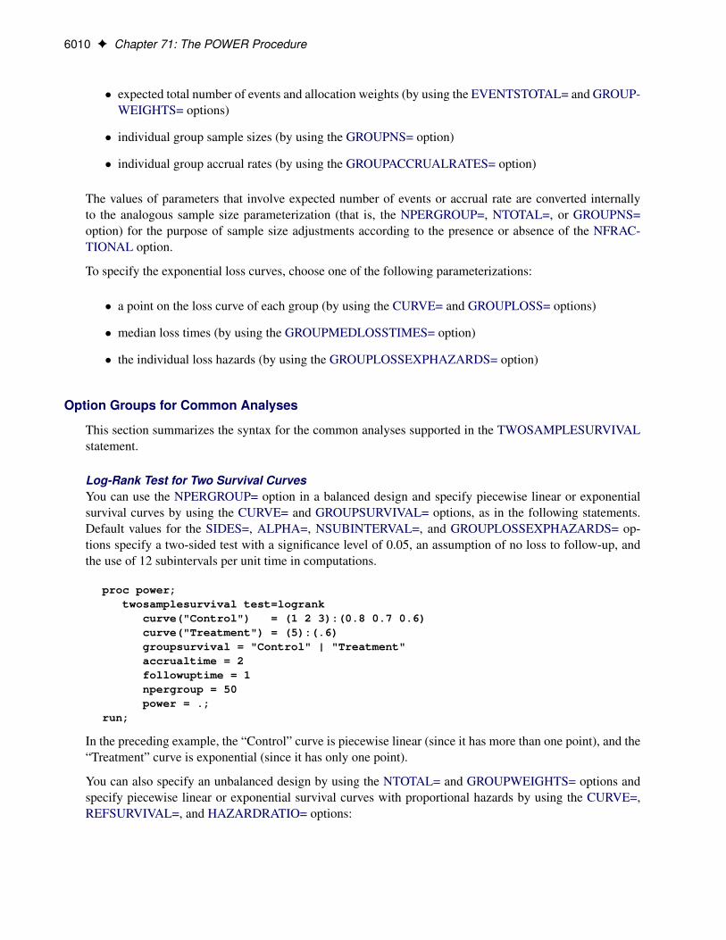
6010 F Chapter 71: The POWER Procedure
� expected total number of events and allocation weights (by using the EVENTSTOTAL= and GROUP-WEIGHTS= options)
� individual group sample sizes (by using the GROUPNS= option)
� individual group accrual rates (by using the GROUPACCRUALRATES= option)
The values of parameters that involve expected number of events or accrual rate are converted internallyto the analogous sample size parameterization (that is, the NPERGROUP=, NTOTAL=, or GROUPNS=option) for the purpose of sample size adjustments according to the presence or absence of the NFRAC-TIONAL option.
To specify the exponential loss curves, choose one of the following parameterizations:
� a point on the loss curve of each group (by using the CURVE= and GROUPLOSS= options)
� median loss times (by using the GROUPMEDLOSSTIMES= option)
� the individual loss hazards (by using the GROUPLOSSEXPHAZARDS= option)
Option Groups for Common Analyses
This section summarizes the syntax for the common analyses supported in the TWOSAMPLESURVIVALstatement.
Log-Rank Test for Two Survival CurvesYou can use the NPERGROUP= option in a balanced design and specify piecewise linear or exponentialsurvival curves by using the CURVE= and GROUPSURVIVAL= options, as in the following statements.Default values for the SIDES=, ALPHA=, NSUBINTERVAL=, and GROUPLOSSEXPHAZARDS= op-tions specify a two-sided test with a significance level of 0.05, an assumption of no loss to follow-up, andthe use of 12 subintervals per unit time in computations.
proc power;twosamplesurvival test=logrank
curve("Control") = (1 2 3):(0.8 0.7 0.6)curve("Treatment") = (5):(.6)groupsurvival = "Control" | "Treatment"accrualtime = 2followuptime = 1npergroup = 50power = .;
run;
In the preceding example, the “Control” curve is piecewise linear (since it has more than one point), and the“Treatment” curve is exponential (since it has only one point).
You can also specify an unbalanced design by using the NTOTAL= and GROUPWEIGHTS= options andspecify piecewise linear or exponential survival curves with proportional hazards by using the CURVE=,REFSURVIVAL=, and HAZARDRATIO= options:
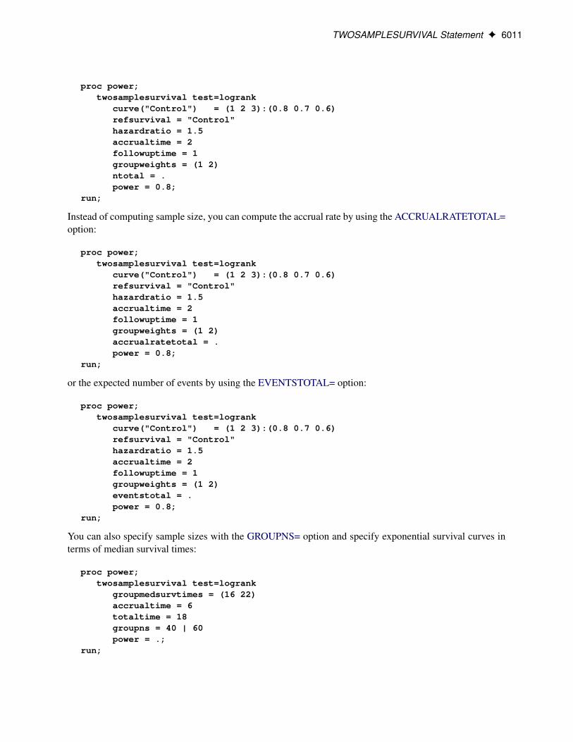
TWOSAMPLESURVIVAL Statement F 6011
proc power;twosamplesurvival test=logrank
curve("Control") = (1 2 3):(0.8 0.7 0.6)refsurvival = "Control"hazardratio = 1.5accrualtime = 2followuptime = 1groupweights = (1 2)ntotal = .power = 0.8;
run;
Instead of computing sample size, you can compute the accrual rate by using the ACCRUALRATETOTAL=option:
proc power;twosamplesurvival test=logrank
curve("Control") = (1 2 3):(0.8 0.7 0.6)refsurvival = "Control"hazardratio = 1.5accrualtime = 2followuptime = 1groupweights = (1 2)accrualratetotal = .power = 0.8;
run;
or the expected number of events by using the EVENTSTOTAL= option:
proc power;twosamplesurvival test=logrank
curve("Control") = (1 2 3):(0.8 0.7 0.6)refsurvival = "Control"hazardratio = 1.5accrualtime = 2followuptime = 1groupweights = (1 2)eventstotal = .power = 0.8;
run;
You can also specify sample sizes with the GROUPNS= option and specify exponential survival curves interms of median survival times:
proc power;twosamplesurvival test=logrank
groupmedsurvtimes = (16 22)accrualtime = 6totaltime = 18groupns = 40 | 60power = .;
run;

6012 F Chapter 71: The POWER Procedure
You can also specify exponential survival curves in terms of the hazard ratio and reference hazard. Thedefault value of the GROUPWEIGHTS= option specifies a balanced design.
proc power;twosamplesurvival test=logrank
hazardratio = 1.2refsurvexphazard = 0.7accrualtime = 2totaltime = 4ntotal = 100power = .;
run;
You can also specify exponential survival curves in terms of the individual hazards, as in the followingstatements:
proc power;twosamplesurvival test=logrank
groupsurvexphazards = 0.7 | 0.84accrualtime = 2totaltime = 4ntotal = .power = 0.9;
run;
Gehan Rank Test for Two Survival CurvesIn addition to the log-rank test, you can also specify the Gehan tank test, as in the following statements. De-fault values for the SIDES=, ALPHA=, NSUBINTERVAL=, and GROUPLOSSEXPHAZARDS= optionsspecify a two-sided test with a significance level of 0.05, an assumption of no loss to follow-up, and the useof 12 subintervals per unit time in computations.
proc power;twosamplesurvival test=gehan
groupmedsurvtimes = 5 | 7accrualtime = 3totaltime = 6npergroup = .power = 0.8;
run;
Tarone-Ware Rank Test for Two Survival CurvesYou can also specify the Tarone-Ware tank test, as in the following statements. Default values for theSIDES=, ALPHA=, NSUBINTERVAL=, and GROUPLOSSEXPHAZARDS= options specify a two-sidedtest with a significance level of 0.05, an assumption of no loss to follow-up, and the use of 12 subintervalsper unit time in computations.

TWOSAMPLEWILCOXON Statement F 6013
proc power;twosamplesurvival test=taroneware
groupmedsurvtimes = 5 | 7accrualtime = 3totaltime = 6npergroup = 100power = .;
run;
TWOSAMPLEWILCOXON StatementTWOSAMPLEWILCOXON < options > ;
The TWOSAMPLEWILCOXON statement performs power and sample size analyses for the Wilcoxon-Mann-Whitney test (also called the Wilcoxon rank-sum test, Mann-Whitney-Wilcoxon test, or Mann-Whitney U test) for two independent groups.
Note that the O’Brien-Castelloe approach to computing power for the Wilcoxon test is approximate, basedon asymptotic behavior as the total sample size gets large. The quality of the power approximation de-grades for small sample sizes; conversely, the quality of the sample size approximation degrades if the twodistributions are far apart, so that only a small sample is needed to detect a significant difference. Butthis degradation is rarely a problem in practical situations, in which experiments are usually performed forrelatively close distributions.
Summary of Options
Table 71.25 summarizes the options available in the TWOSAMPLEWILCOXON statement.
Table 71.25 TWOSAMPLEWILCOXON Statement Options
Option Description
Define analysisTEST= Specifies the statistical analysis
Specify analysis informationALPHA= Specifies the significance levelSIDES= Specifies the number of sides and the direction of the statistical test
Specify distributionsVARDIST= Defines a distribution for a variableVARIABLES= Specifies the distributions of two or more variables
Specify sample size and allocationGROUPNS= Specifies the two group sample sizesGROUPWEIGHTS= Specifies the sample size allocation weights for the two groupsNFRACTIONAL Enables fractional input and output for sample sizesNPERGROUP= Specifies the common sample size per groupNTOTAL= Specifies the sample size
Specify powerPOWER= Specifies the desired power of the test

6014 F Chapter 71: The POWER Procedure
Table 71.25 continued
Option Description
Specify computational optionsNBINS= Specifies the number of categories for each variable
Control ordering in outputOUTPUTORDER= Controls the output order of parameters
Table 71.26 summarizes the valid result parameters in the TWOSAMPLEWILCOXON statement.
Table 71.26 Summary of Result Parameters in the TWOSAMPLEWILCOXON Statement
Analyses Solve For Syntax
TEST=WMW Power POWER=.Sample size NTOTAL=.
NPERGROUP=.
Dictionary of Options
ALPHA=number-listspecifies the level of significance of the statistical test. The default is 0.05, corresponding to theusual 0.05 � 100% = 5% level of significance. See the section “Specifying Value Lists in AnalysisStatements” on page 6020 for information about specifying the number-list.
GROUPNS=grouped-number-list
GNS=grouped-number-listspecifies the two group sample sizes. See the section “Specifying Value Lists in Analysis Statements”on page 6020 for information about specifying the grouped-number-list.
GROUPWEIGHTS=grouped-number-list
GWEIGHTS=grouped-number-listspecifies the sample size allocation weights for the two groups. This option controls how the totalsample size is divided between the two groups. Each pair of values for the two groups representsrelative allocation weights. Additionally, if the NFRACTIONAL option is not used, the total samplesize is restricted to be equal to a multiple of the sum of the two group weights (so that the result-ing design has an integer sample size for each group while adhering exactly to the group allocationweights). Values must be integers unless the NFRACTIONAL option is used. The default value is (11), a balanced design with a weight of 1 for each group. See the section “Specifying Value Lists inAnalysis Statements” on page 6020 for information about specifying the grouped-number-list.
NBINS=number-listspecifies the number of categories (or “bins”) each variable’s distribution is divided into (unless it isordinal, in which case the categories remain intact) in internal calculations. Higher values increasecomputational time and memory requirements but generally lead to more accurate results. However,if the value is too high, then numerical instability can occur. The default value is 1000. See the section“Specifying Value Lists in Analysis Statements” on page 6020 for information about specifying thenumber-list.

TWOSAMPLEWILCOXON Statement F 6015
NFRACTIONAL
NFRACenables fractional input and output for sample sizes. See the section “Sample Size Adjustment Op-tions” on page 6023 for information about the ramifications of the presence (and absence) of theNFRACTIONAL option.
NPERGROUP=number-list
NPERG=number-listspecifies the common sample size per group or requests a solution for the common sample size pergroup with a missing value (NPERGROUP=.). Use of this option implicitly specifies a balanceddesign. See the section “Specifying Value Lists in Analysis Statements” on page 6020 for informationabout specifying the number-list.
NTOTAL=number-listspecifies the sample size or requests a solution for the sample size with a missing value (NTOTAL=.).See the section “Specifying Value Lists in Analysis Statements” on page 6020 for information aboutspecifying the number-list.
OUTPUTORDER=INTERNAL
OUTPUTORDER=REVERSE
OUTPUTORDER=SYNTAXcontrols how the input and default analysis parameters are ordered in the output. OUT-PUTORDER=INTERNAL (the default) arranges the parameters in the output according to thefollowing order of their corresponding options:
� SIDES� NBINS=� ALPHA=� VARIABLES=� GROUPWEIGHTS=� NTOTAL=� NPERGROUP=� GROUPNS=� POWER=
The OUTPUTORDER=SYNTAX option arranges the parameters in the output in the same order inwhich their corresponding options are specified in the TWOSAMPLEWILCOXON statement. TheOUTPUTORDER=REVERSE option arranges the parameters in the output in the reverse of the orderin which their corresponding options are specified in the TWOSAMPLEWILCOXON statement.
POWER=number-listspecifies the desired power of the test or requests a solution for the power with a missing value(POWER=.). The power is expressed as a probability, a number between 0 and 1, rather than asa percentage. See the section “Specifying Value Lists in Analysis Statements” on page 6020 forinformation about specifying the number-list.

6016 F Chapter 71: The POWER Procedure
SIDES=keyword-listspecifies the number of sides (or tails) and the direction of the statistical test. Valid keywords are asfollows:
1 one-sided with alternative hypothesis in same direction as effect
2 two-sided
U upper one-sided with alternative greater than null value
L lower one-sided with alternative less than null value
The default value is 2.
TEST=WMWspecifies the Wilcoxon-Mann-Whitney test for two independent groups This is the default test option.
VARDIST("label")=distribution (parameters)defines a distribution for a variable.
For the VARDIST= option,
label identifies the variable distribution in the output and with the VARIABLES= option.
distribution specifies the distributional form of the variable.
parameters specifies one or more parameters associated with the distribution.
Choices for distributional forms and their parameters are as follows:
ORDINAL ((values) : (probabilities)) is an ordered categorical distribution. The values are anynumbers separated by spaces. The probabilities are numbers between 0 and 1 (inclusive) sep-arated by spaces. Their sum must be exactly 1. The number of probabilities must match thenumber of values.
BETA (a, b <, l, r >) is a beta distribution with shape parameters a and b and optional location pa-rameters l and r. The values of a and b must be greater than 0, and l must be less than r. Thedefault values for l and r are 0 and 1, respectively.
BINOMIAL (p, n) is a binomial distribution with probability of success p and number of indepen-dent Bernoulli trials n. The value of p must be greater than 0 and less than 1, and n must be aninteger greater than 0. If n = 1, then the distribution is binary.
EXPONENTIAL (�) is an exponential distribution with scale �, which must be greater than 0.
GAMMA (a, �) is a gamma distribution with shape a and scale �. The values of a and � must begreater than 0.
LAPLACE (� , �) is a Laplace distribution with location � and scale �. The value of � must begreater than 0.
LOGISTIC (� , �) is a logistic distribution with location � and scale �. The value of � must begreater than 0.
LOGNORMAL (� , �) is a lognormal distribution with location � and scale �. The value of � mustbe greater than 0.
NORMAL (� , �) is a normal distribution with mean � and standard deviation �. The value of �must be greater than 0.
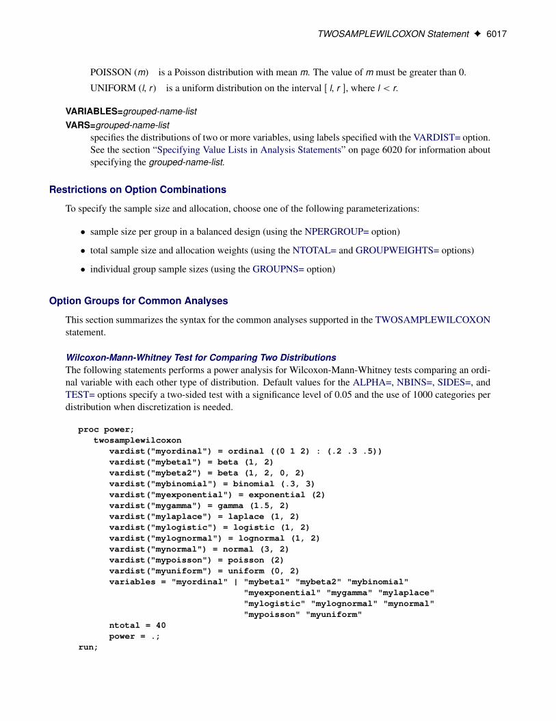
TWOSAMPLEWILCOXON Statement F 6017
POISSON (m) is a Poisson distribution with mean m. The value of m must be greater than 0.
UNIFORM (l, r ) is a uniform distribution on the interval Œ l, r �, where l < r.
VARIABLES=grouped-name-listVARS=grouped-name-list
specifies the distributions of two or more variables, using labels specified with the VARDIST= option.See the section “Specifying Value Lists in Analysis Statements” on page 6020 for information aboutspecifying the grouped-name-list.
Restrictions on Option Combinations
To specify the sample size and allocation, choose one of the following parameterizations:
� sample size per group in a balanced design (using the NPERGROUP= option)
� total sample size and allocation weights (using the NTOTAL= and GROUPWEIGHTS= options)
� individual group sample sizes (using the GROUPNS= option)
Option Groups for Common Analyses
This section summarizes the syntax for the common analyses supported in the TWOSAMPLEWILCOXONstatement.
Wilcoxon-Mann-Whitney Test for Comparing Two DistributionsThe following statements performs a power analysis for Wilcoxon-Mann-Whitney tests comparing an ordi-nal variable with each other type of distribution. Default values for the ALPHA=, NBINS=, SIDES=, andTEST= options specify a two-sided test with a significance level of 0.05 and the use of 1000 categories perdistribution when discretization is needed.
proc power;twosamplewilcoxon
vardist("myordinal") = ordinal ((0 1 2) : (.2 .3 .5))vardist("mybeta1") = beta (1, 2)vardist("mybeta2") = beta (1, 2, 0, 2)vardist("mybinomial") = binomial (.3, 3)vardist("myexponential") = exponential (2)vardist("mygamma") = gamma (1.5, 2)vardist("mylaplace") = laplace (1, 2)vardist("mylogistic") = logistic (1, 2)vardist("mylognormal") = lognormal (1, 2)vardist("mynormal") = normal (3, 2)vardist("mypoisson") = poisson (2)vardist("myuniform") = uniform (0, 2)variables = "myordinal" | "mybeta1" "mybeta2" "mybinomial"
"myexponential" "mygamma" "mylaplace""mylogistic" "mylognormal" "mynormal""mypoisson" "myuniform"
ntotal = 40power = .;
run;

6018 F Chapter 71: The POWER Procedure
Details: POWER Procedure
Overview of Power ConceptsIn statistical hypothesis testing, you typically express the belief that some effect exists in a population byspecifying an alternative hypothesis H1. You state a null hypothesis H0 as the assertion that the effect doesnot exist and attempt to gather evidence to reject H0 in favor of H1. Evidence is gathered in the form ofsample data, and a statistical test is used to assess H0. If H0 is rejected but there really is no effect, thisis called a Type I error. The probability of a Type I error is usually designated “alpha” or ˛, and statisticaltests are designed to ensure that ˛ is suitably small (for example, less than 0.05).
If there really is an effect in the population but H0 is not rejected in the statistical test, then a Type II errorhas been made. The probability of a Type II error is usually designated “beta” or ˇ. The probability 1�ˇ ofavoiding a Type II error—that is, correctly rejecting H0 and achieving statistical significance—is called thepower. (NOTE: Another more general definition of power is the probability of rejecting H0 for any givenset of circumstances, even those corresponding to H0 being true. The POWER procedure uses this moregeneral definition.)
An important goal in study planning is to ensure an acceptably high level of power. Sample size plays aprominent role in power computations because the focus is often on determining a sufficient sample size toachieve a certain power, or assessing the power for a range of different sample sizes.
Some of the analyses in the POWER procedure focus on precision rather than power. An analysis of confi-dence interval precision is analogous to a traditional power analysis, with “CI Half-Width” taking the placeof effect size and “Prob(Width)” taking the place of power. The CI Half-Width is the margin of error associ-ated with the confidence interval, the distance between the point estimate and an endpoint. The Prob(Width)is the probability of obtaining a confidence interval with at most a target half-width.
Summary of AnalysesTable 71.27 gives a summary of the analyses supported in the POWER procedure. The name of the analysisstatement reflects the type of data and design. The TEST=, CI=, and DIST= options specify the focus ofthe statistical hypothesis (in other words, the criterion on which the research question is based) and the teststatistic to be used in data analysis.
Table 71.27 Summary of Analyses
Analysis Statement Options
Logistic regression: likelihood ratiochi-square test
LOGISTIC
Multiple linear regression: Type III F test MULTREG
Correlation: Fisher’s z test ONECORR DIST=FISHERZ
Correlation: t test ONECORR DIST=T
Binomial proportion: exact test ONESAMPLEFREQ TEST=EXACT
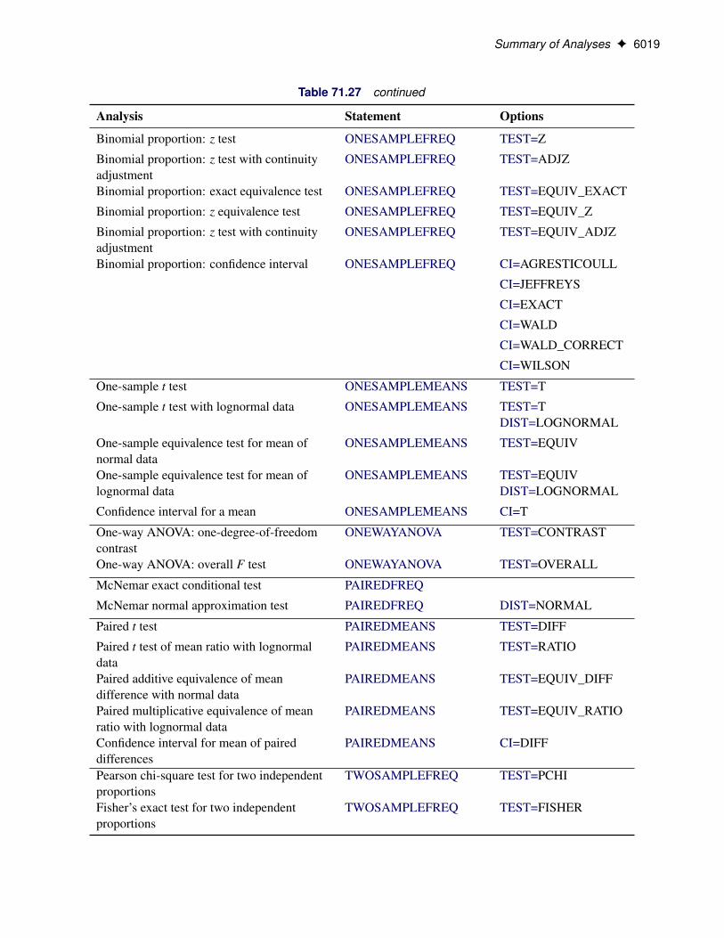
Summary of Analyses F 6019
Table 71.27 continued
Analysis Statement Options
Binomial proportion: z test ONESAMPLEFREQ TEST=Z
Binomial proportion: z test with continuityadjustment
ONESAMPLEFREQ TEST=ADJZ
Binomial proportion: exact equivalence test ONESAMPLEFREQ TEST=EQUIV_EXACT
Binomial proportion: z equivalence test ONESAMPLEFREQ TEST=EQUIV_Z
Binomial proportion: z test with continuityadjustment
ONESAMPLEFREQ TEST=EQUIV_ADJZ
Binomial proportion: confidence interval ONESAMPLEFREQ CI=AGRESTICOULL
CI=JEFFREYS
CI=EXACT
CI=WALD
CI=WALD_CORRECT
CI=WILSON
One-sample t test ONESAMPLEMEANS TEST=T
One-sample t test with lognormal data ONESAMPLEMEANS TEST=TDIST=LOGNORMAL
One-sample equivalence test for mean ofnormal data
ONESAMPLEMEANS TEST=EQUIV
One-sample equivalence test for mean oflognormal data
ONESAMPLEMEANS TEST=EQUIVDIST=LOGNORMAL
Confidence interval for a mean ONESAMPLEMEANS CI=T
One-way ANOVA: one-degree-of-freedomcontrast
ONEWAYANOVA TEST=CONTRAST
One-way ANOVA: overall F test ONEWAYANOVA TEST=OVERALL
McNemar exact conditional test PAIREDFREQ
McNemar normal approximation test PAIREDFREQ DIST=NORMAL
Paired t test PAIREDMEANS TEST=DIFF
Paired t test of mean ratio with lognormaldata
PAIREDMEANS TEST=RATIO
Paired additive equivalence of meandifference with normal data
PAIREDMEANS TEST=EQUIV_DIFF
Paired multiplicative equivalence of meanratio with lognormal data
PAIREDMEANS TEST=EQUIV_RATIO
Confidence interval for mean of paireddifferences
PAIREDMEANS CI=DIFF
Pearson chi-square test for two independentproportions
TWOSAMPLEFREQ TEST=PCHI
Fisher’s exact test for two independentproportions
TWOSAMPLEFREQ TEST=FISHER

6020 F Chapter 71: The POWER Procedure
Table 71.27 continued
Analysis Statement Options
Likelihood ratio chi-square test for twoindependent proportions
TWOSAMPLEFREQ TEST=LRCHI
Two-sample t test assuming equal variances TWOSAMPLEMEANS TEST=DIFF
Two-sample Satterthwaite t test assumingunequal variances
TWOSAMPLEMEANS TEST=DIFF_SATT
Two-sample pooled t test of mean ratio withlognormal data
TWOSAMPLEMEANS TEST=RATIO
Two-sample additive equivalence of meandifference with normal data
TWOSAMPLEMEANS TEST=EQUIV_DIFF
Two-sample multiplicative equivalence ofmean ratio with lognormal data
TWOSAMPLEMEANS TEST=EQUIV_RATIO
Two-sample confidence interval for meandifference
TWOSAMPLEMEANS CI=DIFF
Log-rank test for comparing two survivalcurves
TWOSAMPLESURVIVAL TEST=LOGRANK
Gehan rank test for comparing two survivalcurves
TWOSAMPLESURVIVAL TEST=GEHAN
Tarone-Ware rank test for comparing twosurvival curves
TWOSAMPLESURVIVAL TEST=TARONEWARE
Wilcoxon-Mann-Whitney (rank-sum) test TWOSAMPLEWILCOXON
Specifying Value Lists in Analysis StatementsTo specify one or more scenarios for an analysis parameter (or set of parameters), you provide a list ofvalues for the statement option that corresponds to the parameter(s). To identify the parameter you want tosolve for, you place missing values in the appropriate list.
There are five basic types of such lists: keyword-lists, number-lists, grouped-number-lists, name-lists, andgrouped-name-lists. Some parameters, such as the direction of a test, have values represented by one ormore keywords in a keyword-list. Scenarios for scalar-valued parameters, such as power, are representedby a number-list. Scenarios for groups of scalar-valued parameters, such as group sample sizes in a multi-group design, are represented by a grouped-number-list. Scenarios for named parameters, such as referencesurvival curves, are represented by a name-list. Scenarios for groups of named parameters, such as groupsurvival curves, are represented by a grouped-name-list.
The following subsections explain these five basic types of lists.
Keyword-Lists
A keyword-list is a list of one or more keywords separated by spaces. For example, you can specify bothtwo-sided and upper-tailed versions of a one-sample t test:
SIDES = 2 U

Specifying Value Lists in Analysis Statements F 6021
Number-Lists
A number-list can be one of two things: a series of one or more numbers expressed in the form of one ormore DOLISTs, or a missing value indicator (.).
The DOLIST format is the same as in the DATA step language. For example, for the one-sample t test youcan specify four scenarios (30, 50, 70, and 100) for a total sample size in any of the following ways.
NTOTAL = 30 50 70 100NTOTAL = 30 to 70 by 20 100
A missing value identifies a parameter as the result parameter; it is valid only with options representingparameters you can solve for in a given analysis. For example, you can request a solution for NTOTAL:
NTOTAL = .
Grouped-Number-Lists
A grouped-number-list specifies multiple scenarios for numeric values in two or more groups, possiblyincluding missing value indicators to solve for a specific group. The list can assume one of two generalforms, a “crossed” version and a “matched” version.
Crossed Grouped-Number-ListsThe crossed version of a grouped number list consists of a series of number-lists (see the section “Number-Lists” on page 6021), one representing each group, with groups separated by a vertical bar (|). The valuesfor each group represent multiple scenarios for that group, and the scenarios for each individual group arecrossed to produce the set of all scenarios for the analysis option. For example, you can specify the followingsix scenarios for the sizes .n1; n2/ of two groups
.20; 30/.20; 40/.20; 50/
.25; 30/.25; 40/.25; 50/
as follows:
GROUPNS = 20 25 | 30 40 50
If the analysis can solve for a value in one group given the other groups, then one of the number-lists in acrossed grouped-number-list can be a missing value indicator (.). For example, in a two-sample t test youcan posit three scenarios for the group 2 sample size while solving for the group 1 sample size:
GROUPNS = . | 30 40 50
Some analyses can involve more than two groups. For example, you can specify 2 � 3 � 1 = 6 scenarios forthe means of three groups in a one-way ANOVA as follows:
GROUPMEANS = 10 12 | 10 to 20 by 5 | 24

6022 F Chapter 71: The POWER Procedure
Matched Grouped-Number-ListsThe matched version of a grouped number list consists of a series of numeric lists, each enclosed in paren-theses. Each list consists of a value for each group and represents a single scenario for the analysis option.Multiple scenarios for the analysis option are represented by multiple lists. For example, you can expressthe crossed grouped-number-list
GROUPNS = 20 25 | 30 40 50
alternatively in a matched format:
GROUPNS = (20 30) (20 40) (20 50) (25 30) (25 40) (25 50)
The matched version is particularly useful when you want to include only a subset of all combinations ofindividual group values. For example, you might want to pair 20 only with 50, and 25 only with 30 and 40:
GROUPNS = (20 50) (25 30) (25 40)
If the analysis can solve for a value in one group given the other groups, then you can replace the value forthat group with a missing value indicator (.). If used, the missing value indicator must occur in the samegroup in every scenario. For example, you can solve for the group 1 sample size (as in the section “CrossedGrouped-Number-Lists” on page 6021) by using a matched format:
GROUPNS = (. 30) (. 40) (. 50)
Some analyses can involve more than two groups. For example, you can specify two scenarios for the meansof three groups in a one-way ANOVA:
GROUPMEANS = (15 24 32) (12 25 36)
Name-Lists
A name-list is a list of one or more names in single or double quotes, separated by spaces. For example,you can specify two scenarios for the reference survival curve in a log-rank test:
REFSURVIVAL = "Curve A" "Curve B"
Grouped-Name-Lists
A grouped-name-list specifies multiple scenarios for names in two or more groups. The list can assume oneof two general forms, a “crossed” version and a “matched” version.

Sample Size Adjustment Options F 6023
Crossed Grouped-Name-ListsThe crossed version of a grouped name list consists of a series of name-lists (see the section “Name-Lists”on page 6022), one representing each group, with groups separated by a vertical bar (|). The values for eachgroup represent multiple scenarios for that group, and the scenarios for each individual group are crossedto produce the set of all scenarios for the analysis option. For example, you can specify the following sixscenarios for the survival curves .c1; c2/ of two groups
.“Curve A”; “Curve C”/.“Curve A”; “Curve D”/.“Curve A”; “Curve E”/
.“Curve B”; “Curve C”/.“Curve B”; “Curve D”/.“Curve B”; “Curve E”/
as follows:
GROUPSURVIVAL = "Curve A" "Curve B" | "Curve C" "Curve D""Curve E"
Matched Grouped-Name-ListsThe matched version of a grouped name list consists of a series of name lists, each enclosed in parentheses.Each list consists of a name for each group and represents a single scenario for the analysis option. Multiplescenarios for the analysis option are represented by multiple lists. For example, you can express the crossedgrouped-name-list
GROUPSURVIVAL = "Curve A" "Curve B" | "Curve C" "Curve D""Curve E"
alternatively in a matched format:
GROUPSURVIVAL = ("Curve A" "Curve C")("Curve A" "Curve D")("Curve A" "Curve E")("Curve B" "Curve C")("Curve B" "Curve D")("Curve B" "Curve E")
The matched version is particularly useful when you want to include only a subset of all combinations ofindividual group values. For example, you might want to pair “Curve A” only with “Curve C”, and “CurveB” only with “Curve D” and “Curve E”:
GROUPSURVIVAL = ("Curve A" "Curve C")("Curve B" "Curve D")("Curve B" "Curve E")
Sample Size Adjustment OptionsBy default, PROC POWER rounds sample sizes conservatively (down in the input, up in the output) so thatall total sizes (and individual group sample sizes, if a multigroup design) are integers. This is generallyconsidered conservative because it selects the closest realistic design providing at most the power of the

6024 F Chapter 71: The POWER Procedure
(possibly fractional) input or mathematically optimized design. In addition, in a multigroup design, all groupsizes are adjusted to be multiples of the corresponding group weights. For example, if GROUPWEIGHTS= (2 6), then all group 1 sample sizes become multiples of 2, and all group 2 sample sizes become multiplesof 6 (and all total sample sizes become multiples of 8).
With the NFRACTIONAL option, sample size input is not rounded, and sample size output (whether totalor groupwise) are reported in two versions, a raw “fractional” version and a “ceiling” version rounded up tothe nearest integer.
Whenever an input sample size is adjusted, both the original (“nominal”) and adjusted (“actual”) samplesizes are reported. Whenever computed output sample sizes are adjusted, both the original input (“nominal”)power and the achieved (“actual”) power at the adjusted sample size are reported.
Error and Information OutputThe Error column in the main output table provides reasons for missing results and flags numerical resultsthat are bounds rather than exact answers. For example, consider the sample size analysis implemented bythe following statements:
proc power;twosamplefreq test=pchi
method=normaloddsratio= 1.0001refproportion=.4nulloddsratio=1power=.9ntotal=.;
run;
Figure 71.6 Error Column
The POWER ProcedurePearson Chi-square Test for Two Proportions
Fixed Scenario Elements
Distribution Asymptotic normalMethod Normal approximationNull Odds Ratio 1Reference (Group 1) Proportion 0.4Odds Ratio 1.0001Nominal Power 0.9Number of Sides 2Alpha 0.05Group 1 Weight 1Group 2 Weight 1

Error and Information Output F 6025
Figure 71.6 continued
Computed N Total
ActualPower N Total Error
0.206 2.15E+09 Solution is a lower bound
The output in Figure 71.6 reveals that the sample size to achieve a power of 0.9 could not be computed, butthat the sample size 2.15E+09 achieves a power of 0.206.
The Info column provides further details about Error column entries, warnings about any boundary condi-tions detected, and notes about any adjustments to input. Note that the Info column is hidden by default inthe main output. You can view it by using the ODS OUTPUT statement to save the output as a data set andthe PRINT procedure. For example, the following SAS statements print both the Error and Info columnsfor a power computation in a two-sample t test:
proc power;twosamplemeans
meandiff= 0 7stddev=2ntotal=2 5power=.;
ods output output=Power;run;
proc print noobs data=Power;var MeanDiff NominalNTotal NTotal Power Error Info;
run;
The output is shown in Figure 71.7.
Figure 71.7 Error and Info Columns
Mean NominalDiff NTotal NTotal Power Error Info
0 2 2 . Invalid input N too small / No effect0 5 4 0.050 Input N adjusted / No effect7 2 2 . Invalid input N too small7 5 4 0.477 Input N adjusted
The mean difference of 0 specified with the MEANDIFF= option leads to a “No effect” message to appearin the Info column. The sample size of 2 specified with the NTOTAL= option leads to an “Invalid input”message in the Error column and an “NTotal too small” message in the Info column. The sample size of5 leads to an “Input N adjusted” message in the Info column because it is rounded down to 4 to produceinteger group sizes of 2 per group.

6026 F Chapter 71: The POWER Procedure
Displayed OutputIf you use the PLOTONLY option in the PROC POWER statement, the procedure displays only graphicaloutput. Otherwise, the displayed output of the POWER procedure includes the following:
� the “Fixed Scenario Elements” table, which shows all applicable single-valued analysis parameters, inthe following order: distribution, method, parameters input explicitly, and parameters supplied withdefaults
� an output table showing the following when applicable (in order): the index of the scenario, all mul-tivalued input, ancillary results, the primary computed result, and error descriptions
� plots (if requested)
For each input parameter, the order of the input values is preserved in the output.
Ancillary results include the following:
� Actual Power, the achieved power, if it differs from the input (Nominal) power value
� Actual Prob(Width), the achieved precision probability, if it differs from the input (Nominal) proba-bility value
� Actual Alpha, the achieved significance level, if it differs from the input (Nominal) alpha value
� fractional sample size, if the NFRACTIONAL option is used in the analysis statement
If sample size is the result parameter and the NFRACTIONAL option is used in the analysis statement, thenboth “Fractional” and “Ceiling” sample size results are displayed. Fractional sample sizes correspond to the“Nominal” values of power or precision probability. Ceiling sample sizes are simply the fractional samplesizes rounded up to the nearest integer; they correspond to “Actual” values of power or precision probability.
ODS Table NamesPROC POWER assigns a name to each table that it creates. You can use these names to reference the tablewhen using the Output Delivery System (ODS) to select tables and create output data sets. These namesare listed in Table 71.28. For more information about ODS, see Chapter 20, “Using the Output DeliverySystem.”

Computational Resources F 6027
Table 71.28 ODS Tables Produced by PROC POWER
ODS Table Name Description Statement
FixedElements Factoid with single-valued analysis parameters Default*Output All input and computed analysis parameters, error messages, and
information messages for each scenarioDefault
PlotContent Data contained in plots, including analysis parameters and indicesidentifying plot features. (NOTE: This table is saved as a data setand not displayed in PROC POWER output.)
PLOT
*Depends on input.
Computational Resources
Memory
In the TWOSAMPLESURVIVAL statement, the amount of required memory is roughly proportional to theproduct of the number of subintervals (specified by the NSUBINTERVAL= option) and the total time of thestudy (specified by the ACCRUALTIME=, FOLLOWUPTIME=, and TOTALTIME= options). If you runout of memory, then you can try either specifying a smaller number of subintervals, changing the time scaleto a use a longer time unit (for example, years instead of months), or both.
CPU Time
In the Satterthwaite t test analysis (TWOSAMPLEMEANS TEST=DIFF_SATT), the required CPU timegrows as the mean difference decreases relative to the standard deviations. In the PAIREDFREQ statement,the required CPU time for the exact power computation (METHOD=EXACT) grows with the sample size.
Computational Methods and FormulasThis section describes the approaches used in PROC POWER to compute power for each analysis. The firstsubsection defines some common notation. The following subsections describe the various power analyses,including discussions of the data, statistical test, and power formula for each analysis. Unless otherwiseindicated, computed values for parameters besides power (for example, sample size) are obtained by solvingpower formulas for the desired parameters.
Common Notation
Table 71.29 displays notation for some of the more common parameters across analyses. The AssociatedSyntax column shows examples of relevant analysis statement options, where applicable.

6028 F Chapter 71: The POWER Procedure
Table 71.29 Common Notation
Symbol Description Associated Syntax
˛ Significance level ALPHA=N Total sample size NTOTAL=, NPAIRS=ni Sample size in ith group NPERGROUP=,
GROUPNS=wi Allocation weight for ith group (standardized to sum
to 1)GROUPWEIGHTS=
� (Arithmetic) mean MEAN=�i (Arithmetic) mean in ith group GROUPMEANS=,
PAIREDMEANS=�diff (Arithmetic) mean difference, �2 � �1 or �T � �R MEANDIFF=�0 Null mean or mean difference (arithmetic) NULL=, NULLDIFF= Geometric mean MEAN= i Geometric mean in ith group GROUPMEANS=,
PAIREDMEANS= 0 Null mean or mean ratio (geometric) NULL=, NULLRATIO=� Standard deviation (or common standard deviation
per group)STDDEV=
�i Standard deviation in ith group GROUPSTDDEVS=,PAIREDSTDDEVS=
�diff Standard deviation of differencesCV Coefficient of variation, defined as the ratio of the
standard deviation to the (arithmetic) meanCV=, PAIREDCVS=
� Correlation CORR=�T ; �R Treatment and reference (arithmetic) means for
equivalence testGROUPMEANS=,PAIREDMEANS=
T ; R Treatment and reference geometric means forequivalence test
GROUPMEANS=,PAIREDMEANS=
�L Lower equivalence bound LOWER=�U Upper equivalence bound UPPER=t .�; ı/ t distribution with df � and noncentrality ıF.�1; �2; �/ F distribution with numerator df �1, denominator df
�2, and noncentrality �tpI� pth percentile of t distribution with df �FpI�1;�2 pth percentile of F distribution with numerator df �1
and denominator df �2Bin.N; p/ Binomial distribution with sample size N and
proportion p
A “lower one-sided” test is associated with SIDES=L (or SIDES=1 with the effect smaller than the nullvalue), and an “upper one-sided” test is associated with SIDES=U (or SIDES=1 with the effect larger thanthe null value).

Computational Methods and Formulas F 6029
Owen (1965) defines a function, known as Owen’s Q, that is convenient for representing terms in powerformulas for confidence intervals and equivalence tests:
Q�.t; ıI a; b/ D
p2�
�.�2/2��22
Z b
a
ˆ
�txp�� ı
�x��1�.x/dx
where �.�/ andˆ.�/ are the density and cumulative distribution function of the standard normal distribution,respectively.
Analyses in the LOGISTIC Statement
Likelihood Ratio Chi-Square Test for One Predictor (TEST=LRCHI)The power computing formula is based on Shieh and O’Brien (1998); Shieh (2000); Self, Mauritsen, andOhara (1992), and Hsieh (1989).
Define the following notation for a logistic regression analysis:
N D # subjects (NTOTAL)
K D # predictors (not counting intercept)
x D .x1; : : : ; xK/0 D random variables for predictor vector
x�1 D .x2; : : : ; xK/0
� D .�1; : : : ; �K/0D Ex D mean predictor vector
xi D .xi1; : : : ; xiK/0 D predictor vector for subject i .i 2 1; : : : ; N /
Y D random variable for response (0 or 1)
Yi D response for subject i .i 2 1; : : : ; N /
pi D Prob.Yi D 1jxi / .i 2 1; : : : ; N /
� D Prob.Yi D 1jxi D �/ (RESPONSEPROB)
Uj D unit change for j th predictor (UNITS)
ORj D Odds.Yi D 1jxij D c/=Odds.Yi D 1jxij D c � Uj / .c arbitrary; i 2 1; : : : ; N;
j 2 1; : : : ; K/ (TESTODDSRATIO if j = 1, COVODDSRATIOS if j > 1)
‰0 D intercept in full model (INTERCEPT)
‰ D .‰1; : : : ; ‰K/0D regression coefficients in full model
(‰1 = TESTREGCOEFF, others = COVREGCOEFFS)
� D Corr.x�1; x1/ (CORR)
cj D # distinct possible values of xij (j 2 1; : : : ; K) (for any i) (NBINS)
x?gj D gth possible value of xij (g 2 1; : : : ; cj ) (j 2 1; : : : ; K)
(for any i) (VARDIST)
�gj D Prob�xij D x
?gj
�(g 2 1; : : : ; cj ) (j 2 1; : : : ; K)
(for any i) (VARDIST)
C D
KYjD1
cj D # possible values of xi (for any i)
x?m D mth possible value of xi .m 2 1; : : : ; C /
�m D Prob�xi D x?m
�.m 2 1; : : : ; C /

6030 F Chapter 71: The POWER Procedure
The logistic regression model is
log�
pi
1 � pi
�D ‰0 C‰
0xi
The hypothesis test of the first predictor variable is
H0W‰1 D 0
H1W‰1 ¤ 0
Assuming independence among all predictor variables, �m is defined as follows:
�m D
KYjD1
�h.m;j /j .m 2 1; : : : ; C /
where h.m; j / is calculated according to the following algorithm:
z D mI
do j D K to 1I
h.m; j / D mod.z � 1; cj /C 1Iz D floor..z � 1/=cj /C 1I
endI
This algorithm causes the elements of the transposed vector fh.m; 1/; : : : ; h.m;K/g to vary fastest to slow-est from right to left as m increases, as shown in the following table of h.m; j / values:
j
h.m; j / 1 2 � � � K � 1 K
1 1 1 � � � 1 1
1 1 1 � � � 1 2:::
:::::: 1 1 � � � 1 cK::: 1 1 � � � 2 1::: 1 1 � � � 2 2:::
:::
m::: 1 1 � � � 2 cK:::
:::::: c1 c2 � � � cK�1 1::: c1 c2 � � � cK�1 2:::
:::
C c1 c2 � � � cK�1 cK
The x?m values are determined in a completely analogous manner.
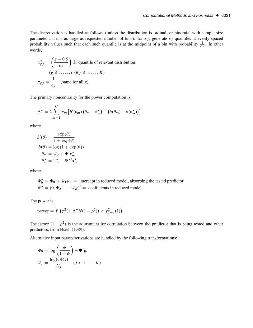
Computational Methods and Formulas F 6031
The discretization is handled as follows (unless the distribution is ordinal, or binomial with sample sizeparameter at least as large as requested number of bins): for xj , generate cj quantiles at evenly spacedprobability values such that each such quantile is at the midpoint of a bin with probability 1
cj. In other
words,
x?gj D
�g � 0:5
cj
�th quantile of relevant distribution;
.g 2 1; : : : ; cj /.j 2 1; : : : ; K/
�gj D1
cj(same for all g)
The primary noncentrality for the power computation is
�? D 2
CXmD1
�m�b0.�m/
��m � �
?m
���b.�m/ � b.�
?m/��
where
b0.�/ Dexp.�/
1C exp.�/b.�/ D log .1C exp.�//�m D ‰0 C‰
0x?m�?m D ‰
?0 C‰
?0x?m
where
‰?0 D ‰0 C‰1�1 D intercept in reduced model, absorbing the tested predictor
‰? D .0;‰2; : : : ; ‰K/0D coefficients in reduced model
The power is
power D P��2.1;�?N.1 � �2// � �21�˛.1/
�The factor .1 � �2/ is the adjustment for correlation between the predictor that is being tested and otherpredictors, from Hsieh (1989).
Alternative input parameterizations are handled by the following transformations:
‰0 D log�
�
1 � �
��‰ 0�
‰j Dlog.ORj /
Uj.j 2 1; : : : ; K/

6032 F Chapter 71: The POWER Procedure
Analyses in the MULTREG Statement
Type III F Test in Multiple Regression (TEST=TYPE3)Maxwell (2000) discusses a number of different ways to represent effect sizes (and to compute exact powerbased on them) in multiple regression. PROC POWER supports two of these, multiple partial correlationand R2 in full and reduced models.
Let p denote the total number of predictors in the full model (excluding the intercept), and let Y denote theresponse variable. You are testing that the coefficients of p1 � 1 predictors in a set X1 are 0, controlling forall of the other predictors X�1, which consists of p � p1 � 0 variables.
The hypotheses can be expressed in two different ways. The first is in terms of �YX1jX�1 , the multiplepartial correlation between the predictors in X1 and the response Y adjusting for the predictors in X�1:
H0W�2YX1jX�1
D 0
H1W�2YX1jX�1
> 0
The second is in terms of the multiple correlations in full (�Y j.X1;X�1/) and reduced (�Y jX�1) nested models:
H0W�2Y j.X1;X�1/
� �2Y jX�1 D 0
H1W�2Y j.X1;X�1/
� �2Y jX�1 > 0
Note that the squared values of �Y j.X1;X�1/ and �Y jX�1 are the population R2 values for full and reducedmodels.
The test statistic can be written in terms of the sample multiple partial correlation RYX1jX�1 ,
F D
8̂̂<̂:̂.N � 1 � p/
R2YX1jX�1
1�R2YX1jX�1
; intercept
.N � p/R2YX1jX�1
1�R2YX1jX�1
; no intercept
or the sample multiple correlations in full (RY j.X1;X�1/) and reduced (RY jX�1) models,
F D
8̂̂<̂:̂.N � 1 � p/
R2Y j.X1;X�1/
�R2Y jX�1
1�R2Y j.X1;X�1/
; intercept
.N � p/R2Y j.X1;X�1/
�R2Y jX�1
1�R2Y j.X1;X�1/
; no intercept
The test is the usual Type III F test in multiple regression:
Reject H0 if�F � F1�˛.p1; N � 1 � p/; interceptF � F1�˛.p1; N � p/; no intercept
Although the test is invariant to whether the predictors are assumed to be random or fixed, the power isaffected by this assumption. If the response and predictors are assumed to have a joint multivariate normal

Computational Methods and Formulas F 6033
distribution, then the exact power is given by the following formula:
power D
8̂̂<̂:̂P
��N�1�pp1
�� R2YX1jX�1
1�R2YX1jX�1
�� F1�˛.p1; N � 1 � p/
�; intercept
P
��N�pp1
�� R2YX1jX�1
1�R2YX1jX�1
�� F1�˛.p1; N � p/
�; no intercept
D
8̂̂<̂:̂P
�R2YX1jX�1
�F1�˛.p1;N�1�p/
F1�˛.p1;N�1�p/CN�1�pp1
�; intercept
P
�R2YX1jX�1
�F1�˛.p1;N�p/
F1�˛.p1;N�p/CN�pp1
�; no intercept
The distribution ofR2YX1jX�1
(for any �2YX1jX�1
) is given in Chapter 32 of Johnson, Kotz, and Balakrishnan(1995). Sample size tables are presented in Gatsonis and Sampson (1989).
If the predictors are assumed to have fixed values, then the exact power is given by the noncentral F distri-bution. The noncentrality parameter is
� D N�2YX1jX�1
1 � �2YX1jX�1
or equivalently,
� D N�2Y j.X1;X�1/
� �2Y jX�1
1 � �2Y j.X1;X�1/
The power is
power D�P .F.p1; N � 1 � p; �/ � F1�˛.p1; N � 1 � p// ; interceptP .F.p1; N � p; �/ � F1�˛.p1; N � p// ; no intercept
The minimum acceptable input value of N depends on several factors, as shown in Table 71.30.
Table 71.30 Minimum Acceptable Sample Size Values in the MULTREG Statement
Predictor Type Intercept in Model? p1 D 1? Minimum N
Random Yes Yes p + 3Random Yes No p + 2Random No Yes p + 2Random No No p + 1Fixed Yes Yes or No p + 2Fixed No Yes or No p + 1

6034 F Chapter 71: The POWER Procedure
Analyses in the ONECORR Statement
Fisher’s z Test for Pearson Correlation (TEST=PEARSON DIST=FISHERZ)Fisher’s z transformation (Fisher 1921) of the sample correlation RY j.X1;X�1/ is defined as
z D1
2log
�1CRY j.X1;X�1/
1 �RY j.X1;X�1/
�Fisher’s z test assumes the approximate normal distribution N.�; �2/ for z, where
� D1
2log
�1C �Y j.X1;X�1/
1 � �Y j.X1;X�1/
�C
�Y j.X1;X�1/
2.N � 1 � p?/
and
�2 D1
N � 3 � p?
where p? is the number of variables partialed out (Anderson 1984, pp. 132–133) and �Y j.X1;X�1/ is thepartial correlation between Y and X1 adjusting for the set of zero or more variables X�1.
The test statistic
z? D .N � 3 � p?/12
�z �
1
2log
�1C �0
1 � �0
��
�0
2.N � 1 � p?/
�is assumed to have a normal distribution N.ı; �/, where �0 is the null partial correlation and ı and � arederived from Section 16.33 of Stuart and Ord (1994):
ı D .N � 3 � p?/12
"1
2log
�1C �Y j.X1;X�1/
1 � �Y j.X1;X�1/
�C
�Y j.X1;X�1/
2.N � 1 � p?/
1C
5C �2Y j.X1;X�1/
4.N � 1 � p?/C
11C 2�2Y j.X1;X�1/
C 3�4Y j.X1;X�1/
8.N � 1 � p?/2
!�1
2log
�1C �0
1 � �0
��
�0
2.N � 1 � p?/
#
� DN � 3 � p?
N � 1 � p?
"1C
4 � �2Y j.X1;X�1/
2.N � 1 � p?/C
22 � 6�2Y j.X1;X�1/
� 3�4Y j.X1;X�1/
6.N � 1 � p?/2
#
The approximate power is computed as
power D
8̂̂̂̂ˆ̂<̂ˆ̂̂̂̂:
ˆ
�ı�z1�˛
�12
�; upper one-sided
ˆ
��ı�z1�˛
�12
�; lower one-sided
ˆ
�ı�z1�˛
2
�12
�Cˆ
��ı�z1�˛
2
�12
�; two-sided
Because the test is biased, the achieved significance level might differ from the nominal significance level.The actual alpha is computed in the same way as the power except with the correlation �Y j.X1;X�1/ replacedby the null correlation �0.

Computational Methods and Formulas F 6035
t Test for Pearson Correlation (TEST=PEARSON DIST=T)The two-sided case is identical to multiple regression with an intercept and p1 D 1, which is discussed inthe section “Analyses in the MULTREG Statement” on page 6032.
Let p? denote the number of variables partialed out. For the one-sided cases, the test statistic is
t D .N � 2 � p?/12
RYX1jX�1�1 �R2
YX1jX�1
� 12
which is assumed to have a null distribution of t .N � 2 � p?/.
If the X and Y variables are assumed to have a joint multivariate normal distribution, then the exact poweris given by the following formula:
power D
8̂̂̂̂ˆ̂<̂ˆ̂̂̂̂:P
24.N � 2 � p?/ 12 RYX1jX�1�1�R2
YX1jX�1
� 12
� t1�˛.N � 2 � p?/
35 ; upper one-sided
P
24.N � 2 � p?/ 12 RYX1jX�1�1�R2
YX1jX�1
� 12
� t˛.N � 2 � p?/
35 ; lower one-sided
D
8̂̂̂̂<̂ˆ̂̂:P
"RY j.X1;X�1/ �
t1�˛.N�2�p?/
.t21�˛.N�2�p?/CN�2�p?/12
#; upper one-sided
P
"RY j.X1;X�1/ �
t˛.N�2�p?/
.t2˛.N�2�p?/CN�2�p?/12
#; lower one-sided
The distribution of RY j.X1;X�1/ (given the underlying true correlation �Y j.X1;X�1/) is given in Chapter 32of Johnson, Kotz, and Balakrishnan (1995).
If the X variables are assumed to have fixed values, then the exact power is given by the noncentral tdistribution t .N � 2 � p?; ı/, where the noncentrality is
ı D N12
�YX1jX�1�1 � �2
YX1jX�1
� 12
The power is
power D�P .t.N � 2 � p?; ı/ � t1�˛.N � 2 � p
?// ; upper one-sidedP .t.N � 2 � p?; ı/ � t˛.N � 2 � p
?// ; lower one-sided

6036 F Chapter 71: The POWER Procedure
Analyses in the ONESAMPLEFREQ Statement
Exact Test of a Binomial Proportion (TEST=EXACT)Let X be distributed as Bin.N; p/. The hypotheses for the test of the proportion p are as follows:
H0Wp D p0
H1W
8<:p ¤ p0; two-sidedp > p0; upper one-sidedp < p0; lower one-sided
The exact test assumes binomially distributed data and requires N � 1 and 0 < p0 < 1. The test statistic is
X D number of successes Ï Bin.N; p/
The significance probability ˛ is split symmetrically for two-sided tests, in the sense that each tail is filledwith as much as possible up to ˛=2.
Exact power computations are based on the binomial distribution and computing formulas such as the fol-lowing from Johnson, Kotz, and Kemp (1992, equation 3.20):
P.X � C jN;p/ D P
�F�1;�2 �
�2p
�1.1 � p/
�where �1 D 2C and �2 D 2.N � C C 1/
Let CL and CU denote lower and upper critical values, respectively. Let ˛a denote the achieved (actual)significance level, which for two-sided tests is the sum of the favorable major tail (˛M ) and the oppositeminor tail (˛m).
For the upper one-sided case,
CU D minfC W P.X � C jp0/ � ˛gReject H0 if X � CU
˛a D P.X � CU jp0/
power D P.X � CU jp/
For the lower one-sided case,
CL D maxfC W P.X � C jp0/ � ˛gReject H0 if X � CL
˛a D P.X � CLjp0/
power D P.X � CLjp/
For the two-sided case,
CL D maxfC W P.X � C jp0/ �˛
2g
CU D minfC W P.X � C jp0/ �˛
2g
Reject H0 if X � CL orX � CU˛a D P.X � CL orX � CU jp0/
power D P.X � CL orX � CU jp/

Computational Methods and Formulas F 6037
z Test for Binomial Proportion Using Null Variance (TEST=Z VAREST=NULL)For the normal approximation test, the test statistic is
Z.X/ DX �Np0
ŒNp0.1 � p0/�12
For the METHOD=EXACT option, the computations are the same as described in the section “Exact Testof a Binomial Proportion (TEST=EXACT)” on page 6036 except for the definitions of the critical values.
For the upper one-sided case,
CU D minfC W Z.C/ � z1�˛g
For the lower one-sided case,
CL D maxfC W Z.C/ � z˛g
For the two-sided case,
CL D maxfC W Z.C/ � z˛2g
CU D minfC W Z.C/ � z1�˛2g
For the METHOD=NORMAL option, the test statistic Z.X/ is assumed to have the normal distribution
N
N12 .p � p0/
Œp0.1 � p0/�12
;p.1 � p/
p0.1 � p0/
!
The approximate power is computed as
power D
8̂̂̂̂ˆ̂̂̂̂<̂ˆ̂̂̂̂̂̂:̂
ˆ
z˛CpN
p�p0pp0.1�p0/q
p.1�p/p0.1�p0/
!; upper one-sided
ˆ
z˛�pN
p�p0pp0.1�p0/q
p.1�p/p0.1�p0/
!; lower one-sided
ˆ
z˛2CpN
p�p0pp0.1�p0/q
p.1�p/p0.1�p0/
!Cˆ
z˛2�pN
p�p0pp0.1�p0/q
p.1�p/p0.1�p0/
!; two-sided
The approximate sample size is computed in closed form for the one-sided cases by inverting the powerequation,
N D
zpower
pp.1 � p/C z1�˛
pp0.1 � p0/
p � p0
!2and by numerical inversion for the two-sided case.

6038 F Chapter 71: The POWER Procedure
z Test for Binomial Proportion Using Sample Variance (TEST=Z VAREST=SAMPLE)For the normal approximation test using the sample variance, the test statistic is
Zs.X/ DX �Np0
ŒN Op.1 � Op/�12
where Op D X=N .
For the METHOD=EXACT option, the computations are the same as described in the section “Exact Testof a Binomial Proportion (TEST=EXACT)” on page 6036 except for the definitions of the critical values.
For the upper one-sided case,
CU D minfC W Zs.C / � z1�˛g
For the lower one-sided case,
CL D maxfC W Zs.C / � z˛g
For the two-sided case,
CL D maxfC W Zs.C / � z˛2g
CU D minfC W Zs.C / � z1�˛2g
For the METHOD=NORMAL option, the test statistic Zs.X/ is assumed to have the normal distribution
N
N
12 .p � p0/
Œp.1 � p/�12
; 1
!
(see Chow, Shao, and Wang (2003, p. 82)).
The approximate power is computed as
power D
8̂̂̂<̂ˆ̂:ˆ�z˛ C
pN p�p0p
p.1�p/
�; upper one-sided
ˆ�z˛ �
pN p�p0p
p.1�p/
�; lower one-sided
ˆ�z˛2CpN p�p0p
p.1�p/
�Cˆ
�z˛2�pN p�p0p
p.1�p/
�; two-sided
The approximate sample size is computed in closed form for the one-sided cases by inverting the powerequation,
N D p.1 � p/
�zpower C z1�˛
p � p0
�2and by numerical inversion for the two-sided case.

Computational Methods and Formulas F 6039
z Test for Binomial Proportion with Continuity Adjustment Using Null Variance (TEST=ADJZVAREST=NULL)For the normal approximation test with continuity adjustment, the test statistic is (Pagano and Gauvreau1993, p. 295):
Zc.X/ DX �Np0 C 0:5.1fX<Np0g/ � 0:5.1fX>Np0g/
ŒNp0.1 � p0/�12
For the METHOD=EXACT option, the computations are the same as described in the section “Exact Testof a Binomial Proportion (TEST=EXACT)” on page 6036 except for the definitions of the critical values.
For the upper one-sided case,
CU D minfC W Zc.C / � z1�˛g
For the lower one-sided case,
CL D maxfC W Zc.C / � z˛g
For the two-sided case,
CL D maxfC W Zc.C / � z˛2g
CU D minfC W Zc.C / � z1�˛2g
For the METHOD=NORMAL option, the test statistic Zc.X/ is assumed to have the normal distributionN.�; �2/, where � and �2 are derived as follows.
For convenience of notation, define
k D1
2pNp0.1 � p0/
Then
E ŒZc.X/� D 2kNp � 2kNp0 C kP.X < Np0/ � kP.X > Np0/
and
Var ŒZc.X/� D 4k2Np.1 � p/C k2 Œ1 � P.X D Np0/� � k2 ŒP.X < Np0/ � P.X > Np0/�2
C 4k2�E�X1fX<Np0g
��E
�X1fX>Np0g
��� 4k2Np ŒP.X < Np0/ � P.X > Np0/�
The probabilities P.X D Np0/, P.X < Np0/, and P.X > Np0/ and the truncated expectationsE�X1fX<Np0g
�and E
�X1fX>Np0g
�are approximated by assuming the normal-approximate distribution
of X,N.Np;Np.1�p//. Letting �.�/ andˆ.�/ denote the standard normal PDF and CDF, respectively, anddefining d as
d DNp0 �Np
ŒNp.1 � p/�12

6040 F Chapter 71: The POWER Procedure
the terms are computed as follows:
P.X D Np0/ D 0
P.X < Np0/ D ˆ.d/
P.X > Np0/ D 1 �ˆ.d/
E�X1fX<Np0g
�D Npˆ.d/ � ŒNp.1 � p/�
12 �.d/
E�X1fX>Np0g
�D Np Œ1 �ˆ.d/�C ŒNp.1 � p/�
12 �.d/
The mean and variance of Zc.X/ are thus approximated by
� D k Œ2Np � 2Np0 C 2ˆ.d/ � 1�
and
�2 D 4k2hNp.1 � p/Cˆ.d/ .1 �ˆ.d// � 2 .Np.1 � p//
12 �.d/
iThe approximate power is computed as
power D
8̂̂̂<̂ˆ̂:ˆ�z˛C��
�; upper one-sided
ˆ�z˛��
�
�; lower one-sided
ˆ
�z˛2C�
�
�Cˆ
�z˛2��
�
�; two-sided
The approximate sample size is computed by numerical inversion.
z Test for Binomial Proportion with Continuity Adjustment Using Sample Variance (TEST=ADJZVAREST=SAMPLE)For the normal approximation test with continuity adjustment using the sample variance, the test statistic is
Zcs.X/ DX �Np0 C 0:5.1fX<Np0g/ � 0:5.1fX>Np0g/
ŒN Op.1 � Op/�12
where Op D X=N .
For the METHOD=EXACT option, the computations are the same as described in the section “Exact Testof a Binomial Proportion (TEST=EXACT)” on page 6036 except for the definitions of the critical values.
For the upper one-sided case,
CU D minfC W Zcs.C / � z1�˛g
For the lower one-sided case,
CL D maxfC W Zcs.C / � z˛g

Computational Methods and Formulas F 6041
For the two-sided case,
CL D maxfC W Zcs.C / � z˛2g
CU D minfC W Zcs.C / � z1�˛2g
For the METHOD=NORMAL option, the test statistic Zcs.X/ is assumed to have the normal distributionN.�; �2/, where � and �2 are derived as follows.
For convenience of notation, define
k D1
2pNp.1 � p/
Then
E ŒZcs.X/� � 2kNp � 2kNp0 C kP.X < Np0/ � kP.X > Np0/
and
Var ŒZcs.X/� � 4k2Np.1 � p/C k2 Œ1 � P.X D Np0/� � k2 ŒP.X < Np0/ � P.X > Np0/�2
C 4k2�E�X1fX<Np0g
��E
�X1fX>Np0g
��� 4k2Np ŒP.X < Np0/ � P.X > Np0/�
The probabilities P.X D Np0/, P.X < Np0/, and P.X > Np0/ and the truncated expectationsE�X1fX<Np0g
�and E
�X1fX>Np0g
�are approximated by assuming the normal-approximate distribution
of X,N.Np;Np.1�p//. Letting �.�/ andˆ.�/ denote the standard normal PDF and CDF, respectively, anddefining d as
d DNp0 �Np
ŒNp.1 � p/�12
the terms are computed as follows:
P.X D Np0/ D 0
P.X < Np0/ D ˆ.d/
P.X > Np0/ D 1 �ˆ.d/
E�X1fX<Np0g
�D Npˆ.d/ � ŒNp.1 � p/�
12 �.d/
E�X1fX>Np0g
�D Np Œ1 �ˆ.d/�C ŒNp.1 � p/�
12 �.d/
The mean and variance of Zcs.X/ are thus approximated by
� D k Œ2Np � 2Np0 C 2ˆ.d/ � 1�
and
�2 D 4k2hNp.1 � p/Cˆ.d/ .1 �ˆ.d// � 2 .Np.1 � p//
12 �.d/
i

6042 F Chapter 71: The POWER Procedure
The approximate power is computed as
power D
8̂̂̂<̂ˆ̂:ˆ�z˛C��
�; upper one-sided
ˆ�z˛��
�
�; lower one-sided
ˆ
�z˛2C�
�
�Cˆ
�z˛2��
�
�; two-sided
The approximate sample size is computed by numerical inversion.
Exact Equivalence Test of a Binomial Proportion (TEST=EQUIV_EXACT)The hypotheses for the equivalence test are
H0Wp < �L or p > �U
H1W�L � p � �U
where �L and �U are the lower and upper equivalence bounds, respectively.
The analysis is the two one-sided tests (TOST) procedure as described in Chow, Shao, and Wang (2003) onp. 84, but using exact critical values as on p. 116 instead of normal-based critical values.
Two different hypothesis tests are carried out:
Ha0Wp < �L
Ha1Wp � �L
and
Hb0Wp > �U
Hb1Wp � �U
If Ha0 is rejected in favor of Ha1 and Hb0 is rejected in favor of Hb1, then H0 is rejected in favor of H1.
The test statistic for each of the two tests (Ha0 versus Ha1 and Hb0 versus Hb1) is
X D number of successes Ï Bin.N; p/
Let CU denote the critical value of the exact upper one-sided test ofHa0 versus Ha1, and let CL denote thecritical value of the exact lower one-sided test of Hb0 versus Hb1. These critical values are computed inthe section “Exact Test of a Binomial Proportion (TEST=EXACT)” on page 6036. Both of these tests arerejected if and only if CU � X � CL. Thus, the exact power of the equivalence test is
power D P .CU � X � CL/D P .X � CU / � P .X � CL C 1/
The probabilities are computed using Johnson and Kotz (1970, equation 3.20).

Computational Methods and Formulas F 6043
z Equivalence Test for Binomial Proportion Using Null Variance (TEST=EQUIV_Z VAREST=NULL)The hypotheses for the equivalence test are
H0Wp < �L or p > �U
H1W�L � p � �U
where �L and �U are the lower and upper equivalence bounds, respectively.
The analysis is the two one-sided tests (TOST) procedure as described in Chow, Shao, and Wang (2003) onp. 84, but using the null variance instead of the sample variance.
Two different hypothesis tests are carried out:
Ha0Wp < �L
Ha1Wp � �L
and
Hb0Wp > �U
Hb1Wp � �U
If Ha0 is rejected in favor of Ha1 and Hb0 is rejected in favor of Hb1, then H0 is rejected in favor of H1.
The test statistic for the test of Ha0 versus Ha1 is
ZL.X/ DX �N�L
ŒN�L.1 � �L/�12
The test statistic for the test of Hb0 versus Hb1 is
ZU .X/ DX �N�U
ŒN�U .1 � �U /�12
For the METHOD=EXACT option, let CU denote the critical value of the exact upper one-sided test ofHa0versus Ha1 using ZL.X/. This critical value is computed in the section “z Test for Binomial ProportionUsing Null Variance (TEST=Z VAREST=NULL)” on page 6037. Similarly, let CL denote the critical valueof the exact lower one-sided test of Hb0 versus Hb1 using ZU .X/. Both of these tests are rejected if andonly if CU � X � CL. Thus, the exact power of the equivalence test is
power D P .CU � X � CL/D P .X � CU / � P .X � CL C 1/
The probabilities are computed using Johnson and Kotz (1970, equation 3.20).
For the METHOD=NORMAL option, the test statistic ZL.X/ is assumed to have the normal distribution
N
N12 .p � �L/
Œ�L.1 � �L/�12
;p.1 � p/
�L.1 � �L/
!

6044 F Chapter 71: The POWER Procedure
and the test statistic ZU .X/ is assumed to have the normal distribution
N
N12 .p � �U /
Œ�U .1 � �U /�12
;p.1 � p/
�U .1 � �U /
!(see Chow, Shao, and Wang (2003, p. 84)). The approximate power is computed as
power D ˆ
0B@z˛ �pN p��Up
�U .1��U /qp.1�p/�U .1��U /
1CACˆ0B@z˛ C
pN p��Lp
�L.1��L/qp.1�p/�L.1��L/
1CA � 1The approximate sample size is computed by numerically inverting the power formula, using the samplesize estimate N0 of Chow, Shao, and Wang (2003, p. 85) as an initial guess:
N0 D p.1 � p/
�z1�˛ C z.1Cpower/=2
0:5.�U � �L/� j p � 0:5.�L C �U / j
�2
z Equivalence Test for Binomial Proportion Using Sample Variance (TEST=EQUIV_ZVAREST=SAMPLE)The hypotheses for the equivalence test are
H0Wp < �L or p > �U
H1W�L � p � �U
where �L and �U are the lower and upper equivalence bounds, respectively.
The analysis is the two one-sided tests (TOST) procedure as described in Chow, Shao, and Wang (2003) onp. 84.
Two different hypothesis tests are carried out:
Ha0Wp < �L
Ha1Wp � �L
and
Hb0Wp > �U
Hb1Wp � �U
If Ha0 is rejected in favor of Ha1 and Hb0 is rejected in favor of Hb1, then H0 is rejected in favor of H1.
The test statistic for the test of Ha0 versus Ha1 is
ZsL.X/ DX �N�L
ŒN Op.1 � Op/�12
where Op D X=N .
The test statistic for the test of Hb0 versus Hb1 is
ZsU .X/ DX �N�U
ŒN Op.1 � Op/�12

Computational Methods and Formulas F 6045
For the METHOD=EXACT option, let CU denote the critical value of the exact upper one-sided test ofHa0versus Ha1 using ZsL.X/. This critical value is computed in the section “z Test for Binomial ProportionUsing Sample Variance (TEST=Z VAREST=SAMPLE)” on page 6038. Similarly, let CL denote the criticalvalue of the exact lower one-sided test of Hb0 versus Hb1 using ZsU .X/. Both of these tests are rejected ifand only if CU � X � CL. Thus, the exact power of the equivalence test is
power D P .CU � X � CL/D P .X � CU / � P .X � CL C 1/
The probabilities are computed using Johnson and Kotz (1970, equation 3.20).
For the METHOD=NORMAL option, the test statistic ZsL.X/ is assumed to have the normal distribution
N
N
12 .p � �L/
Œp.1 � p/�12
; 1
!and the test statistic ZsU .X/ is assumed to have the normal distribution
N
N12 .p � �U /
Œp.1 � p/�12
; 1
!(see Chow, Shao, and Wang (2003), p. 84).
The approximate power is computed as
power D ˆ
z˛ �
pN
p � �Upp.1 � p/
!Cˆ
z˛ C
pN
p � �Lpp.1 � p/
!� 1
The approximate sample size is computed by numerically inverting the power formula, using the samplesize estimate N0 of Chow, Shao, and Wang (2003, p. 85) as an initial guess:
N0 D p.1 � p/
�z1�˛ C z.1Cpower/=2
0:5.�U � �L/� j p � 0:5.�L C �U / j
�2
z Equivalence Test for Binomial Proportion with Continuity Adjustment Using Null Variance(TEST=EQUIV_ADJZ VAREST=NULL)The hypotheses for the equivalence test are
H0Wp < �L or p > �U
H1W�L � p � �U
where �L and �U are the lower and upper equivalence bounds, respectively.
The analysis is the two one-sided tests (TOST) procedure as described in Chow, Shao, and Wang (2003) onp. 84, but using the null variance instead of the sample variance.
Two different hypothesis tests are carried out:
Ha0Wp < �L
Ha1Wp � �L

6046 F Chapter 71: The POWER Procedure
and
Hb0Wp > �U
Hb1Wp � �U
If Ha0 is rejected in favor of Ha1 and Hb0 is rejected in favor of Hb1, then H0 is rejected in favor of H1.
The test statistic for the test of Ha0 versus Ha1 is
ZcL.X/ DX �N�L C 0:5.1fX<N�Lg/ � 0:5.1fX>N�Lg/h
N O�L.1 � O�L/i 12
where Op D X=N .
The test statistic for the test of Hb0 versus Hb1 is
ZcU .X/ DX �N�U C 0:5.1fX<N�U g/ � 0:5.1fX>N�U g/h
N O�U .1 � O�U /i 12
For the METHOD=EXACT option, let CU denote the critical value of the exact upper one-sided test ofHa0versus Ha1 using ZcL.X/. This critical value is computed in the section “z Test for Binomial Proportionwith Continuity Adjustment Using Null Variance (TEST=ADJZ VAREST=NULL)” on page 6039. Simi-larly, let CL denote the critical value of the exact lower one-sided test of Hb0 versus Hb1 using ZcU .X/.Both of these tests are rejected if and only if CU � X � CL. Thus, the exact power of the equivalence testis
power D P .CU � X � CL/D P .X � CU / � P .X � CL C 1/
The probabilities are computed using Johnson and Kotz (1970, equation 3.20).
For the METHOD=NORMAL option, the test statistic ZcL.X/ is assumed to have the normal distributionN.�L; �
2L/, and ZcU .X/ is assumed to have the normal distribution N.�U ; �2U /, where �L, �U , �2L, and
�2U are derived as follows.
For convenience of notation, define
kL D1
2pN�L.1 � �L/
kU D1
2pN�U .1 � �U /
Then
E ŒZcL.X/� � 2kLNp � 2kLN�L C kLP.X < N�L/ � kLP.X > N�L/
E ŒZcU .X/� � 2kUNp � 2kUN�U C kUP.X < N�U / � kUP.X > N�U /

Computational Methods and Formulas F 6047
and
Var ŒZcL.X/� � 4k2LNp.1 � p/C k2L Œ1 � P.X D N�L/� � k
2L ŒP.X < N�L/ � P.X > N�L/�
2
C 4k2L�E�X1fX<N�Lg
��E
�X1fX>N�Lg
��� 4k2LNp ŒP.X < N�L/ � P.X > N�L/�
Var ŒZcU .X/� � 4k2UNp.1 � p/C k2U Œ1 � P.X D N�U /� � k
2U ŒP.X < N�U / � P.X > N�U /�
2
C 4k2U�E�X1fX<N�U g
��E
�X1fX>N�U g
��� 4k2UNp ŒP.X < N�U / � P.X > N�U /�
The probabilities P.X D N�L/, P.X < N�L/, P.X > N�L/, P.X D N�U /, P.X < N�U /, andP.X > N�U / and the truncated expectations E
�X1fX<N�Lg
�, E
�X1fX>N�Lg
�, E
�X1fX<N�Lg
�, and
E�X1fX>N�Lg
�are approximated by assuming the normal-approximate distribution of X, N.Np;Np.1 �
p//. Letting �.�/ and ˆ.�/ denote the standard normal PDF and CDF, respectively, and defining dL and dUas
dL DN�L �Np
ŒNp.1 � p/�12
dU DN�U �Np
ŒNp.1 � p/�12
the terms are computed as follows:
P.X D N�L/ D 0
P.X D N�U / D 0
P.X < N�L/ D ˆ.dL/
P.X < N�U / D ˆ.dU /
P.X > N�L/ D 1 �ˆ.dL/
P.X > N�U / D 1 �ˆ.dU /
E�X1fX<N�Lg
�D Npˆ.dL/ � ŒNp.1 � p/�
12 �.dL/
E�X1fX<N�U g
�D Npˆ.dU / � ŒNp.1 � p/�
12 �.dU /
E�X1fX>N�Lg
�D Np Œ1 �ˆ.dL/�C ŒNp.1 � p/�
12 �.dL/
E�X1fX>N�U g
�D Np Œ1 �ˆ.dU /�C ŒNp.1 � p/�
12 �.dU /
The mean and variance of ZcL.X/ and ZcU .X/ are thus approximated by
�L D kL Œ2Np � 2N�L C 2ˆ.dL/ � 1�
�U D kU Œ2Np � 2N�U C 2ˆ.dU / � 1�
and
�2L D 4k2L
hNp.1 � p/Cˆ.dL/ .1 �ˆ.dL// � 2 .Np.1 � p//
12 �.dL/
i�2U D 4k
2U
hNp.1 � p/Cˆ.dU / .1 �ˆ.dU // � 2 .Np.1 � p//
12 �.dU /
i

6048 F Chapter 71: The POWER Procedure
The approximate power is computed as
power D ˆ�z˛ � �U
�U
�Cˆ
�z˛ C �L
�L
�� 1
The approximate sample size is computed by numerically inverting the power formula.
z Equivalence Test for Binomial Proportion with Continuity Adjustment Using Sample Variance(TEST=EQUIV_ADJZ VAREST=SAMPLE)The hypotheses for the equivalence test are
H0Wp < �L or p > �U
H1W�L � p � �U
where �L and �U are the lower and upper equivalence bounds, respectively.
The analysis is the two one-sided tests (TOST) procedure as described in Chow, Shao, and Wang (2003) onp. 84.
Two different hypothesis tests are carried out:
Ha0Wp < �L
Ha1Wp � �L
and
Hb0Wp > �U
Hb1Wp � �U
If Ha0 is rejected in favor of Ha1 and Hb0 is rejected in favor of Hb1, then H0 is rejected in favor of H1.
The test statistic for the test of Ha0 versus Ha1 is
ZcsL.X/ DX �N�L C 0:5.1fX<N�Lg/ � 0:5.1fX>N�Lg/
ŒN Op.1 � Op/�12
where Op D X=N .
The test statistic for the test of Hb0 versus Hb1 is
ZcsU .X/ DX �N�U C 0:5.1fX<N�U g/ � 0:5.1fX>N�U g/
ŒN Op.1 � Op/�12
For the METHOD=EXACT option, let CU denote the critical value of the exact upper one-sided test ofHa0versus Ha1 using ZcsL.X/. This critical value is computed in the section “z Test for Binomial Proportionwith Continuity Adjustment Using Sample Variance (TEST=ADJZ VAREST=SAMPLE)” on page 6040.Similarly, let CL denote the critical value of the exact lower one-sided test of Hb0 versus Hb1 usingZcsU .X/. Both of these tests are rejected if and only if CU � X � CL. Thus, the exact power of theequivalence test is
power D P .CU � X � CL/D P .X � CU / � P .X � CL C 1/

Computational Methods and Formulas F 6049
The probabilities are computed using Johnson and Kotz (1970, equation 3.20).
For the METHOD=NORMAL option, the test statistic ZcsL.X/ is assumed to have the normal distributionN.�L; �
2L/, and ZcsU .X/ is assumed to have the normal distribution N.�U ; �2U /, where �L, �U , �2L and
�2U are derived as follows.
For convenience of notation, define
k D1
2pNp.1 � p/
Then
E ŒZcsL.X/� � 2kNp � 2kN�L C kP.X < N�L/ � kP.X > N�L/
E ŒZcsU .X/� � 2kNp � 2kN�U C kP.X < N�U / � kP.X > N�U /
and
Var ŒZcsL.X/� � 4k2Np.1 � p/C k2 Œ1 � P.X D N�L/� � k2 ŒP.X < N�L/ � P.X > N�L/�2
C 4k2�E�X1fX<N�Lg
��E
�X1fX>N�Lg
��� 4k2Np ŒP.X < N�L/ � P.X > N�L/�
Var ŒZcsU .X/� � 4k2Np.1 � p/C k2 Œ1 � P.X D N�U /� � k2 ŒP.X < N�U / � P.X > N�U /�2
C 4k2�E�X1fX<N�U g
��E
�X1fX>N�U g
��� 4k2Np ŒP.X < N�U / � P.X > N�U /�
The probabilities P.X D N�L/, P.X < N�L/, P.X > N�L/, P.X D N�U /, P.X < N�U /, andP.X > N�U / and the truncated expectations E
�X1fX<N�Lg
�, E
�X1fX>N�Lg
�, E
�X1fX<N�Lg
�, and
E�X1fX>N�Lg
�are approximated by assuming the normal-approximate distribution of X, N.Np;Np.1 �
p//. Letting �.�/ and ˆ.�/ denote the standard normal PDF and CDF, respectively, and defining dL and dUas
dL DN�L �Np
ŒNp.1 � p/�12
dU DN�U �Np
ŒNp.1 � p/�12
the terms are computed as follows:
P.X D N�L/ D 0
P.X D N�U / D 0
P.X < N�L/ D ˆ.dL/
P.X < N�U / D ˆ.dU /
P.X > N�L/ D 1 �ˆ.dL/
P.X > N�U / D 1 �ˆ.dU /
E�X1fX<N�Lg
�D Npˆ.dL/ � ŒNp.1 � p/�
12 �.dL/
E�X1fX<N�U g
�D Npˆ.dU / � ŒNp.1 � p/�
12 �.dU /
E�X1fX>N�Lg
�D Np Œ1 �ˆ.dL/�C ŒNp.1 � p/�
12 �.dL/
E�X1fX>N�U g
�D Np Œ1 �ˆ.dU /�C ŒNp.1 � p/�
12 �.dU /

6050 F Chapter 71: The POWER Procedure
The mean and variance of ZcsL.X/ and ZcsU .X/ are thus approximated by
�L D k Œ2Np � 2N�L C 2ˆ.dL/ � 1�
�U D k Œ2Np � 2N�U C 2ˆ.dU / � 1�
and
�2L D 4k2hNp.1 � p/Cˆ.dL/ .1 �ˆ.dL// � 2 .Np.1 � p//
12 �.dL/
i�2U D 4k
2hNp.1 � p/Cˆ.dU / .1 �ˆ.dU // � 2 .Np.1 � p//
12 �.dU /
i
The approximate power is computed as
power D ˆ�z˛ � �U
�U
�Cˆ
�z˛ C �L
�L
�� 1
The approximate sample size is computed by numerically inverting the power formula.
Wilson Score Confidence Interval for Binomial Proportion (CI=WILSON)The two-sided 100.1 � ˛/% confidence interval for p is
X Cz21�˛=2
2
N C z21�˛=2
˙z1�˛=2N
12
N C z21�˛=2
Op.1 � Op/C
z21�˛=2
4N
! 12
So the half-width for the two-sided 100.1 � ˛/% confidence interval is
half-width Dz1�˛=2N
12
N C z21�˛=2
Op.1 � Op/C
z21�˛=2
4N
! 12
Prob(Width) is calculated exactly by adding up the probabilities of observing each X 2 f1; : : : ; N g thatproduces a confidence interval whose half-width is at most a target value h:
Prob.Width/ DNXiD0
P.X D i/1half-width<h
For references and more details about this and all other confidence intervals associated with the CI= option,see “Binomial Proportion” on page 2565 of Chapter 38, “The FREQ Procedure.”

Computational Methods and Formulas F 6051
Agresti-Coull “Add k Successes and Failures” Confidence Interval for Binomial Proportion(CI=AGRESTICOULL)The two-sided 100.1 � ˛/% confidence interval for p is
X Cz21�˛=2
2
N C z21�˛=2
˙ z1�˛=2
0BBBBB@XC
z21�˛=22
NCz21�˛=2
1 �
XCz21�˛=22
NCz21�˛=2
!N C z2
1�˛=2
1CCCCCA
12
So the half-width for the two-sided 100.1 � ˛/% confidence interval is
half-width D z1�˛=2
0BBBBB@XC
z21�˛=22
NCz21�˛=2
1 �
XCz21�˛=22
NCz21�˛=2
!N C z2
1�˛=2
1CCCCCA
12
Prob(Width) is calculated exactly by adding up the probabilities of observing each X 2 f1; : : : ; N g thatproduces a confidence interval whose half-width is at most a target value h:
Prob.Width/ DNXiD0
P.X D i/1half-width<h
Jeffreys Confidence Interval for Binomial Proportion (CI=JEFFREYS)The two-sided 100.1 � ˛/% confidence interval for p is
ŒLJ .X/; UJ .X/�
where
LJ .X/ D
�0; X D 0
Beta˛=2IXC1=2;N�XC1=2; X > 0
and
UJ .X/ D
�Beta1�˛=2IXC1=2;N�XC1=2; X < N
1; X D N

6052 F Chapter 71: The POWER Procedure
The half-width of this two-sided 100.1 � ˛/% confidence interval is defined as half the width of the fullinterval:
half-width D1
2.UJ .X/ � LJ .X//
Prob(Width) is calculated exactly by adding up the probabilities of observing each X 2 f1; : : : ; N g thatproduces a confidence interval whose half-width is at most a target value h:
Prob.Width/ DNXiD0
P.X D i/1half-width<h
Exact Clopper-Pearson Confidence Interval for Binomial Proportion (CI=EXACT)The two-sided 100.1 � ˛/% confidence interval for p is
ŒLE .X/; UE .X/�
where
LE .X/ D
�0; X D 0
Beta˛=2IX;N�XC1; X > 0
and
UE .X/ D
�Beta1�˛=2IXC1;N�X ; X < N
1; X D N
The half-width of this two-sided 100.1 � ˛/% confidence interval is defined as half the width of the fullinterval:
half-width D1
2.UE .X/ � LE .X//
Prob(Width) is calculated exactly by adding up the probabilities of observing each X 2 f1; : : : ; N g thatproduces a confidence interval whose half-width is at most a target value h:
Prob.Width/ DNXiD0
P.X D i/1half-width<h

Computational Methods and Formulas F 6053
Wald Confidence Interval for Binomial Proportion (CI=WALD)The two-sided 100.1 � ˛/% confidence interval for p is
Op ˙ z1�˛=2
�Op.1 � Op/
N
� 12
So the half-width for the two-sided 100.1 � ˛/% confidence interval is
half-width D z1�˛=2
�Op.1 � Op/
N
� 12
Prob(Width) is calculated exactly by adding up the probabilities of observing each X 2 f1; : : : ; N g thatproduces a confidence interval whose half-width is at most a target value h:
Prob.Width/ DNXiD0
P.X D i/1half-width<h
Continuity-Corrected Wald Confidence Interval for Binomial Proportion (CI=WALD_CORRECT)The two-sided 100.1 � ˛/% confidence interval for p is
Op ˙
"z1�˛=2
�Op.1 � Op/
N
� 12
C1
2N
#
So the half-width for the two-sided 100.1 � ˛/% confidence interval is
half-width D z1�˛=2
�Op.1 � Op/
N
� 12
C1
2N
Prob(Width) is calculated exactly by adding up the probabilities of observing each X 2 f1; : : : ; N g thatproduces a confidence interval whose half-width is at most a target value h:
Prob.Width/ DNXiD0
P.X D i/1half-width<h

6054 F Chapter 71: The POWER Procedure
Analyses in the ONESAMPLEMEANS Statement
One-Sample t Test (TEST=T)The hypotheses for the one-sample t test are
H0W� D �0
H1W
8<:� ¤ �0; two-sided� > �0; upper one-sided� < �0; lower one-sided
The test assumes normally distributed data and requires N � 2. The test statistics are
t D N12
�Nx � �0
s
�Ï t .N � 1; ı/
t2 Ï F.1;N � 1; ı2/
where Nx is the sample mean, s is the sample standard deviation, and
ı D N12
�� � �0�
�The test is
Reject H0 if
8<:t2 � F1�˛.1;N � 1/; two-sidedt � t1�˛.N � 1/; upper one-sidedt � t˛.N � 1/; lower one-sided
Exact power computations for t tests are discussed in O’Brien and Muller (1993, Section 8.2), although notspecifically for the one-sample case. The power is based on the noncentral t and F distributions:
power D
8<:P�F.1;N � 1; ı2/ � F1�˛.1;N � 1/
�; two-sided
P .t.N � 1; ı/ � t1�˛.N � 1// ; upper one-sidedP .t.N � 1; ı/ � t˛.N � 1// ; lower one-sided
Solutions for N, ˛, and ı are obtained by numerically inverting the power equation. Closed-form solutionsfor other parameters, in terms of ı, are as follows:
� D ı�N�12 C �0
� D
(ı�1N
12 .� � �0/; jıj > 0
undefined; otherwise
One-Sample t Test with Lognormal Data (TEST=T DIST=LOGNORMAL)The lognormal case is handled by reexpressing the analysis equivalently as a normality-based test on the log-transformed data, by using properties of the lognormal distribution as discussed in Johnson, Kotz, and Bal-akrishnan (1994, Chapter 14). The approaches in the section “One-Sample t Test (TEST=T)” on page 6054then apply.

Computational Methods and Formulas F 6055
In contrast to the usual t test on normal data, the hypotheses with lognormal data are defined in terms ofgeometric means rather than arithmetic means. This is because the transformation of a null arithmetic meanof lognormal data to the normal scale depends on the unknown coefficient of variation, resulting in an ill-defined hypothesis on the log-transformed data. Geometric means transform cleanly and are more naturalfor lognormal data.
The hypotheses for the one-sample t test with lognormal data are
H0W
0D 1
H1W
8̂<̂:
0¤ 1; two-sided
0> 1; upper one-sided
0< 1; lower one-sided
Let �? and �? be the (arithmetic) mean and standard deviation of the normal distribution of the log-transformed data. The hypotheses can be rewritten as follows:
H0W�?D log. 0/
H1W
8<:�? ¤ log. 0/; two-sided�? > log. 0/; upper one-sided�? < log. 0/; lower one-sided
where �? D log. /.
The test assumes lognormally distributed data and requires N � 2.
The power is
power D
8<:P�F.1;N � 1; ı2/ � F1�˛.1;N � 1/
�; two-sided
P .t.N � 1; ı/ � t1�˛.N � 1// ; upper one-sidedP .t.N � 1; ı/ � t˛.N � 1// ; lower one-sided
where
ı D N12
��? � log. 0/
�?
��? D
�log.CV2 C 1/
� 12
Equivalence Test for Mean of Normal Data (TEST=EQUIV DIST=NORMAL)The hypotheses for the equivalence test are
H0W� < �L or � > �U
H1W�L � � � �U

6056 F Chapter 71: The POWER Procedure
The analysis is the two one-sided tests (TOST) procedure of Schuirmann (1987). The test assumes normallydistributed data and requires N � 2. Phillips (1990) derives an expression for the exact power assuming atwo-sample balanced design; the results are easily adapted to a one-sample design:
power D QN�1
.�t1�˛.N � 1//;
� � �U
�N�12
I 0;.N � 1/
12 .�U � �L/
2�N�12 .t1�˛.N � 1//
!�
QN�1
.t1�˛.N � 1//;
� � �L
�N�12
I 0;.N � 1/
12 .�U � �L/
2�N�12 .t1�˛.N � 1//
!
where Q�.�; �I �; �/ is Owen’s Q function, defined in the section “Common Notation” on page 6027.
Equivalence Test for Mean of Lognormal Data (TEST=EQUIV DIST=LOGNORMAL)The lognormal case is handled by reexpressing the analysis equivalently as a normality-based test on thelog-transformed data, by using properties of the lognormal distribution as discussed in Johnson, Kotz, andBalakrishnan (1994, Chapter 14). The approaches in the section “Equivalence Test for Mean of NormalData (TEST=EQUIV DIST=NORMAL)” on page 6055 then apply.
In contrast to the additive equivalence test on normal data, the hypotheses with lognormal data are defined interms of geometric means rather than arithmetic means. This is because the transformation of an arithmeticmean of lognormal data to the normal scale depends on the unknown coefficient of variation, resulting inan ill-defined hypothesis on the log-transformed data. Geometric means transform cleanly and are morenatural for lognormal data.
The hypotheses for the equivalence test are
H0W � �L or � �U
H1W�L < < �U
where 0 < �L < �U
The analysis is the two one-sided tests (TOST) procedure of Schuirmann (1987) on the log-transformeddata. The test assumes lognormally distributed data and requires N � 2. Diletti, Hauschke, and Steinijans(1991) derive an expression for the exact power assuming a crossover design; the results are easily adaptedto a one-sample design:
power D QN�1
.�t1�˛.N � 1//;
log . / � log.�U /
�?N�12
I 0;.N � 1/
12 .log.�U / � log.�L//
2�?N�12 .t1�˛.N � 1//
!�
QN�1
.t1�˛.N � 1//;
log . / � log.�L/
�?N�12
I 0;.N � 1/
12 .log.�U / � log.�L//
2�?N�12 .t1�˛.N � 1//
!
where
�? D�log.CV2 C 1/
� 12
is the standard deviation of the log-transformed data, and Q�.�; �I �; �/ is Owen’s Q function, defined in thesection “Common Notation” on page 6027.

Computational Methods and Formulas F 6057
Confidence Interval for Mean (CI=T)This analysis of precision applies to the standard t-based confidence interval:h
Nx � t1�˛2.N � 1/ sp
N; Nx C t1�˛
2.N � 1/ sp
N
i; two-sidedh
Nx � t1�˛.N � 1/spN; 1
�; upper one-sided�
�1; Nx C t1�˛.N � 1/spN
i; lower one-sided
where Nx is the sample mean and s is the sample standard deviation. The “half-width” is defined as thedistance from the point estimate Nx to a finite endpoint,
half-width D
(t1�˛
2.N � 1/ sp
N; two-sided
t1�˛.N � 1/spN; one-sided
A “valid” conference interval captures the true mean. The exact probability of obtaining at most the targetconfidence interval half-width h, unconditional or conditional on validity, is given by Beal (1989):
Pr(half-width � h) D
8̂̂̂<̂ˆ̂:P
�2.N � 1/ � h2N.N�1/
�2.t21�˛
2
.N�1//
!; two-sided
P
��2.N � 1/ � h2N.N�1/
�2.t21�˛.N�1//
�; one-sided
Pr(half-width � h |validity)
D
8̂<̂:�11�˛
�2hQN�1
�.t1�˛
2.N � 1//; 0I
0; b1/ �QN�1.0; 0I 0; b1/� ; two-sided�11�˛
�QN�1 ..t1�˛.N � 1//; 0I 0; b1/ ; one-sided
where
b1 Dh.N � 1/
12
�.t1�˛c.N � 1//N�
12
c D number of sides
and Q�.�; �I �; �/ is Owen’s Q function, defined in the section “Common Notation” on page 6027.
A “quality” confidence interval is both sufficiently narrow (half-width � h) and valid:
Pr(quality) D Pr(half-width � h and validity)
D Pr(half-width � h | validity)(1 � ˛)
Analyses in the ONEWAYANOVA Statement
One-Degree-of-Freedom Contrast (TEST=CONTRAST)The hypotheses are
H0Wc1�1 C � � � C cG�G D c0
H1W
8<:c1�1 C � � � C cG�G ¤ c0; two-sidedc1�1 C � � � C cG�G > c0; upper one-sidedc1�1 C � � � C cG�G < c0; lower one-sided
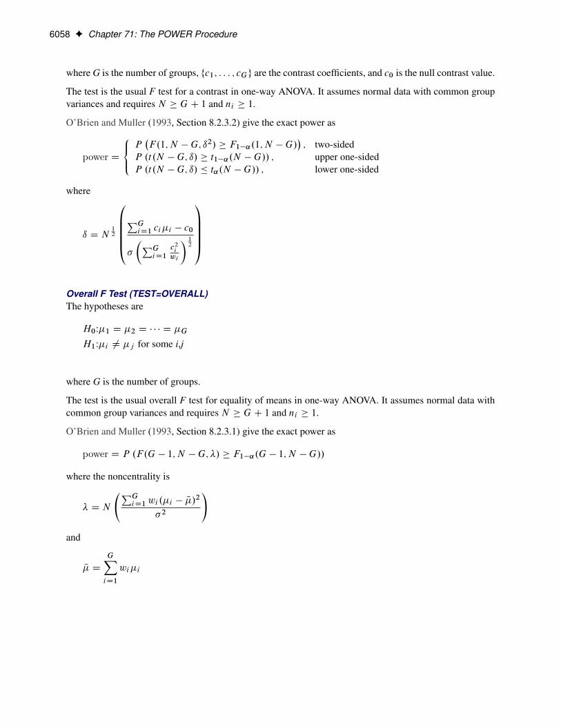
6058 F Chapter 71: The POWER Procedure
where G is the number of groups, fc1; : : : ; cGg are the contrast coefficients, and c0 is the null contrast value.
The test is the usual F test for a contrast in one-way ANOVA. It assumes normal data with common groupvariances and requires N � G C 1 and ni � 1.
O’Brien and Muller (1993, Section 8.2.3.2) give the exact power as
power D
8<:P�F.1;N �G; ı2/ � F1�˛.1;N �G/
�; two-sided
P .t.N �G; ı/ � t1�˛.N �G// ; upper one-sidedP .t.N �G; ı/ � t˛.N �G// ; lower one-sided
where
ı D N12
0BBBB@PGiD1 ci�i � c0
�
�PGiD1
c2i
wi
� 12
1CCCCA
Overall F Test (TEST=OVERALL)The hypotheses are
H0W�1 D �2 D � � � D �G
H1W�i ¤ �j for some i,j
where G is the number of groups.
The test is the usual overall F test for equality of means in one-way ANOVA. It assumes normal data withcommon group variances and requires N � G C 1 and ni � 1.
O’Brien and Muller (1993, Section 8.2.3.1) give the exact power as
power D P .F.G � 1;N �G; �/ � F1�˛.G � 1;N �G//
where the noncentrality is
� D N
PGiD1wi .�i � N�/
2
�2
!
and
N� D
GXiD1
wi�i

Computational Methods and Formulas F 6059
Analyses in the PAIREDFREQ Statement
Overview of Conditional McNemar testsNotation:
CaseFailure Success
Control Failure n00 n01 n0�Success n10 n11 n1�
n�0 n�1 N
n00 D #{control=failure, case=failure }
n01 D #{control=failure, case=success }
n10 D #{control=success, case=failure }
n11 D #{control=success, case=success }
N D n00 C n01 C n10 C n11
nD D n01 C n10 � # discordant pairs
O�ij Dnij
N
�ij D theoretical population value of O�ij�1� D �10 C �11
��1 D �01 C �11
� D Corr.control observation; case observation/ (within a pair)
DPR D “discordant proportion ratio” D�01
�10
DPR0 D null DPR
Power formulas are given here in terms of the discordant proportions �10 and �01. If the input is specifiedin terms of f�1�; ��1; �g, then it can be converted into values for f�10; �01g as follows:
�01 D ��1.1 � �1�/ � �..1 � �1�/�1�.1 � ��1/��1/12
�10 D �01 C �1� � ��1
All McNemar tests covered in PROC POWER are conditional, meaning that nD is assumed fixed at itsobserved value.
For the usual DPR0 D 1, the hypotheses are
H0W��1 D �1�
H1W
8<:��1 ¤ �1�; two-sided��1 > �1�; upper one-sided��1 < �1�; lower one-sided

6060 F Chapter 71: The POWER Procedure
The test statistic for both tests covered in PROC POWER (DIST=EXACT_COND and DIST=NORMAL)is the McNemar statistic QM , which has the following form when DPR0 D 1:
QM0 D.n01 � n10/
2
n01 C n10
For the conditional McNemar tests, this is equivalent to the square of the Z.X/ statistic for the test of asingle proportion (normal approximation to binomial), where the proportion is �01
�01C�10, the null is 0.5, and
“N” is nD (see, for example, Schork and Williams 1980):
Z.X/ Dn01 � nD.0:5/
ŒnD0:5.1 � 0:5/�12
�Ï N
0@n 12D. �01�01C�10
� 0:5/
Œ0:5.1 � 0:5/�12
;
�01�01C�10
�1 � �01
�01C�10
�0:5.1 � 0:5/
1AD
n01 � .n01 C n10/.0:5/
Œ.n01 C n10/0:5.1 � 0:5/�12
Dn01 � n10
Œn01 C n10�12
DpQM0
This can be generalized to a custom null for �01�01C�10
, which is equivalent to specifying a custom null DPR:
��01
�01 C �10
�0
�
264 1
1C 1�01�10
3750
�1
1C 1DPR0
So, a conditional McNemar test (asymptotic or exact) with a custom null is equivalent to the test of a singleproportion p1 � �01
�01C�10with a null value p0 � 1
1C 1DPR0
, with a sample size of nD:
H0Wp1 D p0
H1W
8<:p1 ¤ p0; two-sidedp1 > p0; one-sided Up1 < p0; one-sided L
which is equivalent to
H0WDPR D DPR0
H1W
8<:DPR ¤ DPR0; two-sidedDPR > DPR0; one-sided UDPR < DPR0; one-sided L
The general form of the test statistic is thus
QM D.n01 � nDp0/
2
nDp0.1 � p0/
The two most common conditional McNemar tests assume either the exact conditional distribution of QM(covered by the DIST=EXACT_COND analysis) or a standard normal distribution for QM (covered by theDIST=NORMAL analysis).

Computational Methods and Formulas F 6061
McNemar Exact Conditional Test (TEST=MCNEMAR DIST=EXACT_COND)For DIST=EXACT_COND, the power is calculated assuming that the test is conducted by using the exactconditional distribution of QM (conditional on nD). The power is calculated by first computing the con-ditional power for each possible nD . The unconditional power is computed as a weighted average over allpossible outcomes of nD:
power DNX
nDD0
P.nD/P.Reject p1 D p0jnD/
where nD Ï Bin.�01 C �10; N /, and P.Reject p1 D p0jnD/ is calculated by using the exact method inthe section “Exact Test of a Binomial Proportion (TEST=EXACT)” on page 6036.
The achieved significance level, reported as “Actual Alpha” in the analysis, is computed in the same wayexcept by using the actual alpha of the one-sample test in place of its power:
actual alpha DNX
nDD0
P.nD/˛?.p1; p0jnD/
where ˛?.p1; p0jnD/ is the actual alpha calculated by using the exact method in the section “Exact Test ofa Binomial Proportion (TEST=EXACT)” on page 6036 with proportion p1, null p0, and sample size nD .
McNemar Normal Approximation Test (TEST=MCNEMAR DIST=NORMAL)For DIST=NORMAL, power is calculated assuming the test is conducted by using the normal-approximatedistribution of QM (conditional on nD).
For the METHOD=EXACT option, the power is calculated in the same way as described in the section“McNemar Exact Conditional Test (TEST=MCNEMAR DIST=EXACT_COND)” on page 6061, exceptthat P.Reject p1 D p0jnD/ is calculated by using the exact method in the section “z Test for BinomialProportion Using Null Variance (TEST=Z VAREST=NULL)” on page 6037. The achieved significancelevel is calculated in the same way as described at the end of the section “McNemar Exact Conditional Test(TEST=MCNEMAR DIST=EXACT_COND)” on page 6061.
For the METHOD=MIETTINEN option, approximate sample size for the one-sided cases is computedaccording to equation (5.6) in Miettinen (1968):
N D
�z1�˛.p10 C p01/C zpower
�.p10 C p01/
2 �14.p01 � p10/
2.3C p10 C p01/� 12
�2.p10 C p01/.p01 � p10/2
Approximate power for the one-sided cases is computed by solving the sample size equation for power, andapproximate power for the two-sided case follows easily by summing the one-sided powers each at ˛=2:
power D
8̂̂̂̂ˆ̂̂̂̂̂̂ˆ̂̂<̂ˆ̂̂̂̂̂̂ˆ̂̂̂̂̂:
ˆ
.p01�p10/ŒN.p10Cp01/�
12�z1�˛.p10Cp01/
Œ.p10Cp01/2� 14 .p01�p10/2.3Cp10Cp01/�
12
!; upper one-sided
ˆ
�.p01�p10/ŒN.p10Cp01/�
12�z1�˛.p10Cp01/
Œ.p10Cp01/2� 14 .p01�p10/2.3Cp10Cp01/�
12
!; lower one-sided
ˆ
.p01�p10/ŒN.p10Cp01/�
12�z1�˛
2.p10Cp01/
Œ.p10Cp01/2� 14 .p01�p10/2.3Cp10Cp01/�
12
!C
ˆ
�.p01�p10/ŒN.p10Cp01/�
12�z1�˛
2.p10Cp01/
Œ.p10Cp01/2� 14 .p01�p10/2.3Cp10Cp01/�
12
!; two-sided

6062 F Chapter 71: The POWER Procedure
The two-sided solution for N is obtained by numerically inverting the power equation.
In general, compared to METHOD=CONNOR, the METHOD=MIETTINEN approximation tends to beslightly more accurate but can be slightly anticonservative in the sense of underestimating sample size andoverestimating power (Lachin 1992, p. 1250).
For the METHOD=CONNOR option, approximate sample size for the one-sided cases is computed accord-ing to equation (3) in Connor (1987):
N D
�z1�˛.p10 C p01/
12 C zpower
�p10 C p01 � .p01 � p10/
2� 12
�2.p01 � p10/2
Approximate power for the one-sided cases is computed by solving the sample size equation for power, andapproximate power for the two-sided case follows easily by summing the one-sided powers each at ˛=2:
power D
8̂̂̂̂ˆ̂̂̂̂̂̂ˆ̂̂<̂ˆ̂̂̂̂̂̂ˆ̂̂̂̂̂:
ˆ
.p01�p10/N
12�z1�˛.p10Cp01/
12
Œp10Cp01�.p01�p10/2�12
!; upper one-sided
ˆ
�.p01�p10/N
12�z1�˛.p10Cp01/
12
Œp10Cp01�.p01�p10/2�12
!; lower one-sided
ˆ
.p01�p10/N
12�z1�˛
2.p10Cp01/
12
Œp10Cp01�.p01�p10/2�12
!C
ˆ
�.p01�p10/N
12�z1�˛
2.p10Cp01/
12
Œp10Cp01�.p01�p10/2�12
!; two-sided
The two-sided solution for N is obtained by numerically inverting the power equation.
In general, compared to METHOD=MIETTINEN, the METHOD=CONNOR approximation tends to beslightly less accurate but slightly conservative in the sense of overestimating sample size and underestimat-ing power (Lachin 1992, p. 1250).
Analyses in the PAIREDMEANS Statement
Paired t Test (TEST=DIFF)The hypotheses for the paired t test are
H0W�diff D �0
H1W
8<:�diff ¤ �0; two-sided�diff > �0; upper one-sided�diff < �0; lower one-sided
The test assumes normally distributed data and requires N � 2. The test statistics are
t D N12
Nd � �0
sd
!Ï t .N � 1; ı/
t2 Ï F.1;N � 1; ı2/

Computational Methods and Formulas F 6063
where Nd and sd are the sample mean and standard deviation of the differences and
ı D N12
��diff � �0
�diff
�and
�diff D��21 C �
22 � 2��1�2
� 12
The test is
Reject H0 if
8<:t2 � F1�˛.1;N � 1/; two-sidedt � t1�˛.N � 1/; upper one-sidedt � t˛.N � 1/; lower one-sided
Exact power computations for t tests are given in O’Brien and Muller (1993, Section 8.2.2):
power D
8<:P�F.1;N � 1; ı2/ � F1�˛.1;N � 1/
�; two-sided
P .t.N � 1; ı/ � t1�˛.N � 1// ; upper one-sidedP .t.N � 1; ı/ � t˛.N � 1// ; lower one-sided
Paired t Test for Mean Ratio with Lognormal Data (TEST=RATIO)The lognormal case is handled by reexpressing the analysis equivalently as a normality-based test on thelog-transformed data, by using properties of the lognormal distribution as discussed in Johnson, Kotz, andBalakrishnan (1994, Chapter 14). The approaches in the section “Paired t Test (TEST=DIFF)” on page 6062then apply.
In contrast to the usual t test on normal data, the hypotheses with lognormal data are defined in terms ofgeometric means rather than arithmetic means.
The hypotheses for the paired t test with lognormal pairs fY1; Y2g are
H0W 2
1D 0
H1W
8̂<̂:
2 1¤ 0; two-sided
2 1> 0; upper one-sided
2 1< 0; lower one-sided
Let �?1 , �?2 , �?1 , �?2 , and �? be the (arithmetic) means, standard deviations, and correlation of the bivariatenormal distribution of the log-transformed data flog Y1; log Y2g. The hypotheses can be rewritten as follows:
H0W�?2 � �
?1 D log. 0/
H1W
8<:�?2 � �
?1 ¤ log. 0/; two-sided
�?2 � �?1 > log. 0/; upper one-sided
�?2 � �?1 < log. 0/; lower one-sided

6064 F Chapter 71: The POWER Procedure
where
�?1 D log 1�?2 D log 2
�?1 D�log.CV21 C 1/
� 12
�?2 D�log.CV22 C 1/
� 12
�? Dlog f�CV1CV2 C 1g
�?1 �?2
and CV1, CV2, and � are the coefficients of variation and the correlation of the original untransformed pairsfY1; Y2g. The conversion from � to �? is shown in Jones and Miller (1966).
The test assumes lognormally distributed data and requires N � 2. The power is
power D
8<:P�F.1;N � 1; ı2/ � F1�˛.1;N � 1/
�; two-sided
P .t.N � 1; ı/ � t1�˛.N � 1// ; upper one-sidedP .t.N � 1; ı/ � t˛.N � 1// ; lower one-sided
where
ı D N12
��?1 � �
?2 � log. 0/�?
�and
�? D��?21 C �
?22 � 2�
?�?1 �?2
� 12
Additive Equivalence Test for Mean Difference with Normal Data (TEST=EQUIV_DIFF)The hypotheses for the equivalence test are
H0W�diff < �L or �diff > �U
H1W�L � �diff � �U
The analysis is the two one-sided tests (TOST) procedure of Schuirmann (1987). The test assumes normallydistributed data and requires N � 2. Phillips (1990) derives an expression for the exact power assuming atwo-sample balanced design; the results are easily adapted to a paired design:
power D QN�1
.�t1�˛.N � 1//;
�diff � �U
�diffN� 12
I 0;.N � 1/
12 .�U � �L/
2�diffN� 12 .t1�˛.N � 1//
!�
QN�1
.t1�˛.N � 1//;
�diff � �L
�diffN� 12
I 0;.N � 1/
12 .�U � �L/
2�diffN� 12 .t1�˛.N � 1//
!where
�diff D��21 C �
22 � 2��1�2
� 12
and Q�.�; �I �; �/ is Owen’s Q function, defined in the section “Common Notation” on page 6027.

Computational Methods and Formulas F 6065
Multiplicative Equivalence Test for Mean Ratio with Lognormal Data (TEST=EQUIV_RATIO)The lognormal case is handled by reexpressing the analysis equivalently as a normality-based test on thelog-transformed data, by using properties of the lognormal distribution as discussed in Johnson, Kotz, andBalakrishnan (1994, Chapter 14). The approaches in the section “Additive Equivalence Test for MeanDifference with Normal Data (TEST=EQUIV_DIFF)” on page 6064 then apply.
In contrast to the additive equivalence test on normal data, the hypotheses with lognormal data are definedin terms of geometric means rather than arithmetic means.
The hypotheses for the equivalence test are
H0W T
R� �L or
T
R� �U
H1W�L < T
R< �U
where 0 < �L < �U
The analysis is the two one-sided tests (TOST) procedure of Schuirmann (1987) on the log-transformeddata. The test assumes lognormally distributed data and requires N � 2. Diletti, Hauschke, and Steinijans(1991) derive an expression for the exact power assuming a crossover design; the results are easily adaptedto a paired design:
power D QN�1
0@.�t1�˛.N � 1//; log� T R
�� log.�U /
�?N�12
I 0;.N � 1/
12 .log.�U / � log.�L//
2�?N�12 .t1�˛.N � 1//
1A�QN�1
[email protected]�˛.N � 1//; log� T R
�� log.�L/
�?N�12
I 0;.N � 1/
12 .log.�U / � log.�L//
2�?N�12 .t1�˛.N � 1//
1Awhere �? is the standard deviation of the differences between the log-transformed pairs (in other words,the standard deviation of log.YT / � log.YR/, where YT and YR are observations from the treatment andreference, respectively), computed as
�? D��?2R C �
?2T � 2�
?�?R�?T
� 12
�?R D�log.CV2R C 1/
� 12
�?T D�log.CV2T C 1/
� 12
�? Dlog f�CVRCVT C 1g
�?R�?T
where CVR, CVT , and � are the coefficients of variation and the correlation of the original untransformedpairs fYT ; YRg, and Q�.�; �I �; �/ is Owen’s Q function. The conversion from � to �? is shown in Jones andMiller (1966), and Owen’s Q function is defined in the section “Common Notation” on page 6027.
Confidence Interval for Mean Difference (CI=DIFF)This analysis of precision applies to the standard t-based confidence interval:h
Nd � t1�˛2.N � 1/ sdp
N; Nd C t1�˛
2.N � 1/ sdp
N
i; two-sidedh
Nd � t1�˛.N � 1/sdpN; 1
�; upper one-sided�
�1; Nd C t1�˛.N � 1/sdpN
i; lower one-sided

6066 F Chapter 71: The POWER Procedure
where Nd and sd are the sample mean and standard deviation of the differences. The “half-width” is definedas the distance from the point estimate Nd to a finite endpoint,
half-width D
(t1�˛
2.N � 1/ sdp
N; two-sided
t1�˛.N � 1/sdpN; one-sided
A “valid” conference interval captures the true mean difference. The exact probability of obtaining at mostthe target confidence interval half-width h, unconditional or conditional on validity, is given by Beal (1989):
Pr(half-width � h) D
8̂̂̂<̂ˆ̂:P
�2.N � 1/ � h2N.N�1/
�2diff.t2
1�˛2
.N�1//
!; two-sided
P
��2.N � 1/ � h2N.N�1/
�2diff.t21�˛.N�1//
�; one-sided
Pr(half-width � h |validity)
D
8̂<̂:�11�˛
�2hQN�1
�.t1�˛
2.N � 1//; 0I
0; b1/ �QN�1.0; 0I 0; b1/� ; two-sided�11�˛
�QN�1 ..t1�˛.N � 1//; 0I 0; b1/ ; one-sided
where
�diff D��21 C �
22 � 2��1�2
� 12
b1 Dh.N � 1/
12
�diff.t1�˛c.N � 1//N�
12
c D number of sides
and Q�.�; �I �; �/ is Owen’s Q function, defined in the section “Common Notation” on page 6027.
A “quality” confidence interval is both sufficiently narrow (half-width � h) and valid:
Pr(quality) D Pr(half-width � h and validity)
D Pr(half-width � h | validity)(1 � ˛)
Analyses in the TWOSAMPLEFREQ Statement
Overview of the 2 � 2 TableNotation:
OutcomeFailure Success
Group 1 n1 � x1 x1 n12 n2 � x2 x2 n2
N �m m N
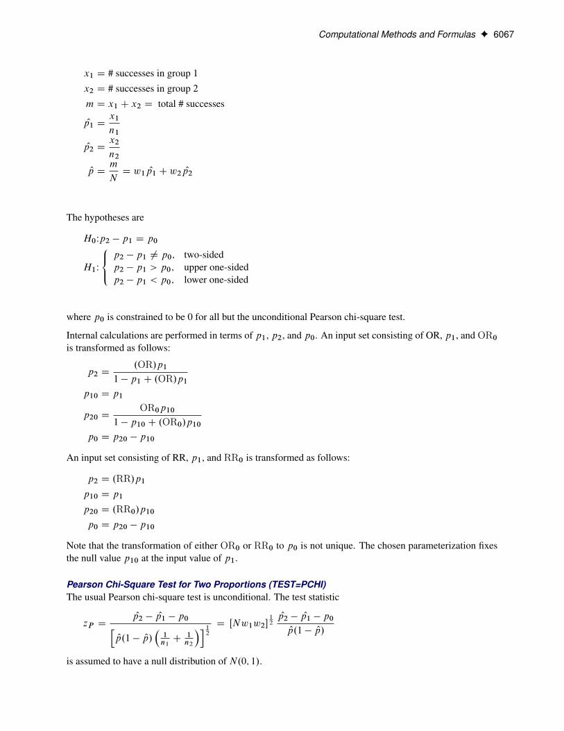
Computational Methods and Formulas F 6067
x1 D # successes in group 1
x2 D # successes in group 2
m D x1 C x2 D total # successes
Op1 Dx1
n1
Op2 Dx2
n2
Op Dm
ND w1 Op1 C w2 Op2
The hypotheses are
H0Wp2 � p1 D p0
H1W
8<:p2 � p1 ¤ p0; two-sidedp2 � p1 > p0; upper one-sidedp2 � p1 < p0; lower one-sided
where p0 is constrained to be 0 for all but the unconditional Pearson chi-square test.
Internal calculations are performed in terms of p1, p2, and p0. An input set consisting of OR, p1, and OR0is transformed as follows:
p2 D.OR/p1
1 � p1 C .OR/p1p10 D p1
p20 DOR0p10
1 � p10 C .OR0/p10p0 D p20 � p10
An input set consisting of RR, p1, and RR0 is transformed as follows:
p2 D .RR/p1p10 D p1
p20 D .RR0/p10p0 D p20 � p10
Note that the transformation of either OR0 or RR0 to p0 is not unique. The chosen parameterization fixesthe null value p10 at the input value of p1.
Pearson Chi-Square Test for Two Proportions (TEST=PCHI)The usual Pearson chi-square test is unconditional. The test statistic
zP DOp2 � Op1 � p0h
Op.1 � Op/�1n1C
1n2
�i 12
D ŒNw1w2�12Op2 � Op1 � p0
Op.1 � Op/
is assumed to have a null distribution of N.0; 1/.

6068 F Chapter 71: The POWER Procedure
Sample size for the one-sided cases is given by equation (4) in Fleiss, Tytun, and Ury (1980). One-sidedpower is computed as suggested by Diegert and Diegert (1981) by inverting the sample size formula. Powerfor the two-sided case is computed by adding the lower-sided and upper-sided powers each with ˛=2, andsample size for the two-sided case is obtained by numerically inverting the power formula. A custom nullvalue p0 for the proportion difference p2 � p1 is also supported.
power D
8̂̂̂̂ˆ̂̂̂̂̂̂<̂̂ˆ̂̂̂̂̂̂ˆ̂̂̂:
ˆ
�.p2�p1�p0/.Nw1w2/
12�z1�˛Œ.w1p1Cw2p2/.1�w1p1�w2p2/�
12
Œw2p1.1�p1/Cw1p2.1�p2/�12
�; upper one-sided
ˆ
��.p2�p1�p0/.Nw1w2/
12�z1�˛Œ.w1p1Cw2p2/.1�w1p1�w2p2/�
12
Œw2p1.1�p1/Cw1p2.1�p2/�12
�; lower one-sided
ˆ
.p2�p1�p0/.Nw1w2/
12�z1�˛
2Œ.w1p1Cw2p2/.1�w1p1�w2p2/�
12
Œw2p1.1�p1/Cw1p2.1�p2/�12
!C
ˆ
�.p2�p1�p0/.Nw1w2/
12�z1�˛
2Œ.w1p1Cw2p2/.1�w1p1�w2p2/�
12
Œw2p1.1�p1/Cw1p2.1�p2/�12
!; two-sided
For the one-sided cases, a closed-form inversion of the power equation yield an approximate total samplesize
N D
hz1�˛ f.w1p1 C w2p2/.1 � w1p1 � w2p2/g
12 C zpower fw2p1.1 � p1/C w1p2.1 � p2/g
12
i2w1w2.p2 � p1 � p0/2
For the two-sided case, the solution for N is obtained by numerically inverting the power equation.
Likelihood Ratio Chi-Square Test for Two Proportions (TEST=LRCHI)The usual likelihood ratio chi-square test is unconditional. The test statistic
zLR D .�1fp2<p1g/
vuut2N
2XiD1
�wi Opi log
�Opi
Op
�C wi .1 � Opi / log
�1 � Opi
1 � Op
��is assumed to have a null distribution of N.0; 1/ and an alternative distribution of N.ı; 1/, where
ı D N12 .�1fp2<p1g/
vuut2
2XiD1
�wipi log
�pi
w1p1 C w2p2
�C wi .1 � pi / log
�1 � pi
1 � .w1p1 C w2p2/
��The approximate power is
power D
8̂<̂:ˆ.ı � z1�˛/ ; upper one-sidedˆ.�ı � z1�˛/ ; lower one-sided
ˆ�ı � z1�˛
2
�Cˆ
��ı � z1�˛
2
�; two-sided
For the one-sided cases, a closed-form inversion of the power equation yield an approximate total samplesize
N D
�zpower C z1�˛
ı
�2For the two-sided case, the solution for N is obtained by numerically inverting the power equation.

Computational Methods and Formulas F 6069
Fisher’s Exact Conditional Test for Two Proportions (Test=FISHER)Fisher’s exact test is conditional on the observed total number of successes m. Power and sample sizecomputations are based on a test with similar power properties, the continuity-adjusted arcsine test. The teststatistic
zA D .4Nw1w2/12
"arcsin
�Op2 C
1
2Nw2.1f Op2< Op1g � 1f Op2> Op1g/
� 12
!
�arcsin
�Op1 C
1
2Nw1.1f Op1< Op2g � 1f Op1> Op2g/
� 12
!#
is assumed to have a null distribution of N.0; 1/ and an alternative distribution of N.ı; 1/, where
ı D .4Nw1w2/12
"arcsin
�p2 C
1
2Nw2.1fp2<p1g � 1fp2>p1g/
� 12
!
�arcsin
�p1 C
1
2Nw1.1fp1<p2g � 1fp1>p2g/
� 12
!#
The approximate power for the one-sided balanced case is given by Walters (1979) and is easily extendedto the unbalanced and two-sided cases:
power D
8̂<̂:ˆ.ı � z1�˛/ ; upper one-sidedˆ.�ı � z1�˛/ ; lower one-sided
ˆ�ı � z1�˛
2
�Cˆ
��ı � z1�˛
2
�; two-sided
Analyses in the TWOSAMPLEMEANS Statement
Two-Sample t Test Assuming Equal Variances (TEST=DIFF)The hypotheses for the two-sample t test are
H0W�diff D �0
H1W
8<:�diff ¤ �0; two-sided�diff > �0; upper one-sided�diff < �0; lower one-sided
The test assumes normally distributed data and common standard deviation per group, and it requiresN � 3,n1 � 1, and n2 � 1. The test statistics are
t D N12 .w1w2/
12
�Nx2 � Nx1 � �0
sp
�Ï t .N � 2; ı/
t2 Ï F.1;N � 2; ı2/
where Nx1 and Nx2 are the sample means and sp is the pooled standard deviation, and
ı D N12 .w1w2/
12
��diff � �0
�
�

6070 F Chapter 71: The POWER Procedure
The test is
Reject H0 if
8<:t2 � F1�˛.1;N � 2/; two-sidedt � t1�˛.N � 2/; upper one-sidedt � t˛.N � 2/; lower one-sided
Exact power computations for t tests are given in O’Brien and Muller (1993, Section 8.2.1):
power D
8<:P�F.1;N � 2; ı2/ � F1�˛.1;N � 2/
�; two-sided
P .t.N � 2; ı/ � t1�˛.N � 2// ; upper one-sidedP .t.N � 2; ı/ � t˛.N � 2// ; lower one-sided
Solutions for N, n1, n2, ˛, and ı are obtained by numerically inverting the power equation. Closed-formsolutions for other parameters, in terms of ı, are as follows:
�diff D ı�.Nw1w2/� 12 C �0
�1 D ı�.Nw1w2/� 12 C �0 � �2
�2 D ı�.Nw1w2/� 12 C �0 � �1
� D
(ı�1.Nw1w2/
12 .�diff � �0/; jıj > 0
undefined; otherwise
w1 D
8<: 12˙
12
h1 � 4ı2�2
N.�diff��0/2
i 12; 0 < jıj � 1
2N12j�diff��0j
�
undefined; otherwise
w2 D
8<: 12˙
12
h1 � 4ı2�2
N.�diff��0/2
i 12; 0 < jıj � 1
2N12j�diff��0j
�
undefined; otherwise
Finally, here is a derivation of the solution for w1:
Solve the ı equation for w1 (which requires the quadratic formula). Then determine the range of ı givenw1:
minw1.ı/ D
(0; when w1 D 0 or 1; if .�diff � �0/ � 012N12.�diff��0/
�; when w1 D
12; if .�diff � �0/ < 0
maxw1
.ı/ D
(0; when w1 D 0 or 1; if .�diff � �0/ < 012N12.�diff��0/
�; when w1 D
12; if .�diff � �0/ � 0
This implies
jıj �1
2N12j�diff � �0j
�

Computational Methods and Formulas F 6071
Two-Sample Satterthwaite t Test Assuming Unequal Variances (TEST=DIFF_SATT)The hypotheses for the two-sample Satterthwaite t test are
H0W�diff D �0
H1W
8<:�diff ¤ �0; two-sided�diff > �0; upper one-sided�diff < �0; lower one-sided
The test assumes normally distributed data and requires N � 3, n1 � 1, and n2 � 1. The test statistics are
t DNx2 � Nx1 � �0�s21n1C
s22n2
� 12
D N12Nx2 � Nx1 � �0�s21w1C
s22w2
� 12
F D t2
where Nx1 and Nx2 are the sample means and s1 and s2 are the sample standard deviations.
DiSantostefano and Muller (1995, p. 585) state, the test is based on assuming that underH0, F is distributedas F.1; �/, where � is given by Satterthwaite’s approximation (Satterthwaite 1946),
� D
��21n1C
�22n2
�2��21n1
�2n1�1
C
��22n2
�2n2�1
D
��21w1C
�22w2
�2��21w1
�2Nw1�1
C
��22w2
�2Nw2�1
Since � is unknown, in practice it must be replaced by an estimate
O� D
�s21n1C
s22n2
�2�s21n1
�2n1�1
C
�s22n2
�2n2�1
D
�s21w1C
s22w2
�2�s21w1
�2Nw1�1
C
�s22w2
�2Nw2�1
So the test is
Reject H0 if
8<:F � F1�˛.1; O�/; two-sidedt � t1�˛. O�/; upper one-sidedt � t˛. O�/; lower one-sided
Exact solutions for power for the two-sided and upper one-sided cases are given in Moser, Stevens, andWatts (1989). The lower one-sided case follows easily by using symmetry. The equations are as follows:

6072 F Chapter 71: The POWER Procedure
power D
8̂̂̂̂ˆ̂̂̂̂̂<̂ˆ̂̂̂̂̂̂ˆ̂:
R10 P .F.1;N � 2; �/ >
h.u/F1�˛.1; v.u//ju/ f .u/du; two-sidedR10 P
�t .N � 2; �
12 / >
Œh.u/�12 t1�˛.v.u//ju
�f .u/du; upper one-sidedR1
0 P�t .N � 2; �
12 / <
Œh.u/�12 t˛.v.u//ju
�f .u/du; lower one-sided
where
h.u/ D
�1n1C
un2
�.n1 C n2 � 2/�
.n1 � 1/C .n2 � 1/u�21�22
��1n1C
�22�21n2
�
v.u/ D
�1n1C
un2
�21
n21.n1�1/C
u2
n22.n2�1/
� D.�diff � �0/
2
�21n1C
�22n2
f .u/ D��n1Cn2�2
2
���n1�12
���n2�12
� "�21 .n2 � 1/�22 .n1 � 1/
#n2�12
un2�3
2
"1C
�n2 � 1
n1 � 1
�u�21
�22
#��n1Cn2�22
�
The density f .u/ is obtained from the fact that
u�21
�22� F.n2 � 1; n1 � 1/
Two-Sample Pooled t Test of Mean Ratio with Lognormal Data (TEST=RATIO)The lognormal case is handled by reexpressing the analysis equivalently as a normality-based test on thelog-transformed data, by using properties of the lognormal distribution as discussed in Johnson, Kotz, andBalakrishnan (1994, Chapter 14). The approaches in the section “Two-Sample t Test Assuming EqualVariances (TEST=DIFF)” on page 6069 then apply.
In contrast to the usual t test on normal data, the hypotheses with lognormal data are defined in terms ofgeometric means rather than arithmetic means. The test assumes equal coefficients of variation in the twogroups.
The hypotheses for the two-sample t test with lognormal data are
H0W 2
1D 0
H1W
8̂<̂:
2 1¤ 0; two-sided
2 1> 0; upper one-sided
2 1< 0; lower one-sided

Computational Methods and Formulas F 6073
Let �?1 , �?2 , and �? be the (arithmetic) means and common standard deviation of the corresponding normaldistributions of the log-transformed data. The hypotheses can be rewritten as follows:
H0W�?2 � �
?1 D log. 0/
H1W
8<:�?2 � �
?1 ¤ log. 0/; two-sided
�?2 � �?1 > log. 0/; upper one-sided
�?2 � �?1 < log. 0/; lower one-sided
where
�?1 D log 1�?2 D log 2
The test assumes lognormally distributed data and requires N � 3, n1 � 1, and n2 � 1.
The power is
power D
8<:P�F.1;N � 2; ı2/ � F1�˛.1;N � 2/
�; two-sided
P .t.N � 2; ı/ � t1�˛.N � 2// ; upper one-sidedP .t.N � 2; ı/ � t˛.N � 2// ; lower one-sided
where
ı D N12 .w1w2/
12
��?2 � �
?1 � log. 0/�?
��? D
�log.CV2 C 1/
� 12
Additive Equivalence Test for Mean Difference with Normal Data (TEST=EQUIV_DIFF)The hypotheses for the equivalence test are
H0W�diff < �L or �diff > �U
H1W�L � �diff � �U
The analysis is the two one-sided tests (TOST) procedure of Schuirmann (1987). The test assumes normallydistributed data and requires N � 3, n1 � 1, and n2 � 1. Phillips (1990) derives an expression for theexact power assuming a balanced design; the results are easily adapted to an unbalanced design:
power D QN�2
.�t1�˛.N � 2//;
�diff � �U
�N�12 .w1w2/
� 12
I 0;.N � 2/
12 .�U � �L/
2�N�12 .w1w2/
� 12 .t1�˛.N � 2//
!�
QN�2
.t1�˛.N � 2//;
�diff � �L
�N�12 .w1w2/
� 12
I 0;.N � 2/
12 .�U � �L/
2�N�12 .w1w2/
� 12 .t1�˛.N � 2//
!
where Q�.�; �I �; �/ is Owen’s Q function, defined in the section “Common Notation” on page 6027.
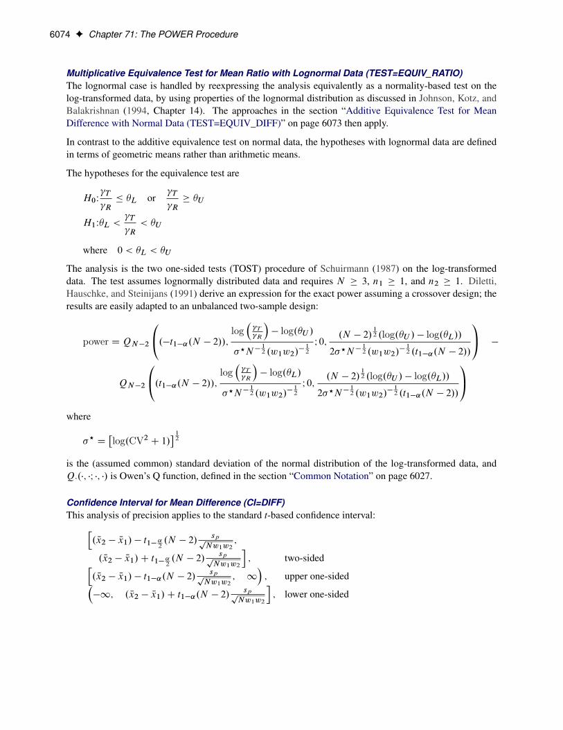
6074 F Chapter 71: The POWER Procedure
Multiplicative Equivalence Test for Mean Ratio with Lognormal Data (TEST=EQUIV_RATIO)The lognormal case is handled by reexpressing the analysis equivalently as a normality-based test on thelog-transformed data, by using properties of the lognormal distribution as discussed in Johnson, Kotz, andBalakrishnan (1994, Chapter 14). The approaches in the section “Additive Equivalence Test for MeanDifference with Normal Data (TEST=EQUIV_DIFF)” on page 6073 then apply.
In contrast to the additive equivalence test on normal data, the hypotheses with lognormal data are definedin terms of geometric means rather than arithmetic means.
The hypotheses for the equivalence test are
H0W T
R� �L or
T
R� �U
H1W�L < T
R< �U
where 0 < �L < �U
The analysis is the two one-sided tests (TOST) procedure of Schuirmann (1987) on the log-transformeddata. The test assumes lognormally distributed data and requires N � 3, n1 � 1, and n2 � 1. Diletti,Hauschke, and Steinijans (1991) derive an expression for the exact power assuming a crossover design; theresults are easily adapted to an unbalanced two-sample design:
power D QN�2
0@.�t1�˛.N � 2//; log� T R
�� log.�U /
�?N�12 .w1w2/
� 12
I 0;.N � 2/
12 .log.�U / � log.�L//
2�?N�12 .w1w2/
� 12 .t1�˛.N � 2//
1A �
QN�2
[email protected]�˛.N � 2//; log� T R
�� log.�L/
�?N�12 .w1w2/
� 12
I 0;.N � 2/
12 .log.�U / � log.�L//
2�?N�12 .w1w2/
� 12 .t1�˛.N � 2//
1Awhere
�? D�log.CV2 C 1/
� 12
is the (assumed common) standard deviation of the normal distribution of the log-transformed data, andQ�.�; �I �; �/ is Owen’s Q function, defined in the section “Common Notation” on page 6027.
Confidence Interval for Mean Difference (CI=DIFF)This analysis of precision applies to the standard t-based confidence interval:h
. Nx2 � Nx1/ � t1�˛2.N � 2/
sppNw1w2
;
. Nx2 � Nx1/C t1�˛2.N � 2/
sppNw1w2
i; two-sidedh
. Nx2 � Nx1/ � t1�˛.N � 2/sppNw1w2
; 1�; upper one-sided�
�1; . Nx2 � Nx1/C t1�˛.N � 2/sppNw1w2
i; lower one-sided

Computational Methods and Formulas F 6075
where Nx1 and Nx2 are the sample means and sp is the pooled standard deviation. The “half-width” is definedas the distance from the point estimate Nx2 � Nx1 to a finite endpoint,
half-width D
(t1�˛
2.N � 2/
sppNw1w2
; two-sidedt1�˛.N � 2/
sppNw1w2
; one-sided
A “valid” conference interval captures the true mean. The exact probability of obtaining at most the targetconfidence interval half-width h, unconditional or conditional on validity, is given by Beal (1989):
Pr(half-width � h) D
8̂̂̂<̂ˆ̂:P
�2.N � 2/ � h2N.N�2/.w1w2/
�2.t21�˛
2
.N�2//
!; two-sided
P
��2.N � 2/ � h2N.N�2/.w1w2/
�2.t21�˛.N�2//
�; one-sided
Pr(half-width � h |validity)
D
8̂<̂:�11�˛
�2hQN�2
�.t1�˛
2.N � 2//; 0I
0; b2/ �QN�2.0; 0I 0; b2/� ; two-sided�11�˛
�QN�2 ..t1�˛.N � 2//; 0I 0; b2/ ; one-sided
where
b2 Dh.N � 2/
12
�.t1�˛c.N � 2//N�
12 .w1w2/
� 12
c D number of sides
and Q�.�; �I �; �/ is Owen’s Q function, defined in the section “Common Notation” on page 6027.
A “quality” confidence interval is both sufficiently narrow (half-width � h) and valid:
Pr(quality) D Pr(half-width � h and validity)
D Pr(half-width � h | validity)(1 � ˛)
Analyses in the TWOSAMPLESURVIVAL Statement
Rank Tests for Two Survival Curves (TEST=LOGRANK, TEST=GEHAN, TEST=TARONEWARE)The method is from Lakatos (1988) and Cantor (1997, pp. 83–92).

6076 F Chapter 71: The POWER Procedure
Define the following notation:
Xj .i/ D ith input time point on survival curve for group j
Sj .i/ D input survivor function value corresponding to Xj .i/
hj .t/ D hazard rate for group j at time t
‰j .t/ D loss hazard rate for group j at time t
�j D exponential hazard rate for group j
R D hazard ratio of group 2 to group 1� (assumed constant) value of h2.t/h1.t/
mj D median survival time for group j
b D number of subintervals per time unit
T D accrual time
� D follow-up time after accrual
Lj D exponential loss rate for group j
XLj D input time point on loss curve for group j
SLj D input survivor function value corresponding to XLjmLj D median survival time for group j
ri D rank for ith time point
Each survival curve can be specified in one of several ways.
� For exponential curves:
– a single point .Xj .1/; Sj .1// on the curve
– median survival time
– hazard rate
– hazard ratio (for curve 2, with respect to curve 1)
� For piecewise linear curves with proportional hazards:
– a set of points f.X1.1/; S1.1//; .X1.2/; S1.2//; : : :g (for curve 1)
– hazard ratio (for curve 2, with respect to curve 1)
� For arbitrary piecewise linear curves:
– a set of points f.Xj .1/; Sj .1//; .Xj .2/; Sj .2//; : : :g
A total ofM C1 evenly spaced time points ft0 D 0; t1; t2; : : : ; tM D T C�g are used in calculations, where
M D floor ..T C �/b/

Computational Methods and Formulas F 6077
The hazard function is calculated for each survival curve at each time point. For an exponential curve, the(constant) hazard is given by one of the following, depending on the input parameterization:
hj .t/ D
8̂̂̂̂ˆ̂<̂ˆ̂̂̂̂:
�j�1R� log. 1
2/
mj� log.Sj .1//Xj .1/
� log.S1.1//X1.1/
R
For a piecewise linear curve, define the following additional notation:
t�i D largest input time X such that X � titCi D smallest input time X such that X > ti
The hazard is computed by using linear interpolation as follows:
hj .ti / DSj .t
�i / � Sj .t
Ci /�
Sj .tCi / � Sj .t
�i /� �ti � t
�i
�C Sj .t
�i /�tCi � t
�i
�With proportional hazards, the hazard rate of group 2’s curve in terms of the hazard rate of group 1’s curveis
h2.t/ D h1.t/R
Hazard function values f‰j .ti /g for the loss curves are computed in an analogous way fromfLj ; XLj ; SLj ; mLj g.
The expected number at riskNj .i/ at time i in group j is calculated for each group and time points 0 throughM – 1, as follows:
Nj .0/ D Nwj
Nj .i C 1/ D Nj .i/
�1 � hj .ti /
�1
b
��‰j .ti /
�1
b
��
�1
b.T C � � ti /
�1fti>�g
�
Define �i as the ratio of hazards and �i as the ratio of expected numbers at risk for time ti :
�i Dh2.ti /
h1.ti /
�i DN2.i/
N1.i/
The expected number of deaths in each subinterval is calculated as follows:
Di D Œh1.ti /N1.i/C h2.ti /N2.i/�
�1
b
�

6078 F Chapter 71: The POWER Procedure
The rank values are calculated as follows according to which test statistic is used:
ri D
8<:1; log-rankN1.i/CN2.i/; GehanpN1.i/CN2.i/; Tarone-Ware
The distribution of the test statistic is approximated by N.E; 1/ where
E D
PM�1iD0 Diri
h�i�i1C�i�i
��i1C�i
iqPM�1
iD0 Dir2i
�i.1C�i /2
Note that N12 can be factored out of the mean E, and so it can be expressed equivalently as
E D N12E? D N
12
264PM�1iD0 D?i r
?i
h�i�i1C�i�i
��i1C�i
iqPM�1
iD0 D?i r?i2 �i.1C�i /2
375where E? is free of N and
D?i D�h1.ti /N
?1 .i/C h2.ti /N
?2 .i/
� �1b
�
r?i D
8<:1; log-rankN ?1 .i/CN
?2 .i/; Gehanp
N ?1 .i/CN
?2 .i/; Tarone-Ware
N ?j .0/ D wj
N ?j .i C 1/ D N
?j .i/
�1 � hj .ti /
�1
b
��‰j .ti /
�1
b
��
�1
b.T C � � ti /
�1fti>�g
�
The approximate power is
power D
8̂̂̂<̂ˆ̂:ˆ��N
12E? � z1�˛
�; upper one-sided
ˆ�N12E? � z1�˛
�; lower one-sided
ˆ��N
12E? � z1�˛
2
�Cˆ
�N
12E? � z1�˛
2
�; two-sided
Note that the upper and lower one-sided cases are expressed differently than in other analyses. This isbecause E? > 0 corresponds to a higher survival curve in group 1 and thus, by the convention used inPROC power for two-group analyses, the lower side.
For the one-sided cases, a closed-form inversion of the power equation yield an approximate total samplesize
N D
�zpower C z1�˛
E?
�2For the two-sided case, the solution for N is obtained by numerically inverting the power equation.
Accrual rates are converted to and from sample sizes according to the equation aj D nj =T , where aj isthe accrual rate for group j.

Computational Methods and Formulas F 6079
Expected numbers of events—that is, deaths, whether observed or censored—are converted to and fromsample sizes according to the equation
ej D
(nj�1 � Sj .�/
�; T D 0
nj
h1 � 1
T
R T0 Sj .T C � � t /dt
i; T > 0
where ej is the expected number of events in group j. For an exponential curve, the equation simplifies to
ej D
(nj�1 � exp.��j �/
�; T D 0
nj
h1 � 1
�jT
�exp.��j �/ � exp.��j .T C �//
�i; T > 0
For a piecewise linear curve, first define Kj as the number of time points in the following collection: � ,T C � , and input time points for group j strictly between � and T C � . Denote the ordered set of these pointsas fuj1; : : : ; ujKj g. The survival function values Sj .�/ and Sj .T C�/ are calculated by linear interpolationbetween adjacent input time points if they do not coincide with any input time points. Then the equation fora piecewise linear curve simplifies to
ej D
(nj�1 � Sj .�/
�; T D 0
nj
h1 � 1
2T
PKj�1
iD1
�uj;iC1 � uj i
� �Sj .uj i /C Sj .uj;iC1/
�i; T > 0
Analyses in the TWOSAMPLEWILCOXON Statement
Wilcoxon-Mann-Whitney Test for Comparing Two Distributions (TEST=WMW)The power approximation in this section is applicable to the Wilcoxon-Mann-Whitney (WMW) test asinvoked with the WILCOXON option in the PROC NPAR1WAY statement of the NPAR1WAY procedure.The approximation is based on O’Brien and Castelloe (2006) and an estimator called 4WMWodds. SeeO’Brien and Castelloe (2006) for a definition of 4WMWodds, which need not be derived in detail here forpurposes of explaining the power formula.
Let Y1 and Y2 be independent observations from any two distributions that you want to compare using theWMW test. For purposes of deriving the asymptotic distribution of 4WMWodds (and consequently the powercomputation as well), these distributions must be formulated as ordered categorical (“ordinal”) distributions.
If a distribution is continuous, it can be discretized using a large number of categories with negligible lossof accuracy. Each nonordinal distribution is divided into b categories, where b is the value of the NBINSparameter, with breakpoints evenly spaced on the probability scale. That is, each bin contains an equalprobability 1/b for that distribution. Then the breakpoints across both distributions are pooled to form acollection of C bins (heretofore called “categories”), and the probabilities of bin membership for each dis-tribution are recalculated. The motivation for this method of binning is to avoid degenerate representationsof the distributions—that is, small handfuls of large probabilities among mostly empty bins—as can becaused by something like an evenly spaced grid across raw values rather than probabilities.
After the discretization process just mentioned, there are now two ordinal distributions, each with a set ofprobabilities across a common set of C ordered categories. For simplicity of notation, assume (without lossof generality) the response values to be 1; : : : ; C . Represent the conditional probabilities as
Qpij D Prob .Yi D j j group D i/ ; i 2 f1; 2g and j 2 f1; : : : ; C g
and the group allocation weights as
wi Dni
ND Prob .group D i/ ; i 2 f1; 2g

6080 F Chapter 71: The POWER Procedure
The joint probabilities can then be calculated simply as
pij D Prob .group D i; Yi D j / D wi Qpij ; i 2 f1; 2g and j 2 f1; : : : ; C g
The next step in the power computation is to compute the probabilities that a randomly chosen pair ofobservations from the two groups is concordant, discordant, or tied. It is useful to define these probabilitiesas functions of the terms Rsij and Rdij , defined as follows, where Y is a random observation drawn fromthe joint distribution across groups and categories:
Rsij D Prob .Y is concordant with cell.i; j //C1
2Prob .Y is tied with cell.i; j //
D Prob ..group < i and Y < j / or .group > i and Y > j //C1
2Prob .group ¤ i and Y D j /
D
2XgD1
CXcD1
wg Qpgc
�I.g�i/.c�j />0 C
1
2Ig¤i;cDj
�and
Rdij D Prob .Y is discordant with cell.i; j //C1
2Prob .Y is tied with cell.i; j //
D Prob ..group < i and Y > j / or .group > i and Y < j //C1
2Prob .group ¤ i and Y D j /
D
2XgD1
CXcD1
wg Qpgc
�I.g�i/.c�j /<0 C
1
2Ig¤i;cDj
�
For an independent random draw Y1; Y2 from the two distributions,
Pc D Prob .Y1; Y2 concordant/C1
2Prob .Y1; Y2 tied/
D
2XiD1
CXjD1
wi QpijRsij
and
Pd D Prob .Y1; Y2 discordant/C1
2Prob .Y1; Y2 tied/
D
2XiD1
CXjD1
wi QpijRdij
Then
WMWodds DPc
Pd

ODS Graphics F 6081
Proceeding to compute the theoretical standard error associated with WMWodds (that is, the populationanalogue to the sample standard error),
SE.WMWodds/ D2
Pd
24 2XiD1
CXjD1
wi Qpij�WMWoddsRdij �Rsij
�2=N
35 12
Converting to the natural log scale and using the delta method,
SE.log.WMWodds// DSE.WMWodds/
WMWodds
The next step is to produce a “smoothed” version of the 2 � C cell probabilities that conforms to the nullhypothesis of the Wilcoxon-Mann-Whitney test (in other words, independence in the 2 � C contingencytable of probabilities). Let SEH0.log.WMWodds// denote the theoretical standard error of log.WMWodds/
assuming H0.
Finally we have all of the terms needed to compute the power, using the noncentral chi-square and normaldistributions:
power D
8̂̂̂̂<̂ˆ̂̂:P�Z �
SEH0 .log.WMWodds//
SE.log.WMWodds//z1�˛ � ı
?N12
�; upper one-sided
P�Z �
SEH0 .log.WMWodds//
SE.log.WMWodds//z˛ � ı
?N12
�; lower one-sided
P
��2.1; .ı?/2N/ �
hSEH0 .log.WMWodds//
SE.log.WMWodds//
i2�21�˛.1/
�; two-sided
where
ı? Dlog.WMWodds/
N12SE.log.WMWodds//
is the primary noncentrality—that is, the “effect size” that quantifies how much the two conjectured distri-butions differ. Z is a standard normal random variable, �2.df ;nc/ is a noncentral �2 random variable withdegrees of freedom df and noncentrality nc, and N is the total sample size.
ODS GraphicsStatistical procedures use ODS Graphics to create graphs as part of their output. ODS Graphics is describedin detail in Chapter 21, “Statistical Graphics Using ODS.”
Before you create graphs, ODS Graphics must be enabled (for example, by specifying the ODS GRAPHICSON statement). For more information about enabling and disabling ODS Graphics, see the section “Enablingand Disabling ODS Graphics” on page 600 in Chapter 21, “Statistical Graphics Using ODS.”
The overall appearance of graphs is controlled by ODS styles. Styles and other aspects of using ODSGraphics are discussed in the section “A Primer on ODS Statistical Graphics” on page 599 in Chapter 21,“Statistical Graphics Using ODS.”
If ODS Graphics is not enabled, then PROC POWER creates traditional graphics.

6082 F Chapter 71: The POWER Procedure
You can reference every graph produced through ODS Graphics with a name. The names of the graphs thatPROC POWER generates are listed in Table 71.31, along with the required statements and options.
Table 71.31 Graphs Produced by PROC POWER
ODS Graph Name Plot Description Option
PowerPlot Plot with two of the following three parameters on theX and Y axes: power, sample size, and effect size
PLOT
PowerAbort Empty plot that shows an error message when a plotcould not be produced
PLOT
ODS Styles Suitable for Use with PROC POWERODS styles control the appearance of graphs produced by PROC POWER. ODS provides over 50 styles,but most are not suitable for use in PROC POWER. PROC POWER requires a style that distinguishescurves based on a combination of color, line style, and symbol marker. Styles that are well-suited for use inPROC POWER include: STATISTICAL, ANALYSIS, DEFAULT, LISTING, and HTMLBLUECML. TheHTMLBLUE and PLATEAU styles are commonly used, but they are not well-suited for use with PROCPOWER because they rely primarily on color to distinguish curves rather than a combination of color, linestyle, and symbol marker.
In this chapter, a style is explicitly specified at the start of each example that uses ODS Graphics to remindyou to use one of the suitable styles. Styles are specified in an ODS destination statement. Destinationsinclude LISTING, HTML, RTF, PDF, and many others. You can set the style and the destination as follows:
ods html style=htmlbluecml;ods graphics on;
proc power;onesamplemeans
mean = 5 10ntotal = 150stddev = 30 50power = .;
plot x=n min=100 max=200;run;
ods graphics off;ods html close;
For more information about ODS and ODS destinations, see Chapter 20, “Using the Output Delivery Sys-tem.” For more information ODS styles, see Chapter 21, “Statistical Graphics Using ODS.”

Examples: POWER Procedure F 6083
Examples: POWER Procedure
Example 71.1: One-Way ANOVAThis example deals with the same situation as in Example 44.1 of Chapter 44, “The GLMPOWER Proce-dure.”
Hocking (1985, p. 109) describes a study of the effectiveness of electrolytes in reducing lactic acid buildupfor long-distance runners. You are planning a similar study in which you will allocate five different fluids torunners on a 10-mile course and measure lactic acid buildup immediately after the run. The fluids consist ofwater and two commercial electrolyte drinks, EZDure and LactoZap, each prepared at two concentrations,low (EZD1 and LZ1) and high (EZD2 and LZ2).
You conjecture that the standard deviation of lactic acid measurements given any particular fluid is about3.75, and that the expected lactic acid values will correspond roughly to those in Table 71.32. You are leastfamiliar with the LZ1 drink and hence decide to consider a range of reasonable values for that mean.
Table 71.32 Mean Lactic Acid Buildup by Fluid
Water EZD1 EZD2 LZ1 LZ2
35.6 33.7 30.2 29 or 28 25.9
You are interested in four different comparisons, shown in Table 71.33 with appropriate contrast coefficients.
Table 71.33 Planned Comparisons
Contrast CoefficientsComparison Water EZD1 EZD2 LZ1 LZ2Water versus electrolytes 4 –1 –1 –1 –1EZD versus LZ 0 1 1 –1 –1EZD1 versus EZD2 0 1 –1 0 0LZ1 versus LZ2 0 0 0 1 –1
For each of these contrasts you want to determine the sample size required to achieve a power of 0.9 fordetecting an effect with magnitude in accord with Table 71.32. You are not yet attempting to choose a singlesample size for the study, but rather checking the range of sample sizes needed for individual contrasts. Youplan to test each contrast at ˛ D 0:025. In the interests of reducing costs, you will provide twice as manyrunners with water as with any of the electrolytes; in other words, you will use a sample size weightingscheme of 2:1:1:1:1. Use the ONEWAYANOVA statement in the POWER procedure to compute the samplesizes.
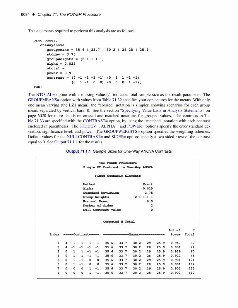
6084 F Chapter 71: The POWER Procedure
The statements required to perform this analysis are as follows:
proc power;onewayanova
groupmeans = 35.6 | 33.7 | 30.2 | 29 28 | 25.9stddev = 3.75groupweights = (2 1 1 1 1)alpha = 0.025ntotal = .power = 0.9contrast = (4 -1 -1 -1 -1) (0 1 1 -1 -1)
(0 1 -1 0 0) (0 0 0 1 -1);run;
The NTOTAL= option with a missing value (.) indicates total sample size as the result parameter. TheGROUPMEANS= option with values from Table 71.32 specifies your conjectures for the means. With onlyone mean varying (the LZ1 mean), the “crossed” notation is simpler, showing scenarios for each groupmean, separated by vertical bars (|). See the section “Specifying Value Lists in Analysis Statements” onpage 6020 for more details on crossed and matched notations for grouped values. The contrasts in Ta-ble 71.33 are specified with the CONTRAST= option, by using the “matched” notation with each contrastenclosed in parentheses. The STDDEV=, ALPHA=, and POWER= options specify the error standard de-viation, significance level, and power. The GROUPWEIGHTS= option specifies the weighting schemes.Default values for the NULLCONTRAST= and SIDES= options specify a two-sided t test of the contrastequal to 0. See Output 71.1.1 for the results.
Output 71.1.1 Sample Sizes for One-Way ANOVA Contrasts
The POWER ProcedureSingle DF Contrast in One-Way ANOVA
Fixed Scenario Elements
Method ExactAlpha 0.025Standard Deviation 3.75Group Weights 2 1 1 1 1Nominal Power 0.9Number of Sides 2Null Contrast Value 0
Computed N Total
Actual NIndex -----Contrast----- -------------Means------------- Power Total
1 4 -1 -1 -1 -1 35.6 33.7 30.2 29 25.9 0.947 302 4 -1 -1 -1 -1 35.6 33.7 30.2 28 25.9 0.901 243 0 1 1 -1 -1 35.6 33.7 30.2 29 25.9 0.929 604 0 1 1 -1 -1 35.6 33.7 30.2 28 25.9 0.922 485 0 1 -1 0 0 35.6 33.7 30.2 29 25.9 0.901 1746 0 1 -1 0 0 35.6 33.7 30.2 28 25.9 0.901 1747 0 0 0 1 -1 35.6 33.7 30.2 29 25.9 0.902 2228 0 0 0 1 -1 35.6 33.7 30.2 28 25.9 0.902 480
Example 71.1: One-Way ANOVA F 6085
The sample sizes in Output 71.1.1 range from 24 for the comparison of water versus electrolytes to 480 forthe comparison of LZ1 versus LZ2, both assuming the smaller LZ1 mean. The sample size for the lattercomparison is relatively large because the small mean difference of 28 � 25:9 D 2:1 is hard to detect.
The Nominal Power of 0.9 in the “Fixed Scenario Elements” table in Output 71.1.1 represents the inputtarget power, and the Actual Power column in the “Computed N Total” table is the power at the sample size(N Total) adjusted to achieve the specified sample weighting. Note that all of the sample sizes are roundedup to multiples of 6 to preserve integer group sizes (since the group weights add up to 6). You can use theNFRACTIONAL option in the ONEWAYANOVA statement to compute raw fractional sample sizes.
Suppose you want to plot the required sample size for the range of power values from 0.5 to 0.95. First,define the analysis by specifying the same statements as before, but add the PLOTONLY option to the PROCPOWER statement to disable the nongraphical results. Next, specify the PLOT statement with X=POWERto request a plot with power on the X axis. (The result parameter, here sample size, is always plotted onthe other axis.) Use the MIN= and MAX= options in the PLOT statement to specify the power range. Thefollowing statements produce the plot shown in Output 71.1.2.
ods listing style=htmlbluecml;ods graphics on;
proc power plotonly;onewayanova
groupmeans = 35.6 | 33.7 | 30.2 | 29 28 | 25.9stddev = 3.75groupweights = (2 1 1 1 1)alpha = 0.025ntotal = .power = 0.9contrast = (4 -1 -1 -1 -1) (0 1 1 -1 -1)
(0 1 -1 0 0) (0 0 0 1 -1);plot x=power min=.5 max=.95;
run;
The ODS LISTING STYLE=HTMLBLUECML statement specifies the HTMLBLUECML style, which issuitable for use with PROC POWER because it allows both marker symbols and line styles to vary. See thesection “ODS Styles Suitable for Use with PROC POWER” on page 6082 for more information.

6086 F Chapter 71: The POWER Procedure
Output 71.1.2 Plot of Sample Size versus Power for One-Way ANOVA Contrasts
In Output 71.1.2, the line style identifies the contrast, and the plotting symbol identifies the group meansscenario. The plot shows that the required sample size is highest for the (0 0 0 1 –1) contrast, correspondingto the test of LZ1 versus LZ2 that was previously found to require the most resources, in either cell meansscenario.

Example 71.1: One-Way ANOVA F 6087
Note that some of the plotted points in Output 71.1.2 are unevenly spaced. This is because the plotted pointsare the rounded sample size results at their corresponding actual power levels. The range specified withthe MIN= and MAX= values in the PLOT statement corresponds to nominal power levels. In some cases,actual power is substantially higher than nominal power. To obtain plots with evenly spaced points (but withfractional sample sizes at the computed points), you can use the NFRACTIONAL option in the analysisstatement preceding the PLOT statement.
Finally, suppose you want to plot the power for the range of sample sizes you will likely consider for thestudy (the range of 24 to 480 that achieves 0.9 power for different comparisons). In the ONEWAYANOVAstatement, identify power as the result (POWER=.), and specify NTOTAL=24. The following statementsproduce the plot:
proc power plotonly;onewayanova
groupmeans = 35.6 | 33.7 | 30.2 | 29 28 | 25.9stddev = 3.75groupweights = (2 1 1 1 1)alpha = 0.025ntotal = 24power = .contrast = (4 -1 -1 -1 -1) (0 1 1 -1 -1)
(0 1 -1 0 0) (0 0 0 1 -1);plot x=n min=24 max=480;
run;
ods graphics off;
The X=N option in the PLOT statement requests a plot with sample size on the X axis.
Note that the value specified with the NTOTAL=24 option is not used. It is overridden in the plot bythe MIN= and MAX= options in the PLOT statement, and the PLOTONLY option in the PROC POWERstatement disables nongraphical results. But the NTOTAL= option (along with a value) is still needed in theONEWAYANOVA statement as a placeholder, to identify the desired parameterization for sample size.
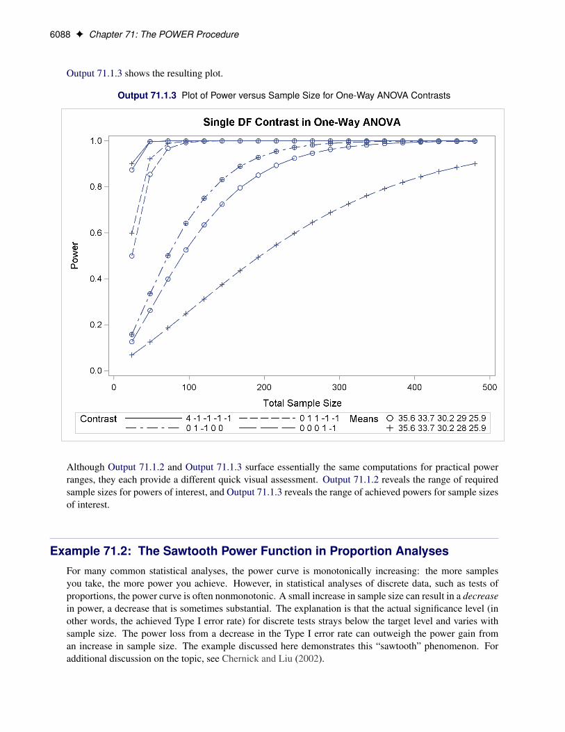
6088 F Chapter 71: The POWER Procedure
Output 71.1.3 shows the resulting plot.
Output 71.1.3 Plot of Power versus Sample Size for One-Way ANOVA Contrasts
Although Output 71.1.2 and Output 71.1.3 surface essentially the same computations for practical powerranges, they each provide a different quick visual assessment. Output 71.1.2 reveals the range of requiredsample sizes for powers of interest, and Output 71.1.3 reveals the range of achieved powers for sample sizesof interest.
Example 71.2: The Sawtooth Power Function in Proportion AnalysesFor many common statistical analyses, the power curve is monotonically increasing: the more samplesyou take, the more power you achieve. However, in statistical analyses of discrete data, such as tests ofproportions, the power curve is often nonmonotonic. A small increase in sample size can result in a decreasein power, a decrease that is sometimes substantial. The explanation is that the actual significance level (inother words, the achieved Type I error rate) for discrete tests strays below the target level and varies withsample size. The power loss from a decrease in the Type I error rate can outweigh the power gain froman increase in sample size. The example discussed here demonstrates this “sawtooth” phenomenon. Foradditional discussion on the topic, see Chernick and Liu (2002).

Example 71.2: The Sawtooth Power Function in Proportion Analyses F 6089
Suppose you have a new scheduling system for an airline, and you want to determine how many flights youmust observe to have at least an 80% chance of establishing an improvement in the proportion of late arrivalson a specific travel route. You will use a one-sided exact binomial proportion test with a null proportion of30%, the frequency of late arrivals under the previous scheduling system, and a nominal significance levelof ˛ = 0.05. Well-supported predictions estimate the new late arrival rate to be about 20%, and you willbase your sample size determination on this assumption.
The POWER procedure does not currently compute exact sample size directly for the exact binomial test.But you can get an initial estimate by computing the approximate sample size required for a z test. Usethe ONESAMPLEFREQ statement in the POWER procedure with TEST=Z and METHOD=NORMAL tocompute the approximate sample size to achieve a power of 0.8 by using the z test. The following statementsperform the analysis:
proc power;onesamplefreq test=z method=normal
sides = 1alpha = 0.05nullproportion = 0.3proportion = 0.2ntotal = .power = 0.8;
run;
The NTOTAL= option with a missing value (.) indicates sample size as the result parameter. The SIDES=1option specifies a one-sided test. The ALPHA=, NULLPROPORTION=, and POWER= options specify thesignificance level of 0.05, null value of 0.3, and target power of 0.8, respectively. The PROPORTION=option specifies your conjecture of 0.3 for the true proportion.
Output 71.2.1 Approximate Sample Size for z Test of a Proportion
The POWER ProcedureZ Test for Binomial Proportion
Fixed Scenario Elements
Method Normal approximationNumber of Sides 1Null Proportion 0.3Alpha 0.05Binomial Proportion 0.2Nominal Power 0.8Variance Estimate Null Variance
Computed N Total
Actual NPower Total
0.800 119
The results, shown in Output 71.2.1, indicate that you need to observe about N = 119 flights to have an 80%chance of rejecting the hypothesis of a late arrival proportion of 30% or higher, if the true proportion is 20%,

6090 F Chapter 71: The POWER Procedure
by using the z test. A similar analysis (Output 71.2.2) reveals an approximate sample size of N = 129 forthe z test with continuity correction, which is performed by using TEST=ADJZ:
proc power;onesamplefreq test=adjz method=normal
sides = 1alpha = 0.05nullproportion = 0.3proportion = 0.2ntotal = .power = 0.8;
run;
Output 71.2.2 Approximate Sample Size for z Test with Continuity Correction
The POWER ProcedureZ Test for Binomial Proportion with Continuity Adjustment
Fixed Scenario Elements
Method Normal approximationNumber of Sides 1Null Proportion 0.3Alpha 0.05Binomial Proportion 0.2Nominal Power 0.8Variance Estimate Null Variance
Computed N Total
Actual NPower Total
0.801 129
Based on the approximate sample size results, you decide to explore the power of the exact binomial test forsample sizes between 110 and 140. The following statements produce the plot:
ods listing style=htmlbluecml;ods graphics on;
proc power plotonly;onesamplefreq test=exact
sides = 1alpha = 0.05nullproportion = 0.3proportion = 0.2ntotal = 119power = .;
plot x=n min=110 max=140 step=1yopts=(ref=.8) xopts=(ref=119 129);
run;

Example 71.2: The Sawtooth Power Function in Proportion Analyses F 6091
The ODS LISTING STYLE=HTMLBLUECML statement specifies the HTMLBLUECML style, which issuitable for use with PROC POWER because it allows both marker symbols and line styles to vary. See thesection “ODS Styles Suitable for Use with PROC POWER” on page 6082 for more information.
The TEST=EXACT option in the ONESAMPLEFREQ statement specifies the exact binomial test, and themissing value (.) for the POWER= option indicates power as the result parameter. The PLOTONLY optionin the PROC POWER statement disables nongraphical output. The PLOT statement with X=N requests aplot with sample size on the X axis. The MIN= and MAX= options in the PLOT statement specify thesample size range. The YOPTS=(REF=) and XOPTS=(REF=) options add reference lines to highlight theapproximate sample size results. The STEP=1 option produces a point at each integer sample size. Thesample size value specified with the NTOTAL= option in the ONESAMPLEFREQ statement is overriddenby the MIN= and MAX= options in the PLOT statement. Output 71.2.3 shows the resulting plot.
Output 71.2.3 Plot of Power versus Sample Size for Exact Binomial Test
Note the sawtooth pattern in Output 71.2.3. Although the power surpasses the target level of 0.8 at N= 119, it decreases to 0.79 with N = 120 and further to 0.76 with N = 122 before rising again to 0.81with N = 123. Not until N = 130 does the power stay above the 0.8 target. Thus, a more conservativesample size recommendation of 130 might be appropriate, depending on the precise goals of the sample sizedetermination.
In addition to considering alternative sample sizes, you might also want to assess the sensitivity of thepower to inaccuracies in assumptions about the true proportion. The following statements produce a plotincluding true proportion values of 0.18 and 0.22. They are identical to the previous statements except for

6092 F Chapter 71: The POWER Procedure
the additional true proportion values specified with the PROPORTION= option in the ONESAMPLEFREQstatement.
proc power plotonly;onesamplefreq test=exact
sides = 1alpha = 0.05nullproportion = 0.3proportion = 0.18 0.2 0.22ntotal = 119power = .;
plot x=n min=110 max=140 step=1yopts=(ref=.8) xopts=(ref=119 129);
run;
Output 71.2.4 shows the resulting plot.
Output 71.2.4 Plot for Assessing Sensitivity to True Proportion Value
Example 71.2: The Sawtooth Power Function in Proportion Analyses F 6093
The plot reveals a dramatic sensitivity to the true proportion value. For N=119, the power is about 0.92 if thetrue proportion is 0.18, and as low as 0.62 if the proportion is 0.22. Note also that the power jumps occur atthe same sample sizes in all three curves; the curves are only shifted and stretched vertically. This is becausespikes and valleys in power curves are invariant to the true proportion value; they are due to changes in thecritical value of the test.
A closer look at some ancillary output from the analysis sheds light on this property of the sawtooth pattern.You can add an ODS OUTPUT statement to save the plot content corresponding to Output 71.2.3 to a dataset:
proc power plotonly;ods output plotcontent=PlotData;onesamplefreq test=exact
sides = 1alpha = 0.05nullproportion = 0.3proportion = 0.2ntotal = 119power = .;
plot x=n min=110 max=140 step=1yopts=(ref=.8) xopts=(ref=119 129);
run;
The PlotData data set contains parameter values for each point in the plot. The parameters include un-derlying characteristics of the putative test. The following statements print the critical value and actualsignificance level along with sample size and power:
proc print data=PlotData;var NTotal LowerCritVal Alpha Power;
run;

6094 F Chapter 71: The POWER Procedure
Output 71.2.5 shows the plot data.
Output 71.2.5 Numerical Content of Plot
LowerObs NTotal CritVal Alpha Power
1 110 24 0.0356 0.7292 111 24 0.0313 0.7133 112 25 0.0446 0.7714 113 25 0.0395 0.7565 114 25 0.0349 0.7416 115 26 0.0490 0.7957 116 26 0.0435 0.7818 117 26 0.0386 0.7679 118 26 0.0341 0.752
10 119 27 0.0478 0.80411 120 27 0.0425 0.79012 121 27 0.0377 0.77613 122 27 0.0334 0.76214 123 28 0.0465 0.81215 124 28 0.0414 0.79916 125 28 0.0368 0.78617 126 28 0.0327 0.77218 127 29 0.0453 0.82019 128 29 0.0404 0.80720 129 29 0.0359 0.79421 130 30 0.0493 0.83822 131 30 0.0441 0.82723 132 30 0.0394 0.81524 133 30 0.0351 0.80325 134 31 0.0480 0.84526 135 31 0.0429 0.83427 136 31 0.0384 0.82328 137 31 0.0342 0.81129 138 32 0.0466 0.85130 139 32 0.0418 0.84131 140 32 0.0374 0.830
Note that whenever the critical value changes, the actual ˛ jumps up to a value close to the nominal ˛=0.05,and the power also jumps up. Then while the critical value stays constant, the actual ˛ and power slowlydecrease. The critical value is independent of the true proportion value. So you can achieve a locallymaximal power by choosing a sample size corresponding to a spike on the sawtooth curve, and this choiceis locally optimal regardless of the unknown value of the true proportion. Locally optimal sample sizes inthis case include 115, 119, 123, 127, 130, and 134.
As a point of interest, the power does not always jump sharply and decrease gradually. The shape of thesawtooth depends on the direction of the test and the location of the null proportion relative to 0.5. Forexample, if the direction of the hypothesis in this example is reversed (by switching true and null proportionvalues) so that the rejection region is in the upper tail, then the power curve exhibits sharp decreases andgradual increases. The following statements are similar to those producing the plot in Output 71.2.3 butwith values of the PROPORTION= and NULLPROPORTION= options switched:

Example 71.2: The Sawtooth Power Function in Proportion Analyses F 6095
proc power plotonly;onesamplefreq test=exact
sides = 1alpha = 0.05nullproportion = 0.2proportion = 0.3ntotal = 119power = .;
plot x=n min=110 max=140 step=1;run;
The resulting plot is shown in Output 71.2.6.
Output 71.2.6 Plot of Power versus Sample Size for Another One-sided Test
Finally, two-sided tests can lead to even more irregular power curve shapes, since changes in lower andupper critical values affect the power in different ways. The following statements produce a plot of powerversus sample size for the scenario of a two-sided test with high alpha and a true proportion close to the nullvalue:

6096 F Chapter 71: The POWER Procedure
proc power plotonly;onesamplefreq test=exact
sides = 2alpha = 0.2nullproportion = 0.1proportion = 0.09ntotal = 10power = .;
plot x=n min=2 max=100 step=1;run;
ods graphics off;
Output 71.2.7 shows the resulting plot.
Output 71.2.7 Plot of Power versus Sample Size for a Two-Sided Test
Due to the irregular shapes of power curves for proportion tests, the question “Which sample size should Iuse?” is often insufficient. A sample size solution produced directly in PROC POWER reveals the smallestpossible sample size to achieve your target power. But as the examples in this section demonstrate, it ishelpful to consult graphs for answers to questions such as the following:
Example 71.3: Simple AB/BA Crossover Designs F 6097
� Which sample size will guarantee that all higher sample sizes also achieve my target power?
� Given a candidate sample size, can I increase it slightly to achieve locally maximal power, or perhapseven decrease it and get higher power?
Example 71.3: Simple AB/BA Crossover DesignsCrossover trials are experiments in which each subject is given a sequence of different treatments. They areespecially common in clinical trials for medical studies. The reduction in variability from taking multiplemeasurements on a subject allows for more precise treatment comparisons. The simplest such design is theAB/BA crossover, in which each subject receives each of two treatments in a randomized order.
Under certain simplifying assumptions, you can test the treatment difference in an AB/BA crossover trial byusing either a paired or two-sample t test (or equivalence test, depending on the hypothesis). This examplewill demonstrate when and how you can use the PAIREDMEANS statement in PROC POWER to performpower analyses for AB/BA crossover designs.
Senn (1993, Chapter 3) discusses a study comparing the effects of two bronchodilator medications in treat-ment of asthma, by using an AB/BA crossover design. Suppose you want to plan a similar study comparingtwo new medications, “Xilodol” and “Brantium.” Half of the patients would be assigned to sequence AB,getting a dose of Xilodol in the first treatment period, a wash-out period of one week, and then a dose ofBrantium in the second treatment period. The other half would be assigned to sequence BA, following thesame schedule but with the drugs reversed. In each treatment period you would administer the drugs in themorning and then measure peak expiratory flow (PEF) at the end of the day, with higher PEF representingbetter lung function.
You conjecture that the mean and standard deviation of PEF are about �A = 330 and �A = 40 for Xilodoland �B = 310 and �B = 55 for Brantium, and that each pair of measurements on the same subject will havea correlation of about 0.3. You want to compute the power of both one-sided and two-sided tests of meandifference, with a significance level of ˛ D 0:01, for a sample size of 100 patients and also plot the powerfor a range of 50 to 200 patients. Note that the allocation ratio of patients to the two sequences is irrelevantin this analysis.
The choice of statistical test depends on which assumptions are reasonable. One possibility is a t test. Apaired or two-sample t test is valid when there is no carryover effect and no interactions between patients,treatments, and periods. See Senn (1993, Chapter 3) for more details. The choice between a paired ora two-sample test depends on what you assume about the period effect. If you assume no period effect,then a paired t test is the appropriate analysis for the design, with the first member of each pair being theXilodol measurement (regardless of which sequence the patient belongs to). Otherwise, the two-samplet test approach is called for, since this analysis adjusts for the period effect by using an extra degree offreedom.
Suppose you assume no period effect. Then you can use the PAIREDMEANS statement in PROC POWERwith the TEST=DIFF option to perform a sample size analysis for the paired t test. Indicate power as theresult parameter by specifying the POWER= option with a missing value (.). Specify the conjectured meansand standard deviations for each drug by using the PAIREDMEANS= and PAIREDSTDDEVS= optionsand the correlation by using the CORR= option. Specify both one- and two-sided tests by using the SIDES=option, the significance level by using the ALPHA= option, and the sample size (in terms of number ofpairs) by using the NPAIRS= option. Generate a plot of power versus sample size by specifying the PLOT

6098 F Chapter 71: The POWER Procedure
statement with X=N to request a plot with sample size on the X axis. (The result parameter, here power, isalways plotted on the other axis.) Use the MIN= and MAX= options in the PLOT statement to specify thesample size range (as numbers of pairs).
The following statements perform the sample size analysis:
ods listing style=htmlbluecml;ods graphics on;
proc power;pairedmeans test=diff
pairedmeans = (330 310)pairedstddevs = (40 55)corr = 0.3sides = 1 2alpha = 0.01npairs = 100power = .;
plot x=n min=50 max=200;run;
ods graphics off;
The ODS LISTING STYLE=HTMLBLUECML statement specifies the HTMLBLUECML style, which issuitable for use with PROC POWER because it allows both marker symbols and line styles to vary. See thesection “ODS Styles Suitable for Use with PROC POWER” on page 6082 for more information.
Default values for the NULLDIFF= and DIST= options specify a null mean difference of 0 and the assump-tion of normally distributed data. The output is shown in Output 71.3.1 and Output 71.3.2.
Output 71.3.1 Power for Paired t Analysis of Crossover Design
The POWER ProcedurePaired t Test for Mean Difference
Fixed Scenario Elements
Distribution NormalMethod ExactAlpha 0.01Mean 1 330Mean 2 310Standard Deviation 1 40Standard Deviation 2 55Correlation 0.3Number of Pairs 100Null Difference 0
Computed Power
Index Sides Power
1 1 0.8652 2 0.801

Example 71.3: Simple AB/BA Crossover Designs F 6099
Output 71.3.2 Plot of Power versus Sample Size for Paired t Analysis of Crossover Design
The “Computed Power” table in Output 71.3.1 shows that the power with 100 patients is about 0.8 for thetwo-sided test and 0.87 for the one-sided test with the alternative of larger Brantium mean. In Output 71.3.2,the line style identifies the number of sides of the test. The plotting symbols identify locations of actualcomputed powers; the curves are linear interpolations of these points. The plot demonstrates how muchhigher the power is in the one-sided test than in the two-sided test for the range of sample sizes.
Suppose now that instead of detecting a difference between Xilodol and Brantium, you want to establishthat they are similar—in particular, that the absolute mean PEF difference is at most 35. You might considerthis goal if, for example, one of the drugs has fewer side effects and if a difference of no more than 35is considered clinically small. Instead of a standard t test, you would conduct an equivalence test of thetreatment mean difference for the two drugs. You would test the hypothesis that the true difference is lessthan –35 or more than 35 against the alternative that the mean difference is between –35 and 35, by usingan additive model and a two one-sided tests (“TOST”) analysis.
Assuming no period effect, you can use the PAIREDMEANS statement with the TEST=EQUIV_DIFF op-tion to perform a sample size analysis for the paired equivalence test. Indicate power as the result parameterby specifying the POWER= option with a missing value (.). Use the LOWER= and UPPER= options tospecify the equivalence bounds of –35 and 35. Use the PAIREDMEANS=, PAIREDSTDDEVS=, CORR=,and ALPHA= options in the same way as in the t test at the beginning of this example to specify the remain-ing parameters.

6100 F Chapter 71: The POWER Procedure
The following statements perform the sample size analysis:
proc power;pairedmeans test=equiv_add
lower = -35upper = 35pairedmeans = (330 310)pairedstddevs = (40 55)corr = 0.3alpha = 0.01npairs = 100power = .;
run;
The default option DIST=NORMAL specifies an assumption of normally distributed data. The output isshown in Output 71.3.3.
Output 71.3.3 Power for Paired Equivalence Test for Crossover Design
The POWER ProcedureEquivalence Test for Paired Mean Difference
Fixed Scenario Elements
Distribution NormalMethod ExactLower Equivalence Bound -35Upper Equivalence Bound 35Alpha 0.01Reference Mean 330Treatment Mean 310Standard Deviation 1 40Standard Deviation 2 55Correlation 0.3Number of Pairs 100
Computed Power
Power
0.598
The power for the paired equivalence test with 100 patients is about 0.6.
Example 71.4: Noninferiority Test with Lognormal DataThe typical goal in noninferiority testing is to conclude that a new treatment or process or product is notappreciably worse than some standard. This is accomplished by convincingly rejecting a one-sided nullhypothesis that the new treatment is appreciably worse than the standard. When designing such studies,investigators must define precisely what constitutes “appreciably worse.”

Example 71.4: Noninferiority Test with Lognormal Data F 6101
You can use the POWER procedure for sample size analyses for a variety of noninferiority tests, by specify-ing custom, one-sided null hypotheses for common tests. This example illustrates the strategy (often calledBlackwelder’s scheme; Blackwelder 1982) by comparing the means of two independent lognormal samples.The logic applies to one-sample, two-sample, and paired-sample problems involving normally distributedmeasures and proportions.
Suppose you are designing a study hoping to show that a new (less expensive) manufacturing process doesnot produce appreciably more pollution than the current process. Quantifying “appreciably worse” as 10%,you seek to show that the mean pollutant level from the new process is less than 110% of that from thecurrent process. In standard hypothesis testing notation, you seek to reject
H0W�new
�current� 1:10
in favor of
HAW�new
�current< 1:10
This is described graphically in Figure 71.8. Mean ratios below 100% are better levels for the new pro-cess; a ratio of 100% indicates absolute equivalence; ratios of 100–110% are “tolerably” worse; and ratiosexceeding 110% are appreciably worse.
Figure 71.8 Hypotheses for the Pollutant Study
An appropriate test for this situation is the common two-group t test on log-transformed data. The hypothe-ses become
H0W log .�new/ � log .�current/ � log.1:10/HAW log .�new/ � log .�current/ < log.1:10/
Measurements of the pollutant level will be taken by using laboratory models of the two processes and willbe treated as independent lognormal observations with a coefficient of variation (�=�) between 0.5 and 0.6for both processes. You will end up with 300 measurements for the current process and 180 for the new one.It is important to avoid a Type I error here, so you set the Type I error rate to 0.01. Your theoretical worksuggests that the new process will actually reduce the pollutant by about 10% (to 90% of current), but youneed to compute and graph the power of the study if the new levels are actually between 70% and 120% ofcurrent levels.
Implement the sample size analysis by using the TWOSAMPLEMEANS statement in PROC POWER withthe TEST=RATIO option. Indicate power as the result parameter by specifying the POWER= option witha missing value (.). Specify a series of scenarios for the mean ratio between 0.7 and 1.2 by using theMEANRATIO= option. Use the NULLRATIO= option to specify the null mean ratio of 1.10. SpecifySIDES=L to indicate a one-sided test with the alternative hypothesis stating that the mean ratio is lowerthan the null value. Specify the significance level, scenarios for the coefficient of variation, and the group

6102 F Chapter 71: The POWER Procedure
sample sizes by using the ALPHA=, CV=, and GROUPNS= options. Generate a plot of power versus meanratio by specifying the PLOT statement with the X=EFFECT option to request a plot with mean ratio on theX axis. (The result parameter, here power, is always plotted on the other axis.) Use the STEP= option in thePLOT statement to specify an interval of 0.05 between computed points in the plot.
The following statements perform the desired analysis:
ods listing style=htmlbluecml;ods graphics on;
proc power;twosamplemeans test=ratio
meanratio = 0.7 to 1.2 by 0.1nullratio = 1.10sides = Lalpha = 0.01cv = 0.5 0.6groupns = (300 180)power = .;
plot x=effect step=0.05;run;
ods graphics off;
The ODS LISTING STYLE=HTMLBLUECML statement specifies the HTMLBLUECML style, which issuitable for use with PROC POWER because it allows both marker symbols and line styles to vary. See thesection “ODS Styles Suitable for Use with PROC POWER” on page 6082 for more information.
Note the use of SIDES=L, which forces computations for cases that need a rejection region that is oppositeto the one providing the most one-tailed power; in this case, it is the lower tail. Such cases will show powerthat is less than the prescribed Type I error rate. The default option DIST=LOGNORMAL specifies theassumption of lognormally distributed data. The default MIN= and MAX= options in the plot statementspecify an X axis range identical to the effect size range in the TWOSAMPLEMEANS statement (meanratios between 0.7 and 1.2).
Output 71.4.1 and Output 71.4.2 show the results.
Output 71.4.1 Power for Noninferiority Test of Ratio
The POWER ProcedureTwo-Sample t Test for Mean Ratio
Fixed Scenario Elements
Distribution LognormalMethod ExactNumber of Sides LNull Geometric Mean Ratio 1.1Alpha 0.01Group 1 Sample Size 300Group 2 Sample Size 180

Example 71.4: Noninferiority Test with Lognormal Data F 6103
Output 71.4.1 continued
Computed Power
GeoMean
Index Ratio CV Power
1 0.7 0.5 >.9992 0.7 0.6 >.9993 0.8 0.5 >.9994 0.8 0.6 >.9995 0.9 0.5 0.9856 0.9 0.6 0.9337 1.0 0.5 0.4248 1.0 0.6 0.3069 1.1 0.5 0.010
10 1.1 0.6 0.01011 1.2 0.5 <.00112 1.2 0.6 <.001
Output 71.4.2 Plot of Power versus Mean Ratio for Noninferiority Test

6104 F Chapter 71: The POWER Procedure
The “Computed Power” table in Output 71.4.1 shows that power exceeds 0.90 if the true mean ratio is90% or less, as surmised. But power is unacceptably low (0.31–0.42) if the processes happen to be trulyequivalent. Note that the power is identical to the alpha level (0.01) if the true mean ratio is 1.10 and below0.01 if the true mean ratio is appreciably worse (>110%). In Output 71.4.2, the line style identifies thecoefficient of variation. The plotting symbols identify locations of actual computed powers; the curves arelinear interpolations of these points.
Example 71.5: Multiple Regression and CorrelationYou are working with a team of preventive cardiologists investigating whether elevated serum homocysteinelevels are linked to atherosclerosis (plaque buildup) in coronary arteries. The planned analysis is an ordinaryleast squares regression to assess the relationship between total homocysteine level (tHcy) and a plaqueburden index (PBI), adjusting for six other variables: age, gender, plasma levels of folate, vitamin B6,vitamin B12, and a serum cholesterol index. You will regress PBI on tHcy and the six other predictors (plusthe intercept) and use a Type III F test to assess whether tHcy is a significant predictor after adjusting forthe others. You wonder whether 100 subjects will provide adequate statistical power.
This is a correlational study at a single time. Subjects will be screened so that about half will have had a heartproblem. All eight variables will be measured during one visit. Most clinicians are familiar with simplecorrelations between two variables, so you decide to pose the statistical problem in terms of estimatingand testing the partial correlation between X1 = tHcy and Y = PBI, controlling for the six other predictorvariables (RYX1jX�1). This greatly simplifies matters, especially the elicitation of the conjectured effect.
You use partial regression plots like that shown in Figure 71.9 to teach the team that the partial correlationbetween PBI and tHcy is the correlation of two sets of residuals obtained from ordinary regression models,one from regressing PBI on the six covariates and the other from regressing tHcy on the same covariates.Thus each subject has “expected” tHcy and PBI values based on the six covariates. The cardiologists believethat subjects whose tHcy is relatively higher than expected will also have a PBI that is relatively higher thanexpected. The partial correlation quantifies that adjusted association just as a standard simple correlationdoes with the unadjusted linear association between two variables.
Figure 71.9 Partial Regression Plot

Example 71.5: Multiple Regression and Correlation F 6105
Based on previously published studies of various coronary risk factors and after viewing a set of scatterplotsshowing various correlations, the team surmises that the true partial correlation is likely to be at least 0.35.
You want to compute the statistical power for a sample size of N = 100 by using ˛ = 0.05. You alsowant to plot power for sample sizes between 50 and 150. Use the MULTREG statement to compute thepower and the PLOT statement to produce the graph. Since the predictors are observed rather than fixedin advanced, and a joint multivariate normal assumption seems tenable, use MODEL=RANDOM. Thefollowing statements perform the power analysis:
ods listing style=htmlbluecml;ods graphics on;
proc power;multreg
model = randomnfullpredictors = 7ntestpredictors = 1partialcorr = 0.35ntotal = 100power = .;
plot x=n min=50 max=150;run;
ods graphics off;
The ODS LISTING STYLE=HTMLBLUECML statement specifies the HTMLBLUECML style, which issuitable for use with PROC POWER because it allows both marker symbols and line styles to vary. See thesection “ODS Styles Suitable for Use with PROC POWER” on page 6082 for more information.
The POWER=. option identifies power as the parameter to compute. The NFULLPREDICTORS= optionspecifies seven total predictors (not including the intercept), and the NTESTPREDICTORS= option indi-cates that one of those predictors is being tested. The PARTIALCORR= and NTOTAL= options specify thepartial correlation and sample size, respectively. The default value for the ALPHA= option sets the signifi-cance level to 0.05. The X=N option in the plot statement requests a plot of sample size on the X axis, andthe MIN= and MAX= options specify the sample size range.
Output 71.5.1 shows the output, and Output 71.5.2 shows the plot.
Output 71.5.1 Power Analysis for Multiple Regression
The POWER ProcedureType III F Test in Multiple Regression
Fixed Scenario Elements
Method ExactModel Random XNumber of Predictors in Full Model 7Number of Test Predictors 1Partial Correlation 0.35Total Sample Size 100Alpha 0.05

6106 F Chapter 71: The POWER Procedure
Output 71.5.1 continued
Computed Power
Power
0.939
Output 71.5.2 Plot of Power versus Sample Size for Multiple Regression
For the sample size N = 100, the study is almost balanced with respect to Type I and Type II error rates,with ˛ = 0.05 and ˇ = 1 – 0.937 = 0.063. The study thus seems well designed at this sample size.
Now suppose that in a follow-up meeting with the cardiologists, you discover that their specific intent is todemonstrate that the (partial) correlation between PBI and tHcy is greater than 0.2. You suggest changing theplanned data analysis to a one-sided Fisher’s z test with a null correlation of 0.2. The following statementsperform a power analysis for this test:

Example 71.5: Multiple Regression and Correlation F 6107
proc power;onecorr dist=fisherz
npvars = 6corr = 0.35nullcorr = 0.2sides = 1ntotal = 100power = .;
run;
The DIST=FISHERZ option in the ONECORR statement specifies Fisher’s z test. The NPARTIALVARS=option specifies that six additional variables are adjusted for in the partial correlation. The CORR= optionspecifies the conjectured correlation of 0.35, and the NULLCORR= option indicates the null value of 0.2.The SIDES= option specifies a one-sided test.
Output 71.5.3 shows the output.
Output 71.5.3 Power Analysis for Fisher’s z Test
The POWER ProcedureFisher's z Test for Pearson Correlation
Fixed Scenario Elements
Distribution Fisher's z transformation of rMethod Normal approximationNumber of Sides 1Null Correlation 0.2Number of Variables Partialled Out 6Correlation 0.35Total Sample Size 100Nominal Alpha 0.05
Computed Power
ActualAlpha Power
0.05 0.466
The power for Fisher’s z test is less than 50%, the decrease being mostly due to the smaller effect size(relative to the null value). When asked for a recommendation for a new sample size goal, you computethe required sample size to achieve a power of 0.95 (to balance Type I and Type II errors) and 0.85 (athreshold deemed to be minimally acceptable to the team). The following statements perform the samplesize determination:

6108 F Chapter 71: The POWER Procedure
proc power;onecorr dist=fisherz
npvars = 6corr = 0.35nullcorr = 0.2sides = 1ntotal = .power = 0.85 0.95;
run;
The NTOTAL=. option identifies sample size as the parameter to compute, and the POWER= option speci-fies the target powers.
Output 71.5.4 Sample Size Determination for Fisher’s z Test
The POWER ProcedureFisher's z Test for Pearson Correlation
Fixed Scenario Elements
Distribution Fisher's z transformation of rMethod Normal approximationNumber of Sides 1Null Correlation 0.2Number of Variables Partialled Out 6Correlation 0.35Nominal Alpha 0.05
Computed N Total
Nominal Actual Actual NIndex Power Alpha Power Total
1 0.85 0.05 0.850 2802 0.95 0.05 0.950 417
The results in Output 71.5.4 reveal a required sample size of 417 to achieve a power of 0.95 and a requiredsample size of 280 to achieve a power of 0.85.
Example 71.6: Comparing Two Survival CurvesYou are consulting for a clinical research group planning a trial to compare survival rates for proposed andstandard cancer treatments. The planned data analysis is a log-rank test to nonparametrically compare theoverall survival curves for the two treatments. Your goal is to determine an appropriate sample size toachieve a power of 0.8 for a two-sided test with ˛ = 0.05 by using a balanced design.
The survival curve for patients on the standard treatment is well known to be approximately exponentialwith a median survival time of five years. The research group conjectures that the new proposed treatmentwill yield a (nonexponential) survival curve similar to the dashed line in Figure 71.6.1.
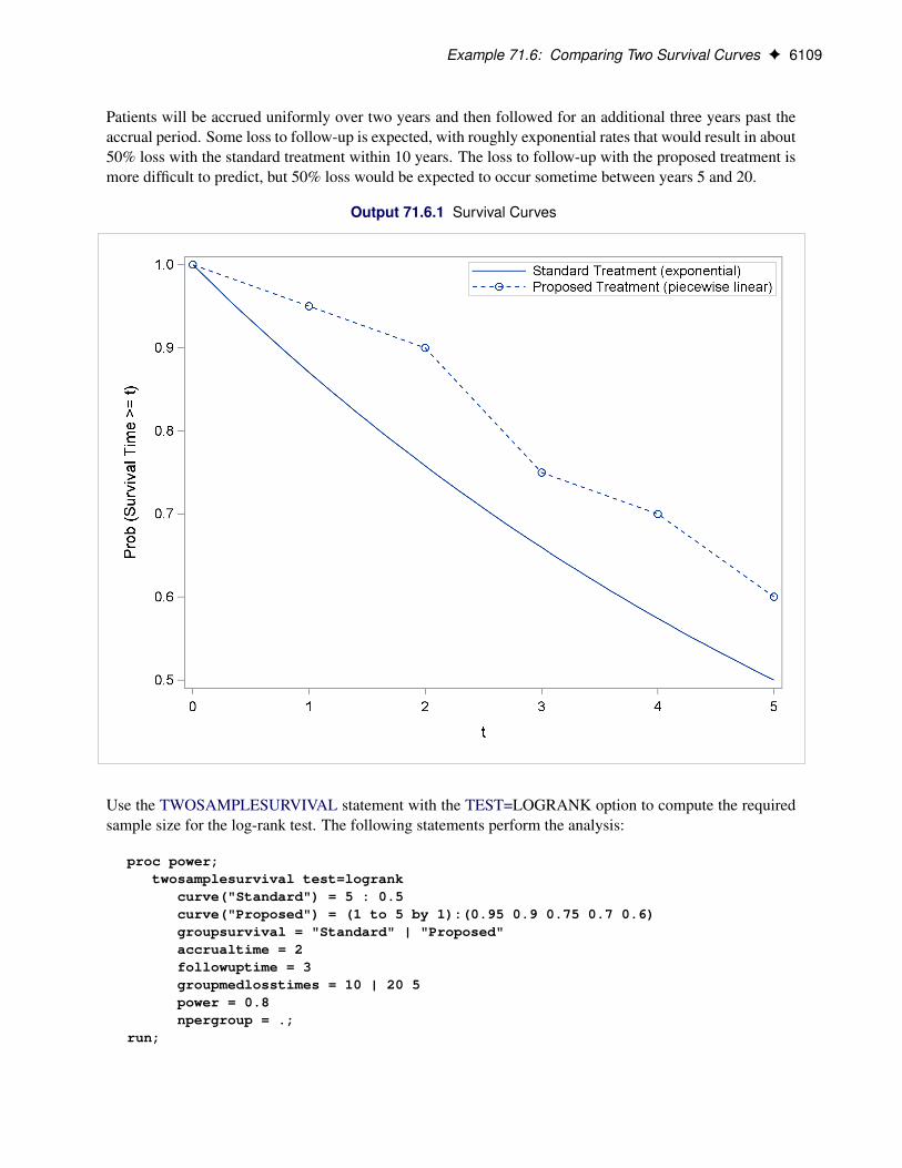
Example 71.6: Comparing Two Survival Curves F 6109
Patients will be accrued uniformly over two years and then followed for an additional three years past theaccrual period. Some loss to follow-up is expected, with roughly exponential rates that would result in about50% loss with the standard treatment within 10 years. The loss to follow-up with the proposed treatment ismore difficult to predict, but 50% loss would be expected to occur sometime between years 5 and 20.
Output 71.6.1 Survival Curves
Use the TWOSAMPLESURVIVAL statement with the TEST=LOGRANK option to compute the requiredsample size for the log-rank test. The following statements perform the analysis:
proc power;twosamplesurvival test=logrank
curve("Standard") = 5 : 0.5curve("Proposed") = (1 to 5 by 1):(0.95 0.9 0.75 0.7 0.6)groupsurvival = "Standard" | "Proposed"accrualtime = 2followuptime = 3groupmedlosstimes = 10 | 20 5power = 0.8npergroup = .;
run;

6110 F Chapter 71: The POWER Procedure
The CURVE= option defines the two survival curves. The “Standard” curve has only one point, specifyingan exponential form with a survival probability of 0.5 at year 5. The “Proposed” curve is a piecewiselinear curve defined by the five points shown in Figure 71.6.1. The GROUPSURVIVAL= option assignsthe survival curves to the two groups, and the ACCRUALTIME= and FOLLOWUPTIME= options specifythe accrual and follow-up times. The GROUPMEDLOSSTIMES= option specifies the years at which 50%loss is expected to occur. The POWER= option specifies the target power, and the NPERGROUP=. optionidentifies sample size per group as the parameter to compute. Default values for the SIDES= and ALPHA=options specify a two-sided test with ˛ = 0.05.
Output 71.6.2 shows the results.
Output 71.6.2 Sample Size Determination for Log-Rank Test
The POWER ProcedureLog-Rank Test for Two Survival Curves
Fixed Scenario Elements
Method Lakatos normal approximationAccrual Time 2Follow-up Time 3Group 1 Survival Curve StandardForm of Survival Curve 1 ExponentialGroup 2 Survival Curve ProposedForm of Survival Curve 2 Piecewise LinearGroup 1 Median Loss Time 10Nominal Power 0.8Number of Sides 2Number of Time Sub-Intervals 12Alpha 0.05
Computed N Per Group
MedianLoss Actual N Per
Index Time 2 Power Group
1 20 0.800 2282 5 0.801 234
The required sample size per group to achieve a power of 0.8 is 228 if the median loss time is 20 years forthe proposed treatment. Only six more patients are required in each group if the median loss time is as shortas five years.
Example 71.7: Confidence Interval PrecisionAn investment firm has hired you to help plan a study to estimate the success of a new investment strategycalled “IntuiVest.” The study involves complex simulations of market conditions over time, and it tracksthe balance of a hypothetical brokerage account starting with $50,000. Each simulation is very expensivein terms of computing time. You are asked to determine an appropriate number of simulations to estimate

Example 71.7: Confidence Interval Precision F 6111
the average change in the account balance at the end of three years. The goal is to have a 95% chance ofobtaining a 90% confidence interval whose half-width is at most $1,000. That is, the firm wants to havea 95% chance of being able to correctly claim at the end of the study that “Our research shows with 90%confidence that IntuiVest yields a profit of $X +/– $1,000 at the end of three years on an initial investmentof $50,000 (under simulated market conditions).”
The probability of achieving the desired precision (that is, a small interval width) can be calculated eitherunconditionally or conditionally given that the true mean is captured by the interval. You decide to use theconditional form, considering two of its advantages:
� The conditional probability is usually lower than the unconditional probability for the same samplesize, meaning that the conditional form is generally conservative.
� The overall probability of achieving the desired precision and capturing the true mean is easily com-puted as the product of the half-width probability and the confidence level. In this case, the overallprobability is 0:95 � 0:9 D 0:855.
Based on some initial simulations, you expect a standard deviation between $25,000 and $45,000 for theending account balance. You will consider both of these values in the sample size analysis.
As mentioned in the section “Overview of Power Concepts” on page 6018, an analysis of confidence intervalprecision is analogous to a traditional power analysis, with “CI Half-Width” taking the place of effect sizeand “Prob(Width)” taking the place of power. In this example, the target CI Half-Width is 1000, and thedesired Prob(Width) is 0.95.
In addition to computing sample sizes for a half-width of $1,000, you are asked to plot the required numberof simulations for a range of half-widths between $500 and $2,000. Use the ONESAMPLEMEANS state-ment with the CI=T option to implement the sample size determination. The following statements performthe analysis:
ods listing style=htmlbluecml;ods graphics on;
proc power;onesamplemeans ci=t
alpha = 0.1halfwidth = 1000stddev = 25000 45000probwidth = 0.95ntotal = .;
plot x=effect min=500 max=2000;run;
ods graphics off;
The ODS LISTING STYLE=HTMLBLUECML statement specifies the HTMLBLUECML style, which issuitable for use with PROC POWER because it allows both marker symbols and line styles to vary. See thesection “ODS Styles Suitable for Use with PROC POWER” on page 6082 for more information.
The NTOTAL=. option identifies sample size as the parameter to compute. The ALPHA=0.1 option spec-ifies a confidence level of 1 � ˛ = 0.9. The HALFWIDTH= option specifies the target half-width, and theSTDDEV= option specifies the conjectured standard deviation values. The PROBWIDTH= option specifies

6112 F Chapter 71: The POWER Procedure
the desired probability of achieving the target precision. The default value PROBTYPE=CONDITIONALspecifies that this probability is conditional on the true mean being captured by the interval. The default ofSIDES=2 indicates a two-sided interval.
Output 71.7.1 shows the output, and Output 71.7.2 shows the plot.
Output 71.7.1 Sample Size Determination for Confidence Interval Precision
The POWER ProcedureConfidence Interval for Mean
Fixed Scenario Elements
Distribution NormalMethod ExactAlpha 0.1CI Half-Width 1000Nominal Prob(Width) 0.95Number of Sides 2Prob Type Conditional
Computed N Total
ActualStd Prob N
Index Dev (Width) Total
1 25000 0.951 17882 45000 0.950 5652

Example 71.7: Confidence Interval Precision F 6113
Output 71.7.2 Plot of Sample Size versus Confidence Interval Half-Width
The number of simulations required in order to have a 95% chance of obtaining a half-width of at most1000 is between 1788 and 5652, depending on the standard deviation. The plot reveals that more than20,000 simulations would be required for a half-width of 500, assuming the higher standard deviation.
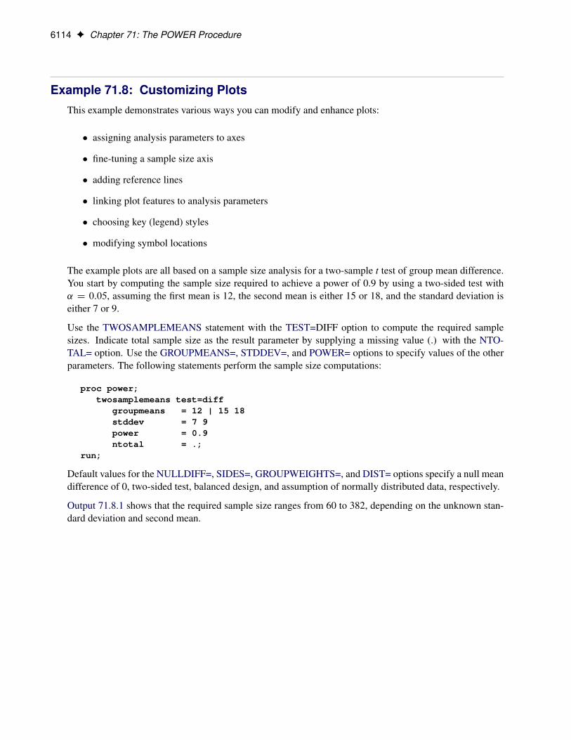
6114 F Chapter 71: The POWER Procedure
Example 71.8: Customizing PlotsThis example demonstrates various ways you can modify and enhance plots:
� assigning analysis parameters to axes
� fine-tuning a sample size axis
� adding reference lines
� linking plot features to analysis parameters
� choosing key (legend) styles
� modifying symbol locations
The example plots are all based on a sample size analysis for a two-sample t test of group mean difference.You start by computing the sample size required to achieve a power of 0.9 by using a two-sided test with˛ D 0:05, assuming the first mean is 12, the second mean is either 15 or 18, and the standard deviation iseither 7 or 9.
Use the TWOSAMPLEMEANS statement with the TEST=DIFF option to compute the required samplesizes. Indicate total sample size as the result parameter by supplying a missing value (.) with the NTO-TAL= option. Use the GROUPMEANS=, STDDEV=, and POWER= options to specify values of the otherparameters. The following statements perform the sample size computations:
proc power;twosamplemeans test=diff
groupmeans = 12 | 15 18stddev = 7 9power = 0.9ntotal = .;
run;
Default values for the NULLDIFF=, SIDES=, GROUPWEIGHTS=, and DIST= options specify a null meandifference of 0, two-sided test, balanced design, and assumption of normally distributed data, respectively.
Output 71.8.1 shows that the required sample size ranges from 60 to 382, depending on the unknown stan-dard deviation and second mean.

Example 71.8: Customizing Plots F 6115
Output 71.8.1 Computed Sample Sizes
The POWER ProcedureTwo-Sample t Test for Mean Difference
Fixed Scenario Elements
Distribution NormalMethod ExactGroup 1 Mean 12Nominal Power 0.9Number of Sides 2Null Difference 0Alpha 0.05Group 1 Weight 1Group 2 Weight 1
Computed N Total
Std Actual NIndex Mean2 Dev Power Total
1 15 7 0.902 2322 15 9 0.901 3823 18 7 0.904 604 18 9 0.904 98
Assigning Analysis Parameters to Axes
Use the PLOT statement to produce plots for all power and sample size analyses in PROC POWER. Forthe sample size analysis described at the beginning of this example, suppose you want to plot the requiredsample size on the Y axis against a range of powers between 0.5 and 0.95 on the X axis. The X= and Y=options specify which parameter to plot against the result and which axis to assign to this parameter. Youcan use either the X= or the Y= option, but not both. Use the X=POWER option in the PLOT statement torequest a plot with power on the X axis. The result parameter, here total sample size, is always plotted onthe other axis. Use the MIN= and MAX= options to specify the range of the axis indicated with either theX= or the Y= option. Here, specify MIN=0.5 and MAX=0.95 to specify the power range. The followingstatements produce the plot:
ods listing style=htmlbluecml;ods graphics on;
proc power plotonly;twosamplemeans test=diff
groupmeans = 12 | 15 18stddev = 7 9power = 0.9ntotal = .;
plot x=power min=0.5 max=0.95;run;

6116 F Chapter 71: The POWER Procedure
The ODS LISTING STYLE=HTMLBLUECML statement specifies the HTMLBLUECML style, which issuitable for use with PROC POWER because it allows both marker symbols and line styles to vary. See thesection “ODS Styles Suitable for Use with PROC POWER” on page 6082 for more information.
Note that the value (0.9) of the POWER= option in the TWOSAMPLEMEANS statement is only a place-holder when the PLOTONLY option is used and both the MIN= and MAX= options are used, because thevalues of the MIN= and MAX= options override the value of 0.9. But the POWER= option itself is stillrequired in the TWOSAMPLEMEANS statement, to provide a complete specification of the sample sizeanalysis.
The resulting plot is shown in Output 71.8.2.
Output 71.8.2 Plot of Sample Size versus Power
The line style identifies the group means scenario, and the plotting symbol identifies the standard deviationscenario. The locations of plotting symbols indicate computed sample sizes; the curves are linear interpo-lations of these points. By default, each curve consists of approximately 20 computed points (sometimesslightly more or less, depending on the analysis).
If you would rather plot power on the Y axis versus sample size on the X axis, you have two generalstrategies to choose from. One strategy is to use the Y= option instead of the X= option in the PLOTstatement:

Example 71.8: Customizing Plots F 6117
plot y=power min=0.5 max=0.95;
Output 71.8.3 Plot of Power versus Sample Size using First Strategy
Note that the resulting plot (Output 71.8.3) is essentially a mirror image of Output 71.8.2. The axis rangesare set such that each curve in Output 71.8.3 contains similar values of Y instead of X. Each plotted pointrepresents the computed value of the X axis at the input value of the Y axis.
A second strategy for plotting power versus sample size (when originally solving for sample size) is toinvert the analysis and base the plot on computed power for a given range of sample sizes. This strategyworks well for monotonic power curves (as is the case for the t test and most other continuous analyses). Itis advantageous in the sense of preserving the traditional role of the Y axis as the computed parameter. Acommon way to implement this strategy is as follows:
� Determine the range of sample sizes sufficient to cover at the desired power range for all curves(where each “curve” represents a scenario for standard deviation and second group mean).
� Use this range for the X axis of a plot.
To determine the required sample sizes for target powers of 0.5 and 0.95, change the values in the POWER=option as follows to reflect this range:
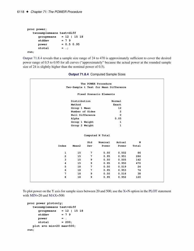
6118 F Chapter 71: The POWER Procedure
proc power;twosamplemeans test=diff
groupmeans = 12 | 15 18stddev = 7 9power = 0.5 0.95ntotal = .;
run;
Output 71.8.4 reveals that a sample size range of 24 to 470 is approximately sufficient to cover the desiredpower range of 0.5 to 0.95 for all curves (“approximately” because the actual power at the rounded samplesize of 24 is slightly higher than the nominal power of 0.5).
Output 71.8.4 Computed Sample Sizes
The POWER ProcedureTwo-Sample t Test for Mean Difference
Fixed Scenario Elements
Distribution NormalMethod ExactGroup 1 Mean 12Number of Sides 2Null Difference 0Alpha 0.05Group 1 Weight 1Group 2 Weight 1
Computed N Total
Std Nominal Actual NIndex Mean2 Dev Power Power Total
1 15 7 0.50 0.502 862 15 7 0.95 0.951 2863 15 9 0.50 0.505 1424 15 9 0.95 0.950 4705 18 7 0.50 0.519 246 18 7 0.95 0.953 747 18 9 0.50 0.516 388 18 9 0.95 0.952 120
To plot power on the Y axis for sample sizes between 20 and 500, use the X=N option in the PLOT statementwith MIN=20 and MAX=500:
proc power plotonly;twosamplemeans test=diff
groupmeans = 12 | 15 18stddev = 7 9power = .ntotal = 200;
plot x=n min=20 max=500;run;

Example 71.8: Customizing Plots F 6119
Each curve in the resulting plot in Output 71.8.5 covers at least a power range of 0.5 to 0.95.
Output 71.8.5 Plot of Power versus Sample Size Using Second Strategy
Finally, suppose you want to produce a plot of sample size versus effect size for a power of 0.9. In this case,the “effect size” is defined to be the mean difference. You need to reparameterize the analysis by using theMEANDIFF= option instead of the GROUPMEANS= option to produce a plot, since each plot axis mustbe represented by a scalar parameter. Use the X=EFFECT option in the PLOT statement to assign the meandifference to the X axis. The following statements produce a plot of required sample size to detect meandifferences between 3 and 6:
proc power plotonly;twosamplemeans test=diff
meandiff = 3 6stddev = 7 9power = 0.9ntotal = .;
plot x=effect min=3 max=6;run;
The resulting plot Output 71.8.6 shows how the required sample size decreases with increasing mean differ-ence.
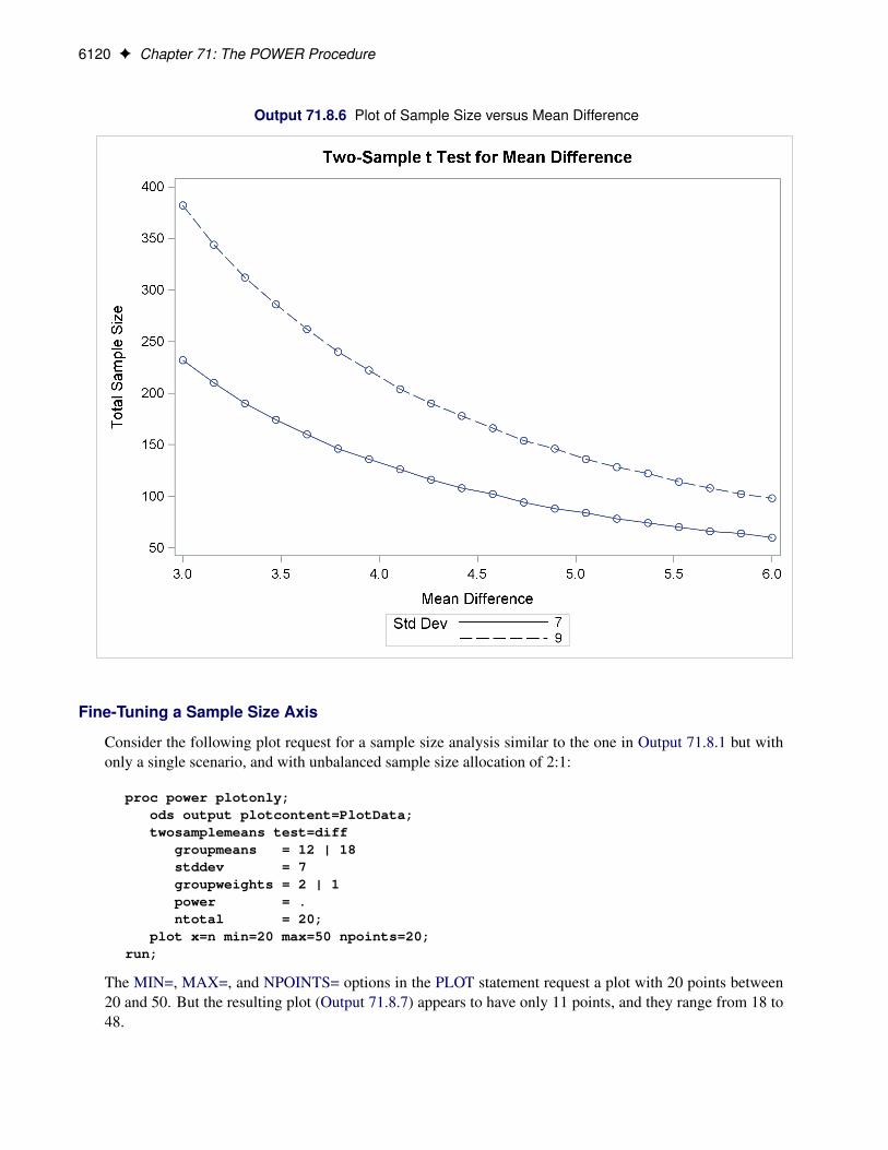
6120 F Chapter 71: The POWER Procedure
Output 71.8.6 Plot of Sample Size versus Mean Difference
Fine-Tuning a Sample Size Axis
Consider the following plot request for a sample size analysis similar to the one in Output 71.8.1 but withonly a single scenario, and with unbalanced sample size allocation of 2:1:
proc power plotonly;ods output plotcontent=PlotData;twosamplemeans test=diff
groupmeans = 12 | 18stddev = 7groupweights = 2 | 1power = .ntotal = 20;
plot x=n min=20 max=50 npoints=20;run;
The MIN=, MAX=, and NPOINTS= options in the PLOT statement request a plot with 20 points between20 and 50. But the resulting plot (Output 71.8.7) appears to have only 11 points, and they range from 18 to48.

Example 71.8: Customizing Plots F 6121
Output 71.8.7 Plot with Overlapping Points
The reason that this plot has fewer points than usual is due to the rounding of sample sizes. If you do notuse the NFRACTIONAL option in the analysis statement (here, the TWOSAMPLEMEANS statement),then the set of sample size points determined by the MIN=, MAX=, NPOINTS=, and STEP= options in thePLOT statement can be rounded to satisfy the allocation weights. In this case, they are rounded down to thenearest multiples of 3 (the sum of the weights), and many of the points overlap. To see the overlap, you canprint the NominalNTotal (unadjusted) and NTotal (rounded) variables in the PlotContent ODS object (heresaved to a data set called PlotData):
proc print data=PlotData;var NominalNTotal NTotal;
run;

6122 F Chapter 71: The POWER Procedure
The output is shown in Output 71.8.8.
Output 71.8.8 Sample Sizes
NominalObs NTotal NTotal
1 18.0 182 19.6 183 21.2 214 22.7 215 24.3 246 25.9 247 27.5 278 29.1 279 30.6 30
10 32.2 3011 33.8 3312 35.4 3313 36.9 3614 38.5 3615 40.1 3916 41.7 3917 43.3 4218 44.8 4219 46.4 4520 48.0 48
Besides overlapping of sample size points, another peculiarity that might occur without the NFRAC-TIONAL option is unequal spacing—for example, in the plot in Output 71.8.9, created with the followingstatements:
proc power plotonly;twosamplemeans test=diff
groupmeans = 12 | 18stddev = 7groupweights = 2 | 1power = .ntotal = 20;
plot x=n min=20 max=50 npoints=5;run;
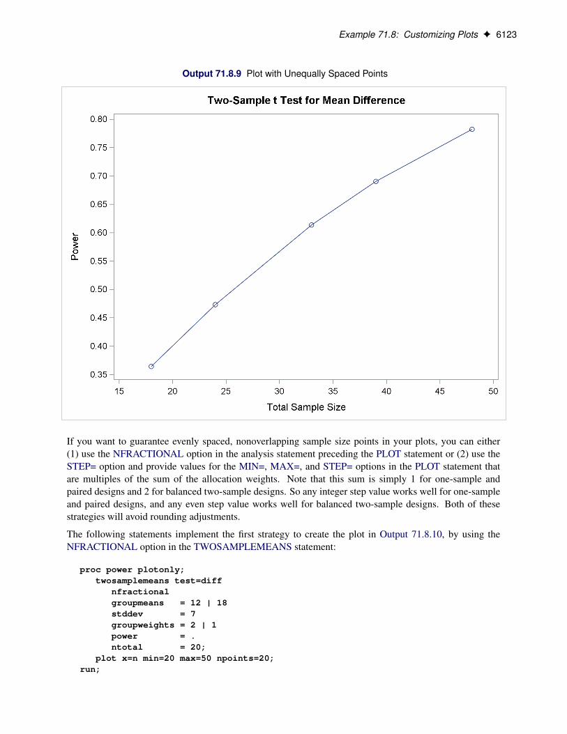
Example 71.8: Customizing Plots F 6123
Output 71.8.9 Plot with Unequally Spaced Points
If you want to guarantee evenly spaced, nonoverlapping sample size points in your plots, you can either(1) use the NFRACTIONAL option in the analysis statement preceding the PLOT statement or (2) use theSTEP= option and provide values for the MIN=, MAX=, and STEP= options in the PLOT statement thatare multiples of the sum of the allocation weights. Note that this sum is simply 1 for one-sample andpaired designs and 2 for balanced two-sample designs. So any integer step value works well for one-sampleand paired designs, and any even step value works well for balanced two-sample designs. Both of thesestrategies will avoid rounding adjustments.
The following statements implement the first strategy to create the plot in Output 71.8.10, by using theNFRACTIONAL option in the TWOSAMPLEMEANS statement:
proc power plotonly;twosamplemeans test=diff
nfractionalgroupmeans = 12 | 18stddev = 7groupweights = 2 | 1power = .ntotal = 20;
plot x=n min=20 max=50 npoints=20;run;

6124 F Chapter 71: The POWER Procedure
Output 71.8.10 Plot with Fractional Sample Sizes
To implement the second strategy, use multiples of 3 for the STEP=, MIN=, and MAX= options in thePLOT statement (because the sum of the allocation weights is 2 + 1 = 3). The following statements useSTEP=3, MIN=18, and MAX=48 to create a plot that looks identical to the plot in Output 71.8.7 but suffersno overlapping of points:
proc power plotonly;twosamplemeans test=diff
groupmeans = 12 | 18stddev = 7groupweights = 2 | 1power = .ntotal = 20;
plot x=n min=18 max=48 step=3;run;

Example 71.8: Customizing Plots F 6125
Adding Reference Lines
Suppose you want to add reference lines to highlight power=0.8 and power=0.9 on the plot in Output 71.8.5.You can add simple reference lines by using the YOPTS= option and REF= suboption in the PLOT statementto produce Output 71.8.11, with the following statements:
proc power plotonly;twosamplemeans test=diff
groupmeans = 12 | 15 18stddev = 7 9power = .ntotal = 100;
plot x=n min=20 max=500yopts=(ref=0.8 0.9);
run;
Output 71.8.11 Plot with Simple Reference Lines on Y Axis
Or you can specify CROSSREF=YES to add reference lines that intersect each curve and cross over to theother axis:
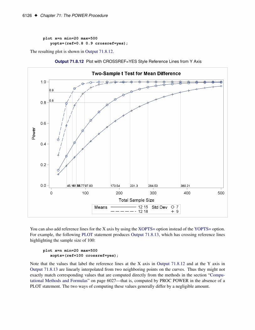
6126 F Chapter 71: The POWER Procedure
plot x=n min=20 max=500yopts=(ref=0.8 0.9 crossref=yes);
The resulting plot is shown in Output 71.8.12.
Output 71.8.12 Plot with CROSSREF=YES Style Reference Lines from Y Axis
You can also add reference lines for the X axis by using the XOPTS= option instead of the YOPTS= option.For example, the following PLOT statement produces Output 71.8.13, which has crossing reference lineshighlighting the sample size of 100:
plot x=n min=20 max=500xopts=(ref=100 crossref=yes);
Note that the values that label the reference lines at the X axis in Output 71.8.12 and at the Y axis inOutput 71.8.13 are linearly interpolated from two neighboring points on the curves. Thus they might notexactly match corresponding values that are computed directly from the methods in the section “Compu-tational Methods and Formulas” on page 6027—that is, computed by PROC POWER in the absence of aPLOT statement. The two ways of computing these values generally differ by a negligible amount.
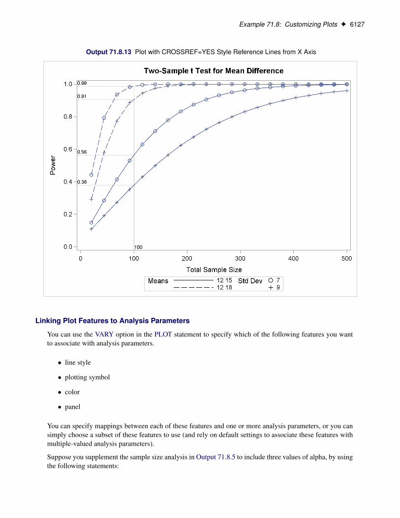
Example 71.8: Customizing Plots F 6127
Output 71.8.13 Plot with CROSSREF=YES Style Reference Lines from X Axis
Linking Plot Features to Analysis Parameters
You can use the VARY option in the PLOT statement to specify which of the following features you wantto associate with analysis parameters.
� line style
� plotting symbol
� color
� panel
You can specify mappings between each of these features and one or more analysis parameters, or you cansimply choose a subset of these features to use (and rely on default settings to associate these features withmultiple-valued analysis parameters).
Suppose you supplement the sample size analysis in Output 71.8.5 to include three values of alpha, by usingthe following statements:

6128 F Chapter 71: The POWER Procedure
proc power plotonly;twosamplemeans test=diff
groupmeans = 12 | 15 18stddev = 7 9alpha = 0.01 0.025 0.1power = .ntotal = 100;
plot x=n min=20 max=500;run;
The defaults for the VARY option in the PLOT statement specify line style varying by the ALPHA= parame-ter, plotting symbol varying by the GROUPMEANS= parameter, panel varying by the STDDEV= parameter,and color remaining constant. The resulting plot, consisting of two panels, is shown in Output 71.8.14.
Output 71.8.14 Plot with Default VARY Settings

Example 71.8: Customizing Plots F 6129
Output 71.8.14 continued
Suppose you want to produce a plot with only one panel that varies color in addition to line style andplotting symbol. Include the LINESTYLE, SYMBOL, and COLOR keywords in the VARY option in thePLOT statement, as follows, to produce the plot in Output 71.8.15:
plot x=n min=20 max=500vary (linestyle, symbol, color);

6130 F Chapter 71: The POWER Procedure
Output 71.8.15 Plot with Varying Color Instead of Panel
Finally, suppose you want to specify which features are used and which analysis parameters they are linkedto. The following PLOT statement produces a two-panel plot (shown in Output 71.8.16) in which line stylevaries by standard deviation, plotting symbol varies by both alpha and sides, and panel varies by means:
plot x=n min=20 max=500vary (linestyle by stddev,
symbol by alpha sides,panel by groupmeans);

Example 71.8: Customizing Plots F 6131
Output 71.8.16 Plot with Features Explicitly Linked to Parameters

6132 F Chapter 71: The POWER Procedure
Output 71.8.16 continued
Choosing Key (Legend) Styles
The default style for the key (or “legend”) is one that displays the association between levels of features andlevels of analysis parameters, located below the X axis. For example, Output 71.8.5 demonstrates this styleof key.
You can reproduce Output 71.8.5 with the same key but a different location, inside the plotting region, byusing the POS=INSET option within the KEY=BYFEATURE option in the PLOT statement. The followingstatements product the plot in Output 71.8.17:
proc power plotonly;twosamplemeans test=diff
groupmeans = 12 | 15 18stddev = 7 9power = .ntotal = 200;
plot x=n min=20 max=500key = byfeature(pos=inset);
run;

Example 71.8: Customizing Plots F 6133
Output 71.8.17 Plot with a By-Feature Key inside the Plotting Region
Alternatively, you can specify a key that identifies each individual curve separately by number by using theKEY=BYCURVE option in the PLOT statement:
plot x=n min=20 max=500key = bycurve;
The resulting plot is shown in Output 71.8.18.

6134 F Chapter 71: The POWER Procedure
Output 71.8.18 Plot with a Numbered By-Curve Key
Use the NUMBERS=OFF option within the KEY=BYCURVE option to specify a nonnumbered key thatidentifies curves with samples of line styles, symbols, and colors:
plot x=n min=20 max=500key = bycurve(numbers=off pos=inset);
The POS=INSET suboption places the key within the plotting region. The resulting plot is shown in Out-put 71.8.19.
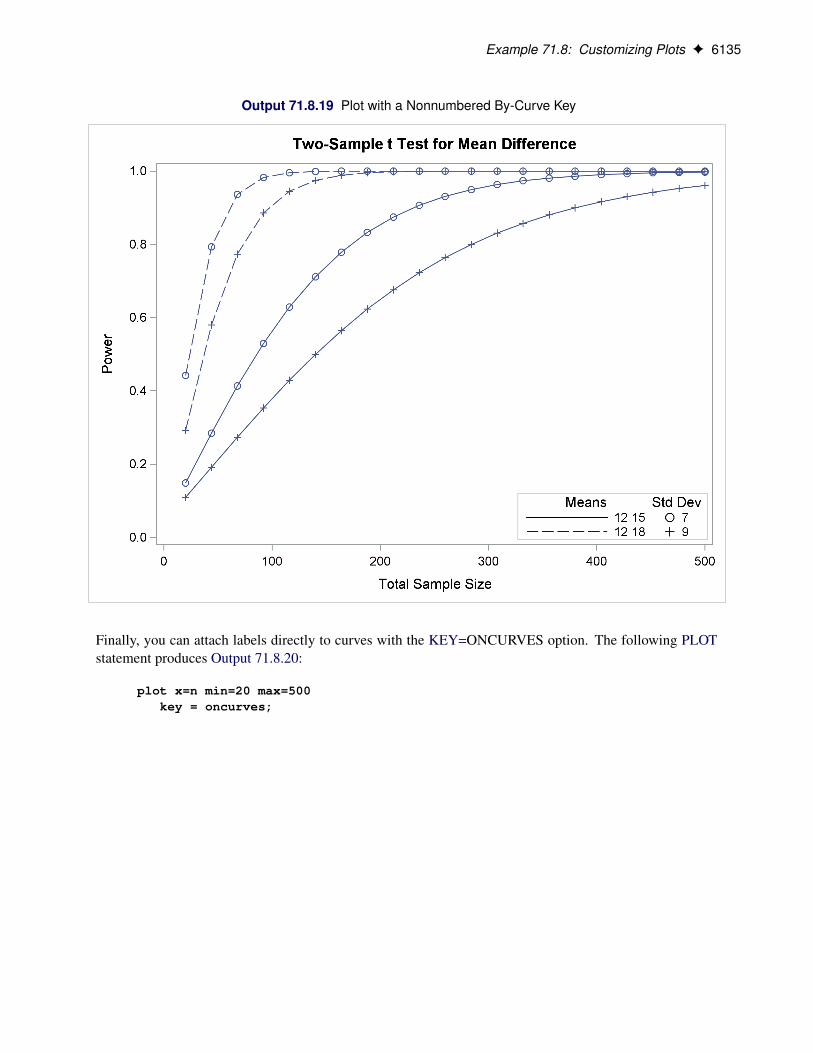
Example 71.8: Customizing Plots F 6135
Output 71.8.19 Plot with a Nonnumbered By-Curve Key
Finally, you can attach labels directly to curves with the KEY=ONCURVES option. The following PLOTstatement produces Output 71.8.20:
plot x=n min=20 max=500key = oncurves;

6136 F Chapter 71: The POWER Procedure
Output 71.8.20 Plot with Directly Labeled Curves
Modifying Symbol Locations
The default locations for plotting symbols are the points computed directly from the power and samplesize algorithms. For example, Output 71.8.5 shows plotting symbols corresponding to computed points.The curves connecting these points are interpolated (as indicated by the INTERPOL= option in the PLOTstatement).
You can modify the locations of plotting symbols by using the MARKERS= option in the PLOT statement.The MARKERS=ANALYSIS option places plotting symbols at locations corresponding to the input spec-ified in the analysis statement preceding the PLOT statement. You might prefer this as an alternative tousing reference lines to highlight specific points. For example, you can reproduce Output 71.8.5, but withthe plotting symbols located at the sample sizes shown in Output 71.8.1, by using the following statements:
proc power plotonly;twosamplemeans test=diff
groupmeans = 12 | 15 18stddev = 7 9power = .ntotal = 232 382 60 98;

Example 71.8: Customizing Plots F 6137
plot x=n min=20 max=500markers=analysis;
run;
The analysis statement here is the TWOSAMPLEMEANS statement. The MARKERS=ANALYSIS optionin the PLOT statement causes the plotting symbols to occur at sample sizes specified by the NTOTAL=option in the TWOSAMPLEMEANS statement: 232, 382, 60, and 98. The resulting plot is shown inOutput 71.8.21.
Output 71.8.21 Plot with MARKERS=ANALYSIS
You can also use the MARKERS=NICE option to align symbols with the tick marks on one of the axes (theX axis when the X= option is used, or the Y axis when the Y= option is used):
plot x=n min=20 max=500markers=nice;
The plot created by this PLOT statement is shown in Output 71.8.22.
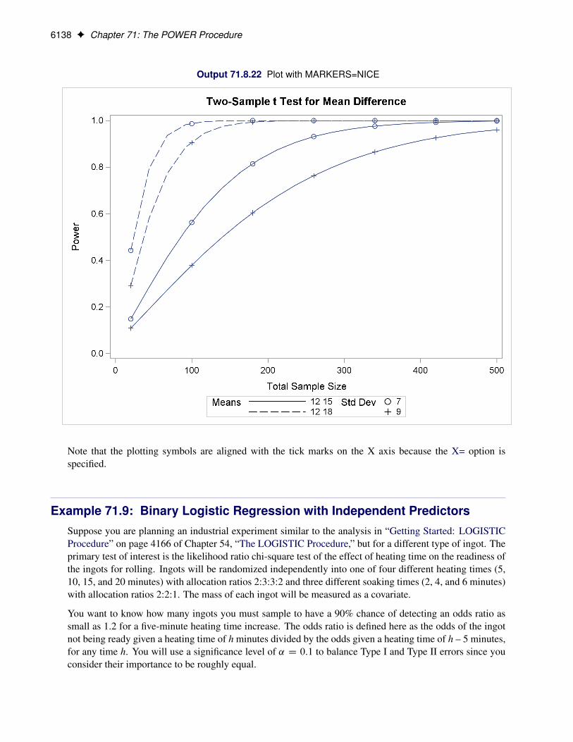
6138 F Chapter 71: The POWER Procedure
Output 71.8.22 Plot with MARKERS=NICE
Note that the plotting symbols are aligned with the tick marks on the X axis because the X= option isspecified.
Example 71.9: Binary Logistic Regression with Independent PredictorsSuppose you are planning an industrial experiment similar to the analysis in “Getting Started: LOGISTICProcedure” on page 4166 of Chapter 54, “The LOGISTIC Procedure,” but for a different type of ingot. Theprimary test of interest is the likelihood ratio chi-square test of the effect of heating time on the readiness ofthe ingots for rolling. Ingots will be randomized independently into one of four different heating times (5,10, 15, and 20 minutes) with allocation ratios 2:3:3:2 and three different soaking times (2, 4, and 6 minutes)with allocation ratios 2:2:1. The mass of each ingot will be measured as a covariate.
You want to know how many ingots you must sample to have a 90% chance of detecting an odds ratio assmall as 1.2 for a five-minute heating time increase. The odds ratio is defined here as the odds of the ingotnot being ready given a heating time of h minutes divided by the odds given a heating time of h – 5 minutes,for any time h. You will use a significance level of ˛ D 0:1 to balance Type I and Type II errors since youconsider their importance to be roughly equal.

Example 71.9: Binary Logistic Regression with Independent Predictors F 6139
The distributions of heating time and soaking time are determined by the design, but you must conjecturethe distribution of ingot mass. Suppose you expect its distribution to be approximately normal with mean 4kg and standard deviation between 1 kg and 2 kg.
You are powering the study for an odds ratio of 1.2 for the heating time, but you must also conjecture oddsratios for soaking time and mass. You suspect that the odds ratio for a unit increase in soaking time is about1.4, and the odds ratio for a unit increase in mass is between 1 and 1.3.
Finally, you must provide a guess for the average probability of an ingot not being ready for rolling, averagedacross all possible design profiles. Existing data suggest that this probability lies between 0.15 and 0.25.
You decide to evaluate sample size at the two extremes of each parameter for which you conjectured a range.Use the following statements to perform the sample size determination:
proc power;logistic
vardist("Heat") = ordinal((5 10 15 20) : (0.2 0.3 0.3 0.2))vardist("Soak") = ordinal((2 4 6) : (0.4 0.4 0.2))vardist("Mass1") = normal(4, 1)vardist("Mass2") = normal(4, 2)testpredictor = "Heat"covariates = "Soak" | "Mass1" "Mass2"responseprob = 0.15 0.25testoddsratio = 1.2units= ("Heat" = 5)covoddsratios = 1.4 | 1 1.3alpha = 0.1power = 0.9ntotal = .;
run;
The VARDIST= option is used to define the distributions of the predictor variables. The distributions of heat-ing and soaking times are defined by the experimental design, with ordinal probabilities derived from the al-location ratios. The two conjectured standard deviations for the ingot mass are represented in the Mass1 andMass2 distributions. The TESTPREDICTOR= option identifies the predictor being tested, and the COVARI-ATES= option specifies the scenarios for the remaining predictors in the model (soaking time and mass).The RESPONSEPROB= option specifies the overall response probability, and the TESTODDSRATIO= andUNITS= options indicate the odds ratio and increment for heating time. The COVODDSRATIOS= optionspecifies the scenarios for the odds ratios of soaking time and mass. The default DEFAULTUNIT=1 optionspecifies a unit change for both of these odds ratios. The ALPHA= option sets the significance level, and thePOWER= option defines the target power. Finally, the NTOTAL= option with a missing value (.) identifiesthe parameter to solve for.
Output 71.9.1 shows the results.

6140 F Chapter 71: The POWER Procedure
Output 71.9.1 Sample Sizes for Test of Heating Time in Logistic Regression
The POWER ProcedureLikelihood Ratio Chi-Square Test for One Predictor
Fixed Scenario Elements
Method Shieh-O'Brien approximationAlpha 0.1Test Predictor HeatOdds Ratio for Test Predictor 1.2Unit for Test Pred Odds Ratio 5Nominal Power 0.9
Computed N Total
TotalResponse N Actual N
Index Prob -Covariates- --Cov ORs- -Cov Units- Bins Power Total
1 0.15 Soak Mass1 1.4 1.0 1 1 120 0.900 18782 0.15 Soak Mass1 1.4 1.3 1 1 120 0.900 18723 0.15 Soak Mass2 1.4 1.0 1 1 120 0.900 18784 0.15 Soak Mass2 1.4 1.3 1 1 120 0.900 18575 0.25 Soak Mass1 1.4 1.0 1 1 120 0.900 13426 0.25 Soak Mass1 1.4 1.3 1 1 120 0.900 13487 0.25 Soak Mass2 1.4 1.0 1 1 120 0.900 13428 0.25 Soak Mass2 1.4 1.3 1 1 120 0.900 1369
The required sample size ranges from 1342 to 1878, depending on the unknown true values of the overallresponse probability, mass standard deviation, and soaking time odds ratio. The overall response probabilityclearly has the largest influence among these parameters, with a sample size increase of almost 40% goingfrom 0.25 to 0.15.
Example 71.10: Wilcoxon-Mann-Whitney TestConsider a hypothetical clinical trial to treat interstitial cystitis (IC), a painful, chronic inflammatory con-dition of the bladder with no known cause that most commonly affects women. Two treatments will becompared: lidocaine alone (“lidocaine”) versus lidocaine plus a fictitious experimental drug called Mironel(“Mir+lido”). The design is balanced, randomized, double-blind, and female-only. The primary outcome isa measure of overall improvement at week 4 of the study, measured on a seven-point Likert scale as shownin Table 71.34.

Example 71.10: Wilcoxon-Mann-Whitney Test F 6141
Table 71.34 Self-Report Improvement Scale
Compared to when I startedthis study, my condition is:
Much worse –3Worse –2Slightly worse –1The same 0Slightly better +1Better +2Much better +3
The planned data analysis is a one-sided Wilcoxon-Mann-Whitney test with ˛ D 0:05 where the alternativehypothesis represents greater improvement for “Mir+lido.”
You are asked to graphically assess the power of the planned trial for sample sizes between 100 and 250,assuming that the conditional outcome probabilities given treatment are equal to the values in Table 71.35.
Table 71.35 Conjectured Conditional Probabilities
ResponseTreatment –3 –2 –1 0 +1 +2 +3Lidocaine 0.01 0.04 0.20 0.50 0.20 0.04 0.01Mir+lido 0.01 0.03 0.15 0.35 0.30 0.10 0.06
Use the following statements to compute the power at sample sizes of 100 and 250 and generate a powercurve:
ods listing style=htmlbluecml;ods graphics on;
proc power;twosamplewilcoxon
vardist("lidocaine") = ordinal ((-3 -2 -1 0 1 2 3) :(.01 .04 .20 .50 .20 .04 .01))
vardist("Mir+lido") = ordinal ((-3 -2 -1 0 1 2 3) :(.01 .03 .15 .35 .30 .10 .06))
variables = "lidocaine" | "Mir+lido"sides = untotal = 100 250power = .;
plot step=10;run;
ods graphics off;
The ODS LISTING STYLE=HTMLBLUECML statement specifies the HTMLBLUECML style, which issuitable for use with PROC POWER because it allows both marker symbols and line styles to vary. See thesection “ODS Styles Suitable for Use with PROC POWER” on page 6082 for more information.

6142 F Chapter 71: The POWER Procedure
The VARDIST= option is used to define the distribution for each treatment, and the VARIABLES= optionspecifies the distributions to compare. The SIDES=U option corresponds to the alternative hypothesis thatthe second distribution ("Mir+lido") is more favorable. The NTOTAL= option specifies the total samplesizes of interest, and the POWER= option with a missing value (.) identifies the parameter to solve for.The default GROUPWEIGHTS= and ALPHA= options specify a balanced design and significance level˛ D 0:05.
The STEP=10 option in the PLOT statement requests a point for each sample size increment of 10. Thedefault values for the X=, MIN=, and MAX= plot options specify a sample size range of 100 to 250 (thesame as in the analysis) for the X axis.
The tabular and graphical results are shown in Output 71.10.1 and Output 71.10.2, respectively.
Output 71.10.1 Power Values for Wilcoxon-Mann-Whitney Test
The POWER ProcedureWilcoxon-Mann-Whitney Test
Fixed Scenario Elements
Method O'Brien-Castelloe approximationNumber of Sides UGroup 1 Variable lidocaineGroup 2 Variable Mir+lidoPooled Number of Bins 7Alpha 0.05Group 1 Weight 1Group 2 Weight 1NBins Per Group 1000
Computed Power
NIndex Total Power
1 100 0.6512 250 0.939
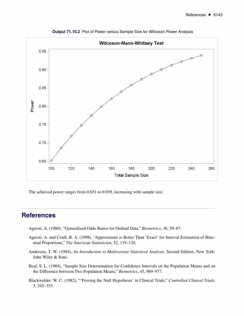
References F 6143
Output 71.10.2 Plot of Power versus Sample Size for Wilcoxon Power Analysis
The achieved power ranges from 0.651 to 0.939, increasing with sample size.
References
Agresti, A. (1980), “Generalized Odds Ratios for Ordinal Data,” Biometrics, 36, 59–67.
Agresti, A. and Coull, B. A. (1998), “Approximate is Better Than ‘Exact’ for Interval Estimation of Bino-mial Proportions,” The American Statistician, 52, 119–126.
Anderson, T. W. (1984), An Introduction to Multivariate Statistical Analysis, Second Edition, New York:John Wiley & Sons.
Beal, S. L. (1989), “Sample Size Determination for Confidence Intervals on the Population Means and onthe Difference between Two Population Means,” Biometrics, 45, 969–977.
Blackwelder, W. C. (1982), “‘Proving the Null Hypothesis’ in Clinical Trials,” Controlled Clinical Trials,3, 345–353.

6144 F Chapter 71: The POWER Procedure
Brown, L. D., Cai, T. T., and DasGupta, A. (2001), “Interval Estimation for a Binomial Proportion,” Statis-tical Science, 16, 101–133.
Cantor, A. B. (1997), Extending SAS Survival Analysis Techniques for Medical Research, Cary, NC: SASPress.
Castelloe, J. M. (2000), “Sample Size Computations and Power Analysis with the SAS System,” in Pro-ceedings of the Twenty-fifth Annual SAS Users Group International Conference, Cary, NC: SAS InstituteInc.
Castelloe, J. M. and O’Brien, R. G. (2001), “Power and Sample Size Determination for Linear Models,”in Proceedings of the Twenty-sixth Annual SAS Users Group International Conference, Cary, NC: SASInstitute Inc.
Chernick, M. R. and Liu, C. Y. (2002), “The Saw-Toothed Behavior of Power Versus Sample Size andSoftware Solutions: Single Binomial Proportion Using Exact Methods,” The American Statistician, 56,149–155.
Chow, S.-C., Shao, J., and Wang, H. (2003), Sample Size Calculations in Clinical Research, Boca Raton,FL: CRC Press.
Connor, R. J. (1987), “Sample Size for Testing Differences in Proportions for the Paired-Sample Design,”Biometrics, 43, 207–211.
Diegert, C. and Diegert, K. V. (1981), “Note on Inversion of Casagrande-Pike-Smith Approximate Sample-Size Formula for Fisher-Irwin Test on 2 � 2 Tables,” Biometrics, 37, 595.
Diletti, D., Hauschke, D., and Steinijans, V. W. (1991), “Sample Size Determination for BioequivalenceAssessment by Means of Confidence Intervals,” International Journal of Clinical Pharmacology, Therapyand Toxicology, 29, 1–8.
DiSantostefano, R. L. and Muller, K. E. (1995), “A Comparison of Power Approximations for Satterth-waite’s Test,” Communications in Statistics—Simulation and Computation, 24, 583–593.
Fisher, R. A. (1921), “On the ‘Probable Error’ of a Coefficient of Correlation Deduced from a Small Sam-ple,” Metron, 1, 3–32.
Fleiss, J. L., Tytun, A., and Ury, H. K. (1980), “A Simple Approximation for Calculating Sample Sizes forComparing Independent Proportions,” Biometrics, 36, 343–346.
Gatsonis, C. and Sampson, A. R. (1989), “Multiple Correlation: Exact Power and Sample Size Calcula-tions,” Psychological Bulletin, 106, 516–524.
Hocking, R. R. (1985), The Analysis of Linear Models, Belmont, CA: Brooks/Cole.
Hsieh, F. Y. (1989), “Sample Size Tables for Logistic Regression,” Statistics in Medicine, 8, 795–802.
Johnson, N. L. and Kotz, S. (1970), Distributions in Statistics: Continuous Univariate Distributions — 1,New York: John Wiley & Sons.
Johnson, N. L., Kotz, S., and Balakrishnan, N. (1994), Continuous Univariate Distributions, volume 1,Second Edition, New York: John Wiley & Sons.

References F 6145
Johnson, N. L., Kotz, S., and Balakrishnan, N. (1995), Continuous Univariate Distributions, volume 2,Second Edition, New York: John Wiley & Sons.
Johnson, N. L., Kotz, S., and Kemp, A. W. (1992), Univariate Discrete Distributions, Second Edition, NewYork: John Wiley & Sons.
Jones, R. M. and Miller, K. S. (1966), “On the Multivariate Lognormal Distribution,” Journal of IndustrialMathematics, 16, 63–76.
Kolassa, J. E. (1995), “A Comparison of Size and Power Calculations for the Wilcoxon Statistic for OrderedCategorical Data,” Statistics in Medicine, 14, 1577–1581.
Lachin, J. M. (1992), “Power and Sample Size Evaluation for the McNemar Test with Application toMatched Case-Control Studies,” Statistics in Medicine, 11, 1239–1251.
Lakatos, E. (1988), “Sample Sizes Based on the Log-Rank Statistic in Complex Clinical Trials,” Biometrics,44, 229–241.
Lenth, R. V. (2001), “Some Practical Guidelines for Effective Sample Size Determination,” The AmericanStatistician, 55, 187–193.
Maxwell, S. E. (2000), “Sample Size and Multiple Regression Analysis,” Psychological Methods, 5, 434–458.
Miettinen, O. S. (1968), “The Matched Pairs Design in the Case of All-or-None Responses,” Biometrics,24, 339–352.
Moser, B. K., Stevens, G. R., and Watts, C. L. (1989), “The Two-Sample T Test versus Satterthwaite’sApproximate F Test,” Communications in Statistics A—Theory and Methods, 18, 3963–3975.
Muller, K. E. and Benignus, V. A. (1992), “Increasing Scientific Power with Statistical Power,” Neurotoxi-cology and Teratology, 14, 211–219.
O’Brien, R. G. and Castelloe, J. (2007), “Sample-Size Analysis for Traditional Hypothesis Testing: Con-cepts and Issues,” in A. Dmitrienko, C. Chuang-Stein, and R. D’Agostino, eds., Pharmaceutical StatisticsUsing SAS: A Practical Guide, 237–271, Cary, NC: SAS Institute Inc.
O’Brien, R. G. and Castelloe, J. M. (2006), “Exploiting the Link between the Wilcoxon-Mann-Whitney Testand a Simple Odds Statistic,” in Proceedings of the Thirty-First Annual SAS Users Group InternationalConference, Cary, NC: SAS Institute Inc, paper 209-31.
O’Brien, R. G. and Muller, K. E. (1993), “Unified Power Analysis for t-Tests through Multivariate Hy-potheses,” in L. K. Edwards, ed., Applied Analysis of Variance in Behavioral Science, 297–344, NewYork: Marcel Dekker.
Owen, D. B. (1965), “A Special Case of a Bivariate Non-central t-Distribution,” Biometrika, 52, 437–446.
Pagano, M. and Gauvreau, K. (1993), Principles of Biostatistics, Belmont, CA: Wadsworth.
Phillips, K. F. (1990), “Power of the Two One-Sided Tests Procedure in Bioequivalence,” Journal of Phar-macokinetics and Biopharmaceutics, 18, 137–144.
Satterthwaite, F. E. (1946), “An Approximate Distribution of Estimates of Variance Components,” Biomet-rics Bulletin, 2, 110–114.

6146 F Chapter 71: The POWER Procedure
Schork, M. and Williams, G. (1980), “Number of Observations Required for the Comparison of Two Cor-related Proportions,” Communications in Statistics—Simulation and Computation, 9, 349–357.
Schuirmann, D. J. (1987), “A Comparison of the Two One-Sided Tests Procedure and the Power Approachfor Assessing the Equivalence of Average Bioavailability,” Journal of Pharmacokinetics and Biopharma-ceutics, 15, 657–680.
Self, S. G., Mauritsen, R. H., and Ohara, J. (1992), “Power Calculations for Likelihood Ratio Tests inGeneralized Linear Models,” Biometrics, 48, 31–39.
Senn, S. (1993), Cross-over Trials in Clinical Research, New York: John Wiley & Sons.
Shieh, G. (2000), “A Comparison of Two Approaches for Power and Sample Size Calculations in LogisticRegression Models,” Communications in Statistics—Simulation, 29, 763–791.
Shieh, G. and O’Brien, R. G. (1998), “A Simpler Method to Compute Power for Likelihood Ratio Tests inGeneralized Linear Models,” in Annual Joint Statistical Meetings of the American Statistical Association,Dallas: American Statistical Association.
Stuart, A. and Ord, J. K. (1994), Kendall’s Advanced Theory of Statistics, Volume 1: Distribution Theory, 6Edition, Baltimore: Edward Arnold Publishers.
Walters, D. E. (1979), “In Defence of the Arc Sine Approximation,” The Statistician, 28, 219–232.
Wellek, S. (2003), Testing Statistical Hypotheses of Equivalence, Boca Raton, FL: Chapman & Hall/CRCPress LLC.
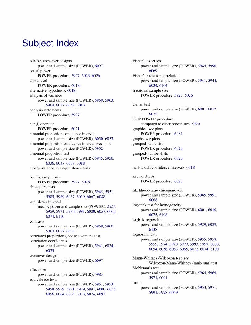
Subject Index
AB/BA crossover designspower and sample size (POWER), 6097
actual powerPOWER procedure, 5927, 6023, 6026
alpha levelPOWER procedure, 6018
alternative hypothesis, 6018analysis of variance
power and sample size (POWER), 5959, 5963,5964, 6057, 6058, 6083
analysis statementsPOWER procedure, 5927
bar (|) operatorPOWER procedure, 6021
binomial proportion confidence intervalpower and sample size (POWER), 6050–6053
binomial proportion confidence interval precisionpower and sample size (POWER), 5952
binomial proportion testpower and sample size (POWER), 5945, 5950,
6036, 6037, 6039, 6088bioequivalence, see equivalence tests
ceiling sample sizePOWER procedure, 5927, 6026
chi-square testspower and sample size (POWER), 5945, 5951,
5985, 5989, 6037, 6039, 6067, 6088confidence intervals
means, power and sample size (POWER), 5953,5959, 5971, 5980, 5991, 6000, 6057, 6065,6074, 6110
contrastspower and sample size (POWER), 5959, 5960,
5963, 6057, 6083correlated proportions, see McNemar’s testcorrelation coefficients
power and sample size (POWER), 5941, 6034,6035
crossover designspower and sample size (POWER), 6097
effect sizepower and sample size (POWER), 5983
equivalence testspower and sample size (POWER), 5951, 5953,
5958, 5959, 5971, 5979, 5991, 6000, 6055,6056, 6064, 6065, 6073, 6074, 6097
Fisher’s exact testpower and sample size (POWER), 5985, 5990,
6069Fisher’s z test for correlation
power and sample size (POWER), 5941, 5944,6034, 6104
fractional sample sizePOWER procedure, 5927, 6026
Gehan testpower and sample size (POWER), 6001, 6012,
6075GLMPOWER procedure
compared to other procedures, 5920graphics, see plots
POWER procedure, 6081graphs, see plotsgrouped-name-lists
POWER procedure, 6020grouped-number-lists
POWER procedure, 6020
half-width, confidence intervals, 6018
keyword-listsPOWER procedure, 6020
likelihood-ratio chi-square testpower and sample size (POWER), 5985, 5991,
6068log-rank test for homogeneity
power and sample size (POWER), 6001, 6010,6075, 6108
logistic regressionpower and sample size (POWER), 5929, 6029,
6138lognormal data
power and sample size (POWER), 5955, 5958,5959, 5974, 5978, 5979, 5993, 5999, 6000,6054, 6056, 6063, 6065, 6072, 6074, 6100
Mann-Whitney-Wilcoxon test, seeWilcoxon-Mann-Whitney (rank-sum) test
McNemar’s testpower and sample size (POWER), 5964, 5969,
5971, 6061means
power and sample size (POWER), 5953, 5971,5991, 5998, 6069

name-listsPOWER procedure, 6020
nominal powerPOWER procedure, 5927, 6023, 6026
noninferiority testspower and sample size (POWER), 5952, 6100
nonparametric testspower and sample size (POWER), 6013, 6017
null hypothesis, 6018number-lists
POWER procedure, 6020
odds ratiopower and sample size (POWER), 5985, 5989,
6066, 6067ODS graph names
POWER procedure, 6081ODS Graphics
POWER procedure, 6081one-sample t-test
power and sample size (POWER), 5920, 5953,5958, 6054, 6055
one-way ANOVApower and sample size (POWER), 5959, 5963,
5964, 6057, 6058, 6083
paired proportions, see McNemar’s testpaired t test
power and sample size (POWER), 5971, 5978,6062, 6063
paired-difference t test, see paired t testpartial correlations
power and sample size (POWER), 5941, 5944,6034, 6035, 6104
Pearson chi-square testpower and sample size (POWER), 5985, 5989,
6067Pearson correlation statistics
power and sample size (POWER), 5941, 6034,6035, 6104
plotspower and sample size (POWER), 5919, 5927,
5929, 5980, 6114power
overview of power concepts (POWER), 6018See POWER procedure, 5918
power curves, see plotsPOWER procedure
AB/BA crossover designs, 6097actual alpha, 6026actual power, 5927, 6023, 6026actual prob(width), 6026analysis of variance, 5959, 5963, 5964, 6057,
6058, 6083
analysis statements, 5927bar (|) operator, 6021binomial proportion confidence interval,
6050–6053binomial proportion confidence interval
precision, 5952binomial proportion tests, 5945, 5950, 6036,
6037, 6039, 6088ceiling sample size, 5927, 6026compared to other procedures, 5920computational methods, 6027computational resources, 6027confidence intervals for means, 5953, 5959,
5971, 5980, 5991, 6000, 6057, 6065, 6074,6110
contrasts, analysis of variance, 5959, 5960, 5963,6057, 6083
correlated proportions, 5964, 5969, 5971, 6061correlation, 5941, 6034, 6035, 6104crossover designs, 6097displayed output, 6026effect size, 5983equivalence tests, 5951, 5953, 5958, 5959, 5971,
5979, 5991, 6000, 6055, 6056, 6064, 6065,6073, 6074, 6097
Fisher’s exact test, 5985, 5990, 6069Fisher’s z test for correlation, 5941, 5944, 6034,
6104fractional sample size, 5927, 6026Gehan test, 6001, 6012, 6075graphics, 6081grouped-name-lists, 6020grouped-number-lists, 6020introductory example, 5920keyword-lists, 6020likelihood-ratio chi-square test, 5985, 5991, 6068log-rank test for comparing survival curves,
6001, 6010, 6075, 6108logistic regression, 5929, 6029, 6138lognormal data, 5955, 5958, 5959, 5974, 5978,
5979, 5993, 5999, 6000, 6054, 6056, 6063,6065, 6072, 6074, 6100
McNemar’s test, 5964, 5969, 5971, 6061name-lists, 6020nominal power, 5927, 6023, 6026noninferiority tests, 5952, 6100notation for formulas, 6027number-lists, 6020odds ratio, 5985, 5989, 6066, 6067ODS graph names, 6081ODS Graphics, 6081ODS table names, 6026one-sample t test, 5920, 5953, 5958, 6054

one-way ANOVA, 5959, 5963, 5964, 6057,6058, 6083
overview of power concepts, 6018paired proportions, 5964, 5969, 5971, 6061paired t test, 5971, 5978, 6062, 6063partial correlation, 5941, 5944, 6034, 6035, 6104Pearson chi-square test, 5985, 5989, 6067Pearson correlation, 5941, 5944, 6034, 6035,
6104plots, 5919, 5927, 5929, 5980, 6114regression, 5936, 5940, 6032, 6104relative risk, 5985, 5989, 6066, 6067sample size adjustment, 6023statistical graphics, 6081summary of analyses, 6018summary of statements, 5928superiority tests, 5952survival analysis, 6001, 6010, 6075t test for correlation, 5941, 5944, 6035t tests, 5953, 5958, 5971, 5978, 5991, 5998,
6054, 6062, 6069, 6072, 6114Tarone-Ware test, 6001, 6012, 6075two-sample t test, 5923, 5991, 5998, 5999, 6069,
6071, 6072, 6114value lists, 6020Wilcoxon-Mann-Whitney (rank-sum) test, 6013,
6017, 6079Wilcoxon-Mann-Whitney test, 6140z test, 5945, 5951, 6037, 6039
precision, confidence intervals, 6018prospective power, 5919
rank-sum test, see Wilcoxon-Mann-Whitney(rank-sum) test
regressionpower and sample size (POWER), 5936, 5940,
6032, 6104relative risk
power and sample size (POWER), 5985, 5989,6066, 6067
retrospective power, 5919
sample sizeoverview of power concepts (POWER), 6018See POWER procedure, 5918
sample size adjustmentPOWER procedure, 6023
Satterthwaite t testpower and sample size (POWER), 5991, 5999,
6071sawtooth power function, 6088statistical graphics
POWER procedure, 6081superiority tests
power and sample size (POWER), 5952survival analysis
power and sample size (POWER), 6001, 6010,6075
t testpower and sample size (POWER), 5953, 5958,
5971, 5978, 5991, 5998, 6054, 6062, 6069t test for correlation
power and sample size (POWER), 5941, 5944,6035
Tarone-Ware test for homogeneitypower and sample size (POWER), 6001, 6012,
6075two-sample t-test
power and sample size (POWER), 5923, 5991,5998, 5999, 6069, 6071, 6072, 6114
Type I error, 6018Type II error, 6018
value listsPOWER procedure, 6020
Welch t testpower and sample size (POWER), 5991, 5999,
6071width, confidence intervals, 6018Wilcoxon rank-sum test, see
Wilcoxon-Mann-Whitney (rank-sum) testWilcoxon-Mann-Whitney (rank-sum) test
power and sample size (POWER), 6013, 6079Wilcoxon-Mann-Whitney test
power and sample size (POWER), 6017, 6140
z testpower and sample size (POWER), 5945, 5951,
6037, 6039


Syntax Index
ACCRUALRATEPERGROUP= optionTWOSAMPLESURVIVAL statement
(POWER), 6002ACCRUALRATETOTAL= option
TWOSAMPLESURVIVAL statement(POWER), 6003
ACCRUALTIME= optionTWOSAMPLESURVIVAL statement
(POWER), 6003ALPHA= option
LOGISTIC statement (POWER), 5930MULTREG statement (POWER), 5937ONECORR statement (POWER), 5942ONESAMPLEFREQ statement (POWER), 5946ONESAMPLEMEANS statement (POWER),
5954ONEWAYANOVA statement (POWER), 5960PAIREDFREQ statement (POWER), 5965PAIREDMEANS statement (POWER), 5973TWOSAMPLEFREQ statement (POWER), 5986TWOSAMPLEMEANS statement (POWER),
5993TWOSAMPLESURVIVAL statement
(POWER), 6003TWOSAMPLEWILCOXON statement
(POWER), 6014
CI= optionONESAMPLEFREQ statement (POWER), 5946ONESAMPLEMEANS statement (POWER),
5954PAIREDMEANS statement (POWER), 5973TWOSAMPLEMEANS statement (POWER),
5993CONTRAST= option
ONEWAYANOVA statement (POWER), 5960CORR= option
LOGISTIC statement (POWER), 5930ONECORR statement (POWER), 5942PAIREDFREQ statement (POWER), 5965PAIREDMEANS statement (POWER), 5973
COVARIATES= optionLOGISTIC statement (POWER), 5930
COVODDSRATIOS= optionLOGISTIC statement (POWER), 5930
COVREGCOEFFS= optionLOGISTIC statement (POWER), 5931
CURVE= option
TWOSAMPLESURVIVAL statement(POWER), 6003
CV= optionONESAMPLEMEANS statement (POWER),
5955PAIREDMEANS statement (POWER), 5973TWOSAMPLEMEANS statement (POWER),
5993
DEFAULTNBINS= optionLOGISTIC statement (POWER), 5931
DEFAULTUNIT= optionLOGISTIC statement (POWER), 5931
DESCRIPTION= optionPLOT statement (POWER), 5984
DISCPROPDIFF= optionPAIREDFREQ statement (POWER), 5966
DISCPROPORTIONS= optionPAIREDFREQ statement (POWER), 5966
DISCPROPRATIO= optionPAIREDFREQ statement (POWER), 5966
DIST= optionONECORR statement (POWER), 5942ONESAMPLEMEANS statement (POWER),
5955PAIREDFREQ statement (POWER), 5966PAIREDMEANS statement (POWER), 5974TWOSAMPLEMEANS statement (POWER),
5993
EQUIVBOUNDS= optionONESAMPLEFREQ statement (POWER), 5947
EVENTSTOTAL= optionTWOSAMPLESURVIVAL statement
(POWER), 6004
FOLLOWUPTIME= optionTWOSAMPLESURVIVAL statement
(POWER), 6004
GROUPACCRUALRATES= optionTWOSAMPLESURVIVAL statement
(POWER), 6005GROUPLOSS= option
TWOSAMPLESURVIVAL statement(POWER), 6005
GROUPLOSSEXPHAZARDS= optionTWOSAMPLESURVIVAL statement
(POWER), 6005

GROUPMEANS= optionONEWAYANOVA statement (POWER), 5961TWOSAMPLEMEANS statement (POWER),
5994GROUPMEDLOSSTIMES= option
TWOSAMPLESURVIVAL statement(POWER), 6005
GROUPMEDSURVTIMES= optionTWOSAMPLESURVIVAL statement
(POWER), 6005GROUPNS= option
ONEWAYANOVA statement (POWER), 5961TWOSAMPLEFREQ statement (POWER), 5986TWOSAMPLEMEANS statement (POWER),
5994TWOSAMPLESURVIVAL statement
(POWER), 6006TWOSAMPLEWILCOXON statement
(POWER), 6014GROUPPROPORTIONS= option
TWOSAMPLEFREQ statement (POWER), 5986GROUPSTDDEVS= option
TWOSAMPLEMEANS statement (POWER),5994
GROUPSURVEXPHAZARDS= optionTWOSAMPLESURVIVAL statement
(POWER), 6006GROUPSURVIVAL= option
TWOSAMPLESURVIVAL statement(POWER), 6006
GROUPWEIGHTS= optionONEWAYANOVA statement (POWER), 5961TWOSAMPLEFREQ statement (POWER), 5986TWOSAMPLEMEANS statement (POWER),
5994TWOSAMPLESURVIVAL statement
(POWER), 6006TWOSAMPLEWILCOXON statement
(POWER), 6014
HALFWIDTH= optionONESAMPLEFREQ statement (POWER), 5947ONESAMPLEMEANS statement (POWER),
5955PAIREDMEANS statement (POWER), 5974TWOSAMPLEMEANS statement (POWER),
5994HAZARDRATIO= option
TWOSAMPLESURVIVAL statement(POWER), 6006
INTERCEPT= optionLOGISTIC statement (POWER), 5931
INTERPOL= option
PLOT statement (POWER), 5981
KEY= optionPLOT statement (POWER), 5981
LOGISTIC statementPOWER procedure, 5929
LOWER= optionONESAMPLEFREQ statement (POWER), 5947ONESAMPLEMEANS statement (POWER),
5955PAIREDMEANS statement (POWER), 5974TWOSAMPLEMEANS statement (POWER),
5994
MARGIN= optionONESAMPLEFREQ statement (POWER), 5947
MARKERS= optionPLOT statement (POWER), 5981
MAX= optionPLOT statement (POWER), 5982
MEAN= optionONESAMPLEMEANS statement (POWER),
5955MEANDIFF= option
PAIREDMEANS statement (POWER), 5974TWOSAMPLEMEANS statement (POWER),
5995MEANRATIO= option
PAIREDMEANS statement (POWER), 5974TWOSAMPLEMEANS statement (POWER),
5995METHOD= option
ONESAMPLEFREQ statement (POWER), 5948PAIREDFREQ statement (POWER), 5966
MIN= optionPLOT statement (POWER), 5982
MODEL= optionMULTREG statement (POWER), 5938ONECORR statement (POWER), 5942
MULTREG statementPOWER procedure, 5936
NAME= optionPLOT statement (POWER), 5984
NBINS= optionLOGISTIC statement (POWER), 5932TWOSAMPLEWILCOXON statement
(POWER), 6014NFRACTIONAL option
LOGISTIC statement (POWER), 5932MULTREG statement (POWER), 5938ONECORR statement (POWER), 5943ONESAMPLEMEANS statement (POWER),
5955

ONEWAYANOVA statement (POWER), 5961PAIREDFREQ statement (POWER), 5966PAIREDMEANS statement (POWER), 5974TWOSAMPLEFREQ statement (POWER), 5987TWOSAMPLEMEANS statement (POWER),
5995TWOSAMPLESURVIVAL statement
(POWER), 6006NFRACTIONAL= option
ONESAMPLEFREQ statement (POWER), 5948TWOSAMPLEWILCOXON statement
(POWER), 6015NFULLPREDICTORS= option
MULTREG statement (POWER), 5938NOINT option
MULTREG statement (POWER), 5938NPAIRS= option
PAIREDFREQ statement (POWER), 5966PAIREDMEANS statement (POWER), 5974
NPARTIALVARS= optionONECORR statement (POWER), 5943
NPERGROUP= optionONEWAYANOVA statement (POWER), 5961TWOSAMPLEFREQ statement (POWER), 5987TWOSAMPLEMEANS statement (POWER),
5995TWOSAMPLESURVIVAL statement
(POWER), 6007TWOSAMPLEWILCOXON statement
(POWER), 6015NPOINTS= option
PLOT statement (POWER), 5982NREDUCEDPREDICTORS= option
MULTREG statement (POWER), 5938NSUBINTERVAL= option
TWOSAMPLESURVIVAL statement(POWER), 6007
NTESTPREDICTORS= optionMULTREG statement (POWER), 5938
NTOTAL= optionLOGISTIC statement (POWER), 5932MULTREG statement (POWER), 5939ONECORR statement (POWER), 5943ONESAMPLEFREQ statement (POWER), 5948ONESAMPLEMEANS statement (POWER),
5955ONEWAYANOVA statement (POWER), 5961TWOSAMPLEFREQ statement (POWER), 5987TWOSAMPLEMEANS statement (POWER),
5995TWOSAMPLESURVIVAL statement
(POWER), 6007TWOSAMPLEWILCOXON statement
(POWER), 6015
NULLCONTRAST= optionONEWAYANOVA statement (POWER), 5961
NULLCORR= optionONECORR statement (POWER), 5943
NULLDIFF= optionPAIREDMEANS statement (POWER), 5974TWOSAMPLEMEANS statement (POWER),
5995NULLDISCPROPRATIO= option
PAIREDFREQ statement (POWER), 5967NULLMEAN= option
ONESAMPLEMEANS statement (POWER),5955
NULLODDSRATIO= optionTWOSAMPLEFREQ statement (POWER), 5987
NULLPROPORTION= optionONESAMPLEFREQ statement (POWER), 5948
NULLPROPORTIONDIFF= optionTWOSAMPLEFREQ statement (POWER), 5987
NULLRATIO= optionPAIREDMEANS statement (POWER), 5975TWOSAMPLEMEANS statement (POWER),
5995NULLRELATIVERISK= option
TWOSAMPLEFREQ statement (POWER), 5987
ODDSRATIO= optionPAIREDFREQ statement (POWER), 5967TWOSAMPLEFREQ statement (POWER), 5987
ONECORR statementPOWER procedure, 5941
ONESAMPLEFREQ statementPOWER procedure, 5945
ONESAMPLEMEANS statementPOWER procedure, 5953
ONEWAYANOVA statementPOWER procedure, 5959
OUTPUTORDER= optionLOGISTIC statement (POWER), 5932MULTREG statement (POWER), 5939ONECORR statement (POWER), 5943ONESAMPLEFREQ statement (POWER), 5948ONESAMPLEMEANS statement (POWER),
5956ONEWAYANOVA statement (POWER), 5962PAIREDFREQ statement (POWER), 5967PAIREDMEANS statement (POWER), 5975TWOSAMPLEFREQ statement (POWER), 5987TWOSAMPLEMEANS statement (POWER),
5995TWOSAMPLESURVIVAL statement
(POWER), 6007TWOSAMPLEWILCOXON statement
(POWER), 6015

PAIREDCVS= optionPAIREDMEANS statement (POWER), 5975
PAIREDFREQ statementPOWER procedure, 5964
PAIREDMEANS statementPOWER procedure, 5971
PAIREDMEANS= optionPAIREDMEANS statement (POWER), 5976
PAIREDPROPORTIONS= optionPAIREDFREQ statement (POWER), 5968
PAIREDSTDDEVS= optionPAIREDMEANS statement (POWER), 5976
PARTIALCORR= optionMULTREG statement (POWER), 5939
PLOT statementPOWER procedure, 5980
PLOTONLY= optionPROC POWER statement, 5929
POWER proceduresyntax, 5927
POWER procedure, LOGISTIC statement, 5929ALPHA= option, 5930CORR= option, 5930COVARIATES= option, 5930COVODDSRATIOS= option, 5930COVREGCOEFFS= option, 5931DEFAULTNBINS= option, 5931DEFAULTUNIT= option, 5931INTERCEPT= option, 5931NBINS= option, 5932NFRACTIONAL option, 5932NTOTAL= option, 5932OUTPUTORDER= option, 5932POWER= option, 5933RESPONSEPROB= option, 5933TEST= option, 5933TESTODDSRATIO= option, 5933TESTPREDICTOR= option, 5933TESTREGCOEFF= option, 5933UNITS= option, 5933VARDIST= option, 5934
POWER procedure, MULTREG statement, 5936ALPHA= option, 5937MODEL= option, 5938NFRACTIONAL option, 5938NFULLPREDICTORS= option, 5938NOINT option, 5938NREDUCEDPREDICTORS= option, 5938NTESTPREDICTORS= option, 5938NTOTAL= option, 5939OUTPUTORDER= option, 5939PARTIALCORR= option, 5939POWER= option, 5939RSQUAREDIFF= option, 5939
RSQUAREFULL= option, 5940RSQUAREREDUCED= option, 5940TEST= option, 5940
POWER procedure, ONECORR statement, 5941ALPHA= option, 5942CORR= option, 5942DIST= option, 5942MODEL= option, 5942NFRACTIONAL option, 5943NPARTIALVARS= option, 5943NTOTAL= option, 5943NULLCORR= option, 5943OUTPUTORDER= option, 5943POWER= option, 5944SIDES= option, 5944TEST= option, 5944
POWER procedure, ONESAMPLEFREQ statement,5945
ALPHA= option, 5946CI= option, 5946EQUIVBOUNDS= option, 5947HALFWIDTH= option, 5947LOWER= option, 5947MARGIN= option, 5947METHOD= option, 5948NFRACTIONAL= option, 5948NTOTAL= option, 5948NULLPROPORTION= option, 5948OUTPUTORDER= option, 5948POWER= option, 5949PROBWIDTH= option, 5949PROPORTION= option, 5949SIDES= option, 5949TEST= option, 5949UPPER= option, 5950VAREST= option, 5950
POWER procedure, ONESAMPLEMEANSstatement, 5953
ALPHA= option, 5954CI= option, 5954CV= option, 5955DIST= option, 5955HALFWIDTH= option, 5955LOWER= option, 5955MEAN= option, 5955NFRACTIONAL option, 5955NTOTAL= option, 5955NULLMEAN= option, 5955OUTPUTORDER= option, 5956POWER= option, 5956PROBTYPE= option, 5956PROBWIDTH= option, 5957SIDES= option, 5957STDDEV= option, 5957

TEST= option, 5957UPPER= option, 5957
POWER procedure, ONEWAYANOVA statement,5959
ALPHA= option, 5960CONTRAST= option, 5960GROUPMEANS= option, 5961GROUPNS= option, 5961GROUPWEIGHTS= option, 5961NFRACTIONAL option, 5961NPERGROUP= option, 5961NTOTAL= option, 5961NULLCONTRAST= option, 5961OUTPUTORDER= option, 5962POWER= option, 5962SIDES= option, 5962STDDEV= option, 5962TEST= option, 5963
POWER procedure, PAIREDFREQ statement, 5964ALPHA= option, 5965CORR= option, 5965DISCPROPDIFF= option, 5966DISCPROPORTIONS= option, 5966DISCPROPRATIO= option, 5966DIST= option, 5966METHOD= option, 5966NFRACTIONAL option, 5966NPAIRS= option, 5966NULLDISCPROPRATIO= option, 5967ODDSRATIO= option, 5967OUTPUTORDER= option, 5967PAIREDPROPORTIONS= option, 5968POWER= option, 5968PROPORTIONDIFF= option, 5968REFPROPORTION= option, 5968RELATIVERISK= option, 5968SIDES= option, 5968TEST= option, 5968TOTALPROPDISC= option, 5969
POWER procedure, PAIREDMEANS statement,5971
ALPHA= option, 5973CI= option, 5973CORR= option, 5973CV= option, 5973DIST= option, 5974HALFWIDTH= option, 5974LOWER= option, 5974MEANDIFF= option, 5974MEANRATIO= option, 5974NFRACTIONAL option, 5974NPAIRS= option, 5974NULLDIFF= option, 5974NULLRATIO= option, 5975
OUTPUTORDER= option, 5975PAIREDCVS= option, 5975PAIREDMEANS= option, 5976PAIREDSTDDEVS= option, 5976POWER= option, 5976PROBTYPE= option, 5976PROBWIDTH= option, 5976SIDES= option, 5976STDDEV= option, 5977TEST= option, 5977UPPER= option, 5977
POWER procedure, PLOT statement, 5980DESCRIPTION= option, 5984INTERPOL= option, 5981KEY= option, 5981MARKERS= option, 5981MAX= option, 5982MIN= option, 5982NAME= option, 5984NPOINTS= option, 5982STEP= option, 5982VARY option, 5982X= option, 5982XOPTS= option, 5983Y= option, 5984YOPTS= option, 5984
POWER procedure, PROC POWER statement, 5929PLOTONLY= option, 5929
POWER procedure, TWOSAMPLEFREQ statement,5985
ALPHA= option, 5986GROUPNS= option, 5986GROUPPROPORTIONS= option, 5986GROUPWEIGHTS= option, 5986NFRACTIONAL option, 5987NPERGROUP= option, 5987NTOTAL= option, 5987NULLODDSRATIO= option, 5987NULLPROPORTIONDIFF= option, 5987NULLRELATIVERISK= option, 5987ODDSRATIO= option, 5987OUTPUTORDER= option, 5987POWER= option, 5988PROPORTIONDIFF= option, 5988REFPROPORTION= option, 5988RELATIVERISK= option, 5988SIDES= option, 5988TEST= option, 5989
POWER procedure, TWOSAMPLEMEANSstatement, 5991
ALPHA= option, 5993CI= option, 5993CV= option, 5993DIST= option, 5993

GROUPMEANS= option, 5994GROUPNS= option, 5994GROUPSTDDEVS= option, 5994GROUPWEIGHTS= option, 5994HALFWIDTH= option, 5994LOWER= option, 5994MEANDIFF= option, 5995MEANRATIO= option, 5995NFRACTIONAL option, 5995NPERGROUP= option, 5995NTOTAL= option, 5995NULLDIFF= option, 5995NULLRATIO= option, 5995OUTPUTORDER= option, 5995POWER= option, 5996PROBTYPE= option, 5996PROBWIDTH= option, 5997SIDES= option, 5997STDDEV= option, 5997TEST= option, 5997UPPER= option, 5998
POWER procedure, TWOSAMPLESURVIVALstatement, 6001
ACCRUALRATEPERGROUP= option, 6002ACCRUALRATETOTAL= option, 6003ACCRUALTIME= option, 6003ALPHA= option, 6003CURVE= option, 6003EVENTSTOTAL= option, 6004FOLLOWUPTIME= option, 6004GROUPACCRUALRATES= option, 6005GROUPLOSS= option, 6005GROUPLOSSEXPHAZARDS= option, 6005GROUPMEDLOSSTIMES= option, 6005GROUPMEDSURVTIMES= option, 6005GROUPNS= option, 6006GROUPSURVEXPHAZARDS= option, 6006GROUPSURVIVAL= option, 6006GROUPWEIGHTS= option, 6006HAZARDRATIO= option, 6006NFRACTIONAL option, 6006NPERGROUP= option, 6007NSUBINTERVAL= option, 6007NTOTAL= option, 6007OUTPUTORDER= option, 6007POWER= option, 6008REFSURVEXPHAZARD= option, 6008REFSURVIVAL= option, 6008SIDES= option, 6008TEST= option, 6008TOTALTIME= option, 6009
POWER procedure, TWOSAMPLEWILCOXONstatement, 6013
ALPHA= option, 6014
GROUPNS= option, 6014GROUPWEIGHTS= option, 6014NBINS= option, 6014NFRACTIONAL= option, 6015NPERGROUP= option, 6015NTOTAL= option, 6015OUTPUTORDER= option, 6015POWER= option, 6015SIDES= option, 6016TEST= option, 6016VARDIST= option, 6016VARIABLES= option, 6017
POWER= optionLOGISTIC statement (POWER), 5933MULTREG statement (POWER), 5939ONECORR statement (POWER), 5944ONESAMPLEFREQ statement (POWER), 5949ONESAMPLEMEANS statement (POWER),
5956ONEWAYANOVA statement (POWER), 5962PAIREDFREQ statement (POWER), 5968PAIREDMEANS statement (POWER), 5976TWOSAMPLEFREQ statement (POWER), 5988TWOSAMPLEMEANS statement (POWER),
5996TWOSAMPLESURVIVAL statement
(POWER), 6008TWOSAMPLEWILCOXON statement
(POWER), 6015PROBTYPE= option
ONESAMPLEMEANS statement (POWER),5956
PAIREDMEANS statement (POWER), 5976TWOSAMPLEMEANS statement (POWER),
5996PROBWIDTH= option
ONESAMPLEFREQ statement (POWER), 5949ONESAMPLEMEANS statement (POWER),
5957PAIREDMEANS statement (POWER), 5976TWOSAMPLEMEANS statement (POWER),
5997PROC POWER statement, see POWER procedurePROPORTION= option
ONESAMPLEFREQ statement (POWER), 5949PROPORTIONDIFF= option
PAIREDFREQ statement (POWER), 5968TWOSAMPLEFREQ statement (POWER), 5988
REFPROPORTION= optionPAIREDFREQ statement (POWER), 5968TWOSAMPLEFREQ statement (POWER), 5988
REFSURVEXPHAZARD= option
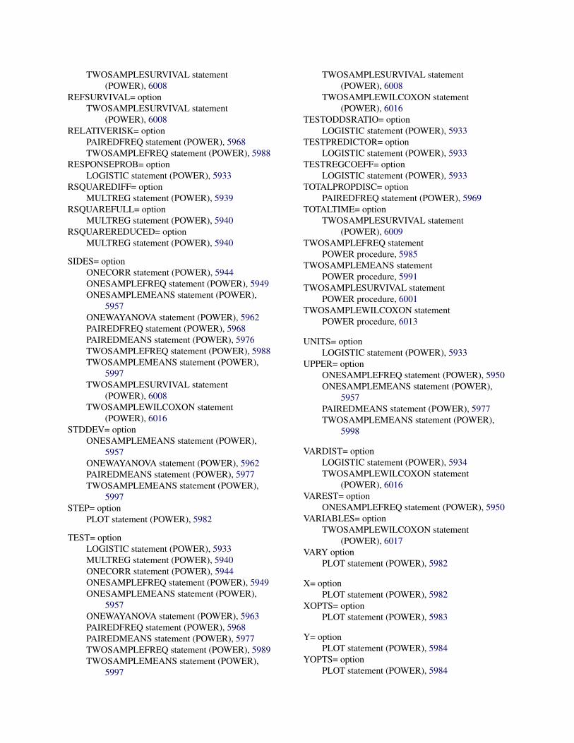
TWOSAMPLESURVIVAL statement(POWER), 6008
REFSURVIVAL= optionTWOSAMPLESURVIVAL statement
(POWER), 6008RELATIVERISK= option
PAIREDFREQ statement (POWER), 5968TWOSAMPLEFREQ statement (POWER), 5988
RESPONSEPROB= optionLOGISTIC statement (POWER), 5933
RSQUAREDIFF= optionMULTREG statement (POWER), 5939
RSQUAREFULL= optionMULTREG statement (POWER), 5940
RSQUAREREDUCED= optionMULTREG statement (POWER), 5940
SIDES= optionONECORR statement (POWER), 5944ONESAMPLEFREQ statement (POWER), 5949ONESAMPLEMEANS statement (POWER),
5957ONEWAYANOVA statement (POWER), 5962PAIREDFREQ statement (POWER), 5968PAIREDMEANS statement (POWER), 5976TWOSAMPLEFREQ statement (POWER), 5988TWOSAMPLEMEANS statement (POWER),
5997TWOSAMPLESURVIVAL statement
(POWER), 6008TWOSAMPLEWILCOXON statement
(POWER), 6016STDDEV= option
ONESAMPLEMEANS statement (POWER),5957
ONEWAYANOVA statement (POWER), 5962PAIREDMEANS statement (POWER), 5977TWOSAMPLEMEANS statement (POWER),
5997STEP= option
PLOT statement (POWER), 5982
TEST= optionLOGISTIC statement (POWER), 5933MULTREG statement (POWER), 5940ONECORR statement (POWER), 5944ONESAMPLEFREQ statement (POWER), 5949ONESAMPLEMEANS statement (POWER),
5957ONEWAYANOVA statement (POWER), 5963PAIREDFREQ statement (POWER), 5968PAIREDMEANS statement (POWER), 5977TWOSAMPLEFREQ statement (POWER), 5989TWOSAMPLEMEANS statement (POWER),
5997
TWOSAMPLESURVIVAL statement(POWER), 6008
TWOSAMPLEWILCOXON statement(POWER), 6016
TESTODDSRATIO= optionLOGISTIC statement (POWER), 5933
TESTPREDICTOR= optionLOGISTIC statement (POWER), 5933
TESTREGCOEFF= optionLOGISTIC statement (POWER), 5933
TOTALPROPDISC= optionPAIREDFREQ statement (POWER), 5969
TOTALTIME= optionTWOSAMPLESURVIVAL statement
(POWER), 6009TWOSAMPLEFREQ statement
POWER procedure, 5985TWOSAMPLEMEANS statement
POWER procedure, 5991TWOSAMPLESURVIVAL statement
POWER procedure, 6001TWOSAMPLEWILCOXON statement
POWER procedure, 6013
UNITS= optionLOGISTIC statement (POWER), 5933
UPPER= optionONESAMPLEFREQ statement (POWER), 5950ONESAMPLEMEANS statement (POWER),
5957PAIREDMEANS statement (POWER), 5977TWOSAMPLEMEANS statement (POWER),
5998
VARDIST= optionLOGISTIC statement (POWER), 5934TWOSAMPLEWILCOXON statement
(POWER), 6016VAREST= option
ONESAMPLEFREQ statement (POWER), 5950VARIABLES= option
TWOSAMPLEWILCOXON statement(POWER), 6017
VARY optionPLOT statement (POWER), 5982
X= optionPLOT statement (POWER), 5982
XOPTS= optionPLOT statement (POWER), 5983
Y= optionPLOT statement (POWER), 5984
YOPTS= optionPLOT statement (POWER), 5984


Your Turn
We welcome your feedback.
� If you have comments about this book, please send them [email protected]. Include the full title and page numbers (if applicable).
� If you have comments about the software, please send them [email protected].


SAS® Publishing Delivers!Whether you are new to the work force or an experienced professional, you need to distinguish yourself in this rapidly changing and competitive job market. SAS® Publishing provides you with a wide range of resources to help you set yourself apart. Visit us online at support.sas.com/bookstore.
SAS® Press Need to learn the basics? Struggling with a programming problem? You’ll find the expert answers that you need in example-rich books from SAS Press. Written by experienced SAS professionals from around the world, SAS Press books deliver real-world insights on a broad range of topics for all skill levels.
s u p p o r t . s a s . c o m / s a s p r e s sSAS® Documentation To successfully implement applications using SAS software, companies in every industry and on every continent all turn to the one source for accurate, timely, and reliable information: SAS documentation. We currently produce the following types of reference documentation to improve your work experience:
• Onlinehelpthatisbuiltintothesoftware.• Tutorialsthatareintegratedintotheproduct.• ReferencedocumentationdeliveredinHTMLandPDF– free on the Web. • Hard-copybooks.
s u p p o r t . s a s . c o m / p u b l i s h i n gSAS® Publishing News Subscribe to SAS Publishing News to receive up-to-date information about all new SAS titles, author podcasts, and new Web site features via e-mail. Complete instructions on how to subscribe, as well as access to past issues, are available at our Web site.
s u p p o r t . s a s . c o m / s p n
SAS and all other SAS Institute Inc. product or service names are registered trademarks or trademarks of SAS Institute Inc. in the USA and other countries. ® indicates USA registration. Otherbrandandproductnamesaretrademarksoftheirrespectivecompanies.©2009SASInstituteInc.Allrightsreserved.518177_1US.0109