1. INTRODUCTION TO STATISTICS 

The impact of statistics profoundly affects society today. Every day, we have confronted with some form of statistical information through news papers, magazines, and other forms of communication. Besides, statistical tables, survey results, and the language of probability are used with increasing frequency by the media. Such statistical information has become highly influential in our lives.

Statistics can be considered as numerical statements of facts which are highly convenient and meaningful forms of communication. The subjects of statistics, as it seems, is not a new discipline but it is as old as the human society itself. The sphere of its utility, however, was very much restricted. The word statistics is derived from the Latin word status which means a political state or government. It was originally applied in connection with kings and monarchs collecting data on their citizenry which pertained to state wealth, taxes collected population and so on. Thus, the scope of statistics in the ancient times was primarily limited to the collection of demographic and property and wealth data of a country by governments for framing military and fiscal policies.

Now days, statistics is used almost in every field of study, such as natural science, social science, engineering, medicine, agriculture, etc. The improvements in computer technology make it easier than ever to use statistical methods and to manipulate massive amounts of data.

Definition and Classification of Statistics Statistics as a subject (field of study): Statistics is defined as the science of collecting, organizing, presenting, analyzing and interpreting numerical data to make decision on the bases of such analysis.(Singular sense)

Statistics as a numerical data: Statistics is defined as aggregates of numerical expressed facts (figures) collected in a systematic manner for a predetermined purpose. (Plural sense) In this course, we shall be mainly concerned with statistics as a subject, that is, as a field of study. Classification of Statistics: Statistics is broadly divided into two categories based on how the collected data are used. i. Descriptive Statistics: is concerned with summary calculations, graphs, charts and

tables. It deals with describing data without attempting to infer anything that goes beyond the given set of data. It consists of collection, organization, summarization and presentation of data in the convenient and informative way.

Examples: • The amount of medication in blood pressure pills. • The starting salaries for Mathematics and Statistics students in different

organizations.

1  

ii. Inferential Statistics: Descriptive Statistics describe the data set that’s being analyzed, but doesn’t allow us to draw any conclusions or make any inferences about the data, other than visual “It looks like …..” type statements. It deals with making inferences and/or conclusions about a population based on data obtained from a limited sample of observations. It consists of performing hypothesis testing, determining relationships among variables and making predictions. For example, the average income of all families (the population) in Ethiopia can be estimated from figures obtained from a few hundred (the sample) families.

Examples:

a) From past figures, it has been predicted that 90 00 of registered voters will vote in the

November election. b) The average age of a student in Hawassa University is 19.1 years. c) To determine the most effective dose of a new medication (on the basis of tests

performed with volunteer patients from selected hospitals) d) To compare the effectiveness of two reducing diets (based on the weights losses of

persons who were taking the diets) e) There is a relationship between smoking tobacco and an increased risk of developing

cancer.

Stages of Statistical Investigation The area of statistics incorporates the following five stages. These are collection, organization, presentation, analysis and interpretation of data. Proper collection of data: Data can be collected in a variety of ways; one of the most common methods is through the use of survey. Survey can also be done in different methods, three of the most common methods are: Telephone survey, Mailed questionnaire, Personal interview. Organization of data: If an investigator has collected data through a survey, it is necessary to edit these data in order to correct any apparent inconsistencies, ambiguities, and recording errors. Presentation of data: the organized data can now be presented in the form of tables or diagrams or graphs. This presentation in an orderly manner facilitates the understanding as well as analysis of data. Analysis of data: the basic purpose of data analysis is to make it useful for certain conclusions. This analysis may simply be a critical observation of data to draw some meaningful conclusions about it or it may involve highly complex and sophisticated mathematical techniques. Interpretation of data: Interpretation means drawing conclusions from the data which form the basis of decision making. Correct interpretation requires a high degree of skill and experience and is necessary in order to draw valid conclusions.

2  

Definition of some basic terms Population: It is the totality of things under considerations. The population represents the target of an investigation, and the objective of the investigation is to draw conclusions about the population hence we sometimes call it target population. Examples:

• All university students of Ethiopia • Population of trees under specified climatic conditions • Population of animals fed a certain type of diet • Population of farms having a certain type of natural fertility • Population of households, etc

The population could be finite or infinite (an imaginary collection of units). There are two ways of investigation: Census and sample survey. Census: a complete enumeration of the population. But in most real problems it cannot be realized, hence we take sample. Sample: A group of subjects selected from a population. A sample from a population is the set of measurements that are actually collected in the course of an investigation. For example, if we want to study the income pattern of lecturers at Hawassa University and there are 3000 lecturers, then we may take a random sample of only 250 lecturers out of this entire population of 3000 for the purpose of study. Then this number of 250 lecturers constitutes a sample.

In practice, we rarely conduct census, instead we conduct sample survey Parameter: is a descriptive measure of a population, or summary value calculated from a population. Examples: Average, Range, proportion, variance, Statistic: is a descriptive measure of a sample, or summary value calculated from a sample. From the previous example, the summary measure that describes a characteristic such as average income of this sample is known as a statistic. Sampling: The process or method of sample selection from the population. Sample size: The number of elements or observation to be included in the sample. Variable: It is an item of interest that can take on many different numerical values.

Applications, Uses and Limitation of Statistics Applications of Statistics Statistics can be applied in any field of study which seeks quantitative evidence. For instance, engineering, economics, natural science, etc.

a) Engineering: Statistics have wide application in engineering. • To compare the breaking strength of two types of materials • To determine the probability of reliability of a product. • To control the quality of products in a given production process. • To compare the improvement of yield due to certain additives

(fertilizer, herbicides, (wee decides), e t c b) Economics: Statistics are widely used in economics study and research.

• To measure and forecast Gross National Product (GNP)

3  

• Statistical analyses of population growth, unemployment figures, rural or urban population shifts and so on influence much of the economic policy making

• Financial statistics are necessary in the fields of money and banking including consumer savings and credit availability.

c) Statistics and research: there is hardly any advanced research going on without the use of statistics in one form or another. Statistics are used extensively in medical, pharmaceutical and agricultural research.

Uses of Statistics Today the field of statistics is recognized as a highly useful tool to making decision process by managers of modern business, industry, frequently changing technology. It has a lot of functions in everyday activities. The following are some uses of statistics:

• Statistics condenses and summarizes complex data: the original set of data (raw data) is normally voluminous and disorganized unless it is summarized and expressed in few numerical values.

• Statistics facilitates comparison of data: measures obtained from different set of data can be compared to draw conclusion about those sets. Statistical values such as averages, percentages, ratios, etc, are the tools that can be used for the purpose of comparing sets of data.

• Statistics helps in predicting future trends: statistics is extremely useful for analyzing the past and present data and predicting some future trends.

• Statistics influences the policies of government: statistical study results in the areas of taxation, on unemployment rate, on the performance of every sort of military equipment, etc, may convince a government to review its policies and plans with the view to meet national needs and aspirations.

• Statistical methods are very helpful in formulating and testing hypothesis and to develop new theories.

Limitations of Statistics The field of statistics, though widely used in all areas of human knowledge and widely applied in a variety of disciplines such as business, economics and research, has its own limitations. Some of these limitations are:

a) It does not deal with individual values: as discussed earlier, statistics deals with aggregate of values. For example, the population size of a country for some given year does not help us for comparative studies, unless it can be compared with some other countries or with a set standard.

b) It does not deal with qualitative characteristics directly: statistics is not applicable to qualitative characteristics such as beauty, honesty, poverty, standard of living and so on since these cannot be expressed in quantitative terms. These characteristics, however, can be statistically dealt with if some quantitative values can be assigned to these with logical criterion. For

4  

c) Statistical conclusions are not universally true: since statistics is not an exact science, as is the case with natural sciences, the statistical conclusions are true only under certain assumptions. Also, the field deals extensively with the laws of probability which at best are educated guesses. For example, if we toss a coin 10 times where the chances of a head or a tail are 1:1, we cannot say with certainty that there will be 5 heads and 5 tails. Thus the statistical laws are only approximations.

d) It is sensitive for misuse: The famous statement that figures don’t lie but the liars can figure, is a testimony to the misuse of statistics. Thus inaccurate or incomplete figures can be manipulated to get desirable references. The number of car accidents committed in a city in a particular year by women drivers is 10 while that committed by men drivers is 40. Hence women drivers are safe drivers.

TYPES OF VARIABLES AND MEASUREMENT SCALES

Types of Variables A variable is a characteristic of an object that can have different possible values. Age, height, IQ and so on are all variables since their values can change when applied to different people. For example, Mr. X is a variable since X can represent anybody. A variable may be qualitative or quantitative in nature. These two types of variables are:

a) Quantitative variables: are variables that can be quantified or can have numerical values. Examples: height, area, income, temperature e t c. Consider the following questions; How many rooms are there in your house? Or How many children are there in the family? Would be in numerical values.

b) Qualitative variables: are variables that cannot be quantified directly. Examples: color, beauty, sex, location, political affiliation, and so on. Consider also the following questions; “are you currently unemployed?” Would fit in the category of either yes or no. Qualitative variables are also called categorical variables. And hence we have two types of data; quantitative & qualitative data.

Quantitative variables can be further classified as

Discrete variables, and Continuous variables

a) Discrete variables are variables whose values are counts. For examples: • number of students attending a conference • number of households (family size) • Number of pages of a book • number of eggs in the refrigerator, etc

b) Continuous variables are variables that can have any value within an interval.

5  

Examples: • height of models in a beauty context • weight of people joining a diet program • Lengths of steel bars in a given production terms, e t c.

Scales of Measurement Proper knowledge about the nature and type of data to be dealt with is essential in order to specify and apply the proper statistical method for their analysis and inferences. Measurement is the assignment of numbers to objects or events in a systematic 

fashion.  It is a functional mapping from the set of objects {Oi} to the set of real numbers {M(Oi)}

Measurement scale refers to the property of value assigned to the data based on the properties of order, distance and fixed zero. Four levels of measurement scales are commonly distinguished: nominal, ordinal, interval, and ratio and each possessed different properties of measurement systems 

Nominal scale: - “Nominal “is a Latin word for “name” which measures the presence or absence of a characteristic of the data. The values of a nominal attribute are just different names, i.e., nominal attributes provide only enough information to distinguish one object from another. Qualities with no ranking or ordering; no numerical or quantitative value. Data consists of names, labels and categories. This is a scale for grouping individuals into different categories.

Examples: Car colors for a certain model are: red, silver, blue and black.

• In this scale, one is different from the other • +, -, *, /, Impossible, comparison is impossible

Ordinal scale: - measures the presence or absence of a characteristic of the data using an implied ranking or order. “Ordinal” is a Latin word, meaning “order”.

• Can be arranged in some order, but the differences between the data values are meaningless.

• Data consisting of an ordering of ranking of measurements are said to be on an ordinal scale of measurements. That is, the values of an ordinal scale provide enough information to order objects. (<, >)

• One is different from and grater /better/ less than the other • +, -, *, / Are impossible, comparison is possible. Consider the following examples about ordinal scale:

a. Man A weighs more than man B b. Ethiopian athletes got 1st and 2nd ranks in the 10,000m women’s final

in Beijing. c. Of 17 fishing reels rated: 6 were rated good quality, 4 were rated better

quality, and 7 were rated best quality. d. Out of a high school class of 319, Walter ranked 4th, June ranked

12th, and Jim ranked 20th.

6  

Interval Level: Data values can be ranked and the differences between data values are meaningful. However, there is no intrinsic zero, or starting point, and the ratio of data values are meaningless. Note: Celsius & Fahrenheit temperature readings have no meaningful zero and ratios are meaningless.

In this measurement scale:- • One is different, better/greater by a certain amount of difference than another • Possible to add and subtract. For example; 37Oc –35oc = 2oc, 45oc – 43 oc= 2oc • Multiplication and division are not possible. For example; 40oc = 2(20oc) But

this does not imply that an object which is 40 oc is twice as hot as an object which is 20 oc

Interval scale data convey better information than nominal and ordinal scale. Most common examples are: IQ, temperature, Calendar dates, etc

Consider the following examples:

a. The years in which democrats won presidential elections. b. Body temperature in degrees Celsius (or Fahrenheit) c. Building A was built in 1284, Building B in 1492 and Building C in 5 B.C.

Ratio scale: Similar to interval, except there is a true zero, or starting point, and the ratios of data values have meaning.

Best type of data: can add, subtract, multiply and divide. For ratio variables, both differences and ratios are meaningful.

One is different, larger /taller/ better/ less by a certain amount of difference and so much times than the other.

This measurement scale provides better information than interval scale of measurement

Examples: temperature in Kelvin, monetary quantities, counts, age, mass, length, electric current. Consider the following some more examples:

a. Core temperatures of stars measures in degrees Kelvin b. Time elapsed between the deposit of a check and the clearance of that check. c. Length of the Nile River.

2. Methods of Data Collection and Presentation 

Methods of Data Collection Data: are the values (measurements or observations) that the variables can assume. Variables that are determined by chance are called random variables. Any aggregate of numbers cannot be called statistical data. We say an aggregate of numbers is statistical data when they are

• Comparable • Meaningful and • Collected for a well defined objective

Raw data: are collected data, which have not been organized numerically. Examples: 25, 10, 32, 18, 6, 93, 4.

7  

The required data can be obtained from either a primary source or a secondary source. Primary source: Is a source of data that supplies first hand information for the use of the immediate purpose. Primary Data: data you collect to answer your question. Data measured or collected by the investigator or the user directly from the source. Or data originally collected for the immediate purpose.

Two activities involved: planning and measuring. a) Planning:

• Identify source and elements of the data. • Decide whether to consider sample or census. • If sampling is preferred, decide on sample size, selection method,… etc • Decide measurement procedure. • Set up the necessary organizational structure.

b) Measuring: there are different options. • Focus Group • Telephone Interview • Mail Questionnaires • Door-to-Door Survey • Mall Intercept • New Product Registration • Personal Interview and • Experiments are some of the sources for collecting the primary data.

Secondary source: are individuals or agencies, which supply data originally collected for other purposes by them or others. Usually they are published or unpublished materials, records, reports, e t c.

Secondary data: data collected from a secondary source by other people for other purposes. Data gathered or compiled from published and unpublished sources or files. When our source is secondary data check that:

• The type and objective of the situations. • The purpose for which the data are collected and compatible with the present

problem. • The nature and classification of data is appropriate to our problem. • There are no biases and misreporting in the published data.

Note: Data which are primary for one may be secondary for the other.

Methods of Data Presentation Having collected and edited the data, the next important step is to organize it. That is to present it in a readily comprehensible condensed form that aids in order to draw inferences from it. It is also necessary that the like be separated from the unlike ones. The presentation of data is broadly classified in to the following two categories:

• Tabular presentation • Diagrammatic and Graphic presentation.

The process of arranging data in to classes or categories according to similarities technically is called classification. It eliminates inconsistency and also brings out the

8  

points of similarity and/or dissimilarity of collected items/data. It is necessary because it would not be possible to draw inferences and conclusions if we have a large set of collected [raw] data.

Frequency Distributions

Frequency: - is the number of times a certain value or set of values occurs in a specific group.

A frequency distribution is a table that presents data according to some criteria with the corresponding number of items falling in each class (i.e. with the corresponding frequencies.). We see at a glance the shape of the distribution, the range of variation, and any clustering of the values. By presenting a frequency distribution in relative form, i.e., as percentages, we convert to the familiar base of 100 and make it easy to compare the distribution of cases between different variables and/or different samples, each of which may involve different total numbers of cases.

Generally, there are three basic types of frequency distributions: Categorical, Ungrouped and Grouped frequency distributions. 1. Categorical frequency distribution

– the data are usually qualitative – the scales of measurements for the data are usually nominal or ordinal

For instance data on blood types of people, political affiliation, economic status (low, medium and high), religious affiliation are presented by categorical frequency distributions.

Example: Thirty students, last year, took Stat 100 course and their grades were as follows. Construct an appropriate frequency distribution for these data.

Table 2.1: Grades of students

B B C B A C

D C C C B B

B A B C D C

A F B F C A

B C C A C D

Solution: There are five kinds of grades: A, B, C, D and F which may be used as the classes for constructing the distribution. The procedure for constructing a frequency distribution for categorical data is given below.

STEP 1. Construct a table as shown below STEP 2. Tally the data and place the results STEP 3. Count the Tallies and put the results

9  

STEP 4. Calculate the percentages (%) of frequencies in each class ( ) 100% ×=nf

Where = frequency of the class = total number of observations f n

Class

( I )

Tally

( II )

Frequency

( III )

Percent*

( IV )

A ///// 5 16.7

B ///// //// 9 30.0

C ///// ///// / 11 36.7

D /// 3 10.0

F // 2 6.7

2. Ungrouped frequency distribution Ungrouped frequency distribution is a table of all potential raw scored values that could possibly occur in the data along with their corresponding frequencies. It is often constructed for small set of data or a discrete variable. Constructing an ungrouped frequency distribution To construct an ungrouped frequency distribution, first find the smallest and the largest raw scores in the collected data. Then make a columnar table of all potential raw scored values arranged in order of magnitude with the number of times a particular value is repeated, i.e., the frequency of that value. To facilitate counting method, tallies can be used. Example: The following data are the ages in years of 20 women who attend health education last year: 30, 41, 39, 41, 32, 29, 35, 31, 30, 36, 33, 36, 32, 42, 30, 35, 37, 32, 30, and 41. Construct a frequency distribution for these data.

Solution: STEP 1. Find the range: nobservatioMinimumnobservatioMaximumRange −= STEP 2. Construct a table, tally the data and complete the frequency column. The

frequency distribution becomes as follows.

Age 29 30 31 32 33 35 36 37 39 41 42 Tally / //// / /// / // // / / /// / Frequency 1 4 1 3 1 2 2 1 1 3 1

3. Grouped frequency distribution STEP 1. Determine the unit of measurement, U STEP 2. Find the maximum(Max) and the minimum(Min) observation, and then

compute their range, R MinMaxRange −= STEP 3. Fix the number of classes’ desired (k). there are two ways to fix k:

• Fix k arbitrarily between 6 and 20, or • Use Sturge’s Formula: Nk 10log332.31+= where N is the total frequency.

And round this value of k up to get an integer number.

10  

STEP 4. Find the class widths (W) by dividing the range by the number of classes and

round the number up to get an integer value. KRW =

STEP 5. Pick a suitable starting point less than or equal to the minimum value. This starting point is the lower limit of the first class. Continue to add the class width to this lower limit to get the rest of the lower limits.

STEP 6. Find the upper class limits. To find the upper class limit of the first class, subtract one unit of measurement from the lower limit of the second class. Then continue to add the class width to this upper limit to get the rest of the upper limits.

STEP 7. Compute the class boundaries as: ULCLLCB 21−= and UUCLUCB 2

1+= Where LCL = lower class limit, UCL= upper class limit, LCB= lower class boundary and UCB= upper class boundary. The class boundaries are also half way between the upper limit of one class and the lower limit of the next class.

STEP 8. Tally the data. STEP 9. Find the frequencies. STEP 10. (If necessary) Find the cumulative frequencies (more than and less than types). Example: The number of hours 40 employees spends on their job for the last 7 days

Table: Number of hours employees spend 62 50 35 36 31 43 43 43

41 31 65 30 41 58 49 41

37 62 27 47 65 50 45 48

27 53 40 29 63 34 44 32

58 61 38 41 26 50 47 37

Construct a suitable frequency distribution for these data using 8 classes Solution:

1. Unit of measurement; U= 1year 2. Max = 65, Min = 26 so that R = 65-26 = 39 3. It is already determined to construct a frequency distribution having 8 classes.

4. Class width 5875.4539 ≈==W

5. Starting point = 26 = lower limit of the first class. And hence the lower class limits become: 26 31 36 41 46 51 56 61

6. Upper limit of the first class = 31-1 = 30. And hence the upper class limits become 30 35 40 45 50 55 60 65

The lower and the upper class limits (Steps 5 and 6) can be written as follows. Class limits 26-30 31-35 36-40 41-45 46-50 51-55 56-60 61-65 7. By subtracting 0.5 units of measurement from the lower class limits and by

adding 0.5 units of measurement to the upper class limits, we can get lower and upper class boundaries as follows.

Class Boundaries

25.5-30.5

30.5-35.5

35.5-40.5

40.5-45.5

45.5-50.5

50.5-55.5

55.5-60.5

60.5-65.5

STEPS 8, 9 and 10 are displayed in the following table.

11  

Class limits Class boundaries

Tally frequency

Cumulative frequency (less than

type)

Cumulative frequency (more than

type) 26 – 30 25.5 – 30.5 ///// 5 5 40 31 – 35 30.5 – 35.5 ///// 5 10 35 36 – 40 35.5– 40.5 ///// 5 15 30 41 – 45 40.5– 45.5 ///// //// 9 24 25 46 – 50 45.5– 50.5 ///// // 7 31 16 51 – 55 50.5– 55.5 / 1 32 9 56 – 60 55.5– 60.5 // 2 34 8 61 – 65 60.5– 65.5 ///// / 6 40 6

Diagrammatic presentation of data: Bar charts, Pie-chart, Cartograms The most convenient and popular way of describing data is using graphical presentation. It is easier to understand and interpret data when they are presented graphically than using words or a frequency table. A graph can present data in a simple and clear way. Also it can illustrate the important aspects of the data. This leads to better analysis and presentation of the data.

What it is? Graphs are pictorial representations of the relationships between two (or more) variables and are an important part of descriptive statistics. Different types of graphs can be used for illustration purposes depending on the type of variable (nominal, ordinal, or interval) and the issues of interest. When to Use It? Graphs can be used any time one wants to visually summarize the relationships between variables, especially if the data set is large or unmanageable. They are routinely used in reports to underscore a particular statement about a data set and to enhance readability. Graphs can appeal to visual memory in ways that mere tallies, tables, or frequency distributions cannot. However, if not used carefully, graphs can misrepresent relationships between variables or encourage inaccurate conclusions. Importance:

• They have greater attraction. • They facilitate comparison. • They are easily understandable.

The three most commonly used diagrammatic presentation for discrete as well as qualitative data are: • Pie charts, • Pictogram, • Bar charts Pie chart A pie chart is a circle that is divided in to sections or wedges according to the percentage of frequencies in each category of the distribution. The angle of the sector is obtained using:

360* o

quantitywholetheparttheofValueSectorofAngle =

12  

Example The following data are the blood types of 50 volunteers at a blood plasma donation clinic: O A O AB A A O O B A O A AB B O O O A B A A O A A

O B A O AB A O O A B A A A O B O O A O A B O AB A O B a) Organize this data using a categorical frequency distribution b) Present the data using both a pie and a bar chart.

Solution a) The classes of the frequency distribution are A, B, O, AB. Count the number of

donors for each of the blood types.

Table: the number of donors by blood types.

Blood type Frequency Percent

A 19 38 B 8 16 O 19 38

AB 4 8 Total 50 100

b) Pie chart Find the percentage of donors for each blood type. In order to find the angles of the sector for each blood type, multiply the corresponding percentage by 3600

and divide by 100.

Figure: Pie-chart of the data on blood types of donors.

ABOBA

Blood type

Pictogram In these diagrams, we represent data by means of some picture symbols. We decide abut a suitable picture to represent a definite number of units in which the variable is measured Example: The following table shows the orange production in a plantation from production year 1990-1993. Represent the data by a pictogram. Solution: Table: Orange productions from 1990 to 1993

Production year 1990 1991 1992 1993

Amount (in kg) 3000 3850 3500 5000

13  

Figure: Pictogram of the data on Orange productions from 1990 to 1993. Bar Charts

Bar graphs are commonly used to show the number or proportion of nominal or ordinal data which possess a particular attribute. They depict the frequency of each category of data points as a bar rising vertically from the horizontal axis. Bar graphs most often represent the number of observations in a given category, such as the number of people in a sample falling into a given income or ethnic group. They can be used to show the proportion of such data points. Bar graphs are especially good for showing how nominal data change over time. They are useful for comparing aggregate over time space. Bars can be drawn either vertically or horizontally.

There are different types of bar charts. The most common being: Simple bar chart, Component or sub divided bar chart, and Multiple bar charts.

Simple Bar Chart: Are used to display data on one variable and are thick lines (narrow rectangles) having the same breadth.

Example: Suppose that the following were the gross revenues (in $100,000.00) for company XYZ for the years 1989, 1990 and 1991. Draw the bar graph for this data. Table: Gross revenue of companies

Year Revenue1989 110 1990 95 1991 65

Solution: The bar diagram for this data can be constructed as follows with the revenues represented on the vertical axis and the years represented on the horizontal axis.

199119901989

110

100

90

80

70

60

Year

Sum

of R

even

ue

14  

Component Bar chart When there is a desire to show how a total (or aggregate) is divided in to its component parts, we use component bar chart. The bars represent total value of a variable with each total broken in to its component parts and different colors or designs are used for identifications Example: Construct a sub-divided bar chart for the four types of products in relation to the opinion of consumers purchasing the given products as given below: Table: Opinion of consumers purchasing the given products Products Definitely Probably Unsure No Product 1 50% 40% 10% 2% Product 2 60% 30% 12% 15% Product 3 70% 45% 8% 8% Product 4 60% 35% 5% 20%

Component Bar Chart

0%

50%

100%

1 2 3 4

Products

Opi

nion

of

Cons

umer

s

NOUnsureProbablyDefinitely

Multiple Bar charts These are used to display data on more than one variable.

They are used for comparing different variables at the same time. Example: Construct a sub-divided bar chart for the 3 types of expenditures in dollars for a family of four for the years 1, 2, 3 and 4 as given below: Table: Expenditures in dollars for families Year Food Education Other Total 1 3000 2000 3000 8000 2 3500 3000 4000 10500 3 4000 3500 5000 12500 5000 5000 6000 16000

Bar Charts

02000400060008000

1 2 3 4

Year

Type

s of

ex

pend

iture

s

FoodEducationOtherTotal

Figure: Multiple bar chart for Expenditures in dollars for families

15  

Graphical presentation of data: Histogram, and Frequency Polygon The histogram, frequency polygon and cumulative frequency graph or ogives are most commonly applied graphical representation for continuous data. Procedures for constructing statistical graphs: • Draw and label the X and Y axes. • Choose a suitable scale for the (cumulative) frequencies and label it on the Y axes. • Represent the class boundaries for the histogram or ogive or the mid points for the

frequency polygon on the X axes. • Plot the points. • Draw the bars or lines to connect the points.

i. Histogram Histograms or column bar charts are common ways of presenting frequency in a number of categories. Commonly used graphical presentation methods also include the frequency polygon and ogive. Histograms portray an unequal width frequency distribution table for further statistical use. A frequency distribution table is a tabulation of the n measurements into mutually exclusive k classes showing the number of observations in each. The bars appear in a histogram where the classes are marked on the x axis and the class frequencies on the y axis. The histogram is constructed by creating x-axis units of equal size and these should correspond to the frequency table. Histogram usually shows the number of observations in a specific range.

Example: Construct a histogram for the frequency distribution of the time spent by the automobile workers.

Table: Time in minutes spent by automobile workers Time (in minute) Class mark Number of workers 15.5- 21.5 18.5 3 21.5-27.5 24.5 6 27.5-33.5 30.5 8 33.5-39.5 36.5 4 39.5-45.5 42.5 3 45.5-51.5 48.5 1

0

2

4

6

8

10

18.5 24.5 30.5 36.5 42.5 48.5

Freq

uency

Time

Figure: Histogram of the data on the number of minutes spent by the automobile workers.

16  

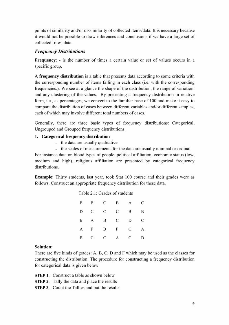
Table: Data given to present a Histogram

Class Boundaries

Class Mark

Frequency Cumulative Frequency (less than type)

Cumulative Frequency (more than type)

5.5 – 11.5 8.5 2 2 20 11.5 – 17.5 14.5 2 4 18 17.5 – 23.5 20.5 7 11 16 23.5 – 29.5 26.5 4 15 9 29.5 – 35.5 32.5 3 18 5 35.5 – 41.5 38.5 2 20 2

ii. Frequency Polygon A frequency polygon is a line graph drawn by taking the frequencies of the classes along the vertical axis and their respective class marks along the horizontal axis. Then join the cross points by a free hand curve.

Example: Construct a frequency polygon for the frequency distribution of the time spent by the automobile workers that we have seen in example 2.9.

Figure: Number of minutes spent by the automobile workers. iii. Cumulative Frequency Polygon (Ogive)

It is a graph obtained by plotting the cumulative frequencies of a distribution against the boundaries used to form the cumulative frequencies. Example: Construct an ogive for the time spent by the automobile workers.

17  

3. Measures of Central Tendency

Introduction Measures of Central Tendency give us information about the location of the center of the distribution of data values. A single value that describes the characteristics of the entire mass of data is called measures of central tendency. We will discuss briefly the three measures of central tendency: mean, median and mode in this unit.

Suppose we have a random sample of n values of some measurement X. The values are X1, X2, . . ,Xn. We want to summarize the information contained in this sample as regards an "average" level. An average is a numerical value that indicates the middle point or central region of the raw data. Mathematically summarize data in order to make appropriate comparisons.

Objectives of measures of central tendency Objectives of measuring central tendency are:

• To get a single value that represent(describe) characteristics of the entire data • To summarizing/reducing the volume of the data • To facilitating comparison within one group or between groups of data • To enable further statistical analysis

The Summation Notation (∑): Let a data set consists of a number of observations, represents by where n denotes the number of observations in the data and

is the ith observation. Then, is the sum of all the observation ∑=i

ix1

N

∑

xxx n.,..,, 21

ix

For instance a data set consisting of six measurements 21, 13, 54, 46, 32 and 37 is represented by and where = 21, = 13, = 54, = 46, = 32 and = 37.

54321 ,,,, xxxxx 6x 1x 2x 3x 4x 5x

6x

Their sum becomes 21+13+59+46+32+37=208. ∑=

=6

1iix

Similarly =

222

21 ... nxxx +++ ∑

=

n

iix

1

2

Some Properties of the Summation Notation

1. = where c is a constant number. ∑=

n

ic

1

cn.

2. where is a constant number ∑ ∑= =

=n

i

n

iii xbxb

1 1. b

3. where a and b are constant numbers ∑= =

+=+n

i

n

iii xbanbxa

1 1.)(

4. ∑∑∑===

±=±n

ii

n

ii

n

iii yxyx

111)(

5. ∑∑∑===

≠n

ii

n

ii

n

iii yxyx

111

18  

Important Characteristics of a Good Average: A typical average should posses the following:  • It should be rigidly defined. • It should be based on all observation under investigation. • It should be as little as affected by extreme observations. • It should be capable of further algebraic treatment. • It should be as little as affected by fluctuations of sampling. • It should be ease to calculate and simple to understand.

i. Mean The mean of a sample is determined by summing up all the data values of the sample and dividing this sum by the total number of data values.

There are four types of means which are suitable for a particular type of data. These are

1. Arithmetic Mean 2. Geometric Mean 3. Harmonic Mean

Arithmetic Mean Arithmetic mean is defined as the sum of the measurements of the items divided by the total number of items. It is usually denoted by x .

Suppose are n observed values in a sample of size n from a population

of size N, n<N then the arithmetic mean of the sample, denoted by xx n..,, 21x

x is given by

nx

nx....xx= in21 ∑=

+++X

If we take an entire population Mean is denoted by µ and is given by:

NN= N21 =μ

xx....xx i∑+++

Example: Consider the samples given for the two routes as follows:

For route A, the sample values are: 38 41 34 46 36 30 37 36 32 40 For route B the sample values are: 28 32 36 30 31 37 36 80 32 34 31 Find the arithmetic mean for the two routes. Solution: For route A, the sample values were: 38 41 34 46 36 30 37 36 32 40.

0.3710370

1040 + 32+ 36 + 37+ 30 + 36 + 46+ 34+ 1 4+ 38 = x == minutes

For route B the sample values were: 28 32 36 30 31 37 36 80 32 34 31.

0.3711407

1131 34+ 32+ 80 + 36+ 37 + 31 + 30+ 36+32+ 28 = x ==

+ minutes

19  

When the numbers occur with frequencies , respectively, then mean can be expressed in a more compact form as

, ,   , … ,   , ,   , … ,  

 ∑∑

Example Calculate the arithmetic mean of the sample of numbers of people living in twelve houses in a street: 3 2 4 4 3 1 2 5 3 3 8 1.

25.31239

121 8 3+ 3+ 5+ 2+ 1 + 3 + 4+ 4+2+ 3 = x ==

+ +

The information in the sentence above can be written in a table, as follows.

Value, x 1 2 3 4 5 8 Frequency, f 2 2 4 2 1 1

 

The formula for the arithmetic mean for data of this type is

∑∑

In this case we have:

.25.31239

128581242

11242281514241

==3222 +++++

=++++++×+

=x ×+×+× × + ×

The mean numbers of people living in twelve houses in a street is 3.25. Arithmetic Mean for Grouped Frequency Distribution

If data are given in the form of continuous frequency distribution, the sample mean is:

fff

mfmfmff

mf

k

kkk

ii

iii

x+++

+++==

∑

∑

=

=

...

...

21

2211

1

1

i

nfi

i =∑=1

thi

k

Where m is the class mark of the class; i = 1, 2, …, k; th fi is the frequency of the i class and k = the number of classes

k

Note that = the total number of observations.

Example: The following table gives the height (inches) of 100 students in a college. Class Interval (CI) Frequency (f)60 - 62 5 62 – 64 18 64 – 66 42 66 – 68 20 68 – 70 8 70 – 72 7 Total 100

Calculate the mean?

20  

Solution:

∑

∑

=

== k

ii

k

iii

f

mfx

1

1

1001

==∑=

nfk

ii ,

∑

∑

=

== k

ii

k

iii

f

mfx

1

1 =1006558 = 65.58

The mean height of students is 65.58

Properties of the Arithmetic Mean

The sum of the deviations of the items from their arithmetic mean is zero. This means, the algebraic sum of the deviations of a set of numbers from

their mean

nxxx .,..,, 21

x is zero. That is

The sum of the squares of the deviations of a set of observations from any number, say A, is minimum when A= . That is, ∑   ∑

0)(1

=−∑=

n

ii xx

When a set of observations is divided into k groups and 1x the mean of 1nservations of group 1,

isob 2x the mean of n bservations of group2, …, is 2 o kx is the mean of observations of group k , then the combined mean ,denoted by kn x , of all observations taken together is given by

If the mean of isnxxx .,..,, 21 x , then a) the mean of kxkxkx n ±±± .,..,, 21 will be kx ± b) The mean of will benkxkxkx .,..,, 21 xk .

Example

Last year there were three sections taking Stat 200 course. At the end of the semester, the three sections got average marks of 80, 83 and 76. There were 28, 32 and 35 students in each section respectively. Find the mean mark for the entire students.

Solution:

==++++

=++++

=95

7556353228

)76(35)83(32)80(28

321

332211

nnnxnxnxn

x 79.54

Weighted Arithmetic Mean In finding arithmetic mean, all items were assumed to be of equally importance (each value in the data set has equal weight). When the observations have different weight, we use weighted average. Weights are assigned to each item in proportion to its relative importance.

21  

If represent values of the items and are the corresponding weights, then the weighted mean,

kxxx .,..,, 21 kwww ,...,, 21

)( wx is given by

1 1 2 2 1

1 2

1

......

k

i ik k i

w kk

ii

w xw x w x w xX

w w w w

=

=

+ + += =

+ + +

∑

∑

Example: A student’s final mark in Mathematics, Physics, Chemistry and Biology are respectively 82, 80, 90 and 70.If the respective credits received for these courses are 3, 5, 3 and 1, determine the approximate average mark the student has got for one course. Solution

We use a weighted arithmetic mean, weight associated with each course being taken as the number of credits received for the corresponding course.

Therefore 17.821353

)701()903()805()823(=

+++×+×+×+×

==∑∑

i

iiw w

xwx

Average mark of the student for one course is approximately 82.

Geometric Mean The geometric mean like arithmetic mean is calculated average. It used when observed values are measured as ratios, percentages, proportions, indices or growth rates. The geometric mean, G.M. of a series of numbers is defined as xnxx .,..,, 21

nnxxxGM .....

21= ,

Properties of geometric mean a. Its calculations are not as such easy. b. It involves all observations during computation c. It may not be defined even it a single observation is negative. d. If the value of one observation is zero its values becomes zero.

Remark: 1) When the observed values have the corresponding frequencies xnxx .,..,, 21

f nff .,..,, 21 respectively, the geometric mean is obtained by

nkxxx fffGM k..... 21

21=

2) The above formula can also be used whenever the frequency distribution are grouped (continuous), class marks of the class intervals are considered as im

n

kmmm fffGM k..... 2121

= Where ∑=

=n

iifn

1

Example: Compute the geometric mean of the following values: 2, 8, 6, 4, 10, 6, 8, 4

Solution:

22  

nkxxx fffGM k..... 21

21= = 8 1221 108642 ...2.

8 106436162 xxxxGM = 8 737280= = 5.41

The geometric mean for the given data will be 5.41

Harmonic Mean It is a suitable measure of central tendency when the data pertains to speed, rate and time. The harmonic mean is defined as the reciprocal of the arithmetic mean of the reciprocal of the individual observations. If are n observations, then harmonic mean can be represented by the following formula:

xnxx .,..,, 21

xxx n

n

ii

nnHM1....11

11

++==

∑ =

If the data arranged in the form of frequency distribution

xfxf

ff

xf

f

kk

k

n

i

i

k

i i

i

HM

++

++==

∑∑

=

=

........1

.....1

11

1

1

1

Properties of harmonic mean i. It is based on all observation in a distribution.

ii. Used when a situations where small weight is give for larger observation and larger weight for smaller observation

iii. Difficult to calculate and understand iv. Appropriate measure of central tendency in situations where data is in

ratio, speed or rate Example: A motorist travels 480km in 3 days. She travels for 10 hours at rate of 48km/hr on 1st day, for 12 hours at rate of 40km/hr on the 2nd day and for 15 hours at rate of 32km/hr on the 3rd day. What is her average speed?

92.39

321

401

481

3=

++=HM

Note: Whenever the frequency distribution are grouped (continuous), class marks of the class intervals are considered as and the above formula can be used as im

∑ =

=n

ii

mf

nHM

1i

where mi is the class mark of ith class. ∑=

=n

iifn

1

Relations among different means

1. If all the observations are positive we have the relationship among the three means given as: HMGMx ≥≥

23  

2. For two observations GMHMx =* 3. HMGMx == if all observation are positive and have equal magnitude.

ii. Median The median of a set of items (numbers) arranged in order of magnitude (i.e. in an array form) is the middle value or the arithmetic mean of the two middle values. We shall denote the median of by x~ . nxxx .,..,, 21

Median for Ungrouped Frequency Distribution

We arrange the sample in ascending order of the variable of interest. Then the median is the middle value (if the sample size n is odd) or the average of the two middle values (if the sample size n is even).

For ungrouped data the median is obtained by

⎪⎪⎪⎪

⎩

⎪⎪⎪⎪

⎨

⎧

+

=

⎟⎠⎞

⎜⎝⎛ +⎟

⎠⎞

⎜⎝⎛

⎟⎠⎞

⎜⎝⎛ +

evenisnitemsofnumbertheif

itemitem

oddisnitemsofnumbertheifitem

x nn

n

thth

th

,,,2

,,,

~

122

21

Example: Compute the medians for the following two sets of data

A: 38 41 34 46 36 30 37 36 32 40.

B: 28 32 36 30 31 37 36 80 32 34 31

Solution

For A, the sample times in ascending order are: 30 32 34 36 36 37 38 40 41 46.

The two middle values have been underlined, So the median time ( x~ ) =

5.3623736

=+ minutes.

For B, the sample times in ascending order are: 28 30 31 31 32 32 34 36 36 37 80.

The middle value has been underlined. So the median time ( x~ ) = 32 minutes.

The median is easy to calculate for small samples and is not affected by an "outlier" - atypical value in the sample, e.g. the value 80 in the sample for route B. It is valid for ranked (ordinal) as well as interval/ratio (numeric) data.

Median for Grouped Frequency Distribution

For grouped data the median, obtained by interpolation method, is given by  

24  

Where lower class boundary of the median class =medL=F Sum of frequencies of all class lower than the median class (in other words it

is the cumulative frequency immediately preceding the median class) Frequency of the median class and =medf Class width =WThe median class is the class with the smallest cumulative frequency greater than or equal to 2

n .

Example: Calculate the median for the following frequency distribution.

Class Class Boundary

Frequency Less than Cum. Freq (CF)

0 – 5 5 5 5 – 10 8 13 10 – 15 10 23 15 – 20 8 31 20 – 25 5 36

Solution: To obtain the median class we divide 36 by 2. That is, 182

362 ==n

Thus the smallest cumulative frequency that contains 18 is 23. Hence the median class is the 3rd class which is 10 – 15.

Therefore median is  

Where 9.5, 13 sum of frequencies of all class lower than the 3rd class =medL =F 10, frequency of the 3rd class and, =medf =W 6, class width

5.12

35.910

131865.9~

=+=

⎟⎠⎞

⎜⎝⎛ −

+=x

iii. Mode The mode or the modal value is the most frequently occurring score/observation in a series and denoted by . A data set may not have a mode or may have more than one mode. A distribution is called a bimodal distribution if it has two data values that appear with the greatest frequency. If a distribution has more than two modes, then the distribution is multimodal. If a distribution has no modes, then the distribution is non-modal.

x̂

Example: Consider the following data:

Data X: 3, 4, 6, 12, 31, 8, 9, 8 the Mode ( ) = 8 x̂Data Y: 6, 8, 12, 13, 11, 12, 6 the Mode ( ) = 6 and 12 x̂Data Z: 2, 6, 3, 5, 7, 8, 12, 11 No Mode Note that in some samples there may be more than one mode or there may not be a mode. The mode is not a suitable measure of central tendency in these cases.

25  

Mode for Grouped Frequency Distribution For grouped data, the mode is found by the following formula:

WLx ⎟⎟⎠

⎜⎜⎝ Δ+Δ

+=21

1modˆ ⎞⎛ Δ

Where lower class boundary of the modal class =modL

11 ff −=Δ , 22 ff −=Δ =1f Frequency of the modal class =1f Frequency of the class immediately preceding the modal class =2f Frequency of the class immediately follows the modal class =W the class width

The modal class is the class with the highest frequency in the distribution.

Example: Find the mode for the frequency distribution of the birth weight (in kilogram) of 30 children given below.

Weight 1.9-2.3 2.3-2.7 2.7-3.1 3.1-3.5 3.5-3.9 3.9-4.3

No. of children 5 5 9 4 4 3

Solution:

2.7- 3.1 is the modal class since it has the highest frequency and4591 =−=Δ 5492 =−=Δ 7.2mod =L

878.24.0*54

47.2ˆ =⎟⎠⎞

⎜⎝⎛

++=x  

The Relationship of the Mean, Median and Mode • In the case of symmetrical distribution; mean, median and mode coincide.

That is mean=median = mode. However, for a moderately asymmetrical (non symmetrical) distribution, mean and mode lie on the two ends and median lies between them and they have the following important empirical relationship: Mean – Mode = 3(Mean - Median) ⇒ ( )xxxx ~3ˆ −=−

Example In a moderately asymmetrical distribution, the mean and the median are 20 and 25 respectively. What is the mode of the distribution?

Solution: Mode = 3median – 2mean = 3(25) – 2(20) = 75 – 40

= 35, hence the mode of the distribution will be 35.

4. MEASURES OF VARIATION (DISPERSION)

Introduction and objectives of measuring variation

We have seen that averages are representatives of a frequency distribution. But they fail to give a complete picture of the distribution. They do not tell anything about the spread or dispersion of observations within the distribution. Suppose that we have the distribution of yield (kg per plot) of two rice varieties from 5 plots each.

26  

Variety 1: 45 42 42 41 40 Variety 2: 54 48 42 33 30

The mean yield of both varieties is 42 kg. The mean yield of variety 1 is close to the values in this variety. On the other hand, the mean yield of variety 2 is not close to the values in variety 2. The mean doesn’t tell us how the observations are close to each other. This example suggests that a measure of central tendency alone is not sufficient to describe a frequency distribution. Therefore, we should have a measure of spreads of observations. There are different measures of dispersion.

Objectives of measuring variation

• To describe dispersion (variability) in a data. • To compare the spread in two or more distributions. • To determine the reliability of an average.

Note: The desirable properties of good measures of variation are almost identical with that of a good measure of central tendency.

Absolute and relative measures Absolute measures of dispersion are expressed in the same unit of measurement in which the original data are given. These values may be used to compare the variation in two distributions provided that the variables are in the same units and of the same average size. In case the two sets of data are expressed in different units, however, such as quintals of sugar versus tones of sugarcane or if the average sizes are very different such as manager’s salary versus worker’s salary, the absolute measures of dispersion are not comparable. In such cases measures of relative dispersion should be used. A measure of relative dispersion is the ratio of a measure of absolute dispersion to an appropriate measure of central tendency. It is a unitless measure.

Types of Measures of Variation

i. The range and relative range Range(R) is defined as the difference between the maximum and minimum observations in a set of data.

Range Maximum value Minimum value= − It is the crudest absolute measures of variation. It is widely used in the construction of quality control charts and description of daily temperature. Properties of range

It is affected by extreme values. It does not take into account all observations. It is easy to calculate and simple to understand. It does not tell anything about the distribution of values in the set of data

relative to some measures of central tendency.

Relative range (RR) is defined as. .

RangeRRMax value Min value

=+

ii. The mean deviation and coefficient of mean deviation

Mean deviation (MD) is the average of the absolute deviations taken from a central value, generally the mean or median.

1 1| | | |

n k

i i ii i

X

X X X X fMD

n n= =

− −= =∑ ∑

, 1 1| | | |

n k

i ii i

X

iX X X XMD

n n= =

− −= =∑ ∑

%

% % f

27  

Example: Calculate the mean deviation about the median and about the mean of the following scores of students in a certain test. 6,7,7,10,10

1 1.65 5

iXMD

n== = = =

| || 6 8 | | 7 8 | *2 |10 8 | *2 8

k

i iX X f−− + − + −∑

1| |

| 6 7 | | 7 7 | *2 |10 7 | *2 7 1.45 5

k

i ii

X

X X fMD

n=

−− + − + −

= = =∑

%

%

=

Note: In case of grouped data, the mid-point of each class interval is treated as and we can use the above formula. Besides, X XMD MD≥ % Properties of mean deviation

It is relatively simple to understand as compared to standard deviation. Its computation is simple. It is less affected by extreme values than standard deviation. It is better than the range and QD since it is based on all observations. It is not suitable for further statistical treatment.

iii. Variance, standard deviation and coefficient of variation The variance is the average of the squares of the distance each value is from the mean. The symbol for the population variance is σ2. Let 1 2, ,..., Nx x x be the measurements on N population units then, the population variance is given by the formula:

2

12 2

2 1 1( )

N

iN Ni

i ii i

xx x

NN N

μσ

=

= =

⎛ ⎞⎜ ⎟⎝ ⎠− −

= =

∑∑ ∑

,

Where µ is population mean and N is population size

Let 1 2, ,..., nx x x be the measurements on n sample units then, the sample variance is denoted by S2, and its formula is

2

12 2

2 1 1

( )

1 1

n

in ni

i ii i

xx x x

nSn n

=

= =

⎛ ⎞⎜ ⎟⎝ ⎠− −

= =− −

∑∑ ∑

Where x is the sample mean and n is the sample size.

Standard deviation, denoted by σ or S, is the square root of the variance. That is, Population standard deviation 2σ σ= and sample standard deviation 2S S= . Example: For a newly created position, a manager interviewed the following numbers of applicants each day over a five-day period: 16, 19, 15, 15, and 14. Find the variance and standard deviation.

Solution:

5

1 16 19 15 15 14 79 15.85 5 5

ii

xx = + + + += = = =∑

28  

52

2 22 1

( )(16 15.8) ... (14 15.8) 14.8 3.7

5 1 4 4

ii

x xS =

−− + + −

⇒ = = = =−

∑

Or

( )

2

2512 2 2

2 1

16 ... 14 624116 ... 14 1263 14.85 5 5 3.75 1 4 4 4

n

ii

ii

xx

S

=

=

⎛ ⎞⎜ ⎟ + +⎝ ⎠− + + − −

= = = =−

∑∑

=

For grouped frequency distribution, the formula for variance is

2

12 2

2 1 1( )

1 1

k

i ik ki

i i i ii i

f xf x x f x

nSn n

=

= =

⎛ ⎞⎜ ⎟⎝ ⎠− −

= =− −

∑∑ ∑

Where is the number of classes, k ix is the class mark of class i and 1

k

ii

n f=

= ∑Properties of variance

The unit of measurement of the variance is the square of the unit of measurement of the observed values. It is one of its limitations.

The variance gives more weight to extreme values as compared to those which are near to the mean value, because the difference is squared in variance.

It is based on all observations in the data set. Properties of standard deviation

Standard deviation is considered to be the best measure of dispersion and is used widely.

There is, however, one difficulty with it. If the unit of measurement of variables of two series is not the same, then their variability cannot be compared by comparing the values of standard deviation.

Uses of the variance and standard deviation The variance and standard deviations can be used to determine the spread of

data, consistency of a variable and the proportion of data values that fall within a specified interval in a distribution.

If the variance or standard deviation is large, the data is more dispersed. This information is useful in comparing two or more data sets to determine which is more (most) variable.

Finally, the variance and standard deviation are used quite often in inferential statistics.

Coefficient of variation (CV)

The standard deviation is an absolute measure of dispersion. The corresponding relative measure is known as the coefficient of variation (CV). Coefficient of variation is used in such problems where we want to compare the variability of two or more different series. Coefficient of variation is the ratio of the standard deviation to the arithmetic mean, usually expressed in percent:

*100%sCVx

=

A distribution having less coefficient of variation is said to be less variable or more consistent or more uniform or more homogeneous.

29  

Example: Last semester, the students of two departments, A and B took Stat 276 course. At the end of the semester, the following information was recorded. Dept A Dept B

Mean score 79 64 SD 23 11

Compare the relative dispersion of the two departments. 23*100% *100 29.11%79

AA

A

sCVx

= = = , 11*100% *100 17.19%64

BB

B

sCVx

= = =

Since ACV > , the variation is department A is greater. Or, in department B the distribution of the marks is more uniform (consistent).

BCV

Exercise: The mean weight of 20 children was found to be 30 kg with variance of 16kg2 and their mean height was 150 cm with variance of 25cm2. Compare the variability of weight and height of these children.

iv. The standard scores A standard score is a measure that describes the relative position of a single score in the entire distribution of scores in terms of the mean and standard deviation. It also gives us the number of standard deviations a particular observation lie above or below the mean.

Standard score, ,x x XZ or ZS

μσ− −

= =

Where x is the value of the observation, / Xμ and / Sσ are the mean and standard deviation of the respectively.

Interpretation:

,

,,

Negative the observation lies below the meanIf Z is Positive theobservation lies above the mean

Zero the observationequals to the mean

⎧⎪⎨⎪⎩

Example: Two sections were given an exam in a course. The average score was 72 with standard deviation of 6 for section 1 and 85 with standard deviation of 5 for section 2. Student A from section 1 scored 84 and student B from section 2 scored 90. Who performed better relative to his/her group? Solution: Section 1: x = 72, S = 6 and score of student A from Section 1; A x = 84

Section 2: x = 85, S = 5 and score of student B from Section 2; B x = 90

Z-score of student A: 84 72 26

A AA

A

x XZS− −

= = =

Z-score of student B: 90 85 15

B BB

B

x XZS− −

= = =

From these two standard scores, we can conclude that student A has performed better relative to his/her section students because his/her score is two standard deviations above the mean score of selection 1 while the score of student B is only one standard deviation above the mean score of section 2 students.

Exercise: A student scored 65 on a calculus test that had a mean of 50 and a standard deviation of 10; she scored 30 on a algebra test with a mean of 25 and a standard deviation of 5. Compare her relative positions on each test.

30  

v. Skewness and kurtosis Skweness refers to lack of symmetry in a distribution. If a distribution is not

symmetrical we call it skewed distribution. Note that for a symmetrical and unimodal distribution: Mean = median = mode

Measure of skewness:

3ˆx x

sα − Pearsonian coefficient of skewness (Pcsk) defined as: =

Interpretation: 3

0,0,0,

the distribution isnegatively skewedIf the distribution is positively skewed

the distribution is symetricalα

<⎧⎪>⎨⎪=⎩

In moderately skewed distributions: Mode = mean- 3(mean-median) 33( )x x

sα −

⇒ =%

Note: in a negatively skewed distribution larger values are more frequent than smaller values. In a positively skewed distribution smaller values are more frequent than larger values. Exercise: If the mean, mode and s.d of a frequency distribution are 70.2, 73.6, and 6.4, respectively. What can one state about its skeweness?

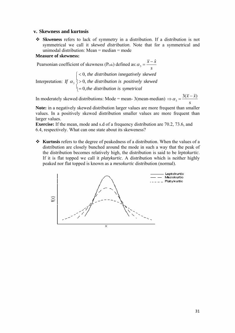
Kurtosis refers to the degree of peakedness of a distribution. When the values of a distribution are closely bunched around the mode in such a way that the peak of the distribution becomes relatively high, the distribution is said to be leptokurtic. If it is flat topped we call it platykurtic. A distribution which is neither highly peaked nor flat topped is known as a mesokurtic distribution (normal).

31